1 Introduction

In October 2018, a portrait titled Edmond de Belamy sold at Christie's auction house for $432,500, roughly 45 times its estimate. The portrait was not the work of a human artist; it was produced by a generative adversarial network trained on thousands of historical portraits. The buyer received a canvas printed with pixels dreamt up by a neural network that had never held a brush, never visited a museum, and never experienced the emotion a portrait tries to capture. Yet the result was compelling enough that seasoned art collectors opened their wallets.

This was just the opening act. By 2024, generative models could produce photorealistic images of people who have never existed (StyleGAN), compose four-minute songs complete with vocals and instrumentation from a one-sentence text prompt (Suno), generate sixty-second cinematic video clips from a paragraph of text (Sora), design novel proteins that fold into shapes never seen in nature (RFdiffusion), and forecast global weather fifteen days ahead more accurately than the world's best supercomputer-driven physics simulations (GenCast).

Behind each of these feats lies a common mathematical question:

This question may sound abstract, but its answer has reshaped entire industries and raised urgent societal questions about truth, creativity, and privacy. This book develops the mathematical machinery needed to answer it rigorously. We begin in this chapter with an informal, panoramic tour of the landscape: what generative models are, how they are classified, where they have been applied to stunning effect, what dangers they pose, and how we evaluate whether they are any good. Along the way, we preview the key mathematical ideas (probability distributions, divergence measures, variational inference, and stochastic processes) that will be developed in full detail in subsequent chapters.

What Is Generative Modelling?

Imagine you are shown a thousand photographs of cats. After studying them, you develop an intuitive sense of what a “typical” cat photograph looks like: the shapes, colours, textures, and poses that tend to appear. Now imagine being asked to draw a new cat photograph from memory, one that looks realistic but is not a copy of any photo you have seen. This is, in essence, what a generative model does: it studies a collection of examples, extracts their statistical regularities, and uses those regularities to produce new examples.

More formally:

Generative vs. Discriminative Models

If you have taken a course in machine learning, you have likely encountered discriminative models, classifiers and regressors that predict a label $y$ from input features $𝐱$. It is instructive to contrast these with generative models:

• A discriminative model learns the conditional distribution $p(y|𝐱)$. It answers: “given this input, what is the label?”

• A generative model learns the joint distribution $p(𝐱,y)$, or in the unsupervised setting simply $p(𝐱)$. It answers: “what does the data look like?”

By learning $p(𝐱,y)$, a generative model can in principle also perform classification via Bayes' rule: $$p(y|𝐱)=\frac{p(𝐱|y)p(y)}{p(𝐱)}.$$ However, in practice, discriminative models typically achieve higher classification accuracy because they focus all modelling capacity on the decision boundary rather than on modelling the full data distribution. The power of generative models lies elsewhere: they can synthesise new examples, detect anomalies, impute missing data, learn meaningful latent representations, and, as we will see in this chapter, enable applications that discriminative models simply cannot.

Why Is Generative Modelling Hard?

To appreciate why generative modelling is challenging, consider a seemingly simple task: modelling $28\times 28$ grayscale images of handwritten digits (the MNIST dataset). Each image is a vector $𝐱\in {\{0,1,\dots ,255\}}^{784}$.

This challenge, a manifestation of the curse of dimensionality, motivates the central strategies of modern generative modelling:

1. Latent variables: assume the high-dimensional data $𝐱$ is generated from a low-dimensional latent code $𝐳$ via a stochastic process $𝐱\sim p_{\theta }(𝐱|𝐳)$. The intuition is that a handwritten “7” can be described by a handful of factors (stroke angle, thickness, whether it has a crossbar) rather than by 784 independent pixel values.

2. Neural parameterisation: use deep neural networks to represent complex, nonlinear mappings between the latent space and the data space.

3. Clever training objectives: design loss functions that avoid the intractable computation of normalising constants or partition functions.

Each family of generative models makes different choices along these axes, leading to the taxonomy we describe next.

A Taxonomy of Generative Models

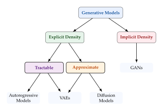
Generative models can be organised along several axes, but the most fundamental distinction concerns how the model represents the data distribution $p_{\theta }(𝐱)$. fig:taxonomy presents an overview.

Explicit Density Models

Explicit density models define the probability density $p_{\theta }(𝐱)$ in a form that can be written down and (at least in principle) evaluated. They are further divided by whether the likelihood computation is tractable or only approximate.

Tractable density models.

• Autoregressive models decompose the joint distribution using the chain rule of probability: $$p_{\theta }(𝐱)=\prod _{i=1}^d{p}_{\theta }(x_i|x_1,\dots ,x_{i-1}).$$ Each conditional is parameterised by a neural network. For images, PixelCNN generates one pixel at a time, scanning left-to-right and top-to-bottom. For audio, WaveNet generates one audio sample at a time (typically 16,000 per second of speech). For text, GPT-style transformers generate one token at a time; this is the architecture behind ChatGPT and similar large language models. Exact likelihood computation is straightforward, but sampling is inherently sequential.

• Normalizing flows learn an invertible transformation $f_{\theta }:{\mathrm{ℝ}}^d\to {\mathrm{ℝ}}^d$ that maps a simple base distribution $p_{𝐳}(𝐳)$ (typically a standard Gaussian) to the data distribution. The change-of-variables formula gives the exact density: (Change OF Variables)$$\begin{array}{ccc}& p_{\theta }(𝐱)=p_{𝐳}(f_{\theta }^{-1}(𝐱))\cdot \left|\det \frac{\partial f_{\theta }^{-1}}{\partial 𝐱}\right|.& \text{<span class="tml-eqn"></span>}\end{array}$$ Think of it as learning a smooth, reversible “warping” of a simple bell curve into a complex data distribution. Both sampling ($𝐱=f_{\theta }(𝐳)$, $𝐳\sim p_{𝐳}$) and likelihood evaluation are efficient, but the requirement that $f_{\theta }$ be invertible with a tractable Jacobian determinant constrains the network architecture.

Approximate density models.

• Variational autoencoders (VAEs) introduce latent variables $𝐳$ and define $p_{\theta }(𝐱)=\int p_{\theta }(𝐱|𝐳)p(𝐳)\mathrm{d}𝐳$. This integral is typically intractable, so VAEs optimise a tractable lower bound, the evidence lower bound (ELBO): $$\log p_{\theta }(𝐱)\ge {𝔼}_{q_{\varphi }(𝐳|𝐱)}[\log p_{\theta }(𝐱|𝐳)]-D_{\mathrm{KL}}(q_{\varphi }(𝐳|𝐱)\Vert p(𝐳)).$$ Intuitively, a VAE learns two networks: an encoder that compresses data into a compact code, and a decoder that reconstructs data from the code. The magic is that the code space is structured smoothly enough that you can sample new codes and decode them into novel, realistic data.

• Diffusion models define a forward noising process that gradually corrupts data into pure noise. Imagine slowly adding static to a photograph until it becomes indistinguishable from random TV snow. The model then learns to reverse this process step by step, starting from pure noise and progressively “denoising” until a clean image emerges. Diffusion models currently produce the highest-quality image and video samples among all generative model families and are the engine behind DALL$\cdot$E, Stable Diffusion, and Sora.

Implicit Density Models

Implicit density models do not define $p_{\theta }(𝐱)$ at all. Instead, they learn a deterministic mapping $G_{\theta }:𝐳\mapsto 𝐱$ from a noise vector $𝐳\sim p_{𝐳}$ to the data space, such that the distribution of $G_{\theta }(𝐳)$ approximates $p_{\mathrm{data}}(𝐱)$.

• Generative adversarial networks (GANs) train two networks simultaneously in a game-theoretic framework. A generator $G_{\theta }$ produces fake samples and tries to fool a discriminator $D_{\varphi }$, which tries to tell real samples from fakes. The training is formulated as a minimax game: $$\underset{\theta }{\min }\underset{\varphi }{\max }{𝔼}_{𝐱\sim p_{\mathrm{data}}}[\log D_{\varphi }(𝐱)]+{𝔼}_{𝐳\sim p_{𝐳}}\left[\log \right(1-D_{\varphi }(G_{\theta }(𝐳))\left)\right].$$ Think of it as a counterfeiter (generator) and a detective (discriminator) locked in an escalating arms race. The counterfeiter keeps improving until the detective can no longer tell real from fake, at which point the counterfeiter has learned to produce perfect imitations. GANs produce remarkably sharp and realistic samples, but training can be unstable and they provide no mechanism for likelihood evaluation.

Comparison of Model Families

Table 1 summarises the key trade-offs between the main families of generative models.

Property	Autoregressive	Flows	VAEs	GANs	Diffusion
Exact likelihood	✓	✓	$\times$	$\times$	$\times$
Fast sampling	$\times$	✓	✓	✓	$\times$
Sample quality	High	Medium	Medium	High	Very High
Training stability	High	High	High	Low	High
Latent representation	$\times$	✓	✓	$\times$	$\times$
Mode coverage	High	High	High	Low	High

The Generative Pipeline

Regardless of the specific model family, every generative modelling workflow follows a common pipeline, illustrated in fig:gen-pipeline.

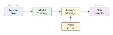
The pipeline consists of three stages:

1. Data collection and preprocessing. Assemble a representative dataset $\{{𝐱}_1,\dots ,{𝐱}_n\}$ from the domain of interest. For images, this typically involves resizing, normalising pixel values to $[\mathrm{0,1}]$ or $[-\mathrm{1,1}]$, and possibly applying data augmentation. The quality and diversity of the training data fundamentally limits what the model can learn.

2. Model training. Choose a model family and optimise its parameters $\theta$ by minimising a loss function that measures the discrepancy between $p_{\theta }$ and $p_{\mathrm{data}}$. The choice of loss function is what fundamentally distinguishes different model families: maximum likelihood for autoregressive models and flows, the ELBO for VAEs, adversarial loss for GANs, and score matching for diffusion models.

3. Sampling and evaluation. Draw noise $𝐳$ from a simple prior distribution and pass it through the learned model to obtain a new sample ${𝐱}_{\mathrm{new}}$. Evaluate the quality of the generated samples using quantitative metrics and qualitative inspection.

Applications in Vision and Graphics

Perhaps the most visible applications of generative models are in computer vision and graphics. We describe several key tasks below, explaining what each one means and why it matters.

Image Synthesis

Image synthesis refers to generating entirely new images from scratch: images of objects, scenes, or people that have never existed. The progress in this area has been breathtaking:

• In 2014, the first GAN could generate blurry, $64\times 64$ images of faces and bedrooms.

• By 2019, StyleGAN2 produced $1024\times 1024$ photorealistic faces that most humans could not distinguish from real photographs.

• In 2022, text-to-image models like DALL$\cdot$E 2, Midjourney, and Stable Diffusion enabled anyone to generate detailed images from natural language descriptions such as “an astronaut riding a horse on Mars, oil painting style.”

• In March 2025, OpenAI's GPT-4o integrated image generation directly into a chatbot, and millions of users converted their personal photographs into Studio Ghibli-style artwork within days. The demand was so intense that OpenAI's CEO reported it was “melting their GPUs.”

Style Transfer

The key insight behind neural style transfer [10] is that a pretrained convolutional neural network (such as VGG) separates content (captured by high-level feature activations) from style (captured by correlations between feature maps, measured via Gram matrices). By optimising an image to match the content features of one image and the style features of another, we can blend the two.

Style transfer has moved from a research curiosity to a widely used consumer feature. Apps like Prisma brought it to smartphones; Adobe Firefly integrated it into professional creative workflows; and in 2023, Coca-Cola released a commercial (“Masterpiece”) in which paintings in a museum passed a bottle between artworks rendered in different artistic styles, all generated by AI.

Inpainting

Imagine you have a holiday photograph ruined by a passing stranger walking through the frame. With inpainting, you select the stranger, and the model fills in the region behind them, reconstructing the beach, the waves, the sand, as if the stranger had never been there. This requires the model to understand not just local texture (“the neighbouring pixels are sandy-coloured”) but also global semantics (“this region should contain a continuation of the shoreline”).

Modern inpainting is powered by diffusion models that condition on the known (unmasked) pixels and generate the masked region. Adobe Photoshop's “Generative Fill” (powered by the Firefly model), released in 2023, brought this capability to millions of creative professionals. Users can select any region and type a text prompt (e.g., “a red bicycle”), and the model generates content that blends seamlessly with the existing image. Canva similarly offers “Magic Eraser” and “Magic Edit” for consumer use.

Super-Resolution

This is an inherently ill-posed problem: many high-resolution images could have produced the same low-resolution version. Generative models handle this by learning the distribution of natural high-resolution images and sampling from it conditioned on the low-resolution input.

Super-resolution has found commercial applications in:

• Gaming: NVIDIA's DLSS (Deep Learning Super Sampling) renders games internally at lower resolution and uses a trained neural network to upscale frames in real time, delivering higher visual quality with less computational cost. DLSS has been integrated into hundreds of PC games.

• Television: Samsung's 2024 and 2025 Neo QLED 8K televisions use AI-powered upscaling to produce an 8K picture from 4K or 1080p sources in real time.

• Photography: Adobe Lightroom's “Super Resolution” doubles the linear resolution of RAW photographs using machine learning, and Topaz Gigapixel AI can enlarge images up to 600% before visible degradation.

• Satellite imagery: Enhancing the resolution of satellite photographs for environmental monitoring and urban planning.

Image-to-Image Translation

More broadly, many vision tasks can be framed as image-to-image translation: converting an image from one domain to another while preserving its structure. Examples include:

• Sketch-to-photo: turning a rough sketch into a photorealistic rendering.

• Day-to-night: transforming a daytime photograph into a nighttime scene.

• Satellite-to-map: converting aerial photographs into labelled maps.

• Cross-modality medical imaging: synthesising a CT scan from an MRI scan (or vice versa), eliminating the need for an additional radiation-exposing scan.

The Pix2Pix framework (paired image-to-image translation using conditional GANs) and CycleGAN (unpaired translation using cycle-consistency losses) are foundational architectures in this area.

Video Generation

The frontier of generative modelling has moved from still images to video. In February 2024, OpenAI previewed Sora, a text-to-video diffusion model capable of generating photorealistic sixty-second video clips from text prompts. Google followed with Veo, whose third version (Veo 3, released May 2025) became the first major model to generate synchronised audio (dialogue, sound effects, and ambient noise) alongside the visuals. Runway's Gen-3 was named one of TIME's “200 Best Inventions” of 2024 for its ability to create cinematic clips from text.

Applications in Science and Engineering

While image and video generation capture public attention, some of the most consequential applications of generative models are in scientific research and engineering. Here, the ability to model complex distributions translates directly into the ability to accelerate discovery.

Weather Prediction

For decades, weather forecasting has relied on numerical weather prediction (NWP): discretising the atmosphere into a three-dimensional grid and solving the Navier–Stokes equations forward in time using massive supercomputers. The European Centre for Medium-Range Weather Forecasts (ECMWF) runs the world's most accurate such system, using a 35-kilometre global grid updated every 12 hours.

In a remarkable series of results between 2023 and 2025, AI-based models surpassed this gold standard:

• GraphCast (Google DeepMind, 2023): a graph neural network trained on 39 years of reanalysis data that predicts hundreds of weather variables over 10 days at 0.25 resolution in under one minute on a single TPU. It outperformed the ECMWF's deterministic forecast on 90% of 1,380 verification targets.

• GenCast (Google DeepMind, 2024): a diffusion-based probabilistic weather model that generates ensembles of stochastic 15-day global forecasts. It outperformed the ECMWF's ensemble forecast on 97.2% of 1,320 evaluation targets, with superior performance on tropical cyclone tracks, extreme weather events, and wind-power forecasting. A single 15-day forecast takes 8 minutes on one TPU, compared to hours on a supercomputer.

Protein Design and Drug Discovery

Proteins are the molecular machines of life. Their function is determined by their three-dimensional shape, which in turn is determined by their amino acid sequence, a string of characters from a 20-letter alphabet. Predicting the shape from the sequence (the “protein folding problem”) has been one of biology's grand challenges for fifty years.

• AlphaFold 2 (Google DeepMind, 2020) solved the structure prediction problem with atomic-level accuracy, earning its creators Demis Hassabis and John Jumper the 2024 Nobel Prize in Chemistry.

• AlphaFold 3 (2024) went further: it uses a diffusion-based generative module that starts from a cloud of atoms and iteratively converges on the final structure. Unlike its predecessor, it can predict joint structures of complexes involving proteins, DNA, RNA, small-molecule drugs, and ions.

• RFdiffusion (Baker Lab, University of Washington, 2023) turns the problem around: instead of predicting a structure from a sequence, it generates entirely new proteins with desired shapes and functions. Built on the same diffusion framework, it designs novel protein binders, symmetric assemblies, and enzyme scaffolds. Hundreds of AI-generated designs have been experimentally validated in the laboratory, and they actually fold and function as predicted. David Baker, the lab's director, shared the 2024 Nobel Prize in Chemistry for computational protein design.

In drug discovery, generative models navigate vast chemical spaces to propose novel molecules. Insilico Medicine's AI-designed drug ISM001-055 (rentosertib), targeting idiopathic pulmonary fibrosis, showed positive results in a Phase IIa clinical trial in 2024: patients' lung function improved rather than merely declining more slowly. By the end of 2024, over 75 AI-derived molecules had reached clinical trials across the pharmaceutical industry.

Numerical Simulation and Fluid Dynamics

Traditional numerical methods for solving partial differential equations (PDEs), such as finite element methods for structural mechanics or computational fluid dynamics (CFD) for aerodynamics, are powerful but computationally expensive. A single CFD simulation of airflow around an aircraft can take days on a supercomputer cluster.

Generative models offer a radical alternative: learn the solution operator from data and produce solutions thousands of times faster:

• Fourier Neural Operators (FNO; Caltech/NVIDIA) parameterise integral kernels in Fourier space, learning entire families of PDE solutions rather than solving individual instances. The Geo-FNO variant achieves speedups of up to ${10}^5\times$ over traditional solvers.

• Diffusion models have been applied to generate turbulent flow fields directly, bypassing time-stepping simulations entirely. A 2024 study published in Nature Machine Intelligence showed that a diffusion model could generate three-dimensional turbulent particle trajectories at high Reynolds numbers, reproducing the heavy-tailed velocity distributions and anomalous scaling laws that characterise real turbulence.

• NVIDIA's CorrDiff model uses diffusion for climate downscaling, converting coarse-resolution global climate projections into high-resolution regional forecasts, achieving a $\mathrm{1,300}\times$ improvement in energy efficiency over the numerical model it replaces.

Mathematics and Automated Reasoning

In a development that would have seemed like science fiction a decade ago, generative models have begun making novel mathematical discoveries:

• FunSearch (Google DeepMind, 2023): an LLM paired with an automated evaluator discovered new constructions of large cap sets, a central problem in extremal combinatorics, that improved on bounds that had stood for 20 years. This was the first published instance of an LLM making a verifiable, novel mathematical discovery.

• AlphaProof (Google DeepMind, 2024): a reinforcement-learning agent that learns to find formal proofs. At the 2024 International Mathematical Olympiad, AlphaProof solved 4 out of 6 problems (including the hardest problem), achieving the equivalent of a silver medal, the first time any AI achieved medal-level performance at the IMO.

Materials Science

In November 2023, Google DeepMind's GNoME (Graph Networks for Materials Exploration) discovered 2.2 million new crystal structures, of which 380,000 are predicted to be thermodynamically stable, an order-of-magnitude expansion of all known stable materials. Among the discoveries: 52,000 new layered materials and 528 potential lithium-ion conductors relevant to next-generation batteries. Crucially, independent laboratories subsequently synthesised 736 of these predicted structures, confirming that the AI's predictions were physically valid.

Medicine

In medicine, generative models address a critical bottleneck: the scarcity of labelled data. Medical datasets are small (patient privacy limits sharing), expensive to annotate (requiring specialist physicians), and imbalanced (rare diseases have few examples). Generative models help by:

• Synthetic data augmentation: GANs and diffusion models generate realistic synthetic medical images (X-rays, MRIs, CT scans) that augment training sets for diagnostic classifiers without compromising patient privacy [2][3].

• Cross-modality synthesis: generating synthetic CT scans from MRI data for radiation therapy planning, eliminating the need for an additional scan that exposes the patient to ionising radiation.

• Foundation models: vision-language models for 3D medical imaging are beginning to enable automated report generation and interactive visual question-answering about scans.

Applications Beyond Vision

Music and Audio Generation

Generative models for audio have progressed from generating short clips of individual instruments to producing full, multi-instrument songs with vocals:

• Google's WaveNet (2016) was the first autoregressive model to generate raw audio waveforms with near-human speech quality.

• Suno (launched 2023) generates four-minute songs from text prompts, complete with vocals, instrumentation, and song structure. By 2025, its latest version could generate eight-minute tracks. In July 2025, a Suno user reportedly became the first AI-based music creator to sign a traditional record deal.

• Google's MusicFX enabled users to create over 10 million tracks within months of its 2024 release.

These developments have triggered significant legal battles. In 2024, the three major record labels filed $500 million lawsuits against Suno and Udio for training on copyrighted music. Both services subsequently reached settlement agreements, with Suno obtaining a licence to train on Warner Music Group's catalogue.

Natural Language Processing

Autoregressive language models represent one of the most commercially impactful applications of generative modelling. OpenAI's ChatGPT, launched in November 2022, reached 100 million monthly active users within two months, the fastest-growing consumer application in history. For comparison, TikTok took 9 months and Instagram about 2.5 years to reach the same milestone.

The underlying model, GPT-4 (released March 2023), is a multimodal autoregressive transformer that generates text one token at a time by sampling from $p_{\theta }(x_{t+1}|x_1,\dots ,x_t)$. It achieved human-level performance on numerous professional exams, including passing the bar exam in the 90th percentile. At its core, it is doing exactly what the chain rule decomposition in Explicit Density Models describes, modelling $p(𝐱)={\prod }_{i}p(x_i|x_{<i})$, but at an enormous scale (hundreds of billions of parameters trained on trillions of tokens).

The Dark Side: Deepfakes, Fraud, and Misinformation

The same technology that enables life-saving drug design and weather forecasting also enables deception at industrial scale. The dangers are not hypothetical; they are documented, ongoing, and escalating. Between 2023 and 2025, the number of reported deepfakes globally rose from approximately 500,000 to nearly 8 million, a 1,500% increase. Deepfake-related scam losses reached an estimated $1.1 billion worldwide in 2025.

Financial Fraud

In January 2024, a finance employee at Arup, the London-based multinational engineering firm, received a video call that appeared to include several senior colleagues, including the company's Chief Financial Officer. Every person on the call was a deepfake, an AI-generated recreation built from publicly available corporate videos. Convinced by what he saw, the employee authorised 15 wire transfers totalling HK$200 million (approximately US$25.6 million). The fraud was only discovered when the employee later checked with Arup's UK head office. This remains one of the largest single-incident deepfake financial frauds on record.

Election Interference

Deepfakes have targeted elections in at least 38 countries:

• Slovakia (September 2023): Two days before the parliamentary election, a fabricated audio recording surfaced that purported to capture the liberal party leader discussing plans to rig the vote. It went viral during the legally mandated pre-election media silence period, when news outlets were prohibited from discussing election-related content, meaning the deepfake could not be effectively debunked through mainstream channels. The pro-Russia candidate won. This is widely considered the first documented case of deepfake audio plausibly influencing a national election.

• United States (January 2024): Two days before the New Hampshire primary, between 5,000 and 25,000 voters received robocalls featuring an AI-generated clone of President Biden's voice, urging Democrats not to vote. The entire deepfake was created in under 20 minutes and cost approximately $1. The perpetrator was criminally indicted on 26 counts, and the FCC subsequently ruled that AI-generated voices in robocalls are illegal.

• India (2024): During the world's largest election (900 million eligible voters), political parties collectively spent an estimated $50 million on AI-generated campaign content, including deepfakes of politicians and even deceased leaders.

Non-Consensual Imagery

In January 2024, sexually explicit AI-generated images of Taylor Swift circulated on social media, with one post viewed over 47 million times before removal. The platform X (formerly Twitter) took the extraordinary step of temporarily blocking all searches for “Taylor Swift.” The incident catalysed the DEFIANCE Act (passed the U.S. Senate in January 2026), which provides survivors of non-consensual deepfakes the right to sue for damages up to $250,000.

Viral Misinformation

Even without malicious intent, AI-generated content can cause real-world harm. In May 2023, an AI-generated image purporting to show an explosion near the Pentagon circulated on social media. The image was entirely fake, but it briefly caused the S&P 500 to dip and the Dow Jones to drop approximately 85 points before being debunked. A single synthetic image, created in seconds, briefly moved the world's largest financial markets.

Bias and Privacy

Beyond deliberate misuse, generative models pose subtler risks:

• Bias amplification: models trained on biased data reproduce and potentially amplify those biases. A face-generation model trained predominantly on light-skinned faces will underrepresent darker skin tones, potentially reinforcing societal inequities when used to generate training data for other AI systems.

• Memorisation and privacy: generative models can memorise and regurgitate training data. If trained on medical records or personal photographs, they may leak sensitive information. Differential privacy techniques can mitigate but not eliminate this risk.

• Intellectual property: models trained on copyrighted works raise unresolved legal questions. Getty Images sued Stability AI in 2023 for training Stable Diffusion on 12 million copyrighted photographs. The U.S. Copyright Office has ruled that individual AI-generated images are generally not eligible for copyright protection because the human creator lacks “sufficient control” over the output.

These challenges underscore the importance of responsible development. Throughout this book, we focus on the mathematical foundations that enable these models; understanding the mathematics is a prerequisite for building systems that are not only powerful but also trustworthy.

Evaluating Generative Models

How do we know if a generative model is “good”? Unlike classification, where accuracy on a test set provides a clear answer, evaluating generative models is inherently subjective: we want samples that are realistic (each individual sample looks real), diverse (the set of samples covers the full variety of the data), and novel (the samples are not memorised copies of training examples). These desiderata can even conflict: a model that memorises the training set produces perfectly realistic samples but has zero novelty.

Likelihood-Based Evaluation

For models that provide density estimates, the most natural metric is the average log-likelihood on held-out data: $$ℒ(\theta )=\frac{1}{n}\sum _{i=1}^n\log p_{\theta }({𝐱}_i).$$ Higher log-likelihood means the model assigns greater probability to real data. For language models, this is often reported as perplexity, defined as $\mathrm{PPL}=\exp (-ℒ(\theta ))$. Lower perplexity means the model is less “surprised” by real text.

However, high likelihood does not guarantee high-quality samples. A model that assigns uniform probability to all possible images has terrible likelihood, but a model that memorises the training set has perfect likelihood on training data while generating nothing new. We need metrics that directly assess sample quality.

Fréchet Inception Distance (FID)

The Fréchet Inception Distance [11] is the most widely used metric for image generation. The intuition is simple: rather than comparing images pixel-by-pixel (which would penalise irrelevant differences in exact pixel positions), we compare them in a learned feature space that captures semantic content.

Here is how it works:

1. Pass a large set of real images through a pretrained Inception network (a deep convolutional classifier trained on ImageNet). Extract the activations from an intermediate layer. These activations form a cloud of points in a high-dimensional feature space.

2. Do the same for a large set of generated images.

3. Model each cloud as a multivariate Gaussian distribution (characterised by its mean $𝝁$ and covariance $𝚺$).

4. Compute the Fréchet distance (also known as the Wasserstein-2 distance between Gaussians) between the two Gaussians:

(FID)$$\begin{array}{ccc}& \mathrm{FID}=\Vert {𝝁}_r-{𝝁}_g{\Vert }^2+\mathrm{trace}({𝚺}_r+{𝚺}_g-2({𝚺}_r{𝚺}_g{)}^{1/2}),& \text{<span class="tml-eqn"></span>}\end{array}$$

where $({𝝁}_r,{𝚺}_r)$ and $({𝝁}_g,{𝚺}_g)$ are the mean and covariance of the Inception features for real and generated images, respectively.

Inception Score (IS)

The Inception Score [12] measures two desirable properties simultaneously using a pretrained Inception classifier:

1. Quality: each generated image should be clearly recognisable as belonging to some class. If we pass a generated image through the Inception classifier, the predicted class distribution $p(y|𝐱)$ should be sharply peaked (low entropy). A blurry, ambiguous image would produce a flat distribution, since the classifier cannot tell what it is.

2. Diversity: the set of generated images should cover many classes. The marginal class distribution $p(y)={𝔼}_{𝐱\sim p_{\theta }}[p(y|𝐱)]$ should be roughly uniform (high entropy). If the model only generates dogs, $p(y)$ will be concentrated on the “dog” class.

The IS captures both by measuring the KL divergence between these two distributions: (IS)$$\begin{array}{ccc}& \mathrm{IS}=\exp \left({𝔼}_{𝐱\sim p_{\theta }}\right[D_{\mathrm{KL}}(p(y|𝐱)\Vert p(y)\left)\right]).& \text{<span class="tml-eqn"></span>}\end{array}$$ Higher IS is better. If every individual image has a sharp class prediction (high quality) and the overall class distribution is uniform (high diversity), the KL divergence is large and the IS is high.

Other Metrics

Several additional metrics are used depending on the data domain:

• Precision and Recall for Distributions: separately quantify sample quality (precision) and diversity/mode coverage (recall). A model with high precision but low recall generates realistic but repetitive samples; a model with high recall but low precision covers the data distribution but with lower individual quality.

• BLEU and ROUGE: measure $n$-gram overlap for text generation and summarisation.

• PSNR and SSIM: measure pixel-level and structural similarity for images and video [4].

• MOS: Mean Opinion Score, a human evaluation protocol for audio quality where listeners rate samples on a scale of 1–5 [5].

• CLIPScore: for text-to-image models, measures how well the generated image matches the text prompt using a pretrained CLIP model.

Datasets and Benchmarks

Progress in generative modelling is driven in large part by standardised benchmark datasets. Table 2 lists commonly used datasets across four modalities.

Modality	Dataset	Size	Key Use
4*Images	MNIST	70K	Digit generation
	CIFAR-10	60K	Low-resolution benchmark
	CelebA-HQ	30K	Face synthesis
	ImageNet	14M	Class-conditional generation [6]
2*Text	WikiText	100M tokens	Language modelling
	Common Crawl	Billions	Large-scale pretraining [7]
2*Audio	LibriSpeech	1000 hrs	Speech synthesis
	Free Music Archive	100K tracks	Music generation [8]
2*Video	Kinetics	650K clips	Action generation [9]
	UCF-101	13K clips	Video prediction

Roadmap of This Book

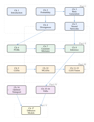
This book is organised into five parts, progressing from mathematical foundations to state-of-the-art generative models. fig:roadmap shows the dependency structure between chapters.

Part I - Foundations (Chapters 1–5)

We review the mathematical prerequisites: probability theory and statistics (Chapter 2), basic generation techniques such as rejection sampling and MCMC (Chapter 3), divergence measures including KL divergence and $f$-divergences (Chapter 4), and neural network architectures (Chapter 5).

Part II - Probabilistic Generative Models (Chapters 6–8)

We introduce probabilistic graphical models (Chapter 6), study Gaussian mixture models as a canonical example of latent-variable models (Chapter 7), and develop approximate inference techniques including expectation–maximisation and variational inference (Chapter 8).

Part III - Generative Adversarial Networks (Chapters 9–13)

We derive the GAN objective from first principles (Chapter 9), address training instabilities through Wasserstein GANs (Chapter 10), and survey GAN architectures for vision tasks (Chapters 11–13).

Part IV - Variational and Transport Methods (Chapters 14–16)

We study optimal transport and Sinkhorn distances (Chapter 14), then develop the VAE framework in depth across two chapters (Chapters 15–16), connecting variational inference with amortised optimisation.

Part V - Diffusion Models (Chapter 17)

We present denoising diffusion probabilistic models (DDPMs), connecting them to hierarchical VAEs, score matching, and stochastic differential equations.

Appendices

The appendices collect background material on real analysis (measure theory, convergence) and convex analysis (convex functions, duality, Fenchel conjugates) that is referenced throughout the main text.

Exercises