2 Probability and Statistics

Generative modelling is, at its mathematical core, the study of probability distributions. Every generative model, whether a Gaussian mixture, a variational autoencoder, or a diffusion model, is ultimately an attempt to represent, approximate, or sample from a probability distribution over high-dimensional data. This chapter reviews the probability and statistics needed to make that statement precise.

We assume the reader has encountered probability in an introductory course and focus on developing the concepts that will recur throughout the book. Readers comfortable with multivariate distributions, the change-of-variables formula, and maximum likelihood estimation may skim this chapter and return to it as a reference.

Random Variables and Distributions

Definition 1 (Random Variable).

A random variable $X$ is a measurable function from a sample space $Ω$ to the real numbers $ℝ$ . Informally, it assigns a numerical value to each outcome of a random experiment.

Random variables come in two flavours:

Discrete random variables take on a countable set of values (e.g., the number of heads in 10 coin tosses).
Continuous random variables take on values in an uncountable set, typically an interval of $ℝ$ (e.g., the intensity of a pixel in a photograph).

Probability Mass Functions

A discrete random variable $X$ is characterised by its probability mass function (PMF):

Definition 2 (Probability Mass Function).

The PMF of a discrete random variable $X$ is the function $p_{X} : ℝ \to [0,1]$ defined by $p_{X} (x) = P (X = x) .$ It satisfies $p_{X} (x) \geq 0$ for all $x$ and $\sum_{x} p_{X} (x) = 1$ .

Example 1 (Fair Die).

Rolling a fair six-sided die defines a random variable $X \in {1,2,3,4,5,6}$ with PMF $p_{X} (k) = \frac{1}{6}$ for each $k$ .

Probability Density Functions

A continuous random variable $X$ is characterised by its probability density function (PDF):

Definition 3 (Probability Density Function).

The PDF of a continuous random variable $X$ is a non-negative function $f_{X} : ℝ \to [0, \infty)$ such that for any interval $[a, b]$ , $P (a \leq X \leq b) = \int_{a}^{b} f_{X} (x) d x .$ The PDF satisfies $\int_{- \infty}^{\infty} f_{X} (x) d x = 1$ .

Remark 1.

A common source of confusion: $f_{X} (x)$ is not a probability. It is a probability density; it can exceed 1. Only the integral of $f_{X}$ over an interval gives a probability. For instance, a uniform distribution on $[0, 0.5]$ has $f_{X} (x) = 2$ for $x \in [0, 0.5]$ .

Cumulative Distribution Functions

Definition 4 (Cumulative Distribution Function).

The cumulative distribution function (CDF) of a random variable $X$ is $F_{X} (x) = P (X \leq x) .$ For continuous random variables, $F_{X} (x) = \int_{- \infty}^{x} f_{X} (t) d t$ , so $f_{X} (x) = F_{X}^{'} (x)$ .

Common Discrete Distributions

Bernoulli Distribution

The simplest random experiment has two outcomes: success (1) or failure (0).

Definition 5 (Bernoulli Distribution).

A random variable $X$ follows a Bernoulli distribution with parameter $p \in [0,1]$ , written $X \sim Bernoulli (p)$ , if $P (X = 1) = p, P (X = 0) = 1 - p .$

Insight.

A single pixel in a binary (black-and-white) image can be modelled as a Bernoulli random variable. A generative model for binary images assigns a Bernoulli parameter $p_{i} \in [0,1]$ to each pixel $i$ ; this is exactly what the output layer of a VAE decoder does when generating binary MNIST digits.

Binomial Distribution

Definition 6 (Binomial Distribution).

If $X_{1}, \dots, X_{n} \overset{iid}{\sim} Bernoulli (p)$ , then $Y = \sum_{i = 1}^{n} X_{i} \sim Binomial (n, p)$ with PMF $P (Y = k) = (\binom{n}{k}) p^{k} {(1 - p)}^{n - k}, k = 0, 1, \dots, n .$

Geometric Distribution

Definition 7 (Geometric Distribution).

A random variable $X \sim Geometric (p)$ models the number of trials until the first success: $P (X = k) = {(1 - p)}^{k - 1} p, k = 1, 2, 3, \dots$ The geometric distribution is the only discrete distribution with the memoryless property: $P (X > s + t | X > s) = P (X > t)$ .

Poisson Distribution

Definition 8 (Poisson Distribution).

A random variable $X \sim Poisson (λ)$ with rate parameter $λ > 0$ has PMF $P (X = k) = \frac{λ^{k} e^{- λ}}{k!}, k = 0, 1, 2, \dots$ It models the number of events occurring in a fixed interval of time or space, given a constant average rate $λ$ .

Example 2 (Word Counts).

The number of times a particular word appears in a document of fixed length can be modelled as a Poisson random variable. Topic models and language models use this observation to build generative models of text.

Categorical and Multinomial Distributions

Definition 9 (Categorical Distribution).

A random variable $X$ taking values in ${1, 2, \dots, K}$ follows a categorical distribution with parameters $𝝅 = (π_{1}, \dots, π_{K})$ , where $π_{k} \geq 0$ and $\sum_{k = 1}^{K} π_{k} = 1$ , if $P (X = k) = π_{k}$ .

Definition 10 (Multinomial Distribution).

If $X_{1}, \dots, X_{n}$ are i.i.d. $Categorical (𝝅)$ , the vector of counts $𝐍 = (N_{1}, \dots, N_{K})$ where $N_{k} = # {i : X_{i} = k}$ follows a multinomial distribution: $P (N_{1} = n_{1}, \dots, N_{K} = n_{K}) = \frac{n!}{n_{1}! \dots n_{K}!} π_{1}^{n_{1}} \dots π_{K}^{n_{K}},$ where $n = n_{1} + \dots + n_{K}$ .

Insight.

The categorical distribution is the workhorse of autoregressive language models. When GPT generates the next word (token), it produces a categorical distribution over a vocabulary of $K \approx 50,000$ tokens. Sampling from this distribution gives the next word. The entire generative process is a sequence of categorical samples, one per token.

Common Continuous Distributions

Uniform Distribution

Definition 11 (Uniform Distribution).

A random variable $X \sim Uniform (a, b)$ has PDF $f_{X} (x) = {\begin{matrix} \frac{1}{b - a} & if a \leq x \leq b, \\ 0 & otherwise. \end{matrix}$

The uniform distribution serves as the “noise source” in many generative models: to sample from a complex distribution, we often start with uniform (or Gaussian) random numbers and transform them.

Gaussian (Normal) Distribution

The Gaussian distribution is the single most important distribution in generative modelling. It appears as the noise prior in GANs, VAEs, normalizing flows, and diffusion models; it defines the likelihood in Gaussian mixture models; and it is the stationary distribution of many stochastic processes.

Definition 12 (Gaussian Distribution).

A random variable $X \sim 𝒩 (μ, σ^{2})$ has PDF $f_{X} (x) = \frac{1}{σ \sqrt{2 π}} \exp (- \frac{{(x - μ)}^{2}}{2 σ^{2}}),$ where $μ \in ℝ$ is the mean and $σ^{2} > 0$ is the variance.

Gaussian probability density functions with different means and variances. Changing

μ

shifts the curve; changing

σ^{2}

controls its width.

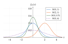
The Gaussian distribution owes its ubiquity to several remarkable properties:

It is the maximum entropy distribution among all distributions with a given mean and variance: it makes the fewest assumptions beyond these two moments.
Sums of independent random variables converge to a Gaussian (Central Limit Theorem).
It is closed under linear transformations, marginalisation, and conditioning.
Its log-density is quadratic, making optimisation tractable.

Exponential Distribution

Definition 13 (Exponential Distribution).

A random variable $X \sim Exponential (λ)$ with rate $λ > 0$ has PDF $f_{X} (x) = λ e^{- λ x}, x \geq 0.$ It is the continuous analogue of the geometric distribution and models waiting times.

Beta Distribution

Definition 14 (Beta Distribution).

A random variable $X \sim Beta (α, β)$ with shape parameters $α, β > 0$ has PDF $f_{X} (x) = \frac{x^{α - 1} {(1 - x)}^{β - 1}}{B (α, β)}, x \in [0, 1],$ where $B (α, β) = \frac{Γ (α) Γ (β)}{Γ (α + β)}$ is the Beta function.

The Beta distribution is the conjugate prior for the Bernoulli parameter $p$ , making it central to Bayesian inference (see Bayesian Inference). It can model any shape on $[0,1]$ : uniform ( $α = β = 1$ ), U-shaped ( $α = β < 1$ ), or peaked ( $α = β > 1$ ).

Expectation, Variance, and Moments

Expectation

Definition 15 (Expectation).

The expectation (or mean) of a random variable $X$ is $𝔼 [X] = {\begin{matrix} \sum_{x} x p_{X} (x) & (discrete), \\ \int_{- \infty}^{\infty} x f_{X} (x) d x & (continuous) . \end{matrix}$ More generally, for any function $g$ , $𝔼 [g (X)] = \sum_{x} g (x) p_{X} (x)$ or $\int g (x) f_{X} (x) d x$ .

Key properties. Expectation is linear: for any constants $a, b$ and random variables $X, Y$ , $𝔼 [a X + b Y] = a 𝔼 [X] + b 𝔼 [Y] .$ This holds even when $X$ and $Y$ are not independent.

Variance and Standard Deviation

Definition 16 (Variance).

The variance of a random variable $X$ with mean $μ = 𝔼 [X]$ is $𝖵ar (X) = 𝔼 [(X - μ)^{2}] = 𝔼 [X^{2}] - (𝔼 [X])^{2} .$ The standard deviation is $σ = \sqrt{𝖵ar (X)}$ .

Key properties. For constants $a, b$ : $𝖵ar (a X + b) = a^{2} 𝖵ar (X)$ . For independent $X, Y$ : $𝖵ar (X + Y) = 𝖵ar (X) + 𝖵ar (Y)$ .

Covariance and Correlation

Definition 17 (Covariance and Correlation).

The covariance of random variables $X$ and $Y$ is $𝖢ov (X, Y) = 𝔼 [(X - 𝔼 [X]) (Y - 𝔼 [Y])] = 𝔼 [X Y] - 𝔼 [X] 𝔼 [Y] .$ The correlation coefficient normalises covariance to $[- 1, 1]$ : $ρ (X, Y) = \frac{𝖢ov (X, Y)}{\sqrt{𝖵ar (X) 𝖵ar (Y)}} .$ If $X$ and $Y$ are independent, then $𝖢ov (X, Y) = 0$ . The converse is not generally true.

Remark 2.

For a random vector $𝐗 = {(X_{1}, \dots, X_{d})}^{⊤}$ , the covariance matrix is the $d \times d$ matrix $𝚺 = 𝔼 [(𝐗 - 𝝁) (𝐗 - 𝝁)^{⊤}], [𝚺]_{i j} = 𝖢ov (X_{i}, X_{j}) .$ This matrix encodes the variance of each component (on the diagonal) and the pairwise correlations (off-diagonal). It is symmetric and positive semi-definite. The covariance matrix is a central object in this book: it defines the shape of Gaussian distributions, appears in the FID metric, and governs the geometry of latent spaces.

Moments and Moment Generating Functions

Definition 18 (Moments).

The $k$ -th moment of $X$ is $𝔼 [X^{k}]$ . The $k$ -th central moment is $𝔼 [{(X - μ)}^{k}]$ . The first moment is the mean; the second central moment is the variance.

Definition 19 (Moment Generating Function).

The moment generating function (MGF) of $X$ is $M_{X} (t) = 𝔼 [e^{t X}],$ provided the expectation exists in a neighbourhood of $t = 0$ . The $k$ -th moment can be recovered as $𝔼 [X^{k}] = M_{X}^{(k)} (0)$ . If two random variables have the same MGF, they have the same distribution.

Joint, Marginal, and Conditional Distributions

When modelling data, we almost always deal with multiple random variables simultaneously. An image has millions of pixel values; a sentence has dozens of token indices. Understanding the relationships between these variables requires joint, marginal, and conditional distributions.

Joint Distributions

Definition 20 (Joint Distribution).

For continuous random variables $X$ and $Y$ , the joint PDF $f_{X, Y} (x, y)$ satisfies $P ((X, Y) \in A) = \iint_{A} f_{X, Y} (x, y) d x d y$ for any region $A \subseteq ℝ^{2}$ , and $\int \int f_{X, Y} (x, y) d x d y = 1$ .

Marginal Distributions

Given the joint distribution of $(X, Y)$ , we can recover the distribution of $X$ alone by marginalising out $Y$ : $f_{X} (x) = \int_{- \infty}^{\infty} f_{X, Y} (x, y) d y .$ For discrete variables, replace the integral with a sum.

Key Idea.

Marginalisation is one of the most important operations in generative modelling. When we write the marginal likelihood of a latent-variable model as $p_{θ} (𝐱) = \int p_{θ} (𝐱 | 𝐳) p (𝐳) d 𝐳,$ we are marginalising out the latent variable $𝐳$ to obtain the distribution over observed data $𝐱$ . The intractability of this integral for complex models is the central challenge that variational inference and VAEs are designed to address.

Conditional Distributions

Definition 21 (Conditional Distribution).

The conditional PDF of $Y$ given $X = x$ is $f_{Y | X} (y | x) = \frac{f_{X, Y} (x, y)}{f_{X} (x)}, provided f_{X} (x) > 0.$

Rearranging gives the product rule: $f_{X, Y} (x, y) = f_{Y | X} (y | x) \cdot f_{X} (x)$ . Applying this repeatedly to a vector $𝐱 = (x_{1}, \dots, x_{d})$ yields the chain rule of probability: (Chain RULE) $\begin{matrix} p (𝐱) = p (x_{1}) p (x_{2} | x_{1}) p (x_{3} | x_{1}, x_{2}) \dots p (x_{d} | x_{1}, \dots, x_{d - 1}) = \prod_{i = 1}^{d} p (x_{i} | x_{< i}) . \end{matrix}$ This decomposition is exact: no approximation is involved, and it is the foundation of autoregressive generative models (PixelCNN, GPT, WaveNet).

Independence

Definition 22 (Independence).

Random variables $X$ and $Y$ are independent if and only if $f_{X, Y} (x, y) = f_{X} (x) \cdot f_{Y} (y) for all x, y .$ Equivalently, $f_{Y | X} (y | x) = f_{Y} (y)$ : knowing $X$ tells you nothing about $Y$ .

Independence is a very strong assumption. In an image, pixels are not independent; neighbouring pixels are highly correlated. The gap between the independent (factored) model and the true joint distribution is precisely what generative models must learn to bridge.

Bayes' Theorem

Theorem 1 (Bayes' Theorem).

For continuous random variables $X$ and $Y$ with $f_{Y} (y) > 0$ , $f_{X | Y} (x | y) = \frac{f_{Y | X} (y | x) f_{X} (x)}{f_{Y} (y)} = \frac{f_{Y | X} (y | x) f_{X} (x)}{\int f_{Y | X} (y | x^{'}) f_{X} (x^{'}) d x^{'}} .$

In the language of Bayesian inference: $\underset{posterior}{\underset{⏟}{f_{X | Y} (x | y)}} = \frac{\overset{likelihood}{\overset{⏞}{f_{Y | X} (y | x)}} \cdot \overset{prior}{\overset{⏞}{f_{X} (x)}}}{\underset{evidence}{\underset{⏟}{f_{Y} (y)}}} .$ The denominator $f_{Y} (y) = \int f_{Y | X} (y | x) f_{X} (x) d x$ is a normalising constant that ensures the posterior integrates to 1. Computing this integral is often intractable, motivating the approximate inference methods developed in Chapter 8.

The Multivariate Gaussian Distribution

The multivariate Gaussian is the cornerstone of probabilistic generative modelling. It parameterises the prior in VAEs, defines the likelihood in Gaussian mixture models, serves as the base distribution in normalizing flows, and governs the noise process in diffusion models. We develop its properties in detail.

Definition 23 (Multivariate Gaussian Distribution).

A random vector $𝐱 \in ℝ^{d}$ follows a multivariate Gaussian (or normal) distribution, written $𝐱 \sim 𝒩 (𝝁, 𝚺)$ , if its PDF is (MVN PDF) $\begin{matrix} f (𝐱) = \frac{1}{{(2 π)}^{d / 2} | 𝚺 |^{1 / 2}} \exp (- \frac{1}{2} {(𝐱 - 𝝁)}^{⊤} 𝚺^{- 1} (𝐱 - 𝝁)), \end{matrix}$ where $𝝁 \in ℝ^{d}$ is the mean vector and $𝚺 \in ℝ^{d \times d}$ is a symmetric positive definite covariance matrix.

Contour lines of bivariate Gaussian distributions. Left:

𝚺 = 𝐈

gives circular contours (uncorrelated, equal variance in all directions). Right: off-diagonal entries produce tilted ellipses whose axes align with the eigenvectors of

𝚺

. The shape and orientation of the ellipses are entirely determined by the covariance matrix.

Geometry of the Multivariate Gaussian

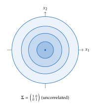
The exponent ${(𝐱 - 𝝁)}^{⊤} 𝚺^{- 1} (𝐱 - 𝝁)$ is the Mahalanobis distance from $𝐱$ to $𝝁$ , measured in the metric defined by $𝚺^{- 1}$ . The level sets of the density are ellipsoids centred at $𝝁$ :

The axes of the ellipsoid are aligned with the eigenvectors of $𝚺$ .
The lengths of the axes are proportional to the square roots of the eigenvalues.
If $𝚺 = σ^{2} 𝐈$ (all eigenvalues equal), the ellipsoid becomes a sphere, and the distribution is isotropic.

Marginals and Conditionals of a Gaussian

One of the most remarkable properties of the multivariate Gaussian is that both marginals and conditionals are again Gaussian. Partition $𝐱 = (\begin{matrix} 𝐱_{1} \\ 𝐱_{2} \end{matrix})$ with corresponding partition of the mean and covariance: $𝝁 = (\begin{matrix} 𝝁_{1} \\ 𝝁_{2} \end{matrix}), 𝚺 = (\begin{matrix} 𝚺_{11} & 𝚺_{12} \\ 𝚺_{21} & 𝚺_{22} \end{matrix}) .$

Proposition 1 (Marginal of a Gaussian).

The marginal distribution of $𝐱_{1}$ is $𝐱_{1} \sim 𝒩 (𝝁_{1}, 𝚺_{11}) .$

Proposition 2 (Conditional of a Gaussian).

The conditional distribution of $𝐱_{1}$ given $𝐱_{2} = 𝐚$ is $𝐱_{1} | 𝐱_{2} = 𝐚 \sim 𝒩 (𝝁_{1} + 𝚺_{12} 𝚺_{22}^{- 1} (𝐚 - 𝝁_{2}), 𝚺_{11} - 𝚺_{12} 𝚺_{22}^{- 1} 𝚺_{21}) .$

Insight.

These formulas have a beautiful interpretation. The conditional mean $𝝁_{1} + 𝚺_{12} 𝚺_{22}^{- 1} (𝐚 - 𝝁_{2})$ is the best linear prediction of $𝐱_{1}$ given $𝐱_{2} = 𝐚$ : it shifts the prior mean by an amount proportional to how much $𝐱_{2}$ deviates from its own mean. The conditional covariance $𝚺_{11} - 𝚺_{12} 𝚺_{22}^{- 1} 𝚺_{21}$ (the Schur complement) is always smaller than the marginal covariance $𝚺_{11}$ : observing $𝐱_{2}$ always reduces our uncertainty about $𝐱_{1}$ .

This property is used extensively in Gaussian processes, Kalman filters, and the derivation of the ELBO for linear Gaussian models.

Linear Transformations

Proposition 3 (Affine Transformation of a Gaussian).

If $𝐱 \sim 𝒩 (𝝁, 𝚺)$ and $𝐲 = 𝐀 𝐱 + 𝐛$ for a matrix $𝐀 \in ℝ^{m \times d}$ and vector $𝐛 \in ℝ^{m}$ , then $𝐲 \sim 𝒩 (𝐀 𝝁 + 𝐛, 𝐀 𝚺 𝐀^{⊤}) .$

Remark 3.

This closure under affine transformations is one reason why the standard Gaussian $𝒩 (𝟎, 𝐈)$ is the default choice for the latent prior in generative models: any Gaussian can be obtained from $𝐳 \sim 𝒩 (𝟎, 𝐈)$ via the transformation $𝐱 = 𝝁 + 𝐋 𝐳$ , where $𝚺 = 𝐋 𝐋^{⊤}$ (Cholesky decomposition). This is the basis of the reparameterisation trick used in VAE training.

Fundamental Theorems and Inequalities

Law of Large Numbers

Theorem 2 (Weak Law of Large Numbers).

Let $X_{1}, X_{2}, \dots, X_{n}$ be i.i.d. random variables with mean $μ$ and finite variance $σ^{2}$ . Then the sample mean $X_{n} = \frac{1}{n} \sum_{i = 1}^{n} X_{i}$ converges to $μ$ in probability: $\lim_{n \to \infty} P (| X_{n} - μ | \geq ϵ) = 0, \forall ϵ > 0.$

Proof.

By Chebyshev's inequality (Theorem 5 below), $P (| X_{n} - μ | \geq ϵ) \leq \frac{𝖵ar (X_{n})}{ϵ^{2}} = \frac{σ^{2}}{n ϵ^{2}} \overset{\overset{}{n \to \infty}}{\to} 0.$

∎

Key Idea.

The Law of Large Numbers justifies Monte Carlo estimation: we can approximate $𝔼 [g (X)]$ by averaging $g (X_{i})$ over i.i.d. samples. This is how we estimate the ELBO in VAE training and the adversarial loss in GAN training, by averaging over minibatches.

Central Limit Theorem

Theorem 3 (Central Limit Theorem).

Let $X_{1}, X_{2}, \dots, X_{n}$ be i.i.d. with mean $μ$ and finite variance $σ^{2} > 0$ . Then the standardised sum converges in distribution to a standard Gaussian: $Z_{n} = \frac{\sum_{i = 1}^{n} X_{i} - n μ}{σ \sqrt{n}} \overset{\overset{}{d}}{\to} 𝒩 (0, 1) as n \to \infty .$

The CLT explains why the Gaussian appears so frequently in nature and in modelling: whenever a quantity is the result of many small, independent contributions, its distribution is approximately Gaussian.

Concentration Inequalities

The following inequalities provide non-asymptotic bounds on how random variables deviate from their expectations.

Theorem 4 (Markov's Inequality).

For any non-negative random variable $X$ and $a > 0$ , $P (X \geq a) \leq \frac{𝔼 [X]}{a} .$

Theorem 5 (Chebyshev's Inequality).

For any random variable $X$ with mean $μ$ and variance $σ^{2}$ , and any $k > 0$ , $P (| X - μ | \geq k σ) \leq \frac{1}{k^{2}} .$

Proof.

Apply Markov's inequality to the non-negative random variable ${(X - μ)}^{2}$ with threshold $a = k^{2} σ^{2}$ : $P (| X - μ | \geq k σ) = P ({(X - μ)}^{2} \geq k^{2} σ^{2}) \leq \frac{𝔼 [{(X - μ)}^{2}]}{k^{2} σ^{2}} = \frac{σ^{2}}{k^{2} σ^{2}} = \frac{1}{k^{2}} .$

∎

Theorem 6 (Jensen's Inequality).

If $φ$ is a convex function and $X$ is a random variable with finite expectation, then $φ (𝔼 [X]) \leq 𝔼 [φ (X)] .$ If $φ$ is concave, the inequality reverses.

Insight.

Jensen's inequality is the mathematical engine behind the ELBO. Since $\log$ is concave, Jensen gives $\log 𝔼 [f (X)] \geq 𝔼 [\log f (X)]$ . Applied to the marginal likelihood $\log p (𝐱) = \log 𝔼_{p (𝐳)} [p (𝐱 | 𝐳)]$ , this yields a tractable lower bound, the starting point for variational inference. We will derive this in detail in Chapter 8.

Theorem 7 (Cauchy–Schwarz Inequality).

For any random variables $X$ and $Y$ with finite second moments, $| 𝔼 [X Y] |^{2} \leq 𝔼 [X^{2}] \cdot 𝔼 [Y^{2}] .$ Equivalently, $| 𝖢ov (X, Y) |^{2} \leq 𝖵ar (X) \cdot 𝖵ar (Y)$ , which shows that $| ρ (X, Y) | \leq 1$ .

Theorem 8 (Union Bound).

For any events $A_{1}, A_{2}, \dots, A_{n}$ , $P (⋃_{i = 1}^{n} A_{i}) \leq \sum_{i = 1}^{n} P (A_{i}) .$

Change of Variables

The change-of-variables formula tells us how a probability distribution transforms under a mapping. This is one of the most important technical tools in this book: it is the mathematical foundation of normalizing flows and appears in the derivation of many other generative models.

Univariate Case

Theorem 9 (Change of Variables - Univariate).

Let $X$ be a continuous random variable with PDF $f_{X} (x)$ , and let $Y = g (X)$ where $g$ is a strictly monotone, differentiable function. Then the PDF of $Y$ is $f_{Y} (y) = f_{X} (g^{- 1} (y)) \cdot | \frac{d}{d y} g^{- 1} (y) | .$

The factor $| (d / d y) g^{- 1} (y) |$ accounts for how $g$ stretches or compresses the probability mass. If $g$ expands a region, the density must decrease to keep the total probability equal to 1.

Example 3 (Log-Normal Distribution).

Let $X \sim 𝒩 (μ, σ^{2})$ and $Y = e^{X}$ . Since $g^{- 1} (y) = \ln y$ and $| d g^{- 1} / d y | = 1 / y$ , we get $f_{Y} (y) = \frac{1}{y σ \sqrt{2 π}} \exp (- \frac{{(\ln y - μ)}^{2}}{2 σ^{2}}), y > 0.$ This is the log-normal distribution.

Non-Injective Transformations

When $g$ is not one-to-one (e.g., $Y = X^{2}$ ), multiple values of $X$ map to the same $Y$ . We sum over all pre-images: $f_{Y} (y) = \sum_{{x : g (x) = y}} f_{X} (x) \cdot | \frac{d g_{i}^{- 1}}{d y} |,$ where the sum ranges over all branches of the inverse.

Example 4 (Chi-Squared from Standard Normal).

If $X \sim 𝒩 (0,1)$ and $Y = X^{2}$ , both $x = \sqrt{y}$ and $x = - \sqrt{y}$ map to $y$ . Each branch contributes $| d / d y | = 1 / (2 \sqrt{y})$ , giving $f_{Y} (y) = \frac{1}{\sqrt{2 π y}} e^{- y / 2}, y > 0,$ which is the $χ^{2} (1)$ distribution.

Multivariate Case

Theorem 10 (Change of Variables - Multivariate).

Let $𝐱 \in ℝ^{d}$ have density $f_{𝐱} (𝐱)$ , and let $𝐲 = 𝐠 (𝐱)$ where $𝐠 : ℝ^{d} \to ℝ^{d}$ is a differentiable bijection. Then (COV Multivariate) $\begin{matrix} f_{𝐲} (𝐲) = f_{𝐱} (𝐠^{- 1} (𝐲)) \cdot | \det \frac{\partial 𝐠^{- 1}}{\partial 𝐲} | = f_{𝐱} (𝐠^{- 1} (𝐲)) \cdot | \det 𝐉_{𝐠^{- 1}} (𝐲) |, \end{matrix}$ where $𝐉_{𝐠^{- 1}}$ is the Jacobian matrix of $𝐠^{- 1}$ .

Key Idea.

The multivariate change-of-variables formula is the mathematical heart of normalizing flows. A normalizing flow defines an invertible neural network $𝐠_{θ} : ℝ^{d} \to ℝ^{d}$ and uses (COV Multivariate) to compute the exact likelihood of any data point $𝐲$ : $\log p_{θ} (𝐲) = \log p_{𝐳} (𝐠_{θ}^{- 1} (𝐲)) + \log | \det 𝐉_{𝐠_{θ}^{- 1}} (𝐲) | .$ The challenge is designing architectures where both $𝐠_{θ}^{- 1}$ and its Jacobian determinant are efficient to compute. We will explore this in detail in the normalizing flows chapter.

Statistical Estimation

Having developed the probabilistic tools, we now turn to the question: given observed data, how do we estimate the parameters of a distribution? This is the problem that training a generative model must solve.

Point Estimation: Bias, Variance, and Consistency

Definition 24 (Estimator, Bias, and MSE).

An estimator ${\hat{θ}}_{n}$ of a parameter $θ$ is a function of the observed data $X_{1}, \dots, X_{n}$ .

The bias is $B ({\hat{θ}}_{n}) = 𝔼 [{\hat{θ}}_{n}] - θ$ . If $B = 0$ , the estimator is unbiased.
The mean squared error is $MSE ({\hat{θ}}_{n}) = 𝔼 [{({\hat{θ}}_{n} - θ)}^{2}] = 𝖵ar ({\hat{θ}}_{n}) + B {({\hat{θ}}_{n})}^{2}$ .

Definition 25 (Consistent Estimator).

An estimator ${\hat{θ}}_{n}$ is consistent if ${\hat{θ}}_{n} \overset{\overset{}{P}}{\to} θ$ as $n \to \infty$ , i.e., $\lim_{n \to \infty} P (| {\hat{θ}}_{n} - θ | \geq ϵ) = 0 \forall ϵ > 0.$

Proposition 4.

If $\lim_{n \to \infty} MSE ({\hat{θ}}_{n}) = 0$ , then ${\hat{θ}}_{n}$ is consistent.

Proof.

By Markov's inequality, $P (| {\hat{θ}}_{n} - θ | \geq ϵ) = P (| {\hat{θ}}_{n} - θ |^{2} \geq ϵ^{2}) \leq MSE ({\hat{θ}}_{n}) / ϵ^{2} \to 0$ .

∎

Maximum Likelihood Estimation

Definition 26 (Maximum Likelihood Estimator).

Given i.i.d. observations $x_{1}, \dots, x_{n}$ from a distribution $p_{θ}$ , the likelihood function is $L (θ) = \prod_{i = 1}^{n} p_{θ} (x_{i}) .$ The log-likelihood is $ℓ (θ) = \sum_{i = 1}^{n} \log p_{θ} (x_{i})$ . The maximum likelihood estimator (MLE) is ${\hat{θ}}_{MLE} = {arg max}_{θ} ℓ (θ) .$

Example 5 (MLE for a Gaussian).

Let $x_{1}, \dots, x_{n} \overset{iid}{\sim} 𝒩 (μ, σ^{2})$ . The log-likelihood is $ℓ (μ, σ^{2}) = - \frac{n}{2} \log (2 π σ^{2}) - \frac{1}{2 σ^{2}} \sum_{i = 1}^{n} {(x_{i} - μ)}^{2} .$ Setting derivatives to zero gives the MLEs: ${\hat{μ}}_{MLE} = \frac{1}{n} \sum_{i = 1}^{n} x_{i} = \overline{x}, {\hat{σ}}_{MLE}^{2} = \frac{1}{n} \sum_{i = 1}^{n} {(x_{i} - \overline{x})}^{2} .$ The mean estimator is unbiased; the variance estimator has bias $- σ^{2} / n$ (dividing by $n - 1$ instead of $n$ gives the unbiased version).

Key Idea.

Training a generative model by maximum likelihood is conceptually simple: we choose the parameters $θ$ that make the observed training data most probable under the model. In practice, the log-likelihood is averaged over minibatches and optimised with stochastic gradient descent: $θ \leftarrow θ + η \cdot \frac{1}{| ℬ |} \sum_{i \in ℬ} \nabla_{θ} \log p_{θ} (x_{i}) .$ This is the training procedure for autoregressive models, normalizing flows, and (with modifications) for VAEs and diffusion models.

Bayesian Inference

While MLE gives a single “best” parameter value, Bayesian inference maintains a full distribution over parameters, incorporating prior knowledge and quantifying uncertainty.

The setup: we have a prior $p (θ)$ expressing our beliefs before seeing data, and a likelihood $p (𝐱 | θ)$ . After observing data $𝐱$ , Bayes' theorem gives the posterior: $p (θ | 𝐱) = \frac{p (𝐱 | θ) p (θ)}{p (𝐱)}, p (𝐱) = \int p (𝐱 | θ) p (θ) d θ .$

Definition 27 (MAP Estimation).

The maximum a posteriori (MAP) estimate is the mode of the posterior: ${\hat{θ}}_{MAP} = {arg max}_{θ} p (θ | 𝐱) = {arg max}_{θ} [\log p (𝐱 | θ) + \log p (θ)] .$

Comparing with MLE: ${\hat{θ}}_{MAP} = {arg max}_{θ} [ℓ (θ) + \log p (θ)]$ . The prior $\log p (θ)$ acts as a regulariser. For example, a Gaussian prior $θ \sim 𝒩 (0, σ_{0}^{2})$ adds an $L_{2}$ penalty $- ‖ θ ‖^{2} / (2 σ_{0}^{2})$ , which is precisely weight decay in neural network training.

Example 6 (Conjugate Bayesian Inference for a Bernoulli).

Suppose we observe $k$ successes in $n$ Bernoulli trials and use a $Beta (α, β)$ prior on the success probability $p$ . The posterior is $p | data \sim Beta (α + k, β + n - k) .$ This is a conjugate update: the posterior is in the same family as the prior. As $n \to \infty$ , the posterior concentrates around the MLE $\hat{p} = k / n$ , and the prior becomes irrelevant. As $α, β \to 0$ , the MAP estimate approaches the MLE.

Remark 4.

The intractability of the posterior $p (θ | 𝐱)$ for complex models (deep neural networks have millions of parameters) is a central challenge in Bayesian deep learning. Variational inference, which we will develop in Chapter 8, approximates the posterior with a simpler distribution by minimising the KL divergence between them.

Exercises

Exercise 1.

Let $X$ be a discrete random variable taking values in ${1,2,3,4,5}$ with $P (X = k) = k / 15$ for $k = 1, \dots, 5$ . Compute the expectation $𝔼 [X]$ and the variance $𝖵ar (X)$ .

Exercise 2.

A medical test for a rare disease has a sensitivity (true positive rate) of 0.95 and a specificity (true negative rate) of 0.90. The prevalence of the disease is 0.01.

Using Bayes' theorem, compute the probability that a person who tests positive actually has the disease.
Interpret your result. Why is the positive predictive value so low despite the test's high sensitivity?
How does this relate to the challenge of evaluating generative models? Hint: think about the base rate of “real” vs. “generated” images in a dataset.

Exercise 3.

Let $X_{1}, \dots, X_{n} \overset{iid}{\sim} Bernoulli (p)$ .

Derive the maximum likelihood estimator ${\hat{p}}_{MLE}$ .
Show that ${\hat{p}}_{MLE}$ is unbiased.
Show that ${\hat{p}}_{MLE}$ is consistent.

Exercise 4.

Let $X$ and $Y$ have joint PDF $f_{X, Y} (x, y) = 6 (1 - y)$ for $0 \leq x \leq y \leq 1$ and $0$ otherwise.

Compute the marginal PDFs $f_{X} (x)$ and $f_{Y} (y)$ .
Compute the conditional PDF $f_{X | Y} (x | y)$ .
Are $X$ and $Y$ independent? Justify your answer.

Exercise 5.

Derive Chebyshev's inequality from Markov's inequality by applying Markov's inequality to the random variable ${(X - μ)}^{2}$ .

Exercise 6.

Let $x_{1}, \dots, x_{n} \overset{iid}{\sim} 𝒩 (μ, σ^{2})$ with both $μ$ and $σ^{2}$ unknown.

Derive the MLEs $\hat{μ}$ and ${\hat{σ}}^{2}$ .
Show that ${\hat{σ}}_{MLE}^{2}$ is biased and compute its bias.
Propose an unbiased estimator of $σ^{2}$ .

Exercise 7.

Let $X \sim 𝒩 (0,1)$ and $Y = X^{2}$ . Use the change-of-variables formula for non-injective transformations to derive the PDF of $Y$ . Identify the resulting distribution by name.

Exercise 8.

Let $X$ have prior $X \sim 𝒩 (μ_{0}, σ_{0}^{2})$ , and suppose we observe $Y = X + W$ where $W \sim 𝒩 (0, σ_{W}^{2})$ is independent of $X$ .

Show that the posterior $X | Y = y$ is Gaussian and find its mean and variance.
Derive the MAP estimate ${\hat{x}}_{MAP}$ and express it as a weighted average of $μ_{0}$ and $y$ .
What happens as $σ_{0}^{2} \to \infty$ ? Interpret this limit.
What happens as $σ_{W}^{2} \to 0$ ? Interpret this limit.

Exercise 9.

Let $𝐱 = {(X_{1}, X_{2})}^{⊤} \sim 𝒩 ((\begin{matrix} 0 \\ 0 \end{matrix}), (\begin{matrix} 4 & 2 \\ 2 & 3 \end{matrix}))$ .

Find the marginal distributions of $X_{1}$ and $X_{2}$ .
Find the conditional distribution of $X_{1} | X_{2} = 1$ .
Verify that the conditional variance is less than the marginal variance.

Exercise 10.

Let $𝐳 \sim 𝒩 (𝟎, 𝐈_{2})$ and define $𝐱 = 𝐠 (𝐳)$ where $𝐠 (z_{1}, z_{2}) = (z_{1}, z_{2} + z_{1}^{2})$ .

Show that $𝐠$ is invertible and find $𝐠^{- 1}$ .
Compute the Jacobian matrix $𝐉_{𝐠^{- 1}} (𝐱)$ and its determinant.
Write the density $f_{𝐱} (𝐱)$ using the change-of-variables formula.
Is $f_{𝐱}$ a Gaussian distribution? Why or why not?

This exercise illustrates how a normalizing flow can transform a simple Gaussian into a non-Gaussian distribution using an invertible mapping.

Exercise 11.

Let $X$ be a positive random variable.

Using Jensen's inequality with $φ = \log$ (a concave function), show that $𝔼 [\log X] \leq \log 𝔼 [X]$ .
Now let $p (𝐱, 𝐳) = p (𝐱 | 𝐳) p (𝐳)$ be a joint distribution and let $q (𝐳)$ be any distribution over $𝐳$ . Show that $\log p (𝐱) \geq 𝔼_{q (𝐳)} [\log \frac{p (𝐱, 𝐳)}{q (𝐳)}] .$ This inequality is the evidence lower bound (ELBO), the foundation of variational inference.

← 1 Introduction 3 Foundations of Generative Modelling →