3 Foundations of Generative Modelling
What does it mean for a machine to generate data? Consider the task of producing a new face photograph that looks realistic but does not depict any real person, or synthesising a plausible completion of a half-written paragraph. In each case, we want to draw a fresh sample from some complex, high-dimensional distribution (the distribution of natural face images, or of coherent English text) even though we only have access to a finite collection of examples from that distribution.
This chapter formalises the generative modelling problem and develops the core ideas that every later chapter builds on. We start from the simplest possible setting, sampling from a known one-dimensional distribution, and progressively introduce the key abstractions: push-forward maps, latent variables, and the reparameterisation trick. Along the way, we connect each idea to the concrete generative model families studied in Parts II–V of this book.
What Does “Generation” Mean?
Suppose we observe data drawn independently from an unknown distribution over a space (e.g. for images with pixels). The goal of generative modelling is to construct a mechanism that can produce new samples whose distribution closely approximates .
At first glance the problem sounds daunting: lives in high dimensions, is unknown, and may have a very complicated shape (multiple modes, thin ridges, etc.). Yet every approach we will study reduces the problem to two ingredients:
a source of randomness that is easy to sample (e.g. a standard Gaussian), and
a deterministic map that transforms simple noise into complex data.

The art lies in how we design and how we train it. Each family of generative models makes a different choice, as summarised in Table 1.
| Approach | How is trained | Chapters |
| Autoregressive models | Maximise via chain rule | 3, 6 |
| Normalising flows | Maximise via change of variables | 14 |
| VAEs | Maximise ELBO (lower bound on ) | 14 |
| GANs | Adversarial game (no explicit likelihood) | 9–13 |
| Diffusion models | Denoise score matching | 16 |
Remark 1 (Explicit vs. Implicit Models).
A model is called explicit (or prescribed) if it defines a density that can be evaluated, at least approximately. Autoregressive models, normalising flows, and VAEs are explicit. A model is implicit if it can produce samples but does not provide a tractable density. GANs are the prototypical implicit model.
Sampling from Known Distributions
Before tackling the full generative problem, we review how to sample from a known distribution. Every method rests on the same idea: transform uniform or Gaussian noise into the target distribution.
The Inverse-CDF Method
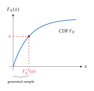
Let be a continuous random variable with cumulative distribution function . Because is monotonically non-decreasing and maps , we can (under mild regularity conditions) invert it.
Theorem 1 (Inverse-CDF Sampling).
Let . Define , where is the generalised inverse. Then .
Proof.
For any , where the second equality uses the monotonicity of and the third uses the fact that is uniform on .
Example 1 (Sampling from the Exponential Distribution).
Let , so for . Inverting gives . Hence, if , the transformation yields an exponential sample. In fact, since is also , we may simplify to .
Caution.
The inverse-CDF method requires that be available in closed form (or cheaply computable). For many distributions of interest, especially multivariate ones, this is not the case. That is precisely why we need more sophisticated methods.
The Box–Muller Transform
The Gaussian distribution does not have a closed-form inverse CDF. A classical workaround is the Box–Muller transform: given two independent uniform samples , define (BOX Muller) Then and are independent random variables.
Insight.
The Box–Muller transform is our first glimpse of a recurring theme: design a deterministic map that converts simple randomness into the distribution you want. Normalising flows (Chapter 14) generalise this idea by learning the map from data.
Rejection Sampling
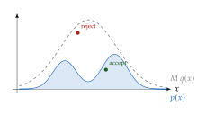
When neither the inverse CDF nor a clever transform is available, we can fall back on rejection sampling. Suppose we want to sample from a target density but can only evaluate it (up to a normalising constant). Choose a proposal density that is easy to sample and satisfies for some constant .
Algorithm 1 (Rejection Sampling).
Sample and .
If , accept ; otherwise reject and return to step 1.
The accepted samples are distributed exactly according to .
Proposition 1 (Correctness of Rejection Sampling).
Each accepted sample has density , and the acceptance probability is .
Proof.
The probability of accepting a proposal is . The marginal density of an accepted sample is The overall acceptance rate is .
Remark 2 (The Curse of Dimensionality in Rejection Sampling).
In high dimensions, the acceptance rate becomes astronomically small, and nearly all proposals are rejected. For instance, to sample a -dimensional standard Gaussian using a uniform proposal over a hypercube, the acceptance rate decays exponentially in . This is the fundamental reason why naive sampling methods fail for high-dimensional generative modelling, motivating the learned generators studied in later chapters.
Importance Sampling
Sometimes we do not need fresh samples but rather need to estimate an expectation when is hard to sample from. Importance sampling re-writes the expectation using a tractable proposal : (Importance Sampling) where are the importance weights.
Key Idea.
Importance sampling is not merely a computational trick; it is a cornerstone of variational inference (Chapter 8). The evidence lower bound (ELBO) used to train VAEs (Chapter 15) can be derived as an importance-weighted estimate of the log-marginal likelihood.
Maximum Likelihood Estimation for Generation
The simplest route to a generative model is: choose a parametric family , fit it to data by MLE, then sample from the fitted distribution.
Definition 1 (Maximum Likelihood Estimator).
Given i.i.d. observations , the maximum likelihood estimator (MLE) selects the parameter that maximises the likelihood: (MLE)
Once we have , generation is straightforward: sample .
Example 2 (Balls in a Bag: Bernoulli MLE).
Suppose a bag contains green and blue balls in unknown proportions. We draw balls with replacement and observe the sequence G, G, B, G, B, G (encoding Green = 1, Blue = 0). Model each draw as , where . The log-likelihood is Setting gives . To generate, we draw : each synthetic draw is Green with probability .
Example 3 (Fitting a Gaussian to Continuous Data).
Now consider continuous data: heights (in cm) of students: . Model them as . The MLE gives and . To generate a new “height”, sample , for example using the Box–Muller transform from The Box–Muller Transform.
Caution.
MLE with a simple parametric family (e.g. a single Gaussian) can only capture simple distributions. Natural images are not Gaussian; they live on a low-dimensional manifold within the high-dimensional pixel space. To model such distributions we need either (i) far richer parametric families (Gaussian mixtures, Chapter 7) or (ii) neural-network-based generators (Parts III–V).
Autoregressive Factorisation
For a -dimensional vector , the chain rule of probability gives an exact factorisation: (Chain RULE GEN) If each conditional is modelled by a parametric distribution (say a Gaussian or categorical) whose parameters are output by a neural network, we obtain an autoregressive model. Generation proceeds sequentially: sample , then given , and so on.
Insight.
Autoregressive models are the basis of modern large language models (GPT, LLaMA, etc.). Each token is generated by sampling from , which is exactly the chain-rule factorisation applied to sequences. The probabilistic graphical model view of this factorisation is studied in Chapter 6.
The Push-Forward Distribution
We now formalise the idea of “transforming noise into data.”
Definition 2 (Push-Forward Distribution).
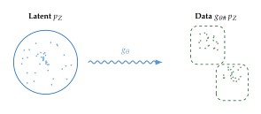
Let be a random variable with distribution on , and let be a measurable function. The push-forward of through , denoted , is the distribution of : Equivalently, for any test function ,
The push-forward viewpoint unifies all generative models:
Key Idea.
The generative modelling problem is to find a map such that . Different model families differ in how they parameterise (e.g. invertible network, decoder network, denoiser) and how they measure the approximation quality (e.g. KL divergence, Wasserstein distance, adversarial loss).
Connection to Change of Variables
When is a diffeomorphism (smooth, invertible, with smooth inverse), the push-forward density can be computed explicitly via the change-of-variables formula from Chapter 2: (PUSH Forward Density) This equation is the backbone of normalising flows: the generator is an invertible neural network, and the log-likelihood (NF Loglik) can be maximised exactly, with no approximations needed.
Remark 3 (When is Not Invertible).
If is not invertible (as in GANs and VAEs), we cannot use (PUSH Forward Density). Instead, the push-forward distribution is only defined implicitly through samples. For GANs this is fine, since the discriminator never needs to evaluate . For VAEs, the marginal likelihood is intractable, and we resort to variational bounds (Chapter 15).
The Generative Modelling Problem
We now state the central problem of this book precisely.
Definition 3 (The Generative Modelling Problem).
Let be observed data. Find a generator and a latent distribution on such that where the notion of “” is made precise by a discrepancy measure (e.g. KL divergence, Wasserstein distance, or an adversarial criterion): (GEN Problem) Common choices for include (Gaussian) and .
Remark 4 (Why the Discrepancy Matters).
The choice of profoundly affects the behaviour of the resulting model:
KL divergence leads to maximum likelihood training (Chapter 4).
Adversarial divergence yields GANs (Chapters 9–10).
Wasserstein distance gives Wasserstein GANs with better training stability (Chapter 10).
Score matching leads to diffusion models (Chapter 16).
Latent Variable Models
In practice, the data we observe (images, text, speech) lives in a very high-dimensional space, yet its intrinsic structure is often much lower-dimensional. Latent variable models make this explicit by introducing a hidden (latent) variable that “explains” the observations.
Definition 4 (Latent Variable Model).
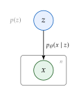
A latent variable model specifies:
a prior over latent codes , and
a likelihood (decoder) that generates an observation given a latent code.
The marginal (observed) distribution is obtained by integrating out : (Marginal Likelihood)
The Intractability Problem
The marginal likelihood involves an integral over the entire latent space, which is typically intractable: it cannot be computed in closed form when is parameterised by a neural network.
This intractability has two consequences:
We cannot evaluate exactly, so standard MLE is not directly applicable.
The posterior is also intractable, since it requires knowing .
Different model families deal with this in different ways:
| Model | Strategy for intractability |
| Normalising flows | Make invertible so the integral is not needed |
| VAEs | Introduce an approximate posterior and optimise a lower bound (ELBO) |
| GANs | Avoid computing entirely; use an adversarial discriminator instead |
| Diffusion models | Decompose generation into many small denoising steps, each tractable |
Insight.
Understanding why the marginal likelihood is intractable is the single most important conceptual step in generative modelling. Almost every architectural and algorithmic innovation you will encounter in Parts II–V is a creative response to this intractability.
The Reparameterisation Trick
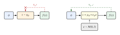
Suppose we want to optimise an objective that involves an expectation over a parameterised distribution. For instance, in a VAE the ELBO contains To perform gradient descent on , we need . But the sampling operation is not differentiable: how can we back-propagate through a random draw?
Definition 5 (Reparameterisation Trick).
Replace the parameterised sample with a deterministic transformation of parameter-free noise: (Reparam) where and are neural networks outputting the mean and standard deviation.
Now is a deterministic, differentiable function of (and ), so the gradient can be estimated by Monte Carlo and back-propagated through the network as usual.
Key Idea.
The reparameterisation trick is the key enabler of VAEs (Chapter 15) and also appears in the training of diffusion models (Chapter 16), where the noise added at each diffusion step is exactly the reparameterisation noise.
Evaluating Generative Models
How do we know whether a generative model produces “good” samples? This is surprisingly subtle; we need to assess both quality (do individual samples look realistic?) and diversity (does the model cover the full data distribution, or does it suffer from mode collapse?).
Definition 6 (Log-Likelihood).
For explicit models, the average test log-likelihood directly measures how well the model explains held-out data. Higher is better. This metric is not available for implicit models like GANs.
Definition 7 (Fréchet Inception Distance (FID)).
The FID [1] compares the statistics of real and generated images in the feature space of a pre-trained Inception network. Let and be the mean and covariance of Inception features for real and generated images, respectively. Then (FID) Lower FID indicates higher quality and diversity.
Remark 5 (Limitations of FID).
FID assumes that Inception features are Gaussian, a strong assumption. It also requires thousands of samples for a stable estimate. Nevertheless, FID remains the most widely used metric for image generation as of 2025.
Tractability and the Road Ahead
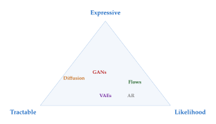
Let us take stock of the fundamental tension in generative modelling. We want a model that is simultaneously:
Expressive: capable of modelling complex, multimodal distributions in high dimensions.
Tractable: allowing efficient training and sampling.
Likelihood-evaluable: permitting computation of for evaluation and comparison.
No single model achieves all three perfectly. Figure 7 illustrates the trade-off.
The remainder of this book explores each major model family in depth:
Part II: Probabilistic Generative Models. Graphical models and Gaussian mixtures provide the classical foundation: exact inference is possible in small models, but approximate inference (EM, variational methods) is needed for larger ones.
Part III: Generative Adversarial Networks. GANs side-step likelihood computation entirely, using an adversarial game to train the generator. They excel at sample quality but can suffer from mode collapse and training instability.
Part IV: Variational and Transport Methods. VAEs and normalising flows provide principled likelihood-based training. VAEs use amortised variational inference; flows use invertible architectures for exact likelihood.
Part V: Diffusion Models. Diffusion models decompose the generation process into many small denoising steps, achieving state-of-the-art quality with stable training.
Each approach represents a different resolution of the expressiveness–tractability–likelihood triangle. The mathematical tools needed to understand these trade-offs (divergence measures, optimisation theory, and deep learning) are developed in the next two chapters.
Exercises
Exercise 1 (Inverse CDF for the Laplace Distribution).
The Laplace distribution with location and scale has CDF . Derive and describe how to generate Laplace samples from uniform random numbers.
Exercise 2 (Box–Muller Verification).
Starting from , use the change-of-variables formula (Chapter 2) to prove that and in (BOX Muller) are independent . Hint: first change to polar coordinates with and .
Exercise 3 (Rejection Sampling Efficiency).
Suppose the target is on and the proposal is . Find the smallest valid constant , describe the rejection criterion, and compute the acceptance rate.
Exercise 4 (Importance Sampling Variance).
Let and (indicator of a rare event). Compare the variance of estimating using (a) naïve Monte Carlo and (b) importance sampling with proposal . Which is more efficient and why?
Exercise 5 (MLE for a Gaussian Mixture).
Suppose the data is . Explain why a single Gaussian is a poor fit. What would be a better model? Write down the log-likelihood for a two-component Gaussian mixture model and explain why direct maximisation is difficult. (We will solve this properly in Chapter 7 using the EM algorithm.)
Exercise 6 (Push-Forward of a Linear Map).
Let and for invertible and . Use (PUSH Forward Density) to show that .
Exercise 7 (Can a Linear Generator Model a Mixture?).
Suppose and . Prove that no affine map can produce a push-forward . What does this imply about the expressiveness requirement for the generator?
Exercise 8 (Reparameterisation for the Exponential).
Show that if and , then . Write in the form for a deterministic function . Is differentiable with respect to ? Explain how this enables gradient-based optimisation of .
Exercise 9 (Intractable Marginal Likelihood).
Consider a latent variable model with and for learnable parameters . Write down the marginal likelihood . Explain why this integral has no closed-form solution. Suggest two strategies for training this model nonetheless.
Exercise 10 (Connecting the Three Approaches).
Explain how (a) inverse-CDF sampling, (b) MLE with a parametric family followed by sampling, and (c) the push-forward framework are related. In what sense are (a) and (b) special cases of the push-forward viewpoint? Give a concrete example where all three coincide.
Exercise 11 (FID in One Dimension (Computational)).
Suppose the “real” features are and the “generated” features are . Compute the FID using (FID) in one dimension (where the matrix square root reduces to the ordinary square root). What happens to the FID if the generated features are exactly?
References
-
Gans trained by a two time-scale update rule converge to a local nash equilibrium
BibTeX
@inproceedings{heusel2017gans, title={Gans trained by a two time-scale update rule converge to a local nash equilibrium}, author={Heusel, Martin and Ramsauer, Hubertus and Unterthiner, Thomas and Nessler, Bernhard and Hochreiter, Sepp}, booktitle={Advances in Neural Information Processing Systems}, pages={6626--6637}, year={2017} }Conference paper