19 Diffusion Models

Variational autoencoders, as developed in ch:vae,ch:vae2, learn a latent representation of data in a single encoding step. But what if we replaced that single step with a long chain of small, incremental corruptions, gradually transforming data into pure noise? This idea, rooted in non-equilibrium statistical physics, was first formalised by Sohl-Dickstein et al. [1] and later connected to variational inference by Ho et al. [2]. The result is a family of diffusion models that achieve remarkable sample quality by learning to reverse a carefully designed noise process. In this chapter we derive diffusion models as the natural limit of hierarchical VAEs, following the exposition of [5].

From Hierarchical VAEs to Diffusion Models

The standard VAE compresses an observation $x_{0}$ into a single latent code $𝒛$ and reconstructs from that code. A natural question is whether we can build a richer generative model by stacking multiple latent layers on top of one another, so that each layer captures progressively more abstract features. This is the idea behind hierarchical VAEs, and it turns out that diffusion models emerge as a special case when we push the hierarchy to its logical extreme.

Key Idea.

From VAEs to Hierarchical VAEs In ch:vae,ch:vae2 we built VAEs with a single latent layer: an encoder $q_{ϕ} (𝒛 | 𝒙)$ maps data to a latent code, and a decoder $p_{θ} (𝒙 | 𝒛)$ maps back. Hierarchical VAEs extend this by introducing a chain of latent variables $z_{1}, z_{2}, \dots, z_{T}$ , where each layer conditions on all previous layers. The encoder builds up a sequence of increasingly abstract representations, and the decoder reconstructs data by traversing the hierarchy in reverse.

Hierarchical VAE

Consider stacking multiple VAE layers into a fully connected directed acyclic graph (DAG), where each latent variable $z_{i}$ is conditioned on all preceding variables. The resulting graphical model has edges between every earlier node and every later node, as shown in fig:diff:hvae-dag.

Directed acyclic graph for a hierarchical VAE with fully connected dependencies. Each node

x_{i}

is conditioned on all preceding nodes.

A hierarchical VAE with both forward (black) and backward (red) processes. The observed variable

x_{1}

is drawn larger to distinguish it from the latent variables

z_{2}, \dots, z_{5}

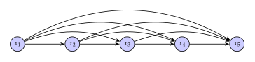
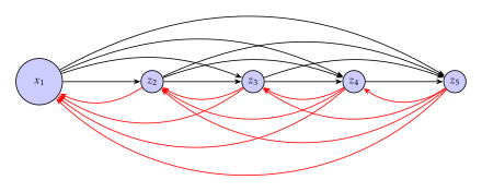
Let $pa (x_{i})$ denote the parents of $x_{i}$ in the DAG.\@ The joint distribution factorises according to the graph structure: $q (x_{1}, \dots, x_{D}) = \prod_{i = 1}^{D} q (x_{i} | pa (x_{i})) (forward process only)$

Applying the product rule explicitly, the forward joint distribution $q (x_{1}, \dots, z_{5})$ becomes $q (x_{1}, \dots, z_{5}) = q (x_{1}) q (z_{2} | x_{1}) q (z_{3} | x_{1}, z_{2}) q (z_{4} | x_{1}, z_{2}, z_{3}) q (z_{5} | x_{1}, z_{2}, z_{3}, z_{4}),$ where each latent variable $z_{i}$ is conditioned on all preceding variables. Similarly, the backward (generative) joint distribution factorises as $p (x_{1}, \dots, z_{5}) = p (z_{5}) p (z_{4} | z_{5}) p (z_{3} | z_{4}, z_{5}) p (z_{2} | z_{3}, z_{4}, z_{5}) p (x_{1} | z_{2}, z_{3}, z_{4}, z_{5}),$ where each variable is now conditioned on all subsequent variables.

This fully connected hierarchy captures all possible dependencies, but it raises a practical concern: with $T$ latent layers, each conditional depends on up to $T - 1$ variables. Can we simplify the model without losing too much expressive power?

The Markov Assumption

The fully connected hierarchical VAE requires each latent variable to condition on the entire history of preceding variables, making both inference and generation computationally expensive. A powerful simplification is to impose a Markov assumption: each variable depends only on its immediate predecessor. This reduces the graphical model from a fully connected DAG to a simple chain.

Graphical model for the Markovian forward process. Each node depends only on its immediate predecessor.

Graphical model for the Markovian backward (generative) process. Each node depends only on its immediate successor.

The Markovian VAE with both forward (top) and backward (bottom) transitions. A forward step from

z_{t - 1}

z_{t}

is governed by

q_{ϕ} (z_{t} | z_{t - 1})

, and the corresponding backward step is

p_{θ} (z_{t - 1} | z_{t})

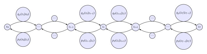
Under the Markov assumption, the joint distribution simplifies dramatically: $\begin{matrix} p (x, z_{1 : T}) & = p (z_{T}) p_{θ} (x_{0} | z_{1}) \prod_{t = 2}^{T} p_{θ} (z_{t - 1} | z_{t}) . \end{matrix}$ Note that this generative model proceeds from $z_{T}$ to $x_{0}$ , with each transition depending only on the immediately preceding latent variable. The posterior distribution (denoting $x_{0}$ as generic $x$ ) factorises as $\begin{matrix} q_{ϕ} (z_{1 : T} | x) & = q_{ϕ} (z_{1} | x) \prod_{t = 2}^{T} q_{ϕ} (z_{t} | z_{t - 1}) . \end{matrix}$

The ELBO for this Markovian hierarchical VAE follows the same derivation as in 15: $\begin{matrix} \log p (x) & = \log \int p (x, z_{1 : T}) d z_{1 : T} (Obtain likelihood; integrate out z) \\ = \log \int \frac{p (x, z_{1 : T})}{q_{ϕ} (z_{1 : T} | x)} q_{ϕ} (z_{1 : T} | x) d z_{1 : T} (multiply and divide by q_{ϕ}) \\ = \log 𝔼_{q_{ϕ} (z_{1 : T} | x)} [\frac{p (x, z_{1 : T})}{q_{ϕ} (z_{1 : T} | x)}] (write as expectation of q_{ϕ}) \\ \geq 𝔼_{q_{ϕ} (z_{1 : T} | x)} [\log \frac{p (x, z_{1 : T})}{q_{ϕ} (z_{1 : T} | x)}] (Jensen inequality) \end{matrix}$

Inserting the Markovian joint and posterior into the ELBO yields $\begin{matrix} 𝔼_{q_{ϕ} (z_{1 : T} | x)} [\log \frac{p (x, z_{1 : T})}{q_{ϕ} (z_{1 : T} | x)}] = 𝔼_{q_{ϕ} (z_{1 : T} | x)} [\log \frac{p (z_{T}) p_{θ} (x_{0} | z_{1}) \prod_{t = 2}^{T} p_{θ} (z_{t - 1} | z_{t})}{q_{ϕ} (z_{1} | x) \prod_{t = 2}^{T} q_{ϕ} (z_{t} | z_{t - 1})}] . \end{matrix}$

Historical Note.

The Thermodynamic Origins of Diffusion Sohl-Dickstein et al. [1] first proposed using diffusion processes from non-equilibrium thermodynamics as a foundation for generative modelling. The key insight was that if one can define a tractable process that gradually destroys structure in data, one can train a model to reverse this destruction. Five years later, Ho et al. [2] showed that this framework, when combined with a simplified training objective and careful noise scheduling, produces image samples rivalling those of GANs.

The Variational Diffusion Model

The Markovian VAE of the previous section still uses learned encoders $q_{ϕ} (z_{t} | z_{t - 1})$ with latent dimensions potentially smaller than the data dimension. The variational diffusion model (VDM) makes three key simplifications that transform this architecture into a diffusion model.

Key Idea.

Three Simplifications from MVAE to VDM

The latent dimension equals the data dimension: $\dim (x_{t}) = \dim (x_{0})$ for all $t$ .
The encoder $q (x_{t} | x_{t - 1})$ is not learned; it is a fixed linear Gaussian.
The Gaussian parameters are chosen so that $q (x_{T} | x_{0}) \approx 𝒩 (0, I)$ .

The variational diffusion model. Compared to the Markovian VAE in fig:diff:mvae-full, all latent variables

z_{t}

have been replaced by

x_{t}

(same dimensionality as

x_{0}

), and the forward encoder

q

is no longer parameterised.

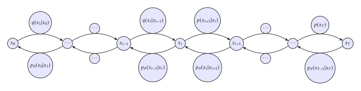
Notice in fig:diff:vdm that every latent variable is now denoted $x_{t}$ rather than $z_{t}$ , reflecting the fact that latent and data spaces share the same dimensionality. The forward encoder $q$ has no trainable parameters; only the backward decoder $p_{θ}$ is learned. With these changes, the posterior distribution becomes $\begin{matrix} q (x_{1 : T} | x_{0}) = \prod_{t = 1}^{T} q (x_{t} | x_{t - 1}) . \end{matrix}$

The Forward Process

Since the encoder is not learned, we must specify its form explicitly. The idea is to add a small amount of Gaussian noise at each step, with the noise level controlled by a variance schedule ${α_{t}}_{t = 1}^{T}$ .

Definition 1 (Forward Process).

The forward process defines each transition as a linear Gaussian: (Forward) $\begin{matrix} q (x_{t} | x_{t - 1}) = 𝒩 (x_{t}; \sqrt{α_{t}} x_{t - 1}, (1 - α_{t}) I), \end{matrix}$ where $α_{t} \in (0,1)$ for each $t = 1, \dots, T$ . The full forward posterior factorises as $\begin{matrix} q (x_{1 : T} | x_{0}) = \prod_{t = 1}^{T} q (x_{t} | x_{t - 1}) . \end{matrix}$ At each step, the mean shrinks the previous sample by $\sqrt{α_{t}}$ and adds Gaussian noise with variance $(1 - α_{t})$ . By choosing the schedule ${α_{t}}$ appropriately, the distribution $q (x_{T} | x_{0})$ converges to $𝒩 (0, I)$ for large $T$ .

ELBO for the Variational Diffusion Model

We now derive the evidence lower bound for the VDM.\@ The derivation follows the same Jensen's inequality argument as in 15, but applied to the $T$ -step Markov chain.

$\begin{matrix} \log p (x) & = \log \int p (x_{0 : T}) d x_{1 : T} = \log \int \frac{p (x_{0 : T}) q (x_{1 : T} | x_{0})}{q (x_{1 : T} | x_{0})} d x_{1 : T} [multiply and divide by q] \\ = \log 𝔼_{q (x_{1 : T} | x_{0})} [\frac{p (x_{0 : T})}{q (x_{1 : T} | x_{0})}] \geq 𝔼_{q (x_{1 : T} | x_{0})} [\log \frac{p (x_{0 : T})}{q (x_{1 : T} | x_{0})}] [Jensen’s inequality] \\ = 𝔼_{q (x_{1 : T} | x_{0})} [\log \frac{p (x_{T}) \prod_{t = 1}^{T} p_{θ} (x_{t - 1} | x_{t})}{\prod_{t = 1}^{T} q (x_{t} | x_{t - 1})}] [definition of joint] \\ = 𝔼_{q (x_{1 : T} | x_{0})} [\log \frac{p (x_{T}) p_{θ} (x_{0} | x_{1}) \prod_{t = 2}^{T} p_{θ} (x_{t - 1} | x_{t})}{q (x_{T} | x_{T - 1}) \prod_{t = 1}^{T - 1} q (x_{t} | x_{t - 1})}] [separate terms] \\ = 𝔼_{q (x_{1 : T} | x_{0})} [\log \frac{p (x_{T}) p_{θ} (x_{0} | x_{1})}{q (x_{T} | x_{T - 1})} \prod_{t = 1}^{T - 1} \frac{p_{θ} (x_{t} | x_{t + 1})}{q (x_{t} | x_{t - 1})}] [combine products] \end{matrix}$ Continuing further, we split the logarithm and simplify the expectations: $\begin{matrix} \log p (x) & \geq 𝔼_{q (x_{1 : T} | x_{0})} [\log \frac{p (x_{T}) p_{θ} (x_{0} | x_{1})}{q (x_{T} | x_{T - 1})}] + \sum_{t = 1}^{T - 1} 𝔼_{q (x_{1 : T} | x_{0})} [\log \frac{p_{θ} (x_{t} | x_{t + 1})}{q (x_{t} | x_{t - 1})}] [split log] \\ = 𝔼_{q (x_{1 : T} | x_{0})} [\log p_{θ} (x_{0} | x_{1})] + 𝔼_{q (x_{1 : T} | x_{0})} [\log \frac{p (x_{T})}{q (x_{T} | x_{T - 1})}] + \sum_{t = 1}^{T - 1} 𝔼_{q (x_{1 : T} | x_{0})} [\log \frac{p_{θ} (x_{t} | x_{t + 1})}{q (x_{t} | x_{t - 1})}] \\ [Above, we split first log term in view of writing KL and reconstruction terms!] \\ = 𝔼_{q (x_{1} | x_{0})} [\log p_{θ} (x_{0} | x_{1})] + 𝔼_{q (x_{T - 1}, x_{T} | x_{0})} [\log \frac{p (x_{T})}{q (x_{T} | x_{T - 1})}] \\ + \sum_{t = 1}^{T - 1} 𝔼_{q (x_{t - 1}, x_{t}, x_{t + 1} | x_{0})} [\log \frac{p_{θ} (x_{t} | x_{t + 1})}{q (x_{t} | x_{t - 1})}] \end{matrix}$ In the last equality, we replaced the joint $q (x_{1 : T} | x_{0})$ by the marginals that each term actually depends on.

Theorem 1 (ELBO for VDM (First Form)).

$\begin{matrix} \log p (x) & \geq 𝔼_{q (x_{1} | x_{0})} [\log p_{θ} (x_{0} | x_{1})] - 𝔼_{q (x_{T - 1} | x_{0})} [D_{KL} (q (x_{T} | x_{T - 1}) | | p (x_{T}))] \\ - \sum_{t = 1}^{T - 1} 𝔼_{q (x_{t - 1}, x_{t + 1} | x_{0})} [D_{KL} (q (x_{t} | x_{t - 1}) | | p_{θ} (x_{t} | x_{t + 1}))] \end{matrix}$

Remark 1 (Interpretation of the Three ELBO Terms).

The three terms in Theorem 1 each have a clear interpretation:

Reconstruction term: $𝔼_{q (x_{1} | x_{0})} [\log p_{θ} (x_{0} | x_{1})]$ measures how well the decoder reconstructs $x_{0}$ from the first latent step $x_{1}$ . This term is analogous to the reconstruction term in the standard VAE ELBO.
Prior matching term: $𝔼_{q (x_{T - 1} | x_{0})} [D_{KL} (q (x_{T} | x_{T - 1}) ‖ p (x_{T}))]$ penalises deviations of the final noisy distribution from the Gaussian prior. This term has no trainable parameters and vanishes for sufficiently large $T$ , since $q (x_{T} | x_{0})$ converges to $𝒩 (0, I)$ by design.
Consistency term: $𝔼_{q (x_{t - 1}, x_{t + 1} | x_{0})} [D_{KL} (q (x_{t} | x_{t - 1}) ‖ p_{θ} (x_{t} | x_{t + 1}))]$ enforces that the learned backward transition $p_{θ}$ at each step is consistent with the forward transition $q$ .

Applying Bayes' rule yields the true posterior

q (x_{t - 1} | x_{t}, x_{0})

(red), which runs parallel to the learned denoiser

p_{θ} (x_{t - 1} | x_{t})

(black). Matching these two distributions resolves the computational difficulty of the consistency term.

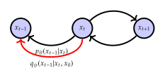
Remark 2 (Issues with the Consistency Term).

The consistency term $𝔼_{q (x_{t - 1}, x_{t + 1} | x_{0})} [D_{KL} (q (x_{t} | x_{t - 1}) ‖ p_{θ} (x_{t} | x_{t + 1}))]$ requires computing an expectation over the joint $q (x_{t - 1}, x_{t + 1} | x_{0})$ , which involves two correlated random variables. This is difficult to estimate efficiently. The remedy is to apply Bayes' rule: $\begin{matrix} q (x_{t} | x_{t - 1}, x_{0}) = \frac{q (x_{t - 1} | x_{t}, x_{0}) q (x_{t} | x_{0})}{q (x_{t - 1} | x_{0})} . \end{matrix}$ Note that we added $x_{0}$ as a condition, which is valid since $q (x_{t} | x_{t - 1}, x_{0}) = q (x_{t} | x_{t - 1})$ by the Markov property. As illustrated in fig:diff:bayes-consistency, this yields the true posterior $q (x_{t - 1} | x_{t}, x_{0})$ , which runs parallel to $p_{θ} (x_{t - 1} | x_{t})$ . Matching these two distributions will let us rewrite the ELBO in a more tractable form.

Revised ELBO via Bayes' Rule

We now rederive the ELBO, this time applying Bayes' rule to replace $q (x_{t} | x_{t - 1})$ with the tractable posterior $q (x_{t - 1} | x_{t}, x_{0})$ . Starting again from Jensen's inequality: (NEW ELBO LAST) $\begin{matrix} \log p (x) & \geq 𝔼_{q (x_{1 : T} | x_{0})} [\log \frac{p (x_{0 : T})}{q (x_{1 : T} | x_{0})}] \\ = 𝔼_{q (x_{1 : T} | x_{0})} [\log \frac{p (x_{T}) \prod_{t = 1}^{T} p_{θ} (x_{t - 1} | x_{t})}{\prod_{t = 1}^{T} q (x_{t} | x_{t - 1})}] \\ = 𝔼_{q (x_{1 : T} | x_{0})} [\log \frac{p (x_{T}) p_{θ} (x_{0} | x_{1}) \prod_{t = 2}^{T} p_{θ} (x_{t - 1} | x_{t})}{q (x_{1} | x_{0}) \prod_{t = 2}^{T} q (x_{t} | x_{t - 1})}] \\ = 𝔼_{q (x_{1 : T} | x_{0})} [\log \frac{p (x_{T}) p_{θ} (x_{0} | x_{1})}{q (x_{1} | x_{0})} \prod_{t = 2}^{T} \frac{p_{θ} (x_{t - 1} | x_{t})}{q (x_{t} | x_{t - 1}, x_{0})}] \\ = 𝔼_{q (x_{1 : T} | x_{0})} [\log \frac{p (x_{T}) p_{θ} (x_{0} | x_{1})}{q (x_{1} | x_{0})} + \log \prod_{t = 2}^{T} \frac{p_{θ} (x_{t - 1} | x_{t})}{q (x_{t} | x_{t - 1}, x_{0})}] \\ = 𝔼_{q (x_{1 : T} | x_{0})} [\log \frac{p (x_{T}) p_{θ} (x_{0} | x_{1})}{q (x_{1} | x_{0})} + \log \prod_{t = 2}^{T} \frac{p_{θ} (x_{t - 1} | x_{t})}{\frac{q (x_{t - 1} | x_{t}, x_{0}) q (x_{t} | x_{0})}{q (x_{t - 1} | x_{0})}}] \end{matrix}$ We now examine the product inside the last term. Separating it into two factors: $\begin{matrix} \prod_{t = 2}^{T} \frac{p_{θ} (x_{t - 1} | x_{t})}{\frac{q (x_{t - 1} | x_{t}, x_{0}) q (x_{t} | x_{0})}{q (x_{t - 1} | x_{0})}} & = \prod_{t = 2}^{T} \frac{p_{θ} (x_{t - 1} | x_{t})}{q (x_{t - 1} | x_{t}, x_{0})} \times \prod_{t = 2}^{T} \frac{q (x_{t - 1} | x_{0})}{q (x_{t} | x_{0})} \\ [Inner terms (Nr. and Dr.) of s e c o n d p r o d u c t gets canceled] \\ = \prod_{t = 2}^{T} \frac{p_{θ} (x_{t - 1} | x_{t})}{q (x_{t - 1} | x_{t}, x_{0})} \cdot \frac{q (x_{1} | x_{0})}{q (x_{T} | x_{0})} \end{matrix}$ The second product telescopes, leaving only the boundary terms. Substituting back into : $\begin{matrix} \log p (x) & \geq 𝔼_{q (x_{1 : T} | x_{0})} [\log \frac{p (x_{T}) p_{θ} (x_{0} | x_{1})}{q (x_{1} | x_{0})} + \log \frac{q (x_{1} | x_{0})}{q (x_{T} | x_{0})} + \log \prod_{t = 2}^{T} \frac{p_{θ} (x_{t - 1} | x_{t})}{q (x_{t - 1} | x_{t}, x_{0})}] (cancel r e d) \\ = 𝔼_{q (x_{1 : T} | x_{0})} [\log \frac{p (x_{T}) p_{θ} (x_{0} | x_{1})}{q (x_{T} | x_{0})} + \sum_{t = 2}^{T} \log \frac{p_{θ} (x_{t - 1} | x_{t})}{q (x_{t - 1} | x_{t}, x_{0})}] \\ = 𝔼_{q (x_{1 : T} | x_{0})} [\log p_{θ} (x_{0} | x_{1})] + 𝔼_{q (x_{1 : T} | x_{0})} [\log \frac{p (x_{T})}{q (x_{T} | x_{0})}] + \sum_{t = 2}^{T} 𝔼_{q (x_{1 : T} | x_{0})} [\log \frac{p_{θ} (x_{t - 1} | x_{t})}{q (x_{t - 1} | x_{t}, x_{0})}] \\ = 𝔼_{q (x_{1} | x_{0})} [\log p_{θ} (x_{0} | x_{1})] + 𝔼_{q (x_{T} | x_{0})} [\log \frac{p (x_{T})}{q (x_{T} | x_{0})}] + \sum_{t = 2}^{T} 𝔼_{q (x_{t}, x_{t - 1} | x_{0})} [\log \frac{p_{θ} (x_{t - 1} | x_{t})}{q (x_{t - 1} | x_{t}, x_{0})}] \\ = 𝔼_{q (x_{1} | x_{0})} [\log p_{θ} (x_{0} | x_{1})] - D_{KL} (q (x_{T} | x_{0}) | | p (x_{T})) \\ - \sum_{t = 2}^{T} 𝔼_{q (x_{t} | x_{0})} [D_{KL} (q (x_{t - 1} | x_{t}, x_{0}) | | p_{θ} (x_{t - 1} | x_{t}))] \end{matrix}$

Theorem 2 (ELBO for VDM (Revised Form)).

(ELBO Revised) $\begin{matrix} \log p (x) & \geq 𝔼_{q (x_{1} | x_{0})} [\log p_{θ} (x_{0} | x_{1})] - D_{KL} (q (x_{T} | x_{0}) | | p (x_{T})) \\ - \sum_{t = 2}^{T} 𝔼_{q (x_{t} | x_{0})} [D_{KL} (q (x_{t - 1} | x_{t}, x_{0}) | | p_{θ} (x_{t - 1} | x_{t}))] \end{matrix}$ The three terms have the following roles:

$𝔼_{q (x_{1} | x_{0})} [\log p_{θ} (x_{0} | x_{1})]$ is the reconstruction term, as before.
$D_{KL} (q (x_{T} | x_{0}) ‖ p (x_{T}))$ is the prior matching term: it compares the final noisy distribution to the standard Gaussian prior.
$𝔼_{q (x_{t} | x_{0})} [D_{KL} (q (x_{t - 1} | x_{t}, x_{0}) ‖ p_{θ} (x_{t - 1} | x_{t}))]$ is the denoising matching term: it measures how well the learned backward step $p_{θ}$ matches the true posterior $q (x_{t - 1} | x_{t}, x_{0})$ .

Marginal Distribution $q (x_{t} | x_{0})$

A crucial property of the linear Gaussian forward process is that we can compute the distribution of $x_{t}$ given $x_{0}$ in closed form, without iterating through all intermediate steps.

Theorem 3 (Marginal Distribution).

(Marginal) $\begin{matrix} q (x_{t} | x_{0}) = 𝒩 (x_{t}; \sqrt{{\overline{α}}_{t}} x_{0}, (1 - {\overline{α}}_{t}) I), where {\overline{α}}_{t} = \prod_{i = 1}^{t} α_{i} . \end{matrix}$

Proof.

$\begin{matrix} x_{t} & = \sqrt{α_{t}} x_{t - 1} + \sqrt{1 - α_{t}} ϵ_{t - 1}^{*}, (where ϵ_{t - 1}^{*} \sim 𝒩 (0, I)) \\ = \sqrt{α_{t}} (\sqrt{α_{t - 1}} x_{t - 2} + \sqrt{1 - α_{t - 1}} ϵ_{t - 2}^{*}) + \sqrt{1 - α_{t}} ϵ_{t - 1}^{*} (substitute x_{t - 1}) \\ = \sqrt{α_{t} α_{t - 1}} x_{t - 2} + \sqrt{α_{t} - α_{t} α_{t - 1}} ϵ_{t - 2}^{*} + \sqrt{1 - α_{t}} ϵ_{t - 1}^{*} \\ = \sqrt{α_{t} α_{t - 1}} x_{t - 2} + \sqrt{{\sqrt{α_{t} - α_{t} α_{t - 1}}}^{2} + {\sqrt{1 - α_{t}}}^{2}} ϵ_{t - 2} (used γ ϵ_{i} + ζ ϵ_{j} \sim N (0, γ^{2} + ζ^{2})) \\ = \sqrt{α_{t} α_{t - 1}} x_{t - 2} + \sqrt{α_{t} - α_{t} α_{t - 1} + 1 - α_{t}} ϵ_{t - 2} \\ = \sqrt{α_{t} α_{t - 1}} x_{t - 2} + \sqrt{1 - α_{t} α_{t - 1}} ϵ_{t - 2} (cancel α_{t}) \\ = \dots (continue recursion, simplification) \\ = (\sqrt{\prod_{i = 1}^{t} α_{i}}) x_{0} + (\sqrt{1 - \prod_{i = 1}^{t} α_{i}}) ϵ_{0} (after recursion) \\ = \sqrt{{\overline{α}}_{t}} x_{0} + \sqrt{1 - {\overline{α}}_{t}} ϵ_{0} (since \overline{α} = \prod_{i = 1}^{t} α_{i}) \\ \sim 𝒩 (x_{t}; \sqrt{{\overline{α}}_{t}} x_{0}, (1 - {\overline{α}}_{t}) I) (x_{0} constant ⟹ var (x_{0}) = 0, E [x_{0}] = x_{0}) . \end{matrix}$

∎

True Posterior $q (x_{t - 1} | x_{t}, x_{0})$

The revised ELBO in Theorem 2 requires the true denoising posterior $q (x_{t - 1} | x_{t}, x_{0})$ . We obtain it by applying Bayes' rule and completing the square in the exponent of the resulting Gaussian.

Theorem 4 (True Denoising Posterior).

$\begin{matrix} q (x_{t - 1} | x_{t}, x_{0}) & \propto 𝒩 (x_{t - 1}; \frac{\sqrt{α_{t}} (1 - α_{t - 1}) x_{t} + \sqrt{α_{t - 1}} (1 - α_{t}) x_{0}}{1 - {\overline{α}}_{t}}, \frac{(1 - α_{t}) (1 - α_{t - 1})}{1 - {\overline{α}}_{t}} I) \\ \propto 𝒩 (x_{t - 1}; μ_{q} (x_{t}, x_{0}), Σ_{q} (t)) \end{matrix}$

Proof.

We begin by applying Bayes' rule and substituting the known Gaussian forms from Definition 1 and Theorem 3: $\begin{matrix} q (x_{t - 1} | x_{t}, x_{0}) & = \frac{q (x_{t} | x_{t - 1}, x_{0}) q (x_{t - 1} | x_{0})}{q (x_{t} | x_{0})} \\ = \frac{𝒩 (x_{t}; \sqrt{α_{t}} x_{t - 1}, (1 - α_{t}) I) 𝒩 (x_{t - 1}; \sqrt{{\overline{α}}_{t - 1}} x_{0}, (1 - {\overline{α}}_{t - 1}) I)}{𝒩 (x_{t}; \sqrt{{\overline{α}}_{t}} x_{0}, (1 - {\overline{α}}_{t}) I)} \\ \propto \exp {- [\frac{{(x_{t} - \sqrt{α_{t}} x_{t - 1})}^{2}}{2 (1 - α_{t})} + \frac{{(x_{t - 1} - \sqrt{{\overline{α}}_{t - 1}} x_{0})}^{2}}{2 (1 - {\overline{α}}_{t - 1})} - \frac{{(x_{t} - \sqrt{{\overline{α}}_{t}} x_{0})}^{2}}{2 (1 - {\overline{α}}_{t})}]} \\ = \exp {- \frac{1}{2} [\frac{{(x_{t} - \sqrt{α_{t}} x_{t - 1})}^{2}}{1 - α_{t}} + \frac{{(x_{t - 1} - \sqrt{{\overline{α}}_{t - 1}} x_{0})}^{2}}{1 - {\overline{α}}_{t - 1}} - \frac{{(x_{t} - \sqrt{{\overline{α}}_{t}} x_{0})}^{2}}{1 - {\overline{α}}_{t}}]} \\ = \exp {- \frac{1}{2} [\frac{(- 2 \sqrt{α_{t}} x_{t} x_{t - 1} + α_{t} x_{t - 1}^{2})}{1 - α_{t}} + \frac{(x_{t - 1}^{2} - 2 \sqrt{{\overline{α}}_{t - 1}} x_{t - 1} x_{0})}{1 - {\overline{α}}_{t - 1}} + C (x_{t}, x_{0}))]} \\ \propto \exp {- \frac{1}{2} [\frac{- 2 \sqrt{α_{t}} x_{t} x_{t - 1}}{1 - α_{t}} + \frac{α_{t} x_{t - 1}^{2}}{1 - α_{t}} + \frac{x_{t - 1}^{2}}{1 - {\overline{α}}_{t - 1}} - \frac{2 \sqrt{{\overline{α}}_{t - 1}} x_{t - 1} x_{0}}{1 - {\overline{α}}_{t - 1}}]} \\ = \exp {- \frac{1}{2} [(\frac{α_{t}}{1 - α_{t}} + \frac{1}{1 - {\overline{α}}_{t - 1}}) x_{t - 1}^{2} - 2 (\frac{\sqrt{α_{t}} x_{t}}{1 - α_{t}} + \frac{\sqrt{{\overline{α}}_{t - 1}} x_{0}}{1 - {\overline{α}}_{t - 1}}) x_{t - 1}]} \end{matrix}$

∎

Remark 3 (The Constant $C (x_{t}, x_{0})$ ).

The constant term dropped in the proof above is (THE Constant) $\begin{matrix} C (x_{t}, x_{0}) = \frac{x_{t}^{2}}{1 - α_{t}} + \frac{{\overline{α}}_{t - 1} x_{0}^{2}}{1 - {\overline{α}}_{t - 1}} - \frac{(x_{t} - \sqrt{{\overline{α}}_{t}} x_{0})^{2}}{1 - {\overline{α}}_{t}} . \end{matrix}$ Since this term depends only on $x_{0}$ and $x_{t}$ , both of which are given as conditions, it is treated as a constant with respect to $x_{t - 1}$ . We will reintroduce $C$ when completing the square below.

Continuing the proof by simplifying the coefficient of $x_{t - 1}^{2}$ and completing the square: $\begin{matrix} q (x_{t - 1} | x_{t}, x_{0}) & = \exp {- \frac{1}{2} [\frac{α_{t} (1 - {\overline{α}}_{t - 1}) + 1 - α_{t}}{(1 - α_{t}) (1 - {\overline{α}}_{t - 1})} x_{t - 1}^{2} - 2 (\frac{\sqrt{α_{t}} x_{t}}{1 - α_{t}} + \frac{\sqrt{{\overline{α}}_{t - 1}} x_{0}}{1 - {\overline{α}}_{t - 1}}) x_{t - 1}]} \\ = \exp {- \frac{1}{2} [\frac{α_{t} - α_{t} + 1 - α_{t}}{(1 - α_{t}) (1 - α_{t - 1})} x_{t - 1}^{2} - 2 (\frac{\sqrt{α_{t}} x_{t}}{1 - α_{t}} + \frac{\sqrt{α_{t - 1}} x_{0}}{1 - α_{t - 1}}) x_{t - 1}]} \\ = \exp {- \frac{1}{2} [\frac{1 - α_{t}}{(1 - α_{t}) (1 - α_{t - 1})} x_{t - 1}^{2} - 2 (\frac{\sqrt{α_{t}} x_{t}}{1 - α_{t}} + \frac{\sqrt{α_{t - 1}} x_{0}}{1 - α_{t - 1}}) x_{t - 1}]} \\ = \exp {- \frac{1}{2} (\frac{1 - α_{t}}{(1 - α_{t}) (1 - α_{t - 1})}) [x_{t - 1}^{2} - 2 \frac{(\frac{\sqrt{α_{t}} x_{t}}{1 - α_{t}} + \frac{\sqrt{α_{t - 1}} x_{0}}{1 - α_{t - 1}})}{\frac{1 - α_{t}}{(1 - α_{t}) (1 - α_{t - 1})}} x_{t - 1}]} \\ = \exp {- \frac{1}{2} \frac{1 - α_{t}}{(1 - α_{t}) (1 - α_{t - 1})} [x_{t - 1}^{2} - 2 \frac{(\frac{\sqrt{α_{t}} x_{t}}{1 - α_{t}} + \frac{\sqrt{{\overline{α}}_{t - 1}} x_{0}}{1 - α_{t - 1}}) (1 - α_{t}) (1 - α_{t - 1})}{1 - {\overline{α}}_{t}} x_{t - 1}]} \\ = \exp {- \frac{1}{2} (\frac{1}{\frac{(1 - α_{t}) (1 - α_{t - 1})}{1 - α_{t}}}) [x_{t - 1}^{2} - 2 \frac{\sqrt{α_{t}} (1 - α_{t - 1}) x_{t} + \sqrt{α_{t - 1}} (1 - α_{t}) x_{0}}{1 - {\overline{α}}_{t}} x_{t - 1}]} \\ \propto 𝒩 (x_{t - 1}; \frac{\sqrt{α_{t}} (1 - α_{t - 1}) x_{t} + \sqrt{α_{t - 1}} (1 - α_{t}) x_{0}}{1 - {\overline{α}}_{t}}, \frac{(1 - α_{t}) (1 - α_{t - 1})}{1 - {\overline{α}}_{t}} I) \\ \propto 𝒩 (x_{t - 1}; μ_{q} (x_{t}, x_{0}), Σ_{q} (t)) . \end{matrix}$ This completes the proof. The constant $C (x_{t}, x_{0})$ that we dropped earlier is precisely the term needed to complete the square.

Remark 4 (Completing the Square).

To verify the final step, observe that (Complete Square) $\begin{matrix} q (x_{t - 1} | x_{t}, x_{0}) & = \exp {- \frac{1}{2} \frac{1 - α_{t}}{(1 - α_{t}) (1 - α_{t - 1})} \\ \times [x_{t - 1}^{2} - 2 \frac{\sqrt{α_{t}} (1 - α_{t - 1}) x_{t} + \sqrt{α_{t - 1}} (1 - α_{t}) x_{0}}{1 - {\overline{α}}_{t}} x_{t - 1}]} \\ \propto 𝒩 (x_{t - 1}; \frac{\sqrt{α_{t}} (1 - α_{t - 1}) x_{t} + \sqrt{α_{t - 1}} (1 - α_{t}) x_{0}}{1 - {\overline{α}}_{t}}, \frac{(1 - α_{t}) (1 - α_{t - 1})}{1 - {\overline{α}}_{t}} I) \\ \propto 𝒩 (x_{t - 1}; μ_{q} (x_{t}, x_{0}), Σ_{q} (t)) . \end{matrix}$ To prove , use the constant $C (x_{t}, x_{0})$ from to complete the square in : $\begin{matrix} (x_{t - 1} & - \frac{\sqrt{α_{t}} (1 - α_{t - 1}) x_{t} + \sqrt{α_{t - 1}} (1 - α_{t}) x_{0}}{1 - {\overline{α}}_{t}})^{2} \\ = x_{t - 1}^{2} - 2 \frac{\sqrt{α_{t}} (1 - α_{t - 1}) x_{t} + \sqrt{α_{t - 1}} (1 - α_{t}) x_{0}}{1 - {\overline{α}}_{t}} x_{t - 1} \\ + (\frac{1 - {\overline{α}}_{t}}{(1 - α_{t}) (1 - {\overline{α}}_{t - 1})})^{- 1} C (x_{t}, x_{0}) . \end{matrix}$

Remark 5 (Predetermined Variance).

Theorem 4 shows that at each step, $x_{t - 1}$ given $x_{t}$ and $x_{0}$ follows a Gaussian with mean $μ_{q} (x_{t}, x_{0})$ and variance $Σ_{q} (t)$ that is predetermined by the schedule ${α_{t}}$ . The variance depends only on $t$ , not on any trainable parameters. It can be written as $Σ_{q} (t) = σ_{q}^{2} (t) I$ , where (Sigma Q) $\begin{matrix} σ_{q}^{2} (t) = \frac{(1 - α_{t}) (1 - α_{t - 1})}{1 - α_{t}} . \end{matrix}$ The goal of training is therefore to align the approximate denoiser $p_{θ} (x_{t - 1} | x_{t})$ with the ground-truth posterior $q (x_{t - 1} | x_{t}, x_{0})$ . Since both distributions are Gaussian with the same variance, matching them reduces to matching their means.

The Denoising Objective

Now that both $q (x_{t - 1} | x_{t}, x_{0})$ and $p_{θ} (x_{t - 1} | x_{t})$ are Gaussian with identical variance $σ_{q}^{2} (t) I$ , the KL divergence between them simplifies to a function of their means alone.

Theorem 5 (KL Divergence between Gaussians).

The Kullback-Leibler divergence between two Gaussian distributions is $\begin{matrix} D_{KL} & (𝒩 (x; μ_{x}, Σ_{x}) ‖ 𝒩 (y; μ_{y}, Σ_{y})) \\ = \frac{1}{2} [\log \frac{| Σ_{y} |}{| Σ_{x} |} - d + tr (Σ_{y}^{- 1} Σ_{x}) + (μ_{y} - μ_{x})^{⊤} Σ_{y}^{- 1} (μ_{y} - μ_{x})] . \end{matrix}$

Theorem 6 (Denoising Matching Objective).

When $q$ and $p_{θ}$ share the same variance $σ_{q}^{2} (t) I$ , the denoising matching term reduces to $\begin{matrix} \arg \min_{θ} & D_{KL} (q (x_{t - 1} | x_{t}, x_{0}) ‖ p_{θ} (x_{t - 1} | x_{t})) \\ = \arg \min_{θ} \frac{1}{2 σ_{q}^{2} (t)} ‖ μ_{θ} - μ_{q} ‖_{2}^{2} \end{matrix}$

Proof.

$\begin{matrix} \arg \min_{θ} D_{KL} (q (x_{t - 1} | x_{t}, x_{0}) ‖ p_{θ} (x_{t - 1} | x_{t})) \\ = \arg \min_{θ} D_{KL} (𝒩 (x_{t - 1}; μ_{q}, Σ_{q} (t)) ‖ 𝒩 (x_{t - 1}; μ_{θ}, Σ_{q} (t))) \\ = \arg \min_{θ} \frac{1}{2} [\log \frac{| Σ_{q} (t) |}{| Σ_{q} (t) |} - d + tr (Σ_{q} (t)^{- 1} Σ_{q} (t)) \\ + (μ_{θ} - μ_{q})^{⊤} Σ_{q} (t)^{- 1} (μ_{θ} - μ_{q})] \\ = \arg \min_{θ} \frac{1}{2} [\log 1 - d + d + (μ_{θ} - μ_{q})^{⊤} Σ_{q} (t)^{- 1} (μ_{θ} - μ_{q})] \\ = \arg \min_{θ} \frac{1}{2} [(μ_{θ} - μ_{q})^{⊤} Σ_{q} (t)^{- 1} (μ_{θ} - μ_{q})] \\ = \arg \min_{θ} \frac{1}{2} [(μ_{θ} - μ_{q})^{⊤} (σ_{q}^{2} (t) I)^{- 1} (μ_{θ} - μ_{q})] \\ = \arg \min_{θ} \frac{1}{2} \frac{1}{σ_{q}^{2} (t)} ‖ μ_{θ} - μ_{q} ‖_{2}^{2} . \end{matrix}$

∎

Here $μ_{q}$ is shorthand for $μ_{q} (x_{t}, x_{0})$ and $μ_{θ}$ for $μ_{θ} (x_{t}, t)$ . The denoiser $p_{θ}$ must therefore learn to predict the mean of the true posterior $q$ .

The true mean is given by (Theorem 4):

Definition 2 (True Denoiser Mean).

$\begin{matrix} μ_{q} (x_{t}, x_{0}) = \frac{\sqrt{α_{t}} (1 - α_{t - 1}) x_{t} + \sqrt{α_{t - 1}} (1 - α_{t}) x_{0}}{1 - α_{t}} . \end{matrix}$

The approximate denoiser mirrors this formula but replaces the unknown $x_{0}$ with a learned estimate:

Definition 3 (Approximate Denoiser Mean).

The approximate denoiser uses the mean (Approx MEAN) $\begin{matrix} μ_{θ} (x_{t}, t) = \frac{\sqrt{α_{t}} (1 - α_{t - 1}) x_{t} + \sqrt{α_{t - 1}} (1 - α_{t}) {\hat{x}}_{θ} (x_{t}, t)}{1 - α_{t}}, \end{matrix}$ where ${\hat{x}}_{θ} (x_{t}, t)$ is a neural network that attempts to predict $x_{0}$ from the noisy observation $x_{t}$ at timestep $t$ .

Theorem 7 ( $x_{0}$ -Prediction Loss).

Given the true denoiser mean $μ_{q} (x_{t}, x_{0})$ and the approximate denoiser mean $μ_{θ} (x_{t}, t)$ as defined above, the denoising matching objective simplifies to $\begin{matrix} \arg \min_{θ} D_{KL} (q (x_{t - 1} | x_{t}, x_{0}) ‖ p_{θ} (x_{t - 1} | x_{t})) \\ = \arg \min_{θ} \frac{1}{2 σ_{q}^{2} (t)} (\frac{\sqrt{α_{t - 1}} (1 - α_{t})}{1 - α_{t}})^{2} ‖ ({\hat{x}}_{θ} (x_{t}, t) - x_{0}) ‖_{2}^{2} . \end{matrix}$

Proof.

$\begin{matrix} \arg \min_{θ} D_{KL} (q (x_{t - 1} | x_{t}, x_{0}) ‖ p_{θ} (x_{t - 1} | x_{t})) \\ = \arg \min_{θ} D_{KL} (𝒩 (x_{t - 1}; μ_{q}, Σ_{q} (t)) ‖ 𝒩 (x_{t - 1}; μ_{θ}, Σ_{q} (t))) \\ = \arg \min_{θ} \frac{1}{2 σ_{q}^{2} (t)} ‖ \frac{\sqrt{α_{t}} (1 - α_{t - 1}) x_{t} + \sqrt{α_{t - 1}} (1 - α_{t}) {\hat{x}}_{θ} (x_{t}, t)}{1 - {\overline{α}}_{t}} \\ - \frac{\sqrt{α_{t}} (1 - {\overline{α}}_{t - 1}) x_{t} + \sqrt{α_{t - 1}} (1 - α_{t}) x_{0}}{1 - {\overline{α}}_{t}} ‖_{2}^{2} \\ = \arg \min_{θ} \frac{1}{2 σ_{q}^{2} (t)} ‖ \frac{\sqrt{{\overline{α}}_{t - 1}} (1 - α_{t})}{1 - {\overline{α}}_{t}} {\hat{x}}_{θ} (x_{t}, t) - \frac{\sqrt{α_{t - 1}} (1 - α_{t})}{1 - α_{t}} x_{0} ‖_{2}^{2} \\ = \arg \min_{θ} \frac{1}{2 σ_{q}^{2} (t)} ‖ \frac{\sqrt{α_{t - 1}} (1 - α_{t})}{1 - α_{t}} ({\hat{x}}_{θ} (x_{t}, t) - x_{0}) ‖_{2}^{2} \\ = \arg \min_{θ} \frac{1}{2 σ_{q}^{2} (t)} (\frac{\sqrt{α_{t - 1}} (1 - α_{t})}{1 - α_{t}})^{2} ‖ ({\hat{x}}_{θ} (x_{t}, t) - x_{0}) ‖_{2}^{2} . \end{matrix}$

∎

Remark 6 (Interpretation of the $x_{0}$ -Prediction Loss).

Theorem 7 reveals that optimising the denoising matching term in the ELBO is equivalent to training a neural network ${\hat{x}}_{θ} (x_{t}, t)$ to predict the clean data $x_{0}$ from its noisy version $x_{t}$ . The time-dependent prefactor weights the loss differently at each noise level, but the core task is always the same: denoise. The model parameters $θ$ are learned by supervised regression against ground-truth clean samples.

DDPM: Training and Inference

The mathematical machinery of the previous section (the ELBO decomposition, the closed-form posterior, and the $x_{0}$ -prediction loss) remained largely theoretical until Ho et al. [2] crystallised them into a practical algorithm called the Denoising Diffusion Probabilistic Model (DDPM). Their key contribution was not a new derivation but a concrete recipe: a simple training loop, a matching sampling loop, and a set of design choices (noise schedule, network architecture, loss weighting) that together produce high-quality images rivalling GANs.

The DDPM Loss Function

Combining the per-timestep KL terms from Theorem 2 into a single objective yields the full DDPM loss. Because every term reduces to an $x_{0}$ -prediction mean-squared error (as shown in the previous section), the summation takes a clean and interpretable form.

Definition 4 (DDPM Loss).

The full DDPM loss sums over all timesteps. It is the negation of the denoising-matching contribution to the ELBO, so minimising it maximises the bound: $\begin{matrix} L (θ) & = \sum_{t = 1}^{T} 𝔼_{q (x_{t} | x_{0})} [\frac{1}{2 σ_{q}^{2} (t)} (\frac{{\overline{α}}_{t - 1} {(1 - α_{t})}^{2}}{{(1 - {\overline{α}}_{t})}^{2}}) {‖ {\hat{x}}_{θ} (x_{t}) - x_{0} ‖}^{2}] \\ = \sum_{t = 1}^{T} [\frac{1}{2 σ_{q}^{2} (t)} (\frac{{\overline{α}}_{t - 1} {(1 - α_{t})}^{2}}{{(1 - {\overline{α}}_{t})}^{2}}) 𝔼_{q (x_{t} | x_{0})} {‖ {\hat{x}}_{θ} (x_{t}) - x_{0} ‖}^{2}] . \end{matrix}$

Remark 7 (Interpretation of the Loss).

This formulation of the ELBO highlights several critical aspects:

Reconstruction error. Each term within the summation directly relates to the reconstruction error between the predicted data ${\hat{x}}_{θ} (x_{t})$ and the original data $x_{0}$ . This error is scaled inversely by the noise variance $σ_{q}^{2} (t)$ , which adjusts the impact of each timestep based on the model's noise schedule.
Noise schedule dependency. The noise schedule is explicitly integrated into the ELBO through the parameters $α_{t}$ and ${\overline{α}}_{t - 1}$ . The terms involving these parameters adjust how the model weights the importance of errors at different timesteps, effectively shaping the learning trajectory.
Linearity of expectation. The expectation operator is linear, allowing the external factors like the variance scaling and noise parameters to be handled outside of the expectation. This property simplifies the computation and interpretation of the ELBO, making it computationally feasible to handle within the stochastic gradient descent framework typically used to train such models.

In practice, the summation over all timesteps is replaced by an expectation over a uniformly sampled timestep $t \sim Uniform {1, \dots, T}$ , yielding a stochastic estimate of $L (θ)$ suitable for mini-batch gradient descent: $\begin{matrix} L (θ) & = T 𝔼_{t \sim U {1, T}} [\frac{1}{2 σ_{q}^{2} (t)} (\frac{{\overline{α}}_{t - 1} {(1 - α_{t})}^{2}}{{(1 - {\overline{α}}_{t})}^{2}}) 𝔼_{q (x_{t} | x_{0})} {‖ {\hat{x}}_{θ} (x_{t}) - x_{0} ‖}^{2}] . \end{matrix}$

Training Algorithm

The training procedure is pleasingly simple: sample a data point, pick a random timestep, corrupt the data with the corresponding noise level, and take a gradient step to make the network's prediction closer to the original clean data.

Algorithm 1 (DDPM Training).

Algorithm 1: DDPM Training [2].

[H]

repeat
Sample $x_{0} \sim p_{data}$
Sample $t \sim Uniform {1, \dots, T}$
Sample $ϵ \sim 𝒩 (0, I)$
$x_{t} \leftarrow \sqrt{{\overline{α}}_{t}} x_{0} + \sqrt{1 - {\overline{α}}_{t}} ϵ$
Take gradient step on $\nabla_{θ} ‖ {\hat{x}}_{θ} (x_{t}, t) - x_{0} ‖^{2}$
until converged

An important detail is the choice of ${\overline{α}}_{t}$ , the cumulative product of the variance reduction factors up to timestep $t$ . The selection of ${\overline{α}}_{t}$ affects the trajectory of the noise addition and must be carefully calibrated to balance learning efficiency and model stability. We return to this question in Learned Noise Schedules.

Sampling and Inference

After training, the model generates new data by reversing the diffusion process. Starting from pure Gaussian noise $x_{T} \sim 𝒩 (0, I)$ , we iteratively apply the learned reverse transition $\begin{matrix} x_{t - 1} \sim p_{θ} (x_{t - 1} | x_{t}) & = 𝒩 (x_{t - 1} | μ_{θ} (x_{t}), σ_{q}^{2} (t) I) \\ realised as x_{t - 1} = μ_{θ} (x_{t}) + σ_{q} (t) z, z \sim 𝒩 (0, I), \end{matrix}$ where the mean is given by $\begin{matrix} μ_{θ} (x_{t}) = \frac{(1 - {\overline{α}}_{t - 1}) \sqrt{α_{t}}}{1 - {\overline{α}}_{t}} x_{t} + \frac{(1 - α_{t}) \sqrt{{\overline{α}}_{t - 1}}}{1 - {\overline{α}}_{t}} {\hat{x}}_{θ} (x_{t}) . \end{matrix}$ At each step the network predicts a clean image ${\hat{x}}_{θ} (x_{t})$ , which is blended with the current noisy state $x_{t}$ to produce the mean of the reverse step. Stochasticity enters through the noise term $σ_{q} (t) z$ . At the final step ( $t = 1$ ) the noise is omitted, producing the deterministic output $x_{0}$ .

Algorithm 2 (DDPM Sampling).

Algorithm 2: DDPM Sampling [2].

[H]

Sample $x_{T} \sim 𝒩 (0, I)$
for $t = T, T - 1, \dots, 1$
$z \sim 𝒩 (0, I)$ if $t > 1$ , else $z = 0$
$x_{t - 1} \leftarrow \frac{(1 - {\overline{α}}_{t - 1}) \sqrt{α_{t}}}{1 - {\overline{α}}_{t}} x_{t} + \frac{(1 - α_{t}) \sqrt{{\overline{α}}_{t - 1}}}{1 - {\overline{α}}_{t}} {\hat{x}}_{θ} (x_{t}, t) + σ_{q} (t) z$
return $x_{0}$

Signal-to-Noise Ratio

A unifying lens through which to view the loss, the noise schedule, and the weighting of different timesteps is the signal-to-noise ratio (SNR). Recall that the forward process satisfies $q (x_{t} | x_{0}) = 𝒩 (x_{t}; \sqrt{{\overline{α}}_{t}} x_{0}, (1 - {\overline{α}}_{t}) I)$ . The mean carries the “signal” $\sqrt{{\overline{α}}_{t}} x_{0}$ and the variance carries the “noise” $(1 - {\overline{α}}_{t})$ .

Definition 5 (Signal-to-Noise Ratio).

For a Gaussian $𝒩 (μ, σ^{2} I)$ , the signal-to-noise ratio is $SNR = ‖ μ ‖^{2} / σ^{2}$ . Applied to the forward process $q (x_{t} | x_{0})$ , whose mean is $\sqrt{{\overline{α}}_{t}} x_{0}$ , this gives ${\overline{α}}_{t} ‖ x_{0} ‖^{2} / (1 - {\overline{α}}_{t})$ ; for unit-scaled data ( $‖ x_{0} ‖ = 1$ ) this is (SNR) $\begin{matrix} SNR (t) = \frac{{\overline{α}}_{t}}{1 - {\overline{α}}_{t}} . \end{matrix}$

The SNR starts high at $t = 0$ (mostly signal, little noise) and decreases monotonically toward zero as $t \to T$ (mostly noise, little signal). A good noise schedule ensures that $SNR (T) \approx 0$ , so that $x_{T}$ is nearly pure Gaussian noise, and that the decrease is smooth enough for the network to learn at every noise level.

Theorem 8 (Loss in Terms of SNR).

Proof.

$\begin{matrix} \frac{1}{2 σ_{q}^{2} (t)} \frac{{\overline{α}}_{t - 1} {(1 - α_{t})}^{2}}{{(1 - {\overline{α}}_{t})}^{2}} {‖ ({\hat{x}}_{θ} (x_{t}, t) - x_{0}) ‖}_{2}^{2} \\ = \frac{1}{\frac{2 (1 - α_{t}) (1 - {\overline{α}}_{t - 1})}{1 - {\overline{α}}_{t}}} \frac{{\overline{α}}_{t - 1} {(1 - α_{t})}^{2}}{{(1 - {\overline{α}}_{t})}^{2}} {‖ {\hat{x}}_{θ} (x_{t}, t) - x_{0} ‖}_{2}^{2} \\ = \frac{1}{2} \frac{1 - {\overline{α}}_{t}}{(1 - α_{t}) (1 - {\overline{α}}_{t - 1})} \frac{{\overline{α}}_{t - 1} {(1 - α_{t})}^{2}}{{(1 - {\overline{α}}_{t})}^{2}} {‖ ({\hat{x}}_{θ} (x_{t}, t) - x_{0}) ‖}_{2}^{2} \\ = \frac{1}{2} \frac{{\overline{α}}_{t - 1} (1 - α_{t})}{(1 - {\overline{α}}_{t - 1}) (1 - {\overline{α}}_{t})} {‖ ({\hat{x}}_{θ} (x_{t}, t) - x_{0}) ‖}_{2}^{2} \\ = \frac{1}{2} \frac{{\overline{α}}_{t - 1} - {\overline{α}}_{t} + {\overline{α}}_{t - 1} {\overline{α}}_{t} - {\overline{α}}_{t - 1} {\overline{α}}_{t}}{(1 - {\overline{α}}_{t - 1}) (1 - {\overline{α}}_{t})} {‖ {\hat{x}}_{θ} (x_{t}, t) - x_{0} ‖}_{2}^{2} \\ = \frac{1}{2} \frac{{\overline{α}}_{t - 1} (1 - {\overline{α}}_{t}) - {\overline{α}}_{t} (1 - {\overline{α}}_{t - 1})}{(1 - {\overline{α}}_{t - 1}) (1 - {\overline{α}}_{t})} {‖ {\hat{x}}_{θ} (x_{t}, t) - x_{0} ‖}_{2}^{2} \\ = \frac{1}{2} (\frac{{\overline{α}}_{t - 1} (1 - {\overline{α}}_{t})}{(1 - {\overline{α}}_{t - 1}) (1 - {\overline{α}}_{t})} - \frac{{\overline{α}}_{t} (1 - {\overline{α}}_{t - 1})}{(1 - {\overline{α}}_{t - 1}) (1 - {\overline{α}}_{t})}) {‖ ({\hat{x}}_{θ} (x_{t}, t) - x_{0}) ‖}_{2}^{2} \\ = \frac{1}{2} (\frac{{\overline{α}}_{t - 1}}{1 - {\overline{α}}_{t - 1}} - \frac{{\overline{α}}_{t}}{1 - {\overline{α}}_{t}}) {‖ ({\hat{x}}_{θ} (x_{t}, t) - x_{0}) ‖}_{2}^{2} . \end{matrix}$

∎

Theorem 8 tells us that the per-timestep loss can be written purely in terms of the SNR drop between consecutive timesteps. In particular, the differential SNR between two consecutive timesteps gives the per-step loss a transparent interpretation: (SNR TIME) $\begin{matrix} L_{t} (x) & = \frac{1}{2} (\frac{{\overline{α}}_{t - 1}}{1 - {\overline{α}}_{t - 1}} - \frac{{\overline{α}}_{t}}{1 - {\overline{α}}_{t}}) ‖ {\hat{x}}_{θ} (x_{t}, t) - x_{0} ‖_{2}^{2} \\ = \frac{1}{2} (SNR (t - 1) - SNR (t)) ‖ {\hat{x}}_{θ} (x_{t}, t) - x_{0} ‖_{2}^{2} . \end{matrix}$ Each term is the product of an SNR drop and the network's prediction error at that noise level. Timesteps where the SNR changes rapidly contribute more to the loss, while timesteps where the SNR is nearly constant contribute little. For the standard cosine and linear- $β$ schedules the drop is largest at small $t$ , so this weighting emphasises the low-noise end of the chain, which is one reason Ho et al. [2] found that discarding the weight altogether improves perceptual sample quality. Minimising $L_{t} (x)$ is thus synonymous with denoising: the model learns to reverse the noise added during the forward process, reconstructing $x_{0}$ from $x_{t}$ with increasing accuracy as training progresses.

Learned Noise Schedules

The noise schedule ${α_{t}}_{t = 1}^{T}$ (equivalently, the SNR schedule) is a design choice that profoundly affects sample quality. Two classical families are:

Variance preserving (VP) [1]: the forward process keeps the total variance of $x_{t}$ constant at every step; in the parameterisation of Definition 1 this means $α_{t} = 1 - σ_{t}^{2}$ , where $σ_{t}^{2}$ is the variance added at step $t$ .
Variance exploding (VE) [3]: the signal coefficient on $x_{0}$ is held at $1$ and only the noise variance grows over time, so $x_{t} = x_{0} + σ_{t} ϵ$ . This does not fit the $(\sqrt{α_{t}}, 1 - α_{t})$ parameterisation of Definition 1 directly; the two are related by the rescaling $x_{t}^{VE} = x_{t}^{VP} / \sqrt{{\overline{α}}_{t}}$ , which leaves the signal-to-noise ratio unchanged.

Rather than hand-crafting the schedule, Kingma et al. [4] proposed learning it end-to-end by parameterising the SNR directly with a monotonic neural network $ω_{η} (t)$ : (Learned SNR) $\begin{matrix} SNR (t) = \exp (- ω_{η} (t)), \end{matrix}$ where $ω_{η}$ is constrained to be monotonically increasing so that the SNR decreases with $t$ . From this parameterisation the cumulative signal coefficient follows immediately: (Alpha Sigmoid) $\begin{matrix} \frac{{\overline{α}}_{t}}{1 - {\overline{α}}_{t}} = \exp (- ω_{η} (t)) ⟹ {\overline{α}}_{t} = \frac{\exp (- ω_{η} (t))}{1 + \exp (- ω_{η} (t))} = σ (- ω_{η} (t)), \end{matrix}$ where $σ (\cdot)$ denotes the sigmoid function. Equivalently, ${\overline{α}}_{t} = 1 - σ (ω_{η} (t))$ . Because $ω_{η}$ is a neural network trained jointly with the denoiser ${\hat{x}}_{θ}$ , the model can adapt its noise schedule to the data, yielding tighter variational bounds with no manual tuning.

The Continuous-Time Limit

A natural question is whether using more timesteps always helps. The answer is yes, and the argument is elegant. From (SNR TIME), the loss for $T$ evenly-spaced timesteps is $\begin{matrix} L_{T} (x) = \frac{1}{2} 𝔼_{ϵ \sim 𝒩 (0, I)} [\sum_{i = 1}^{T} (SNR (s (i)) - SNR (t (i))) {‖ x - {\hat{x}}_{θ} (x_{t (i)}, t (i)) ‖}_{2}^{2}], \end{matrix}$ with $s (i) = (i - 1) / T$ and $t (i) = i / T$ . Introducing the midpoint $t^{'} = t - 0.5 / T$ and adding and subtracting $SNR (t^{'})$ , we can write (SNR LT) $\begin{matrix} L_{T} (x) = \frac{1}{2} 𝔼_{ϵ \sim 𝒩 (0, I)} [\sum_{i = 1}^{T} (SNR (s) - SNR (t^{'}) + SNR (t^{'}) - SNR (t)) {‖ x - {\hat{x}}_{θ} (x_{t}, t) ‖}_{2}^{2}] . \end{matrix}$ On the other hand, the loss for $2 T$ timesteps splits into two sums: (SNR L2T) $\begin{matrix} L_{2 T} (x) = \frac{1}{2} 𝔼_{ϵ \sim 𝒩 (0, I)} & \sum_{i = 1}^{T} (SNR (s) - SNR (t^{'})) {‖ x - {\hat{x}}_{θ} (x_{t^{'}}; t^{'}) ‖}_{2}^{2} \\ + \sum_{i = 1}^{T} (SNR (t^{'}) - SNR (t)) {‖ x - {\hat{x}}_{θ} (x_{t}, t) ‖}_{2}^{2} . \end{matrix}$

Subtracting (SNR LT) from (SNR L2T) immediately gives $\begin{matrix} L_{2 T} (x) - L_{T} (x) = \\ \frac{1}{2} 𝔼_{ϵ \sim 𝒩 (0, I)} [\sum_{i = 1}^{T} (SNR (s) - SNR (t^{'})) ({‖ x - {\hat{x}}_{θ} (x_{t^{'}}; t^{'}) ‖}_{2}^{2} - {‖ x - {\hat{x}}_{θ} (x_{t}, t) ‖}_{2}^{2})] . \end{matrix}$

Since $t^{'} > s$ and $SNR (\cdot)$ is monotonically decreasing, $SNR (s) - SNR (t^{'})$ is positive. Moreover, because $t^{'} < t$ , the sample $x_{t^{'}}$ is a less noisy version of $x$ compared to $x_{t}$ . A reasonable denoiser should therefore predict $x$ more accurately from $x_{t^{'}}$ than from $x_{t}$ , implying $‖ x - {\hat{x}}_{θ} (x_{t^{'}}; t^{'}) ‖_{2}^{2} - ‖ x - {\hat{x}}_{θ} (x_{t}; t) ‖_{2}^{2} < 0$ . Multiplying a positive factor by a negative factor gives $L_{2 T} (x) - L_{T} (x) < 0$ : doubling the number of timesteps always decreases the variational bound.

Historical Note.

Kingma et al. [4] formalised this argument and used it to advocate for the continuous-time variational diffusion model (VDM), corresponding to the limit $T \to \infty$ . In the continuous-time limit the discrete sum becomes an integral over $t \in [0,1]$ , and the loss takes the form $L_{\infty} (x) = - \frac{1}{2} \int_{0}^{1} {SNR}^{'} (t) ‖ x - {\hat{x}}_{θ} (x_{t}, t) ‖_{2}^{2} d t$ (the minus sign is required because $SNR$ is decreasing, so ${SNR}^{'} (t) < 0$ ), which can be estimated with a single uniformly sampled $t$ per training step, exactly as in the discrete case, but without any discretisation error in the bound.

Three Parameterisations of the Diffusion Loss

The denoising objective derived in the preceding sections can be equivalently expressed in terms of predicting the original data $x_{0}$ , the noise $ϵ_{0}$ , the score $\nabla_{x_{t}} \log q (x_{t})$ , or an energy function $E_{θ} (x_{t})$ . All four viewpoints lead to the same optimum, but they emphasise different aspects of the problem and have motivated distinct lines of research.

Predicting the Original Image ( $x_{0}$ -Prediction)

The most direct parameterisation, analysed in Theorem 7, trains a network ${\hat{x}}_{θ} (x_{t}, t)$ to predict the clean data $x_{0}$ from its noisy observation $x_{t}$ . The per-timestep loss is $\begin{matrix} {arg min}_{θ} \frac{1}{2 σ_{q}^{2} (t)} {(\frac{\sqrt{α_{t - 1}} (1 - α_{t})}{1 - α_{t}})}^{2} {‖ ({\hat{x}}_{θ} (x_{t}, t) - x_{0}) ‖}_{2}^{2} . \end{matrix}$ This formulation is intuitive: the network literally learns to “see through” the noise and reconstruct the original image. However, the weighting factor in front of the squared error can vary over several orders of magnitude across timesteps, which may complicate optimisation.

Predicting the Noise ( $ϵ$ -Prediction)

Rather than predicting $x_{0}$ directly, we can reparameterise the network to predict the noise $ϵ_{0}$ that was added to produce $x_{t}$ . Since $x_{t} = \sqrt{{\overline{α}}_{t}} x_{0} + \sqrt{1 - {\overline{α}}_{t}} ϵ_{0}$ , knowing $ϵ_{0}$ is equivalent to knowing $x_{0}$ , but the loss landscape may differ. We first express the true posterior mean in terms of $ϵ_{0}$ .

Theorem 9 (True Mean in Terms of Noise).

With $x_{t} = \sqrt{{\overline{α}}_{t}} x_{0} + \sqrt{1 - {\overline{α}}_{t}} ϵ_{0}$ , which implies $x_{0} = \frac{x_{t} - \sqrt{1 - {\overline{α}}_{t}} ϵ_{0}}{\sqrt{{\overline{α}}_{t}}}$ , the true posterior mean satisfies $\begin{matrix} μ_{q} (x_{t}, x_{0}) = \frac{1}{\sqrt{α_{t}}} x_{t} - \frac{1 - α_{t}}{\sqrt{1 - {\overline{α}}_{t}} \sqrt{α_{t}}} ϵ_{0} . \end{matrix}$

Proof.

$\begin{matrix} μ_{q} (x_{t}, x_{0}) & = \frac{\sqrt{α_{t}} (1 - {\overline{α}}_{t - 1}) x_{t} + \sqrt{{\overline{α}}_{t - 1}} (1 - α_{t}) x_{0}}{1 - {\overline{α}}_{t}} \\ = \frac{\sqrt{α_{t}} (1 - {\overline{α}}_{t - 1}) x_{t} + \sqrt{{\overline{α}}_{t - 1}} (1 - α_{t}) (\frac{x_{t} - \sqrt{1 - {\overline{α}}_{t}} ϵ_{0}}{\sqrt{{\overline{α}}_{t}}})}{1 - {\overline{α}}_{t}} \\ = \frac{\sqrt{α_{t}} (1 - {\overline{α}}_{t - 1}) x_{t} + (1 - α_{t}) (\frac{x_{t} - \sqrt{1 - {\overline{α}}_{t}} ϵ_{0}}{\sqrt{α_{t}}})}{1 - {\overline{α}}_{t}} \\ = \frac{\sqrt{α_{t}} (1 - {\overline{α}}_{t - 1}) x_{t}}{1 - {\overline{α}}_{t}} + \frac{(1 - α_{t}) x_{t}}{(1 - {\overline{α}}_{t}) \sqrt{α_{t}}} - \frac{(1 - α_{t}) \sqrt{1 - {\overline{α}}_{t}} ϵ_{0}}{(1 - {\overline{α}}_{t}) \sqrt{α_{t}}} \\ = (\frac{\sqrt{α_{t}} (1 - {\overline{α}}_{t - 1})}{1 - {\overline{α}}_{t}} + \frac{1 - α_{t}}{(1 - {\overline{α}}_{t}) \sqrt{α_{t}}}) x_{t} - \frac{(1 - α_{t}) \sqrt{1 - {\overline{α}}_{t}}}{(1 - {\overline{α}}_{t}) \sqrt{α_{t}}} ϵ_{0} \\ = (\frac{α_{t} (1 - {\overline{α}}_{t - 1})}{(1 - {\overline{α}}_{t}) \sqrt{α_{t}}} + \frac{1 - α_{t}}{(1 - {\overline{α}}_{t}) \sqrt{α_{t}}}) x_{t} - \frac{1 - α_{t}}{\sqrt{1 - {\overline{α}}_{t}} \sqrt{α_{t}}} ϵ_{0} \\ = \frac{α_{t} - {\overline{α}}_{t} + 1 - α_{t}}{(1 - {\overline{α}}_{t}) \sqrt{α_{t}}} x_{t} - \frac{1 - α_{t}}{\sqrt{1 - {\overline{α}}_{t}} \sqrt{α_{t}}} ϵ_{0} \\ = \frac{1 - {\overline{α}}_{t}}{(1 - {\overline{α}}_{t}) \sqrt{α_{t}}} x_{t} - \frac{1 - α_{t}}{\sqrt{1 - {\overline{α}}_{t}} \sqrt{α_{t}}} ϵ_{0} = \frac{1}{\sqrt{α_{t}}} x_{t} - \frac{1 - α_{t}}{\sqrt{1 - {\overline{α}}_{t}} \sqrt{α_{t}}} ϵ_{0} . \end{matrix}$

∎

In view of Theorem 9, we define the mean of the approximate reverse process by replacing the unknown true noise $ϵ_{0}$ with a learned prediction ${\hat{ϵ}}_{θ} (x_{t}, t)$ : $\begin{matrix} μ_{θ} (x_{t}, t) = \frac{1}{\sqrt{α_{t}}} x_{t} - \frac{1 - α_{t}}{\sqrt{1 - {\overline{α}}_{t}} \sqrt{α_{t}}} {\hat{ϵ}}_{θ} (x_{t}, t) . \end{matrix}$ Substituting this into the KL divergence between the true and approximate posteriors yields the noise-prediction loss.

Theorem 10 (Noise Prediction Loss).

$\begin{matrix} {arg min}_{θ} D_{KL} (𝒩 (x_{t - 1}; μ_{q}, Σ_{q} (t)) ‖ 𝒩 (x_{t - 1}; μ_{θ}, Σ_{q} (t))) \\ = {arg min}_{θ} \frac{1}{2 σ_{q}^{2} (t)} [‖ \frac{1 - α_{t}}{\sqrt{1 - {\overline{α}}_{t}} \sqrt{α_{t}}} (ϵ_{0} - {\hat{ϵ}}_{θ} (x_{t}, t)) ‖_{2}^{2}] . \end{matrix}$

Proof.

$\begin{matrix} \begin{matrix} {arg min}_{θ} D_{KL} (q (x_{t - 1} | x_{t}, x_{0}) ‖ p_{θ} (x_{t - 1} | x_{t})) \\ = {arg min}_{θ} D_{KL} (𝒩 (x_{t - 1}; μ_{q}, Σ_{q} (t)) ‖ 𝒩 (x_{t - 1}; μ_{θ}, Σ_{q} (t))) \\ = {arg min}_{θ} \frac{1}{2 σ_{q}^{2} (t)} [‖ \frac{1}{\sqrt{α_{t}}} x_{t} - \frac{1 - α_{t}}{\sqrt{1 - {\overline{α}}_{t}} \sqrt{α_{t}}} {\hat{ϵ}}_{θ} (x_{t}, t) \\ - \frac{1}{\sqrt{α_{t}}} x_{t} + \frac{1 - α_{t}}{\sqrt{1 - {\overline{α}}_{t}} \sqrt{α_{t}}} ϵ_{0} ‖_{2}^{2}] \\ = {arg min}_{θ} \frac{1}{2 σ_{q}^{2} (t)} [‖ \frac{1 - α_{t}}{\sqrt{1 - {\overline{α}}_{t}} \sqrt{α_{t}}} ϵ_{0} - \frac{1 - α_{t}}{\sqrt{1 - {\overline{α}}_{t}} \sqrt{α_{t}}} {\hat{ϵ}}_{θ} (x_{t}, t) ‖_{2}^{2}] \\ = {arg min}_{θ} \frac{1}{2 σ_{q}^{2} (t)} [{‖ \frac{1 - α_{t}}{\sqrt{1 - {\overline{α}}_{t}} \sqrt{α_{t}}} (ϵ_{0} - {\hat{ϵ}}_{θ} (x_{t}, t)) ‖}_{2}^{2}] \\ = {arg min}_{θ} \frac{1}{2 σ_{q}^{2} (t)} \frac{{(1 - α_{t})}^{2}}{(1 - {\overline{α}}_{t}) α_{t}} [{‖ ϵ_{0} - {\hat{ϵ}}_{θ} (x_{t}, t) ‖}_{2}^{2}] . \end{matrix} \end{matrix}$

∎

The final line shows that, up to a timestep-dependent weight, the $ϵ$ -prediction loss is simply the mean-squared error between the true noise $ϵ_{0}$ and the network's estimate ${\hat{ϵ}}_{θ} (x_{t}, t)$ . This is the loss used in the original DDPM paper [2], where Ho et al. [2] further observed that dropping the weighting factor and training with the unweighted objective $‖ ϵ_{0} - {\hat{ϵ}}_{θ} (x_{t}, t) ‖^{2}$ gives better sample quality in practice, albeit at the cost of no longer optimising a proper variational bound.

Predicting the Score ( $s$ -Prediction)

A third viewpoint replaces the noise network with a score network $s_{θ} (x_{t}, t)$ that estimates the gradient of the log marginal density $\nabla_{x_{t}} \log q (x_{t})$ . The corresponding loss is $\begin{matrix} {arg min}_{θ} \frac{1}{2 σ_{q}^{2} (t)} \frac{{(1 - α_{t})}^{2}}{α_{t}} [{‖ s_{θ} (x_{t}, t) - \nabla \log p (x_{t}) ‖}_{2}^{2}] . \end{matrix}$ We defer the full derivation and the connection to score matching to Score Functions and Diffusion, but note here that it is closely related to $ϵ$ -prediction. For the conditional density the identity is exact, $\nabla_{x_{t}} \log q (x_{t} | x_{0}) = - ϵ_{0} / \sqrt{1 - {\overline{α}}_{t}}$ , while for the marginal it holds only in conditional expectation, $\nabla_{x_{t}} \log q (x_{t}) = - 𝔼 [ϵ_{0} | x_{t}] / \sqrt{1 - {\overline{α}}_{t}}$ , a consequence of Tweedie's formula (Theorem 11). Consequently, a score network and a noise network carry the same information.

Predicting the Energy

Finally, one may parameterise the model as an energy function $E_{θ} (x_{t})$ whose negative gradient approximates the score. The loss becomes $\begin{matrix} {arg min}_{θ} \frac{1}{2 σ_{q}^{2} (t)} \frac{{(1 - α_{t})}^{2}}{α_{t}} [{‖ \nabla_{x_{t}} E_{θ} (x_{t}) - \nabla_{x_{t}} E (x_{t}) ‖}_{2}^{2}] . \end{matrix}$ This viewpoint connects diffusion models to the broader family of energy-based models (EBMs). Because the score is $s (x_{t}) = - \nabla_{x_{t}} E (x_{t})$ , this is mathematically identical to score prediction, but it opens the door to architectures and training tricks developed in the EBM literature.

Summary of Parameterisations

Insight.

All four parameterisations ( $x_{0}$ -prediction, $ϵ$ -prediction, score prediction, and energy prediction) are mathematically equivalent: they share the same global optimum and differ only in how the network output is interpreted. The relationships are:

$x_{0}$ -prediction: the network ${\hat{x}}_{θ} (x_{t}, t)$ directly estimates the clean data.
$ϵ$ -prediction: the network ${\hat{ϵ}}_{θ} (x_{t}, t)$ estimates the noise that was added. Used by DDPM [2].
Score prediction: the network $s_{θ} (x_{t}, t)$ estimates the gradient $\nabla_{x_{t}} \log q (x_{t})$ . Central to score-based generative modelling [3].
Energy prediction: the network $E_{θ} (x_{t})$ defines an energy whose negative gradient gives the score.

They are linked by the identities ${\hat{ϵ}}_{θ} = \frac{x_{t} - \sqrt{{\overline{α}}_{t}} {\hat{x}}_{θ}}{\sqrt{1 - {\overline{α}}_{t}}}, s_{θ} = - \frac{{\hat{ϵ}}_{θ}}{\sqrt{1 - {\overline{α}}_{t}}}, {\hat{x}}_{θ} = \frac{x_{t} - \sqrt{1 - {\overline{α}}_{t}} {\hat{ϵ}}_{θ}}{\sqrt{{\overline{α}}_{t}}} .$ In practice the choice is largely one of convenience and training stability: $ϵ$ -prediction tends to give uniform loss magnitude across timesteps, while $x_{0}$ -prediction can be more interpretable and is preferred in some recent architectures [4].

Score Functions and Diffusion

So far we have derived the diffusion loss from a purely variational perspective, treating the reverse process as a learned Gaussian and optimising the ELBO. A complementary viewpoint starts from unnormalised probability models and asks: can we train a model without ever computing the intractable normalisation constant? The answer is yes, and the key object is the score function.

Unnormalised Probability Models

Let $f_{θ} (𝒙)$ be a real-valued function defined over the vector space $𝒙 \in ℝ^{D}$ , where $D$ denotes the dimensionality of the input space. This function $f_{θ} (𝒙)$ is parameterised by $θ$ , which represents a set of parameters that govern the behaviour of the function.

Definition 6 (Energy-Based Model).

Given $f_{θ} (𝒙)$ , we can construct a probability distribution over $𝒙$ using (Unnormalized) $\begin{matrix} p_{θ} (𝒙) = \frac{e^{- f_{θ} (𝒙)}}{Z_{θ}}, \end{matrix}$ where $Z_{θ}$ is the partition function $\begin{matrix} Z_{θ} = \int_{ℝ^{D}} e^{- f_{θ} (𝒙)} d 𝒙, \end{matrix}$ assumed to exist and be finite. Because evaluating $Z_{θ}$ is generally intractable, the distribution $p_{θ} (𝒙)$ in (Unnormalized) is called an unnormalised probability model.

Despite the unknown normalisation constant, the unnormalised distribution $p_{θ} (𝒙)$ still encodes the relative likelihood of different values of $𝒙$ under the parameterisation $θ$ . The crucial observation is that the gradient of $\log p_{θ} (𝒙)$ does not depend on $Z_{θ}$ .

Definition 7 (Score Function).

Let $p_{θ} (𝒙)$ be a parameterised density. The score is the gradient of the log-density with respect to the random variable: $\begin{matrix} \nabla_{𝒙} \log p_{θ} (𝒙) . \end{matrix}$ For the unnormalised model in (Unnormalized), the score reduces to $\begin{matrix} \nabla_{𝒙} \log p_{θ} (𝒙) = - \nabla_{𝒙} f_{θ} (𝒙), \end{matrix}$ since $\nabla_{𝒙} \log Z_{θ} = 0$ .

Note that the score does not depend on the intractable partition function $Z_{θ}$ ; however, maximum likelihood estimation would, because $\log p_{θ} (𝒙) = - f_{θ} (𝒙) - \log Z_{θ}$ . This motivates score matching as an alternative training principle, which we develop in Score Matching Methods.

From Denoising to Scores: Tweedie's Formula

Understanding the score function in the context of diffusion models involves applying a classical statistical result known as Tweedie's formula. This formula provides a method for predicting the true posterior mean of a variable from its distribution and the gradient of its log probability.

Theorem 11 (Tweedie's Formula).

For a Gaussian variable $𝒛 \sim 𝒩 (𝒛; μ_{z}, Σ_{z})$ , the conditional expectation of the mean given the observation is (Tweedie) $\begin{matrix} 𝔼 [μ_{z} | 𝒛] = 𝒛 + Σ_{z} \nabla_{𝒛} \log p (𝒛) . \end{matrix}$

This expression tells us that the expected mean can be adjusted by a term that scales with the variance and the score of $𝒛$ .

In diffusion models the forward noising process gives $q (𝒙_{t} | 𝒙_{0}) = 𝒩 (𝒙_{t}; \sqrt{{\overline{α}}_{t}} 𝒙_{0}, (1 - {\overline{α}}_{t}) I) .$ Applying Tweedie's formula with $μ_{z} = \sqrt{{\overline{α}}_{t}} 𝒙_{0}$ and $Σ_{z} = (1 - {\overline{α}}_{t}) I$ , we obtain $\sqrt{{\overline{α}}_{t}} 𝔼 [𝒙_{0} | 𝒙_{t}] = 𝒙_{t} + (1 - {\overline{α}}_{t}) \nabla \log p (𝒙_{t}),$ so that the clean data can be recovered in conditional expectation as (Tweedie X0) $\begin{matrix} 𝔼 [𝒙_{0} | 𝒙_{t}] = \frac{𝒙_{t} + (1 - {\overline{α}}_{t}) \nabla \log p (𝒙_{t})}{\sqrt{{\overline{α}}_{t}}} . \end{matrix}$ The conditional expectation matters: a single $𝒙_{t}$ does not determine $𝒙_{0}$ , and $𝔼 [𝒙_{0} | 𝒙_{t}]$ is precisely what a trained denoiser ${\hat{x}}_{θ} (𝒙_{t}, t)$ learns to output. This provides a method to reconstruct $𝒙_{0}$ from $𝒙_{t}$ , leveraging the score to adjust for the noise added during the forward process.

Theorem 12 (Score-Based Denoising Mean).

The posterior mean of the reverse transition can be expressed as $\begin{matrix} μ_{q} (𝒙_{t}, 𝒙_{0}) = \frac{1}{\sqrt{α_{t}}} 𝒙_{t} + \frac{1 - α_{t}}{\sqrt{α_{t}}} \nabla \log p (𝒙_{t}) . \end{matrix}$

Proof.

We have $\begin{matrix} μ_{q} (x_{t}, x_{0}) & = \frac{\sqrt{α_{t}} (1 - {\overline{α}}_{t - 1}) x_{t} + \sqrt{{\overline{α}}_{t - 1}} (1 - α_{t}) x_{0}}{1 - {\overline{α}}_{t}} \\ = \frac{\sqrt{α_{t}} (1 - {\overline{α}}_{t - 1}) x_{t} + \sqrt{{\overline{α}}_{t - 1}} (1 - α_{t}) \frac{x_{t} + (1 - {\overline{α}}_{t}) \nabla \log p (x_{t})}{\sqrt{{\overline{α}}_{t}}}}{1 - {\overline{α}}_{t}} \\ = \frac{\sqrt{α_{t}} (1 - {\overline{α}}_{t - 1}) x_{t} + (1 - α_{t}) \frac{x_{t} + (1 - {\overline{α}}_{t}) \nabla \log p (x_{t})}{\sqrt{α_{t}}}}{1 - {\overline{α}}_{t}} \\ = \frac{\sqrt{α_{t}} (1 - {\overline{α}}_{t - 1}) x_{t}}{1 - {\overline{α}}_{t}} + \frac{(1 - α_{t}) x_{t}}{(1 - {\overline{α}}_{t}) \sqrt{α_{t}}} + \frac{(1 - α_{t}) (1 - {\overline{α}}_{t}) \nabla \log p (x_{t})}{(1 - {\overline{α}}_{t}) \sqrt{α_{t}}} \\ = (\frac{\sqrt{α_{t}} (1 - {\overline{α}}_{t - 1})}{1 - {\overline{α}}_{t}} + \frac{1 - α_{t}}{(1 - {\overline{α}}_{t}) \sqrt{α_{t}}}) x_{t} + \frac{1 - α_{t}}{\sqrt{α_{t}}} \nabla \log p (x_{t}) \\ = (\frac{α_{t} (1 - {\overline{α}}_{t - 1})}{(1 - {\overline{α}}_{t}) \sqrt{α_{t}}} + \frac{1 - α_{t}}{(1 - {\overline{α}}_{t}) \sqrt{α_{t}}}) x_{t} + \frac{1 - α_{t}}{\sqrt{α_{t}}} \nabla \log p (x_{t}) \\ = \frac{α_{t} - {\overline{α}}_{t} + 1 - α_{t}}{(1 - {\overline{α}}_{t}) \sqrt{α_{t}}} x_{t} + \frac{1 - α_{t}}{\sqrt{α_{t}}} \nabla \log p (x_{t}) \\ = \frac{1 - {\overline{α}}_{t}}{(1 - {\overline{α}}_{t}) \sqrt{α_{t}}} x_{t} + \frac{1 - α_{t}}{\sqrt{α_{t}}} \nabla \log p (x_{t}) = \frac{1}{\sqrt{α_{t}}} x_{t} + \frac{1 - α_{t}}{\sqrt{α_{t}}} \nabla \log p (x_{t}) . \end{matrix}$

∎

As expected, an approximation to the denoising transition mean $μ_{θ} (𝒙_{t}, t)$ is $\begin{matrix} μ_{θ} (𝒙_{t}, t) = \frac{1}{\sqrt{α_{t}}} 𝒙_{t} + \frac{1 - α_{t}}{\sqrt{α_{t}}} s_{θ} (𝒙_{t}, t), \end{matrix}$ where $s_{θ} (𝒙_{t}, t)$ is a neural network trained to approximate the score $\nabla \log p (𝒙_{t})$ .

Theorem 13 (Score Prediction Loss).

The KL divergence between the forward posterior and the learned reverse transition reduces to a score-matching objective: $\begin{matrix} \underset{}{arg min} D_{KL} (q (x_{t - 1} | x_{t}, x_{0}) ‖ p_{θ} (x_{t - 1} | x_{t})) \\ = \underset{}{arg min} \frac{1}{2 σ_{q}^{2} (t)} \frac{{(1 - α_{t})}^{2}}{α_{t}} [‖ s_{θ} (x_{t}, t) - \nabla \log p (x_{t}) ‖_{2}^{2}] . \end{matrix}$

Proof.

$\begin{matrix} \underset{}{arg min} D_{KL} (q (x_{t - 1} | x_{t}, x_{0}) ‖ p_{θ} (x_{t - 1} | x_{t})) \\ = \underset{}{arg min} D_{KL} (𝒩 (x_{t - 1}; μ_{q}, Σ_{q} (t)) ‖ 𝒩 (x_{t - 1}; μ_{θ}, Σ_{q} (t))) \\ = \underset{}{arg min} \frac{1}{2 σ_{q}^{2} (t)} [‖ \frac{1}{\sqrt{α_{t}}} x_{t} + \frac{1 - α_{t}}{\sqrt{α_{t}}} s_{θ} (x_{t}, t) \\ - \frac{1}{\sqrt{α_{t}}} x_{t} - \frac{1 - α_{t}}{\sqrt{α_{t}}} \nabla \log p (x_{t}) ‖_{2}^{2}] \\ = \underset{}{arg min} \frac{1}{2 σ_{q}^{2} (t)} [‖ \frac{1 - α_{t}}{\sqrt{α_{t}}} s_{θ} (x_{t}, t) - \frac{1 - α_{t}}{\sqrt{α_{t}}} \nabla \log p (x_{t}) ‖_{2}^{2}] \\ = \underset{}{arg min} \frac{1}{2 σ_{q}^{2} (t)} [{‖ \frac{1 - α_{t}}{\sqrt{α_{t}}} (s_{θ} (x_{t}, t) - \nabla \log p (x_{t})) ‖}_{2}^{2}] \\ = \underset{}{arg min} \frac{1}{2 σ_{q}^{2} (t)} \frac{{(1 - α_{t})}^{2}}{α_{t}} [{‖ s_{θ} (x_{t}, t) - \nabla \log p (x_{t}) ‖}_{2}^{2}] . \end{matrix}$

∎

The Score as Noise

There is a striking algebraic identity connecting the score function to the noise $ϵ_{0}$ added during the forward process. Recall from (Tweedie X0) and the forward reparameterisation $𝒙_{t} = \sqrt{{\overline{α}}_{t}} 𝒙_{0} + \sqrt{1 - {\overline{α}}_{t}} ϵ_{0}$ that $\begin{matrix} 𝒙_{0} & = \frac{𝒙_{t} + (1 - {\overline{α}}_{t}) \nabla \log p (𝒙_{t})}{\sqrt{{\overline{α}}_{t}}} = \frac{𝒙_{t} - \sqrt{1 - {\overline{α}}_{t}} ϵ_{0}}{\sqrt{{\overline{α}}_{t}}} . \end{matrix}$ Equating the numerators and solving gives $\begin{matrix} (1 - {\overline{α}}_{t}) \nabla \log p (𝒙_{t}) & = - \sqrt{1 - {\overline{α}}_{t}} ϵ_{0}, \\ \nabla \log p (𝒙_{t}) & = - \frac{1}{\sqrt{1 - {\overline{α}}_{t}}} ϵ_{0} . \end{matrix}$ This shows that the score is proportional to the negative of the noise added to the data, scaled by a factor that depends on ${\overline{α}}_{t}$ . The identity is exact for the conditional score $\nabla \log q (𝒙_{t} | 𝒙_{0})$ ; for the marginal score it holds with $ϵ_{0}$ replaced by $𝔼 [ϵ_{0} | 𝒙_{t}]$ , consistently with (Tweedie X0).

Insight.

Score, Noise, and Denoising The three views of the learned signal are equivalent:

Score: $\nabla \log p (𝒙_{t})$ points toward regions of higher probability density.
Noise: $- ϵ_{0} / \sqrt{1 - {\overline{α}}_{t}}$ points away from the noise that was added.
Denoising: both representations enable recovery of $𝒙_{0}$ from $𝒙_{t}$ via Tweedie's formula.

Predicting the score, predicting the noise, and predicting the clean data are all reparameterisations of the same underlying objective.

Langevin Dynamics

Given access to the score function $\nabla_{𝒙} \log p (𝒙)$ , we can draw approximate samples from $p (𝒙)$ without ever evaluating $p (𝒙)$ itself. The idea is to initialise a particle at an arbitrary location and iteratively nudge it in the direction of increasing log-probability, while adding noise to ensure exploration. This is the essence of Langevin dynamics.

Algorithm 3 (Langevin Dynamics Sampling).

Algorithm 3: Langevin Dynamics.

[H]

Initialise $𝒙_{0}$ arbitrarily
for $k = 0, 1, 2, \dots, K - 1$
Sample $𝒛_{k} \sim 𝒩 (0, I)$
$𝒙_{k + 1} \leftarrow 𝒙_{k} + \frac{ϵ}{2} \nabla_{𝒙} \log p (𝒙_{k}) + \sqrt{ϵ} 𝒛_{k}$
return $𝒙_{K}$

The update rule balances a deterministic “drift” term $\frac{ϵ}{2} \nabla_{𝒙} \log p (𝒙_{k})$ that pushes toward higher density with a stochastic “diffusion” term $\sqrt{ϵ} 𝒛_{k}$ that prevents the chain from collapsing to a mode. As the step size $ϵ \to 0$ and the number of steps $K \to \infty$ (with $K ϵ \to \infty$ ), the distribution of $𝒙_{K}$ converges to $p (𝒙)$ [3].

In practice, several challenges complicate Langevin sampling:

Manifold hypothesis. Real data often lives on a low-dimensional manifold embedded in $ℝ^{D}$ . The score is undefined off the data manifold, so Langevin dynamics may behave poorly in the ambient space.
Low-density regions. Between modes of $p (𝒙)$ the density is very small, so the estimated score is unreliable. The chain may get “stuck” before finding the next mode.
Mixing between modes. Even with infinite time, mixing between well-separated modes can be exponentially slow.

Noise-conditional score models, which train a separate score for each noise level, address these issues by providing reliable score estimates at every scale [3].

Historical Note.

Langevin and Brownian Motion Paul Langevin introduced the Langevin equation in 1908 to describe Brownian motion of particles suspended in a fluid. His stochastic differential equation modelled the balance between a viscous drag force and random thermal kicks from surrounding molecules. Over a century later, the same equation drives modern generative modelling: the “drag” is the score function pulling samples toward data, and the “kicks” are injected Gaussian noise that ensures the chain explores the full distribution.

Score Matching Methods

The score function is attractive because it avoids the intractable partition function. But how do we train a model to output accurate scores when we cannot evaluate the true data score $\nabla_{𝒙} \log p_{data} (𝒙)$ ? This section surveys four solutions: Fisher divergence minimisation, implicit (Hyvärinen) score matching, denoising score matching, and sliced score matching.

Fisher Divergence

Definition 8 (Fisher Divergence and Score Matching).

Score matching trains an unnormalised distribution by minimising the Fisher divergence rather than the negative log-likelihood: $\begin{matrix} \frac{1}{2} 𝔼_{p_{data}} [{‖ \nabla_{𝒙} \log p_{data} (𝒙) - \nabla_{𝒙} \log p_{θ} (𝒙) ‖}_{2}^{2}] . \end{matrix}$

The first term inside the norm involves $\nabla_{𝒙} \log p_{data} (𝒙)$ , which is unknown. Apart from density estimation, scores can be used to generate samples via Langevin dynamics as we have seen. Hence, we need effective methods to estimate scores without access to the true data score [3].

Implicit Score Matching

A tractable score-matching objective would be one that depends only on $p_{θ} (𝒙)$ . The following classical result achieves exactly this.

Theorem 14 (Hyvärinen's Theorem).

Under regularity conditions [5], $\begin{matrix} \frac{1}{2} 𝔼_{p_{data}} [‖ \nabla_{x} \log p_{data} (x) - \nabla_{x} \log p_{θ} (x) ‖_{2}^{2}] \\ = 𝔼_{p_{data}} [tr (\nabla_{x}^{2} \log p_{θ} (x)) + \frac{1}{2} ‖ \nabla_{x} \log p_{θ} (x) ‖^{2}] + const . \end{matrix}$

Proof.

(1D Case) We will prove for 1D case. We have $\begin{matrix} \frac{1}{2} 𝔼_{p_{data}} [{(\nabla_{x} \log p_{data} (x) - \nabla_{x} \log p_{θ} (x))}^{2}] \\ Using definition of expectation, we have \\ = & \frac{1}{2} \int p_{data} (x) {(\nabla_{x} \log p_{data} (x) - \nabla_{x} \log p_{θ} (x))}^{2} d x \\ Term independent of θ is constant, we separate them as follows \\ = & \underset{const}{\underset{⏟}{\frac{1}{2} \int p_{data} (x) (\nabla_{x} \log p_{data} (x))^{2} d x}} \\ + \frac{1}{2} \int p_{data} (x) (\nabla_{x} \log p_{θ} (x))^{2} d x \\ - \int p_{data} (x) \nabla_{x} \log p_{θ} (x) \nabla_{x} \log p_{data} (x) d x . \end{matrix}$

For the last term, using integration by parts, we have

$\begin{matrix} - \int p_{data} (x) \nabla_{x} \log p_{θ} (x) \nabla_{x} \log p_{data} (x) d x \\ We note that p_{data} (x) \nabla_{x} \log p_{data} (x) = \nabla_{x} p_{data} (x), we have \\ = & - \int \nabla_{x} \log p_{θ} (x) \nabla_{x} p_{data} (x) d x \\ Using integration by parts: \int u d v = u v - \int v d u \\ with u = \nabla_{x} \log p_{θ} (x), v = \nabla_{x} p_{data} (x), we have \\ = & - {p_{data} (x) \nabla_{x} \log p_{θ} (x) |}_{- \infty}^{\infty} + \int p_{data} (x) \nabla_{x}^{2} \log p_{θ} (x) d x \\ if we assume p_{data} (x) \to 0 when | x | \to \infty, we have \\ = & 𝔼_{p_{data}} [\nabla_{x}^{2} \log p_{θ} (x)] . \end{matrix}$ Substituting the results of integration by parts above into the 1D Fisher divergence (LHS of theorem), we obtain $\begin{matrix} \frac{1}{2} 𝔼_{p_{data}} [{(\nabla_{x} \log p_{data} (x) - \nabla_{x} \log p_{θ} (x))}^{2}] \\ = & 𝔼_{p_{data}} [\nabla_{x}^{2} \log p_{θ} (x)] + \frac{1}{2} 𝔼_{p_{data}} [{(\nabla_{x} \log p_{θ} (x))}^{2}] + const. \end{matrix}$

∎

Proof.

(General case) Expanding the quadratic and dropping the constant term, we have $\begin{matrix} \underset{}{arg min} \underset{x \sim p}{𝔼} [\frac{1}{2} ‖ s_{θ} (x) - \nabla_{x} \log p (x) ‖_{2}^{2}] \\ = \underset{}{arg min} \underset{x \sim p}{𝔼} [\frac{1}{2} ‖ s_{θ} (x) ‖^{2} - s_{θ} (x)^{T} \nabla_{x} \log p (x)] . \end{matrix}$ So we just need to show that the inner product term is the negative of $tr (\nabla_{x} s_{θ} (x)),$ where $s_{θ} (x) = \nabla_{x} \log p_{θ} (x) .$ Using integration by parts $\begin{matrix} \underset{x \sim p}{𝔼} [s_{θ} {(x)}^{T} \nabla_{x} \log p (x)] & = \sum_{i = 1}^{d} \int_{𝒳} s_{θ} {(x)}_{i} \frac{\partial \log p (x)}{\partial x_{i}} p (x) d x \\ = \sum_{i = 1}^{d} \int_{𝒳} s_{θ} {(x)}_{i} \frac{\partial p (x)}{\partial x_{i}} d x \\ = - \sum_{i = 1}^{d} \int_{𝒳} \frac{\partial s_{θ} {(x)}_{i}}{\partial x_{i}} p (x) d x \\ = - \int_{𝒳} tr (\nabla_{x} s_{θ} (x)) p (x) d x = - \underset{x \sim p}{𝔼} [tr (\nabla_{x} s_{θ} (x))] . \end{matrix}$

∎

Example 1 (Score Matching for a Gaussian).

The probability density function is given by $p (x; M, μ) = \frac{1}{Z (M, μ)} \exp (- \frac{1}{2} {(x - μ)}^{T} M (x - μ)),$ where $M$ is a symmetric positive-definite matrix (the inverse of the covariance matrix). Here our parameter $θ = {M, μ} .$ Here $Z$ for Gaussian is well-known, but use this example as illustration. Here $x$ is a general $n$ -dimensional vector. We have $q (x, M, μ) = \exp (- \frac{1}{2} {(x - μ)}^{T} M (x - μ)),$ and we obtain $\nabla_{x} \log q (x; M, μ) = - M (x - μ)$ and $\partial_{i} (\nabla_{x} \log q (x; M, μ)) = - m_{i i} .$ Thus, we obtain the estimate (expectation over $T$ samples) in the RHS of Theorem 14 as follows $\begin{matrix} \tilde{L} (M, μ) = \frac{1}{T} \sum_{t = 1}^{T} [\sum_{i} - m_{i i} + \frac{1}{2} {(x (t) - μ)}^{T} M M (x (t) - μ)] . \end{matrix}$ To minimize this with respect to $μ,$ it is enough to compute the gradient (second order convexity) $\begin{matrix} \nabla_{μ} \tilde{L} = M M μ - M M \frac{1}{T} \sum_{t = 1}^{T} x (t), \end{matrix}$ which is zero if and only if $μ$ is the sample average $\frac{1}{T} \sum_{t = 1}^{T} x (t) .$ This is a global minimum because the matrix MM that defines the quadratic form is positive-definite (second order critera for convexity). Similarly, we compute the gradient with respect to $M,$ which gives $\begin{matrix} \nabla_{M} \tilde{L} = - I + M \frac{1}{2 T} \sum_{t = 1}^{T} (x (t) - μ) {(x (t) - μ)}^{T} + \frac{1}{2 T} [\sum_{t = 1}^{T} (x (t) - μ) {(x (t) - μ)}^{T}] M, \end{matrix}$ which is zero if and only if $M$ is the inverse of the sample covariance matrix $\frac{1}{T} \sum_{t = 1}^{T} (x (t) -$ $μ) {(x (t) - μ)}^{T}$ , which thus gives the score matching estimate.

Remark 8.

Quoting Hyvärinen (2005) [5]: “Interestingly, we see that score matching gives exactly the same estimator as maximum likelihood estimation. In fact, the estimators are identical for any sample (and not just asymptotically). The maximum likelihood estimator is known to be consistent, so the score matching estimator is consistent as well.”

Denoising Score Matching

A different route to tractable score matching starts from a practical observation: if we corrupt data with known noise, the score of the noisy distribution can be computed in closed form. Given a training dataset ${x^{(ℓ)}}_{ℓ = 1}^{L}$ drawn from a clean distribution, the denoising score matching loss trains a score network $s_{θ}$ by minimising $θ^{*} = {arg min}_{θ} \frac{1}{L} \sum_{ℓ = 1}^{L} \frac{1}{2} {‖ s_{θ} (x^{(ℓ)} + σ z^{(ℓ)}) + \frac{z^{(ℓ)}}{σ} ‖}^{2}, z^{(ℓ)} \sim 𝒩 (0, I) .$ The model learns to predict the negative gradient of the log conditional probability of the noisy data, which for Gaussian noise $q (𝒙 | 𝒙^{'}) = 𝒩 (𝒙 | 𝒙^{'}, σ^{2} I)$ equals $- (𝒙 - 𝒙^{'}) / σ^{2} = - 𝒛 / σ$ when $𝒙 = 𝒙^{'} + σ 𝒛$ .

A natural theoretical question is whether this denoising objective is consistent with the original (explicit) score matching loss. Vincent (2011) showed that the two are equivalent up to a constant.

Theorem 15 (Vincent's Theorem).

For up to a constant $C$ which is independent of $θ$ , it holds that: $L_{DSM} (θ) = L_{ESM} (θ) + C .$

Proof.

We recall the explicit score matching loss function $\begin{matrix} L_{ESM} (θ) & = 𝔼_{q (x)} [\frac{1}{2} {‖ s_{θ} (x) - \nabla_{x} \log q (x) ‖}^{2}] \\ = 𝔼_{q (x)} [\frac{1}{2} {‖ s_{θ} (x) ‖}^{2} - s_{θ} {(x)}^{T} \nabla_{x} \log q (x) + \frac{1}{2} {‖ \nabla_{x} \log q (x) ‖}^{2}], \end{matrix}$ where the last term is a constant because it is independent of $θ .$ Looking at the second term, we have

(Vincent Expectation) $\begin{matrix} 𝔼_{q (x)} [s_{θ} {(x)}^{T} \nabla_{x} \log q (x)] & = \int (s_{θ} {(x)}^{T} \nabla_{x} \log q (x)) q (x) d x \\ = \int (s_{θ} {(x)}^{T} \frac{\nabla_{x} q (x)}{q (x)}) q (x) d x \\ = \int s_{θ} {(x)}^{T} \nabla_{x} q (x) d x . \end{matrix}$ Above, the first equality is by definition of expectation, the second equality is obtained by computing the gradient $\nabla_{x} \log q (x) .$ Substituting $q (x) = \int q (x^{'}) q (x | x^{'}) d x^{'}$ in , we have

$\begin{matrix} \int s_{θ} {(x)}^{T} \nabla_{x} q (x) d x & = \int s_{θ} {(x)}^{T} \nabla_{x} (\int q (x^{'}) q (x | x^{'}) d x^{'}) d x \\ Moving the gradient \nabla_{x} inside the integral \\ = \int s_{θ} {(x)}^{T} (\int q (x^{'}) \nabla_{x} q (x | x^{'}) d x^{'}) d x \\ Now, multiplying and dividing by q (x | x^{'})), we get \\ = \int s_{θ} {(x)}^{T} (\int q (x^{'}) \nabla_{x} q (x | x^{'}) \times \frac{q (x | x^{'})}{q (x | x^{'})} d x^{'}) d x \\ Rearranging the terms, we get \\ = \int s_{θ} {(x)}^{T} \int q (x^{'}) (\frac{\nabla_{x} q (x | x^{'})}{q (x | x^{'})}) q (x | x^{'}) d x^{'} d x \\ Now, identifying \frac{\nabla_{x} q (x | x^{'})}{q (x | x^{'})} as \nabla_{x} \log q (x | x^{'}), we have \\ = \int s_{θ} {(x)}^{T} (\int q (x^{'}) (\nabla_{x} \log q (x | x^{'})) q (x | x^{'}) d x^{'}) d x \\ Moving inner integral outside, we get \\ = \iint q (x | x^{'}) q (x^{'}) (s_{θ} {(x)}^{T} \nabla_{x} \log q (x | x^{'})) d x^{'} d x \\ Identifying q (x | x^{'}) q (x^{'}) = q (x, x^{'}), we get \\ = 𝔼_{q (x, x^{'})} [s_{θ} {(x)}^{T} \nabla_{x} \log q (x | x^{'})] . \end{matrix}$

∎

Sliced Score Matching

Implicit score matching (Theorem 14) removes the dependence on the unknown data score, but it requires computing the trace of the Hessian $trace (\nabla_{𝒙}^{2} \log p_{θ} (𝒙))$ , which costs $D$ backpropagation passes for data of dimension $D$ . This is prohibitively expensive for high-dimensional data such as images.

The idea behind sliced score matching [6] draws inspiration from sliced Wasserstein distances: instead of comparing full $D$ -dimensional scores, project them onto random directions and compare the resulting one-dimensional quantities.

Definition 9 (Sliced Wasserstein Distance).

The sliced Wasserstein distance $\tilde{W}$ is a cheaper approximation of the true Wasserstein distance, computed by averaging the 1D Wasserstein distance of projected point clouds: (Sliced Wasserstein) $\begin{matrix} \tilde{W} {(x, y)}^{2} = \int_{θ \in Ω} W {(x_{θ}, y_{θ})}^{2} d θ where x_{θ} = {⟨ x_{i}, θ ⟩}_{i \in I} \subset ℝ, \end{matrix}$ where $Ω = {θ \in ℝ^{d} \ ‖ θ ‖ = 1}$ is the unit sphere, and $I$ contains the indices of all point cloud data. Furthermore, can be re-written as a 1D assignment problem, seeking an optimal assignment of $x_{i}$ to $y_{σ_{θ (i)}}$ : (Sliced Wasserstein2) $\begin{matrix} \tilde{W} {(x, y)}^{2} = \int_{θ \in Ω} \min_{σ_{θ} \in Σ_{N}} \sum_{i \in I} {| ⟨ x_{i} - y_{σ_{θ} (i)}, θ ⟩ |}^{2} d θ . \end{matrix}$

The 1D assignment problem in can be solved in closed form. Sliced score matching proposes to compute sliced scores analogous to sliced Wasserstein distances.

Definition 10 (Sliced Score Matching).

$\begin{matrix} L (θ; p_{v}) ≜ \frac{1}{2} 𝔼_{p_{v}} 𝔼_{p_{d}} [{(v^{⊤} \nabla_{x} \log p_{θ} (x) - v^{⊤} \nabla_{x} \log p (x))}^{2}], \end{matrix}$ where $v \sim p_{v}$ is a random projection vector and $x \sim p_{d}$ is a sample from the data distribution.

To eliminate the need for $\nabla_{x} \log p (x)$ , analogous to Theorem 14, the authors propose approximate sliced score matching [6].

Definition 11 (Approximate Sliced Score Matching).

(Approximate Unbiased Estimator) $\begin{matrix} L (θ; p_{v}) ≜ 𝔼_{p_{v}} 𝔼_{p_{d}} [v^{⊤} \nabla_{x} (\nabla_{x} \log p_{θ} (x)) v + \frac{1}{2} {(v^{⊤} \nabla_{x} \log p_{θ} (x))}^{2}] . \end{matrix}$ Analogous to Theorem 14, there is no dependence on the actual data distribution $p (x) .$ Moreover it leads to a matrix-vector computation rather than a full trace.

To prepare for the proof of equivalence, we list the assumptions from the original paper [6].

Assumption 1 (Regularity of score functions).

The model score function $\nabla_{x} \log p_{θ} (x)$ and data score function $\nabla_{x} \log p (x)$ are both differentiable. They additionally satisfy $𝔼_{p_{d}} [{‖ \nabla_{x} \log p_{θ} (x) ‖}_{2}^{2}] < \infty$ and $𝔼_{p_{d}} [{‖ \nabla_{x} \log p (x) ‖}_{2}^{2}] < \infty .$

Assumption 2 (Regularity of projection vectors).

The projection vectors satisfy $\begin{matrix} 𝔼_{p_{v}} [‖ v ‖_{2}^{2}] < \infty, and 𝔼_{p_{v}} [v v^{⊤}] ≻ 0. \end{matrix}$

Assumption 3 (Boundary conditions).

We have the following boundary condition: $\begin{matrix} \forall θ \in Θ, \lim_{‖ x ‖ \to \infty} \nabla_{x} p_{θ} (x) p_{d} (x) = 0. \end{matrix}$

Assumption 4 (Identifiability).

The model family ${p_{m} (x; θ) | θ \in Θ}$ is well-specified, i.e., $\begin{matrix} p (x) = p_{θ^{*}} (x) . \end{matrix}$ Furthermore, $\begin{matrix} p_{θ} (x) \neq p_{θ^{*}} (x) \end{matrix}$ whenever $θ \neq θ^{*} .$

Assumption 5 (Positiveness).

We have the following positiveness condition: $\begin{matrix} p_{θ} (x) > 0, \forall θ \in Θ and \forall x . \end{matrix}$

We will also need the following lemma for integration by parts.

Lemma 1 (Multivariate Integration by Parts).

$\begin{matrix} \lim_{a \to \infty, b \to - \infty} f (a, ξ_{2}, \dots, ξ_{n}) g (a, ξ_{2}, \dots, ξ_{n}) \\ - f (b, ξ_{2}, \dots, ξ_{n}) g (b, ξ_{2}, \dots, ξ_{n}) \\ = \int_{- \infty}^{\infty} f (ξ) \frac{\partial g (ξ)}{\partial ξ_{1}} d ξ_{1} + \int_{- \infty}^{\infty} g (ξ) \frac{\partial f (ξ)}{\partial ξ_{1}} d ξ_{1}, \end{matrix}$ assuming that $f$ and $g$ are differentiable. The same applies for all indices of $ξ_{i}$ , but for notational simplicity we only write the case $i = 1$ here.

Proof.

$\begin{matrix} \frac{\partial f (ξ) g (ξ)}{\partial ξ_{1}} = f (ξ) \frac{\partial g (ξ)}{\partial ξ_{1}} + g (ξ) \frac{\partial f (ξ)}{\partial ξ_{1}} . \end{matrix}$

We can now consider this as a function of $ξ_{1}$ alone, all other variables being fixed. Then, integrating over $ξ_{1} \in ℝ$ , we have proven the lemma.

∎

Theorem 16 (Sliced Score Matching Equivalence).

Assume $\nabla_{x} \log p_{θ} (x), \nabla_{x} \log p (x)$ and $p_{v}$ satisfy some regularity conditions (def:diff:sm-assumption1,def:diff:sm-assumption2). Under proper boundary conditions (Assumption 3), we have $\begin{matrix} \frac{1}{2} 𝔼_{p_{v}} 𝔼_{p_{d}} [{(v^{⊤} \nabla_{x} \log p_{θ} (x) - v^{⊤} \nabla_{x} \log p (x))}^{2}] \\ = 𝔼_{p_{v}} 𝔼_{p_{d}} [v^{⊤} \nabla_{x} \nabla_{x} \log p_{θ} (x) v + \frac{1}{2} {(v^{⊤} \nabla_{x} \log p_{θ} (x))}^{2}] + C, \end{matrix}$ where $C$ is a constant w.r.t. $θ .$

Proof.

The basic idea of this proof is similar to that of Theorem 14 [6]. First, note that $L (θ, p_{v})$ can be expanded to $\begin{matrix} L (θ, p_{v}) & = \frac{1}{2} 𝔼_{p_{v}} 𝔼_{p_{d}} [{(v^{⊤} \nabla_{x} \log p_{θ} (x) - v^{⊤} \nabla_{x} \log p (x))}^{2}] \\ Expanding the square and using boundedness of expectation, we have \\ \overset{(i)}{=} \frac{1}{2} 𝔼_{p_{v}} 𝔼_{p_{d}} [{(v^{⊤} \nabla_{x} \log p_{θ} (x))}^{2} + {(v^{⊤} \nabla_{x} \log p (x))}^{2} - 2 (v^{⊤} \nabla_{x} \log p_{θ} (x)) (v^{⊤} \nabla_{x} \log p (x))] \\ {(v^{⊤} \nabla_{x} \log p (x))}^{2} is a constant. Put it in C we have . \\ = 𝔼_{p_{v}} 𝔼_{p_{d}} [- (v^{⊤} \nabla_{x} \log p_{θ} (x)) (v^{⊤} \nabla_{x} \log p (x)) + \frac{1}{2} {(v^{⊤} \nabla_{x} \log p_{θ} (x))}^{2}] + C \end{matrix}$ Now what we need to prove is $\begin{matrix} - 𝔼_{p_{v}} 𝔼_{p_{d}} [(v^{⊤} \nabla_{x} \log p_{θ} (x)) (v^{⊤} \nabla_{x} \log p (x))] = 𝔼_{p_{v}} 𝔼_{p_{d}} [v^{⊤} \nabla_{x} \nabla_{x} \log p_{θ} (x) v] . \end{matrix}$

This can be shown by first observing that

(Sliced LAST) $\begin{matrix} - 𝔼_{p_{v}} 𝔼_{p} [(v^{⊤} \nabla_{x} \log p_{θ} (x)) (v^{⊤} \nabla_{x} \log p (x))] \\ Writing expectation w.r.t. p as integral, we have \\ = - 𝔼_{p_{v}} \int p (x) (v^{⊤} \nabla_{x} \log p_{θ} (x)) (v^{⊤} \nabla_{x} \log p (x)) d x \\ Using the fact that p (x) \nabla_{x} \log p (x) = \nabla_{x} p (x), we have \\ = - 𝔼_{p_{v}} \int (v^{⊤} \nabla_{x} \log p_{θ} (x)) (v^{⊤} \nabla_{x} p (x)) d x \\ Writing last term v^{⊤} \nabla_{x} p (x) = \sum_{i = 1}^{D} v_{i} \frac{\partial p (x)}{\partial x_{i},} we have \\ = - 𝔼_{p_{v}} \sum_{i = 1}^{D} \int (v^{⊤} \nabla_{x} \log p_{θ} (x)) v_{i} \frac{\partial p (x)}{\partial x_{i}} d x, \end{matrix}$

where we assume $x \in ℝ^{D}$ . Then, we plan to apply multivariate integration by parts as proved in Lemma 1. We first identify $f (x)$ and $g (x)$ and integration by parts for each $i$ as follows:

(Integration Parts I) $\begin{matrix} With f (x) = v_{i} p (x) and g (x) = v^{T} \nabla_{x} \log p_{θ} (x), we have for any i \\ | \int (v^{⊤} \nabla_{x} \log p_{θ} (x)) v_{i} \frac{\partial p (x)}{\partial x_{i}} d x + \int v_{i} p (x) v^{⊤} \frac{\partial \nabla_{x} \log p_{θ} (x)}{\partial x_{i}} d x | \\ = | [\lim_{x_{i} \to \infty} (v^{⊤} \nabla_{x} \log p_{θ} (x)) v_{i} p_{d} (x) - \lim_{x_{i} \to - \infty} (v^{⊤} s_{m} (x; θ)) v_{i} p_{d} (x)] | . \end{matrix}$

We now have using above, which is due to Lemma 1

$\begin{matrix} | 𝔼_{p_{v}} \sum_{i = 1}^{D} \int (v^{⊤} \nabla_{x} \log p_{θ} (x))) v_{i} \frac{\partial p (x)}{\partial x_{i}} d x + 𝔼_{p_{v}} \sum_{i = 1}^{D} \int v_{i} p (x) v^{⊤} \frac{\partial \nabla_{x} \log p_{θ} (x)}{\partial x_{i}} d x | \\ = | 𝔼_{p_{v}} [\sum_{i = 1}^{D} \lim_{x_{i} \to \infty} (v^{⊤} \nabla_{x} \log p_{θ} (x)) v_{i} p (x) - \sum_{i = 1}^{D} \lim_{x_{i} \to - \infty} (v^{⊤} s_{m} (x; θ)) v_{i} p (x)] | \\ Using triangle inequality and using s_{m, j} (x; θ) to denote the j t h component of \nabla_{x} \log p_{θ} (x) \\ \leq \sum_{i = 1}^{D} \lim_{x_{i} \to \infty} \sum_{j = 1}^{D} 𝔼_{p_{v}} | v_{i} v_{j} | | s_{m, j} (x; θ) p (x) | + \sum_{i = 1}^{D} \lim_{x_{i} \to - \infty} \sum_{j = 1}^{D} 𝔼_{p_{v}} | v_{i} v_{j} | | \nabla_{x} \log p_{θ} (x) p (x) | \\ Using Cauchy Schwarz inequality: | ⟨ u, v ⟩ | \leq ‖ u ‖ ‖ v ‖, we have \\ \overset{(i)}{\leq} \sum_{i = 1}^{D} \lim_{x_{i} \to \infty} \sum_{j = 1}^{D} \sqrt{𝔼_{p_{v}} v_{i}^{2} 𝔼_{p_{v}} v_{j}^{2}} | s_{m, j} (x; θ) p (x) | + \sum_{i = 1}^{D} \lim_{x_{i} \to - \infty} \sum_{j = 1}^{D} \sqrt{𝔼_{p_{v}} v_{i}^{2} 𝔼_{p_{v}} v_{j}^{2}} | s_{m, j} (x; θ) p (x) | \\ From the assumption that 𝔼_{p_{v}} [‖ v ‖^{2}] < \infty and s (x; θ) p (x) vanishes at infinity, we have \\ \overset{(i i)}{=} 0, \end{matrix}$

Continuing from , we have

$\begin{matrix} - 𝔼_{p_{v}} \sum_{i = 1}^{D} \int (v^{⊤} \nabla_{x} \log p_{θ} (x)) v_{i} \frac{\partial p (x)}{\partial x_{i}} d x & = 𝔼_{p_{v}} \sum_{i = 1}^{D} \int v_{i} p (x) v^{⊤} \frac{\partial \nabla_{x} \log p_{θ} (x)}{\partial x_{i}} d x \\ = 𝔼_{p_{v}} \int p (x) v^{⊤} \nabla_{x} \nabla_{x} \log p_{θ} (x) v d x . \end{matrix}$

∎

Research 1.

Other Score Matching Methods We have seen explicit score matching, implicit score matching, denoising score matching, and finally sliced score matching. What are other ways you may think of for score matching? For example, when there is some structure expected in the distribution, can it be made more specific to such distributions?

Practical Implementation

In the following, let $s_{m} (x_{i}; θ) = \nabla_{x} \log p_{θ} (x) .$ For practical implementation [6], consider a dataset $x_{1}^{n}$ and draw $m$ projection vectors independently for each point $x_{i}$ from $p_{v} .$ We denote all such vectors ${v_{i j}}_{1 \leq i \leq n, 1 \leq j \leq m}$ by $v_{11}^{n m} .$ For $L (θ; p_{v})$ defined in , an unbiased estimator is (Sliced Practical1) $\begin{matrix} \begin{matrix} \hat{L} (θ; x_{1}^{n}, v_{11}^{n m}) ≜ \frac{1}{n} \frac{1}{m} \sum_{i = 1}^{n} \sum_{j = 1}^{m} v_{i j}^{⊤} \nabla_{x} s_{m} (x_{i}; θ) v_{i j} + \frac{1}{2} {(v_{i j}^{⊤} s_{m} (x_{i}; θ))}^{2} . \end{matrix} \end{matrix}$

If $p_{v}$ is known to be a multivariate standard normal or multivariate Rademacher distribution, we may use existing results to conclude $\begin{matrix} 𝔼_{p_{v}} [{(v^{⊤} s_{m} (x; θ))}^{2}] = {‖ s_{m} (x; θ) ‖}_{2}^{2} . \end{matrix}$

Hence, reduces to the following variance-reduced estimator (SSM-VR): $\begin{matrix} \begin{matrix} {\hat{L}}_{vr} (θ; x_{1}^{n}, v_{11}^{n m}) ≜ \frac{1}{n} \frac{1}{m} \sum_{i = 1}^{n} \sum_{j = 1}^{m} v_{i j}^{⊤} \nabla_{x} s_{m} (x_{i}; θ) v_{i j} + \frac{1}{2} {‖ s_{m} (x_{i}; θ) ‖}_{2}^{2}, \end{matrix} \end{matrix}$ where the last term can be integrated analytically. It was found empirically that this variance-reduced version had better performance [6].

Definition 12 (Hutchinson's Trace Estimator).

Given a matrix $A \in ℝ^{n \times n},$ Hutchinson's trace estimator approximates the trace of $A$ as $𝔼 [H_{m} (A)] = trace (A), where H_{m} (A) = \frac{1}{m} \sum_{i = 1}^{m} z_{i}^{T} A z_{i},$ where $z_{i} \in ℝ^{n}$ are I.I.D. random vectors. Typically, $z_{i}$ are chosen to be I.I.D. Gaussians or Rademacher vectors with components randomly chosen as $\pm 1.$ Notably, these random vectors have mean 0 and variance 1.

The sliced score matching technique is closely related to randomised trace estimation. In implicit score matching (Theorem 14), one must compute $trace (\nabla_{x}^{2} \log p_{θ} (x))$ , which requires $D$ additional backpropagation passes after computing $\nabla_{x} \log p_{θ} (x)$ . Sliced score matching replaces this with a single matrix-vector product $v^{⊤} \nabla_{x}^{2} \log p_{θ} (x) v$ , which needs only one additional backpropagation pass regardless of dimension.

A vector-valued deep neural network $h_{θ} (x) : ℝ^{D} \to ℝ^{D}$ can be trained as a score model. Substituting $h$ into $\hat{L} (θ; x_{1}^{n}, v_{11}^{n m})$ in for $s_{m}$ , we get (SSM SUM) $\begin{matrix} \frac{1}{n} \frac{1}{m} \sum_{i = 1}^{n} \sum_{j = 1}^{m} v_{i j}^{⊤} \nabla_{x} h_{θ} (x_{i}) v_{i j} + \frac{1}{2} {(v_{i j}^{⊤} h_{θ} (x_{i}))}^{2} . \end{matrix}$ Minimising the above loss w.r.t. $θ$ gives optimal $\hat{θ}$ , and $h_{\hat{θ}} (x_{i})$ can be treated as an approximation to the reference score function $\nabla_{x} \log q (x) .$ This is justified with the following identity, obtained by integration by parts as before: $\begin{matrix} 𝔼_{p_{v}} 𝔼_{p} [v^{⊤} \nabla_{x} h_{θ} (x) v + \frac{1}{2} {(v^{⊤} h_{θ} (x))}^{2}] = \frac{1}{2} 𝔼_{p_{v}} 𝔼_{p} [{(v^{⊤} h_{θ} (x) - v^{⊤} \nabla_{x} \log p (x))}^{2}] + C . \end{matrix}$ From the last term, we observe that if a good collection of random projection vectors $v$ are chosen, then $h_{θ} (x) \approx \nabla_{x} \log p (x) .$

Historical Note.

From Optimal Transport to Score Matching The connection between sliced Wasserstein distances and sliced score matching reveals a deeper link between optimal transport and score-based generative modelling. Both frameworks deal with comparing and transporting distributions, but while optimal transport moves mass between distributions, score matching aligns the gradients of their log-densities. The “slicing” trick, projecting high-dimensional problems onto random one-dimensional subspaces, makes both computationally feasible and bridges these two foundational perspectives.

Exercises

Exercise 1 (Forward Marginal Distribution).

In a diffusion model, the forward process is defined as $q (x_{t} | x_{t - 1}) = 𝒩 (x_{t}; \sqrt{α_{t}} x_{t - 1}, (1 - α_{t}) I)$ . Using the Markov property, derive the marginal distribution $q (x_{t} | x_{0})$ in closed form. Specifically, show that $q (x_{t} | x_{0}) = 𝒩 (x_{t}; \sqrt{{\overline{α}}_{t}} x_{0}, (1 - {\overline{α}}_{t}) I)$ where ${\overline{α}}_{t} = \prod_{s = 1}^{t} α_{s}$ . Hint: Use the reparameterisation trick iteratively and combine the noise terms.

Exercise 2 (Noise Schedule Design).

Explain why the noise schedule ${α_{t}}_{t = 1}^{T}$ must be chosen so that ${\overline{α}}_{T} \approx 0$ . What happens to the distribution $q (x_{T} | x_{0})$ in this limit? Discuss the trade-off between using a small number of timesteps $T$ (faster sampling) and a large number of timesteps (better approximation of the reverse process). How do methods like DDIM address this trade-off?

Exercise 3 (ELBO Decomposition).

The ELBO for the variational diffusion model decomposes into three types of terms: a reconstruction term, a prior matching term, and denoising matching terms. Write down each term explicitly and explain its role. Why does the prior matching term have no trainable parameters? Under what conditions on $T$ and ${α_{t}}$ does it vanish?

Exercise 4 (Score of a Gaussian Mixture).

The score function is defined as $s (x) = \nabla_{x} \log p (x)$ . Consider a mixture of two Gaussians in one dimension: $p (x) = \frac{1}{2} 𝒩 (x; μ_{1}, σ^{2}) + \frac{1}{2} 𝒩 (x; μ_{2}, σ^{2}) .$

Compute the score function $s (x)$ explicitly.
Show that at the midpoint $x = (μ_{1} + μ_{2}) / 2$ , the score is zero.
Describe the behaviour of the score function in the regions near each mode.
(Optional) Consider a two-component mixture in $ℝ^{2}$ with means $μ_{1} = [2,2]$ , $μ_{2} = [- 2, - 2]$ , covariances $Σ_{1} = [\begin{matrix} 2 & 0.3 \\ 0.3 & 2 \end{matrix}]$ , $Σ_{2} = [\begin{matrix} 2 & - 0.3 \\ - 0.3 & 2 \end{matrix}]$ , and mixing weights $π_{1} = 2 / 3$ , $π_{2} = 1 / 3$ . Derive and plot the score (gradient field) in Python.

Exercise 5 (Langevin Dynamics Convergence).

Langevin dynamics generates samples from a distribution $p (x)$ via the iteration $x_{k + 1} = x_{k} + \frac{ϵ}{2} \nabla_{x} \log p (x_{k}) + \sqrt{ϵ} z_{k}, z_{k} \sim 𝒩 (0, I) .$ Show that as $ϵ \to 0$ and $K \to \infty$ (with $K ϵ \to \infty$ ), the distribution of $x_{K}$ converges to $p (x)$ . Why is an accurate estimate of the score function $\nabla_{x} \log p (x)$ crucial for the quality of the generated samples?

Exercise 6 (Denoising Score Matching).

In denoising score matching, instead of computing the intractable $\nabla_{x} \log p (x)$ directly, we train a neural network $s_{θ} (x)$ by minimising $𝔼_{p_{data} (x_{0})} 𝔼_{q (x_{t} | x_{0})} [‖ s_{θ} (x_{t}, t) - \nabla_{x_{t}} \log q (x_{t} | x_{0}) ‖^{2}] .$ For the Gaussian forward process $q (x_{t} | x_{0}) = 𝒩 (x_{t}; \sqrt{{\overline{α}}_{t}} x_{0}, (1 - {\overline{α}}_{t}) I)$ , compute $\nabla_{x_{t}} \log q (x_{t} | x_{0})$ in closed form and show that it is proportional to the noise $ϵ$ that was added during the forward process. Explain how this connects to the $ϵ$ -prediction formulation used in DDPM.

Exercise 7 (Computational Cost of Score Matching).

Compare the computational costs of explicit score matching, implicit score matching, and sliced score matching. Explicit score matching requires knowledge of $\nabla_{x} \log p (x)$ , implicit score matching requires computing $tr (\nabla_{x} s_{θ} (x))$ (a Hessian trace), and sliced score matching approximates this trace using random projections. For a data dimension $D$ and $m$ random projection vectors, express the computational cost of each method in terms of the number of backpropagation passes required and explain when sliced score matching offers a significant advantage.

References

Deep Unsupervised Learning using Nonequilibrium Thermodynamics

Jascha Sohl-Dickstein, Eric Weiss, Niru Maheswaranathan, Surya Ganguli

International Conference on Machine Learning, pp. 2256-2264 · 2015

BibTeX

@inproceedings{sohl2015deep,
  title={Deep Unsupervised Learning using Nonequilibrium Thermodynamics},
  author={Sohl-Dickstein, Jascha and Weiss, Eric and Maheswaranathan, Niru and Ganguli, Surya},
  booktitle={International Conference on Machine Learning},
  pages={2256--2264},
  year={2015},
  organization={PMLR}
}

Conference paper

Denoising Diffusion Probabilistic Models

Jonathan Ho, Ajay Jain, Pieter Abbeel

Advances in Neural Information Processing Systems, vol. 33, pp. 6840-6851 · 2020

BibTeX

@inproceedings{ho2020denoising,
  title={Denoising Diffusion Probabilistic Models},
  author={Ho, Jonathan and Jain, Ajay and Abbeel, Pieter},
  booktitle={Advances in Neural Information Processing Systems},
  volume={33},
  pages={6840--6851},
  year={2020}
}

Conference paper

Score-Based Generative Modeling through Stochastic Differential Equations

Yang Song, Jascha Sohl-Dickstein, Diederik P. Kingma, Abhishek Kumar, Stefano Ermon, Ben Poole

International Conference on Learning Representations · 2021

BibTeX

@inproceedings{song2020score,
  title={Score-Based Generative Modeling through Stochastic Differential Equations},
  author={Song, Yang and Sohl-Dickstein, Jascha and Kingma, Diederik P. and Kumar, Abhishek and Ermon, Stefano and Poole, Ben},
  booktitle={International Conference on Learning Representations},
  year={2021}
}

Conference paper

Variational Diffusion Models

Diederik Kingma, Tim Salimans, Ben Poole, Jonathan Ho

Advances in Neural Information Processing Systems, vol. 34, pp. 21696-21707 · 2021

BibTeX

@inproceedings{kingma2021variational,
  title={Variational Diffusion Models},
  author={Kingma, Diederik and Salimans, Tim and Poole, Ben and Ho, Jonathan},
  booktitle={Advances in Neural Information Processing Systems},
  volume={34},
  pages={21696--21707},
  year={2021}
}

Conference paper

Understanding Diffusion Models: A Unified Perspective

Calvin Luo

arXiv:2208.11970 · 2022

BibTeX

@misc{luo2022understanding,
      title={Understanding Diffusion Models: A Unified Perspective}, 
      author={Calvin Luo},
      year={2022},
      eprint={2208.11970},
      archivePrefix={arXiv},
      primaryClass={cs.LG}
}

Reference

Sliced Score Matching: A Scalable Approach to Density and Score Estimation

Yang Song, Sahaj Garg, Jiaxin Shi, Stefano Ermon

Uncertainty in Artificial Intelligence, pp. 574-584 · 2020

BibTeX

@inproceedings{song2019sliced,
  title={Sliced Score Matching: A Scalable Approach to Density and Score Estimation},
  author={Song, Yang and Garg, Sahaj and Shi, Jiaxin and Ermon, Stefano},
  booktitle={Uncertainty in Artificial Intelligence},
  pages={574--584},
  year={2020},
  organization={PMLR}
}

Conference paper

← 18 Normalizing Flows 20 Video Diffusion Models →

19 Diffusion Models

From Hierarchical VAEs to Diffusion Models

Hierarchical VAE

The Markov Assumption

The Variational Diffusion Model

The Forward Process

ELBO for the Variational Diffusion Model

Revised ELBO via Bayes' Rule

Marginal Distribution q(xt|x0)

True Posterior q(xt−1|xt,x0)

The Denoising Objective

DDPM: Training and Inference

The DDPM Loss Function

Training Algorithm

Sampling and Inference

Signal-to-Noise Ratio

Learned Noise Schedules

The Continuous-Time Limit

Three Parameterisations of the Diffusion Loss

Predicting the Original Image (x0-Prediction)

Predicting the Noise (ϵ-Prediction)

Predicting the Score (s-Prediction)

Predicting the Energy

Summary of Parameterisations

Score Functions and Diffusion

Unnormalised Probability Models

From Denoising to Scores: Tweedie's Formula

The Score as Noise

Langevin Dynamics

Score Matching Methods

Fisher Divergence

Implicit Score Matching

Denoising Score Matching

Sliced Score Matching

Practical Implementation

Exercises

References

Marginal Distribution $q (x_{t} | x_{0})$

True Posterior $q (x_{t - 1} | x_{t}, x_{0})$

Predicting the Original Image ( $x_{0}$ -Prediction)

Predicting the Noise ( $ϵ$ -Prediction)

Predicting the Score ( $s$ -Prediction)