20 Video Diffusion Models
Why Video Diffusion?
Consider a single photograph of a dog catching a frisbee in mid-air. The image captures fur texture, the shape of the frisbee, the blur of motion, the colour of the sky. A modern image diffusion model can generate such a photograph with startling fidelity, sampling it from a learned distribution over pixel grids . Now consider generating a video of that same dog leaping, catching the frisbee, and landing: 120 frames at 24 frames per second, each frame a RGB image. The sample space has exploded from roughly one million pixel values to over one hundred million, and worse, those hundred million values are not independent. They must obey the laws of physics, the biomechanics of a running dog, the aerodynamics of a spinning frisbee, and the continuity of a coherent narrative.
This is the fundamental challenge of video generation: the data is vastly higher-dimensional, and the constraints binding those dimensions together are far richer than anything encountered in still images. A video is not merely a stack of independent pictures; it is a structured spatiotemporal object whose frames are coupled by motion, lighting consistency, object permanence, and causal relationships. Getting any one of these wrong, a hand that gains a sixth finger between frames, a shadow that reverses direction, a ball that passes through a wall, immediately breaks the illusion.
The dimensionality explosion
Let us make the scale concrete. An image diffusion model operates on tensors of shape . For a RGB image, the sample space has dimensionality (DIM Image) A video adds a temporal axis of frames. The resulting video tensor lives in . For a modest 5-second clip at 24 fps and resolution, (DIM Video) This is roughly 422 times the dimensionality of a single image. At 4K resolution (), the ratio climbs to over . The situation is even more daunting for longer videos: a two-minute clip at 720p contains nearly values.
Example 1 (Dimensionality comparison).
tab:vdiff:dim-comparison compares the dimensionality of common generation targets. Observe the jump of more than two orders of magnitude from a single image to a five-second video clip, and of more than four orders of magnitude from a thumbnail to that same clip.
tableDimensionality of common generation targets (RGB, 3 channels).
Target Resolution Frames Dimensions Thumbnail 1 Standard image 1 HD image 1 Short clip (5 s) 120 Medium clip (30 s) 720 Long clip (2 min) 2880 4K clip (10 s) 240
Beyond dimensionality: structural requirements
Raw dimensionality is only part of the story. What makes video generation qualitatively harder than image generation is the set of structural constraints that a plausible video must satisfy. We organise these into four categories.
Temporal coherence. Adjacent frames must depict the same scene with smooth, physically plausible transitions. Objects cannot teleport, disappear, or change identity between frames. Formally, the distribution has extremely concentrated support compared to the marginal .
Physical plausibility. Objects must obey (approximate) physical laws: gravity pulls things downward, rigid bodies do not deform, fluids flow continuously, and light reflects consistently. Violations are immediately noticeable to human viewers, even when they cannot articulate the specific physical law being broken.
Narrative consistency. A video tells a story, however simple. A person who picks up a cup must later put it down or continue holding it; a car driving left-to-right should not suddenly reverse without cause. This requires the model to maintain a form of causal reasoning over extended temporal horizons.
Perceptual quality. Each individual frame must be a high-quality image, free of artifacts such as blurring, colour banding, or unnatural textures. Furthermore, the temporal texture must be correct: natural videos have characteristic motion blur, lighting flicker, and depth-of-field effects that synthetic videos often lack.
Remark 1 (The uncanny valley of video).
Human perception is exquisitely tuned to detect temporal inconsistencies. A single frame where a person's eyes point in the wrong direction, a shadow that flickers, or a hand that has the wrong number of fingers can render an otherwise photorealistic video immediately unconvincing. This means that video generation models must achieve much higher consistency than image models, even if the per-frame quality is slightly lower.
Exercise 1 (Quantifying structural constraints).
Consider a video of frames at resolution with colour channels.
Compute the total number of possible videos if each pixel value is quantised to 8 bits. Express your answer as a power of 2.
Estimate the number of “visually plausible” videos (i.e., videos that a human would judge as depicting a coherent real-world scene). Argue that this number is a vanishingly small fraction of the total. Hint: consider the effective degrees of freedom in a typical scene: camera parameters (6 DOF), object positions and poses, lighting, etc.
What does this imply about the dimensionality of the “natural video manifold” relative to the ambient dimension?
The video generation desiderata
Before diving into specific methods, let us enumerate the properties that an ideal video generation system should possess. These desiderata will serve as evaluation criteria throughout the chapter.
Temporal coherence: Generated frames should form a smooth, consistent sequence with no flickering, identity drift, or discontinuous motion.
Visual quality: Each frame should be indistinguishable from a real photograph, with sharp details, correct colours, and natural textures.
Physical plausibility: Objects should obey approximate physical laws: gravity, rigid-body mechanics, fluid dynamics, and conservation of mass.
Controllability: The user should be able to control the generated content through natural interfaces: text descriptions, reference images, camera trajectories, or combinations thereof.
Scalability: The system should support variable resolutions (from 256p to 4K), variable durations (from 1 second to minutes), and variable aspect ratios without retraining.
Efficiency: Generation should be fast enough for interactive applications, ideally producing a 5-second clip in under 30 seconds on a single GPU.
Diversity: Different random seeds should produce meaningfully different videos for the same prompt, reflecting the true variability of the data distribution.
No current system satisfies all seven desiderata simultaneously. The history of the field can be read as a sequence of innovations, each improving one or two desiderata, sometimes at the cost of others.
A brief history of video generation
The pursuit of learned video generation has evolved through several paradigm shifts. We summarise the key milestones below.
Historical Note.
From video prediction to video diffusion. The earliest deep-learning approaches to video generation framed the problem as next-frame prediction: given a sequence of observed frames, predict the next one. Stochastic Video Generation (SVG) [1] combined a learned prior with a frame-conditional decoder, but struggled with blurriness over long horizons. VideoGPT [2] applied VQ-VAE tokenisation and autoregressive modelling, demonstrating that discrete latent codes could capture video dynamics.
The diffusion paradigm arrived with Video Diffusion Models (VDM) [3], which showed that the denoising framework could be extended to joint space-time generation by interleaving spatial and temporal attention layers. This opened the floodgates. Make-A-Video [4] demonstrated text-to-video generation without paired text-video data by leveraging image diffusion priors. Imagen Video [5] achieved high-definition video through a cascade of spatial and temporal super-resolution models.
The field was transformed by OpenAI's Sora (2024) [6], which treated videos as sequences of spacetime patches processed by a Diffusion Transformer (DiT), producing minute-long coherent videos with impressive physical understanding. Shortly after, Wan-Video [7] and Google's Veo 3 (2025) pushed the boundaries further with longer durations, higher resolutions, and improved temporal consistency.

Chapter roadmap
This chapter unfolds in seven stages covering the complete landscape of video diffusion models. Figure 2 provides a visual roadmap. We begin with the mathematical foundations, establishing the spatiotemporal data manifold, the three-pillar framework, the extension of image diffusion to video, and the computational challenges that motivate everything that follows. The remaining six stages address the architectural and algorithmic innovations that make large-scale video generation practical.
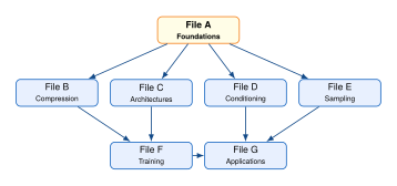
- Foundations (you are here)
Why video is hard, the spatiotemporal data manifold, the three-pillar framework, extending image diffusion to video, and the computational challenge.
- Compression
sec:vdiff:video-ae,sec:vdiff:causal-3dvae, sec:vdiff:discrete-tokens,sec:vdiff:latent-temporal: video autoencoders and the metrics that judge them; causal 3D VAEs, from 3D convolutions and the left-padding trick to the full training objective; discrete tokenisation by vector quantisation and lookup-free quantisation; and the temporal structure of the resulting latent space.
- Architectures
sec:vdiff:dit,sec:vdiff:factored-attn, sec:vdiff:3d-pe,sec:vdiff:conditioning,sec:vdiff:moe: spatiotemporal patchification and the video Diffusion Transformer with adaLN-Zero; the central efficiency decision of factoring attention; 3D RoPE and length generalisation; the three conditioning pathways; and mixture-of-experts layers.
- Objectives, sampling and training
sec:vdiff:noise-schedules,sec:vdiff:flow-matching, sec:vdiff:sampling-acceleration,sec:vdiff:training-scale: why image noise schedules must be shifted for video; flow matching on optimal-transport paths and rectified flow; sampling acceleration by distillation and feature caching; and multi-stage training at scale, including data curation and resolution curricula.
- Control and personalisation
sec:vdiff:cfg-video,sec:vdiff:i2v, sec:vdiff:motion-camera,sec:vdiff:t2v-pipeline, sec:vdiff:personalisation: multi-condition classifier-free guidance; image-to-video; camera control via Plücker rays and video ControlNets; LLM prompt enhancement and the full text-to-video pipeline; and LoRA and DreamBooth personalisation.
- Long video and world models
sec:vdiff:long-video,sec:vdiff:temporal-consistency, sec:vdiff:editing,sec:vdiff:physics,sec:vdiff:ar-diffusion: autoregressive chunking and hierarchical keyframes for long-horizon generation; measuring and enforcing temporal consistency; video editing; physics-aware generation and the “is this a world model?” question; and autoregressive-diffusion hybrids.
- Evaluation, applications and synthesis
sec:vdiff:evaluation,sec:vdiff:applications, sec:vdiff:connections,sec:vdiff:open-problems: FVD and decomposed benchmarks such as VBench; specialised applications from human motion to talking heads; connections to the rest of the book; and five open problems.
Key Idea.
The central question of this chapter. How do we extend the diffusion framework from the image domain to the video domain in a way that is computationally tractable, temporally coherent, and controllable? Every technique in this chapter addresses some facet of this question.
The Spatiotemporal Data Manifold
Before we can build models that generate video, we must understand the mathematical structure of the data they aim to produce. In this section, we formalise video as a mathematical object, introduce the key structural properties that distinguish video from collections of independent images, and develop the notation that will serve us throughout the chapter.
Video as a continuous function
At the most abstract level, a video is a function that maps spacetime coordinates to colour values. Let denote the video duration in seconds. We define:
Definition 1 (Continuous video signal).
A continuous video signal is a function (Continuous Video) where the first argument is time , the spatial arguments are normalised image coordinates, and the output is a -dimensional colour vector (e.g., for RGB).
In practice, we never observe in its continuous form. Cameras sample this function on a discrete grid determined by the frame rate (temporal sampling) and the sensor resolution (spatial sampling). This gives rise to the video tensor.
Definition 2 (Video tensor).
Given a continuous video signal , the video tensor is defined by sampling on a regular grid: (Video Tensor) where is the frame rate (frames per second), is the number of frames (so a 5-second clip at 24 fps has frames, sampled at times ), and are the spatial height and width in pixels, and is the number of colour channels.
Remark 2 (Notation conventions).
Throughout this chapter, we use the following conventions:
denote 4D video tensors (bold calligraphic, following the
tXnotation).denotes the -th frame of a video, obtained by slicing: .
denotes a single image (a vectorised frame) when context is clear.
Superscripts index frames (); subscripts index diffusion time (). Thus is frame at diffusion timestep .
The Nyquist perspective
The continuous-to-discrete transition is governed by the Nyquist-Shannon sampling theorem. Temporally, a video sampled at fps can faithfully represent motion frequencies up to Hz. A spinning wheel at 13 Hz sampled at 24 fps will alias, appearing to rotate backwards (the wagon-wheel effect). Spatially, the sensor resolution limits the spatial frequencies that can be captured.
Proposition 1 (Temporal Nyquist bound).
Let be a continuous video signal whose temporal spectrum (at each spatial location) is band-limited to Hz. Then can be perfectly reconstructed from its temporal samples whenever the frame rate satisfies . Conversely, if there exist distinct band-limited signals with identical samples, so no reconstruction rule can recover in general.
Proof.
This is a direct application of the classical Shannon sampling theorem to the temporal axis. For each fixed spatial location , the function is a band-limited signal, and the standard reconstruction formula (SINC Reconstruction) recovers whenever . (The boundary case also suffices provided the spectrum carries no atom at ; a pure sinusoid at exactly Hz sampled at fps is the standard counterexample.) For the converse, if then two sinusoids at frequencies and , both inside , produce identical samples.
This proposition has a practical implication for video generation: the frame rate of the generated video determines the highest temporal frequency that can be represented. A model generating at 8 fps cannot faithfully represent fast motions that require 24 fps to resolve; it can only produce temporally smooth, low-frequency motion.
Optical flow and the brightness constancy equation
One of the most important structural properties of natural video is the relationship between adjacent frames induced by object motion. If a scene point moves with velocity in the image plane, and its brightness does not change during the motion, then the brightness constancy equation holds:
(Brightness Constancy) where is the image intensity at time and spatial location , and is the spatial gradient.
Definition 3 (Optical flow field).
The optical flow field between frames and is a vector field (FLOW Field) that assigns to each pixel in frame its displacement such that the corresponding point in frame is located at .
Remark 3 (Flow as a soft constraint for generation).
While the brightness constancy equation is an idealisation (it ignores occlusions, lighting changes, and non-Lambertian surfaces), it captures a strong statistical regularity of natural video. Video generation models implicitly learn to respect this constraint: frames generated by a well-trained model will exhibit smooth, physically plausible optical flow fields, even though the model is never explicitly trained on flow. A separate family of methods goes further and conditions the denoiser on an explicitly supplied flow or trajectory field, using it as an intermediate representation that the user can edit directly; we return to these in Motion and Camera Control.
Insight.
Optical flow reveals the low-dimensional structure of video. Despite the enormous dimensionality of the video tensor, the set of “natural” videos lies on a much lower-dimensional manifold. Optical flow is one manifestation of this: instead of specifying all values of the next frame independently, it suffices to specify a -dimensional displacement at each pixel (plus a residual for dis-occluded regions). This reduces the effective per-frame dimensionality from to roughly , where accounts for new content. The compression methods of Video Autoencoders exploit this structure directly.
Temporal autocorrelation
The statistical relationship between frames at different time offsets is captured by the temporal autocorrelation function.
Definition 4 (Temporal autocorrelation).
Let denote the vectorised -th frame of a video drawn from the data distribution . The temporal autocorrelation matrix at lag is (Autocorrelation) where the expectation is over videos sampled from the data distribution and over frame indices . When the video is (wide-sense) stationary, depends only on the lag , not on the absolute frame index .
For natural video, the autocorrelation decays smoothly with lag, reflecting the fact that nearby frames are highly similar while distant frames may depict entirely different content. This decay rate varies dramatically across video types: a static surveillance camera produces near-constant autocorrelation, while an action movie has rapid decay due to frequent cuts and fast motion.
Proposition 2 (Exponential autocorrelation decay).
For a class of natural videos with stationary statistics and smooth motion, the normalised autocorrelation is well-approximated by an exponential decay: (EXP Decay) where is a characteristic decorrelation timescale measured in frames.
Sketch of proof.
Model each pixel trajectory as an Ornstein-Uhlenbeck process , whose autocorrelation is exactly . Summing over all pixel trajectories and normalising gives the desired form with . While individual pixel trajectories are not exactly Ornstein-Uhlenbeck, the averaged autocorrelation across all pixels and videos in a dataset empirically follows this exponential form.
The decorrelation timescale has direct implications for model design. A model with a temporal receptive field of frames can capture correlations up to lag ; if , the model will miss long-range temporal dependencies and produce temporally incoherent output.
Example 2 (Decorrelation timescales for different video types).
Typical decorrelation timescales (at 24 fps) for different video categories:
Surveillance footage: frames (8–20 seconds). Nearly static backgrounds with slow foreground motion.
Talking head: frames (2–4 seconds). The background is static; facial movements provide moderate temporal variation.
Action/sports: frames (0.4–1.2 seconds). Fast motion and frequent scene changes cause rapid decorrelation.
Music video with cuts: frames (0.2–0.6 seconds). Scene cuts create near-instantaneous decorrelation.
Formalising temporal coherence
We now give a formal definition of temporal coherence, the most important structural property that distinguishes video from a random sequence of images.
Definition 5 (Temporal coherence).
Let be a video tensor with frames . We say that is -temporally coherent with respect to a distance function if (Temporal Coherence) where is a coherence threshold. Common choices for include:
distance: ;
Perceptual distance: for a learned feature extractor ;
Flow-warped distance: , where is the warping operator using optical flow .
Remark 4 (Coherence vs. quality).
Temporal coherence and per-frame quality are distinct (and sometimes competing) objectives. A model that copies the first frame identically to all subsequent frames achieves perfect temporal coherence () but zero dynamism. Conversely, a model that independently generates each frame from the same text prompt may produce individually beautiful frames that, when played as video, exhibit jarring flicker and identity changes. The art of video generation lies in balancing these two desiderata.
Lemma 1 (Coherence implies bounded total variation).
If a video is -temporally coherent, then its temporal total variation is bounded: (Temporal TV) Moreover, by the triangle inequality, the distance between any two frames satisfies: (Frame Distance Bound)
Proof.
Both bounds follow directly from the definition of temporal coherence and the triangle inequality for the metric . The total variation bound sums terms, each bounded by . The frame distance bound sums only terms.
This lemma reveals an important property: temporal coherence constrains how much a video can change over any time interval. A tightly coherent video (small ) can only depict slow changes; depicting fast motion requires either larger or a higher frame rate (so that each individual frame-to-frame change is small even though the overall motion is fast).
Exercise 2 (Coherence under subsampling).
Suppose a video with frames is -temporally coherent. Consider the temporally subsampled video obtained by keeping every -th frame.
Show that is -temporally coherent.
Under what conditions on and does the subsampled video remain perceptually smooth? Relate your answer to the Nyquist bound from Proposition 1.
Argue that this result justifies temporal compression in video autoencoders: if the original video is highly coherent (small ), we can subsample aggressively without losing temporal smoothness.
The video manifold hypothesis
The manifold hypothesis, well-established in the image domain, posits that high-dimensional data concentrates near a much lower-dimensional manifold. For video, this hypothesis is even more compelling: the constraints of physics, scene composition, and visual coherence restrict the set of plausible videos to a tiny fraction of the ambient space .
Proposition 3 (Intrinsic dimensionality of video).
Let be the manifold of natural videos. Its intrinsic dimensionality can be decomposed as: (Intrinsic DIM) where captures the degrees of freedom of the scene layout, captures per-frame local deformations (typically proportional to the number of moving objects), captures texture and lighting parameters, and captures the camera trajectory (at most for a freely moving camera, but typically much less due to smoothness constraints).
Remark 5 (Compression targets the manifold).
The intrinsic dimensionality estimate explains why video compression works so well: a 5-second, 720p video has ambient dimensionality , but its intrinsic dimensionality might be only to . The goal of a video autoencoder (Video Autoencoders) is to find a latent representation whose dimensionality is close to , achieving maximum compression with minimal information loss.
Visualising the spatiotemporal structure
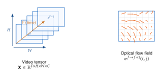
Exercise 3 (Frame interpolation and flow).
Let and be two consecutive frames with optical flow , and assume for simplicity that is constant over the interval. A point sitting at in the interpolated frame at fractional time (for ) came from in frame and travels on to in frame . Blending the two sources gives (Interpolation)
Show that and exactly. Show further that when brightness constancy holds exactly, the two sampled values agree, , for every - so the blending weights are irrelevant and the interpolant is exact. (Contrast this with the naive blend , which ghosts whenever .)
Explain why this linear model fails at occlusion boundaries (where one object moves in front of another).
Propose a modification using a learned occlusion mask that could handle occlusions more gracefully.
Three Pillars of Video Generation
Every successful video generation system, regardless of its specific architecture, must address three fundamental challenges. We call these the three pillars of video generation: compression, dynamics, and control. This taxonomy provides a unifying lens through which to understand the diverse landscape of methods we will encounter throughout the chapter.
Definition 6 (Video generation pipeline).
A video generation pipeline is built from three components , where:
is an encoder that compresses the video into a lower-dimensional latent representation ();
is a sampler (generative model) that produces samples from a learned distribution over the latent space, potentially conditioned on external signals;
is a decoder that maps the latent sample back to pixel space.
The encoder and the decoder play asymmetric roles. At training time the encoder defines the space the sampler learns in, ; at generation time it is not used at all, and the pipeline is the two-fold composition (Generation) where is a latent video tensor produced by the sampler for conditioning signal . (The encoder reappears at generation time only for conditional tasks such as image-to-video or editing, where an observed frame or clip must first be mapped into the latent space.)
Remark 6 (Pixel-space vs. latent-space generation).
Some early methods (e.g., VDM [3]) operate directly in pixel space, setting . This simplifies the pipeline but incurs enormous computational cost. Modern methods almost universally operate in a compressed latent space, with the encoder/decoder pair trained separately (or jointly) as a video autoencoder. We cover this compression stage in detail in sec:vdiff:video-ae,sec:vdiff:causal-3dvae.
Pillar 1: Compression
The first pillar addresses the dimensionality challenge: how to reduce the video tensor to a manageable size without losing information critical for reconstruction. The key insight is that natural videos have enormous redundancy, both spatial (neighbouring pixels are correlated) and temporal (adjacent frames share most of their content).
Spatial compression.
A standard image VAE [12] compresses each frame independently, reducing spatial resolution by a factor of (typically ). This transforms to , achieving a compression ratio of per frame.
Temporal compression.
Adjacent frames share so much content that we can also compress along the time axis. A temporal compression factor of reduces frames to latent frames. Combined with spatial compression, the total compression ratio becomes (Compression Ratio VAE)
Example 3 (Compression ratios in practice).
Consider a video with , , , . Several compression configurations and their resulting latent sizes:
tableEffect of different compression factors on latent
dimensions and compression ratios.
Latent shape Latent size Ratio 1 8 8 4 4 8 8 4 4 8 8 16 4 16 16 4
The compression-quality tradeoff.
Higher compression ratios reduce the computational burden on the sampler but inevitably lose fine-grained details. The autoencoder's reconstruction quality sets an upper bound on the generated video quality: no matter how good the sampler is, it cannot produce details that the decoder cannot reconstruct. Finding the right compression ratio is a critical design decision.
Insight.
Asymmetric compression. Spatial and temporal compression have different effects on perceived quality. Aggressive spatial compression () causes blurriness and loss of texture detail. Aggressive temporal compression () causes jerky motion and temporal aliasing. In practice, systems tend to compress more aggressively spatially than temporally, because temporal artifacts are more perceptually salient than spatial ones at moderate viewing distances.
Pillar 2: Dynamics
The second pillar is the most distinctive aspect of video generation: modelling the temporal evolution of visual content. This is where video generation fundamentally departs from image generation. The sampler must produce latent tensors whose frames, when decoded, form a temporally coherent sequence.
Factored dynamics.
A common approach factorises the denoiser into interleaved spatial and temporal blocks. Writing the network as a composition of block pairs, (Factored Denoiser) where each processes every frame independently (inheriting its weights from an image diffusion model) and each mixes information across frames at a fixed spatial location. Note that the blocks are composed, not added: the two branches are not two competing noise predictions but two stages of one network. The temporal blocks are typically zero-initialised, so that at the start of training the video model reproduces the pretrained image model applied frame by frame. This factorisation enables transfer from pretrained image models and reduces the computational cost of temporal modelling.
Attention-based dynamics.
The dominant mechanism for modelling dynamics in modern video diffusion models is temporal attention: given a sequence of per-frame features , temporal attention computes (Temporal Attention) where are the query, key, and value projection matrices and is the head dimension.
Convolutional dynamics.
An alternative is to use 1D convolutions along the time axis (or 3D convolutions jointly over space and time). These capture local temporal patterns efficiently but have limited receptive fields. In practice, many architectures combine temporal convolutions for local patterns with temporal attention for global coherence.
Definition 7 (Temporal receptive field).
The temporal receptive field of a video generation model at frame is the set of frames that can influence the model's prediction at frame through the network's connectivity. For a model with layers of temporal attention, (global receptive field). For a model with layers of temporal convolutions with kernel size , the receptive field has size .
Remark 7 (The dynamics spectrum).
Different video categories require dynamics modelling at different scales:
Sub-frame: motion blur, interlacing artifacts (requires understanding of exposure time).
Frame-to-frame: object motion, camera movement, lighting changes (the primary target of temporal attention).
Shot-level: character actions, physical interactions, narrative beats (requires multi-second temporal context).
Scene-level: establishing shots, transitions, cuts (requires understanding of cinematic language).
No single mechanism handles all of these well, which is why modern systems often use hierarchical temporal modelling with different mechanisms at different scales.
Pillar 3: Control
The third pillar addresses how to steer the generation process toward desired outputs. Without control, a video generation model is a random video sampler, interesting theoretically but of limited practical utility. Control comes in many forms.
Text conditioning.
The most common control signal is a text prompt, injected via cross-attention between the text embedding and the diffusion model's internal representations. Let be the sequence of text token embeddings from a frozen language model. (We reserve for the number of network layers throughout the chapter, so the prompt length gets its own symbol.) Cross-attention computes: (Cross Attention) where is the spatial-temporal feature at a given position and the softmax operates over the text sequence length .
Image conditioning.
Image-to-video generation conditions on one or more reference frames. The conditioning image can be injected by concatenation (appending it as an extra channel to the noisy input), by cross-attention, or by replacing the first frame of the noisy sequence with the (possibly encoded) conditioning image.
Structural control.
Fine-grained control over motion and layout can be achieved through auxiliary conditioning signals: depth maps, pose sequences, edge maps, segmentation masks, or motion trajectories. These are typically injected through lightweight adapter networks (ControlNets [61]) that leave the base model unchanged.
Example 4 (Control signal taxonomy).
tab:vdiff:control-signals classifies common control signals by their dimensionality and the type of guidance they provide.
tableTaxonomy of control signals for video generation.
Signal Shape Guidance type Injection method Text prompt Semantic Cross-attention Reference image Appearance Concat / cross-attn Depth sequence Geometric ControlNet Pose sequence Skeletal ControlNet Optical flow Motion ControlNet / warp Audio waveform Temporal rhythm Cross-attention Camera trajectory Viewpoint FiLM / concat
Classifier-free guidance for video.
As in image diffusion, classifier-free guidance (CFG) [62] amplifies the influence of the conditioning signal by extrapolating away from the unconditional prediction: (CFG) where is the guidance scale and denotes the null conditioning. We use this convention throughout the chapter: recovers the ordinary conditional prediction and extrapolates beyond it. (The literature also writes CFG as ; the two scales differ by one, , so quoted numerical ranges must always be read together with their convention.) For video, CFG can be applied jointly to all frames (preserving temporal coherence in the guidance direction) or independently per frame (risking temporal artifacts).
Caution.
Over-guidance causes temporal artifacts. While increasing the guidance scale in (CFG) improves text-video alignment and per-frame quality, excessively large amplifies high-frequency spatial details at the expense of temporal smoothness. This creates a flickering effect where fine textures “pop” in and out between frames. In practice, video models use lower guidance scales () than image models () to maintain temporal stability.
The three-pillar framework: a unified view
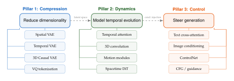
Figure 4 shows how different techniques map onto the three-pillar framework. Every video generation system makes specific design choices for each pillar, and the interplay between these choices determines the system's capabilities and limitations. For instance, Sora [6] uses a spacetime patchifier for compression (Pillar 1), a Diffusion Transformer for dynamics (Pillar 2), and text cross-attention with classifier-free guidance for control (Pillar 3).
Exercise 4 (Mapping methods to pillars).
Example 5 (Sora as a three-pillar system).
OpenAI's Sora [6] provides an instructive case study for the three-pillar framework:
Pillar 1 (Compression): Sora uses a spacetime patchifier that divides the video into non-overlapping patches (e.g., ), projects each patch into a -dimensional token, and processes the resulting sequence. This achieves a compression ratio of per patch. Crucially, the same patchifier handles different resolutions and aspect ratios by simply producing different numbers of tokens.
Pillar 2 (Dynamics): The dynamics model is a Diffusion Transformer (DiT) [9] that applies full self-attention over all spacetime tokens. By not factorising attention into spatial and temporal components, Sora allows every patch to attend to every other patch across space and time, enabling the model to learn long-range spatiotemporal dependencies. The computational cost is managed by (a) using a relatively large patch size (few tokens) and (b) employing massive compute budgets during training and inference.
Pillar 3 (Control): Text conditioning is injected via cross-attention layers interleaved with the self-attention layers. The text encoder is a large pretrained language model. Classifier-free guidance steers the generation toward the prompt.
Remark 8 (The pillar interaction principle).
The three pillars are not independent design choices; they interact strongly. A more aggressive compression (Pillar 1) reduces the token count, enabling more expressive dynamics models (Pillar 2) at the same computational budget. Richer control signals (Pillar 3) may require larger models (Pillar 2) to process effectively. Conversely, a weaker encoder (Pillar 1) that discards fine details shifts the burden to the decoder and limits the control precision achievable in Pillar 3. The best systems co-design all three pillars jointly.
From Image Diffusion to Video Diffusion
In this section, we make the conceptual leap from image diffusion to video diffusion precise. We show that the mathematical framework of diffusion models extends naturally to video tensors, but that the resulting model must satisfy structural requirements that go far beyond anything needed for images. We assume familiarity with the image diffusion framework from 19, particularly the DDPM training objective and the reparameterisation trick.
The joint forward process
Recall that in image diffusion, the forward process gradually corrupts a clean image by adding Gaussian noise according to a variance schedule : (Image Forward) where and . For video, we simply replace the image with the video tensor , treating the entire video as a single high-dimensional object.
Theorem 1 (Video forward process).
Let be a clean video tensor (in latent space). The forward process with noise schedule is: (Video Forward) where is the identity matrix of dimension , and . Equivalently, using the reparameterisation trick: (Video Reparam) The noise has the same shape as , with each element drawn independently.
Proof.
The forward process treats as a vector in and applies the standard Gaussian diffusion kernel. The Markov chain telescopes exactly as in the image case (see 19), giving The derivation is identical because the forward process operates element-wise and does not depend on the tensor's spatial or temporal structure.
Remark 9 (The noise is structureless).
A crucial observation: in (Video Reparam), the noise is drawn i.i.d. across all spatial locations and all frames. This means the forward process destroys temporal correlations at the same rate as spatial correlations. At (full noise), the noisy tensor is pure isotropic Gaussian noise with no spatial or temporal structure whatsoever. All the burden of creating spatiotemporal structure falls on the reverse process.
Example 6 (Signal-to-noise ratio across diffusion time).
The signal-to-noise ratio (SNR) at diffusion time is defined as (SNR) For a cosine noise schedule with , representative values are:
| 0 | 100 | 250 | 500 | 750 | 1000 | |
| 1.000 | 0.975 | 0.854 | 0.500 | 0.146 | 0.000 | |
| 39.0 | 5.85 | 1.00 | 0.171 | 0.000 |
Corollary 1 (Temporal SNR is uniform).
Since the forward process applies the same noise level to all frames, the per-frame SNR is identical across all frames at any given diffusion time . Formally, for any frames and : (PER Frame SNR) where the approximation uses the law of large numbers ( and for standardised data). This uniformity is a design choice, not a necessity; one could imagine noise schedules that add more noise to certain frames (e.g., middle frames) than others (e.g., boundary frames used for conditioning).
Why independent frame diffusion fails
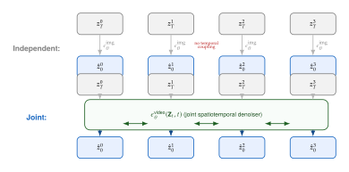
The simplest approach to video diffusion would be to apply an image diffusion model independently to each frame. This is tempting because it allows direct reuse of powerful pretrained image models. However, it fails catastrophically.
Remark 10 (Why independent frame diffusion fails).
Let be a video consisting of frames. The true data distribution is a joint distribution over all frames. Independent frame diffusion models the factorised distribution (Independent Factorisation) This factorisation ignores all inter-frame dependencies. Each frame is sampled from the correct marginal (assuming the image model is well-trained), but there is no mechanism to enforce consistency across frames.
The consequences are immediate and severe:
Identity drift: a person's face changes appearance from frame to frame.
Temporal flicker: high-frequency random variations in colour, texture, and lighting.
Incoherent motion: objects appear and disappear randomly instead of moving smoothly.
Violated physics: gravity, momentum, and object permanence are not preserved.
Insight.
The gap between marginals and joints. The failure of independent frame diffusion illustrates a deep statistical principle: matching marginal distributions does not imply matching the joint distribution. Formally, a collection of marginals pins the joint down only up to its copula: by Sklar's theorem, every joint consistent with those marginals is obtained by coupling them with some copula, and unless the marginals are degenerate (point masses) there are uncountably many copulas to choose from. The Fréchet-Hoeffding inequalities bound that family but do not select a member of it. The product distribution is just one such joint, and for natural video, it is a particularly poor one. The copula (the dependence structure independent of marginals) is what distinguishes video from a slideshow, and it is precisely what the temporal components of a video diffusion model must learn.
Example 7 (Independent vs. joint generation).
Consider generating a 3-frame video of a ball bouncing. Let denote the ball's position in frame . Under the true distribution: (BALL Trajectory) where is gravitational acceleration. The positions are deterministically coupled given the initial conditions. Under the independent model, each is sampled independently from the marginal over ball positions, producing a ball that teleports randomly around the scene.
Exercise 5 (KL divergence between joint and product).
Let be the true joint distribution of video frames, and let be the product of marginals.
Show that the KL divergence between the joint and the product decomposes as: (KL Joint Product) where is the mutual information between frame and all preceding frames.
Argue that for natural video, this quantity is enormous (on the order of thousands of nats per frame), explaining why the product approximation fails so badly.
What does this imply about the “information content” that temporal modelling must capture?
Remark 11 (Partially factorised approaches).
Between fully independent generation and fully joint generation lie several intermediate approaches:
Autoregressive: generate frames sequentially, conditioning each on all previous frames: . This captures all dependencies but prevents parallel generation across frames.
Markov: condition each frame only on the immediately preceding frame: . This reduces the conditioning context but loses long-range dependencies.
Block-joint: generate non-overlapping blocks of frames jointly, then stitch blocks together: . This balances joint modelling within blocks with autoregressive extension across blocks.
Modern systems typically use the block-joint approach, generating 16–32 frames jointly and extending to longer videos autoregressively.
The video DDPM training algorithm
The training procedure for video diffusion is a direct extension of image DDPM. The key change is that the denoiser now takes a video tensor as input and must predict noise for all frames jointly.
Algorithm 1 (Video DDPM training).
Input: Training video dataset , noise schedule , video encoder (pretrained and frozen). Output: Trained denoiser .
repeat
Sample a training video .
Encode: .
Sample diffusion timestep .
Sample noise , .
Construct noisy input: .
(Optional) Sample conditioning signal (e.g., text prompt) associated with .
Compute loss: .
Update via gradient descent on .
until convergence.
Remark 12 (Training vs. image DDPM: what changes?).
Algorithmically, the training loop in Algorithm 1 is nearly identical to image DDPM. The differences lie entirely in the architecture of :
The input and output have an additional temporal dimension .
The network must include temporal modelling components (temporal attention, temporal convolutions) in addition to the standard spatial components.
The conditioning signal may include temporal information (e.g., per-frame text descriptions, audio features, or pose sequences).
The noise schedule , the loss function, and the optimisation procedure are identical. This mathematical simplicity is one of the great strengths of the diffusion framework: the same training objective works for images, video, 3D shapes, audio, and any other continuous data modality.
The denoiser must learn spatiotemporal structure
We now state a key proposition that motivates the architectural innovations of sec:vdiff:dit,sec:vdiff:factored-attn.
Proposition 4 (Spatiotemporal denoiser requirement).
Let be the denoiser in a video diffusion model trained with the objective in Algorithm 1. At optimality, (Optimal Denoiser) where is the posterior mean of the clean video given the noisy observation. This posterior mean is not decomposable across frames: (NON Decomposable)
Proof.
The first statement follows from the standard result that the MSE-optimal predictor of given is the conditional expectation , combined with the reparameterisation . Solving that identity for gives ; taking conditional expectations of both sides and using linearity yields (Optimal Denoiser).
For the non-decomposability, observe that (Posterior MEAN Integral) The posterior factorises as (Posterior Bayes) While factorises across elements (since the noise is i.i.d.), the prior does not factorise across frames (since natural videos have strong inter-frame dependencies). Therefore does not factorise, and its mean is not decomposable.
Insight.
The information-theoretic view. Consider the mutual information between clean frame and noisy frame at diffusion time . When , this quantity is zero in the forward process (noise is independent), but positive in the posterior (because knowing provides information about via the prior, which in turn provides information about ). The denoiser must exploit this indirect information pathway: noisy frame at time tells us something about clean frame through the prior's temporal correlations. This is why the denoiser must attend to all frames jointly.
The reverse process and sampling
The reverse process mirrors the image case. Starting from , we iteratively denoise: (Reverse) where the predicted mean is (Predicted MEAN)
Algorithm 2 (Video DDPM sampling).
Input: Trained denoiser , noise schedule , video decoder , conditioning signal . Output: Generated video .
Sample , .
for do
Sample if , else .
.
end for
Decode: .
return .
Remark 13 (Sampling cost).
Each step of the reverse process requires a full forward pass through the denoiser , which processes the entire video tensor . With diffusion steps (or 50 steps with DDIM [10]), the total sampling cost is times the cost of a single denoiser evaluation. For video, each evaluation is itself extremely expensive (as we quantify in The Computational Challenge), making efficient sampling critical.
Exercise 6 (Interpolation in diffusion space).
Let and be two clean video latents. Consider the spherical linear interpolation (slerp) of their noised versions at diffusion time : (Slerp Interp) where .
Show that when (i.e., slerp preserves norm).
If both and depict the same scene with different camera angles, describe qualitatively what you expect to see when denoising .
Why is slerp preferred over linear interpolation in high-dimensional spaces?
Exercise 7 (Video ELBO derivation).
Derive the ELBO for video diffusion by treating as a high-dimensional vector and applying the standard VDM ELBO derivation from 19. Show that the resulting objective decomposes as: (Video ELBO) Verify that the simplified training objective is a reweighted version of the denoising matching terms.
The Computational Challenge
We have established that video diffusion is mathematically straightforward: simply apply the image diffusion framework to a higher-dimensional tensor. The devil, however, is in the computational details. In this section, we quantify the computational cost of naive video diffusion and show that it is prohibitively expensive, motivating the compression and architectural innovations discussed in the subsequent files.
The attention bottleneck
The dominant computational cost in modern diffusion models comes from self-attention layers. In an image diffusion model operating on a spatial grid of latent pixels, each self-attention layer has complexity: (Image Attention Flops) where is the attention head dimension. For video, if we apply full spatiotemporal attention (every position attends to every other position across all frames), the cost becomes: (Video Attention Flops)
Proposition 5 (Quadratic bottleneck).
The ratio of full spatiotemporal attention cost to per-frame spatial attention cost is: (Flops Ratio) That is, full spatiotemporal attention is times more expensive than applying spatial attention independently to each of the latent frames. Moreover, the absolute cost grows quadratically with the number of frames.
Proof.
Full spatiotemporal attention over tokens costs FLOPs. Independent spatial attention over frames, each with tokens, costs . The ratio is:
Example 8 (Concrete compute estimates).
Let us compute the attention cost for a realistic video diffusion scenario. Consider generating a 5-second, 720p video at 24 fps with a latent-space model using spatial compression and temporal compression :
Pixel-space video:
Latent video: , , ,
Total latent tokens:
Attention head dimension: , with 16 heads
For a single attention layer: (FULL ATTN COST) The ratio is indeed : full spatiotemporal attention is 30 times more expensive than per-frame spatial attention.
With attention layers (typical for a DiT-XL model) and sampling steps (DDIM), the total attention cost for sampling one video is: (Total Sampling COST) An NVIDIA H100 has a peak BF16 tensor-core throughput of roughly 1 PFLOP/s, so even at peak this would take some 530 seconds, nearly 9 minutes for a single 5-second video.
Two caveats make this a floor rather than an estimate. First, the convention used above counts only the product; including the product doubles every absolute figure to (all ratios, including the factor above, are unaffected). Second, sustained throughput on attention is well below peak. The realistic wall-clock figure is therefore several times 9 minutes; the point of the calculation is the order of magnitude, not the constant.
Memory constraints
Beyond FLOPs, memory is often the binding constraint. Attention requires storing the key-value (KV) matrices for all tokens: (KV Memory) where is the total number of tokens, is the number of attention heads, is the number of layers, and is the bytes per element (2 for FP16/BF16, 1 for FP8).
Example 9 (KV cache memory).
Continuing the previous example (, , , , BF16 precision): (KV Memory Concrete) The KV cache alone therefore occupies well over half of a single H100's 80 GB of HBM3, before a single parameter or activation has been stored. Adding the model parameters (2–8 GB), the activations retained for backpropagation (3–5 the KV cache, i.e. 150–250 GB), and the video tensor itself takes the total well past 200 GB, so training at this token count requires model parallelism across several GPUs even for modest video lengths.
Caution.
Memory, not FLOPs, is the true bottleneck. In many practical settings, the memory required to store attention matrices and KV caches exceeds GPU memory long before the FLOPs become prohibitive. This is because memory scales as per layer (for the KV cache) plus for the attention matrix itself (unless using memory-efficient attention implementations like FlashAttention [11]). With FlashAttention, the attention matrix is never materialised, but the KV cache remains.
Scaling analysis
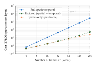
Figure 6 illustrates how different attention strategies scale with the number of latent frames. The quadratic cost of full spatiotemporal attention becomes prohibitive beyond latent frames: at the temporal compression and 24 fps of Example 8 that is roughly five seconds of video, and a single attention layer already costs over 400 TFLOPs. This motivates two complementary strategies, taken up in turn in the two stages that follow:
Compress more aggressively (Video Autoencoders): reduce , , and through better video autoencoders, directly reducing the token count .
Factorise attention (Factored Attention for Video): replace full spatiotemporal attention with separate spatial and temporal attention passes, reducing the cost from to .
Proposition 6 (Factored attention savings).
Let the cost of full spatiotemporal attention be . Factored attention (spatial attention within each frame, followed by temporal attention at each spatial location) costs (Factored COST) The savings ratio is: (Savings Ratio) where the approximation holds when (typical case) or (rare). For and , the savings ratio is approximately .
Proof.
Direct computation. When , the spatial term dominates , so When , the temporal term dominates:
Scaling with resolution and duration
The computational cost of video generation scales polynomially with all three axes: spatial resolution, temporal duration, and model size. Let us write the total cost of sampling a video as: (Total COST) where is the number of diffusion sampling steps, is the number of transformer layers, is the per-layer attention cost, and accounts for feedforward layers, normalisations, and the decoder.
| Parameter doubled | Cost multiplier (full attn) | Cost multiplier (factored) |
| Side length ( and ) | ||
| Duration () | ||
| Model depth () | ||
| Head dimension () | ||
| Sampling steps () |
Remark 14 (The cost of high quality).
Table 1 reveals why high-resolution, long-duration video generation remains so challenging. Going from a , 2-second preview to a , 16-second production video multiplies each side length by (so the token count per frame grows by ) and the frame count by ; the total token count therefore grows by . Because attention is quadratic, not linear, in the token count, the cost grows far faster than that:
Full attention, , grows by ;
Factored attention, , grows by in its spatial term and in its temporal term; since the spatial term dominates, the total grows by roughly .
Even the factored architecture, in other words, pays more than three orders of magnitude for the jump from preview to production quality, and full attention pays more than four. Note how much larger these numbers are than the naive “” one gets by treating cost as linear in : the quadratic term is the whole story. This explains why current commercial systems often generate short, low-resolution previews first and then upsample using super-resolution cascades or tile-based approaches.
The memory wall
Even with FlashAttention eliminating the memory cost of the attention matrix, video diffusion models face a “memory wall” from three sources:
Model parameters: A DiT-XL model has 675M parameters (1.35 GB in FP16). Scaled-up video models can exceed 10B parameters (20 GB in FP16).
Activations: During training, intermediate activations must be stored for backpropagation. With layers, tokens, and BF16 storage, a single tensor costs 0.88 GB per layer, so the two tensors per layer counted by already come to 50 GB. A real DiT block retains many more than two - the QKV projections, the attention output, and above all the -wide MLP hidden state, which alone costs four times a single -wide tensor - so the true figure comfortably exceeds 200 GB.
The video tensor itself: The full-resolution input/output video must fit in memory during encoding and decoding. A single 720p, 120-frame video in FP32 requires GB.
Insight.
The memory-compute tradeoff. Gradient checkpointing can reduce activation memory at the cost of recomputation. By storing activations at only every -th layer and recomputing the others during the backward pass, memory is reduced by a factor of . The price is one extra partial forward pass: for half the layers are recomputed, and since a training step costs roughly one forward plus two backward units, this adds about to the total. (Recomputing every layer, the limit, costs a full extra forward pass, or about 33%.) For video diffusion, aggressive gradient checkpointing (large ) is standard practice, trading compute (which can be parallelised across GPUs) for memory (which cannot).
Exercise 8 (Memory budget analysis).
You have access to a single NVIDIA A100 GPU with 80 GB of HBM2e memory. You want to train a video diffusion model with the following specifications:
Model: 24 transformer layers, hidden dimension 1024, 16 attention heads, 350M parameters.
Latent video: , , , .
Batch size: 1 (single video per GPU).
Precision: BF16 (2 bytes per parameter/activation).
Calculate the memory required for model parameters (including optimizer states for AdamW, which stores two additional copies of the parameters in FP32).
Calculate the memory required for the KV cache of the attention layers.
Calculate the peak activation memory without gradient checkpointing.
Determine whether the model fits in 80 GB. If not, what is the maximum that fits?
Comparison to other generative modalities
It is instructive to compare the computational demands of video generation to other generative modalities, as this comparison highlights why video remains the most challenging frontier.
Example 10 (Cross-modality compute comparison).
tab:vdiff:cross-modality compares the typical computational cost of generating samples across different modalities using state-of-the-art models (circa 2025).
tableApproximate computational cost of generating one sample
across different modalities. Costs are per-sample on an H100 GPU.
Modality Output size Tokens Time (s) Text (LLM, 1K tokens) 1K tokens 1,000 0.5–2 Image () 4,096 2–10 Audio (10 s, 44 kHz) 441K samples 10,000 5–20 Video (5 s, 720p) 400,000 60–600 3D scene (NeRF) Multi-view consistent varies 30–300
Remark 15 (The training cost gap).
The inference-time cost gap is dwarfed by the training-time gap. Training a state-of-the-art image diffusion model (e.g., Stable Diffusion XL) requires roughly 25,000 A100 GPU-hours. Training a comparable video model requires 10–100 more compute, primarily because: (a) each training sample (video) requires more FLOPs to process, (b) video datasets are less curated, requiring more epochs to learn, and (c) temporal consistency requires seeing diverse motion patterns, demanding larger and more diverse datasets. Sora's training cost has been estimated at over 1 million A100-equivalent GPU-hours.
Exercise 9 (Roofline analysis for video diffusion).
An NVIDIA H100 GPU has a peak throughput of 990 TFLOPS (BF16 tensor cores) and a memory bandwidth of 3.35 TB/s. The arithmetic intensity of an operation is defined as the ratio of FLOPs to bytes transferred.
Compute the arithmetic intensity of a matrix multiplication where and , with (video tokens) and . Is this operation compute-bound or memory-bound on the H100?
Compute the arithmetic intensity of the softmax operation for the same and . Is this compute-bound or memory-bound?
Using the roofline model, estimate the theoretical minimum time for a single full spatiotemporal attention layer with 16 heads.
How does FlashAttention change the roofline analysis? Hint: FlashAttention fuses the QK, softmax, and AV operations, reducing memory traffic at the cost of recomputation.
Summary and preview of solutions
The computational analysis in this section paints a clear picture: naive video diffusion, applying full spatiotemporal attention to all frames jointly, is prohibitively expensive for any video longer than a few seconds at modest resolution. Table 2 summarises the key challenges and the solutions we will develop in subsequent files.
| Challenge | Where addressed | Key technique |
| High-dimensional input | sec:vdiff:video-ae,sec:vdiff:causal-3dvae | Causal 3D video autoencoders with spatial and temporal compression |
| Quadratic attention cost | Factored Attention for Video | Factored spatial/temporal attention, 3D window attention |
| Conditioning complexity | sec:vdiff:conditioning,sec:vdiff:motion-camera | Cross-attention and adaLN pathways, ControlNet adapters |
| Slow sampling | Sampling Acceleration | Consistency distillation, feature caching, few-step solvers |
| Data and training scale | Training at Scale | Multi-stage resolution curricula, mixed image-video training, data curation |
| Drift over long horizons | Long Video Generation | Autoregressive chunking, hierarchical keyframes |
Key Idea.
The fundamental tradeoff. Video diffusion model design is governed by a three-way tradeoff between quality (per-frame fidelity and temporal coherence), efficiency (computational cost and memory usage), and controllability (the richness of conditioning signals the model can accept). Improving one dimension typically comes at the expense of another: higher quality requires more compute, richer control requires more parameters, and greater efficiency requires accepting some quality loss. The art of video diffusion model design lies in finding the sweet spot for the target application.
We now turn to the first and most impactful lever for reducing computational cost: compressing the video tensor into a compact latent representation. Video Autoencoders sets up video autoencoders and the reconstruction metrics that judge them; Causal 3D Variational Autoencoders builds the causal 3D VAE that has become the field's default, from 3D convolutions and the left-padding trick up to the full training objective; Discrete Tokenisation for Video covers the discrete alternative, vector quantisation and lookup-free quantisation; and Latent Space Temporal Structure closes the loop by showing that a temporally smooth video maps to a temporally smooth latent trajectory, which is precisely what makes latent video diffusion work at all.
Video Autoencoders
Diffusion models are powerful, but they are also expensive. The iterative denoising process that makes them work requires evaluating a neural network dozens or hundreds of times per sample, and each evaluation operates on a tensor whose size equals the output resolution. For images, this cost is manageable: a image contains roughly values. For video, the situation is dramatically worse. A modest -frame clip at resolution already contains million values; a -second clip at () and frames per second exceeds million values. Running a diffusion model directly in this pixel space is computationally prohibitive.
The solution, first demonstrated for images by Rombach et al. [14] in Latent Diffusion Models (LDMs), is to separate the problem into two stages. First, train an autoencoder that compresses the data into a compact latent space. Second, run the diffusion process in that latent space rather than in pixel space. The autoencoder absorbs the perceptual details (textures, edges, colour gradients) that do not require iterative refinement, while the diffusion model focuses on the semantic structure (object identity, motion, scene composition) that benefits from the iterative process.
For video, this two-stage strategy is not merely convenient; it is essential. The compression ratio determines the practical feasibility of the entire pipeline. In this section, we formalise the two principal approaches to video compression, spatial-only and spatiotemporal, and analyse the trade-offs that govern the design of video autoencoders.
Key Idea.
Compress first, then diffuse. The central engineering principle of latent video diffusion is to never run the denoising process in pixel space. Instead, an autoencoder maps the video to a latent tensor with . The diffusion model operates entirely on , and the decoder maps generated latents back to pixel space. This factorisation reduces computational cost by orders of magnitude while preserving perceptual quality.
Why Pixel-Space Video Diffusion Is Impractical
To appreciate the necessity of latent compression, let us quantify the computational burden of pixel-space video diffusion. Consider a video tensor . The diffusion model must process this tensor at every denoising step, and a typical generation requires steps (often to ).
Example 11 (Computational Cost of Pixel-Space Video Diffusion).
Consider generating a -second video at fps and resolution. The video tensor has shape , containing approximately million values. A U-Net processing this tensor at each of denoising steps must perform roughly billion element-wise operations per sample, before accounting for the quadratic cost of any attention layers.
By contrast, if an autoencoder compresses the video by a factor of (temporally spatially spatially), the latent tensor has shape , containing roughly values. The diffusion model now operates on a tensor that is smaller, reducing both memory and computation proportionally.
This example illustrates a broader principle: the autoencoder is not an optional optimisation but a structural prerequisite for video diffusion at practical resolutions.
Spatial-Only Compression
The simplest approach to video compression is to ignore the temporal dimension entirely and encode each frame independently using a pre-trained image autoencoder.
Definition 8 (Spatial-Only Video Autoencoder).
Let be a pre-trained image encoder and the corresponding decoder. The spatial-only video autoencoder applies these maps frame-by-frame: (Spatial ENC) where is the -th frame and is its latent code. The latent video tensor is the stack .
The spatial-only approach has clear advantages. It reuses image autoencoders (such as the one from Stable Diffusion) without any modification, inheriting their mature training and high reconstruction quality. The frame count is preserved in the latent space, so temporal modelling is left entirely to the diffusion model.
However, this design has a fundamental limitation: it completely ignores the temporal redundancy present in natural video. Consecutive frames in a video are highly correlated; objects move smoothly, lighting changes gradually, and backgrounds persist across many frames. A spatial-only encoder encodes each frame as if it were an independent image, wasting capacity on information that is redundant across time.
Remark 16.
The spatial-only approach preserves the frame count () but wastes temporal redundancy. The compression ratio is , which is independent of . For the Stable Diffusion VAE, this ratio is approximately ( spatial downsampling with channels). While this is substantial, the latent video remains large when is large because no temporal compression occurs.
Spatiotemporal Compression
To exploit temporal redundancy, we need an autoencoder that processes the video as a 3D volume rather than a stack of independent images.
Definition 9 (Spatiotemporal Video Autoencoder).
A spatiotemporal video autoencoder jointly encodes the entire video tensor: (3D ENC) where , , in general. The encoder and decoder use 3D convolutional or attention-based architectures that process spatial and temporal dimensions jointly.
The spatiotemporal approach compresses along all three dimensions simultaneously. Because consecutive frames share most of their content, the encoder can represent temporal redundancy far more efficiently than the spatial-only approach.
Definition 10 (Compression Ratio).
The compression ratio of a video autoencoder with input shape and latent shape is (Compression Ratio) A spatiotemporal autoencoder with temporal and spatial downsampling, mapping the input channels to latent channels, achieves , comparable to the spatial-only ratio but with the critical advantage that has also been reduced.
Comparing the Two Approaches
Table 3 summarises the key trade-offs between spatial-only and spatiotemporal video autoencoders.
| Property | Spatial-Only | Spatiotemporal |
| Temporal compression | None () | Yes () |
| Temporal redundancy | Not exploited | Exploited |
| Reuses image AE | Yes | No (new architecture) |
| Latent size for | ||
| Causal design needed | No | Yes (for streaming) |
| Training data | Images suffice | Videos required |
| Reconstruction quality | Per-frame optimal | Jointly optimised |
Remark 17.
The choice between spatial-only and spatiotemporal compression reflects a deeper architectural decision. Spatial-only compression delegates all temporal modelling to the diffusion model, which must then learn temporal coherence from scratch in the latent space. Spatiotemporal compression embeds temporal structure into the latent space itself, giving the diffusion model a head start. However, spatiotemporal compression introduces a new challenge: the encoder must be designed carefully to avoid “future leakage,” where the latent code for frame depends on frames . This motivates the causal architectures developed in Causal 3D Variational Autoencoders.
Architecture Overview
Figure 7 illustrates the two approaches side by side. The spatial-only encoder processes each frame through a 2D convolutional network, producing independent latent maps that are stacked along the time axis. The spatiotemporal encoder processes the entire video through a 3D convolutional network, producing a compressed latent volume with reduced temporal extent.
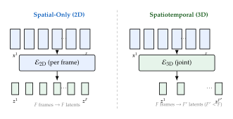
The connection between video autoencoders and the VAE theory developed in 15 is direct: both spatial-only and spatiotemporal video autoencoders are trained as variational autoencoders, optimising an ELBO that balances reconstruction fidelity against latent regularisation. The key differences lie in the architecture of the encoder and decoder (2D vs. 3D convolutions) and the structure of the latent space (independent per-frame vs. jointly compressed). The vector quantisation techniques from 16 also play a role, as we will see in Discrete Tokenisation for Video.
Insight.
The autoencoder is the unsung hero of video generation. While the diffusion model receives most of the attention in video generation papers, the quality of the autoencoder often determines the ceiling of the entire system. A poor autoencoder introduces artefacts (blurriness, colour shifts, flickering) that the diffusion model cannot correct, no matter how well it is trained. State-of-the-art video generation systems such as Sora, CogVideoX, and Wan-Video invest significant effort in training high-quality video autoencoders before turning to the diffusion component.
Reconstruction Quality Metrics
How do we measure the quality of a video autoencoder? Unlike text compression, where lossless reconstruction is the standard, video autoencoders are lossy by design. The quality of the lossy reconstruction must be measured along multiple axes.
Definition 11 (Video Reconstruction Metrics).
Let be the original video and the reconstruction. The following metrics are standard:
Peak Signal-to-Noise Ratio (PSNR): (PSNR) where is the maximum possible pixel value (typically for 8-bit video). Higher is better; values above dB indicate good reconstruction.
Structural Similarity Index (SSIM): Computed per-frame between and , averaging luminance, contrast, and structural comparisons over local windows. Values range from to ; values above indicate near-perceptual equivalence.
Learned Perceptual Image Patch Similarity (LPIPS): Computed as the distance between deep features extracted by a pre-trained network (VGG or AlexNet), summed over selected layers. Lower is better; this metric correlates well with human perceptual judgments.
Temporal consistency: Measured by the optical flow error between consecutive reconstructed frames. Given estimated flow fields from to , the warping error is .
Caution.
PSNR can be misleading for video autoencoders. A video autoencoder can achieve high PSNR by producing blurry reconstructions that average over fine details. This is because the mean squared error (which PSNR measures) penalises sharp but slightly misaligned details more heavily than uniform blur. For this reason, perceptual metrics (LPIPS) and temporal consistency metrics are essential complements to PSNR when evaluating video autoencoders.
Example 12 (Typical Reconstruction Quality).
For reference, state-of-the-art video autoencoders achieve the following approximate reconstruction metrics on standard benchmarks:
Spatial-only (Stable Diffusion VAE, spatial): PSNR – dB per frame, SSIM –, LPIPS –.
Spatiotemporal (CogVideoX, ): PSNR – dB, SSIM –, with improved temporal consistency scores compared to spatial-only.
Discrete (MAGVIT-v2, ): PSNR – dB, with lower per-frame quality but competitive FVD (Fréchet Video Distance) scores when combined with autoregressive priors.
Causal 3D Variational Autoencoders
The previous section motivated the need for spatiotemporal video compression and contrasted it with the simpler spatial-only approach. We now turn to the mathematical core of spatiotemporal video compression: the causal 3D variational autoencoder (Causal 3D-VAE). This architecture combines three ingredients: (1) 3D convolutions that process spatial and temporal dimensions jointly, (2) a causal masking scheme that prevents future frames from influencing past latents, and (3) a variational training objective that regularises the latent space for downstream diffusion.
The causality constraint is not merely a technical nicety. Without it, the latent code for frame would depend on all frames in the video, including frames . This creates two problems. First, it prevents autoregressive generation, where frames are produced sequentially and future frames are not yet available when encoding past frames. Second, it couples the latent representations in a way that makes it difficult for the diffusion model to generate temporally coherent video, because changing one frame's latent code would implicitly alter all other latent codes.
Historical Note.
From image VAEs to causal video VAEs. The journey from image to video autoencoders mirrors the broader evolution of generative modelling. Image autoencoders (Kingma & Welling, 2013 [12]; Van Oord et al., 2017 [13]) established the VAE and VQ-VAE frameworks. The Stable Diffusion VAE (Rombach et al., 2022 [14]) demonstrated that 2D autoencoders could serve as the compression backbone for latent diffusion. MAGVIT [15] and MAGVIT-v2 [16] introduced 3D tokenisers for video, using causal convolutions to support variable-length generation. CogVideoX [17] and Open-Sora [18] brought causal 3D-VAEs to the forefront of video diffusion, achieving state-of-the-art compression ratios. Most recently, Wan-Video [7] demonstrated a causal 3D-VAE with 4 temporal and spatial compression, enabling high-resolution video generation.
3D Convolutions for Video
Standard 2D convolutions operate on spatial dimensions with a kernel of shape . To process video, we extend convolutions to operate on the temporal dimension as well, producing a 3D convolution with a kernel of shape .
Definition 12 (3D Convolution).
Let be a single-channel video tensor and a 3D convolution kernel with odd extents, and write , , for the corresponding half-widths. The 3D convolution of with is defined as (3D CONV) where we assume appropriate padding. The kernel is centred on the output location in all three axes: in particular the temporal index runs over negative as well as positive values, so the output at time reads the future frames as well as the past frames . For a multi-channel input and output with channels, the kernel becomes and the convolution sums over as well.
The 3D convolution extends naturally from its 2D counterpart. Each output location aggregates information from a spatiotemporal neighbourhood of size centred around the corresponding input location. The parameter controls the temporal receptive field: a kernel with looks at the current frame plus one frame in each temporal direction.
Remark 18.
A 3D convolutional layer with kernel size , input channels, and output channels has parameters, which is times the parameter count of the corresponding 2D layer. For typical values (, , ), the 3D layer has more parameters than its 2D counterpart. This motivates factorised designs such as spatial convolutions followed by temporal convolutions, which reduce the parameter count from to .
Causal 3D Convolutions
A standard 3D convolution with temporal kernel size looks both forward and backward in time. For frame , the convolution accesses frames through . This bidirectional temporal access is acceptable during training (all frames are available), but it creates a fundamental problem for autoregressive inference and streaming applications where future frames have not yet been observed.
The solution is to restrict the convolution to use only past and current frames, producing a causal 3D convolution.
Definition 13 (Causal 3D Convolution).
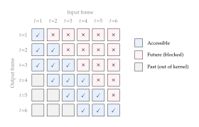
Let be a single-channel video tensor and a 3D convolution kernel, with the spatial half-widths as in Definition 12. The causal 3D convolution of with is defined as (Causal 3D CONV) The only change from (3D CONV) is the range of the temporal summation index: now runs over instead of , so that every tap has . The convolution therefore accesses only frames ; no future frame () is accessed. The spatial extents remain centred and two-sided: causality is a constraint on time alone.
In practice, causal 3D convolutions are implemented by applying asymmetric temporal padding: frames of zero-padding are prepended to the temporal dimension, and no padding is appended. This ensures that the output at time depends only on inputs at times , matching the standard causal convention used in autoregressive language models (17).
Example 13 (Implementation of Causal 3D Convolution).
In PyTorch, a causal 3D convolution with temporal kernel size
can be implemented by padding the input tensor with zero
frames along the temporal dimension at the start, and then applying a
standard nn.Conv3d with padding=(0, p_h, p_w)
(no temporal padding in the convolution itself, since we already
padded manually). Concretely:
Pad the input: along the time axis.
Apply the convolution: with symmetric spatial padding and zero temporal padding.
The output has the same temporal extent as , and each output frame depends only on input frames . This simple padding trick converts any standard 3D convolution into a causal one.
Proposition 7 (Causal Receptive Field Growth).
A stack of causal 3D convolutional layers, each with temporal kernel size and stride , produces a temporal receptive field of size (Causal Receptive) If temporal striding is used with stride at certain layers, the effective receptive field grows exponentially. Specifically, if all layers use stride , the receptive field becomes (Causal Receptive Strided) The geometric sum degenerates when , where it takes the value and (Causal Receptive Strided) reduces to (Causal Receptive), as it must. In either case, frame at the output depends only on frames at the input.
Proof.
For stride- layers, each layer extends the temporal receptive field by frames (the current frame plus past frames). Stacking layers yields .
For stride- layers, the -th layer (counting from ) operates on a temporal grid that has been downsampled by . Each step in this downsampled grid corresponds to steps in the original grid. The -th layer contributes frames to the receptive field; summing over all layers gives the geometric series, and the extra accounts for the single frame the receptive field already covers before any layer is applied.
Figure 9 illustrates the difference between causal and non-causal receptive fields for a stack of two layers with .
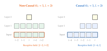
The Causal 3D-VAE Training Objective
With causal 3D convolutions as the building block, we can now define the full training objective for a causal 3D variational autoencoder. The objective follows the standard VAE framework (see 15) but is applied to video tensors with architectures that respect the causal constraint.
Theorem 2 (Causal 3D-VAE Evidence Lower Bound).
Let be a video tensor. Let be an encoder distribution parameterised by a causal 3D convolutional network with parameters , and let be a decoder distribution parameterised by . The evidence lower bound (ELBO) for the causal 3D-VAE is (Causal 3dvae ELBO) where is the standard Gaussian prior over latents, is a weighting coefficient (recovering the standard ELBO when ), and .
Proof.
The proof follows the standard VAE derivation (cf. 15). By Jensen's inequality applied to the log-marginal likelihood: (ELBO Derivation) The -weighted variant follows by replacing the KL coefficient with , as in the -VAE framework. The causality constraint enters through the architecture of : the encoder uses causal 3D convolutions, ensuring that the approximate posterior respects the causal structure.
In practice, the reconstruction term is evaluated using a Gaussian decoder, which reduces to a mean squared error: (Recon MSE) where denotes the Frobenius norm over all spatiotemporal dimensions and is a fixed noise variance (often set to ).
Remark 19.
The gap between the log-marginal likelihood and the ELBO equals the KL divergence between the approximate posterior and the true posterior: (ELBO GAP) This gap vanishes if and only if the approximate posterior exactly matches the true posterior. In practice, the gap is controlled by the expressiveness of the encoder architecture. Causal 3D encoders with large receptive fields can better approximate the true posterior than shallow encoders with small receptive fields, because they can capture long-range temporal dependencies in the posterior.
Example 14 (Reparameterisation for Causal 3D-VAE).
The reparameterisation trick (see 15) is applied to the causal 3D-VAE as follows. The encoder outputs two tensors: (the posterior mean) and (the log-variance). A latent sample is drawn as (Reparam) where denotes element-wise multiplication and . This reparameterisation allows gradients to flow through the sampling step, enabling end-to-end training of the encoder via backpropagation. The causality of the encoder ensures that and at temporal index depend only on input frames at indices , where is the temporal compression factor.
Temporal Compression Bound
How much temporal compression is achievable without destroying the video content? Intuitively, if consecutive frames are very similar (low motion), then aggressive temporal compression is possible. If frames change rapidly (high motion), compression must be more conservative. The following proposition makes this intuition precise.
Proposition 8 (Temporal Compression Bound).
Let be a video tensor reshaped so that each frame (with ) is a vector. Define the temporal autocorrelation at lag as (Temporal Autocorr) where is the temporal mean. Assume that the centred frames have a common norm, for every , and that is non-increasing over the lags . Suppose a temporal downsampling operator with factor (retaining every -th frame) is applied before encoding, and that each discarded frame is reconstructed by holding the most recently retained frame. Then the reconstruction error satisfies (Temporal Compression Bound) where is the reconstruction from the downsampled video. In particular, when (high temporal correlation across the whole downsampling window), the bound approaches zero and aggressive compression costs almost nothing. When (frames decorrelate within the window), the bound degenerates to : the entire signal energy of every discarded frame is at risk, and the achievable compression is correspondingly limited.
Proof.
The downsampled video retains frames at indices , so each discarded frame sits at some lag after the most recent retained frame , and the stated reconstruction sets . For centred frames of common norm , (Temporal Compression STEP) where is the summand of (Temporal Autocorr), whose average over is . Grouping the discarded frames by their lag, and taking to be a multiple of so that the classes are exact, each of the lag classes contains frames; averaging (Temporal Compression STEP) within each class and summing gives the last step using the assumed monotonicity of on . This is (Temporal Compression Bound).
Caution.
Two hypotheses are doing real work here. Autocorrelation functions are not monotone in general-a periodic signal such as a rotating wheel or a walking gait has an autocorrelation that rises again at the period-so the monotonicity assumption must be checked against the data rather than assumed. A real causal 3D-VAE also does far better than frame-holding, since it learns the interpolation; (Temporal Compression Bound) should be read as the error budget that a trained encoder has to beat, not as a description of what it achieves.
Remark 20.
In practice, modern causal 3D-VAEs use temporal compression (CogVideoX, Wan-Video) and temporal compression (some Open-Sora variants). The choice is guided by the typical temporal autocorrelation of the training data. Natural videos at 24 fps typically have ; under the exponentially decaying model of Proposition 2 this gives at the lag that actually governs compression, so the error budget of Proposition 8 remains small. Videos with rapid motion (sports, action scenes) may have lower autocorrelation, requiring either reduced compression or motion-adaptive encoding schemes.
The Complete Training Loss
The ELBO alone is insufficient for training a high-quality video autoencoder. Modern video autoencoders augment the ELBO with perceptual and adversarial losses that improve visual quality beyond what pixel-level reconstruction can achieve.
Definition 14 (Causal 3D-VAE Total Training Loss).
The total training loss for a causal 3D-VAE is (Total LOSS) where each component is defined as follows:
Reconstruction loss (pixel-level fidelity): (Recon LOSS) The norm is preferred over because it produces sharper reconstructions (the norm encourages blurry averages).
KL regularisation (latent space structure): (KL LOSS) For the standard diagonal Gaussian encoder , this has the closed-form expression (KL Closed)
Adversarial loss (perceptual sharpness): (ADV LOSS) where is a discriminator network trained to distinguish real videos from reconstructions . In practice, patch-based discriminators operating on individual frames or short clips are used.
Perceptual loss (feature-level similarity): (PERC LOSS) where extracts features from layer of a pre-trained network (typically a VGG or LPIPS network), and is a normalisation constant.
The hyperparameters , , and control the relative importance of each term. Typical values are (small, to avoid posterior collapse), , and .
Caution.
The KL weight requires careful tuning. Setting too high causes posterior collapse: the encoder learns to ignore the input and output the prior, producing latent codes that carry no information. Setting it too low produces a latent space with poor structure, making downstream diffusion training more difficult. The Stable Diffusion VAE uses ; video VAEs typically use similar or slightly larger values. See 15 for a detailed discussion of the posterior collapse phenomenon.
Encoder-Decoder Architecture
The encoder and decoder of a causal 3D-VAE follow the familiar hierarchical structure of image autoencoders, extended to three dimensions. Figure 10 shows a typical design.
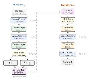
Example 15 (CogVideoX Causal 3D-VAE).
The CogVideoX model [17] uses a causal 3D-VAE with the following specifications:
Temporal compression factor: (49 input frames produce 13 latent frames).
Spatial compression factor: (height and width each reduced by a factor of 8).
Latent channels: .
Total compression ratio: .
Architecture: the encoder uses causal 3D convolutions with temporal kernel size and spatial kernel size . Temporal downsampling is achieved by strided convolutions with stride .
The first frame is encoded using purely spatial (2D) convolutions, ensuring compatibility with image inputs.
Example 16 (Wan-Video Causal 3D-VAE).
The Wan-Video model [7] uses a causal 3D-VAE with a similar design:
Temporal compression: .
Spatial compression: .
Latent channels: .
The model uses a “CausalConv3d” layer that applies frames of temporal padding on the left and zero padding on the right, ensuring strict causality.
Group normalisation is used throughout, with groups adapted for the increased channel dimensions.
The decoder mirrors the encoder architecture with transposed convolutions for upsampling.
Factorised Spatiotemporal Processing
Full 3D convolutions are parameter-heavy and computationally expensive. A common optimisation is to factorise each 3D convolution into separate spatial and temporal components.
Definition 15 (Factorised Spatiotemporal Convolution).
A factorised spatiotemporal convolution decomposes a 3D convolution with kernel into two sequential operations:
A spatial convolution with kernel that processes each frame independently.
A temporal convolution with kernel that processes each spatial location across time.
With causal padding applied to the temporal convolution, the factorised operation preserves the causal property while reducing the parameter count from to .
This factorisation was popularised by S3D [63] and R(2+1)D [64] in the video understanding literature and has been widely adopted in video generation. The Open-Sora [18] encoder uses this factorised design throughout, applying 2D spatial convolutions inherited from a pre-trained image autoencoder and adding temporal convolution layers that are trained from scratch.
Remark 21.
A practical advantage of the factorised design is that the spatial convolutions can be initialised from a pre-trained image autoencoder (such as the Stable Diffusion VAE), while only the temporal convolutions need to be trained from scratch. This “inflate and fine-tune” strategy dramatically reduces the amount of video data required for training and accelerates convergence.
Training Procedure
Training a causal 3D-VAE involves alternating between the autoencoder (encoder + decoder) and the discriminator, following the same adversarial training protocol used for image autoencoders.
Algorithm 3 (Causal 3D-VAE Training).
Input: Video dataset , encoder , decoder , discriminator , learning rate , loss weights . Output: Trained encoder and decoder .
Initialise spatial convolution weights from a pre-trained image autoencoder (e.g., Stable Diffusion VAE). Initialise temporal convolutions randomly.
For each mini-batch : enumerate[(a)]
Encode: for each .
Sample: , .
Decode: .
Compute losses: , , , as in Definition 14.
Update autoencoder: .
Update discriminator: , where . enumerate
Optional: Apply gradient penalty to stabilise discriminator training.
Remark 22.
In practice, training a causal 3D-VAE proceeds in stages. First, the autoencoder is trained without the adversarial loss () for a warm-up period of 10,000 to 50,000 steps, allowing the reconstruction and KL losses to stabilise. The discriminator is then introduced, and the adversarial loss is gradually increased to its final value. This staged approach prevents the discriminator from overwhelming the autoencoder in the early stages of training, when reconstructions are poor and the discriminator can trivially distinguish real from generated video.
Remark 23.
Several video autoencoders (CogVideoX, Open-Sora) train on a mixture of image and video data. Images are treated as single-frame videos and processed through the same encoder, with the temporal convolutions reducing to identity operations (since there is only one frame). This mixed training strategy ensures that the autoencoder retains strong per-frame reconstruction quality (inherited from the image data) while learning temporal compression (from the video data). Typical mixing ratios allocate 20–50% of mini-batch slots to images and the remainder to video clips.
Discrete Tokenisation for Video
The previous two sections developed continuous latent video autoencoders, where the latent space is a real-valued tensor . An alternative approach, rooted in the VQ-VAE framework (see 16), replaces the continuous latent space with a discrete one. Each spatial (or spatiotemporal) location in the latent tensor is mapped to the nearest entry in a learned codebook, producing a sequence of discrete tokens that represent the video.
Discrete tokenisation has a compelling appeal: it unifies video generation with the autoregressive language modelling paradigm that has proven so successful for text. Once a video is encoded as a sequence of discrete tokens, it can be modelled by a standard autoregressive transformer (GPT-style) or a masked transformer (BERT-style), inheriting the powerful sequence modelling capabilities developed for natural language processing.
Key Idea.
From pixels to tokens. Discrete video tokenisation bridges the gap between continuous visual signals and discrete sequence modelling. A video is mapped to a sequence of tokens where each indexes a learned codebook entry. This reduction, from millions of continuous pixel values to thousands of discrete tokens, enables the use of powerful autoregressive priors for video generation.
Vector Quantisation for Video
The foundation of discrete video tokenisation is vector quantisation (VQ), which maps continuous encoder outputs to the nearest entry in a finite codebook.
Definition 16 (Video Codebook).
A video codebook is a set of learnable vectors (Codebook) where is the embedding dimension and is the codebook size (typically to ). The quantisation operator maps a continuous vector to its nearest codebook entry: (Quantise)
For a video tensor, quantisation is applied independently to each spatiotemporal location in the latent tensor. The encoder produces , and each vector is quantised independently: (VQ Video) The resulting discrete token sequence has length , with each token taking values in .
Remark 24.
The compression achieved by VQ is substantial. Consider a video with frames at resolution. With temporal and spatial compression, the token sequence has length . With a codebook of size , each token requires bits, so the entire video is represented by bits, compared to bits in the raw pixel representation. This is a compression ratio of .
Training with the Straight-Through Estimator
The quantisation operator has zero gradients almost everywhere (and undefined gradients at the Voronoi boundaries). To train the encoder through the quantisation bottleneck, VQ-VAE [13] uses the straight-through estimator (STE): during the forward pass, the quantised values are used; during the backward pass, gradients are copied directly from the decoder input to the encoder output, bypassing the quantisation step: (STE) where denotes the stop-gradient operator. This expression evaluates to in the forward pass (since ) but has gradient in the backward pass (since the stop-gradient term contributes zero gradient).
The VQ-VAE training loss combines reconstruction with two commitment terms that keep encoder outputs and codebook entries close:
Definition 17 (VQ-VAE Training Loss for Video).
The VQ-VAE training loss for a video tokeniser is (VQ LOSS) where is the encoder output, is the quantised code, is the reconstruction, is the stop-gradient operator, and is the commitment cost coefficient (typically ).
The three terms serve distinct purposes. The reconstruction loss trains the decoder. The codebook loss moves codebook entries toward encoder outputs (training only the codebook, since the encoder output is stopped). The commitment loss moves encoder outputs toward codebook entries (training only the encoder, since the codebook entry is stopped). Together, they ensure that encoder outputs and codebook entries remain close, preventing codebook collapse (where large portions of the codebook go unused).
Caution.
Codebook collapse is a persistent challenge. In practice, a large fraction of codebook entries may never be selected during training, effectively reducing the codebook size. Several techniques mitigate this problem:
Exponential moving average (EMA) updates: Instead of gradient-based codebook updates, replace each codebook entry with an exponential moving average of the encoder outputs that are assigned to it: , where is the mean of encoder outputs assigned to entry and .
Codebook reset: Periodically replace unused codebook entries with randomly selected encoder outputs from the current batch, ensuring that all entries remain active.
Entropy regularisation: Add a term to the loss that encourages a uniform distribution over codebook assignments, where and denotes entropy.
Example 17 (Codebook Utilisation in Practice).
A well-trained video VQ-VAE with codebook entries typically achieves 60–90% codebook utilisation (meaning 4,900 to 7,400 entries are selected at least once per epoch). With EMA updates and periodic resets, utilisation can reach 95% or higher. MAGVIT-v2 [16] reported that without entropy regularisation, utilisation dropped below 20% for codebook sizes exceeding . With entropy regularisation, utilisation remained above 90% even for .
Lookup-Free Quantisation
A persistent challenge with standard VQ is that increasing the codebook size beyond a few thousand entries leads to codebook underutilisation: many codebook entries are never selected, wasting representational capacity. MAGVIT-v2 [16] introduced lookup-free quantisation (LFQ) to address this problem.
Definition 18 (Lookup-Free Quantisation).
Lookup-free quantisation (LFQ) replaces the explicit codebook with a simple sign function. Given an encoder output , the quantised representation is (LFQ) where is applied element-wise. The implicit codebook is the set of all vertices of the -dimensional hypercube , so the codebook size is with zero learnable codebook parameters.
LFQ eliminates the codebook collapse problem entirely: every “codebook entry” (vertex of the hypercube) is equally accessible, and utilisation is determined solely by the distribution of encoder outputs. The sign function is non-differentiable, but gradients can be estimated using a smooth approximation such as with , or by using the straight-through estimator.
Proposition 9 (LFQ Codebook Capacity).
With embedding dimension , LFQ provides a codebook of size using zero learnable parameters. The information carried by one quantised location is at most bits, with equality if and only if the sign bits are independent and each is uniformly distributed over ; bits is therefore the capacity of the location, not its realised rate. For , the codebook size is , vastly exceeding the typical VQ codebook sizes of to .
Proof.
Each dimension of the encoder output is quantised to , so the total number of distinct codes is and the entropy of the quantised location is at most bits. Equality in the entropy bound requires the uniform distribution over the hypercube vertices, that is, independent and unbiased sign bits; any correlation between the dimensions, or any bias in a single sign, strictly reduces the realised rate below bits. Since the codebook is defined implicitly by the sign function, no learnable codebook parameters are required.
Remark 25.
The gap between capacity and realised rate is exactly what the entropy regularisation of Example 17 is for. LFQ removes the mechanism of codebook collapse-there is no learned codebook left to collapse-but it does not by itself force the encoder to use the hypercube uniformly. A trained LFQ tokeniser still needs an entropy term to push the realised rate towards the -bit ceiling.
Example 18 (MAGVIT-v2 Video Tokeniser).
MAGVIT-v2 [16] uses LFQ with , giving an implicit codebook of entries. Combined with a causal 3D encoder using temporal and spatial compression, a -frame video at is tokenised into tokens, each drawn from a vocabulary of . This large vocabulary enables the model to represent fine visual details that would be lost with smaller codebooks. The resulting token sequence can be modelled by an autoregressive transformer, unifying video generation with language modelling.
Remark 26 (Continuous vs. Discrete Latent Spaces for Video).
The choice between continuous and discrete latent spaces reflects a fundamental trade-off in video generation:
Continuous latents (as in causal 3D-VAEs) enable gradient flow from the diffusion model through the latent space to the autoencoder, facilitating end-to-end fine-tuning. The smooth geometry of continuous spaces is well-matched to the Gaussian noise process of diffusion models.
Discrete tokens (as in VQ-VAE and LFQ) enable the use of autoregressive priors, which can model complex dependencies through next-token prediction. Discrete tokens also provide a natural interface for multimodal models that operate on mixed sequences of text and visual tokens.
In practice, the field has converged toward continuous latents for diffusion-based generation (Sora, CogVideoX, Wan-Video) and discrete tokens for autoregressive generation (VideoGPT, MAGVIT-v2, VideoPoet). Some systems use both: a continuous latent space for the diffusion process and discrete tokens for conditioning or planning.
The VQ-Video Pipeline
Figure 11 illustrates the complete VQ-based video tokenisation pipeline, from input frames through 3D encoding, quantisation, and decoding.
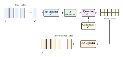
Example 19 (VideoGPT).
VideoGPT [2] was one of the earliest systems to combine VQ-VAE video tokenisation with an autoregressive transformer prior. The architecture consists of:
A 3D VQ-VAE with temporal and spatial downsampling, using axial attention in the encoder and decoder.
A codebook of entries with embedding dimension .
A GPT-2-style transformer that models the token sequence autoregressively, either unconditionally or conditioned on a class label or on given initial frames. VideoGPT has no text encoder; text conditioning arrived in later systems.
While VideoGPT's generation quality was limited by the small codebook and modest model scale, it demonstrated the viability of the “tokenise then model autoregressively” paradigm for video.
Latent Space Temporal Structure
The preceding sections developed the machinery for compressing video into a latent space, whether continuous (causal 3D-VAE) or discrete (VQ-based tokenisation). We now turn to a fundamental question: what properties does the latent space inherit from the temporal structure of the input video? Understanding this question is essential for designing diffusion models that generate temporally coherent video in latent space.
The central insight of this section is both simple and powerful: temporal smoothness in pixel space translates to temporal smoothness in latent space, provided the encoder satisfies mild regularity conditions. This means that if consecutive video frames are similar (as they almost always are in natural video), then their latent codes are also similar. The diffusion model can therefore generate smooth video by generating smooth trajectories in latent space.
Latent Temporal Lipschitz Continuity
We begin with the fundamental theorem connecting pixel-space smoothness to latent-space smoothness.
Theorem 3 (Latent Temporal Lipschitz Continuity).
Let be a video frame encoder that is -Lipschitz continuous with respect to the Frobenius norm: (Lipschitz Encoder) If consecutive video frames satisfy for all , then the corresponding latent codes satisfy (Lipschitz Latent) where . In particular, if the video is temporally smooth (), then the latent trajectory is also smooth, with smoothness scaled by the Lipschitz constant .
Two hypotheses should be read carefully. First, the encoder is applied frame by frame, so the theorem as stated describes the spatial-only autoencoder of Definition 8; Remark 28 gives the corresponding statement for a temporally mixing causal 3D encoder. Second, -Lipschitz continuity is an assumption on , not a property every network enjoys; see Remark 27.
Proof.
The proof is a direct application of the Lipschitz condition. For any consecutive frames and : (Lipschitz Proof STEP) where the first inequality uses the -Lipschitz condition on and the second uses the temporal smoothness assumption .
Remark 27.
Are neural network encoders Lipschitz continuous? Not automatically, and the exception matters here. A network built purely from Lipschitz layers-linear layers, convolutions, ReLU activations, and normalisation layers with fixed statistics-is itself Lipschitz continuous, with a Lipschitz constant bounded by the product of the operator norms of the weight matrices. For such a network with layers and weight matrices : (Lipschitz Network) where is the spectral norm of the -th weight matrix. (We write rather than for the depth because already denotes the Lipschitz constant in Theorem 3.)
The qualification is not pedantic. Softmax self-attention is not globally Lipschitz on an unbounded input domain, and the encoder drawn in Figure 10 contains exactly such an attention mid-block. What rescues the argument in practice is that video pixels are bounded: on a bounded input set, attention is Lipschitz, but with a constant that grows with the diameter of that set, so (Lipschitz Network) understates the true constant for any encoder containing attention. The honest reading of Theorem 3 is therefore conditional: if the encoder has a moderate Lipschitz constant on the region of pixel space where video actually lives, smooth video maps to smooth latents. Techniques such as spectral normalisation (Miyato et al., 2018 [19]) can be used to control the convolutional part of the bound; the attention block is normally left uncertified and its effective constant estimated empirically.
Remark 28 (Extension to causal 3D encoders).
Theorem 3 is stated for a per-frame encoder, so taken literally it describes the spatial-only autoencoder of Definition 8-precisely the design Causal 3D Variational Autoencoders argued against. The causal 3D-VAE mixes frames and reduces the frame count, so the statement needs adjusting.
Suppose the encoder is temporally translation-equivariant, as a convolutional encoder is away from the sequence boundary, so that every latent frame is produced by one and the same -Lipschitz local map applied to a window of consecutive input frames, and that the windows of consecutive latent frames are offset by the temporal compression factor . Each of the paired input frames is then at most steps apart, so it differs by at most , and (Lipschitz Latent 3D) Temporal smoothness still transfers, which is the load-bearing conclusion, but the constant is inflated by the compression factor and by the square root of the temporal receptive field. In the remainder of this section the trajectory index runs over the latent frames, and every bound of the form (Lipschitz Latent) should be read with the step bound replaced by (Lipschitz Latent 3D) whenever the encoder is a 3D one.
Corollary 2 (Latent Trajectory Diameter).
Under the conditions of Theorem 3, the total length of the latent trajectory satisfies (Trajectory Length) and the diameter of the trajectory (maximum distance between any two latent codes) satisfies (Trajectory Diameter) For a smooth video with and moderate , the latent trajectory is confined to a small region of the latent space, which the diffusion model can learn to navigate. The argument uses only the per-step bound, so it applies verbatim to a causal 3D encoder: if consecutive latent frames satisfy over latent frames, both the length and the diameter are at most .
Proof.
The trajectory length bound follows by summing (Lipschitz Latent) over . The diameter bound follows from the triangle inequality: .
First-Frame Conditioning
A common design pattern in video generation is to condition the diffusion model on the first frame of the video. The user provides an image, and the model generates a video that begins with that image and continues with plausible motion. This requires the autoencoder to treat the first frame specially.
Definition 19 (First-Frame Conditioning in Latent Space).
In first-frame conditioning, the latent representation of a video is decomposed as (First Frame) where encodes the first frame using an image encoder, and encodes the remaining frames using a video encoder (which may apply temporal compression). The semicolon denotes concatenation along the temporal axis.
This decomposition has several advantages. First, it allows the first frame to be encoded at full temporal resolution (no temporal compression), preserving the fine details of the conditioning image. Second, it enables the use of a pre-trained image encoder (such as the Stable Diffusion VAE) for the first frame, while using a video-specific encoder for the remaining frames. Third, during inference, the first frame's latent code can be provided as a fixed conditioning signal, and the diffusion model only needs to generate the remaining latent frames.
Example 20 (CogVideoX First-Frame Conditioning).
In CogVideoX [17], the causal 3D-VAE encodes the first frame using purely spatial (2D) convolutions, while subsequent frames are encoded using causal 3D convolutions with temporal compression. For a -frame input, the first frame produces latent frame, and the remaining frames produce latent frames, giving latent frames total. During image-to-video generation, the first latent frame is computed from the given image and held fixed, while the diffusion model generates only the remaining latent frames.
Remark 29.
First-frame conditioning creates a natural anchor point for temporal consistency. Because the first frame is encoded without temporal compression, its latent code faithfully represents the conditioning image. The diffusion model can then focus on generating motion and temporal evolution, knowing that the starting point is fixed. This separation of concerns (appearance from the first frame, motion from the diffusion model) simplifies the generation task and typically improves quality.
Latent Interpolation and Smooth Generation
The Lipschitz continuity theorem (Theorem 3) tells us that smooth videos produce smooth latent trajectories. The converse is equally important for generation: smooth latent trajectories should produce smooth videos. This motivates the study of latent interpolation.
Definition 20 (Linear Latent Interpolation).
Given two latent codes corresponding to two video frames, the linear interpolation at parameter is (Linear Interp) The decoded interpolation produces a frame that should visually interpolate between and .
Proposition 10 (Interpolation Smoothness).
If the decoder is -Lipschitz continuous, then the decoded interpolation path satisfies (Interp Smooth) for all . In particular, the decoded interpolation is Lipschitz continuous in with constant .
Proof.
The linear interpolation satisfies . Applying the Lipschitz condition on :
Definition 21 (Spherical Latent Interpolation).
For latent spaces where the norm carries semantic meaning (as in normalised or KL-regularised latent spaces), spherical linear interpolation (SLERP) often produces better results. Given unit-norm latent codes and with angle , the spherical interpolation is (Slerp) Unlike linear interpolation, SLERP maintains a constant norm along the interpolation path, avoiding the “norm dip” that occurs at with linear interpolation.
Remark 30.
The “norm dip” in linear interpolation deserves elaboration. For two unit-norm vectors and with angle between them, the norm of the linear interpolation at is (NORM DIP) When is large (distant points in latent space), this norm can be significantly less than , causing the decoded interpolation to pass through low-density regions of the latent space where the decoder has not been trained. SLERP avoids this by traversing the great circle on the unit sphere, maintaining for all . For VAE latent spaces where the prior is , the norm carries information about “typicality”: latent codes with norms far from (the expected norm of a -dimensional standard Gaussian) tend to produce poor-quality decoding.
Example 21 (Latent Interpolation for Video Frame Interpolation).
Latent interpolation provides a simple approach to video frame interpolation (generating intermediate frames between two given frames). Given frames and :
Encode both frames: , .
Interpolate in latent space at evenly spaced values: for , .
Decode the interpolated latents: .
This produces intermediate frames that smoothly transition from to . The quality of the interpolation depends on how well the latent space is structured: a well-structured VAE latent space produces semantically meaningful interpolations where objects move smoothly, while a poorly structured latent space may produce artefacts at intermediate values. Note that this is a property the KL term has to be tuned towards, from either side: too small a leaves the latent space unstructured, too large a one collapses it (cf. the warning following Definition 14).
Temporal Structure in the Latent Diffusion Process
The latent temporal structure has direct implications for the design of the diffusion model that operates in the latent space. Because the latent trajectory of a natural video is smooth (Theorem 3), the noise schedule and denoising architecture can be designed to exploit this smoothness.
Insight.
Temporal smoothness simplifies the diffusion task. Consider the noising process applied to a latent video . At noise level , the noised latent is , where . The denoising model must predict the noise (or equivalently, the clean latent ) from .
When has smooth temporal structure, the clean signal along the temporal dimension is low-frequency. The noise , being i.i.d. Gaussian, is high-frequency. This spectral separation makes the denoising task easier: the model can partially denoise by applying temporal smoothing, a much simpler operation than spatial denoising. This insight helps explain why video diffusion models often converge faster than one might expect given the high dimensionality of the latent space.
To formalise this, consider the temporal frequency content of the latent tensor. For a fixed spatial location and channel , the temporal signal is a one-dimensional sequence. Its discrete Fourier transform reveals the frequency content: (Latent FFT)
For a temporally smooth latent (small ), the energy is concentrated at low frequencies (, and equivalently , since the two ends of the DFT index range carry the same low frequency), while the noise has uniform spectral energy across all frequencies. The denoising model can exploit this asymmetry by attending to temporal patterns at different frequency scales.
Lemma 2 (Spectral Energy Concentration).
Let be a temporal signal satisfying for all , with indices read cyclically (so that as well). Recall that in the DFT convention of (Latent FFT) the index and the index carry the same physical frequency, so the genuinely high-frequency band is the one centred on . On that band, (Spectral Bound) and more generally, for any band , (Spectral Bound General) Since the total energy is , the fraction of the signal's energy sitting in the high band is at most , where is the mean square latent value. This ratio does not grow with : it is small precisely when the frame-to-frame change is small compared with the typical latent magnitude, which is the regime Theorem 3 delivers.
Proof.
The cyclic difference signal has for all . The DFTs of and are related by , and . By Parseval's theorem in this convention, For any band this gives , which is (Spectral Bound General). On the band the function attains its minimum at the two endpoints, where ; substituting gives (Spectral Bound). The energy-fraction statement follows by dividing by .
Latent Trajectories as Curves
A useful geometric perspective is to view the sequence of latent codes as a discrete curve in the latent space . This curve-based view provides intuitions for how the diffusion model generates video.
Definition 22 (Latent Video Trajectory).
The latent video trajectory of a video under encoder is the discrete curve (Latent Trajectory) where the are the latent codes obtained by encoding (and possibly temporally compressing) the input frames.
Figure 12 visualises this concept. For a natural video containing smooth motion (e.g., a camera pan or a walking person), the latent trajectory forms a smooth curve. For a video with abrupt scene changes (e.g., a cut between shots), the trajectory contains discontinuities.
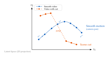
Implications for Diffusion Model Design
The temporal structure of the latent space has several important implications for the design of the diffusion model that operates within it.
Temporal attention is essential.
Because adjacent latent frames are correlated (as guaranteed by Theorem 3), the denoising model must attend across the temporal dimension to exploit these correlations. A model that processes each latent frame independently would ignore the most predictable structure in the data. This motivates the temporal attention mechanisms and 3D architectures developed in sec:vdiff:dit,sec:vdiff:factored-attn.
Noise scheduling can be temporal-aware.
The spectral concentration result (Lemma 2) suggests that temporal low-frequency components of the latent video should be denoised first (they contain the large-scale motion and scene structure), while high-frequency temporal details can be added later. This matches the coarse-to-fine generation observed in practice.
The diffusion model generates curves, not frames.
From the geometric perspective of Latent Trajectories as Curves, the diffusion model's task is not to generate independent latent frames but to generate a smooth curve in the latent space. This is a lower-dimensional problem than generating independent points, because the curve is constrained by temporal continuity.
Proposition 11 (Effective Dimensionality Reduction).
Let be a latent trajectory with for all , where each with and is the effective step bound of Theorem 3 or Remark 28. Every frame then lies within the ball of radius about , so the whole trajectory lies in a tube . Relative to the full latent hypercube this tube occupies a fraction (Volume Ratio) which is exponentially small in whenever . The diffusion model only needs to learn the distribution over this tiny fraction of the full latent space.
Proof.
By Corollary 2, applied with step bound over frames, every lies within the ball of radius in . Hence whose volume is at most , where is the volume of the unit ball in . Dividing by the cube volume gives and for all , so dropping it only weakens the bound. Note that the exponent is , not : it is the successive frames that are each confined, and the first frame that is free.
Latent Space Quality and Downstream Diffusion
The quality of the latent space directly affects the quality of the downstream diffusion model. A well-structured latent space has several desirable properties that simplify the diffusion task.
Definition 23 (Latent Space Desiderata for Video Diffusion).
A latent space produced by a video autoencoder is well-suited for diffusion if it satisfies:
Near-Gaussian marginals: The distribution of latent codes over the training set is approximately . This ensures compatibility with the standard Gaussian noise process used in diffusion.
Temporal smoothness: Consecutive latent frames and are close in distance, as guaranteed by Theorem 3 when the encoder is Lipschitz.
Semantic disentanglement: Different dimensions of the latent space encode semantically distinct aspects of the video (e.g., appearance vs. motion, foreground vs. background).
High reconstruction fidelity: The decoder faithfully reconstructs videos from latent codes, so that any video generated in latent space can be decoded to a high-quality pixel-space video.
Remark 31.
In practice, even with KL regularisation, the latent distribution may not be exactly standard Gaussian. A common post-processing step is to compute the per-channel mean and standard deviation of the latent codes over the training set, and normalise: . This ensures that the diffusion model operates on latents with approximately zero mean and unit variance, matching the assumptions of the standard noise schedule. Stable Diffusion, for instance, applies such a scaling factor (approximately ) to its latent codes before diffusion.
Exercise 10.
Consider a video autoencoder with the following specifications: input resolution at 24 fps for 4 seconds (96 frames), spatial compression , temporal compression , and latent channels.
Compute the total number of values in the input video tensor.
Compute the total number of values in the latent tensor.
What is the compression ratio?
If each value requires 16 bits (FP16), how much memory does the latent tensor require?
Exercise 11.
Let be an encoder consisting of 5 convolutional layers with spectral norms , , , , , using ReLU activations (which are -Lipschitz).
Compute an upper bound on the Lipschitz constant of .
If consecutive video frames differ by at most in Frobenius norm, what is the maximum distance between consecutive latent codes?
For a 24-frame video, what is the maximum diameter of the latent trajectory?
Exercise 12.
A video VQ-VAE uses a codebook of size with embedding dimension . The encoder produces a latent grid of shape (temporal height width) from a input video.
How many tokens represent the video?
How many bits of information does the token sequence carry?
Compare this to the number of bits in the raw video (assuming 8 bits per channel, 3 channels).
If a transformer models the token sequence autoregressively, what is the vocabulary size and sequence length?
Connecting Latent Compression to Video Diffusion
This section has established the mathematical foundations of latent space temporal structure. The key results can be summarised as follows:
Temporal smoothness transfers (Theorem 3): Lipschitz encoders map smooth pixel-space videos to smooth latent trajectories.
Spectral concentration (Lemma 2): smooth latent trajectories have energy concentrated at low temporal frequencies, creating a spectral separation between signal and noise that aids denoising.
First-frame conditioning (Definition 19): treating the first frame specially provides an anchor point for generation and enables image-to-video tasks.
Dimensionality reduction (Proposition 11): temporal smoothness constrains the latent trajectory to a small region of the full latent space, reducing the effective dimensionality of the generation problem.
Together, these results explain why latent video diffusion works as well as it does. The autoencoder compresses the video into a manageable latent space; the temporal structure of natural video ensures that the latent trajectories are smooth and low-dimensional; and the diffusion model exploits this structure to generate coherent video by tracing plausible curves through the latent space.
The next five sections build on this foundation to develop the architecture of the diffusion model that runs inside the latent space. The Diffusion Transformer (Video Diffusion Transformer (DiT)) is designed to process spatiotemporal latent tensors, cutting them into spacetime patches and modulating each block by the diffusion timestep. Because full spatiotemporal attention over those patches is unaffordable, Factored Attention for Video factorises it into spatial and temporal passes-the mechanism that exploits, at the level of the architecture, exactly the temporal smoothness established here. 3D Positional Encoding supplies the 3D positional encodings that tell those attention layers where in space and time each token sits, and Conditioning Mechanisms develops the conditioning pathways, including the concatenation route that carries the first-frame anchor of Definition 19 into image-to-video generation. Mixture-of-Experts for Video closes the architectural pillar by buying back capacity with mixture-of-experts layers. Only then, with an architecture in hand, do we return to the training objective and the noise schedule.
Video Diffusion Transformer (DiT)
The latent video diffusion framework developed in the preceding sections requires a neural network backbone that can process spatiotemporal latent tensors and predict either the noise , the clean data , or the velocity field at each denoising step. Early video diffusion models inherited the U-Net architecture from image diffusion, inflating 2D convolutions to 3D and inserting temporal attention layers between spatial blocks. While functional, this approach suffers from several limitations: the U-Net's hierarchical structure complicates scaling, the interleaving of convolution and attention creates architectural heterogeneity, and the inductive biases of convolution (locality, translation equivariance) may be unnecessarily restrictive for a model that already operates in a compressed latent space.
The Diffusion Transformer (DiT), introduced by Peebles and Xie [9] for images and subsequently extended to video by multiple groups, replaces the U-Net entirely with a plain transformer. The key insight is that, after latent compression, the effective resolution is small enough that a transformer operating on patch tokens can match or exceed U-Net performance while offering superior scaling behaviour.
In this section, we develop the DiT architecture for video from first principles. We begin with the spatiotemporal patchification that converts a latent tensor into a token sequence, then describe the adaptive layer normalisation mechanism that conditions the transformer on the diffusion timestep, and finally compare the scaling properties of DiT and U-Net architectures.
Spatiotemporal Patchification
The first step in processing a latent video tensor with a transformer is to convert the 3D grid of latent values into a 1D sequence of tokens. This is accomplished by dividing the tensor into non-overlapping 3D patches and projecting each patch to a token vector.
Definition 24 (Spatiotemporal Patchification).
Let be a latent video tensor. Choose patch sizes along the temporal, height, and width axes, respectively. The spatiotemporal patchification operator divides into non-overlapping 3D patches of size and flattens each patch into a vector: (Patchify) where the number of tokens is (NUM Tokens) Each patch vector is then projected to the model's hidden dimension via a learnable linear map : (Patch Embed) where is a positional embedding encoding the 3D location of patch (see 3D Positional Encoding).
The patchification process is illustrated in Figure 13. Note the analogy with the Vision Transformer (ViT): just as ViT converts a 2D image into a sequence of 2D patch tokens, the video DiT converts a 3D latent tensor into a sequence of 3D patch tokens. The critical difference is that each patch spans multiple frames, so the initial token embedding already captures local spatiotemporal structure.
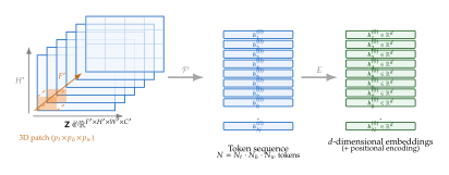
Example 22 (Token count for a typical video DiT).
Consider a latent tensor of shape , obtained from a temporal and spatial compression of a -frame, video. With patch sizes , , , the number of tokens is Each patch vector has dimension . With a hidden dimension of , the patch embedding matrix has parameters.
With larger patch sizes , , , the token count drops to , a reduction at the cost of coarser temporal granularity in the initial embedding.
Remark 32.
The choice of patch sizes involves a fundamental trade-off. Larger patches reduce the token count and hence the quadratic attention cost , but each token covers a larger spatiotemporal region, reducing the model's ability to capture fine-grained details. In practice, the temporal patch size is the most impactful parameter because it directly controls the temporal resolution of the token sequence. Most contemporary video DiT models use to preserve temporal detail, while using moderate spatial patches .
Proposition 12 (Patchification as strided convolution).
The spatiotemporal patchification operation of Definition 24 is equivalent to a 3D convolution with kernel size , stride , and output channels, applied to the latent tensor : (Patch AS CONV) where the convolution weight tensor encodes the same linear map as the embedding matrix .
Proof.
The convolution output at spatial position is This is exactly the inner product of the weight tensor (reshaped as a matrix of size ) with the flattened patch at position , which is the definition of the patch embedding . The stride ensures non-overlapping coverage.
The DiT Block with Adaptive Layer Normalisation
After patchification, the token sequence is processed by a stack of transformer blocks. Each block follows the standard pre-normalisation transformer design (LayerNorm, Attention, LayerNorm, MLP), but with a critical modification: the layer normalisation is adaptive, conditioned on the diffusion timestep and optionally on other global conditioning signals.
Definition 25 (Adaptive Layer Normalisation (adaLN)).
Let be a hidden representation, and let be the diffusion timestep. The adaptive layer normalisation (adaLN) is defined as (Adaln) where and are the mean and standard deviation computed over the feature dimension, is a small constant for numerical stability, and the adaptive scale and shift parameters are predicted from the timestep embedding: (Adaln Params) where is a sinusoidal or learnable timestep embedding and the predicts both parameters jointly.
Key Idea.
Timestep conditioning via normalisation. In a diffusion model, the network must behave differently at different noise levels: at high noise (), the model must make coarse, global predictions; at low noise (), it must refine fine details. AdaLN provides a lightweight mechanism for this adaptation by modulating the feature statistics at every layer. Rather than concatenating the timestep as an extra input token (which would require the attention mechanism to learn how to extract this information), adaLN directly controls the scale and shift of every feature channel, enabling the network to smoothly interpolate between different “operating modes” as a function of .
The full DiT block combines adaLN with multi-head self-attention (MHSA) and a position-wise feed-forward network (FFN), using the adaLN-Zero initialisation strategy.
Definition 26 (DiT Block with adaLN-Zero).
Let denote the token representations at layer . The DiT block at layer computes (DIT ATTN) where are gating parameters predicted from the timestep embedding alongside and : (Adaln ZERO Params) The adaLN-Zero initialisation sets the final linear layer of each to zero at the start of training, so that initially. This causes the DiT block to act as the identity function before any learning occurs.
Insight.
Why zero initialisation helps. At initialisation, the residual branches contribute nothing, so the forward pass is simply a chain of identity mappings. This has two benefits. First, gradients flow freely through the network from the start of training, avoiding the vanishing gradient problems that can afflict deep transformers. Second, the model begins by “doing nothing” and gradually learns to apply increasingly complex transformations, which provides a natural form of curriculum learning. This is particularly important for video DiT models, which often have to layers and would otherwise be difficult to train.
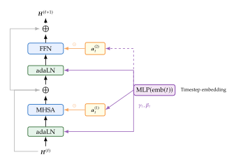
Mathematical Analysis of adaLN
To understand why adaLN is an effective conditioning mechanism, we analyse its effect on the feature distribution at each layer.
Lemma 3 (adaLN as affine feature modulation).
Let have mean and standard deviation across its components, and write for the layer-normalised vector, so that and . Then the mean of across the feature index is exactly (Adaln MEAN) If, in addition, the channel-indexed sequences , and are empirically uncorrelated across , in the sense that (Adaln Decorrelation) then (Adaln VAR) where mean and variance are taken over the feature dimensions. Under these hypotheses the output statistics are set by alone, independently of the input statistics .
Proof.
Layer normalisation guarantees and , which gives (Adaln MEAN) immediately by averaging over . Note that the cross-term does not vanish in general: it is the empirical covariance of and across channels, and it vanishes exactly when is constant across channels or is uncorrelated with .
For the variance, write and collect these into , so that the output is and , all moments being empirical over . The first hypothesis in (Adaln Decorrelation) makes , the second gives , and the third makes . Combining the three yields (Adaln VAR).
Proposition 13 (What adaLN conditioning can and cannot express).
Let denote standard layer normalisation, restricted to the set .
(Pointwise expressiveness is vacuous.) Fix a single and let be arbitrary. Then has a solution for every , namely . At a single input, adaLN can therefore produce any output whatsoever, and no expressiveness claim can be read off from one input.
(Uniform expressiveness is exactly the affine class.) Fix and let . A function satisfies on all of if and only if is the element-wise affine map composed with . In particular no choice of can mix feature coordinates or act non-affinely on .
Proof.
(i) is the displayed solution formula. For (ii), the “if” direction is immediate. For the converse, acts independently on each coordinate, , so if on then depends on only through and does so affinely, with the stated coefficients.
Remark 33 (Reading the proposition correctly).
It is tempting to argue that because are themselves predicted, adaLN is a universal per-channel transformation. That argument does not apply here: by (Adaln Params) the parameters are functions of the timestep embedding and of any other global conditioning signal, not of the token feature . For a fixed every token in the sequence is modulated by the same , so Proposition 13(ii) applies verbatim: as a function of its input, an adaLN layer is a per-channel affine map and nothing more. All input-dependent mixing in a DiT block is performed by the attention and feed-forward sub-layers; adaLN's role is to supply a cheap, global, -dependent gain and offset that steers those sub-layers. This is also why the practical benefit of adaLN-Zero is an optimisation benefit rather than an expressiveness one: as Definition 26 shows, zeroing the gates makes the whole block the identity at initialisation, which is a statement about the shape of the loss landscape at step zero, not about which functions the block can ultimately represent.
Comparison with U-Net Architectures
The shift from U-Net to DiT for video diffusion is not merely an architectural preference; it reflects fundamental differences in how the two architectures scale with model size and data.
Remark 34 (Structural differences).
The U-Net architecture consists of an encoder path that progressively downsamples the spatial resolution, a bottleneck, and a decoder path that upsamples with skip connections from the encoder. Each level operates at a different resolution, and the skip connections enable fine-grained spatial detail to bypass the bottleneck. The DiT, by contrast, operates at a single resolution throughout (the patch token resolution) and relies on self-attention to capture both local and global dependencies.
Proposition 14 (Parameter scaling comparison).
Consider a U-Net with levels, base channels (doubling at each level), and residual blocks per level. The total parameter count scales as (UNET Params) which grows exponentially with depth. A DiT with blocks, hidden dimension , and attention heads has parameter count (DIT Params) which grows linearly in depth and quadratically in width. The DiT offers a more predictable and controllable scaling behaviour.
Proof.
For the U-Net, at level the channel count is . Each residual block contains two convolutions of size (for kernel size ), giving per-level cost . Summing over levels yields the geometric series. For the DiT, each block has: (i) QKV projections costing , (ii) output projection , (iii) FFN with two layers , where typically . Total per block is , giving overall.
Example 23 (Scaling comparison in practice).
tab:vdiff:dit-unet compares representative configurations. The DiT achieves comparable or superior performance with more predictable compute-performance trade-offs.
tableComparison of U-Net and DiT architectures at similar
parameter counts. GFLOPs are computed per denoising step for a
single latent frame, which at patch
size gives tokens; these are the
image-domain reference configurations of Peebles and
Xie [9]. A video latent of such frames
multiplies the FFN and projection cost by and, under full
spatiotemporal attention, multiplies the attention cost by
.
Architecture Params GFLOPs Depth Width U-Net-S (3 levels, ) 400M 85 3 128–512 U-Net-L (4 levels, ) 1.2B 310 4 192–1536 DiT-B (, ) 130M 42 12 768 DiT-L (, ) 460M 145 24 1024 DiT-XL (, ) 675M 220 28 1152 DiT-G (, ) 1.8B 620 40 1536
Historical Note.
The Diffusion Transformer was introduced by Peebles and Xie [9] in 2023 for class-conditional image generation. Their key contribution was showing that, contrary to prevailing wisdom, a plain transformer without convolutional components could outperform U-Net architectures when properly scaled. The adaLN-Zero conditioning mechanism was inspired by film [20] (Feature-wise Linear Modulation) and earlier work on conditional normalisation in GANs. The extension to video was pursued independently by several groups, most notably in Open-Sora [18], Latte [21], and the architecture underlying Sora [6]. The U-ViT architecture of Bao et al. [22] explored a related but distinct design that adds skip connections between transformer layers, creating a U-Net-like structure within a transformer.
Exercise 13.
Consider a video DiT with layers, hidden dimension , attention heads, and FFN hidden dimension . The input latent tensor has shape with patch sizes , , .
Compute the number of tokens .
Compute the total number of parameters (ignoring the timestep embedding MLP).
Estimate the FLOPs for the self-attention operation in a single layer (both the product and the attention-weighted value computation).
How does the total attention FLOP count compare to the FFN FLOP count?
Exercise 14.
Consider the adaLN-Zero initialisation from Definition 26.
Show that when for all layers, the full -layer DiT computes .
Compute the Jacobian at initialisation and verify it is the identity.
Explain why this property facilitates gradient flow during the early stages of training.
Compare with the standard Xavier/He initialisation: what happens to gradient norms in a 40-layer transformer without adaLN-Zero?
Factored Attention for Video
The self-attention mechanism is both the greatest strength and the primary computational bottleneck of the video Diffusion Transformer. Given a token sequence of length , standard multi-head self-attention has time and memory complexity and , respectively, where is the hidden dimension and is the number of heads. For video, the token count is the product of temporal, height, and width dimensions, which can easily reach tens of thousands. Full spatiotemporal attention over all tokens is often computationally prohibitive, motivating the development of factored attention strategies that decompose the joint spatiotemporal attention into smaller, more manageable operations.
In this section, we analyse the computational cost of full spatiotemporal attention, develop the mathematical framework for factored attention, prove approximation bounds, and describe practical variants including joint attention and windowed attention.
Full Spatiotemporal Attention
We begin by quantifying the cost of the naive approach: computing attention over all video tokens simultaneously.
Definition 27 (Full Spatiotemporal Attention).
Let be the matrix of token representations, where each token corresponds to a spatiotemporal position . The full spatiotemporal attention computes (FULL ST ATTN) where , , are the query, key, and value projections, and is the per-head dimension.
Proposition 15 (Cost of full spatiotemporal attention).
The computational cost of full spatiotemporal attention for a single head on tokens with per-head dimension is:
QKV projections: FLOPs.
Attention matrix: FLOPs to compute .
Softmax: FLOPs.
Value aggregation: FLOPs to compute the weighted sum.
Memory: to store the attention matrix (or with FlashAttention, at the cost of recomputation).
The dominant cost is the term from the attention matrix computation.
Example 24 (Infeasibility of full attention for video).
For the latent tensor from Example 22 with tokens and (from with heads), the attention matrix has entries. In FP16, storing this matrix requires approximately GB per head, or GB for all 16 heads. The FLOPs for a single attention layer exceed , making full attention impractical for real-time or even batch training at this scale.
By contrast, with the reduced token count (using ), the attention matrix has entries, roughly a reduction, but still requiring careful memory management.
Caution.
Full spatiotemporal attention has complexity, which grows as the sixth power of the spatiotemporal resolution (since , , ). This scaling is fundamentally incompatible with the goal of generating high-resolution, long-duration video. Even with FlashAttention reducing the memory from to , the FLOPs remain quadratic and become the dominant bottleneck for sequences beyond a few thousand tokens.
Spatial-Then-Temporal Factorisation
The key observation that enables efficient video attention is that the spatiotemporal token grid has inherent structure: tokens at the same spatial location across different frames are temporally related, while tokens within the same frame are spatially related. Factored attention exploits this structure by decomposing the joint attention into separate spatial and temporal operations.
Definition 28 (Spatial-Then-Temporal Factored Attention).
Let be the token representations, reshaped so that the first axis indexes time and the second indexes spatial position. The spatial-then-temporal factored attention computes:
Step 1 (Spatial attention): For each temporal index , compute self-attention over the spatial tokens within frame : (Spatial ATTN) where are the query, key, and value matrices for frame .
Step 2 (Temporal attention): For each spatial index , compute self-attention over the temporal tokens at position : (Temporal ATTN) where are projections of the spatially-attended tokens at spatial position across all frames.
Proposition 16 (Cost of factored attention).
The computational cost of spatial-then-temporal factored attention is:
Spatial attention: independent attention operations, each over tokens, costing in total.
Temporal attention: independent attention operations, each over tokens, costing in total.
Total: (Factored Total COST)
Proof.
Each spatial attention for a single frame processes tokens with an attention matrix, requiring FLOPs. There are frames, giving . Similarly, each temporal attention at a single spatial position processes tokens, requiring , and there are positions, giving . The total is the sum.
Example 25 (Speedup from factorisation).
Using the token counts from Example 22: , , , so and .
Full attention cost (ignoring ): .
Factored attention cost: .
The speedup factor is approximately . For longer videos with , the speedup exceeds .
The factored attention achieves dramatic computational savings, but at a cost: information can only flow between spatially distant positions in different frames indirectly, through the composition of spatial and temporal attention. It is tempting to try to bound the resulting error against full attention, and it is worth being precise about why no useful bound of that kind exists.
Caution.
Factorisation is a restriction, not an approximation. Factored attention is often described as “approximating” full attention. It does not, in any sense that can be made quantitative a priori. Two observations make this concrete. First, an inequality such as is useless without a scale: every row of a softmax attention matrix is a probability vector, so for any two attention matrices every entry of lies in and each row of has norm at most , whence and automatically. A bound that exceeds says nothing at all. Second, the sequential composition is not obtained from by deleting entries: it is a different operator built from a different (and, in the alternating design of Alternating Block Design, differently parameterised) pair of projections. There is no free parameter one can send to zero to recover full attention. Factored attention is best understood as a restriction of the hypothesis class justified by the cost analysis of Proposition 16 and by empirical performance, not as a controlled approximation.
What can be stated cleanly is the effect of one specific operation: masking the cross terms inside a single attention layer and renormalising. This is the “axial” attention pattern in which each query attends to its own frame and its own spatial column, and it is the closest single-layer object to the factorisation.
Proposition 17 (Error of axial masking within one layer).
Fix a query index and let be the -th row of the full attention matrix . Let be the set of key indices that differ from in both spatial and temporal position, and let (Cross MASS) be the attention mass that full attention places on those pairs. Let be the row obtained by zeroing the entries in and renormalising. Then (Axial MASK Bound)
Proof.
By construction for and otherwise, so . The output difference is , whose norm is at most .
Remark 35.
Proposition 17 is only as strong as its hypothesis: the error is small precisely when the trained model's full attention already concentrates its mass on the same-frame and same-column slices, that is, when . That is an empirical property of trained video models, not a theorem, and it is plausible for natural video because tokens far apart in both space and time tend to have low mutual relevance - a patch showing sky in frame 1 interacts weakly with a patch showing ground in frame 20. Where it fails - fast camera motion, large object displacement, long-range occlusion reasoning - factored models are known to degrade, which is exactly why several recent systems have paid the quadratic price and returned to full 3D attention. The honest summary is that factorisation buys a large, provable saving in cost (Proposition 16) in exchange for an unprovable but empirically small loss in quality.
Alternating Block Design
In practice, factored attention is implemented by alternating between spatial attention blocks and temporal attention blocks. Each block is a full DiT block (Definition 26) with the attention restricted to a subset of tokens.
Definition 29 (Alternating Spatial-Temporal Transformer).
An alternating spatial-temporal transformer with total layers consists of spatial layers interleaved with temporal layers (assuming is even): (Alternating) where performs attention only within each frame (over tokens) and performs attention only across frames at each spatial position (over tokens). Both types of block include their own adaLN conditioning, attention, and FFN sub-layers.
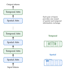
Lemma 4 (Information propagation in alternating attention).
In an alternating spatial-temporal transformer, spatial attention is global within a frame and temporal attention is global across frames at a fixed spatial position. Consequently, for every ordered pair of token positions and (writing for the flattened spatial index), a single spatial layer followed by a single temporal layer already provides a path from to . The effective receptive field of the alternating design therefore covers the entire token grid after one spatial-temporal pair, that is, after two layers.
Proof.
In the spatial layer, attends over its own frame, so it can influence the token - the token in 's frame at 's spatial position. In the following temporal layer, attends over the temporal column at spatial position , which contains . Composing the two gives a length-two path from to . The choice is always available because spatial attention is unrestricted within the frame, so no further layers are required.
Remark 36 (Connectivity is not the same as capacity).
Lemma 4 says that two layers suffice for every pair of tokens to be connected; it does not say that two layers suffice to model their interaction well. The path constructed in the proof is forced through the single intermediate token , whose -dimensional representation must carry, in superposition, whatever frame has to say to every other frame at that spatial position. Depth in an alternating stack therefore buys bandwidth and non-linearity for these interactions rather than reach. This is a genuine contrast with the windowed designs of 3D Window Attention, where connectivity itself is depth-limited and grows only as fast as Proposition 19 allows.
Joint Attention with Text Tokens
Not every design in this section restricts the attention graph; this one enlarges it. Joint attention, used in models such as CogVideoX [17], concatenates the text tokens with the video tokens and runs one attention over the combined sequence, rather than relegating text to a separate cross-attention mechanism. It is important to be clear that this is not a saving: the cost is quadratic in the combined length , strictly more than the of video self-attention alone. Joint attention is adopted for the quality of the text-video interaction it enables, and it is affordable only because .
Definition 30 (Joint Video-Text Attention).
Let be the video token representations and be the text token representations (obtained from a text encoder). The joint attention operates on the concatenated sequence: (Joint Concat) Self-attention is computed over this combined sequence: (Joint ATTN) where queries, keys, and values are computed from the full concatenated sequence. After attention, the text and video representations are separated and processed by their respective FFN layers.
Remark 37.
Joint attention differs from cross-attention in that text tokens can attend to video tokens (and vice versa), and text tokens can attend to each other. This bidirectional information flow allows the text representation to be refined based on the current state of the video generation, enabling more nuanced text-video alignment. In cross-attention, by contrast, the text representation is fixed and only influences the video tokens, with no feedback path. The trade-off is computational: joint attention with tokens costs , while separate cross-attention costs . When (typical: while ), the overhead of joint attention is modest because . Note that this is an overhead, not a saving: joint attention is strictly more expensive than video self-attention alone, and it is chosen for the quality of the interaction rather than for efficiency.
Example 26 (CogVideoX and the “expert transformer”).
CogVideoX [17] is frequently described as running text and video in two separate streams that are merged later, with the separation motivated as a way of avoiding attention that is quadratic in the combined sequence length. That description is wrong on both counts, and it is worth stating what the architecture actually does, because the design is a clean instance of Definition 30.
Text tokens and video tokens are concatenated into a single sequence and passed through a single full 3D self-attention at every block, exactly as in (Joint ATTN). The attention cost is therefore - it is quadratic in the combined length, and nothing about the design avoids that. What is modality-specific is the normalisation: the adaptive layer normalisation of Definition 25 uses one set of parameters for text tokens and a second, independent set for video tokens. This is the “expert adaptive layer norm” from which the name “expert transformer” derives, and its purpose is statistical, not computational: a frozen text encoder and a noised video latent have very different feature scales, and forcing a single normalisation to serve both makes the joint attention logits badly conditioned. Note also that the two “experts” here have nothing to do with the mixture-of-experts routing of Mixture-of-Experts for Video: there is no router, and the assignment of a token to an expert is fixed by its modality.
Proposition 18 (Effective conditioning strength).
In joint attention, the influence of text token on video token at layer is given by the attention weight (Joint Weight) The total text influence on video token is , and the output is (Joint Decompose) which is a convex combination of a text-conditioned component and a video self-attention component, with mixing coefficient that is learned end-to-end.
Proof.
The attention weights sum to 1 over all tokens by the softmax normalisation. Partitioning the sum into text indices and video indices gives the decomposition directly. The conditional distributions and are valid probability distributions over text and video tokens, respectively.
3D Window Attention
A complementary approach to factored attention is to restrict attention to local 3D windows, analogous to the Swin Transformer for images.
Definition 31 (3D Window Attention).
Partition the token grid of shape into non-overlapping 3D windows of size . Within each window, compute standard self-attention over the tokens: (Window ATTN) where is a learnable relative position bias. The total cost is (Window COST) which is linear in the total token count .
Definition 32 (Shifted 3D Window Attention).
To enable cross-window communication, alternate between regular and shifted window partitions: (Shifted Window) In the shifted configuration, each window overlaps portions of up to windows of the regular partition, one for each choice of “before or after” the shift along the three axes. A masking mechanism ensures that tokens from different logical regions do not attend to each other within boundary windows, preserving the local attention structure while enabling cross-boundary information flow.
Proposition 19 (Receptive field growth with shifted windows).
Consider a stack of window-attention layers in which regular and shifted partitions alternate, and let denote the number of shifted layers traversed - equivalently, the number of regular/shifted pairs, so that a network of such layers has . The effective receptive field of each token then spans (Shifted RF) tokens. For a 28-layer network with window size we have , and the receptive field reaches , which exceeds typical token grid sizes.
Proof.
Only the shifted layers enlarge the receptive field: a regular layer re-uses the same partition boundaries as the last regular layer, so it adds no new cross-boundary contacts. At each shifted layer the window boundary moves by , so a token at the edge of its current window gains access to tokens that lay in the adjacent window of the previous partition, extending its reach by the shift amount along each axis. After shifted layers the total extension is times the shift in each dimension, added to the initial window size.
Exercise 15.
Consider a video DiT whose token grid is , , , with per-head dimension . (These dimensions are chosen so that the window partition below tiles the grid exactly: , and .) Count FLOPs for an attention over tokens, covering both the product and the attention-weighted value computation.
Compute the FLOPs for full spatiotemporal attention (single head, single layer).
Compute the FLOPs for spatial-then-temporal factored attention.
Compute the FLOPs for 3D window attention with . Verify first that the windows tile the grid with no remainder, and say what would have to change if were instead of .
Rank the three approaches by FLOP count and discuss the quality-efficiency trade-off.
Exercise 16.
A video DiT uses joint attention with video tokens and text tokens, with hidden dimension and heads.
Compute the attention matrix size for joint attention vs. separate self-attention plus cross-attention.
What fraction of the joint attention FLOPs are “wasted” on text-to-text attention?
At what ratio does the overhead of joint attention exceed ?
Argue that the text self-attention in joint attention is not truly “wasted” because it enables text refinement conditioned on video state.
3D Positional Encoding
Transformers are permutation-equivariant by design: without positional information, a transformer cannot distinguish between a token representing the top-left corner of frame 1 and a token representing the bottom-right corner of frame 50. For video generation, positional encoding is not merely a technical detail; it is the mechanism by which the model understands the fundamental distinction between spatial and temporal relationships.
In this section, we develop three approaches to 3D positional encoding: the direct extension of sinusoidal encodings to three axes, Rotary Position Embeddings (RoPE) adapted to 3D grids, and learnable positional embeddings. We analyse the extrapolation properties of each approach and discuss their implications for generating videos at resolutions and durations not seen during training.
Why Position Matters for Video
To appreciate the importance of positional encoding, consider what a video DiT would produce without it.
Key Idea.
Without positional encoding, the transformer sees an unordered bag of patches. Consider a video of a ball moving from left to right. After patchification, two patches that are spatially adjacent in frame 5 are indistinguishable (from the transformer's perspective) from two patches that are temporally adjacent at the same spatial location in frames 5 and 6. The model cannot determine whether two tokens are neighbours in space or in time, whether one token comes before or after another in the video, or whether two similar-looking patches are at the beginning or end of the clip. Positional encoding resolves all of these ambiguities by injecting explicit location information into each token.
Formally, each token in the video DiT corresponds to a 3D grid position where , , and . The positional encoding must map this triple to a -dimensional vector (or a modification of the attention computation) that enables the transformer to reason about spatiotemporal relationships.
Definition 33 (3D Positional Encoding).
A 3D positional encoding is a function (3D PE General) that assigns a unique -dimensional vector to each grid position. The encoding is additive if it is summed with the patch embedding: , and rotary if it modifies the attention computation via rotation matrices (see 3D Rotary Position Embeddings (RoPE)).
3D Sinusoidal Positional Encoding
The simplest approach extends the classical 1D sinusoidal encoding of Vaswani et al. to three independent axes.
Definition 34 (3D Sinusoidal Positional Encoding).
Partition the embedding dimension into three groups of sizes , , with . For each axis, define the 1D sinusoidal encoding as (SIN 1D) where is a temperature parameter (typically ), is the dimension allocated to that axis, and . The 3D sinusoidal encoding is the concatenation: (3D SIN) where denotes concatenation.
Proposition 20 (Inner product structure of 3D sinusoidal PE).
The inner product between two 3D sinusoidal positional encodings decomposes as (SIN IP) where , , , and each function depends only on the relative displacement along its axis: (SIN Kernel) In particular, the inner product is translation-invariant along each axis: it depends only on relative displacements, not absolute positions.
Proof.
By the product-to-sum identity, for each frequency , Summing over all frequencies and all three axes gives the decomposition. Translation invariance follows because each depends on only.
Remark 38.
The additive decomposition means that the sinusoidal encoding cannot capture interactions between spatial and temporal positions. For example, the encoding cannot distinguish between “same spatial position, different frame” and “different spatial position, same frame” when the respective values happen to coincide. This limitation motivates the use of more expressive encodings such as RoPE.
3D Rotary Position Embeddings (RoPE)
Rotary Position Embeddings (RoPE), introduced by Su et al. [65], encode positional information by rotating query and key vectors in the attention computation. The 3D extension applies independent rotations for each spatial and temporal axis.
Definition 35 (1D Rotary Position Embedding).
Given a vector and position , the Rotary Position Embedding applies a block-diagonal rotation matrix: (ROPE 1D) where is block-diagonal with rotation blocks: (ROPE Block) with frequency parameters for base temperature .
Lemma 5 (Relative position property of RoPE).
For any positions and vectors , (ROPE Relative) so the attention logit depends only on the relative position .
Proof.
Since each is an orthogonal matrix, . Therefore, , where the last equality uses the group property .
Definition 36 (3D RoPE for Video).
Partition the per-head dimension into three groups of sizes , , with . The 3D RoPE for a token at position applies independent rotations to each group of dimensions: (3D ROPE) where are rotation matrices as in (ROPE Block), potentially with different base temperatures for each axis.
Theorem 4 (Factored relative position in 3D RoPE).
The attention logit under 3D RoPE decomposes as a sum of per-axis contributions: (3D ROPE Logit) where etc., and each depends on the relative displacement along that axis and the content of the query and key vectors in the corresponding dimension group.
Proof.
Since the three groups of dimensions are disjoint, the inner product decomposes as , where each term uses Lemma 5 applied to the respective axis.
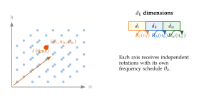
Resolution and Length Generalisation
A critical practical question is whether a model trained at one spatiotemporal resolution can generate video at a different resolution or duration without retraining. The positional encoding scheme determines the answer.
Proposition 21 (RoPE extrapolation).
Let a model be trained with temporal positions . At inference, consider generating with frames. The rotation matrix for is well-defined (it is simply a rotation by a larger angle), so the attention computation is mathematically valid. However, the resulting attention logits for involve relative displacements never seen during training, potentially leading to degraded attention patterns.
To mitigate extrapolation failures, several techniques have been proposed.
Definition 37 (NTK-Aware Interpolation for 3D RoPE).
To extend a video model from to temporal frames, rescale the temporal base frequency: (NTK ROPE) which rescales the rotation frequencies non-uniformly. Writing and , the rescaled frequency is (NTK FREQ Scaling) The spatial frequencies are adjusted analogously when the spatial resolution changes.
It is important to read (NTK FREQ Scaling) carefully, because NTK-aware rescaling is often mis-stated as guaranteeing that no frequency component rotates beyond its training range. It does not. The compensation is exact only at the lowest frequency, , where and the rescaling reproduces plain positional interpolation; it tapers to nothing at the highest frequency, , where regardless of . This asymmetry is deliberate. The high-frequency components already complete many full rotations inside the training range, so every relative angle they can produce at inference has already been seen; it is the low-frequency components, which do not complete even one cycle during training, that genuinely extrapolate and therefore need the correction.
Remark 39.
Learnable positional embeddings assign a distinct vector to each grid position, optimised during training. They can potentially capture complex position-dependent patterns but have two significant drawbacks for video:
No extrapolation: A model trained with temporal positions has no embedding for position at inference. The model must be retrained or fine-tuned for new resolutions.
Parameter overhead: With distinct positions and dimensions per position, learnable PE adds parameters, which can be substantial for high-resolution video.
In practice, 3D RoPE has become the dominant choice for video DiT models due to its superior generalisation properties and zero parameter overhead.
Exercise 17.
Consider a video DiT with , , , hidden dimension and heads, so that . (The width is chosen so that both and are divisible by three, and so that each per-axis allocation is even, as a sinusoidal or rotary encoding requires: each axis consumes its dimensions in pairs.)
For 3D sinusoidal PE with equal dimension allocation (), compute the number of dimensions per axis and the number of distinct frequencies each axis receives. Is this sufficient to represent 17 distinct temporal positions?
For 3D RoPE with acting on the per-head dimension , compute the number of dimensions and hence the number of rotation frequencies per axis. Verify that the allocation is even, and explain why an odd allocation would be inadmissible.
For learnable PE, compute the total number of parameters. Compare this to the parameters in a single DiT block at (use from Proposition 14).
A model trained at is now applied to . Discuss the extrapolation behaviour of each PE type.
Exercise 18.
A video DiT uses 3D RoPE with base temperature and temporal dimensions, so the frequencies are for . The model was trained with frames, that is, positions .
Identify the highest frequency () and the lowest frequency (), and compute and . For each, compute the largest rotation angle (in radians) accumulated during training, at .
Inference is now run with frames, so positions reach . Compute the angle each of the two components accumulates at , and the factor by which it exceeds the training maximum. Which of the two completes at least one full rotation within the training range?
Apply NTK-aware interpolation (Definition 37) with , compute and the rescaled frequencies and , and recompute both angles at . Verify that the lowest-frequency angle is brought back to within a few percent of its training maximum, while the highest-frequency angle is left unchanged.
The residual excess in part (c) is not rounding error. Explain it: the rescaling is defined by the ratio of sequence lengths, , whereas the angles scale with the ratio of maximum indices, . What would have to be for the compensation at to be exact?
Conditioning Mechanisms
A video diffusion model rarely generates video unconditionally. In practice, generation is guided by text descriptions, reference images, camera parameters, motion maps, or combinations thereof. The conditioning mechanism is the architectural component that injects this external information into the denoising process. Different types of conditioning signals have different characteristics (sequential text, spatial images, scalar timesteps), and each requires a tailored injection pathway.
In this section, we formalise three principal conditioning pathways used in modern video DiT architectures: cross-attention for sequential conditioning (text), adaptive layer normalisation for global conditioning (timestep, noise level), and concatenation for spatial conditioning (reference images, masks). We then analyse how these mechanisms interact and prove an information-theoretic result relating conditioning to entropy reduction.
Three Conditioning Pathways
Definition 38 (Conditioning Pathway Taxonomy).
Let be a video diffusion model conditioned on signal . The three principal pathways for injecting are:
Cross-attention (for sequential signals ): The conditioning sequence is projected to keys and values, and the video tokens attend to them via cross-attention. Used for: text prompts, audio features.
Adaptive normalisation (for global signals ): The conditioning vector modulates the scale and shift parameters of layer normalisation at every block. Used for: timestep , noise level , global embeddings (resolution, aspect ratio, frame rate).
Concatenation (for spatial signals ): The conditioning tensor is concatenated with the noisy latent along the channel dimension before patchification. Used for: reference images, inpainting masks, depth maps, optical flow.
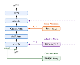
Cross-Attention for Text Conditioning
Text conditioning is the most common form of control in video generation. Given a text prompt (e.g., “A cat playing piano in a jazz club”), a pre-trained text encoder produces a sequence of contextual embeddings that guide the denoising process.
Definition 39 (Text Cross-Attention).
Let be the video token representations and be the text encoder output, where is the text sequence length and is the text embedding dimension. The text cross-attention computes (Cross ATTN QKV) where , , are learnable projection matrices. The queries come from the video tokens, while the keys and values come from the text tokens.
Proposition 22 (Cross-attention as soft dictionary lookup).
The cross-attention output for video token can be written as (Cross ATTN Lookup) which is a soft weighted average of the text value vectors . The weights form a probability distribution over text tokens, with higher weight on tokens whose keys are more aligned with the video query. This can be interpreted as a differentiable dictionary lookup: the video token “asks a question” (its query), and the text tokens “answer” according to their relevance (their key-value pairs).
Proof.
This follows directly from the definition of softmax attention. The weights and by the softmax normalisation, so the output is a convex combination of value vectors.
Dual Text Encoders
A number of generation systems employ two text encoders with complementary strengths: a language model (such as T5 or LLaMA) that provides rich semantic embeddings, and a contrastive model (such as CLIP) that provides embeddings aligned with visual features. This is a design choice rather than a universal one - CogVideoX, for instance, conditions on T5-XXL alone - but it is common enough, and instructive enough, to be worth setting out carefully.
Definition 40 (Dual Text Encoder Conditioning).
Given a text prompt , two encoders produce (DUAL ENC T5) where captures detailed linguistic semantics (entity relationships, attributes, spatial descriptions) and captures visual-semantic alignment (what the described scene “looks like”).
The two encodings are combined by either:
Concatenation: (after projection to a common dimension ).
Separate cross-attention: Two independent cross-attention layers, one attending to and another to , with outputs summed.
Pooled global conditioning: The CLIP [CLS] token embedding is used as a global conditioning signal via adaLN, while the T5 sequence is used for cross-attention.
Remark 40.
The rationale for dual encoders is that each captures different aspects of the text. T5, being an encoder-decoder language model, produces contextualised embeddings that capture complex linguistic structure: negation (“a cat not wearing a hat”), spatial relations (“to the left of”), and temporal sequencing (“first walks, then runs”). CLIP, trained with contrastive image-text pairs, produces embeddings that are well-aligned with visual concepts but less sensitive to linguistic nuance. By combining both, the model accesses complementary information streams.
Example 27 (Conditioning dimensions in practice).
In a model following the dual-encoder design of Stable Diffusion 3:
T5-XXL produces tokens of dimension .
CLIP-L/14 produces tokens of dimension .
Both are projected to before concatenation, giving text tokens.
With video tokens and per head, the cross-attention matrix has entries, much smaller than the entries of self-attention.
For contrast, CogVideoX [17] uses a single text encoder, T5-XXL, with no CLIP branch at all; its text tokens reach the network not through cross-attention but through the joint attention of Definition 30, with modality-specific normalisation as described in Example 26. The two systems therefore differ in both the number of encoders and the injection pathway, which is worth keeping straight when comparing published token budgets.
Concatenation Conditioning
For conditioning signals that have the same spatiotemporal structure as the video (reference images, masks, depth maps), the simplest injection pathway is channel-wise concatenation before patchification.
Definition 41 (Concatenation Conditioning).
Let be the noisy latent and be the conditioning tensor. The concatenation conditioning forms the augmented input (Concat COND) where denotes concatenation along the channel axis. The patchification layer is modified to accept input channels: .
Example 28 (Image-to-video via concatenation).
For image-to-video generation, the reference image is encoded by the video autoencoder's image encoder to obtain . This is replicated times along the temporal axis and concatenated with the noisy latent: (IMG TO Video Concat) doubling the input channels to . A binary mask indicating which frames are conditioned (typically only frame 0) is also provided, either as an additional channel or through the timestep embedding.
Remark 41.
Concatenation conditioning is the most flexible pathway because it preserves the full spatial structure of the conditioning signal. It is particularly effective for tasks requiring pixel-level alignment between the conditioning signal and the generated video, such as video inpainting, super-resolution, and depth-conditioned generation. The trade-off is that it increases the per-patch dimension (and hence the embedding matrix size) and requires the conditioning signal to be available at the same spatial resolution as the latent tensor.
Conditioning as Entropy Reduction
We now provide an information-theoretic perspective on conditioning, showing that each conditioning signal reduces the entropy of the generation distribution in a quantifiable way.
Theorem 5 (Conditioning as Entropy Reduction).
Let denote the clean latent video and a conditioning signal. Then (Entropy Reduction) with equality if and only if and are independent. The entropy reduction is exactly the mutual information: (Mutual INFO) For multiple conditioning signals , the chain rule gives (Chain RULE Entropy) where each term represents the additional information provided by each signal beyond what was already known.
Proof.
The inequality is a fundamental property of Shannon entropy (conditioning reduces entropy). The equality is the definition of mutual information. Non-negativity follows from the Gibbs inequality (or equivalently, from the non-negativity of KL divergence). The chain rule decomposition follows from the chain rule for mutual information: , applied recursively.
Insight.
Each conditioning pathway reduces a different type of uncertainty. The chain rule in (Chain RULE Entropy) reveals that conditioning signals have diminishing marginal returns if they are redundant. A detailed text description already constrains the scene layout and content, so a reference image provides less additional information than it would without the text. Conversely, if the text is vague (“a nice video”), the reference image provides much more information. This information-theoretic view explains why the effectiveness of each conditioning pathway depends on the specificity of the other signals, and suggests that the model should learn to dynamically allocate attention to the most informative conditioning source at each denoising step.
Proposition 23 (Gaussian entropy reduction bound).
If and are jointly Gaussian with , , and cross-covariance , then the entropy reduction is (Gaussian MI) where and are the marginal covariances. When the cross-covariance has rank (i.e., only modes of are correlated with ), the mutual information is bounded by , where measures the signal-to-noise ratio of the correlated modes.
Proof.
For jointly Gaussian variables, the conditional distribution is also Gaussian with covariance . The mutual information for Gaussian distributions is . The rank- bound follows from the fact that at most eigenvalues of the matrix inside the are non-zero, with each contributing at most to the sum, where .
Exercise 19.
Consider a video generation model with three conditioning signals: text (), reference image (), and camera trajectory (). Assume the following mutual information values (in nats): , , , , .
Compute the conditional mutual information , the additional information from the image given the text.
Compute .
Interpret the result: which conditioning signal provides more unique information beyond the text?
If the unconditional entropy is nats, what fraction of the uncertainty is resolved by all three signals? What does this imply about the remaining “creative freedom” of the model?
Exercise 20.
Consider a single cross-attention head with , video tokens, and text tokens.
Compute the size of the cross-attention matrix and compare it to the self-attention matrix for video tokens alone.
If the text encoder produces embeddings of dimension and the video model has dimension , compute the number of parameters in the and projection matrices.
Show that the cross-attention output for each video token lies in the convex hull of the text value vectors.
What happens when all text tokens produce identical key vectors? What does this imply about the text encoder's role?
Mixture-of-Experts for Video
Scaling a video diffusion model to billions of parameters improves quality, but the computational cost of each denoising step grows proportionally with the parameter count. For video, where each sample requires dozens of sequential denoising steps on a high-dimensional latent tensor, this cost quickly becomes prohibitive. Mixture-of-Experts (MoE) architectures address this tension by decoupling model capacity (total parameters) from per-token computation (FLOPs per forward pass). The idea is simple: replace the dense feed-forward network in each transformer block with a collection of expert sub-networks, and for each token, route it to only a small subset of experts. The total parameter count can be enormous (providing capacity to represent complex functions), while the per-token FLOPs remain manageable (because only a few experts are activated per token).
In this section, we formalise the MoE layer, analyse the routing mechanism, derive the load balancing loss, and discuss the intriguing phenomenon of expert specialisation by noise level in video diffusion models.
The MoE Layer
Definition 42 (Mixture-of-Experts Layer).
A Mixture-of-Experts layer with experts consists of:
A set of expert networks , where each expert is typically a feed-forward network (two linear layers with a non-linearity).
A gating network (router) that produces a score for each expert.
The output for input token is (MOE Output) where is the gating weight for expert and (or the sum is over only the selected experts in sparse MoE).
Remark 42.
In a dense MoE, all experts are evaluated for every token. This provides maximum expressiveness but no computational savings. In a sparse MoE, only a small subset of experts is evaluated per token, with the remaining experts receiving zero gate weight. Sparse MoE is the standard choice in practice because it achieves the capacity-compute decoupling that motivates the architecture.
Top- Routing
The most common routing strategy selects the top- experts for each token based on the gating scores.
Definition 43 (Top- Expert Routing).
Given an input token and a router weight matrix , compute the router logits (Router Logits) Select the indices of the top- logits: (TOPK Indices) and compute the gating weights via a restricted softmax: (TOPK GATE) The MoE output is then (MOE Sparse Output)
Proposition 24 (Computational savings of sparse MoE).
Let each expert be a two-layer FFN with hidden dimension , requiring parameters and FLOPs per token (accounting for both linear layers). A dense FFN with the same per-token cost has parameters. A sparse MoE layer with experts and top- routing has: (MOE Params) The capacity amplification factor is (MOE Amplification) which can be large (e.g., ) while the per-token FLOPs increase by only a factor of (plus the small routing overhead).
Proof.
The total parameter count sums the expert FFNs (each with parameters in the two linear layers) and the routing matrix (). The per-token FLOPs include expert evaluations ( for the two matrix multiplications in each FFN) plus the routing computation ( for the matrix-vector product ). The approximation in (MOE Amplification) drops the routing overhead, which is small when .
Example 29 (MoE in a video DiT).
Consider a video DiT with , , experts, and active experts per token.
Dense FFN: parameters per layer.
MoE layer: parameters per layer.
FLOPs per token: Dense: . MoE (): .
Capacity amplification: the layer holds the parameters of a dense FFN while costing the FLOPs per token, so parameters per unit of compute rise by .
For a 40-layer network where every other layer is MoE (20 MoE layers), this adds roughly B parameters beyond the dense baseline, while only doubling the FFN FLOPs in those layers.
Load Balancing
A well-known failure mode of MoE is expert collapse: the router learns to always send tokens to the same small subset of experts, leaving most experts unused. This wastes parameters and reduces the effective capacity of the model.
Definition 44 (Load Balancing Loss).
Given a batch of tokens , define the fraction of tokens routed to expert : (Expert Fraction) and the average routing probability for expert : (Expert PROB) where is the router logit for token and expert . The load balancing loss is (LOAD Balance LOSS) where is a balancing coefficient (typically ) and the factor ensures that the loss is regardless of the number of experts.
The constraints on these quantities will be used repeatedly, and are worth recording explicitly. Because top- routing selects distinct experts for each token, each indicator in (Expert Fraction) is or and each token contributes to exactly of the counters, so (Balance Constraints) In particular can never exceed : it is a fraction of tokens, not a count of selections.
Proposition 25 (Range of the load balancing loss).
Assume, as (Balance Constraints) guarantees, that with and that lies in the probability simplex. Assume further that and are similarly ordered, that is, for all (this last hypothesis is needed only for the lower bound). Then (Balance Range) a dynamic range of . The lower bound is attained by perfectly uniform routing, and for all ; the upper bound is attained by total collapse, in which a single expert receives every token () and absorbs all of the routing probability ().
Proof.
Lower bound. For similarly ordered sequences, Chebyshev's sum inequality gives , so and . Substituting , gives equality.
Upper bound. Using and , , so . Under total collapse the router assigns probability to for every token, so and (every token selects among its ), while the remaining selections land on experts with ; the sum is exactly and the bound is attained.
Caution.
The hypotheses in Proposition 25 are load-bearing. It is sometimes claimed that uniform routing minimises by Cauchy–Schwarz. It does not: Cauchy–Schwarz produces an upper bound on an inner product, and as a free bilinear form over the two constraint sets the sum is minimised at , by putting all of 's mass on an expert with . What rules that configuration out is not an inequality but the coupling: and are computed from the same router logits, so an expert with a larger average routing probability will ordinarily also receive a larger share of the top- selections. That is precisely the similarly-ordered hypothesis, and Chebyshev's sum inequality - not Cauchy–Schwarz - is the tool it feeds. Likewise, the maximum is and not : a collapsed router has , not , because top- routing cannot select the same expert times for one token.
Lemma 6 (Gradient of the load balancing loss).
The load balancing loss provides gradients only through the soft routing probabilities (which are differentiable with respect to the router weights), not through the hard token assignments (which involve a non-differentiable top- selection and are treated as constants). The gradient with respect to the router logit is (Balance GRAD) where . The parenthesised factor in the first form is the amount by which the utilisation of expert exceeds the utilisation of the experts this token is currently inclined to choose, averaged under . The gradient is therefore positive - pushing the logit, and hence the routing probability, down - exactly when expert is over-utilised relative to that token-specific reference, and negative when it is under-utilised.
Proof.
Write with and treat as constant. The softmax Jacobian is , which includes the off-diagonal terms . Hence which is the first form; factoring out the term of the sum gives the second. Retaining the off-diagonal terms matters: they are what makes the gradient sum to zero over for each token, , as it must, since adding a constant to all logits of a token leaves - and therefore the loss - unchanged.
Expert Specialisation by Noise Level
A remarkable empirical observation in MoE-based video diffusion models is that different experts tend to specialise for different noise levels (timesteps). At high noise (), certain experts dominate, handling coarse, global structure prediction. At low noise (), different experts activate, handling fine detail refinement.
Definition 45 (Timestep-Dependent Expert Utilisation).
For a given timestep , define the expert utilisation profile as the vector (Expert Utilisation) where is the expected fraction of tokens routed to expert when the input is at noise level . By (Balance Constraints) each lies in and (Utilisation SUM) So is not a probability vector unless ; it is a vector of marginal selection frequencies that sum to the number of experts each token activates. Dividing by makes it one, and is the more convenient object when comparing utilisation profiles across configurations with different .
Proposition 26 (Noise-level specialisation as mode separation).
Consider a simplified model where the denoising task at noise level requires one of distinct “modes” of computation (e.g., coarse structure prediction, mid-level feature generation, fine detail refinement). If and the router is trained to minimise the denoising loss with the load balancing regulariser, the equilibrium routing satisfies: (Specialisation) where maps timestep to its associated mode and is the number of experts assigned to mode . That is, experts naturally cluster into groups, with each group handling a specific range of noise levels.
Proof sketch.
The denoising objective at different noise levels requires different types of transformations: at high noise, the gradients favour low-frequency prediction (global structure), while at low noise, they favour high-frequency prediction (fine details). If the expert FFNs have limited capacity, it is more efficient for each expert to specialise in one type of transformation than to be a generalist. The load balancing loss prevents all tokens from collapsing to the same experts but does not prevent noise-level clustering. A more rigorous treatment requires analysing the optimisation dynamics of the router in the presence of timestep-varying input distributions, which we leave as an open question.
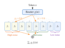
Capacity Factor and Auxiliary Losses
In distributed training, MoE layers introduce a unique challenge: tokens must be dispatched to the devices hosting each expert, and imbalanced routing can cause memory overflow on some devices while leaving others idle. The capacity factor controls how many tokens each expert can process.
Definition 46 (Capacity Factor).
Given a batch of tokens distributed across experts with top- routing, the expert buffer size is (Capacity Factor) where is the capacity factor. Each expert processes at most tokens; tokens that would exceed this capacity are dropped (their expert computation is skipped, and the token passes through a residual connection instead). A capacity factor of means each expert receives exactly the average number of tokens under perfect balance; provides a buffer for imbalance.
Caution.
Setting the capacity factor too low causes token dropping, which degrades generation quality because some tokens miss their expert computation entirely. Setting it too high wastes memory and compute on empty buffer slots. For video diffusion, where every token contributes to the final frame quality, aggressive token dropping (CF ) can cause visible artefacts in the generated video, particularly in regions with unusual motion patterns that trigger non-uniform routing.
Definition 47 (Z-Loss Regulariser).
An additional auxiliary loss that prevents router logits from growing too large (which would cause numerical instability in the softmax) is the Z-loss: (Z LOSS) where is a small coefficient (typically ). This loss penalises large logsumexp values, encouraging the router logits to remain moderate in magnitude.
Proposition 27 (Total training objective with MoE).
The total training objective for a video diffusion model with MoE layers is (MOE Total LOSS) where is the standard denoising objective (e.g., -prediction MSE or flow matching loss) and the sum runs over all MoE layers . The auxiliary losses and are summed over layers (not averaged) to ensure that each layer receives adequate regularisation.
Remark 43.
Not every layer in a video DiT needs to be an MoE layer. A common design pattern is to use MoE layers at every other position (or every fourth position), with standard dense FFN layers in between. This reduces the routing overhead and the total parameter count while still providing substantial capacity amplification. The accounting is worth doing carefully, because it is easy to double-count. Take a 40-layer network with MoE at every other layer (, ), and measure everything in units of one dense FFN layer. The network has 20 dense FFN layers and 20 MoE layers, so:
FFN parameters: dense-FFN-equivalents (each MoE layer holds expert FFNs).
FFN FLOPs per token: dense-FFN-equivalents (each MoE layer evaluates experts). The dense layers are counted once, not twice.
Amplification: more FFN parameters per unit of FFN compute than the fully dense 40-layer baseline, which sits at .
Equivalently, relative to the dense baseline the design buys the FFN parameters for the FFN FLOPs. The per-layer amplification of applies only to the MoE layers themselves; diluting them with dense layers necessarily brings the whole-network figure below it.
Exercise 21.
Consider a video DiT with the following specifications: layers, , , and attention heads. Every even-numbered layer uses MoE with experts and top- routing.
Compute the total parameter count for the attention layers (all 32 layers are identical).
Compute the total parameter count for the FFN layers, distinguishing between dense (16 layers) and MoE (16 layers).
Compute the total model parameters and compare to a fully dense model of the same depth and width.
Estimate the per-token FLOPs for a forward pass and compare to the dense baseline.
If perfect load balancing is achieved, how many tokens does each expert process in a batch of tokens?
Exercise 22.
Consider a simplified MoE with experts and routing. Suppose the denoising task at noise level is characterised by a “task vector” such that the optimal FFN transformation at that noise level is approximately .
If the experts are linear functions , show that the optimal routing assigns each timestep to the expert whose weight matrix is closest to in Frobenius norm.
Suppose varies smoothly with . Argue that the optimal expert assignment partitions the interval into (at most) contiguous segments.
Relate this to the empirical observation that experts specialise by noise level.
Exercise 23.
Let with and let lie in the probability simplex, as in (Balance Constraints).
Suppose and are similarly ordered. Prove that using Chebyshev's sum inequality, and deduce .
Show that equality in (a) holds whenever either of the two vectors is constant across experts. Conclude that the minimiser is not unique: exhibit a non-uniform that also attains .
Drop the similarly-ordered hypothesis. Construct explicit satisfying the constraints for which , and explain why such a configuration cannot arise from a top- router that computes and from the same logits.
Using only and , prove , so . Identify the routing configuration that attains it, and verify that the dynamic range of the loss is .
Is a convex function of the pair ? Compute the Hessian of the scalar function to justify your answer, and then state what is true of when one of the two arguments is held fixed. Does the minimiser you found in (b) contradict the phrase “unique minimiser”?
From Architecture to Objective
sec:vdiff:dit,sec:vdiff:factored-attn,sec:vdiff:3d-pe,sec:vdiff:conditioning,sec:vdiff:moe have specified a network. Its design reduces to five decisions, each of which is a purchase made against a fixed compute budget:
Tokenisation (Spatiotemporal Patchification): spatiotemporal patches of size turn the latent tensor into tokens. The patch size is the cheapest available lever on cost, and the bluntest one on quality.
Conditioning on the noise level (The DiT Block with Adaptive Layer Normalisation): adaLN supplies a global, -dependent per-channel gain and offset, and the adaLN-Zero gates make every block the identity at initialisation. As Proposition 13 makes precise, this buys trainability, not representational power.
The attention pattern (Factored Attention for Video): full spatiotemporal attention is and, at realistic token counts, simply unaffordable. Factorisation, alternating blocks and 3D windows each restrict the attention graph in a different way, with provable savings and empirical - not provable - quality costs.
Position (3D Positional Encoding): 3D RoPE makes the attention logit a function of the displacement alone, which is what allows a model trained at one resolution and duration to be run at another.
Capacity (Mixture-of-Experts for Video): mixture-of-experts decouples parameter count from per-token FLOPs, at the price of a routing problem that must be regularised into balance.
What this network is for has so far been left implicit. We have assumed only that it consumes a noised latent and a timestep and emits a prediction, without committing to what that prediction is, how the noise levels are distributed, or how the trained model is run at inference. Those are the subjects of the sections that follow, and each of them turns out to require modification for video rather than inheritance from image diffusion.
Noise Schedules for Video takes up the noise schedule. A schedule tuned for a image is systematically too easy for a video latent that is an order of magnitude larger, because at equal per-element signal-to-noise ratio a higher-dimensional observation carries more evidence about the clean sample; the remedy is a shift of the log-SNR curve by the ratio of dimensionalities, tempered by the fact that temporal correlation makes the effective dimensionality of a video smaller than its nominal one. Flow Matching for Video replaces the diffusion SDE with flow matching along straight optimal-transport paths, and shows why straightness is what makes few-step sampling viable; it also covers rectified flow, the v-prediction parameterisation, and the stochastic-interpolant framework that contains both flow matching and diffusion as special cases. Sampling Acceleration attacks inference cost along three orthogonal axes - fewer steps via deterministic solvers and consistency distillation, cheaper steps via temporal feature caching, and better solvers - and shows how the savings compound. Finally, Training at Scale describes how such models are actually trained: multi-stage curricula that begin with images and end at high resolution, mixed image-video batches, data curation pipelines that discard the great majority of the raw corpus, and the compute budgets these recipes imply.
Only after those pieces are in place does the question of control - guidance, image conditioning, camera trajectories, personalisation - become well posed, and that is where the chapter turns next.
Noise Schedules for Video
The noise schedule is the heartbeat of every diffusion model. It determines how quickly the data signal is destroyed during the forward process and, consequently, how the denoiser must allocate its capacity across timesteps. For images, the design of noise schedules is well-studied: the cosine schedule of Nichol and Dhariwal, the linear schedule of Ho et al., and the learned schedules of Kingma et al. all provide effective ways to spread the denoising task across a manageable number of steps.
For video, however, the situation is fundamentally different. A video tensor contains far more elements than an image tensor , and those elements are highly correlated along the temporal axis. Both of these facts have profound consequences for the signal-to-noise ratio (SNR) at each timestep, and ignoring them leads to degenerate training behaviour. In this section, we develop the theory of noise schedules for video, starting from the observation that standard image schedules fail when applied naively to video data.
Why Image Schedules Fail for Video
Recall the forward process of a continuous-time diffusion model. Given a clean data sample , the noisy version at time is (Forward ZT) where and define the schedule. The signal-to-noise ratio at time is (SNR DEF) For images, a typical cosine schedule produces (nearly clean) and (nearly pure noise), with a smooth transition between the two extremes.
The problem arises when we consider what the denoiser “sees” at each timestep. At intermediate , the denoiser receives a mixture of signal and noise. For the denoiser to learn effectively, it must encounter timesteps where the task is neither trivially easy (pure signal) nor impossibly hard (pure noise). The range of “useful” timesteps depends on the dimensionality of the data.
Insight.
Redundancy, not raw dimensionality, shifts the effective noise level. It is tempting to argue that a larger tensor is easier to denoise simply because it has more elements, but that argument is wrong as stated. If the coordinates of were statistically independent, the denoising problem would factorise into independent scalar problems and the per-coordinate difficulty would not depend on at all. What makes visual data different is that its coordinates are massively redundant: neighbouring pixels, and neighbouring frames, are near-copies of one another. The denoiser can therefore average many noisy observations of what is essentially a single underlying quantity - the shared signal adds coherently while the independent noise partially cancels - so a group of nearly identical coordinates behaves like one coordinate observed at times the SNR. Because redundancy grows as we add pixels and frames, timesteps that are “informative” for an image become “too easy” for a video, and the image schedule wastes training capacity on them. The quantity that controls the correct shift is thus a redundancy factor, made precise in Theorem 6.
To make this precise, consider the log-SNR, defined as . For an image diffusion model at resolution with latent channels, the effective dimensionality is . For a video with latent frames, it is . The ratio can be large (e.g., to for typical video models).
Example 30 (SNR mismatch between image and video).
Consider a cosine schedule designed for latent images (, the latent of a image under an spatial autoencoder). For a video with latent frames at the same spatial resolution, . Both models are trained at the same nominal per-element SNR, since is a per-element quantity and does not depend on at all. What differs is how much of that dimensionality is redundant: consecutive latent frames of a natural clip are strongly correlated, so the video denoiser can average along the temporal axis and recovers the shared content at an effective SNR several times larger than the nominal one. Timesteps that sit inside the image model's informative band therefore sit above the video model's, and the image schedule spends capacity on timesteps the video model finds trivial. Counting dimensions alone (Definition 48) would prescribe a downward log-SNR shift of nats; Theorem 6 shows this is an upper bound on the shift that is actually warranted, and quantifies the gap.
The SNR Shift Principle
The solution, first proposed in Imagen Video [5] and analysed in detail by Chen [23], is to shift the noise schedule so that the SNR at each timestep is adjusted for the data dimensionality.
Definition 48 (Shifted SNR Schedule for Video).
Let be a reference noise schedule designed for data of dimensionality (e.g., a latent image). The shifted SNR schedule for video data of dimensionality is defined by (Shifted SNR) where the shift factor accounts for the increased dimensionality: (Shift Factor) In log-SNR space, the shift becomes an additive offset: (Logsnr Shift)
The shift factor when , which decreases the SNR at every timestep. Equivalently, the log-SNR curve is shifted downward, moving the “informative” range of timesteps earlier. This is the rule used in practice, and for spatial upscaling it is well supported empirically: natural images are redundant at every scale, so quadrupling the pixel count does buy the denoiser close to a fourfold gain in effective SNR.
Remark 44.
It is worth being precise about what (Shift Factor) assumes. Adding coordinates makes denoising easier only to the extent that the added coordinates are copies of information already present. If the frames of a clip were exact copies of one another, the denoiser could average them and gain a factor in SNR, and dividing the SNR by would restore the original difficulty - which is exactly when only the frame count changes. If instead the frames were statistically independent, averaging would buy nothing and no shift would be warranted. The dimension-counting rule therefore silently assumes the maximum possible redundancy along every axis it counts. Temporal Redundancy and the Shift It Justifies replaces that assumption with a measurable quantity.
Temporal Redundancy and the Shift It Justifies
The shift principle of Definition 48 counts every dimension of the video tensor as if it were a fresh copy of the signal. As Remark 44 observed, that is the perfectly-redundant limit. We now make the redundancy of a video measurable and derive the shift it actually justifies.
The right notion is a spectral one. Write for the ambient dimension of the clean latent and for its covariance. If the coordinates were uncorrelated with equal variances, nothing could be averaged; if they were all copies of a single scalar, everything could be. The participation ratio interpolates between these two extremes, and its reciprocal (normalised by ) is exactly the factor by which the SNR must be lowered.
Theorem 6 (Redundancy-Matched Noise Schedule).
Let the clean latent be zero-mean Gaussian with covariance , normalised so that (unit average per-coordinate variance), and let as in (Forward ZT). Measure the difficulty of the denoising task at by the normalised denoising MMSE (Nmmse) where are the eigenvalues of (so ). Define the redundancy factor and the effective dimension (EFF DIM) Then:
(Range.) , with if and only if is a multiple of the identity (no redundancy, ), and if and only if has rank one (total redundancy, ).
(Difficulty matching.) as . Consequently the video and reference difficulty profiles agree in the high-noise regime if and only if , that is, if and only if the two log-SNR schedules differ by the constant offset (Optimal Logsnr)
(Exactness.) If the spectrum of is an -fold replication of that of - that is, and the eigenvalues are together with zeros - then for every , so (Optimal Logsnr) matches the two difficulty profiles at every timestep, not merely at high noise.
(Separable video covariance.) Suppose , where is the temporal correlation matrix of the centred frames () and is the per-frame spatial covariance on coordinates. Then the redundancy factor factorises, , with the temporal redundancy factor (Temporal Redundancy) If the reference schedule was designed for a single frame with the same spatial statistics, then and the video-specific shift is exactly (Video Shift)
Writing for the effective number of independent frames, the special cases are:
Independent frames (): , , and no temporal shift is warranted. The video denoising problem factorises into copies of the image problem, so the image schedule is already correct.
Identical frames ( for all ): , , and the shift is - exactly the dimension-counting shift of Definition 48.
Exponentially decaying autocorrelation (): when , and when .
Note that (a) and (b) bracket the truth from the two sides: real video sits strictly between them, so the correct shift is smaller in magnitude than the dimension-counting shift, by nats.
Proof.
(i) Since , Cauchy–Schwarz gives , hence with equality iff all are equal. Non-negativity of the eigenvalues gives , hence with equality iff exactly one eigenvalue is non-zero.
(ii) For jointly Gaussian the posterior has covariance , whose eigenvalues are with ; summing and dividing by gives (Nmmse). (Only the second-order statistics of enter; for non-Gaussian data (Nmmse) is the MMSE of the best linear estimator, hence an upper bound on the true MMSE.) Expanding , (Nmmse Expansion) so is precisely the initial slope of the difficulty curve. Two such curves agree to first order at exactly when the products coincide, which is (Optimal Logsnr) after taking logarithms.
(iii) Under the replication hypothesis, (Replication) the zero eigenvalues contributing nothing. Its redundancy factor is , so the required offset is .
(iv) The eigenvalues of a Kronecker product are the pairwise products of the eigenvalues of the factors, so both and factorise, and therefore so does . For the temporal factor, because , and , giving (Temporal Redundancy); the bounds are (i) applied to .
Special cases. For (a), and , so . For (b), is the all-ones matrix and , so . For (c), put and collect terms by the lag : (RF Exponential) As with fixed this tends to , which is for large ; as with fixed, and .
Remark 45 (What the theorem does and does not say).
Three caveats are worth stating plainly. First, “optimal” here means only difficulty-matched: the schedule that reproduces the reference model's normalised-MMSE profile. That is a design criterion, not a theorem about sample quality. Second, the argument uses only second-order statistics. Motion, occlusion and object permanence are not second-order phenomena, so captures the part of temporal redundancy that linear averaging can exploit and nothing more. Third, must be computed on centred latents; a non-zero mean makes tend to a positive constant and inflates arbitrarily.
Remark 46.
In practice is estimated directly from a batch of encoded training videos: centre the latents, compute the sample autocorrelation along the frame axis, and evaluate (Temporal Redundancy). For an order-of-magnitude figure, Proposition 2 puts the pixel-domain decorrelation timescale of general-motion footage at roughly to frames, and a temporal autoencoder divides that by four, leaving to latent frames. By case (c) this gives to , i.e. to , and hence a temporal shift of to nats. The dimension-counting rule would instead prescribe nats at and nats at , so it over-shifts by one to three nats - enough to matter, but far from the whole schedule. The practical recipe is therefore: apply the full Definition 48 shift on the spatial axes, and a measured on the temporal axis.
Resolution-Adapted SNR
Modern video generation systems produce outputs at multiple resolutions, either through cascaded super-resolution or through direct generation at variable resolution with packing strategies. The noise schedule should adapt to the target resolution.
Proposition 28 (Resolution-Adapted SNR).
Let be the dimensionality of the video latent at the target resolution and the reference dimensionality (e.g., a latent image). The resolution-adapted log-SNR schedule is (Resolution Adapted) Equivalently, if the reference schedule uses signal and noise coefficients , the adapted schedule uses (Adapted Coefficients) where the constant of proportionality at each is fixed by whatever normalisation the model assumes; for a variance-preserving schedule one rescales the pair so that , which is what (Shifted Alpha Sigma) does. (Only the ratio is determined by the log-SNR shift.)
Proof.
This follows directly from Definition 48 by substituting into (Logsnr Shift). Expressing in terms of : the adapted SNR is , which fixes the ratio and hence the pair up to a common scale.
Remark 47.
Proposition 28 is stated for the full dimensionality because that is what implementations do. By Theorem 6 it is well justified for the spatial factor and is an upper bound on the shift for the temporal factor: replacing by the measured redundancy in gives the redundancy-matched version.
Example 31 (Schedule shifts for common configurations).
tab:vdiff:schedule-shifts shows the log-SNR shift for several common video generation configurations relative to a reference latent image.
tableLog-SNR shifts for various video latent configurations.
Negative values indicate that the schedule must be shifted toward
higher noise.
Configuration Image (, ref) 1 4,096 Image () 1 16,384 Short video (17 lat. frames) 17 69,632 Medium video (33 lat. frames) 33 304,128 Long video (65 lat. frames) 65 1,064,960
Remark 48.
Chen [23] showed that applying this resolution-adapted shift is essential for training diffusion models at high resolution. Without the shift, the model spends most of its capacity on timesteps where the task is trivially easy (the signal overwhelms the noise in high-dimensional space), leading to poor sample quality. The same principle applies with even greater force to video, where the dimensionality increase is an order of magnitude beyond what is encountered in high-resolution image generation.
Visualising the SNR Shift
The following figure illustrates how the log-SNR curve shifts downward as the data dimensionality increases from a single image to increasingly long video sequences.
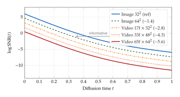
Implementation: Shifted Cosine Schedule
In practice, the shifted schedule is implemented by modifying the standard cosine schedule. The reference cosine schedule defines (Cosine REF) so that . The shifted video schedule is obtained by applying the log-SNR offset: (Shifted Cosine) To express this in terms of satisfying (variance-preserving), we define (Shifted Alpha Sigma)
Caution.
When the shift factor is very small (long, high-resolution videos), the SNR at may no longer be large enough to ensure that the noisy latent at is close to the clean data . In this regime, it is common to clamp the SNR at to a minimum value (e.g., ) and at to a maximum noise level (e.g., ). The clamping ensures that the boundary conditions of the diffusion process remain well-defined.
Exercise 24 (Computing the shift factor).
A video diffusion model generates 65 latent frames at spatial resolution with latent channels. The reference schedule was designed for latent images.
Compute and .
Compute the log-SNR shift .
If the reference schedule has (unit SNR at the midpoint), what is under the dimension-counting rule?
The latents have temporal autocorrelation with latent frames. Using (RF Exponential), compute the temporal redundancy factor and the effective frame count .
Hence compute the redundancy-matched shift of Theorem 6, where is the per-frame latent dimension, and say by how many nats it differs from the answer to (b). Which of the two schedules puts more noise into the middle of the trajectory?
Answers for checking: (a) , ; (b) ; (d) , ; (e) , i.e. nats less noise than (b).
Exercise 25 (Deriving the temporal redundancy factor).
Prove case (c) of Theorem 6. For , write and show first that collecting the double sum by the lag gives (Double SUM EXP)
Evaluate the sum in closed form and verify (RF Exponential). Hint: use and .
Deduce the limit as , and as with fixed.
Explain in one sentence why the square of appears here, whereas a naive “count the correlated frames” argument would use itself. Hint: came from , a sum of squared eigenvalues.
Flow Matching for Video
The diffusion models we have discussed so far are formulated as stochastic processes: the forward process adds noise through a stochastic differential equation (SDE), and the reverse process removes it by running the SDE backwards in time. An alternative formulation, flow matching, replaces the stochastic process with a deterministic ordinary differential equation (ODE) that transports samples from a noise distribution to the data distribution. This ODE-based viewpoint offers several advantages: simpler training objectives, straighter sampling trajectories (enabling fewer integration steps), and a natural connection to optimal transport theory.
Flow matching has become the dominant training paradigm for recent video diffusion models: Movie Gen [32] and Stable Diffusion 3 [24] are trained with an explicit flow matching objective on linear paths, and several video systems have followed. The picture is not uniform, however, and it is worth being accurate about it. CogVideoX [17] uses the -prediction parameterisation of a variance-preserving diffusion, which is closely related to but not identical with flow matching (Proposition 30); Stable Video Diffusion [8] is trained in the EDM framework with a preconditioned denoiser and a log-normal noise distribution, not with flow matching at all. In this section we develop the mathematical foundations of flow matching for video, building on the framework of Lipman et al. [25] and Liu et al. [26].
From Diffusion to Flow
Recall the forward process of a diffusion model: , where . This can be viewed as defining a probability path that interpolates between the data distribution and the noise distribution .
There exists a time-dependent velocity field such that the probability path is the pushforward of along the flow induced by . Formally, satisfies the continuity equation: (Continuity) The key insight of flow matching is that we can directly learn without ever working with the SDE formulation. Instead of training a score function and converting it to a velocity field, we train a neural network to predict the velocity field directly.
Key Idea.
Flow matching simplifies training. In the DDPM framework, the model predicts noise , and the loss involves the score function of the marginal distribution , which is intractable for complex data. Flow matching avoids this by conditioning on the sampled endpoints and learning the conditional velocity field , which has a simple closed form. This conditional formulation gives the same marginal velocity field in expectation, but each individual training target is a deterministic function of .
The Video Flow Matching Objective
We now formalise the flow matching framework for video generation. Let be a clean latent video and be pure noise.
Definition 49 (Video Flow Matching Objective).
The video flow matching (VFM) objective trains a velocity network by minimising (VFM LOSS) where is the interpolated sample at time and is the conditional velocity field defined by the chosen interpolation path. Throughout, denotes the data endpoint (at time ) and the noise endpoint (at time ); see Remark 49.
The definition is general; it applies to any choice of interpolation between and . The most common choice, and the one that connects to optimal transport theory, is the linear (or optimal transport) path.
Definition 50 (Optimal Transport Path).
The optimal transport (OT) path defines the interpolation (OT Interp) with the associated conditional velocity field (OT Velocity) At the path sits on the clean data sample and at on the noise sample , so the subscript of is always the time index and never a separate label.
Remark 49 (Time convention, stated once and used throughout).
Every result in this chapter uses one convention:
at ; at ; is the state at time .
Under the OT path convention of Definition 50, the VFM loss becomes particularly simple: (VFM OT LOSS) The training target is simply the displacement from data to noise, a fixed vector for each training pair ; sampling integrates the same field in the opposite direction.
Why OT Paths Are Preferred
The OT path is not the only possible interpolation. One could also use the variance-preserving (VP) path defined by , which corresponds to the DDPM forward process with the cosine schedule of (Cosine REF). However, the OT path has a crucial geometric advantage.
Proposition 29 (Straighter Trajectories).
Among all interpolation paths with and boundary conditions , the linear (OT) path is the unique minimiser of the trajectory curvature (Curvature) for every sample pair with linearly independent, and it attains .
Proof.
For the linear path, , so (constant) and ; hence , which is the minimum since always. Conversely, if and are linearly independent then vanishes for a.e. only if , i.e. only if and are affine, and the boundary conditions then force , .
Insight.
Straight paths enable few-step sampling. The practical significance of Proposition 29 is enormous. When the learned velocity field generates approximately straight trajectories, the ODE can be solved with very few Euler steps (as few as 1 to 4 steps) without significant discretisation error. Curved trajectories, by contrast, require many steps to track accurately. For video generation, where each step involves a full forward pass through a large transformer, reducing the step count from 50 to 4 translates to a speedup.
Rectified Flow and Iterative Straightening
While the OT path is straight for individual sample pairs, the marginal velocity field may still generate curved trajectories, because different data points paired with different noise points create crossing paths in the shared space. Rectified flow [26] addresses this by iteratively straightening the learned flow.
Theorem 7 (Rectified Flow for Video).
Let be any coupling of with with (in practice the independent coupling), and define the reflow procedure: at round ,
let be the marginal velocity field of the linear interpolation of the current coupling;
sample and integrate backwards from to to obtain ;
take as the coupling for round .
Assume the velocity field is exact (no approximation error) and the ODE is solved exactly. Then, writing and defining the straightness deficit (Straightness) the following hold.
Marginals are preserved and every convex transport cost is non-increasing: for all , and for every convex , . In particular .
The flow straightens at rate : , hence . A coupling with has trajectories that are exactly straight, so a single Euler step integrates it without error.
Straight does not mean optimal. The fixed points of reflow are exactly the couplings with . Such a coupling is deterministic and its trajectories do not cross, but in dimension these properties do not characterise the optimal transport coupling, and rectified flow is not guaranteed to converge to the Monge map. Only for does non-crossing force the monotone rearrangement, which is the optimal map for every convex cost.
Proof.
(a) Marginal preservation is the defining property of the marginal velocity field: the ODE driven by transports the law of to the law of , and by construction has the same law as for every . For the cost, write the new displacement as an integral of the velocity along the trajectory, , and apply Jensen's inequality twice: once to move inside the time integral (convexity in the integrand), and once to move inside the conditional expectation defining . Since , taking expectations gives , because the conditional interpolation has constant velocity. This is the convex-transport-cost reduction theorem of Liu et al. [26].
(b) Take . Because is a conditional expectation, the variance decomposition gives, for each , . Integrating over and using (Jensen again) yields . Summing over and using gives , and the minimum of non-negative terms with that sum is at most .
(c) If then is -measurable for a.e. , so the interpolation paths through any point at time all carry the same velocity: the coupling is deterministic with non-crossing straight paths, and reflow leaves it unchanged. The converse fails: in one can construct straight non-crossing couplings that are not optimal for the quadratic cost, and Liu et al. state explicitly that rectification is not guaranteed to yield the optimal coupling - what it monotonically improves is the transport cost, not the optimality gap. In , a non-crossing coupling is the monotone rearrangement, which is the unique optimal coupling for every convex cost; this is the only dimension in which “straight and non-crossing” and “optimal” coincide.
Caution.
Parts (a) and (b) are statements about the exact marginal velocity field. In practice is replaced by a learned network and the ODE by a discretisation, and both errors accumulate across reflow rounds - which is the practical reason (independent of the theory) that no one runs more than one or two rounds.
Remark 50.
In practice, one or two reflow iterations suffice to achieve nearly straight trajectories - which, by Theorem 7(b), is all that few-step sampling requires; it is not necessary (and not true) that the coupling becomes optimal. The Stable Diffusion 3 model [24] uses a single reflow iteration combined with distillation to enable high-quality generation in 4 to 8 steps. For video models, reflow is more expensive (each iteration requires generating a full dataset of video samples), but even without reflow, the OT path provides much straighter trajectories than the VP path used in DDPM.
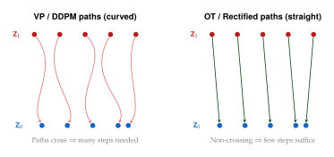
v-Prediction Parameterisation
The flow matching velocity is closely related to the classical parameterisations used in diffusion models. We now make this connection precise.
Under the linear interpolation (where is data at and is noise at ), the velocity field can be decomposed in terms of either the noise prediction or the data prediction .
Proposition 30 (Equivalence of Parameterisations).
Given the OT interpolation , the following parameterisations are equivalent for :
Velocity (v-prediction): .
Data prediction (-prediction): predicts . The velocity is recovered as (V FROM X0)
Noise prediction (-prediction): predicts (the noise). The velocity is recovered as (V FROM EPS)
The conversions between parameterisations are: (X0 FROM V)
Proof.
From and we get the two identities (DATA Noise FROM ZT) Solving the first for with replaced by its prediction gives (V FROM X0), and solving the second for with replaced by gives (V FROM EPS). Rearranging the same two identities gives eq:vdiff:x0-from-v,eq:vdiff:eps-from-v.
Remark 51.
The v-prediction parameterisation has a practical advantage: it is numerically stable across all timesteps . The division by in (V FROM X0) and by in (V FROM EPS) is exactly where the other two parameterisations degrade. -prediction is ill-conditioned near (where is nearly pure noise and predicting is very hard), and -prediction is ill-conditioned near (where is nearly clean and the noise must be inferred from a vanishing residual). The velocity has bounded magnitude at all timesteps, avoiding both instabilities.
Training Algorithm
We now present the complete training procedure for video flow matching.
Algorithm 4 (Video Flow Matching Training).
Input: Video dataset , velocity network , learning rate , noise schedule shift (from Noise Schedules for Video), classifier-free guidance dropout probability . Output: Trained velocity network .
For each training iteration: enumerate[(a)]
Sample a mini-batch of videos from .
Encode to latent space: for each .
Sample timesteps , adjusted according to the shifted noise schedule.
Sample noise: .
Compute interpolated samples: .
Compute target velocities: .
With probability , replace the text conditioning with the null embedding (for classifier-free guidance).
Compute the loss: (VFM Batch LOSS) where is a timestep-dependent weighting function and is the conditioning signal (text embedding, reference image, etc.).
Update parameters: . enumerate
Remark 52.
The weighting function in (VFM Batch LOSS) controls the relative importance of different timesteps during training. Common choices include:
Uniform: . Each timestep contributes equally to the loss.
SNR-weighted: . Emphasises timesteps where signal and noise are balanced.
Min-SNR: with . Clips the weight at high SNR to prevent easy timesteps from dominating.
Logit-normal: Sample from a logit-normal distribution rather than uniform, concentrating samples near where the denoising task is most informative. This is the approach used by Stable Diffusion 3 [24].
Sampling Algorithm
Given a trained velocity network , generating a video requires solving the ODE (FLOW ODE) backwards in time, from the noise endpoint down to the data endpoint (Remark 49). The simplest approach is the Euler method, which for a backward integration subtracts times the velocity at each step.
Algorithm 5 (Video Flow Matching Sampling (Euler ODE)).
Input: Trained velocity network , conditioning signal , number of steps , classifier-free guidance scale . Output: Generated latent video .
Sample initial noise: , .
Set step size: .
For : enumerate[(a)]
Set .
Compute the unconditional velocity: .
Compute the conditional velocity: .
Apply classifier-free guidance: (CFG Velocity)
Backward Euler step: . enumerate
Decode: .
Return .
Remark 53.
While the Euler method is simple, higher-order ODE solvers can improve sample quality at the same number of function evaluations. Common choices for video generation include:
Midpoint method (2nd order): evaluate at the midpoint and use this velocity for the full step. Requires 2 function evaluations per step but achieves 2nd-order accuracy.
Heun's method (2nd order): take a predictor Euler step, evaluate at the predicted point, then average the two velocities. Also 2 evaluations per step.
DPM-Solver (2nd/3rd order): a solver specifically designed for diffusion ODEs that exploits the structure of the noise schedule to achieve higher accuracy with fewer evaluations.
For well-trained flow matching models with nearly straight trajectories, even the simple Euler method produces high-quality results in 20 to 50 steps. With rectified flow or distillation (Sampling Acceleration), as few as 4 to 8 steps may suffice.
Stochastic Interpolants Perspective
The flow matching framework can be generalised through the stochastic interpolants framework of Albergo et al. [66], which provides a unified view encompassing both deterministic flows and stochastic diffusion processes.
Definition 51 (Stochastic Interpolant).
A stochastic interpolant is a process of the form (Stochastic Interpolant) where are smooth functions satisfying the boundary conditions: (Interpolant BC) (We write rather than to avoid a collision: are already the signal and noise coefficients of (Forward ZT), and is the Min-SNR clipping constant of Remark 52. Note that is the data coefficient, so plays the role of and that of .)
Setting recovers the deterministic flow matching framework. Setting adds stochasticity to the interpolation, which can improve mode coverage at the cost of requiring more sampling steps. The OT flow matching framework corresponds to , , .
Example 32 (Common interpolation schemes).
tab:vdiff:interpolation-schemes summarises several interpolation schemes used in practice.
tableInterpolation schemes and their properties. Here
sits at and
at , so is the data
(signal) coefficient and the noise coefficient;
is the usual DDPM cumulative product.
Scheme Used by OT / Linear SD3, Movie Gen VP (cosine) Imagen Video VP (DDPM) DDPM Stochastic OT Research
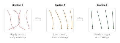
Exercise 26 (Flow matching derivations).
Starting from the VP interpolation , derive the conditional velocity field . Show that it depends on (unlike the OT case where is constant), and check that it can be written as .
Verify that the OT flow matching loss and the DDPM -prediction loss have the same minimiser (up to reparameterisation), using Proposition 30.
For a trained flow matching model with velocity field , derive the formula for the log-likelihood of a generated sample. Start from the instantaneous change of variables formula and integrate along the trajectory to obtain , where . Note the sign: the divergence term enters with a here only because time runs from the noise endpoint down to the data endpoint .
Exercise 27 (Euler discretisation error, and why the bound is not the reason few-step sampling works).
Consider the ODE on with a velocity field that is -Lipschitz in its first argument, for all . Let be the exact solution and let bound the second derivative of the solution (not of ).
Show that the explicit Euler method with uniform steps of size has global error bounded by (Euler Bound) Hint: the local truncation error over one step is at most by Taylor's theorem; propagate it with the discrete Grönwall inequality and use .
For a perfectly rectified flow the exact trajectory is a straight line traversed at constant speed. Show that , so (Euler Bound) gives zero error and a single Euler step is exact.
Now evaluate (Euler Bound) for a realistic video model. Take , and . Show that the bound is approximately - larger than the typical norm of the latent itself - and hence carries no information. Explain why practitioners nonetheless obtain good samples at , and identify which quantity in (Euler Bound) the straightening arguments of Rectified Flow and Iterative Straightening actually control. Moral: worst-case Grönwall bounds with in them are vacuous at realistic Lipschitz constants; the case for few-step sampling rests on being small, not on (Euler Bound) being small.
Sampling Acceleration
Generating a high-quality video with a flow matching or diffusion model typically requires 25 to 100 ODE or SDE steps, each of which involves a full forward pass through a large transformer. For a model with billions of parameters operating on tens of thousands of spatiotemporal tokens, a single forward pass may take 1 to 5 seconds on a modern GPU. Multiplying by the number of steps, generating a single short video clip can take minutes, and producing long, high-resolution content can take hours.
This computational burden is the single largest barrier to the practical deployment of video diffusion models. In this section, we survey three complementary strategies for accelerating sampling: (1) deterministic sampling with DDIM-type methods, (2) consistency distillation to reduce the number of required steps, and (3) temporal feature caching to reduce the cost of each step.
Deterministic Sampling with DDIM
The Denoising Diffusion Implicit Models (DDIM) framework [10] provides a family of non-Markovian reverse processes that share the same marginal distributions as the DDPM reverse process but allow deterministic sampling.
For video diffusion, the DDIM update rule at timestep with noise schedule is: (DDIM Update) where , , and controls the stochasticity.
Definition 52 (DDIM for Video).
Setting in (DDIM Update) yields the deterministic DDIM update: (DDIM Deterministic) where is the one-step prediction of the clean video. This is equivalent to solving the probability flow ODE (PROB FLOW ODE) with Euler discretisation.
Remark 54.
DDIM enables a crucial practical trick: step skipping. Instead of using all timesteps of the training schedule (e.g., ), one selects a subset of evenly-spaced timesteps and applies the DDIM update only at these timesteps. For video generation, reducing from to steps yields a speedup with minimal quality degradation. Further reduction to or is possible with higher-order solvers (DPM-Solver, DPM-Solver++), though quality begins to degrade noticeably below without distillation.
Remark 55.
For models trained with the flow matching objective (Flow Matching for Video), DDIM is not directly applicable because the forward process is defined differently. Instead, the analogous deterministic sampler is the Euler ODE solver from Algorithm 5. The conceptual parallel is exact: both solve a deterministic ODE that transports noise to data, and both can be accelerated with higher-order solvers or distillation.
Consistency Distillation for Video
Consistency models [60] offer a principled approach to few-step generation. The core idea is to train a model that maps any point on the ODE trajectory directly to the trajectory's endpoint (the clean data), enabling one-step generation.
Definition 53 (Consistency Distillation for Video).
Let be a pre-trained velocity network (the “teacher”) and let be a “consistency” network (the “student”) satisfying the boundary condition (the identity at the clean endpoint ). The consistency distillation objective is (Consistency LOSS) where is obtained by taking one backward ODE step from using the teacher velocity : (Teacher STEP) and denotes an exponential moving average (EMA) of the student parameters (the “target network”).
The consistency loss enforces a simple property: any two points on the same ODE trajectory should map to the same output, namely the clean endpoint of that trajectory. If satisfies this property exactly, then evaluating at the initial noise point directly produces the clean video, enabling one-step generation.
Remark 56.
While consistency models enable one-step generation, the quality can be improved by using steps. In the multi-step protocol, one alternates between applying (to jump to the clean endpoint) and adding noise (to return to an intermediate point on the trajectory):
Start at and set .
Apply (one-step prediction of the clean latent).
Choose the next noise level and re-noise: with ; set .
Repeat from step 2 until reaches , returning .
With 2 to 4 consistency steps, the quality approaches that of 50-step ODE sampling while being 10 to 25 times faster.
Example 33 (AnimateLCM).
AnimateLCM [27] applies consistency distillation to video generation with a key modification: decoupled consistency learning. Instead of distilling the full video model end-to-end, AnimateLCM first distils the spatial (image) component of the model using latent consistency distillation on image data, then fine-tunes only the temporal layers on video data. This decoupled approach has two advantages:
It leverages the abundance of image data (which is much more plentiful than video data) for the spatial distillation step.
It reduces the cost of video distillation, since only the temporal parameters need to be updated.
The resulting model generates 16-frame videos in 4 to 8 steps, achieving a 5 to 10 speedup over the teacher model while maintaining comparable quality.
Temporal Feature Caching
The strategies above reduce the number of denoising steps. A complementary approach is to reduce the cost per step by reusing computations across consecutive timesteps. This is motivated by a key observation: the features computed by the denoiser change slowly across adjacent timesteps.
Definition 54 (Temporal Feature Caching).
Let be the velocity network decomposed into layers (or blocks), with intermediate features at layer . Let denote the previously computed timestep, so that (during sampling , since decreases). Temporal feature caching reuses the features cached at at layer when the feature change is below a threshold : (Caching RULE) In practice, the decision is typically made at the block level (e.g., per transformer block) rather than per element.
The caching strategy is particularly effective for video diffusion because the denoising trajectory is smooth: consecutive timesteps produce similar intermediate features, especially in the early (high-noise) and late (low-noise) stages of the trajectory where the model's behaviour changes slowly.
Proposition 31 (Caching Speedup Bound).
Let be an -layer velocity network where each layer is -Lipschitz. Suppose features are cached from the previously computed timestep with and threshold , and that the network is -Lipschitz in at its input (i.e. ). Then:
(Which layers are certifiably cacheable.) The feature drift at layer obeys with , so layer satisfies the caching test whenever (Cache TEST) Because is a product of per-layer constants it is non-decreasing in whenever , so this a-priori test certifies a prefix of the network and says nothing about deeper layers; it does not yield a fraction of cacheable layers, and no useful lower bound on that fraction follows from the Lipschitz constants alone.
(Error injected at one step.) If layer is cached, the resulting error in the network output is bounded by (Caching Error) where is the Lipschitz constant of the layers after the cached layer and denotes the output with caching.
(Accumulated error.) If a per-step velocity error of at most is injected at every step of a sampler integrating over a unit time horizon, and is -Lipschitz in , then the error in the generated sample obeys the Grönwall bound (Caching Accum) independently of the number of steps .
Proof.
For part (i), the input perturbation between the two timesteps is at most by hypothesis, and each subsequent layer can amplify it by at most its Lipschitz constant, giving ; the caching rule of (Caching RULE) fires when this is below . Monotonicity of for is immediate.
Part (ii) follows from the Lipschitz property of the remaining layers: replacing by (which differ by at most ) changes the output by at most .
For part (iii), let . Then with , and Grönwall's inequality integrated over a unit horizon gives (Caching Accum).
Caution.
(Caching Accum) is a worst-case bound and, like (Euler Bound), it is numerically vacuous for realistic networks: with the factor exceeds . Its content is qualitative - error grows at most exponentially in the Lipschitz constant and linearly, not super-linearly, in the per-step caching error - and caching thresholds are set empirically, not from this bound.
Caching Strategies in Practice
Several recent works have developed practical caching strategies for video diffusion.
Example 34 (PAB: Pyramid Attention Broadcast).
PAB [28] observes that different attention types in video DiT models change at different rates across timesteps:
Spatial self-attention changes rapidly (captures fine-grained spatial details that evolve with denoising).
Temporal self-attention changes moderately (temporal relationships are relatively stable across nearby timesteps).
Cross-attention (text conditioning) changes slowly (the text embedding is fixed throughout sampling).
PAB exploits this hierarchy by recomputing each attention type at a different frequency and reusing the cached output in between: cross-attention is recomputed roughly every 5 to 10 steps, temporal attention every 2 to 3 steps, and spatial attention every 1 to 2 steps. This “pyramid” of caching intervals achieves 1.5 to 2 speedup with negligible quality degradation.
Example 35 (T-GATE: gating the cross-attention).
T-GATE [29] takes an even more aggressive approach to cross-attention caching. It observes that cross-attention outputs (the text-conditioned features) are nearly constant after the first few denoising steps. T-GATE caches the cross-attention output after step (typically 20% to 40% of the total steps) and reuses it for all subsequent steps. For the cached steps, the cross-attention computation is completely eliminated, saving both compute and memory. Combined with PAB-style temporal attention caching, up to speedup is reported.
One caveat should be stated, because it is easy to miss: T-GATE was developed and evaluated for text-to-image diffusion models, not for video. The observation it rests on - that the text conditioning is fixed and its cross-attention output saturates early - carries over to video in principle, and video systems do apply it, but the reported speedups and the recommended gating step are image-model numbers. Treat them as a starting point to be re-tuned on the video model at hand, not as measured video results.
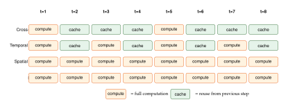
Distillation Pipeline
Consistency distillation (Definition 53) is one instance of a broader family of distillation approaches. The general idea is to train a “student” model that mimics the output of a “teacher” model (the full multi-step sampler) in fewer steps.
Definition 55 (Progressive Distillation for Video).
Progressive distillation [30] trains a sequence of student models, each reducing the step count by half:
Start with a teacher model that generates videos in steps.
Train a student model to match the teacher's output in steps, by learning to predict the result of two teacher steps in a single student step.
Use the student as the new teacher and repeat, halving the step count at each round.
After rounds, the final student generates in steps. The training objective at each round is (Progressive Distill) where denotes the stop-gradient operator and is the effective velocity obtained by running two teacher steps from .

Combining Acceleration Strategies
The three acceleration strategies described above are complementary and can be combined for multiplicative speedup:
Step reduction (consistency distillation or progressive distillation): reduce from 50 steps to 4 to 8 steps, yielding to speedup.
Feature caching (PAB + T-GATE): reduce the cost per step by to through selective reuse of attention outputs.
Higher-order solvers (DPM-Solver, Heun): achieve the same quality with to fewer steps than Euler.
Example 36 (Combined acceleration).
Consider a baseline video DiT that generates a 5-second, 720p video in 50 Euler steps, taking 200 seconds total (4 seconds per step). Applying the three strategies:
Consistency distillation to 8 steps: seconds.
PAB caching ( speedup per step): seconds.
These combined yield roughly speedup: from 200 seconds to 18 seconds.
This brings the generation time into a range that is practical for interactive applications, though still far from real-time.
Caution.
Each acceleration strategy introduces a quality-speed tradeoff. Consistency distillation can blur fine details. Feature caching can introduce temporal artifacts if the caching threshold is too large. Higher-order solvers can amplify numerical errors at very few steps. The optimal combination depends on the target application: a social media platform may tolerate some quality reduction for faster generation, while a film production pipeline demands the highest possible quality and can afford longer generation times.
Exercise 28 (Caching analysis).
A video DiT has transformer blocks. Each block has 4 sub-components: spatial self-attention (SA), temporal self-attention (TA), cross-attention (CA), and a feed-forward network (FFN). The compute cost of each sub-component is: SA = 40%, TA = 25%, CA = 15%, FFN = 20% of the total per-block cost.
If cross-attention is cached every 4 steps and temporal attention is cached every 2 steps (all other components computed every step), what is the average per-step compute saving?
If the total generation uses steps, what is the overall speedup compared to no caching?
What constraint does Proposition 31(ii) place on the caching threshold if the maximum acceptable per-step velocity error is and the tail Lipschitz constant is ? Why would it be a mistake to propagate this through (Caching Accum) to certify the error in the final sample?
Exercise 29 (Consistency model boundary condition).
The consistency model must satisfy (identity at the clean endpoint ; see Remark 49).
Why is this boundary condition necessary? Hint: is supposed to map any point of a trajectory to that trajectory's clean endpoint, and at the input is the clean endpoint.
A common implementation enforces this by parameterising , where and . Propose smooth functions and that satisfy these boundary conditions.
Show that your proposed parameterisation automatically satisfies the boundary condition regardless of the network output .
Training at Scale
Training a state-of-the-art video diffusion model is one of the most resource-intensive tasks in machine learning. The models contain billions of parameters, the training data consists of millions of video clips, and the training runs consume thousands of GPU-days. Naive approaches (randomly initialising a large model and training it end-to-end on full-resolution video) are both wasteful and unstable. Instead, every successful video generation system uses a carefully staged training procedure that progressively increases the resolution, duration, and complexity of the training data.
In this section, we formalise the multi-stage training paradigm, derive a transfer learning bound that explains why image pretraining helps, and describe the progressive resolution curriculum used by leading systems.
Multi-Stage Training
The multi-stage training paradigm decomposes the video generation training process into a sequence of stages, each building on the previous one.
Definition 56 (Multi-Stage Training Objective).
A multi-stage training procedure consists of stages , where is the training dataset at stage , specifies the resolution (frame count, height, width), and is the training objective. The model parameters at stage are initialised from the previous stage: (Multi Stage INIT) where are the optimised parameters from stage . The resolution increases across stages: (Resolution Progression)
The typical progression for a modern video generation system is:
Stage 1: Image pretraining. Train (or fine-tune) the model on a large dataset of images, treating each image as a single-frame “video.” This stage teaches the model spatial generation (objects, textures, composition) using the abundant supply of image data.
Stage 2: Low-resolution video. Extend the model to short video clips at low resolution (e.g., 16 frames at ). The temporal layers (temporal attention, temporal convolutions) are initialised randomly or from a motion module. This stage teaches basic motion and temporal coherence.
Stage 3: Medium-resolution video. Increase the resolution and duration (e.g., 33 frames at ). The model learns finer motion details and higher-quality spatial features.
Stage 4: High-resolution video. Train at the target resolution (e.g., 65 frames at or ) on a curated, high-quality dataset. This final stage refines the model's output quality.
Key Idea.
Image pretraining provides a massive head start. The spatial structure of video frames is essentially the same as the structure of natural images: objects, textures, lighting, and composition follow the same statistical regularities. By pretraining on images (of which billions are available), the model learns strong spatial priors before it ever sees a video. The subsequent video stages need only learn temporal dynamics (motion, temporal coherence, physics), which requires far less data and compute than learning spatial structure from scratch. This explains why even a model fine-tuned on “only” a few million videos can produce photorealistic output: it inherits spatial knowledge from image pretraining.
Transfer Learning Bound
Why does image pretraining help with video generation, and what exactly is left for the video stages to learn? The following theorem answers both questions by splitting the video score into a per-frame part - which an image model already supplies - and a temporal correction, and then computing the size of the correction in a tractable model.
Theorem 8 (Score Decomposition and the Size of the Temporal Correction).
Write a latent video as with , let be the law of the noisy video at time and the law of one noisy frame under the (common) single-frame marginal. Then the video score decomposes blockwise - not as a sum of -vectors - as (Score Decomp) where and is the dependence ratio. (Score Decomp) is an identity, not an approximation. Moreover, in the Gaussian model in which the centred frames have covariance with , , and the forward process is variance-preserving with :
Writing for the eigenvalues of , (Temporal Correction)
The correction vanishes identically if and only if , i.e. if and only if the frames are independent. Its relative size is bounded by (Temporal Correction Bound) with the temporal redundancy factor of (Temporal Redundancy) - the same quantity that sets the schedule shift in Theorem 6.
The relative size is increasing in : it vanishes as (high noise) and increases to as (clean data), which for and equals .
Proof.
The decomposition is the identity differentiated with respect to the block ; only the term of the sum survives, which is why the statement is blockwise and the right-hand side of (Score Decomp) lives in for each , the whole object living in .
For the Gaussian model, the noisy video has covariance , whose eigenvalues are , each of multiplicity ; the noisy per-frame marginal has covariance because and . Hence and the full score is , so and (TEMP CORR Trace) which is (Temporal Correction) after substituting ; and .
For (ii), every term of (Temporal Correction) vanishes iff for all , i.e. . For the bound, use (as ) to get , and note that by (Temporal Redundancy), while .
For (iii), each term is increasing in for , and is increasing in ; at the sum is . For the AR(1) correlation matrix, , giving the stated limit.
Remark 57.
Theorem 8 is worth reading carefully, because the intuitive story runs the other way round.
Coherent video needs more temporal correction, not less. The correction is exactly zero only for temporally independent frames, and it grows without bound as becomes singular: for the clean-data correction is already about times the squared norm of the image score, and at about times. Strong temporal coherence is a strong constraint, and a constraint is precisely what a product of per-frame marginals cannot express. What image pretraining transfers is the -dimensional per-frame part of (Score Decomp) - which is most of the parameters and most of the training compute - not the temporal coupling.
The correction is concentrated at low noise. By part (iii) it is negligible when and largest near the clean end. In the Gaussian model, the high-noise part of the trajectory is essentially inherited from the image model, and video-specific capacity is spent near the data end. This is a statement about second-order structure only: motion and occlusion are not Gaussian phenomena, and a model that is temporally correct to second order can still generate physically impossible motion.
The bound scales with and with . Longer and higher-resolution videos, and more coherent footage, need more video-specific training to learn the correction accurately.
Progressive Resolution Curriculum
The resolution progression from low to high is not merely a convenience; it provides a coarse-to-fine learning signal that stabilises training and improves final quality.
Example 37 (Progressive training curriculum (Open-Sora style)).
tab:vdiff:curriculum shows a typical progressive training curriculum inspired by Open-Sora [31] and CogVideoX [17].
tableProgressive training curriculum for video generation.
Each stage increases resolution and/or duration while decreasing
the batch size to fit within GPU memory.
Stage Data type Resolution Frames Batch Steps 1 Images 1 2048 200K 2 Images 1 1024 100K 3 Videos 16 256 150K 4 Videos 32 64 150K 5 Videos (HQ) 65 16 100K
Several design choices govern the curriculum:
Image stages precede video stages. Stages 1 and 2 train only on images, building spatial generation capability. The temporal layers are either absent or frozen during these stages.
Resolution increases gradually. Jumping directly from to often leads to training instability (loss spikes, mode collapse). Intermediate steps allow the model to adapt its spatial features progressively.
Frame count increases with resolution. At low resolution, training with many frames is computationally feasible and teaches long-range temporal coherence. At high resolution, memory constraints limit the frame count, but the temporal knowledge from earlier stages transfers.
Batch size decreases as resolution increases. GPU memory is the binding constraint, so the number of samples per step falls as each sample grows. It does not fall fast enough to hold the work per step fixed: for tab:vdiff:curriculum the total pixels processed per optimisation step are , , , and for stages 1 to 5 - a monotone sevenfold increase. Later stages are therefore more expensive per step as well as per sample, which is why they are also the shortest.
High-quality data in later stages. Early stages can use large, noisy datasets (web-scraped videos). Later stages use smaller, carefully curated datasets with high aesthetic quality, stable motion, and accurate captions.
Mixed Image-Video Training
A key practical technique is to mix image and video data within the same training batch, even during video-focused stages. This prevents catastrophic forgetting of spatial generation quality during video fine-tuning.
The mixed training objective is: (Mixed LOSS) where controls the mixing ratio and is the flow matching loss. Images are treated as single-frame videos () and processed by the same model architecture, with the temporal attention layers receiving a single token in the temporal dimension.
Remark 58.
The mixing ratio is typically set between 0.5 and 0.8, with the exact value depending on the relative sizes of the image and video datasets. CogVideoX uses in the video training stages, while Movie Gen [32] uses a curriculum where increases from 0.3 in early stages to 0.9 in late stages. The key insight is that some image data should always be present in the training mix, even in the final high-resolution video stage, to prevent spatial quality degradation.
Remark 59.
Modern video models must handle multiple aspect ratios (16:9, 9:16, 1:1, 4:3, etc.) to support different output formats. This is achieved by bucketing: the training data is grouped into aspect-ratio buckets, and each mini-batch draws from a single bucket so that all samples have the same spatial dimensions (enabling efficient batched computation). The model learns resolution and aspect-ratio awareness through positional encodings that encode the absolute coordinates within the video frame.
Data Curation
The quality of the training data is at least as important as the model architecture and training recipe. Video data from the web is noisy, poorly captioned, and highly variable in quality. Careful curation is essential.
Example 38 (Video data curation pipeline).
A typical data curation pipeline includes the following stages:
Collection. Crawl video data from the web or license proprietary datasets. Raw datasets may contain tens of millions of clips.
Safety filtering. Remove content that is unsafe, illegal, or violates content policies. This typically uses both automated classifiers and human review.
Technical filtering. Remove videos with: itemize
Very low resolution ().
Excessive compression artifacts.
Static content (e.g., slideshows, still images with music).
Excessive camera shake or motion blur.
Watermarks or overlaid text covering more than 10% of the frame. itemize
Aesthetic scoring. Assign an aesthetic quality score to each clip using a trained aesthetic predictor. Retain only clips above a threshold (e.g., top 30% to 50%).
Temporal quality scoring. Evaluate temporal coherence using metrics such as optical flow smoothness, scene-cut frequency, and inter-frame SSIM. Remove clips with excessive scene cuts or temporal artifacts.
Captioning. Generate detailed text descriptions for each clip using a vision-language model (e.g., a fine-tuned LLaVA or CogVLM). The captions should describe the visual content, actions, camera motion, and temporal progression.
Deduplication. Remove near-duplicate clips (which are common in web-scraped data) using perceptual hashing or learned embeddings.
After the full pipeline, the dataset typically shrinks to 10% to 30% of its original size, but the remaining clips are of substantially higher quality.
Remark 60.
The quality of text captions is critical for text-conditioned video generation. Poorly captioned data teaches the model to ignore the text conditioning (since the text provides no useful signal), leading to low text-video alignment at inference time. Several systems (Movie Gen, CogVideoX) invest heavily in caption quality, using multi-stage captioning pipelines that generate both short summaries and detailed frame-by-frame descriptions.
Scaling Laws and Compute Budgets
The relationship between model size, data size, and generation quality for video diffusion models is an active area of research. While precise scaling laws analogous to the Chinchilla scaling laws for language models have not yet been established, several empirical observations guide practice.
Example 39 (Compute budgets for recent systems).
tab:vdiff:compute-budgets provides estimated compute budgets for several prominent video generation systems.
tableEstimated model sizes and compute budgets for recent video
generation systems. GPU-hours are approximate and based on public
reports or estimates.
System Parameters GPU type Est. GPU-hours Open-Sora 1.2 1.1B H100 50K CogVideoX 5B A100 200K Stable Video Diffusion 1.5B A100 150K Movie Gen 30B H100 1M+ Sora (est.) 3B+ H100/A100 1M+
Remark 61.
Empirically, the following trends have been observed:
Model size improves quality sub-linearly. Doubling model parameters typically improves FVD by 10% to 20%, with diminishing returns beyond 5 to 10 billion parameters (for current architectures).
Data quality matters more than data quantity. Training on 2 million high-quality, well-captioned clips often produces better results than training on 20 million poorly-captioned, low-quality clips.
Longer training helps, up to a point. Most systems see continuous improvement up to 200K to 500K training steps per stage, with diminishing returns beyond.
Image pretraining provides the largest single improvement. Initialising from an image model (rather than random initialisation) typically improves final video quality by 30% to 50% (measured by FVD), while also reducing training time by 2 to 4.
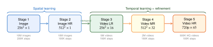
Practical Training Considerations
Beyond the high-level training pipeline, several practical considerations are critical for training video diffusion models at scale.
Learning rate scheduling. Each stage typically uses a warmup period (1K to 5K steps) followed by cosine decay. The peak learning rate often decreases across stages (e.g., for image pretraining, for low-resolution video, for high-resolution video) to prevent overwriting the knowledge from earlier stages.
Gradient accumulation. At high resolution, the batch size per GPU is severely limited (often 1 to 2 videos). Gradient accumulation across multiple micro-batches is used to achieve an effective batch size of 16 to 64, which is necessary for stable optimisation.
Model parallelism. For models exceeding 5B parameters, single-GPU training is impossible. Tensor parallelism (splitting layers across GPUs), sequence parallelism (splitting the token sequence), and pipeline parallelism are all used. The Open-Sora project [31] provides implementations of these parallelism strategies specifically optimised for video DiT models.
Noise schedule adaptation. The noise schedule (Noise Schedules for Video) must be adjusted at each stage to account for the changing resolution. As the resolution increases, the log-SNR shift from Proposition 28 increases in magnitude, requiring the schedule to be shifted toward higher noise levels.
EMA for sampling. An exponential moving average of the model weights is maintained throughout training and used for evaluation and sampling. The EMA decay rate is typically 0.9999 to 0.99999, with lower decay (faster averaging) in early stages and higher decay (slower averaging) in later stages where the model is closer to convergence.
Caution.
Training at scale is prone to instabilities. Common failure modes include:
Loss spikes during resolution transitions, caused by the sudden change in input statistics. Mitigation: use a warmup period at each new stage and gradually increase the learning rate.
Mode collapse in later stages, where the model produces only a narrow range of outputs. Mitigation: maintain sufficient data diversity and use a mixed image-video training objective.
Catastrophic forgetting of spatial quality during video fine-tuning. Mitigation: include image data in all training stages (Mixed Image-Video Training).
Numerical overflow in attention computations at high resolution, caused by large attention logits. Mitigation: use query-key normalisation () and mixed-precision training with careful loss scaling.
Exercise 30 (Multi-stage training analysis).
A video generation system uses the following 4-stage training curriculum on a cluster of 256 H100 GPUs:
Images at , batch size 2048, 200K steps.
Images at , batch size 1024, 100K steps.
Videos (), batch size 128, 150K steps.
Videos (), batch size 32, 100K steps.
Assume each forward-backward pass takes 0.5s per image at and scales quadratically with spatial resolution and linearly with frame count.
Compute the time per step at each stage (assuming perfect data parallelism across 256 GPUs).
Compute the total training time in GPU-hours for each stage.
What fraction of the total compute is spent on video training (stages 3 and 4)?
The stage-3 clips have latent frames with AR(1) temporal correlation , . Compute the temporal redundancy factor from (RF Exponential) with , then use (Temporal Correction Bound) to bound the relative magnitude of the temporal correction at and at . Which end of the trajectory does video-specific training have to work hardest at, and what does that imply for the timestep weighting of Remark 52? Answer for checking: ; the bounds are and respectively.
Exercise 31 (Data curation impact).
A team has collected 10 million web-scraped video clips, of which 30% are high-quality (sharp, well-lit, smooth motion, accurate captions) and 70% are low-quality (blurry, poorly captioned, with artifacts).
If the team trains on all 10M clips for 200K steps with batch size 64, how many epochs does training complete?
If instead they filter to only the 3M high-quality clips and train for the same number of steps, how many epochs does training complete?
Based on the empirical observation that “data quality matters more than data quantity,” which approach would you expect to produce better results? Justify your answer qualitatively.
Propose a curriculum that uses both subsets: the full 10M clips for early stages and the curated 3M clips for later stages. What advantages might this approach offer?
Summary and Looking Ahead
This section has covered the core training methodology for large-scale video diffusion models. The key insights are:
Noise schedules must adapt to the redundancy of video data (Noise Schedules for Video). The log-SNR curve is shifted downward; the dimension-counting rule is the perfectly-redundant limit and is a good approximation on the spatial axes, while on the temporal axis the factor should be replaced by the measured redundancy of Theorem 6.
Flow matching is the dominant training paradigm (Flow Matching for Video). The OT path provides straight trajectories that enable efficient sampling, and the v-prediction parameterisation is numerically stable across all timesteps.
Sampling acceleration is essential for practical deployment (Sampling Acceleration). Consistency distillation, temporal feature caching, and higher-order solvers combine to yield order-of-magnitude speedups.
Multi-stage training with image pretraining is the established recipe (Training at Scale). Progressive resolution curricula, mixed image-video training, and careful data curation are all critical for achieving state-of-the-art quality.
We turn next to the third pillar, control. The following sections develop classifier-free guidance in the multi-condition setting that video demands, image-to-video synthesis, camera control through Plücker ray conditioning, video ControlNets for structural conditioning, LLM-based prompt enhancement in the text-to-video pipeline, and parameter-efficient personalisation with LoRA, DreamBooth and their quantised variants. Evaluation - the Fréchet Video Distance, VBench and human protocols - is taken up later, once there is something to evaluate.
Classifier-Free Guidance for Video
Classifier-free guidance (CFG) has become the default mechanism for improving sample quality in diffusion models. In the image domain, the idea is straightforward: during training, randomly drop the conditioning signal and learn both a conditional and an unconditional denoiser; at inference, extrapolate away from the unconditional prediction toward the conditional one. For video, the situation is considerably richer because the conditioning signal is no longer a single text prompt. A video diffusion model may be conditioned on text descriptions, reference images, camera trajectories, motion maps, audio tracks, or any combination of these. Each conditioning modality carries different information and may warrant a different guidance strength.
In this section, we formalise multi-condition CFG for video, establish its Bayesian interpretation, describe the dropout schedules used during training, and illustrate the geometric intuition behind guided denoising.
Review: Single-Condition CFG
We begin with a brief review of the single-condition case, following [62]. Let denote a noise-prediction network conditioned on signal , and let denote the same network evaluated with the conditioning signal replaced by a null token . The guided noise prediction is (CFG Single) where is the guidance scale. When , we recover the standard conditional prediction. When , we amplify the “direction” from the unconditional prediction toward the conditional one, producing samples that are more strongly aligned with at the cost of reduced diversity.
Remark 62 (Score-function interpretation).
Recall that the noise prediction relates to the score function via . Substituting into (CFG Single), the guided score becomes (CFG Score) which is the score of the tempered distribution . For , this sharpens the conditional distribution; for , it broadens it toward the prior.
Multi-Condition CFG for Video
In video generation, the model typically receives multiple conditioning signals simultaneously. A text-to-video model conditioned on text and a reference image must balance fidelity to the textual description against visual consistency with the reference frame. Adding camera parameters or motion trajectories introduces further dimensions of control.
Definition 57 (Multi-Condition CFG).
Let be a set of conditioning signals, each with its own guidance weight . The multi-condition classifier-free guidance prediction is (Multi CFG) where denotes the prediction with only condition active (all other conditions replaced by ), and is the fully unconditional prediction.
For the common case of text and image conditioning, this becomes (CFG TEXT IMG) where we suppress the time argument for brevity. This formulation allows independent control over how strongly the generated video aligns with the text description versus the reference image. Systems that accept both a prompt and a reference frame - image-animation and video-continuation models - expose exactly this pair of dials, and the two weights are almost never equal: the reference frame pins down appearance, layout and lighting exactly, whereas the prompt constrains only what is described in words. A weaker weight on the more informative condition is therefore the usual setting; Example 41 collects the ranges that are typical in practice.
Remark 63 (Two conventions for the guidance scale).
(CFG Single) is written so that reproduces the plain conditional prediction and the unconditional one. Part of the literature instead writes , in which is the conditional prediction. The two scales differ by one, , so a quoted numerical range is meaningless without knowing which convention it uses. Every number in this chapter follows (CFG Single).
Guidance need not be a single scalar shared by the whole clip. The noise tensor has a frame axis, and nothing forces the guidance weight to be constant along it.
Example 40 (Frame-axis guidance in Stable Video Diffusion).
Stable Video Diffusion [8] is a useful corrective to the two-weight picture above, because its released image-to-video models have no text pathway at all: the CLIP text embedding of the underlying image model is replaced wholesale by the CLIP image embedding of the conditioning frame, and the conditioning frame is additionally concatenated channel-wise to the denoiser input. There is therefore a single condition and a single guidance weight - no exists to be traded against a .
What SVD varies instead is the guidance weight along the frame axis. A constant scale is unsatisfactory in both directions: too little guidance and the later frames drift away from the conditioning image, too much and the early frames - which are nearly copies of a frame the model already has - oversaturate. SVD therefore increases the scale linearly across the frame axis, from roughly at the first generated frame to roughly at the last. In the notation of Definition 60 this is a weight indexed by frame rather than by diffusion time: (SVD Frame Guidance) The pattern is worth naming because it generalises: the guidance weight is a function on the whole grid, and video models exploit all three axes.
Caution.
Over-guidance degrades temporal coherence. In image diffusion, high guidance scales produce saturated, “HDR-like” artefacts. In video, the failure mode is more severe: over-guidance introduces temporal flickering, where each frame is individually sharp but adjacent frames are inconsistent. This occurs because the guidance amplifies per-frame conditional alignment at the expense of the inter-frame correlations captured by the unconditional model. Video systems consequently run at somewhat lower guidance scales than image systems, and lower still on conditions that are already highly informative; see Example 41 for typical ranges.
Compositional Guidance
The multi-condition formulation in Definition 57 treats each conditioning signal independently: the guidance directions are summed without accounting for potential interactions. A more nuanced approach considers joint conditioning, where some combinations of conditions are dropped together.
Definition 58 (Compositional Guidance Schedule).
Let be a collection of subsets of conditions. For each subset , let denote the prediction with conditions active and all others set to . The compositional guidance prediction is (Compositional CFG) where is the guidance weight for subset .
For two conditions (text and image), the compositional formulation includes three guidance terms: text only, image only, and joint text-plus-image. With appropriate weights, this captures synergistic effects that the additive formulation in (Multi CFG) misses.
Remark 64 (Computational cost of compositional guidance).
Each term in (Compositional CFG) requires a separate forward pass through the denoiser network. With subsets (including the unconditional pass), the cost per denoising step is multiplied by . For two conditions, the full compositional expansion requires forward passes (the unconditional pass, text-only, image-only, and joint), compared to passes for the additive scheme. This cost grows exponentially with , making full compositional guidance impractical for more than two or three conditions. In practice, most systems use the additive formulation with carefully tuned per-condition weights.
CFG as Approximate Bayesian Inference
The score-function viewpoint in Remark 62 hints at a deeper probabilistic interpretation. We now formalise this.
Theorem 9 (CFG as Tempered Posterior Sampling).
Let be the unconditional data distribution and the conditional distribution. Define the tempered posterior (Tempered Posterior) Then at the guided score is exactly the score of the tempered posterior, and at the identity is taken as the definition of the guided score at that noise level: (Tempered Score) In particular, the CFG sampling process with guidance weight targets rather than the true conditional .
Proof.
By Bayes' rule, . Substituting into (Tempered Posterior), Taking the log and differentiating with respect to : The conditional score decomposes as , so . Substituting: This establishes (Tempered Score) at .
Caution.
The tempered posterior does not survive noising. It is tempting to conclude that the same decomposition holds at every noise level, on the grounds that the forward process is applied independently of . It does not. Adding noise is a convolution and geometric tempering is a pointwise power, and the two operations do not commute: (Tempering Noncommute) in general. What CFG actually does at is take (Tempered Score) as a definition of the guided vector field and integrate it; the marginal that this sampler produces at agrees with only approximately. The tempered posterior is therefore the right intuition for what guidance does, not an exact characterisation of what it samples. This is worth stating plainly because the mismatch is one of the reasons large guidance weights degrade sample statistics in ways the tempering picture does not predict.
Insight.
Guidance as temperature control. The tempered posterior raises the likelihood to the power . For , modes of the likelihood are amplified, concentrating the distribution around samples that most strongly match the condition . This is analogous to reducing the temperature in a Boltzmann distribution, trading diversity for quality. For video, this trade-off is particularly consequential: high guidance sharpens per-frame fidelity but can destroy the smooth temporal transitions that characterise natural video.
Multi-Condition Extension
For multiple conditions, the Bayesian interpretation extends naturally under a conditional independence assumption.
Proposition 32 (Multi-Condition Tempered Posterior).
Assume the conditions are conditionally independent given , i.e., . Then the multi-condition CFG prediction in (Multi CFG) corresponds to sampling from the tempered posterior (Multi Tempered)
Proof.
Under conditional independence, the joint conditional score decomposes as Replacing each conditional score difference with its weighted version and collecting terms yields the score of .
This result provides principled guidance for choosing the weights : each weight controls the “temperature” of the corresponding likelihood term. Setting recovers the standard posterior contribution from condition ; amplifies it; ignores it entirely.
Example 41 (Weight selection heuristics).
The following ranges are typical defaults in released video systems, all quoted in the convention of (CFG Single) (see Remark 63):
Text-to-video: , somewhat lower than the scales used for text-to-image, to preserve temporal coherence.
Image-to-video: , lower than text guidance because the image already provides strong structural constraints.
Camera-conditioned: , camera conditions are geometric and tolerate less amplification before introducing perspective distortions.
Motion trajectories: , higher values enforce stricter adherence to the specified motion paths.
These ranges are rules of thumb rather than measured optima: they are defaults that ship with public implementations, and they vary with the architecture, the noise schedule and the guidance convention. Treat them as starting points to be tuned, not as constants. The transferable principle is that stronger conditioning signals - those that more precisely constrain the output - require lower guidance weights, while weaker signals benefit from amplification.
Training with Conditional Dropout
For CFG to work, the model must be trained to handle missing conditions. This is achieved by randomly dropping conditions during training with specified probabilities.
Definition 59 (Multi-Condition Dropout Schedule).
Let be per-condition dropout probabilities and the probability of dropping all conditions simultaneously. During training, at each step, the conditioning configuration is sampled as follows:
With probability , set all conditions to (fully unconditional training).
Otherwise, for each condition independently, replace with with probability .
This produces a mixture of training examples with various subsets of active conditions.
Example 42 (Dropout rates in practice).
Typical dropout rates for video diffusion models:
| Condition | Notes | |
| Text caption | 0.10–0.15 | Standard for text-conditional models |
| Reference image | 0.05–0.10 | Lower because image is critical |
| Camera pose | 0.10–0.20 | Can be higher; camera is auxiliary |
| Motion map | 0.10–0.20 | Similar to camera |
| All conditions | 0.05 | Small but essential for unconditional baseline |
Remark 65 (Joint versus independent dropout).
The training dropout schedule should be designed so that the model encounters all the conditioning configurations that will be needed at inference time. For the additive multi-condition CFG in (Multi CFG), the model needs to evaluate for each individually, as well as . This means the model must see training examples with exactly one condition active. Independent dropout naturally produces such examples, but with probability , which may be small for large . Some training schedules explicitly sample single-condition configurations to ensure adequate coverage.
Dynamic Guidance Schedules
A constant guidance scale throughout the denoising process is suboptimal. Early denoising steps (high noise) determine large-scale structure; late steps (low noise) refine fine details. Applying the same guidance weight at both stages can lead to over-saturation in the details or under-specification of the structure.
Definition 60 (Time-Dependent Guidance Schedule).
A time-dependent guidance schedule replaces the constant weight with a function . The guided prediction at time is (Dynamic CFG) Sampling runs from (pure noise) down to (clean data), so a schedule is characterised by which end of that range carries the larger weight. Writing for the fraction of the trajectory already completed, the common families are:
Linear ramp: , which is weakest at high noise and strongest as the sample resolves. Reversing the sign of the slope gives the front-loaded variant, strongest at high noise.
Cosine schedule: , the same monotone progression with a smooth start and end (again reversible).
Step schedule: for and for , with a hard transition at threshold .
Both directions are in use, and which one is right is a property of the modality rather than a universal truth. Image samplers often front-load guidance, on the reasoning that the high-noise steps choose the semantic content and therefore need the strongest push towards the prompt. For video the argument frequently runs the other way: temporal coherence is settled during the early, high-noise steps, when the model commits to an overall motion trajectory and scene layout, and strong guidance at that point distorts the motion field by over-weighting per-frame conditional alignment at the expense of the inter-frame correlations that only the unconditional branch carries. On that reasoning the guidance is kept modest while the motion is being decided and raised once the layout is fixed and only per-frame detail remains.
Key Idea.
Decide motion under weak guidance, sharpen detail under strong guidance. The failure mode that dynamic schedules exist to avoid is guidance-induced flicker, and flicker is created early, when the motion field is set. A schedule that is weak at high noise and strong at low noise therefore lets the model establish a coherent trajectory first and match the conditioning signal second. The converse profile buys sharper prompt adherence at the cost of temporal stability. Which trade you want is a product decision, not a mathematical one; what matters is that a constant weight makes the trade without being asked.
Geometric Illustration of CFG
The following diagram illustrates the geometry of multi-condition CFG. The unconditional denoising direction, the text-conditional direction, and the image-conditional direction are vectors in the latent space. CFG forms a weighted combination of the differences between the conditional and unconditional directions.
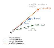
Negative Prompts and Guidance Rejection
An extension of CFG replaces the unconditional prediction with a negative prompt prediction. Instead of extrapolating away from , we extrapolate away from , where is a text description of undesired attributes (e.g., “blurry, low quality, jittery motion, deformed hands”).
(Negative Prompt)
For video, negative prompts are especially useful for suppressing common artefacts such as temporal flickering, morphing faces, and physically implausible motion. The negative prompt effectively steers the denoising trajectory away from the manifold of low-quality videos, complementing the positive guidance that steers toward the desired content.
Exercise 32 (Negative prompt as modified prior).
Show that using a negative prompt in place of the null token in CFG corresponds to sampling from a modified distribution . Discuss the conditions under which this produces better samples than standard CFG.
Image-to-Video Synthesis
One of the most practically useful modes of video generation is image-to-video (I2V) synthesis: given a single still image, generate a plausible video that “brings the image to life.” The input image provides a strong visual prior (appearance, layout, lighting, identity of objects), and the model must hallucinate coherent motion, camera dynamics, and temporal evolution consistent with both the image and an optional text description.
Image-to-video synthesis is central to creative workflows (animating photographs, concept art, and product images), visual effects (creating establishing shots from matte paintings), and scientific visualisation (simulating dynamics from initial conditions). It is also a stepping stone toward longer video generation, where autoregressive approaches generate each clip conditioned on the last frame of the previous clip.
In this section, we formalise the I2V problem, describe the conditioning mechanisms used by state-of-the-art systems, and analyse how information from the first frame propagates through the network.
Problem Formulation
Definition 61 (Image-to-Video Conditioning).
Let be the latent encoding of the first frame (the conditioning image), and let denote the latent codes of the remaining frames. The image-to-video generation task is to sample from the conditional distribution (I2V Distribution) where is an optional text prompt describing the desired motion and scene dynamics. The first frame is fixed (given), and frames through are generated.
The quality of an I2V model is measured along three axes: (i) visual fidelity of each generated frame, (ii) temporal coherence of the motion across frames, and (iii) identity preservation of objects, textures, and lighting established by the conditioning image. The third axis distinguishes I2V from text-to-video: the generated video must look like a natural continuation of the specific input image, not merely a plausible video matching the text description.
Conditioning Mechanisms
There are three principal mechanisms for injecting the first-frame information into the diffusion model: concatenation conditioning, cross-attention conditioning, and hybrid approaches that combine both.
Concatenation conditioning
The most direct approach concatenates the clean first-frame latent with the noised latents of the remaining frames along the channel dimension.
Definition 62 (Concatenation I2V Conditioning).
Let be the noised latent stack over all temporal positions, and let denote the clean first-frame latent broadcast along the temporal axis. At each denoising step, construct the augmented input tensor (I2V Concat) where the concatenation is along the channel axis. The denoiser operates on this augmented tensor, , and its prediction at temporal position is discarded: that frame is given, not generated, so it contributes neither to the sample nor to the training loss (Exercise 33).
Broadcasting is not the only option. A variant places the clean latent only at the first temporal position and a zero placeholder elsewhere, (I2V Concat SLOT) which is cheaper to describe but forces every later frame to reach the anchor through temporal mixing rather than reading it directly.
Either way, the extra channels widen the first convolutional layer of the denoiser, whose additional input weights are initialised to zero so that the pre-trained model is exactly recovered at the start of fine-tuning.
Stable Video Diffusion [8] uses the broadcast form of (I2V Concat), with one refinement: the conditioning latent is noise-augmented before concatenation, that is, a small amount of noise is added to and the corresponding noise level is supplied to the network. The purpose is to close the train/test gap - at inference the conditioning frame is a real photograph rather than a frame drawn from the training distribution - and to give the user a dial that trades fidelity to the input image against the amount of motion the model is willing to invent. (SVD Concat)
Remark 66 (Why the first frame is noise-free).
The crucial detail in I2V conditioning is that the conditioning latent enters the network at a noise level that does not follow : it stays clean, or nearly clean, while the frames being generated are noised at level . The asymmetry is intentional. The first frame is observed data, not a variable to be denoised, so holding it fixed gives the denoiser a stable reference signal at every step of the reverse process rather than one that degrades as grows.
“Nearly clean” rather than “clean” because a small fixed noise augmentation, as in (SVD Concat), is usually preferable to none: the encoder sees latents of user-supplied images that are not distributed like its training data, and a little noise both blurs that mismatch and, by weakening the anchor, lets the model produce more motion. The augmentation level is therefore exposed to users as a motion-strength control.
Cross-attention conditioning
An alternative to concatenation injects the first-frame information through cross-attention layers, analogous to how text embeddings are injected in text-to-image models. The first frame is encoded by a frozen image encoder (e.g., CLIP or DINOv2) to produce a sequence of image tokens , where is the number of spatial tokens. Each attention layer in the denoiser computes (I2V Crossattn) where are queries derived from the noised video latents.
Cross-attention conditioning is more parameter-efficient than concatenation (no additional input channels needed) and allows the model to selectively attend to different parts of the reference image at different frames and layers. However, it provides a more “semantic” representation of the first frame, which may lose fine-grained pixel-level details that concatenation preserves.
Hybrid conditioning
State-of-the-art I2V systems typically combine both mechanisms: concatenation for pixel-level detail and cross-attention for semantic guidance. This hybrid approach, used in systems such as Stable Video Diffusion [8] and DynamiCrafter [67], provides the denoiser with both low-level (exact pixel values of the reference frame) and high-level (semantic features extracted by a vision encoder) information about the conditioning image.
Key Idea.
Dual pathways for image conditioning. The most effective I2V architectures provide two pathways for first-frame information: (1) concatenation of the raw latent codes, which preserves exact pixel-level detail, and (2) cross-attention to image encoder features, which provides semantic and structural context. The concatenation pathway dominates at low noise levels (where fine details matter), while the cross-attention pathway dominates at high noise levels (where global structure is being determined).
Information Propagation from the First Frame
A fundamental question in I2V synthesis is: how does information from the first frame reach distant frames? If the model processes only local temporal neighbourhoods, frame may receive little influence from frame . The answer depends on the architectural choices of the denoiser.
Proposition 33 (First-Frame Information Flow).
Consider a video diffusion transformer with layers, each containing temporal self-attention with receptive field spanning all frames. Let denote the attention weight that frame assigns to frame at layer . Under the assumption that attention weights are approximately uniform at initialisation, the cumulative information from frame reaching frame after layers satisfies (INFO FLOW Bound) where is the fraction of frame 's representation that is influenced by frame . In particular, for , the information flow exceeds for all frames.
Proof.
At each layer, frame receives at least a fraction of information from frame through the uniform attention distribution. The fraction of information that has not been influenced by frame after layers is at most . Therefore, . For , we have , giving .
Remark 67 (How pessimistic the uniform-attention bound is).
Read literally, Proposition 33 is a discouraging result: driving the residual below takes layers, which for is about layers and for about - far deeper than any deployed video DiT. Real models are nowhere near that deep and first-frame conditioning works anyway, so the bound is loose, and it is worth being explicit about where the looseness comes from.
The premise is uniform attention, which is the worst case for this particular question: it is the initialisation, not the trained model. A trained I2V denoiser concentrates a large share of its temporal attention mass on the anchor frame, and once is a constant rather than the same argument gives - a genuinely logarithmic depth. The proposition is therefore best read as an argument for why trained attention must be non-uniform, rather than as a depth requirement.
For models with factored temporal attention (where each temporal attention layer has a limited window of frames), the information takes layers to propagate, which may require deeper networks. This trade-off between attention window size and network depth is a key architectural consideration in I2V models.
The non-uniformity has a characteristic shape: frames closer to the conditioning image attend to it more strongly, and the attention mass falls away with temporal distance. A convenient toy model is , under which frame attends about more strongly to the anchor than frame does. We use this profile below purely as an illustrative functional form - it is not a measurement of any particular released model, and the decay exponent varies with architecture, clip length and training data. The qualitative point it captures is the one that matters practically: the anchor's influence is strongest at the start of the clip and weakest at the end, which is exactly where identity drift is observed.
State-of-the-Art I2V Systems
We briefly survey three influential I2V systems that illustrate different design choices.
Stable Video Diffusion (SVD).
Blattmann et al. [8] extend the Stable Diffusion image model to video by inserting temporal attention layers between the existing spatial attention layers. The model is trained in three stages: (1) image pre-training, (2) video pre-training on a large but noisy dataset, and (3) video fine-tuning on a smaller, high-quality dataset - a curation argument as much as an architectural one, and the paper's main empirical claim is that the third stage is what separates a usable model from an unusable one. SVD generates 14–25 frames at resolution and serves as the backbone for many downstream I2V applications.
Its conditioning design is worth stating precisely, because it is often misdescribed. The released image-to-video models are purely image-conditioned. There are two pathways and neither of them carries text: the conditioning frame is concatenated channel-wise after noise augmentation ((SVD Concat)), and the CLIP text embedding that the underlying image model consumed through cross-attention is replaced by the CLIP image embedding of that same frame. A prompt has nowhere to enter, so SVD offers a single guidance weight rather than the text/image pair of (CFG TEXT IMG) - which is why the frame-axis ramp of Example 40 is where its guidance sophistication lives.
I2VGen-XL.
Zhang et al. [68] propose a cascaded I2V pipeline with two stages: a base model that generates low-resolution video from the input image, and a refinement model that upsamples to high resolution. The key insight is that the base model focuses on motion generation (getting the dynamics right), while the refinement model focuses on visual quality (sharpening textures and preserving identity). This decomposition allows each stage to be optimised independently.
DynamiCrafter.
Xing et al. [67] take a hybrid conditioning approach, combining concatenation with dual cross-attention to both CLIP image features and text features. A distinguishing feature is the use of a “visual context” module that extracts multi-scale features from the conditioning image and injects them at multiple layers of the denoiser. This provides richer structural information than single-scale cross-attention and helps preserve fine details across long temporal horizons.
I2V Pipeline Diagram
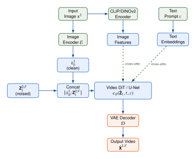
Exercise 33 (I2V training objective).
Write the explicit training loss for an I2V model that uses concatenation conditioning. Starting from the standard video diffusion loss , show how the first-frame conditioning modifies the input to the denoiser. Should the loss include the first frame? Argue that excluding the first frame from the loss computation (since it is given, not generated) is important for training stability.
Exercise 34 (Autoregressive video extension).
Explain how an I2V model can be used autoregressively to generate arbitrarily long videos. Given a video of frames generated from a conditioning image, describe how to use the last frame (or last few frames) as the conditioning image for the next clip. Discuss the challenges of drift (gradual degradation of quality and divergence from the original content) and propose at least two strategies to mitigate it.
Motion and Camera Control
Text prompts and reference images specify what should appear in a video, but they provide limited control over how the scene moves. A filmmaker does not merely describe “a dog running in a park”; they specify the camera angle, the tracking shot direction, the speed of the zoom, and the trajectory of the subject. This level of control requires conditioning signals that go beyond language and into the domain of geometry and physics.
In this section, we introduce two families of spatial control for video diffusion: camera control, which specifies the viewpoint trajectory, and motion control, which specifies the movement of objects within the scene. We formalise the mathematical representations used for each (Plücker coordinates for cameras, dense flow fields and sparse trajectories for motion) and describe the architectural mechanisms that inject these signals into the diffusion model.
Camera Representations
A camera in 3D space is characterised by its pose: a rotation matrix and a translation vector . Together, these define the rigid transformation from world coordinates to camera coordinates, (World TO CAM) For video, we have a sequence of camera poses , one per frame, defining the camera trajectory.
Caution.
is not the camera position. Under (World TO CAM) the camera centre is the world point that maps to the camera-frame origin, i.e. the solution of : (Camera Centre) Only when does , and never . Confusing with is the single most common error in ray-based camera conditioning, and it is a silent one: the resulting ray map is still smooth, still has the right shape, and still trains - it simply encodes the wrong camera trajectory. Some codebases store the camera-to-world transform instead, in which the translation column is the camera centre; the two conventions differ by exactly the inversion in (Camera Centre). Check which one a dataset uses before building a ray map from it.
The intrinsic parameters are captured by the camera matrix : (Intrinsic Matrix) where are the focal lengths in pixel units and is the principal point. For a pixel at coordinates in frame , the corresponding 3D ray direction in world coordinates is (RAY Direction)
While rotations and translations are sufficient to describe camera pose, they are not ideal as conditioning signals for neural networks. Rotations live on the non-Euclidean manifold , and naively encoding them as matrices introduces redundant parameters and discontinuities. Plücker coordinates provide a more natural parameterisation for camera rays.
Definition 63 (Plücker Coordinates for Camera Rays).
A 3D line through the camera centre with direction can be represented by its Plücker coordinates , where (Plucker D) where is the ray direction in world coordinates and is the moment of the ray about the world origin. The six-dimensional vector determines the line, is defined up to a common non-zero scale, and satisfies the constraint .
Remark 68 (Why Plücker coordinates?).
Plücker coordinates offer several advantages over raw camera parameters for neural network conditioning:
Per-pixel representation. Each pixel in the video maps to a unique 6D Plücker vector, creating a dense conditioning signal of shape that aligns naturally with the video tensor.
Continuity. Unlike rotation matrices (which have discontinuities under any 3D parameterisation due to the topology of ), Plücker coordinates vary smoothly as the camera moves along a smooth trajectory.
Encoding absolute geometry, not just orientation. The direction alone says where the ray points but not where it is; a pure rotation encoding cannot distinguish a camera that has translated sideways from one that has not moved. The moment supplies exactly the missing information: is the perpendicular distance from the world origin to the ray, and 's direction fixes the plane the ray lies in. The network therefore receives the ray's absolute placement in the scene, which is what parallax depends on.
Caution.
The moment does not recover the camera centre. It is tempting to read as “the moment encodes the camera position”, but it does not: sliding the origin of the ray along its own direction leaves the moment unchanged, since . Plücker coordinates describe a line, not a point on it, and the camera centre is recoverable only by intersecting the lines of two or more pixels of the same frame. This is a feature, not a defect - the conditioning signal is invariant to exactly the quantity that carries no geometric content - but it does mean that statements of the form “ encodes the camera position” are false as written.
The Plücker ray map for an entire video is a tensor , where the entry at contains the 6D Plücker coordinates of the ray from the -th camera through pixel . This tensor can be precomputed from the camera trajectory and intrinsics before generation begins.
Camera-Conditioned Diffusion
Definition 64 (Camera-Conditioned Diffusion).
A camera-conditioned video diffusion model takes as input the noised video latent , the diffusion timestep , and the camera trajectory , and predicts the noise: (CAM COND) The camera trajectory is injected into the model via one of the following mechanisms:
Plücker ray concatenation: Compute the Plücker ray map and concatenate it with the noised latent along the channel dimension: .
Camera embedding addition: Encode each frame's pose into a -dimensional vector via an MLP: , and add it to the timestep embedding or to the input of each temporal attention layer.
Camera ControlNet: Process the Plücker ray map through a parallel encoder network and inject the features into the main denoiser via zero-convolution (see Video ControlNet).
Example 43 (CameraCtrl).
CameraCtrl [33] adopts the Plücker ray concatenation approach. For each frame , the Plücker ray map is downsampled to match the spatial resolution of the latent space () and concatenated with the latent along the channel dimension. The first convolutional layer is expanded from input channels to channels, with the additional weights initialised to zero so that the pre-trained model is preserved at the start of fine-tuning.
The method is evaluated by running structure-from-motion on the generated clip, recovering the camera trajectory that the video actually depicts, and comparing it against the requested one; the reported errors are a rotation error and a translation error computed this way, both normalised so that trajectories of different scales are comparable. We do not quote figures here, because such numbers are only meaningful relative to a specific base model, trajectory set and pose estimator, and they are not comparable across papers. The qualitative finding is the transferable one: a six-channel geometric conditioning signal added to a frozen backbone buys usable trajectory control without measurably degrading visual quality.
Camera Ray Diagram
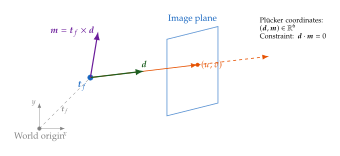
Motion Control via Trajectories and Flow
Camera control specifies how the viewpoint moves; motion control specifies how objects within the scene move. There are two principal representations for motion conditioning: sparse trajectories (a small number of control points with specified 2D paths) and dense optical flow (a per-pixel displacement field).
Sparse trajectory conditioning
A sparse trajectory specifies the motion of control points across frames: (Sparse TRAJ) where is the 2D position of control point in frame . The user specifies these trajectories (e.g., by drawing arrows on the first frame), and the model generates video where the corresponding image regions follow the specified paths.
DragNUWA [35] encodes sparse trajectories as a sequence of Gaussian heatmaps centred at each control point, producing a conditioning tensor of shape . Each channel corresponds to one control point, with the heatmap peak indicating the desired position at each frame.
Dense flow conditioning
Dense flow conditioning provides a per-pixel motion specification. The conditioning signal is an optical flow field for each consecutive pair of frames, specifying the 2D displacement of each pixel from frame to frame . This is the richest possible motion specification but requires the user (or an upstream motion planning module) to provide detailed per-pixel flow, which is rarely available in practice.
Remark 69 (Motion from language).
A middle ground between sparse user-specified trajectories and dense optical flow is to infer motion from the text prompt. Systems such as MotionCtrl [34] use a motion planner module (often an LLM or a specialised motion prediction network) to convert textual motion descriptions (“the ball rolls from left to right”) into trajectory or flow representations that condition the diffusion model. This bridges the gap between the ease of text input and the precision of geometric control.
Video ControlNet
ControlNet [69] is the dominant architecture for injecting structured spatial control into diffusion models. Originally designed for images (conditioning on edges, depth maps, pose skeletons), it extends naturally to video by processing spatiotemporal control signals.
Definition 65 (Video ControlNet).
Let be a pre-trained video diffusion model (the base model) with encoder blocks producing intermediate features . A Video ControlNet consists of a parallel encoder (a trainable copy of the base encoder) that processes the control signal and produces features . The features are combined via zero-convolution layers: (Controlnet) where is a convolution (or, for video, a convolution) initialised with all weights and biases set to zero: (ZERO INIT)
The zero initialisation is the key design principle of ControlNet. At the start of training, the zero-convolution layers output exactly , so the combined features and the model behaves identically to the pre-trained base model. As training progresses, the zero-convolution weights grow from zero, gradually introducing the control signal without disrupting the learned representations.
Insight.
Zero-convolution as controlled initialisation. The zero-convolution trick solves the “cold start” problem in fine-tuning: how to add new conditioning pathways to a pre-trained model without destroying its existing capabilities. By starting the control pathway at zero, training begins from the exact output distribution of the pre-trained model, and the control signal is introduced as a gentle perturbation that grows as the model learns to use it. This is far more stable than random initialisation of the control pathway, which would produce large, unstructured perturbations to the base model's features.
Proposition 34 (Training Stability of Zero-Convolution).
Let be the training loss of the base model (without control input) and let be the loss with ControlNet parameters and zero-convolution parameters . At initialisation (, ), (ZERO CONV INIT LOSS) and the gradient with respect to the zero-convolution parameters is the outer product (ZERO CONV GRAD) a matrix of the same shape as , whose Frobenius norm is exactly (ZERO CONV GRAD NORM) The initial gradient signal is thus the product of the base model's sensitivity and the control encoder's output magnitude, providing a natural scaling that prevents large initial perturbations.
Proof.
At and , the zero-convolution outputs , so and . For the linear map we have , so the chain rule gives , which is (ZERO CONV GRAD). For any outer product , , giving (ZERO CONV GRAD NORM) with equality rather than the inequality that submultiplicativity would supply.
Remark 70 (Zero weights do not mean zero gradients).
A reasonable worry about (ZERO INIT) is that a layer initialised to zero should be stuck there, as it would be if the zero-initialised parameter appeared on both sides of a product. (ZERO CONV GRAD) shows why it is not: the gradient depends on , which is produced by the separately initialised control encoder and is generically non-zero. The zero-convolution contributes nothing to the forward pass and a full gradient to the backward pass. This is the same mechanism that makes adaLN-Zero and LoRA's zero-initialised factor work (Remark 74), and it is the reason all three can be described as “starting as a no-op” without also being frozen.
ControlNet Architecture Diagram
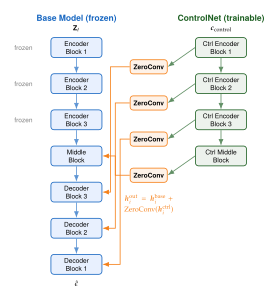
Types of Motion and Camera Control
We summarise the principal forms of spatial control for video diffusion and the systems that implement them.
| Control Type | Representation | Injection | System |
| Camera trajectory | Plücker rays | Concatenation / ControlNet | CameraCtrl [33] |
| Camera + object motion | Pose + flow | Dual ControlNet | MotionCtrl [34] |
| Drag-based motion | Sparse trajectories | Heatmap encoding | DragNUWA [35] |
| Character animation | Pose skeleton | Reference attention | AnimateAnyone [36] |
| Motion patterns | Learned motion LoRA | Adapter injection | AnimateDiff [37] |
MotionCtrl.
Wang et al. [34] propose a unified controller that handles both camera motion and object motion. Camera motion is encoded as per-frame pose embeddings added to the temporal attention layers. Object motion is encoded as sparse trajectory maps processed by a lightweight convolutional encoder. The two motion types are disentangled during training by alternating between camera-motion and object-motion supervision, allowing independent control at inference time.
AnimateAnyone.
Hu et al. [36] address the specific problem of character animation: given a single image of a person and a sequence of target body poses (represented as OpenPose skeletons), generate a video of that person performing the corresponding motion. The architecture uses a reference attention mechanism, where features from the reference image are injected into the temporal attention layers of the denoiser to preserve the identity and appearance of the subject.
Caution.
Motion control can conflict with text guidance. When both text prompts and explicit motion specifications (camera trajectories, sparse drags) are provided, they may specify conflicting dynamics. For example, the text “the camera pans slowly to the left” conflicts with a camera trajectory that moves right. In such cases, the model must resolve the conflict, and the result depends on the relative guidance weights. Practical systems typically give priority to explicit geometric control over textual descriptions, since geometric specifications are more precise and less ambiguous. Users should be warned to ensure consistency between text and motion inputs.
Mathematical Properties of Plücker Conditioning
We conclude the discussion of camera control with a proposition relating Plücker conditioning to the underlying 3D geometry.
Proposition 35 (Epipolar Constraint from Plücker Coordinates).
Let and be the Plücker coordinates of two rays emanating from camera centres and respectively, and assume the rays are not parallel (). The rays meet in a common 3D point if and only if the reciprocal product vanishes: (Reciprocal Product) This condition is equivalent to the classical epipolar constraint , where is the fundamental matrix and are the corresponding pixel coordinates.
Proof.
Let parameterise the first line and the second. They meet when for some , i.e. when lies in . Since that span is a plane with normal , so the condition is exactly (Coplanarity) Now expand the moments. Using the scalar triple product and its antisymmetry under swapping two arguments, so that (Reciprocal Identity) which vanishes precisely when (Coplanarity) holds. The equivalence to the fundamental-matrix constraint is a standard result in multi-view geometry.
Remark 71 (Why the non-parallel hypothesis is needed).
Drop the assumption and the “only if” direction fails. Two parallel but distinct rays - the same pixel of a camera undergoing pure sideways translation, for instance - have , so (Reciprocal Identity) makes the reciprocal product vanish identically, yet the rays never meet. What the vanishing reciprocal product characterises in full generality is coplanarity: the two lines are coplanar, hence either intersecting or parallel. For camera conditioning the distinction is mostly benign, since parallel correspondences are the degenerate case that also breaks triangulation, but the statement is worth getting right.
This proposition explains why Plücker coordinates are effective for camera conditioning: the network can learn to enforce multi-view consistency by learning functions of the reciprocal product, which directly encodes the geometric relationship between rays across frames.
Exercise 35 (Plücker coordinates for zoom).
Consider a camera that zooms in by changing its focal length from to while keeping the camera position and orientation fixed (, , hence camera centre for all ). Derive the Plücker coordinates for a pixel as a function of the focal length. Show that the moment vector for all rays (since the camera sits at the world origin, every ray passes through it), and the direction vectors change as . Explain how this representation allows the diffusion model to distinguish between zoom and dolly-in (where the camera physically moves forward).
Exercise 36 (Multi-control ControlNet).
Design a ControlNet architecture that simultaneously handles camera control (Plücker rays), depth maps, and edge maps for video diffusion. Discuss two approaches: (a) concatenating all control signals into a single tensor and using one ControlNet, versus (b) using separate ControlNets for each signal and summing their zero-convolution outputs. Analyse the parameter counts and training complexity of each approach.
Text-to-Video with Prompt Enhancement
The preceding sections have examined individual components of video generation systems: autoencoders, diffusion architectures, conditioning mechanisms, and control signals. In this section, we assemble these components into a complete text-to-video (T2V) pipeline and address a critical but often overlooked step: prompt enhancement, the process of transforming a user's terse text input into a detailed description that maximises the quality and specificity of the generated video.
The Full T2V Pipeline
A modern text-to-video system comprises five stages, illustrated in Figure 29:
Prompt enhancement: An LLM rewrites the user's terse prompt into a detailed description specifying visual elements, motion dynamics, camera behaviour, and scene composition.
Text encoding: The enhanced prompt is encoded by one or more text encoders (T5 for semantic features, CLIP for vision-aligned features) to produce conditioning embeddings.
Latent diffusion: A video DiT generates latent video frames by iteratively denoising in the latent space of the video autoencoder, conditioned on the text embeddings.
Latent decoding: The video VAE decoder maps the denoised latent tensor to pixel-space video frames.
Post-processing: Optional upsampling, frame interpolation, and quality enhancement produce the final output.
Prompt Enhancement with LLMs
Users rarely provide the level of detail that a video diffusion model needs to produce high-quality output. A typical user prompt might be “a cat playing with yarn,” while the model performs best with detailed descriptions such as “A fluffy orange tabby cat sits on a sunlit hardwood floor, batting at a ball of red yarn with its right paw. The yarn unravels slowly as the cat pulls it. Warm afternoon light streams through a window on the left side of the frame. The camera is stationary, framing the scene at eye level with a shallow depth of field.”
Definition 66 (Prompt Enhancement).
Let be the user's original text prompt and let be a prompt rewriting function (typically implemented by an LLM). The enhanced prompt is (Prompt Enhance) where is trained or prompted to produce descriptions that are:
Visually specific: describing colours, textures, lighting, and spatial arrangement.
Temporally structured: specifying the sequence of actions and events in the video.
Cinematographically aware: indicating camera angle, movement, and framing.
Consistent: maintaining a single coherent scene without contradictions.
Example 44 (Prompt enhancement in Sora).
OpenAI's Sora system [6] uses GPT-4 as its prompt rewriting engine. Before passing the text to the video diffusion model, GPT-4 expands the user prompt by adding:
Detailed visual descriptions (lighting, colour palette, textures).
Camera specifications (angle, movement type, speed).
Temporal structure (beginning, middle, and end of the action).
Negative constraints (what should not appear in the video).
This rewriting step dramatically improves video quality and text-video alignment, at the modest cost of one LLM inference call per generation request.
Remark 72 (Prompt Enhancement as Information Gain).
It is tempting to describe prompt enhancement as reducing the conditional entropy of the video given the text, (Prompt Entropy) and to justify it by observing that is a function of . That justification is exactly backwards. If is a deterministic function of the user prompt, then the data processing inequality gives the opposite of (Prompt Entropy): (Prompt DPI) because post-processing a random variable cannot create information about . A deterministic rewrite can only discard.
The resolution is that the target distribution is not held fixed. Write for the video the user wants. What prompt enhancement changes is not but the model's conditional , and it does so by moving from a region of prompt space the model was never trained on - terse, underspecified captions - into the region occupied by the long, dense captions that the training data actually contained. The quantity that improves is the match between the conditioning distribution at inference and at training: (Prompt INFO GAIN) The LLM is not adding information about the user's intent; it is translating a request into the dialect the model was trained to answer, and supplying plausible defaults for everything the user declined to specify. That is why enhancement helps even though (Prompt DPI) says it cannot inform.
Those defaults are also the mechanism's main risk. A prompt that has been made more specific is not thereby made more correct: if the details the LLM invents conflict with what the user meant, the generated video is more tightly constrained and semantically wrong, and the user has no visibility into which details were theirs. The quality of prompt enhancement therefore rests on the rewriter's ability to infer likely intent from a terse description - and, in production systems, on showing the user the rewritten prompt so that a wrong inference can be corrected rather than silently rendered.
Dual Text Encoding
Many state-of-the-art T2V models use more than one text encoder, each capturing a different aspect of the text. The number is a design choice rather than a settled question: production systems ship with one, two and three encoders, and we look at an example of each below.
Definition 67 (Dual Text Encoding).
The rationale for dual encoding is that the two encoders provide complementary information:
T5 [38] is a large encoder–decoder language model trained on text-only data; conditioning uses the encoder tower only. That encoder is bidirectional: every token attends to every other, in both directions, so each output embedding is contextualised by the whole prompt rather than only by what precedes it. This is precisely why it is a good conditioning encoder - it excels at fine-grained semantic meaning, compositional structure, and long-range dependencies. T5 embeddings are rich in linguistic information: word order, syntactic relationships, and semantic nuances.
CLIP [39] is a vision-language model trained on image-text pairs. Its text encoder produces embeddings that are aligned with visual features, making them particularly useful for specifying visual appearance. CLIP embeddings are rich in visual information: colour, texture, spatial layout, and stylistic attributes.
Example 45 (Single-encoder conditioning in CogVideoX).
Dual encoding is a common design, not a universal one, and CogVideoX [17] is the instructive counter-example. It uses one text encoder: a frozen T5-v1.1-XXL encoder tower (roughly B parameters), with prompts capped at tokens. There is no CLIP branch and no global text vector added to the timestep embedding.
What CogVideoX spends its complexity on instead is the fusion of that single text stream with the video stream. The text embeddings and the patchified video latents are concatenated along the sequence axis into one sequence, and the transformer runs full 3D attention over the concatenation - text attends to video and video to text within the same attention operation. Because the two modalities arrive with very different feature scales and statistics, each transformer block keeps separate adaptive layer-normalisation and modulation parameters for the text tokens and the video tokens, modulated by the diffusion timestep. That is what “expert transformer” names: modality-specific normalisation inside a shared attention, not two separate networks. The lesson is that a second encoder is one way to buy text-visual alignment, and deeper fusion of a single encoder is another.
Example 46 (Triple encoding in Movie Gen).
Meta's Movie Gen [32] goes the other way and uses three text encoders, chosen so that each covers a failure mode of the others:
UL2, an off-the-shelf encoder trained on text-only data, supplying the reasoning and long-range-coherence properties that come from language modelling at scale.
ByT5, a character-level encoder, used specifically when the prompt asks for text to be rendered inside the video. Sub-word tokenisation destroys exactly the information needed to draw the letters of a word correctly; a byte-level encoder preserves it.
Long-prompt MetaCLIP, a MetaCLIP text encoder fine-tuned on longer captions to raise its input length from to tokens, supplying the vision-aligned representation that a text-only model cannot.
The three embeddings are each projected and layer-normalised into a common -dimensional space and concatenated. Note the division of labour: reasoning, character rendering, and cross-modal alignment. It is a direct architectural statement that no single existing text encoder covers all three.
Remark 73 (Encoding the enhanced prompt).
Prompt enhancement interacts non-trivially with dual text encoding. The enhanced prompt is typically longer than the original (50–200 tokens vs. 5–20 tokens), which means:
T5 handles the longer prompt well. Its encoder is bidirectional, so every additional token is integrated into the representation of every other token rather than merely appended to a running context, and it was pre-trained with relative position embeddings that extrapolate reasonably beyond the lengths seen in training. More tokens therefore translate into more detailed conditioning rather than into a diluted one.
CLIP, which was trained on short captions ( tokens for CLIP-L), may truncate or poorly encode long enhanced prompts. Some systems apply a separate summarisation step to produce a short CLIP-compatible version of the prompt.
This asymmetry is another reason for using dual encoding: T5 receives the full enhanced prompt, while CLIP receives either the original short prompt or a summary.
T2V Pipeline Diagram
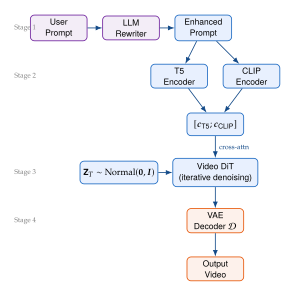
System-Level Considerations
We briefly discuss design choices made by three influential T2V systems.
Sora.
OpenAI's Sora [6] frames video generation as “world simulation,” emphasising that the model should learn physical laws, object permanence, and 3D consistency from data alone, without explicit physics engines. Sora uses a spacetime patches approach, processing the video as a sequence of 3D patches that are fed to a DiT. The prompt enhancement step (using GPT-4) is a critical component, transforming user queries into detailed scene descriptions that guide the model's internal world simulation.
CogVideoX.
CogVideoX [17] introduces an “expert transformer” architecture. The name suggests two networks, but the mechanism is subtler and cheaper to describe than that: text tokens and video tokens live in one sequence and are processed by one full 3D attention, and what is duplicated per modality is only the adaptive layer-normalisation and the associated projections - separate scale and shift parameters for text tokens and for video tokens, both modulated by the diffusion timestep. The motivation is a numerical one: text embeddings from a frozen T5 and video latents from a 3D VAE have very different scales and distributions, and forcing them through shared normalisation statistics degrades the fusion.
It is worth being explicit that this design does not reduce attention cost. Attention runs over the concatenated sequence, so it remains quadratic in the combined text-plus-video length; the expert parameters buy alignment quality, not efficiency. The efficiency argument in CogVideoX is made elsewhere - in the 3D VAE's temporal compression and in progressive training that starts with short, low-resolution clips and grows duration and resolution over the schedule.
Movie Gen.
Movie Gen [32] is designed as a “cast of foundation models,” where different components (video generation, audio generation, editing) are implemented as separate models that share a common architecture and training paradigm. The video generation component uses a 30B-parameter transformer trained on a mixture of image and video data, with the data mixing ratio carefully tuned to balance per-frame quality against temporal coherence.
Key Idea.
The complete T2V system is more than the diffusion model. While the diffusion model is the core generative engine, the overall quality of a T2V system depends critically on auxiliary components: the prompt rewriter (which determines the quality of the conditioning signal), the text encoders (which determine how faithfully the conditioning is represented), the VAE (which determines the ceiling of visual quality), and the post-processing pipeline (which handles upsampling and artefact correction). Improving any of these components can yield quality gains comparable to improving the diffusion model itself.
Exercise 37 (Prompt enhancement evaluation).
Design an experiment to measure the effectiveness of prompt enhancement. Given a set of user prompts, generate videos using both the original prompts and LLM-enhanced prompts. Propose at least three evaluation metrics (both automated and human) and discuss potential confounds (e.g., the enhanced prompt may be “better” not because of additional detail but because it aligns more closely with the training data distribution).
Exercise 38 (T5 vs. CLIP encoding).
Consider a video diffusion model trained with dual T5+CLIP encoding. Describe an ablation experiment to measure the contribution of each encoder. What do you expect to happen when you: (a) replace the T5 embedding with zeros (CLIP-only)? (b) replace the CLIP embedding with zeros (T5-only)? (c) use two copies of the same encoder? Relate your predictions to the different training data and objectives of T5 and CLIP.
Personalisation and Adaptation
A pre-trained video diffusion model captures the distribution of generic videos seen during training. For many applications, however, we want to generate videos featuring specific subjects (a particular person, pet, product, or scene), specific visual styles (anime, watercolour, cinematic noir), or specific motion patterns (a characteristic dance move, a recurring camera technique). Personalisation adapts a pre-trained model to these specific requirements using a small amount of reference data, typically a few images or short video clips.
The central challenge is efficiency: a state-of-the-art video diffusion model may have 5–30 billion parameters. Full fine-tuning on a few reference examples is (i) computationally expensive, (ii) prone to catastrophic forgetting of the model's general capabilities, and (iii) prone to overfitting to the small reference set. Low-rank adaptation (LoRA) addresses all three issues by restricting the parameter update to a low-dimensional subspace.
Low-Rank Adaptation (LoRA)
Definition 68 (Low-Rank Adaptation).
Let be a pre-trained weight matrix in the diffusion model (e.g., a linear projection in an attention layer). Low-Rank Adaptation (LoRA) [40] replaces with (LORA) where
is the down-projection, mapping the input into an -dimensional bottleneck, and
is the up-projection, mapping that bottleneck back to the output space,
with rank . The pre-trained weight is frozen; only and are updated during fine-tuning. We follow the factor ordering of [40] throughout, so that always denotes the down-projection and the up-projection; the transposed convention also appears in the literature and the two differ only in naming.
The key insight is that the weight update is constrained to the set of rank- matrices. If the task-specific adaptation requires changes that are approximately low-rank (which empirical evidence strongly suggests), LoRA can capture these changes with far fewer parameters than full fine-tuning.
Proposition 36 (LoRA Parameter Count).
For a video DiT with attention layers, each containing linear projections of dimension , the total number of LoRA parameters is (LORA Param Count) where the factor accounts for both and . For a typical configuration (, , projections per layer for , , , and output, layers), this gives (LORA Param Example) which is roughly – of the total parameters in a 5B–15B parameter model.
Remark 74 (LoRA initialisation).
Following [40], the down-projection is initialised from a random Gaussian and the up-projection is initialised to zero, so that at the start of training. The adapted model therefore begins as an exact copy of the pre-trained model - the same “start as a no-op” principle as ControlNet's zero convolutions (Video ControlNet) and adaLN-Zero.
The reason for zeroing exactly one factor rather than both is worth spelling out, because it is easy to state wrongly. It is not that the asymmetry breaks some symmetry between the rows and columns of : the mirror-image choice (, Gaussian) is the same scheme up to transposition and would work equally well. The real reason is that zeroing exactly one factor is the only way to get both properties at once:
The product starts at zero, so no pre-trained behaviour is perturbed at step , and the fine-tuning run begins from a known-good model rather than from a randomly displaced one.
The gradient does not start at zero. By the product rule, , which is generically non-zero precisely because is not zero. The adapter is a no-op in the forward pass while still receiving gradient in the backward pass.
Zeroing both factors would satisfy (i) and destroy (ii): and would both vanish and the adapter would never leave the origin. Initialising neither to zero would satisfy (ii) and destroy (i).
Approximation Quality of LoRA
How well can a rank- update approximate the optimal full-rank adaptation? The following proposition provides a bound.
Proposition 37 (Rank-Constrained Adaptation Bound).
Let be the optimal weight matrix obtained by full fine-tuning, and let be the LoRA-adapted weight with rank . The optimal rank- approximation to the full update satisfies (LORA Eckart Young) where are the singular values of in decreasing order. In particular, if (i.e., the optimal update is exactly rank ), then LoRA achieves zero approximation error.
Proof.
This is a direct application of the Eckart–Young–Mirsky theorem. The optimal rank- approximation to any matrix in the Frobenius norm is obtained by truncating its singular value decomposition to the top singular values. Setting and noting that is rank at most , the result follows.
Insight.
LoRA works because adaptations are approximately low-rank. The premise on which the whole method rests is that has a rapidly decaying singular value spectrum, so that the tail sum in (LORA Eckart Young) is small at modest . This is an empirical claim about fine-tuning, not a theorem, and it is one you can check directly for your own model: run a short full fine-tune, take the SVD of for a few attention projections, and plot the cumulative energy against . The diagnostic in Practical Considerations is the same measurement made after the fact on the learned adapter. Where the premise holds, a small costs almost nothing relative to full fine-tuning; where it fails - and it does fail for adaptations that genuinely change the model's behaviour broadly rather than adding one subject or style - LoRA will silently underfit, and the singular value plot is how you find out.
This low-rank structure arises because personalisation typically requires changes to a small number of “directions” in weight space: the model needs to learn a new face, a new style, or a new motion pattern, each of which corresponds to a low-dimensional subspace of the full parameter space.
LoRA for Video DiT
Applying LoRA to a video diffusion transformer requires choosing which layers to adapt and with what rank. The design space includes:
Spatial attention: Adapting the spatial self-attention projections (, , , output) changes the model's visual features: how it represents textures, shapes, and object appearances. This is the most important target for subject personalisation (learning a specific face or object).
Temporal attention: Adapting the temporal self-attention projections changes the model's motion dynamics: how objects move, how scenes evolve, and what temporal patterns are generated. This is the primary target for motion personalisation (learning a specific dance move or camera technique).
Cross-attention: Adapting the cross-attention projections (where text embeddings interact with visual features) changes the model's text-visual alignment: how it maps words to visual concepts. This is useful for learning new vocabulary (associating a trigger word with a specific subject or style).
Feed-forward layers: Adapting the MLP layers changes the model's non-linear feature transformations. This is less commonly targeted by LoRA in video diffusion but can be useful for style adaptation.
Example 47 (AnimateDiff: Motion LoRA).
Guo et al. [37] demonstrate a compelling application of LoRA for video personalisation. Starting from a pre-trained text-to-image model, they insert temporal attention layers (a “motion module”) and train them on video data while keeping the spatial layers frozen. The motion module can be viewed as a LoRA-like adapter that adds temporal capabilities to an image-only model.
Once trained, different motion modules can be swapped in and out to change the motion style without affecting the visual style. Furthermore, the motion module can be combined with any personalised text-to-image model (e.g., a DreamBooth model of a specific person), enabling the generation of personalised videos with custom motion patterns. This factorisation of visual appearance and motion dynamics is a powerful design principle.
DreamBooth for Video
DreamBooth [70] fine-tunes a diffusion model on a small set of images (3–5) of a specific subject, associating it with a unique identifier token (e.g., “a photo of [V] dog”). The key insight is the prior preservation loss, which ensures that the model retains its general capabilities while learning the new subject.
Definition 69 (DreamBooth Loss for Video).
Let be a small set of reference videos (or images) of the target subject, and let be the corresponding prompts with the unique identifier token [V]. The DreamBooth loss for video is (Dreambooth LOSS) where is a class-level prompt (without the identifier token), is the distribution of class-level videos generated by the pre-trained model, and controls the strength of prior preservation.
The prior preservation term prevents the model from “forgetting” the general concept of “dog” while it learns the specific appearance of the subject. Without it, the model would collapse: all dogs would look like the specific subject, and the trigger token “[V]” would become synonymous with the class label.
Remark 75 (DreamBooth + LoRA).
In practice, DreamBooth for video is almost always combined with LoRA rather than full fine-tuning. This combination offers the best of both worlds: DreamBooth's ability to learn new subjects from a few examples, and LoRA's parameter efficiency and resistance to overfitting. The resulting “DreamBooth-LoRA” adapters are small files (typically 10–100 MB) that can be shared, swapped, and composed.
Composing Adapters
A powerful feature of LoRA-based personalisation is the ability to compose multiple adapters. If adapter 1 contributes and adapter 2 contributes , the composed model uses (LORA Compose) where are blending weights. This allows, for example, combining a subject adapter (to generate a specific person) with a style adapter (to render in a specific artistic style) and a motion adapter (to specify a particular motion pattern).
Caution.
Adapter composition is not guaranteed to work. The additivity assumption in (LORA Compose) is a linear approximation. When the two adapters modify overlapping subspaces of the weight matrix, their effects can interfere destructively. Empirically, composition works well when the adapters target different aspects of the model (e.g., spatial attention for appearance and temporal attention for motion) but can produce artefacts when both adapters modify the same layers. Reducing the blending weights mitigates interference at the cost of weaker adaptation effects.
Proposition 38 (Rank of Composed Adapters).
Let and let the individual adapters have ranks and . The composed weight update satisfies . If in addition
the column spaces of and intersect only in , and
the stacked down-projection has full row rank ,
then the rank is exactly . If either condition fails, the rank may be strictly lower.
Proof.
Write with and . The inner dimension is , giving the upper bound. Condition (i) makes injective on , so , and condition (ii) makes that .
Remark 76 (Why both conditions are needed).
Orthogonality of the up-projections alone is not enough, and the counterexample is not exotic: take , so that both adapters read the same -dimensional subspace of the input and merely write it to different places. Then has rank , not , and has rank at most however orthogonal and are. Condition (ii) is generic - two independently trained adapters will satisfy it almost surely - but “generic” is not “always”, and adapters trained on related data from the same base model are exactly the case where it is least safe to assume. This is the algebraic shadow of the interference warning above: rank deficiency in the composition is what destructive interference looks like when you count dimensions.
Quantised LoRA (QLoRA)
For very large video diffusion models, even loading the pre-trained weights into GPU memory can be challenging. QLoRA [71] addresses this by quantising the frozen base weights to 4-bit precision while keeping the LoRA adapter weights in full precision (16-bit or 32-bit).
Definition 70 (Quantised LoRA).
Let be the pre-trained weight matrix. QLoRA replaces the forward pass with (Qlora) where is the 4-bit quantised version of , restores it to the computation dtype (BFloat16), and are the full-precision LoRA matrices. The quantisation error is partially compensated by the LoRA update during fine-tuning.
Example 48 (Memory savings with QLoRA).
Consider a 15B-parameter video DiT:
| Method | Base Model Memory | Total Memory |
| Full fine-tuning (FP16) | 30 GB | 90+ GB |
| LoRA (FP16 base) | 30 GB | 31 GB |
| QLoRA (4-bit base) | 7.5 GB | 8.5 GB |
Practical Considerations
We conclude with practical guidelines for personalising video diffusion models.
Rank selection: The rank controls the trade-off between expressiveness and efficiency. For subject personalisation, – is typical; for style transfer, – often suffices; for complex motion patterns, – may be needed. A useful diagnostic is to plot the singular value spectrum of the learned after training: if the smallest singular values are near zero, the rank is too high (wasting parameters); if they are large, the rank may be too low.
Learning rate: LoRA fine-tuning typically uses learning rates to higher than full fine-tuning because the gradient signal must be “concentrated” into a much smaller parameter subspace. Common values are to for LoRA versus to for full fine-tuning.
Training duration: Overfitting is the primary risk when personalising on a small dataset. For subject personalisation with 3–5 reference images, 500–2000 training steps are typical. For motion personalisation from short video clips, 1000–5000 steps are common. Early stopping based on a held-out validation metric (e.g., CLIP similarity to the reference) is recommended.
Regularisation: Beyond the DreamBooth prior preservation loss, additional regularisation strategies include: itemize
Weight decay on the LoRA parameters.
Gradient clipping to prevent sudden large updates.
Augmenting the reference data with random crops, colour jitter, and temporal shifts. itemize
Which layers to adapt: Not all layers contribute equally to personalisation. Attention projections in the middle layers of the transformer are most important for both subject and style adaptation; early and late layers contribute less. Adapting only the middle of layers can reduce the adapter size by half with minimal quality loss.
Algorithm 6 (LoRA Fine-Tuning for Video Personalisation).
Input: Pre-trained video DiT , reference data , rank , learning rate , training steps .
Initialise: For each target layer , create and .
For : enumerate[(a)]
Sample a reference example and noise , .
Encode: .
Noise: .
Predict: using for adapted layers.
Loss: .
Update: (only LoRA parameters). enumerate
Output: Adapter weights .
Summary and Forward Pointers
This section has covered the core techniques for adapting pre-trained video diffusion models to specific subjects, styles, and motion patterns. LoRA provides a parameter-efficient mechanism for adaptation, with theoretical guarantees on approximation quality (Proposition 37) and practical recipes for rank selection, learning rate tuning, and regularisation. DreamBooth extends the paradigm to subject-driven generation with prior preservation. Adapter composition enables combining multiple adaptations without retraining.
Everything in the last five sections has taken the model's native generation window for granted: a clip of a few seconds, generated in one shot, and then controlled. The next chapter of the story drops that assumption. Long Video Generation confronts the fact that these models generate two to ten seconds while users want minutes, and works through the two ways out - autoregressive chunking, which accumulates drift, and hierarchical keyframe generation, which trades that drift for a planning problem. Temporal Consistency and Coherence then asks what temporal consistency even means quantitatively, and what an attention window of finite size can and cannot guarantee about it. Video Editing turns from generation to editing an existing video, where the control problem reappears in a sharper form: the output must change in one respect and stay identical in every other. Physics-Aware Video Generation and World Models closes with the question the whole field is circling - whether a model that predicts video frames has thereby learned anything about the world that produced them - and Autoregressive-Diffusion Hybrids with the autoregressive and diffusion paradigms converging on each other.
The connection to the present section is direct. Personalisation and control are how you steer a single short clip; long-horizon generation is where those same steering signals must be kept consistent across many clips, and consistency is precisely what degrades first.
Exercise 39 (LoRA rank analysis).
Train a LoRA adapter for a video diffusion model at ranks . For each rank, compute: (a) the training loss, (b) the FVD (Fréchet Video Distance) of generated samples, (c) the CLIP similarity to the reference subject. Plot all three metrics as a function of . At what rank does performance plateau? How does this relate to the singular value spectrum of the learned ?
Exercise 40 (Temporal vs. spatial LoRA).
Design an experiment to compare adapting only spatial attention layers versus only temporal attention layers versus both. Use a character animation task (given reference images of a person, generate video of them performing a specific action). Predict which configuration will produce: (a) the best identity preservation, (b) the best motion quality, (c) the best overall video quality. Justify your predictions using the analysis of spatial versus temporal attention from earlier sections.
Exercise 41 (Adapter interference).
Given two independently trained LoRA adapters and , define a measure of “interference” between them. One candidate is , the cosine similarity between the vectorised weight updates. Another is the overlap between the column spaces of the up-projections and (see Proposition 38). Discuss the pros and cons of each measure. How would you use such a measure to predict whether two adapters will compose well?
Long Video Generation
The video diffusion models we have studied so far generate clips of fixed, modest duration: typically 2 to 10 seconds, corresponding to 16 to 240 frames depending on the frame rate. This window is dictated by the model's temporal attention span and by the memory required to process the full latent tensor during training. Yet the videos people actually want to create, a product demonstration, a short film, a gameplay walkthrough, span minutes or hours. Bridging the gap between a model's native generation window and the durations demanded by real applications is one of the central open problems in video generation.
The difficulty is not merely computational. Even if we had unlimited memory, training a single model on very long sequences would require prohibitively large datasets of consistently annotated long videos, and the quadratic cost of attention over hundreds or thousands of frames would dominate the compute budget. Instead, the field has developed a family of strategies that compose short-window models to produce long outputs while maintaining temporal coherence across chunk boundaries. We examine the two principal paradigms: autoregressive chunk generation and hierarchical keyframe generation.
The fundamental tension
Let us formalise the problem. Suppose our diffusion model can generate video chunks of frames each. We wish to produce a video of frames. The model's learned distribution captures statistics of -frame sequences, but says nothing directly about the joint distribution over the full video. Any long-generation strategy must therefore make assumptions about how to factorise or approximate using the model's native capacity.
Key Idea.
Short models, long videos. The core challenge of long video generation is to use a model trained on -frame windows to produce -frame videos with , while maintaining global coherence that the model was never explicitly trained to enforce. Every strategy for achieving this involves a trade-off between computational cost, temporal consistency, and generation diversity.
Two broad failure modes characterise long video generation. The first is drift: the video's content gradually shifts away from its initial state, so that characters change appearance, scenes morph imperceptibly, and the visual style wanders. The second is repetition: the model falls into a low-energy attractor and produces the same motion pattern in a loop, typically a subtle rocking or breathing motion with no narrative progression. Good long-generation methods must combat both simultaneously.
Autoregressive chunk generation
The most natural approach to long video generation is to produce the video one chunk at a time, conditioning each new chunk on the tail of the previous one. This mirrors the autoregressive structure of language models, where each token is generated conditioned on all preceding tokens.
Definition 71 (Autoregressive Chunk Generation).
Let denote the -th chunk of a long video, where each chunk has frames. Let be the overlap parameter specifying how many frames from the end of chunk are used to condition chunk . The autoregressive chunk generation factorisation is (AR Chunk) where denotes the last frames of chunk , and is the total number of chunks needed to cover frames.
In practice, the conditioning is implemented by one of several mechanisms.
Latent initialisation. Encode the conditioning frames into the latent space and concatenate or replace the corresponding positions in the noisy latent tensor before denoising begins. The denoising process then “paints in” only the new frames while respecting the boundary.
Cross-attention conditioning. Feed the conditioning frames (or their features) as additional keys and values to the temporal cross-attention layers. This gives the model soft access to the context without hard-copying any frames.
Noise blending. During the reverse diffusion process, maintain a “clean” copy of the overlap region and blend it with the denoised prediction at each step, using a schedule that transitions smoothly from noisy to clean. This avoids hard boundaries.
Remark 77 (Choosing the overlap ).
The overlap trades off redundancy against coherence. A small (e.g., 1 or 2 frames) minimises redundant computation but provides the model with very little context about the previous chunk, making drift likely. A large (e.g., ) gives the model extensive context but doubles the effective cost per output frame. In practice, values of frames offer a good balance, corresponding to roughly 0.1 to 0.5 seconds of context at 30 fps.
The critical question is: how do errors behave as we chain more chunks? The question has to be posed carefully, because the obvious formulation is vacuous. The deviation of the generated video from a reference video is a concatenation of the per-chunk deviations along the time axis, not a sum of vectors: if every chunk satisfies then (Error Concatenation) holds deterministically, with no independence assumption, no zero-mean assumption and no cross terms to cancel. Worse, this bound is insensitive to the very thing we care about: it is the same whether the chunks were generated independently or chained, because it never models the fact that chunk is conditioned on chunk 's already-corrupted output.
What actually degrades over a long autoregressive rollout is not the per-frame reconstruction error but the cumulative displacement of the video's slowly varying content: a character's face, the colour palette, the lighting direction, the camera's implicit position. Each chunk inherits the previous chunk's version of that content and adds its own small increment, and the increments never get undone. The object to bound is therefore the running sum of those increments, and the following statement makes that model explicit.
Proposition 39 (Drift Accumulation in Autoregressive Chunking).
Let be a vector summarising the slowly varying content of chunk (appearance, palette, identity, implicit camera pose), and let be its intended value. Assume:
Inheritance. Chunk sees the past only through the tail of chunk , so that , where is the increment contributed by the -th generation step.
Bounded increment. for every .
No restoring force. Nothing in the pipeline pulls back towards ; the only reference available to chunk is chunk .
Write for the drift after chunks. Then:
Correlated increments (systematic bias). (Error Worst) with equality precisely when every increment has magnitude and all point in the same direction. Drift then grows linearly in the chunk count.
Decorrelated increments. If in addition the increments are zero-mean and pairwise uncorrelated, with , then (Error Independent) so the root-mean-square drift grows only as .
Proof.
Part (a) is the triangle inequality, , and the equality case is the equality case of the triangle inequality: the sum of norms is attained only when all summands are non-negative multiples of a common unit vector, and additionally requires for all . For part (b), expand the squared norm: where the cross terms vanish because the increments are zero-mean and uncorrelated.
Caution.
Assumptions (A1)–(A3) are a model of autoregressive chunking, not a consequence of it, and (A2) in particular hides the real failure mode. If the conditioning is corrupted, the next increment is typically larger, not merely another draw of size ; a Lipschitz model gives , which is exponential whenever . Proposition 39 should therefore be read as describing the best case one can hope for, not a guarantee.
Insight.
The linear-versus-square-root distinction in Proposition 39 has direct practical consequences. For a 2-minute video at 24 fps generated as non-overlapping 16-frame chunks, . If each chunk nudges the appearance in a consistent direction (say, every chunk warms the colour temperature slightly), the drift after two minutes is ; if the nudges are decorrelated, it is only . The difference is more than an order of magnitude, and it explains why the two practical remedies are (i) designing chunk transitions so that successive increments do not share a systematic bias, and (ii) violating assumption (A3) outright by supplying a fixed, chunk-independent reference that pulls the state back towards . Replacing (A1) with a contraction for some bounds the drift by for every : the anchoring mechanism of the next example is exactly such a restoring force.
Example 49 (StreamingT2V).
StreamingT2V [41] implements autoregressive chunk generation with two conditioning pathways of different range. A short-range conditional attention module attends to the last few frames of the previous chunk and handles smooth continuation across the boundary. A long-range appearance preservation module extracts high-level scene and object features from a fixed anchor frame taken from the very first chunk; these features are mixed into the prompt embedding and injected through the spatial cross-attention layers.
The anchor is deliberately not refreshed. Because it never changes, the global appearance reference is the same for every chunk in the rollout, which is precisely the restoring force of assumption (A3) in Proposition 39: refreshing the anchor from a recent frame would make the reference itself drift and would defeat the module's purpose.
Example 50 (FreeNoise).
FreeNoise [42] takes a different approach to long video generation by operating on the noise schedule rather than the conditioning mechanism. Instead of generating chunks independently and stitching them, FreeNoise constructs a temporally correlated noise sequence for the entire long video. The key insight is that if adjacent chunks share their initial noise in the overlap region, the denoised outputs will naturally align without explicit conditioning. Concretely, for chunks and , the initial noise tensors satisfy , where the subscripts index the temporal positions within each chunk. This simple modification, requiring no architectural changes or additional training, significantly reduces boundary artifacts.
Hierarchical keyframe generation
Autoregressive methods process the video strictly left-to-right, which means that early decisions irreversibly constrain later content. An alternative paradigm first generates a sparse set of keyframes that establish the global structure, then fills in the gaps through interpolation. This “coarse-to-fine” strategy mirrors how human animators work: first sketch the key poses, then draw the in-between frames.
Definition 72 (Hierarchical Keyframe Generation).
A hierarchical keyframe generation procedure operates in levels. At level (the coarsest), a diffusion model generates keyframes spaced frames apart: (Keyframe Level0) At each subsequent level , an interpolation model generates intermediate frames conditioned on the keyframes from level : (Keyframe Interp) where is the temporal upsampling factor at level . The final video is with (every frame present).
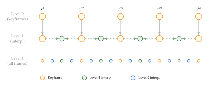
The hierarchical approach offers several advantages over purely autoregressive generation.
Global coherence. Because the keyframes are generated jointly (or with global conditioning), they establish a consistent narrative arc that the interpolation stages must respect. This reduces drift.
Parallelism. The interpolation between two keyframes is independent of the interpolation between two other keyframes. This enables embarrassingly parallel generation at each level, dramatically reducing wall-clock time.
Error isolation. An error in one interpolation segment does not propagate to distant segments, because the keyframes anchor both endpoints. This limits error accumulation to within-segment drift.
Proposition 40 (Optimal Keyframe Spacing).
Consider a scene with characteristic motion signal-to-noise ratio , defined as the ratio of the coherent (predictable) component of the optical flow field to the standard deviation of the residual left after fitting a smooth motion model, i.e. of the part of the motion that an interpolator cannot anticipate. High therefore means predictable motion, not necessarily slow motion. The optimal keyframe spacing that minimises total reconstruction error (balancing keyframe generation error and interpolation error) satisfies (Optimal Spacing)
Proof sketch.
Let denote the error per keyframe when generating keyframes spaced apart. A wider spacing means fewer keyframes to generate, reducing the number of difficult generation steps, so decreases with (fewer, simpler decisions). Let denote the interpolation error for a gap of frames. When the motion is well predicted by a smooth model (high ), interpolation is easy; when a large fraction of the motion is unpredictable (low ), interpolation degrades. Under standard assumptions about optical flow prediction accuracy, .
The total number of keyframes is , and the total number of interpolation segments is also . The total error is approximately Treating as roughly constant (its dependence on is weak) and substituting the linear model for , we get . Minimising over gives .
Remark 78 (Interpreting optimal spacing).
Proposition 40 formalises an intuition that animators have long understood: for coherent, predictable motion (high , such as a steady dolly shot or a talking head), wide keyframe spacing is fine because interpolation is easy. For erratic, hard-to-anticipate motion (low , such as a fight scene or splashing water), keyframes must be closely spaced to prevent interpolation artifacts. Note that the relevant axis is predictability rather than speed: a fast but rigid camera pan can have a higher than slow, turbulent smoke. Adaptive keyframe placement, where the spacing varies across the video based on local motion complexity, is a natural extension.
Example 51 (NUWA-XL).
NUWA-XL [43] implements a particularly elegant form of hierarchical generation. The architecture uses a “diffusion over diffusion” design in which a global diffusion model generates keyframes spanning the whole time range from prompts, and local diffusion models then recursively fill in the frames between adjacent keyframes, each local model taking its two bracketing keyframes as first-frame and last-frame visual conditions.
The unifying element is a single backbone design, Mask Temporal Diffusion, which accepts visual conditions with or without the first and last frames: the global stage runs it with an all-zero visual condition, the local stages run it with the bracketing frames supplied. The two stages therefore share an architecture; they are trained and applied as separate stages of a coarse-to-fine pipeline, not as one end-to-end network. Because every segment at a given level is conditioned only on its own two endpoints, all segments at that level can be generated in parallel: a scheme of depth with local length covers frames. NUWA-XL was trained directly on 3,376-frame videos, and on 1,024-frame generation it reduced inference time by roughly relative to sequential generation. Maintaining fine-grained consistency over such durations nevertheless remains challenging.
The hierarchical approach can be analysed as a tree-structured computation, where the root generates global structure and the leaves produce individual frames. This tree structure enables a clean complexity analysis.
Proposition 41 (Complexity of Hierarchical Generation).
Consider an -level hierarchical generation scheme where level upsamples the frame rate by factor . If each diffusion generation call takes time (independent of temporal length, up to the model's native window), then:
The total number of diffusion calls is (HIER CALL Count) a sum dominated by its last term, since decreases with .
With parallelism at each level, the wall-clock time is , independent of .
The total drift is bounded by , where is the per-level error - a sum of terms, compared with a drift of up to for autoregressive generation with chunks (Proposition 39).
Proof sketch.
Level generates the keyframes directly. For , the frames present after level are spaced apart, so there are gaps to fill, each requiring one interpolation call. This count grows with (the finest level does the most work), so the sum is a geometric series dominated by its last term and is . Since all segments at a given level are conditioned only on their own two endpoints, they are independent and can be processed in parallel, reducing the depth to . The error bound follows from the triangle inequality applied across the levels rather than across the chunks.
Remark 79 (Hierarchical vs. autoregressive: a quantitative comparison).
For a 1-minute video at 24 fps ( frames), consider:
Autoregressive with , : sequential chunk generations, with worst-case drift .
Hierarchical with levels and upsampling factors , hence and keyframes: sequential stages with full parallelism within each stage, and error bound .
The hierarchical approach is faster in wall-clock time (assuming unlimited parallelism) and has dramatically better error bounds, at the cost of requiring more total compute (all parallel segments must be processed) and more complex orchestration.
Temporal noise schedules for long generation
A subtle but important consideration in autoregressive chunk generation is the design of the noise schedule at chunk boundaries. When the model begins denoising a new chunk, the overlap region contains “clean” frames from the previous chunk, while the remaining positions are pure noise. This mismatch between clean and noisy regions can cause artifacts.
Definition 73 (Temporal Noise Ramp).
A temporal noise ramp is a position-dependent noise schedule for chunk , where the noise level at frame position within the chunk depends on its distance from the overlap boundary: (Noise RAMP) where is the width of the transition zone and is the base noise level at diffusion step . (The subscript distinguishes it from the attention window of Attention window and consistency guarantees.)
The noise ramp ensures a smooth transition from the clean context to the fully noisy region, avoiding the hard boundary that would otherwise cause visible seams.
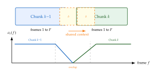
Combining strategies: the hybrid approach
The autoregressive and hierarchical approaches are not mutually exclusive. In fact, the most effective long video generation systems combine both.
Algorithm 7 (Hybrid Long Video Generation).
Plan: Use a language model or planning module to decompose the target video into semantic segments, each with a text description .
Keyframe generation: Generate one keyframe per segment using an image diffusion model, conditioned on and (optionally) the previous keyframe: .
Segment interpolation: For each pair of adjacent keyframes , generate the in-between frames using a video interpolation diffusion model: .
Temporal super-resolution: Optionally increase the frame rate through temporal upsampling.
This hybrid approach inherits the global coherence of hierarchical generation (through planned keyframes) and the local quality of autoregressive generation (through segment-level diffusion).
Caution.
Long video generation remains an active research frontier. Even the best current systems exhibit drift over durations exceeding 30 seconds, struggle with complex multi-character narratives, and produce noticeable boundary artifacts at chunk transitions. The drift accumulation model of Proposition 39 is not a merely theoretical concern; the linear regime it describes is what a viewer sees as a character's face slowly becoming a different face.
The long-range consistency challenges of video generation connect deeply to the memory architectures studied in 24. The fundamental question of how to maintain coherent state over extended sequences arises in both language modelling and video generation, and solutions from one domain often inspire progress in the other. Similarly, the problem of generating consistent content over long durations relates to the continual learning challenges discussed in 26, where models must maintain stable representations while adapting to new inputs.
Exercise 42 (Analysing chunk boundaries).
Consider autoregressive chunk generation with frames per chunk, overlap , and a target video of frames.
How many chunks are needed?
What fraction of the total computation is “wasted” on re-generating overlap frames?
Explain why the PSNR of the concatenated video is essentially the average of the per-chunk PSNRs, and so says nothing about drift. (Hint: compare (Error Concatenation) with (Error Worst).)
Using the drift model of Proposition 39 with a per-chunk increment of magnitude , give the drift at the final chunk under (i) systematically aligned increments and (ii) zero-mean uncorrelated increments.
Propose a modification to the noise ramp (Definition 73) that uses a cosine transition instead of a linear one. What advantage might this offer?
Exercise 43 (Hierarchical generation tree).
Consider a 3-level hierarchical generation scheme (Definition 72) targeting frames. Level 0 generates keyframes at spacing ; level 1 refines the spacing to ; level 2 refines it to .
What are the temporal upsampling factors and ? How many frames are present after each level? (Note that a 3-level scheme has only two interpolation steps, and hence only two upsampling factors.)
Draw the generation tree, showing which frames are generated at each level.
If each interpolation call fills exactly the frames lying strictly between two consecutive frames of the previous level, how many calls are needed at each level? What is the maximum parallelism?
Compare the wall-clock time to autoregressive generation with 16-frame chunks and 4-frame overlap, assuming each model call takes 10 seconds.
Temporal Consistency and Coherence
A beautiful video that flickers, wobbles, or allows characters to subtly morph between frames is not a good video. Temporal consistency, the property that corresponding regions across frames depict the same content in a physically plausible manner, is arguably the single most important quality criterion for generated video. Human viewers are extraordinarily sensitive to temporal inconsistencies: a shadow that shifts by a few pixels, a texture that shimmers, or an expression that momentarily changes can render an otherwise photorealistic video immediately unconvincing.
In this section, we formalise what temporal consistency means, present quantitative metrics for measuring it, and study how architectural choices in diffusion models affect the degree of consistency achievable.
Measuring temporal consistency
Intuitively, temporal consistency means that if we warp frame back to the coordinate system of frame using the true optical flow, the result should match frame closely. This leads to the following formal definition.
Definition 74 (Temporal Consistency Score).
Let be a video, let be a perceptual feature extractor (e.g., a pre-trained network), and let denote the optical flow field from frame to frame . The temporal consistency score is (TC Score) where denotes backward warping of image according to flow field , and is a similarity function (e.g., cosine similarity in feature space).
Remark 80 (Why perceptual features?).
Computing TC in pixel space (i.e., setting to the identity) is problematic because optical flow estimation introduces sub-pixel errors, and bilinear warping causes slight blurring. These artifacts reduce pixel-level similarity even for perfectly consistent videos. Perceptual features from networks like VGG or DINO are more robust to these small spatial perturbations, giving a cleaner signal about actual temporal inconsistency versus measurement noise.
A caution on terminology: the abbreviation “TC” is also used in the evaluation literature for a different quantity, the CLIP-based score of Definition 86, which compares raw adjacent-frame embeddings with no warping at all. Definition 74 is a flow-warped perceptual similarity and is the notion used throughout this section; the two are not interchangeable and should not be compared numerically.
While TC measures frame-to-frame smoothness, many applications require a stronger form of consistency: that specific entities maintain their identity throughout the video.
Definition 75 (Identity Consistency).
Let be a video containing one or more identifiable entities (e.g., faces, specific objects). Let denote the embedding of the detected face (or entity) in frame , extracted by a recognition network. The identity consistency score is (Identity Consistency) where the minimum is taken over all pairs of frames in which the entity is visible.
Remark 81 (Minimum versus average).
Definition 75 uses the minimum similarity rather than the average. This is deliberate: a video where a character's face is consistent in 99 out of 100 frames but grotesquely distorted in one frame is not a good video. The worst-case formulation captures this; an average would hide it. In practice, one often reports both the minimum and the mean, but the minimum is the binding constraint.
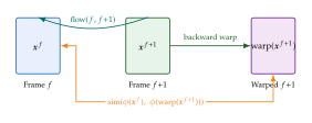
Attention window and consistency guarantees
A video diffusion model's temporal attention mechanism is the primary tool by which it enforces consistency across frames. If the model uses full temporal attention (every frame attends to every other frame), then the model can, in principle, detect and correct inconsistencies between any pair of frames. In practice, memory constraints often force the use of windowed or sparse attention, where each frame attends only to a local neighbourhood. Beyond the window, consistency between two frames is not enforced directly: it has to be relayed through a chain of intermediate frames, and the relay is lossy. The following result quantifies how lossy, under assumptions that must be stated explicitly because they, and not the attention mechanism, are what does the work.
Proposition 42 (Chain Relay of Consistency Beyond the Window).
Let a video diffusion model use temporal self-attention with window size (each frame attends to the nearest frames in both directions). Assume:
Metric features. The perceptual features are unit-norm, and the consistency between two frames is the cosine similarity of their features after warping to a common coordinate frame, so that the inconsistency , where denotes the warped feature.
In-window guarantee. whenever .
Composable warps. Warping through an intermediate frame agrees with warping directly, so the chain introduces no warping error of its own.
Write for the consistency of a frame pair at separation , and for let be the number of hops in the shortest relay chain. Then (Consistency Degradation) and if the per-hop feature displacements are in addition zero-mean and pairwise uncorrelated, (Consistency Degradation Indep) For the pair lies inside the window and (H2) applies directly: .
Proof.
Write , a genuine metric, so by (H1) and (H2) reads within the window. Let be a chain whose consecutive frames are at most apart; by (H3) the warped features may all be compared in one coordinate frame.
For the first bound, the triangle inequality gives , whence . This is tight when every hop displaces the feature in the same direction, i.e. when the model has a systematic bias.
For the second bound, decompose with and . If the are zero-mean and pairwise uncorrelated the cross terms vanish, so and .
Caution.
Proposition 42 is a bound on a model of the relay, not a property of attention. Its hypotheses are strong - (H3) in particular is false whenever optical flow is imperfect, which is always - and both bounds are vacuous once the right-hand side falls below the similarity of two unrelated frames. With and the aligned bound expires at hops ( frames, under 5 s at 24 fps) and the decorrelated bound at hops ( frames, about 33 s). Nothing here proves that consistency degrades; what the proposition supplies is a range of horizons over which one could still certify it, and the empirically observed drift horizon of current systems sits inside that range.
Insight.
The useful content of Proposition 42 is the shape of the degradation, and it mirrors Proposition 39 exactly. Doubling the video length while holding the window fixed doubles the hop count , which doubles the guaranteed inconsistency if the per-hop errors are decorrelated and quadruples it if they share a systematic bias. Consistency is therefore bought in two ways: enlarging (fewer hops for the same separation), or removing hops altogether. The latter is what hierarchical generation (Hierarchical keyframe generation) does - keyframes are mutually in-window at level 0, so every later frame is only a couple of hops from a global anchor rather than hops from its distant neighbour - and it is also what a fixed anchor frame does in the autoregressive setting.
Methods for improving temporal consistency
Given the fundamental limitations imposed by finite attention windows, researchers have developed several techniques to improve temporal consistency beyond what the base model provides.
Example 52 (FreeInit).
FreeInit [44] observes that the initial noise used to start the denoising process has a significant impact on temporal consistency. Specifically, if the low-frequency components of the initial noise are temporally coherent, the generated video tends to be more consistent. FreeInit proposes an iterative refinement procedure: (1) generate a video with random noise, (2) extract the low-frequency spatial components from the generated video, (3) use these as the low-frequency components of a new initial noise, and (4) regenerate. After 2 to 3 iterations, the temporal consistency improves significantly, at the cost of to the generation time.
Example 53 (LAMP).
LAMP (Learn A Motion Pattern) [45] addresses temporal consistency from the training perspective. It is a few-shot method: a pre-trained text-to-image diffusion model is tuned on a small set of roughly 8 to 16 videos that all exhibit the same motion pattern (for example, “a firework exploding” or “a horse running”), on a single GPU. Using several videos rather than one is the whole point: it separates the motion the examples share from the content in which they differ, so the learned prior is a motion pattern rather than a memorised clip.
LAMP decouples content from motion by recasting text-to-video as first-frame generation followed by subsequent-frame prediction: an off-the-shelf text-to-image model supplies the first frame, so the tuned video model can concentrate its capacity on motion. Tuning is restricted to the newly added temporal layers and the query projections of the self-attention blocks, which preserves the spatial generation quality of the base model.
The single-video variant of this idea - overfitting a text-to-image model to one clip and then re-prompting it - is a different method, Tune-A-Video, and it trades LAMP's generalisation across content for tighter adherence to the source clip. Both belong to the broader family of “motion transfer”: extracting temporal dynamics from reference video and applying them to new content specified by a text prompt.
Remark 82 (The consistency-diversity trade-off).
Improving temporal consistency often comes at the cost of reduced diversity. A model that generates extremely consistent videos may do so by producing conservative, low-motion outputs that avoid the risk of inconsistency. The ideal model should produce diverse, dynamic videos that are also consistent, but achieving both simultaneously remains a significant challenge. This trade-off is analogous to the precision-recall trade-off in classifier evaluation, and to the quality-diversity trade-off studied extensively in the GAN literature.
Structural consistency via shared noise
An elegant family of consistency-improving techniques operates not on the model architecture but on the noise used to initialise the denoising process. The key insight is that if neighbouring frames start from correlated noise, the denoised outputs will naturally exhibit temporal correlation, even if the model processes each frame independently.
Definition 76 (Temporally Correlated Noise).
A temporally correlated noise initialisation constructs the initial noise tensor by mixing a single common component into every frame with weight : where is drawn once and shared across all frames and is drawn independently per frame. Because the two components are independent, the marginal covariance of each frame is , so every is exactly standard Gaussian for every value of ; the construction changes only the joint distribution. The fraction of each frame's noise variance that is common is , and correspondingly Note that this correlation is the same for every pair of frames, near or far: the construction is exchangeable, not distance-dependent.
The parameter controls a trade-off between temporal consistency and per-frame diversity. At , frames are fully independent (maximum diversity, minimum consistency). At , all frames start from identical noise (maximum consistency, but identical content). In practice, provides a good balance - corresponding to a shared variance fraction of only to , which is worth keeping in mind when comparing values across papers that parameterise the mixture differently.
Remark 83 (Connection to progressive noise schedules).
The temporally correlated noise construction is closely related to the progressive noise schedules used in video upsampling. In both cases, the goal is to ensure that the “random seed” driving the generation process is coherent across the temporal dimension. The difference is that correlated noise operates at initialisation time (before any denoising), while progressive schedules modify the noise at intermediate denoising steps. The two approaches can be combined for stronger consistency guarantees.
Exercise 44 (Temporal consistency metrics).
Consider a generated video of frames showing a person walking.
Compute the number of frame pairs used in the TC score (Definition 74). How does this scale with ?
The person's face is visible in frames 10 through 50. How many pairs are evaluated for the IC score (Definition 75)?
Suppose the model uses attention window and achieves within the window. Using Proposition 42, give both bounds on the consistency between frames 1 and 60. Which of the two is still informative, and what does that tell you about the usefulness of the aligned-error bound at this separation?
Propose a modification to the TC score that weights nearby frame pairs more heavily than distant ones. Under what circumstances would this be preferable?
Exercise 45 (Correlated noise analysis).
For the correlated noise construction in Definition 76:
Write down the full covariance matrix of the stacked vector and verify both that each block on the diagonal equals (so the marginal is standard Gaussian for every ) and that every off-diagonal block equals . Why does the coefficient, rather than , make this work?
Compute as a function of and the dimensionality .
Extend the construction to allow distance-dependent correlation: frames that are steps apart have correlation (exponential decay). Write the formula for in this case.
Discuss how the choice of should depend on the motion speed in the target video.
Video Editing
Generating video from scratch is impressive, but many practical applications require a different capability: editing an existing video while preserving its overall structure. Change the season from summer to winter, replace a character's outfit, alter the lighting from day to night, or modify the text on a sign, all while keeping the camera motion, character poses, and scene layout intact. This is the domain of video editing, which has emerged as one of the most practically valuable applications of video diffusion models.
The challenge is formidable. A good video edit must simultaneously: (i) faithfully execute the desired modification, (ii) preserve all unedited aspects of the source video, and (iii) maintain temporal consistency across the edit. Getting any one of these wrong produces artifacts: an edit that ignores the prompt, structural distortions in unedited regions, or flickering that reveals the frame-by-frame nature of the processing.
In this section, we study two foundational approaches to diffusion-based video editing: SDEdit (adding noise and denoising with a new prompt) and attention injection (sharing structural information between source and edited branches).
Video SDEdit
SDEdit [72] is one of the simplest and most elegant approaches to image editing with diffusion models, and its extension to video is natural. The core idea is to add noise to the source content up to some intermediate diffusion timestep , then denoise from that point using the target prompt. The noise level controls the trade-off between faithfulness to the source and freedom to incorporate the edit.
Definition 77 (Video SDEdit).
Let be the source video and be the target editing prompt. Video SDEdit proceeds as follows:
Encode: (map to latent space).
Add noise: For a chosen edit strength , compute the noisy latent (Sdedit Noise)
Denoise: Run the reverse diffusion process from timestep down to , conditioned on : (Sdedit Denoise)
Decode: .
The parameter controls the edit intensity: larger adds more noise, giving the model more freedom to modify the content; smaller preserves more of the source structure.
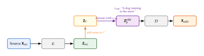
Proposition 43 (Edit Fidelity-Creativity Trade-off).
In Video SDEdit, the edit strength and source fidelity are controlled by the noise level :
Edit strength : as , the noisy latent approaches pure noise, and the denoising process generates content almost entirely from the edit prompt, giving maximum creative freedom.
Source fidelity : as , the noisy latent retains most of the source structure, and the edit is minimal.
Formally, if the source latent is Gaussian with covariance in dimensions, the mutual information between the source and the edited video is bounded by the capacity of the noising channel, (EDIT MI) which at reduces to . Since decreases monotonically with (from to ), the bound decreases with , confirming the trade-off. Only an inequality is available: denoising and decoding can destroy information but cannot create it, so the channel capacity is a ceiling on the retained information, not its value.
Proof.
Consider the noising process as a Gaussian channel. The source latent is observed through noise: . For Gaussian with covariance and independent Gaussian noise, the mutual information between and is This is monotonically decreasing in (since decreases), confirming that more noise reduces the information retained about the source. The data processing inequality then gives , since is obtained from by denoising and decoding, which establishes (EDIT MI). The step is one-directional: the chain gives no matching lower bound, so equality cannot be claimed.
Remark 84 (Practical guidelines for selection).
In practice, the optimal noise level depends on the type of edit:
Style transfer (e.g., “make it look like a watercolour painting”): . Low noise preserves the spatial structure while allowing texture changes.
Object modification (e.g., “change the red car to a blue car”): . Moderate noise allows colour and shape changes while preserving the overall scene layout.
Scene transformation (e.g., “change from day to night”): . Higher noise permits global illumination changes.
Major content change (e.g., “replace the city with a forest”): . Near-total noise is needed, but the camera motion from the source may still be loosely preserved.
Values below typically produce imperceptible edits, while values above are effectively unconditional generation with no memory of the source.
Caution.
Video SDEdit applies the same noise level to every frame simultaneously, which means every frame undergoes the same degree of modification. This makes spatially or temporally localised edits difficult. Changing only one object in the scene, or editing only a portion of the video's duration, requires additional mechanisms such as masking or attention manipulation.
The main limitation of Video SDEdit is that it processes the entire video uniformly: every frame receives the same noise level and the same editing prompt. This makes it difficult to perform localised edits (e.g., changing only one object) or edits that should affect different frames differently.
Attention injection for structure-preserving edits
A more sophisticated approach to video editing exploits the internal representations of the diffusion model, specifically the self-attention maps, to transfer structural information from the source video to the edited version. The key observation is that the self-attention keys and values in a diffusion U-Net or transformer encode the spatial layout and temporal structure of the content, while the queries drive the generation of new content.
Definition 78 (Attention Injection for Video Editing).
Let be a video diffusion model. Given source video and edit prompt , attention injection operates two parallel denoising branches:
Source branch: Perform DDIM inversion of to obtain noise maps . During reconstruction (denoising from ), record the self-attention keys and values at each layer and timestep.
Edit branch: Denoise from the same inverted noise , but conditioned on . At selected layers, replace the self-attention keys and values with those from the source branch: (Attention Injection)
The edit branch uses its own queries (driven by ) but the source branch's keys and values (encoding the source structure), resulting in edited content that follows the source layout.
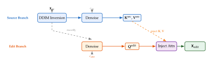
Advanced video editing methods
The basic SDEdit and attention injection techniques have been refined and extended in numerous ways. We highlight several influential approaches.
Example 54 (TokenFlow).
TokenFlow [46] addresses a fundamental limitation of per-frame editing approaches: even when each frame is edited consistently according to the prompt, the edits across frames may not be temporally coherent because the diffusion model processes each frame (or small batch of frames) independently. TokenFlow solves this by propagating the internal tokens (feature maps) of the diffusion model across frames according to the inter-frame correspondences established by the source video's optical flow.
Concretely, TokenFlow operates as follows. First, it performs DDIM inversion of the source video and records the intermediate features at each denoising step. Then, for each frame , it edits a sparse set of keyframes using any image editing method. Finally, it propagates the edited tokens to all other frames using the nearest-neighbour field computed from the source video's features. The propagation ensures that corresponding regions across frames receive consistent edits, even though the editing itself is performed independently per keyframe.
Example 55 (Pix2Video).
Pix2Video [47] takes an image editing approach and extends it to video through careful temporal propagation. The method first edits a single anchor frame using an image diffusion model (e.g., InstructPix2Pix). It then propagates the edit to neighbouring frames by injecting the self-attention features from the edited anchor into the denoising process of each subsequent frame. The propagation proceeds sequentially from the anchor frame outward, with each newly edited frame serving as the reference for the next.
Example 56 (FateZero).
FateZero [48] introduces the concept of “attention map blending” for zero-shot video editing. During DDIM inversion of the source video, FateZero stores not only the self-attention keys and values but also the cross-attention maps (the attention weights between spatial tokens and text tokens). During the editing pass, it blends the stored source attention maps with the new attention maps computed from the edit prompt, using a spatial mask to determine which regions should change and which should be preserved. The blending is expressed as (Fatezero Blend) where is a spatial mask derived from the cross-attention difference between source and edit prompts, is the all-ones matrix of the same shape, and denotes the attention maps.
Example 57 (Rerender-A-Video).
Rerender-A-Video [49] takes a hybrid approach that combines diffusion-based editing with optical-flow-based warping. It first edits a set of keyframes using an image diffusion model, then generates intermediate frames by (i) warping the nearest edited keyframe using optical flow from the source video, (ii) using the warped frame as the SDEdit initialisation for the diffusion model, and (iii) denoising with a small number of steps to clean up warping artifacts. The optical flow provides strong structural guidance, while the diffusion model handles disocclusions and artifacts that warping alone cannot resolve.
The method uses a cross-frame attention mechanism during the diffusion refinement step: each frame's self-attention keys and values are augmented with features from the nearest keyframe, encouraging consistency.
| Method | TF | Temporal | Local Edit | Quality |
| Video SDEdit | Yes | No | No | Medium |
| Attention Injection | Yes | Yes | No | High |
| TokenFlow | Yes | Yes | No | High |
| Pix2Video | Yes | Yes | No | Medium |
| FateZero | Yes | Yes | Yes | High |
| Rerender-A-Video | Yes | Yes | No | High |
Remark 85 (Comparing editing approaches).
Table 5 summarises the key trade-offs among the video editing methods discussed in this section. The choice of method depends on the type of edit, the available compute budget, and whether training-free operation is required.
Remark 86 (The inversion bottleneck).
Many video editing methods rely on DDIM inversion to obtain a noise-space representation of the source video. However, DDIM inversion is not exact: the deterministic inversion of DDIM is only approximately correct, and errors accumulate over the inversion steps. For images, these errors are small enough to be negligible, but for video, the accumulated error can cause noticeable artifacts, especially in fine details and at temporal boundaries. Several recent works address this through more accurate inversion schemes, such as null-text inversion or edit-friendly DDPM inversion, adapted to the video setting.
Exercise 46 (Designing a video editing pipeline).
You are tasked with building a system that takes a video of a person walking through a park and changes the season from summer to winter (adding snow, bare trees, overcast sky) while keeping the person's appearance and motion unchanged.
Would you use Video SDEdit or attention injection? Justify your choice.
What edit strength (as a fraction of ) would you recommend? What happens if is too low or too high?
How would you handle the person's appearance? They should remain unchanged, but SDEdit modifies the entire frame.
Propose a method that combines SDEdit with a segmentation mask to edit only the background.
Physics-Aware Video Generation and World Models
The videos we have discussed generating so far are evaluated primarily on visual quality and temporal consistency. A video of a ball bouncing might look beautiful, but does the ball actually follow a parabolic trajectory? Does it accelerate downward at ? Does it conserve momentum when it bounces? The frontier of video generation research asks a deeper question: can diffusion models learn not just the appearance of the physical world, but its dynamics?
This question connects video generation to the broader concept of world models: internal representations of how the world works that can be used for prediction, planning, and reasoning. If a video diffusion model can accurately predict what happens next in a physical scene, it is, in a meaningful sense, simulating physics. This section explores the theoretical foundations of this connection and surveys recent efforts to build physics-aware video generators.
World models: formalisation
The concept of a world model has a long history in cognitive science, control theory, and reinforcement learning. For our purposes, a world model is a conditional generative model that predicts future observations given past observations and (optionally) actions.
Definition 79 (World Model).
A world model is a function (World Model) where is the observed history (a sequence of video frames or state representations), is an optional action or intervention at time , is the prediction horizon, and is a distribution over future observations. When no action is provided (), the world model reduces to a pure prediction model.
The world model framework is general enough to encompass several important special cases.
Video prediction models (, ): predict the next frame given the past. These are the classical next-frame prediction models from the video prediction literature.
Interactive world models (): predict the visual consequence of taking action in the current state. These are directly relevant to robotics and game simulation.
Long-horizon world models (): predict extended future trajectories. These are the most ambitious and the most relevant to planning.
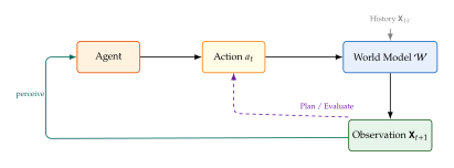
Physics-guided diffusion
One approach to incorporating physical knowledge into video generation is to use physics-guided diffusion: modifying the denoising process to steer generated videos toward physical plausibility. This is analogous to classifier guidance (Classifier-Free Guidance for Video), but instead of guiding with a classifier, we guide with a physics constraint.
Definition 80 (Physics-Guided Diffusion).
Let be the noise prediction of a video diffusion model, and let be a differentiable physics loss that measures how well a decoded video satisfies a given physical constraint (e.g., conservation of energy, Newtonian dynamics, fluid equations). Physics-guided diffusion modifies the noise prediction at each denoising step: (Physics Guided) where is the (frozen) decoder mapping latents to pixels, and controls the strength of the physics guidance.
Caution.
The physics loss must be evaluated on the Tweedie estimate of the clean video, never on directly. The decoder was trained on clean latents; feeding it a noisy latent produces an image outside its training distribution, so at moderate and high the resulting “physics residual” measures decoder failure rather than any physical property of the video, and its gradient points nowhere useful. Algorithm 8 implements the correct form.
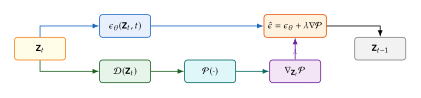
The physics loss can encode various physical constraints:
Conservation laws. Require that total energy, momentum, or mass is approximately conserved across frames: , where is an energy estimator applied to frame .
Trajectory constraints. Require that tracked object positions follow smooth, physically plausible trajectories: , where is the estimated acceleration and is gravitational acceleration.
Fluid dynamics. Require that observed flows satisfy the Navier-Stokes equations: , where is the estimated velocity field and are viscosity and pressure.
Rigid body constraints. Require that rigid objects maintain their shape: , where denotes pairwise distances between tracked points on the object.
Remark 87 (Computational cost of physics guidance).
Physics-guided diffusion requires backpropagating through the decoder - and, strictly, through as well, since depends on it - at every denoising step to compute . For large decoders and high resolutions, this gradient computation can be as expensive as the forward pass of the denoising model itself, roughly doubling the generation time. Implementations commonly place a stop-gradient on inside , which drops the second path at the cost of an approximate gradient. Gradient checkpointing, or applying guidance only at selected timesteps, further mitigates the cost.
Video diffusion as an implicit world model
A provocative hypothesis, articulated most prominently in the context of OpenAI's Sora [6], is that video diffusion models trained on sufficiently large and diverse video datasets may implicitly learn a world model. That is, without ever being explicitly trained on physics equations, they may learn to simulate the consequences of physical interactions from the statistical regularities present in the training data.
Theorem 10 (Video as Implicit World Model).
Let be the distribution of natural videos, and let be a generative model with sufficient capacity. If achieves for small , then for any physical constraint that is satisfied by natural videos with probability at least , (Implicit World Model) In words: a model that closely approximates the data distribution must also approximately satisfy any physical constraint that the data satisfies.
Proof.
By Pinsker's inequality, the total variation distance satisfies . Let . Then by assumption. By the definition of total variation distance, Therefore .
Key Idea.
Learning physics from pixels. Theorem 10 provides a theoretical basis for the empirical observation that large video models exhibit physical understanding. The argument is simple but powerful: if the real world obeys physics, and the model faithfully captures the distribution of real-world videos, then the model's outputs will also (approximately) obey physics. No explicit physics knowledge is required; it emerges as a consequence of distributional matching.
However, several important caveats temper this optimistic view.
Remark 88 (Limitations of Implicit World Models).
While Theorem 10 is mathematically correct, it relies on strong assumptions that are not satisfied in practice:
Conservation laws. Physical conservation laws (energy, momentum, charge) are exact in the real world but only approximately represented in the training data (due to camera angles, occlusions, and limited video duration). A model matching the data distribution inherits these approximate representations, not the exact laws, and may violate conservation in scenarios that are physically possible but rare in the training set.
Counting and combinatorics. Current video models notoriously struggle with counting: a video of five balls bouncing may show four or six balls in some frames. This is because counting is a discrete, global constraint that is poorly captured by the local pattern-matching that diffusion models excel at.
Novel scenarios. The guarantee in Theorem 10 holds only for scenarios represented in the training distribution. For out-of-distribution scenarios (e.g., zero-gravity environments, novel materials), the model has no basis for correct physical reasoning and will default to the most similar training examples, which may exhibit entirely wrong physics.
Long-horizon accuracy. Even if the model accurately predicts one or two frames ahead, errors compound over longer horizons (recall Proposition 39). Physical simulations require exponentially growing precision over time to maintain accuracy; neural models cannot provide this.
Frontier systems: Sora and beyond
The connection between video generation and world modelling was thrust into the spotlight by OpenAI's Sora [6], which was described as a “world simulator.” Let us examine what this claim means and what evidence supports or qualifies it.
Example 58 (Sora as a World Simulator).
Sora generates videos by operating on sequences of spacetime patches processed by a Diffusion Transformer (DiT). Its training on a massive corpus of internet video, combined with the DiT architecture's ability to model long-range dependencies, enables several behaviours suggestive of world understanding:
3D consistency: camera movements produce parallax effects consistent with a 3D scene, suggesting that the model has learned implicit 3D representations.
Object permanence: objects that leave the frame return with consistent appearance, and objects partially occluded by other objects are completed plausibly when revealed.
Approximate dynamics: balls roll, water flows, and cloth drapes in approximately correct ways, suggesting learned physical priors.
Interaction effects: actions like stepping in sand leave footprints, and interactions between objects produce plausible consequences.
However, Sora also exhibits clear failures of physical reasoning: objects sometimes pass through each other, liquids defy gravity, and complex multi-body dynamics are often incorrect, confirming the limitations outlined in Remark 88.
Example 59 (UniSim).
UniSim [50] explicitly trains a video diffusion model as an interactive world model. Given a current observation and an action (specified as text, e.g., “turn left” or “pick up the red block”), UniSim predicts the next observation. The model is trained on a combination of real-world video with action labels (from robotics datasets) and synthetic data from game engines. UniSim demonstrates that video diffusion models can serve as effective visual simulators for training robotic policies, achieving comparable performance to policies trained in ground-truth simulators on several manipulation tasks.
Example 60 (GameGen-X and Genie).
GameGen-X [51] and Genie [52] represent the frontier of interactive world models for game environments. GameGen-X is specifically designed for open-world game video generation, producing interactive gameplay videos conditioned on user inputs (keyboard and mouse actions). Genie, developed by Google DeepMind, learns a “world model from internet videos” by jointly learning a video tokeniser, a dynamics model, and an action model. Genie's key insight is that actions need not be provided during training; they can be inferred as the latent variables that explain transitions between frames. This makes it possible to train interactive world models from unlabelled video, a significant step toward scalable world model learning.
The connection between world models and agentic AI is deep and actively explored. We refer the reader to 27 for a thorough treatment of how world models can be used for planning and decision-making in agentic systems, and to 23 for the relationship between world modelling and recursive reasoning.
Algorithm 8 (Physics-Guided Video Generation).
Given a text prompt , a physics constraint , and guidance strength :
Sample initial noise .
For : enumerate
Compute model prediction: .
Estimate clean video: .
Compute physics gradient: .
Apply guidance: , where is a timestep-dependent weight (typically larger at intermediate timesteps).
Update: . enumerate
Return .
Remark 89 (Choosing the guidance schedule ).
The guidance strength should vary across timesteps. At early steps (large ), the clean-video estimate is noisy and unreliable, so physics gradients computed from it are inaccurate; guidance should be weak. At late steps (small ), the estimate is much cleaner and gradients are meaningful; guidance should be stronger. A common choice is the “warm-up” schedule , which ramps the guidance from zero at to full strength after steps.
The gap between simulation and understanding
There is an important philosophical and practical distinction between a model that simulates physics and one that understands physics. A video diffusion model that produces realistic-looking bouncing balls is performing high-fidelity pattern matching against its training distribution. Whether this constitutes “understanding” of Newtonian mechanics is a matter of definition and debate.
We can formalise this distinction using the concept of generalisation depth: how far beyond the training distribution a model's physical predictions remain accurate.
Definition 81 (Generalisation Depth).
The generalisation depth of a world model with respect to a physical law is the maximum perturbation magnitude such that (Generalisation Depth) where is the data distribution perturbed by in some relevant parameter (e.g., gravity, friction, initial conditions), is the ground-truth physical prediction, and is the acceptable error threshold.
A model with high generalisation depth has learned something closer to the underlying physical law rather than merely memorising surface statistics. Current video diffusion models have low generalisation depth: they produce plausible-looking physics for scenarios similar to their training data, but fail rapidly when physical parameters are perturbed beyond the training range.
Insight.
The question “does a video diffusion model understand physics?” is ill-posed without defining “understand.” If understanding means “can generate outputs consistent with physical laws in scenarios seen during training,” then yes, large video models understand physics. If understanding means “can reason about novel physical scenarios, derive consequences of perturbed initial conditions, or discover new physical laws,” then no, current video models do not understand physics. The truth lies in the gap between interpolation (recombining patterns from training data) and extrapolation (generalising to genuinely novel situations). Video models are spectacular interpolators but limited extrapolators.
| Category | Example | Current | Difficulty |
| Accuracy | |||
| Gravity | Ball falling | High | Easy |
| Inertia | Sliding object | High | Easy |
| Collision | Billiard balls | Medium | Medium |
| Fluid dynamics | Water pouring | Medium | Medium |
| Deformation | Cloth folding | Medium | Medium |
| Multi-body | Newton's cradle | Low | Hard |
| Conservation | Energy in bounce | Low | Hard |
| Counting | Fixed # of objects | Low | Hard |
| Novel physics | Zero gravity | Very low | Very hard |
Exercise 47 (Evaluating physical understanding).
Design an evaluation benchmark for testing whether a video generation model understands basic physics. Your benchmark should include:
Five test scenarios spanning different physical phenomena (e.g., projectile motion, fluid dynamics, rigid body collisions, elastic deformation, buoyancy).
For each scenario, a quantitative metric comparing the generated trajectory to the ground-truth physics simulation.
A distinction between “interpolation” tests (scenarios similar to training data) and “extrapolation” tests (scenarios requiring generalisation, e.g., unusual gravity or novel materials).
A discussion of how your benchmark handles the stochasticity inherent in diffusion models (different random seeds produce different videos).
Exercise 48 (Physics-guided diffusion implementation).
Consider a video generation task where a ball is thrown upward and must follow a parabolic trajectory.
Write the physics loss for this scenario, assuming you have a differentiable ball detector that returns the position of the ball in each frame.
The ball detector outputs a soft heatmap. How does this affect the gradient ?
Estimate the computational overhead of physics guidance relative to standard generation, assuming the ball detector is a small network ( of the diffusion model's parameters).
What happens if the physics loss conflicts with the text prompt (e.g., prompt says “floating ball” but physics loss enforces gravity)? How would you handle this?
Autoregressive-Diffusion Hybrids
Throughout this chapter, we have treated diffusion as the primary generative mechanism for video. But diffusion is not the only game in town. Autoregressive models, which generate data one token at a time conditioned on all previous tokens, have been spectacularly successful in language modelling and have shown promise for visual generation through vector-quantised tokenisation. A natural question arises: can we combine the strengths of both paradigms?
The basic intuition behind autoregressive-diffusion hybrids is straightforward: autoregressive models excel at capturing long-range dependencies and sequential structure (they “know what to generate”), while diffusion models excel at producing high-quality continuous outputs (they “know how to generate it”). Combining them should yield models that can plan over long temporal horizons while producing visually strong results.
A caution before we proceed. This is a design space, not yet a settled family of systems, and the literature is looser with the word “hybrid” than it should be. Several of the systems routinely cited under this heading are not hybrids at all: they are pure autoregressive token models whose detokeniser happens to be a strong learned decoder. We will therefore describe the two architectural patterns first, and then place named systems on the resulting spectrum honestly - including those that turn out to sit at its endpoints rather than in the middle.
Frame-level AR with per-frame diffusion
The simplest hybrid architecture generates the video one frame at a time, using an autoregressive backbone to model the temporal sequence and a diffusion model to generate each frame's content.
Definition 82 (AR-Diffusion Hybrid (Frame-Level)).
An autoregressive-diffusion hybrid at the frame level factorises the video distribution as (AR Diffusion Frame) where is the distribution of the first frame (itself potentially generated by a diffusion model) and is a conditional diffusion model that generates frame given all previous frames .
The conditioning on can be implemented in several ways:
Direct concatenation. Concatenate the previous frames (or their latent encodings) to the noisy input of the diffusion model along the channel or temporal dimension. This is simple but scales poorly with context length.
Cross-attention conditioning. Encode the previous frames into a sequence of feature vectors and inject them via cross-attention in the denoising network. This scales better but requires careful attention to the memory cost.
Recurrent state conditioning. Process the previous frames through a recurrent network (LSTM, GRU, or state-space model) to produce a fixed-size hidden state, and condition the diffusion model on this state. This has constant memory cost regardless of context length but compresses the history lossy.
The frame-level hybrid inherits both the strengths and weaknesses of autoregressive generation. On the positive side, it can generate videos of arbitrary length (each frame is generated independently conditioned on the past), and the diffusion model ensures high per-frame quality. On the negative side, it suffers from the same error accumulation as autoregressive chunk generation (Proposition 39), and generation is inherently sequential (each frame must wait for all previous frames), eliminating the parallel sampling advantage of full-video diffusion.
Remark 90 (Latency analysis).
The latency of a frame-level AR-diffusion hybrid is dominated by the sequential nature of the autoregressive loop. For a video of frames where each diffusion generation requires denoising steps, the total latency is model evaluations. Compare this to pure diffusion over the full video, which requires only evaluations (though each evaluation processes the full -frame tensor). The frame-level hybrid is therefore slower by a factor of in latency, but each evaluation is cheaper by a factor related to (processing one frame versus frames). The total compute is roughly comparable, but the wall-clock time is worse for the hybrid when parallelism across frames is available.
Temporal AR, spatial diffusion
A more sophisticated hybrid decouples the temporal and spatial aspects of generation: an autoregressive model handles the temporal sequence of compact representations, and a diffusion model handles the spatial rendering of each representation into a full frame.
Definition 83 (Temporal AR, Spatial Diffusion).
The temporal AR, spatial diffusion hybrid introduces a sequence of compact latent codes , one per frame (e.g. a quantised token or a low-dimensional embedding), and models the joint distribution of codes and video as (Temporal AR Spatial DIFF Joint) The video distribution is the marginal of this joint, which requires summing (or integrating) over the codes: (Temporal AR Spatial DIFF) with the sum replaced by an integral when the codes are continuous. Sampling never performs this marginalisation explicitly: one draws and then , which is an exact draw from the joint and hence from the marginal. Likelihood evaluation, by contrast, is intractable for exactly this reason, and the codes act as latent variables rather than as observed conditioning.
This factorisation has a clean interpretation: the autoregressive model serves as a “director,” planning what happens at each point in the video, while the diffusion model serves as a “renderer,” producing the high-quality visual output. The codes capture semantic content (object positions, actions, scene changes) while abstracting away pixel-level details (textures, lighting, exact colours) that the diffusion model handles.
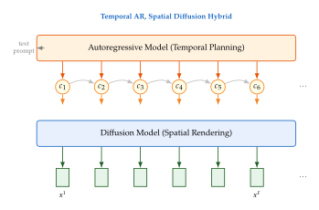
Named systems on the AR–diffusion spectrum
The systems usually gathered under the “hybrid” heading do not all contain both mechanisms. It is worth being precise about which do, because the distinction is exactly the one this section is about.
Example 61 (Emu Video: a two-stage cascade).
Emu Video [53] is the cleanest illustration of the plan-then-render idea. It factorises text-to-video generation into two explicit stages: (1) text-to-image generation using a high-quality image diffusion model, producing a single keyframe; and (2) image-to-video generation using a video diffusion model conditioned on both the text prompt and the generated keyframe.
The advantage is simplicity: each stage can be trained independently, the image stage benefits from the much larger corpus of image-text pairs, and the video stage has a strong visual anchor that promotes temporal consistency. It should be labelled accurately, though: both stages are diffusion models. Emu Video separates planning from rendering, which is the structural idea of Temporal AR, spatial diffusion, but the “plan” is a single image and there is no autoregressive component at all. It is a cascade, not an AR-diffusion hybrid.
Example 62 (VideoPoet: the pure autoregressive endpoint).
VideoPoet [54], developed by Google Research, is a decoder-only language model that generates video through a two-stage process. First, video is tokenised into discrete codes by a MAGVIT-v2 tokeniser (17-frame clips become 1,280 tokens; single images become 256 tokens). Then an autoregressive transformer generates sequences of video tokens conditioned on text tokens, image tokens, audio tokens, or any combination thereof. Audio is tokenised separately with SoundStream, and a low-resolution generation is upsampled by a super-resolution stage.
VideoPoet contains no diffusion model anywhere. The tokeniser is a vector-quantised autoencoder, not a diffusion autoencoder; its decoder is a feed-forward reconstruction network. The super-resolution stage is a non-autoregressive, bidirectional transformer over tokens; it borrows classifier-free guidance from the diffusion literature, but guidance is a sampling technique, not a diffusion process. VideoPoet therefore belongs in this section as the pure autoregressive endpoint of the spectrum - the system a genuine hybrid has to beat - and not as an example of the hybrid thesis.
What VideoPoet does demonstrate is task unification: a single model handles text-to-video, image-to-video, video-to-video, video editing and video-to-audio by formatting each as a sequence-to-sequence problem with appropriate token types. That is the video analogue of the foundation-model paradigm in NLP, and it is a property of the token interface rather than of any particular generative mechanism.
Example 63 (MAGVIT-v2 + Language Model).
MAGVIT-v2 [55] introduces a “lookup-free quantisation” scheme that enables video tokenisation with a vocabulary of exactly codes without the codebook collapse problems that plague standard vector quantisation. Its core innovation is in the tokeniser: standard VQ-VAE approaches struggle with video because most codebook entries go unused, and lookup-free quantisation removes the codebook entirely by quantising each latent vector with the sign of each of its dimensions, producing a binary code read off as a token index. This guarantees full utilisation of the implicit vocabulary and makes the large sizes needed for high-fidelity video representation practical.
Paired with a language model as the autoregressive backbone, this gives a system whose sample quality is competitive with continuous diffusion models on standard benchmarks - the point of the paper's title, “Language Model Beats Diffusion” - while retaining the scalability and versatility of language model architectures. Like VideoPoet, and for the same reason, this is an autoregressive system rather than a hybrid: the argument it makes is that a good enough tokeniser removes the need for diffusion, not that the two should be combined.
Remark 91 (Where the genuine hybrids are).
The three systems above bracket the design space without occupying its middle. Genuine AR-diffusion hybrids - models in which an autoregressive backbone emits continuous states and a diffusion head renders or refines them, so that both mechanisms are present in a single generative pass - are a more recent and still less settled development; the continuous-token direction sketched in Remark 93 is where they live. The patterns in Architectural patterns for hybrids are therefore best read as a map of what is possible, with the warning that the best-known named systems currently sit at the edges of that map rather than at its centre.
Theoretical comparison of paradigms
To understand why hybrids are attractive, consider the complementary strengths and weaknesses of the pure paradigms.
| Property | Pure AR | Pure Diffusion | Hybrid |
| Long-range planning | Strong | Weak | Strong |
| Per-frame quality | Medium | Strong | Strong |
| Generation speed | Slow | Medium | Medium |
| Variable length | Native | Requires tricks | Native |
| Multi-modal integration | Native | Requires adapters | Native |
| Training data needs | Tokenised video | Continuous video | Both |
| Drift over a rollout | Linear in steps | None within window | Intermediate |
Remark 92 (The convergence of paradigms).
An interesting trend in the field is the gradual convergence of autoregressive and diffusion approaches. Masked diffusion models can be viewed as non-autoregressive versions of masked language models. Autoregressive models with continuous outputs (like those using diffusion loss instead of cross-entropy) are essentially diffusion models with autoregressive structure. Flow matching can be applied both to continuous data (as in standard diffusion) and to discrete tokens (as in discrete flow matching). This convergence suggests that the “AR versus diffusion” distinction may be less fundamental than it appears, and that the most effective future systems will seamlessly blend both paradigms.
Architectural patterns for hybrids
Several architectural patterns have emerged for building hybrid systems.
Pattern 1: Token-then-render. Generate discrete tokens autoregressively, then render continuous outputs from those tokens. VideoPoet and MAGVIT-v2 + LM take this route with a feed-forward VQ decoder as the renderer, which is what makes them autoregressive rather than hybrid; the pattern becomes a hybrid only when the renderer is itself a conditional diffusion model. The advantage either way is a clean separation of concerns; the disadvantage is that quantisation introduces an information bottleneck (Proposition 44).
Pattern 2: Plan-then-diffuse. Generate a coarse plan (keyframes, layout, motion trajectory) autoregressively, then generate the full video conditioned on the plan using diffusion. This is related to the hierarchical keyframe generation of Hierarchical keyframe generation and to Emu Video's two-stage approach. The advantage is that the AR component operates in a much lower-dimensional space; the disadvantage is that the plan must capture enough information to guide the diffusion model.
Pattern 3: Interleaved AR-diffusion. Alternate between autoregressive steps (generating a new token or code) and diffusion steps (refining the current output). This is the most tightly coupled pattern and the hardest to train, but it allows the AR and diffusion components to inform each other throughout the generation process.
Exercise 49 (Designing a hybrid architecture).
You are designing a text-to-video model for generating 30-second clips at 720p resolution.
Compare the three architectural patterns (token-then-render, plan-then-diffuse, interleaved) in terms of training complexity, generation speed, and expected quality.
For the plan-then-diffuse pattern, what should the “plan” consist of? Consider at least three options (e.g., keyframes, text descriptions, layout maps) and discuss their trade-offs.
How would you handle the text prompt in each pattern? In some patterns, the text directly conditions the AR model; in others, it conditions the diffusion model; in some, both.
Estimate the generation time for a 30-second, 720p video using each pattern, assuming a single A100 GPU. State your assumptions about model size, token count, and diffusion steps.
Proposition 44 (Information Bottleneck in Token-Based Hybrids).
In a token-then-render hybrid, the video tokeniser maps each frame to discrete tokens from a codebook of size . The maximum information per frame is bits. For a codebook of size and tokens per frame, this gives bits per frame. A raw 720p RGB frame contains approximately bits. The compression ratio is therefore approximately .
The quality of the hybrid system is fundamentally limited by how much perceptually relevant information is preserved through this bottleneck. If the tokeniser discards information that the diffusion renderer cannot reconstruct, no amount of training will recover it.
Proof.
The information bound follows directly from the capacity of the discrete channel. Each of tokens can take one of values, giving possible configurations. The information content is bits. The compression ratio is the ratio of raw bits to token bits: . Substituting the given values yields .
Remark 93 (Beyond discrete tokenisation).
The information bottleneck of discrete tokenisation has motivated research into continuous token hybrids, where the AR model generates continuous-valued representations rather than discrete indices. In this setting, the AR model predicts each “token” as a continuous vector, potentially using a diffusion loss (rather than cross-entropy) for the per-token prediction. This eliminates the quantisation bottleneck at the cost of requiring different training objectives and sampling procedures. Models such as MAR (Masked Autoregressive generation) explore this direction, blurring the line between AR and diffusion even further.
Key Idea.
Separate the planning from the rendering. The durable idea in this section is not that every system should contain both an autoregressive and a diffusion component, but that what happens and how it looks are separable concerns, and that each can be assigned to whichever mechanism suits it. Delegating temporal planning to an autoregressive backbone and spatial rendering to a diffusion model is the most ambitious version of that split; assigning both roles to diffusion (Emu Video) or both to autoregression (VideoPoet) are the currently better-demonstrated ones. What is genuinely converging is the machinery - masked diffusion resembles masked language modelling, autoregressive models with a diffusion loss resemble diffusion models with sequential structure - so the label attached to a system is becoming a weaker guide to what is inside it than the question of which component does the planning.
Exercise 50 (Tokenisation quality analysis).
Consider a video tokeniser that maps each spatial patch of a video frame to a single discrete token from a codebook of size .
How many tokens represent one frame? What is the information content per frame as a function of ?
Good-quality H.264/H.265 encodings of natural video run at roughly to bits per pixel. For what range of does the token budget match that rate? (Express your answer as a range for .)
MAGVIT-v2 uses . What bit rate per pixel does that correspond to under this tokenisation? Is it above or below the codec range from part (b)? Given that the answer is “below,” name two reasons a learned tokeniser can nevertheless produce acceptable video at that rate - and one reason the comparison is not entirely fair to either side.
Propose a metric for evaluating tokenisation quality that goes beyond reconstruction PSNR. Consider temporal aspects specific to video.
Historical Note.
From rivalry to synthesis. The autoregressive and diffusion paradigms developed largely in parallel. Autoregressive visual generation emerged from the VQ-VAE line of work (van den Oord et al., 2017), which demonstrated that images could be represented as sequences of discrete tokens and generated by powerful sequence models. VideoGPT [2] extended this to video, using VQ-VAE tokenisation followed by GPT-style generation. Meanwhile, diffusion models for video emerged from the image diffusion revolution (Ho et al., 2020), with Video Diffusion Models [3] demonstrating the viability of joint space-time denoising.
By 2023–2024 the two lines had converged in capability rather than in architecture. MAGVIT-v2 and VideoPoet showed that a sufficiently good tokeniser lets a pure autoregressive model match diffusion quality, while Emu Video showed that decomposing generation into a planning stage and a rendering stage pays off even when both stages are diffusion models. The synthesis suggested by these results is not that every system should contain both mechanisms, but that the separation of planning from rendering is the durable idea, and that either mechanism can be dropped into either role. Architectures that place a diffusion head on an autoregressive backbone, so that both are present in a single generative pass, are the current frontier of that idea rather than its established form.
Everything so far has been about building video generators. The remainder of the chapter asks how we know whether any of it worked. We turn next to evaluation - the Fréchet Video Distance and its reading as a Wasserstein distance, the decomposed sixteen-dimensional VBench protocol, the temporal-consistency metrics of Temporal Consistency Metrics, and human evaluation protocols - and then to specialised applications that reuse the same backbone with different conditioning: human motion generation, audio-visual generation, talking-head synthesis and virtual try-on. We close by wiring the chapter into the rest of the book, from variational inference and optimal transport to memory architectures and agentic world models, and by stating five open problems that define the current frontier: real-time generation, minute-scale consistency, physical grounding, compositional generation, and unified multimodal generation.
Evaluation Metrics for Video Generation
Generating videos is only half the challenge; the other half is measuring whether the generated videos are any good. Unlike image generation, where the Fréchet Inception Distance (FID) [73] has become a near-universal yardstick, the evaluation of video generation models must contend with an additional temporal dimension that fundamentally complicates quality assessment. A video can have excellent per-frame quality yet exhibit temporal flickering; it can be temporally smooth yet lack diversity; it can match the data distribution in aggregate statistics yet fail to produce physically plausible motion.
In this section, we formalise the principal evaluation metrics used in the field, analyse their mathematical properties, and discuss their strengths and limitations. We begin with the Fréchet Video Distance (FVD), the most widely used automatic metric for video generation, and then turn to the more recent decomposed evaluation frameworks that aim to capture the multifaceted nature of video quality.
Fréchet Video Distance
The Fréchet Video Distance extends the FID from images to video by replacing the Inception-v3 feature extractor with a video-aware network, typically an Inflated 3D ConvNet (I3D) [74]. The I3D network processes short video clips and produces a feature vector that captures both spatial appearance and temporal dynamics.
Definition 84 (Fréchet Video Distance).
Let be a set of real video clips and a set of generated video clips. Let be a feature extractor (typically I3D with ). Define the empirical mean and covariance of the real and generated feature sets: (FVD Stats REAL) The Fréchet Video Distance is (FVD)
The FVD inherits the mathematical structure of the FID and admits a clean interpretation in terms of optimal transport.
Theorem 11 (FVD as Wasserstein Distance).
Let and be the Gaussian distributions fitted to the real and generated feature sets, respectively. Then (FVD W2) where denotes the -Wasserstein distance (see 14 for a comprehensive treatment of optimal transport distances).
Proof.
The squared -Wasserstein distance between two Gaussians and on is given by the Dowson–Landau–Olkin–Pukelsheim formula: (W2 Gaussian) To see this, recall from 14 that the optimal transport map between two Gaussians is affine. Specifically, the optimal coupling between and is itself Gaussian with marginals and , and the transport cost under the squared Euclidean distance is (W2 Expansion) Using the identity for positive semi-definite and (with ), we simplify the last term to , yielding exactly the FVD formula (FVD).
Remark 94 (Connection to FID).
The FVD is structurally identical to the FID introduced in 4; the only difference is the choice of feature extractor. FID uses Inception-v3 features computed from individual images, while FVD uses I3D features computed from video clips. Because I3D processes multiple frames jointly, its features encode temporal patterns (motion direction, speed, periodicity) that are invisible to a per-frame image feature extractor.
FVD Computation Pipeline
Figure 38 illustrates the end-to-end computation of FVD. The pipeline has four stages: (i) sample real and generated clips, (ii) extract I3D features from each clip, (iii) compute the sample mean and covariance of each feature set, and (iv) evaluate the closed-form FVD expression.
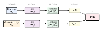
Example 64 (FVD in practice).
When computing FVD, several practical details matter:
Sample size. FVD is a biased estimator: with too few samples, the covariance matrices are poorly estimated, leading to unreliable scores. The community convention is to use at least clips, following the recommendation of Unterthiner et al. [56].
Clip length. The I3D network expects clips of a fixed length (typically 16 frames at 224224 resolution). Longer generated videos must be split into non-overlapping 16-frame segments, and FVD is computed over the pooled set of segments.
Resolution alignment. Both real and generated clips must be resized to the same resolution before feature extraction. Resolution mismatches introduce systematic biases in the feature statistics.
Random seed sensitivity. FVD can vary significantly across different random samples from the generation model. Reporting the mean and standard deviation over multiple evaluation runs is essential for reliable comparison.
Limitations of FVD
Despite its widespread use, FVD has several well-known limitations.
Caution.
FVD is a single number for a multidimensional problem. The FVD collapses the entire distribution of video quality into a scalar. Two models with the same FVD can differ dramatically in their failure modes: one might produce temporally smooth but visually bland videos, while the other produces high-fidelity frames with occasional temporal glitches. FVD cannot distinguish between these failure modes because it aggregates over all aspects of quality simultaneously. Furthermore, the I3D features were trained for action recognition, not video quality assessment, so FVD may be insensitive to artifacts that are perceptually important but irrelevant to action classification.
Additional limitations include the following:
Gaussian assumption. FVD assumes that the feature distributions are well-approximated by Gaussians. If the true feature distribution is multimodal (as it typically is for diverse video datasets), the Gaussian fit discards important structural information.
Feature extractor bias. The I3D network was trained on the Kinetics dataset, which is dominated by human actions. FVD may therefore be more sensitive to motion quality in human-centric videos than in scenes involving natural phenomena, animals, or abstract content.
No per-sample quality. FVD is a distributional metric: it compares two sets of videos, not individual samples. It cannot tell you whether a specific generated video is good or bad.
Temporal resolution. The 16-frame input window of I3D limits FVD's ability to detect long-range temporal inconsistencies that manifest over seconds rather than fractions of a second.
Decomposed Evaluation: VBench
Recognising the limitations of single-number metrics, Huang et al. [57] introduced VBench, a comprehensive evaluation framework that decomposes video quality into 16 interpretable dimensions. The key insight is that “video quality” is not a monolithic concept but a composite of many independent axes, each of which can be measured separately and improved independently.
Definition 85 (VBench Decomposition).
The VBench framework evaluates a video generation model along 16 dimensions, grouped into two categories: seven that measure the intrinsic quality of the generated video irrespective of the prompt, and nine that measure whether the video actually depicts what the prompt asked for.
Video quality dimensions (seven; measuring the intrinsic quality of generated videos, computable without reference to the prompt): enumerate[label=()]
Subject consistency
Background consistency
Temporal flickering
Motion smoothness
Dynamic degree
Aesthetic quality
Imaging quality enumerate
Video–condition consistency dimensions (nine; measuring semantic faithfulness to the text prompt): enumerate[label=(), resume]
Object class
Multiple objects
Colour
Spatial relationship
Scene
Overall consistency
Human action
Temporal style
Appearance style enumerate
Note that “object class”, “multiple objects”, “colour”, “spatial relationship” and “scene” are semantic axes: they ask whether the prompted content is present, not whether the pixels look good. They therefore belong to category B, not to the quality group. Each dimension for is measured by a specialised evaluator that returns a scalar score .
The decomposed nature of VBench allows researchers to diagnose specific weaknesses in their models. A model that scores poorly on “temporal flickering” but well on “imaging quality” clearly has a temporal consistency problem, not a per-frame quality problem. This diagnostic power is impossible with FVD alone.
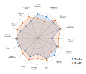
Temporal Consistency Metrics
Beyond FVD and VBench, a family of lightweight metrics specifically targets temporal consistency, the quality that distinguishes a coherent video from a slideshow of pretty pictures.
Definition 86 (CLIP-Based Temporal Consistency).
Given a generated video and a CLIP image encoder , the CLIP temporal consistency score is (TC CLIP) The score is bounded above by , attained exactly when all frames map to identical CLIP embeddings, and decreases as inter-frame variation grows. It is not bounded below by : for approximately unit-norm CLIP embeddings each summand is , reaching for orthogonal embeddings and for antipodal ones, so . A negative score therefore indicates that consecutive frames are, on average, semantically unrelated - a hard cut, or a catastrophic generation failure.
Caution.
Two different metrics are called “temporal consistency”. (TC CLIP) is a semantic score built from consecutive CLIP embeddings. It is a different quantity from the flow-warped perceptual similarity of Definition 74, which warps frame back onto frame using optical flow and compares them in a perceptual feature space. The two answer different questions - “does the video keep depicting the same thing?” versus “is the pixel motion physically consistent?” - and a video can score well on one and badly on the other. We write throughout this section to keep them apart.
Remark 95 (Interpreting temporal consistency).
The score measures semantic consistency rather than pixel-level consistency. Two frames that depict the same scene from slightly different viewpoints will have similar CLIP embeddings and thus a high score, even though their pixel values differ substantially. This is a feature rather than a bug: the metric captures the perceptually relevant notion that the video depicts a coherent scene, without penalising natural motion.
Proposition 45 (Bounds on CLIP Temporal Consistency).
If the CLIP encoder maps all natural images to vectors of approximately unit norm (i.e., for all ), then the temporal consistency score simplifies to (TC Simplified) where is the average consecutive-frame distance in CLIP space. Furthermore, by the triangle inequality applied along the chain , (TC Triangle) and hence (TC Upper)
Caution.
This bound is weak, and weakens as grows. It is tempting to read (TC Upper) as saying that a video whose first and last frames are semantically distant must score badly. It says no such thing. The right-hand side of (TC Triangle) is : with unit-norm embeddings the numerator is at most , so for a -frame clip the bound only forces even in the worst case. Total semantic drift can be spread arbitrarily thinly over many frames without ever registering. This is a structural weakness of any mean-of-consecutive-differences score: it measures local smoothness and is nearly blind to global drift. That is precisely why identity- and background-preservation metrics that compare distant frame pairs directly - such as the minimum-over-pairs identity score of Definition 75 - must be reported alongside it, and why VBench keeps “subject consistency” as a separate dimension from “temporal flickering”.
In addition to CLIP-based metrics, several other temporal quality measures are commonly used:
Warping error: Given optical flow between frames and , the warping error measures how well frame can be reconstructed by warping frame : (WARP Error) where warps frame using flow via bilinear interpolation (the same warping operator used in Definition 74; we avoid the symbol , which Definition 79 reserves for the world model).
Subject identity preservation : A face recognition model (e.g., ArcFace) extracts embeddings from detected faces across frames, and the cosine similarity between consecutive embeddings is averaged. This is particularly relevant for talking-head and character animation applications.
Motion magnitude score : The average optical flow magnitude measures the overall dynamic degree of the video. A video with is essentially a static image, which may indicate a degenerate generation mode even if FVD is low.
Human Evaluation Protocols
Automatic metrics, no matter how sophisticated, remain imperfect proxies for human perception. For this reason, human evaluation remains the gold standard for assessing video generation quality.
The most common protocol is the two-alternative forced choice (2AFC): evaluators are shown pairs of videos (one real, one generated, or two generated by different models) and asked to choose which is more realistic or better matches a text prompt. The fraction of times a model's output is preferred yields a win rate that is directly interpretable.
A more nuanced protocol decomposes the evaluation into separate dimensions, mirroring the VBench structure. Evaluators are asked to rate each video on temporal consistency, visual quality, motion naturalness, and text alignment on a Likert scale (e.g., 1 to 5). This decomposed human evaluation is expensive (typically requiring hundreds of evaluators and thousands of judgements) but provides the most reliable signal for model comparison.
Insight.
Automatic metrics correlate imperfectly with human judgement. The human studies reported alongside both the FVD [56] and VBench [57] proposals find only moderate agreement between automatic rankings and human preference rankings. How moderate depends on the dataset, the pool of models being ranked, and the evaluation protocol, so no single correlation coefficient is worth quoting as a property of the metric. VBench dimensions tend to correlate better individually with their corresponding human judgement axes, because each is validated against annotations for that axis alone; but no automatic metric fully captures the holistic “does this look like a real video?” assessment that humans perform effortlessly. For this reason, papers that claim state-of-the-art video generation quality should always include human evaluation alongside automatic metrics.
Evaluation Summary
Table 8 compares the key evaluation approaches discussed in this section.
| Metric | Type | Strengths | Weaknesses | Best for |
| FVD | Distributional | Single number; widely used; cheap to compute; I3D features do see motion | 16-frame window hides long-range drift; Gaussian fit; no per-sample score | Quick comparisons across models |
| VBench | Decomposed | Diagnostic; 16 dimensions; interpretable | Complex to set up; evaluator-dependent | Identifying specific failure modes |
| Per-video | Lightweight; semantic level | Local only: nearly blind to slow global drift | Temporal consistency screening | |
| Warping error | Per-video | Pixel-level; motion-aware | Requires flow estimation; sensitive to occlusion | Motion quality assessment |
| Human eval | Perceptual | Gold standard; holistic | Expensive; slow; subjective | Final model comparison |
Specialised Applications
The general-purpose text-to-video pipeline developed in the preceding sections can be specialised to a remarkable variety of application domains. In each case, the core diffusion backbone remains largely unchanged; what differs is the conditioning signal, the data domain, and the task-specific loss functions or architectural adaptations. In this section, we survey four particularly active application areas: human motion generation, audio-visual synthesis, talking head generation, and virtual try-on.
Human Motion Generation
Human motion generation aims to synthesise realistic sequences of body poses, typically represented as trajectories of joint positions or rotations over time. Unlike pixel-space video generation, the output is a structured skeletal sequence, making the problem both lower-dimensional and more constrained.
Definition 87 (Skeletal Motion Sequence).
A skeletal motion sequence of frames with joints is a tensor , where the -th frame specifies the position (or rotation) of each joint. Common choices are:
Joint positions: is the 3D world coordinate of joint in frame , giving .
Joint rotations: encodes the 6D continuous rotation representation of joint relative to its parent in the kinematic chain, giving .
Joint velocities: captures the per-frame displacement, useful for motion that must begin and end at specified poses.
For a standard 22-joint human skeleton with and (corresponding to 4 seconds at 30 fps), the total dimensionality is , many orders of magnitude smaller than the pixel-space representation of the corresponding video.
Insight.
Motion generation is diffusion in a structured, low-dimensional space. Because skeletal representations are compact and obey kinematic constraints (fixed bone lengths, joint angle limits), the diffusion process operates in a space where the manifold of valid motions is much better behaved than the manifold of natural images. This makes the denoising task easier: the model need not learn to synthesise textures, lighting, or backgrounds, only the dynamics of human movement.
The Motion Diffusion Model (MDM) [75] pioneered the application of diffusion to text-conditioned motion generation. MDM trains a denoiser that takes a noised motion sequence at noise level and a text embedding (e.g., “a person walks forward and then waves”), and predicts the clean motion . The loss is the standard denoising objective applied to the motion tensor: (MDM LOSS) where is the -prediction variant of the denoiser.
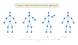
The compact representation allows motion diffusion models to generate 4-second sequences in under one second on a single GPU, a stark contrast to the minutes required for pixel-space video generation. However, rendering the skeletal motion as a photorealistic video requires a separate rendering stage, often using a pretrained video diffusion model conditioned on the skeleton sequence [76][36].
Audio-Visual Generation
Videos in the real world are rarely silent: speech, music, ambient sounds, and sound effects are integral to the viewing experience. Audio-visual generation aims to produce video and audio jointly, or to condition one modality on the other.
The core architectural idea is to introduce cross-modal attention between audio and video representations within the diffusion backbone. Let be the video latent and be the audio spectrogram latent (where is the number of audio frames and is the frequency dimension). Cross-modal attention computes: (AV QKV) where are learned projection matrices. This allows the video denoiser to attend to audio features at each denoising step, aligning visual events with their corresponding sounds.
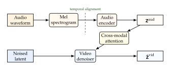
Ruan et al. [77] demonstrated that a joint audio-video diffusion model (MM-Diffusion) can generate coherent audio-video pairs by running coupled diffusion processes in both modalities, with cross-attention providing the synchronisation signal. The key challenge is temporal alignment: a drum hit at time in the audio must correspond to the visual impact at the same time in the video. This is typically enforced through positional encoding that shares a common time axis across modalities.
Talking Head Synthesis
Talking head synthesis generates a video of a person speaking, driven by an audio clip, a text transcript, or both. The output must satisfy three simultaneous constraints: (i) lip movements must be synchronised with the audio, (ii) facial expressions must be natural and emotionally appropriate, and (iii) the identity of the person must remain consistent across all frames.
Facial Action Unit Conditioning
Many talking-head models condition on facial action units (AUs), a standardised encoding of facial muscle activations derived from the Facial Action Coding System (FACS). Each AU corresponds to a specific muscle group (e.g., AU1 = inner brow raiser, AU12 = lip corner puller). A vector of AU intensities (where is the number of tracked AUs, typically 17–46) provides a compact, disentangled representation of facial expression that can be extracted from audio using a learned mapping.
Lip Synchronisation Loss
A critical component of talking-head quality is lip-audio synchronisation. The standard approach uses a pretrained sync expert network that takes a short video clip (typically 5 frames centred on the mouth region) and the corresponding audio segment, and outputs a synchronisation score . The five-frame window is only defined for centre frames that have two neighbours on each side, so the loss is averaged over (there are such frames, assuming ): (SYNC LOSS) Implementations that prefer to score all frames replicate the first and last frame (and the corresponding audio) twice, so that the window is defined for every ; the sum then runs over with the normaliser . The two conventions differ only in how the four boundary frames are weighted.
EMO [78] and AniPortrait [79] represent the current state of the art in diffusion-based talking-head synthesis. EMO introduces a speed controller and a face region controller that allow fine-grained control over the dynamics and spatial extent of facial animations. AniPortrait uses a two-stage pipeline: first generating a sequence of facial landmarks from audio, then rendering those landmarks into a photorealistic video using a diffusion-based image animator.
Remark 96 (Identity preservation).
A persistent challenge in talking-head synthesis is maintaining the subject's identity across frames and across different driving signals. The model must learn to separate identity (which should remain constant) from expression and pose (which should change). This is typically achieved through identity embedding networks that extract a fixed identity vector from a reference image and inject it into the denoiser via cross-attention or adaptive normalisation.
Virtual Try-On
Virtual try-on generates images or videos of a person wearing a specified garment, given a reference image of the person and a flat-lay image of the garment. The diffusion-based approach conditions the generation on a warped garment obtained through appearance flow estimation.
Definition 88 (Appearance Flow for Virtual Try-On).
Let be the garment image and be the person image. An appearance flow network estimates a dense deformation field that warps the garment to align with the person's pose: (Garment WARP) where denotes spatial warping via bilinear sampling, as in (WARP Error). The warped garment is then used as a conditioning input to the diffusion model, which refines the warped result into a photorealistic composite.
For video virtual try-on, the warping must be temporally coherent: the garment must deform smoothly as the person moves. This is achieved by extending the appearance flow to a spatiotemporal field and adding a temporal smoothness regulariser: (FLOW Smooth)
DreamPose [80] demonstrates that a pretrained image diffusion model can be adapted for fashion video generation by conditioning on pose sequences extracted from a driving video. CatVTON [81] simplifies the pipeline by using concatenation-based conditioning, directly concatenating the garment image with the noised person image along the channel dimension, eliminating the need for a separate warping network.
Connections and Synthesis
Video diffusion models do not exist in isolation. They draw upon, extend, and illuminate ideas from nearly every major topic covered in this book. In this section, we make these connections explicit, linking the techniques developed throughout this chapter to the theoretical foundations established in earlier parts. Each connection is presented as an insight box that identifies the specific relationship and points to the relevant chapter for further study.
Variational Inference
Insight.
The video VAE as a variational model (8). The video autoencoder at the heart of latent video diffusion is a variational autoencoder in the precise sense developed in 8. The encoder parameterises an approximate posterior , the decoder parameterises the likelihood , and training maximises the evidence lower bound: (Video VAE ELBO) The video-specific challenge is that is a high-dimensional spatiotemporal tensor, so the KL regularisation must balance spatial and temporal compression. The causal VAE architectures discussed in earlier sections ensure that the posterior factorises appropriately for autoregressive generation.
Optimal Transport and Flow Matching
Insight.
Flow matching as optimal transport (14). The flow matching framework, increasingly preferred over the classical DDPM formulation for video generation, has deep roots in optimal transport theory. Following the convention of Definition 49 (, ), the conditional flow path is a straight segment between data at and noise at ; sampling integrates it in reverse. A straight segment traversed at constant speed is exactly the geodesic of the Benamou–Brenier dynamical formulation of optimal transport, which is where the connection to 14 enters.
The connection must, however, be stated carefully, because it is routinely overstated. What is straight is each conditional path, one pair at a time. The field the model actually learns is the marginal velocity , an average over all pairs that pass through at time . Under the standard independent coupling this averaged field is in general not a gradient field, so there is no Kantorovich potential whose gradient it is, and the map it induces from noise to data is in general not the Monge map: paths that cross are averaged into a field whose integral curves do not cross, and the resulting coupling is not the optimal one. The identification of the learned field with of a convex Kantorovich potential - Brenier's theorem - holds only when the training pairs are drawn from an optimal coupling, as in OT-coupled and minibatch-OT flow matching, or approximately after rectification (Theorem 7). What survives without any such assumption, and what actually matters in practice, is the curvature claim: linear conditional paths give a marginal field whose integral curves are far straighter than the curved probability-flow trajectories of DDPM, and straighter trajectories tolerate coarser Euler discretisation - hence fewer sampling steps.
Insight.
FVD is the Wasserstein distance (14, 4). As we proved in Theorem 11, the Fréchet Video Distance is exactly the squared -Wasserstein distance between Gaussians fitted to the real and generated feature distributions. This connects the evaluation of video generation models directly to the theory of optimal transport. The Wasserstein distance has several properties that make it a natural choice for comparing generative distributions: it metrises weak convergence, it is well-defined even when the supports of the two distributions do not overlap (unlike KL divergence), and it has a geometric interpretation as the minimum-cost transport plan.
Generative Adversarial Networks
Insight.
Adversarial losses in video autoencoders (9). The training of video autoencoders often includes an adversarial component, a discriminator that distinguishes real from reconstructed video patches. This use of adversarial training within a diffusion pipeline creates a direct connection to the GAN framework of 9. The discriminator loss provides a learned perceptual metric that penalises high-frequency artifacts that reconstruction losses (MSE, LPIPS) might miss. Historically, GANs were the dominant paradigm for video generation before diffusion models, with MoCoGAN, DVD-GAN, and StyleGAN-V pushing the boundaries of resolution and temporal coherence. The transition to diffusion brought improved training stability and diversity at the cost of increased sampling time, a tradeoff that distillation techniques (discussed in earlier sections) are steadily resolving.
Memory and Long-Context Processing
Insight.
KV-cache and sparse attention for long video (24). Generating videos longer than a few seconds requires processing context windows that span hundreds or thousands of latent frames. The memory management techniques developed in 24, including KV-cache compression, sliding window attention, and retrieval-augmented generation, are directly applicable. The temporal caching strategies discussed in earlier sections (where attention outputs from previous denoising steps are reused for distant frames) are a video-specific instantiation of the KV-cache eviction policies developed for long-context language models. Similarly, the hierarchical attention patterns used in video DiTs (local windows for nearby frames, global tokens for distant ones) mirror the sparse attention architectures designed for processing long documents.
Continual Learning
Insight.
Adapting video models without forgetting (26). Video diffusion models are typically pretrained on massive datasets and then fine-tuned for specific domains (e.g., medical imaging, autonomous driving, artistic styles). This fine-tuning must avoid catastrophic forgetting of the general video generation capabilities learned during pretraining. The continual learning framework of 26 provides the theoretical tools: elastic weight consolidation (EWC) identifies which parameters are critical for existing capabilities, LoRA and adapter layers add new capabilities with minimal parameter interference, and experience replay maintains a buffer of pretraining examples to prevent distribution shift. The LoRA-based fine-tuning approach used in AnimateDiff and similar systems is precisely a low-rank adaptation strategy designed to minimise forgetting.
Agentic AI and World Models
Insight.
Video diffusion as a world model for planning (26, agentic AI). A video diffusion model trained on large-scale video data implicitly learns a world model: given a current state (the first frame or a text description) and an action (a camera movement, a text instruction, or a control signal), it can simulate the future evolution of the scene. This capability connects directly to the world model paradigm in reinforcement learning [58], where an agent plans by “imagining” future trajectories in a learned simulator. Recent work such as Genie [52], UniSim [50], and Cosmos [59] has begun to exploit this connection, using video diffusion models as the dynamics model in model-based RL. The key challenge is that diffusion sampling is stochastic: the model generates plausible futures rather than deterministic predictions, which requires planning algorithms that can reason over distributions of outcomes rather than point estimates.
Normalizing Flows
Insight.
Flow matching bridges diffusion and normalizing flows (18). The flow matching formulation of video diffusion models can be viewed as a continuous normalizing flow (CNF) with a specific parameterisation of the velocity field. In 18, we studied normalizing flows as invertible transformations that map a simple base distribution to the data distribution, with the log-likelihood computed via the change-of-variables formula. Flow matching simplifies this by abandoning exact invertibility and exact likelihood in favour of a simulation-free training objective. The resulting model defines a probability flow ODE whose trajectories transport noise to data, just as in a CNF, but the training is dramatically simpler because it avoids the expensive Jacobian computation required for exact likelihood. This theoretical connection explains why flow matching has displaced both DDPM and classical normalizing flows in modern video generation systems.
Neural Network Engineering
Insight.
RoPE, MoE, and distillation (28). Video diffusion models are among the largest and most computationally demanding neural networks in existence, and they benefit enormously from the engineering techniques catalogued in 28. Rotary positional embeddings (RoPE), extended to 3D for spatiotemporal position encoding, enable resolution-flexible generation without retraining. Mixture-of-experts (MoE) layers allow the model to scale capacity without proportionally scaling computation, activating only a subset of experts for each token. Distillation techniques (progressive distillation, consistency distillation, adversarial distillation) compress the sampling process from dozens of steps to one or a few, bringing video generation closer to real-time. Each of these techniques is developed from first principles in 28 and finds direct application in the video diffusion architectures discussed throughout this chapter.
Connections Map
Figure 42 visualises the connections between video diffusion and the other topics covered in this book.
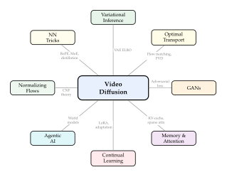
Open Problems and Future Directions
Despite the remarkable progress documented in this chapter, video diffusion models remain far from the ideal video generation system envisioned in our desiderata (The video generation desiderata). In this section, we identify five fundamental open problems that define the frontier of the field. For each problem, we provide a formal statement, discuss why it is hard, and outline promising directions of attack.
Open Problem 1: Real-Time Generation
Current state-of-the-art video diffusion models require minutes to generate a few seconds of video on high-end GPUs. Interactive applications (video games, virtual reality, live communication) require generation at or near the video frame rate, which for standard video means 24–60 frames per second.
Conjecture 1 (Real-Time Video Diffusion).
There exists an architecture and a sampling procedure such that:
processes a video latent in time (linear in the latent volume);
requires function evaluations to produce output within of the full-step quality (measured in FVD);
the combined pipeline generates video at fps on a single consumer GPU with GB of memory.
Achieving this conjecture requires roughly a speedup over current systems, which must come from a combination of sources:
Architectural efficiency: Replacing quadratic attention with linear-time alternatives (state-space models, linear attention, sparse attention patterns) could reduce the per-step cost by – for long videos.
Fewer sampling steps: Consistency distillation, adversarial distillation, and rectified flow already reduce the step count from 50–100 to 1–4, providing a – speedup.
Temporal caching: Reusing attention maps and intermediate activations across nearby frames can reduce the effective number of full network evaluations by –.
Hardware specialisation: Custom accelerators designed for the specific computation patterns of diffusion models (e.g., streaming denoising with pipelined attention) could provide an additional – improvement.
The product of these factors () suggests that the conjecture is not obviously impossible, but each factor is at the optimistic end of current estimates.
Open Problem 2: Minute-Scale Temporal Consistency
Generating videos longer than 10–15 seconds with consistent characters, environments, and narratives remains extremely challenging. Current approaches use autoregressive chunking (where each new chunk is conditioned on the end of the previous one), but this introduces accumulated drift: small inconsistencies compound over time, leading to “identity morphing” where characters gradually change appearance, and “environment shifting” where backgrounds drift between shots.
Problem 1 (Minute-Scale Consistency).
Design a video generation system that produces -frame videos (with corresponding to at least 60 seconds at 24 fps, i.e., ) such that:
Subject identity is preserved throughout: for all , where measures identity similarity;
Background consistency is maintained: for all and ;
Narrative coherence is preserved: actions initiated in early frames are completed in later frames in a causally consistent manner.
This problem is fundamentally difficult because it requires the model to maintain a persistent “world state” across a context window that is orders of magnitude larger than current training clip lengths. Promising approaches include:
Hierarchical planning: first generating a coarse storyboard at low temporal resolution, then filling in details at full resolution conditioned on the storyboard;
Persistent memory modules: maintaining an explicit memory bank of character appearances, object states, and scene layouts that is queried and updated throughout generation;
Test-time optimisation: periodically optimising the generation to enforce consistency constraints (identity matching, background alignment) between distant frames.
Open Problem 3: Physical Grounding
Current video diffusion models learn an implicit model of physics from training data: they produce videos where objects usually fall downward, water usually flows downhill, and rigid bodies usually maintain their shape. However, they have no explicit physical constraints and routinely produce physically impossible outputs (objects that pass through each other, fluids that flow upward, shadows that are inconsistent with the light source).
Problem 2 (Physics-Constrained Diffusion).
Let be a differentiable operator that encodes physical constraints (e.g., conservation laws, Navier–Stokes equations, rigid-body dynamics). A video satisfies the physics if . Design a video diffusion model such that (Physics Constraint) i.e., the model generates only physically valid videos.
This problem sits at the intersection of generative modelling and physics-informed machine learning. The difficulty is twofold: (i) the physical constraints are defined in pixel space (or a physical state space) but the diffusion process operates in latent space, so the constraints must be “lifted” through the decoder; and (ii) hard constraints on the support of a learned distribution are fundamentally harder to enforce than soft penalties in the loss function.
Possible approaches include:
Guided sampling: Using a differentiable physics simulator as a guidance function during the denoising process, steering the trajectory toward physically valid outputs at each step;
Constrained latent spaces: Training the video autoencoder such that its latent space inherently respects physical constraints (e.g., by training with a physics-based reconstruction loss);
Hybrid architectures: Combining a neural diffusion model (for appearance) with a symbolic physics engine (for dynamics), generating the physical state trajectory first and then rendering it into video.
Open Problem 4: Compositional Generation
Generating videos with multiple interacting objects, each with distinct attributes and behaviours, remains a significant weakness of current models. A prompt such as “a red ball bounces off a blue cube while a green sphere rolls in from the left” requires the model to:
correctly instantiate three distinct objects;
assign the correct colour to each;
animate each object with physically plausible motion;
model the interaction (the bounce) between the ball and cube;
maintain the identity and attributes of each object throughout the video.
Current models frequently fail at one or more of these sub-tasks, exhibiting attribute leakage (the red ball becomes blue), object merging (two objects fuse into one), or interaction failure (the ball passes through the cube).
Problem 3 (Compositional Video Generation).
Given a structured scene description specifying objects with attributes (colour, shape, texture) and motions (trajectory, dynamics), generate a video such that:
Each object appears in the video with attributes ;
Each object follows motion unless modified by interactions;
Pairwise interactions between objects are physically plausible;
Object identities and attributes are maintained throughout.
Compositional generation requires the model to maintain a form of object-centric representation within the diffusion process, a capability that monolithic architectures do not naturally support. Promising directions include slot-based diffusion models (where each object has its own latent “slot” that interacts with other slots through learned dynamics), layout-conditioned generation (where bounding boxes or segmentation masks constrain where each object appears), and compositional score functions (where the score for a multi-object scene is decomposed into per-object scores that are combined at inference time).
Open Problem 5: Unified Multimodal Generation
The ultimate vision for generative AI is a single model that can produce any combination of modalities: video with synchronised audio and subtitles, 3D scenes that can be explored from any viewpoint, and interactive environments that respond to user actions. Current systems treat each modality (video, audio, text, 3D) with separate models or separate heads, limiting the coherence of cross-modal outputs.
Problem 4 (Unified Multimodal Generation).
Design a single generative model over a joint space such that:
Marginal generation in any single modality matches or exceeds specialist models;
Conditional generation across modalities (e.g., textvideo, videoaudio, video3D) is coherent;
Joint generation of all modalities simultaneously produces consistent outputs (e.g., a 3D scene that, when rendered from any viewpoint, produces video with correct audio).
This is perhaps the most ambitious open problem in generative AI. Progress will likely require:
A unified tokenisation scheme that maps all modalities into a shared latent space;
A shared backbone architecture (likely a transformer) that can process tokens from all modalities with appropriate inductive biases for each;
Training procedures that balance the learning signals from different modalities, preventing any single modality from dominating;
Evaluation frameworks that measure cross-modal consistency, not just per-modal quality.
Key Idea.
The next frontier. The five open problems above trace an arc from engineering (real-time generation) through science (physical grounding, compositionality) to a grand unified vision (multimodal generation). Progress on each problem feeds into the others: faster models enable longer videos, physical grounding improves compositionality, compositionality enables richer multimodal scenes, and the ability to generate coherent multimodal outputs opens up new applications that demand all of the above. Solving these problems will require not just better neural networks, but deeper integration of generative modelling with physics, perception, and reasoning.
Exercises
Exercise 51 (Video Forward Process).
Consider a video latent and the standard DDPM forward process with noise schedule .
Derive the marginal distribution by showing that (EX Forward) where the noise has the same shape as . Hint: The forward process factorises independently across all spatial and temporal dimensions.
Show that the noise added to frame is independent of the noise added to frame for . Formally, show that the conditional distribution , where denotes the -th frame of .
Explain why this frame-wise noise independence is important for the design of the denoiser: if the noise is independent across frames, all inter-frame correlations in come from the signal component , and the denoiser must learn to exploit these correlations.
At what noise level does the inter-frame correlation become negligible? Express your answer in terms of and the inter-frame correlation coefficient .
Exercise 52 (Factored Attention Complexity).
Consider a video latent of shape , where is the number of spatial tokens per frame and is the number of temporal tokens per spatial position.
Compute the FLOPs of full spatiotemporal attention over all tokens. Express your answer in terms of and the head dimension .
Compute the FLOPs of factored attention, where spatial attention is applied independently to each frame (cost ) and temporal attention is applied independently to each spatial position (cost ).
Find the ratio of factored to full attention FLOPs. Under what condition on , , is factored attention most advantageous?
For a typical configuration of , , , and head dimension , compute the actual FLOP ratio and estimate the wall-clock speedup assuming perfect parallelism.
Suppose you have a fixed total token budget . Find the “optimal aspect ratio” that minimises the total factored attention FLOPs, subject to . Hint: Use the AM-GM inequality.
Exercise 53 (Causal Convolution Receptive Field).
Consider a stack of causal 1D convolutional layers along the temporal axis, each with kernel size and dilation factor for layer .
Show that the temporal receptive field of the stack is (EX Receptive)
For the common choice of exponentially increasing dilation , simplify the expression and show that .
How many layers are needed to achieve a receptive field of frames with and exponential dilation? Note that with the formula in part (b) reduces to , so the attainable receptive fields are exactly ; a target such as has no integer solution, and the smallest stack that covers it has ().
Compare this to the receptive field of a single temporal self-attention layer. What is the fundamental advantage of attention over convolution for temporal modelling?
What is the advantage of causal convolution over attention for autoregressive generation? Discuss both computational cost and the ability to process variable-length inputs.
Exercise 54 (Flow Matching Path Design).
Convention. This exercise uses the flow matching time convention of Definition 49: is data and is noise. Exercise 60 below uses the DDPM convention instead ( clean, noise); the two are unrelated reparameterisations and should not be mixed within a single derivation.
Consider a conditional flow matching framework where the interpolation between noise and data follows the path: (EX FM PATH)
Derive the conditional distribution . Show that it is a Dirac delta at .
Compute the conditional velocity field and show that it equals .
Assume and are independent and fix . enumerate[label=()]
Show that the marginal law is the Gaussian-smoothed, rescaled data distribution (EX FM Marginal) i.e. a continuous mixture of Gaussians with mixing measure .
Compute its first two moments and verify that and . Note that these moments hold for any with finite second moment; they do not make Gaussian.
Show that is Gaussian if and only if is Gaussian. Hint: the “if” direction is immediate from (ii); for “only if”, write the characteristic function of as a product and invoke Cramér's decomposition theorem (if a sum of two independent random vectors is Gaussian, each summand is Gaussian).
Conclude that specifying the mean and covariance of determines only in the Gaussian case, and give a concrete non-Gaussian example - e.g. in one dimension, for which is an explicit two-component Gaussian mixture. enumerate
The marginal velocity field is defined as . Using (EX FM Marginal), write this conditional expectation explicitly as a ratio of two integrals against , and explain why it is intractable precisely because is a mixture rather than a Gaussian: were Gaussian, the conditional expectation would be affine in and available in closed form. Then explain how the flow matching training objective avoids ever computing it, by regressing on the conditional velocity of part (b) instead - and why the minimiser of that surrogate objective is nonetheless the marginal field .
Now consider a more general path with . Derive the conditional velocity field for this general path and show that the linear path is the special case , .
Exercise 55 (SNR Shift for Video).
Consider a video latent under the forward process .
The signal-to-noise ratio at time is defined as . Show that the “effective” SNR perceived by the denoiser depends on the number of tokens : when the denoiser averages information across tokens, it effectively observes for the global signal.
Explain why this means that the noise schedule designed for images () is “too easy” for video ( or more): the video denoiser sees a much higher effective SNR at the same .
The SNR-shift trick of Definition 48 addresses this by rescaling the SNR by a constant factor : . Show that the corresponding noise schedule is (EX SNR Rescale) and that in terms of the log-SNR the rescaling is the constant additive offset . Verify that (EX SNR Rescale) maps to and preserves the endpoints and .
Derive the factor for which the effective SNR of part (a) agrees between video and images at every , i.e. . Express in terms of and , and evaluate the log-SNR offset for the numbers in part (b).
A time shift is not a rescaling. It is often claimed instead that the same effect is obtained by translating the schedule in time, for a fixed . enumerate[label=()]
Show that this reproduces the constant log-SNR offset of part (c) with provided the log-SNR is affine in time, - that is, provided the schedule is exactly exponential.
Show that for a general schedule no constant works, because then depends on . Demonstrate this for the cosine schedule , whose log-SNR is : evaluate the difference at, say, with and observe that it is not constant.
Conclude that the rescaling (EX SNR Rescale), not a time translation, is the correct statement of the SNR-shift principle, and explain why the two are nonetheless often conflated. enumerate
Exercise 56 (FVD Computation).
Prove that the FVD formula ((FVD)) equals the squared -Wasserstein distance between the two fitted Gaussians. Follow these steps: enumerate[label=()]
Write the as the infimum over couplings.
Restrict to Gaussian couplings and show that the optimal coupling has correlation matrix .
Substitute and simplify to obtain the FVD formula. enumerate Hint: The theory of Gaussian optimal transport is developed in 14.
Show that FVD if and only if and .
The FVD is estimated from finite samples. Show that the bias of the sample covariance estimator introduces an additive bias in FVD, where is the feature dimension and is the sample size. This explains why large sample sizes are needed for reliable FVD estimates.
Compute the FVD between two univariate Gaussians and and verify that it simplifies to .
Exercise 57 (Temporal Caching Error Bound).
Consider a denoiser that is -Lipschitz in (i.e., for all and all ).
In the temporal caching scheme, at denoising step , the denoiser is evaluated on a subset of frames , and the output for the remaining frames is copied from the previous step .
For a cached frame , the approximate denoiser output is (the output from the previous step). Bound the approximation error in terms of and the change in the latent .
Show that the latent change between consecutive steps satisfies , where is the step size of the ODE solver.
Combining parts (a) and (b), show that the total accumulated error after denoising steps with caching fraction is bounded by . Now observe that , the fixed integration horizon of the sampler, and rewrite the bound as .
Where the trade-off is, and is not. Part (c) shows that the bound depends on the discretisation only through the product , so refining the discretisation does not, by itself, reduce the caching error at all: halving halves the per-step latent change, but doubles the number of steps at which a stale feature is reused, and the two effects cancel exactly. enumerate[label=()]
Identify the two modelling assumptions responsible for the exact cancellation. Hint: one is that the per-step error is bounded by a quantity linear in ; the other concerns whether is allowed to depend on .
Under this bound, which quantity is the dial that trades error against compute? Show that if the compute budget is the number of network evaluations, , then for fixed the bound is decreasing in the number of evaluated frames and increasing in , so the bound alone always favours the extreme .
An interior optimum in therefore requires a second error term that does improve with more steps. Name it (consider the ODE solver's own discretisation error, which for Euler is per step) and write down the combined bound. Sketch how an interior optimum arises once both terms are present and the compute budget is held fixed. enumerate
In practice, temporal caching uses a “stale-by-one” scheme where every other frame is cached. Argue informally that for natural videos (where the denoiser output varies smoothly across nearby frames), the actual error is much smaller than the worst-case Lipschitz bound.
Exercise 58 (Camera Conditioning with Plücker Coordinates).
A ray in 3D space can be parameterised by its origin and direction (with ). The Plücker coordinates of this ray are the pair where is the moment.
Show that the moment is independent of the choice of origin point on the ray: if is another point on the ray, then .
The reciprocal product, with its hypothesis. Assume first that the two rays are not parallel, . Show that the lines they span intersect if and only if the reciprocal product vanishes: . Hint: express both lines in parametric form, impose the intersection condition, and use the identity .
Why the hypothesis is needed. Now suppose for a scalar . Show that the reciprocal product vanishes identically, whatever and are. Hint: for every . Conclude that the test reports “intersecting” for every pair of parallel lines, including distinct parallel lines that never meet, so the “if and only if” of part (b) is false without the non-parallelism hypothesis. Explain why this degenerate case matters in practice for camera conditioning: rays from a purely translating camera are very nearly parallel.
For a pinhole camera with intrinsic matrix and extrinsic matrix , derive the Plücker coordinates for the ray passing through pixel . Take care with the camera centre: if is the world-to-camera transform, so that a world point maps to , then the camera centre in world coordinates is , not . The ray direction is , normalised to unit length, and .
Explain how Plücker ray maps (one 6-channel map per frame, with channels at each pixel) provide a resolution-independent camera representation that can condition a video diffusion model.
How many degrees of freedom does a camera trajectory of frames have? How does the Plücker representation scale compared to simply providing camera matrices?
Exercise 59 (Autoregressive Chunk Overlap).
Consider generating a long video by autoregressively generating chunks of frames each, with an overlap of frames between consecutive chunks, for a target length of total frames. The overlap frames serve as conditioning context for the next chunk. This is the notation of Definition 71: is the chunk size and the total, not the other way round.
How many chunks are needed to generate a video of total frames? Express in terms of , , and , and check your answer against (AR Chunk).
The total number of denoised frames (counting overlaps) is . Compute the “overhead ratio” and show that it approaches for large . Evaluate it for , , .
Consider the consistency of the overlap region. If the diffusion model's denoiser has variance per pixel in the generated output, argue that the mismatch between the end of chunk and the beginning of chunk (in the overlap region) has expected squared error per pixel when the overlap is averaged. State the independence assumption this argument needs, and say why it is at best approximate here.
In practice, the overlap is not averaged but rather the previous chunk's overlap frames are used as a conditioning signal (e.g., through inpainting or latent blending). Discuss the qualitative difference between these two approaches in terms of consistency and diversity.
Show that in the limiting case - which Definition 71 explicitly excludes, requiring - the inter-chunk boundary has no conditioning signal, and the video is essentially independent clips. What is the minimum needed for reasonable consistency? Justify your answer with a simple perceptual argument.
Exercise 60 (Consistency Distillation for Video).
Convention. This exercise uses the DDPM time convention of Definition 53: is the clean latent and is pure noise. This is the opposite orientation to Exercise 54.
Consistency models [60] learn a function that maps any point on the diffusion trajectory to the trajectory's origin . The key property is self-consistency: for any on the same trajectory.
Write the consistency distillation loss for a pretrained teacher denoiser : (EX CD LOSS) where is obtained by taking one ODE step from using the teacher, and denotes the EMA (exponential moving average) of the student parameters.
Explain the role of the EMA target . Why is it important not to use the same parameters for both the student and the target? Hint: Consider what happens when the target is non-stationary.
For video generation, the consistency function must be applied to the full video latent . Discuss the computational challenge and propose a strategy for applying consistency distillation to video transformers.
After distillation, generation requires only a single forward pass: where . What is the theoretical quality loss compared to the full multi-step teacher? Express this in terms of the distillation loss and the number of discretisation steps used during distillation.
Exercise 61 (LoRA Rank Selection for Video Models).
Consider a video diffusion transformer with attention layers, each containing four weight matrices () of shape where . LoRA [40] adapts each weight matrix by adding a low-rank update where is the down-projection and is the up-projection. Following Hu et al., the down-projection is initialised from a Gaussian and the up-projection is initialised to zero, so that at the start of training and the adapted model begins exactly at the base model.
Compute the number of trainable LoRA parameters for ranks when LoRA is applied to all four matrices in all layers. Express each as a fraction of the total model parameters (which are approximately for the attention layers alone).
The expressiveness of a rank- LoRA update is bounded by the rank: . Argue that for a fine-tuning task that requires modifying singular values of , we need .
In practice, video fine-tuning tasks (e.g., adapting a general model to generate anime-style videos) typically require rank –. Explain intuitively why this is much less than : what does this imply about the dimensionality of the “style subspace”?
Compare the training memory requirements for full fine-tuning versus LoRA with . Account for both the parameter memory and the optimiser state memory (assuming Adam, which stores first and second moments for each trainable parameter).
LoRA modules can be merged back into the base model after fine-tuning: . Discuss whether multiple LoRA adaptations (e.g., one for style, one for motion) can be composed. Under what conditions does composition work well, and when does it fail?
Exercise 62 (World Model Planning).
(Research exercise.) This exercise asks you to think beyond the material covered in the chapter. There is no single correct answer; the goal is to develop and justify a concrete proposal.
A video diffusion model trained on large-scale video data implicitly learns a “world model”: given a current visual state and an action, it can “imagine” the future state by generating continuation frames [6][58].
Propose a framework for using a pretrained video diffusion model as the dynamics model in a model-based reinforcement learning agent. Your framework should specify: enumerate[label=()]
How the current observation is encoded into the diffusion model's latent space;
How actions are injected as conditioning signals;
How future rewards are estimated from the generated video;
How the stochasticity of diffusion sampling is handled in the planning algorithm. enumerate
Identify three fundamental limitations of using a video diffusion model as a world model compared to a dedicated dynamics model (e.g., a learned physics simulator). For each limitation, propose a mitigation strategy.
One approach is to use the diffusion model for “imagination” (generating candidate future trajectories) and a separate value network for evaluation. Write the planning objective: (EX Planning) where is the conditional video distribution given the current frame and action , and is the value function. Discuss how to estimate this expectation efficiently using a small number of generated trajectories.
Recent systems such as Genie [52] and UniSim [50] have demonstrated interactive video generation conditioned on user actions. Read one of these papers and summarise (in 1–2 paragraphs) how it addresses the challenges you identified in part (b).
Key Idea.
The arc of video diffusion. This chapter has traced the complete arc of video diffusion models, from the foundational challenge of generating coherent spatiotemporal content to the cutting-edge systems that produce high-definition clips of roughly ten seconds from a text prompt. Minute-scale generation with stable identity and narrative is not a solved problem, and is stated as such in Problem 1. The key ideas form a layered stack. At the bottom, video autoencoders compress the raw pixel tensor into a compact latent space, making diffusion tractable. Above that, spatiotemporal architectures (3D U-Nets, Video DiTs) interleave spatial and temporal attention to model both appearance and motion. Conditioning mechanisms (text, image, camera, motion) give users fine-grained control over the generated content. Efficient sampling strategies (distillation, caching, progressive generation) reduce the computational cost from minutes to seconds. Training at scale (curriculum learning, mixed-resolution batching, multi-stage pipelines) enables the massive data and compute investments needed for frontier models. And evaluation metrics (FVD, VBench, human evaluation) provide the yardstick by which progress is measured.
At its core, the entire enterprise rests on a single mathematical idea: learning to reverse a noise process, one step at a time, guided by the statistics of natural video. That this simple idea, when combined with massive scale and careful engineering, can produce videos that are increasingly indistinguishable from reality is one of the most remarkable achievements of modern machine learning. The open problems identified in this chapter suggest that the story is far from over: real-time generation, minute-scale consistency, physical grounding, compositional control, and unified multimodal synthesis remain grand challenges that will drive the field for years to come.
References
-
Stochastic Video Generation with a Learned Prior
BibTeX
@article{denton2018stochastic, title={Stochastic Video Generation with a Learned Prior}, author={Denton, Emily and Fergus, Rob}, journal={International Conference on Machine Learning}, year={2018} }Journal article
-
VideoGPT: Video Generation using VQ-VAE and Transformers
BibTeX
@article{yan2021videogpt, title={{VideoGPT}: Video Generation using {VQ-VAE} and Transformers}, author={Yan, Wilson and Zhang, Yunzhi and Abbeel, Pieter and Srinivas, Aravind}, journal={arXiv preprint arXiv:2104.10157}, year={2021} }Journal article
-
Video Diffusion Models
BibTeX
@article{ho2022video, title={Video Diffusion Models}, author={Ho, Jonathan and Salimans, Tim and Gritsenko, Alexey and Chan, William and Norouzi, Mohammad and Fleet, David J.}, journal={Advances in Neural Information Processing Systems}, volume={35}, year={2022} }Journal article
-
Make-A-Video: Text-to-Video Generation without Text-Video Data
BibTeX
@article{singer2022make, title={{Make-A-Video}: Text-to-Video Generation without Text-Video Data}, author={Singer, Uriel and Polyak, Adam and Hayes, Thomas and Yin, Xi and An, Jie and Zhang, Songyang and Hu, Qiyuan and Yang, Harry and Ashual, Oron and Gafni, Oran and others}, journal={International Conference on Learning Representations}, year={2023} }Journal article
-
Imagen Video: High Definition Video Generation with Diffusion Models
BibTeX
@article{ho2022imagen, title={Imagen Video: High Definition Video Generation with Diffusion Models}, author={Ho, Jonathan and Chan, William and Saharia, Chitwan and Whang, Jay and Gao, Ruiqi and Gritsenko, Alexey and Kingma, Diederik P. and Poole, Ben and Norouzi, Mohammad and Fleet, David J. and Salimans, Tim}, journal={arXiv preprint arXiv:2210.02303}, year={2022} }Journal article
-
Video Generation Models as World Simulators
BibTeX
@article{brooks2024sora, title={Video Generation Models as World Simulators}, author={Brooks, Tim and Peebles, Bill and Holmes, Connor and DePue, Will and Guo, Yufei and Jing, Li and Schnurr, David and Taylor, Joe and Luhman, Troy and Luhman, Eric and others}, journal={OpenAI Technical Report}, year={2024} }Journal article
-
Wan: Open and Advanced Large-Scale Video Generative Models
BibTeX
@article{wang2025wan, ids={wan2025wan}, title={{Wan}: Open and Advanced Large-Scale Video Generative Models}, author={Wang, Ang and Guo, Baole and Liang, Bin and Luo, Bing and Chen, Biao and others}, journal={arXiv preprint arXiv:2503.20314}, year={2025} }Journal article
-
Stable Video Diffusion: Scaling Latent Video Diffusion Models to Large Datasets
BibTeX
@article{blattmann2023stable, title={Stable Video Diffusion: Scaling Latent Video Diffusion Models to Large Datasets}, author={Blattmann, Andreas and Dockhorn, Tim and Kulal, Sumith and Mendelevitch, Daniel and Kilian, Maciej and Lorber, Dominik and Levi, Yam and English, Zion and Voleti, Vikram and Letts, Adam and others}, journal={arXiv preprint arXiv:2311.15127}, year={2023} }Journal article
-
Scalable Diffusion Models with Transformers
BibTeX
@inproceedings{peebles2023scalable, title={Scalable Diffusion Models with Transformers}, author={Peebles, William and Xie, Saining}, booktitle={Proceedings of the IEEE/CVF International Conference on Computer Vision}, year={2023} }Conference paper
-
Denoising Diffusion Implicit Models
BibTeX
@article{song2020denoising, title={Denoising Diffusion Implicit Models}, author={Song, Jiaming and Meng, Chenlin and Ermon, Stefano}, journal={International Conference on Learning Representations}, year={2021} }Journal article
-
FlashAttention: Fast and Memory-Efficient Exact Attention with IO-Awareness
BibTeX
@inproceedings{dao2022flashattention, title={Flash{A}ttention: Fast and Memory-Efficient Exact Attention with {IO}-Awareness}, author={Dao, Tri and Fu, Daniel Y. and Ermon, Stefano and Rudra, Atri and R{\'e}, Christopher}, booktitle={Advances in Neural Information Processing Systems}, volume={35}, year={2022} }Conference paper
-
Auto-Encoding Variational Bayes
BibTeX
@inproceedings{kingma2013auto, title={Auto-Encoding Variational {B}ayes}, author={Kingma, Diederik P and Welling, Max}, booktitle={International Conference on Learning Representations}, year={2014} }Conference paper
-
Neural Discrete Representation Learning
BibTeX
@article{van2017neural, title={Neural Discrete Representation Learning}, author={van den Oord, Aaron and Vinyals, Oriol and Kavukcuoglu, Koray}, journal={Advances in Neural Information Processing Systems}, year={2017} }Journal article
-
High-resolution image synthesis with latent diffusion models
BibTeX
@article{rombach2022high, title={High-resolution image synthesis with latent diffusion models}, author={Rombach, Robin and Blattmann, Andreas and Lorenz, Dominik and Esser, Patrick and Ommer, Bj{\"o}rn}, journal={Proceedings of the IEEE/CVF Conference on Computer Vision and Pattern Recognition}, pages={10684--10695}, year={2022} }Journal article
-
MAGVIT: Masked Generative Video Transformer
BibTeX
@article{yu2023magvit, title={{MAGVIT}: Masked Generative Video Transformer}, author={Yu, Lijun and Cheng, Yong and Sohn, Kihyuk and Lezama, Jos{\'e} and Zhang, Han and Chang, Huiwen and Hauptmann, Alexander G. and Yang, Ming-Hsuan and Hao, Yuan and Essa, Irfan and others}, journal={Conference on Computer Vision and Pattern Recognition}, year={2023} }Journal article
yu2023language
-
CogVideoX: Text-to-Video Diffusion Models with An Expert Transformer
BibTeX
@article{yang2024cogvideox, title={{CogVideoX}: Text-to-Video Diffusion Models with An Expert Transformer}, author={Yang, Zhuoyi and Teng, Jiayan and Zheng, Wendi and Ding, Ming and Huang, Shiyu and Xu, Jiazheng and Yang, Yuanming and Hong, Wenyi and Zhang, Xiaohan and Feng, Guanyu and others}, journal={arXiv preprint arXiv:2408.06072}, year={2024} }Journal article
zheng2024open
-
Spectral normalization for generative adversarial networks
BibTeX
@inproceedings{miyato2018spectral, title={Spectral normalization for generative adversarial networks}, author={Miyato, Takeru and Kataoka, Toshiki and Koyama, Masanori and Yoshida, Yuichi}, booktitle={Proceedings of the International Conference on Learning Representations}, year={2018}, url={https://openreview.net/forum?id=B1QRgziT-} }Conference paper
-
FiLM: Visual Reasoning with a General Conditioning Layer
BibTeX
@article{perez2018film, title={{FiLM}: Visual Reasoning with a General Conditioning Layer}, author={Perez, Ethan and Strub, Florian and de Vries, Harm and Dumoulin, Vincent and Courville, Aaron}, journal={AAAI Conference on Artificial Intelligence}, year={2018} }Journal article
-
Latte: Latent Diffusion Transformer for Video Generation
BibTeX
@article{ma2024latte, title={Latte: Latent Diffusion Transformer for Video Generation}, author={Ma, Xin and Wang, Yaohui and Jia, Gengyun and Chen, Xinyuan and Liu, Ziwei and Li, Yuan-Fang and Chen, Cunjian and Qiao, Yu}, journal={arXiv preprint arXiv:2401.03048}, year={2024} }Journal article
-
All are Worth Words: A ViT Backbone for Diffusion Models
BibTeX
@article{bao2023uvit, title={All are Worth Words: A {ViT} Backbone for Diffusion Models}, author={Bao, Fan and Nie, Shen and Xue, Kaiwen and Cao, Yue and Li, Chongxuan and Su, Hang and Zhu, Jun}, journal={Conference on Computer Vision and Pattern Recognition}, year={2023} }Journal article
-
On the Importance of Noise Scheduling for Diffusion Models
BibTeX
@article{chen2023simple, title={On the Importance of Noise Scheduling for Diffusion Models}, author={Chen, Ting}, journal={arXiv preprint arXiv:2301.10972}, year={2023} }Journal article
-
Scaling Rectified Flow Transformers for High-Resolution Image Synthesis
BibTeX
@inproceedings{esser2024scaling, title={Scaling Rectified Flow Transformers for High-Resolution Image Synthesis}, author={Esser, Patrick and Kulal, Sumith and Blattmann, Andreas and Entezari, Rahim and M\"{u}ller, Jonas and Saini, Harry and Levi, Yam and Lorber, Dominik and Sauer, Axel and Boesel, Frederic and others}, booktitle={Proceedings of the 41st International Conference on Machine Learning (ICML)}, year={2024} }Conference paper
-
Flow Matching for Generative Modeling
BibTeX
@inproceedings{lipman2023flow, title={Flow Matching for Generative Modeling}, author={Lipman, Yaron and Chen, Ricky T. Q. and Ben-Hamu, Heli and Nickel, Maximilian and Le, Matt}, booktitle={International Conference on Learning Representations (ICLR)}, year={2023} }Conference paper
-
Flow Straight and Fast: Learning to Generate and Transfer Data with Rectified Flow
BibTeX
@article{liu2023rectified, title={Flow Straight and Fast: Learning to Generate and Transfer Data with Rectified Flow}, author={Liu, Xingchao and Gong, Chengyue and Liu, Qiang}, journal={International Conference on Learning Representations}, year={2023} }Journal article
-
AnimateLCM: Computation-Efficient Personalized Style Video Generation without Personalized Video Data
BibTeX
@article{wang2024animatelcm, title={{AnimateLCM}: Computation-Efficient Personalized Style Video Generation without Personalized Video Data}, author={Wang, Fu-Yun and Huang, Zhaoyang and Bian, Weikang and Shi, Xiaoyu and Sun, Keqiang and Song, Guanglu and Liu, Yu and Li, Hongsheng}, journal={arXiv preprint arXiv:2402.00769}, year={2024} }Journal article
-
PAB: Pyramid Attention Broadcast for Efficient Video Generation
BibTeX
@article{zhao2024pab, title={{PAB}: Pyramid Attention Broadcast for Efficient Video Generation}, author={Zhao, Xuanlei and Zheng, Zangwei and You, Yang}, journal={arXiv preprint arXiv:2408.12588}, year={2024} }Journal article
-
Cross-Attention Makes Inference Cumbersome in Text-to-Image Diffusion Models
BibTeX
@article{zhang2024tgate, title={Cross-Attention Makes Inference Cumbersome in Text-to-Image Diffusion Models}, author={Zhang, Wentian and Liu, Haozhe and Xie, Jinheng and Faccio, Francesco and Shou, Mike Zheng and Schmidhuber, J{\"u}rgen}, journal={arXiv preprint arXiv:2404.02747}, year={2024} }Journal article
-
Progressive Distillation for Fast Sampling of Diffusion Models
BibTeX
@article{salimans2022progressive, title={Progressive Distillation for Fast Sampling of Diffusion Models}, author={Salimans, Tim and Ho, Jonathan}, journal={International Conference on Learning Representations}, year={2022} }Journal article
-
Open-Sora: Democratizing Efficient Video Production for All
BibTeX
@article{zheng2024opensora, ids={zheng2024open, opensora2024}, title={Open-{Sora}: Democratizing Efficient Video Production for All}, author={Zheng, Zangwei and Peng, Xiangyu and Yang, Tianji and Cheng, Chenhui and Wang, Shenggui and You, Yang}, journal={arXiv preprint arXiv:2412.00131}, year={2024} }Journal article
-
Movie Gen: A Cast of Media Foundation Models
BibTeX
@article{polyak2024moviegen, title={Movie {Gen}: A Cast of Media Foundation Models}, author={Polyak, Adam and Zohar, Amit and Brown, Andrew and Tjandra, Andros and Sinha, Animesh and Lee, Ann and others}, journal={arXiv preprint arXiv:2410.13720}, year={2024} }Journal article
xu2024camctrl
-
MotionCtrl: A Unified and Flexible Motion Controller for Video Generation
BibTeX
@article{wang2024motionctrl, title={{MotionCtrl}: A Unified and Flexible Motion Controller for Video Generation}, author={Wang, Zhouxia and Yuan, Ziyang and Wang, Xintao and Li, Yaowei and Chen, Tianshui and Xia, Menghan and Luo, Ping and Shan, Ying}, journal={arXiv preprint arXiv:2312.03641}, year={2024} }Journal article
deng2023drag
-
Animate Anyone: Consistent and Controllable Image-to-Video Synthesis for Character Animation
BibTeX
@article{hu2024animate, title={Animate Anyone: Consistent and Controllable Image-to-Video Synthesis for Character Animation}, author={Hu, Li and Gao, Xin and Zhang, Peng and Sun, Ke and Zhang, Bang and Bo, Liefeng}, journal={Conference on Computer Vision and Pattern Recognition}, year={2024} }Journal article
-
AnimateDiff: Animate Your Personalized Text-to-Image Diffusion Models without Specific Tuning
BibTeX
@article{guo2024animatediff, title={{AnimateDiff}: Animate Your Personalized Text-to-Image Diffusion Models without Specific Tuning}, author={Guo, Yuwei and Yang, Ceyuan and Rao, Anyi and Liang, Zhengyang and Wang, Yaohui and Qiao, Yu and Agrawala, Maneesh and Lin, Dahua and Dai, Bo}, journal={International Conference on Learning Representations}, year={2024} }Journal article
-
Exploring the Limits of Transfer Learning with a Unified Text-to-Text Transformer
BibTeX
@article{raffel2020t5, title={Exploring the Limits of Transfer Learning with a Unified Text-to-Text Transformer}, author={Raffel, Colin and Shazeer, Noam and Roberts, Adam and Lee, Katherine and Narang, Sharan and Matena, Michael and Zhou, Yanqi and Li, Wei and Liu, Peter J.}, journal={Journal of Machine Learning Research}, volume={21}, number={140}, pages={1--67}, year={2020} }Journal article
-
Learning Transferable Visual Models From Natural Language Supervision
BibTeX
@article{radford2021clip, title={Learning Transferable Visual Models From Natural Language Supervision}, author={Radford, Alec and Kim, Jong Wook and Hallacy, Chris and Ramesh, Aditya and Goh, Gabriel and Agarwal, Sandhini and Sastry, Girish and Askell, Amanda and Mishkin, Pamela and Clark, Jack and others}, journal={International Conference on Machine Learning}, year={2021} }Journal article
-
LoRA: Low-Rank Adaptation of Large Language Models
BibTeX
@article{hu2022lora, title={{LoRA}: Low-Rank Adaptation of Large Language Models}, author={Hu, Edward J and Shen, Yelong and Wallis, Phillip and Allen-Zhu, Zeyuan and Li, Yuanzhi and Wang, Shean and Wang, Lu and Chen, Weizhu}, journal={International Conference on Learning Representations}, year={2022} }Journal article
-
StreamingT2V: Consistent, Dynamic, and Extendable Long Video Generation from Text
BibTeX
@article{henschel2024streamingt2v, title={{StreamingT2V}: Consistent, Dynamic, and Extendable Long Video Generation from Text}, author={Henschel, Roberto and Khachatryan, Levon and Hayrapetyan, Daniil and Poghosyan, Hayk and Tadevosyan, Vahram and Wang, Zhangyang and Navasardyan, Shant and Shi, Humphrey}, journal={arXiv preprint arXiv:2403.14773}, year={2024} }Journal article
-
FreeNoise: Tuning-Free Longer Video Diffusion via Noise Rescheduling
BibTeX
@article{qiu2024freenoise, title={{FreeNoise}: Tuning-Free Longer Video Diffusion via Noise Rescheduling}, author={Qiu, Haonan and Weng, Menghan and Zheng, Yuxuan and Ge, Yue and Zhang, Haoji and Cai, Zhaoyang and Shan, Ying}, journal={Conference on Computer Vision and Pattern Recognition}, year={2024} }Journal article
-
NUWA-XL: Diffusion over Diffusion for eXtremely Long Video Generation
BibTeX
@article{yin2023nuwaxl, title={{NUWA-XL}: Diffusion over Diffusion for eXtremely Long Video Generation}, author={Yin, Shengming and Wu, Chenfei and Yang, Huan and Wang, Jianfeng and Wang, Xiaodong and Lei, Minheng and Duan, Nan}, journal={Association for Computational Linguistics}, year={2023} }Journal article
-
FreeInit: Bridging Initialization Gap in Video Diffusion Models
BibTeX
@article{wu2024freeinit, title={{FreeInit}: Bridging Initialization Gap in Video Diffusion Models}, author={Wu, Tianxing and Si, Chenyang and Jiang, Yuming and Huang, Ziqi and Liu, Ziwei}, journal={Conference on Computer Vision and Pattern Recognition}, year={2024} }Journal article
-
LAMP: Learn A Motion Pattern for Few-Shot Video Generation
BibTeX
@article{wu2024lamp, title={{LAMP}: Learn A Motion Pattern for Few-Shot Video Generation}, author={Wu, Ruiqi and Chen, Liangyu and Yang, Tong and Guo, Chunle and Li, Chongyi and Zhang, Xiangyu}, journal={Conference on Computer Vision and Pattern Recognition}, year={2024} }Journal article
-
TokenFlow: Consistent Diffusion Features for Consistent Video Editing
BibTeX
@article{geyer2024tokenflow, title={{TokenFlow}: Consistent Diffusion Features for Consistent Video Editing}, author={Geyer, Michal and Bar-Tal, Omer and Bagon, Shai and Dekel, Tali}, journal={International Conference on Learning Representations}, year={2024} }Journal article
-
Pix2Video: Video Editing using Image Diffusion
BibTeX
@article{ceylan2023pix2video, title={{Pix2Video}: Video Editing using Image Diffusion}, author={Ceylan, Duygu and Huang, Chun-Hao Paul and Mitra, Niloy J.}, journal={International Conference on Computer Vision}, year={2023} }Journal article
-
FateZero: Fusing Attentions for Zero-shot Text-based Video Editing
BibTeX
@article{qi2023fatezero, title={{FateZero}: Fusing Attentions for Zero-shot Text-based Video Editing}, author={Qi, Chenyang and Cun, Xiaodong and Zhang, Yong and Lei, Chenyang and Wang, Xintao and Shan, Ying and Chen, Qifeng}, journal={International Conference on Computer Vision}, year={2023} }Journal article
-
Rerender A Video: Zero-Shot Text-Guided Video-to-Video Translation
BibTeX
@article{yang2023rerender, title={Rerender A Video: Zero-Shot Text-Guided Video-to-Video Translation}, author={Yang, Shuai and Zhou, Yifan and Liu, Ziwei and Loy, Chen Change}, journal={ACM SIGGRAPH Asia}, year={2023} }Journal article
-
UniSim: Learning Interactive Real-World Simulators
BibTeX
@article{yang2024unisim, title={{UniSim}: Learning Interactive Real-World Simulators}, author={Yang, Mengjiao and Du, Yilun and Ghasemipour, Kamyar and Tompson, Jonathan and Schuurmans, Dale and Abbeel, Pieter}, journal={International Conference on Learning Representations}, year={2024} }Journal article
-
GameGen-X: Interactive Open-world Game Video Generation
BibTeX
@article{che2024gamegen, title={{GameGen-X}: Interactive Open-world Game Video Generation}, author={Che, Haoxuan and He, Xuanhua and Liu, Quande and Jin, Cheng and Chen, Hao}, journal={arXiv preprint arXiv:2411.00769}, year={2024} }Journal article
-
Genie: Generative Interactive Environments
BibTeX
@article{bruce2024genie, title={Genie: Generative Interactive Environments}, author={Bruce, Jake and Dennis, Michael and Edwards, Ashley and Parker-Holder, Jack and Shi, Yuge and Hughes, Edward and Lai, Matthew and Muldal, Adrien and Veloso, Theophane and others}, journal={International Conference on Machine Learning}, year={2024} }Journal article
dai2023emu
-
VideoPoet: A Large Language Model for Zero-Shot Video Generation
BibTeX
@article{kondratyuk2024videopoet, title={{VideoPoet}: A Large Language Model for Zero-Shot Video Generation}, author={Kondratyuk, Dan and Yu, Lijun and Gu, Xiuye and Lezama, Jos{\'e} and Huang, Jonathan and Hornung, Rachel and Adam, Hartwig and Akbari, Hassan and Alon, Yair and others}, journal={International Conference on Machine Learning}, year={2024} }Journal article
-
Language Model Beats Diffusion -- Tokenizer is Key to Visual Generation
BibTeX
@article{yu2024language, ids={yu2023language}, title={Language Model Beats Diffusion -- Tokenizer is Key to Visual Generation}, author={Yu, Lijun and Lezama, Jos{\'e} and Gundavarapu, Nitesh B. and Versari, Luca and Sohn, Kihyuk and Minnen, David and Cheng, Yong and Gupta, Agrim and Gu, Xiuye and Hauptmann, Alexander G. and others}, journal={International Conference on Learning Representations}, year={2024} }Journal article
-
Towards Accurate Generative Models of Video: A New Metric and Challenges
BibTeX
@article{unterthiner2019fvd, title={Towards Accurate Generative Models of Video: A New Metric and Challenges}, author={Unterthiner, Thomas and van Steenkiste, Sjoerd and Kurach, Karol and Marinier, Raphael and Michalski, Marcin and Gelly, Sylvain}, journal={arXiv preprint arXiv:1812.01717}, year={2019} }Journal article
-
VBench: Comprehensive Benchmark Suite for Video Generative Models
BibTeX
@article{huang2024vbench, title={{VBench}: Comprehensive Benchmark Suite for Video Generative Models}, author={Huang, Ziqi and He, Yinan and Yu, Jiashuo and Zhang, Fan and Si, Chenyang and Jiang, Yuming and Zhang, Yuanhan and Wu, Tianxing and Jin, Qingyang and Chanpaisit, Nattapol and others}, journal={Conference on Computer Vision and Pattern Recognition}, year={2024} }Journal article
-
World Models
BibTeX
@article{ha2018worldmodels, title={World Models}, author={Ha, David and Schmidhuber, J{\"u}rgen}, journal={arXiv preprint arXiv:1803.10122}, year={2018} }Journal article
-
Cosmos World Foundation Model Platform for Physical AI
BibTeX
@article{nvidia2025cosmos, ids={du2024cosmos}, title={Cosmos World Foundation Model Platform for Physical {AI}}, author={NVIDIA}, journal={arXiv preprint arXiv:2501.03575}, year={2025} }Journal article
-
Consistency Models
BibTeX
@article{song2023consistency, title={Consistency Models}, author={Song, Yang and Dhariwal, Prafulla and Chen, Mark and Sutskever, Ilya}, journal={International Conference on Machine Learning}, year={2023} }Journal article
-
Adding Conditional Control to Text-to-Image Diffusion Models
BibTeX
@article{zhang2023adding, title={Adding Conditional Control to Text-to-Image Diffusion Models}, author={Zhang, Lvmin and Rao, Anyi and Agrawala, Maneesh}, journal={International Conference on Computer Vision}, year={2023} }Journal article
-
Classifier-free diffusion guidance
BibTeX
@article{ho2022classifier, title={Classifier-free diffusion guidance}, author={Ho, Jonathan and Salimans, Tim}, journal={arXiv preprint arXiv:2207.12598}, year={2022} }Journal article
-
Rethinking Spatiotemporal Feature Learning: Speed-Accuracy Trade-offs in Video Classification
BibTeX
@article{xie2018rethinking, title={Rethinking Spatiotemporal Feature Learning: Speed-Accuracy Trade-offs in Video Classification}, author={Xie, Saining and Sun, Chen and Huang, Jonathan and Tu, Zhuowen and Murphy, Kevin}, journal={European Conference on Computer Vision}, year={2018} }Journal article
-
A Closer Look at Spatiotemporal Convolutions for Action Recognition
BibTeX
@article{tran2018closer, title={A Closer Look at Spatiotemporal Convolutions for Action Recognition}, author={Tran, Du and Wang, Heng and Torresani, Lorenzo and Ray, Jamie and LeCun, Yann and Paluri, Manohar}, journal={Conference on Computer Vision and Pattern Recognition}, year={2018} }Journal article
-
RoFormer: Enhanced Transformer with Rotary Position Embedding
BibTeX
@article{su2021roformer, title={{RoFormer}: Enhanced Transformer with Rotary Position Embedding}, author={Su, Jianlin and Ahmed, Murtadha and Lu, Yu and Pan, Shengfeng and Bo, Wen and Liu, Yunfeng}, journal={Neurocomputing}, volume={568}, pages={127063}, year={2024} }Journal article
-
Stochastic Interpolants: A Unifying Framework for Flows and Diffusions
BibTeX
@inproceedings{albergo2023stochastic, title={Stochastic Interpolants: A Unifying Framework for Flows and Diffusions}, author={Albergo, Michael S. and Boffi, Nicholas M. and Vanden-Eijnden, Eric}, booktitle={Proceedings of the 40th International Conference on Machine Learning (ICML)}, year={2023} }Conference paper
xing2025dynamicrafter
-
I2VGen-XL: High-Quality Image-to-Video Synthesis via Cascaded Diffusion Models
BibTeX
@article{zhang2023i2vgenxl, title={{I2VGen-XL}: High-Quality Image-to-Video Synthesis via Cascaded Diffusion Models}, author={Zhang, Shiwei and Wang, Jiayu and Zhang, Yingya and Zhao, Kang and Yuan, Hangjie and Qin, Zhiwu and Wang, Xiang and Zhao, Deli and Zhou, Jingren}, journal={arXiv preprint arXiv:2311.04145}, year={2023} }Journal article
-
Adding Conditional Control to Text-to-Image Diffusion Models
BibTeX
@article{zhang2023controlnet, title={Adding Conditional Control to Text-to-Image Diffusion Models}, author={Zhang, Lvmin and Rao, Anyi and Agrawala, Maneesh}, journal={International Conference on Computer Vision}, year={2023} }Journal article
-
DreamBooth: Fine Tuning Text-to-Image Diffusion Models for Subject-Driven Generation
BibTeX
@article{ruiz2023dreambooth, title={{DreamBooth}: Fine Tuning Text-to-Image Diffusion Models for Subject-Driven Generation}, author={Ruiz, Nataniel and Li, Yuanzhen and Jampani, Varun and Barber, Yael and Rubinstein, Michael and Aberman, Kfir}, journal={Conference on Computer Vision and Pattern Recognition}, year={2023} }Journal article
-
QLoRA: Efficient Finetuning of Quantized Language Models
BibTeX
@article{dettmers2023qlora, title={{QLoRA}: Efficient Finetuning of Quantized Language Models}, author={Dettmers, Tim and Pagnoni, Artidoro and Holtzman, Ari and Zettlemoyer, Luke}, journal={Advances in Neural Information Processing Systems}, volume={36}, year={2023} }Journal article
meng2021sdedit
-
GANs Trained by a Two Time-Scale Update Rule Converge to a Local Nash Equilibrium
BibTeX
@article{heusel2017fid, title={{GANs} Trained by a Two Time-Scale Update Rule Converge to a Local {Nash} Equilibrium}, author={Heusel, Martin and Ramsauer, Hubertus and Unterthiner, Thomas and Nessler, Bernhard and Hochreiter, Sepp}, journal={Advances in Neural Information Processing Systems}, year={2017} }Journal article
-
Quo Vadis, Action Recognition? A New Model and the Kinetics Dataset
BibTeX
@article{carreira2017i3d, title={Quo Vadis, Action Recognition? {A} New Model and the Kinetics Dataset}, author={Carreira, Jo{\~a}o and Zisserman, Andrew}, journal={Conference on Computer Vision and Pattern Recognition}, year={2017} }Journal article
-
Human Motion Diffusion Model
BibTeX
@article{tevet2023mdm, title={Human Motion Diffusion Model}, author={Tevet, Guy and Raab, Sigal and Gordon, Brian and Shafir, Yonatan and Cohen-Or, Daniel and Bermano, Amit H.}, journal={International Conference on Learning Representations}, year={2023} }Journal article
-
MagicAnimate: Temporally Consistent Human Image Animation using Diffusion Model
BibTeX
@article{xu2024magicanimate, title={{MagicAnimate}: Temporally Consistent Human Image Animation using Diffusion Model}, author={Xu, Zhongcong and Zhang, Jianfeng and Liew, Jun Hao and Yan, Hanshu and Liu, Jia-Wei and Zhang, Chenxu and Feng, Jiashi and Shou, Mike Zheng}, journal={Conference on Computer Vision and Pattern Recognition}, year={2024} }Journal article
-
MM-Diffusion: Learning Multi-Modal Diffusion Models for Joint Audio and Video Generation
BibTeX
@article{ruan2023mmdiffusion, title={{MM-Diffusion}: Learning Multi-Modal Diffusion Models for Joint Audio and Video Generation}, author={Ruan, Ludan and Ma, Yiyang and Yang, Huan and He, Huiguo and Liu, Bei and Fu, Jianlong and Yuan, Nicholas Jing and Jin, Qin and Guo, Baining}, journal={Conference on Computer Vision and Pattern Recognition}, year={2023} }Journal article
-
EMO: Emote Portrait Alive -- Generating Expressive Portrait Videos with Audio2Video Diffusion Model under Weak Conditions
BibTeX
@article{tian2024emo, title={{EMO}: Emote Portrait Alive -- Generating Expressive Portrait Videos with Audio2Video Diffusion Model under Weak Conditions}, author={Tian, Linrui and Wang, Qi and Zhang, Bang and Bo, Liefeng}, journal={European Conference on Computer Vision}, year={2024} }Journal article
-
AniPortrait: Audio-Driven Synthesis of Photorealistic Portrait Animation
BibTeX
@article{wei2024aniportrait, title={{AniPortrait}: Audio-Driven Synthesis of Photorealistic Portrait Animation}, author={Wei, Huawei and Yang, Zejun and Wang, Zhisheng}, journal={arXiv preprint arXiv:2403.17694}, year={2024} }Journal article
-
DreamPose: Fashion Video Synthesis with Stable Diffusion
BibTeX
@article{karras2023dreampose, ids={karras2024dreampose}, title={{DreamPose}: Fashion Video Synthesis with Stable Diffusion}, author={Karras, Johanna and Holynski, Aleksander and Wang, Ting-Chun and Kemelmacher-Shlizerman, Ira}, journal={International Conference on Computer Vision}, year={2023} }Journal article
-
CatVTON: Concatenation Is All You Need for Virtual Try-On with Diffusion Models
BibTeX
@article{chong2024catvton, title={{CatVTON}: Concatenation Is All You Need for Virtual Try-On with Diffusion Models}, author={Chong, Zheng and Xu, Xiao and Zhu, Wanli and Peng, Haoxiang and He, Nong}, journal={arXiv preprint arXiv:2407.15886}, year={2024} }Journal article