8 Variational Inference
Every probabilistic model with latent variables poses the same fundamental question: given observed data , what can we say about the hidden variables ? Answering this question means computing the posterior distribution . In simple models such as the Gaussian mixture model of Chapter 7, the posterior factorises into a short list of responsibilities , each available in closed form. But in the deep latent-variable models that drive modern generative AI, including variational autoencoders (Chapter 15), hierarchical VAEs, and diffusion models (Chapter 19), the posterior is a high-dimensional, intricately correlated distribution that no closed-form expression can capture.
Variational inference (VI) resolves this impasse by reframing inference as optimisation: instead of computing exactly, we search over a tractable family for the member closest to the true posterior. The “closeness” is measured by Kullback–Leibler divergence, and the optimisation target is the evidence lower bound (ELBO), the same quantity we met briefly in the EM algorithm (Section EM as Coordinate Ascent on the ELBO).
This chapter develops variational inference from first principles. We begin with motivation (Section Introduction and Motivation), revisit the asymmetry of KL divergence (Section KL Divergence Revisited), derive the ELBO in depth (Section The Evidence Lower Bound), build the classical mean-field framework (Section Mean-Field Variational Inference), and present the coordinate ascent algorithm (Section Coordinate Ascent Variational Inference). File B of this chapter continues with stochastic variational inference, amortised inference, and the reparameterisation trick that powers VAEs.
Historical Note.
Variational inference has roots in three disciplines. In physics, the mean-field approximation originated with Pierre Curie (1895) and Pierre-Ernest Weiss (1907), who approximated interacting spin systems by replacing many-body interactions with an effective average field. In information theory, Kullback and Leibler (1951) [1] formalised the divergence that serves as the loss function. In statistics and machine learning, the modern formulation crystallised in the 1990s through the work of Hinton and van Camp (1993), Waterhouse, MacKay, and Robinson (1996), and especially Jordan, Ghahramani, Jaakkola, and Saul (1999) [2], who unified these threads into a general framework for approximate Bayesian inference. The ELBO itself echoes the Gibbs–Bogoliubov variational free energy of statistical mechanics, closing a circle that spans more than a century.
Introduction and Motivation
The Central Problem: Posterior Inference
Consider a latent-variable model specified by a prior and a likelihood . The joint density is , and Bayes' theorem gives the posterior (Bayes) The denominator is the marginal likelihood (or evidence). Computing it requires integrating the joint density over the entire latent space, a sum over configurations for a GMM with data points, or an integral over for a continuous latent space.
Example 1 (Posterior Intractability in Practice).
Gaussian mixture model ( components, points): The posterior involves a sum over joint assignments, exponential in . The EM algorithm sidesteps this by factorising over data points, but this factorisation is a special feature of the GMM.
Bayesian neural network: The posterior over weights is a distribution in shaped by the nonlinear likelihood. Even for a small network with weights, this integral is hopelessly high-dimensional.
Variational autoencoder: The posterior for a single image involves integrating over a latent space with typically –. The nonlinear decoder makes the integral analytically intractable.
Latent Dirichlet allocation: The posterior over topic assignments for a corpus of documents with vocabulary size and topics has no closed form.
The difficulty is not merely practical but fundamental:
Proposition 1 (Hardness of Exact Inference).
Computing the marginal likelihood (and hence the posterior) is #P-hard for general graphical models [3]. Even approximate inference to within a constant factor is NP-hard in the worst case.
This hardness result means that no algorithm can solve arbitrary inference problems efficiently, and we must accept approximations. Two great families of approximate inference have emerged:
Markov chain Monte Carlo (MCMC): construct a Markov chain whose stationary distribution is and collect samples. MCMC is asymptotically exact (given infinite time, the samples converge to the true posterior), but convergence diagnostics are difficult, and the method can be prohibitively slow for large datasets.
Variational inference (VI): choose a tractable family and find the member closest to the posterior. VI is biased (the optimum generally differs from the true posterior) but fast: it inherits the scalability of optimisation, including stochastic gradient methods.
The Inference Landscape
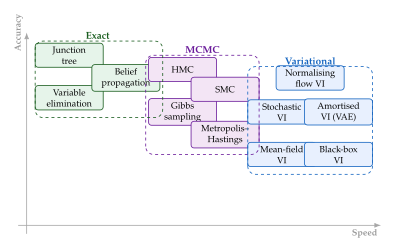
Figure 1 provides a bird's-eye view of inference methods, organised by their accuracy–speed trade-off.
The Core Idea: Inference as Optimisation
Key Idea.
Inference = Optimisation. Instead of computing analytically or sampling from it, variational inference posits a family of tractable distributions and solves the optimisation problem This converts an integration problem (hard) into a search problem (tractable with gradient-based methods). The quality of the approximation depends on the richness of the family .
Remark 1 (Why “Variational”?).
The name variational comes from the calculus of variations, the branch of mathematics concerned with optimising functionals, that is, functions of functions. Here we optimise the KL divergence, which is a functional of the distribution . When is a nonparametric family (e.g. all distributions that factorise in a certain way), the optimisation is genuinely variational: we take functional derivatives and set them to zero, exactly as in classical mechanics when deriving the Euler–Lagrange equations.
Road Map
The remainder of this chapter is organised as follows.
Section KL Divergence Revisited: KL Divergence Revisited. We examine the crucial asymmetry between forward and reverse KL, which determines why VI uses the reverse direction.
Section The Evidence Lower Bound: The Evidence Lower Bound. We derive the ELBO from multiple perspectives and explore its decompositions.
Section Mean-Field Variational Inference: Mean-Field VI. We introduce the fully factorised approximation and derive the optimal factors via functional optimisation.
Section Coordinate Ascent Variational Inference: Coordinate Ascent VI. We present the classical CAVI algorithm and apply it to Bayesian Gaussian mixture models.
File B continues with stochastic VI, amortised inference, and connections to VAEs (Chapter 15) and diffusion models (Chapter 19).
Insight.
The ELBO is the universal currency of deep generative models. Whether you are training a VAE (Chapter 15), a hierarchical VAE, or deriving the variational diffusion objective (Section ELBO for the Variational Diffusion Model), the ELBO appears as the central objective. Mastering its derivation and decompositions in this chapter will pay dividends across the rest of the book.
Why Posterior Inference Matters
Before diving into the technical machinery, let us emphasise why computing, or approximating, the posterior is so important. The posterior answers three distinct questions:
What do the latent variables look like? In a mixture model, the posterior tells us which cluster generated each observation. In a topic model, it tells us which topics are present in each document. In a VAE, it tells us the latent “code” that summarises each data point.
How uncertain are we? Bayesian posteriors quantify uncertainty. The posterior of a neural network's weights tells us not just the best-guess parameters but how confident we should be. This is crucial for safety-critical applications (medical diagnosis, autonomous driving) and for active learning (where we query the most uncertain inputs).
How do we learn model parameters? In the EM framework (Chapter 7), the E-step requires the posterior . In VAEs, the approximate posterior appears in the ELBO gradient. Posterior inference is not just a downstream task; it is integral to training.
Example 2 (The Posterior in Real Applications).
Medical imaging (VAE): A radiologist feeds a chest X-ray into a VAE. The approximate posterior compresses the image into a latent code . The spread of this posterior indicates how ambiguous the image is; a blurry or atypical scan produces a wider posterior, flagging it for human review.
Recommendation systems (matrix factorisation): The posterior over user and item latent factors quantifies our uncertainty about each user's preferences, allowing the system to recommend items that are both likely to be enjoyed and informative for reducing uncertainty.
Drug discovery (Bayesian optimisation): The posterior over a surrogate model's parameters drives the acquisition function that selects the next molecule to synthesise. Overconfident posteriors lead to premature exploitation; underconfident posteriors lead to wasteful exploration.
Remark 2 (The Inference–Learning Duality).
There is a deep duality between inference and learning:
Inference holds the model fixed and reasons about the latent variables: .
Learning holds the latent variables fixed (or marginalised) and adjusts the model: .
In the EM algorithm and in variational inference, these two problems are solved alternately: inference updates the latent variables, learning updates the parameters. The ELBO provides the objective for both.
KL Divergence Revisited
The KL divergence was introduced in Chapter 4 (Definition 3) and appeared naturally in the ELBO decomposition for GMMs (Proposition 3). In this section we examine a subtlety that is central to variational inference: the two directions of KL divergence behave very differently, and choosing the “wrong” direction would make VI impractical.
Recap: KL Divergence
Recall that for two continuous distributions with densities and on , the KL divergence from to is (DEF) By Gibbs' inequality (Theorem 1), with equality if and only if almost everywhere. Crucially, KL divergence is asymmetric: in general.
Forward vs. Reverse KL
Let denote the target distribution (in our setting, ) and the approximation. The two directions of KL divergence optimise very different objectives.
Definition 1 (Forward and Reverse KL).
The forward KL (or inclusive KL, moment-projection, M-projection) minimises (FWD KL)
The reverse KL (or exclusive KL, information-projection, I-projection) minimises (REV KL)
The terms “inclusive” and “exclusive” hint at the qualitative difference, which we now make precise.
Proposition 2 (Behaviour of Forward and Reverse KL).
Let be the target and the approximation.
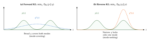
Forward KL is zero-avoiding (mode-covering): Wherever , the term in the forward KL blows up if . Hence the optimal must place mass everywhere does, even if this means spreading mass into low-density regions.
Reverse KL is zero-forcing (mode-seeking): Wherever , the term blows up if . Hence the optimal avoids placing mass where is small, even if this means ignoring entire modes of .
Proof.
For any with , the integrand in the forward KL contains as . Thus the minimum-KL solution must satisfy whenever : it covers all modes.
For any with , the reverse KL integrand contains as . Thus the minimum-KL solution must satisfy whenever : it avoids regions of zero target density and typically selects a single mode.
Visualising the Asymmetry
The following figure is perhaps the single most important illustration for understanding variational inference.
Why Reverse KL for Variational Inference
Given the mode-seeking behaviour of the reverse KL, one might ask: isn't the forward KL a better choice, since it covers all modes? The answer is no, for a pragmatic but decisive reason.
Proposition 3 (Computational Feasibility of the Two Directions).
Let be the intractable posterior and the approximation.
Forward KL requires , an expectation under the intractable posterior . We cannot compute this without already knowing the posterior.
Reverse KL requires , an expectation under the tractable approximation . We can compute (or estimate via Monte Carlo) this expectation because sampling from is easy.
Proof.
Expanding the forward KL: This requires sampling from or integrating over , which is precisely what we cannot do.
Expanding the reverse KL: All expectations are under , which we control. Moreover, we will show in Section The Evidence Lower Bound that minimising this quantity is equivalent to maximising the ELBO, which only requires evaluating the joint , not the intractable posterior.
Insight.
Forward KL needs the truth; reverse KL only needs your guess. The forward KL takes expectations under the unknown target , an apparent chicken-and-egg problem. The reverse KL takes expectations under the known approximation , which we designed to be easy to sample from. This computational asymmetry, not any preference for mode-seeking behaviour, is the primary reason variational inference uses the reverse KL.
Worked Example: Gaussian Approximation to a Mixture
To build intuition, let us compute both KL divergences explicitly for a toy problem.
Example 3 (Both KL Directions for a Mixture).
Let the target be a symmetric mixture of two unit-variance Gaussians: We approximate with a single Gaussian .
Forward KL. Since , and the entropy is independent of , minimising over amounts to maximising By symmetry of , the optimal mean is . Using (since and ), the optimal variance is . Hence , a very broad Gaussian straddling both modes, placing significant density in the valley at where .
Reverse KL. We minimise . The term is a log-sum-exp that cannot be computed in closed form, but we can optimise it numerically. Due to the mode-seeking property, gradient descent initialised near converges to , a tight Gaussian sitting on one mode and ignoring the other entirely.
Summary. The forward KL fit has the correct mean but wildly overestimates the variance. The reverse KL fit captures one mode precisely but misses the other.
Properties of KL Divergence
For completeness, we collect the key properties that will be used throughout.
Proposition 4 (Properties of KL Divergence).
Non-negativity (Gibbs' inequality): , with equality iff a.e.
Asymmetry: in general.
Not a metric: The triangle inequality does not hold.
Invariance under invertible transformations: If with a diffeomorphism, then .
Additivity for independent distributions: If and , then .
Chain rule: .
Proof of (d).
Let . Under the change of variables, , and similarly for . The Jacobian factors cancel in the ratio: This invariance is central to normalising flows, where the latent space is transformed through a chain of diffeomorphisms.
Remark 3 (Looking Ahead: Other Divergences in VI).
The restriction to reverse KL is a design choice, not a law of nature. Replacing it with other divergences yields different algorithms:
-divergence VI [4]: interpolates between forward and reverse KL using Rényi's -divergence.
Stein variational gradient descent (SVGD): uses the kernelised Stein discrepancy, combining the flexibility of particles with the speed of optimisation.
-divergence VI: gives tighter bounds on the marginal likelihood at the cost of higher variance gradients.
Each choice trades off bias, variance, and computational cost in different ways. We focus on the reverse KL because it leads directly to the ELBO.
The Evidence Lower Bound
The evidence lower bound (ELBO) is the central object of variational inference. It is simultaneously:
a lower bound on the log-evidence ,
the objective function that VI maximises,
a bridge between the intractable posterior and the tractable approximation.
We derive it from two complementary perspectives and then explore its multiple decomposition forms, each of which highlights a different aspect of the inference–learning trade-off.
Derivation Route 1: Jensen's Inequality
Theorem 1 (ELBO via Jensen's Inequality).
For any distribution over the latent variables, (Jensen) The quantity is called the evidence lower bound (ELBO).
Proof.
Start from the marginal likelihood and introduce : (Step1) The inequality in is Jensen's inequality applied to the concave function : for any positive random variable .
Remark 4 (Jensen's Gap).
The gap between and is sometimes called Jensen's gap. From our second derivation (below), we will see that this gap is exactly , the KL divergence from the approximation to the true posterior. Jensen's inequality is tight (gap ) if and only if the random variable inside the expectation is constant almost surely, which happens when .
Derivation Route 2: KL Decomposition
The second derivation is more revealing: it shows exactly where the gap comes from and why maximising the ELBO is equivalent to minimising the reverse KL divergence.
Theorem 2 (ELBO Gap Identity).
For any distribution , (GAP) Equivalently, (GAP ALT)
Proof.
Expand the KL divergence between and the true posterior : (Step1) In we used Bayes' theorem ; in the term exits the expectation because it does not depend on . Rearranging gives .
This is the same decomposition we encountered for GMMs in Proposition 3 (equation ), now stated in full generality. The identity has three immediate consequences:
Corollary 1 (Consequences of the ELBO Gap Identity).
Lower bound: Since , we have for all .
Maximising the ELBO minimising the KL: Since is constant with respect to ,
Tightness: The bound is tight () if and only if , i.e. a.e.
Key Idea.
The ELBO links three quantities. The log-evidence decomposes into the ELBO (what we can compute and optimise) plus the KL divergence (the approximation error we are trying to minimise). Since is fixed, pushing one up pushes the other down.
Three Decompositions of the ELBO
The ELBO can be written in several equivalent forms, each emphasising a different interpretation.
Proposition 5 (Three Faces of the ELBO).
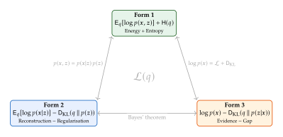
For any variational distribution , the ELBO admits the following equivalent decompositions: (Form1) where is the entropy of .
Proof.
Form 1: Expand the definition directly: Form 2: Factor the joint as : Form 3: This is a restatement of the ELBO gap identity .
Each form provides a different lens:
Energy + Entropy (Form 1): This is the classical variational free energy formulation from statistical physics. Maximising balances fitting the model (low energy = high ) against spreading out (high entropy ).
Reconstruction Regularisation (Form 2): This is the form most commonly used in VAEs (Section The Evidence Lower Bound). The first term rewards for concentrating on latent configurations that explain the data well; the KL term penalises for deviating from the prior, acting as a regulariser.
Evidence Gap (Form 3): This shows the ELBO as the log-evidence minus an approximation error. It is the most conceptually transparent form but the least computationally useful, since is unknown.
Worked Example: ELBO for a Gaussian Model
To solidify understanding, we compute the ELBO in closed form for a simple conjugate model.
Example 4 (ELBO for a Univariate Gaussian with Known Variance).
Suppose we observe with known variance and wish to infer the mean with a Gaussian prior .
True posterior (for reference). By conjugacy, the posterior is Gaussian: (TRUE Posterior) where .
Variational approximation. Let with free parameters . We compute the ELBO using Form 2:
Reconstruction term. using .
KL term. Using the formula for KL between univariate Gaussians (Proposition 1):
Optimal variational parameters. Setting and , we obtain The variational approximation recovers the exact posterior! This is expected: when the true posterior lies within the variational family (here, the family of all Gaussians), the ELBO is maximised at and the KL gap vanishes.
Remark 5 (Conjugacy and Tightness).
Example 4 is special: the true posterior is Gaussian, so a Gaussian variational family can capture it exactly. In most models of interest (VAEs, Bayesian neural networks, topic models), the true posterior is not in , and the ELBO is strictly below . The gap measures the price we pay for using a tractable approximation.
Tightness of the ELBO
Proposition 6 (ELBO Tightness Condition).
The ELBO is tight, , if and only if almost everywhere. Consequently:
If , then the optimal ELBO equals the log-evidence.
If , then the ELBO gap is , and the ELBO underestimates .
The ELBO as a Training Objective
In practice, the ELBO is used not only for inference (optimising ) but also for learning (optimising model parameters ). When the model has parameters (e.g. a neural network decoder), we maximise the ELBO jointly over and : (Joint) This is the principle behind the VAE objective (Section The Evidence Lower Bound): the encoder parameterises , the decoder parameterises , and both are optimised jointly via stochastic gradient ascent on the ELBO.
Example 5 (ELBO as a Lower Bound: Numerical Illustration).
Consider the conjugate model from Example 4 with observations , prior , and known variance .
The exact log-evidence can be computed: With , , and :
Now consider three variational approximations :
| Approximation | |||
| Optimal | |||
| Wide | |||
| Off-centre |
Connection to Statistical Physics
Remark 6 (The ELBO as Variational Free Energy).
In statistical physics, a system at inverse temperature has a Helmholtz free energy , where is the internal energy, is the temperature, and is the entropy. The Gibbs–Bogoliubov inequality states that for any trial distribution , with equality when is the Boltzmann distribution .
Setting and identifying , we see that . Thus maximising the ELBO is equivalent to minimising the variational free energy, the same principle that physicists have used since Gibbs (1902) and Bogoliubov (1958).
The ELBO and the Exponential Family
When the model belongs to the exponential family, the ELBO and its gradients take particularly clean forms. This is the setting where classical (non-stochastic) variational inference is most naturally derived.
Definition 2 (Exponential Family).
A distribution is in the exponential family with natural parameter if its density can be written as (Expfam) where is the vector of sufficient statistics, is the log-partition function, and is the base measure.
Proposition 7 (ELBO Gradient for Exponential-Family Models).
If is in the exponential family with natural parameters , then (Expfam GRAD) At the optimum, satisfies a fixed-point equation involving the expected sufficient statistics of the complete-data distribution under .
Remark 7 (Conjugate Models Are Especially Nice).
When the model is conditionally conjugate (each complete conditional belongs to the exponential family), the mean-field optimal factor from Theorem 3 is guaranteed to be in the same exponential family. This means:
The functional form of each is known a priori (Gaussian, Gamma, Dirichlet, etc.).
The update reduces to computing the natural parameters of , which are expectations of sufficient statistics.
No numerical optimisation is needed within each coordinate step, only moment computations.
This is why the BGMM example in Section Extended Example: CAVI for Bayesian Gaussian Mixture Models works so cleanly: the Dirichlet–Categorical and Gaussian–Gaussian conjugacies ensure all updates are in closed form.
The ELBO in Deep Generative Models
Remark 8 (Forward References: ELBO Across the Book).
The ELBO appears in many guises throughout this book:
GMMs (Section EM as Coordinate Ascent on the ELBO): the EM algorithm performs coordinate ascent on the ELBO with a discrete latent variable.
VAEs (Section The Evidence Lower Bound): the ELBO decomposes into reconstruction KL, optimised jointly over encoder and decoder via the reparameterisation trick.
Diffusion models (Section ELBO for the Variational Diffusion Model): the ELBO for a Markov chain of latent variables decomposes into a sum of local KL terms, one per diffusion step.
Hierarchical VAEs: the ELBO extends to multiple layers of latent variables, with the KL chain rule yielding a telescoping sum.
In every case, the ELBO serves the same dual purpose: it provides a tractable training objective and a measure of model quality.
Mean-Field Variational Inference
The ELBO gap identity (Theorem 2) tells us to maximise over a variational family . But which family? The choice of determines both the quality of the approximation and the difficulty of the optimisation. The simplest and historically most important choice is the mean-field family, in which the variational distribution factorises completely over the latent variables.
The Mean-Field Assumption
Definition 3 (Mean-Field Variational Family).
Let be a partition of the latent variables into groups (each may itself be a vector). The mean-field variational family is the set of distributions that factorise as (MF) Each factor is called a variational factor and is optimised independently. No parametric form is assumed for the factors; they are determined by the optimisation.
Historical Note.
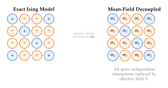
The mean-field idea originated in the physics of magnetism. Pierre-Ernest Weiss (1907) proposed that each spin in a ferromagnet experiences an effective “mean field” generated by the average of all other spins, rather than interacting with each one individually. This Curie–Weiss theory replaced a many-body problem with a single-body problem in an effective field, exactly the strategy of mean-field VI. The extension to general probabilistic models was formalised by Jordan et al. (1999) [2], who recognised that the same decoupling principle applies to any graphical model.
The mean-field assumption is drastic: by forcing , we ignore all correlations between the groups . If the true posterior has strong dependencies between latent variables, as it often does, this introduces bias. But the payoff is computational: the optimal factors have a remarkably simple form.
Optimal Mean-Field Factors
Theorem 3 (Optimal Mean-Field Update).
Under the mean-field assumption , the ELBO is maximised with respect to a single factor , holding all others fixed, when (Optimal) where denotes the expectation with respect to all variational factors except : Equivalently, (Optimal EXP)
Proof.
We isolate the dependence of the ELBO on . Write and expand: (Proof Expand) The last line (entropies of other factors) is constant with respect to . Define . The terms involving are: (Proof KL) Define . Then where is the normalisation constant of . Since , the maximum is attained at , i.e. .
Remark 9 (Functional Optimisation).
Theorem 3 is a result from the calculus of variations: we optimise the functional with respect to the function , with no parametric assumption on . The optimal is determined entirely by the model's joint distribution and the current values of the other factors. In practice, if the model is in the exponential family, the optimal belongs to a recognisable parametric family (Gaussian, Gamma, Dirichlet, etc.), and the update reduces to computing its natural parameters.
Example: Mean-Field for the Ising Model
The Ising model is the prototypical example from statistical physics.
Example 6 (Mean-Field Ising Model).
Consider a lattice of binary spins with pairwise interactions: where is the set of edges (e.g. nearest neighbours on a grid), are coupling strengths, are external fields, and is the (intractable) partition function.
Mean-field approximation. Assume , where each is a Bernoulli distribution parameterised by .
By Theorem 3: where are the neighbours of spin and . Normalising: Each spin's magnetisation is determined by the average magnetisation of its neighbours, the “mean field” that gives the method its name.
Example: Mean-Field for a Bivariate Gaussian
Before tackling a full model, let us see mean-field VI in action on the simplest possible example: a two-dimensional Gaussian.
Example 7 (Mean-Field for a Correlated Bivariate Gaussian).
Let with . We apply the mean-field factorisation .
Optimal . By Theorem 3: Let . Completing the square: .
Optimal . By symmetry: .
Fixed point. The coupled system and has the unique solution (since ). Hence:
What is lost? The marginal means are correct (), but the marginal variances are instead of the true value . The mean-field approximation underestimates the marginal variances, and of course sets the covariance to zero. The KL gap is As , this gap diverges; the mean-field approximation becomes arbitrarily poor for strongly correlated variables.
This simple example encapsulates the core trade-off of mean-field VI: tractability (independent factors) versus fidelity (capturing correlations).
Example: Mean-Field for Bayesian Linear Regression
We now apply mean-field VI to a workhorse statistical model.
Example 8 (Mean-Field Bayesian Linear Regression).
Consider the Bayesian linear regression model: (Prior TAU) where is the noise precision, is the weight vector, and are training pairs.
Mean-field factorisation. We posit , a complete factorisation between weights and precision.
Optimal factor for . By Theorem 3: where . This is a quadratic form in , so with (QW)
Optimal factor for . Similarly: This is the log-density of a Gamma distribution: with (QTAU) The expectation in uses .
Key observation. The optimal depends on (from ), and the optimal depends on moments of . Neither can be computed independently: we must iterate, updating one factor while holding the other fixed. This is the coordinate ascent algorithm of Section Coordinate Ascent Variational Inference.
Mean-Field vs. Exact Posterior
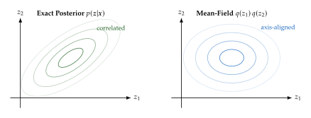
The mean-field approximation decouples the latent variables, which means it cannot represent posterior correlations. The following figure illustrates this concretely.
Caution.
Mean field ignores correlations. The mean-field approximation sets all posterior covariances between different groups to zero: for . This can cause:
Underestimation of posterior variance in individual variables (the marginal may be too narrow because it cannot “borrow” uncertainty from correlated variables).
Poor uncertainty quantification in downstream tasks that depend on joint distributions (e.g. predictive intervals).
Overconfident predictions in Bayesian models where parameter correlations are important (e.g. multicollinear regression).
When correlations are critical, consider structured VI (e.g. block mean-field, Gaussian with full covariance, or normalising-flow families) at the cost of harder optimisation.
Structured Variational Families
Proposition 8 (Mean-Field Is Dominated by Structured Approximations).
Let , where is a structured family that preserves some dependencies. Then A richer variational family always yields a tighter (or equal) ELBO, at the cost of harder optimisation.
Proof.
Since , the maximum over the larger set is at least as large. The upper bound follows from the ELBO gap identity.
Remark 10 (Beyond Mean Field).
Common structured families include:
Block mean-field: Group related variables and allow correlations within blocks:
Gaussian with full covariance: with a full (or low-rank + diagonal) covariance matrix.
Normalising-flow families: Transform a simple base distribution through a sequence of invertible maps, allowing to capture complex dependencies.
Amortised inference: Use a neural network to map each observation to its own approximate posterior, the approach of VAEs (Definition 4).
Each choice moves up the accuracy–cost trade-off curve of Figure 1.
Coordinate Ascent Variational Inference
The optimal mean-field updates of Theorem 3 give us the best factor when all other factors are held fixed. But each update depends on the moments of the other factors, creating a system of coupled equations. The natural solution is to iterate: update each factor in turn, cycling through all groups. This is the coordinate ascent variational inference (CAVI) algorithm.
The CAVI Algorithm
Algorithm 1 (Coordinate Ascent Variational Inference (CAVI)).
Input: Model , data , partition .
Output: Variational factors .
Initialise: Set each factor to a reasonable initialisation (e.g. random, prior, or moment-matched).
for until convergence:
for : enumerate[(a)]
Compute the expected log-joint under all factors except :
Normalise to obtain a valid density.
Extract the sufficient statistics / moments of needed by other updates. enumerate
Compute to monitor convergence.
if , stop.
Monotonic Convergence
Theorem 4 (CAVI Monotonically Increases the ELBO).
Each CAVI update (updating a single factor while holding others fixed) increases , or leaves it unchanged if is already optimal. Consequently, the sequence is non-decreasing.
Proof.
From the proof of Theorem 3, the ELBO restricted to (with all other factors fixed) is where . The CAVI update sets , achieving and thus maximising . Since , the full ELBO cannot decrease.
Since the ELBO is bounded above by , the monotone bounded sequence converges.
Remark 11 (Local Optima).
CAVI is guaranteed to converge to a local maximum (or saddle point) of the ELBO, not necessarily the global maximum. The ELBO landscape for mean-field VI is generally non-convex, even when the model is in the exponential family. In practice:
Multiple random initialisations are used, and the run with the highest final ELBO is selected.
The initialisation can significantly affect both the speed of convergence and the quality of the solution.
For mixture models, the symmetry of the model means that permuting cluster labels gives equivalent solutions (the “label-switching” problem).
Extended Example: CAVI for Bayesian Gaussian Mixture Models
We now develop a complete CAVI algorithm for the Bayesian Gaussian mixture model (BGMM), the canonical example in variational inference. This extends the EM algorithm of Chapter 7 by placing priors on all parameters and performing fully Bayesian inference.
Example 9 (Bayesian Gaussian Mixture Model - Full Specification).
Generative model. For components in with observations: (PI) where we use isotropic covariances (known) for simplicity. The latent variables are .
Joint log-density. (Joint)
Variational factorisation. We use the mean-field factorisation: (MF)
We now derive each optimal factor using Theorem 3.
Update for : Cluster Assignments
The terms in that involve are and . By Theorem 3: (Z Update) Define the “responsibility” parameters: (RHO) normalised so that . These are the variational analogue of the EM responsibilities (Section The EM Algorithm for GMMs).
The expectations needed are:
: the digamma function, computed from the Dirichlet factor .
, where are the mean and covariance of .
Update for : Cluster Means
The terms involving are and the likelihood terms for all assigned to cluster : (MU LOG) Completing the square in , this is Gaussian: (Q MU) with (MU Params) where is the effective number of points assigned to cluster . This is a precision-weighted average of the prior mean and the data centroid .
Update for : Mixing Weights
The terms involving are (the Dirichlet prior) and : (PI LOG) This is the log-density of a Dirichlet distribution: (Q PI) The expected log-mixing weights needed by the -update are: (Elogpi) where is the digamma function .
Summary of CAVI Updates
Algorithm 2 (CAVI for Bayesian GMM).
Computing the ELBO for Monitoring
To monitor convergence, we must evaluate the ELBO at each iteration. Using the mean-field factorisation :
(ELBO FULL)
Each term involves expectations of log-densities under their respective variational factors, all of which are available in closed form for exponential-family models:
Dirichlet terms: involves the difference of two Dirichlet log-normalisation constants plus digamma expectations.
Gaussian mean terms: , computable via the closed-form KL between Gaussians (Proposition 2).
Data terms: ; the reconstruction term uses ; the entropy of is .
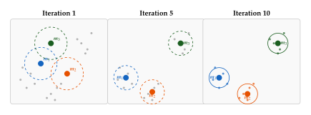
CAVI Iterations: A Visual Example
Comparison with EM
CAVI for the Bayesian GMM bears a striking resemblance to EM for the frequentist GMM (Chapter 7). The following table makes the correspondence explicit.
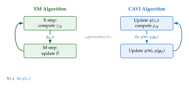
Proposition 9 (EM as a Special Case of CAVI).
If the variational family for the parameters is restricted to point masses , then CAVI reduces to the EM algorithm:
The update becomes the E-step (computing responsibilities under the current ).
The “update” becomes the M-step (finding the that maximises the expected complete-data log-likelihood).
Proof.
With , the expected log-joint evaluated at gives the same responsibilities as the E-step. Maximising the ELBO over with fixed is equivalent to maximising , which is the M-step objective .
Practical Considerations
Remark 12 (Initialisation Strategies).
Good initialisation is critical for CAVI:
-means initialisation: Run -means on the data and use the cluster assignments to initialise . This is the most common strategy.
Random initialisation: Draw from a Dirichlet distribution and normalise. Repeat with multiple random seeds.
Prior initialisation: Set variational parameters to the prior hyperparameters. This is conservative but can be slow to converge.
Spectral initialisation: Use the leading eigenvectors of the data matrix for initial cluster structure.
Remark 13 (Convergence Diagnostics).
In practice, CAVI convergence is monitored by tracking the ELBO across iterations. Additional diagnostics include:
Checking that the ELBO is monotonically non-decreasing (any decrease indicates a bug).
Monitoring the change in variational parameters between iterations.
For mixture models, tracking the effective number of clusters .
Typical convergence occurs in – iterations for well-initialised models, though this depends on the model complexity and data size.
Remark 14 (CAVI as Message Passing).
The CAVI updates have an elegant interpretation as message passing on the graphical model. Each factor sends “messages” (its sufficient statistics) to the factors it interacts with through the joint distribution. This perspective, formalised as variational message passing (VMP) [5], allows automatic derivation of CAVI updates for any conjugate exponential-family model. Software packages such as Infer.NET and Edward implement this paradigm.
CAVI and Natural Gradients
There is an elegant connection between the CAVI coordinate updates and the natural gradient of information geometry.
Proposition 10 (CAVI Performs Natural Gradient Ascent).
When each factor belongs to an exponential family with natural parameters , the CAVI update is equivalent to a natural gradient step with unit step size: (Natgrad) where is the Fisher information matrix of . In the natural parameterisation, simplifies, and the update becomes a direct replacement of natural parameters.
This connection is important because it explains why CAVI converges rapidly in practice: natural gradients account for the curvature of the distribution space and take optimally large steps. It also paves the way for stochastic natural-gradient methods, where we replace the full-data sufficient statistics with mini-batch estimates, the basis of stochastic variational inference (SVI), covered in File B.
Predictive Distribution
After convergence, the variational approximation can be used for prediction. For the Bayesian GMM, the predictive density for a new observation is:
(Predictive)
Since both the likelihood and are Gaussian, the inner integral is available in closed form:
(Predictive Closed)
The predictive distribution is therefore itself a Gaussian mixture with . Notice that the predictive covariance is larger than the noise covariance : the additional term captures our epistemic uncertainty about the cluster mean. As , and the predictive distribution converges to the plug-in estimate, and the Bayesian and frequentist answers agree asymptotically.
Remark 15 (Model Comparison via the ELBO).
Since the ELBO lower-bounds , it can serve as a proxy for Bayesian model comparison. Given two models and , we prefer the one with the higher optimised ELBO: This is an automatic, principled alternative to BIC/AIC that naturally penalises model complexity through the KL regularisation term. For the BGMM, this approach can determine the number of clusters without cross-validation: simply run CAVI for several values of and select the with the highest ELBO.
Limitations of CAVI
Caution.
When CAVI falls short. Despite its elegance, classical CAVI has significant limitations:
Requires conjugacy: The optimal factor is only tractable when the model is conjugate exponential family. Non-conjugate models require approximations within each update.
Does not scale to large datasets: Each update sweeps over all data points. For , this is prohibitively expensive.
Mean-field bias: The factorised approximation ignores posterior correlations, which may be severe.
Local optima: The non-convex ELBO landscape means results depend on initialisation.
No amortisation: Each new data point requires re-running the full optimisation, and there is no way to “generalise” the inference to unseen inputs.
These limitations motivate the development of stochastic variational inference (which scales to large data), black-box VI (which handles non-conjugate models), and amortised VI (which generalises across data points), all of which are covered in File B of this chapter. The amortised approach leads directly to the VAE (Chapter 15).
Exercises
Exercise 1 (ELBO Derivation).
Derive the ELBO via Jensen's inequality, starting from .
Derive the ELBO via the KL decomposition, starting from .
Show that the two derivations yield the same expression.
Under what condition is the bound tight?
Exercise 2 (Forward vs. Reverse KL).
Let and .
Find the optimal minimising analytically.
Argue that the optimal minimising concentrates on one mode. Use gradient descent to find the solution numerically.
Plot both approximations and the target. Which captures the “shape” of better? Which captures a “mode” better?
For what kinds of downstream tasks would you prefer the forward KL approximation? The reverse?
Exercise 3 (ELBO for a Poisson Model).
Consider the model and for .
Write the joint log-density .
Let . Compute the ELBO in closed form.
Find the optimal by setting gradients to zero. Verify that these recover the exact posterior parameters (since the model is conjugate).
Compute the ELBO at the optimum and verify that it equals .
Exercise 4 (Mean-Field for a Bivariate Gaussian).
Let with .
Apply the mean-field factorisation .
Using Theorem 3, derive the optimal and . Show that they are Gaussian with the correct marginal means and variances.
Compute as a function of . What happens as ?
Plot the contours of , , and their difference for .
Exercise 5 (CAVI for Bayesian Linear Regression).
Implement CAVI for the Bayesian linear regression model of Example 8.
Generate synthetic data from with , , .
Initialise and and run CAVI for 50 iterations. Plot the ELBO vs. iteration.
Compare the variational posterior means with the true values and with the MLE .
Plot the marginal posteriors and and compare with the exact Bayesian posterior (available in closed form for this conjugate model).
Vary and describe how the posterior concentrates as grows.
Exercise 6 (CAVI for Bayesian GMM).
Implement the CAVI algorithm for the Bayesian GMM (Algorithm 2).
Generate 300 data points from a mixture of 3 Gaussians in .
Run CAVI with (intentionally over-specified). Plot the ELBO vs. iteration and the cluster assignments at convergence.
Observe that some clusters become “empty” (). How does the Dirichlet prior encourage this automatic pruning?
Compare the converged cluster means and effective counts with the EM solution.
Repeat with different initialisations. How sensitive is the solution?
Exercise 7 (ELBO Monotonicity).
Prove that each coordinate update in CAVI increases (or maintains) the ELBO.
Show that the ELBO is bounded above by .
Conclude that CAVI converges.
Give an example where CAVI converges to a local (non-global) maximum.
Exercise 8 (Stein Variational Gradient Descent).
SVGD [6] represents the variational distribution as a set of particles updated by where is a positive-definite kernel.
Explain why the first term in drives particles toward high-density regions of the posterior.
Explain why the second term (the “repulsive” term) prevents particles from collapsing to a single point.
In the limit , show that SVGD reduces to gradient ascent on (i.e. MAP inference).
Compare SVGD with mean-field VI: which can represent multimodal posteriors?
Exercise 9 (Importance-Weighted ELBO).
The standard ELBO uses a single-sample estimate. The importance-weighted ELBO (IWAE bound) [7] draws samples from :
Show that (the standard ELBO).
Use Jensen's inequality to show that for all . (Hint: the of an average is at most the average of s.)
Show that .
Discuss the trade-off: more samples give a tighter bound but increase computational cost. When might be worthwhile?
Remark 16 (Summary and Looking Ahead).
In this chapter we have developed the foundations of variational inference:
Section KL Divergence Revisited: The asymmetry of KL divergence (forward KL is mode-covering, reverse KL is mode-seeking) and the computational reason that VI uses the reverse direction.
Section The Evidence Lower Bound: The ELBO, derived via Jensen's inequality and the KL decomposition, with three equivalent forms (energy entropy, reconstruction regularisation, evidence gap).
Section Mean-Field Variational Inference: The mean-field assumption, which yields optimal factors via functional optimisation at the cost of ignoring posterior correlations.
Section Coordinate Ascent Variational Inference: The CAVI algorithm, which iterates mean-field updates to convergence, with a complete worked example for Bayesian GMMs.
Classical CAVI is limited to conjugate exponential-family models and does not scale to large datasets or deep generative models. File B addresses these limitations through stochastic variational inference (mini-batch updates), black-box variational inference (score function and reparameterisation gradients), and amortised inference (neural network encoders). The amortised approach connects directly to the VAE (Chapter 15), where the encoder plays the role of the variational distribution and the ELBO is maximised end-to-end with the reparameterisation trick.
Exponential Families and Conjugacy
The coordinate ascent updates derived in the previous section, while general in principle, become especially clean and computationally attractive when the model belongs to the exponential family. This is no accident: exponential families possess a rich algebraic structure that interacts beautifully with the KL divergence and the ELBO. In this section we formalise this structure and show why exponential families occupy a privileged position in variational inference.
The Exponential Family
Definition 4 (Exponential Family).
A parametric family of distributions is an exponential family if every member can be written in the form (Recap) where:
is the natural parameter (also called the canonical parameter).
is the vector of sufficient statistics.
is the base measure, independent of .
is the log-partition function (also called the cumulant function), which ensures normalisation.
The set is the natural parameter space.
The exponential family encompasses nearly every distribution encountered in introductory statistics: the Gaussian, Bernoulli, Poisson, exponential, gamma, beta, Dirichlet, multinomial, Wishart, and von Mises–Fisher distributions are all members. Notable exceptions include the uniform distribution on (whose support depends on the parameter), the Cauchy distribution (no sufficient statistic of fixed dimension), and mixture distributions (sums of exponentials are not exponentials).
The representation may look abstract, but its power lies in the properties of the log-partition function . The function acts as a “generating function” for the moments of : each derivative of produces a higher moment.
Theorem 5 (Properties of the Log-Partition Function).
Let be a member of an exponential family with log-partition function . Then:
is convex in .
The mean of the sufficient statistics is given by the gradient: (MEAN)
The covariance of the sufficient statistics is given by the Hessian: (COV)
Proof.
Part 1. Write . This is the logarithm of a sum (integral) of convex functions of (exponentials are convex), hence convex (log-sum-exp is convex; see the appendix on convex analysis).
Part 2. Differentiate under the integral sign:
Part 3. Differentiating once more: Since a covariance matrix is positive semi-definite, the Hessian of is positive semi-definite, confirming convexity.
Example 10 (The Gaussian as an Exponential Family).
A univariate Gaussian can be rewritten: Identifying the components:
Natural parameters: .
Sufficient statistics: .
Base measure: .
Log-partition function: .
One can verify that and , as promised by Theorem 5.
Example 11 (The Bernoulli as an Exponential Family).
The Bernoulli distribution for can be rewritten: Identifying the components:
Natural parameter: (the log-odds or logit).
Sufficient statistic: .
Base measure: .
Log-partition function: .
We can verify: , where is the logistic sigmoid, and .
Remark 17 (Mean Parameters and Natural Parameters).
The mapping sends natural parameters to mean parameters . Because is convex (Theorem 5), this mapping is monotone and, for minimal exponential families (where the sufficient statistics are not linearly dependent), it is a bijection. The inverse mapping is available via the convex conjugate .
This duality between natural and mean parameters is the foundation of the information geometry of exponential families, and it plays a key role in the natural gradient methods discussed in Stochastic Variational Inference.
The KL divergence between two members of the same exponential family has a particularly elegant form: (KL) This is the Bregman divergence generated by , a connection that provides geometric insight into variational inference as projection onto the variational family with respect to this divergence.
Conjugate Priors
When building Bayesian models, a natural question is: can we choose a prior so that the posterior has the same functional form as the prior? If so, the posterior update becomes a simple parameter update rather than a change of distributional family.
Definition 5 (Conjugate Prior).
Let be a likelihood from an exponential family. A prior is conjugate to this likelihood if, for any observation , the posterior belongs to the same family as the prior.
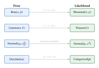
When the likelihood belongs to an exponential family with natural parameter and sufficient statistics , a conjugate prior can always be constructed: (FORM) where and are hyperparameters, and is the normalising constant. After observing data , the posterior is (Posterior) which is the same family with updated hyperparameters and . The posterior simply “adds” the observed sufficient statistics to the prior pseudo-observations.
CAVI in Exponential Family Models
We now connect exponential families to the coordinate ascent variational inference (CAVI) algorithm developed in the previous section. The payoff is remarkable: for models in which every complete conditional belongs to an exponential family, the optimal mean-field factors have closed-form natural parameter updates.
Theorem 6 (Optimal Mean-Field Factor for Exponential Family Complete Conditionals).
Suppose the complete conditional of latent variable given all others is an exponential family: (Conditional) Then the optimal mean-field variational factor is in the same exponential family: (Optimal) That is, the optimal variational natural parameter is the expected natural parameter of the complete conditional, where the expectation is taken under the current variational distribution over all other variables: (Natparam)
Proof.
Recall from the CAVI derivation that the optimal satisfies Since only the terms in that involve matter, and the complete conditional absorbs all such terms: The term does not depend on and is absorbed into the constant. Exponentiating gives , which is an exponential family distribution with natural parameter .
Example 12 (Conjugate Updates: Normal–Normal Model).
Consider a simple model with known variance : a Gaussian prior on the mean and Gaussian observations: (Model) The complete conditional of given the data is where (Posterior) In this simple case the posterior is exact (no approximation needed), but the structure illustrates the general pattern: the natural parameter of the posterior is the sum of the prior natural parameter and the data natural parameter. In the Gaussian case, the natural parameter is (the precision-weighted mean), and we see that the posterior natural parameter is , the prior pseudo-data plus the actual data, exactly as predicts.
Insight.
Why exponential families are special for VI. Exponential families enjoy three properties that make variational inference tractable and elegant:
Closed-form CAVI updates. The optimal mean-field factor belongs to the same family as the complete conditional, and its natural parameter is simply an expectation (Theorem 6). No optimisation subroutine is needed.
Moment–parameter duality. The gradient of maps natural parameters to mean parameters (Theorem 5), providing a bijection between two coordinate systems, each useful for different computations.
Finite-dimensional sufficient statistics. The entire dataset is summarised by , which is crucial for the scalable methods we develop next.
When any of these properties fails (for example, when the model has non-conjugate factors), the elegant closed-form updates break down, motivating the more general techniques in sec:vi:bbvi,sec:vi:reparam.
The Variational EM Algorithm
In The EM Algorithm for GMMs we introduced the Expectation–Maximisation (EM) algorithm for fitting models with latent variables. Recall the two steps:
E-step: compute the posterior over latent variables, .
M-step: maximise the expected complete-data log-likelihood with respect to the model parameters .
For GMMs, the E-step is tractable: the posterior over the cluster assignments factorises and each factor is a categorical distribution (the “responsibilities”). But for more complex models (topic models, deep latent variable models, models with continuous high-dimensional latent spaces) the exact posterior is intractable. What do we do?
The answer is the Variational EM algorithm: replace the exact E-step with a variational E-step that finds an approximate posterior within a tractable family .
To understand why the exact E-step becomes intractable, consider a topic model with topics and a document of words. The posterior over topic assignments requires marginalising over all possible configurations, an exponential sum that no closed-form trick can simplify. In a deep latent variable model, the decoder is a neural network, and the posterior involves inverting this nonlinear mapping, and there is no hope of a closed form. Variational EM sidesteps these difficulties by approximating the posterior rather than computing it exactly.
Historical Note.
The variational EM framework was developed and popularised in the mid-1990s and early 2000s, with foundational contributions by Jordan et al. [2] and Winn and Bishop [5], who developed the VIBES (Variational Inference for Bayesian Networks) software that automated variational updates for conjugate exponential family models. The application to LDA by Blei et al. [8] demonstrated that variational methods could scale to real-world text corpora, sparking widespread adoption in machine learning.
From EM to Variational EM
Recall the ELBO decomposition (from the previous sections): (Decomp) In standard EM, the E-step sets , making the KL term zero and the ELBO equal to the log-evidence. In variational EM, we cannot set to the exact posterior; instead, we maximise the ELBO over a restricted family :
Definition 6 (Variational E-step and M-step).
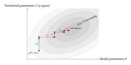
VE-step (variational E-step): holding fixed at , find (Vestep) This is equivalent to minimising over .
VM-step (variational M-step): holding fixed at , update the model parameters: (Vmstep) Since the entropy does not depend on , this reduces to .
Algorithm 3 (Variational EM Algorithm).
- Initialise model parameters and variational parameters
- for until convergence
- VE-step: optimise variational parameters Approximate posterior
- VM-step: optimise model parameters Fit generative model
- Evaluate and check for convergence
Theorem 7 (Monotonic Convergence of Variational EM).
Each iteration of Variational EM increases the ELBO: (Monotone) Since the ELBO is bounded above by (which itself is bounded for well-defined models), the sequence converges.
Proof.
The first inequality follows because the VE-step maximises over while holding fixed, so the new achieves an ELBO at least as large as the old . The second inequality follows because the VM-step maximises over while holding fixed. Each step is a (block) coordinate ascent on the ELBO, and since the ELBO is bounded above, the sequence converges.
Remark 18 (Connection to Standard EM).
When the variational family is unrestricted (i.e., all valid distributions), the VE-step recovers the exact posterior , and Variational EM reduces to standard EM\@. The difference is entirely in the restriction of : mean-field assumptions, parametric families, or amortised inference networks.
The restriction has two consequences. First, the ELBO at convergence will generally be lower than the true log-likelihood; the gap equals the KL divergence between the best approximation in and the true posterior. Second, the VM-step may converge to a different than standard EM would, because the objective being maximised (the ELBO with an approximate ) differs from the exact expected complete-data log-likelihood. Despite this, Variational EM often finds good solutions in practice, and it is the only option when the exact E-step is intractable.
Example: Variational EM for Latent Dirichlet Allocation
Latent Dirichlet Allocation (LDA) is the canonical application of Variational EM [8]. It is a topic model that discovers latent “topics” (distributions over words) from a corpus of documents.
The generative model. For a corpus of documents, each with words, and latent topics:
For each topic : draw a word distribution , where (the -simplex over a vocabulary of words).
For each document : enumerate
Draw topic proportions .
For each word position : enumerate
Draw a topic assignment .
Draw a word . enumerate enumerate
The posterior is intractable because the Dirichlet–categorical conjugacy is broken by the coupling through the topic assignments .
The mean-field approximation. The standard variational approximation uses a fully factorised family: (MF) where , , and .
Example 13 (Variational EM for LDA).
VE-step. Applying CAVI with exponential family structure (Theorem 6), the updates cycle through the local variational parameters: (PHI) where uses the digamma function .
VM-step. The global topic–word parameters are updated as: (Lambda) This aggregates the expected topic assignment across all documents: counts how many times word is (softly) assigned to topic , plus the prior pseudo-count .
The computational cost of each VE-step is , where is the average document length: we must update for each of the word positions and topics. For a corpus of documents with average length and topics, a single VE-step touches variational parameters.
Moreover, the VE-step must be iterated to convergence (cycling through the and updates multiple times) before performing a single VM-step. This makes each iteration of Variational EM extremely expensive for large corpora.
The VM-step aggregates information from all documents to update the global topic parameters. This full-data sweep is the computational bottleneck that motivates the stochastic methods of the next section.
Remark 19 (Sparsity in LDA).
Stochastic Variational Inference
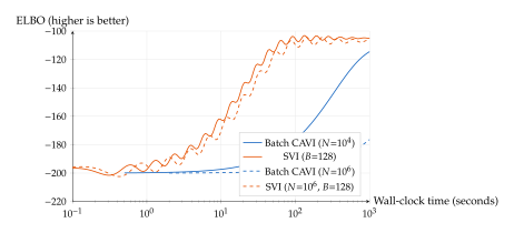
Coordinate ascent variational inference (CAVI) and Variational EM both require a full pass over the dataset in every iteration. For the LDA example, each VE-step touches every word in every document. When the corpus grows from thousands to millions of documents, this becomes a crippling bottleneck: the cost of a single iteration scales linearly in the dataset size , and many iterations are needed for convergence.
The insight of Stochastic Variational Inference (SVI) [20] is both natural and powerful: subsample the data and use noisy but unbiased gradient estimates to update the global variational parameters. This brings the per-iteration cost down from to (independent of dataset size), at the price of noisier updates that nonetheless converge to the same optimum.
Local and Global Latent Variables
The key structural assumption in SVI is a distinction between two types of latent variables.
Definition 7 (Local and Global Variables).
In a latent variable model with data :
Local (latent) variables are associated with a single data point . There are sets of local variables, one per observation.
Global (latent) variables are shared across all data points. They govern the overall structure of the model.
The joint model factorises as: (Model)
In LDA, the topic–word distributions are global variables (shared across all documents), while the topic proportions and topic assignments are local to document . In a Gaussian mixture model, the component parameters are global, and the cluster assignments are local.
The mean-field variational distribution mirrors this decomposition: (MF) where are the global variational parameters and are the local variational parameters for data point .
The SVI Algorithm
The ELBO for the model decomposes as: (ELBO) The sum over data points is the bottleneck. The SVI strategy proceeds in three steps:
Subsample a minibatch of size .
Local step: for each , optimise to convergence (using the current global parameters ). This is typically cheap, often one CAVI update per local variable.
Global step: form the stochastic natural gradient of the ELBO with respect to and take a step.
The stochastic gradient is constructed by scaling the minibatch contribution: (GRAD) The factor rescales the minibatch contribution to be an unbiased estimate of the full-data sum.
For conjugate exponential family models, the global update takes a particularly elegant form. After computing the locally optimal for each , the intermediate global natural parameter is (Intermediate) where encodes the prior's contribution and are the expected sufficient statistics from data point under the optimised local distribution. The global update is then a convex combination (weighted average) of the old parameters and this intermediate estimate: (Update) where is the step size (learning rate) at iteration .
Algorithm 4 (Stochastic Variational Inference).
- Initialise global variational parameters
- Set step size schedule with ,
- for
- Sample a minibatch uniformly,
- for each Local step
- Optimise local parameters:
- Compute intermediate global parameter: Global step
- Update:
Why Natural Gradients?
A crucial but subtle point in the SVI algorithm is that the global update uses the natural gradient rather than the ordinary (Euclidean) gradient. To understand why, consider the geometry of the variational parameter space.
The ordinary gradient gives the steepest ascent direction in Euclidean space; it assumes that a unit step in any direction of produces an equally significant change. But for probability distributions, this is misleading: a change in the mean of a Gaussian has a very different effect from the same change in the log-variance.
The natural gradient corrects for this by measuring distances in the space of distributions rather than parameters. It is defined as: (Natgrad) where is the Fisher information matrix.
For exponential families, a remarkable simplification occurs: when the variational parameters are the natural parameters , the Fisher information matrix is , and the natural gradient update in natural parameter space takes the simple form of the convex combination . This is why SVI works in natural parameter space, where the natural gradient is “built in” to the update rule.
Remark 20 (Natural vs. Euclidean Gradients).
In practice, natural gradient updates converge significantly faster than ordinary gradient updates for VI, because they account for the curvature of the KL divergence landscape. Ordinary gradient descent can take many small steps in high-curvature directions while overshooting in low-curvature directions; the natural gradient normalises step sizes appropriately across all directions. We will explore natural gradients in more depth in the next chapter section.
Convergence Guarantees
The step size schedule must satisfy the classical Robbins–Monro conditions [9]: (Robbins) The first condition ensures that the step sizes are large enough to reach any point in parameter space (no matter how far the initialisation is from the optimum). The second condition ensures that the noise in the stochastic gradient is eventually averaged out. The schedule satisfies both conditions when .
Theorem 8 (Convergence of SVI).
Under the following conditions:
The model–variational family pair yields an ELBO (with local variables optimised out) that has a unique global optimum .
The stochastic natural gradient is an unbiased estimate of the true natural gradient with bounded variance.
Then the SVI iterates converge to the global optimum: almost surely as .
More generally, when the ELBO has multiple local optima, SVI converges to a local optimum of the ELBO.
Proof sketch.
The update has the form of a stochastic approximation scheme: . This is a Robbins–Monro recursion with the expected update pointing towards the optimum of the ELBO (since at convergence for the single-optimum case). The conditions on ensure that the iterates eventually overcome the noise (first condition) without accumulating too much variance (second condition). The result then follows from the classical Robbins–Monro theorem.
Example: SVI for Online Topic Modelling
Example 14 (SVI for LDA with Streaming Documents).
Consider applying SVI to the LDA model from Example 13. The global variables are the topic–word distributions with variational parameters (each ). The local variables are the per-document topic proportions and word-level topic assignments , with variational parameters and .
In each SVI iteration:
Sample a minibatch of documents.
Local step: for each , iterate the CAVI updates – to convergence, obtaining and .
Global step: compute the intermediate topic parameters: and update .
Because only the documents in are processed, a single SVI iteration on a corpus of documents costs the same as on a corpus of documents (given the same minibatch size ). This makes it possible to learn topic models from web-scale text corpora in a streaming fashion: new documents can be incorporated as they arrive, without revisiting old ones.
Key Idea.
Subsample Data, Scale Gradients. The core principle of SVI is simple: replace the expensive full-data gradient with a cheap, noisy, but unbiased estimate computed from a small minibatch. The stochastic approximation theory of Robbins and Monro [9] guarantees convergence, provided the step sizes decay at the right rate. This is the same principle that makes stochastic gradient descent (SGD) work for training neural networks, applied here to variational inference.
The limitation of SVI is that it still requires model-specific derivations: the practitioner must work out the conjugate structure, derive the natural gradient, and implement the local and global updates by hand. The next two sections remove this limitation.
Black-Box Variational Inference
Stochastic variational inference (Stochastic Variational Inference) brought scalability to VI, but it required the practitioner to derive model-specific update equations, exploiting conjugate exponential family structure to obtain closed-form natural gradients. What if the model is not conjugate? What if the likelihood involves a neural network, or the prior is non-standard? In such cases, the elegant closed-form updates of SVI simply do not exist.
Black-Box Variational Inference (BBVI) [21] attacks this problem head-on: it provides a gradient estimator for the ELBO that works for any model and any variational family, requiring only the ability to
sample from the variational distribution , and
evaluate and at the sampled points.
No conjugacy, no exponential family structure, no model-specific derivations. The price? Variance, which we must work hard to control.
The Score Function Estimator
The foundation of BBVI is the score function estimator, also known as the REINFORCE trick or the log-derivative trick [22]. It provides a way to differentiate an expectation with respect to the parameters of the distribution being averaged over.
Lemma 1 (Score Function Identity).
Let be a distribution parameterised by , and let be any function (not depending on ). Then: (Identity)
Proof.
Starting from the definition of the expectation and exchanging the gradient and integral (justified under mild regularity conditions): The key step is the “log-derivative trick”: , which rewrites the gradient of as times the gradient of , allowing us to bring back inside the expectation.
The quantity is called the score function of ; it measures how sensitive the log-density is to changes in the parameters at a given point .
Applying this identity to the ELBO gradient requires care. Write and note that itself depends on both through the expectation (the distribution we average over) and through the integrand (the log-density being evaluated). The full gradient is: (Fullgrad) The first term applies the score function identity (Lemma 1) to the full ELBO integrand. The second term arises from differentiating as part of the integrand; it vanishes because . This yields the key result:
(GRAD)
This is an expectation under , so we can estimate it with Monte Carlo: (MC)
This estimator is unbiased: its expectation equals the true gradient . Crucially, it requires no knowledge of the model structure beyond the ability to evaluate ; the model is treated as a “black box.”
Caution.
The variance problem. The score function estimator is unbiased but can have enormous variance. The score function fluctuates wildly across samples, and when multiplied by the (also fluctuating) quantity , the product can vary over many orders of magnitude. In practice, using the raw estimator with sample produces gradient estimates so noisy that optimisation fails to make progress.
Variance reduction is not optional; it is essential for BBVI to work.
Variance Reduction
Three classical techniques bring the variance of the score function estimator under control.
Control Variates
Definition 8 (Control Variate).
A control variate for estimating is a random variable with known expectation . Instead of estimating directly, we estimate (CV) where is a scalar coefficient. The estimator is unbiased for any , but its variance depends on : (VAR)
If is positively correlated with , choosing reduces the variance. The optimal coefficient that minimises is: (Optimal) In practice, is estimated from the samples themselves.
For BBVI, a common choice is the baseline approach: subtract a scalar (an estimate of the mean reward) from the “reward” signal in the gradient estimate . This does not change the expected gradient (since , a standard property of the score function), but can dramatically reduce variance.
Rao–Blackwellization
If some latent variables can be integrated out analytically, doing so always reduces variance (by the Rao–Blackwell theorem). For example, if and the expectation over can be computed in closed form, we should compute it analytically and only use Monte Carlo for . This is model-specific but can yield large variance reductions.
Optimal Baseline Derivation
For the BBVI gradient estimator, consider subtracting a baseline : (Baseline) The variance of a single-sample estimator (for each component of ) is where and . Minimising over yields: (Optbaseline) This is the optimal per-component baseline. In practice, a single scalar baseline (averaged across components) is often used for simplicity.
The BBVI Algorithm
Algorithm 5 (Black-Box VI with Control Variates).
- Initialise variational parameters , learning rate
- for
- Draw samples:
- Evaluate for each
- Compute score functions: for each
- Estimate baseline: for each component
- Compute gradient estimate: is element-wise
- Update: Or use Adam / other optimiser
Gradient Variance: Score Function vs. Reparameterization
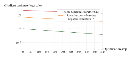
The figure reveals the fundamental tension in BBVI: the score function estimator is maximally general (works for any model and any variational family) but has high variance. The reparameterisation trick (next section) has much lower variance but requires the variational distribution to support a differentiable reparameterisation. For models where the reparameterisation trick applies, it is almost always preferred.
To quantify the difference: in a typical 50-dimensional latent space model, the score function estimator can have variance – times larger than the reparameterised estimator. With sample, the score function estimator often produces gradient estimates whose signal-to-noise ratio is below 1, making optimisation impractical. The reparameterised estimator typically achieves a signal-to-noise ratio above 10 even with a single sample, enabling practical training with minibatch sizes of 32–128.
This variance gap is the primary reason that the VAE (15) uses the reparameterisation trick rather than the score function estimator. For discrete latent variables, where reparameterisation is not available, the variance of BBVI remains a major challenge and an active area of research.
Example 15 (BBVI for Bayesian Logistic Regression).
Consider Bayesian logistic regression with a Gaussian prior on the weights: where is the logistic sigmoid. The posterior has no closed form because the Gaussian prior is not conjugate to the Bernoulli likelihood with a logistic link.
We use a mean-field Gaussian variational family: with . CAVI does not apply (no conjugate exponential family structure).
Using BBVI, each iteration:
Draws samples .
Evaluates .
Computes the score (available in closed form for Gaussians).
Forms the gradient estimate with the optimal baseline and updates .
No model-specific derivations beyond specifying are needed. However, as we shall see in the next section, since the Gaussian family supports reparameterisation, we can do much better.
The Reparameterization Trick
The score function estimator is general but noisy. In this section we develop a dramatically better gradient estimator for the important special case when the variational distribution admits a differentiable reparameterisation, meaning we can express samples from as a deterministic, differentiable transformation of parameter-free noise.
The reparameterisation trick is the technical engine behind the Variational Autoencoder (VAE, 15). It was independently discovered by two groups in 2013–2014, and its impact on the field cannot be overstated: it made end-to-end training of deep latent variable models practical for the first time.
Separating Randomness from Parameters
The fundamental difficulty in computing is that the distribution we are averaging over depends on the parameters . When we draw , the randomness is entangled with the parameters, so we cannot take the gradient inside the expectation directly.
The reparameterisation trick untangles this by expressing the random variable as a deterministic function of and a parameter-free noise variable .
Definition 9 (Reparameterisation).
A distribution admits a reparameterisation if there exists:
a base distribution that does not depend on , and
a differentiable function such that
(DEF)
The reparameterisation converts a stochastic computation (draw from ) into a deterministic computation applied to fixed noise. This seemingly simple change has profound consequences: because is deterministic and differentiable, standard backpropagation can compute through the entire computation, including through the “sampling” step.
The most important example is the Gaussian reparameterisation: (Gauss) where and denotes element-wise multiplication. The noise is drawn from a standard Gaussian that does not depend on ; all the parameter-dependence is in the deterministic transformation .
The Reparameterised Gradient
With the reparameterisation, the expectation transforms: (Transform) Now the distribution inside the expectation does not depend on , so we can freely move the gradient inside: (GRAD) The gradient now flows through and through via the chain rule: (Chain)
Theorem 9 (Reparameterised Gradient Estimator).
Proof.
The unbiasedness follows directly from : the Monte Carlo estimator is the sample mean of , whose expectation under equals .
To build intuition for the lower variance, compare what information each estimator uses. The score function estimator computes : it multiplies the function value (a scalar that can be large and fluctuating) by the score of the variational distribution. The estimator treats as a “reward” signal; it knows the value of at the sampled point but not how would change if moved slightly.
The reparameterised estimator computes : it uses the gradient of with respect to , which is a local linear approximation of 's landscape. This “pathwise” information is far more informative: it tells us not just the value of but the direction in which increases.
More formally, the variance reduction can be understood through the Rao–Blackwell theorem: the reparameterised estimator effectively conditions on more information (the local gradient structure of ) than the score function estimator, and conditioning always reduces variance. A detailed variance comparison can be found in [10].
For the Gaussian case, the reparameterised ELBO gradient has an especially clean form. With and the reparameterisation : (Gradmu) where . These gradients are straightforward to compute via automatic differentiation, requiring only a forward pass (to evaluate ) and a backward pass (to compute ) through the model.
Computational Graph Perspective
The reparameterisation trick has an elegant interpretation in terms of computational graphs, which is how automatic differentiation frameworks (PyTorch, JAX) implement it in practice.
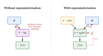
Reparameterisable Distributions
Not every distribution admits a simple reparameterisation. The following table summarises the most commonly used reparameterisable families.
| Distribution | Parameters | Base noise | Transformation |
| Gaussian | |||
| [4pt] Full-cov. Gaussian | |||
| [4pt] Log-normal | |||
| [4pt] Exponential | |||
| [4pt] Gamma | via shape augmentation | implicit | |
| [4pt] von Mises–Fisher | rejection sampling | Householder transform |
Remark 21 (Discrete Distributions).
Discrete distributions (e.g., categorical, Bernoulli) do not admit a differentiable reparameterisation, because the sampling operation involves discrete jumps. Approaches such as the Gumbel-Softmax trick and the straight-through estimator provide biased but useful approximations; we discuss these in Extensions: Handling Non-Reparameterisable Distributions below.
Reparameterisation with Full Covariance
Example 16 (Cholesky Reparameterisation for Multivariate Gaussian).
For a variational distribution with full covariance , we parameterise via its Cholesky factor: , where is lower-triangular with positive diagonal entries. The reparameterisation is: (Cholesky) Then as desired. The variational parameters are , with and having free parameters (lower-triangular entries).
The gradients are: where is the -th standard basis vector. These gradients are propagated through via standard backpropagation, enabling end-to-end gradient-based optimisation of the ELBO with respect to both and .
Connection to Pathwise Gradients
The reparameterisation trick is an instance of a more general idea known as pathwise gradients (or pathwise derivatives) in the operations research and stochastic simulation literature. The key insight is the same: when we can express a random quantity as a deterministic function of a parameter and independent randomness, we can differentiate through the function.
In the notation of stochastic optimisation, for a performance measure where depends on :
The score function approach (likelihood ratio method) differentiates the measure under which we average.
The pathwise approach differentiates the sample path directly.
When both are available, the pathwise approach typically has lower variance because it exploits the local geometry of (via ), while the score function approach only uses information about the density .
Historical Note.
The reparameterisation trick for variational inference was independently proposed by Kingma and Welling [11] (in the context of the VAE) and by Rezende, Mohamed, and Wierstra [10] (in the context of deep latent Gaussian models), both published in 2014. The underlying idea of pathwise differentiation is much older, appearing in the operations research literature under names like “infinitesimal perturbation analysis” and “pathwise sensitivity analysis.” The contribution of Kingma–Welling and Rezende–Mohamed–Wierstra was to recognise that this classical idea, combined with amortised inference and neural network decoders, could unlock scalable training of deep generative models.
Extensions: Handling Non-Reparameterisable Distributions
For distributions that do not admit exact reparameterisation, most notably discrete distributions, several approximations have been developed:
Gumbel–Softmax / Concrete relaxation. Replace a categorical variable with a continuous relaxation using Gumbel noise: (Gumbel) where is a temperature parameter. As , the samples approach one-hot vectors (hard categorical); for , the samples are continuous and differentiable in .
Straight-through estimator. Use the discrete samples in the forward pass but pretend the rounding operation is the identity in the backward pass. This introduces bias but works surprisingly well in practice.
RELAX and other hybrid estimators. Combine the score function estimator with a learned control variate based on a continuous relaxation, achieving lower variance than either approach alone.
Remark 22 (When to Use Which Gradient Estimator).
As a practical guide:
Continuous latent variables with standard families (Gaussian, log-normal, etc.): use the reparameterisation trick. This is the default in modern VI frameworks.
Discrete latent variables: use the score function estimator with variance reduction, or the Gumbel–Softmax relaxation if a biased but low-variance gradient is acceptable.
Mixture of continuous and discrete: reparameterise the continuous part, use score function for the discrete part (Rao–Blackwellisation).
Complex, non-standard distributions: consider implicit reparameterisation or learned surrogates.
Amortized Variational Inference
All the variational inference methods we have seen so far (CAVI, SVI, BBVI, reparameterised VI) share a common pattern: for each data point , we must optimise variational parameters to approximate the posterior . When the dataset contains data points, this means solving separate optimisation problems, each requiring multiple gradient steps.
For a dataset of modest size, this is feasible. But what happens when or ? And what about new data points not seen during training; do we need to run optimisation from scratch for each one?
Amortized inference answers both questions with a single idea: instead of optimising separately for each , train a shared function (typically a neural network) that maps any directly to the variational parameters in a single forward pass.
From Per-Instance to Amortized
Definition 10 (Amortized Inference).
In amortized variational inference, the variational distribution for a data point is parameterised as (DEF) where is an inference network (also called an encoder or recognition network) with parameters , and is the space of variational parameters (e.g., means and variances of a Gaussian).
For example, if , then the inference network outputs , a mean vector and a log-standard-deviation vector, both computed from via a neural network with shared parameters .
The key insight is one of cost amortisation:
1.3
Per-instance VI Amortized VI Parameters
(one per data point) (shared) Cost per new forward pass Training optimise each separately train once
Once is trained, computing the approximate posterior for a new data point (never seen during training) requires only a single forward pass through the network, with no iterative optimisation. This is the “amortisation”: the cost of learning to do inference is paid once during training, and then inference for any input is essentially free.
The term “amortisation” comes from accounting: a large upfront cost (training the network) is spread over many future uses (inference for each data point). Just as a factory invests in machinery that produces many units cheaply, amortised inference invests in a neural network that produces many approximate posteriors cheaply.
Remark 23 (Amortised Inference in the Brain).
There is a fascinating analogy to biological perception. When you see a face, you do not solve an optimisation problem from scratch to infer the 3D shape, lighting, and identity; your visual cortex has been “trained” (through years of visual experience) to map retinal images directly to perceptual interpretations. This is amortised inference in the brain: the cost of learning is paid during development, and perception at test time is fast and feedforward. The Helmholtz machine, a precursor to the VAE proposed by Hinton and Dayan in the 1990s, was explicitly motivated by this analogy.
The Amortised ELBO
The ELBO for amortized inference over a dataset is: (ELBO) where denotes the generative model parameters. We maximise jointly over (inference network) and (generative model) using stochastic gradient ascent, with the reparameterisation trick (The Reparameterization Trick) to estimate the gradients through the sampling.
The Amortization Gap
Amortised inference trades optimality for speed. A single neural network cannot perfectly approximate the optimal variational parameters for every possible input, so it must generalise across inputs, and this generalisation introduces a systematic approximation error.
Definition 11 (Amortization Gap).
The amortization gap for data point is the difference between the optimal per-instance ELBO and the amortised ELBO: (Amortgap)
Proposition 11 (Amortised ELBO is Looser).
The amortised ELBO is bounded above by the per-instance optimal ELBO: (Bound) with the first inequality strict whenever does not equal the per-instance optimal . The total amortization gap for the dataset is .
Proof.
The per-instance ELBO is maximised at . The amortised ELBO evaluates this objective at , which in general differs from . Since is the maximiser, . The second inequality holds because the ELBO is always a lower bound on the log-evidence.
The amortization gap has several sources:
Limited network capacity. The inference network may not be expressive enough to represent the mapping exactly. For example, if the optimal mapping is highly nonlinear but is a shallow network, it will approximate poorly in some regions of input space.
Training data coverage. The network is trained on a finite dataset and must generalise to unseen inputs. In regions of input space poorly represented in the training data, the amortised parameters may be suboptimal.
Multi-modality. If the true posterior is multi-modal for some inputs, the mean-field Gaussian output of a standard inference network cannot capture this structure, regardless of network capacity.
In practice, the amortization gap is typically small for well-designed models: less than a few nats per data point. It can be diagnosed by comparing the amortised ELBO against a locally refined ELBO (as in semi-amortised inference, below).
Semi-Amortized Inference
A natural compromise between per-instance optimisation and full amortisation is semi-amortized inference: use the amortised output as an initialisation for a few steps of local iterative refinement. This combines the speed of amortisation (a good initialisation in one forward pass) with the accuracy of per-instance optimisation (a few gradient steps close the amortization gap).
Concretely:
Compute via the inference network.
For (typically –):
Use as the final variational parameters.
This can be seen as “test-time compute” for inference: spending more computation per data point to get a tighter ELBO.
Amortization and VAEs
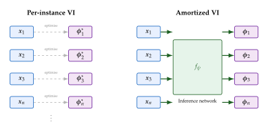
The connection to Variational Autoencoders (15) is now immediate. In a VAE:
The generative model is a deep latent variable model with a neural network decoder.
The approximate posterior is amortised via a neural network encoder (the inference network).
The ELBO is optimised jointly over and using the reparameterisation trick from The Reparameterization Trick.
Thus the VAE encoder is precisely an amortised inference network: it implements , mapping each input to the parameters of a Gaussian approximate posterior in a single forward pass.
Insight.
Amortization: Pay Once, Infer Forever. Amortised inference invests computation during training to learn a mapping from data to posteriors. Once trained, inference for any new data point, even one never seen before, costs only a single forward pass through the network. This is the key enabler that makes variational inference practical for large-scale deep generative models.
The tradeoff is the amortisation gap: the inference network cannot be optimal for every input. In practice, this gap is small for well-trained models with sufficiently expressive encoder architectures, and it can always be reduced by semi-amortised refinement.
Example: Amortized Inference for a Latent Variable Model
Example 17 (Amortised Inference for a Simple Generative Model).
Consider the following latent variable model for 1D data: where is the sigmoid function and are the generative model parameters.
Per-instance approach. For each , we would initialise and run gradient ascent on . With data points and 100 gradient steps per point, this requires gradient evaluations per epoch.
Amortised approach. Define an inference network as a small MLP (e.g., two hidden layers with 64 units). The ELBO becomes: In each training step, we sample a minibatch of data points, draw one noise sample per data point (reparameterisation trick), compute the ELBO gradient with respect to jointly, and update. After training, instantly produces the approximate posterior for any new .
The Road to Deep Generative Models
Let us pause and survey the path we have traversed in this chapter. We began with the fundamental inference problem: computing the posterior . We formulated variational inference as an optimisation problem, minimising over a tractable family, and derived the ELBO as the objective.
The journey from classical to modern VI can be summarised as a sequence of generalisations, each removing a limitation of the previous method:
1.3
Method Limitation Removed Remaining Limitation CAVI (starting point) Requires full data pass;
conjugate models only Variational EM Separates inference from parameter learning Still requires full data pass SVI Subsamples data for scalability Requires conjugate exponential families BBVI Works for any model (score function gradient) High variance gradients Reparameterisation Low-variance gradients Requires differentiable reparameterisation Amortised VI inference per data point Amortisation gap
The combination of amortised inference, the reparameterisation trick, and stochastic minibatch training gives us the VAE (15), the first practical framework for training deep latent variable models at scale. In the next sections, we push further: normalizing flows enrich the variational family beyond mean-field Gaussians, importance-weighted bounds tighten the ELBO, and natural gradients exploit the geometry of the variational distribution for faster convergence.
Remark 24 (The Variational Inference Toolkit).
A practitioner choosing a VI method should consider:
Is the model conjugate? If yes, CAVI or SVI give fast, closed-form updates.
Is the dataset large? If yes, use stochastic methods (SVI, BBVI, or reparameterised VI with minibatches).
Is the variational distribution reparameterisable? If yes, use the reparameterisation trick for low-variance gradients. If not (e.g., discrete latent variables), use BBVI with variance reduction.
Do you need inference for new data at test time? If yes, use amortised inference (an inference network).
Is the mean-field assumption too restrictive? If yes, consider normalising flows or structured variational families (covered in the next sections).
Modern probabilistic programming frameworks such as Pyro (built on PyTorch) and NumPyro (built on JAX) implement all of these methods, allowing the practitioner to mix and match components as needed.
Normalizing Flows for Richer Posteriors
The variational families considered so far (mean-field factorizations, Mean-Field Variational Inference; exponential-family conditionals, Exponential Families and Conjugacy; and even full-covariance Gaussians) impose strong structural assumptions on the approximate posterior. A mean-field Gaussian, for instance, can never capture correlations between latent dimensions, while a full-covariance Gaussian cannot represent multimodality or skewness. When the true posterior exhibits such features, these families introduce an irreducible approximation gap: the ELBO remains strictly below regardless of optimization quality.
Normalizing flows address this limitation by constructing rich, flexible variational families through the composition of simple invertible transformations. The core idea is deceptively simple: start with a tractable base distribution (e.g., a standard Gaussian) and transform it through a sequence of invertible maps to obtain a complex distribution capable of matching intricate posterior geometries.
Change of Variables via Invertible Maps
Let be a smooth, invertible (i.e., diffeomorphic) mapping. If and , then the density of is given by the change of variables formula: (COV) Taking logarithms yields the key identity: (LOG COV) The Jacobian determinant measures how locally stretches or compresses volume, adjusting the density accordingly.
Composing Flows
A single invertible transformation may not be expressive enough. The power of normalizing flows comes from composition: given a sequence of diffeomorphisms , define (FLOW Chain) By iterating the change-of-variables formula, the log-density of the final iterate decomposes as: (FLOW LOG Density) where for . Each transformation may have its own learnable parameters.
Key Idea.
Flows trade computation for expressiveness. Each invertible layer adds to computational cost (depending on the architecture) but strictly increases the capacity of the variational family. With enough layers, flows can in principle approximate any distribution, offering a systematic way to close the approximation gap in the ELBO.
ELBO with Normalizing Flows
Substituting the flow density into the standard ELBO (The Evidence Lower Bound), we obtain: (FLOW ELBO) where is the Jacobian of the -th transformation. The first term encourages the transformed samples to land in high-probability regions under the model; the second and third terms together represent the entropy of the flow distribution, preventing collapse.
Since is a deterministic function of , all expectations are over : we sample , push it through the flow, and evaluate the objective. Gradients flow back through the entire chain via the reparameterization trick (The Reparameterization Trick).
Planar Flows
The simplest flow architecture, introduced by Rezende and Mohamed [23], uses planar transformations: (Planar) where , , and is a smooth activation function (typically ). This transformation adds a perturbation in the direction whose magnitude depends on the projection of onto . Geometrically, it contracts or expands the density along hyperplanes .
The key computational advantage of planar flows is the efficient Jacobian determinant.
Proposition 12 (Planar Flow Jacobian).
Proof.
The Jacobian matrix of is This has the form with and . By the matrix determinant lemma,
For the transformation to be invertible, we require , which imposes the constraint . When , this is enforced by reparameterizing so that [23].
Radial Flows
While planar flows warp the density along hyperplanes, radial flows create contractions and expansions around a reference point : (Radial) where and are scalar parameters. The Jacobian determinant can likewise be computed in : (Radial DET) Radial flows are naturally suited to creating or removing modes, since they can concentrate or disperse density radially.
Beyond Simple Flows
Planar and radial flows have limited per-layer expressiveness (each adds only a single degree of freedom to the density shape). In practice, many layers are needed for complex posteriors. More powerful architectures have been developed that achieve a better balance between expressiveness and computational cost:
RealNVP (Dinh et al. [12]): uses affine coupling layers with triangular Jacobians, yielding determinant computation and exact inversion.
Masked Autoregressive Flows (MAF) (Papamakarios et al. [13]): autoregressive transformations with triangular Jacobians. Density evaluation is efficient but sampling requires sequential passes.
Inverse Autoregressive Flows (IAF) (Kingma et al. [14]): the inverse of MAF, enabling efficient sampling at the cost of slower density evaluation, which is ideal for variational inference where sampling is the bottleneck.
We defer a comprehensive treatment of these architectures to the normalizing flows chapter; here we focus on flows as a tool for enriching variational posteriors.
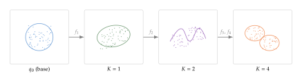
Example 18 (Flow Posterior for a Banana Distribution).
Consider the “banana-shaped” posterior that arises in many hierarchical models, characterized by strong nonlinear correlations. A standard Gaussian cannot capture the curvature, leading to a poor ELBO.
Applying planar flows with activations to a diagonal Gaussian base: with jointly optimized parameters , the flow posterior successfully captures the nonlinear correlation structure. The ELBO gap, measured against a long-run MCMC estimate of , decreases from 3.2 nats (diagonal Gaussian) to 0.15 nats (8-layer flow).
Proposition 13 (Universal Approximation of Flows).
Let be a continuous target density on with finite second moments, and let . For any , there exists a finite composition of smooth invertible maps such that the resulting density satisfies
The proof relies on the fact that smooth diffeomorphisms are dense in the space of measure-preserving maps (in the appropriate topology) [24]. In practice, the number of layers required may be large, and optimization may not find the global optimum, so the approximation guarantee is primarily of theoretical interest.
Insight.
Flows as systematic bias reduction. In the variational inference framework, the approximation error has two components: approximation error (the best in the family is still far from ) and optimization error (we fail to find the best ). Normalizing flows directly attack the approximation error by enlarging the variational family, at the cost of increasing the optimization challenge.
Importance Weighted Bounds
An orthogonal strategy for tightening the ELBO does not change the variational family at all but instead uses multiple samples from to form a tighter lower bound on . The importance weighted autoencoder (IWAE) bound, introduced by Burda et al. [7], achieves this through a simple application of importance sampling.
The IWAE Objective
Draw independent samples from and define the importance weights: (IW Weights) The importance weighted ELBO with samples is: (IWAE Bound) where the expectation is over . Note that recovers the standard ELBO.
The Tightness Hierarchy
The central theoretical result for the IWAE bound is that more importance samples always yield a tighter bound.
Theorem 10 (IWAE Tightness Hierarchy).
For any : (IWAE Hierarchy) Moreover, as .
Proof.
Upper bound. Each importance weight satisfies , so . By Jensen's inequality (since is concave):
Monotonicity. Write and . We can express as a mixture: Since is concave, we have for any realization: Taking expectations and using the fact that the samples are exchangeable, we get , whence: where the last inequality uses (which holds by induction, with the base case being trivial).
Consistency. By the strong law of large numbers, almost surely, so a.s. Dominated convergence (the is bounded above by and the lower bound follows from integrability of ) gives .
Bias Analysis
A Taylor expansion reveals the rate at which the IWAE bound approaches : (IWAE BIAS) Thus the gap closes at rate , and the gap itself is proportional to the relative variance of the importance weights. If is close to , the weights are nearly constant, the variance is small, and even moderate suffices.
The Signal-to-Noise Ratio Problem
While increasing tightens the bound, Rainforth et al. [25] discovered a surprising counterpoint: the gradient signal for the inference network (encoder) deteriorates as grows.
Theorem 11 (SNR Degradation).
Let denote the parameters of the inference network . The signal-to-noise ratio of the IWAE gradient estimator for satisfies: (IWAE SNR)
This result reveals a fundamental tension:
Tighter bound: larger reduces the gap to , helping the generative model ;
Noisier encoder gradient: larger reduces the SNR for , hurting the inference network .
Caution.
More importance samples tighten the bound but may hurt the encoder. Using a very large in the IWAE objective produces a tighter bound on , which benefits the decoder/generative model. However, the encoder gradients become increasingly dominated by noise, potentially leading to a poorly trained inference network. In practice, moderate values ( to ) often work best.
Gradient Computation
The gradient of the IWAE objective with respect to both model parameters and inference parameters can be written using self-normalized importance weights: (IWAE GRAD) are the normalized importance weights. This shows that the IWAE gradient is a weighted combination of per-sample ELBO gradients, with weights proportional to the importance ratios.
Tucker et al. [26] proposed the doubly reparameterized gradient estimator, which modifies the gradient computation to reduce variance without increasing bias. The key insight is to stop gradients through the normalized weights while still obtaining an unbiased estimator, achieving better SNR properties for the encoder.
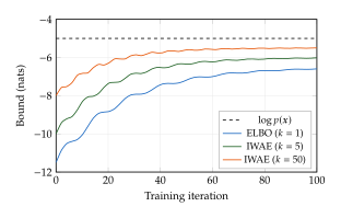
Stein Variational Gradient Descent
All methods discussed so far represent the approximate posterior through a parametric distribution . An entirely different philosophy is to represent the posterior as a collection of particles that are iteratively transported toward high-probability regions of while maintaining diversity. Stein Variational Gradient Descent (SVGD), introduced by Liu and Wang [6], achieves this by combining ideas from Stein's method, kernel methods, and variational inference into an elegant, deterministic update rule.
Stein's Identity and the Stein Operator
The foundation of SVGD is Stein's identity, which characterizes a distribution through an integral condition involving its score function .
Definition 12 (Stein Operator).
Let be a smooth density on and let be a smooth vector-valued test function. The Stein operator applied to is: (Stein Operator) where denotes the divergence.
Lemma 2 (Stein's Identity).
If is a smooth density on and is a smooth test function such that as (boundary condition), then: (Stein Identity)
Proof.
Expanding the trace: where we used and the product rule for divergence. By the divergence theorem, this integral equals the boundary flux , which vanishes by the boundary condition.
The crucial observation is that Stein's identity holds for drawn from any sufficiently regular function class. If for some , then . This motivates using the maximum violation as a discrepancy measure.
Kernelized Stein Discrepancy
To obtain a tractable discrepancy, we restrict to lie in a reproducing kernel Hilbert space (RKHS) with kernel .
Definition 13 (Kernelized Stein Discrepancy).
The kernelized Stein discrepancy (KSD) between and is: (KSD)
By the representer theorem in RKHS, the optimal test function admits a closed-form solution: (KSD Optimal) This function represents the direction of steepest descent for the KL divergence in the space of distributions, as measured by the RKHS norm.
The SVGD Update Rule
Given particles representing the current approximation to , SVGD updates them simultaneously: (SVGD Update) where is the step size. The update has a beautiful interpretation as the sum of two forces:
Attractive force: drives each particle toward high-probability regions, weighted by kernel similarity. When is large (particles are close), particle is strongly influenced by the gradient at particle .
Repulsive force: pushes particles apart, preventing them from collapsing onto a single mode. For an RBF kernel , this term pushes away from nearby particles.
Remark 25.
When , the repulsive term vanishes and SVGD reduces to standard gradient ascent on , yielding a MAP estimate. The multi-particle nature of SVGD is essential for representing uncertainty.
Algorithm 6.
SVGD Algorithm
Input: Target score (up to a constant), kernel , step sizes , number of particles .
Initialize: (e.g., ).
For until convergence: enumerate[(a)]
Compute the kernel matrix: for all .
Compute the score at each particle: .
For each particle , compute the SVGD direction:
Update: . enumerate
Return: particles .
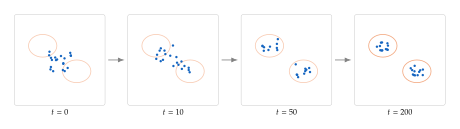
Theoretical Foundation
The SVGD update can be understood as a discretization of a continuous gradient flow on the space of probability distributions.
Theorem 12 (SVGD as KL Gradient Flow).
In the limit of infinitely many particles () and infinitesimal step size (), SVGD implements the gradient flow of in the space of probability distributions, as measured in the RKHS norm. Specifically, the density of the particles at time evolves according to: (SVGD Gradient FLOW) where is the optimal RKHS perturbation , and this dynamics decreases at the fastest rate among all perturbations of unit RKHS norm.
This theorem connects SVGD to the theory of Wasserstein gradient flows, providing a rigorous justification for the particle updates. In practice, the finite-particle approximation introduces bias, and the quality of the approximation depends on both the number of particles and the choice of kernel.
Comparison with MCMC
SVGD occupies an interesting middle ground between variational inference and Markov chain Monte Carlo (MCMC):
| Property | VI (parametric) | SVGD | MCMC |
| Updates | Deterministic | Deterministic | Stochastic |
| Representation | Parameters | Particles | Samples |
| Multimodality | Difficult | Natural | Natural |
| Convergence | Optimization | Optimization | Mixing |
| Asymptotic bias | Yes (family) | No | No |
Example 19 (Bayesian Logistic Regression with SVGD).
Consider binary classification with , , and a logistic likelihood: The unnormalized log-posterior is: SVGD with particles and an RBF kernel , where is set to the median pairwise distance (the median heuristic), provides both a point prediction (particle mean) and uncertainty estimates (particle spread) without any parametric assumptions on the posterior shape.
Insight.
SVGD: the best of both worlds. SVGD combines the computational efficiency of variational methods (deterministic updates, no rejection steps) with the flexibility of particle-based methods (no parametric assumptions, natural handling of multimodality). The kernel controls the trade-off: a wide kernel encourages exploration, while a narrow kernel promotes exploitation.
Natural Gradient Variational Inference
Standard gradient-based optimization of the ELBO treats the variational parameters as living in Euclidean space: the steepest-ascent direction is simply . But parameterizes a probability distribution , and Euclidean geometry is a poor match for the space of distributions. Two parameter vectors and that are close in Euclidean norm may correspond to distributions that are far apart in KL divergence, and vice versa.
The natural gradient [27] resolves this mismatch by equipping the parameter space with the Fisher information metric, the unique Riemannian metric that respects the geometry of probability distributions.
The Fisher Information Matrix
Definition 14 (Fisher Information Matrix).
The Fisher information matrix of a parametric family is: (Fisher)
The Fisher matrix is positive semidefinite and, for regular models, positive definite. It defines a local inner product on the parameter space, making it a Riemannian manifold.
For exponential families (Exponential Families and Conjugacy) with natural parameters , the Fisher matrix has a particularly elegant form: (Fisher Expfam) the Hessian of the log-partition function. Since is convex, is always positive semidefinite, confirming its role as a metric.
The Natural Gradient
Definition 15 (Natural Gradient).
The natural gradient of a function with respect to the Fisher information metric is: (DEF)
The natural gradient is the solution to the constrained optimization problem: find the direction that maximizes the linear approximation subject to a fixed step in KL divergence: (Natgrad Constrained) This ensures that each step moves a fixed “distance” in the space of distributions, not in the space of parameters.
Theorem 13 (Parameterization Invariance).
The natural gradient is invariant under smooth reparameterization. If for a diffeomorphism , then the natural gradient update and the corresponding update in -coordinates produce identical trajectories in distribution space.
Proof.
Under the reparameterization , the Fisher matrix transforms as , where is the Jacobian. The Euclidean gradient transforms as . Therefore: Mapping back: , confirming that the induced distribution update is identical.
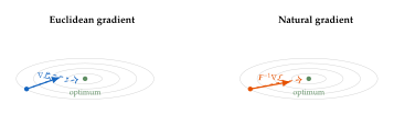
Natural Gradient for Exponential Families
For variational families in the exponential family, the natural gradient has a remarkably simple form. Let denote the mean parameters. Since , the natural gradient update in natural parameters is: (Natgrad Expfam) where is the gradient with respect to the mean parameters. This is the natural gradient expressed purely in terms of mean-parameter gradients, with no explicit matrix inversion required.
The Bayesian Learning Rule
For conjugate exponential-family models with prior and likelihood contributions , the natural gradient update takes the form of the Bayesian learning rule [28]: (BLR) where is a randomly selected data point and is the dataset size. This has a beautiful interpretation: at each step, the natural parameters are a weighted average of the current estimate and a target formed by combining the prior natural parameters with a scaled stochastic estimate of the data contribution.
Remark 26.
The connection to SVI (Stochastic Variational Inference) is now transparent: SVI performs exactly this update. The Robbins–Monro step sizes in SVI are not merely a convergence trick; they arise naturally from the requirement of taking natural gradient steps on the ELBO. SVI was “accidentally” doing the right thing all along.
Practical Methods
Computing the full Fisher matrix is in the number of parameters , which is prohibitive for large models. Several practical approximations have been developed:
Diagonal Fisher: Approximate , reducing storage and inversion to . This is equivalent to using per-parameter adaptive step sizes.
KFAC (Kronecker-factored approximate curvature): For neural networks, approximate the Fisher as a Kronecker product of smaller matrices, one per layer.
VOGN (Variational Online Gauss-Newton): A natural-gradient method for Bayesian neural networks that maintains a diagonal Gaussian posterior over weights [15].
The Bethe Free Energy and Belief Propagation
We now step back from gradient-based optimization and examine variational inference from a broader, unifying perspective. The variational principle for inference, developed systematically by Wainwright and Jordan [29], reveals that essentially all approximate inference methods, including mean field, belief propagation, expectation propagation, and more, can be understood as different approximations to a single optimization problem. This perspective provides deep insight into why methods work (or fail) and suggests principled ways to design new ones.
The Exact Variational Principle
Consider an undirected graphical model (Markov random field) with potential functions for nodes and for edges of a graph . The joint distribution is: (MRF) where collects all natural parameters and collects the sufficient statistics. The log-partition function is the central quantity of interest, since marginals and expectations follow from its derivatives.
The exact variational principle expresses as a convex optimization problem via conjugate duality: (Exact Variational) where is the marginal polytope (the set of all valid marginal vectors realizable by some distribution) and is the entropy written as a function of the marginals. The supremum is attained at , the exact marginals.
This formulation is exact but intractable in general: (i) the marginal polytope has exponentially many constraints, and (ii) the entropy has no closed-form expression in terms of marginals for general graphs.
Mean Field as Inner Approximation
Mean-field VI (Mean-Field Variational Inference) can be recast in this framework as making two approximations:
Inner bound on : restrict to product distributions, which gives a subset . Since we optimize over a smaller set, we obtain a lower bound on .
Exact entropy: the entropy of a product distribution factorizes as , which is exact for the product family.
The mean-field approximation is thus: (MF Variational) The bound is tight only when the true distribution is itself a product (i.e., the graph has no edges).
Belief Propagation and the Bethe Approximation
Belief propagation (BP) takes the opposite approach to mean field, making approximations in a different direction:
Outer relaxation of : replace the marginal polytope with the local polytope: (Local Polytope) which enforces only pairwise marginalization consistency. We always have ; equality holds if and only if is a tree.
Bethe entropy approximation: replace the exact entropy with the Bethe entropy: (Bethe Entropy) where is the marginal entropy of node and is the mutual information of edge .
Definition 16 (Bethe Free Energy).
The Bethe free energy is the negative of the Bethe variational objective: (Bethe FREE Energy) The Bethe approximation to the log-partition function is: (Bethe Approx)
Unlike the mean-field bound, the Bethe approximation is neither an upper nor a lower bound on in general. However, it can be much more accurate than mean field, especially for graphs with weak interactions or high connectivity.
BP Fixed Points and the Bethe Variational Problem
The connection between message-passing algorithms and variational methods is made precise by the following foundational result.
Theorem 14 (BP Fixed Points = Bethe Stationary Points).
Proof sketch.
Write the Lagrangian of the Bethe variational problem with multipliers enforcing the local consistency constraints in . Setting partial derivatives to zero yields stationarity conditions of the form: where are the Lagrange multipliers, and: These are precisely the BP message update equations. Conversely, any BP fixed point defines pseudo-marginals that satisfy the stationarity conditions of the Bethe problem.
Exactness on Trees
Corollary 2 (BP is Exact on Trees).
If is a tree (acyclic graph), then:
The local polytope equals the marginal polytope: .
The Bethe entropy equals the exact entropy: .
BP converges to the unique fixed point, which yields the exact marginals.
This explains the remarkable success of BP on tree-structured models [16] and provides insight into why “loopy” BP (applied to graphs with cycles) often works well in practice: many real-world graphical models have locally tree-like structure.
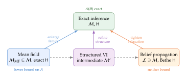
Beyond Bethe: Region-Based Methods
The Bethe approximation uses pairwise interactions. The Kikuchi hierarchy [30] generalizes this to larger regions (clusters of variables), leading to tighter entropy approximations at higher computational cost. The corresponding message-passing algorithms are called generalized belief propagation (GBP). The -th level of the Kikuchi hierarchy uses regions of up to variables and recovers the exact entropy when equals the treewidth of the graph.
Historical Note.
From Pearl's messages to variational free energies. Judea Pearl introduced belief propagation for tree-structured graphical models in 1988 [16], where it provides exact inference. The algorithm was soon applied heuristically to loopy graphs with surprising empirical success. The variational interpretation, connecting BP fixed points to the Bethe free energy, was established by Yedidia, Freeman, and Weiss [17] in 2001, placing loopy BP on firm theoretical footing and opening the door to principled generalizations.
Insight.
All approximate inference methods are variational. The Wainwright–Jordan framework reveals that mean field, belief propagation, expectation propagation, and even MCMC (in a limiting sense) are all solving versions of the same variational problem ; they simply differ in (i) the feasible set (inner or outer approximation to ) and (ii) the entropy approximation . Understanding this unifying structure is essential for choosing and designing inference algorithms.
Variational Inference in Modern Generative Models
Variational inference is not merely a classical technique for approximate Bayesian computation; it is the mathematical engine powering the most successful generative models of the modern era. Variational autoencoders, diffusion models, and even aspects of large language model alignment all rest on variational principles developed in this chapter. We now trace these connections explicitly, demonstrating how the abstract machinery of the ELBO, reparameterization, and amortized inference manifests in concrete generative architectures.
Variational Autoencoders
The variational autoencoder (VAE, 15) is perhaps the most direct application of variational inference. A deep latent variable model specifies: (VAE Model) where and are neural networks. The true posterior is intractable, so we introduce an amortized variational distribution: (VAE Encoder)
The VAE training objective is precisely the ELBO: (VAE ELBO) The first term is the expected reconstruction quality; the second is the KL regularizer pushing the approximate posterior toward the prior (see The Evidence Lower Bound for a detailed derivation).
Key VI innovations in VAEs.
Amortized inference: Rather than optimizing separate variational parameters for each data point , the encoder shares parameters across all data points. This introduces an amortization gap: the amortized posterior may be suboptimal for any individual , but this enables inference at test time.
Reparameterization: The reparameterization trick (The Reparameterization Trick) makes the ELBO differentiable with respect to , enabling joint optimization of encoder and decoder.
-VAE: The modified objective with encourages disentangled representations at the cost of reconstruction quality.
VQ-VAE: Replaces the continuous latent space with discrete codes using vector quantization and the straight-through estimator, sidestepping the KL term entirely.
Diffusion Models as Hierarchical VAEs
Diffusion models (19) can be viewed as hierarchical VAEs with layers of latent variables [31]. The forward (noising) process defines the variational distribution: (DIFF Forward) while the reverse (generative) process is: (DIFF Reverse)
The variational lower bound (ELBO for the Variational Diffusion Model) decomposes as: (DIFF VLB) Crucially, each consistency term is a KL divergence between two Gaussians: the true posterior (available in closed form via Bayes' rule, see Theorem 1) and the learned reverse , making each term analytically tractable.
Remark 27.
The simplified objective used in practice (noise prediction loss) corresponds to a reweighted VLB where the per-timestep weights are uniform rather than the -dependent weights arising from the true VLB. This reweighting improves sample quality at the cost of not optimizing a valid lower bound.
Bayesian Neural Networks
In a Bayesian neural network, we place a prior over the weights and seek the posterior . Variational inference approximates this with , typically a factorized Gaussian: (BNN)
Bayes by Backprop (Blundell et al. [32]) optimizes the ELBO: (Bayes Backprop) using the reparameterization trick: with .
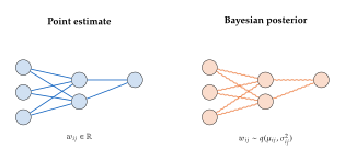
MC-Dropout as implicit VI. Gal and Ghahramani [33] showed that applying dropout at test time (MC-Dropout) is equivalent to approximate variational inference with a specific variational distribution: each weight is either present (with its trained value) or absent (zeroed out), with Bernoulli probability determined by the dropout rate. This provides a practical uncertainty estimate requiring no architectural changes, only keeping dropout active during prediction and averaging over multiple forward passes.
VI and Large Language Models
Variational principles appear in modern large language models in several contexts:
KL regularization in RLHF: Reinforcement learning from human feedback [18] maximizes reward subject to a KL penalty that prevents the policy from deviating too far from a reference model . This is structurally identical to the ELBO, with the reward playing the role of the log-likelihood and the KL penalty playing the role of the regularizer.
Latent reasoning models: Some approaches to improving LLM reasoning introduce latent “thought” variables and optimize a variational bound on , using variational EM to alternately improve the thought generator and the output model.
The Generative Model Family Tree
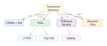
Table 3 summarizes how VI concepts manifest across modern generative model families.
| Model | Variational family | ELBO variant | Key innovation |
| GMM (7) | Categorical + Gaussians | Standard ELBO | EM algorithm |
| VAE (15) | Amortized Gaussian | Standard ELBO | Reparameterization |
| -VAE | Amortized Gaussian | Weighted KL | Disentanglement |
| VQ-VAE | Discrete codes | Commitment loss | Straight-through |
| Diffusion (19) | Fixed forward process | Hierarchical VLB | Noise prediction |
| BNN | Factorized Gaussian | Standard ELBO | Bayes by Backprop |
| LLM (RLHF) | Policy | RewardKL | KL regularization |
Practical Guide and Open Problems
We conclude the chapter with practical guidance for applying variational inference and a survey of open research directions.
Choosing the Right VI Method
The choice of VI algorithm depends on the model structure, dataset size, and desired posterior quality. Figure 21 provides a decision guide.
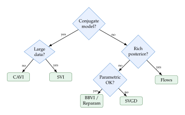
Diagnostics
Monitoring VI convergence and quality requires attention to several indicators:
ELBO monitoring: Plot the ELBO across iterations. A plateau indicates convergence (but possibly to a local optimum). Sudden drops suggest numerical issues.
Posterior predictive checks: Sample , generate synthetic data , and compare distributional properties with the observed data. Systematic discrepancies reveal model or approximation inadequacies.
Comparison to MCMC on small problems: On low-dimensional subproblems or subsets of data, run MCMC to obtain ground-truth posterior summaries. Compare VI marginals, means, and variances to MCMC estimates. Large discrepancies indicate the variational family is too restrictive.
Gradient variance monitoring: For BBVI (Black-Box Variational Inference), monitor the variance of gradient estimates. Excessively high variance indicates the need for better control variates or larger mini-batches.
Common Pitfalls
Mode collapse in mean-field: Mean-field VI minimizes the reverse KL , which is mode-seeking: the optimizer concentrates on a single mode of a multimodal posterior, ignoring others entirely.
Poor initialization: CAVI and gradient-based methods can converge to poor local optima. Multiple random restarts or initialization from simpler models (e.g., initializing from the prior) can mitigate this.
Posterior collapse in VAEs: When the decoder is too powerful, the model learns to ignore the latent variables entirely, with for all (see Posterior Collapse).
Gradient variance in BBVI: The score-function gradient estimator (Black-Box Variational Inference) can have extremely high variance, making optimization impractical without careful variance reduction via control variates and baselines.
Underestimated uncertainty: Variational posteriors, especially mean-field ones, systematically underestimate posterior variance. This can lead to overconfident predictions in downstream tasks.
Open Research Directions
Despite decades of development, variational inference remains an active area of research with several important open problems:
Tighter bounds without SNR degradation: The IWAE bound (Importance Weighted Bounds) tightens monotonically in but degrades encoder gradients. Designing bounds that are simultaneously tight and provide high-quality gradients for all model components remains open.
Better structured variational families: Beyond mean-field and normalizing flows, what are the “right” variational families that balance expressiveness, computational cost, and optimization difficulty? Structured mean-field approaches that exploit graphical model structure are promising but underexplored for deep models.
VI for discrete structures: Most VI methods assume continuous latent variables. Extending reparameterization-style tricks to discrete latent variables (beyond Gumbel-Softmax) remains challenging, with implications for program synthesis, combinatorial optimization, and symbolic reasoning.
Scaling VI to trillion-parameter models: As models grow to hundreds of billions or trillions of parameters, maintaining even a diagonal Gaussian posterior requires doubling the parameter count. Efficient representations of uncertainty at this scale are needed.
Connections to optimal transport: Wasserstein distances and optimal transport maps offer alternative geometries for measuring the discrepancy between and . Replacing KL divergence with Wasserstein-type objectives leads to different algorithms with potentially better properties for multimodal posteriors.
Exercises
Exercise 10 (KL Divergence between Gaussians ).
Let and be univariate Gaussians.
Show that the KL divergence is:
Verify that if and only if and .
Generalize to -dimensional Gaussians and .
Exercise 11 (Forward vs Reverse KL ).
Let be a symmetric bimodal mixture.
Find the Gaussian that minimizes (reverse KL, used in VI). Hint: argue by symmetry and mode-seeking behavior that there are two local optima plus a saddle point.
Find the Gaussian that minimizes (forward KL). Show that and .
Explain qualitatively why the reverse KL selects a single mode while the forward KL covers both modes. Which behavior is preferable for approximate inference?
Exercise 12 (Deriving the ELBO from Jensen's Inequality ).
Starting from the marginal likelihood and an arbitrary distribution :
Multiply and divide by inside the integral.
Apply Jensen's inequality to obtain .
Identify when equality holds.
Exercise 13 (Deriving the ELBO from KL Decomposition ).
Starting from the definition of , show that:
Explain why this immediately implies that the ELBO is a lower bound on .
Exercise 14 (ELBO Tightness ).
Using the decomposition from Exercise 13, prove that the ELBO equals if and only if almost everywhere. Explain why this means the gap between the ELBO and measures the quality of the variational approximation.
Exercise 15 (Mean-Field Optimal Factor ).
Consider the joint distribution and the mean-field factorization .
Derive the optimal holding fixed, using the mean-field update .
Show that is Gaussian. Find its mean and variance.
By symmetry, write down and verify that the mean-field approximation underestimates the correlation between and .
Exercise 16 (CAVI for Bayesian Linear Regression ).
Consider the model , , with priors and .
Derive the CAVI update for .
Derive the CAVI update for .
Write pseudocode for the full CAVI algorithm.
Exercise 17 (CAVI for Bayesian GMM ).
Consider a Bayesian Gaussian mixture model with components: , , with priors and .
Write down the complete-data log-likelihood.
Derive the CAVI update for (a categorical distribution over components).
Derive the CAVI update for (a Gaussian).
Derive the CAVI update for (a Dirichlet).
Explain how these updates relate to the EM algorithm for GMMs (7).
Exercise 18 (CAVI Monotonically Increases the ELBO ).
Prove that each coordinate update in CAVI (Algorithm 1) does not decrease the ELBO. Hint: Show that the CAVI update for factor solves , and that replacing with its optimum can only increase .
Exercise 19 (Gradient of the Log-Partition Function ).
Let be an exponential family distribution.
Show that .
Show that .
Conclude that is convex.
Exercise 20 (Natural Parameter Updates for Conjugate Models ).
Consider a Bayesian model with likelihood from an exponential family with sufficient statistic and a conjugate prior .
Show that the posterior is in the same family with updated natural parameters.
Express the updated parameters in terms of , , and the data sufficient statistics.
Interpret the prior parameters as “pseudo-observations.”
Exercise 21 (Variational EM for a Latent Factor Model ).
Consider the model with , , and .
Write down the ELBO for this model with .
VE-step: Derive the optimal for fixed .
VM-step: Derive the updates for and for fixed .
Show that this recovers probabilistic PCA in the limit.
Exercise 22 (SVI Natural Gradient for LDA ).
In Latent Dirichlet Allocation, each document has topic proportions and each word is drawn from topic with word distribution .
Write down the complete-data log-likelihood.
Identify the global and local variational parameters.
Derive the noisy natural gradient update for the global parameter (the Dirichlet parameter of the variational distribution over topics).
Verify that the SVI update has the form of (BLR).
Exercise 23 (Robbins–Monro Convergence ).
Consider the stochastic approximation iteration , where and the step sizes satisfy , .
Explain intuitively why both conditions are necessary: ensures we can reach any point; ensures the noise averages out.
Verify that satisfies both conditions for .
For the quadratic case with and , prove that in mean square.
Exercise 24 (Score Function Has Zero Expectation ).
Let be a smooth parametric density. Prove that . Hint: Differentiate with respect to and exchange differentiation and integration.
Exercise 25 (BBVI Gradient for Logistic Regression ).
Consider Bayesian logistic regression with and prior .
Write down the ELBO with .
Derive the score function (REINFORCE) gradient estimator for .
Derive the reparameterized gradient estimator.
Discuss the expected variance of each estimator.
Exercise 26 (Optimal Control Variate Coefficient ).
Given a gradient estimator and a control variate with , the variance-reduced estimator is .
Show that is unbiased for any .
Derive the optimal coefficient that minimizes .
Show that the resulting variance reduction is , where is the correlation between and .
Exercise 27 (Reparameterization Trick for Gaussian ).
Let with . Compute :
Analytically, using .
Via the reparameterization trick with , .
Verify that both methods give the same result.
Exercise 28 (Gumbel-Softmax Density ).
The Gumbel-Softmax distribution with temperature and log-probabilities assigns density to (the simplex) via:
Verify that as , the samples approach one-hot vectors (categorical samples).
Show that the density is well-defined on the simplex (integrates to 1).
Explain why the Gumbel-Softmax provides a continuous relaxation of categorical variables that enables the reparameterization trick.
Exercise 29 (Planar Flow Jacobian Determinant ).
For the planar flow :
Compute the Jacobian matrix .
State the matrix determinant lemma: for any invertible and , .
Use the lemma to derive the result .
What constraint on and is needed to ensure invertibility when ?
Exercise 30 (IWAE Bound is Tighter than ELBO ).
Show that the standard ELBO is (the special case ).
Using Jensen's inequality and the concavity of , prove that .
Generalize: show for all .
Construct a simple example (e.g., being jointly Gaussian, ) and numerically compute to verify the hierarchy.
Exercise 31 (Stein's Identity for Smooth Distributions ).
Let be a smooth density on with as .
Prove the univariate Stein identity: for smooth with at the boundaries.
Verify the identity for and .
Extend the proof to using the divergence theorem.
Exercise 32 (SVGD with the RBF Kernel ).
Consider SVGD with the RBF kernel .
Exercise 33 (Natural Gradient for Diagonal Gaussian ).
Let the variational family be with .
Compute the Fisher information matrix . Show that it is block-diagonal between and .
Derive the natural gradient of an objective with respect to and .
Show that the natural gradient with respect to equals the Euclidean gradient scaled by : per-parameter adaptive step sizes.
Compare to the Adam optimizer [19]: what similarities and differences do you observe?
Exercise 34 (BP is Exact on Trees ).
Consider a tree-structured graphical model with pairwise potentials.
Show that for a tree, any collection of pairwise-consistent marginals satisfying corresponds to a valid joint distribution. (This proves for trees.)
Show that for a tree, the Bethe entropy equals the exact joint entropy . Hint: Use the chain rule for entropy along the tree edges.
Conclude that BP computes exact marginals on trees.
Exercise 35 (Diffusion Variational Lower Bound ).
For a diffusion model with steps:
Starting from , derive the decomposition into prior matching, consistency, and reconstruction terms ((DIFF VLB)).
Show that each consistency term is a KL between two Gaussians and derive its closed-form expression.
Explain why the forward process is not learned (unlike in a standard VAE) and how this simplifies optimization.
Exercise 36 (Mean-Field vs Structured VI on a Chain ).
Consider a Markov chain where each , with , .
Compute the exact marginals for .
Apply mean-field VI with and derive the CAVI updates. Run them to convergence and report the resulting marginals.
Apply structured VI with and derive the updates. Compare the resulting marginals with the mean-field solution.
Quantify the approximation error of each method using total variation distance.
Exercise 37 (Implement CAVI for a Bayesian GMM ).
Write detailed pseudocode for CAVI applied to the Bayesian GMM from Exercise 17, including:
Initialization strategy (e.g., from -means or random).
The update loop, specifying the order of updates for , , and .
ELBO computation for convergence monitoring.
A clear specification of all expectations needed (e.g., and ).
Exercise 38 (The Amortization Gap ).
Define the amortization gap as the difference between the amortized ELBO (using ) and the per-instance optimal ELBO (optimizing separately for each ).
Construct a simple example where the amortization gap is nonzero. Hint: consider a model where changes qualitatively for different values (e.g., the posterior is unimodal for some and bimodal for others), and the encoder cannot represent both shapes.
Discuss strategies for reducing the amortization gap (e.g., iterative amortized inference, semi-amortized inference).
Exercise 39 (KL Minimization Equals ELBO Maximization ).
Show that for a fixed model and observed data :
Explain why this equivalence is important: we can optimize the ELBO (which requires only the joint ) instead of the KL (which requires the intractable posterior ).
Does this equivalence hold when is the set of all distributions? What is the solution in that case?
0.60.5pt
The exercises above span the full range of variational inference topics covered in this chapter. Exercises 1–5 test foundational understanding of KL divergence and the ELBO\@; Exercises 6–9 develop fluency with mean-field and CAVI\@; Exercises 10–14 cover exponential families, SVI, and stochastic optimization; Exercises 15–19 address gradient estimation and the reparameterization trick; Exercises 20–21 treat normalizing flows and importance weighting; Exercises 22–24 develop SVGD and natural gradient methods; and Exercises 25–30 connect VI to graphical models, diffusion models, and modern practice.
References
-
On information and sufficiency
BibTeX
@article{kullback1951information, title={On information and sufficiency}, author={Kullback, Solomon and Leibler, Richard A}, journal={The annals of mathematical statistics}, volume={22}, number={1}, pages={79--86}, year={1951}, publisher={Institute of Mathematical Statistics} }Journal article
-
An Introduction to Variational Methods for Graphical Models
BibTeX
@article{jordan1999introduction, title={An Introduction to Variational Methods for Graphical Models}, author={Jordan, Michael I. and Ghahramani, Zoubin and Jaakkola, Tommi S. and Saul, Lawrence K.}, journal={Machine Learning}, volume={37}, number={2}, pages={183--233}, year={1999} }Journal article
-
The Computational Complexity of Probabilistic Inference using Bayesian Belief Networks
BibTeX
@article{cooper1990computational, title={The Computational Complexity of Probabilistic Inference using {Bayesian} Belief Networks}, author={Cooper, Gregory F.}, journal={Artificial Intelligence}, volume={42}, number={2--3}, pages={393--405}, year={1990} }Journal article
-
Divergence Measures and Message Passing
BibTeX
@inproceedings{minka2005divergence, title={Divergence Measures and Message Passing}, author={Minka, Tom}, booktitle={Microsoft Research Technical Report}, year={2005} }Conference paper
-
Variational Message Passing
BibTeX
@article{winn2005variational, title={Variational Message Passing}, author={Winn, John and Bishop, Christopher M.}, journal={Journal of Machine Learning Research}, volume={6}, pages={661--694}, year={2005} }Journal article
-
Stein Variational Gradient Descent: A General Purpose Bayesian Inference Algorithm
BibTeX
@inproceedings{liu2016stein, title={Stein Variational Gradient Descent: A General Purpose {B}ayesian Inference Algorithm}, author={Liu, Qiang and Wang, Dilin}, booktitle={Advances in Neural Information Processing Systems (NeurIPS)}, pages={2378--2386}, year={2016} }Conference paper
-
Importance Weighted Autoencoders
BibTeX
@inproceedings{burda2016importance, title={Importance Weighted Autoencoders}, author={Burda, Yuri and Grosse, Roger and Salakhutdinov, Ruslan}, booktitle={International Conference on Learning Representations (ICLR)}, year={2016} }Conference paper
-
Variational Inference: A Review for Statisticians
BibTeX
@article{blei2017variational, title={Variational Inference: A Review for Statisticians}, author={Blei, David M. and Kucukelbir, Alp and McAuliffe, Jon D.}, journal={Journal of the American Statistical Association}, volume={112}, number={518}, pages={859--877}, year={2017} }Journal article
-
A stochastic approximation method
BibTeX
@Article{robbins1951stochastic, Title = {A stochastic approximation method}, Author = {Robbins, H. and Monro, S.}, Journal = {The Annals of Mathematical Statistics}, Year = {1951}, Pages = {400--407}, Publisher = {JSTOR} }Journal article
-
Stochastic Backpropagation and Approximate Inference in Deep Generative Models
BibTeX
@inproceedings{rezende2014stochastic, title={Stochastic Backpropagation and Approximate Inference in Deep Generative Models}, author={Rezende, Danilo Jimenez and Mohamed, Shakir and Wierstra, Daan}, booktitle={International Conference on Machine Learning}, pages={1278--1286}, year={2014} }Conference paper
-
Auto-Encoding Variational Bayes
BibTeX
@inproceedings{kingma2013auto, title={Auto-Encoding Variational {B}ayes}, author={Kingma, Diederik P and Welling, Max}, booktitle={International Conference on Learning Representations}, year={2014} }Conference paper
-
Density Estimation using Real-NVP
BibTeX
@inproceedings{dinh2017density, title={Density Estimation using {Real-NVP}}, author={Dinh, Laurent and Sohl-Dickstein, Jascha and Bengio, Samy}, booktitle={Proceedings of the International Conference on Learning Representations (ICLR)}, year={2017} }Conference paper
-
Masked Autoregressive Flow for Density Estimation
BibTeX
@inproceedings{papamakarios2017masked, title={Masked Autoregressive Flow for Density Estimation}, author={Papamakarios, George and Pavlakou, Theo and Murray, Iain}, booktitle={Advances in Neural Information Processing Systems}, pages={2338--2347}, year={2017} }Conference paper
-
Improved Variational Inference with Inverse Autoregressive Flow
BibTeX
@inproceedings{kingma2016improved, title={Improved Variational Inference with Inverse Autoregressive Flow}, author={Kingma, Diederik P. and Salimans, Tim and Jozefowicz, Rafal and Chen, Xi and Sutskever, Ilya and Welling, Max}, booktitle={Advances in Neural Information Processing Systems}, pages={4743--4751}, year={2016} }Conference paper
-
Practical Deep Learning with Bayesian Principles
BibTeX
@inproceedings{osawa2019practical, title={Practical Deep Learning with {Bayesian} Principles}, author={Osawa, Kazuki and Swaroop, Siddharth and Khan, Mohammad Emtiyaz and Jain, Anirudh and Eschenhagen, Runa and Turner, Richard E. and Henning, Rio}, booktitle={Advances in Neural Information Processing Systems (NeurIPS)}, year={2019} }Conference paper
-
Probabilistic Reasoning in Intelligent Systems: Networks of Plausible Inference
BibTeX
@book{pearl1988probabilistic, title={Probabilistic Reasoning in Intelligent Systems: Networks of Plausible Inference}, author={Pearl, Judea}, publisher={Morgan Kaufmann}, year={1988} }Book
-
Understanding Belief Propagation and Its Generalizations
BibTeX
@article{yedidia2003understanding, title={Understanding Belief Propagation and Its Generalizations}, author={Yedidia, Jonathan S and Freeman, William T and Weiss, Yair}, journal={Exploring Artificial Intelligence in the New Millennium}, volume={8}, pages={236--239}, year={2003} }Journal article
-
Training Language Models to Follow Instructions with Human Feedback
BibTeX
@article{ouyang2022training, title={Training Language Models to Follow Instructions with Human Feedback}, author={Ouyang, Long and Wu, Jeffrey and Jiang, Xu and Almeida, Diogo and Wainwright, Carroll and Mishkin, Pamela and Zhang, Chong and Agarwal, Sandhini and Slama, Katarina and Ray, Alex and others}, journal={Advances in Neural Information Processing Systems}, volume={35}, pages={27730--27744}, year={2022} }Journal article
-
Adam: A Method for Stochastic Optimization
BibTeX
@article{kingma2015adam, title={Adam: A Method for Stochastic Optimization}, author={Kingma, Diederik P. and Ba, Jimmy}, journal={Proceedings of the International Conference on Learning Representations (ICLR)}, year={2015} }Journal article
-
Stochastic Variational Inference
BibTeX
@article{hoffman2013stochastic, title={Stochastic Variational Inference}, author={Hoffman, Matthew D. and Blei, David M. and Wang, Chong and Paisley, John}, journal={Journal of Machine Learning Research}, volume={14}, pages={1303--1347}, year={2013} }Journal article
-
Black Box Variational Inference
BibTeX
@inproceedings{ranganath2014black, title={Black Box Variational Inference}, author={Ranganath, Rajesh and Gerrish, Sean and Blei, David M.}, booktitle={Proceedings of the International Conference on Artificial Intelligence and Statistics (AISTATS)}, pages={814--822}, year={2014} }Conference paper
-
Simple Statistical Gradient-Following Algorithms for Connectionist Reinforcement Learning
BibTeX
@article{williams1992simple, title={Simple Statistical Gradient-Following Algorithms for Connectionist Reinforcement Learning}, author={Williams, Ronald J.}, journal={Machine Learning}, volume={8}, number={3--4}, pages={229--256}, year={1992} }Journal article
-
Variational Inference with Normalizing Flows
BibTeX
@inproceedings{rezende2015variational, title={Variational Inference with Normalizing Flows}, author={Rezende, Danilo Jimenez and Mohamed, Shakir}, booktitle={International Conference on Machine Learning}, pages={1530--1538}, year={2015} }Conference paper
-
Triangular Transformations of Measures
BibTeX
@article{bogachev2005triangular, title={Triangular Transformations of Measures}, author={Bogachev, Vladimir I. and Kolesnikov, Alexander V. and Medvedev, Kirill V.}, journal={Sbornik: Mathematics}, volume={196}, number={3}, pages={309--335}, year={2005} }Journal article
-
Tighter Variational Bounds are Not Necessarily Better
BibTeX
@inproceedings{rainforth2018tighter, title={Tighter Variational Bounds are Not Necessarily Better}, author={Rainforth, Tom and Kosiorek, Adam R. and Le, Tuan Anh and Maddison, Chris J. and Igl, Maximilian and Wood, Frank and Teh, Yee Whye}, booktitle={Proceedings of the International Conference on Machine Learning (ICML)}, pages={4277--4285}, year={2018} }Conference paper
-
Doubly Reparameterized Gradient Estimators for Monte Carlo Objectives
BibTeX
@inproceedings{tucker2019doubly, title={Doubly Reparameterized Gradient Estimators for {M}onte {C}arlo Objectives}, author={Tucker, George and Lawson, Dieterich and Gu, Shixiang and Maddison, Chris J.}, booktitle={International Conference on Learning Representations (ICLR)}, year={2019} }Conference paper
-
Natural Gradient Works Efficiently in Learning
BibTeX
@article{amari1998natural, title={Natural Gradient Works Efficiently in Learning}, author={Amari, Shun-ichi}, journal={Neural Computation}, volume={10}, number={2}, pages={251--276}, year={1998} }Journal article
-
The Bayesian Learning Rule
BibTeX
@article{khan2021bayesian, title={The {Bayesian} Learning Rule}, author={Khan, Mohammad Emtiyaz and Rue, H{\aa}vard}, journal={Journal of Machine Learning Research}, volume={24}, number={281}, pages={1--46}, year={2023} }Journal article
-
Graphical Models, Exponential Families, and Variational Inference
BibTeX
@article{wainwright2008graphical, title={Graphical Models, Exponential Families, and Variational Inference}, author={Wainwright, Martin J. and Jordan, Michael I.}, journal={Foundations and Trends in Machine Learning}, volume={1}, number={1--2}, pages={1--305}, year={2008} }Journal article
-
Constructing Free-Energy Approximations and Generalized Belief Propagation Algorithms
BibTeX
@article{yedidia2005constructing, title={Constructing Free-Energy Approximations and Generalized Belief Propagation Algorithms}, author={Yedidia, Jonathan S. and Freeman, William T. and Weiss, Yair}, journal={IEEE Transactions on Information Theory}, volume={51}, number={7}, pages={2282--2312}, year={2005} }Journal article
-
Variational Diffusion Models
BibTeX
@inproceedings{kingma2021variational, title={Variational Diffusion Models}, author={Kingma, Diederik and Salimans, Tim and Poole, Ben and Ho, Jonathan}, booktitle={Advances in Neural Information Processing Systems}, volume={34}, pages={21696--21707}, year={2021} }Conference paper
-
Weight Uncertainty in Neural Networks
BibTeX
@inproceedings{blundell2015weight, title={Weight Uncertainty in Neural Networks}, author={Blundell, Charles and Cornebise, Julien and Kavukcuoglu, Koray and Wierstra, Daan}, booktitle={Proceedings of the International Conference on Machine Learning (ICML)}, pages={1613--1622}, year={2015} }Conference paper
-
Dropout as a Bayesian Approximation: Representing Model Uncertainty in Deep Learning
BibTeX
@inproceedings{gal2016dropout, title={Dropout as a {B}ayesian Approximation: Representing Model Uncertainty in Deep Learning}, author={Gal, Yarin and Ghahramani, Zoubin}, booktitle={Proceedings of the International Conference on Machine Learning (ICML)}, pages={1050--1059}, year={2016} }Conference paper