7 Gaussian Mixture Models

Real-world data is seldom generated by a single, simple distribution. Heights in a population mixing adults and children are bimodal. Pixel intensities in a natural image form multiple clusters. Gene expression levels across cell types follow distinct modes. Whenever the data-generating process has multiple regimes, a single Gaussian is a poor model.

The Gaussian mixture model (GMM) is the simplest and most instructive way to handle multimodality: model the density as a weighted sum of several Gaussian components. Despite its simplicity, the GMM already exhibits many of the phenomena that recur in modern generative modelling: latent variables, intractable likelihoods, the EM algorithm, and the tension between model capacity and computational tractability.

Historical Note.

The idea of finite mixtures dates back to Karl Pearson's 1894 paper [1], in which he decomposed the distribution of crab forehead-to-body ratios into two Gaussian components, inventing the method of moments along the way. The modern EM algorithm for fitting mixtures was formalised by Dempster, Laird, and Rubin in their landmark 1977 paper [2], which unified a wide variety of iterative procedures under a single framework. The EM algorithm remains the standard tool for fitting mixture models and is the conceptual ancestor of the variational methods used in VAEs and diffusion models.

Why Mixtures?

Example 1 (Old Faithful Geyser).

The Old Faithful geyser in Yellowstone erupts at intervals that are clearly bimodal: sometimes around 55 minutes, sometimes around 80 minutes. A single Gaussian centred near 68 minutes would place high density where no data exists and miss both modes. A mixture of two Gaussians captures each mode separately and assigns low density to the gap between them.

More generally, a single Gaussian $𝒩 (𝝁, 𝚺)$ can only represent a unimodal, ellipsoidal density. It cannot capture:

Multiple modes (clusters, subpopulations).
Skewness or heavy tails.
Complex shapes (banana-shaped, ring-shaped densities).

A mixture of Gaussians can, in principle, approximate any continuous density to arbitrary accuracy, given enough components (Theorem Theorem 3).

The Gaussian Mixture Model

Definition 1 (Gaussian Mixture Model).

A Gaussian mixture model with $K$ components in $ℝ^{d}$ is a probability density of the form (GMM) $\begin{matrix} p (𝒙) = \sum_{k = 1}^{K} π_{k} 𝒩 (𝒙 | 𝝁_{k}, 𝚺_{k}), \end{matrix}$ where:

$π_{k} \geq 0$ are the mixing weights (or mixing coefficients), satisfying $\sum_{k = 1}^{K} π_{k} = 1$ .
$𝝁_{k} \in ℝ^{d}$ is the mean of the $k$ -th component.
$𝚺_{k} \in ℝ^{d \times d}$ is the (symmetric, positive-definite) covariance matrix of the $k$ -th component.
$𝒩 (𝒙 | 𝝁, 𝚺) = (2 π)^{- d / 2} | 𝚺 |^{- 1 / 2} \exp (- \frac{1}{2} (𝒙 - 𝝁)^{𝖳} 𝚺^{- 1} (𝒙 - 𝝁))$ is the multivariate Gaussian density.

The full parameter set is $θ = {π_{k}, 𝝁_{k}, 𝚺_{k}}_{k = 1}^{K}$ .

The Latent Variable Interpretation

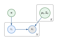
A GMM has an elegant interpretation as a latent variable model, connecting it directly to the PGM framework of Chapter 6.

Definition 2 (GMM as a Latent Variable Model).

Introduce a discrete latent variable $z \in {1, \dots, K}$ indicating which component generated a given observation: (GEN) $\begin{matrix} z & \sim Categorical (π_{1}, \dots, π_{K}), \\ 𝒙 | z = k & \sim 𝒩 (𝝁_{k}, 𝚺_{k}) . \end{matrix}$ Marginalising over $z$ recovers the mixture density : $p (𝒙) = \sum_{k = 1}^{K} P (z = k) p (𝒙 | z = k) = \sum_{k = 1}^{K} π_{k} 𝒩 (𝒙 | 𝝁_{k}, 𝚺_{k}) .$

Plate diagram for the Gaussian mixture model (cf. Chapter 6). Each data point

𝒙_{i}

depends on its latent assignment

z_{i}

and the component parameters

(𝝁_{k}, 𝚺_{k})

. Shaded nodes are observed.

Key Idea.

The GMM is a generative model: it specifies a complete probabilistic story for how data is generated. To sample a new data point, we:

Draw a component index $z \sim Categorical (𝝅)$ .
Draw $𝒙 \sim 𝒩 (𝝁_{z}, 𝚺_{z})$ .

This two-step procedure is the simplest instance of the ancestral sampling pattern that recurs in VAEs ( $𝒛 \to 𝒙$ ), autoregressive models ( $x_{1} \to x_{2} \to \dots$ ), and diffusion models ( $𝒙_{T} \to 𝒙_{T - 1} \to \dots \to 𝒙_{0}$ ).

Geometry of Gaussian Mixtures

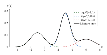
To build intuition, let us visualise what GMMs look like.

A 1D Gaussian mixture with

K = 3

components. Dashed curves show the weighted components

π_{k} 𝒩 (x | μ_{k}, σ_{k}^{2})

; the solid black curve is their sum, the mixture density. The mixture captures three distinct modes.

Example 2 (Reading the 1D Mixture).

In Figure fig:gmm:1d, the three components have:

Component	$π_{k}$	$μ_{k}$	$σ_{k}^{2}$
1 (green)	0.3	$- 1$	1.0
2 (blue)	0.5	3	0.5
3 (red)	0.2	6	1.5

The blue component is the tallest and narrowest (large

π

, small

σ^{2}

). The red component is the broadest (large

σ^{2}

) but has the smallest weight. The mixture density has three modes, a shoulder between the green and blue peaks, and a long right tail contributed by the red component.

Remark 1 (Effect of Covariance Structure in 2D).

In two or more dimensions, each component's covariance matrix $𝚺_{k}$ controls the shape of its density contours:

Spherical ( $𝚺_{k} = σ_{k}^{2} I$ ): circular contours. Fewest parameters ( $K$ scalars).
Diagonal ( $𝚺_{k} = diag (σ_{k 1}^{2}, \dots, σ_{k d}^{2})$ ): axis-aligned ellipses. $K d$ parameters.
Full ( $𝚺_{k}$ unconstrained): arbitrarily oriented ellipses. $K d (d + 1) / 2$ parameters.

Choosing the covariance type is a bias–variance trade-off: more flexible shapes fit data better but require more parameters and are more prone to overfitting.

Maximum Likelihood Estimation

Given $N$ i.i.d. observations $𝒟 = {𝒙_{1}, \dots, 𝒙_{N}}$ , we want to find the parameters $θ$ that best explain the data. The log-likelihood is

(LL) $\begin{matrix} ℓ (θ) = \sum_{i = 1}^{N} \log p (𝒙_{i}; θ) = \sum_{i = 1}^{N} \log \sum_{k = 1}^{K} π_{k} 𝒩 (𝒙_{i} | 𝝁_{k}, 𝚺_{k}) . \end{matrix}$

Caution.

The log-likelihood contains a log of a sum, which prevents it from decomposing into per-component terms. This is fundamentally different from the “complete-data” log-likelihood where each $z_{i}$ is known (Proposition Proposition 2). Direct gradient-based optimisation is possible but awkward; the EM algorithm provides an elegant alternative.

The Singularity Problem

Proposition 1 (MLE Singularity).

The GMM log-likelihood is unbounded above. Specifically, if we set $𝝁_{k} = 𝒙_{j}$ for some data point $𝒙_{j}$ and let $𝚺_{k} \to 𝟎$ , then $𝒩 (𝒙_{j} | 𝝁_{k}, 𝚺_{k}) \to \infty$ , so $ℓ (θ) \to + \infty$ .

Proof.

For the $j$ -th term in the log-likelihood: $\log p (𝒙_{j}) \geq \log [π_{k} 𝒩 (𝒙_{j} | 𝒙_{j}, σ^{2} I)] = \log π_{k} - \frac{d}{2} \log (2 π σ^{2}) .$ As $σ^{2} \to 0$ , this diverges to $+ \infty$ .

∎

Example 3 (Singularity in Practice).

Imagine fitting $K = 2$ components to data ${1, 2, 3, 4, 5}$ . If we set $μ_{1} = 3$ (exactly on a data point) and $σ_{1}^{2} \to 0$ , the likelihood shoots to infinity. This is a degenerate solution: the component has “collapsed” onto a single point. In practice, this is avoided by:

Adding a regularisation term (e.g. $𝚺_{k} + ϵ I$ ).
Using Bayesian priors (e.g. an inverse-Wishart prior on $𝚺_{k}$ ).
Monitoring for near-singular components and resetting them.

The EM Algorithm for GMMs

The EM algorithm, introduced in Chapter 6 (Definition Definition 9), has a particularly clean closed-form instantiation for GMMs.

Complete-Data Log-Likelihood

If we knew the latent assignments $z_{1}, \dots, z_{N}$ , the log-likelihood would decompose:

Proposition 2 (Complete-Data Log-Likelihood).

With observed $(𝒙_{i}, z_{i})$ pairs, the complete-data log-likelihood is (LL) $\begin{matrix} ℓ_{c} (θ) = \sum_{i = 1}^{N} \sum_{k = 1}^{K} 𝟙 [z_{i} = k] [\log π_{k} + \log 𝒩 (𝒙_{i} | 𝝁_{k}, 𝚺_{k})], \end{matrix}$ which decomposes over components: each $π_{k}$ , $𝝁_{k}$ , $𝚺_{k}$ can be estimated independently.

Insight.

The fundamental trick of EM is: since we don't know $z_{i}$ , we replace the hard indicator $𝟙 [z_{i} = k]$ with its soft expectation $γ_{i k} = P (z_{i} = k | 𝒙_{i}; θ^{(t)})$ , the responsibility of component $k$ for data point $i$ . This turns the intractable problem (log-of-sum) into a tractable one (sum-of-logs, weighted by responsibilities).

E-Step: Computing Responsibilities

Definition 3 (Responsibility).

The responsibility of component $k$ for observation $𝒙_{i}$ is the posterior probability: (Responsibility) $\begin{matrix} γ_{i k} \overset{def}{=} P (z_{i} = k | 𝒙_{i}; θ^{(t)}) = \frac{π_{k}^{(t)} 𝒩 (𝒙_{i} | 𝝁_{k}^{(t)}, 𝚺_{k}^{(t)})}{\sum_{j = 1}^{K} π_{j}^{(t)} 𝒩 (𝒙_{i} | 𝝁_{j}^{(t)}, 𝚺_{j}^{(t)})} . \end{matrix}$

This is simply Bayes' theorem: the prior $P (z_{i} = k) = π_{k}$ is updated by the likelihood $p (𝒙_{i} | z_{i} = k)$ to give the posterior.

Example 4 (Computing Responsibilities by Hand).

Consider $K = 2$ components in 1D with current parameters: $π_{1} = π_{2} = 0.5$ , $μ_{1} = 0$ , $μ_{2} = 4$ , $σ_{1}^{2} = σ_{2}^{2} = 1$ . For a data point $x = 1$ : $\begin{matrix} 𝒩 (1 | 0, 1) & = \frac{1}{\sqrt{2 π}} e^{- 1 / 2} \approx 0.2420, \\ 𝒩 (1 | 4, 1) & = \frac{1}{\sqrt{2 π}} e^{- 9 / 2} \approx 0.0044. \end{matrix}$ So the responsibilities are: $γ_{1} = \frac{0.5 \times 0.2420}{0.5 \times 0.2420 + 0.5 \times 0.0044} = \frac{0.1210}{0.1232} \approx 0.982, γ_{2} \approx 0.018.$ Component 1 “claims” 98.2% of the responsibility for $x = 1$ ; it is much more likely that this point came from the component centred at $0$ than the one centred at $4$ .

M-Step: Updating Parameters

Given the responsibilities, we update each parameter by maximising the expected complete-data log-likelihood $Q (θ, θ^{(t)}) = 𝔼_{z | 𝒙; θ^{(t)}} [ℓ_{c} (θ)]$ .

Theorem 1 (M-Step Updates for GMMs).

Define the effective count $N_{k} = \sum_{i = 1}^{N} γ_{i k}$ . The M-step updates are: (PI) $\begin{matrix} π_{k}^{(t + 1)} & = \frac{N_{k}}{N}, \\ 𝝁_{k}^{(t + 1)} & = \frac{1}{N_{k}} \sum_{i = 1}^{N} γ_{i k} 𝒙_{i}, \\ 𝚺_{k}^{(t + 1)} & = \frac{1}{N_{k}} \sum_{i = 1}^{N} γ_{i k} (𝒙_{i} - 𝝁_{k}^{(t + 1)}) {(𝒙_{i} - 𝝁_{k}^{(t + 1)})}^{𝖳} . \end{matrix}$

Proof.

We derive each update by differentiating the expected complete-data log-likelihood.

Mean. Differentiating $Q$ with respect to $𝝁_{k}$ : $\frac{\partial Q}{\partial 𝝁_{k}} = \sum_{i = 1}^{N} γ_{i k} 𝚺_{k}^{- 1} (𝒙_{i} - 𝝁_{k}) = 𝟎 ⟹ 𝝁_{k} = \frac{\sum_{i} γ_{i k} 𝒙_{i}}{\sum_{i} γ_{i k}} .$

Covariance. Similarly, differentiating $Q$ with respect to $𝚺_{k}^{- 1}$ and using the identity $\frac{\partial}{\partial 𝚺^{- 1}} \log | 𝚺^{- 1} | = 𝚺$ yields .

Mixing weights. We maximise $Q$ subject to $\sum_{k} π_{k} = 1$ using a Lagrange multiplier: $\frac{\partial}{\partial π_{k}} [\sum_{i} \sum_{j} γ_{i j} \log π_{j} + λ (1 - \sum_{j} π_{j})] = 0 ⟹ \frac{N_{k}}{π_{k}} = λ ⟹ π_{k} = \frac{N_{k}}{N} .$

∎

Remark 2 (Intuition for the M-Step).

Each update has a beautiful interpretation:

$π_{k} = N_{k} / N$ : the mixing weight is the fraction of data softly assigned to component $k$ .
$𝝁_{k}$ : the mean is the responsibility-weighted average of the data.
$𝚺_{k}$ : the covariance is the responsibility-weighted scatter around the new mean.

Compare with the hard-assignment case (plain averaging over cluster members): EM simply replaces “member of cluster $k$ ” with “has responsibility $γ_{i k}$ for cluster $k$ ”.

The Complete EM Algorithm

Algorithm 1 (EM for Gaussian Mixture Models).

Input: Data ${𝒙_{1}, \dots, 𝒙_{N}}$ , number of components $K$ , convergence threshold $ϵ$ .

Initialise $π_{k}^{(0)}, 𝝁_{k}^{(0)}, 𝚺_{k}^{(0)}$ for $k = 1, \dots, K$ .

repeat

E-step: For each $i, k$ , compute responsibility $γ_{i k}$ via .
M-step: Update $π_{k}, 𝝁_{k}, 𝚺_{k}$ via –.
Evaluate: Compute log-likelihood $ℓ (θ)$ via .

until $| ℓ (θ^{(t + 1)}) - ℓ (θ^{(t)}) | < ϵ$ .

Output: Fitted parameters $θ^{*} = {π_{k}, 𝝁_{k}, 𝚺_{k}}_{k = 1}^{K}$ .

A Worked Numerical Example

Example 5 (One Iteration of EM in 1D).

Consider $K = 2$ with data ${- 1, 0, 4, 5}$ and initial parameters: $π_{1} = π_{2} = 0.5$ , $μ_{1} = 0$ , $μ_{2} = 3$ , $σ_{1}^{2} = σ_{2}^{2} = 1$ .

E-step. Compute the Gaussian density at each point for each component, then responsibilities:

$x_{i}$	$𝒩 (x_{i} \| 0, 1)$	$𝒩 (x_{i} \| 3, 1)$	$γ_{i 1}$	$γ_{i 2}$
$- 1$	0.2420	0.0001	0.9996	0.0004
$0$	0.3989	0.0044	0.9891	0.0109
$4$	0.0001	0.2420	0.0004	0.9996
$5$	0.0000	0.0540	0.0000	1.0000

M-step. Effective counts: $N_{1} \approx 1.989$ , $N_{2} \approx 2.011$ . $\begin{matrix} π_{1}^{(1)} & \approx 0.497, π_{2}^{(1)} \approx 0.503, \\ μ_{1}^{(1)} & = \frac{0.9996 \cdot (- 1) + 0.9891 \cdot 0 + 0.0004 \cdot 4 + 0.0000 \cdot 5}{1.989} \approx - 0.502, \\ μ_{2}^{(1)} & \approx \frac{0.0004 \cdot (- 1) + 0.0109 \cdot 0 + 0.9996 \cdot 4 + 1.0000 \cdot 5}{2.011} \approx 4.487. \end{matrix}$ The means have moved toward the two natural clusters ${- 1, 0}$ and ${4, 5}$ . Further iterations would converge to $μ_{1} \approx - 0.5$ and $μ_{2} \approx 4.5$ .

Convergence Properties

Theorem 2 (Monotone Convergence of EM).

Each EM iteration increases (or leaves unchanged) the observed-data log-likelihood: $ℓ (θ^{(t + 1)}) \geq ℓ (θ^{(t)}) .$

Proof.

By Jensen's inequality, the E-step constructs a lower bound $Q (θ, θ^{(t)}) + const$ on $ℓ (θ)$ that is tight at $θ = θ^{(t)}$ . The M-step maximises this bound, so $ℓ (θ^{(t + 1)}) \geq Q (θ^{(t + 1)}, θ^{(t)}) + const \geq Q (θ^{(t)}, θ^{(t)}) + const = ℓ (θ^{(t)})$ . See Chapter 6, Proposition Proposition 3 for the general statement.

∎

Caution.

EM converges to a local maximum, not a global one. The solution depends on initialisation. Practical strategies include:

$k$ -means initialisation: run $k$ -means first and use the cluster centroids as initial means.
$k$ -means++: a smarter seeding that spreads initial centres apart.
Multiple restarts: run EM several times and keep the solution with the highest log-likelihood.

EM as Coordinate Ascent on the ELBO

The EM algorithm has a beautiful interpretation as coordinate ascent on the evidence lower bound (ELBO), which provides the bridge to variational inference (Chapter 8).

Proposition 3 (Log-Likelihood Decomposition).

For any distribution $q (z_{i})$ over latent variables: (Decompose) $\begin{matrix} \log p (𝒙_{i}; θ) = \underset{ELBO (θ, q)}{\underset{⏟}{\sum_{k = 1}^{K} q (z_{i} = k) \log \frac{p (𝒙_{i}, z_{i} = k; θ)}{q (z_{i} = k)}}} + \underset{\geq 0}{\underset{⏟}{𝖣_{KL} (q (z_{i}) ‖ p (z_{i} | 𝒙_{i}; θ))}} . \end{matrix}$ Since the KL divergence is non-negative, the ELBO is a lower bound on the log-likelihood.

Insight.

The two EM steps correspond to alternating maximisation of the ELBO:

E-step: fix $θ$ , maximise ELBO over $q$ . The optimum is $q^{*} (z_{i}) = p (z_{i} | 𝒙_{i}; θ)$ (the responsibilities), which makes the KL term zero and the ELBO equal to the log-likelihood.
M-step: fix $q$ , maximise ELBO over $θ$ . This is equivalent to maximising the expected complete-data log-likelihood $Q (θ, θ^{(t)})$ .

For GMMs, the E-step is tractable (closed-form responsibilities). For more complex models like VAEs, the E-step is intractable, so we restrict $q$ to a parametric family and optimise with gradient descent; this is variational inference.

Relationship to $k$ -Means

The popular $k$ -means clustering algorithm is a special case of GMM-EM.

Proposition 4 ( $k$ -Means as a Limiting Case).

Consider a GMM with $K$ components sharing the same isotropic covariance $𝚺_{k} = σ^{2} I$ for all $k$ . In the limit $σ^{2} \to 0$ :

The responsibilities become hard assignments: $γ_{i k} \to 𝟙 [k = {arg min}_{j} ‖ 𝒙_{i} - 𝝁_{j} ‖^{2}]$ .
The M-step mean update becomes the centroid: $𝝁_{k} = \frac{1}{| C_{k} |} \sum_{i \in C_{k}} 𝒙_{i}$ .

This is exactly the $k$ -means algorithm.

Remark 3 (Soft vs. Hard Assignments).

Points near a cluster boundary get split responsibility in GMM-EM (e.g. $γ_{i 1} = 0.6$ , $γ_{i 2} = 0.4$ ), whereas $k$ -means assigns them entirely to the nearest centroid. This soft assignment makes GMMs more robust to overlapping clusters, at the cost of slower convergence and a more complex model.

Model Selection: Choosing $K$

How do we choose the number of components $K$ ? Increasing $K$ always increases the log-likelihood (more parameters means better fit), so we need a regularised criterion.

Definition 4 (Information Criteria).

Two common model selection criteria are: (BIC) $\begin{matrix} BIC & = - 2 ℓ (\hat{θ}) + p \log N, \\ AIC & = - 2 ℓ (\hat{θ}) + 2 p, \end{matrix}$ where $ℓ (\hat{θ})$ is the maximised log-likelihood, $p$ is the number of free parameters, and $N$ is the number of data points. Lower is better: these criteria trade off goodness-of-fit against model complexity.

Example 6 (Parameter Count for a GMM).

For a GMM with $K$ components in $ℝ^{d}$ and full covariance matrices, the number of free parameters is: $p = \underset{mixing weights}{\underset{⏟}{(K - 1)}} + \underset{means}{\underset{⏟}{K d}} + \underset{covariances}{\underset{⏟}{K \cdot \frac{d (d + 1)}{2}}} = K (\frac{d (d + 1)}{2} + d + 1) - 1.$ For $d = 10$ and $K = 5$ : $p = 5 (55 + 10 + 1) - 1 = 329$ parameters. This grows quadratically in $d$ , a foretaste of the curse of dimensionality.

Remark 4 (BIC vs. AIC).

The BIC penalises complexity more heavily (penalty $\propto \log N$ ) and tends to select simpler models. It is consistent: as $N \to \infty$ , it selects the true $K$ with probability 1 (assuming the data truly comes from a finite mixture). The AIC penalises less (penalty $\propto 2$ ) and tends to select more complex models, which can give better predictive performance. In practice, the BIC is the more common choice for selecting the number of mixture components.

GMMs as Generative Models

GMMs are not just a clustering tool; they are fully specified generative models. Once we have estimated $θ$ , we can generate new data by ancestral sampling (see the Key Idea box in Section The Latent Variable Interpretation).

Algorithm 2 (Sampling from a GMM).

Input: Fitted parameters ${π_{k}, 𝝁_{k}, 𝚺_{k}}_{k = 1}^{K}$ , number of samples $M$ .

for $m = 1, \dots, M$ :

Draw $z^{(m)} \sim Categorical (π_{1}, \dots, π_{K})$ .
Compute Cholesky factor $𝐋_{k} = chol (𝚺_{z^{(m)}})$ .
Draw $𝝐^{(m)} \sim 𝒩 (0, I)$ .
Set $𝒙^{(m)} = 𝝁_{z^{(m)}} + 𝐋_{z^{(m)}} 𝝐^{(m)}$ .

return ${𝒙^{(1)}, \dots, 𝒙^{(M)}}$ .

Example 7 (GMM as Image Generator?).

Suppose we have $N = 60,000$ images of handwritten digits (MNIST), each flattened to $d = 784$ dimensions. We fit a GMM with $K = 50$ components. Sampling from this GMM produces new 784-dimensional vectors that we can reshape into $28 \times 28$ images.

The results are blurry and noisy. Each component mean $𝝁_{k}$ typically looks like a blurred average of similar digits, and samples from that component add Gaussian noise to this average. The model cannot produce sharp, realistic digits because:

It models individual pixel statistics, not spatial structure.
The Gaussian assumption produces “fuzzy” samples, since real images have sharp edges and discrete intensities.
Modelling $784$ -dimensional full covariances requires $\sim 300,000$ parameters per component.

Universal Density Approximation

Despite these practical limitations, GMMs have a remarkable theoretical property:

Theorem 3 (GMM as Universal Approximator).

Any continuous probability density on $ℝ^{d}$ can be approximated arbitrarily well (in the sense of $L^{1}$ convergence) by a Gaussian mixture with sufficiently many components $K$ .

Proof sketch.

Cover the support of the target density $p^{*}$ with small hypercubes. In each hypercube, approximate $p^{*}$ by a Gaussian whose mean is the centre of the cube and whose covariance is proportional to the cube volume. As the cubes shrink, the approximation converges to $p^{*}$ in $L^{1}$ .

∎

Remark 5 (Theory vs. Practice).

The universal approximation theorem tells us GMMs are theoretically expressive enough. But the required $K$ may be astronomically large (exponential in $d$ ), and fitting that many components from finite data is hopeless. This is the familiar curse of dimensionality, the same gap between existence and practicality that motivates deep generative models.

Challenges of GMMs for Generation

Challenge	GMM Limitation	Deep Model Solution
Curse of dimensionality	$O (K d^{2})$ parameters in total	Learned low-dim. manifold (VAE)
No spatial structure	Flat vector, no pixel locality	CNNs, U-Nets
Blurry samples	Gaussian noise in pixel space	Adversarial loss (GAN), score matching
Mode coverage	Needs $K$ per mode; $K$ fixed	Continuous latent space
Scalability	$O (N K d^{2})$ per EM iteration	SGD on mini-batches
Discrete structure	Cannot model sharp edges	Nonlinear decoders

Challenges of GMMs as generative models and how deep models address them.

Key Idea.

The GMM is the simplest generative model: latent variable $z$ selects a mode, and then $𝒙$ is drawn from that mode. Every subsequent generative model we study can be seen as addressing one or more of the GMM's limitations:

VAEs replace the discrete $z \in {1, \dots, K}$ with a continuous latent $𝒛 \in ℝ^{m}$ and use a neural network decoder instead of a fixed Gaussian.
Normalising flows make the mapping $𝒛 \to 𝒙$ invertible so the density $p (𝒙)$ is tractable.
GANs abandon the explicit density entirely and directly learn a mapping $𝒛 \to 𝒙$ .
Diffusion models use a hierarchy of latent variables (a long chain) instead of a single $z$ .

In this sense, the GMM is the ancestor of all deep generative models.

When GMMs Are the Right Choice

Despite their limitations for high-dimensional generation, GMMs remain an excellent choice in many settings:

Example 8 (Good Use Cases for GMMs).

Density estimation in low-to-moderate dimensions ( $d ≲ 50$ ): financial returns, sensor data, scientific measurements.
Clustering with uncertainty: unlike $k$ -means, GMMs give soft assignments and cluster shapes (ellipses, not spheres).
Anomaly detection: a point $𝒙$ with $p (𝒙) < τ$ is flagged as anomalous.
Speaker verification: the “i-vector + GMM-UBM” pipeline was the standard in automatic speaker recognition for decades.
Initialisation for deep models: GMM clustering of latent codes is used in some VAE variants.
Mixture density networks (Section Mixture Density Networks): neural networks that output GMM parameters, combining the expressiveness of deep models with the interpretability of mixtures.

Beyond Basic GMMs

Bayesian GMMs and the Dirichlet Process

A key limitation of standard GMMs is that $K$ must be chosen in advance. Bayesian nonparametric methods address this.

Definition 5 (Dirichlet Process Mixture Model).

A Dirichlet process mixture model (DPMM) places a Dirichlet process prior $DP (α, G_{0})$ on the mixing distribution, where $α > 0$ is the concentration parameter and $G_{0}$ is the base measure. This allows the number of active components to grow with the data:

Small $α$ : few components (data is simple).
Large $α$ : many components (data is complex).

The “Chinese restaurant process” provides an intuitive construction: the $(N + 1)$ -th customer joins existing table $k$ with probability $\propto N_{k}$ , or starts a new table with probability $\propto α$ .

Remark 6 (Practical Use).

DPMMs avoid the model selection problem entirely but are more expensive to fit (typically via Gibbs sampling or variational inference). They are useful when the number of clusters is unknown and may grow with data size, e.g. in topic modelling, population genetics, or astronomical source detection.

Mixture Density Networks

A powerful extension combines GMMs with neural networks:

Definition 6 (Mixture Density Network).

A mixture density network (MDN) [3] is a neural network that takes input $𝒙$ and outputs the parameters of a conditional GMM: $p (𝒚 | 𝒙) = \sum_{k = 1}^{K} π_{k} (𝒙) 𝒩 (𝒚 | 𝝁_{k} (𝒙), 𝚺_{k} (𝒙)),$ where $π_{k} (𝒙)$ , $𝝁_{k} (𝒙)$ , $𝚺_{k} (𝒙)$ are all output by the network (with appropriate constraints: softmax for $π_{k}$ , positive-definiteness for $𝚺_{k}$ ).

Insight.

MDNs are a bridge between classical GMMs and modern deep generative models. In fact, the decoder of a VAE with a mixture-of-Gaussians output can be viewed as an MDN conditioned on the latent code $𝒛$ . MDNs are particularly useful for modelling multi-valued functions, e.g. inverse kinematics (multiple joint configurations for one end-effector position) or probabilistic weather forecasting (multiple plausible trajectories).

Chapter Summary

A Gaussian mixture model represents a density as $p (𝒙) = \sum_{k} π_{k} 𝒩 (𝒙 | 𝝁_{k}, 𝚺_{k})$ , a weighted sum of Gaussian components.
The latent variable interpretation ( $z \to 𝒙$ ) connects GMMs to the PGM framework and ancestral sampling.
The EM algorithm alternates between computing responsibilities (E-step) and updating parameters (M-step); it monotonically increases the log-likelihood and converges to a local optimum.
EM can be understood as coordinate ascent on the ELBO, bridging to variational inference.
$k$ -means is a special case of GMM-EM in the hard-assignment limit.
The BIC/AIC provide principled model selection for choosing $K$ .
GMMs are fully specified generative models, but struggle in high dimensions due to the curse of dimensionality and lack of spatial structure. They are the conceptual ancestor of all deep generative models.
Extensions include Bayesian nonparametrics (DPMM) and mixture density networks (MDNs).

In the next chapter, we study variational inference, the framework that generalises the EM algorithm to models where the E-step is intractable, enabling VAEs and modern deep generative models.

Exercises

Exercise 1 (EM by Hand).

Consider a 1D GMM with $K = 2$ , initial parameters $π_{1} = π_{2} = 0.5$ , $μ_{1} = 0$ , $μ_{2} = 3$ , $σ_{1}^{2} = σ_{2}^{2} = 1$ , and data ${- 1, 0, 4, 5}$ .

(a)
Perform one E-step: compute $γ_{i k}$ for each data point and component.
(b)
Perform one M-step: compute updated $π_{k}$ , $μ_{k}$ , $σ_{k}^{2}$ .
(c)
Compute the log-likelihood before and after this iteration and verify it increased.

Exercise 2 (Deriving the M-Step).

Starting from the expected complete-data log-likelihood $Q (θ, θ^{(t)}) = \sum_{i = 1}^{N} \sum_{k = 1}^{K} γ_{i k} [\log π_{k} + \log 𝒩 (𝒙_{i} | 𝝁_{k}, 𝚺_{k})],$

(a)
Derive the M-step update for $𝝁_{k}$ by setting $\partial Q / \partial 𝝁_{k} = 0$ .
(b)
Derive the M-step update for $𝚺_{k}$ .
(c)
Use Lagrange multipliers to derive the update for $π_{k}$ subject to $\sum_{k} π_{k} = 1$ .

Exercise 3 (Monotonicity of EM).

Prove that EM never decreases the observed-data log-likelihood. Hint: Use Jensen's inequality and the decomposition $\log p (𝒙) = ELBO + 𝖣_{KL}$ .

Exercise 4 ( $k$ -Means as GMM Limit).

Consider a GMM with shared isotropic covariance $𝚺_{k} = σ^{2} I$ for all $k$ .

(a)
Show that as $σ^{2} \to 0$ , the responsibilities become hard assignments.
(b)
Show the M-step mean update reduces to the $k$ -means centroid rule.
(c)
Give a dataset where soft EM assignments produce qualitatively different clusters than $k$ -means.

Exercise 5 (Initialisation and Local Optima).

(a)
Construct a 1D example where poor EM initialisation converges to a suboptimal local maximum.
(b)
Explain why multiple random restarts help.
(c)
Describe $k$ -means++ and explain why it provides good initialisation for EM.

Exercise 6 (Singularity Analysis).

(a)
Show that setting $𝝁_{k} = 𝒙_{j}$ and $𝚺_{k} \to 𝟎$ causes $ℓ (θ) \to + \infty$ .
(b)
Why doesn't this happen in practice with reasonable initialisation?
(c)
Propose two regularisation strategies and explain their effect.

Exercise 7 (BIC Model Selection).

Generate $N = 500$ samples from a 2D GMM with $K^{*} = 3$ components.

(a)
Fit GMMs with $K = 1, 2, \dots, 8$ and compute BIC for each.
(b)
Plot BIC vs. $K$ . Does the minimum occur at $K = 3$ ?
(c)
Repeat with $N = 50$ . Is model selection harder with less data?

Exercise 8 (GMM Sampling and Evaluation).

Fit a GMM with $K = 10$ components (full covariance) to the MNIST training set (flattened to $d = 784$ ).

(a)
Sample 100 images and visualise them. Describe the quality.
(b)
Compute the log-likelihood on the test set.
(c)
Repeat with $K = 50$ and $K = 200$ . Does the log-likelihood improve? Do the samples improve visually?
(d)
Discuss why increasing $K$ eventually fails to improve sample quality despite improving likelihood.

Exercise 9 (ELBO Decomposition).

Starting from the identity $\log p (𝒙; θ) = ELBO (θ, q) + 𝖣_{KL} (q (z) ‖ p (z | 𝒙; θ))$ :

(a)
Derive this decomposition from first principles.
(b)
Show that the E-step sets the KL term to zero.
(c)
Show that the M-step increases the ELBO by maximising over $θ$ .
(d)
Explain in your own words why this means EM can only increase (or maintain) the log-likelihood.

Exercise 10 (Curse of Dimensionality for GMMs).

(a)
Compute the number of free parameters for a GMM with $K = 20$ and full covariance in $d = 100$ .
(b)
How many data points $N$ would you need for reliable estimation? (A common rule of thumb is $N ≫ p$ .)
(c)
Suggest two strategies to reduce the parameter count (e.g. diagonal covariances, PCA preprocessing) and discuss their trade-offs.
(d)
Explain why deep generative models like VAEs handle $d = 784$ or $d = 3072$ while GMMs cannot.

Exercise 11 (GMM as Universal Approximator).

(a)
Construct a GMM that approximates a Uniform $[0,1]$ density using $K$ equally-weighted, equally-spaced components with variance $σ^{2} = 1 / (12 K^{2})$ . Plot the approximation for $K = 3, 10, 50$ .
(b)
How does the $L^{1}$ approximation error scale with $K$ ?
(c)
Repeat for a bimodal density. How does the required $K$ grow with the distance between modes?

Exercise 12 (Mixture Density Network).

Consider predicting $y \in ℝ$ from $x \in ℝ$ where the true relationship is $y = x + 0.3 \sin (2 π x) + ϵ$ with $ϵ \sim 0.5 𝒩 (- 1, {0.1}^{2}) + 0.5 𝒩 (1, {0.1}^{2})$ (bimodal noise).

(a)
Why would a standard neural network with MSE loss fail to capture the bimodal conditional $p (y | x)$ ?
(b)
Design an MDN with $K = 2$ Gaussian components. What are the output dimensions of the network?
(c)
Write the negative log-likelihood loss for training.
(d)
After training, how would you sample from $p (y | x)$ for a given $x$ ?

Exercise 13 (GMM for Anomaly Detection).

Fit a GMM with $K = 5$ to a dataset of “normal” 2D data points.

(a)
Explain how to use $p (𝒙)$ as an anomaly score.
(b)
What threshold $τ$ would you choose, and how?
(c)
A new data point $𝒙^{*}$ has $γ_{i k} \approx 0$ for all $k$ but $p (𝒙^{*})$ is not extremely low. How is this possible? (Hint: consider the tails of the Gaussian.)
(d)
Suggest a modification to make GMM-based anomaly detection more robust.

Exercise 14 (From GMM to VAE).

Trace the conceptual path from GMM to VAE:

(a)
In a GMM, the latent variable $z$ is discrete. What happens if we replace it with a continuous $𝒛 \sim 𝒩 (0, I)$ ?
(b)
The GMM decoder is $p (𝒙 | z = k) = 𝒩 (𝝁_{k}, 𝚺_{k})$ . What does the VAE replace this with?
(c)
The GMM E-step computes $P (z | 𝒙)$ exactly. Why can't we do this for the continuous-latent model, and what does the VAE do instead?
(d)
Summarise: what are the three key changes from GMM to VAE?

References

Contributions to the Mathematical Theory of Evolution

Karl Pearson

Philosophical Transactions of the Royal Society of London A, vol. 185, pp. 71-110 · 1894

BibTeX

@article{pearson1894contributions,
  title={Contributions to the Mathematical Theory of Evolution},
  author={Pearson, Karl},
  journal={Philosophical Transactions of the Royal Society of London A},
  volume={185},
  pages={71--110},
  year={1894}
}

Journal article

Maximum Likelihood from Incomplete Data via the EM Algorithm

Arthur P Dempster, Nan M Laird, Donald B Rubin

Journal of the Royal Statistical Society: Series B, vol. 39, no. 1, pp. 1-38 · 1977

BibTeX

@article{dempster1977maximum,
  title={Maximum Likelihood from Incomplete Data via the {EM} Algorithm},
  author={Dempster, Arthur P and Laird, Nan M and Rubin, Donald B},
  journal={Journal of the Royal Statistical Society: Series B},
  volume={39},
  number={1},
  pages={1--38},
  year={1977}
}

Journal article

Mixture Density Networks

Christopher M Bishop

Aston University Technical Report NCRG/94/004 · 1994

BibTeX

@article{bishop1994mixture,
  title={Mixture Density Networks},
  author={Bishop, Christopher M},
  journal={Aston University Technical Report NCRG/94/004},
  year={1994}
}

Journal article

← 6 Probabilistic Graphical Models 8 Variational Inference →

7 Gaussian Mixture Models

Why Mixtures?

The Gaussian Mixture Model

The Latent Variable Interpretation

Geometry of Gaussian Mixtures

Maximum Likelihood Estimation

The Singularity Problem

The EM Algorithm for GMMs

Complete-Data Log-Likelihood

E-Step: Computing Responsibilities

M-Step: Updating Parameters

The Complete EM Algorithm

A Worked Numerical Example

Convergence Properties

EM as Coordinate Ascent on the ELBO

Relationship to k-Means

Model Selection: Choosing K

GMMs as Generative Models

Universal Density Approximation

Challenges of GMMs for Generation

When GMMs Are the Right Choice

Beyond Basic GMMs

Bayesian GMMs and the Dirichlet Process

Mixture Density Networks

Chapter Summary

Exercises

References

Relationship to $k$ -Means

Model Selection: Choosing $K$