6 Probabilistic Graphical Models

A joint distribution over $n$ binary variables requires $2^{n} - 1$ free parameters, a number that grows astronomically with $n$ . For just 30 variables this is already over a billion. Clearly, writing down or learning such a table is hopeless without further structure.

Probabilistic graphical models (PGMs) solve this problem by encoding conditional independence assumptions in the language of graphs. Every node is a random variable; edges (or their absence) declare which variables directly influence one another. The graph structure implies a factorisation of the joint distribution into a product of small, local terms, each involving only a variable and its immediate neighbours.

Key Idea.

A graphical model uses a graph to compactly represent a high-dimensional joint distribution.

Nodes = random variables.
Edges = direct statistical dependencies.
Missing edges = conditional independences that enable factorisation.

The graph is not merely a visualisation aid: it is a precise mathematical object that determines which factorisations are valid and which inference algorithms are tractable.

Why should we care about PGMs in a book on generative modelling? Because every major generative model family can be expressed as a graphical model:

VAEs are directed latent-variable models (section PGMs as the Language of Generative Models).
Autoregressive models are Bayesian networks with a chain factorisation.
Diffusion models are hierarchical directed models with a fixed forward process.
Energy-based models are undirected graphical models.

Understanding PGMs gives us a unified language for reasoning about the structure, training, and inference of all these models.

Historical Note.

The idea of using graphs to represent statistical relationships dates back to the geneticist Sewall Wright, who introduced path diagrams in 1921 to study causal relationships in genetics [1]. The modern theory of Bayesian networks was developed by Judea Pearl in the 1980s [2], culminating in his 2011 Turing Award “for fundamental contributions to artificial intelligence through the development of a calculus for probabilistic and causal reasoning.” The parallel theory of undirected models traces to statistical physics (the Ising model, 1925) and was formalised in statistics by Hammersley and Clifford in 1971 [3]. The comprehensive treatment by Koller and Friedman [4] unified both traditions.

Directed Graphical Models: Bayesian Networks

A Bayesian network¹ is a directed acyclic graph (DAG) in which each node $X_{i}$ has a conditional probability distribution (CPD) given its parents.

Definition 1 (Bayesian Network).

A Bayesian network is a pair $(𝒢, Θ)$ where:

$𝒢 = (𝒱, ℰ)$ is a directed acyclic graph (DAG) with nodes $𝒱 = {X_{1}, \dots, X_{n}}$ .
$Θ = {P (X_{i} | Pa (X_{i}))}_{i = 1}^{n}$ is a collection of conditional distributions, one per node, where $Pa (X_{i})$ denotes the parents of $X_{i}$ in $𝒢$ .

The joint distribution factorises as (Factorisation) $\begin{matrix} P (X_{1}, X_{2}, \dots, X_{n}) = \prod_{i = 1}^{n} P (X_{i} | Pa (X_{i})) . \end{matrix}$

Example 1 (A Simple Weather Chain).

Consider three binary variables: $C$ (cloudy), $R$ (rain), $W$ (wet grass), with the DAG $C \to R \to W$ . The joint factorises as $P (C, R, W) = P (C) P (R | C) P (W | R) .$ A full joint table for three binary variables needs $2^{3} - 1 = 7$ parameters. The factorised model needs only $1 + 2 + 2 = 5$ parameters (one for $P (C)$ , two for $P (R | C)$ , two for $P (W | R)$ ). The saving grows dramatically with the number of variables.

Example 2 (Parameter Savings at Scale).

Suppose we have a chain of $n$ binary variables: $X_{1} \to X_{2} \to \dots \to X_{n}$ . The full joint needs $2^{n} - 1$ parameters. The Bayesian network factorisation gives $1 + 2 (n - 1) = 2 n - 1$ parameters, an exponential-to-linear reduction. For $n = 100$ , this is $199$ versus $2^{100} - 1 \approx 1.27 \times 10^{30}$ .

A Larger Example: Medical Diagnosis

Consider a medical diagnosis scenario with five variables: Smoking ( $S$ ), Pollution ( $P$ ), Cancer ( $C$ ), X-ray ( $X$ ), and Breathing difficulty ( $B$ ).

A Bayesian network for medical diagnosis. Double-bordered nodes are observed; single-bordered are potentially unobserved. Smoking and pollution are independent risk factors for cancer, which in turn causes observable symptoms.

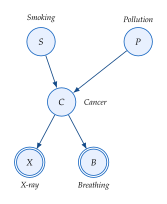
The factorisation implied by Figure fig:medical:bn is: (Factor) $\begin{matrix} P (S, P, C, X, B) = P (S) P (P) P (C | S, P) P (X | C) P (B | C) . \end{matrix}$

Example 3 (Counting Parameters).

If all five variables are binary, the full joint needs $2^{5} - 1 = 31$ free parameters. The Bayesian network needs: $\underset{P (S)}{\underset{⏟}{1}} + \underset{P (P)}{\underset{⏟}{1}} + \underset{P (C | S, P)}{\underset{⏟}{4}} + \underset{P (X | C)}{\underset{⏟}{2}} + \underset{P (B | C)}{\underset{⏟}{2}} = 10 parameters.$ This is a $3 \times$ reduction for just 5 variables; the savings grow exponentially with the number of variables.

Plate Notation

When a graphical model contains repeated structure ( $N$ data points drawn independently from the same model) drawing $N$ copies of the subgraph is impractical. Plate notation uses a rectangle (“plate”) to indicate replication.

Plate notation for a Gaussian mixture model. The outer plate indicates

N

i.i.d. data points; the inner plate indicates

K

mixture components. Shaded nodes are observed.

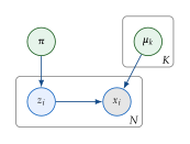
Remark 1 (Reading Plate Diagrams).

Shaded nodes are observed; unshaded are latent.
Nodes outside a plate are shared across all copies.
Nodes inside a plate are replicated.
Arrows crossing a plate boundary mean every copy of the inner node receives the same parent.

The plate diagram in Figure fig:plate:gmm encodes: $P (𝒙, 𝒛, 𝝅, 𝝁) = P (𝝅) \prod_{k = 1}^{K} P (𝝁_{k}) \prod_{i = 1}^{N} P (z_{i} | 𝝅) P (x_{i} | z_{i}, 𝝁)$ .

Conditional Independence and d-Separation

The power of a graphical model lies not just in the factorisation it implies, but in the conditional independence (CI) statements we can read directly from the graph. The criterion for reading CI from a DAG is called d-separation.

Three Canonical Structures

Every path in a DAG is built from three atomic motifs. Understanding these three cases is the key to understanding d-separation.

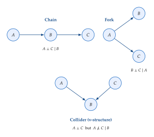
The three canonical structures in a DAG. In chains and forks, conditioning on the middle node blocks the path. In a collider, the path is blocked by default but opens when we condition on the middle node (or any of its descendants).

Definition 2 (The Three Canonical Structures).

Let $A$ , $B$ , $C$ be three nodes connected by a path in a DAG.

Chain: $A \to B \to C$ . Conditioning on $B$ blocks the flow of information from $A$ to $C$ : $A ⟂ C | B$ .
Fork: $A \leftarrow B \to C$ (equivalently $B \to A$ and $B \to C$ ). $B$ is a common cause. Conditioning on $B$ blocks the path: $A ⟂ C | B$ .
Collider (v-structure): $A \to B \leftarrow C$ . The path is blocked by default: $A ⟂ C$ . Conditioning on $B$ (or any descendant of $B$ ) opens the path: $A ⟂̸ C | B$ .

Example 4 (Explaining Away).

Suppose $A$ = “earthquake” and $C$ = “burglar alarm malfunction”, both of which can cause $B$ = “alarm sounds”. Marginally, $A$ and $C$ are independent (earthquakes have nothing to do with alarm malfunctions). But if you observe that the alarm sounded ( $B$ ), learning that an earthquake occurred ( $A$ ) makes a malfunction ( $C$ ) less likely, since the earthquake already “explains away” the alarm. This is the collider effect: conditioning on $B$ induces a dependence between its parents.

The d-Separation Criterion

Definition 3 (d-Separation).

Let $𝒢$ be a DAG and let $𝐀$ , $𝐁$ , $𝐂$ be disjoint sets of nodes. A path between a node in $𝐀$ and a node in $𝐁$ is blocked by $𝐂$ if it contains a node $Z$ such that either:

$Z \in 𝐂$ and $Z$ is not a collider on the path (chain or fork), or
$Z$ is a collider on the path and neither $Z$ nor any descendant of $Z$ is in $𝐂$ .

$𝐀$ and $𝐁$ are d-separated given $𝐂$ , written $𝐀 ⟂_{𝒢} 𝐁 | 𝐂$ , if every path between $𝐀$ and $𝐁$ is blocked by $𝐂$ .

Theorem 1 (Soundness and Completeness of d-Separation).

Let $P$ be a distribution that factorises according to DAG $𝒢$ . Then for all disjoint sets $𝐀$ , $𝐁$ , $𝐂$ : $𝐀 ⟂_{𝒢} 𝐁 | 𝐂 ⟹ 𝐀 ⟂_{P} 𝐁 | 𝐂 .$ Moreover, if $P$ is a faithful distribution for $𝒢$ (i.e. the only CIs in $P$ are those implied by $𝒢$ ), then the converse also holds.

Example 5 (Applying d-Separation).

In the medical diagnosis network (Figure fig:medical:bn):

Is $S ⟂ P$ ? Yes, there is no path between $S$ and $P$ that does not go through collider $C$ , so the path is blocked. Smoking and pollution are a priori independent.
Is $S ⟂ P | C$ ? No, $C$ is a collider between $S$ and $P$ , and conditioning on it opens the path. If you know someone has cancer, learning they smoke makes pollution a less likely cause (explaining away).
Is $X ⟂ B | C$ ? Yes, both paths from $X$ to $B$ go through $C$ , and conditioning on $C$ blocks the chains $X \leftarrow C \to B$ . Once we know the cancer status, the X-ray result tells us nothing extra about breathing difficulty.

Markov Blanket

Definition 4 (Markov Blanket).

The Markov blanket of a node $X_{i}$ in a Bayesian network is the set: $MB (X_{i}) = Pa (X_{i}) \cup Ch (X_{i}) \cup CoPa (X_{i}),$ where $Ch (X_{i})$ are the children of $X_{i}$ and $CoPa (X_{i})$ are the other parents of $X_{i}$ 's children.

Proposition 1 (Markov Blanket Property).

A node $X_{i}$ is conditionally independent of all other variables in the network given its Markov blanket: $X_{i} ⟂ (𝒱 ∖ {X_{i}} ∖ MB (X_{i})) | MB (X_{i}) .$

Proof.

By the factorisation , $P (X_{i} | 𝒱 ∖ {X_{i}})$ depends only on the factors that involve $X_{i}$ : its own CPD $P (X_{i} | Pa (X_{i}))$ and the CPDs of its children $P (X_{c} | Pa (X_{c}))$ for $X_{c} \in Ch (X_{i})$ . These factors involve exactly the parents, children, and co-parents of $X_{i}$ .

∎

Insight.

The Markov blanket defines the minimal sufficient context for a variable; everything outside the blanket is irrelevant once the blanket is known. In Gibbs sampling (Chapter 6), we sample each variable from its conditional given its Markov blanket, which is efficient because the blanket is typically small relative to the full network.

Undirected Graphical Models: Markov Random Fields

Not all dependencies are naturally directional. In an image, nearby pixels influence each other symmetrically. In a protein, amino acids interact via symmetric physical forces. Undirected graphical models capture such symmetric relationships.

Definition 5 (Markov Random Field).

A Markov random field (MRF), also called an undirected graphical model, consists of an undirected graph $𝒢 = (𝒱, ℰ)$ and a set of non-negative potential functions ${ψ_{c}}_{c \in 𝒞}$ , one per maximal clique $c$ of $𝒢$ . The joint distribution is (MRF) $\begin{matrix} P (𝒙) = \frac{1}{Z} \prod_{c \in 𝒞} ψ_{c} (𝒙_{c}), Z = \sum_{𝒙} \prod_{c \in 𝒞} ψ_{c} (𝒙_{c}), \end{matrix}$ where $Z$ is the partition function ensuring normalisation, and $𝒙_{c}$ denotes the variables in clique $c$ .

Remark 2 (Potentials Are Not Probabilities).

Unlike CPDs in Bayesian networks, potential functions $ψ_{c} (𝒙_{c})$ are not probability distributions; they are arbitrary non-negative functions. This extra flexibility comes at a cost: computing the partition function $Z$ is generally intractable (it sums over all $| 𝒳 |^{n}$ configurations).

Example 6 (The Ising Model).

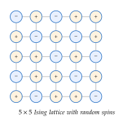
The Ising model, introduced by physicist Ernst Ising in 1925 [5], is perhaps the most famous MRF. Each node $i$ on a lattice takes a spin $x_{i} \in {- 1, + 1}$ , and neighbouring spins prefer to align: (Ising) $\begin{matrix} P (𝒙) = \frac{1}{Z} \exp (β \sum_{(i, j) \in ℰ} x_{i} x_{j} + h \sum_{i} x_{i}), \end{matrix}$ where $β > 0$ controls the coupling strength and $h$ is an external field. The pairwise potential is $ψ_{i j} (x_{i}, x_{j}) = \exp (β x_{i} x_{j})$ , which is large when $x_{i} = x_{j}$ (spins aligned) and small when $x_{i} \neq x_{j}$ .

At high temperature ( $β \to 0$ ) the spins are nearly independent; at low temperature ( $β \to \infty$ ) they strongly align. The transition between these regimes is a phase transition, a phenomenon of deep importance in both physics and generative modelling (where it manifests as “mode collapse” or sharp transitions in sample quality).

5 \times 5

Ising model on a grid. Orange (

+

) and blue (

-

) nodes represent spin up and spin down. Each edge connects neighbouring spins with a pairwise potential favouring alignment.

The Hammersley–Clifford Theorem

The following theorem provides the theoretical foundation for MRFs, establishing the equivalence between the graph structure and the factorisation.

Theorem 2 (Hammersley–Clifford).

Let $P$ be a strictly positive distribution over $𝒱$ and let $𝒢$ be an undirected graph. Then $P$ satisfies the pairwise Markov property with respect to $𝒢$ : $X_{i} ⟂ X_{j} | 𝒱 ∖ {X_{i}, X_{j}} whenever (i, j) \notin ℰ,$ if and only if $P$ factorises over the cliques of $𝒢$ as in .

Remark 3 (Energy-Based Interpretation).

Writing $ψ_{c} (𝒙_{c}) = \exp (- E_{c} (𝒙_{c}))$ , the MRF becomes $P (𝒙) = \frac{1}{Z} \exp (- \sum_{c \in 𝒞} E_{c} (𝒙_{c})) = \frac{1}{Z} \exp (- E (𝒙)),$ a Gibbs distribution with energy $E (𝒙)$ . Low-energy configurations have high probability. This is exactly the framework of energy-based models (EBMs), a family of generative models where a neural network parameterises the energy function $E_{θ} (𝒙)$ .

Directed vs. Undirected Models

Property	Bayesian Network (Directed)	MRF (Undirected)
Edge meaning	Causal / generative direction	Symmetric association
Factorisation	$\prod_{i} P (X_{i} \| Pa (X_{i}))$	$\frac{1}{Z} \prod_{c} ψ_{c} (𝒙_{c})$
Normalisation	Automatic (CPDs normalise)	Requires partition function $Z$
CI criterion	d-separation	Graph separation
Typical use	Causal modelling, VAEs, autoregressive	Physics, images, EBMs

Comparison of directed and undirected graphical models.

Factor Graphs

Both directed and undirected models can be represented in a unified framework called a factor graph.

Definition 6 (Factor Graph).

A factor graph is a bipartite graph $𝒢 = (𝒱, ℱ, ℰ)$ with:

Variable nodes $𝒱 = {X_{1}, \dots, X_{n}}$ (drawn as circles).
Factor nodes $ℱ = {f_{1}, \dots, f_{m}}$ (drawn as small squares).
An edge between $X_{i}$ and $f_{a}$ iff $X_{i}$ appears in factor $f_{a}$ .

The joint distribution is (Graph) $\begin{matrix} P (𝒙) = \frac{1}{Z} \prod_{a = 1}^{m} f_{a} (𝒙_{𝒩 (a)}), \end{matrix}$ where $𝒩 (a)$ is the set of variable nodes neighbouring factor $f_{a}$ .

Example 7 (Converting a Bayesian Network to a Factor Graph).

Given the medical diagnosis Bayesian network $P (S, P, C, X, B) = P (S) P (P) P (C | S, P) P (X | C) P (B | C)$ , we create one factor node for each CPD: $f_{1} = P (S)$ , $f_{2} = P (P)$ , $f_{3} = P (C | S, P)$ , $f_{4} = P (X | C)$ , $f_{5} = P (B | C)$ . Each factor connects to its argument variables. The partition function $Z = 1$ since the factors are proper conditional distributions.

Insight.

Factor graphs are the natural framework for message-passing algorithms. On a tree-structured factor graph, the sum-product algorithm (belief propagation) computes exact marginals in time linear in the number of nodes. This is the algorithmic engine behind many inference procedures in generative models.

Inference in Graphical Models

Given a graphical model, inference means computing quantities of interest from the joint distribution, typically marginal probabilities or the most likely configuration.

Definition 7 (Marginal and MAP Inference).

Given a joint $P (𝒙)$ and a partition of variables into query $𝐐$ and evidence $𝐄 = 𝒆$ :

Marginal inference: compute $P (𝐐 | 𝐄 = 𝒆) = \sum_{𝐑} P (𝐐, 𝐑 | 𝒆)$ , where $𝐑$ are the remaining (hidden) variables.
MAP inference: find $\hat{𝒙} = {arg max}_{𝐐} P (𝐐 | 𝐄 = 𝒆)$ .

Variable Elimination

The brute-force approach sums over all configurations, exponential in the number of variables. Variable elimination exploits the factorisation to sum out variables one at a time, dramatically reducing the cost.

Algorithm 1 (Variable Elimination).

Input: Factors ${f_{1}, \dots, f_{m}}$ , query variable $Q$ , elimination ordering $(X_{e_{1}}, X_{e_{2}}, \dots)$ . Output: Marginal $P (Q)$ (unnormalised).

for each variable $X_{e_{i}}$ in the elimination ordering:

Collect all factors $𝒮_{i}$ that mention $X_{e_{i}}$ .
Compute the product $τ_{i} (\cdot) = \sum_{X_{e_{i}}} \prod_{f \in 𝒮_{i}} f (\cdot)$ .
Replace $𝒮_{i}$ by the new factor $τ_{i}$ in the factor set.

return the product of all remaining factors (which involve only $Q$ ).

Example 8 (Variable Elimination Walkthrough).

Consider the chain $A \to B \to C \to D$ with $P (A, B, C, D) = P (A) P (B | A) P (C | B) P (D | C)$ . To compute $P (D)$ , we eliminate $A$ , $B$ , $C$ in order: $\begin{matrix} Eliminate A & : τ_{1} (B) = \sum_{A} P (A) P (B | A), \\ Eliminate B & : τ_{2} (C) = \sum_{B} τ_{1} (B) P (C | B), \\ Eliminate C & : P (D) = \sum_{C} τ_{2} (C) P (D | C) . \end{matrix}$ Each step sums over one variable in a small factor, avoiding exponential blowup. If each variable takes $k$ values, the cost is $O (n k^{2})$ instead of $O (k^{n})$ .

Caution.

The cost of variable elimination depends critically on the elimination ordering. A bad ordering can create intermediate factors that are exponentially large. Finding the optimal ordering is NP-hard in general. In practice, heuristics like minimum degree or minimum fill work well for sparse graphs.

Belief Propagation

On tree-structured graphs, variable elimination can be organised as a message-passing algorithm: each node sends a “message,” a function summarising its local information, to its neighbours.

Definition 8 (Sum-Product Messages on a Factor Tree).

On a factor graph that is a tree, the message from variable node $X_{i}$ to factor node $f_{a}$ is: (Factor) $\begin{matrix} m_{X_{i} \to f_{a}} (x_{i}) = \prod_{f_{b} \in 𝒩 (X_{i}) ∖ {f_{a}}} m_{f_{b} \to X_{i}} (x_{i}), \end{matrix}$ and the message from factor $f_{a}$ to variable $X_{i}$ is: (VAR) $\begin{matrix} m_{f_{a} \to X_{i}} (x_{i}) = \sum_{𝒙_{𝒩 (a) ∖ {i}}} f_{a} (𝒙_{𝒩 (a)}) \prod_{X_{j} \in 𝒩 (a) ∖ {X_{i}}} m_{X_{j} \to f_{a}} (x_{j}) . \end{matrix}$ The marginal of $X_{i}$ is proportional to the product of all incoming messages: $P (x_{i}) \propto \prod_{f_{a} \in 𝒩 (X_{i})} m_{f_{a} \to X_{i}} (x_{i})$ .

Theorem 3 (Exactness on Trees).

On a tree-structured factor graph, belief propagation computes exact marginals for every variable in $O (n k^{w})$ time, where $n$ is the number of variables, $k$ is the domain size, and $w$ is the maximum factor size.

Remark 4 (Loopy Belief Propagation).

On graphs with cycles, belief propagation can still be run by iterating messages until convergence, a heuristic known as loopy belief propagation. It has no convergence guarantees in general, but works surprisingly well in practice and forms the basis of algorithms for error-correcting codes (turbo codes, LDPC codes) and computer vision [6].

When Exact Inference Is Intractable

Key Idea.

For general graphs, exact inference is NP-hard. This fundamental intractability is what motivates the two major families of approximate inference:

Variational inference: approximate the posterior with a tractable family, optimising a bound (Chapter 8).
Sampling methods (MCMC): draw correlated samples from the posterior, with convergence guarantees in the limit.

Understanding why exact inference is hard provides the motivation for the variational methods that power modern generative models like VAEs.

Learning in Graphical Models

Learning a graphical model from data involves estimating the parameters $Θ$ (and potentially the structure $𝒢$ ) given a dataset $𝒟 = {𝒙^{(1)}, \dots, 𝒙^{(N)}}$ .

Maximum Likelihood with Complete Data

When all variables are observed (“complete data”), MLE in a Bayesian network decomposes into independent subproblems.

Proposition 2 (MLE Decomposes over CPDs).

For a Bayesian network with complete data, the log-likelihood is $ℓ (Θ) = \sum_{i = 1}^{n} \sum_{j = 1}^{N} \log P_{θ_{i}} (x_{i}^{(j)} | Pa {(x_{i})}^{(j)}),$ which decomposes into $n$ independent terms, one per node. Each CPD can be estimated separately.

Example 9 (MLE for a Discrete CPD).

In the medical diagnosis network, suppose we observe $N$ data points and want to estimate $P (C = 1 | S = s, P = p)$ for each configuration of parents. The MLE is simply the empirical frequency: $\hat{P} (C = 1 | S = s, P = p) = \frac{# {i : C^{(i)} = 1, S^{(i)} = s, P^{(i)} = p}}{# {i : S^{(i)} = s, P^{(i)} = p}} .$ This is just counting, no optimisation needed!

Learning with Latent Variables: The EM Algorithm

When some variables are latent (unobserved), the log-likelihood no longer decomposes, and MLE becomes much harder.

Definition 9 (The EM Algorithm).

Given observed data $𝒙$ and latent variables $𝒛$ , the Expectation-Maximisation (EM) algorithm iterates:

E-step: Compute the posterior over latent variables using current parameters: $q (𝒛) = P (𝒛 | 𝒙; θ^{(t)}) .$
M-step: Maximise the expected complete-data log-likelihood: $θ^{(t + 1)} = {arg max}_{θ} 𝔼_{q (𝒛)} [\log P (𝒙, 𝒛; θ)] .$

Proposition 3 (EM Monotonically Increases Likelihood).

Each iteration of EM is guaranteed to increase (or leave unchanged) the observed-data log-likelihood: $\log P (𝒙; θ^{(t + 1)}) \geq \log P (𝒙; θ^{(t)})$ .

Proof sketch.

By Jensen's inequality, the E-step constructs a lower bound on $\log P (𝒙; θ)$ that is tight at $θ^{(t)}$ . The M-step maximises this bound, which can only increase the objective. See Chapter 8 for the detailed connection to variational inference.

∎

Insight.

The EM algorithm is the bridge between graphical models and generative modelling:

For Gaussian mixture models (Chapter 7), EM alternates between computing cluster responsibilities (E-step) and updating means/covariances (M-step).
For VAEs, the E-step is intractable, so we replace it with an amortised encoder $q_{ϕ} (𝒛 | 𝒙)$ , the “variational” in VAE.
For diffusion models, the forward process defines the latent structure, and training optimises a variational bound similar to the EM objective.

PGMs as the Language of Generative Models

Every generative model we will study in this book has a natural PGM representation. Recognising this structure helps us understand what independence assumptions each model makes, what inference challenges it faces, and why particular training objectives are used.

PGM representations of three major generative model families. Left: A VAE with latent

𝒛

and observed

𝒙

; the dashed red arrow is the inference network

q_{ϕ} (𝒛 | 𝒙)

. Centre: An autoregressive model as a fully-connected DAG (each

x_{t}

depends on all predecessors). Right: A diffusion model as a Markov chain; grey arrows are the fixed forward process

q

, red arrows are the learned reverse

p_{θ}

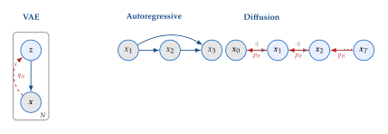
Model Family	Graph Type	Key Challenge	Solution Strategy
Autoregressive	Directed (chain)	Sequential generation	Parallel training, caching
VAE	Directed (latent)	Intractable posterior	Amortised variational inference
GAN	Implicit (no explicit $P$ )	Adversarial training	Discriminator as density ratio
Normalising Flow	Directed (bijective)	Jacobian cost	Triangular / coupling layers
Diffusion	Directed (Markov chain)	Long chain	Score matching, DDPM bound
Energy-Based	Undirected	Partition function $Z$	Contrastive divergence, score matching

Generative model families viewed through the PGM lens.

Remark 5 (The Implicit Model Exception).

GANs are sometimes called implicit generative models because they define a sampling procedure $𝒛 \mapsto G_{θ} (𝒛)$ without specifying $P (𝒙)$ explicitly. They do not naturally fit the PGM framework, since there is no tractable density. This is both a strength (no normalisation constant) and a weakness (no likelihood for evaluation).

Independence Maps and Perfect Maps

A natural question arises: can we always find a graph that exactly captures all the conditional independences in a given distribution?

Definition 10 (I-map, D-map, Perfect Map).

Let $P$ be a distribution and $𝒢$ a graph.

$𝒢$ is an independence map (I-map) for $P$ if every CI implied by $𝒢$ holds in $P$ . (The graph may “miss” some independences.)
$𝒢$ is a dependence map (D-map) for $P$ if every CI in $P$ is captured by $𝒢$ . (The graph may assert too many independences.)
$𝒢$ is a perfect map for $P$ if it is both an I-map and a D-map, meaning the graph captures exactly the CIs in $P$ .

Example 10 (No Perfect Directed Map).

Consider four binary variables $A, B, C, D$ with the CI structure: $A ⟂ C | {B, D}$ and $B ⟂ D | {A, C}$ , but no other CIs. It can be shown that no DAG is a perfect map for this distribution, but an undirected graph (a 4-cycle $A - B - C - D - A$ ) is. This illustrates why we need both directed and undirected models.

Caution.

The existence of a perfect map is a strong assumption. In practice, we choose a graph family (directed or undirected) that captures the most important dependencies, accepting that some independences may be missed or incorrectly asserted. The choice of graph family is a modelling decision with practical consequences for inference and learning.

Chapter Summary

This chapter introduced the language of probabilistic graphical models, the formal backbone of generative modelling.

Bayesian networks (directed models) represent joint distributions via CPDs and DAGs; d-separation reads off conditional independences.
Markov random fields (undirected models) use clique potentials and partition functions; the Hammersley–Clifford theorem connects graph structure to factorisation.
Factor graphs unify both representations and enable message-passing inference.
Inference (variable elimination, belief propagation) is exact on trees but NP-hard in general, motivating the variational methods of Chapter 8.
Learning with complete data is straightforward (MLE decomposes); with latent variables, EM provides an iterative solution.
Every major generative model family has a natural PGM interpretation, making graphical models the lingua franca of the field.

In the next chapter, we study Gaussian mixture models, the simplest and most instructive latent-variable model, where the EM algorithm can be derived in closed form.

Exercises

Exercise 1 (Factorisation and Parameter Counting).

Consider a DAG with four binary random variables $A$ , $B$ , $C$ , $D$ and edges $A \to B$ , $A \to C$ , $B \to D$ , $C \to D$ .

(a)
Write down the factorisation of $P (A, B, C, D)$ .
(b)
How many free parameters does this model need?
(c)
Compare to the $2^{4} - 1 = 15$ parameters for the full joint.

Exercise 2 (Collider and Explaining Away).

Let $X$ , $Y$ , $Z$ be random variables in a DAG with edges $X \to Z$ and $Y \to Z$ (a v-structure).

(a)
Show that $X ⟂ Y$ marginally.
(b)
Show that $X ⟂̸ Y | Z$ .
(c)
Explain intuitively why observing $Z$ creates a dependence (the “explaining away” effect).

Exercise 3 (d-Separation Practice).

Consider a DAG with nodes ${A, B, C, D, E}$ and edges $A \to C$ , $B \to C$ , $C \to D$ , $C \to E$ . Determine which hold:

(a)
$A ⟂ B$
(b)
$A ⟂ B | C$
(c)
$D ⟂ E | C$
(d)
$A ⟂ E | D$
(e)
$D ⟂ B | {A, C}$

Justify each answer by identifying paths and their blocking status.

Exercise 4 (Markov Blanket Computation).

For the graph with edges $A \to B$ , $A \to C$ , $B \to D$ , $C \to D$ , $D \to E$ :

(a)
Prove that $X$ is conditionally independent of all other variables given its Markov blanket.
(b)
Compute $MB (X)$ for every node $X$ .

Exercise 5 (Constructing a Medical Bayesian Network).

Variables: Smoking ( $S$ ), Pollution ( $P$ ), Cancer ( $C$ ), X-ray ( $X$ ), Breathing difficulty ( $B$ ). Domain knowledge:

$S$ and $P$ are independent risk factors.
$C$ depends on both $S$ and $P$ .
$X$ and $B$ each depend on $C$ .

(a)
Draw the Bayesian network.
(b)
Write the factorisation of the joint.
(c)
Count parameters (binary variables) and compare to the full joint.
(d)
Does $X ⟂ B | C$ hold? Interpret medically.

Exercise 6 (Hidden Markov Model).

An HMM has latent states $Z_{1}, \dots, Z_{T}$ and observations $X_{1}, \dots, X_{T}$ , where $Z_{t}$ depends only on $Z_{t - 1}$ and $X_{t}$ depends only on $Z_{t}$ .

(a)
Draw the DAG and write the joint factorisation.
(b)
Show that $X_{i} ⟂ X_{j} | Z_{i}, Z_{j}$ for $i \neq j$ .
(c)
Show that $X_{1} ⟂̸ X_{T}$ marginally when $T \geq 2$ .
(d)
What is the Markov blanket of $Z_{t}$ (for $1 < t < T$ )?

Exercise 7 (GMM Plate Diagram).

A Gaussian mixture model has $N$ data points, $K$ components, mixing weights $𝝅$ , means $𝝁_{k}$ , and covariances $𝚺_{k}$ .

(a)
Draw the plate diagram.
(b)
Identify observed, latent, and parameter nodes.
(c)
Write the complete joint $P (𝒙, 𝒛, 𝝅, 𝝁, 𝚺)$ with appropriate priors.

Exercise 8 (Ising Model Computation).

Consider a $2 \times 2$ Ising model (4 spins on a grid) with $β = 1$ and $h = 0$ .

(a)
List all $2^{4} = 16$ configurations and compute the unnormalised probability for each.
(b)
Compute the partition function $Z$ .
(c)
What is the probability that all four spins are aligned ( $+ + + +$ or $- - - -$ )?
(d)
What is the marginal probability $P (x_{1} = + 1)$ ?

Exercise 9 (Variable Elimination Ordering).

Consider a “diamond” DAG: $A \to B$ , $A \to C$ , $B \to D$ , $C \to D$ , all binary. You want to compute $P (D)$ .

(a)
Perform variable elimination with ordering $(C, B, A)$ . What is the size of the largest intermediate factor?
(b)
Repeat with ordering $(A, B, C)$ .
(c)
Which ordering is more efficient and why?

Exercise 10 (MRF Factorisation).

An undirected graph has nodes ${A, B, C, D}$ and edges $A - B$ , $B - C$ , $C - D$ , $D - A$ (a 4-cycle).

(a)
List the maximal cliques.
(b)
Write the MRF factorisation.
(c)
What conditional independences does this graph encode?
(d)
Can this CI structure be represented by any DAG? (Hint: see Example Example 10.)

Exercise 11 (EM for a Simple Latent Variable Model).

Consider a mixture of two coins: coin 1 has $P (heads) = p_{1}$ and coin 2 has $P (heads) = p_{2}$ , with mixing weight $π$ . You observe $N$ flips but don't know which coin was used for each flip.

(a)
Write the complete-data log-likelihood $\log P (𝒙, 𝒛; π, p_{1}, p_{2})$ .
(b)
Derive the E-step: compute $q (z_{i} = 1) = P (z_{i} = 1 | x_{i}; θ^{(t)})$ .
(c)
Derive the M-step updates for $π$ , $p_{1}$ , $p_{2}$ .
(d)
Implement EM and test on simulated data with $π = 0.3$ , $p_{1} = 0.2$ , $p_{2} = 0.8$ , $N = 200$ .

Exercise 12 (Belief Propagation on a Chain).

Consider a 3-node chain: $X_{1} - X_{2} - X_{3}$ with pairwise potentials $ψ_{12} (x_{1}, x_{2})$ and $ψ_{23} (x_{2}, x_{3})$ , and unary potentials $ψ_{i} (x_{i})$ for each node. All variables are binary.

(a)
Write out the messages $m_{X_{1} \to X_{2}}$ , $m_{X_{3} \to X_{2}}$ , and the belief $b (x_{2})$ .
(b)
Verify that $b (x_{2}) \propto P (x_{2})$ (the true marginal).
(c)
If $ψ_{12} = ψ_{23} = (\begin{matrix} 5 & 1 \\ 1 & 5 \end{matrix})$ and $ψ_{i} \equiv 1$ , compute $P (X_{2} = 0)$ and $P (X_{2} = 1)$ .

Exercise 13 (VAE as a Graphical Model).

A variational autoencoder has the generative model $𝒛 \sim Normal (0, I)$ , $𝒙 | 𝒛 \sim Normal (μ_{θ} (𝒛), σ_{θ}^{2} (𝒛) I)$ .

(a)
Draw the directed graphical model (with plate notation for $N$ data points).
(b)
Why is the posterior $P (𝒛 | 𝒙)$ intractable?
(c)
The encoder $q_{ϕ} (𝒛 | 𝒙)$ is not part of the generative model. Where does it appear in the PGM, and what role does it play?
(d)
Connect this to the EM algorithm: what plays the role of the E-step? The M-step?

Exercise 14 (Directed vs. Undirected Expressiveness).

(a)
Give an example of a CI structure that can be represented by a DAG but not by any undirected graph. (Hint: consider a v-structure.)
(b)
Give an example that can be represented by an undirected graph but not by any DAG. (Hint: consider a 4-cycle.)
(c)
What does this tell us about the relative expressiveness of directed and undirected models?

Notes

The name is historical; a Bayesian network does not require Bayesian (as opposed to frequentist) statistical methods.

References

Correlation and Causation

Sewall Wright

Journal of Agricultural Research, vol. 20, no. 7, pp. 557-585 · 1921

BibTeX

@article{wright1921correlation,
  title={Correlation and Causation},
  author={Wright, Sewall},
  journal={Journal of Agricultural Research},
  volume={20},
  number={7},
  pages={557--585},
  year={1921}
}

Journal article

Probabilistic Reasoning in Intelligent Systems: Networks of Plausible Inference

Judea Pearl

Morgan Kaufmann · 1988

BibTeX

@book{pearl1988probabilistic,
  title={Probabilistic Reasoning in Intelligent Systems: Networks of Plausible Inference},
  author={Pearl, Judea},
  publisher={Morgan Kaufmann},
  year={1988}
}

Book

Markov Fields on Finite Graphs and Lattices

John M Hammersley, Peter Clifford

1971

BibTeX

@unpublished{hammersley1971markov,
  title={Markov Fields on Finite Graphs and Lattices},
  author={Hammersley, John M and Clifford, Peter},
  year={1971},
  note={Unpublished manuscript}
}

Reference

Probabilistic Graphical Models: Principles and Techniques

Daphne Koller, Nir Friedman

MIT Press · 2009

BibTeX

@book{koller2009probabilistic,
  title={Probabilistic Graphical Models: Principles and Techniques},
  author={Koller, Daphne and Friedman, Nir},
  publisher={MIT Press},
  address={Cambridge, MA},
  year={2009}
}

Book

Beitrag zur Theorie des Ferromagnetismus

Ernst Ising

Zeitschrift fur Physik, vol. 31, no. 1, pp. 253-258 · 1925

BibTeX

@article{ising1925beitrag,
  title={{Beitrag zur Theorie des Ferromagnetismus}},
  author={Ising, Ernst},
  journal={Zeitschrift f{\"u}r Physik},
  volume={31},
  number={1},
  pages={253--258},
  year={1925}
}

Journal article

Understanding Belief Propagation and Its Generalizations

Jonathan S Yedidia, William T Freeman, Yair Weiss

Exploring Artificial Intelligence in the New Millennium, vol. 8, pp. 236-239 · 2003

BibTeX

@article{yedidia2003understanding,
  title={Understanding Belief Propagation and Its Generalizations},
  author={Yedidia, Jonathan S and Freeman, William T and Weiss, Yair},
  journal={Exploring Artificial Intelligence in the New Millennium},
  volume={8},
  pages={236--239},
  year={2003}
}

Journal article

← 5 Deep Learning Building Blocks 7 Gaussian Mixture Models →