5 Deep Learning Building Blocks
In Chapter 3 we formalised the generative modelling problem as finding a map such that the push-forward approximates . But what is ? In virtually every modern generative model, it is a deep neural network, a composition of simple, parameterised, differentiable functions that can approximate extraordinarily complex mappings.
This chapter introduces the neural network building blocks that the rest of the book relies on: feedforward layers, activation functions, convolutional and transposed-convolutional layers, residual connections, normalisation layers, and the Transformer's attention mechanism. For each building block, we give the mathematical definition, state its key properties, and explain why it appears in specific generative model architectures.
Historical Note.
The idea of modelling computation with networks of artificial neurons dates to McCulloch and Pitts (1943) [1]. Rosenblatt's perceptron (1958) [2] could learn from data, but Minsky and Papert (1969) [3] showed it could not solve non-linearly-separable problems like XOR, triggering the first “AI winter.” The field revived in the 1980s with backpropagation [4] and again in the 2010s when GPUs, large datasets, and deeper architectures led to breakthroughs in vision [5] and language [6]. Today, deep networks with billions of parameters are the engine behind every generative model studied in this book.
Feedforward Neural Networks
Definition 1 (Feedforward Neural Network).
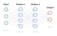
An -layer feedforward neural network (also called a multilayer perceptron, MLP) computes a function by alternating affine transformations and element-wise nonlinearities: (FFN) where is the input, is a weight matrix, is a bias vector, and is a nonlinear activation function. The output is (or if the last layer is linear). The collection of all weights and biases is .
Activation Functions
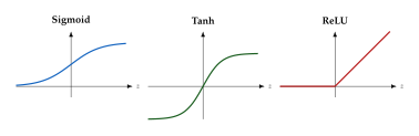
The activation function introduces nonlinearity. Without it, the composition of affine layers would itself be affine, and the network could only represent linear functions.
Definition 2 (Common Activation Functions).
(Sigmoid) where is the standard Gaussian CDF.
Remark 1 (Which Activation Where?).
ReLU and Leaky ReLU are standard in CNNs and GAN discriminators [7].
GELU and SiLU/Swish are used in Transformers (GPT, diffusion U-Nets) due to smoother gradients.
Sigmoid appears as the output activation for GAN discriminators (outputting a probability) and in LSTM gates.
Tanh is often used in the final layer of image generators (mapping to pixel range).
The Universal Approximation Theorem
Why are neural networks so effective as the generator ? The following foundational result answers this question.
Theorem 1 (Universal Approximation - Cybenko 1989, Hornik 1991).
Let be any continuous, non-constant activation function. For any continuous function and any , there exists a single-hidden-layer network with sufficiently large such that .
Caution.
The universal approximation theorem guarantees existence but says nothing about how to find the weights, nor about the required width (which can be exponential in ). In practice, depth is far more efficient than width: deep networks can represent functions with exponentially fewer parameters than shallow ones. This is why generative models use networks with dozens to hundreds of layers, not single-layer networks with billions of neurons.
Insight.
The universal approximation theorem tells us that a neural network is, in principle, flexible enough to represent any continuous push-forward map, from a Gaussian latent space to the space of natural images. The practical challenge is finding good weights via training, which is the subject of the next section.
Training Neural Networks
Loss Functions and Gradient Descent
Training a neural network means finding parameters that minimise a loss function that measures discrepancy between the network's predictions and the training data: (LOSS) where is a per-sample loss (e.g. mean squared error, cross-entropy).
Definition 3 (Gradient Descent).
Gradient descent iteratively updates parameters in the direction of steepest decrease of : (GD) where is the learning rate.
Definition 4 (Stochastic Gradient Descent (SGD)).
When the dataset is large, computing the full gradient is expensive. SGD approximates it using a random mini-batch of size : (SGD) The mini-batch gradient is an unbiased estimate of the full gradient, with variance proportional to .
Remark 2 (Adam and Modern Optimisers).
In practice, most generative models use Adam (Adaptive Moment Estimation), which maintains running averages of both the gradient and its square, adapting the learning rate per parameter. Variants like AdamW (with weight decay) are standard for Transformers, while SGD with momentum remains popular for CNNs.
Backpropagation
Computing for a deep network uses the chain rule of calculus, applied layer by layer from the output back to the input. This algorithm, called backpropagation [4], is the workhorse of deep learning.
Algorithm 1 (Backpropagation (Sketch)).
Key Idea.
Backpropagation computes the gradient of a loss with respect to all parameters in time, regardless of how many parameters there are. This efficiency is what makes training networks with millions (or billions) of parameters feasible. It is implemented automatically by frameworks like PyTorch via automatic differentiation.
Normalisation Layers
Deep networks are prone to “internal covariate shift,” where the distribution of each layer's inputs shifts as preceding layers update. Normalisation layers stabilise training by re-centring and re-scaling activations.
Definition 5 (Batch Normalisation).
Given a mini-batch of activations at a particular layer, batch normalisation (BN) [8] computes (Batchnorm) where and are the mean and variance over the batch, and are learnable parameters, and is a small constant for numerical stability. BN normalises across the batch dimension.
Definition 6 (Layer Normalisation).
Layer normalisation (LN) [9] normalises across the feature dimension for each sample independently: (Layernorm) where and are per-sample statistics (with features).
Remark 3 (Which Normalisation Where?).
Batch normalisation: default in CNN-based discriminators and early GAN generators [7].
Layer normalisation: standard in Transformers [6] and diffusion-model U-Nets, because it does not depend on batch size and works with variable-length sequences.
Group normalisation and instance normalisation: used in style transfer and some GAN generators (e.g. StyleGAN [10]).
Convolutional Neural Networks
Images have spatial structure: nearby pixels are correlated, and patterns (edges, textures) can appear anywhere in the image. Convolutional neural networks (CNNs) [26] exploit this structure by replacing full matrix multiplications with local, weight-shared convolution operations.
Definition 7 (2D Convolution Layer).
Given an input feature map and a bank of kernels , the output of a 2D convolution is (Conv2d) where is the stride and is a bias.
Example 1 (Convolution Arithmetic).
A convolution with stride 1 and “same” padding applied to a image with 3 input channels and 64 output channels has parameters, far fewer than a fully connected layer (), yet it captures all local patterns.
Insight.
CNNs are the backbone of image-based generative models:
GAN discriminators are typically deep CNNs that progressively downsample the image (strided convolutions) to produce a real/fake score [7].
GAN generators use transposed convolutions (Definition 8) to progressively upsample a latent vector into a full-resolution image.
VAE encoders downsample with convolutions; VAE decoders upsample with transposed convolutions.
Diffusion-model denoisers use a U-Net (The U-Net Architecture), which combines downsampling and upsampling paths.
Transposed Convolutions
Generation requires going from a small latent representation to a large output image. Transposed convolutions (sometimes misleadingly called “deconvolutions”) perform learned upsampling.
Definition 8 (Transposed Convolution).
A transposed convolution with kernel , stride , and padding is the adjoint (transpose) of the corresponding forward convolution. Concretely, it inserts zeros between input elements, then applies a standard convolution with kernel . If the forward convolution maps a input to outputs, the transposed convolution maps a smaller input back to .
Remark 4 (Checkerboard Artifacts).
Transposed convolutions are known to produce “checkerboard artifacts,” regular grid patterns visible in generated images, when the kernel size is not divisible by the stride. Alternative upsampling strategies include nearest-neighbour interpolation followed by a regular convolution, which avoids this issue and is used in modern generators like StyleGAN [11].
Pooling
Pooling layers reduce spatial dimensions by summarising local regions. Max pooling takes the maximum value in each window; average pooling takes the mean. In modern generative models, pooling has largely been replaced by strided convolutions (which are learnable), but global average pooling remains common in discriminators.
Residual Networks and Skip Connections
Training very deep networks (50+ layers) is difficult because gradients can vanish or explode as they propagate through many layers. Residual connections (skip connections) [27] solve this by adding the input of a block directly to its output.
Definition 9 (Residual Block).
A residual block computes (Residual) where is a sub-network (typically two convolutional layers with normalisation and activation). The “” is the skip connection.

Key Idea.
Why do residual connections matter for generative models?
They enable very deep generators and discriminators (100+ layers), which have greater representational power.
The identity mapping through the skip connection ensures that the gradient always has a direct path, preventing vanishing gradients.
Residual blocks are the core building block of U-Nets (The U-Net Architecture), used in virtually all diffusion models.
The U-Net Architecture
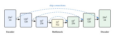
The U-Net, originally proposed for biomedical image segmentation, has become the standard architecture for diffusion-model denoisers (Chapter 16). It consists of:
an encoder (downsampling path) that progressively reduces spatial resolution while increasing channels,
a decoder (upsampling path) that progressively restores resolution, and
long skip connections that concatenate encoder features to the corresponding decoder level, preserving fine-grained spatial information.
Insight.
In diffusion models (Chapter 16), the U-Net takes as input a noisy image and a time step , and predicts the noise that was added. The skip connections are essential: low-level encoder features (edges, textures) help the decoder reconstruct fine details that would otherwise be lost at the bottleneck. The time step is typically injected via learned embeddings added to each residual block, telling the network how much noise to expect.
Sequence Models: From RNNs to Attention
Many data types are sequential: text, audio, time series. Generative models for sequences need architectures that can process variable-length inputs and capture long-range dependencies.
Recurrent Neural Networks
Definition 10 (Recurrent Neural Network).
A recurrent neural network (RNN) processes a sequence by maintaining a hidden state that is updated at each time step: (RNN) where are weight matrices shared across all time steps.
Remark 5 (Vanishing and Exploding Gradients).
Training RNNs via backpropagation through time (BPTT) requires multiplying gradient matrices across time steps. If the spectral radius of is less than 1, gradients vanish exponentially; if greater than 1, they explode. This limits the ability of vanilla RNNs to learn long-range dependencies.
Long Short-Term Memory (LSTM)
Definition 11 (LSTM Cell).
The LSTM introduces a cell state and three gates to control information flow: (LSTM Forget) The forget gate decides what to discard from the cell state; the input gate decides what new information to store.
Remark 6 (From LSTMs to Transformers).
LSTMs dominated sequence modelling from 2014–2017, powering early neural machine translation and text generation. However, their sequential nature (each step depends on the previous) prevents parallelisation across time steps. The Transformer architecture [6] replaced recurrence with attention, enabling massive parallelism and scaling to billions of parameters, a breakthrough that led to GPT, BERT, and modern large language models.
The Transformer
The Transformer [6], introduced in the 2017 paper “Attention Is All You Need,” has become the dominant architecture for both language and vision tasks. Its core innovation is the self-attention mechanism, which allows every position in a sequence to attend to every other position in constant depth.
Scaled Dot-Product Attention
Definition 12 (Scaled Dot-Product Attention).
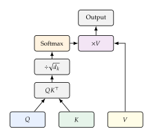
Given queries , keys , and values , the scaled dot-product attention is (Attention) The is applied row-wise, so each row of the output is a weighted combination of the value vectors, where the weights reflect the similarity between the corresponding query and all keys.
Remark 7 (Why Scale by ?).
When is large, the dot products tend to have large magnitude (variance if entries have unit variance), pushing the softmax into saturation where gradients are near zero. Dividing by keeps the variance , ensuring well-behaved gradients throughout training.
Multi-Head Attention
Definition 13 (Multi-Head Attention).
Multi-head attention runs attention functions in parallel, each with its own learned projections: (Multihead) where , , , and are learned projection matrices.
Each head can learn to attend to different aspects of the input (e.g. one head for syntactic relations, another for semantic similarity).
Positional Encoding
Since attention operates on sets (it is permutation-equivariant), we must inject position information explicitly.
Definition 14 (Sinusoidal Positional Encoding).
The original Transformer [6] uses fixed sinusoidal encodings: (Posenc) where is the position index and is the dimension index. These encodings are added to the input embeddings.
Remark 8 (Learnable vs. Sinusoidal Encodings).
Modern models (GPT-2/3, Vision Transformers) often use learned positional embeddings instead. Rotary positional embeddings (RoPE) and ALiBi are recent alternatives that improve length generalisation. We develop RoPE in detail in Rotary Position Embeddings (RoPE) below.
Masked Self-Attention for Autoregressive Generation
In autoregressive generation, position must not attend to any future position (since those tokens have not been generated yet). This is enforced by adding a causal mask: (Causal MASK) The entries become zero after softmax, preventing information leakage from the future.
Insight.
Masked self-attention is the mechanism behind GPT-style autoregressive language models and autoregressive image models (e.g. PixelCNN uses masked convolutions for the same purpose). The chain-rule factorisation from Chapter 3 is implemented by a Transformer decoder with causal masking: each token's prediction depends only on previous tokens.
Cross-Attention for Conditional Generation
In cross-attention, the queries come from one sequence (e.g. the image being generated) while the keys and values come from another (e.g. a text prompt): (Cross ATTN) This is how text-to-image diffusion models (Stable Diffusion, DALL-E) inject the text conditioning signal into the U-Net denoiser.
The Transformer Block
A complete Transformer encoder block combines multi-head self-attention, a feedforward network, residual connections, and layer normalisation:
Algorithm 2 (Transformer Encoder Block).
(self-attention + residual + LN)
(feedforward + residual + LN)
The FFN is typically a two-layer MLP: with GELU or SiLU activation (or SwiGLU, SwiGLU Feedforward Networks).
Remark 9 (Pre-Norm vs. Post-Norm).
The original Transformer applies layer normalisation after the residual addition (“post-norm”). Most modern implementations use “pre-norm” (normalise before attention/FFN), which improves training stability for very deep models.
Rotary Position Embeddings (RoPE)
The sinusoidal positional encoding of Definition 14 is additive: it adds a fixed vector to each token embedding, encoding the absolute position of the token in the sequence. Rotary Position Embeddings (RoPE) [28] take a fundamentally different approach. Instead of adding a position signal to the embeddings, RoPE rotates the query and key vectors in a position-dependent manner before computing the dot-product attention score. The crucial consequence is that the inner product between a rotated query at position and a rotated key at position depends only on their relative distance , not on the absolute positions themselves. This property makes RoPE a natural fit for language modelling and other sequence tasks where relative position carries far more information than absolute position.
Definition 15 (Rotary Position Embedding).
Let be the head dimension (assumed even) and define the frequency schedule (ROPE FREQ) For each position , define the rotation matrix (ROPE) where each block is the standard planar rotation Given an input token at position , the RoPE-augmented query and key are (ROPE QK) where are the usual query and key projection matrices. The attention score between positions and is then .
Note that RoPE modifies only the queries and keys; the value projections and the rest of the Transformer block remain unchanged. The rotation angles grow linearly with position: low-frequency components (small ) rotate slowly, encoding long-range positional information, while high-frequency components (large ) rotate rapidly, capturing fine-grained local structure.
Proposition 1 (Relative Position Property of RoPE).
Let and denote the unrotated query and key vectors. Then for any positions , (ROPE Relative) In particular, the attention score depends on the relative position only (through the rotation matrix ), not on the absolute positions and individually.
Proof.
The key observation is that every rotation block is an orthogonal matrix: . Since the full rotation matrix is block-diagonal, its transpose is obtained by transposing each block independently, giving Now expand the inner product using (ROPE QK): (ROPE Proof STEP) Because each block satisfies , the block-diagonal product simplifies: Substituting back into yields , which completes the proof.

Remark 10 (RoPE in Practice).
The base frequency in (ROPE FREQ) works well for moderate context lengths (up to roughly tokens). For longer contexts in the range of 32K to 128K tokens, practitioners increase the base frequency: for instance, Qwen 2.5 [12] sets (sometimes called Adjusted Base Frequency). Interpolation methods such as YaRN [13] take a complementary approach, rescaling the rotation frequencies so that a model trained on short contexts can be extended to much longer sequences without full retraining. In both cases, the key insight is that the geometric structure of RoPE (block-diagonal rotations) makes it straightforward to manipulate the effective context window by adjusting only the frequency schedule.
Insight.
RoPE has become the de facto positional encoding for modern large language models, including LLaMA [14], Qwen [12], DeepSeek [15], and Mistral [16]. Beyond language, it also appears in Diffusion Transformers (DiT) [17] for image generation, where 2-D positional information is encoded by applying independent RoPE rotations along each spatial axis. The relative position property (Proposition 1) means the model can generalise to sequence lengths longer than those seen during training, a critical capability for serving LLMs in production where input lengths vary widely.
Efficient Attention: MQA, GQA, and KV Caching
During autoregressive generation (recall Masked Self-Attention for Autoregressive Generation), each new token requires attending to all previous tokens. With standard multi-head attention, this naïvely means recomputing the full key and value matrices at every generation step, even though the keys and values for earlier positions have not changed. The KV cache eliminates this redundancy by storing previously computed keys and values and appending to them incrementally. However, the cache itself can become a formidable memory bottleneck: for a model with layers and attention heads, each with head dimension , it grows as where is the sequence length generated so far. This motivates Multi-Query Attention (MQA) and Grouped-Query Attention (GQA), which shrink the KV cache by reducing the number of key-value heads.
Definition 16 (KV Cache).
At generation step , instead of recomputing keys and values for the entire prefix , the KV cache proceeds as follows:
Compute only the new key and value vectors: , .
Append them to the cache: (KV Cache)
Compute the query for the new position: .
Compute attention for position :
Since only a single query row is computed against the cached keys, the per-step complexity drops from (recomputing from scratch) to (with cache), yielding a substantial speedup during generation.

Definition 17 (Multi-Query and Grouped-Query Attention).
Standard multi-head attention (Definition 13) maintains separate key and value projections for every head, so the KV cache stores values per token per layer. Two variants reduce this cost:
Multi-Query Attention (MQA) [18]: All query heads share a single set of key and value projections. Head computes its own query but uses shared keys and values . This reduces the KV cache by a factor of .
Grouped-Query Attention (GQA) [19]: A middle ground between MHA and MQA. The query heads are divided into groups, each group sharing one key-value head: (GQA) When , GQA reduces to standard MHA; when , it becomes MQA.

Remark 11 (KV Cache Memory Budget).
For a model with layers, attention heads, head dimension , and context length , the KV cache stores values (the factor of 2 accounts for keys and values). Consider LLaMA-70B with , , , and : the KV cache requires values, or approximately 10,GB in FP16 (2 bytes per value). GQA with groups instead of independent KV heads reduces the cache by a factor of to roughly 1.25,GB, making long-context serving practical on a single GPU. This saving is the primary reason that LLaMA-2 and most modern large language models adopt GQA.
Flash Attention
Computing the attention matrix and storing it in GPU memory is the principal bottleneck for long sequences. For and , the matrix alone requires 256,MB in FP32, and this is per head, per layer. The issue is not computation (modern GPUs have ample FLOPs) but memory bandwidth: reading and writing this matrix to GPU high-bandwidth memory (HBM) is slow relative to the arithmetic. Flash Attention [29] resolves this by computing exact attention through a tiling scheme that never materialises the full matrix in HBM.
Key Idea.
Modern GPUs have a memory hierarchy with two levels relevant to attention:
SRAM (on-chip, shared memory): very fast (,TB/s bandwidth on an A100) but small (,MB).
HBM (off-chip, high-bandwidth memory): large (,GB) but comparatively slow (,TB/s).
Standard attention writes the full score matrix to HBM, incurring memory accesses. Flash Attention partitions , , into blocks that fit in SRAM, computes partial attention scores entirely on-chip using an online softmax trick, and writes only the final output back to HBM. The result is bit-for-bit identical to standard attention but uses far fewer HBM accesses.
Algorithm 3 (Flash Attention (Simplified)).
Divide into row-blocks and into column-blocks, where are chosen so that the working set fits in SRAM.
Initialise the output , running row-wise maxima , and running row-wise sums .
For each query block ,; : enumerate[label=()]
Load from HBM to SRAM.
For each key-value block ,; : itemize
Load from HBM to SRAM.
Compute block scores on-chip: .
Update running max: .
Rescale previous partial sums by and add new contributions .
Update the running denominator analogously. itemize
Write the final output block back to HBM. enumerate
The crucial insight is that softmax can be computed incrementally: when a new block of scores arrives, we rescale the previous partial sums by the ratio and accumulate the new block's contribution. No matrix is ever stored.

Proposition 2 (IO Complexity of Flash Attention).
Standard attention requires HBM accesses: to read and write , plus to write and read the attention matrix . Flash Attention requires HBM accesses, where is the SRAM size (in elements). For typical GPU configurations where , this simplifies to , matching the cost of simply reading the inputs and writing the outputs.
Proof sketch.
The algorithm processes block pairs. For each pair, it loads elements from HBM (a block of queries and a block of key-value pairs). To maximise the block sizes subject to the SRAM constraint, we set (so that , , , and the intermediate block all fit). The total number of HBM accesses is then When (which holds for typical sequence lengths on modern GPUs), this becomes .
Remark 12 (FlashAttention-2 and Beyond).
FlashAttention-2 [20] further improves performance by reducing non-matmul FLOPs (which are slow on modern GPUs whose tensor cores are optimised for matrix multiplications) and by parallelising across the sequence length dimension rather than only the batch and head dimensions. On an A100 GPU, FlashAttention-2 achieves up to 230,TFLOPs/s, reaching 50–73% of the theoretical peak. These advances make it feasible to train Transformers with context windows of 128k tokens or more without running into the memory wall, and Flash Attention has become a standard component in virtually all modern large-model training and inference frameworks.
Gated Attention
The scaled dot-product attention output (Definition 12) is a convex combination of value vectors: the softmax normalisation forces the attention weights to sum to one along each row, so every output row lies in the convex hull of . This is elegant, but it carries a subtle limitation. For fixed attention weights, the output is a linear function of , and the sum-to-one constraint compels every query to “spend” its entire attention budget, even when the context contains mostly uninformative positions. Gated Attention [30] addresses both issues by applying a learnable element-wise gate to the attention output.
Definition 18 (Gated Attention).
Given the standard attention output and the sublayer input , gated attention computes (Gated ATTN) where is a learned projection matrix (one per head) and denotes the sigmoid function applied element-wise. The gate acts as a soft binary mask on every dimension of the attention output.
Remark 13 (Why Gating Helps).
The gate provides three interconnected benefits:
Non-linearity. Standard attention is piecewise-linear in : once the softmax weights are determined by and , the output is merely a weighted sum. The sigmoid gate introduces a genuine non-linearity that breaks the low-rank bottleneck inherent in linear mixing.
Sparsity. The sigmoid function naturally pushes gate entries towards or . In practice many entries saturate near zero, effectively zeroing out uninformative dimensions. This learnable sparsity is more flexible than fixed sparse attention patterns such as local windows or strided masks.
Attention-sink elimination. In standard transformers, the softmax constraint forces every query to distribute its attention mass somewhere. This often causes the first token, or a special separator token, to accumulate disproportionate attention mass as a “sink” [21]. The gated mechanism sidesteps this problem: even if the attention weights assign large mass to a particular position, the gate can suppress the result, removing the need for artificial sinks entirely.
Insight.
Gated Attention won the Best Paper award at NeurIPS 2025. It is a drop-in replacement for standard scaled dot-product attention in any transformer architecture: the only additional parameters are per head, negligible compared to the existing projections. Experiments at the 15,B parameter scale showed consistent perplexity improvements on language modelling, improved few-shot accuracy, and faster convergence during pretraining. Several frontier model teams adopted gated attention within months of publication, making it one of the fastest-adopted architectural changes in the history of large language models.
Modern Transformer Components
The original Transformer block (Algorithm 2) used post-norm LayerNorm and a two-layer ReLU feedforward network. Over six years of scaling experiments, the community converged on a set of improved components that individually seem minor but collectively enable models an order of magnitude larger to train stably and efficiently. We catalogue the three most important changes below.
RMSNorm
Definition 19 (Root Mean Square Layer Normalisation).
RMSNorm [22] normalises a vector by its root mean square: (Rmsnorm) where is a learned element-wise scale parameter.
Remark 14 (RMSNorm vs. LayerNorm).
Unlike LayerNorm, RMSNorm omits the mean-centring step (). Zhang and Sennrich [22] showed that this simplification preserves model quality while reducing normalisation computation by 10–15%, since computing the mean and the associated subtraction are no longer needed. RMSNorm is used in virtually all modern large language models, including LLaMA [14], Qwen [12], DeepSeek [15], and Mistral, and is always applied in pre-norm position (before the attention or FFN sublayer, not after).
SwiGLU Feedforward Networks
Definition 20 (SwiGLU).
The SwiGLU feedforward layer [23] replaces the standard two-matrix FFN with a gated variant using three weight matrices: (Swiglu) where , , and is the Swish activation (also known as SiLU). The element-wise product is the “gating” mechanism: the branch through modulates (gates) the activated branch through .
Remark 15 (SwiGLU in Practice).
SwiGLU was proposed by Shazeer [23] as one of several GLU (Gated Linear Unit) variants. Because it uses three weight matrices instead of two, the hidden dimension is typically set to , rounded to the nearest multiple of 256 for hardware efficiency, so that the total parameter count remains comparable to the original ReLU FFN. SwiGLU consistently outperforms both ReLU and GELU in language model perplexity at matched parameter counts. It is the default FFN in LLaMA [14], PaLM [24], Qwen [12], DeepSeek [15], and Mistral.
Parallel Attention and FFN
Definition 21 (Parallel Transformer Block).
Instead of the standard sequential block, where the FFN takes as input the output of the attention sublayer, the parallel formulation feeds both branches from the same normalised input and sums their outputs: (Parallel Block) Compare the sequential form, where the FFN receives the attention-updated representation: In the parallel block, both the attention and FFN branches see the same normalised input .
Remark 16 (Why Parallel Blocks?).
The parallel formulation was popularised by GPT-J [25] and adopted in PaLM [24]. Its main advantage is reduced sequential computation: on hardware with sufficient parallelism (modern GPUs and TPUs), the attention and FFN kernels can execute concurrently, reducing wall-clock latency by up to 15%. The trade-off is a slight quality degradation at small model sizes, because the two sublayers no longer interact within a single block. However, this gap vanishes at scale (,8,B parameters), which is precisely the regime where the latency savings matter most.
| Component | Original (2017) | Modern (2024+) |
| Normalisation | LayerNorm (post-norm) | RMSNorm (pre-norm) |
| FFN activation | ReLU | SwiGLU |
| Positional encoding | Sinusoidal (additive) | RoPE (multiplicative) |
| Attention heads | MHA () | GQA () |
| Block structure | Sequential | Parallel (optional) |
Architecture Spotlight: Recent Large Language Models
The building blocks from the preceding subsections (RoPE, Rotary Position Embeddings (RoPE); grouped-query attention, Efficient Attention: MQA, GQA, and KV Caching; SwiGLU, SwiGLU Feedforward Networks; RMSNorm, RMSNorm; and optionally gated attention, Gated Attention) are not used in isolation. Frontier large language models combine them into carefully engineered stacks, and the differences between architectures often reduce to a handful of design choices. We briefly survey three representative architectures to illustrate how the components compose.
DeepSeek and Multi-Head Latent Attention
Grouped-query attention (Efficient Attention: MQA, GQA, and KV Caching) reduces the KV cache by sharing key–value heads across groups of query heads. DeepSeek-V2 takes a more aggressive approach: instead of sharing heads, it compresses the entire key–value representation through a low-rank bottleneck.
Definition 22 (Multi-Head Latent Attention (MLA)).
Let be the hidden state at position . Multi-head latent attention [15] first projects to a shared low-dimensional latent vector, then reconstructs the per-head keys and values from it: (MLA DOWN) where projects to a latent dimension , and reconstruct the per-head keys and values. Only the compressed vector needs to be cached during inference, a reduction factor of roughly compared to standard multi-head caching.
Remark 17 (MLA in Practice).
DeepSeek-V2 uses with , achieving a roughly KV cache reduction relative to standard multi-head attention. A subtlety: RoPE cannot be absorbed into the latent because the position-dependent rotation would break the low-rank structure. DeepSeek solves this by applying RoPE to a small separate portion of each key (decoupled from the latent), preserving the relative-position property while still compressing the bulk of the KV representation.
Qwen 2.5
Qwen 2.5 [12] is a representative “recipe” model that assembles standard best practices without introducing a single novel component. Its 72B-parameter variant stacks 80 Transformer layers with model dimension , grouped-query attention with 64 query heads and 8 KV heads (), RoPE with a base frequency (tuned for 128K context), SwiGLU feedforward blocks with intermediate dimension , and RMSNorm in the pre-norm position throughout. Context extension to 128K tokens is achieved via YaRN [13] interpolation of the RoPE frequencies. The model is trained on approximately 18 trillion tokens. The lesson is instructive: much of the power of modern LLMs comes from careful engineering at scale: the right combination of well-understood components, clean data, and long training, not from architectural novelty.
GLM and Bidirectional Attention
Most contemporary LLMs adopt a decoder-only (fully autoregressive) architecture. GLM [31] takes a different path: it partitions the input into a “context” prefix (Part A) and “blanks” to be filled (Part B). Part A uses bidirectional attention, where every token in A can attend to every other token in A, while Part B uses autoregressive attention, where each token attends to all of A and to the preceding tokens in B. A two-dimensional positional encoding distinguishes inter-part and intra-part positions. This design unifies the strengths of BERT-style bidirectional understanding and GPT-style sequential generation within a single model, and it forms the backbone of the ChatGLM family of conversational models.
Remark 18 (Mixture-of-Experts).
Both DeepSeek-V2 and Qwen 2.5 offer Mixture-of-Experts (MoE) variants. In an MoE Transformer, the dense SwiGLU feedforward layer is replaced by “expert” feedforward sub-networks, and a lightweight learned router selects the top- experts for each token. This decouples model capacity (total parameter count) from model cost (compute per token): the network can store far more knowledge in its experts without proportionally increasing the FLOPs required at inference time. DeepSeekMoE further innovates with fine-grained expert segmentation (splitting standard-sized experts into many smaller ones for more flexible routing) and shared “always-on” experts that capture common knowledge activated for every token regardless of the router's decision.
Historical Note.
The Transformer was designed in 2017 for a single task: English-to-German machine translation. Within seven years, the same architecture, with the refinements surveyed in this section, became the backbone of models with trillions of parameters, powering not just language tasks but image generation (Stable Diffusion 3, DALL-E 3), video synthesis (Sora), music (Jukebox), protein structure prediction (AlphaFold 2), and weather forecasting (GenCast). Few architectures in the history of computing have proved so universally applicable. The lesson, perhaps, is that a simple, scalable primitive, computing pairwise interactions in parallel, can be adapted to almost any domain where data has structure.
The Complete Modern Transformer
We close The Transformer with a comprehensive architectural diagram that assembles every component discussed in this section into a single modern decoder-only Transformer block, as found in models such as LLaMA, Qwen, and DeepSeek.

The block just described is the fundamental computational unit in every architecture listed in the summary table of Architectures for Generative Models. In Parts II–V we will see how this block is adapted to specific generative model families: autoregressive language models stack it as a causal decoder, diffusion models interleave it with U-Net residual blocks and cross-attention, and vision transformers partition images into patch sequences to feed through the same architecture.
Architectures for Generative Models
We close this chapter by connecting the building blocks to the specific generative model families studied in Parts II–V.
| Model Family | Architecture | Key Blocks |
| GAN generator | CNN (upsample) | Transposed conv, BN, ReLU/Tanh |
| GAN discriminator | CNN (downsample) | Strided conv, BN/SN, LeakyReLU |
| VAE encoder | CNN (downsample) | Strided conv, BN, ReLU |
| VAE decoder | CNN (upsample) | Transposed conv, BN, ReLU/Sigmoid |
| Autoregressive (text) | Transformer decoder | Masked self-attn, FFN, LN |
| Autoregressive (image) | Masked CNN | Masked conv, gated activation |
| Diffusion denoiser | U-Net + attention | ResBlocks, skip conn, cross-attn, LN |
| Normalising flow | Invertible network | Coupling layers, 11 conv |
Key Idea.
Every generative model is, at its core, a clever arrangement of the building blocks introduced in this chapter. Understanding what each block does, and why it is used in a particular model, will make the detailed treatments in Parts II–V much more accessible. When you encounter a new generative model, ask yourself: What is the architecture of ? What is it trained to predict? What loss function (divergence) is being minimised?
Exercises
Exercise 1 (Forward Pass).
Consider a 2-layer feedforward network with input , weight matrices , , zero biases, and ReLU activation. Compute the output by performing the full forward pass. Then compute using backpropagation.
Exercise 2 (XOR and Depth).
Show that no single-layer perceptron can compute XOR () by proving that the four input-output pairs are not linearly separable. Construct a two-layer network with ReLU activation that computes XOR exactly.
Exercise 3 (Universal Approximation and Depth).
The universal approximation theorem guarantees that a single hidden layer suffices to approximate any continuous function. Explain why, despite this, deep networks are preferred in practice. Give an example of a function class that requires exponential width for a shallow network but only polynomial width for a deep network. Hint: consider parity functions or polynomials.
Exercise 4 (Batch Norm vs. Layer Norm).
For a hidden activation tensor of shape with samples and features: , compute the normalised output for both batch normalisation and layer normalisation (with , , ). Explain why layer normalisation is preferred in Transformers.
Exercise 5 (Convolution Arithmetic).
A 2D convolution with , , kernel size , stride 2, and no bias is applied to a input. (a) How many parameters does this layer have? (b) What is the spatial size of the output? (c) How many parameters would a fully connected layer require for the same input/output sizes?
Exercise 6 (Transposed Convolution Output Size).
A transposed convolution with kernel size , stride 2, and padding 1 is applied to a feature map. What is the output size? Explain how this is used in a GAN generator to progressively upsample from a small latent map to a full image.
Exercise 7 (Attention Complexity).
Show that the time and memory complexity of computing scaled dot-product attention ((Attention)) for a sequence of length with embedding dimension is . Why does this become a bottleneck for long sequences? Name one approach that reduces this to or better.
Exercise 8 (Causal Mask and Autoregressive Sampling).
Explain why removing the causal mask from a GPT-style model during training would make it useless for autoregressive generation at inference time. Specifically, what information leakage occurs, and why can't the model generate tokens one-by-one without the mask?
Exercise 9 (Residual Gradients).
Consider a chain of residual blocks: . Show that , and explain why the identity term prevents gradient vanishing regardless of the depth .
Exercise 10 (U-Net for Diffusion).
In a diffusion model, the U-Net takes noisy image and time step as input and predicts the noise . Explain: (a) why skip connections are important for this task, (b) how the time step is typically injected into the network, and (c) how text conditioning is incorporated via cross-attention.
Exercise 11 (Scaling Factor in Attention).
In the self-attention formula, the dot products are scaled by . Assume and have entries drawn i.i.d. from . Show that the variance of each entry of is . Explain why this motivates the scaling and what happens to the softmax gradients without it.
Exercise 12 (RoPE Rotation Matrix).
Consider a model with head dimension and RoPE base frequency . Compute the four rotation frequencies and write out the full rotation matrix for position . Verify that .
Exercise 13 (KV Cache Memory).
A Transformer language model has layers, attention heads, head dimension , and serves sequences of length in FP16 (2 bytes per value). (a) Compute the total KV cache size in GB. (b) If the model switches to GQA with groups, what is the new cache size? (c) If it further adopts MLA with latent dimension (replacing all per-head KV), what is the cache size?
Exercise 14 (Flash Attention IO Complexity).
Consider standard attention with sequence length and head dimension . (a) Compute the number of elements in the full attention matrix. (b) If the GPU SRAM can hold elements, compute the Flash Attention block sizes and the number of block iterations . (c) Compare the total HBM reads/writes (in number of elements) for standard vs. Flash Attention.
References
-
A Logical Calculus of Ideas Immanent in Nervous Activity
BibTeX
@article{mcculloch1943logical, title={A Logical Calculus of Ideas Immanent in Nervous Activity}, author={McCulloch, Warren and Pitts, Walter}, journal={The Bulletin of Mathematical Biophysics}, volume={5}, number={4}, pages={115--133}, year={1943}, publisher={Springer} }Journal article
-
The Perceptron: A Probabilistic Model for Information Storage and Organization in the Brain
BibTeX
@article{rosenblatt1958perceptron, title={The Perceptron: A Probabilistic Model for Information Storage and Organization in the Brain}, author={Rosenblatt, Frank}, journal={Psychological Review}, volume={65}, number={6}, pages={386--408}, year={1958}, publisher={American Psychological Association} }Journal article
-
Perceptrons: An Introduction to Computational Geometry
BibTeX
@book{minsky1969perceptrons, title={Perceptrons: An Introduction to Computational Geometry}, author={Minsky, Marvin and Papert, Seymour}, year={1969}, publisher={MIT Press} }Book
-
Learning representations by back-propagating errors
BibTeX
@article{rumelhart1986learning, title={Learning representations by back-propagating errors}, author={Rumelhart, David E. and Hinton, Geoffrey E. and Williams, Ronald J.}, journal={Nature}, volume={323}, number={6088}, pages={533--536}, year={1986}, publisher={Nature Publishing Group} }Journal article
-
Deep Learning
BibTeX
@article{lecun2015deep, title={Deep Learning}, author={LeCun, Yann and Bengio, Yoshua and Hinton, Geoffrey}, journal={Nature}, volume={521}, number={7553}, pages={436--444}, year={2015}, publisher={Nature Publishing Group} }Journal article
-
Attention is all you need
BibTeX
@inproceedings{vaswani2017attention, title={Attention is all you need}, author={Vaswani, Ashish and Shazeer, Noam and Parmar, Niki and Uszkoreit, Jakob and Jones, Llion and Gomez, Aidan N and Kaiser, {\L}ukasz and Polosukhin, Illia}, booktitle={Advances in neural information processing systems}, pages={5998--6008}, year={2017} }Conference paper
-
Unsupervised Representation Learning with Deep Convolutional Generative Adversarial Networks
BibTeX
@inproceedings{radford2015unsupervised, title={Unsupervised Representation Learning with Deep Convolutional Generative Adversarial Networks}, author={Radford, Alec and Metz, Luke and Chintala, Soumith}, booktitle={International Conference on Learning Representations}, year={2016} }Conference paper
-
Batch Normalization: Accelerating Deep Network Training by Reducing Internal Covariate Shift
BibTeX
@inproceedings{ioffe2015batch, title={Batch Normalization: Accelerating Deep Network Training by Reducing Internal Covariate Shift}, author={Ioffe, Sergey and Szegedy, Christian}, booktitle={International Conference on Machine Learning (ICML)}, pages={448--456}, year={2015} }Conference paper
-
Layer Normalization
BibTeX
@article{ba2016layer, title={Layer Normalization}, author={Ba, Jimmy Lei and Kiros, Jamie Ryan and Hinton, Geoffrey E}, journal={arXiv preprint arXiv:1607.06450}, year={2016} }Journal article
-
A Style-Based Generator Architecture for Generative Adversarial Networks
BibTeX
@inproceedings{karras2019style, title={A Style-Based Generator Architecture for Generative Adversarial Networks}, author={Karras, Tero and Laine, Samuli and Aila, Timo}, booktitle={Proceedings of the IEEE/CVF Conference on Computer Vision and Pattern Recognition}, pages={4401--4410}, year={2019} }Conference paper
-
Analyzing and Improving the Image Quality of StyleGAN
BibTeX
@inproceedings{karras2020analyzing, title={Analyzing and Improving the Image Quality of {StyleGAN}}, author={Karras, Tero and Laine, Samuli and Aittala, Miika and Hellsten, Janne and Lehtinen, Jaakko and Aila, Timo}, booktitle={Proceedings of the IEEE/CVF Conference on Computer Vision and Pattern Recognition}, pages={8110--8119}, year={2020} }Conference paper
-
Qwen2.5 Technical Report
BibTeX
@article{qwen25, title={{Qwen2.5} Technical Report}, author={{Qwen Team}}, journal={arXiv preprint arXiv:2412.15115}, year={2024} }Journal article
-
YaRN: Efficient Context Window Extension of Large Language Models
BibTeX
@article{peng2024yarn, title={{YaRN}: Efficient Context Window Extension of Large Language Models}, author={Peng, Bowen and Quesnelle, Jeffrey and Fan, Honglu and Shippole, Enrico}, journal={arXiv preprint arXiv:2309.00071}, year={2024} }Journal article
-
LLaMA: Open and Efficient Foundation Language Models
BibTeX
@article{touvron2023llama, author = {Touvron, Hugo and Lavril, Thibaut and Izacard, Gautier and Martinet, Xavier and Lachaux, Marie-Anne and others}, title = {{LLaMA}: Open and Efficient Foundation Language Models}, journal = {arXiv preprint arXiv:2302.13971}, year = {2023} }Journal article
-
DeepSeek-V2: A Strong, Economical, and Efficient Mixture-of-Experts Language Model
BibTeX
@article{deepseekv2, title={{DeepSeek-V2}: A Strong, Economical, and Efficient Mixture-of-Experts Language Model}, author={{DeepSeek-AI}}, journal={arXiv preprint arXiv:2405.04434}, year={2024} }Journal article
-
Mistral 7B
BibTeX
@article{jiang2023mistral, title={{Mistral 7B}}, author={Jiang, Albert Q. and Sablayrolles, Alexandre and Mensch, Arthur and Bamford, Chris and Chaplot, Devendra Singh and de las Casas, Diego and Bressand, Florian and Lengyel, Gianna and Lample, Guillaume and Saulnier, Lucile and others}, journal={arXiv preprint arXiv:2310.06825}, year={2023} }Journal article
-
Scalable Diffusion Models with Transformers
BibTeX
@inproceedings{peebles2023scalable, title={Scalable Diffusion Models with Transformers}, author={Peebles, William and Xie, Saining}, booktitle={Proceedings of the IEEE/CVF International Conference on Computer Vision}, year={2023} }Conference paper
-
Fast Transformer Decoding: One Write-Head is All You Need
BibTeX
@article{shazeer2019fast, title={Fast Transformer Decoding: One Write-Head is All You Need}, author={Shazeer, Noam}, journal={arXiv preprint arXiv:1911.02150}, year={2019} }Journal article
-
GQA: Training Generalized Multi-Query Transformer Models from Multi-Head Checkpoints
BibTeX
@inproceedings{ainslie2023gqa, title={{GQA}: Training Generalized Multi-Query Transformer Models from Multi-Head Checkpoints}, author={Ainslie, Joshua and Lee-Thorp, James and de Jong, Michiel and Zemlyanskiy, Yury and Lebr{\'o}n, Federico and Sanghai, Sumit}, booktitle={Proceedings of the 2023 Conference on Empirical Methods in Natural Language Processing}, year={2023} }Conference paper
-
FlashAttention-2: Faster Attention with Better Parallelism and Work Partitioning
BibTeX
@inproceedings{dao2024flashattention2, title={Flash{A}ttention-2: Faster Attention with Better Parallelism and Work Partitioning}, author={Dao, Tri}, booktitle={International Conference on Learning Representations}, year={2024} }Conference paper
-
Efficient Streaming Language Models with Attention Sinks
BibTeX
@inproceedings{xiao2024efficient, title={Efficient Streaming Language Models with Attention Sinks}, author={Xiao, Guangxuan and Tian, Yuandong and Chen, Beidi and Han, Song and Lewis, Mike}, booktitle={International Conference on Learning Representations}, year={2024} }Conference paper
-
Root Mean Square Layer Normalization
BibTeX
@inproceedings{zhang2019rmsnorm, title={Root Mean Square Layer Normalization}, author={Zhang, Biao and Sennrich, Rico}, booktitle={Advances in Neural Information Processing Systems}, volume={32}, year={2019} }Conference paper
-
GLU Variants Improve Transformer
BibTeX
@article{shazeer2020glu, title={{GLU} Variants Improve Transformer}, author={Shazeer, Noam}, journal={arXiv preprint arXiv:2002.05202}, year={2020} }Journal article
-
PaLM: Scaling Language Modeling with Pathways
BibTeX
@article{chowdhery2023palm, title={{PaLM}: Scaling Language Modeling with Pathways}, author={Chowdhery, Aakanksha and Narang, Sharan and Devlin, Jacob and Bosma, Maarten and Mishra, Gaurav and Roberts, Adam and Barham, Paul and Chung, Hyung Won and Sutton, Charles and Gehrmann, Sebastian and others}, journal={Journal of Machine Learning Research}, volume={24}, number={240}, pages={1--113}, year={2023} }Journal article
-
GPT-J-6B: A 6 Billion Parameter Autoregressive Language Model
BibTeX
@article{wang2021gptj, title={{GPT-J-6B}: A 6 Billion Parameter Autoregressive Language Model}, author={Wang, Ben and Komatsuzaki, Aran}, year={2021}, note={\url{https://github.com/kingoflolz/mesh-transformer-jax}} }Journal article
-
Gradient-based learning applied to document recognition
BibTeX
@article{lecun1998gradient, title={Gradient-based learning applied to document recognition}, author={LeCun, Yann and Bottou, Léon and Bengio, Yoshua and Haffner, Patrick}, journal={Proceedings of the IEEE}, volume={86}, number={11}, pages={2278--2324}, year={1998}, publisher={IEEE} }Journal article
-
Deep Residual Learning for Image Recognition
BibTeX
@inproceedings{he2016deep, title={Deep Residual Learning for Image Recognition}, author={He, Kaiming and Zhang, Xiangyu and Ren, Shaoqing and Sun, Jian}, booktitle={IEEE Conference on Computer Vision and Pattern Recognition (CVPR)}, pages={770--778}, year={2016} }Conference paper
-
RoFormer: Enhanced Transformer with Rotary Position Embedding
BibTeX
@article{su2024roformer, title={{RoFormer}: Enhanced Transformer with Rotary Position Embedding}, author={Su, Jianlin and Ahmed, Murtadha and Lu, Yu and Pan, Shengfeng and Bo, Wen and Liu, Yunfeng}, journal={Neurocomputing}, volume={568}, pages={127063}, year={2024}, publisher={Elsevier} }Journal article
-
FlashAttention: Fast and Memory-Efficient Exact Attention with IO-Awareness
BibTeX
@inproceedings{dao2022flashattention, title={Flash{A}ttention: Fast and Memory-Efficient Exact Attention with {IO}-Awareness}, author={Dao, Tri and Fu, Daniel Y. and Ermon, Stefano and Rudra, Atri and R{\'e}, Christopher}, booktitle={Advances in Neural Information Processing Systems}, volume={35}, year={2022} }Conference paper
-
Gated Attention for Large Language Models
BibTeX
@inproceedings{qiu2025gated, title={Gated Attention for Large Language Models}, author={Qiu, Zihan and Wang, Zekun and Zheng, Bo and Huang, Zeyu and Wen, Kaiyue and Yang, Songlin and Men, Rui and Yu, Le and Huang, Fei and Huang, Suozhi and Liu, Dayiheng and Zhou, Jingren and Lin, Junyang}, booktitle={Advances in Neural Information Processing Systems}, volume={38}, year={2025} }Conference paper
-
GLM: General Language Model Pretraining with Autoregressive Blank Infilling
BibTeX
@inproceedings{du2022glm, title={{GLM}: General Language Model Pretraining with Autoregressive Blank Infilling}, author={Du, Zhengxiao and Qian, Yujie and Liu, Xiao and Ding, Ming and Qiu, Jiezhong and Yang, Zhilin and Tang, Jie}, booktitle={Proceedings of the 60th Annual Meeting of the Association for Computational Linguistics}, year={2022} }Conference paper