4 Divergence Measures and Information Theory

Every generative model is trained by minimising some measure of discrepancy between two distributions: the true data distribution $p_{data}$ and the model distribution $p_{θ}$ . Different choices of discrepancy lead to fundamentally different algorithms:

KL divergence $\to$ maximum likelihood, VAEs (Chapter ch:vae),
Jensen–Shannon divergence $\to$ the original GAN (Chapter 9),
Wasserstein distance $\to$ Wasserstein GAN (Chapter 10),
Fisher divergence $\to$ score matching and diffusion models (Chapter 16).

Understanding these divergences, their definitions, properties, and failure modes, is therefore essential before studying any specific model.

This chapter develops the information-theoretic and optimal-transport foundations that the rest of the book relies on. We begin with entropy and cross-entropy, build up to KL divergence and its variants, introduce the unifying $f$ -divergence family, and then turn to the geometrically-motivated Wasserstein distance. We close with the Fisher divergence, which connects to the score function at the heart of diffusion models.

Entropy and Cross-Entropy

Historical Note.

In his landmark 1948 paper “A Mathematical Theory of Communication” [1], Claude Shannon introduced the concept of information entropy. Legend has it that John von Neumann advised Shannon to call it “entropy,” borrowing the term from thermodynamics, saying: “No one really knows what entropy is, so in a debate you will always have the advantage.” The same quantity had appeared in Boltzmann's statistical mechanics in the 1870s, but Shannon's formulation recast it as the fundamental currency of information.

Definition 1 (Shannon Entropy).

The Shannon entropy of a discrete random variable $X$ with distribution $P$ on a finite alphabet $𝒳$ is (Entropy) $\begin{matrix} 𝖧 (P) = - \sum_{x \in 𝒳} P (x) \log P (x), \end{matrix}$ with the convention $0 \log 0 = 0$ . For a continuous random variable with density $p (x)$ , the differential entropy is (DIFF Entropy) $\begin{matrix} h (p) = - \int p (x) \log p (x) d x . \end{matrix}$

Entropy measures the average surprise or uncertainty inherent in the distribution. A distribution concentrated on a single outcome has zero entropy; the uniform distribution over $n$ outcomes has maximal entropy $\log n$ .

Example 1 (Entropy of a Bernoulli Variable).

Let $X \sim Bernoulli (θ)$ . Then $𝖧 (θ) = - θ \log θ - (1 - θ) \log (1 - θ)$ . This is maximised at $θ = 1 / 2$ (a fair coin), where $𝖧 = \log 2 \approx 0.693$ nats. A biased coin with $θ = 0.9$ has $𝖧 \approx 0.325$ nats, less than half the uncertainty of a fair coin.

Example 2 (Entropy of Common Distributions).

Uniform on ${1, \dots, n}$ : $𝖧 = \log n$ . For a byte ( $n = 256$ ), $𝖧 = 8 \log 2$ bits $= 8$ bits.
Gaussian $𝒩 (μ, σ^{2})$ : $h = \frac{1}{2} \log (2 π e σ^{2})$ . Among all distributions with fixed variance $σ^{2}$ , the Gaussian has maximum differential entropy, a fact that makes Gaussian assumptions natural in many settings.
Exponential $Exp (λ)$ : $h = 1 - \log λ$ .

Remark 1 (Entropy in Data Compression).

Shannon's source coding theorem states that the entropy $𝖧 (P)$ is the minimum average number of bits needed to encode a message drawn from $P$ . This result launched the entire field of information theory and has direct implications for generative models: the log-likelihood $\log p_{θ} (x)$ measures how many bits the model needs to encode a data point. A model with higher log-likelihood is literally a better compressor of the data.

Definition 2 (Cross-Entropy).

The cross-entropy between distributions $P$ and $Q$ on the same space is (Cross Entropy) $\begin{matrix} 𝖧 (P, Q) = - \sum_{x} P (x) \log Q (x) = - 𝔼_{x \sim P} [\log Q (x)] . \end{matrix}$

Example 3 (Cross-Entropy in Classification).

In a 3-class problem, suppose the true label is class 2, so the one-hot label vector is $P = (0, 1, 0)$ . A classifier predicts $Q = (0.1, 0.7, 0.2)$ . The cross-entropy loss is $𝖧 (P, Q) = - \log (0.7) \approx 0.357 nats .$ A perfect prediction $Q = (0, 1, 0)$ gives $𝖧 (P, Q) = 0$ . This is exactly the loss function used to train neural network classifiers.

Insight.

When we train a classifier by minimising cross-entropy loss, we are minimising $𝖧 (P_{data}, P_{θ})$ over model parameters $θ$ . Since $𝖧 (P_{data}, P_{θ}) = 𝖧 (P_{data}) + 𝖣_{KL} (P_{data} ‖ P_{θ})$ , and the entropy $𝖧 (P_{data})$ is a constant with respect to $θ$ , minimising cross-entropy is equivalent to minimising KL divergence, which is equivalent to maximum likelihood estimation. This fundamental trinity (MLE $=$ cross-entropy minimisation $=$ KL minimisation) underpins most of modern machine learning.

Kullback–Leibler Divergence

Historical Note.

Solomon Kullback and Richard Leibler introduced their divergence in 1951 [2], calling it “discrimination information”. Kullback later wrote an entire book, Information Theory and Statistics (1959), developing the connections between hypothesis testing and information theory. The quantity is also known as relative entropy, since it measures the “extra” entropy incurred when using the wrong distribution $Q$ instead of the true distribution $P$ .

Definition 3 (KL Divergence).

The Kullback–Leibler divergence (also called relative entropy) from distribution $P$ to $Q$ is [2] (KL Discrete) $\begin{matrix} 𝖣_{KL} (P ‖ Q) = \sum_{x} P (x) \log \frac{P (x)}{Q (x)} = 𝔼_{x \sim P} [\log \frac{P (x)}{Q (x)}], \end{matrix}$ for discrete distributions, and (KL Continuous) $\begin{matrix} 𝖣_{KL} (p ‖ q) = \int p (x) \log \frac{p (x)}{q (x)} d x \end{matrix}$ for continuous densities, provided $P$ is absolutely continuous with respect to $Q$ (i.e. $Q (x) = 0 ⟹ P (x) = 0$ ). Otherwise, $𝖣_{KL} (P ‖ Q) = + \infty$ .

Note the asymmetry: $P$ is the reference (the distribution we average over) and $Q$ is the model we are measuring against. The notation $𝖣_{KL} (P ‖ Q)$ is read as “the KL divergence from $P$ to $Q$ ” or equivalently “of $P$ with respect to $Q$ .”

Example 4 (KL Divergence between Two Discrete Distributions).

Let $P = (0.5, 0.3, 0.2)$ and $Q = (0.1, 0.6, 0.3)$ on ${1, 2, 3}$ . $\begin{matrix} 𝖣_{KL} (P ‖ Q) & = 0.5 \log \frac{0.5}{0.1} + 0.3 \log \frac{0.3}{0.6} + 0.2 \log \frac{0.2}{0.3} \\ = 0.5 \cdot 1.609 + 0.3 \cdot (- 0.693) + 0.2 \cdot (- 0.405) \\ \approx 0.516 nats . \end{matrix}$ But in the other direction: $𝖣_{KL} (Q ‖ P) = 0.1 \log \frac{0.1}{0.5} + 0.6 \log \frac{0.6}{0.3} + 0.2 \log \frac{0.2}{0.2} \approx 0.254$ nats. Notice that $0.516 \neq 0.254$ ; KL divergence is not symmetric.

Theorem 1 (Gibbs' Inequality - Non-Negativity of KL).

For any two distributions $P$ and $Q$ , $𝖣_{KL} (P ‖ Q) \geq 0,$ with equality if and only if $P = Q$ almost everywhere.

Proof.

By Jensen's inequality applied to the concave function $\log (\cdot)$ : $\begin{matrix} - 𝖣_{KL} (P ‖ Q) & = \sum_{x} P (x) \log \frac{Q (x)}{P (x)} = 𝔼_{x \sim P} [\log \frac{Q (x)}{P (x)}] \\ \leq \log (𝔼_{x \sim P} [\frac{Q (x)}{P (x)}]) = \log (\sum_{x} Q (x)) = \log 1 = 0. \end{matrix}$ Hence $𝖣_{KL} (P ‖ Q) \geq 0$ . Equality holds iff $Q (x) / P (x)$ is constant $P$ -a.s., which forces $P = Q$ .

∎

Remark 2 (KL Divergence Is Not a Metric).

Although $𝖣_{KL} \geq 0$ and $𝖣_{KL} (P ‖ Q) = 0 ⟺ P = Q$ , KL divergence fails two properties of a metric:

Asymmetry: as Example 4 shows, $𝖣_{KL} (P ‖ Q) \neq 𝖣_{KL} (Q ‖ P)$ in general.
No triangle inequality: there exist $P, Q, R$ such that $𝖣_{KL} (P ‖ R) > 𝖣_{KL} (P ‖ Q) + 𝖣_{KL} (Q ‖ R)$ .

Despite not being a metric, KL divergence is the most widely used divergence in machine learning, due to its connection to MLE and information theory.

Example 5 (KL Can Be Infinite).

Let $P = (1, 0)$ and $Q = (0.5, 0.5)$ on ${a, b}$ . Then $𝖣_{KL} (P ‖ Q) = \log 2 \approx 0.693$ . But $𝖣_{KL} (Q ‖ P) = 0.5 \log \frac{0.5}{1} + 0.5 \log \frac{0.5}{0} = + \infty$ , because $Q$ assigns positive mass to $b$ where $P (b) = 0$ . This is a crucial failure mode: when the model $Q$ assigns probability to events that never occur under the reference $P$ , KL stays finite; but when $Q$ assigns zero probability to events that do occur under $P$ , KL explodes to infinity.

Key Idea.

Where is KL divergence used in generative modelling?

Maximum likelihood training: For any model with a tractable density $p_{θ} (x)$ , MLE is equivalent to minimising $𝖣_{KL} (p_{data} ‖ p_{θ})$ . This includes autoregressive models (GPT, LLaMA), normalising flows, and Gaussian mixture models.
VAE regularisation: The KL term in the ELBO, $𝖣_{KL} (q_{ϕ} (z | x) ‖ p (z))$ , pushes the encoder towards the prior (Chapter ch:vae).
Knowledge distillation: A student model is trained to minimise KL divergence from the teacher's output distribution.
Reinforcement learning from human feedback (RLHF): A KL penalty $𝖣_{KL} (π_{θ} ‖ π_{ref})$ prevents the fine-tuned model from drifting too far from the reference policy, a crucial component in training ChatGPT and similar systems.

KL Divergence between Gaussians

Since Gaussian distributions appear ubiquitously in generative models (VAE encoders, diffusion noise schedules, etc.), the closed-form KL between Gaussians is one of the most-used formulas in practice.

Proposition 1 (KL between Univariate Gaussians).

For $P = 𝒩 (μ_{1}, σ_{1}^{2})$ and $Q = 𝒩 (μ_{2}, σ_{2}^{2})$ , (KL Gaussian 1D) $\begin{matrix} 𝖣_{KL} (P ‖ Q) = \log \frac{σ_{2}}{σ_{1}} + \frac{σ_{1}^{2} + {(μ_{1} - μ_{2})}^{2}}{2 σ_{2}^{2}} - \frac{1}{2} . \end{matrix}$

Proof.

Write $𝖣_{KL} = 𝔼_{P} [\log p - \log q]$ and expand each Gaussian log-density: $\begin{matrix} 𝖣_{KL} & = 𝔼_{P} [- \frac{{(x - μ_{1})}^{2}}{2 σ_{1}^{2}} - \log σ_{1} + \frac{{(x - μ_{2})}^{2}}{2 σ_{2}^{2}} + \log σ_{2}] \\ = \log \frac{σ_{2}}{σ_{1}} - \frac{1}{2} + \frac{𝔼_{P} [{(x - μ_{2})}^{2}]}{2 σ_{2}^{2}} . \end{matrix}$ Now $𝔼_{P} [{(x - μ_{2})}^{2}] = {𝖵ar}_{P} (x) + {(𝔼_{P} [x] - μ_{2})}^{2} = σ_{1}^{2} + {(μ_{1} - μ_{2})}^{2}$ , giving the result.

∎

Example 6 (KL between Two Specific Gaussians).

Let $P = 𝒩 (0, 1)$ (standard normal) and $Q = 𝒩 (1, 4)$ . Then $𝖣_{KL} (P ‖ Q) = \log \frac{2}{1} + \frac{1 + 1}{8} - \frac{1}{2} = 0.693 + 0.25 - 0.5 = 0.443 nats .$ In the reverse direction: $𝖣_{KL} (Q ‖ P) = \log \frac{1}{2} + \frac{4 + 1}{2} - \frac{1}{2} = - 0.693 + 2.5 - 0.5 = 1.307$ nats. The asymmetry is striking: fitting a narrow distribution with a wider one (forward) costs much less than fitting a wider distribution with a narrower one (reverse).

Proposition 2 (KL between Multivariate Gaussians).

For $P = 𝒩 (𝝁_{1}, Σ_{1})$ and $Q = 𝒩 (𝝁_{2}, Σ_{2})$ in $ℝ^{d}$ , (KL Gaussian MV) $\begin{matrix} 𝖣_{KL} (P ‖ Q) = \frac{1}{2} [\log \frac{\det Σ_{2}}{\det Σ_{1}} - d + trace (Σ_{2}^{- 1} Σ_{1}) + {(𝝁_{2} - 𝝁_{1})}^{⊤} Σ_{2}^{- 1} (𝝁_{2} - 𝝁_{1})] . \end{matrix}$

Key Idea.

In VAEs (Chapter ch:vae), the encoder outputs $𝝁_{ϕ} (x)$ and $σ_{ϕ}^{2} (x)$ , and the KL term in the ELBO becomes $𝖣_{KL} (𝒩 (𝝁_{ϕ}, diag (σ_{ϕ}^{2})) ‖ 𝒩 (0, I))$ , which by (KL Gaussian MV) simplifies to $\frac{1}{2} \sum_{j = 1}^{d} [μ_{j}^{2} + σ_{j}^{2} - \log σ_{j}^{2} - 1] .$ This closed-form expression is why VAEs almost always use Gaussian encoders, as it eliminates the need for Monte Carlo estimation of the KL term, making training significantly more stable.

Forward vs. Reverse KL Divergence

The asymmetry of KL divergence has profound practical consequences. Suppose $p$ is the true (data) distribution and $q_{θ}$ is our model.

Definition 4 (Forward and Reverse KL).

Forward KL (also M-projection): $\min_{θ} 𝖣_{KL} (p ‖ q_{θ}) = \min_{θ} 𝔼_{x \sim p} [\log \frac{p (x)}{q_{θ} (x)}] .$ This is equivalent to maximum likelihood estimation.
Reverse KL (also I-projection): $\min_{θ} 𝖣_{KL} (q_{θ} ‖ p) = \min_{θ} 𝔼_{x \sim q_{θ}} [\log \frac{q_{θ} (x)}{p (x)}] .$ This arises in variational inference and expectation propagation.

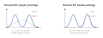
The two directions produce qualitatively different behaviour when the model $q_{θ}$ is not flexible enough to match $p$ exactly:

Forward KL forces

q_{θ}

to cover all modes of

p

(mode-covering), producing a broad, potentially blurry fit. Reverse KL allows

q_{θ}

to concentrate on a single mode (mode-seeking), producing a sharp but incomplete fit.

Key Idea.

Forward KL penalises $q_{θ} (x) \approx 0$ where $p (x) > 0$ . Since $p$ is the reference, any region where $p$ has mass but $q_{θ}$ does not incurs an enormous penalty ( $\log (p / q) \to + \infty$ ). The result is a mode-covering fit: $q_{θ}$ spreads out to cover all modes, even if it fills in the gaps between modes with spurious mass. This explains why MLE-trained models (VAEs) tend to produce blurry outputs.

Reverse KL penalises $q_{θ} (x) > 0$ where $p (x) \approx 0$ . Now $q_{θ}$ is the reference distribution; placing mass outside the support of $p$ incurs $\log (q / p) \to + \infty$ . The model avoids generating anything “unrealistic” but may ignore entire modes. This is mode-seeking behaviour and partially explains GAN mode collapse.

Remark 3 (The Forward/Reverse Divide in Generative Modelling).

This asymmetry creates a deep divide in the field:

Forward KL models (MLE-based): autoregressive models, normalising flows, VAE reconstruction term. These produce diverse but sometimes blurry samples.
Reverse KL / adversarial models: GANs, and the KL term in variational inference. These produce sharp samples but risk mode collapse.

Diffusion models sidestep this divide entirely by using a score-matching objective that does not directly involve either direction of KL (Fisher Divergence and Score Matching).

Jensen–Shannon Divergence

Definition 5 (Jensen–Shannon Divergence).

The Jensen–Shannon (JS) divergence [3] between $P$ and $Q$ is (JS) $\begin{matrix} 𝖣_{JS} (P ‖ Q) = \frac{1}{2} 𝖣_{KL} (P ‖ M) + \frac{1}{2} 𝖣_{KL} (Q ‖ M), M = \frac{1}{2} (P + Q) . \end{matrix}$

JS divergence repairs two deficiencies of KL: it is symmetric ( $𝖣_{JS} (P ‖ Q) = 𝖣_{JS} (Q ‖ P)$ ) and always finite (even when $P$ and $Q$ have disjoint support).

Example 7 (JS Divergence between Two Distributions).

With $P = (0.5, 0.3, 0.2)$ and $Q = (0.1, 0.6, 0.3)$ as in Example 4, the mixture is $M = (0.3, 0.45, 0.25)$ . Then $\begin{matrix} 𝖣_{KL} (P ‖ M) & = 0.5 \log \frac{0.5}{0.3} + 0.3 \log \frac{0.3}{0.45} + 0.2 \log \frac{0.2}{0.25} \approx 0.082, \\ 𝖣_{KL} (Q ‖ M) & = 0.1 \log \frac{0.1}{0.3} + 0.6 \log \frac{0.6}{0.45} + 0.3 \log \frac{0.3}{0.25} \approx 0.088, \\ 𝖣_{JS} (P ‖ Q) & = \frac{1}{2} (0.082 + 0.088) \approx 0.085 nats . \end{matrix}$ Compare this with $𝖣_{KL} (P ‖ Q) \approx 0.516$ : JS divergence is much smaller because it symmetrises and smooths the comparison.

Proposition 3 (Entropy Representation of JS).

(JS Entropy) $\begin{matrix} 𝖣_{JS} (P ‖ Q) = 𝖧 (M) - \frac{1}{2} 𝖧 (P) - \frac{1}{2} 𝖧 (Q), \end{matrix}$ where $𝖧 (\cdot)$ denotes the Shannon entropy and $M = \frac{1}{2} (P + Q)$ .

Proof.

Expand each KL term: $\begin{matrix} 𝖣_{KL} (P ‖ M) & = \sum_{x} P (x) \log \frac{P (x)}{M (x)} = - 𝖧 (P) - \sum_{x} P (x) \log M (x), \\ 𝖣_{KL} (Q ‖ M) & = - 𝖧 (Q) - \sum_{x} Q (x) \log M (x) . \end{matrix}$ Averaging and noting that $\frac{1}{2} \sum_{x} [P (x) + Q (x)] \log M (x) = \sum_{x} M (x) \log M (x) = - 𝖧 (M)$ gives the result.

∎

Theorem 2 (Bounds on JS Divergence).

For any $P, Q$ , (JS Bounds) $\begin{matrix} 0 \leq 𝖣_{JS} (P ‖ Q) \leq \log 2. \end{matrix}$ The lower bound is attained iff $P = Q$ ; the upper bound iff $P$ and $Q$ have disjoint support.

Proof.

The lower bound follows from Gibbs' inequality applied to both KL terms. For the upper bound, when $P$ and $Q$ have disjoint support, every $x$ in the support of $P$ satisfies $M (x) = P (x) / 2$ , so $𝖣_{KL} (P ‖ M) = \log 2$ ; similarly for $Q$ . Hence $𝖣_{JS} = \log 2$ .

∎

Insight.

The original GAN [4] minimises (a function of) the JS divergence between $p_{data}$ and $p_{θ}$ . Goodfellow et al. showed that the optimal discriminator satisfies $D^{*} (x) = \frac{p_{data} (x)}{p_{data} (x) + p_{θ} (x)}$ , and the resulting generator objective equals $2 𝖣_{JS} (p_{data} ‖ p_{θ}) - \log 4$ . The upper bound $𝖣_{JS} \leq \log 2$ being a constant means that when $p_{data}$ and $p_{θ}$ have disjoint support (common early in training when generated images are far from realistic), the gradient of the JS divergence is zero, so the generator receives no learning signal. This is the celebrated “vanishing gradient” problem [5] that motivated the Wasserstein GAN [6] (Chapter 10).

The $f$ -Divergence Family

KL, JS, and total variation are all special cases of a single unified framework.

Historical Note.

The $f$ -divergence was introduced independently by Imre Csiszár [7] in 1963 and by Syed Mumtaz Ali and Samuel Silvey [8] in 1966. Csiszár, a Hungarian information theorist, studied the concept through the lens of information theory, while Ali and Silvey approached it from statistical hypothesis testing. Their independent discovery underscores how naturally the $f$ -divergence framework arises from different mathematical perspectives.

Definition 6 ( $f$ -Divergence).

Let $f : (0, \infty) \to ℝ$ be a convex function with $f (1) = 0$ . The $f$ -divergence [7][8] from $P$ to $Q$ is (F DIV) $\begin{matrix} 𝖣_{f} (P ‖ Q) = 𝔼_{x \sim Q} [f (\frac{P (x)}{Q (x)})] = \sum_{x} Q (x) f (\frac{P (x)}{Q (x)}) . \end{matrix}$ For continuous densities, the sum is replaced by an integral.

Remark 4 (Convention).

Some references define $𝖣_{f} (P ‖ Q) = 𝔼_{P} [f (Q / P)]$ . The two conventions differ by swapping $P$ and $Q$ and/or replacing $f (t)$ with $t f (1 / t)$ (the conjugate generator). We follow the convention $𝔼_{Q} [f (P / Q)]$ , which is standard in the optimal-transport and GAN literature.

Theorem 3 (Non-Negativity of $f$ -Divergence).

$𝖣_{f} (P ‖ Q) \geq 0$ for all $P, Q$ , with equality iff $P = Q$ .

Proof.

By Jensen's inequality (since $f$ is convex): $𝖣_{f} (P ‖ Q) = 𝔼_{Q} [f (\frac{P}{Q})] \geq f (𝔼_{Q} [\frac{P}{Q}]) = f (1) = 0.$

∎

The following table shows how common divergences arise from specific choices of the generator $f$ .

llc@ Divergence	Generator $f (t)$	Symmetric?
KL divergence	$t \log t$	No
Reverse KL	$- \log t$	No
Jensen–Shannon	$t \log t - (1 + t) \log \frac{1 + t}{2}$	Yes
Total variation	$\frac{1}{2} \| t - 1 \|$	Yes
$χ^{2}$ -divergence	${(t - 1)}^{2}$	No
Hellinger distance	${(\sqrt{t} - 1)}^{2}$	Yes

Common divergences as special cases of

f

-divergence with different convex generators.

Example 8 (Deriving KL from $f$ -Divergence).

Choose $f (t) = t \log t$ . Then $𝖣_{f} (P ‖ Q) = 𝔼_{Q} [\frac{P}{Q} \log \frac{P}{Q}] = \sum_{x} P (x) \log \frac{P (x)}{Q (x)} = 𝖣_{KL} (P ‖ Q) .$

Example 9 (Deriving TV from $f$ -Divergence).

Choose $f (t) = \frac{1}{2} | t - 1 |$ . Then $𝖣_{f} (P ‖ Q) = \sum_{x} Q (x) \cdot \frac{1}{2} | \frac{P (x)}{Q (x)} - 1 | = \frac{1}{2} \sum_{x} | P (x) - Q (x) | = 𝖣_{TV} (P, Q) .$

Theorem 4 (Data Processing Inequality).

Let $T$ be any stochastic map (Markov kernel). Then for any $f$ -divergence, (DPI) $\begin{matrix} 𝖣_{f} (T P ‖ T Q) \leq 𝖣_{f} (P ‖ Q) . \end{matrix}$ In words: processing data can only lose information; it can never increase the divergence.

Key Idea.

The data processing inequality has direct consequences for generative modelling:

No post-processing of generated samples (e.g. applying filters, super-resolution) can make them closer in $f$ -divergence to the true data than the raw model output.
$f$ -GAN [9]: Nowozin et al. showed that any $f$ -divergence can be used as a GAN training objective via a variational lower bound. This led to a family of GAN variants using different generators $f$ , generalising the original JS-based GAN.

Total Variation Distance

Definition 7 (Total Variation Distance).

The total variation distance between distributions $P$ and $Q$ is (TV) $\begin{matrix} 𝖣_{TV} (P, Q) = \frac{1}{2} \sum_{x} | P (x) - Q (x) | = \sup_{A \subseteq 𝒳} | P (A) - Q (A) | . \end{matrix}$ For continuous densities, the sum becomes an integral. TV distance is symmetric, satisfies the triangle inequality, and takes values in $[0, 1]$ .

The second expression as a supremum over events has an elegant interpretation: TV distance is the maximum advantage a hypothesis test can gain by choosing the best decision region.

Example 10 (Computing TV Distance).

Let $P = (0.1, 0.3, 0.4, 0.2)$ and $Q = (0.2, 0.2, 0.4, 0.2)$ on ${1,2,3,4}$ . Then $𝖣_{TV} (P, Q) = \frac{1}{2} (| 0.1 - 0.2 | + | 0.3 - 0.2 | + | 0.4 - 0.4 | + | 0.2 - 0.2 |) = \frac{1}{2} (0.1 + 0.1) = 0.1.$ This means that the best possible test to distinguish samples from $P$ versus $Q$ can achieve at most a 10% advantage over random guessing.

Example 11 (TV between Gaussians).

For $P = 𝒩 (0, 1)$ and $Q = 𝒩 (μ, 1)$ (same variance, shifted mean), the TV distance has no simple closed form but can be computed numerically:

$μ$	0.5	1.0	2.0	5.0
$𝖣_{TV} (P, Q)$	0.20	0.38	0.68	0.99

μ = 5

, the distributions are nearly disjoint and TV approaches 1.

The total variation distance is related to KL divergence through an important inequality.

Theorem 5 (Pinsker's Inequality).

For any two distributions $P$ and $Q$ [10], (Pinsker) $\begin{matrix} 𝖣_{TV} (P, Q) \leq \sqrt{\frac{1}{2} 𝖣_{KL} (P ‖ Q)} . \end{matrix}$

Remark 5 (Pinsker in Practice).

Pinsker's inequality provides a useful conceptual bridge: bounding the KL divergence automatically bounds the TV distance. If a model achieves $𝖣_{KL} (p_{data} ‖ p_{θ}) = 0.02$ nats, then $𝖣_{TV} \leq \sqrt{0.01} = 0.1$ , meaning no statistical test can distinguish real from generated samples with more than 10% advantage. This is why small KL values imply good generative quality.

Wasserstein Distance and Optimal Transport

The divergences studied so far (KL, JS, TV) compare distributions point-wise: they depend on the values of $P (x)$ and $Q (x)$ but not on the geometry of the underlying space $𝒳$ . The Wasserstein distance, rooted in optimal transport theory, does account for geometry: moving probability mass a short distance costs less than moving it a long distance.

Historical Note.

The optimal transport problem has a remarkable 240-year history. Gaspard Monge first posed the problem in 1781 [11], not for abstract mathematics, but for a concrete military engineering task: finding the cheapest way to move soil (déblais) to fill fortifications (remblais) during the French Revolution. The problem proved incredibly hard: Monge's formulation requires a deterministic point-to-point assignment, which may not exist.

Over 160 years later, Soviet mathematician Leonid Kantorovich (1942) [12] reformulated the problem by allowing probabilistic transport plans (splitting mass from one source to multiple destinations), turning it into a linear programme. This breakthrough earned him the 1975 Nobel Prize in Economics (for the theory of optimal allocation of resources).

The name “Wasserstein distance” comes from Leonid Vasershtein [13], who used the metric in 1969 to study convergence of Markov chains. The German transliteration of his name (of Yiddish origin, meaning “water stone”) became the standard mathematical term. Computer vision researchers later coined the more intuitive name “earth mover's distance” (EMD) in the 1990s.

The Optimal Transport Problem

Imagine $P$ and $Q$ as two piles of sand of equal total mass, spread over a landscape $𝒳$ . A transport plan $γ (x, y)$ specifies how much mass to move from location $x$ to location $y$ . Any valid plan must satisfy the marginal constraints: the total mass leaving $x$ equals $P (x)$ , and the total mass arriving at $y$ equals $Q (y)$ .

Definition 8 (Wasserstein- $p$ Distance).

Let $(𝒳, d)$ be a metric space and let $P, Q$ be probability measures on $𝒳$ with finite $p$ -th moments ( $p \geq 1$ ). The Wasserstein- $p$ distance is (Wasserstein) $\begin{matrix} W_{p} (P, Q) = {(\inf_{γ \in Π (P, Q)} \int_{𝒳 \times 𝒳} d {(x, y)}^{p} d γ (x, y))}^{1 / p}, \end{matrix}$ where $Π (P, Q)$ is the set of all couplings (joint distributions on $𝒳 \times 𝒳$ with marginals $P$ and $Q$ ).

The Wasserstein distance is the minimum-cost transport plan that reshapes distribution

P

into distribution

Q

. The cost of each “shipment” is proportional to the mass moved times the distance travelled.

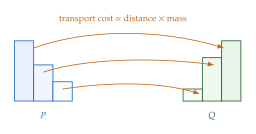
Example 12 (Wasserstein between Point Masses).

For $P = δ_{a}$ and $Q = δ_{b}$ (point masses at $a$ and $b$ on $ℝ$ ), the only coupling is $γ = δ_{(a, b)}$ , giving $W_{p} (P, Q) = | a - b |$ for all $p$ . The Wasserstein distance is simply the Euclidean distance between the two points.

Example 13 (Wasserstein between Univariate Gaussians).

For $P = 𝒩 (μ_{1}, σ_{1}^{2})$ and $Q = 𝒩 (μ_{2}, σ_{2}^{2})$ , the Wasserstein-2 distance has a beautiful closed form: (W2 Gaussian) $\begin{matrix} W_{2} (P, Q) = \sqrt{{(μ_{1} - μ_{2})}^{2} + {(σ_{1} - σ_{2})}^{2}} . \end{matrix}$ This is just the Euclidean distance in the $(μ, σ)$ -parameter space! Compare this with the KL divergence ((KL Gaussian 1D)), which has a more complex, asymmetric form.

Proposition 4 (Wasserstein Distance Is a True Metric).

$W_{p}$ satisfies all properties of a metric: non-negativity, identity of indiscernibles, symmetry, and the triangle inequality. This is a significant advantage over KL and JS divergences.

Proposition 5 (Wasserstein-1 in One Dimension).

For distributions on $ℝ$ with CDFs $F_{P}$ and $F_{Q}$ , the Wasserstein-1 distance has the closed form (W1 1D) $\begin{matrix} W_{1} (P, Q) = \int_{- \infty}^{\infty} | F_{P} (x) - F_{Q} (x) | d x . \end{matrix}$ This is simply the $L^{1}$ distance between the CDFs, the “area between the curves.”

The Kantorovich–Rubinstein Duality

Computing $W_{1}$ from the primal definition requires optimising over all couplings, a challenging task. The following duality theorem provides an alternative characterisation that is far more practical.

Theorem 6 (Kantorovich–Rubinstein Duality).

The Wasserstein-1 distance equals [14] (KR) $\begin{matrix} W_{1} (P, Q) = \sup_{‖ f ‖_{L} \leq 1} [𝔼_{x \sim P} [f (x)] - 𝔼_{x \sim Q} [f (x)]], \end{matrix}$ where the supremum is over all 1-Lipschitz functions $f : 𝒳 \to ℝ$ (i.e. $| f (x) - f (y) | \leq d (x, y)$ for all $x, y$ ).

Insight.

The Kantorovich–Rubinstein duality is the theoretical foundation of the Wasserstein GAN (WGAN) [6], studied in Chapter 10. In WGAN, the discriminator (called the critic) approximates the supremum in (KR): it is a neural network trained to maximise $𝔼_{x \sim p_{data}} [f_{w} (x)] - 𝔼_{z \sim p_{Z}} [f_{w} (g_{θ} (z))]$ subject to a Lipschitz constraint on $f_{w}$ . The generator then minimises the resulting estimate of $W_{1}$ .

Enforcing the Lipschitz constraint in practice remains a challenge. Three main approaches have been proposed:

Weight clipping [6]: clip critic weights to $[- c, c]$ . Simple but can cause the critic to learn only very simple functions.
Gradient penalty (WGAN-GP) [15]: add a penalty $λ 𝔼 [{(‖ \nabla f ‖ - 1)}^{2}]$ to the critic loss. More stable but computationally expensive.
Spectral normalisation [16]: normalise each weight matrix by its spectral norm. Efficient and widely adopted.

Why Wasserstein Distance Matters for GANs

The key advantage of Wasserstein distance over KL and JS for training generative models is its behaviour when distributions have disjoint or low-dimensional support, a situation that is the norm, not the exception, in image generation.

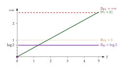
Example 14 (Disjoint Support: KL, JS, TV, and Wasserstein Compared).

Let $P = δ_{0}$ and $Q_{t} = δ_{t}$ be point masses at $0$ and $t$ on $ℝ$ . For $t \neq 0$ : $\begin{matrix} 𝖣_{KL} (P ‖ Q_{t}) & = + \infty, \\ 𝖣_{JS} (P ‖ Q_{t}) & = \log 2 \approx 0.693 (constant), \\ 𝖣_{TV} (P, Q_{t}) & = 1 (constant), \\ W_{1} (P, Q_{t}) & = | t | . \end{matrix}$ Only the Wasserstein distance provides a smooth, meaningful signal: as $t \to 0$ , $W_{1} \to 0$ continuously, while KL divergence remains infinite and JS/TV jump discontinuously from a constant to $0$ .

Divergences between

δ_{0}

and

δ_{t}

as a function of

t

. KL is infinite for all

t \neq 0

; JS and TV are flat constants; only

W_{1}

varies smoothly with

t

, providing useful gradients for optimisation.

Remark 6 (Why Disjoint Support Is the Norm).

Real image distributions are believed to concentrate on a low-dimensional manifold in pixel space (the manifold hypothesis [5]). During GAN training, the generator distribution $p_{θ}$ is also supported on a low-dimensional manifold (the image of the latent space through the network). Two low-dimensional manifolds in a high-dimensional ambient space have measure-zero overlap with probability one. This means KL and JS are essentially useless early in training; their gradients carry no information about which direction to move the generator manifold. Wasserstein distance, by contrast, “sees” the geometric distance between the two manifolds and provides useful gradients throughout.

Caution.

Computing the exact Wasserstein distance in high dimensions is computationally expensive: the primal LP has $O (n^{2})$ variables for $n$ support points, and the dual requires optimising over all Lipschitz functions. The Sinkhorn algorithm [17] (Chapter ch:sinkhorn) provides an efficient entropic regularisation, and neural-network critics approximate the KR dual in WGANs, but both are approximations.

Wasserstein Distance and Weak Convergence

Theorem 7 (Wasserstein Convergence Implies Weak Convergence).

Let ${(μ_{n})}_{n \geq 1}$ be a sequence of probability measures on a metric space $(𝒳, d)$ . If $W_{p} (μ_{n}, μ) \to 0$ for some $p \geq 1$ , then $μ_{n}$ converges weakly to $μ$ : $\int f d μ_{n} \to \int f d μ for all bounded continuous f .$

Proof sketch.

Any bounded Lipschitz function satisfies $| \int f d μ_{n} - \int f d μ | \leq ‖ f ‖_{L} \cdot W_{1} (μ_{n}, μ)$ by the Kantorovich–Rubinstein duality. Since bounded Lipschitz functions are dense (in the sup-norm) among bounded continuous functions on a separable metric space, $W_{1} \to 0$ implies convergence of integrals for all bounded continuous $f$ . The case $p > 1$ follows from the inequality $W_{1} \leq W_{p}$ (by Jensen's).

∎

Remark 7 (Why Weak Convergence Matters for Generative Models).

In generative modelling, we want $p_{θ} \to p_{data}$ in a sense that implies convergence of all expectations, e.g. that generated images “look like” real ones on average. Weak convergence is exactly this notion. Since Wasserstein convergence implies weak convergence, training with $W_{p}$ loss gives meaningful convergence guarantees. By contrast, while $𝖣_{KL} \to 0$ also implies weak convergence (via Pinsker), KL can be infinite when $W_{p}$ is perfectly well-defined.

Mutual Information

Definition 9 (Mutual Information).

The mutual information between random variables $X$ and $Y$ with joint distribution $P_{X Y}$ and marginals $P_{X}, P_{Y}$ is (MI) $\begin{matrix} 𝖨 (X; Y) = 𝖣_{KL} (P_{X Y} ‖ P_{X} \otimes P_{Y}) = 𝔼 [\log \frac{P_{X Y} (x, y)}{P_{X} (x) P_{Y} (y)}] . \end{matrix}$ Equivalently, $𝖨 (X; Y) = 𝖧 (X) - 𝖧 (X | Y) = 𝖧 (Y) - 𝖧 (Y | X)$ .

Mutual information measures how much knowing $Y$ reduces our uncertainty about $X$ (and vice versa). It is zero iff $X$ and $Y$ are independent.

Example 15 (Mutual Information in a Simple Channel).

Consider a binary symmetric channel: $X \sim Bernoulli (0.5)$ and $Y = X \oplus︎ N$ where $N \sim Bernoulli (ϵ)$ is independent noise (flipping $X$ with probability $ϵ$ ). Then $𝖨 (X; Y) = \log 2 - 𝖧 (ϵ) = 1 - 𝖧 (ϵ)$ bits. For a noiseless channel ( $ϵ = 0$ ), $𝖨 = 1$ bit (knowing $Y$ determines $X$ completely). For a completely noisy channel ( $ϵ = 0.5$ ), $𝖨 = 0$ (observing $Y$ tells us nothing about $X$ ).

Key Idea.

Mutual information appears throughout generative modelling:

InfoGAN [18]: the generator is trained to maximise $𝖨 (c; G (z, c))$ between a latent code $c$ and generated output, encouraging disentangled representations, e.g. one dimension of $c$ might control rotation while another controls lighting.
ELBO decomposition: the evidence lower bound in VAEs can be rewritten as $ELBO = 𝔼 [\log p (x)] - 𝖨_{q} (x; z) - 𝖣_{KL} (q (z) ‖ p (z))$ , revealing that the ELBO trades off reconstruction quality against the mutual information between $x$ and $z$ under the encoder $q$ .
Representation learning: good representations should have high mutual information with downstream tasks while discarding irrelevant details (the “information bottleneck” principle).

Fisher Divergence and Score Matching

The divergences discussed so far require evaluating probability densities. The Fisher divergence takes a radically different approach: it compares distributions through their gradients (scores), avoiding the need for normalisation constants entirely.

Definition 10 (Score Function).

The score function (or score) of a distribution with density $p (x)$ is the gradient of the log-density: (Score) $\begin{matrix} s_{p} (x) = \nabla_{x} \log p (x) = \frac{\nabla_{x} p (x)}{p (x)} . \end{matrix}$

The score function points in the direction of steepest ascent of the log-density; intuitively, it points “towards the data.” Crucially, it does not depend on the normalisation constant of $p$ : if $p (x) = \tilde{p} (x) / Z$ , then $\nabla_{x} \log p (x) = \nabla_{x} \log \tilde{p} (x)$ .

Example 16 (Score of a Gaussian).

For $p (x) = 𝒩 (μ, σ^{2})$ , $s_{p} (x) = \frac{d}{d x} [- \frac{{(x - μ)}^{2}}{2 σ^{2}} - \log σ - \frac{1}{2} \log 2 π] = - \frac{x - μ}{σ^{2}} .$ The score points towards the mean $μ$ : positive when $x < μ$ (“go right”) and negative when $x > μ$ (“go left”). Points far from the mean have larger score magnitude; they are “more strongly pulled” towards the centre.

Definition 11 (Fisher Divergence).

The Fisher divergence between distributions $p$ and $q$ is (Fisher) $\begin{matrix} 𝖣_{F} (p ‖ q) = 𝔼_{x \sim p} [{‖ \nabla_{x} \log p (x) - \nabla_{x} \log q (x) ‖}^{2}] = 𝔼_{x \sim p} [‖ s_{p} (x) - s_{q} (x) ‖^{2}] . \end{matrix}$

Example 17 (Fisher Divergence between Gaussians).

For $p = 𝒩 (μ_{1}, σ^{2})$ and $q = 𝒩 (μ_{2}, σ^{2})$ (same variance), $𝖣_{F} (p ‖ q) = 𝔼_{x \sim p} [{(\frac{μ_{2} - μ_{1}}{σ^{2}})}^{2}] = \frac{{(μ_{1} - μ_{2})}^{2}}{σ^{4}} .$ The Fisher divergence is proportional to the squared distance between the means, scaled by the inverse fourth power of the standard deviation; sharper distributions amplify the divergence.

Proposition 6 (Properties of Fisher Divergence).

$𝖣_{F} (p ‖ q) \geq 0$ , with equality iff $p = q$ (under mild regularity conditions).
$𝖣_{F}$ does not require computing the normalisation constants of $p$ or $q$ , only their score functions.
$𝖣_{F}$ involves only first-order derivatives, making it amenable to gradient-based optimisation.

Score Matching

Directly computing $𝖣_{F} (p_{data} ‖ q_{θ})$ requires access to $s_{p_{data}} (x) = \nabla_{x} \log p_{data} (x)$ , which we do not know. Hyvärinen's score matching objective [19] circumvents this via integration by parts.

Theorem 8 (Hyvärinen's Score Matching Identity).

Under suitable regularity conditions (in particular, $p (x) s_{q_{θ}} (x) \to 0$ as $‖ x ‖ \to \infty$ ), (Score Matching) $\begin{matrix} 𝖣_{F} (p ‖ q_{θ}) = 𝔼_{x \sim p} [trace (\nabla_{x} s_{q_{θ}} (x)) + \frac{1}{2} ‖ s_{q_{θ}} (x) ‖^{2}] + C, \end{matrix}$ where $C$ is a constant independent of $θ$ and $\nabla_{x} s_{q_{θ}}$ is the Jacobian of the model's score [19].

The key point is that the right-hand side depends only on the model's score $s_{q_{θ}}$ and samples from the data; we never need to know $s_{p_{data}}$ explicitly.

Denoising Score Matching

In practice, computing $trace (\nabla_{x} s_{q_{θ}})$ is expensive in high dimensions (it requires computing diagonal entries of the Jacobian). Vincent [22] showed that adding noise provides a much cheaper alternative.

Theorem 9 (Denoising Score Matching).

Let $\tilde{x} = x + σ ϵ$ with $ϵ \sim 𝒩 (0, I)$ . Define the noised density $p_{σ} (\tilde{x}) = \int p (x) 𝒩 (\tilde{x}; x, σ^{2} I) d x$ . Then (DSM) $\begin{matrix} {arg min}_{θ} 𝔼_{x \sim p} 𝔼_{ϵ \sim 𝒩 (0, I)} [{‖ s_{θ} (\tilde{x}) + \frac{ϵ}{σ} ‖}^{2}] = {arg min}_{θ} 𝖣_{F} (p_{σ} ‖ q_{θ}) . \end{matrix}$ At the optimal $θ$ , $s_{θ} (\tilde{x}) \approx \nabla_{\tilde{x}} \log p_{σ} (\tilde{x})$ .

Key Idea.

Score matching is the foundation of diffusion models. Song and Ermon [20] showed that training a neural network $s_{θ} (x, σ)$ to estimate the score at multiple noise levels $σ$ enables generation via annealed Langevin dynamics: starting from pure noise and gradually reducing $σ$ while following the estimated score.

Ho et al. [21] (DDPM) showed that this is equivalent to training a denoiser $ϵ_{θ} (x_{t}, t)$ that predicts the noise added at each diffusion step, the connection being $s_{θ} (x_{t}, t) = - ϵ_{θ} (x_{t}, t) / σ_{t}$ . The entire training pipeline of modern diffusion models (Stable Diffusion, DALL-E, etc.) rests on the Fisher divergence and denoising score matching.

Choosing a Divergence for Generative Modelling

Each divergence has strengths and weaknesses. tab:divergence-comparison summarises the trade-offs.

lcccl@ Divergence	Metric?	Disjoint OK?	Needs density?	Used by
$𝖣_{KL}$ (fwd)	No	No ( $= \infty$ )	Yes	MLE, VAE
$𝖣_{KL}$ (rev)	No	No ( $= \infty$ )	Yes	VI, wake-sleep
$𝖣_{JS}$	No	Finite but flat	Yes	Original GAN
$𝖣_{TV}$	Yes	Finite but flat	Yes	Theory
$W_{1}$ (Wasserstein)	Yes	Yes (smooth)	No	WGAN
$𝖣_{F}$ (Fisher)	No	N/A (uses scores)	Scores only	Diffusion

Comparison of divergences for generative modelling. “Disjoint OK?” indicates behaviour when

P

and

Q

have non-overlapping support. “Needs density?” indicates whether evaluating

p (x)

q (x)

is required.

Remark 8 (No Single Best Divergence).

There is no universally “best” divergence. The choice depends on the model architecture and the computational budget:

If the model provides a tractable density (autoregressive, flow), use forward KL (MLE).
If the model is implicit (GAN), use Wasserstein or JS.
If the model is a score network (diffusion), use Fisher divergence via denoising score matching.
For variational inference with an approximate posterior, use reverse KL.

Understanding why each model uses a particular divergence is the key to understanding its strengths and failure modes.

Remark 9 (A Curious Unification).

It is a remarkable fact that the seemingly different training objectives used by GANs, VAEs, and diffusion models can all be understood as minimising different divergences between the same pair of distributions. The entire landscape of modern generative modelling can be organised by the single question: which divergence are you minimising? This chapter gives you the vocabulary to answer that question for any model you encounter.

Exercises

Exercise 1 (Non-Negativity of KL via Jensen's Inequality).

Prove that $𝖣_{KL} (P ‖ Q) \geq 0$ using Jensen's inequality applied to the concave function $\log$ . When does equality hold?

Exercise 2 (KL between Discrete Distributions).

Let $P = (0.5, 0.3, 0.2)$ and $Q = (0.1, 0.6, 0.3)$ on ${1, 2, 3}$ . Compute: (a) $𝖣_{KL} (P ‖ Q)$ , (b) $𝖣_{KL} (Q ‖ P)$ , (c) $𝖣_{JS} (P ‖ Q)$ , and (d) $𝖣_{TV} (P, Q)$ . Verify that $𝖣_{KL} (P ‖ Q) \neq 𝖣_{KL} (Q ‖ P)$ .

Exercise 3 (KL between Univariate Gaussians).

Let $P = 𝒩 (μ_{1}, σ_{1}^{2})$ and $Q = 𝒩 (μ_{2}, σ_{2}^{2})$ . Derive the closed-form expression . Specialise to $σ_{1} = σ_{2} = σ$ and interpret the result geometrically.

Exercise 4 (JS Entropy Representation).

Prove that $𝖣_{JS} (P ‖ Q) = 𝖧 (M) - \frac{1}{2} 𝖧 (P) - \frac{1}{2} 𝖧 (Q)$ where $M = \frac{1}{2} (P + Q)$ . Use this to show $0 \leq 𝖣_{JS} \leq \log 2$ .

Exercise 5 (Disjoint Support).

Let $P$ and $Q$ have disjoint supports. Compute $𝖣_{KL} (P ‖ Q)$ , $𝖣_{JS} (P ‖ Q)$ , $𝖣_{TV} (P, Q)$ , and $W_{1} (P, Q)$ (for $P = δ_{0}$ , $Q = δ_{t}$ on $ℝ$ ). Explain why only Wasserstein provides a useful gradient signal for training.

Exercise 6 (TV as $f$ -Divergence).

Show that $𝖣_{TV} (P, Q) = 𝖣_{f} (P ‖ Q)$ with generator $f (t) = \frac{1}{2} | t - 1 |$ . Verify that $f$ is convex and $f (1) = 0$ .

Exercise 7 (Pinsker's Inequality Application).

A model achieves $𝖣_{KL} (p_{data} ‖ p_{θ}) = 0.02$ nats. Use Pinsker's inequality to bound the total variation distance. If you have $n = 10,000$ test samples, approximately how many would you expect to be “misclassified” by a hypothesis test between $p_{data}$ and $p_{θ}$ ?

Exercise 8 (Data Processing Inequality).

Let $P$ and $Q$ be distributions on images, and let $T$ be a Gaussian blur operator. Explain intuitively why $𝖣_{f} (T P ‖ T Q) \leq 𝖣_{f} (P ‖ Q)$ . What does this imply about evaluating generative models using blurred images?

Exercise 9 (Kantorovich–Rubinstein in Practice).

Explain why the Kantorovich–Rubinstein duality ((KR)) requires $f$ to be 1-Lipschitz rather than merely bounded. In WGAN, the critic network $f_{w}$ is constrained to be approximately 1-Lipschitz. Describe two practical methods for enforcing this constraint and discuss their trade-offs.

Exercise 10 (Score Matching Derivation).

Starting from $𝖣_{F} (p ‖ q_{θ}) = 𝔼_{p} [‖ s_{p} - s_{q_{θ}} ‖^{2}]$ , expand the square and use integration by parts to derive Hyvärinen's identity . State clearly the boundary conditions needed for the integration by parts to work.

Exercise 11 (Forward vs. Reverse KL).

Let $p (x) = 0.5 𝒩 (- 3, 0.5) + 0.5 𝒩 (3, 0.5)$ be a bimodal distribution, and let $q_{θ} = 𝒩 (μ, σ^{2})$ be a single Gaussian.

Find ${arg min}_{μ, σ^{2}} 𝖣_{KL} (p ‖ q_{θ})$ (forward KL). Describe the fitted $q_{θ}$ .
Argue qualitatively what ${arg min}_{μ, σ^{2}} 𝖣_{KL} (q_{θ} ‖ p)$ (reverse KL) looks like.
Relate your findings to the mode-covering vs. mode-seeking behaviour discussed in Forward vs. Reverse KL Divergence.

Exercise 12 (Mutual Information and Independence).

Prove that $𝖨 (X; Y) \geq 0$ with equality iff $X$ and $Y$ are independent. Then show that $𝖨 (X; Y) = 𝖧 (X) + 𝖧 (Y) - 𝖧 (X, Y)$ and use this to argue that mutual information measures the “redundancy” between $X$ and $Y$ .

Exercise 13 (Comparing Divergences Numerically).

Let $P = 𝒩 (0, 1)$ and $Q_{t} = 𝒩 (t, 1)$ for $t \in {0, 0.5, 1, 2, 5}$ . Compute $𝖣_{KL} (P ‖ Q_{t})$ , $W_{2} (P, Q_{t})$ , and $𝖣_{F} (P ‖ Q_{t})$ for each value of $t$ using the closed-form expressions derived in this chapter. Hint: For equal-variance Gaussians, $𝖣_{KL} = {(μ_{1} - μ_{2})}^{2} / (2 σ^{2})$ , $W_{2} = | μ_{1} - μ_{2} |$ , and $𝖣_{F} = {(μ_{1} - μ_{2})}^{2} / σ^{4}$ . Plot all three as functions of $t$ and discuss their different scaling behaviours.

Exercise 14 (Wasserstein between Gaussians).

Verify (W2 Gaussian): for $P = 𝒩 (0, 1)$ and $Q = 𝒩 (2, 4)$ , compute $W_{2} (P, Q)$ using the closed form. Compare with $𝖣_{KL} (P ‖ Q)$ and comment on which measure is more “geometrically natural.”

References

A mathematical theory of communication

Claude Elwood Shannon

The Bell System Technical Journal, vol. 27, no. 3, pp. 379-423 · 1948

BibTeX

@article{shannon1948mathematical,
  title={A mathematical theory of communication},
  author={Shannon, Claude Elwood},
  journal={The Bell System Technical Journal},
  volume={27},
  number={3},
  pages={379--423},
  year={1948},
  publisher={Nokia Bell Labs}
}

Journal article

On information and sufficiency

Solomon Kullback, Richard A Leibler

The annals of mathematical statistics, vol. 22, no. 1, pp. 79-86 · 1951

BibTeX

@article{kullback1951information,
  title={On information and sufficiency},
  author={Kullback, Solomon and Leibler, Richard A},
  journal={The annals of mathematical statistics},
  volume={22},
  number={1},
  pages={79--86},
  year={1951},
  publisher={Institute of Mathematical Statistics}
}

Journal article

Divergence measures based on the Shannon entropy

Jianhua Lin

IEEE Transactions on Information theory, vol. 37, no. 1, pp. 145-151 · 1991

BibTeX

@article{lin1991divergence,
  title={Divergence measures based on the Shannon entropy},
  author={Lin, Jianhua},
  journal={IEEE Transactions on Information theory},
  volume={37},
  number={1},
  pages={145--151},
  year={1991},
  publisher={IEEE}
}

Journal article

Generative Adversarial Networks

Ian Goodfellow, Jean Pouget-Abadie, Mehdi Mirza, Bing Xu, David Warde-Farley, Sherjil Ozair, Aaron Courville, Yoshua Bengio

Advances in Neural Information Processing Systems, vol. 27 · 2014

BibTeX

@inproceedings{goodfellow2014generative,
  title={Generative Adversarial Networks},
  author={Goodfellow, Ian and Pouget-Abadie, Jean and Mirza, Mehdi and Xu, Bing and Warde-Farley, David and Ozair, Sherjil and Courville, Aaron and Bengio, Yoshua},
  booktitle={Advances in Neural Information Processing Systems},
  volume={27},
  year={2014}
}

Conference paper

Towards principled methods for training generative adversarial networks

Martin Arjovsky, Leon Bottou

arXiv preprint arXiv:1701.04862 · 2017

BibTeX

@article{arjovsky2017towards,
  title={Towards principled methods for training generative adversarial networks},
  author={Arjovsky, Martin and Bottou, L{\'e}on},
  journal={arXiv preprint arXiv:1701.04862},
  year={2017}
}

Journal article

Wasserstein GAN

Martin Arjovsky, Soumith Chintala, Leon Bottou

arXiv:1701.07875 · 2017

BibTeX

@article{arjovsky2017wasserstein,
    title = {Wasserstein GAN},
    author = {Arjovsky, Martin and Chintala, Soumith and Bottou, L\'eon},
    journal = {arXiv:1701.07875},
    year = {2017}
}

Journal article

Eine informationstheoretische Ungleichung und ihre Anwendung auf den Beweis der Ergodizitat von Markoffschen Ketten

Imre Csiszar

Magyar Tud. Akad. Mat. Kutato Int. Kozl, vol. 8, pp. 85-108 · 1963

BibTeX

@article{csiszar1963information,
  title={Eine informationstheoretische Ungleichung und ihre Anwendung auf den Beweis der Ergodizit{\"a}t von Markoffschen Ketten},
  author={Csisz{\'a}r, Imre},
  journal={Magyar Tud. Akad. Mat. Kutat{\'o} Int. K{\"o}zl},
  volume={8},
  pages={85--108},
  year={1963}
}

Journal article

A general class of coefficients of divergence of one distribution from another

Syed Mumtaz Ali, Samuel D. Silvey

Journal of the Royal Statistical Society: Series B (Methodological), vol. 28, no. 1, pp. 131-142 · 1966

BibTeX

@article{ali1966general,
  title={A general class of coefficients of divergence of one distribution from another},
  author={Ali, Syed Mumtaz and Silvey, Samuel D.},
  journal={Journal of the Royal Statistical Society: Series B (Methodological)},
  volume={28},
  number={1},
  pages={131--142},
  year={1966}
}

Journal article

f-GAN: Training generative neural samplers using variational divergence minimization

Sebastian Nowozin, Botond Cseke, Ryota Tomioka

Advances in Neural Information Processing Systems, vol. 29 · 2016

BibTeX

@inproceedings{nowozin2016fgan,
  title={f-GAN: Training generative neural samplers using variational divergence minimization},
  author={Nowozin, Sebastian and Cseke, Botond and Tomioka, Ryota},
  booktitle={Advances in Neural Information Processing Systems},
  volume={29},
  year={2016}
}

Conference paper

Information and Information Stability of Random Variables and Processes

Mark S. Pinsker

Holden-Day · 1964

BibTeX

@book{pinsker1964information,
  title={Information and Information Stability of Random Variables and Processes},
  author={Pinsker, Mark S.},
  publisher={Holden-Day},
  year={1964},
  address={San Francisco}
}

Book

Memoire sur la theorie des deblais et des remblais

Gaspard Monge

Memoires de l'Academie Royale des Sciences de Paris, pp. 666-704 · 1781

BibTeX

@article{monge1781memoire,
  title={M{\'e}moire sur la th{\'e}orie des d{\'e}blais et des remblais},
  author={Monge, Gaspard},
  journal={M{\'e}moires de l'Acad{\'e}mie Royale des Sciences de Paris},
  pages={666--704},
  year={1781}
}

Journal article

On the translocation of masses

L. V. Kantorovich

C. R. (Doklady) Acad. Sci. URSS (N.S.), vol. 37, pp. 199-201 · 1942

BibTeX

@article{kantorovich1942translocation,
  title={On the translocation of masses},
  author={Kantorovich, L. V.},
  journal={C. R. (Doklady) Acad. Sci. URSS (N.S.)},
  volume={37},
  pages={199--201},
  year={1942}
}

Journal article

Markov processes over denumerable products of spaces, describing large systems of automata

Leonid N. Vasershtein

Problemy Peredachi Informatsii, vol. 5, no. 3, pp. 64-72 · 1969

BibTeX

@article{vasershtein1969markov,
  title={Markov processes over denumerable products of spaces, describing large systems of automata},
  author={Vasershtein, Leonid N.},
  journal={Problemy Peredachi Informatsii},
  volume={5},
  number={3},
  pages={64--72},
  year={1969}
}

Journal article

Optimal Transport: Old and New

Cedric Villani

Springer-Verlag · 2008

BibTeX

@book{villani2008optimal,
    title = {Optimal Transport: Old and New},
    author = {Villani, C\'edric},
    year = {2008},
    publisher = {Springer-Verlag}
}

Book

Improved training of Wasserstein GANs

Ishaan Gulrajani, Faruk Ahmed, Martin Arjovsky, Vincent Dumoulin, Aaron C Courville

Advances in neural information processing systems, pp. 5767-5777 · 2017

BibTeX

@inproceedings{gulrajani2017improved,
  title={Improved training of Wasserstein GANs},
  author={Gulrajani, Ishaan and Ahmed, Faruk and Arjovsky, Martin and Dumoulin, Vincent and Courville, Aaron C},
  booktitle={Advances in neural information processing systems},
  pages={5767--5777},
  year={2017}
}

Conference paper

Spectral normalization for generative adversarial networks

Takeru Miyato, Toshiki Kataoka, Masanori Koyama, Yuichi Yoshida

Proceedings of the International Conference on Learning Representations · 2018

BibTeX

@inproceedings{miyato2018spectral,
  title={Spectral normalization for generative adversarial networks},
  author={Miyato, Takeru and Kataoka, Toshiki and Koyama, Masanori and Yoshida, Yuichi},
  booktitle={Proceedings of the International Conference on Learning Representations},
  year={2018},
  url={https://openreview.net/forum?id=B1QRgziT-}
}

Conference paper

Sinkhorn Distances: Lightspeed Computation of Optimal Transport

Marco Cuturi

Advances in Neural Information Processing Systems · 2013

BibTeX

@inproceedings{cuturi2013sinkhorn,
  title={Sinkhorn Distances: Lightspeed Computation of Optimal Transport},
  author={Cuturi, Marco},
  booktitle={Advances in Neural Information Processing Systems},
  year={2013}
}

Conference paper

InfoGAN: Interpretable representation learning by information maximizing generative adversarial nets

Xi Chen, Yan Duan, Rein Houthooft, John Schulman, Ilya Sutskever, Pieter Abbeel

Advances in Neural Information Processing Systems, vol. 29 · 2016

BibTeX

@inproceedings{chen2016infogan,
  title={InfoGAN: Interpretable representation learning by information maximizing generative adversarial nets},
  author={Chen, Xi and Duan, Yan and Houthooft, Rein and Schulman, John and Sutskever, Ilya and Abbeel, Pieter},
  booktitle={Advances in Neural Information Processing Systems},
  volume={29},
  year={2016}
}

Conference paper

Estimation of non-normalized statistical models by score matching

Aapo Hyvarinen

Journal of Machine Learning Research, vol. 6, pp. 695-709 · 2005

BibTeX

@article{hyvarinen2005estimation,
  title={Estimation of non-normalized statistical models by score matching},
  author={Hyv{\"a}rinen, Aapo},
  journal={Journal of Machine Learning Research},
  volume={6},
  pages={695--709},
  year={2005}
}

Journal article

Generative modeling by estimating gradients of the data distribution

Yang Song, Stefano Ermon

Advances in Neural Information Processing Systems, vol. 32 · 2019

BibTeX

@inproceedings{song2019generative,
  title={Generative modeling by estimating gradients of the data distribution},
  author={Song, Yang and Ermon, Stefano},
  booktitle={Advances in Neural Information Processing Systems},
  volume={32},
  year={2019}
}

Conference paper

Denoising Diffusion Probabilistic Models

Jonathan Ho, Ajay Jain, Pieter Abbeel

Advances in Neural Information Processing Systems, vol. 33, pp. 6840-6851 · 2020

BibTeX

@inproceedings{ho2020denoising,
  title={Denoising Diffusion Probabilistic Models},
  author={Ho, Jonathan and Jain, Ajay and Abbeel, Pieter},
  booktitle={Advances in Neural Information Processing Systems},
  volume={33},
  pages={6840--6851},
  year={2020}
}

Conference paper

A connection between score matching and denoising autoencoders

Pascal Vincent

Neural Computation, vol. 23, no. 7, pp. 1661-1674 · 2011

BibTeX

@article{vincent2011connection,
  title={A connection between score matching and denoising autoencoders},
  author={Vincent, Pascal},
  journal={Neural Computation},
  volume={23},
  number={7},
  pages={1661--1674},
  year={2011}
}

Journal article

← 3 Foundations of Generative Modelling 5 Deep Learning Building Blocks →

4 Divergence Measures and Information Theory

Entropy and Cross-Entropy

Kullback–Leibler Divergence

KL Divergence between Gaussians

Forward vs. Reverse KL Divergence

Jensen–Shannon Divergence

The f-Divergence Family

Total Variation Distance

Wasserstein Distance and Optimal Transport

The Optimal Transport Problem

The Kantorovich–Rubinstein Duality

Why Wasserstein Distance Matters for GANs

Wasserstein Distance and Weak Convergence

Mutual Information

Fisher Divergence and Score Matching

Score Matching

Denoising Score Matching

Choosing a Divergence for Generative Modelling

Exercises

References

The $f$ -Divergence Family