15 Variational Autoencoders
The previous chapters of this book developed two families of generative models. Gaussian mixture models (Chapter 7) introduced latent variable modelling and the expectation–maximisation algorithm for discrete latent spaces. Generative adversarial networks (Chapters 9–13) showed how to train implicit generators through adversarial games. In this chapter we combine neural networks with variational inference to build the Variational Autoencoder (VAE), a principled framework for learning deep latent variable models.
The journey proceeds in five steps:
We start with deterministic autoencoders and their connection to PCA.
We introduce deep latent variable models and explain why the posterior is intractable.
We derive the Evidence Lower Bound (ELBO) from two complementary perspectives.
We assemble the VAE: an amortised encoder, a neural decoder, and the reparameterisation trick for end-to-end training.
We discuss practical issues: posterior collapse, latent space structure, and generation quality.
Historical Note.
The VAE was independently proposed by Kingma & Welling [1] and Rezende, Mohamed & Wierstra [2] in 2013–2014. The key insight, amortising variational inference with a neural-network encoder and training end-to-end via the reparameterisation trick, unified Bayesian latent-variable modelling with deep learning and opened the door to scalable generative models of images, text, and molecules.
Autoencoders
Before introducing the probabilistic machinery of VAEs, we review their deterministic predecessor: the autoencoder.
Definition 1 (Autoencoder).
An autoencoder consists of
an encoder , and
a decoder ,
with bottleneck dimension . The pair is trained to minimise a reconstruction loss over a dataset : (Recon LOSS)
The encoder compresses each input into a latent code ; the decoder attempts to reconstruct from . Because , the bottleneck forces the network to discover a compact representation that captures the most important structure of the data.

Autoencoders find applications in dimensionality reduction, denoising (by training on corrupted inputs), feature learning, and anomaly detection (by flagging inputs with high reconstruction error). However, they suffer from a fundamental limitation for generative modelling.
Key Idea.
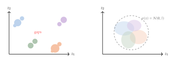
A deterministic autoencoder learns to compress and reconstruct, but its latent space has no guaranteed structure. Sampling a random and decoding it may produce nonsense, because nothing forces the encoder's outputs to fill the latent space in a regular way. The VAE solves this by imposing a probabilistic prior on the latent space.
Linear Autoencoders and PCA
We now make precise the connection between autoencoders and the classical technique of Principal Component Analysis (PCA). Recall that PCA projects data onto the top eigenvectors of the covariance matrix , thereby minimising the reconstruction error among all linear projections.
Definition 2 (Linear Autoencoder).
A linear autoencoder is an autoencoder whose encoder and decoder use only linear transformations (no activation functions): with , and with .
Theorem 1 (Linear Autoencoder – PCA Equivalence).
Let and minimise the reconstruction loss over centred data (). Then at any global minimum, where contains the top eigenvectors of the data covariance matrix .
Proof.
Let be the centred data matrix (rows are data points). The reconstruction loss equals where has rank at most . Minimising over all rank- matrices is precisely the Eckart–Young problem. Let be the (thin) SVD. The Eckart–Young theorem gives , where consists of the top right singular vectors of . Since , the right singular vectors of are precisely the eigenvectors of (ordered by eigenvalue). Any factorisation of rank satisfies .
Insight.
PCA is the best that any linear model can do. A nonlinear autoencoder (with ReLU or other activations) can capture curved manifolds that PCA misses entirely. The VAE goes further: it adds probabilistic structure on top of this nonlinear capability, enabling principled generation and density estimation.
Latent Variable Models
We now shift from deterministic compression to probabilistic generative modelling. The central idea is to posit a latent (unobserved) variable that explains the observed data through a generative process: first sample from a simple prior, then generate conditioned on .
Definition 3 (Deep Latent Variable Model).
A deep latent variable model defines a joint distribution (Joint) where
is the prior over latent variables , and
is the likelihood (decoder), parameterised by a neural network with parameters .
The marginal likelihood (evidence) is (Marginal)
This framework generalises the Gaussian mixture model studied in Exercise 14: in a GMM the latent variable is discrete (the cluster label) and the decoder is a simple Gaussian . The deep LVM replaces the discrete with a continuous Gaussian and the simple decoder with a neural network, vastly increasing expressiveness.
The goal is to find parameters that maximise the log-likelihood of the observed data: (MLE) This is equivalent to minimising the KL divergence (cf. Definition 3).
Proposition 1 (Intractable Posterior).
For a deep latent variable model with a nonlinear neural-network decoder, the posterior (Posterior) is intractable: computing the denominator requires evaluating the decoder network at every point in the latent space, an integral that has no closed-form solution in general.
Proof.
Evaluating requires integrating the product of a standard Gaussian density and the nonlinear function over . When the decoder is a multi-layer neural network, this product is a highly multimodal function of for which no analytic antiderivative exists. Moreover, naïve Monte Carlo estimation (sampling ) suffers from exponentially high variance in high dimensions, since most samples from the prior land in regions where is negligible.
Caution.
The intractability of means we cannot directly compute the log-likelihood, its gradients, or the posterior. Every technique in the rest of this chapter (the ELBO, amortised inference, the reparameterisation trick) is a creative response to this fundamental barrier.
The Evidence Lower Bound
Since maximising directly is intractable, we introduce an approximate posterior and derive a tractable lower bound on the log-evidence. We present two derivations that reveal complementary insights.
Jensen Derivation
Theorem 2 (Evidence Lower Bound - Jensen).
For any distribution with wherever , (ELBO Jensen) The quantity is called the evidence lower bound (ELBO).
Proof.
Starting from the marginal likelihood: where the last step applies Jensen's inequality ( is concave).
The ELBO decomposes naturally into two interpretable terms.
Proposition 2 (ELBO Decomposition).
(ELBO Decompose)
Proof.
Expanding the log ratio inside the ELBO:
The reconstruction term encourages and to explain the data well; the KL term penalises for deviating from the prior. This tension between fidelity and regularity is the defining feature of variational methods.
Bayes Derivation
The second derivation reveals the gap between the ELBO and the true log-evidence.
Theorem 3 (ELBO Gap Identity).
(ELBO GAP) The gap between the ELBO and the log-evidence is precisely the KL divergence between the approximate posterior and the true posterior .
Proof.
We start from the KL divergence between and the true posterior: Rearranging gives .
Since , we immediately recover the lower-bound property . More importantly, the gap identity tells us exactly when the bound is tight.
Key Idea.
The two ELBO derivations reveal complementary insights:
The Jensen derivation shows that is a lower bound on .
The Bayes derivation shows that maximising over simultaneously pushes towards the true posterior and increases the log-evidence.
When , the bound is tight: .
Remark 1 (Connection to GMM ELBO).
The ELBO was first encountered in the context of Gaussian mixture models (EM as Coordinate Ascent on the ELBO), where assigns each data point to a mixture component. The EM algorithm alternates between tightening the bound (E-step) and maximising it (M-step). The VAE replaces these discrete updates with gradient-based optimisation of continuous encoder and decoder parameters.
The VAE Architecture
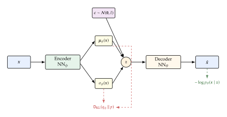
Classical variational inference optimises a separate for each data point , which is computationally expensive for large datasets. The VAE introduces amortised inference: a single neural network, called the encoder or inference network, maps any to the parameters of an approximate posterior .
Definition 4 (Variational Autoencoder).
A variational autoencoder consists of three components:
An encoder (inference network) , where and are outputs of a neural network with parameters .
A decoder (generative network) , parameterised by a neural network with parameters .
A prior .
The VAE is trained by maximising the ELBO summed (or averaged) over the dataset. Using the amortised posterior in place of a generic , the VAE objective becomes:
(Objective)
Remark 2 (Amortised Inference).
In classical variational inference, one optimises a separate variational distribution for each data point , requiring an inner optimisation loop. The VAE amortises this cost: the encoder shares parameters across all data points, so the cost of inference is a single forward pass through the network. This makes the VAE scalable to millions of data points.
Remark 3 (Reconstruction Loss).
The form of determines the reconstruction loss:
Gaussian decoder: yields MSE loss: .
Bernoulli decoder: yields binary cross-entropy loss (suitable for binary or normalised images).
Gaussian VAE: Closed-Form KL Divergence
A major computational advantage of the Gaussian VAE is that the KL term in the ELBO can be evaluated in closed form. The general KL divergence between multivariate Gaussians was derived in Proposition 2; here we specialise to the diagonal-covariance case that arises in the standard VAE.
Theorem 4 (Closed-Form KL for Gaussian VAE).
Let with and , and let . Then (KL Gaussian)
Proof.
Step 1 (Factorisation). Because both and factorise across dimensions ( and ), the KL divergence decomposes: (KL Factorise)
Step 2 (Per-dimension KL). For a single dimension, and : (KL 1D)
Step 3 (Combine). Summing over dimensions and writing :
Insight.
The closed-form KL term is the reason VAEs almost universally use Gaussian encoders with a standard normal prior. No Monte Carlo estimation is needed for the regularisation term; only the reconstruction term requires sampling, making training significantly more stable.
Substituting the closed-form KL and a single-sample Monte Carlo estimate for the reconstruction term, the practical VAE loss for a minibatch becomes:
(FULL LOSS) where with .
The Reparameterisation Trick in VAEs
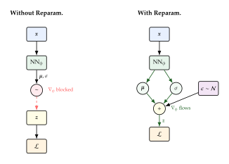
The ELBO involves the expectation . To maximise with gradient-based optimisation, we need of this expectation. However, naïvely sampling creates a stochastic node that blocks gradient flow: the sample depends on , but the sampling operation is not differentiable.
The solution is the reparameterisation trick, introduced in Definition 5 (Chapter 3). Here we show how it applies specifically to the VAE.
Proposition 3 (Reparameterised ELBO Gradient).
Using the reparameterisation with , the gradient of the reconstruction term can be computed as: (Reparam Gradient)
Proof.
Define the deterministic function . By the law of the unconscious statistician (LOTUS), if with , then for any measurable . Applying this with and noting that does not depend on : where the interchange of gradient and expectation is justified because is independent of (Leibniz's rule).
Remark 4 (Single-Sample Estimator).
In practice, a single Monte Carlo sample () per data point suffices when using large minibatches. This is the approach used in the original VAE paper [1]: the variance from using is offset by averaging over many data points in the minibatch.
VAE Training Algorithm
We now consolidate the preceding results into complete training and sampling algorithms.
Algorithm 1 (VAE Training).
Input: Dataset , latent dimension , learning rate , epochs , minibatch size . Output: Trained parameters .
Initialise encoder parameters and decoder parameters randomly.
for do
Randomly shuffle the dataset into minibatches of size .
for each minibatch do
for do
Compute and via the encoder.
Sample .
Set .
end for
Evaluate the minibatch ELBO: .
Update ; .
end for
end for
Algorithm 2 (Sampling from a Trained VAE).
Input: Trained decoder , number of samples . Output: Generated samples .
for do
Sample .
Compute (or sample ).
end for
Remark 5 (Implementation Details).
Several practical considerations arise when implementing VAEs:
Log-variance parameterisation. The encoder should output rather than directly. This avoids the need for a positivity constraint and is numerically more stable.
Optimiser. Adam [3] is the standard choice, typically with learning rate .
Latent dimension. Common choices range from (for visualisation) to or higher (for complex image generation).
Architecture. Convolutional encoders/decoders are standard for images; fully connected networks suffice for low-dimensional tabular data.
Posterior Collapse
One of the most common failure modes in VAE training occurs when the encoder learns to ignore the input, making the approximate posterior match the prior on some or all latent dimensions.
Definition 5 (Posterior Collapse).
Posterior collapse occurs when, for some latent dimension , the approximate posterior matches the prior for all data points: In this regime, the encoder ignores the input along dimension (, ), and the decoder receives no useful information from .
Posterior collapse arises from the tension between the two ELBO terms. The KL term is minimised when (yielding ), while the reconstruction term benefits from an informative posterior. If the decoder is powerful enough to model the data distribution without relying on (for example, an autoregressive decoder such as PixelCNN), then the “easiest” solution is to set and let the decoder do all the work.
Caution.
Posterior collapse is not merely a theoretical curiosity; it is one of the most common failure modes when training VAEs in practice. Especially with powerful autoregressive decoders (PixelCNN, Transformer), the model can learn to ignore the latent variable entirely, reducing the VAE to a standard autoregressive model with wasted latent dimensions.
Several mitigation strategies have been proposed:
KL annealing (warm-up): During early training, weight the KL term by a factor that increases from to over the first several epochs. This gives the encoder time to learn useful representations before the full regularisation pressure is applied [4].
Free bits: Replace with per dimension, ensuring that each latent dimension carries at least nats of information [5].
-VAE weighting: Use with to reduce the regularisation pressure, at the cost of less structured latent spaces.
Remark 6 (-VAE).
The -VAE [6] introduces a hyperparameter before the KL term: . When , the stronger regularisation encourages disentangled representations where each latent dimension captures a single generative factor. A full treatment of the -VAE and its variants appears in the next chapter.
Latent Space Structure and Generation Quality
The KL regularisation term in the ELBO endows the VAE's latent space with useful geometric properties that deterministic autoencoders lack.
Example 1 (Latent Space Interpolation).
Given two data points and , encode them to obtain and . Decoding the linear interpolation for produces a smooth transition between and in data space. This property arises because the KL term ensures that the latent space has no “holes” between encoded data points. Deterministic autoencoders do not guarantee this; interpolated points may land in regions where the decoder has never been trained.
Remark 7 (Generation Quality: VAE vs. GAN).
VAE-generated samples are often observed to be blurrier than those produced by GANs (cf. Exercise 9). This can be understood through the lens of forward vs. reverse KL divergence (cf. Forward vs. Reverse KL Divergence):
The VAE maximises the ELBO, which corresponds to minimising the forward KL . This encourages mode-covering behaviour: the model spreads its density to cover all modes of the data, resulting in blurry samples at intermediate points.
GANs implicitly minimise a divergence (e.g. JSD or Wasserstein) that encourages mode-seeking behaviour, producing sharper but potentially less diverse samples.
This trade-off between coverage and sharpness is a fundamental distinction between the two families of generative models.
Exercises
Exercise 1 (Bottleneck as Regulariser).
Consider an autoencoder with encoder and decoder where . The reconstruction loss is . Explain why the bottleneck dimension acts as a regulariser. What happens to the reconstruction loss as ? Why would this be undesirable for representation learning?
Exercise 2 (Linear Autoencoder PCA Proof).
Prove that for a linear autoencoder with weight matrices and , the optimal solution (minimising MSE reconstruction loss) satisfies , where contains the top eigenvectors of the data covariance matrix. Hint: Use the Eckart–Young theorem.
Exercise 3 (Denoising Autoencoder).
A denoising autoencoder is trained by corrupting the input with noise to obtain where , and then minimising . Explain why this forces the autoencoder to learn more robust features compared to a standard autoencoder. How does the noise level affect the learned representation?
Exercise 4 (Unstructured Latent Space).
The latent space of a deterministic autoencoder is not guaranteed to have any particular structure. Explain why this makes autoencoders unsuitable for generation: if you sample a random point from the latent space and decode it, why might the result look unrealistic? How does a VAE address this issue through its use of a prior ?
Exercise 5 (Posterior Collapse).
Exercise 6 (Swiss Roll).
Suppose the latent dimension of an autoencoder is and the input data lies on a Swiss roll manifold embedded in . Can a linear autoencoder successfully “unroll” the Swiss roll into a flat 2D representation? Why or why not? What does this tell us about the advantage of nonlinear autoencoders for manifold learning?
Exercise 7 (ELBO Tightness).
Using the ELBO gap identity (Theorem 3), show that the ELBO is tight () if and only if . What does this imply about the importance of having a flexible approximate posterior?
Exercise 8 (One-Dimensional KL Divergence).
Derive the KL divergence from scratch by writing out the integral and evaluating each term. Verify that your result matches (KL 1D).
Exercise 9 (Reconstruction Loss Derivation).
Show that a Gaussian decoder with fixed variance gives rise to MSE reconstruction loss (up to constants independent of ).
Show that a Bernoulli decoder gives binary cross-entropy loss.
Exercise 10 (Reparameterising Other Distributions).
The reparameterisation trick extends beyond Gaussians. Suppose the approximate posterior is where and are outputs of a neural network.
Write the reparameterisation where .
Derive the gradient using the reparameterisation.
Exercise 11 (-VAE Trade-off).
In the -VAE objective :
Show that increasing increases the regularisation pressure on the approximate posterior.
Describe qualitatively what happens to the generated samples as and as .
What value of recovers the standard VAE?
Exercise 12 (ELBO and KL Minimisation).
Show that maximising the ELBO averaged over the data distribution, , is equivalent to minimising plus a constant that does not depend on . Hint: expand the forward KL and identify the ELBO inside.
Exercise 13 (Importance-Weighted ELBO).
The importance-weighted autoencoder (IWAE) uses samples to form a tighter bound:
Show that is the standard ELBO.
Using Jensen's inequality applied to the concave function , show that .
Exercise 14 (Two-Dimensional VAE).
Implement a VAE with latent dimension on a dataset sampled from a mixture of four 2D Gaussians. Use fully connected encoder and decoder networks.
Train the model and plot the ELBO as a function of training epoch.
Visualise the learned latent space by encoding the training data and colouring points by their mixture component.
Sample from the prior , decode, and compare the generated distribution with the true data distribution.
References
-
Auto-Encoding Variational Bayes
BibTeX
@inproceedings{kingma2013auto, title={Auto-Encoding Variational {B}ayes}, author={Kingma, Diederik P and Welling, Max}, booktitle={International Conference on Learning Representations}, year={2014} }Conference paper
-
Stochastic Backpropagation and Approximate Inference in Deep Generative Models
BibTeX
@inproceedings{rezende2014stochastic, title={Stochastic Backpropagation and Approximate Inference in Deep Generative Models}, author={Rezende, Danilo Jimenez and Mohamed, Shakir and Wierstra, Daan}, booktitle={International Conference on Machine Learning}, pages={1278--1286}, year={2014} }Conference paper
-
Adam: A Method for Stochastic Optimization
BibTeX
@InProceedings{ADAM, author = {Diederik P. Kingma and Jimmy Ba}, title = {Adam: {A} Method for Stochastic Optimization}, booktitle = {3rd International Conference on Learning Representations, {ICLR} 2015}, year = {2015}, }Conference paper
-
Generating Sentences from a Continuous Space
BibTeX
@inproceedings{bowman2016generating, title={Generating Sentences from a Continuous Space}, author={Bowman, Samuel R and Vilnis, Luke and Vinyals, Oriol and Dai, Andrew M and Jozefowicz, Rafal and Bengio, Samy}, booktitle={Proceedings of the 20th SIGNLL Conference on Computational Natural Language Learning}, pages={10--21}, year={2016} }Conference paper
-
Improved Variational Inference with Inverse Autoregressive Flow
BibTeX
@inproceedings{kingma2016improved, title={Improved Variational Inference with Inverse Autoregressive Flow}, author={Kingma, Diederik P. and Salimans, Tim and Jozefowicz, Rafal and Chen, Xi and Sutskever, Ilya and Welling, Max}, booktitle={Advances in Neural Information Processing Systems}, pages={4743--4751}, year={2016} }Conference paper
-
-VAE: Learning Basic Visual Concepts with a Constrained Variational Framework
BibTeX
@inproceedings{higgins2017beta, title={$\beta$-{VAE}: Learning Basic Visual Concepts with a Constrained Variational Framework}, author={Higgins, Irina and Matthey, Loic and Pal, Arka and Burgess, Christopher and Glorot, Xavier and Botvinick, Matthew and Mohamed, Shakir and Lerchner, Alexander}, booktitle={International Conference on Learning Representations}, year={2017} }Conference paper