13 GANs for Vision

From Theory to Pixels

In Chapters 9–11 we built the theoretical machinery of generative adversarial networks: the minimax game, the Wasserstein relaxation, and the optimisation algorithms that make training possible. In Chapter 12 we catalogued the core vision problems (denoising, super-resolution, inpainting, style transfer) and cast each as an inverse problem requiring a prior over natural images.

This chapter connects the two threads. We show how the GAN framework, when suitably conditioned, provides a powerful learned prior that can be plugged into each of those inverse problems. The journey proceeds in six steps:

Conditional GANs (Conditional GANs): augment the vanilla GAN with side information to steer generation.
Pix2Pix (Paired Image-to-Image Translation: Pix2Pix): paired image-to-image translation via a conditional GAN with a reconstruction loss.
CycleGAN (Unpaired Translation: CycleGAN): unpaired translation via cycle-consistency.
Progressive Growing (Progressive Growing of GANs): high-resolution synthesis through curriculum learning.
StyleGAN (Style-Based Generation: StyleGAN): fine-grained style control via adaptive normalisation.
SPADE / GauGAN (Semantic Image Synthesis: SPADE): semantic image synthesis with spatially-adaptive normalisation.

Key Idea.

Every architecture in this chapter injects structure into the generator through one of four mechanisms: conditioning (feeding side information), cycle-consistency (constraining two mappings to invert each other when no paired data exists), normalisation (modulating feature statistics), or curriculum (growing resolution gradually). Recognising which mechanism an architecture uses makes the design space far easier to navigate.

Conditional GANs

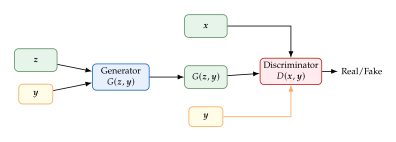
The vanilla GAN of Chapter 9 learns an unconditional generator $G : 𝒛 \mapsto 𝒙$ . In most practical settings we want to control the output: generate a face with a particular attribute, synthesise an image from a text caption, or translate a sketch into a photograph. Conditional GANs (cGANs) [4] achieve this by feeding auxiliary information $𝒚$ (a class label, an image, a text embedding, etc.) to both the generator and the discriminator.

The cGAN Objective

Definition 1 (Conditional GAN Objective).

Let $(𝒙, 𝒚) \sim p_{data} (𝒙, 𝒚)$ denote data–condition pairs and let $𝒛 \sim p_{𝒛} (𝒛)$ be a latent noise vector. The conditional GAN objective is (CGAN) $\begin{matrix} \min_{G} \max_{D} \underset{real pairs}{\underset{⏟}{𝔼_{(𝒙, 𝒚) \sim p_{data}} [\log D (𝒙, 𝒚)]}} + \underset{fake pairs}{\underset{⏟}{𝔼_{𝒛 \sim p_{𝒛}, 𝒚 \sim p (𝒚)} [\log (1 - D (G (𝒛, 𝒚), 𝒚))]}} . \end{matrix}$ The generator $G (𝒛, 𝒚)$ takes both noise and condition; the discriminator $D (𝒙, 𝒚)$ receives an image together with the condition and returns the probability that the pair is real.

Note the key structural difference from the unconditional GAN: the discriminator does not merely judge whether an image looks realistic; it judges whether the image is consistent with the given condition. A photorealistic cat image paired with the label “dog” should still be rejected.

Optimal Discriminator and Generator

The analysis parallels the unconditional case (Chapter 9), but all densities are now conditioned on $𝒚$ .

Proposition 1 (Optimal cGAN Discriminator).

For a fixed generator $G$ , the optimal discriminator is (Dstar) $\begin{matrix} D^{*} (𝒙, 𝒚) = \frac{p_{data} (𝒙 | 𝒚)}{p_{data} (𝒙 | 𝒚) + p_{G} (𝒙 | 𝒚)}, \end{matrix}$ where $p_{G} (𝒙 | 𝒚)$ is the conditional density induced by $G (𝒛, 𝒚)$ .

Proof.

For each fixed $(𝒙, 𝒚)$ , the integrand of the value function is $V (D; 𝒙, 𝒚) = p_{data} (𝒙 | 𝒚) \log D (𝒙, 𝒚) + p_{G} (𝒙 | 𝒚) \log (1 - D (𝒙, 𝒚)) .$ This is the same $a \log t + b \log (1 - t)$ form as in the unconditional derivation (see Proposition Proposition 1 in Chapter 9). Maximising over $t = D (𝒙, 𝒚) \in [0,1]$ by setting the derivative to zero gives $\frac{a}{t} - \frac{b}{1 - t} = 0 ⟹ t^{*} = \frac{a}{a + b} = \frac{p_{data} (𝒙 | 𝒚)}{p_{data} (𝒙 | 𝒚) + p_{G} (𝒙 | 𝒚)} .$

∎

Proposition 2 (cGAN Generator Minimises Conditional JSD).

Substituting $D^{*}$ back into the value function and minimising over $G$ yields (JSD) $\begin{matrix} \min_{G} 𝔼_{𝒚 \sim p (𝒚)} [2 𝖣_{JS} (p_{data} (\cdot | 𝒚) ‖ p_{G} (\cdot | 𝒚))] - \log 4, \end{matrix}$ so the generator minimises the expected conditional Jensen–Shannon divergence over the marginal distribution of conditions.

Proof.

Substituting into the value function and proceeding exactly as in the unconditional proof (Theorem Theorem 1 in Chapter 9), but with every density conditioned on $𝒚$ , gives $\begin{matrix} V (G, D^{*}) & = 𝔼_{𝒚} [\int p_{data} (𝒙 | 𝒚) \log \frac{p_{data} (𝒙 | 𝒚)}{p_{data} (𝒙 | 𝒚) + p_{G} (𝒙 | 𝒚)} d 𝒙 \\ + \int p_{G} (𝒙 | 𝒚) \log \frac{p_{G} (𝒙 | 𝒚)}{p_{data} (𝒙 | 𝒚) + p_{G} (𝒙 | 𝒚)} d 𝒙] \\ = 𝔼_{𝒚} [2 𝖣_{JS} (p_{data} (\cdot | 𝒚) ‖ p_{G} (\cdot | 𝒚))] - \log 4. \end{matrix}$ Since $𝖣_{JS} \geq 0$ with equality iff $p_{G} (\cdot | 𝒚) = p_{data} (\cdot | 𝒚)$ a.e., the global minimum is $- \log 4$ , attained when the generator perfectly matches the class-conditional data distribution for every $𝒚$ .

∎

Example 1 (Class-Conditional MNIST).

Consider generating handwritten digits $𝒙 \in {[0,1]}^{28 \times 28}$ conditioned on a digit label $y \in {0, 1, \dots, 9}$ . The condition $y$ is represented as a one-hot vector $𝒚 \in {0,1}^{10}$ . In the generator, $𝒚$ is concatenated with the noise vector $𝒛 \in ℝ^{100}$ before the first fully-connected layer; in the discriminator, $𝒚$ is concatenated with the flattened image. After training, fixing $y = 3$ and varying $𝒛$ produces diverse images of the digit “3”, while fixing $𝒛$ and varying $y$ produces the same style rendered as different digits, demonstrating that $𝒛$ controls style and $𝒚$ controls content.

Conditional GAN architecture. The generator receives both noise

𝒛

and condition

𝒚

. The discriminator judges whether an image–condition pair

(𝒙, 𝒚)

is real, enforcing not just realism but also consistency with the condition.

Key Idea.

Conditioning transforms an unconditional density model $p_{G} (𝒙)$ into a family of conditional models ${p_{G} (𝒙 | 𝒚)}_{𝒚}$ . The discriminator ensures that each conditional distribution is realistic and consistent with $𝒚$ ; without seeing $𝒚$ , it could only enforce marginal realism and the generator could ignore the condition entirely.

Paired Image-to-Image Translation: Pix2Pix

When the condition $𝒚$ is itself an image (a sketch, a segmentation map, or a low-resolution photograph) the cGAN framework becomes an image-to-image translation engine. Pix2Pix [5] instantiates this idea with two key design choices: an $ℓ_{1}$ reconstruction loss to encourage pixel-level fidelity, and a PatchGAN discriminator to enforce local texture realism.

The Pix2Pix Objective

Definition 2 (Pix2Pix Loss).

Given paired training data ${(𝒙_{i}, 𝒚_{i})}_{i = 1}^{N}$ where $𝒙_{i}$ is the target image and $𝒚_{i}$ is the input (condition) image, the Pix2Pix objective is (Pix2pix) $\begin{matrix} \min_{G} \max_{D} \underset{adversarial}{\underset{⏟}{ℒ_{cGAN} (G, D)}} + λ \underset{reconstruction}{\underset{⏟}{𝔼_{(𝒙, 𝒚)} [{‖ G (𝒚) - 𝒙 ‖}_{1}]}}, \end{matrix}$ where $ℒ_{cGAN}$ is the conditional GAN loss (without noise $𝒛$ , since the input image $𝒚$ provides all the stochasticity), and $λ > 0$ controls the reconstruction–realism trade-off.

Remark 1 (Why $ℓ_{1}$ Instead of $ℓ_{2}$ ?).

Minimising $𝔼 [{‖ G (𝒚) - 𝒙 ‖}_{2}^{2}]$ over $G$ yields the posterior mean $G^{*} (𝒚) = 𝔼 [𝒙 | 𝒚]$ , which averages over all plausible outputs and produces blurry results (recall the MMSE estimator from Theorem Theorem 1 in Chapter 12).

Minimising $𝔼 [{‖ G (𝒚) - 𝒙 ‖}_{1}]$ instead yields the posterior median, which is sharper because the $ℓ_{1}$ loss corresponds to a Laplace likelihood rather than a Gaussian one: $ℓ_{2} : p (𝒙 | G (𝒚)) \propto \exp (- \frac{1}{2 σ^{2}} {‖ 𝒙 - G (𝒚) ‖}_{2}^{2}) vs. ℓ_{1} : p (𝒙 | G (𝒚)) \propto \exp (- \frac{1}{b} {‖ 𝒙 - G (𝒚) ‖}_{1}) .$ The heavier tails of the Laplace distribution are more tolerant of sharp edges and outlier pixels, producing less blurring in practice.

The PatchGAN Discriminator

Definition 3 (PatchGAN Discriminator).

Instead of producing a single real/fake scalar for the entire image, the PatchGAN discriminator outputs a matrix $D (𝒙, 𝒚) \in {[0,1]}^{M \times M}$ , where entry $(i, j)$ classifies whether the $N \times N$ receptive-field patch centred at spatial location $(i, j)$ is real or fake. The adversarial loss becomes (Patchgan) $\begin{matrix} ℒ_{PatchGAN} = \frac{1}{M^{2}} \sum_{i, j} [\log D (𝒙, 𝒚)_{i j} + \log (1 - D (G (𝒚), 𝒚)_{i j})] . \end{matrix}$

Proposition 3 (PatchGAN as a Texture Loss).

Each element of the PatchGAN output depends only on the pixels within its $N \times N$ receptive field. Consequently, the PatchGAN loss penalises the generator for producing unrealistic local texture within each patch, effectively acting as a learned texture/style discriminator. If $N$ equals the full image size, PatchGAN reduces to a standard (global) discriminator; if $N = 1$ , it reduces to a per-pixel classifier (PixelGAN).

Proof.

Consider the discriminator as a fully convolutional network with effective receptive field of side length $N$ . Each layer with kernel size $k_{l}$ and stride $s_{l}$ updates the receptive field $r$ and the jump $j$ by $r \leftarrow r + (k_{l} - 1) j$ and $j \leftarrow j s_{l}$ , starting from $r = j = 1$ . For $k$ layers of $4 \times 4$ convolutions with stride $2$ this gives $N = 1 + 3 \sum_{l = 0}^{k - 1} 2^{l} = 3 \cdot 2^{k} - 2,$ so $N = 4, 10, 22, 46$ for $k = 1,2,3,4$ . Each output unit $D {(𝒙, 𝒚)}_{i j}$ is a function only of the $N \times N$ sub-image centred at $(i, j)$ . The per-patch losses are then independent classification problems: each enforces realism within its own local region. Summing over all patches and dividing by $M^{2}$ yields an average over all overlapping patches, equivalent to encouraging realistic local statistics everywhere, i.e., a learned texture loss.

∎

Example 2 (Receptive Field Calculation).

The Pix2Pix “ $70 \times 70$ ” PatchGAN (the n_layers $= 3$ configuration) uses $4 \times 4$ convolutions throughout: three stride- $2$ layers, then a stride- $1$ layer, then the stride- $1$ output convolution. Writing $r$ for the receptive field and $j$ for the jump (the input-pixel spacing between adjacent units), each layer applies $r \leftarrow r + (k - 1) j$ and then $j \leftarrow j \cdot s$ :

Layer	Kernel	Jump in	Receptive field
Input	-	$1$	$1 \times 1$
Conv1 (stride 2)	$4 \times 4$	$1$	$4 \times 4$
Conv2 (stride 2)	$4 \times 4$	$2$	$10 \times 10$
Conv3 (stride 2)	$4 \times 4$	$4$	$22 \times 22$
Conv4 (stride 1)	$4 \times 4$	$8$	$46 \times 46$
Output (stride 1)	$4 \times 4$	$8$	$70 \times 70$

The stride-

1

penultimate layer is easy to overlook, but it is what carries the receptive field from

46

70

: after three stride-

2

layers the jump is already

8

, so each further

4 \times 4

convolution adds

3 \times 8 = 24

input pixels. Stopping at Conv3 would give a

46 \times 46

patch, not

70 \times 70

. This

70 \times 70

PatchGAN is the default in the original Pix2Pix paper and strikes a good balance: large enough to capture texture patterns (brick walls, grass, sky), small enough to avoid penalising global structure (which the

ℓ_{1}

loss already handles).

Insight.

Pix2Pix has the same two-part shape as a MAP estimate: a fidelity term plus a prior term. By Remark Remark 1 the $ℓ_{1}$ reconstruction loss is the negative log-likelihood of a Laplace observation model for the target given the prediction, $- \log p (𝒙 | G (𝒚))$ , while the adversarial loss acts as a learned log-prior $\log p (𝒙)$ : the discriminator scores how plausible an image is, which is exactly the job a hand-crafted regulariser performs in classical MAP estimation (Chapter 12). The generator is therefore pushed towards outputs that are both faithful to the paired target and “look real” according to the discriminator.

The correspondence is structural rather than literal: the $ℓ_{1}$ term is a supervised loss against a known ground-truth target, not a forward-model likelihood evaluated at test time. What carries over from Chapter 12 is the division of labour, with one term enforcing agreement with the data and the other enforcing plausibility, and the fact that the second term is now learned rather than hand-designed.

Unpaired Translation: CycleGAN

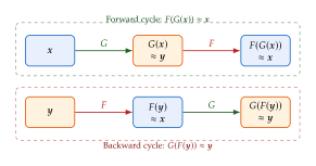
Pix2Pix requires paired examples: for every input sketch there must be a corresponding target photograph. In many settings such pairs are unavailable; we may have a collection of photographs and a collection of Monet paintings, but no “Monet version” of each photograph. CycleGAN [6] tackles this unpaired setting by introducing a cycle-consistency constraint.

Problem Setup

Let $𝒳$ and $𝒴$ be two image domains with marginal distributions $p_{𝒳}$ and $p_{𝒴}$ . We seek two mappings: $G : 𝒳 \to 𝒴, F : 𝒴 \to 𝒳,$ such that $G (𝒙)$ looks like a sample from $𝒴$ and $F (𝒚)$ looks like a sample from $𝒳$ , while the semantic content is preserved.

The CycleGAN Objective

Definition 4 (CycleGAN Loss).

The full CycleGAN objective combines two adversarial losses with a cycle-consistency loss: (Cyclegan) $\begin{matrix} ℒ (G, F, D_{𝒳}, D_{𝒴}) = ℒ_{GAN} (G, D_{𝒴}) + ℒ_{GAN} (F, D_{𝒳}) + λ ℒ_{cyc} (G, F), \end{matrix}$ where the adversarial losses are (ADV1) $\begin{matrix} ℒ_{GAN} (G, D_{𝒴}) & = 𝔼_{𝒚} [\log D_{𝒴} (𝒚)] + 𝔼_{𝒙} [\log (1 - D_{𝒴} (G (𝒙)))], \\ ℒ_{GAN} (F, D_{𝒳}) & = 𝔼_{𝒙} [\log D_{𝒳} (𝒙)] + 𝔼_{𝒚} [\log (1 - D_{𝒳} (F (𝒚)))], \end{matrix}$ and the cycle-consistency loss is (CYC) $\begin{matrix} ℒ_{cyc} (G, F) = \underset{forward cycle}{\underset{⏟}{𝔼_{𝒙} [{‖ F (G (𝒙)) - 𝒙 ‖}_{1}]}} + \underset{backward cycle}{\underset{⏟}{𝔼_{𝒚} [{‖ G (F (𝒚)) - 𝒚 ‖}_{1}]}} . \end{matrix}$

CycleGAN enforces two cycle-consistency constraints. Forward cycle: translate

𝒙

to domain

𝒴

via

G

, then back via

F

; the result should recover

𝒙

. Backward cycle: translate

𝒚

𝒳

via

F

, then back via

G

; the result should recover

𝒚

Why Cycle-Consistency Works

Without the cycle-consistency loss, each generator could learn an arbitrary mapping that produces realistic outputs but bears no semantic relationship to the input (e.g., mapping every horse photograph to the same zebra). The cycle constraint prevents this by forcing the mappings to be approximately invertible.

Theorem 1 (Cycle-Consistency Implies Approximate Inverse).

Let $G : 𝒳 \to 𝒴$ and $F : 𝒴 \to 𝒳$ be deterministic, measurable mappings. If $F (G (𝒙)) = 𝒙 for p_{𝒳} -a.e. 𝒙, G (F (𝒚)) = 𝒚 for p_{𝒴} -a.e. 𝒚,$ then $G$ is a bijection between $supp (p_{𝒳})$ and $supp (p_{𝒴})$ , and $F = G^{- 1}$ $p_{𝒴}$ -almost everywhere.

Proof.

The forward cycle condition $F \circ G = id$ on $supp (p_{𝒳})$ implies that $G$ is injective on $supp (p_{𝒳})$ (distinct inputs cannot map to the same output, since $F$ would then recover both).

The backward cycle condition $G \circ F = id$ on $supp (p_{𝒴})$ implies that $G$ is surjective onto $supp (p_{𝒴})$ (every $𝒚$ in the support is the image of $F (𝒚)$ under $G$ ).

Injectivity and surjectivity together give bijectivity. From $F \circ G = id$ , we have $F = G^{- 1}$ on $range (G) \supseteq supp (p_{𝒴})$ .

∎

Remark 2 (Identity Loss).

In practice, an identity loss is added: $ℒ_{idt} = 𝔼_{𝒚} [{‖ G (𝒚) - 𝒚 ‖}_{1}] + 𝔼_{𝒙} [{‖ F (𝒙) - 𝒙 ‖}_{1}] .$ This encourages $G$ to act as an identity when applied to an image already in the target domain, preventing unnecessary colour shifts (e.g., when translating Monet $\to$ photographs, a photograph should remain unchanged).

Caution.

CycleGAN assumes that the mapping between domains preserves geometric structure: a horse's outline should map to a zebra's outline. When this assumption fails, for example when translating between domains with different geometry (cats $\to$ dogs), CycleGAN can produce artefacts or hallucinate structures. The cycle-consistency loss cannot prevent semantic errors, only reconstruction errors.

Progressive Growing of GANs

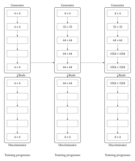
Generating high-resolution images (e.g., $1024 \times 1024$ ) directly is extremely difficult: the generator must simultaneously learn coarse structure (object layout) and fine detail (skin pores, hair strands), and the discriminator must evaluate both global coherence and local texture. Progressive Growing of GANs (ProGAN) [1] addresses this by training the networks in a curriculum: start at very low resolution and gradually add layers that handle finer details.

The Progressive Training Strategy

Definition 5 (Progressive Training Schedule).

Let $G_{k}$ and $D_{k}$ denote the generator and discriminator at resolution stage $k$ , where stage $k$ operates at resolution $r_{k} = 4 \cdot 2^{k}$ (so $k = 0$ is $4 \times 4$ , $k = 1$ is $8 \times 8$ , etc.). Training proceeds as follows:

Train $(G_{0}, D_{0})$ at $4 \times 4$ until convergence.
For $k = 1, 2, \dots, K$ : enumerate
Add new layers to both $G_{k - 1}$ and $D_{k - 1}$ to handle resolution $r_{k}$ .
Fade in the new layers using a blending parameter $α \in [0,1]$ that linearly increases from $0$ to $1$ over a fixed number of iterations.
Continue training at resolution $r_{k}$ . enumerate

The Fade-In Mechanism

Definition 6 (Fade-In Blending).

When transitioning from resolution $r_{k - 1}$ to $r_{k}$ , the generator output is computed as (Fadein) $\begin{matrix} {\hat{𝒙}}_{r_{k}} = (1 - α) \cdot Upsample ({\hat{𝒙}}_{r_{k - 1}}) + α \cdot NewBlock (𝒇_{r_{k}}), \end{matrix}$ where ${\hat{𝒙}}_{r_{k - 1}}$ is the previous-resolution output, $Upsample$ is nearest-neighbour upsampling followed by a $1 \times 1$ convolution (the “toRGB” layer from the old block), $𝒇_{r_{k}}$ is the feature map from the new convolutional block, and $NewBlock$ includes the new toRGB layer. The blending parameter $α$ increases linearly from $0$ to $1$ during the transition phase.

An analogous fade-in is applied in the discriminator, where a $1 \times 1$ “fromRGB” convolution is blended with the output of the new higher-resolution processing block.

Proposition 4 (Smooth Transition Preserves Training Stability).

At $α = 0$ , the output ${\hat{𝒙}}_{r_{k}} = Upsample ({\hat{𝒙}}_{r_{k - 1}})$ is identical to the old-resolution output (upsampled), so the generator's distribution is unchanged. At $α = 1$ , the old path is fully replaced by the new block. For intermediate $α$ , the output is a convex combination, so the distributional change is continuous. This prevents the “shock” that would occur if new randomly-initialised layers were suddenly activated.

Proof.

Let $p_{α}$ denote the generator's output distribution at blending parameter $α$ . Since is a convex combination of two continuous functions of the parameters, the mapping $α \mapsto {\hat{𝒙}}_{r_{k}}$ is continuous. By the continuous mapping theorem, $α \mapsto p_{α}$ is continuous in the weak topology on probability measures. In particular, $p_{0} = p_{r_{k - 1}}^{↑}$ (the upsampled old distribution), ensuring no discontinuity at the transition boundary.

∎

Progressive growing of GANs. Training begins at

4 \times 4

resolution (left) and progressively adds layers to reach

1024 \times 1024

(right).

G

denotes generator blocks and

D

denotes discriminator blocks. At each transition, new layers are faded in smoothly via .

Remark 3 (Minibatch Standard Deviation).

To encourage the generator to produce diverse outputs, ProGAN appends a minibatch standard deviation layer near the end of the discriminator. For a minibatch ${𝒙_{1}, \dots, 𝒙_{B}}$ , compute $σ = \sqrt{\frac{1}{B} \sum_{i = 1}^{B} {(𝒙_{i} - \overline{𝒙})}^{2} + ϵ}$ (element-wise, then averaged over all dimensions to produce a single scalar), replicate it as a constant feature map, and concatenate it with the final discriminator features. If the generator produces identical images (mode collapse), $σ \approx 0$ , giving the discriminator an easy signal to reject the batch.

Historical Note.

ProGAN [1] was the first GAN to produce photorealistic face images at $1024 \times 1024$ resolution. It also introduced the CelebA-HQ dataset, a high-quality version of CelebA that became a standard benchmark. The progressive training idea directly inspired StyleGAN (Style-Based Generation: StyleGAN), which inherits the progressive architecture but adds a style-based generator for finer control.

Style-Based Generation: StyleGAN

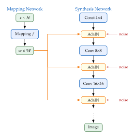
StyleGAN [7] builds on ProGAN's progressive architecture but fundamentally redesigns the generator. Instead of feeding the latent code $𝒛$ directly into the first layer, StyleGAN introduces a mapping network and injects style information at every resolution level through adaptive instance normalisation (AdaIN).

The Mapping Network

Definition 7 (Mapping Network).

The mapping network is a multilayer perceptron $f : 𝒵 \to 𝒲$ that transforms the latent code $𝒛 \sim Normal (0, I)$ to an intermediate latent code $𝒘 = f (𝒛) \in 𝒲$ . In the original StyleGAN, $f$ consists of 8 fully-connected layers with LeakyReLU activations, and $\dim (𝒵) = \dim (𝒲) = 512$ .

Proposition 5 (Disentanglement via the Mapping Network).

The latent space $𝒵$ is typically a hypersphere or Gaussian, which is a fixed geometry. The factors of variation in natural images (pose, lighting, expression, hair colour, etc.) do not respect this geometry: certain combinations may be impossible (e.g., a baby with wrinkles). A direct mapping $𝒛 \mapsto 𝒙$ must “warp” the latent space to avoid these forbidden regions, leading to entangled representations.

The mapping network $f$ learns a nonlinear warping $𝒛 \mapsto 𝒘$ such that $𝒲$ is adapted to the data manifold. Forbidden regions in $𝒵$ are mapped away, and the resulting $𝒲$ space has a geometry where linear interpolation corresponds to semantically meaningful changes.

Adaptive Instance Normalisation

Definition 8 (Adaptive Instance Normalisation (AdaIN)).

Let $𝒇_{i} \in ℝ^{H \times W}$ be the $i$ -th feature map in a convolutional layer and let $𝒘 \in 𝒲$ be the style code. A learned affine transformation $A$ maps $𝒘$ to per-channel scale and bias: (Affine) $\begin{matrix} (y_{s, i}, y_{b, i}) = A_{i} (𝒘), i = 1, \dots, C, \end{matrix}$ where $C$ is the number of channels. AdaIN then normalises and re-scales each feature map: (Adain) $\begin{matrix} AdaIN (𝒇_{i}, 𝒘) = y_{s, i} \frac{𝒇_{i} - μ (𝒇_{i})}{σ (𝒇_{i}) + ϵ} + y_{b, i}, \end{matrix}$ where $μ (𝒇_{i})$ and $σ (𝒇_{i})$ are the spatial mean and standard deviation of $𝒇_{i}$ (computed over $H \times W$ ), and $ϵ > 0$ is a small constant for numerical stability.

Remark 4 (AdaIN as Style Injection).

Instance normalisation removes the original feature statistics (mean and variance), which encode “style” information such as contrast, colour palette, and texture amplitude. AdaIN then replaces these statistics with new ones derived from $𝒘$ . Different layers control different aspects of the image:

Low-resolution layers ( $4 \times 4$ to $8 \times 8$ ): control coarse features such as pose, face shape, presence of accessories (glasses, hats).
Mid-resolution layers ( $16 \times 16$ to $32 \times 32$ ): control facial features, hairstyle, eyes open/closed.
High-resolution layers ( $64 \times 64$ to $1024 \times 1024$ ): control colour scheme, micro-structure, skin texture, background details.

Style Mixing

Definition 9 (Style Mixing Regularisation).

During training, two latent codes $𝒛_{1}, 𝒛_{2}$ are sampled and mapped to $𝒘_{1} = f (𝒛_{1})$ , $𝒘_{2} = f (𝒛_{2})$ . A random crossover point $k$ is chosen, and the generator uses $𝒘_{1}$ for layers $1, \dots, k$ and $𝒘_{2}$ for layers $k + 1, \dots, L$ . This prevents the network from assuming that adjacent layers are correlated, encouraging each layer to independently control its corresponding level of detail.

Example 3 (Style Mixing Matrix).

Consider two source latent codes $𝒘_{A}$ and $𝒘_{B}$ that produce face images $A$ and $B$ respectively. Injecting $𝒘_{A}$ at coarse layers and $𝒘_{B}$ at fine layers produces a face with the pose and structure of $A$ but the colour and texture of $B$ . Reversing the assignment gives $B$ 's structure with $A$ 's style. This decomposition is possible only because AdaIN applies style at each resolution independently.

The Truncation Trick

Definition 10 (Truncation Trick).

Let $\overline{𝒘} = 𝔼_{𝒛} [f (𝒛)]$ be the mean of the $𝒲$ distribution. The truncated style code is (Truncation) $\begin{matrix} 𝒘^{'} = \overline{𝒘} + ψ (𝒘 - \overline{𝒘}), \end{matrix}$ where $ψ \in [0, 1]$ is the truncation parameter. At $ψ = 1$ (no truncation), the full diversity of the model is used. At $ψ = 0$ , every image is the “average face” $G (\overline{𝒘})$ . Intermediate values trade diversity for quality.

Proposition 6 (Truncation as Variance Reduction).

If $𝒘 \sim 𝒩 (\overline{𝒘}, Σ)$ approximately (the distribution in $𝒲$ after passing through $f$ ), then $𝒘^{'}$ from satisfies $𝒘^{'} \sim 𝒩 (\overline{𝒘}, ψ^{2} Σ)$ . The variance is reduced by $ψ^{2}$ , concentrating samples near the mean of the learned manifold where the generator has seen the most training data and thus produces the highest quality.

Proof.

$𝒘^{'} - \overline{𝒘} = ψ (𝒘 - \overline{𝒘})$ . Since scaling a Gaussian by $ψ$ scales the covariance by $ψ^{2}$ : $𝖢ov (𝒘^{'}) = ψ^{2} 𝖢ov (𝒘) = ψ^{2} Σ .$

∎

StyleGAN generator architecture. The mapping network

f

transforms

𝒛

to the intermediate latent

𝒘

, which is injected at every resolution via AdaIN layers. Per-layer noise inputs add stochastic variation (e.g., freckles, hair placement). The synthesis network begins from a learned constant and progressively upsamples.

Insight.

StyleGAN's key insight is that style and content are best controlled at different resolutions. By injecting the latent code through AdaIN at every layer, rather than only at the input, StyleGAN gains fine-grained control: changing $𝒘$ at coarse layers alters pose and shape, while changing it at fine layers alters colour and micro-texture. This per-layer control is what makes style mixing and the truncation trick possible.

Semantic Image Synthesis: SPADE

In semantic image synthesis, the goal is to generate a photorealistic image from a semantic label map: a spatial map $𝒔 \in {1, \dots, K}^{H \times W}$ where each pixel is assigned a semantic class (sky, road, building, tree, etc.). GauGAN [8] solves this problem with Spatially-Adaptive Normalisation (SPADE), a normalisation layer that modulates features spatially based on the semantic layout.

Why BatchNorm Fails for Semantic Synthesis

Proposition 7 (BatchNorm Destroys Spatial Information).

Standard batch normalisation computes channel-wise statistics $μ_{c}, σ_{c}$ over the entire spatial extent and normalises: $BN (𝒉_{c, h, w}) = γ_{c} \frac{𝒉_{c, h, w} - μ_{c}}{σ_{c} + ϵ} + β_{c} .$ The affine parameters $γ_{c}, β_{c}$ are spatially uniform: the same scale and shift applied everywhere. When the input is a semantic map (encoded, e.g., as a one-hot volume), the normalisation step subtracts the global mean and divides by the global standard deviation, washing out the spatial layout of the semantic classes. After a few BN layers, the generator effectively loses the input segmentation map.

Spatially-Adaptive Normalisation

Definition 11 (SPADE Layer).

Let $𝒉 \in ℝ^{C \times H \times W}$ be the activation tensor at some generator layer and $𝒔 \in {1, \dots, K}^{H^{'} \times W^{'}}$ be the input semantic map (resized to $H \times W$ if needed). The SPADE layer computes: (Spade) $\begin{matrix} SPADE {(𝒉, 𝒔)}_{c, h, w} = γ_{c, h, w} (𝒔) \frac{𝒉_{c, h, w} - μ_{c}}{σ_{c} + ϵ} + β_{c, h, w} (𝒔), \end{matrix}$ where:

$μ_{c} = \frac{1}{H W} \sum_{h, w} 𝒉_{c, h, w}$ and $σ_{c}^{2} = \frac{1}{H W} \sum_{h, w} {(𝒉_{c, h, w} - μ_{c})}^{2}$ are the usual channel-wise statistics,
$γ (𝒔), β (𝒔) \in ℝ^{C \times H \times W}$ are spatially-varying modulation parameters produced by small convolutional networks applied to the semantic map $𝒔$ : (Modulation) $\begin{matrix} γ (𝒔) = {Conv}_{γ} (ReLU ({Conv}_{0} (𝒔))), β (𝒔) = {Conv}_{β} (ReLU ({Conv}_{0} (𝒔))), \end{matrix}$ sharing the first convolution ${Conv}_{0}$ and then branching into separate convolutions for $γ$ and $β$ .

The crucial difference from BatchNorm and AdaIN is that $γ$ and $β$ vary with spatial position $(h, w)$ , determined by the semantic label at that location. A pixel labelled “sky” receives different modulation parameters than a pixel labelled “road”, allowing the generator to synthesise appropriate textures in each region.

Theorem 2 (SPADE Generalises Conditional BatchNorm and AdaIN).

The following normalisation layers are special cases of SPADE:

Batch Normalisation: set $γ_{c, h, w} (𝒔) = γ_{c}$ and $β_{c, h, w} (𝒔) = β_{c}$ (spatially constant, independent of $𝒔$ ).
Conditional BatchNorm: set $γ_{c, h, w} (𝒔) = γ_{c} (y)$ and $β_{c, h, w} (𝒔) = β_{c} (y)$ where $y$ is a class label (spatially constant, dependent on a global condition).
AdaIN: set $γ_{c, h, w} (𝒔) = y_{s, c}$ and $β_{c, h, w} (𝒔) = y_{b, c}$ where $(y_{s, c}, y_{b, c})$ are derived from a style vector (spatially constant, per-channel modulation from a style code).

SPADE is strictly more expressive because the modulation parameters are functions of both the channel $c$ and the spatial location $(h, w)$ , through the semantic map $𝒔$ .

Proof.

In each case, we verify that the restricted parameter form satisfies :

Case 1 (BN): Let $γ_{c, h, w} = γ_{c}$ and $β_{c, h, w} = β_{c}$ for all $(h, w)$ . Then reduces to standard BN with learned affine parameters.

Case 2 (Conditional BN): Let $γ_{c, h, w} = γ_{c} (y)$ and $β_{c, h, w} = β_{c} (y)$ , where $y$ is a global class label. These are spatially constant but condition-dependent, matching Conditional BN.

Case 3 (AdaIN): Let $γ_{c, h, w} = y_{s, c} (𝒘)$ and $β_{c, h, w} = y_{b, c} (𝒘)$ , where $𝒘$ is a style vector. The normalisation uses instance statistics (per-example rather than per-batch), and the affine parameters depend on $𝒘$ but not on $(h, w)$ , recovering AdaIN .

In all three cases, $γ$ and $β$ are constrained to be spatially uniform. SPADE allows them to vary with $(h, w)$ through the semantic map, providing a strictly richer parameterisation.

∎

Example 4 (Cityscapes Synthesis).

The Cityscapes dataset [2] contains paired data: semantic label maps of urban scenes and corresponding photographs. Using SPADE, a generator trained on this data can take a new label map, perhaps user-drawn, and produce a photorealistic street scene. Moving a “tree” label to a different location in the map causes a tree to appear in the corresponding position in the generated image, demonstrating that SPADE truly respects the spatial layout. Evaluation on Cityscapes shows significant improvements in FID and segmentation accuracy over Pix2Pix and Pix2PixHD [3].

Insight.

The evolution of normalisation in GAN generators follows a clear trajectory of increasing expressiveness: $\underset{global}{\underset{⏟}{BN}} \to \underset{class-aware}{\underset{⏟}{Cond. BN}} \to \underset{style-aware}{\underset{⏟}{AdaIN}} \to \underset{spatially-aware}{\underset{⏟}{SPADE}} .$ Each step adds a new axis of modulation, giving the generator finer control over what it produces and where.

Scaling and the Bigger Picture

The architectures above were designed for resolutions up to $1024 \times 1024$ . Scaling GANs further, to text-conditioned generation at arbitrary resolutions, requires additional innovations.

GigaGAN

GigaGAN [9] scales GAN-based text-to-image synthesis to 512px base resolution with a 1-billion-parameter generator, rivalling diffusion models in quality while retaining the fast single-pass inference speed of GANs. Key innovations include:

Sample-adaptive kernel selection: convolutional kernels are dynamically chosen based on the text embedding, giving each text prompt a customised filter bank.
Interleaved attention and convolution: self-attention layers (for global coherence) alternate with convolution layers (for local texture), balancing computational cost and receptive field.
Multi-scale training: the generator produces images at multiple resolutions simultaneously, with separate discriminators at each scale.

Architecture Comparison

Method	Conditioning	Paired?	Max Res.	Key Innovation
cGAN	Label / image / text	Varies	Varies	Condition fed to $G$ and $D$
Pix2Pix	Input image	Yes	$256^{2}$	PatchGAN + $ℓ_{1}$ loss
CycleGAN	None (unpaired)	No	$256^{2}$	Cycle-consistency loss
ProGAN	None	N/A	$1024^{2}$	Progressive growing + fade-in
StyleGAN	None (+ truncation)	N/A	$1024^{2}$	Mapping net + AdaIN
SPADE	Semantic map	Yes	$512^{2}$	Spatially-adaptive norm
GigaGAN	Text embedding	N/A	$512^{2} +$	Adaptive kernels + attention

Remark 5 (GANs and Diffusion Models).

Since 2021, diffusion models have largely overtaken GANs for image generation benchmarks, offering better mode coverage and training stability. However, GANs retain key advantages: single-pass generation (no iterative denoising), real-time inference, and a mature toolkit for image editing (latent space interpolation, style mixing). Many modern systems combine both: a diffusion model for high-quality generation with a GAN-based refiner for speed.

Key Idea.

Every GAN architecture in this chapter injects structure through one of four mechanisms:

Conditioning: cGAN, Pix2Pix, GigaGAN feed side information to guide generation.
Cycle-consistency: CycleGAN constrains two mappings to invert each other, supplying the structure that paired data would otherwise provide.
Normalisation: StyleGAN (AdaIN) and SPADE modulate feature statistics to control style and spatial layout.
Curriculum: ProGAN trains progressively from low to high resolution.

Understanding which mechanism a new architecture uses is the fastest way to categorise it and predict its strengths and limitations.

Exercises

Exercise 1 (Optimal cGAN Discriminator).

Derive the optimal discriminator $D^{*} (𝒙, 𝒚)$ for the conditional GAN objective from first principles. Show that substituting $D^{*}$ into the value function gives $V (G, D^{*}) = 𝔼_{𝒚} [2 𝖣_{JS} (p_{data} (\cdot | 𝒚) ‖ p_{G} (\cdot | 𝒚))] - \log 4.$ Under what condition does the global optimum $V^{*} = - \log 4$ hold?

Exercise 2 ( $ℓ_{1}$ vs. $ℓ_{2}$ Reconstruction).

Consider a 1D pixel $x$ with posterior distribution $p (x | y) = \frac{1}{2} δ (x - a) + \frac{1}{2} δ (x - b)$ for $a \neq b$ . Compute:

The minimiser of $𝔼 [| x - g |]$ (posterior median).
The minimiser of $𝔼 [{(x - g)}^{2}]$ (posterior mean).
Explain why the $ℓ_{2}$ minimiser $(a + b) / 2$ produces a “blurry” result that is not a valid sample, while either $ℓ_{1}$ minimiser ( $a$ or $b$ ) is a valid sample.

Exercise 3 (PatchGAN Receptive Field).

A PatchGAN discriminator uses $L$ convolutional layers, each with kernel size $k$ and stride $s$ . Show that the receptive field $N_{L}$ at the output satisfies $N_{L} = 1 + \sum_{l = 1}^{L} (k - 1) \prod_{j = 1}^{l - 1} s_{j} .$ Verify this formula for the 3-layer architecture in Example Example 2 with $k = 4$ , $s = 2$ .

Exercise 4 (Cycle-Consistency and Bijectivity).

Give a concrete example of two mappings $G, F$ that satisfy the forward cycle $F (G (𝒙)) = 𝒙$ for all $𝒙$ but do not satisfy the backward cycle $G (F (𝒚)) = 𝒚$ for all $𝒚$ . What kind of mapping is $G$ in this case (injective, surjective, or bijective)? Why does CycleGAN need both cycles?

Exercise 5 (CycleGAN Mode Collapse).

Suppose $G$ maps every image in $𝒳$ to the same image $𝒚_{0} \in 𝒴$ . Show that the cycle-consistency loss $𝔼 [{‖ F (G (𝒙)) - 𝒙 ‖}_{1}]$ cannot be zero unless $F$ maps $𝒚_{0}$ to every $𝒙$ simultaneously (which is impossible for a deterministic function). Conclude that cycle-consistency prevents this form of mode collapse.

Exercise 6 (Progressive Fade-In Analysis).

Consider the fade-in formula . At the start of the transition ( $α = 0$ ), the new layers have random weights. Argue that the gradient of the training loss with respect to the new layer parameters is scaled by $α$ , so the new layers receive very small gradients initially. Why is this beneficial for training stability?

Exercise 7 (AdaIN Feature Statistics).

Let $𝒇 \in ℝ^{H \times W}$ be a feature map with mean $μ$ and standard deviation $σ$ . After applying $AdaIN (𝒇, 𝒘) = y_{s} \cdot \frac{𝒇 - μ}{σ} + y_{b}$ , show that the output has mean $y_{b}$ and standard deviation $| y_{s} |$ . Interpret: AdaIN replaces the feature statistics with the style-derived values $(y_{s}, y_{b})$ .

Exercise 8 (Mapping Network Disentanglement).

Consider a simple 2D example where $𝒛 = (z_{1}, z_{2}) \sim Normal (0, I)$ and the data manifold is an L-shaped region: ${(x_{1}, x_{2}) : 0 \leq x_{1} \leq 1, 0 \leq x_{2} \leq 1} ∖ {(x_{1}, x_{2}) : x_{1} > 0.5, x_{2} > 0.5}$ .

Explain why a linear mapping $𝒛 \mapsto 𝒙$ cannot map the Gaussian $𝒛$ onto this L-shaped region without “wasting” probability mass. Argue that a nonlinear mapping network can learn to warp the Gaussian to avoid the forbidden region, leading to better disentanglement.

Exercise 9 (Truncation and FID).

The truncation trick trades diversity for quality. Explain qualitatively why:

Decreasing $ψ$ improves the “quality” component of FID (generated samples are closer to real samples).
Decreasing $ψ$ worsens the “diversity” component of FID (the generated distribution has lower variance than the real distribution).
There exists an optimal $ψ^{*}$ that minimises FID.

Exercise 10 (SPADE vs. AdaIN).

Consider a $2 \times 2$ feature map $𝒉 \in ℝ^{1 \times 2 \times 2}$ with a semantic map $𝒔$ where the top row is “sky” and the bottom row is “grass”. Write out explicitly the output of:

AdaIN with parameters $(y_{s}, y_{b})$ derived from a global style vector.
SPADE with parameters $γ_{1,1}, γ_{1,2}, γ_{2,1}, γ_{2,2}$ and $β_{1,1}, β_{1,2}, β_{2,1}, β_{2,2}$ derived from $𝒔$ .

Explain why SPADE can produce different textures for sky and grass pixels while AdaIN cannot.

Exercise 11 (Conditional Mode Collapse).

In a conditional GAN, mode collapse can manifest as the generator producing the same output for all noise vectors $𝒛$ given a fixed condition $𝒚$ , while still producing diverse outputs across different conditions. Define the intra-class LPIPS score as $S (y) = 𝔼_{𝒛_{1}, 𝒛_{2}} [d_{LPIPS} (G (𝒛_{1}, y), G (𝒛_{2}, y))],$ where $d_{LPIPS}$ is the perceptual distance. Explain why $S (y) \approx 0$ indicates conditional mode collapse for class $y$ , and propose a training diagnostic based on monitoring $S (y)$ during training.

Exercise 12 (Unifying Framework).

Consider the general conditional generation framework $\min_{G} \max_{D} ℒ_{adv} (G, D) + λ ℒ_{recon} (G)$ . Show that:

Pix2Pix uses $ℒ_{recon} = 𝔼 [{‖ G (𝒚) - 𝒙 ‖}_{1}]$ with paired data.
CycleGAN replaces the single reconstruction loss with the cycle-consistency loss $ℒ_{cyc}$ , enabling unpaired training.
When $λ = 0$ , the framework reduces to the vanilla (conditional) GAN, which has no reconstruction guarantee.
When $λ \to \infty$ , the adversarial loss becomes irrelevant and the generator minimises reconstruction error alone, producing blurry outputs (the MMSE solution).

Conclude that $λ$ controls the reconstruction–realism trade-off, analogous to the PSNR–perceptual quality trade-off in Chapter 12.

References

Progressive Growing of GANs for Improved Quality, Stability, and Variation

Tero Karras, Timo Aila, Samuli Laine, Jaakko Lehtinen

International Conference on Learning Representations · 2018

BibTeX

@inproceedings{karras2018progressive,
  title={Progressive Growing of {GAN}s for Improved Quality, Stability, and Variation},
  author={Karras, Tero and Aila, Timo and Laine, Samuli and Lehtinen, Jaakko},
  booktitle={International Conference on Learning Representations},
  year={2018}
}

Conference paper

The Cityscapes Dataset for Semantic Urban Scene Understanding

Marius Cordts, Mohamed Omran, Sebastian Ramos, Timo Rehfeld, Markus Enzweiler, Rodrigo Benenson, Uwe Franke, Stefan Roth, et al.

Proc. of the IEEE Conference on Computer Vision and Pattern Recognition (CVPR) · 2016

BibTeX

@inproceedings{Cordts2016Cityscapes,
title={The Cityscapes Dataset for Semantic Urban Scene Understanding},
author={Cordts, Marius and Omran, Mohamed and Ramos, Sebastian and Rehfeld, Timo and Enzweiler, Markus and Benenson, Rodrigo and Franke, Uwe and Roth, Stefan and Schiele, Bernt},
booktitle={Proc. of the IEEE Conference on Computer Vision and Pattern Recognition (CVPR)},
year={2016}
}

Conference paper

High-Resolution Image Synthesis and Semantic Manipulation with Conditional GANs

Ting-Chun Wang, Ming-Yu Liu, Jun-Yan Zhu, Andrew Tao, Jan Kautz, Bryan Catanzaro

Proceedings of the IEEE/CVF Conference on Computer Vision and Pattern Recognition · 2018

BibTeX

@inproceedings{wang2018highresolution,
  title={High-Resolution Image Synthesis and Semantic Manipulation with Conditional {GAN}s},
  author={Wang, Ting-Chun and Liu, Ming-Yu and Zhu, Jun-Yan and Tao, Andrew and Kautz, Jan and Catanzaro, Bryan},
  booktitle={Proceedings of the IEEE/CVF Conference on Computer Vision and Pattern Recognition},
  year={2018}
}

Conference paper

Conditional Generative Adversarial Nets

Mehdi Mirza, Simon Osindero

arXiv:1411.1784 · 2014

BibTeX

@misc{mirza2014conditional,
      title={Conditional Generative Adversarial Nets}, 
      author={Mehdi Mirza and Simon Osindero},
      year={2014},
      eprint={1411.1784},
      archivePrefix={arXiv},
      primaryClass={cs.LG}
}

Reference

Image-to-image translation with conditional adversarial networks

Phillip Isola, Jun-Yan Zhu, Tinghui Zhou, Alexei A Efros

Proceedings of the IEEE conference on computer vision and pattern recognition, pp. 1125-1134 · 2017

BibTeX

@inproceedings{isola2017image,
  title={Image-to-image translation with conditional adversarial networks},
  author={Isola, Phillip and Zhu, Jun-Yan and Zhou, Tinghui and Efros, Alexei A},
  booktitle={Proceedings of the IEEE conference on computer vision and pattern recognition},
  pages={1125--1134},
  year={2017}
}

Conference paper

Unpaired Image-to-Image Translation Using Cycle-Consistent Adversarial Networks

Jun-Yan Zhu, Taesung Park, Phillip Isola, Alexei A. Efros

IEEE International Conference on Computer Vision, pp. 2223-2232 · 2017

BibTeX

@inproceedings{zhu2017unpaired,
    title = {Unpaired Image-to-Image Translation Using Cycle-Consistent Adversarial Networks},
    author = {Zhu, Jun-Yan and Park, Taesung and Isola, Phillip and Efros, Alexei A.},
    booktitle = {IEEE International Conference on Computer Vision},
    pages = {2223--2232},
    year = {2017}
}

Conference paper

A Style-Based Generator Architecture for Generative Adversarial Networks

Tero Karras, Samuli Laine, Timo Aila

Proceedings of the IEEE/CVF Conference on Computer Vision and Pattern Recognition, pp. 4401-4410 · 2019

BibTeX

@inproceedings{karras2019style,
  title={A Style-Based Generator Architecture for Generative Adversarial Networks},
  author={Karras, Tero and Laine, Samuli and Aila, Timo},
  booktitle={Proceedings of the IEEE/CVF Conference on Computer Vision and Pattern Recognition},
  pages={4401--4410},
  year={2019}
}

Conference paper

Semantic Image Synthesis with Spatially-Adaptive Normalization

Taesung Park, Ming-Yu Liu, Ting-Chun Wang, Jun-Yan Zhu

Proceedings of the IEEE/CVF Conference on Computer Vision and Pattern Recognition · 2019

BibTeX

@inproceedings{park2019semantic,
  title={Semantic Image Synthesis with Spatially-Adaptive Normalization},
  author={Park, Taesung and Liu, Ming-Yu and Wang, Ting-Chun and Zhu, Jun-Yan},
  booktitle={Proceedings of the IEEE/CVF Conference on Computer Vision and Pattern Recognition},
  year={2019}
}

Conference paper

Scaling up GANs for Text-to-Image Synthesis

Minguk Kang, Jun-Yan Zhu, Richard Zhang, Jaesik Park, Eli Shechtman, Sylvain Paris, Taesung Park

Proceedings of the IEEE/CVF Conference on Computer Vision and Pattern Recognition · 2023

BibTeX

@inproceedings{kang2023scaling,
  title={Scaling up {GAN}s for Text-to-Image Synthesis},
  author={Kang, Minguk and Zhu, Jun-Yan and Zhang, Richard and Park, Jaesik and Shechtman, Eli and Paris, Sylvain and Park, Taesung},
  booktitle={Proceedings of the IEEE/CVF Conference on Computer Vision and Pattern Recognition},
  year={2023}
}

Conference paper

← 12 Vision Problems as Inverse Problems 14 Optimal Transport and Sinkhorn Generative Modelling →