9 Generative Adversarial Networks

Every generative model we have studied so far (mixture models, the EM algorithm, variational inference) works by defining an explicit probability density $p_{θ} (𝒙)$ and maximising its likelihood. This chapter introduces a radically different idea: what if we could learn to generate realistic data without ever writing down a density?

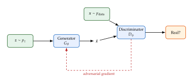
The generative adversarial network (GAN) achieves this by pitting two neural networks against each other in a game. A generator tries to produce fake data that looks real; a discriminator tries to tell fakes from real data. Through this adversarial competition, the generator learns to produce samples that are indistinguishable from the training data.

Key Idea.

The GAN is an implicit generative model: it defines a sampling procedure $𝒛 \mapsto G_{θ} (𝒛)$ but never computes $p_{θ} (𝒙)$ explicitly. This is both a strength (no intractable normalisation constant, no restrictive density assumptions) and a weakness (no likelihood for model comparison, harder to diagnose failure modes).

Historical Note.

Ian Goodfellow conceived the idea of GANs in June 2014 during a discussion with colleagues at a bar in Montréal [1]. The key insight, using a discriminator to provide a training signal for the generator, came from the realisation that the density ratio $p_{data} (𝒙) / p_{g} (𝒙)$ is all you need to measure how well the generator is doing, and a classifier naturally estimates this ratio. The paper was submitted, reviewed, and accepted at NeurIPS 2014 in a matter of months, a remarkable pace for what would become one of the most cited papers in machine learning. Within five years, GANs could generate photorealistic faces at $1024 \times 1024$ resolution [2].

The GAN Framework

Definition 1 (Generator and Discriminator).

A GAN consists of two neural networks:

The generator $G_{θ} : ℝ^{m} \to ℝ^{d}$ maps a latent code $𝒛 \sim p_{z} (𝒛)$ (typically $𝒩 (0, I)$ or $Uniform {[0,1]}^{m}$ ) to a synthetic data point $\hat{𝒙} = G_{θ} (𝒛)$ . The distribution of $\hat{𝒙}$ is called $p_{g}$ .
The discriminator $D_{ϕ} : ℝ^{d} \to [0, 1]$ takes a data point $𝒙$ and outputs the probability that $𝒙$ is real (from $p_{data}$ ) rather than fake (from $p_{g}$ ).

The GAN architecture. The generator

G_{θ}

maps latent noise

𝒛

to fake data

\hat{𝒙}

. The discriminator

D_{ϕ}

receives both real data

𝒙

and fakes, and outputs a probability of being real. The dashed arrow shows the adversarial gradient that trains the generator through the discriminator.

The Minimax Objective

The generator and discriminator play a two-player minimax game:

Definition 2 (GAN Value Function).

The GAN value function is (V) $\begin{matrix} V (G_{θ}, D_{ϕ}) = 𝔼_{𝒙 \sim p_{data}} [\log D_{ϕ} (𝒙)] + 𝔼_{𝒛 \sim p_{z}} [\log (1 - D_{ϕ} (G_{θ} (𝒛)))] . \end{matrix}$ The discriminator wants to maximise $V$ (correctly classify real and fake); the generator wants to minimise $V$ (fool the discriminator): (Minimax) $\begin{matrix} \min_{θ} \max_{ϕ} V (G_{θ}, D_{ϕ}) . \end{matrix}$

Example 1 (Reading the Objective).

When $D_{ϕ} (𝒙) \approx 1$ for real $𝒙$ : $\log D_{ϕ} (𝒙) \approx 0$ (good for $D$ ).
When $D_{ϕ} (G_{θ} (𝒛)) \approx 0$ (discriminator correctly rejects fakes): $\log (1 - D_{ϕ} (G_{θ} (𝒛))) \approx 0$ (good for $D$ , bad for $G$ ).
When $D_{ϕ} (G_{θ} (𝒛)) \approx 1$ (discriminator fooled): $\log (1 - D_{ϕ} (G_{θ} (𝒛))) \approx - \infty$ (bad for $D$ , good for $G$ , but $G$ minimises, so this is large negative $=$ good).

The objective perfectly balances the two players: what helps one hurts the other.

Remark 1 (Connection to Binary Cross-Entropy).

The value function is simply the negative binary cross-entropy of the discriminator, where real samples have label $y = 1$ and fake samples have label $y = 0$ . Training the discriminator to maximise $V$ is equivalent to training a binary classifier with cross-entropy loss.

Theoretical Analysis

The Optimal Discriminator

For a fixed generator, we can solve for the best possible discriminator in closed form.

Proposition 1 (Optimal Discriminator).

For a fixed generator $G$ with induced distribution $p_{g}$ , the discriminator that maximises $V (G, D)$ is (OPTD) $\begin{matrix} D_{G}^{*} (𝒙) = \frac{p_{data} (𝒙)}{p_{data} (𝒙) + p_{g} (𝒙)} . \end{matrix}$

Proof.

For fixed $G$ , we can write $V$ as an integral over $𝒙$ : $V (G, D) = \int_{𝒙} [p_{data} (𝒙) \log D (𝒙) + p_{g} (𝒙) \log (1 - D (𝒙))] d 𝒙 .$ We maximise the integrand pointwise. For any $𝒙$ , define $a = p_{data} (𝒙)$ and $b = p_{g} (𝒙)$ and consider $h (y) = a \log y + b \log (1 - y)$ for $y \in (0, 1)$ . Taking the derivative: $h^{'} (y) = \frac{a}{y} - \frac{b}{1 - y} = 0 ⟹ y^{*} = \frac{a}{a + b} .$ The second derivative $h^{''} (y) = - a / y^{2} - b / {(1 - y)}^{2} < 0$ confirms this is a maximum. Substituting back gives .

∎

Example 2 (Interpreting the Optimal Discriminator).

When $p_{data} (𝒙) = p_{g} (𝒙)$ (generator perfectly matches data), $D^{*} (𝒙) = 1 / 2$ everywhere, so the discriminator can do no better than random guessing. When $p_{g} (𝒙) = 0$ at some $𝒙$ where $p_{data} (𝒙) > 0$ (generator misses a mode), $D^{*} (𝒙) = 1$ there, and the discriminator is certain $𝒙$ is real.

Insight.

The optimal discriminator is a density ratio estimator: $D_{G}^{*} (𝒙) = \frac{p_{data} (𝒙)}{p_{data} (𝒙) + p_{g} (𝒙)} = σ (\log \frac{p_{data} (𝒙)}{p_{g} (𝒙)}),$ where $σ$ is the sigmoid function. This connects GANs to the broader idea of density ratio estimation, which appears throughout statistical machine learning.

The GAN Objective Equals the Jensen–Shannon Divergence

Theorem 1 (GAN Objective and JSD).

Substituting the optimal discriminator $D_{G}^{*}$ into the value function gives: (C) $\begin{matrix} C (G) \overset{def}{=} \max_{D} V (G, D) = - \log 4 + 2 \cdot 𝖣_{JS} (p_{data} ‖ p_{g}), \end{matrix}$ where $𝖣_{JS}$ is the Jensen–Shannon divergence (Definition Definition 5 in Chapter 4).

Proof.

Substituting into $V$ : $\begin{matrix} C (G) & = 𝔼_{p_{data}} [\log \frac{p_{data} (𝒙)}{p_{data} (𝒙) + p_{g} (𝒙)}] + 𝔼_{p_{g}} [\log \frac{p_{g} (𝒙)}{p_{data} (𝒙) + p_{g} (𝒙)}] . \end{matrix}$ Let $m = \frac{1}{2} (p_{data} + p_{g})$ . Then: $\begin{matrix} C (G) & = 𝔼_{p_{data}} [\log \frac{p_{data}}{2 m}] + 𝔼_{p_{g}} [\log \frac{p_{g}}{2 m}] \\ = - \log 4 + 𝖣_{KL} (p_{data} ‖ m) + 𝖣_{KL} (p_{g} ‖ m) \\ = - \log 4 + 2 𝖣_{JS} (p_{data} ‖ p_{g}) . \end{matrix}$

∎

Theorem 2 (Global Optimum of the GAN Game).

The global minimum of $C (G)$ is $- \log 4$ , achieved if and only if $p_{g} = p_{data}$ .

Proof.

Since $𝖣_{JS} (p_{data} ‖ p_{g}) \geq 0$ with equality iff $p_{data} = p_{g}$ , we have $C (G) \geq - \log 4$ with equality iff $p_{g} = p_{data}$ . At this equilibrium, $D^{*} (𝒙) = 1 / 2$ for all $𝒙$ .

∎

Remark 2 (Connection to Chapter 4).

The GAN game implicitly minimises the Jensen–Shannon divergence between $p_{data}$ and $p_{g}$ , one of the divergence measures studied in Chapter 4. Recall that $𝖣_{JS}$ is symmetric, bounded ( $0 \leq 𝖣_{JS} \leq \log 2$ ), and always defined (unlike the KL divergence, which can be infinite when supports don't match). However, as we saw in Chapter 4, when $p_{data}$ and $p_{g}$ have disjoint supports, $𝖣_{JS}$ saturates at $\log 2$ , a problem we will revisit when motivating the Wasserstein GAN in the next chapter.

The $f$ -GAN Perspective

The original GAN implicitly minimises the JSD. A natural question is: can we minimise any $f$ -divergence? The answer is yes, via the variational representation of $f$ -divergences.

Variational Lower Bound on $f$ -Divergences

Recall from Chapter 4 that the $f$ -divergence is $𝖣_{f} (p ‖ q) = \int q (𝒙) f (\frac{p (𝒙)}{q (𝒙)}) d 𝒙$ , where $f$ is convex with $f (1) = 0$ . The key tool is the Fenchel conjugate.

Definition 3 (Fenchel Conjugate).

The Fenchel conjugate of a convex function $f$ is (Fenchel) $\begin{matrix} f^{*} (t) = \sup_{u \in dom (f)} {t u - f (u)} . \end{matrix}$ Since $f$ is closed and convex, the biconjugate satisfies $f^{* *} = f$ , so $f (u) = \sup_{t} {t u - f^{*} (t)}$ .

Proposition 2 (Variational Representation of $f$ -Divergence).

For any $f$ -divergence: (VAR) $\begin{matrix} 𝖣_{f} (p ‖ q) = \sup_{T : 𝒳 \to ℝ} [𝔼_{𝒙 \sim p} [T (𝒙)] - 𝔼_{𝒙 \sim q} [f^{*} (T (𝒙))]] . \end{matrix}$

Proof.

Substituting $f (u) = \sup_{t} {t u - f^{*} (t)}$ into the definition of $𝖣_{f}$ : $\begin{matrix} 𝖣_{f} (p ‖ q) & = \int q (𝒙) \sup_{t} {t \frac{p (𝒙)}{q (𝒙)} - f^{*} (t)} d 𝒙 \\ = \int \sup_{t} {t p (𝒙) - f^{*} (t) q (𝒙)} d 𝒙 \\ \geq \sup_{T} \int [T (𝒙) p (𝒙) - f^{*} (T (𝒙)) q (𝒙)] d 𝒙, \end{matrix}$ where the inequality (swapping $\sup$ and $\int$ ) becomes an equality when $T$ is allowed to vary freely over all measurable functions. This gives .

∎

Insight.

Equation transforms a divergence computation (which requires knowing the density ratio $p / q$ ) into an optimisation problem (which only requires samples from $p$ and $q$ ). This is the mathematical engine that powers all GAN-like methods: the function $T$ is parameterised by a neural network (the “critic” or discriminator), and the optimisation is performed via stochastic gradient ascent.

From $f$ -Divergence to GAN Objectives

Different choices of $f$ yield different GAN variants. Nowozin et al. [9] systematised this in the f-GAN framework:

Definition 4 (f-GAN Objective).

Given a generator $G_{θ}$ with pushforward $p_{g}$ , the f-GAN training objective is (FGAN) $\begin{matrix} \min_{θ} \sup_{ϕ} [𝔼_{𝒙 \sim p_{data}} [T_{ϕ} (𝒙)] - 𝔼_{𝒛 \sim p_{z}} [f^{*} (T_{ϕ} (G_{θ} (𝒛)))]] . \end{matrix}$

Divergence	$f (u)$	$f^{*} (t)$	GAN Name
KL	$u \log u$	$e^{t - 1}$	KL-GAN
Reverse KL	$- \log u$	$- 1 - \log (- t)$	RKLGAN
Jensen–Shannon	$u \log u - (u + 1) \log \frac{u + 1}{2}$	$- \log (2 - e^{t})$	JS-GAN
GAN	$u \log u - (u + 1) \log (u + 1)$	$- \log (1 - e^{t})$	Original GAN
Pearson $χ^{2}$	${(u - 1)}^{2}$	$t^{2} / 4 + t$	$χ^{2}$ -GAN
Squared Hellinger	${(\sqrt{u} - 1)}^{2}$	$t / (1 - t)$	Hellinger GAN

f

-GAN variants: different convex functions

f

yield different divergences and GAN objectives.

Example 3 (Recovering the Original GAN).

Take the GAN generator function $f (u) = u \log u - (u + 1) \log (u + 1)$ from Table 1, whose conjugate is $f^{*} (t) = - \log (1 - e^{t})$ , together with the activation function $T_{ϕ} (𝒙) = \log D_{ϕ} (𝒙)$ (where $D_{ϕ} : 𝒳 \to (0,1)$ ). Then $\begin{matrix} f^{*} (T_{ϕ} (𝒙)) & = - \log (1 - e^{\log D_{ϕ} (𝒙)}) = - \log (1 - D_{ϕ} (𝒙)), \end{matrix}$ so the variational objective becomes $𝔼_{p_{data}} [\log D_{ϕ} (𝒙)] + 𝔼_{p_{g}} [\log (1 - D_{ϕ} (𝒙))]$ , which is exactly the original GAN objective . The closely related Jensen–Shannon row of Table 1 yields $- \log (2 - D_{ϕ} (𝒙))$ instead, giving the JS-GAN rather than the original formulation.

Training GANs in Practice

The Training Algorithm

Algorithm 1 (GAN Training via Alternating SGD).

Input: Dataset $𝒟$ , batch size $m$ , discriminator steps $k$ , learning rates $η_{D}, η_{G}$ .

for each training iteration:

Discriminator update (repeat $k$ times): itemize
Sample ${𝒙^{(1)}, \dots, 𝒙^{(m)}}$ from $𝒟$ and ${𝒛^{(1)}, \dots, 𝒛^{(m)}}$ from $p_{z}$ .
Update $ϕ$ by ascending: $\nabla_{ϕ} \frac{1}{m} \sum_{i = 1}^{m} [\log D_{ϕ} (𝒙^{(i)}) + \log (1 - D_{ϕ} (G_{θ} (𝒛^{(i)})))] .$ itemize
Generator update (once): itemize
Sample ${𝒛^{(1)}, \dots, 𝒛^{(m)}}$ from $p_{z}$ .
Update $θ$ by descending: $\nabla_{θ} \frac{1}{m} \sum_{i = 1}^{m} \log (1 - D_{ϕ} (G_{θ} (𝒛^{(i)}))) .$ itemize

Remark 3 (Choosing $k$ ).

The hyperparameter $k$ controls the discriminator-to-generator update ratio. Using $k = 1$ (one discriminator step per generator step) is the most common choice and keeps training balanced. Using $k$ too large risks overfitting the discriminator; using $k$ too small means the discriminator provides poor gradient signal. Goodfellow et al. [1] used $k = 1$ in their experiments.

The Non-Saturating Loss

Caution.

The minimax generator loss $\log (1 - D (G (𝒛)))$ suffers from vanishing gradients early in training. When the discriminator easily rejects fakes ( $D (G (𝒛)) \approx 0$ ), we have $\log (1 - D (G (𝒛))) \approx \log 1 = 0$ , so the gradient $\nabla_{θ} \log (1 - D (G (𝒛)))$ is near zero. The generator receives almost no learning signal precisely when it needs it most.

The practical fix is the non-saturating (NS) loss:

Definition 5 (Non-Saturating Generator Loss).

Instead of minimising $𝔼 [\log (1 - D (G (𝒛)))]$ , the generator maximises: (LOSS) $\begin{matrix} ℒ_{G}^{NS} = 𝔼_{𝒛 \sim p_{z}} [\log D_{ϕ} (G_{θ} (𝒛))] . \end{matrix}$

Example 4 (Why Non-Saturating Helps).

When $D (G (𝒛)) \approx 0$ (early training):

Saturating loss: $\log (1 - 0) = 0$ , flat, no gradient.
Non-saturating loss: $\log (0) \to - \infty$ , strong gradient pushing $G$ to increase $D (G (𝒛))$ .

When $D (G (𝒛)) \approx 0.5$ (equilibrium), both losses provide similar gradients. The NS loss simply provides stronger signal when the generator is far from equilibrium.

Remark 4 (What Divergence Does the NS Loss Minimise?).

Under the optimal discriminator, the NS generator loss corresponds to minimising: $𝖣_{KL} (p_{g} ‖ p_{data}) - 2 𝖣_{JS} (p_{data} ‖ p_{g}) + const .$ The reverse KL term $𝖣_{KL} (p_{g} ‖ p_{data})$ is mode-seeking: it penalises the generator for placing mass where $p_{data}$ is small, but does not penalise missing modes. This contributes to the mode collapse phenomenon (Section Mode Collapse and Failure Modes).

Practical Guidelines: The DCGAN Recipe

Radford et al. [3] identified a set of architectural guidelines that stabilise GAN training for images:

Guideline	Rationale
Replace pooling with strided convolutions	Learnable downsampling
Use batch normalisation in $G$ and $D$	Stabilises gradient flow
Remove fully connected layers	All-convolutional
ReLU in generator (except output: tanh)	Avoids saturation
LeakyReLU in discriminator	Gradient flow for negatives
Use Adam with $η = 0.0002$ , $β_{1} = 0.5$	Tuned for stability

DCGAN architectural guidelines [3].

Remark 5 (Spectral Normalisation).

A later influential technique is spectral normalisation [4], which constrains the Lipschitz constant of the discriminator by normalising each weight matrix by its largest singular value. This provides a more principled form of regularisation than batch norm and is now widely used.

Mode Collapse and Failure Modes

Despite their impressive results, GANs suffer from several well-known failure modes.

Mode Collapse

Definition 6 (Mode Collapse).

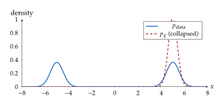
Mode collapse occurs when the generator maps all (or most) latent codes to a small region of data space, producing only a few types of outputs rather than the full diversity of the data distribution.

Example 5 (Mode Collapse in 1D).

Consider $p_{data} = \frac{1}{2} 𝒩 (- 5, 0.1) + \frac{1}{2} 𝒩 (5, 0.1)$ (two well-separated modes). If the generator parameterisation is $G (𝒛) = μ$ (a single learnable scalar, ignoring $𝒛$ ), then $p_{g} = δ_{μ}$ , a point mass. The generator can match one mode ( $μ \approx - 5$ or $μ \approx 5$ ) but never both.

Even with a more expressive generator, mode collapse can occur dynamically: the generator “chases” the discriminator's weak points, cycling between modes without ever covering all of them.

Mode collapse: the data distribution

p_{data}

(blue) has two modes, but the generator

p_{g}

(red dashed) concentrates all its mass on only one mode, completely missing the other.

Why GANs Are Hard to Train

Key Idea.

GAN training is a minimax (saddle-point) problem, not a minimisation problem. Standard gradient descent finds minima, but there is no guarantee it finds saddle points. This is the root cause of GAN training instability.

Example 6 (Failure of Simultaneous GD on a Bilinear Game).

Consider the simplest minimax game: $\min_{θ} \max_{ϕ} θ \cdot ϕ$ , with Nash equilibrium at $(θ^{*}, ϕ^{*}) = (0, 0)$ . Simultaneous gradient descent gives updates: $θ_{t + 1} = θ_{t} - η ϕ_{t}, ϕ_{t + 1} = ϕ_{t} + η θ_{t} .$ This is a rotation: $(θ_{t}, ϕ_{t})$ orbits the origin with increasing radius, diverging from the equilibrium! The eigenvalues of the update matrix $(\begin{matrix} 1 & - η \\ η & 1 \end{matrix})$ have magnitude $\sqrt{1 + η^{2}} > 1$ , confirming divergence.

The main failure modes in practice are:

Mode collapse (Section Mode Collapse): generator produces limited variety.
Training oscillation: generator and discriminator losses oscillate without converging.
Discriminator domination: $D$ becomes too strong too early, providing no useful gradient to $G$ .
Generator collapse: $G$ produces nonsensical outputs (noise, artefacts).

Remark 6 (Mitigation Strategies).

Numerous techniques have been proposed to stabilise GAN training:

Wasserstein distance instead of JSD (the next chapter).
Gradient penalty [5]: regularise the discriminator's gradient norm.
Spectral normalisation [4]: control the Lipschitz constant.
Progressive growing: start at low resolution and gradually increase.
Two-timescale updates: use different learning rates for $G$ and $D$ .

The Wasserstein GAN, discussed in the next chapter, addresses the most fundamental issue: the JSD's behaviour when supports are disjoint.

Evaluating GANs

Since GANs do not provide a tractable density $p_{θ} (𝒙)$ , we cannot evaluate them via log-likelihood. Several surrogate metrics have been developed.

Definition 7 (Fréchet Inception Distance (FID)).

The FID [6] compares the statistics of real and generated images in the feature space of a pretrained Inception network. Let $(𝝁_{r}, 𝚺_{r})$ and $(𝝁_{g}, 𝚺_{g})$ be the means and covariances of Inception features for real and generated images. Then: (FID) $\begin{matrix} FID = ‖ 𝝁_{r} - 𝝁_{g} ‖^{2} + trace (𝚺_{r} + 𝚺_{g} - 2 (𝚺_{r} 𝚺_{g})^{1 / 2}) . \end{matrix}$ Lower FID = better quality. FID $= 0$ iff the feature distributions are identical.

Remark 7 (FID Is a Wasserstein Distance).

The FID is exactly the squared $2$ -Wasserstein distance $W_{2}^{2}$ between two Gaussians fitted to the Inception features. This connects GAN evaluation to the optimal transport theory of Chapter 4.

Definition 8 (Inception Score (IS)).

The Inception Score [7] measures: (IS) $\begin{matrix} IS = \exp (𝔼_{𝒙 \sim p_{g}} [𝖣_{KL} (p (y | 𝒙) ‖ p (y))]), \end{matrix}$ where $p (y | 𝒙)$ is the Inception classifier's label distribution. Higher IS = samples are individually distinctive (low entropy $p (y | 𝒙)$ ) and collectively diverse (high entropy $p (y)$ ).

Caution.

Both FID and IS have significant limitations:

They depend on a pretrained Inception network (ImageNet features may not suit all domains).
IS does not compare to real data, only measures internal diversity.
Neither captures fine-grained artefacts that humans notice.
FID can be gamed by memorising training data.

Use multiple metrics and always include visual inspection when evaluating generative models.

Remark 8 (Precision and Recall for Generative Models).

Kynkäänniemi et al. proposed separating GAN quality into precision (are generated samples realistic?) and recall (does the generator cover all modes of the data?). A model with high precision but low recall exhibits mode collapse; a model with low precision but high recall produces diverse but poor-quality samples.

The GAN Landscape

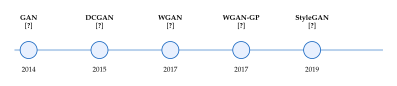
Since the original 2014 paper, GANs have evolved rapidly:

Key milestones in GAN development. Each addressed a fundamental limitation of its predecessor: DCGAN introduced convolutional architectures, WGAN replaced JSD with Wasserstein distance, WGAN-GP improved gradient penalty, and StyleGAN achieved photorealistic generation.

Remark 9 (Conditional GANs).

All the above GANs generate images unconditionally. Conditional GANs [8] augment both $G$ and $D$ with a conditioning variable $𝒚$ (e.g. a class label): $\min_{θ} \max_{ϕ} 𝔼_{(𝒙, 𝒚)} [\log D_{ϕ} (𝒙, 𝒚)] + 𝔼_{𝒛, 𝒚} [\log (1 - D_{ϕ} (G_{θ} (𝒛, 𝒚), 𝒚))] .$ This enables controllable generation: “generate a cat”, “generate a house with this floor plan”, etc. Conditional GANs underpin pix2pix (image-to-image translation) and many other applications discussed in later chapters.

Chapter Summary

A GAN consists of a generator $G_{θ}$ and discriminator $D_{ϕ}$ playing a minimax game.
The optimal discriminator is a density ratio estimator; substituting it into the objective reveals that GANs minimise the Jensen–Shannon divergence.
The $f$ -GAN framework generalises GANs to any $f$ -divergence via the Fenchel conjugate trick.
In practice, the non-saturating loss replaces the minimax generator loss to avoid vanishing gradients.
GANs suffer from mode collapse, training oscillation, and convergence difficulties inherent to minimax optimisation.
Evaluation relies on surrogate metrics (FID, IS) since GANs have no tractable likelihood.
The JSD's saturation when supports are disjoint motivates the Wasserstein GAN (next chapter).

Exercises

Exercise 1 (Optimal Discriminator Derivation).

For the GAN objective with fixed $G$ :

(a)
Show that the optimal discriminator is $D_{G}^{*} (𝒙) = p_{data} (𝒙) / (p_{data} (𝒙) + p_{g} (𝒙))$ .
(b)
Show that when $p_{data} = p_{g}$ , we have $D^{*} (𝒙) = 1 / 2$ for all $𝒙$ . Interpret this.
(c)
What happens to $D^{*} (𝒙)$ at a point $𝒙$ where $p_{g} (𝒙) = 0$ but $p_{data} (𝒙) > 0$ ?

Exercise 2 (GAN Objective and JSD).

After substituting $D_{G}^{*}$ into the objective, show that $C (G) = - \log 4 + 2 𝖣_{JS} (p_{data} ‖ p_{g})$ , and conclude $C (G) \geq - \log 4$ with equality iff $p_{g} = p_{data}$ .

Exercise 3 (Non-Saturating Loss Analysis).

(a)
Show that when $D (G (𝒛)) \approx 0$ , the gradient of the saturating loss $\log (1 - D (G (𝒛)))$ is near zero.
(b)
Show that the NS loss $- \log D (G (𝒛))$ has strong gradients in the same regime.
(c)
Show that under the optimal discriminator, the NS generator loss corresponds to minimising $𝖣_{KL} (p_{g} ‖ p_{data}) - 2 𝖣_{JS} (p_{data} ‖ p_{g}) + const$ .
(d)
Explain why the reverse KL term can lead to mode collapse.

Exercise 4 (Mode Collapse Scenario).

Let $p_{data} = \frac{1}{2} 𝒩 (- 5, 0.1) + \frac{1}{2} 𝒩 (5, 0.1)$ and $G (𝒛) = μ$ (constant).

(a)
Show the generator can never capture both modes.
(b)
Describe qualitatively how $μ$ evolves during training.
(c)
Suggest a generator architecture that can capture both modes.

Exercise 5 ( $f$ -Divergence Variants).

(a)
Show that $f (u) = u \log u$ gives the KL divergence. Compute its Fenchel conjugate $f^{*} (t) = e^{t - 1}$ .
(b)
Show that $f (u) = - \log u$ gives the reverse KL. Compute $f^{*}$ .
(c)
For the Pearson $χ^{2}$ divergence ( $f (u) = {(u - 1)}^{2}$ ), show that $f^{*} (t) = t^{2} / 4 + t$ .
(d)
Write the resulting GAN training objective for each case.

Exercise 6 (GAN Training Dynamics).

(a)
Explain why $k > 1$ discriminator steps per generator step can be beneficial. What happens if $k$ is too large?
(b)
If $D$ is optimal at every step, show $G$ minimises $2 𝖣_{JS} (p_{data} ‖ p_{g}) - \log 4$ .
(c)
For the bilinear game $V (θ, ϕ) = θ ϕ$ , show that simultaneous gradient descent diverges from the Nash equilibrium $(0, 0)$ .

Exercise 7 (FID Computation).

Suppose Inception features for real images have $𝝁_{r} = {(1, 0)}^{𝖳}$ , $𝚺_{r} = I$ , and for generated images $𝝁_{g} = {(2, 1)}^{𝖳}$ , $𝚺_{g} = 2 I$ .

(a)
Compute $‖ 𝝁_{r} - 𝝁_{g} ‖^{2}$ .
(b)
Compute ${(𝚺_{r} 𝚺_{g})}^{1 / 2}$ and the trace term in the FID formula.
(c)
What is the total FID?
(d)
How does FID change if we double all variances?

Exercise 8 (Density Ratio Interpretation).

(a)
Show that the optimal discriminator satisfies $\log \frac{D^{*} (𝒙)}{1 - D^{*} (𝒙)} = \log \frac{p_{data} (𝒙)}{p_{g} (𝒙)}$ .
(b)
Explain how this means training a discriminator is equivalent to estimating the log-density ratio.
(c)
If we had access to the exact density ratio, how could we compute the KL divergence $𝖣_{KL} (p_{data} ‖ p_{g})$ without knowing either density explicitly?

Exercise 9 (Comparing GAN and VAE).

(a)
List three advantages of GANs over VAEs.
(b)
List three advantages of VAEs over GANs.
(c)
A VAE generates blurry images; a GAN generates sharp but less diverse images. Explain this in terms of the divergences each model minimises (forward KL vs. reverse KL / JSD).
(d)
Can the two approaches be combined? Describe one hybrid model.

Exercise 10 (Conditional GAN Objective).

(a)
Write the minimax objective for a conditional GAN with class label $y$ .
(b)
Derive the optimal conditional discriminator $D^{*} (x, y)$ .
(c)
Show that the conditional GAN minimises $𝖣_{JS} (p_{data} (𝒙 | y) ‖ p_{g} (𝒙 | y))$ for each $y$ .

Exercise 11 (JSD Saturation and WGAN Motivation).

Let $p = 𝒩 (0, ϵ^{2})$ and $q = 𝒩 (μ, ϵ^{2})$ for small $ϵ > 0$ .

(a)
For what values of $μ / ϵ$ are $p$ and $q$ “essentially disjoint” (overlap $< 0.01$ )?
(b)
Show that when $p$ and $q$ are disjoint, $𝖣_{JS} (p ‖ q) = \log 2$ regardless of the distance between them.
(c)
In contrast, show that the Wasserstein distance $W_{1} (p, q) = | μ |$ varies smoothly with $μ$ .
(d)
Explain why this makes JSD unsuitable as a GAN training signal when $p_{data}$ and $p_{g}$ live on low-dimensional manifolds.

Exercise 12 (Inception Score from Scratch).

A toy “Inception classifier” has 3 classes and produces the following label distributions for 4 generated images:

Image	$P (y = 1 \| 𝒙)$	$P (y = 2 \| 𝒙)$	$P (y = 3 \| 𝒙)$
1	0.9	0.05	0.05
2	0.1	0.8	0.1
3	0.9	0.05	0.05
4	0.05	0.1	0.85

(a)
Compute the marginal $p (y) = \frac{1}{4} \sum_{i} p (y | 𝒙_{i})$ .
(b)
Compute $𝖣_{KL} (p (y | 𝒙_{i}) ‖ p (y))$ for each image.
(c)
Compute the Inception Score.
(d)
What IS would you get if all images had the same label distribution $(1 / 3, 1 / 3, 1 / 3)$ ? Explain why.

References

Generative Adversarial Networks

Ian Goodfellow, Jean Pouget-Abadie, Mehdi Mirza, Bing Xu, David Warde-Farley, Sherjil Ozair, Aaron Courville, Yoshua Bengio

Advances in Neural Information Processing Systems, vol. 27 · 2014

BibTeX

@inproceedings{goodfellow2014generative,
  title={Generative Adversarial Networks},
  author={Goodfellow, Ian and Pouget-Abadie, Jean and Mirza, Mehdi and Xu, Bing and Warde-Farley, David and Ozair, Sherjil and Courville, Aaron and Bengio, Yoshua},
  booktitle={Advances in Neural Information Processing Systems},
  volume={27},
  year={2014}
}

Conference paper

A Style-Based Generator Architecture for Generative Adversarial Networks

Tero Karras, Samuli Laine, Timo Aila

Proceedings of the IEEE/CVF Conference on Computer Vision and Pattern Recognition, pp. 4401-4410 · 2019

BibTeX

@inproceedings{karras2019style,
  title={A Style-Based Generator Architecture for Generative Adversarial Networks},
  author={Karras, Tero and Laine, Samuli and Aila, Timo},
  booktitle={Proceedings of the IEEE/CVF Conference on Computer Vision and Pattern Recognition},
  pages={4401--4410},
  year={2019}
}

Conference paper

Unsupervised Representation Learning with Deep Convolutional Generative Adversarial Networks

Alec Radford, Luke Metz, Soumith Chintala

International Conference on Learning Representations · 2016

BibTeX

@inproceedings{radford2015unsupervised,
  title={Unsupervised Representation Learning with Deep Convolutional Generative Adversarial Networks},
  author={Radford, Alec and Metz, Luke and Chintala, Soumith},
  booktitle={International Conference on Learning Representations},
  year={2016}
}

Conference paper

Spectral normalization for generative adversarial networks

Takeru Miyato, Toshiki Kataoka, Masanori Koyama, Yuichi Yoshida

Proceedings of the International Conference on Learning Representations · 2018

BibTeX

@inproceedings{miyato2018spectral,
  title={Spectral normalization for generative adversarial networks},
  author={Miyato, Takeru and Kataoka, Toshiki and Koyama, Masanori and Yoshida, Yuichi},
  booktitle={Proceedings of the International Conference on Learning Representations},
  year={2018},
  url={https://openreview.net/forum?id=B1QRgziT-}
}

Conference paper

Improved training of Wasserstein GANs

Ishaan Gulrajani, Faruk Ahmed, Martin Arjovsky, Vincent Dumoulin, Aaron C Courville

Advances in neural information processing systems, pp. 5767-5777 · 2017

BibTeX

@inproceedings{gulrajani2017improved,
  title={Improved training of Wasserstein GANs},
  author={Gulrajani, Ishaan and Ahmed, Faruk and Arjovsky, Martin and Dumoulin, Vincent and Courville, Aaron C},
  booktitle={Advances in neural information processing systems},
  pages={5767--5777},
  year={2017}
}

Conference paper

Gans trained by a two time-scale update rule converge to a local nash equilibrium

Martin Heusel, Hubertus Ramsauer, Thomas Unterthiner, Bernhard Nessler, Sepp Hochreiter

Advances in Neural Information Processing Systems, pp. 6626-6637 · 2017

BibTeX

@inproceedings{heusel2017gans,
  title={Gans trained by a two time-scale update rule converge to a local nash equilibrium},
  author={Heusel, Martin and Ramsauer, Hubertus and Unterthiner, Thomas and Nessler, Bernhard and Hochreiter, Sepp},
  booktitle={Advances in Neural Information Processing Systems},
  pages={6626--6637},
  year={2017}
}

Conference paper

Improved techniques for training GANs

Tim Salimans, Ian Goodfellow, Wojciech Zaremba, Vicki Cheung, Alec Radford, Xi Chen

Advances in Neural Information Processing Systems, pp. 2234-2242 · 2016

BibTeX

@inproceedings{salimans2016improved,
title={Improved techniques for training GANs},
author={Salimans, Tim and Goodfellow, Ian and Zaremba, Wojciech and Cheung, Vicki and Radford, Alec and Chen, Xi},
booktitle={Advances in Neural Information Processing Systems},
pages={2234--2242},
year={2016}
}

Conference paper

Conditional Generative Adversarial Nets

Mehdi Mirza, Simon Osindero

arXiv:1411.1784 · 2014

BibTeX

@misc{mirza2014conditional,
      title={Conditional Generative Adversarial Nets}, 
      author={Mehdi Mirza and Simon Osindero},
      year={2014},
      eprint={1411.1784},
      archivePrefix={arXiv},
      primaryClass={cs.LG}
}

Reference

f-GAN: Training generative neural samplers using variational divergence minimization

Sebastian Nowozin, Botond Cseke, Ryota Tomioka

Advances in Neural Information Processing Systems, vol. 29 · 2016

BibTeX

@inproceedings{nowozin2016fgan,
  title={f-GAN: Training generative neural samplers using variational divergence minimization},
  author={Nowozin, Sebastian and Cseke, Botond and Tomioka, Ryota},
  booktitle={Advances in Neural Information Processing Systems},
  volume={29},
  year={2016}
}

Conference paper

← 8 Variational Inference 10 Wasserstein GAN →

9 Generative Adversarial Networks

The GAN Framework

The Minimax Objective

Theoretical Analysis

The Optimal Discriminator

The GAN Objective Equals the Jensen–Shannon Divergence

The f-GAN Perspective

Variational Lower Bound on f-Divergences

From f-Divergence to GAN Objectives

Training GANs in Practice

The Training Algorithm

The Non-Saturating Loss

Practical Guidelines: The DCGAN Recipe

Mode Collapse and Failure Modes

Mode Collapse

Why GANs Are Hard to Train

Evaluating GANs

The GAN Landscape

Chapter Summary

Exercises

References

The $f$ -GAN Perspective

Variational Lower Bound on $f$ -Divergences

From $f$ -Divergence to GAN Objectives