10 Wasserstein GAN
Why Wasserstein?
In Chapter 9 we saw that the original GAN minimises the Jensen–Shannon divergence between the data distribution and the generator distribution . While elegant, this choice leads to two persistent difficulties:
Vanishing gradients. When the discriminator is too powerful, the generator receives almost no gradient signal because the JSD saturates at for distributions with disjoint support (see Example 14).
Training instability. The minimax game oscillates rather than converges, and small architectural or hyperparameter changes can cause complete training failure (recall Section Mode Collapse and Failure Modes).
Both problems share a common root: the JSD, the KL divergence, and the total-variation distance are all insensitive to the geometry of the underlying space. When two distributions live on low-dimensional manifolds that do not overlap, which is the typical case in image generation, these divergences are either constant or infinite, providing no useful gradient.
Key Idea.
The Wasserstein distance “knows about geometry.” Because it measures the cost of transporting mass rather than comparing densities point-wise, it varies smoothly even when the supports of the two distributions are disjoint. This gives the generator a meaningful gradient everywhere.
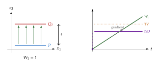
Example 1 (Parallel Lines in 2D).
Let be the uniform distribution on the line segment and let be the uniform distribution on the shifted segment . For every , and have disjoint support, so: Only tells the generator “move the line down by ” and provides a gradient of constant magnitude . The other divergences say “you're completely wrong” with zero gradient.
Historical Note.
The idea of using the Wasserstein distance for training generative models was proposed by Arjovsky et al. [1] in their influential 2017 paper. The name “Earth Mover's Distance” was popularised in computer science by Rubner et al. [2], who used it for image retrieval. The mathematical foundations go back to Gaspard Monge (1781) and Leonid Kantorovich (1942), whose work on optimal transport won him the Nobel Prize in Economics.
Recap: The Wasserstein-1 Distance
We introduced the Wasserstein distance in the divergences chapter (Definition 8). Here we recall the key facts needed for WGAN.
Definition 1 (Wasserstein-1 Distance).
Given two probability distributions and on a metric space , the Wasserstein-1 distance (Earth Mover's distance) is (W1) where is the set of all joint distributions (couplings) with marginals and .
Remark 1 (Intuition: Piles of Sand).
Think of as a pile of sand and as a hole of the same total volume. A coupling specifies how much sand to move from each location to each location , and is the cost of moving one unit of sand. The Wasserstein distance is the cheapest way to fill the hole.
The Wasserstein distance has a property that makes it uniquely suited for generative modelling:
Proposition 1 (Wasserstein Metrises Weak Convergence).
On a compact metric space , a sequence of distributions converges weakly to (i.e. for every bounded continuous ) if and only if .
This means that minimising is equivalent to making the generator distribution converge to the data distribution in the weakest reasonable sense. In contrast, KL and JS divergence can be infinite or discontinuous even along sequences that converge weakly.
Kantorovich–Rubinstein Duality
The primal form requires optimising over the infinite-dimensional space of couplings, computationally intractable in general. The Kantorovich–Rubinstein (KR) duality provides an equivalent formulation that replaces the coupling with a single function, making it amenable to neural-network approximation.
Theorem 1 (Kantorovich–Rubinstein Duality).
For probability distributions and on a compact metric space , (KR) where the supremum is over all -Lipschitz functions (see Definition 20).
Insight.
The dual form says: among all functions that cannot change faster than the metric , find the one that maximally separates the two distributions. This “witness function” is exactly what the WGAN critic learns.
Proof of KR Duality
The proof proceeds in three steps: (1) construct the Lagrangian dual, (2) show the lower bound , (3) show the upper bound using the infimal convolution.
Proof.
Step 1: Lagrangian dual. The primal problem is subject to the marginal constraints Introducing Lagrange multipliers and (see Definition def:lagrange), the Lagrangian is (Lagrangian) Collecting terms: (Collected) The objective is convex, and the constraints are affine, so Slater's condition holds trivially (Definition 17, Theorem 15). By strong duality (Theorem 16): (Strongdual)
For the inner infimum over : if for some , we could concentrate mass there and send . Therefore the supremum is restricted to pairs satisfying for all , and the infimum over yields: (DUAL)
Step 2: Lower bound. Let be any -Lipschitz function. For any coupling with marginals and : (LB1) where uses the marginal constraints, and uses the -Lipschitz property . Since is independent of , the inequality holds for the infimum over : (Lowerbound)
Step 3: Upper bound via infimal convolution. Given any feasible with , define the infimal convolution: (Infconv)
Claim: is -Lipschitz. Indeed, for any : for all , so , i.e. . By symmetry, .
Now we show and for all . From the feasibility constraint: Setting in : . Therefore: (FGK) Since is -Lipschitz, combining with : Both inequalities are equalities, completing the proof.
Remark 2 (Reading the Dual).
The KR dual says: “Find the function whose Lipschitz constant is at most that maximises the difference in expected values under and .” Intuitively, “tilts” the space so that mass under rolls uphill and mass under rolls downhill, and the Lipschitz constraint limits how steep the tilt can be.
The WGAN Objective
The Kantorovich–Rubinstein duality directly suggests a GAN-like training procedure. Replace the supremum over all -Lipschitz functions with a neural network (called the critic), and replace with the generator distribution .
Definition 2 (WGAN Value Function).
The WGAN objective is the saddle-point problem (Value) where is a set of parameters such that are all -Lipschitz for some .
Example 2 (Comparing GAN and WGAN Objectives).
Side by side, the two objectives reveal their structural difference:
1.6
Original GAN WGAN Critic output via sigmoid (no activation) Critic loss Generator loss Divergence Jensen–Shannon Wasserstein-1 Constraint None (discriminator is a classifier) Lipschitz on
Caution.
The WGAN critic has no sigmoid output layer. Its output is an unbounded real number (a “score”), not a probability. Using a sigmoid would destroy the Wasserstein interpretation and revert to something closer to the original GAN.
Insight.
The WGAN loss is an estimate of the Wasserstein distance. Unlike the GAN discriminator loss, which provides no information about sample quality once the discriminator is perfect, the WGAN critic loss correlates directly with generation quality. You can literally watch the loss curve go down and know that images are improving, a luxury that original GANs never offered.
Enforcing the Lipschitz Constraint
The entire WGAN framework hinges on constraining the critic to be Lipschitz. This seemingly simple requirement turns out to be the central practical challenge, and several ingenious solutions have been proposed.
Weight Clipping
The original WGAN paper [1] enforces the Lipschitz constraint by clipping all critic weights to a compact range after each gradient update.
Definition 3 (Weight Clipping).
After each parameter update , set (CLIP) applied element-wise, where is a hyperparameter (typically ).
Remark 3 (Why Clipping Enforces Lipschitz).
A neural network with bounded weights has bounded operator norms for each layer. If each weight matrix satisfies , then the Lipschitz constant of each affine layer is bounded, and the overall Lipschitz constant is bounded by the product of per-layer constants (Exercise 1).
Unfortunately, weight clipping has serious drawbacks:
Caution.
Weight clipping is a blunt instrument:
Capacity underuse. If is too small, the critic can only represent very simple functions, wasting the network's capacity. In practice, clipped critics tend to learn functions that are nearly linear.
Exploding/vanishing gradients. If is too large, the Lipschitz constant becomes very large and the Wasserstein estimate is poor; if is too small, gradients can vanish through many layers.
Sensitivity to . Performance depends critically on the clipping range, and the optimal varies across datasets and architectures.
Gradient Penalty (WGAN-GP)
Gulrajani et al. [3] proposed a much more effective approach: instead of hard-clipping the weights, penalise the critic's gradient norm to encourage the -Lipschitz constraint directly.
The key theoretical motivation comes from the following result about the optimal critic:
Proposition 2 (Gradient Norm of the Optimal Critic).
Let and be distributions on a compact metric space, the optimal -Lipschitz critic, and an optimal coupling. If is differentiable, then for with : (Optgrad) That is, the optimal critic has gradient norm exactly almost everywhere along straight lines between coupled points.
Proof.
Since is compact, an optimal -Lipschitz critic and optimal coupling exist. For , optimality gives: Define for . Since is -Lipschitz: so is -Lipschitz with and . Writing: both inequalities must be equalities, so , i.e. .
Let . The directional derivative: Since is -Lipschitz, . By the Pythagorean decomposition (Exercise 6): The squeeze gives , so .
This proposition tells us that the optimal critic has gradient norm exactly along the optimal transport paths. This motivates penalising deviations from unit gradient norm:
Definition 4 (WGAN-GP Objective).
The WGAN-GP critic loss is (GP) where with , and is the penalty coefficient (typically ).
Example 3 (Understanding the Gradient Penalty).
The gradient penalty is evaluated at interpolated points between real and fake samples. Why interpolations?
Proposition 2 shows the optimal critic has unit gradient norm along straight lines between optimally coupled points .
We approximate the optimal coupling by pairing each real sample with a generated sample and interpolating between them.
The penalty is a two-sided penalty: it pushes the gradient norm towards , not just below . This is important because the optimal critic satisfies , not merely .
Remark 4 (One-Sided vs. Two-Sided Penalty).
One might consider the one-sided penalty , which only penalises violations of the Lipschitz constraint. However, the two-sided penalty works better in practice: it constrains the critic to the optimal function class (gradient norm exactly ) rather than the broader class of all -Lipschitz functions, reducing the effective search space.
Spectral Normalisation
Miyato et al. [4] proposed a third approach that is both computationally efficient and effective: normalise each weight matrix by its spectral norm (largest singular value).
Definition 5 (Spectral Normalisation).
For a weight matrix , define the spectrally normalised weight: (SN) where is the largest singular value of .
Proposition 3 (Lipschitz Constant Under Spectral Normalisation).
A feed-forward network where each layer uses a -Lipschitz activation (e.g. ReLU, leaky ReLU) has Lipschitz constant at most : (LIP)
Proof.
Each spectrally normalised layer satisfies by construction, so is -Lipschitz (since is -Lipschitz and ). The composition of -Lipschitz functions is -Lipschitz.
In practice, computing exactly at every iteration is expensive. Instead, one uses the power iteration method:
Algorithm 1 (Spectral Norm Estimation via Power Iteration).
Initialise randomly with .
At each training step, perform one update:
Estimate .
Set .
One power-iteration step per training step suffices because changes slowly, so the estimate tracks accurately.
Remark 5 (Comparing Lipschitz Enforcement Methods).
1.3
Weight Clipping Gradient Penalty Spectral Norm Proposed by [1] [3] [4] Constraint type Hard (project) Soft (penalty) Hard (normalise) Per-step cost Negligible Expensive (Jacobian) Cheap (1 power iter.) Critic capacity Low (underfits) Full Full Batch normalisation Compatible Incompatible Compatible Hyperparameters (sensitive) (robust at 10) None
WGAN Algorithms
We now present the two main WGAN training algorithms.
WGAN with Weight Clipping
Algorithm 2 (WGAN Training (Weight Clipping)).
Hyperparameters: learning rate , clipping parameter , batch size , critic iterations .
- Initialise critic parameters , generator parameters
- while has not converged
- for
- Sample
- Sample
- Sample
Remark 6 (Why ?).
Unlike the original GAN where the discriminator trains for step per generator step, WGAN requires more critic updates. The Wasserstein estimate is only meaningful when the critic is close to optimal. In practice, provides a good trade-off between estimation quality and training speed.
WGAN-GP Algorithm
Algorithm 3 (WGAN-GP Training (Gradient Penalty)).
Hyperparameters: learning rate , gradient penalty coefficient , batch size , critic iterations . Use Adam with , .
- Initialise critic parameters , generator parameters
- while has not converged
- for
- Sample , ,
- Interpolate
- Sample
Caution.
WGAN-GP is incompatible with batch normalisation in the critic. Batch normalisation introduces dependencies between samples in a mini-batch, which means the critic's gradient at depends on other samples in the batch. This violates the assumption that the gradient penalty is evaluated independently for each interpolated point. Use layer normalisation or instance normalisation instead.
Training Dynamics and the Meaningful Loss
One of the most celebrated practical advantages of WGAN is its meaningful loss curve.
Key Idea.
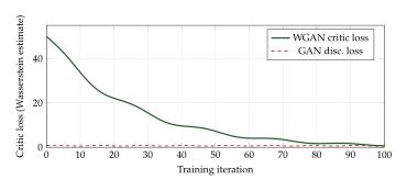
In a standard GAN, the discriminator loss converges to regardless of sample quality, so the loss provides no information about training progress. In WGAN, the critic loss is an estimate of , which decreases monotonically as the generator improves. For the first time, you can monitor a single scalar to assess generation quality.
Example 4 (Monitoring the WGAN Loss).
During WGAN training on a face generation task:
Epoch 1: Critic loss . Generated images are random noise.
Epoch 50: Critic loss . Generated images show blurry face-like shapes.
Epoch 200: Critic loss . Generated images are sharp, recognisable faces.
Epoch 500: Critic loss . Generated images are nearly photorealistic.
The correlation between the critic loss and visual quality is remarkably strong, a property that original GANs lack entirely.
The convergence properties of WGAN are also theoretically grounded:
Theorem 2 (Convergence of WGAN).
Let be a distribution parameterised by such that is continuous in . If the critic is trained to optimality at each step, then the generator gradient exists and is continuous, providing a stable signal for gradient descent.
This is in stark contrast to the original GAN, where the generator gradient can be zero (saturated discriminator) or infinite (near decision boundaries).
Practical Advantages and Limitations
Remark 7 (Advantages of WGAN).
Meaningful loss. The critic loss tracks the Wasserstein distance and correlates with sample quality.
Stability. Training is more stable across architectures and hyperparameters.
Mode coverage. The Wasserstein distance penalises all uncovered modes, reducing (though not eliminating) mode collapse.
No careful balancing needed. In standard GANs, the discriminator and generator must be balanced; in WGAN, the critic should simply be trained to near-optimality.
Remark 8 (Limitations of WGAN).
Slower per iteration. Training the critic for steps per generator step means more critic evaluations.
Gradient penalty cost. WGAN-GP requires computing gradients of gradients (double backpropagation), which is expensive in memory and compute.
Not always superior. On well-tuned benchmarks, standard GANs with spectral normalisation and hinge loss can match or exceed WGAN-GP.
Critic architecture matters. The quality of the Wasserstein estimate depends heavily on the critic's expressiveness.
Example 5 (WGAN on MNIST).
Consider training a WGAN-GP on MNIST (2828 grayscale digits):
Generator: Fully connected, , ReLU activations, tanh output.
Critic: Fully connected, , LeakyReLU, no batch normalisation, no sigmoid.
Training: Adam with , , , , .
After 50,000 iterations, the generator produces sharp, diverse digits, and the critic loss curve is a smooth, monotonically decreasing function, confirming that the Wasserstein framework delivers on its promise of a meaningful training signal.
From WGAN to Modern Practice
The WGAN papers fundamentally changed how the community thinks about GAN training. Their key insight, that the choice of divergence matters enormously and that divergences from optimal transport are uniquely suited to generative modelling, has had lasting influence well beyond GANs.
Remark 9 (The Legacy of WGAN).
Spectral normalisation is now standard in almost all GAN architectures, even those not explicitly trained with the Wasserstein loss.
Optimal transport has become a central tool in machine learning, from domain adaptation to single-cell biology.
The critic loss as a quality metric inspired the FID score (Definition 7), which is itself a Wasserstein-2 distance in feature space (Remark 7).
Diffusion models implicitly use optimal-transport ideas through their score-matching objectives and probability flow ODEs.
Historical Note.
The WGAN paper [1] by Arjovsky, Chintala, and Bottou appeared in January 2017 and quickly became one of the most cited GAN papers. The follow-up WGAN-GP paper [3] by Gulrajani et al. appeared just three months later, in March 2017. Spectral normalisation by Miyato et al. [4] followed in 2018. Together, these three papers form the “Lipschitz trilogy” that solved WGAN's central practical challenge.
Exercises
Exercise 1 (Lipschitz Continuity of Compositions).
Let be -Lipschitz and be -Lipschitz. Show that is -Lipschitz. Conclude that a neural network with layers, each with Lipschitz constant , has overall Lipschitz constant at most .
Exercise 2 (Weight Clipping Does Not Enforce 1-Lipschitz).
Consider a single-layer linear critic with .
- (a)
Show that the Lipschitz constant of is .
- (b)
Show that weight clipping enforces , not .
- (c)
Explain how this gap affects the Wasserstein estimate.
Exercise 3 (Gradient Penalty Derivation).
Starting from Proposition 2, explain why:
- (a)
The gradient penalty is evaluated at interpolated points rather than at real or fake points alone.
- (b)
The two-sided penalty is preferred over the one-sided penalty .
- (c)
The penalty coefficient should be large enough to enforce the constraint but not so large that it dominates the Wasserstein objective.
Exercise 4 (WGAN vs. Original GAN on Point Masses).
Let and on .
- (a)
Compute .
- (b)
Compute .
- (c)
Compute the gradients and for .
- (d)
Explain why this illustrates the advantage of WGAN for training generative models.
Exercise 5 (Wasserstein Distance in One Dimension).
For distributions on with CDFs :
- (a)
Show that . Hint: the optimal transport maps quantiles to quantiles.
- (b)
Compute and show it equals .
- (c)
Compute .
Exercise 6 (Pythagorean Decomposition).
Let be a unit vector in and an arbitrary vector.
- (a)
Show that and are orthogonal.
- (b)
Prove .
- (c)
Use this decomposition to verify the squeeze argument in the proof of Proposition 2.
Exercise 7 (Infimal Convolution Properties).
Exercise 8 (Spectral Norm Computation).
For the matrix :
- (a)
Compute the singular values of .
- (b)
Compute .
- (c)
Verify that .
- (d)
Perform two steps of power iteration starting from and compare with the exact answer.
Exercise 9 (ReLU Networks and Lipschitz Constants).
- (a)
Show that ReLU is -Lipschitz.
- (b)
Show that LeakyReLU with slope is -Lipschitz.
- (c)
For a two-layer network , show that .
- (d)
Is this bound tight? Give an example.
Exercise 10 (Comparing WGAN, WGAN-GP, and SN-GAN).
Consider training a convolutional GAN on CIFAR-10.
- (a)
Describe the critic architecture for each of WGAN (weight clipping), WGAN-GP, and SN-GAN. Which normalisation layers can each use?
- (b)
If the critic has 5 convolutional layers each with kernels, estimate the computational overhead of the gradient penalty versus spectral normalisation.
- (c)
Why does WGAN-GP require Adam with while standard GAN training uses ?
Exercise 11 (The Critic as a Density Ratio Estimator).
In the original GAN, the optimal discriminator computes the density ratio (Proposition 1). What does the optimal WGAN critic compute? Show that it is related to the Kantorovich potential and not a density ratio.
Exercise 12 (Wasserstein-2 and FID).
The Fréchet Inception Distance (FID, Definition 7) is
- (a)
Show that this equals .
- (b)
Explain why using in Inception feature space rather than pixel space is advantageous.
Exercise 13 (WGAN for Discrete Data).
Suppose and are distributions over a finite set with metric .
- (a)
Write as a linear program.
- (b)
Show that the KR dual specialises to .
- (c)
For and , compute and find the optimal .
Exercise 14 (Implementing WGAN-GP in PyTorch).
Write PyTorch pseudocode for:
- (a)
The gradient penalty computation, using
torch.autograd.gradto compute . - (b)
A training loop that alternates between critic and generator updates.
- (c)
Explain why
create_graph=Truemust be passed totorch.autograd.gradfor the gradient penalty.
References
-
Wasserstein GAN
BibTeX
@article{arjovsky2017wasserstein, title = {Wasserstein GAN}, author = {Arjovsky, Martin and Chintala, Soumith and Bottou, L\'eon}, journal = {arXiv:1701.07875}, year = {2017} }Journal article
-
The Earth Mover's Distance as a Metric for Image Retrieval
BibTeX
@article{rubner2000earth, title = {The Earth Mover's Distance as a Metric for Image Retrieval}, author = {Rubner, Yossi and Tomasi, Carlo and Guibas, Leonidas J.}, journal = {International Journal of Computer Vision}, volume = {40}, number = {2}, pages = {99--121}, year = {2000}, publisher = {Springer} }Journal article
-
Improved training of Wasserstein GANs
BibTeX
@inproceedings{gulrajani2017improved, title={Improved training of Wasserstein GANs}, author={Gulrajani, Ishaan and Ahmed, Faruk and Arjovsky, Martin and Dumoulin, Vincent and Courville, Aaron C}, booktitle={Advances in neural information processing systems}, pages={5767--5777}, year={2017} }Conference paper
-
Spectral normalization for generative adversarial networks
BibTeX
@inproceedings{miyato2018spectral, title={Spectral normalization for generative adversarial networks}, author={Miyato, Takeru and Kataoka, Toshiki and Koyama, Masanori and Yoshida, Yuichi}, booktitle={Proceedings of the International Conference on Learning Representations}, year={2018}, url={https://openreview.net/forum?id=B1QRgziT-} }Conference paper