A Mathematical Analysis

This appendix collects the core results from real analysis and topology that underpin the mathematics of generative modelling. Rather than simply listing definitions, we develop the material from the ground up, with complete proofs and worked examples, so that the reader can appreciate why each concept matters. The journey begins with the real number line and ends, several sections later, with the function-space machinery needed for variational inference and optimal transport.

The Real Number Line

The real numbers $ℝ$ are so familiar that one might wonder why we bother axiomatising them at all. The answer is that one particular property of $ℝ$ , completeness, is responsible for virtually every convergence guarantee we rely on when training generative models. Without it, gradient descent could converge to a “hole” in the number line, and probability distributions could fail to have well-defined means.

We begin with two companion definitions that capture the idea of “tightest possible bound.”

Definition 1 (Supremum).

Let $S \subseteq ℝ$ be a nonempty set. A number $s \in ℝ$ is the supremum (or least upper bound) of $S$ , written $s = \sup S$ , if

$x \leq s$ for every $x \in S$ (i.e. $s$ is an upper bound), and
whenever $t$ is an upper bound of $S$ we have $s \leq t$ (i.e. $s$ is the smallest such bound).

The supremum need not belong to $S$ itself.

Definition 2 (Infimum).

Let $S \subseteq ℝ$ be nonempty. The infimum (or greatest lower bound) of $S$ , written $\inf S$ , is the largest real number $ℓ$ satisfying $ℓ \leq x$ for every $x \in S$ . Equivalently, $\inf S = - \sup (- S)$ where $- S = {- x : x \in S}$ .

Example 1 (Open Interval).

Consider the open interval $S = (0, 1)$ . Every element of $S$ is strictly less than $1$ , and for any proposed upper bound $t < 1$ the midpoint $\frac{t + 1}{2}$ lies in $S$ yet exceeds $t$ . Hence $\sup S = 1$ , even though $1 \notin S$ . By a symmetric argument, $\inf S = 0 \notin S$ .

Example 2 (Rationals in an Interval).

Let $U = {x \in ℚ : 0 < x < \sqrt{2}}$ . Every element of $U$ is rational, yet $\sup U = \sqrt{2}$ , which is irrational. This example is historically significant: it shows that the rationals alone cannot supply the supremum of a bounded set of rationals.

Example 3 (Negative Powers of Two).

Let $V = {2^{- n} : n \in ℕ} = {1, \frac{1}{2}, \frac{1}{4}, \dots}$ . Then $\sup V = 1 \in V$ and $\inf V = 0 \notin V$ , since the terms decrease toward zero but never reach it.

The following axiom is what distinguishes $ℝ$ from $ℚ$ .

Theorem 1 (Completeness Axiom).

Every nonempty subset of $ℝ$ that is bounded above has a supremum in $ℝ$ .

The Completeness Axiom is not something we prove; it is taken as an axiom in the construction of $ℝ$ . One way to appreciate its content is to observe that the analogous statement fails for $ℚ$ : the set ${q \in ℚ : q^{2} < 2}$ is bounded above in $ℚ$ yet has no rational least upper bound.

Key Idea.

Completeness is what distinguishes $ℝ$ from $ℚ$ : it guarantees that limits of convergent sequences always exist within $ℝ$ , which is essential for the convergence guarantees we need in optimisation and sampling.

An immediate and useful consequence is the Archimedean property, which says that there are no “infinitely large” or “infinitesimally small” positive reals.

Theorem 2 (Archimedean Property).

For every $x \in ℝ$ with $x > 0$ and every $y \in ℝ$ , there exists $n \in ℕ$ such that $n x > y$ .

Proof.

Suppose for contradiction that no such $n$ exists. Then $n x \leq y$ for every $n \in ℕ$ , which means the set $S = {n x : n \in ℕ}$ is bounded above by $y$ . By the Completeness Axiom (Theorem 1), $s = \sup S$ exists in $ℝ$ . Because $x > 0$ , we have $s - x < s$ , so $s - x$ is not an upper bound of $S$ . Therefore there exists $m \in ℕ$ with $m x > s - x$ , giving $(m + 1) x > s$ . But $(m + 1) x \in S$ , contradicting the assumption that $s$ is an upper bound.

∎

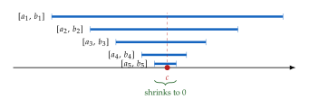
The next result uses completeness in a geometric way. It says that a sequence of closed intervals, each contained in the previous one and shrinking in length, must “trap” a single point.

Theorem 3 (Nested Intervals).

Let $[a_{1}, b_{1}] \supseteq [a_{2}, b_{2}] \supseteq [a_{3}, b_{3}] \supseteq \dots$ be a nested sequence of nonempty closed intervals with $\lim_{n \to \infty} (b_{n} - a_{n}) = 0$ . Then there exists a unique point $c \in ℝ$ with $⋂_{n = 1}^{\infty} [a_{n}, b_{n}] = {c} .$

Proof.

The sequence $(a_{n})$ is non-decreasing and bounded above by $b_{1}$ , so by the Completeness Axiom it converges to $c = \sup {a_{n}}$ . Similarly, $(b_{n})$ is non-increasing and bounded below by $a_{1}$ , so it converges to some limit $c^{'} = \inf {b_{n}}$ . For every $n$ we have $a_{n} \leq c \leq c^{'} \leq b_{n}$ , hence $0 \leq c^{'} - c \leq b_{n} - a_{n} \to 0$ , giving $c = c^{'}$ . Any point in the intersection must lie in every $[a_{n}, b_{n}]$ and hence equal $c$ .

∎

The Nested Intervals Theorem: a sequence of closed intervals

[a_{n}, b_{n}]

, each contained in the previous one and shrinking in length, traps a unique limit point

c

. The dashed line marks the common intersection.

Historical Note.

Richard Dedekind (1872) and Georg Cantor independently constructed $ℝ$ from $ℚ$ , each motivated by the need for a number system where every Cauchy sequence converges. Dedekind used “cuts” that partition $ℚ$ into two halves, while Cantor identified each real with an equivalence class of Cauchy sequences of rationals. Both constructions yield the same ordered field, and the Completeness Axiom holds in each.

Metric Spaces

A great deal of generative modelling takes place not on the real line but in high-dimensional spaces: image pixel spaces, latent spaces, and spaces of probability distributions. To discuss convergence, continuity, and compactness in all these settings at once, we need the abstraction of a metric space. The idea is simple: distill the essence of “distance” into a small set of axioms, and then develop the theory once and for all.

Definition and Examples

Definition 3 (Metric Space).

A metric space is a pair $(X, d)$ where $X$ is a nonempty set and $d : X \times X \to ℝ$ is a function (called a metric or distance function) satisfying, for all $x, y, z \in X$ :

Non-negativity: $d (x, y) \geq 0$ .
Identity of indiscernibles: $d (x, y) = 0$ if and only if $x = y$ .
Symmetry: $d (x, y) = d (y, x)$ .
Triangle inequality: $d (x, z) \leq d (x, y) + d (y, z)$ .

These four axioms capture the intuitive properties we expect of distance: distances are non-negative, zero only for identical points, symmetric, and satisfy the “shortcut cannot be longer than the detour” principle. Let us see several concrete instances.

Example 4 (Euclidean Metric).

On $ℝ^{n}$ , the Euclidean metric is $d (𝒙, 𝒚) = \sqrt{\sum_{i = 1}^{n} {(x_{i} - y_{i})}^{2}} = {‖ 𝒙 - 𝒚 ‖}_{2} .$ This is the distance “as the crow flies” and the default metric in most machine learning applications.

Example 5 (Discrete Metric).

On any set $X$ , define $d (x, y) = {\begin{matrix} 0 & if x = y, \\ 1 & if x \neq y . \end{matrix}$ Verification of the axioms is immediate. The discrete metric may seem artificial, but it appears naturally when $X$ is a finite label set (e.g. class labels in a classifier).

Example 6 (Taxicab Metric).

On $ℝ^{n}$ , the taxicab (or Manhattan) metric is $d_{1} (𝒙, 𝒚) = \sum_{i = 1}^{n} | x_{i} - y_{i} | = {‖ 𝒙 - 𝒚 ‖}_{1} .$ In two dimensions, this measures distance by travelling along axis-aligned streets, like a taxi in Manhattan.

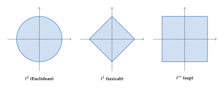
Example 7 ( $ℓ^{p}$ Metric).

For any $p \geq 1$ , the $ℓ^{p}$ distance on $ℝ^{n}$ is $d_{p} (𝒙, 𝒚) = (\sum_{i = 1}^{n} {| x_{i} - y_{i} |}^{p})^{1 / p} = {‖ 𝒙 - 𝒚 ‖}_{p} .$ The Euclidean metric corresponds to $p = 2$ and the taxicab metric to $p = 1$ . The limiting case $p \to \infty$ gives the supremum metric $d_{\infty} (𝒙, 𝒚) = \max_{i} | x_{i} - y_{i} |$ . That the triangle inequality holds for all $p \geq 1$ is the content of the Minkowski inequality.

The shape of the unit ball ${x \in ℝ^{2} : d (0, x) \leq 1}$ varies dramatically with the choice of metric.

Unit balls

{𝒙 \in ℝ^{2} : {‖ 𝒙 ‖}_{p} \leq 1}

for three choices of

p

. The Euclidean ball is a circle, the

ℓ^{1}

ball is a diamond (rotated square), and the

ℓ^{\infty}

ball is an axis-aligned square.

Open and Closed Sets

With a metric in hand, we can formalise what it means for a set to “have no boundary points” (open) or “contain all its boundary points” (closed). These notions are essential for stating convergence theorems precisely.

Definition 4 (Open Ball).

Let $(X, d)$ be a metric space, $x \in X$ , and $ε > 0$ . The open ball of radius $ε$ centred at $x$ is $B (x, ε) = {y \in X : d (x, y) < ε} .$

Definition 5 (Open Set).

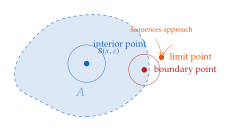
A subset $U \subseteq X$ is open if for every $x \in U$ there exists $ε > 0$ such that $B (x, ε) \subseteq U$ . Informally, every point of $U$ can be “wiggled” a little without leaving $U$ .

Definition 6 (Closed Set).

A subset $C \subseteq X$ is closed if its complement $X ∖ C$ is open.

A common misconception is that “closed” is the opposite of “open.” In fact, a set can be both open and closed (the empty set and $X$ itself), or neither (the half-open interval $[0,1)$ in $ℝ$ ).

Definition 7 (Limit Point).

A point $x \in X$ is a limit point (or accumulation point) of a set $A \subseteq X$ if every open ball centred at $x$ contains a point of $A$ other than $x$ itself: $B (x, ε) \cap (A ∖ {x}) \neq \emptyset for all ε > 0.$ Note that $x$ need not belong to $A$ .

Definition 8 (Isolated Point).

A point $x \in A$ is an isolated point of $A$ if there exists $ε > 0$ with $B (x, ε) \cap A = {x}$ . Equivalently, $x \in A$ but $x$ is not a limit point of $A$ .

Anatomy of a set in a metric space. An interior point (blue) has an

ε

-ball entirely inside

A

. A boundary point (red) lies on the edge: every ball around it intersects both

A

and

X ∖ A

. A limit point (orange) outside

A

can be approached by sequences from within

A

Interior, Closure, and Boundary

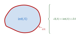
Every set $A$ in a metric space has three closely related derived sets that describe its “inner core,” its “completed version,” and the “edge” between inside and outside.

Definition 9 (Interior).

The interior of $A$ , denoted $int (A)$ , is the set of all points $x \in A$ for which there exists $ε > 0$ with $B (x, ε) \subseteq A$ . Equivalently, $int (A)$ is the largest open set contained in $A$ (i.e. the union of all open subsets of $A$ ).

Definition 10 (Closure).

The closure of $A$ , denoted $A$ or $cl (A)$ , is the smallest closed set containing $A$ . Equivalently, $cl (A) = A \cup A^{'}$ , where $A^{'}$ is the set of all limit points of $A$ .

Definition 11 (Boundary).

The boundary of $A$ is $\partial A = cl (A) ∖ int (A)$ . A point $x$ belongs to $\partial A$ if and only if every open ball centred at $x$ intersects both $A$ and $X ∖ A$ .

The interior

int (A)

(blue region), boundary

\partial A

(thick red curve), and closure

cl (A) = int (A) \cup \partial A

With these definitions in place, we can prove two fundamental characterisations of closed sets.

Theorem 4 (Closed Set Characterisation).

A set $A$ in a metric space $(X, d)$ is closed if and only if $A$ contains all its limit points.

Proof.

( $\Rightarrow$ ) Suppose $A$ is closed and let $x$ be a limit point of $A$ . We must show $x \in A$ . If $x \notin A$ , then $x \in X ∖ A$ , which is open. So there exists $ε > 0$ with $B (x, ε) \subseteq X ∖ A$ , meaning $B (x, ε) \cap A = \emptyset$ . But this contradicts $x$ being a limit point, since every ball around a limit point must intersect $A$ .

( $\Leftarrow$ ) Suppose $A$ contains all its limit points. We show $X ∖ A$ is open. Take any $y \in X ∖ A$ . Since $y \notin A$ and $y$ is not a limit point of $A$ (because $A$ contains all its limit points), there exists $ε > 0$ with $B (y, ε) \cap (A ∖ {y}) = \emptyset$ . Since $y \notin A$ , this gives $B (y, ε) \cap A = \emptyset$ , i.e. $B (y, ε) \subseteq X ∖ A$ . As $y$ was arbitrary, $X ∖ A$ is open, so $A$ is closed.

∎

Theorem 5 (Closure via Limit Points).

For any subset $A$ of a metric space $(X, d)$ , $cl (A) = A \cup A^{'},$ where $A^{'}$ denotes the set of all limit points of $A$ .

Proof.

We show both inclusions.

( $\supseteq$ ) We must show $A \cup A^{'} \subseteq cl (A)$ . Since $cl (A)$ is closed and contains $A$ , it suffices to show it contains every limit point of $A$ . Let $x \in A^{'}$ and suppose $x \notin cl (A)$ . Then $x \in X ∖ cl (A)$ , which is open. So there exists $ε > 0$ with $B (x, ε) \subseteq X ∖ cl (A) \subseteq X ∖ A$ , contradicting the fact that $x$ is a limit point of $A$ .

( $\subseteq$ ) We show $cl (A) \subseteq A \cup A^{'}$ by proving that $A \cup A^{'}$ is closed. Let $x$ be a limit point of $A \cup A^{'}$ . For every $ε > 0$ , $B (x, ε)$ contains a point $y \in A \cup A^{'}$ with $y \neq x$ . If $y \in A$ , then $B (x, ε) \cap A \neq \emptyset$ . If $y \in A^{'}$ , then pick $δ > 0$ small enough that $B (y, δ) \subseteq B (x, ε)$ ; since $y$ is a limit point of $A$ , $B (y, δ)$ contains a point of $A$ distinct from $y$ , and hence $B (x, ε) \cap A \neq \emptyset$ . Either way, $x$ is a limit point of $A$ , so $x \in A^{'}$ . Therefore $A \cup A^{'}$ contains all its limit points and is closed by Theorem 4. Since $cl (A)$ is the smallest closed set containing $A$ , we conclude $cl (A) \subseteq A \cup A^{'}$ .

∎

Sequences and Convergence

Sequences are the primary vehicle through which we discuss convergence in analysis. A training loop in deep learning is, at bottom, a sequence of parameter vectors $𝜽_{1}, 𝜽_{2}, 𝜽_{3}, \dots$ , and the central question is whether this sequence converges to a useful model. The concepts in this section make that question precise.

Definition 12 (Convergent Sequence).

A sequence ${(x_{n})}_{n = 1}^{\infty}$ in a metric space $(X, d)$ converges to a point $x \in X$ if for every $ε > 0$ there exists $N \in ℕ$ such that $d (x_{n}, x) < ε$ for all $n \geq N$ . We write $x_{n} \to x$ or $\lim_{n \to \infty} x_{n} = x$ .

Convergence is the demand that, no matter how tight a tolerance $ε$ we specify, the sequence eventually enters and stays within the open ball $B (x, ε)$ .

Example 8 (Convergent and Divergent Sequences).

The sequence $x_{n} = 1 / n$ in $ℝ$ converges to $0$ : given $ε > 0$ , choose $N > 1 / ε$ (possible by the Archimedean property, Theorem 2), and then $| x_{n} - 0 | = 1 / n < ε$ for all $n \geq N$ .

The sequence $y_{n} = {(- 1)}^{n}$ does not converge. Its terms alternate between $+ 1$ and $- 1$ and never settle within any ball of radius less than $1$ around a single point.

A convergent sequence: for

n \geq N

(marked in red), every term

x_{n}

lies within the

ε

-band (blue shading) around the limit

x^{*}

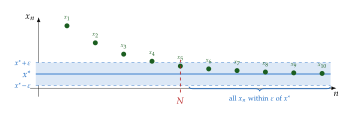
A subtler notion asks whether the terms of a sequence get close to each other, without reference to any particular limit.

Definition 13 (Cauchy Sequence).

A sequence $(x_{n})$ in a metric space $(X, d)$ is a Cauchy sequence if for every $ε > 0$ there exists $N \in ℕ$ such that $d (x_{n}, x_{m}) < ε$ for all $n, m \geq N$ .

Every convergent sequence is Cauchy, but the converse can fail: the space may have “gaps” that prevent a Cauchy sequence from finding its limit.

Theorem 6 (Convergent Implies Cauchy).

Every convergent sequence in a metric space is a Cauchy sequence.

Proof.

Suppose $x_{n} \to x$ . Given $ε > 0$ , choose $N$ such that $d (x_{n}, x) < ε / 2$ for all $n \geq N$ . Then for $n, m \geq N$ , $d (x_{n}, x_{m}) \leq d (x_{n}, x) + d (x, x_{m}) < \frac{ε}{2} + \frac{ε}{2} = ε,$ where we used the triangle inequality.

∎

Remark 1 (The Converse Fails in $ℚ$ ).

The sequence $1, 1.4, 1.41, 1.414, 1.4142, \dots$ of decimal approximations to $\sqrt{2}$ is a Cauchy sequence of rationals. Yet it does not converge in $ℚ$ , because its limit $\sqrt{2}$ is irrational. This is precisely the kind of gap that the completeness of $ℝ$ eliminates.

Definition 14 (Complete Metric Space).

A metric space $(X, d)$ is complete if every Cauchy sequence in $X$ converges to a limit in $X$ .

Completeness is a property of the space, not of individual sequences. The rationals are incomplete; the reals are complete. In the infinite-dimensional world, Banach and Hilbert spaces are complete by definition, and this is exactly what makes them suitable homes for the function spaces used in variational inference.

Theorem 7 (Completeness of $ℝ^{n}$ ).

$ℝ^{n}$ with the Euclidean metric is a complete metric space.

Proof sketch.

Let ${(𝒙^{(k)})}_{k = 1}^{\infty}$ be a Cauchy sequence in $ℝ^{n}$ . For each coordinate $i \in {1, \dots, n}$ , the scalar sequence ${(x_{i}^{(k)})}_{k = 1}^{\infty}$ is Cauchy in $ℝ$ (since $| x_{i}^{(k)} - x_{i}^{(m)} | \leq {‖ 𝒙^{(k)} - 𝒙^{(m)} ‖}_{2}$ ). By the completeness of $ℝ$ (which follows from the Completeness Axiom, Theorem 1), each coordinate sequence converges: $x_{i}^{(k)} \to x_{i}^{*} \in ℝ$ . Setting $𝒙^{*} = (x_{1}^{*}, \dots, x_{n}^{*})$ , one verifies ${‖ 𝒙^{(k)} - 𝒙^{*} ‖}_{2} \to 0$ .

∎

The next result is one of the jewels of real analysis. It guarantees the existence of convergent subsequences in bounded regions.

Theorem 8 (Bolzano–Weierstrass).

Every bounded sequence in $ℝ^{n}$ has a convergent subsequence.

Proof.

We prove the result for $n = 1$ ; the general case follows by applying the one-dimensional argument to each coordinate in turn (using a diagonal subsequence extraction).

Let $(x_{k})$ be a bounded sequence in $ℝ$ , so $x_{k} \in [a, b]$ for all $k$ . We construct a convergent subsequence by interval bisection. Divide $[a, b]$ into two equal halves: $[a, \frac{a + b}{2}]$ and $[\frac{a + b}{2}, b]$ . At least one half contains infinitely many terms of the sequence; call it $[a_{1}, b_{1}]$ and choose $x_{k_{1}} \in [a_{1}, b_{1}]$ . Repeat: bisect $[a_{1}, b_{1}]$ , pick the half with infinitely many terms, call it $[a_{2}, b_{2}]$ , and choose $x_{k_{2}}$ with $k_{2} > k_{1}$ .

Continuing, we obtain a subsequence $(x_{k_{j}})$ and nested intervals $[a_{j}, b_{j}]$ with $b_{j} - a_{j} = (b - a) / 2^{j} \to 0$ and $x_{k_{j}} \in [a_{j}, b_{j}]$ for every $j$ . By the Nested Intervals Theorem (Theorem 3), the intervals shrink to a single point $c$ . Since $| x_{k_{j}} - c | \leq b_{j} - a_{j} \to 0$ , we have $x_{k_{j}} \to c$ .

For $ℝ^{n}$ : given a bounded sequence $(𝒙^{(k)})$ in $ℝ^{n}$ , first extract a subsequence along which the first coordinate converges (by the one-dimensional result). From that subsequence, extract a further subsequence along which the second coordinate also converges. After $n$ such extractions, we have a subsequence that converges in every coordinate, and hence in $ℝ^{n}$ .

∎

Historical Note.

Bernhard Bolzano proved the one-dimensional result in 1817, making it one of the earliest rigorous statements about the structure of $ℝ$ . Karl Weierstrass rediscovered and popularised it in the 1860s as part of his programme to place analysis on a firm logical foundation. The theorem was among the first results to show that $ℝ$ has fundamentally different properties from $ℚ$ : a bounded sequence of rationals need not have a rational limit point.

Compactness

Compactness is arguably the single most important topological property in analysis. Compact sets are “the next best thing to finite sets”: they are small enough to be controlled, yet rich enough to be useful. In optimisation, compactness guarantees that continuous functions attain their optima. In measure theory, compactness ensures that sequences of probability measures have convergent subsequences.

We begin with the covering definition, which is the most general.

Definition 15 (Open Cover).

Let $(X, d)$ be a metric space and $K \subseteq X$ . A collection ${U_{α}}_{α \in I}$ of open sets is an open cover of $K$ if $K \subseteq ⋃_{α \in I} U_{α}$ . A subcover is a subcollection that still covers $K$ .

Definition 16 (Compact Set).

A subset $K$ of a metric space $(X, d)$ is compact if every open cover of $K$ has a finite subcover: whenever $K \subseteq ⋃_{α \in I} U_{α}$ with each $U_{α}$ open, there exist finitely many indices $α_{1}, \dots, α_{m}$ with $K \subseteq U_{α_{1}} \cup \dots \cup U_{α_{m}}$ .

The power of this definition lies in the word “every”: no matter how wastefully we cover $K$ with open sets, we can always trim the cover down to a finite one.

Left: a closed interval

[a, b]

covered by many overlapping open sets. Right: a finite subcover (green, highlighted) suffices. Compactness guarantees that such a finite selection is always possible.

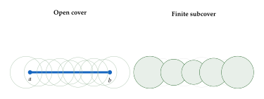
The most useful characterisation of compact subsets of $ℝ^{n}$ is the classical Heine–Borel theorem.

Theorem 9 (Heine–Borel).

A subset $K \subseteq ℝ^{n}$ is compact if and only if it is closed and bounded.

Proof.

( $\Rightarrow$ : compact implies closed and bounded.)

Bounded. Consider the open cover ${B (𝟎, m)}_{m = 1}^{\infty}$ of $K$ . By compactness, finitely many balls suffice: $K \subseteq B (𝟎, m_{1}) \cup \dots \cup B (𝟎, m_{k}) = B (𝟎, M)$ where $M = \max {m_{1}, \dots, m_{k}}$ . Hence $K$ is bounded.

Closed. We show $ℝ^{n} ∖ K$ is open. Fix any $𝒚 \notin K$ . For each $𝒙 \in K$ , let $r_{𝒙} = d (𝒙, 𝒚) / 2 > 0$ and consider the open balls $U_{𝒙} = B (𝒙, r_{𝒙})$ . These cover $K$ , so by compactness there exist $𝒙_{1}, \dots, 𝒙_{m}$ with $K \subseteq U_{𝒙_{1}} \cup \dots \cup U_{𝒙_{m}}$ . Let $ε = \min {r_{𝒙_{1}}, \dots, r_{𝒙_{m}}} > 0$ . We claim $B (𝒚, ε) \subseteq ℝ^{n} ∖ K$ . Indeed, if $𝒛 \in B (𝒚, ε) \cap K$ , then $𝒛 \in U_{𝒙_{j}}$ for some $j$ , giving $d (𝒙_{j}, 𝒚) \leq d (𝒙_{j}, 𝒛) + d (𝒛, 𝒚) < r_{𝒙_{j}} + ε \leq 2 r_{𝒙_{j}} = d (𝒙_{j}, 𝒚)$ , a contradiction.

( $\Leftarrow$ : closed and bounded implies compact.)

Since $K$ is bounded, it is contained in some closed box ${[- M, M]}^{n}$ . Suppose for contradiction that $K$ has an open cover ${U_{α}}$ with no finite subcover. Bisect the box into $2^{n}$ congruent sub-boxes. At least one sub-box intersects $K$ in a subset that has no finite subcover from ${U_{α}}$ ; call this sub-box $B_{1}$ and the corresponding subset $K_{1} = K \cap B_{1}$ . Repeat to obtain nested boxes $B_{1} \supseteq B_{2} \supseteq \dots$ with diameters shrinking to zero and $K_{j} = K \cap B_{j}$ having no finite subcover.

By the Nested Intervals Theorem applied coordinate-wise, the boxes shrink to a single point $𝒑$ . Since each $K_{j}$ is nonempty and $𝒑 \in K_{j} \subseteq K = K$ (as $K$ is closed), we have $𝒑 \in K$ . So $𝒑 \in U_{β}$ for some $β$ , and since $U_{β}$ is open, $B (𝒑, ε) \subseteq U_{β}$ for some $ε > 0$ . For sufficiently large $j$ , $B_{j} \subseteq B (𝒑, ε)$ , so $K_{j} \subseteq U_{β}$ , so a single open set covers $K_{j}$ , contradicting our assumption.

∎

There is a sequential characterisation of compactness that is often more convenient in practice.

Definition 17 (Sequential Compactness).

A metric space $(X, d)$ (or a subset thereof) is sequentially compact if every sequence in $X$ has a subsequence that converges to a point in $X$ .

Theorem 10 (Compactness Equivalence in Metric Spaces).

In a metric space, a set is compact if and only if it is sequentially compact.

Proof sketch.

(Compact $\Rightarrow$ sequentially compact.) Let $(x_{n})$ be a sequence in a compact set $K$ . If only finitely many distinct values appear, some value repeats infinitely often and yields a (trivially) convergent subsequence. Otherwise, the set of distinct values is infinite. Suppose no subsequence converges in $K$ . Then every point of $K$ has a neighbourhood containing at most finitely many terms. These neighbourhoods form an open cover of $K$ ; extracting a finite subcover shows that $(x_{n})$ has only finitely many terms, a contradiction.

(Sequentially compact $\Rightarrow$ compact.) This direction uses a technical tool called a Lebesgue number. Given an open cover ${U_{α}}$ of a sequentially compact set $K$ , one first shows that there exists $δ > 0$ (the Lebesgue number) such that every subset of $K$ with diameter less than $δ$ is contained in some single $U_{α}$ . Then, using sequential compactness, one shows that $K$ can be covered by finitely many balls of radius $δ / 2$ , each of which fits inside some $U_{α}$ . This produces the desired finite subcover.

∎

The compact-implies-closed-and-bounded direction holds in any metric space. Let us record this cleanly.

Theorem 11 (Compact Sets are Closed and Bounded).

In any metric space $(X, d)$ , every compact set $K$ is closed and bounded.

Proof.

Closed. Let $x$ be a limit point of $K$ . For each $n \in ℕ$ , the ball $B (x, 1 / n)$ intersects $K$ , so we can pick $x_{n} \in B (x, 1 / n) \cap K$ with $d (x_{n}, x) < 1 / n$ . By sequential compactness (Theorem 10), $(x_{n})$ has a subsequence converging to some $y \in K$ . But $x_{n} \to x$ already, so $y = x$ , hence $x \in K$ . By Theorem 4, $K$ is closed.

Bounded. Fix any $x_{0} \in X$ and consider the open cover ${B (x_{0}, n)}_{n = 1}^{\infty}$ of $K$ . A finite subcover yields $K \subseteq B (x_{0}, N)$ for some $N$ , so $K$ is bounded.

∎

Three subsets of

ℝ^{2}

. Left: the closed disk

{𝒙 : ‖ 𝒙 ‖ \leq 1}

is compact (closed and bounded). Centre: the open disk

{𝒙 : ‖ 𝒙 ‖ < 1}

is bounded but not closed, hence not compact. Right: the strip

ℝ \times [- \frac{1}{2}, \frac{1}{2}]

is closed but unbounded, hence not compact.

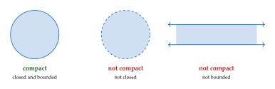
Key Idea.

In generative modelling, we often work with probability distributions on compact metric spaces. The Kantorovich–Rubinstein theorem (Proof of KR Duality in the Wasserstein GAN chapter) requires compactness to guarantee that the Wasserstein distance metrises weak convergence of probability measures. Compactness also underpins the Arzelà–Ascoli theorem, which controls the complexity of function classes used in discriminator and critic networks.

Remark 2 (Why Compactness Matters for Optimisation).

The extreme value theorem (which we prove in Extreme Value Theorem below) guarantees that a continuous function on a compact set attains its maximum and minimum. This is why many optimisation problems in machine learning implicitly assume compact parameter domains or add regularisation to effectively compactify the search space. Without compactness, a continuous objective can approach but never reach its infimum, and the “optimal” parameters may not exist.

Continuity

Continuity is the mathematical formalisation of the intuitive idea that “small changes in input produce small changes in output.” For generative modelling this concept is indispensable: the decoder of a variational autoencoder must map nearby latent codes to perceptually similar images, and the loss landscape that a GAN critic traverses must be sufficiently regular for gradient-based optimisation to succeed. In this section we develop the theory of continuity from the basic $ε$ - $δ$ definition through to the Lipschitz condition that underpins Wasserstein GANs.

Definitions of Continuity

Definition 18 ( $ε$ - $δ$ Continuity).

Let $(X, d_{X})$ and $(Y, d_{Y})$ be metric spaces. A function $f : X \to Y$ is continuous at a point $x_{0} \in X$ if for every $ε > 0$ there exists $δ > 0$ such that (EPS Delta) $\begin{matrix} d_{X} (x, x_{0}) < δ ⟹ d_{Y} (f (x), f (x_{0})) < ε . \end{matrix}$ The function $f$ is continuous on $X$ if it is continuous at every point of $X$ .

The definition says nothing about how large or small $δ$ must be in absolute terms; it only requires that a suitable $δ$ exists. Crucially, $δ$ may depend on both $ε$ and the point $x_{0}$ . When it depends only on $ε$ , we obtain the stronger notion of uniform continuity discussed in Uniform Continuity.

An equivalent and often more convenient characterisation uses sequences.

Theorem 12 (Sequential Characterisation).

Let $(X, d_{X})$ and $(Y, d_{Y})$ be metric spaces and let $f : X \to Y$ . Then $f$ is continuous at $x_{0} \in X$ if and only if for every sequence ${(x_{n})}_{n \geq 1}$ in $X$ with $x_{n} \to x_{0}$ , we have $f (x_{n}) \to f (x_{0})$ .

Proof.

$(\Rightarrow)$ ; Suppose $f$ is continuous at $x_{0}$ and let $(x_{n})$ be a sequence with $x_{n} \to x_{0}$ . Given $ε > 0$ , choose $δ > 0$ as in Definition 18. Since $x_{n} \to x_{0}$ , there exists $N$ such that $d_{X} (x_{n}, x_{0}) < δ$ for all $n \geq N$ . Then $d_{Y} (f (x_{n}), f (x_{0})) < ε$ for all $n \geq N$ , so $f (x_{n}) \to f (x_{0})$ .

$(\Leftarrow)$ ; We prove the contrapositive. Suppose $f$ is not continuous at $x_{0}$ . Then there exists $ε_{0} > 0$ such that for every $δ > 0$ there is a point $x$ with $d_{X} (x, x_{0}) < δ$ yet $d_{Y} (f (x), f (x_{0})) \geq ε_{0}$ . Taking $δ = 1 / n$ for $n = 1, 2, 3, \dots$ produces a sequence $(x_{n})$ with $x_{n} \to x_{0}$ but $d_{Y} (f (x_{n}), f (x_{0})) \geq ε_{0}$ for all $n$ , so $f (x_{n})$ does not converge to $f (x_{0})$ .

∎

Extreme Value Theorem

One of the most important consequences of continuity is that continuous functions on compact sets are guaranteed to attain their extreme values. Before stating the main result, we establish that continuous maps preserve compactness.

Theorem 13 (Continuous Image of a Compact Set).

Let $f : X \to Y$ be a continuous map between metric spaces. If $K \subseteq X$ is compact, then $f (K) \subseteq Y$ is compact.

Proof.

Let ${V_{α}}_{α \in A}$ be an open cover of $f (K)$ in $Y$ . For each $α$ , the preimage $U_{α} = f^{- 1} (V_{α})$ is open in $X$ because $f$ is continuous. Since every $y \in f (K)$ lies in some $V_{α}$ , every $x \in K$ lies in the corresponding $U_{α}$ , so ${U_{α}}_{α \in A}$ is an open cover of $K$ . By compactness of $K$ , there exists a finite subcover ${U_{α_{1}}, \dots, U_{α_{n}}}$ . Then ${V_{α_{1}}, \dots, V_{α_{n}}}$ covers $f (K)$ : for any $y = f (x) \in f (K)$ with $x \in K$ , we have $x \in U_{α_{i}}$ for some $i$ , hence $y \in V_{α_{i}}$ .

∎

Theorem 14 (Extreme Value Theorem).

If $f : K \to ℝ$ is continuous and $K$ is compact, then $f$ attains its maximum and minimum on $K$ . That is, there exist points $x_{\min}, x_{\max} \in K$ such that $f (x_{\min}) \leq f (x) \leq f (x_{\max}) for all x \in K .$

Proof.

By Theorem 13, $f (K)$ is a compact subset of $ℝ$ . The Heine–Borel theorem tells us that compact subsets of $ℝ$ are precisely the closed and bounded sets. Since $f (K)$ is bounded, $M = \sup f (K)$ and $m = \inf f (K)$ are finite. Since $f (K)$ is closed, both $M$ and $m$ belong to $f (K)$ . Therefore there exist $x_{\max} \in K$ with $f (x_{\max}) = M$ and $x_{\min} \in K$ with $f (x_{\min}) = m$ .

∎

The Extreme Value Theorem guarantees that a continuous function on a compact set attains both its maximum and minimum values. Here

f

achieves its maximum at

x_{\max}

and its minimum at

x_{\min}

within the closed interval

[a, b]

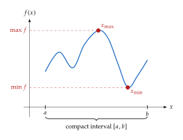
Uniform Continuity

Definition 19 (Uniform Continuity).

A function $f : X \to Y$ between metric spaces is uniformly continuous if for every $ε > 0$ there exists $δ > 0$ such that $d_{X} (x, y) < δ ⟹ d_{Y} (f (x), f (y)) < ε for 𝑎𝑙𝑙 x, y \in X .$

Remark 3 (Pointwise vs Uniform).

Ordinary continuity and uniform continuity differ in a subtle but important way. In the pointwise definition (Definition 18), $δ$ may depend on both $ε$ and the particular point $x_{0}$ . In the uniform definition, a single $δ$ works simultaneously for every pair of points in the domain. The distinction vanishes on compact domains, as the next theorem shows, but is significant on unbounded or non-closed domains.

Uniform vs. pointwise continuity. Left: The linear function

f (x) = x

is uniformly continuous because the same

δ

works at every point. Right: The function

f (x) = 1 / x

(0,1]

is continuous but not uniformly continuous: as

x

approaches

0

, the required

δ

for a fixed

ε

shrinks to zero.

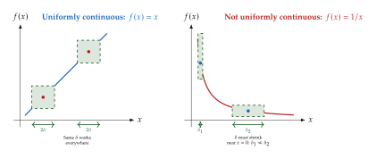
On compact domains, the distinction between pointwise and uniform continuity disappears. This classical result is essential in analysis and will be used repeatedly in later chapters.

Theorem 15 (Heine–Cantor).

Every continuous function on a compact metric space is uniformly continuous.

Proof.

Let $f : K \to Y$ be continuous on the compact metric space $K$ . Fix $ε > 0$ . For each $x \in K$ , continuity gives a $δ_{x} > 0$ such that $d_{X} (x, y) < δ_{x}$ implies $d_{Y} (f (x), f (y)) < ε / 2$ . The open balls ${B (x, δ_{x} / 2)}_{x \in K}$ cover $K$ . By compactness, finitely many suffice: $K \subseteq B (x_{1}, δ_{x_{1}} / 2) \cup \dots \cup B (x_{n}, δ_{x_{n}} / 2)$ . Set $δ = \frac{1}{2} \min {δ_{x_{1}}, \dots, δ_{x_{n}}} > 0$ .

Now suppose $d_{X} (y, z) < δ$ . Since the finite collection covers $K$ , there exists $x_{i}$ with $y \in B (x_{i}, δ_{x_{i}} / 2)$ . Then $d_{X} (z, x_{i}) \leq d_{X} (z, y) + d_{X} (y, x_{i}) < δ + \frac{δ_{x_{i}}}{2} \leq δ_{x_{i}} .$ Therefore $d_{Y} (f (y), f (x_{i})) < ε / 2$ and $d_{Y} (f (z), f (x_{i})) < ε / 2$ , so by the triangle inequality $d_{Y} (f (y), f (z)) < ε$ . Since $δ$ is independent of the choice of $y$ and $z$ , $f$ is uniformly continuous.

∎

Lipschitz Continuity

Uniform continuity guarantees a single $δ$ for each $ε$ , but says nothing about the rate at which the output changes with the input. Lipschitz continuity provides a quantitative bound on this rate, making it the strongest common continuity condition and the one most directly relevant to modern generative models.

Definition 20 (Lipschitz Continuity).

A function $f : X \to Y$ between metric spaces is $L$ -Lipschitz (or Lipschitz continuous with constant $L$ ) if there exists a constant $L \geq 0$ such that (Lipschitz) $\begin{matrix} d_{Y} (f (x), f (y)) \leq L \cdot d_{X} (x, y) for all x, y \in X . \end{matrix}$ The smallest such $L$ is called the Lipschitz constant of $f$ , denoted ${‖ f ‖}_{L}$ or $Lip (f)$ .

For differentiable functions, the Lipschitz constant has a clean gradient characterisation.

Definition 21 (Lipschitz Constant via Gradient).

Let $f : ℝ^{n} \to ℝ$ be differentiable. Then $f$ is $L$ -Lipschitz with respect to the Euclidean norm if and only if (Lipschitz GRAD) $\begin{matrix} ‖ \nabla f (𝒙) ‖ \leq L for all 𝒙 \in ℝ^{n} . \end{matrix}$

The various notions of continuity form a strict hierarchy.

Theorem 16 (Hierarchy of Continuity).

For functions between metric spaces, the following implications hold: $Lipschitz continuous ⟹ uniformly continuous ⟹ continuous .$ None of the converses hold in general.

Proof.

Lipschitz $\Rightarrow$ uniformly continuous.; If $f$ is $L$ -Lipschitz, set $δ = ε / L$ (or $δ = ε$ if $L = 0$ ). Then $d_{X} (x, y) < δ$ implies $d_{Y} (f (x), f (y)) \leq L \cdot d_{X} (x, y) < L \cdot (ε / L) = ε$ . This $δ$ is independent of the points $x$ and $y$ , so $f$ is uniformly continuous.

Uniformly continuous $\Rightarrow$ continuous.; Uniform continuity provides, for each $ε > 0$ , a single $δ > 0$ that works for all points. In particular it works at any fixed point $x_{0}$ , so $f$ is continuous at $x_{0}$ .

Converses fail.; The function $f (x) = \sqrt{x}$ on $[0,1]$ is uniformly continuous (it is continuous on a compact set, so the Heine–Cantor theorem applies) but not Lipschitz: its derivative $f^{'} (x) = 1 / (2 \sqrt{x})$ is unbounded as $x \to 0^{+}$ . The function $g (x) = x^{2}$ on $ℝ$ is continuous but not uniformly continuous: for $ε = 1$ , no single $δ$ works because $| {(x + δ / 2)}^{2} - {(x - δ / 2)}^{2} | = 2 x δ$ grows without bound as $x \to \infty$ .

∎

Example 9 (Lipschitz Functions).

Several common functions are Lipschitz continuous:

The linear function $f (x) = m x + b$ is $| m |$ -Lipschitz on $ℝ$ , since $| f (x) - f (y) | = | m | | x - y |$ .
The absolute value $f (x) = | x |$ is $1$ -Lipschitz, by the reverse triangle inequality.
The sine function $f (x) = \sin (x)$ is $1$ -Lipschitz, since $| \sin x - \sin y | \leq | x - y |$ by the mean value theorem and the bound $| \cos c | \leq 1$ .
The ReLU activation $f (x) = \max (0, x)$ is $1$ -Lipschitz.

Example 10 (Non-Lipschitz Functions).

Not every continuous function is Lipschitz:

$f (x) = x^{2}$ on $ℝ$ is not globally Lipschitz because $| f (x) - f (0) | / | x | = | x | \to \infty$ .
$f (x) = e^{x}$ on $ℝ$ fails to be Lipschitz for the same reason: its derivative grows without bound.
$f (x) = \sqrt{x}$ on $[0,1]$ is not Lipschitz because the derivative $1 / (2 \sqrt{x})$ blows up at $x = 0$ .

Key Idea.

In the Wasserstein GAN framework (10), the critic function is constrained to be $1$ -Lipschitz. This ensures that the Kantorovich–Rubinstein dual $W_{1} (P, Q) = \sup_{{‖ f ‖}_{L} \leq 1} [𝔼_{P} [f] - 𝔼_{Q} [f]]$ is finite and provides a meaningful distance between the real and generated distributions. Without the Lipschitz constraint, the supremum would diverge because the critic could become arbitrarily steep, driving the difference $𝔼_{P} [f] - 𝔼_{Q} [f]$ to infinity. In practice, the constraint is enforced by weight clipping, gradient penalty, or spectral normalisation.

Connectedness

Compactness captures the idea that a set is “small enough” to extract finite information from infinite data. Connectedness captures a different geometric property: the set is “in one piece.” A connected space cannot be split into two separate open chunks, and this topological rigidity has deep analytic consequences, the most famous being the Intermediate Value Theorem.

Definition 22 (Connected Set).

A metric space $(X, d)$ is connected if it cannot be written as a union $X = U \cup V$ of two nonempty, disjoint open sets $U$ and $V$ . Equivalently, $X$ is connected if and only if every continuous function $f : X \to {0, 1}$ is constant (where ${0,1}$ carries the discrete metric).

A stronger property requires that any two points can be joined by a continuous path.

Definition 23 (Path-Connected Set).

A metric space $X$ is path-connected if for every pair of points $x, y \in X$ there exists a continuous function $γ : [0,1] \to X$ with $γ (0) = x$ and $γ (1) = y$ . The function $γ$ is called a path from $x$ to $y$ .

Theorem 17 (Path-Connected Implies Connected).

Every path-connected metric space is connected.

Proof.

Suppose for contradiction that $X$ is path-connected but not connected. Then $X = U \cup V$ for nonempty disjoint open sets $U$ and $V$ . Pick $u \in U$ and $v \in V$ , and let $γ : [0,1] \to X$ be a path from $u$ to $v$ . The sets $γ^{- 1} (U)$ and $γ^{- 1} (V)$ are open in $[0,1]$ (since $γ$ is continuous and $U$ , $V$ are open), nonempty (since $0 \in γ^{- 1} (U)$ and $1 \in γ^{- 1} (V)$ ), disjoint, and their union is $[0,1]$ . But this contradicts the fact that the interval $[0,1]$ is connected.

∎

Remark 4 (The Converse Fails).

Path-connectedness is strictly stronger than connectedness. The classical counterexample is the topologist's sine curve: $S = {(x, \sin (1 / x)) : x > 0} \cup {(0, y) : - 1 \leq y \leq 1} .$ The set $S$ is connected (one cannot separate the oscillating part from the vertical segment without breaking continuity) but not path-connected: no continuous path can traverse the infinitely many oscillations near $x = 0$ in finite “time.”

Three subsets of

ℝ^{2}

. Left: A path-connected (hence connected) set with a path shown between two interior points. Middle: A disconnected set consisting of two separate components. Right: Two regions joined by a thin bridge remain connected.

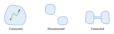
The most celebrated application of connectedness in elementary analysis is the Intermediate Value Theorem, which guarantees that continuous functions on intervals cannot “skip” values.

Theorem 18 (Intermediate Value Theorem).

Let $f : [a, b] \to ℝ$ be continuous. If $c$ is any real number strictly between $f (a)$ and $f (b)$ , then there exists $x^{*} \in (a, b)$ such that $f (x^{*}) = c$ .

Proof.

The interval $[a, b]$ is connected (it is path-connected, since the identity map provides a path between any two points). By Theorem 13 (with compactness replaced by the analogous result for connectedness: the continuous image of a connected set is connected), $f ([a, b])$ is a connected subset of $ℝ$ . The connected subsets of $ℝ$ are precisely the intervals. Since $f (a)$ and $f (b)$ both lie in $f ([a, b])$ , and $c$ lies between them, we have $c \in f ([a, b])$ . Therefore there exists $x^{*} \in [a, b]$ with $f (x^{*}) = c$ . Since $c$ is strictly between $f (a)$ and $f (b)$ , we have $x^{*} \neq a$ and $x^{*} \neq b$ , so $x^{*} \in (a, b)$ .

∎

Normed and Inner Product Spaces

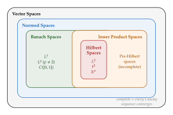
Metric spaces provide a general notion of distance, but in the vector spaces that arise throughout machine learning we have additional algebraic structure: vectors can be added and scaled. A norm measures the “size” of a vector in a way that respects this algebraic structure, while an inner product adds a notion of angle and orthogonality. The hierarchy $inner product spaces \subset normed spaces \subset metric spaces$ reflects increasing levels of geometric structure. Completeness then distinguishes Banach and Hilbert spaces as the settings where limits always exist, making calculus possible.

Normed Vector Spaces

Definition 24 (Norm).

Let $V$ be a vector space over $ℝ$ . A norm on $V$ is a function $‖ \cdot ‖ : V \to [0, \infty)$ satisfying, for all $𝒙, 𝒚 \in V$ and all $α \in ℝ$ :

Positive definiteness:; $‖ 𝒙 ‖ = 0$ if and only if $𝒙 = 𝟎$ .
Absolute homogeneity:; $‖ α 𝒙 ‖ = | α | ‖ 𝒙 ‖$ .
Triangle inequality:; $‖ 𝒙 + 𝒚 ‖ \leq ‖ 𝒙 ‖ + ‖ 𝒚 ‖$ .

Definition 25 (Normed Space).

A normed vector space (or simply a normed space) is a pair $(V, ‖ \cdot ‖)$ consisting of a vector space $V$ and a norm $‖ \cdot ‖$ on $V$ . Every normed space is automatically a metric space under the induced metric (Induced Metric) $\begin{matrix} d (𝒙, 𝒚) = ‖ 𝒙 - 𝒚 ‖ . \end{matrix}$

Example 11 ( $ℓ^{p}$ Norms on $ℝ^{n}$ ).

For $1 \leq p < \infty$ , the $ℓ^{p}$ norm on $ℝ^{n}$ is ${‖ 𝒙 ‖}_{p} = (\sum_{i = 1}^{n} {| x_{i} |}^{p})^{1 / p},$ and the $ℓ^{\infty}$ norm is ${‖ 𝒙 ‖}_{\infty} = \max_{1 \leq i \leq n} | x_{i} |$ . The most commonly used cases are $p = 1$ (Manhattan norm), $p = 2$ (Euclidean norm), and $p = \infty$ (maximum norm). The Euclidean norm $p = 2$ is special because it arises from an inner product.

$L^{p}$ Function Spaces

The $ℓ^{p}$ norms on $ℝ^{n}$ have infinite-dimensional counterparts that measure the “size” of functions rather than finite-dimensional vectors.

Definition 26 ( $L^{p}$ Space).

Let $(Ω, μ)$ be a measure space and let $1 \leq p < \infty$ . The space $L^{p} (Ω)$ consists of all (equivalence classes of) measurable functions $f : Ω \to ℝ$ for which ${‖ f ‖}_{p} = (\int_{Ω} {| f |}^{p} 𝖣 μ)^{1 / p} < \infty .$ For $p = \infty$ , the space $L^{\infty} (Ω)$ consists of essentially bounded functions with norm ${‖ f ‖}_{\infty} = {e s s s u p}_{x \in Ω} | f (x) |$ . Two functions that agree $μ$ -almost everywhere are identified.

Remark 5 (The Importance of $L^{2}$ ).

The space $L^{2}$ occupies a privileged position in the $L^{p}$ family: it is the only $L^{p}$ space that is a Hilbert space (every other, for $p \neq 2$ , is merely a Banach space). The inner product structure of $L^{2}$ gives access to the powerful geometry of orthogonal projections, Fourier analysis, and least-squares methods. In machine learning, the mean squared error loss $𝔼 [{‖ f (𝒙) - 𝒚 ‖}^{2}]$ is an $L^{2}$ quantity, and the reproducing kernel Hilbert spaces used in kernel methods are subspaces of $L^{2}$ .

Inner Product Spaces

Definition 27 (Inner Product Space).

Let $V$ be a vector space over $ℝ$ . An inner product on $V$ is a function $⟨ \cdot, \cdot ⟩ : V \times V \to ℝ$ satisfying, for all $𝒙, 𝒚, 𝒛 \in V$ and all $α \in ℝ$ :

Linearity in the first argument:; $⟨ α 𝒙 + 𝒚, 𝒛 ⟩ = α ⟨ 𝒙, 𝒛 ⟩ + ⟨ 𝒚, 𝒛 ⟩$ .
Symmetry:; $⟨ 𝒙, 𝒚 ⟩ = ⟨ 𝒚, 𝒙 ⟩$ .
Positive definiteness:; $⟨ 𝒙, 𝒙 ⟩ \geq 0$ , with equality if and only if $𝒙 = 𝟎$ .

Every inner product induces a norm via $‖ 𝒙 ‖ = \sqrt{⟨ 𝒙, 𝒙 ⟩}$ , and hence a metric via $d (𝒙, 𝒚) = ‖ 𝒙 - 𝒚 ‖$ .

The fundamental inequality of inner product spaces relates the inner product to the induced norm.

Theorem 19 (Cauchy–Schwarz Inequality).

For any $𝒙, 𝒚$ in an inner product space $V$ , (Cauchy Schwarz) $\begin{matrix} | ⟨ 𝒙, 𝒚 ⟩ | \leq ‖ 𝒙 ‖ ‖ 𝒚 ‖ . \end{matrix}$ Equality holds if and only if $𝒙$ and $𝒚$ are linearly dependent.

Proof.

If $𝒚 = 𝟎$ , both sides are zero and the inequality holds trivially. Assume $𝒚 \neq 𝟎$ and consider the function $g (t) = {‖ 𝒙 + t 𝒚 ‖}^{2} = ⟨ 𝒙 + t 𝒚, 𝒙 + t 𝒚 ⟩ = {‖ 𝒙 ‖}^{2} + 2 t ⟨ 𝒙, 𝒚 ⟩ + t^{2} {‖ 𝒚 ‖}^{2} .$ By positive definiteness of the inner product, $g (t) \geq 0$ for all $t \in ℝ$ . This is a non-negative quadratic polynomial in $t$ , so its discriminant must satisfy $(2 ⟨ 𝒙, 𝒚 ⟩)^{2} - 4 {‖ 𝒙 ‖}^{2} {‖ 𝒚 ‖}^{2} \leq 0,$ which simplifies to ${⟨ 𝒙, 𝒚 ⟩}^{2} \leq {‖ 𝒙 ‖}^{2} {‖ 𝒚 ‖}^{2}$ . Taking square roots gives the result. Equality holds precisely when $g (t) = 0$ for some $t$ , which means $𝒙 + t 𝒚 = 𝟎$ , so $𝒙$ and $𝒚$ are linearly dependent.

∎

Banach and Hilbert Spaces

The spaces $ℝ^{n}$ are “well-behaved” because every Cauchy sequence converges. In infinite-dimensional settings this completeness property must be imposed as an axiom, leading to the central objects of functional analysis.

Definition 28 (Banach Space).

A normed vector space $(V, ‖ \cdot ‖)$ is a Banach space if it is complete: every Cauchy sequence in $V$ converges to a limit in $V$ .

Definition 29 (Hilbert Space).

An inner product space $(V, ⟨ \cdot, \cdot ⟩)$ is a Hilbert space if it is complete with respect to the norm induced by the inner product.

Every Hilbert space is a Banach space (the inner product induces a norm, and completeness is assumed), but a Banach space need not be a Hilbert space because its norm may not arise from any inner product. A classical test is the parallelogram law: a norm $‖ \cdot ‖$ comes from an inner product if and only if ${‖ 𝒙 + 𝒚 ‖}^{2} + {‖ 𝒙 - 𝒚 ‖}^{2} = 2 {‖ 𝒙 ‖}^{2} + 2 {‖ 𝒚 ‖}^{2}$ for all $𝒙, 𝒚$ .

Example 12 ( $L^{2}$ as a Hilbert Space).

The space $L^{2} ([0,1])$ with the inner product $⟨ f, g ⟩ = \int_{0}^{1} f (x) g (x) 𝖣 x$ is a Hilbert space. The induced norm is ${‖ f ‖}_{2} = {(\int_{0}^{1} {| f (x) |}^{2} 𝖣 x)}^{1 / 2}$ , and completeness follows from the Riesz–Fischer theorem. Fourier series provide orthonormal bases for $L^{2}$ , making it the natural home for spectral analysis.

Example 13 ( $L^{1}$ as a Banach Space (not Hilbert)).

The space $L^{1} ([0,1])$ with norm ${‖ f ‖}_{1} = \int_{0}^{1} | f (x) | 𝖣 x$ is a Banach space (complete) but not a Hilbert space. Its norm fails the parallelogram law, so no inner product can generate it. This means $L^{1}$ lacks the orthogonal projection machinery that makes $L^{2}$ so tractable.

A cornerstone result connects continuous linear functionals on a Hilbert space to elements of the space itself.

Theorem 20 (Riesz Representation).

Let $H$ be a Hilbert space over $ℝ$ . For every continuous linear functional $φ : H \to ℝ$ , there exists a unique element $g \in H$ such that (Riesz) $\begin{matrix} φ (f) = ⟨ f, g ⟩ for all f \in H . \end{matrix}$ Moreover, $‖ φ ‖ = ‖ g ‖$ .

The intuition behind the Riesz Representation Theorem is striking: every “measurement” that you can perform on elements of a Hilbert space (that is, every continuous linear functional) amounts to taking an inner product with some fixed element of the space. There are no “exotic” linear functionals lurking beyond the inner product structure. This makes Hilbert spaces exceptionally well-suited for optimisation and approximation theory, since searching over functionals reduces to searching over elements of the space itself.

The hierarchy of vector spaces used in analysis and machine learning. Every Hilbert space is both a Banach space (complete normed space) and an inner product space. The

L^{p}

spaces for

p \neq 2

are Banach but not Hilbert, while incomplete inner product spaces (sometimes called pre-Hilbert spaces) are neither Banach nor Hilbert.

Topology

Every metric space carries a natural notion of “open set,” and it is this collection of open sets, rather than the metric itself, that determines which functions are continuous, which sets are compact, and which sequences converge. Topology abstracts this observation: it studies the properties of spaces that depend only on the open-set structure. For generative modelling the key payoff is the distinction between strong and weak topologies, which explains why the Wasserstein distance succeeds where the KL divergence fails.

Topological Spaces

Definition 30 (Topological Space).

A topological space is a pair $(X, 𝒯)$ , where $X$ is a set and $𝒯 \subseteq 𝒫 (X)$ is a collection of subsets of $X$ called open sets, satisfying:

The empty set $\emptyset$ and the whole space $X$ belong to $𝒯$ .
The intersection of any finite collection of members of $𝒯$ belongs to $𝒯$ .
The union of any (possibly infinite) collection of members of $𝒯$ belongs to $𝒯$ .

These three axioms are deliberately minimal: they capture the essential algebraic properties of open sets in metric spaces while discarding the specific notion of distance. A closed set in a topological space is, by definition, the complement of an open set.

Definition 31 (Basis for a Topology).

A collection $ℬ \subseteq 𝒯$ of open sets is a basis for the topology $𝒯$ if every open set in $𝒯$ can be written as a (possibly empty) union of members of $ℬ$ .

Remark 6 (Metric Topology).

Every metric space $(X, d)$ has a natural topology: the collection of all sets $U \subseteq X$ such that for every $x \in U$ there exists $ε > 0$ with $B (x, ε) \subseteq U$ . The open balls ${B (x, ε) : x \in X, ε > 0}$ form a basis for this topology. This construction provides the bridge between the concrete metric framework of Continuity and the abstract topological viewpoint developed here. Two different metrics on the same set can generate the same topology (they are then called topologically equivalent), which is why topological properties are more fundamental than metric ones.

Strong and Weak Topologies

In finite-dimensional spaces such as $ℝ^{n}$ , there is essentially only one “reasonable” topology (all norms on $ℝ^{n}$ are equivalent). In infinite-dimensional spaces the situation is dramatically different: the same underlying set can carry multiple topologies that lead to genuinely different notions of convergence. The two most important are the strong (norm) topology and the weak topology.

The strong topology (also called the norm topology) on a normed space $(V, ‖ \cdot ‖)$ is simply the metric topology induced by the norm. A sequence $(𝒙_{n})$ converges strongly to $𝒙$ if $‖ 𝒙_{n} - 𝒙 ‖ \to 0$ . This is the most natural and demanding form of convergence.

Definition 32 (Weak Topology).

Let $(V, ‖ \cdot ‖)$ be a normed space and let $V^{*}$ denote its dual space (the set of all continuous linear functionals $φ : V \to ℝ$ ). The weak topology on $V$ is the coarsest topology that makes every $φ \in V^{*}$ continuous. Concretely, a set $U \subseteq V$ is open in the weak topology if and only if for every $𝒙 \in U$ there exist finitely many functionals $φ_{1}, \dots, φ_{k} \in V^{*}$ and $ε > 0$ such that ${𝒚 \in V : | φ_{i} (𝒚) - φ_{i} (𝒙) | < ε for all i = 1, \dots, k} \subseteq U .$

Definition 33 (Weak Convergence).

A sequence $(𝒙_{n})$ in a normed space $V$ converges weakly to $𝒙 \in V$ , written $𝒙_{n} ⇀ 𝒙$ , if $φ (𝒙_{n}) \to φ (𝒙) for every φ \in V^{*} .$ That is, $𝒙_{n} ⇀ 𝒙$ if and only if $𝒙_{n} \to 𝒙$ in the weak topology.

The weak topology has fewer open sets than the strong topology (it is “coarser”), so it is easier for a sequence to converge weakly than strongly.

Theorem 21 (Strong Implies Weak).

If $𝒙_{n} \to 𝒙$ in norm (strong convergence), then $𝒙_{n} ⇀ 𝒙$ (weak convergence). The converse holds in finite-dimensional spaces but fails in infinite-dimensional ones.

Proof.

Suppose $‖ 𝒙_{n} - 𝒙 ‖ \to 0$ and let $φ \in V^{*}$ be any continuous linear functional. By linearity and continuity, $| φ (𝒙_{n}) - φ (𝒙) | = | φ (𝒙_{n} - 𝒙) | \leq ‖ φ ‖ ‖ 𝒙_{n} - 𝒙 ‖ \to 0,$ where $‖ φ ‖ = \sup_{‖ 𝒚 ‖ \leq 1} | φ (𝒚) |$ is the operator norm. Therefore $φ (𝒙_{n}) \to φ (𝒙)$ for every $φ \in V^{*}$ , which is exactly weak convergence.

∎

Theorem 22 (Equivalence in Finite Dimensions).

In a finite-dimensional normed space, weak convergence and strong convergence are equivalent.

Proof sketch.

Let $V = ℝ^{n}$ with any norm. Every continuous linear functional on $ℝ^{n}$ has the form $φ (𝒙) = 𝐚^{⊤} 𝒙$ for some $𝐚 \in ℝ^{n}$ . Suppose $𝒙_{n} ⇀ 𝒙$ , so $𝐚^{⊤} 𝒙_{n} \to 𝐚^{⊤} 𝒙$ for all $𝐚 \in ℝ^{n}$ . Choosing $𝐚 = 𝐞_{i}$ (the $i$ -th standard basis vector) shows that each component converges: ${(𝒙_{n})}_{i} \to {(𝒙)}_{i}$ . Componentwise convergence in $ℝ^{n}$ implies convergence in norm (since all norms on $ℝ^{n}$ are equivalent), so $𝒙_{n} \to 𝒙$ strongly.

∎

The following example shows that in infinite dimensions the equivalence breaks down.

Example 14 (Weak But Not Strong Convergence).

In $L^{2} ([0,1])$ , define $f_{n} (x) = \sqrt{2} \sin (n π x), n = 1, 2, 3, \dots$ Each $f_{n}$ has unit norm: ${‖ f_{n} ‖}_{2} = 1$ . By the Riemann–Lebesgue lemma, for any $g \in L^{2} ([0,1])$ , $⟨ f_{n}, g ⟩ = \sqrt{2} \int_{0}^{1} \sin (n π x) g (x) 𝖣 x \to 0 as n \to \infty .$ Therefore $f_{n} ⇀ 0$ weakly. However, ${‖ f_{n} - 0 ‖}_{2} = 1$ for all $n$ , so the sequence does not converge strongly to $0$ . The oscillations become ever more rapid but never diminish in amplitude.

Key Idea.

In generative modelling, we compare probability distributions, which live in infinite-dimensional function spaces. The KL divergence induces strong-topology-like behaviour: it can be infinite even when distributions are “close” in a perceptually meaningful sense (for instance, when the supports are disjoint but nearby). The Wasserstein distance, by contrast, metrises weak convergence on compact spaces: $W_{p} (μ_{n}, μ) \to 0$ if and only if $μ_{n}$ converges weakly to $μ$ (and the $p$ -th moments converge). This means the Wasserstein distance captures the intuitive notion that a sequence of distributions $P_{n}$ approaches $P$ when samples from $P_{n}$ “look like” samples from $P$ . It is precisely this property that makes the Wasserstein distance preferable to the KL divergence as a training objective in WGANs: the loss landscape is smooth even when the generator's distribution has not yet “found” the data manifold.

Historical Note.

The distinction between weak and strong convergence was first systematically studied by Stefan Banach and his Lwów school in the 1920s and 1930s. Their insights, recorded in the famous Scottish Book of open problems kept in a Lwów café, laid the foundations of modern functional analysis. Banach's 1932 monograph Théorie des opérations linéaires introduced many of the concepts discussed in this section, including the systematic use of dual spaces and weak convergence.

For generative modelling, weak convergence became directly relevant when Arjovsky, Chintala, and Bottou (2017) showed that the Wasserstein distance provides meaningful gradients where the KL divergence and Jensen–Shannon divergence fail. Their paper demonstrated that sequences of distributions approaching the data distribution may have infinite KL divergence at every step, while the Wasserstein distance decreases smoothly, a phenomenon explained precisely by the difference between strong and weak topologies.

Differentiation and Integration in $ℝ^{n}$

The tools of multivariable calculus form the computational backbone of modern generative modelling. Gradients drive optimisation, Jacobians govern how densities transform under invertible maps, and integration by parts is the hidden engine behind score matching. In this section we develop these tools with enough precision to support the theoretical results used throughout the main text, while keeping an eye on the practical consequences for model design and training. Readers comfortable with undergraduate multivariable calculus will find most of this material a review, but the connections to generative modelling should be fresh.

Gradients, Jacobians, and Hessians

We begin with the three fundamental derivative objects of multivariable calculus. The gradient $\nabla f$ captures first-order information about scalar-valued functions, the Jacobian $J_{F}$ generalises this to vector-valued maps, and the Hessian $H_{f}$ captures second-order (curvature) information. Each appears repeatedly in the design and analysis of generative models, and understanding their interplay is essential for the developments in subsequent chapters.

Definition 34 (Gradient).

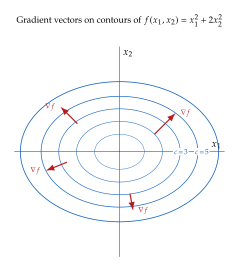
Let $f : ℝ^{n} \to ℝ$ be differentiable at $𝒙 \in ℝ^{n}$ . The gradient of $f$ at $𝒙$ is the column vector of first partial derivatives: (Gradient) $\begin{matrix} \nabla f (𝒙) = (\begin{matrix} \frac{\partial f}{\partial x_{1}} (𝒙) \\ ⋮ \\ \frac{\partial f}{\partial x_{n}} (𝒙) \end{matrix}) \in ℝ^{n} . \end{matrix}$ The gradient points in the direction of steepest ascent of $f$ at $𝒙$ , and its magnitude $‖ \nabla f (𝒙) ‖$ equals the maximum directional derivative.

The gradient is the workhorse of gradient-based optimisation: every step of stochastic gradient descent moves the parameters in the direction $- \nabla_{θ} ℒ (θ)$ , and the score function $\nabla_{𝒙} \log p (𝒙)$ that drives diffusion models and score matching is simply the gradient of the log-density with respect to data.

Example 15 (Gradient of a Quadratic).

For the quadratic function $f (𝒙) = \frac{1}{2} 𝒙^{⊤} A 𝒙 + 𝒃^{⊤} 𝒙 + c$ where $A$ is a symmetric matrix, $𝒃 \in ℝ^{n}$ , and $c \in ℝ$ , the gradient is $\nabla f (𝒙) = A 𝒙 + 𝒃$ . Setting the gradient to zero gives the critical point $𝒙^{*} = - A^{- 1} 𝒃$ (when $A$ is invertible). This is the solution to a linear system and appears throughout machine learning in closed-form solutions for linear regression and Gaussian conditioning.

Definition 35 (Jacobian Matrix).

Let $F : ℝ^{n} \to ℝ^{m}$ be differentiable at $𝒙$ . The Jacobian matrix of $F$ at $𝒙$ is the $m \times n$ matrix (Jacobian) $\begin{matrix} J_{F} (𝒙) = (\begin{matrix} \frac{\partial F_{1}}{\partial x_{1}} & \dots & \frac{\partial F_{1}}{\partial x_{n}} \\ ⋮ & ⋱ & ⋮ \\ \frac{\partial F_{m}}{\partial x_{1}} & \dots & \frac{\partial F_{m}}{\partial x_{n}} \end{matrix}), \end{matrix}$ so that ${(J_{F} (𝒙))}_{i j} = \partial F_{i} / \partial x_{j}$ . The Jacobian provides the best linear approximation to $F$ near $𝒙$ : $\begin{matrix} F (𝒙 + 𝒉) = F (𝒙) + J_{F} (𝒙) 𝒉 + o (‖ 𝒉 ‖) . \end{matrix}$ When $m = 1$ , the Jacobian reduces to the transpose of the gradient: $J_{f} (𝒙) = {(\nabla f (𝒙))}^{⊤}$ .

Example 16 (Jacobian of an Affine Map).

The affine map $F (𝒙) = A 𝒙 + 𝒃$ , where $A \in ℝ^{m \times n}$ and $𝒃 \in ℝ^{m}$ , has constant Jacobian $J_{F} (𝒙) = A$ . This is the simplest non-trivial example and already illustrates the key principle: the determinant $| \det A |$ measures how the linear map stretches volume. For a square matrix ( $m = n$ ), if $| \det A | > 1$ the map expands volumes, and if $| \det A | < 1$ it compresses them. Normalizing flow layers often compose such simple maps to build expressive transformations while keeping the Jacobian determinant tractable.

Definition 36 (Hessian Matrix).

Let $f : ℝ^{n} \to ℝ$ be twice differentiable at $𝒙$ . The Hessian matrix of $f$ at $𝒙$ is the $n \times n$ matrix of second partial derivatives: (Hessian) $\begin{matrix} H_{f} (𝒙) = \nabla^{2} f (𝒙), {(H_{f} (𝒙))}_{i j} = \frac{\partial^{2} f}{\partial x_{i} \partial x_{j}} (𝒙) . \end{matrix}$ If $f \in C^{2}$ (all second partial derivatives exist and are continuous), then $H_{f} (𝒙)$ is symmetric by Schwarz's theorem (also known as Clairaut's theorem): $\begin{matrix} \frac{\partial^{2} f}{\partial x_{i} \partial x_{j}} = \frac{\partial^{2} f}{\partial x_{j} \partial x_{i}} . \end{matrix}$ The Hessian encodes the local curvature of $f$ . At a critical point where $\nabla f = 0$ , the eigenvalues of $H_{f}$ determine whether the point is a local minimum (all positive), local maximum (all negative), or saddle point (mixed signs).

Example 17 (Hessian of the Log-Gaussian).

For the multivariate Gaussian log-density $\log p (𝒙) = - \frac{1}{2} {(𝒙 - 𝝁)}^{⊤} Σ^{- 1} (𝒙 - 𝝁) + const$ , the gradient (score) is $\nabla_{𝒙} \log p (𝒙) = - Σ^{- 1} (𝒙 - 𝝁)$ and the Hessian is $\nabla_{𝒙}^{2} \log p (𝒙) = - Σ^{- 1}$ , a constant matrix. This is one of the few cases where the Hessian is independent of $𝒙$ , reflecting the fact that a Gaussian has uniform curvature. The trace of the Hessian is $trace (- Σ^{- 1}) = - \sum_{i = 1}^{n} 1 / σ_{i}^{2}$ , where $σ_{i}^{2}$ are the eigenvalues of $Σ$ .

Gradient vectors (red arrows) on the contour plot of

f (x_{1}, x_{2}) = x_{1}^{2} + 2 x_{2}^{2}

. The gradient is always perpendicular to the level curves, and its magnitude is larger where contours are closer together (steeper regions).

Insight.

The chain rule in multiple dimensions states that $J_{G \circ F} (𝒙) = J_{G} (F (𝒙)) \cdot J_{F} (𝒙)$ . Taking determinants gives $\det J_{G \circ F} = \det J_{G} \cdot \det J_{F}$ . For normalizing flows that compose $K$ invertible layers $Φ = Φ_{K} \circ \dots \circ Φ_{1}$ , this factorisation means $\log | \det J_{Φ} | = \sum_{k = 1}^{K} \log | \det J_{Φ_{k}} |$ . Each layer contributes an additive term to the log-determinant, which is why composing simple layers with cheap determinants produces an expressive flow with a tractable density.

Definition 37 (Trace).

For a square matrix $A \in ℝ^{n \times n}$ , the trace is the sum of its diagonal entries: (Trace DEF) $\begin{matrix} trace (A) = \sum_{i = 1}^{n} A_{i i} . \end{matrix}$

Theorem 23 (Trace Properties).

Let $A, B, C$ be matrices of compatible dimensions and $α \in ℝ$ . Then:

Linearity: $trace (A + α B) = trace (A) + α trace (B)$ .
Transpose invariance: $trace (A^{⊤}) = trace (A)$ .
Cyclic property: $trace (A B C) = trace (B C A) = trace (C A B)$ .
Eigenvalue relation: If $λ_{1}, \dots, λ_{n}$ are the eigenvalues of $A$ (counted with algebraic multiplicity), then $trace (A) = \sum_{i = 1}^{n} λ_{i}$ .

Proof.

Properties (i) and (ii) follow directly from the definition. For the cyclic property, let $A \in ℝ^{m \times p}$ , $B \in ℝ^{p \times q}$ , $C \in ℝ^{q \times m}$ . Then (Cyclic Proof) $\begin{matrix} trace (A B C) & = \sum_{i = 1}^{m} {(A B C)}_{i i} = \sum_{i = 1}^{m} \sum_{j = 1}^{p} \sum_{k = 1}^{q} A_{i j} B_{j k} C_{k i} \\ = \sum_{j = 1}^{p} \sum_{k = 1}^{q} \sum_{i = 1}^{m} B_{j k} C_{k i} A_{i j} = \sum_{j = 1}^{p} {(B C A)}_{j j} = trace (B C A) . \end{matrix}$ The second equality $trace (B C A) = trace (C A B)$ follows by applying the same argument to the product $B C A$ . Property (iv) follows from the fact that similar matrices share the same trace, and every matrix is similar (over $ℂ$ ) to its Jordan normal form, whose diagonal entries are the eigenvalues.

∎

The cyclic property of the trace is surprisingly powerful. It allows us to convert scalar expressions into matrix forms and vice versa: for instance, the quadratic form $𝒙^{⊤} A 𝒙$ can be written as $trace (A 𝒙 𝒙^{⊤})$ , a rewriting that underlies the next result.

Definition 38 (Hutchinson's Trace Estimator).

For any square matrix $A \in ℝ^{n \times n}$ , the trace can be expressed as the expectation (Hutchinson) $\begin{matrix} trace (A) = 𝔼 [𝒗^{⊤} A 𝒗], \end{matrix}$ where $𝒗$ is a random vector satisfying $𝔼 [𝒗] = 0$ and $𝔼 [𝒗 𝒗^{⊤}] = I$ . Common choices for the distribution of $𝒗$ include Rademacher random vectors (each entry independently $\pm 1$ with equal probability) and standard Gaussian vectors.

Proof.

Using the cyclic property of the trace and the linearity of expectation: $\begin{matrix} 𝔼 [𝒗^{⊤} A 𝒗] = 𝔼 [trace (𝒗^{⊤} A 𝒗)] = 𝔼 [trace (A 𝒗 𝒗^{⊤})] = trace (A 𝔼 [𝒗 𝒗^{⊤}]) = trace (A \cdot I) = trace (A) . \end{matrix}$ The key step is interchanging $trace$ and $𝔼$ , which is justified by the linearity of both operators.

∎

The variance of the estimator depends on the distribution of $𝒗$ and the structure of $A$ . For Rademacher vectors, $𝖵ar (𝒗^{⊤} A 𝒗) = 2 {‖ A ‖}_{F}^{2} - 2 \sum_{i} A_{i i}^{2}$ , where ${‖ A ‖}_{F}$ is the Frobenius norm. Gaussian probe vectors give higher variance, $𝖵ar = 2 {‖ A ‖}_{F}^{2}$ , but are easier to generate. In practice, a small number of random projections (often just one per training step) provides sufficient gradient signal.

Remark 7 (Hutchinson's Estimator and Score Matching).

Hutchinson's estimator is the computational trick that makes sliced score matching practical. In score matching, one must evaluate $trace (\nabla_{𝒙}^{2} \log p_{θ} (𝒙))$ , which naively requires $O (n)$ backward passes through the network (one per diagonal entry of the Hessian). Hutchinson's estimator replaces this with a single random projection $𝒗$ , yielding the unbiased estimate $𝒗^{⊤} \nabla_{𝒙}^{2} \log p_{θ} (𝒙) 𝒗$ , computable with just one forward-backward pass via the identity $𝒗^{⊤} \nabla^{2} f \cdot 𝒗 = 𝒗^{⊤} \nabla (\nabla f \cdot 𝒗)$ . This reduces the cost from $O (n)$ to $O (1)$ backward passes per sample.

Integration by Parts

Integration by parts transfers a derivative from one factor of an integrand to another. This seemingly modest operation is the single most important analytical tool in the theory of score matching. We first state the familiar one-dimensional version and then extend it to $ℝ^{n}$ , where it takes on the form of the divergence theorem.

Theorem 24 (Integration by Parts (One Dimension)).

If $f$ and $g$ are continuously differentiable on $[a, b]$ , then (IBP 1D) $\begin{matrix} \int_{a}^{b} f (x) g^{'} (x) d x = [f (x) g (x)]_{a}^{b} - \int_{a}^{b} f^{'} (x) g (x) d x . \end{matrix}$

Proof.

The product rule gives ${(f g)}^{'} = f^{'} g + f g^{'}$ , so $f g^{'} = {(f g)}^{'} - f^{'} g$ . Integrating both sides over $[a, b]$ and applying the fundamental theorem of calculus to the first term yields $\int_{a}^{b} f g^{'} d x = \int_{a}^{b} (f g)^{'} d x - \int_{a}^{b} f^{'} g d x = [f g]_{a}^{b} - \int_{a}^{b} f^{'} g d x .$

∎

Theorem 25 (Multivariate Integration by Parts).

Let $𝒇 : ℝ^{n} \to ℝ^{n}$ be a continuously differentiable vector field and $g : ℝ^{n} \to ℝ$ a continuously differentiable function. If $g (𝒙) 𝒇 (𝒙) \to 0$ as $‖ 𝒙 ‖ \to \infty$ , then (IBP Multi) $\begin{matrix} \int_{ℝ^{n}} g (𝒙) (\nabla \cdot 𝒇) (𝒙) d 𝒙 = - \int_{ℝ^{n}} {(\nabla g (𝒙))}^{⊤} 𝒇 (𝒙) d 𝒙, \end{matrix}$ where $\nabla \cdot 𝒇 = \sum_{i = 1}^{n} \partial f_{i} / \partial x_{i}$ is the divergence of $𝒇$ .

Proof.

We apply the one-dimensional integration by parts formula to each coordinate. For the $i$ -th component, integrating with respect to $x_{i}$ while holding all other variables fixed: $\int_{- \infty}^{\infty} g (𝒙) \frac{\partial f_{i}}{\partial x_{i}} (𝒙) d x_{i} = [g (𝒙) f_{i} (𝒙)]_{x_{i} = - \infty}^{x_{i} = \infty} - \int_{- \infty}^{\infty} \frac{\partial g}{\partial x_{i}} (𝒙) f_{i} (𝒙) d x_{i} .$ The boundary term $[g f_{i}]$ vanishes by the decay assumption $g (𝒙) 𝒇 (𝒙) \to 0$ as $‖ 𝒙 ‖ \to \infty$ . Summing over $i = 1, \dots, n$ and integrating over all remaining variables gives $\int_{ℝ^{n}} g (\nabla \cdot 𝒇) d 𝒙 = - \sum_{i = 1}^{n} \int_{ℝ^{n}} \frac{\partial g}{\partial x_{i}} f_{i} d 𝒙 = - \int_{ℝ^{n}} {(\nabla g)}^{⊤} 𝒇 d 𝒙 .$

∎

Key Idea.

Integration by parts is the fundamental tool behind score matching. Hyvärinen's key insight was to apply integration by parts to the Fisher divergence $𝔼_{p_{d}} [{‖ \nabla_{𝒙} \log p_{θ} (𝒙) - \nabla_{𝒙} \log p_{d} (𝒙) ‖}^{2}],$ which appears intractable because it involves the unknown data score $\nabla_{𝒙} \log p_{d}$ . By expanding the square and integrating by parts, the cross-term $𝔼_{p_{d}} [{(\nabla \log p_{d})}^{⊤} (\nabla \log p_{θ})]$ can be rewritten in terms of $trace (\nabla^{2} \log p_{θ})$ and $\nabla \log p_{θ}$ alone. The derivative is effectively “transferred” from the unknown $p_{d}$ onto the known model $p_{θ}$ . The boundary terms vanish precisely because probability densities decay to zero at infinity.

Change of Variables

The change-of-variables formula describes how integrals transform under smooth, invertible coordinate changes. It is the mathematical bedrock upon which normalizing flows are built. The basic intuition is straightforward: when we “stretch” or “compress” a region of space through a smooth map, volumes change by a factor determined by the Jacobian determinant. For probability densities, which must integrate to one, this volume factor appears as a correction term that ensures the transformed density remains properly normalised.

Theorem 26 (Change of Variables (One Dimension)).

If $φ : [a, b] \to [c, d]$ is a $C^{1}$ diffeomorphism (smooth bijection with smooth inverse), then for any integrable function $f$ , (COV 1D) $\begin{matrix} \int_{c}^{d} f (y) d y = \int_{a}^{b} f (φ (x)) | φ^{'} (x) | d x . \end{matrix}$ The absolute value $| φ^{'} (x) |$ accounts for the possibility that $φ$ reverses orientation (i.e., is decreasing).

Proof.

If $φ$ is increasing, then $φ^{'} > 0$ and the result follows directly from the substitution $y = φ (x)$ , $d y = φ^{'} (x) d x$ . If $φ$ is decreasing, then $φ^{'} < 0$ and the substitution reverses the limits of integration. The two sign changes (from $φ^{'} < 0$ and from reversing limits) cancel, yielding the absolute value.

∎

Theorem 27 (Change of Variables (Multivariate)).

Let $Φ : U \to V$ be a $C^{1}$ diffeomorphism between open subsets $U, V \subseteq ℝ^{n}$ . Then for any integrable function $f : V \to ℝ$ , (COV Multi) $\begin{matrix} \int_{V} f (𝒚) d 𝒚 = \int_{U} f (Φ (𝒙)) | \det J_{Φ} (𝒙) | d 𝒙, \end{matrix}$ where $J_{Φ}$ is the $n \times n$ Jacobian matrix of $Φ$ .

The factor $| \det J_{Φ} (𝒙) |$ measures how $Φ$ locally stretches or compresses volume. If $Φ$ doubles all lengths, the determinant is $2^{n}$ and the volume element is scaled accordingly.

Proof sketch of Theorem 27.

The idea is to approximate $Φ$ locally by its linear part. Partition $U$ into small cubes $Q_{k}$ of side length $δ$ . On each cube, $Φ$ is approximately affine: $Φ (𝒙) \approx Φ (𝒙_{k}) + J_{Φ} (𝒙_{k}) (𝒙 - 𝒙_{k})$ for some centre point $𝒙_{k} \in Q_{k}$ . The image $Φ (Q_{k})$ is approximately a parallelepiped whose volume is $| \det J_{Φ} (𝒙_{k}) | \cdot δ^{n}$ . Thus $\int_{V} f (𝒚) d 𝒚 \approx \sum_{k} f (Φ (𝒙_{k})) | \det J_{Φ} (𝒙_{k}) | δ^{n} \approx \int_{U} f (Φ (𝒙)) | \det J_{Φ} (𝒙) | d 𝒙 .$ Making this approximation rigorous requires showing that the error vanishes as $δ \to 0$ , which uses the differentiability of $Φ$ and standard measure-theoretic arguments. The full proof can be found in any graduate real analysis text.

∎

Example 18 (Polar Coordinates).

Define $Φ (r, θ) = (r \cos θ, r \sin θ)$ for $r > 0$ , $θ \in (0, 2 π)$ . The Jacobian is $J_{Φ} = (\begin{matrix} \cos θ & - r \sin θ \\ \sin θ & r \cos θ \end{matrix}), \det J_{Φ} = r .$ The change-of-variables formula gives $\int_{ℝ^{2}} f (𝒙) d 𝒙 = \int_{0}^{\infty} \int_{0}^{2 π} f (r \cos θ, r \sin θ) r d θ d r$ , recovering the familiar area element $r d r d θ$ in polar coordinates. This conversion is used throughout probability to compute expectations of radially symmetric densities, including the Gaussian integral.

Key Idea.

The change-of-variables formula is the mathematical foundation of normalizing flows. A normalizing flow transforms a simple base density $p_{Z} (𝒛)$ (typically a standard Gaussian) through an invertible map $Φ$ to produce a complex target density. If $𝒙 = Φ (𝒛)$ , the density of $𝒙$ is $p_{X} (𝒙) = p_{Z} (Φ^{- 1} (𝒙)) | \det J_{Φ^{- 1}} (𝒙) | .$ Taking logarithms, $\log p_{X} (𝒙) = \log p_{Z} (Φ^{- 1} (𝒙)) - \log | \det J_{Φ} (Φ^{- 1} (𝒙)) |$ . Training requires evaluating $\log | \det J_{Φ} |$ , which costs $O (n^{3})$ for a dense Jacobian. This motivates flow architectures with structured Jacobians: autoregressive flows and coupling layers have triangular Jacobians, reducing the determinant computation to $O (n)$ (since the determinant of a triangular matrix is just the product of its diagonal entries). Continuous normalizing flows (CNFs) take a different approach, using Hutchinson's trace estimator (Definition 38) to estimate $\frac{d}{d t} \log | \det J_{Φ} | = trace (J_{Φ}^{- 1} \frac{d J_{Φ}}{d t})$ stochastically, avoiding the determinant computation entirely.

Dominated Convergence Theorem

When can we exchange a limit and an integral? This question arises constantly in machine learning, for instance when differentiating an expected loss with respect to model parameters, when taking the limit of a sequence of approximate objectives, or when justifying Monte Carlo gradient estimators. The naive answer “whenever it seems reasonable” is dangerously insufficient: there are well-known counterexamples where pointwise convergence of the integrands does not imply convergence of the integrals. The monotone and dominated convergence theorems provide rigorous sufficient conditions that cover the vast majority of cases arising in practice.

Theorem 28 (Monotone Convergence Theorem).

Let ${f_{n}}$ be a sequence of measurable functions satisfying $0 \leq f_{1} \leq f_{2} \leq \dots$ pointwise, with $f_{n} \to f$ pointwise. Then $\begin{matrix} \lim_{n \to \infty} \int f_{n} d μ = \int f d μ . \end{matrix}$

The monotone convergence theorem requires the sequence to be non-decreasing and non-negative, which limits its direct applicability. However, it is the right tool when dealing with sums (since partial sums of non-negative terms form a monotone sequence) and is the backbone of many measure-theoretic constructions. The dominated convergence theorem relaxes the monotonicity requirement to a mere boundedness condition, making it far more versatile in practice.

Theorem 29 (Dominated Convergence Theorem).

Let ${f_{n}}$ be a sequence of measurable functions with $f_{n} \to f$ pointwise. Suppose there exists an integrable function $g$ (i.e., $\int g d μ < \infty$ ) such that $| f_{n} | \leq g$ for all $n$ . Then $f$ is integrable and (DCT) $\begin{matrix} \lim_{n \to \infty} \int f_{n} d μ = \int f d μ and \lim_{n \to \infty} \int | f_{n} - f | d μ = 0. \end{matrix}$

The dominating function $g$ plays a crucial role: it must be integrable and must bound all the $f_{n}$ simultaneously. In practice, finding $g$ often amounts to bounding the integrand uniformly in the parameter that varies (the index $n$ , or a model parameter $θ$ ).

Proof sketch.

Since $| f_{n} | \leq g$ pointwise and $f_{n} \to f$ , we also have $| f | \leq g$ , so $f$ is integrable. Define $g_{n} = 2 g - | f_{n} - f |$ . Since $| f_{n} - f | \leq | f_{n} | + | f | \leq 2 g$ , we have $g_{n} \geq 0$ . Moreover, $g_{n} \to 2 g$ pointwise. By Fatou's lemma applied to the non-negative sequence ${g_{n}}$ : $\int 2 g d μ \leq \underset{n \to \infty}{lim inf} \int g_{n} d μ = \int 2 g d μ - \underset{n \to \infty}{lim sup} \int | f_{n} - f | d μ .$ Rearranging gives ${lim sup}_{n \to \infty} \int | f_{n} - f | d μ \leq 0$ . Since integrals of non-negative functions are non-negative, we conclude $\int | f_{n} - f | d μ \to 0$ , and the first claim follows from $| \int f_{n} - \int f | \leq \int | f_{n} - f |$ .

∎

Remark 8 (Interchanging Limits and Integrals).

The dominated convergence theorem is the standard tool for justifying the interchange $\lim \int f_{n} = \int \lim f_{n}$ . In generative modelling, this arises when we differentiate through expectations: $\nabla_{θ} 𝔼_{p} [f (𝒙, θ)] = 𝔼_{p} [\nabla_{θ} f (𝒙, θ)]$ requires conditions on $f$ to justify moving $\nabla_{θ}$ inside the integral. The Leibniz integral rule, stated next, makes this precise. Without such conditions, the gradient of the expected loss could differ from the expected gradient, leading to biased gradient estimates during training.

Leibniz Integral Rule

A natural extension of the dominated convergence theorem is to the setting where the parameter is continuous rather than discrete. The Leibniz integral rule is the continuous analogue: it justifies differentiating through an integral with respect to a continuous parameter $θ$ .

Theorem 30 (Leibniz Integral Rule).

Let $f (x, θ)$ and $\partial f / \partial θ (x, θ)$ be continuous. Suppose there exists an integrable function $g (x)$ such that $| \frac{\partial f}{\partial θ} (x, θ) | \leq g (x) for all θ .$ Then the function $F (θ) = \int f (x, θ) d x$ is differentiable and (Leibniz) $\begin{matrix} \frac{d}{d θ} \int f (x, θ) d x = \int \frac{\partial f}{\partial θ} (x, θ) d x . \end{matrix}$

Proof sketch.

Consider the difference quotient $\frac{F (θ + h) - F (θ)}{h} = \int \frac{f (x, θ + h) - f (x, θ)}{h} d x .$ By the mean value theorem, the integrand equals $\frac{\partial f}{\partial θ} (x, θ^{*})$ for some $θ^{*}$ between $θ$ and $θ + h$ , and hence is bounded in absolute value by $g (x)$ . As $h \to 0$ , the integrand converges pointwise to $\partial f / \partial θ (x, θ)$ , and the dominating function $g$ is independent of $h$ . The dominated convergence theorem (Theorem 29) then justifies interchanging the limit and the integral.

∎

Remark 9 (Applications in Generative Modelling).

The Leibniz integral rule is the rigorous justification for differentiating through the ELBO in VAE training, through the diffusion loss in DDPM training, and through essentially every gradient-based training procedure that involves an expectation. Whenever we write $\nabla_{θ} 𝔼_{p (𝒙)} [ℓ (𝒙, θ)] = 𝔼_{p (𝒙)} [\nabla_{θ} ℓ (𝒙, θ)]$ , we are implicitly invoking this theorem. Note that this result applies only when the distribution $p$ does not depend on $θ$ . When it does (as in the reparameterisation trick for VAEs), a change of variables is needed first to move the $θ$ -dependence out of the measure and into the integrand, after which Leibniz's rule can be applied.

Example 19 (Leibniz Rule Applied to a Gaussian Model).

Consider the parametric family $f (x, σ) = \frac{1}{σ \sqrt{2 π}} \exp (- x^{2} / (2 σ^{2}))$ for $σ > 0$ . Then $\frac{\partial f}{\partial σ} (x, σ) = \frac{1}{σ \sqrt{2 π}} \exp (- \frac{x^{2}}{2 σ^{2}}) (\frac{x^{2}}{σ^{3}} - \frac{1}{σ}) .$ This is bounded by $g (x) = C (1 + x^{2}) \exp (- x^{2} / (2 σ_{\max}^{2}))$ for $σ$ in any compact interval $[σ_{\min}, σ_{\max}]$ , and $g$ is integrable. The Leibniz rule then gives $\frac{d}{d σ} \int f (x, σ) d x = \int \frac{\partial f}{\partial σ} d x$ . Since $\int f d x = 1$ for all $σ$ , the left-hand side is zero, confirming the normalisation constraint is preserved under differentiation.

Historical Note.

Leibniz stated this rule informally in the seventeenth century as part of his development of calculus. The rigorous version, grounded in the dominated convergence theorem, was established by Lebesgue in the early twentieth century. Richard Feynman famously called “differentiating under the integral sign” his secret weapon for solving physics problems, writing in his autobiography that it was “a technique not taught enough in the universities” yet effective on a surprising range of integrals that stymied his colleagues.

Regularity and Function Classes

The theoretical guarantees behind score matching, integration by parts, and density estimation all rely on the functions involved being “sufficiently nice.” This section makes that notion precise by introducing the standard smoothness and decay conditions that appear in the analysis of generative models. We organise the discussion from the most basic regularity (continuity and differentiability classes) through rapid-decay conditions (the Schwartz class) to the Sobolev spaces that provide weak differentiability, and finally state the explicit assumptions used in score matching proofs.

Definition 39 (Smoothness Class $C^{k}$ ).

A function $f : ℝ^{n} \to ℝ$ belongs to the smoothness class $C^{k}$ if all partial derivatives of $f$ up to and including order $k$ exist and are continuous. The class $C^{0}$ consists of continuous functions, and $\begin{matrix} C^{\infty} = ⋂_{k = 0}^{\infty} C^{k} \end{matrix}$ denotes the class of infinitely differentiable (smooth) functions.

Example 20 (Smoothness Hierarchy).

Polynomials and the Gaussian density $\exp (- {‖ 𝒙 ‖}^{2} / 2)$ are $C^{\infty}$ .
The function $f (x) = | x |$ is $C^{0}$ but not $C^{1}$ at $x = 0$ , since the left and right derivatives disagree.
The function $f (x) = x | x |$ is $C^{1}$ (with $f^{'} (x) = 2 | x |$ ), but not $C^{2}$ at $x = 0$ .
The ReLU activation $f (x) = \max (0, x)$ is $C^{0}$ but not $C^{1}$ , while the softplus activation $f (x) = \log (1 + e^{x})$ is $C^{\infty}$ and approximates ReLU for large arguments.

Definition 40 (Schwartz Class).

The Schwartz class $𝒮 (ℝ^{n})$ consists of all smooth functions whose derivatives of every order decay faster than any polynomial. Formally, $f \in 𝒮 (ℝ^{n})$ if and only if for all multi-indices $α, β$ , (Schwartz) $\begin{matrix} \sup_{𝒙 \in ℝ^{n}} | 𝒙^{α} D^{β} f (𝒙) | < \infty, \end{matrix}$ where $𝒙^{α} = x_{1}^{α_{1}} \dots x_{n}^{α_{n}}$ and $D^{β} = \partial^{| β |} / \partial x_{1}^{β_{1}} \dots \partial x_{n}^{β_{n}}$ . Gaussian densities are the prototypical Schwartz functions: the factor $e^{- {‖ 𝒙 ‖}^{2} / 2}$ kills any polynomial growth. The Schwartz class is closed under multiplication, differentiation, and Fourier transform, making it the ideal setting for analysis involving all three operations simultaneously.

The Schwartz class sits strictly inside every $L^{p}$ space and inside every Sobolev space, making it the “safest” function class for analytical manipulations. When we establish a result for Schwartz-class densities, it often extends by density arguments (approximating a general function by Schwartz functions) to broader classes.

Remark 10 (Decay Conditions in Score Matching).

Score matching proofs require the boundary terms from integration by parts to vanish. This happens when the data density $p (𝒙)$ and the model score $\nabla_{𝒙} \log p_{θ} (𝒙)$ decay sufficiently fast as $‖ 𝒙 ‖ \to \infty$ . Specifically, we need $p (𝒙) \cdot \nabla_{𝒙} \log p_{θ} (𝒙) \to 0 as ‖ 𝒙 ‖ \to \infty,$ which is guaranteed when $p$ belongs to the Schwartz class (as Gaussian and Gaussian-mixture densities do). Densities with heavy tails, such as the Cauchy distribution, can violate this condition and require special treatment.

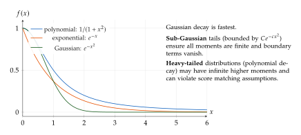
Comparison of polynomial, exponential, and Gaussian decay rates. Schwartz-class functions such as Gaussians decay faster than any polynomial, ensuring that integration-by-parts boundary terms vanish.

The hierarchy $C^{0} \supset C^{1} \supset C^{2} \supset \dots \supset C^{\infty} \supset 𝒮$ provides increasingly strong regularity. For many purposes in generative modelling, $C^{2}$ suffices (since we need second derivatives for the Hessian trace in score matching), but the Schwartz class is the “gold standard” where all analytical manipulations are guaranteed to be valid.

We briefly introduce Sobolev spaces, which provide the natural functional-analytic setting for score functions and weak derivatives. While we will not need the full theory of Sobolev spaces, it is worth understanding the basic idea, as it explains why neural networks with non-smooth activations can still be analysed rigorously.

Definition 41 (Sobolev Space (Informal)).

The Sobolev space $W^{k, p} (Ω)$ consists of functions defined on $Ω \subseteq ℝ^{n}$ whose weak derivatives up to order $k$ all belong to $L^{p} (Ω)$ . The most commonly encountered case in generative modelling is $\begin{matrix} W^{1,2} (Ω) = H^{1} (Ω), \end{matrix}$ the space of functions with square-integrable first derivatives. A function $f \in H^{1}$ may not be classically differentiable everywhere, but possesses a well-defined gradient in the $L^{2}$ sense.

Remark 11 (Why Sobolev Spaces Matter).

Sobolev spaces provide the natural setting for score functions. A score $\nabla_{𝒙} \log p (𝒙)$ that belongs to an appropriate Sobolev space has enough regularity for integration by parts to hold in the weak (distributional) sense, even when classical derivatives may not exist at isolated points. This allows the theory to cover neural network score models that use non-smooth activations like ReLU, provided their outputs have square-integrable gradients almost everywhere.

Understanding which regularity class a function belongs to is important in generative modelling for several reasons. First, score matching requires the model log-density to be at least $C^{2}$ so that the Hessian trace $trace (\nabla^{2} \log p_{θ})$ exists. Second, the convergence theory of diffusion models relies on the score function satisfying Lipschitz conditions, which places the score in $C^{0,1}$ (Lipschitz continuous but not necessarily differentiable). Third, neural networks with smooth activations (such as GELU or softplus) produce $C^{\infty}$ outputs, while those using ReLU produce only $C^{0}$ outputs, with consequences for the regularity of the learned density.

The following assumptions collect the standard regularity conditions used in score matching and related results throughout this text. These are not merely technical requirements: each corresponds to a failure mode that can arise in practice when the assumptions are violated.

Assumption 1 (Score Regularity).

The model score function $𝒔_{θ} (𝒙) = \nabla_{𝒙} \log p_{θ} (𝒙)$ is continuously differentiable in $𝒙$ for each $θ$ , and satisfies the finite Fisher information condition: (Score REG) $\begin{matrix} 𝔼_{p_{d}} [{‖ 𝒔_{θ} (𝒙) ‖}^{2}] < \infty . \end{matrix}$

Assumption 2 (Boundary Decay).

The product of the data density and the model score vanishes at infinity: (Boundary) $\begin{matrix} p_{d} (𝒙) \cdot 𝒔_{θ} (𝒙) \to 0 as ‖ 𝒙 ‖ \to \infty, \end{matrix}$ ensuring that the boundary terms arising from integration by parts are zero.

Assumption 3 (Positivity).

The model density is everywhere positive: $p_{θ} (𝒙) > 0$ for all $𝒙 \in ℝ^{n}$ and all $θ$ in the parameter space. This ensures that the score function $\nabla_{𝒙} \log p_{θ} (𝒙)$ is well-defined everywhere.

Assumption 4 (Identifiability).

The model family ${p_{θ}}$ is identifiable: if $p_{θ_{1}} (𝒙) = p_{θ_{2}} (𝒙)$ for almost every $𝒙$ , then $θ_{1} = θ_{2}$ . This ensures that the minimiser of the score matching objective, if it exists, uniquely determines the model parameters.

These four assumptions together form the standard regularity package for score matching. Assumptions Assumption 1 and Assumption 2 are needed for the integration-by-parts step, Assumption 3 ensures the score is everywhere defined, and Assumption 4 ensures that the optimisation problem has a unique solution. When any of these assumptions is violated, the score matching estimator may be inconsistent, have infinite variance, or converge to the wrong parameter values.

In practice, neural network score models with smooth activations, trained on data from sub-Gaussian distributions, satisfy these assumptions at least approximately. The theoretical analysis assuming exact satisfaction provides guidance for architecture and distribution choices, even when the assumptions hold only in an approximate sense.

Contraction Mappings and Fixed Points

Many iterative algorithms in machine learning can be understood through the lens of contraction mappings. The central question is simple: given a mapping $T$ that we apply repeatedly, does the sequence of iterates $x_{0}, T (x_{0}), T (T (x_{0})), \dots$ converge, and if so, to what? The Banach fixed point theorem provides a clean and complete answer when $T$ is a contraction: the iterates always converge to a unique fixed point, regardless of the starting point, and the convergence rate is geometric. This makes it one of the most practical existence theorems in all of mathematics.

Definition 42 (Contraction Mapping).

Let $(X, d)$ be a metric space. A function $T : X \to X$ is a contraction mapping (or contraction) if there exists a constant $0 \leq κ < 1$ such that (Contraction) $\begin{matrix} d (T (x), T (y)) \leq κ \cdot d (x, y) for all x, y \in X . \end{matrix}$ The constant $κ$ is called the contraction factor. Every contraction is Lipschitz continuous with Lipschitz constant $κ < 1$ , and in particular is uniformly continuous.

Example 21 (A Simple Contraction).

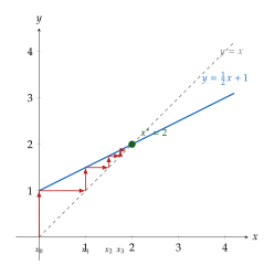
The map $T (x) = \frac{1}{2} x + 1$ on $(ℝ, | \cdot |)$ is a contraction with factor $κ = 1 / 2$ , since $| T (x) - T (y) | = \frac{1}{2} | x - y |$ . Its unique fixed point satisfies $x^{*} = \frac{1}{2} x^{*} + 1$ , giving $x^{*} = 2$ . Starting from $x_{0} = 0$ , the iterates are $x_{n} = 2 (1 - 2^{- n})$ , which converge geometrically to $2$ . This example, despite its simplicity, illustrates the key features of the theorem: existence, uniqueness, and a concrete convergence rate.

Theorem 31 (Banach Fixed Point Theorem).

Let $(X, d)$ be a complete metric space and $T : X \to X$ a contraction with factor $κ \in [0, 1)$ . Then:

$T$ has a unique fixed point $x^{*}$ , i.e., $T (x^{*}) = x^{*}$ .
For any starting point $x_{0} \in X$ , the iterates $x_{n + 1} = T (x_{n})$ converge to $x^{*}$ .
The rate of convergence is geometric: (Banach RATE) $\begin{matrix} d (x_{n}, x^{*}) \leq \frac{κ^{n}}{1 - κ} d (x_{0}, x_{1}) . \end{matrix}$

Proof.

Existence. Fix any $x_{0} \in X$ and define $x_{n} = T (x_{n - 1})$ for $n \geq 1$ . We first show that ${x_{n}}$ is a Cauchy sequence. By the contraction property, $d (x_{n + 1}, x_{n}) = d (T (x_{n}), T (x_{n - 1})) \leq κ d (x_{n}, x_{n - 1}) \leq \dots \leq κ^{n} d (x_{1}, x_{0}) .$ For any $m > n$ , the triangle inequality gives (Cauchy Bound) $\begin{matrix} d (x_{m}, x_{n}) & \leq \sum_{k = n}^{m - 1} d (x_{k + 1}, x_{k}) \leq d (x_{1}, x_{0}) \sum_{k = n}^{m - 1} κ^{k} \leq d (x_{1}, x_{0}) \frac{κ^{n}}{1 - κ} . \end{matrix}$ Since $κ < 1$ , the right-hand side tends to zero as $n \to \infty$ , so ${x_{n}}$ is Cauchy. By completeness of $(X, d)$ , there exists $x^{*} \in X$ with $x_{n} \to x^{*}$ .

$x^{*}$ is a fixed point. We show $T (x^{*}) = x^{*}$ using the triangle inequality: $d (T (x^{*}), x^{*}) \leq d (T (x^{*}), T (x_{n})) + d (x_{n + 1}, x^{*}) \leq κ d (x^{*}, x_{n}) + d (x_{n + 1}, x^{*}) \to 0.$ Hence $d (T (x^{*}), x^{*}) = 0$ , so $T (x^{*}) = x^{*}$ .

Uniqueness. Suppose $T (x^{*}) = x^{*}$ and $T (y^{*}) = y^{*}$ . Then $d (x^{*}, y^{*}) = d (T (x^{*}), T (y^{*})) \leq κ d (x^{*}, y^{*})$ . Since $κ < 1$ , this forces $d (x^{*}, y^{*}) = 0$ , so $x^{*} = y^{*}$ .

Convergence rate. Letting $m \to \infty$ in (Cauchy Bound) gives $d (x^{*}, x_{n}) \leq κ^{n} d (x_{1}, x_{0}) / (1 - κ)$ . This is a geometric (exponential) rate: the error decreases by a factor of at least $κ$ at each iteration.

∎

The beauty of the Banach fixed point theorem lies in its constructive nature: unlike many existence theorems in analysis (such as those relying on Zorn's lemma or the axiom of choice), it not only asserts that a fixed point exists but provides an explicit algorithm (repeated iteration) to find it and a quantitative bound on how quickly the algorithm converges. This constructive character makes it particularly valuable in computational settings, where an existence result is only useful if accompanied by a practical method to compute the object in question.

The error bound in part (iii) is an a priori estimate: it depends only on the starting point $x_{0}$ , the first iterate $x_{1}$ , and the contraction factor $κ$ , not on the (unknown) fixed point $x^{*}$ . This makes it directly computable before the algorithm terminates.

Cobweb diagram for the contraction

T (x) = \frac{1}{2} x + 1

with fixed point

x^{*} = 2

. Starting from

x_{0} = 0

, the iterates

x_{1} = 1

x_{2} = 1.5

x_{3} = 1.75, \dots

converge geometrically to

x^{*}

with contraction factor

κ = 1 / 2

Key Idea.

The Sinkhorn algorithm for optimal transport converges because each Sinkhorn iteration is a contraction mapping on the space of scaling vectors (in the Hilbert projective metric). The Banach fixed point theorem guarantees geometric convergence to the unique optimal coupling. Similarly, many iterative algorithms in machine learning can be analysed as contractions or approximate contractions:

Expectation-maximisation (EM): Under regularity conditions, the EM operator is a contraction near the true parameter value, giving local geometric convergence.
Proximal gradient methods: The proximal operator of a strongly convex function is a contraction, ensuring convergence of iterative proximal algorithms.
Belief propagation on trees: Message-passing updates on tree-structured graphical models are contractions, guaranteeing convergence to the exact marginals.

The contraction factor $κ$ directly controls how many iterations are needed to reach a desired accuracy: to achieve $d (x_{n}, x^{*}) \leq ε$ , we need $n \geq \log (ε (1 - κ) / d (x_{0}, x_{1})) / \log κ$ iterations.

Historical Note.

Stefan Banach proved his fixed point theorem in his 1922 doctoral thesis at the University of Lwów (now Lviv, Ukraine), making it one of the earliest results in the then-nascent field of functional analysis. Despite its remarkably simple proof, the theorem has proved to be one of the most widely applied existence and uniqueness results in all of mathematics. Picard's existence theorem for ordinary differential equations (1890), the convergence of Newton's method near a root, the implicit function theorem, and the uniqueness of solutions to certain integral equations are all consequences or close relatives of Banach's theorem. In the words of the mathematician Jean Dieudonné, it is “one of the most fertile ideas of modern analysis.”

Exercises

The following exercises reinforce the material from all sections of this appendix. They range from routine verifications (suitable for building intuition) to more substantial proofs. Exercises marked with a generative-modelling flavour connect abstract results to the applications developed in the main text.

Exercise 1 (Supremum Characterisation).

Let $S \subseteq ℝ$ be a nonempty set that is bounded above, and let $s = \sup S$ . Prove that for every $ε > 0$ , there exists an element $x \in S$ such that $s - ε < x \leq s$ . State and prove the analogous result for the infimum.

Exercise 2 (Arithmetic of Suprema).

Let $A$ and $B$ be nonempty bounded subsets of $ℝ$ . Define $A + B = {a + b | a \in A, b \in B}$ . Prove that $\sup (A + B) = \sup A + \sup B and \inf (A + B) = \inf A + \inf B .$

Exercise 3 (Epsilon– $N$ Convergence).

Using the $ε$ – $N$ definition of convergence, prove that the sequence $a_{n} = \frac{3 n + 1}{n + 2}$ converges to $3$ as $n \to \infty$ . That is, given $ε > 0$ , find an explicit $N \in ℕ$ such that $| a_{n} - 3 | < ε$ for all $n \geq N$ . Hint: first simplify $| a_{n} - 3 |$ algebraically.

Exercise 4 (Closed Sets and Limit Points).

Let $(X, d)$ be a metric space and let $A \subseteq X$ . Prove that $A$ is closed if and only if $A$ contains all of its limit points.

Exercise 5 (Cauchy Sequences Are Bounded).

Let $(X, d)$ be a metric space and let ${x_{n}}$ be a Cauchy sequence in $X$ . Prove that ${x_{n}}$ is bounded, i.e., there exists $M > 0$ and $x_{0} \in X$ such that $d (x_{n}, x_{0}) \leq M$ for all $n$ . Hint: use the Cauchy property with $ε = 1$ to control all but finitely many terms, then handle the finitely many remaining terms separately.

Exercise 6 (Heine–Borel in $ℝ$ ).

Prove the Heine–Borel theorem for $ℝ$ : a subset $K \subseteq ℝ$ is compact if and only if it is closed and bounded. Hint: for the “if” direction, use the Bolzano–Weierstrass theorem to extract a convergent subsequence from any sequence in $K$ .

Exercise 7 (Continuity vs. Uniform Continuity).

Prove that $f (x) = x^{2}$ is continuous but not uniformly continuous on $ℝ$ . Specifically, show that for any $δ > 0$ , there exist $x, y \in ℝ$ with $| x - y | < δ$ but $| f (x) - f (y) | \geq 1$ . Hint: choose $x$ large enough that the slope of $f$ near $x$ exceeds $1 / δ$ . What does this tell you about why unbounded domains require care in optimisation?

Exercise 8 (Lipschitz Algebra).

Let $f, g : ℝ \to ℝ$ be Lipschitz continuous with Lipschitz constants $L_{f}$ and $L_{g}$ respectively. Prove:

$f + g$ is Lipschitz with constant at most $L_{f} + L_{g}$ .
$f \circ g$ is Lipschitz with constant at most $L_{f} \cdot L_{g}$ .
Give an example showing that $f \cdot g$ need not be Lipschitz, even when both $f$ and $g$ are Lipschitz. Hint: try $f (x) = g (x) = x$ .

Exercise 9 (Gaussian Score Function).

Let $p (x) = \frac{1}{\sqrt{2 π}} e^{- x^{2} / 2}$ be the standard Gaussian density.

Compute the score function $\nabla_{x} \log p (x)$ .
Compute the Hessian $\nabla_{x}^{2} \log p (x)$ .
Verify that $p (x) \cdot \nabla_{x} \log p (x) \to 0$ as $| x | \to \infty$ .
Compute $𝔼_{p} [{‖ \nabla_{x} \log p (x) ‖}^{2}]$ and verify it equals $trace (- \nabla_{x}^{2} \log p (x)) = 1$ (consistent with the score matching identity).

Exercise 10 (Change of Variables for Affine Transforms).

Let $Z \sim 𝒩 (0, 1)$ and define $X = μ + σ Z$ for constants $μ \in ℝ$ and $σ > 0$ . Use the change-of-variables formula (Theorem 26) to show that $X$ has density $p_{X} (x) = \frac{1}{σ \sqrt{2 π}} \exp (- \frac{{(x - μ)}^{2}}{2 σ^{2}}) .$

Exercise 11 (Integration by Parts Computation).

Apply integration by parts to compute $\int_{0}^{\infty} x e^{- x} d x$ without using the gamma function directly. Then generalise: use repeated integration by parts to show that $\int_{0}^{\infty} x^{n} e^{- x} d x = n!$ for all $n \in ℕ$ .

Exercise 12 (Failure of Boundary Decay).

Give an example of a probability density $p \in C^{\infty} (ℝ)$ that does not satisfy the boundary decay condition (Assumption 2) for some reasonable model score $𝒔_{θ}$ . Explain what goes wrong when one attempts to apply integration by parts in the score matching derivation. Hint: consider a density whose tails oscillate, such as a smooth density with bumps at $x = n$ for $n = 1, 2, 3, \dots$ whose heights decrease but whose score values do not decay fast enough.

Exercise 13 (Cauchy Distribution and Score Regularity).

Consider the Cauchy density $p (x) = \frac{1}{π (1 + x^{2})}$ .

Show that $p$ has a well-defined score function $\nabla_{x} \log p (x) = - 2 x / (1 + x^{2})$ .
Prove that $𝔼_{p} [{| \nabla_{x} \log p (x) |}^{2}] = \infty$ , violating the score regularity assumption (Assumption 1).
Explain the practical implications: why does this make score matching unreliable for heavy-tailed data?

Exercise 14 (Cosine Contraction).

Let $T (x) = \cos (x)$ restricted to the interval $[0, π / 2]$ .

Show that $T$ maps $[0, π / 2]$ into itself.
Show that $T$ is a contraction on $[0, π / 2]$ and find an upper bound on the contraction factor. Hint: use the mean value theorem and $| T^{'} (x) | = | \sin (x) | \leq 1$ . Can you find a tighter bound?
Starting from $x_{0} = 1$ , compute 10 iterates $x_{1}, x_{2}, \dots, x_{10}$ and report the fixed point to 4 decimal places.

Exercise 15 (Newton's Method as a Contraction).

For a fixed $a > 0$ , consider the iteration $x_{n + 1} = T (x_{n})$ where $T (x) = \frac{1}{2} (x + a / x)$ (Newton's method for computing $\sqrt{a}$ ).

Show that $T$ maps $[\sqrt{a}, \infty)$ into itself.
Compute $T^{'} (x)$ and show that $| T^{'} (x) | \leq \frac{1}{2}$ for all $x \geq \sqrt{a}$ , so $T$ is a contraction on $[\sqrt{a}, \infty)$ with factor $κ \leq 1 / 2$ .
Identify the unique fixed point of $T$ and explain why the iterates converge to $\sqrt{a}$ .
In practice, Newton's method for square roots converges much faster than the geometric rate $κ = 1 / 2$ suggests. Explain why. Hint: consider the error $e_{n} = x_{n} - \sqrt{a}$ and show that $e_{n + 1} = e_{n}^{2} / (2 x_{n})$ , giving quadratic convergence.

Exercise 16 (Weak but Not Strong Convergence in $ℓ^{2}$ ).

In the Hilbert space $ℓ^{2}$ of square-summable sequences, let $𝒆_{n}$ denote the sequence with $1$ in position $n$ and $0$ elsewhere.

Show that $‖ 𝒆_{n} ‖ = 1$ for all $n$ , so ${𝒆_{n}}$ does not converge strongly to $0$ (or to any other element).
Prove that $𝒆_{n} ⇀ 0$ weakly, meaning $⟨ 𝒆_{n}, 𝒇 ⟩ \to 0$ for every $𝒇 \in ℓ^{2}$ . Hint: for $𝒇 = (f_{1}, f_{2}, \dots) \in ℓ^{2}$ , observe that $⟨ 𝒆_{n}, 𝒇 ⟩ = f_{n}$ and use the fact that $\sum_{n} {| f_{n} |}^{2} < \infty$ implies $f_{n} \to 0$ .
Explain why this example shows that the unit ball in an infinite-dimensional Hilbert space is not sequentially compact in the strong topology, but is sequentially compact in the weak topology (by the Banach–Alaoglu theorem). Why does this distinction matter for convergence of probability measures in generative modelling?

← 42 Distributed Generative AI B Convex Analysis →

A Mathematical Analysis

The Real Number Line

Metric Spaces

Definition and Examples

Open and Closed Sets

Interior, Closure, and Boundary

Sequences and Convergence

Compactness

Continuity

Definitions of Continuity

Extreme Value Theorem

Uniform Continuity

Lipschitz Continuity

Connectedness

Normed and Inner Product Spaces

Normed Vector Spaces

Lp Function Spaces

Inner Product Spaces

Banach and Hilbert Spaces

Topology

Topological Spaces

Strong and Weak Topologies

Differentiation and Integration in ℝn⁡

Gradients, Jacobians, and Hessians

Integration by Parts

Change of Variables

Dominated Convergence Theorem

Leibniz Integral Rule

Regularity and Function Classes

Contraction Mappings and Fixed Points

Exercises

$L^{p}$ Function Spaces

Differentiation and Integration in $ℝ^{n}$