B Convex Analysis

Convexity is one of the most powerful structural assumptions in optimisation. When both the objective and feasible region are convex, local optima are global optima, duality theory provides certificates of optimality, and efficient algorithms exist with provable convergence guarantees. In generative modelling, convex analysis underpins Wasserstein distances (via Kantorovich duality), $f$ -divergences (via Fenchel conjugates), and the ELBO derivation (via Jensen's inequality). This appendix develops the core ideas from first principles, emphasising the results that appear most frequently in the main text.

Convex Sets

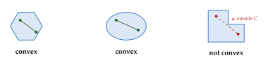
The notion of convexity begins with geometry. A region is convex if, intuitively, you can walk in a straight line between any two of its points without ever leaving the region. This simple geometric property has remarkably deep consequences for analysis and optimisation.

Definition 1 (Convex Set).

A set $C \subseteq ℝ^{n}$ is convex if for every pair of points $𝒙, 𝒚 \in C$ and every scalar $θ \in [0,1]$ , the point $θ 𝒙 + (1 - θ) 𝒚$ also lies in $C$ . In other words, the line segment connecting any two points of $C$ is entirely contained in $C$ .

Familiar examples abound: the real line $ℝ$ , any subspace, any halfspace ${𝒙 : \dot{𝐚} 𝒙 \leq b}$ , and the Euclidean ball ${𝒙 : ‖ 𝒙 ‖ \leq r}$ are all convex. The empty set and singleton sets are convex by convention (the defining condition holds vacuously or trivially).

Definition 2 (Convex Combination).

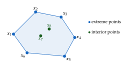
A point $𝒙$ is a convex combination of points $𝒙_{1}, \dots, 𝒙_{k}$ if it can be written as (Combination) $\begin{matrix} 𝒙 = θ_{1} 𝒙_{1} + θ_{2} 𝒙_{2} + \dots + θ_{k} 𝒙_{k}, \end{matrix}$ where $θ_{i} \geq 0$ for all $i$ and $θ_{1} + θ_{2} + \dots + θ_{k} = 1$ .

Convex combinations generalise the two-point definition: a set is convex if and only if it contains all convex combinations of its points. For $k = 2$ , we recover the original definition. For $k = 3$ , convex combinations sweep out a triangle; for general $k$ , they form a simplex.

Definition 3 (Convex Hull).

The convex hull of a set $S \subseteq ℝ^{n}$ , denoted $conv (S)$ , is the set of all convex combinations of points in $S$ : (HULL) $\begin{matrix} conv (S) = {\sum_{i = 1}^{k} θ_{i} 𝒙_{i} | k \in ℕ, 𝒙_{i} \in S, θ_{i} \geq 0, \sum_{i = 1}^{k} θ_{i} = 1} . \end{matrix}$ Equivalently, $conv (S)$ is the smallest convex set containing $S$ : the intersection of all convex sets that contain $S$ .

The equivalence of these two characterisations is instructive. The intersection definition immediately shows that $conv (S)$ is convex (by Theorem 1 below), while the explicit formula makes it computable. In computational geometry, finding the convex hull of a finite point set is a fundamental problem with $O (n \log n)$ algorithms in two dimensions.

Convex vs. non-convex sets. In the convex sets (left, centre), every line segment between interior points remains inside the set. In the L-shaped region (right), the dashed segment between two points of

C

passes through a region outside

C

The convex hull of eight points in

ℝ^{2}

. The extreme points

𝒙_{1}, \dots, 𝒙_{6}

lie on the boundary of

conv {𝒙_{1}, \dots, 𝒙_{8}}

, while

𝒙_{7}

and

𝒙_{8}

lie in the interior and can be expressed as convex combinations of the extreme points.

Definition 4 (Affine Function).

A function $f : ℝ^{n} \to ℝ^{m}$ is affine if $f (𝒙) = A 𝒙 + 𝐛$ for some matrix $A \in ℝ^{m \times n}$ and vector $𝐛 \in ℝ^{m}$ . An affine function is simultaneously convex and concave.

Theorem 1 (Operations Preserving Convexity).

The following operations preserve convexity of sets:

Intersection. If ${C_{α}}_{α \in 𝒜}$ is any (possibly infinite) family of convex sets, then $⋂_{α \in 𝒜} C_{α}$ is convex.
Affine image. If $C$ is convex and $f (𝒙) = A 𝒙 + 𝐛$ is affine, then $f (C) = {A 𝒙 + 𝐛 : 𝒙 \in C}$ is convex.
Minkowski sum. If $A$ and $B$ are convex, then $A + B = {𝐚 + 𝐛 : 𝐚 \in A, 𝐛 \in B}$ is convex.

Proof.

Part (i). Let $𝒙, 𝒚 \in ⋂_{α} C_{α}$ and $θ \in [0,1]$ . For each $α$ , both $𝒙$ and $𝒚$ belong to $C_{α}$ , and since $C_{α}$ is convex, $θ 𝒙 + (1 - θ) 𝒚 \in C_{α}$ . Since this holds for every $α$ , we have $θ 𝒙 + (1 - θ) 𝒚 \in ⋂_{α} C_{α}$ .

Part (ii). Let $𝐮, 𝐯 \in f (C)$ , so $𝐮 = A 𝒙 + 𝐛$ and $𝐯 = A 𝒚 + 𝐛$ for some $𝒙, 𝒚 \in C$ . Then $θ 𝐮 + (1 - θ) 𝐯 = A (θ 𝒙 + (1 - θ) 𝒚) + 𝐛 .$ Since $C$ is convex, $θ 𝒙 + (1 - θ) 𝒚 \in C$ , so the right-hand side belongs to $f (C)$ .

Part (iii). Let $𝐮_{1} = 𝐚_{1} + 𝐛_{1}$ and $𝐮_{2} = 𝐚_{2} + 𝐛_{2}$ with $𝐚_{i} \in A$ , $𝐛_{i} \in B$ . For $θ \in [0,1]$ : $θ 𝐮_{1} + (1 - θ) 𝐮_{2} = \underset{\in A}{\underset{⏟}{(θ 𝐚_{1} + (1 - θ) 𝐚_{2})}} + \underset{\in B}{\underset{⏟}{(θ 𝐛_{1} + (1 - θ) 𝐛_{2})}},$ where the two terms lie in $A$ and $B$ respectively by convexity. Hence the sum belongs to $A + B$ .

∎

Key Idea.

In machine learning, many constraint sets are convex: the probability simplex $Δ^{k - 1} = {𝒙 \in ℝ^{k} : x_{i} \geq 0, \sum_{i} x_{i} = 1}$ (probability vectors), the unit ball ${𝒙 : ‖ 𝒙 ‖ \leq 1}$ (weight decay), the cone of positive semidefinite matrices $𝕊_{+}^{n}$ (kernel methods), and the Birkhoff polytope of doubly stochastic matrices (optimal transport). Even when the objective is non-convex (as in training neural networks), recognising convex constraint structure enables powerful algorithmic tools such as projected gradient descent and Frank–Wolfe methods.

Convex Functions

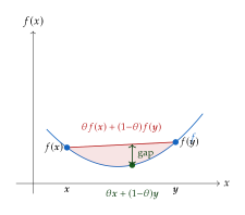
Having established the geometry of convex sets, we turn to convex functions, which are the analytic counterpart. The graph of a convex function curves upward (or is flat), so that any secant line lies above the curve. This simple shape constraint leads to a rich theory of inequalities, optimality conditions, and duality.

Definition 5 (Convex Function).

A function $f : ℝ^{n} \to ℝ \cup {+ \infty}$ is convex if its effective domain $dom (f) = {𝒙 : f (𝒙) < + \infty}$ is a convex set and, for all $𝒙, 𝒚 \in dom (f)$ and all $θ \in [0,1]$ , (Function DEF) $\begin{matrix} f (θ 𝒙 + (1 - θ) 𝒚) \leq θ f (𝒙) + (1 - θ) f (𝒚) . \end{matrix}$ A function $f$ is concave if $- f$ is convex.

The convention of allowing $f$ to take the value $+ \infty$ is a convenient device: it lets us encode constraints into the objective by setting $f (𝒙) = + \infty$ for infeasible points, unifying constrained and unconstrained optimisation.

Definition 6 (Strictly Convex).

A function $f$ is strictly convex if the inequality in (Function DEF) is strict whenever $𝒙 \neq 𝒚$ and $θ \in (0,1)$ . Geometrically, the chord between any two distinct points on the graph lies strictly above the graph (except at the endpoints).

Definition 7 (Strongly Convex).

A function $f$ is $μ$ -strongly convex (with parameter $μ > 0$ ) if $f (𝒙) - \frac{μ}{2} {‖ 𝒙 ‖}^{2}$ is convex. Equivalently, for all $𝒙, 𝒚 \in dom (f)$ , (Strong) $\begin{matrix} f (𝒚) \geq f (𝒙) + \nabla f {(𝒙)}^{⊤} (𝒚 - 𝒙) + \frac{μ}{2} {‖ 𝒚 - 𝒙 ‖}^{2} . \end{matrix}$ Strong convexity means the function grows at least quadratically away from any tangent hyperplane.

Strong convexity is strictly stronger than strict convexity, which is strictly stronger than convexity. The function $f (x) = x^{4}$ is strictly convex but not strongly convex (its curvature vanishes at the origin). In optimisation, strong convexity is the “gold standard” because it guarantees both uniqueness of the minimiser and linear convergence rates for gradient descent.

Proposition 1 (Unique Minimiser).

If $f : ℝ^{n} \to ℝ \cup {+ \infty}$ is $μ$ -strongly convex with $μ > 0$ , then $f$ has at most one minimiser.

Proof.

Suppose $𝒙^{*}$ and $𝒚^{*}$ are both global minimisers, so $f (𝒙^{*}) = f (𝒚^{*}) = f^{*}$ . Applying the strong convexity condition (Strong) with $𝒙 = 𝒙^{*}$ and $𝒚 = 𝒚^{*}$ : $f (𝒚^{*}) \geq f (𝒙^{*}) + \nabla f {(𝒙^{*})}^{⊤} (𝒚^{*} - 𝒙^{*}) + \frac{μ}{2} {‖ 𝒚^{*} - 𝒙^{*} ‖}^{2} .$ Since $𝒙^{*}$ is a minimiser, the first-order optimality condition gives $\nabla f {(𝒙^{*})}^{⊤} (𝒚^{*} - 𝒙^{*}) \geq 0$ (or, if $f$ is unconstrained, $\nabla f (𝒙^{*}) = 𝟎$ ). Either way, $f^{*} \geq f^{*} + \frac{μ}{2} {‖ 𝒚^{*} - 𝒙^{*} ‖}^{2}$ , which forces ${‖ 𝒚^{*} - 𝒙^{*} ‖}^{2} \leq 0$ , hence $𝒙^{*} = 𝒚^{*}$ .

∎

Jensen's inequality visualised. For a convex function

f

, the value at a convex combination

θ 𝒙 + (1 - θ) 𝒚

lies below the secant line connecting

(x, f (𝒙))

and

(𝒚, f (𝒚))

. The shaded region represents the “Jensen gap.”

Theorem 2 (Jensen's Inequality).

Let $f$ be a convex function and let $X$ be a random variable taking values in $dom (f)$ with $𝔼 [X] \in dom (f)$ . Then (Jensen) $\begin{matrix} f (𝔼 [X]) \leq 𝔼 [f (X)] . \end{matrix}$ If $f$ is concave, the inequality reverses: $f (𝔼 [X]) \geq 𝔼 [f (X)]$ .

Proof.

We proceed by induction on the number of mass points, then extend by a limiting argument.

Base case ( $k = 2$ ). If $X$ takes values $𝒙_{1}, 𝒙_{2}$ with probabilities $θ, 1 - θ$ , then $𝔼 [X] = θ 𝒙_{1} + (1 - θ) 𝒙_{2}$ and $𝔼 [f (X)] = θ f (𝒙_{1}) + (1 - θ) f (𝒙_{2})$ . The inequality $f (𝔼 [X]) \leq 𝔼 [f (X)]$ is precisely the definition of convexity.

Inductive step. Suppose the result holds for $k - 1$ points. Let $X$ take values $𝒙_{1}, \dots, 𝒙_{k}$ with probabilities $θ_{1}, \dots, θ_{k}$ . Without loss of generality, $θ_{1} < 1$ (otherwise the result is trivial). Write $𝔼 [X] = θ_{1} 𝒙_{1} + (1 - θ_{1}) \underset{= \overline{𝒙}}{\underset{⏟}{\sum_{i = 2}^{k} \frac{θ_{i}}{1 - θ_{1}} 𝒙_{i}}} .$ By convexity of $f$ , $f (𝔼 [X]) \leq θ_{1} f (𝒙_{1}) + (1 - θ_{1}) f (\overline{𝒙}) .$ The point $\overline{𝒙}$ is the expectation of a random variable supported on $k - 1$ points with probabilities $θ_{i} / (1 - θ_{1})$ . By the inductive hypothesis, $f (\overline{𝒙}) \leq \sum_{i = 2}^{k} \frac{θ_{i}}{1 - θ_{1}} f (𝒙_{i})$ . Substituting: $f (𝔼 [X]) \leq θ_{1} f (𝒙_{1}) + (1 - θ_{1}) \sum_{i = 2}^{k} \frac{θ_{i}}{1 - θ_{1}} f (𝒙_{i}) = \sum_{i = 1}^{k} θ_{i} f (𝒙_{i}) = 𝔼 [f (X)] .$

Extension to continuous distributions. For a general random variable $X$ with density, approximate $X$ by discrete random variables $X_{n}$ (e.g., by quantisation) and pass to the limit using the dominated convergence theorem and lower semicontinuity of $f$ .

∎

Historical Note.

Jensen's inequality is named after Johan Jensen, who published it in 1906, although the result for finite sums was known earlier. Jensen was a Danish mathematician and engineer who worked for the Copenhagen Telephone Company. His inequality has become one of the most widely used tools in probability, information theory, and statistical physics.

Key Idea.

Jensen's inequality is arguably the single most important inequality in variational inference. The entire evidence lower bound (ELBO) rests on applying Jensen to the concave logarithm: $\log 𝔼_{q} [\frac{p (𝒙, 𝒛)}{q (𝒛)}] \geq 𝔼_{q} [\log \frac{p (𝒙, 𝒛)}{q (𝒛)}] .$ Every VAE, every diffusion model's variational bound, and every EM algorithm traces back to this one application of convexity. Understanding when the inequality is tight (when $p (𝒙, 𝒛) / q (𝒛)$ is almost surely constant, i.e., when $q$ closely matches the true posterior) guides the design of better approximate posteriors.

Theorem 3 (First-Order Condition).

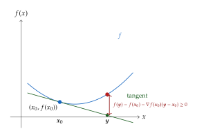
Let $f : ℝ^{n} \to ℝ$ be differentiable on an open convex domain. Then $f$ is convex if and only if for all $𝒙, 𝒚 \in dom (f)$ , (First Order) $\begin{matrix} f (𝒚) \geq f (𝒙) + \nabla f {(𝒙)}^{⊤} (𝒚 - 𝒙) . \end{matrix}$ Geometrically, the tangent hyperplane at any point is a global underestimator of the function.

Proof.

( $⟹$ ) Assume $f$ is convex. For any $θ \in (0, 1]$ , convexity gives $f (𝒙 + θ (𝒚 - 𝒙)) \leq (1 - θ) f (𝒙) + θ f (𝒚),$ which we rearrange to $f (𝒚) \geq f (𝒙) + \frac{f (𝒙 + θ (𝒚 - 𝒙)) - f (𝒙)}{θ} .$ Taking $θ \to 0^{+}$ , the right-hand side converges to $f (𝒙) + \nabla f {(𝒙)}^{⊤} (𝒚 - 𝒙)$ by the definition of the gradient.

( $⟸$ ) Assume (First Order) holds. Fix $𝒙, 𝒚 \in dom (f)$ and $θ \in [0,1]$ , and let $𝒛 = θ 𝒙 + (1 - θ) 𝒚$ . Apply the first-order condition at $𝒛$ in two directions: $\begin{matrix} f (𝒙) & \geq f (𝒛) + \nabla f {(𝒛)}^{⊤} (𝒙 - 𝒛), \\ f (𝒚) & \geq f (𝒛) + \nabla f {(𝒛)}^{⊤} (𝒚 - 𝒛) . \end{matrix}$ Multiply the first inequality by $θ$ and the second by $1 - θ$ , then add: $θ f (𝒙) + (1 - θ) f (𝒚) \geq f (𝒛) + \nabla f (𝒛)^{⊤} (θ (𝒙 - 𝒛) + (1 - θ) (𝒚 - 𝒛)) .$ The second term vanishes because $θ (𝒙 - 𝒛) + (1 - θ) (𝒚 - 𝒛) = θ 𝒙 + (1 - θ) 𝒚 - 𝒛 = 𝟎$ . Therefore $θ f (𝒙) + (1 - θ) f (𝒚) \geq f (𝒛)$ , which is precisely convexity.

∎

The first-order condition for convexity. The tangent line (or hyperplane) at any point

𝒙_{0}

lies entirely below the graph of a convex function

f

. The vertical gap

f (𝒚) - [f (𝒙_{0}) + \nabla f {(𝒙_{0})}^{⊤} (𝒚 - 𝒙_{0})]

is non-negative for all

𝒚

Theorem 4 (Second-Order Condition).

Let $f : ℝ^{n} \to ℝ$ be twice continuously differentiable on an open convex domain. Then:

$f$ is convex if and only if the Hessian is positive semidefinite everywhere: $\nabla^{2} f (𝒙) ⪰ 0$ for all $𝒙 \in dom (f)$ .
$f$ is $μ$ -strongly convex if and only if $\nabla^{2} f (𝒙) ⪰ μ I$ for all $𝒙 \in dom (f)$ .

Proof.

We prove part (i); part (ii) follows by applying (i) to $g (𝒙) = f (𝒙) - \frac{μ}{2} {‖ 𝒙 ‖}^{2}$ .

( $⟹$ ) Suppose $f$ is convex. Fix $𝒙$ and any direction $𝐯 \in ℝ^{n}$ . The univariate function $g (t) = f (𝒙 + t 𝐯)$ is convex in $t$ (as the composition of $f$ with an affine map). A convex function of one variable has non-negative second derivative wherever it exists, so $g^{''} (0) = 𝐯^{⊤} \nabla^{2} f (𝒙) 𝐯 \geq 0.$ Since $𝐯$ is arbitrary, $\nabla^{2} f (𝒙) ⪰ 0$ .

( $⟸$ ) Suppose $\nabla^{2} f (𝒙) ⪰ 0$ for all $𝒙$ . By Taylor's theorem with integral remainder, for any $𝒙, 𝒚$ : $f (𝒚) = f (𝒙) + \nabla f {(𝒙)}^{⊤} (𝒚 - 𝒙) + \frac{1}{2} {(𝒚 - 𝒙)}^{⊤} \nabla^{2} f (𝒛) (𝒚 - 𝒙)$ for some $𝒛$ on the line segment between $𝒙$ and $𝒚$ . Since $\nabla^{2} f (𝒛) ⪰ 0$ , the last term is non-negative, giving $f (𝒚) \geq f (𝒙) + \nabla f {(𝒙)}^{⊤} (𝒚 - 𝒙)$ , which is the first-order condition for convexity.

∎

Theorem 5 (Operations Preserving Convexity of Functions).

The following operations preserve convexity of functions:

Non-negative weighted sum. If $f_{1}, \dots, f_{m}$ are convex and $α_{1}, \dots, α_{m} \geq 0$ , then $\sum_{i = 1}^{m} α_{i} f_{i}$ is convex.
Pointwise maximum. If ${f_{i}}_{i \in ℐ}$ is any family of convex functions, then $g (𝒙) = \sup_{i \in ℐ} f_{i} (𝒙)$ is convex.
Composition with affine mapping. If $f$ is convex, then $g (𝒙) = f (A 𝒙 + 𝐛)$ is convex for any matrix $A$ and vector $𝐛$ .

Proof.

Part (i). For $θ \in [0,1]$ : $\begin{matrix} \sum_{i} α_{i} f_{i} (θ 𝒙 + (1 - θ) 𝒚) & \leq \sum_{i} α_{i} [θ f_{i} (𝒙) + (1 - θ) f_{i} (𝒚)] \\ = θ \sum_{i} α_{i} f_{i} (𝒙) + (1 - θ) \sum_{i} α_{i} f_{i} (𝒚), \end{matrix}$ where the inequality uses convexity of each $f_{i}$ and non-negativity of each $α_{i}$ .

Part (ii). For $θ \in [0,1]$ and each $i$ : $f_{i} (θ 𝒙 + (1 - θ) 𝒚) \leq θ f_{i} (𝒙) + (1 - θ) f_{i} (𝒚) \leq θ g (𝒙) + (1 - θ) g (𝒚) .$ Taking the supremum over $i$ on the left gives $g (θ 𝒙 + (1 - θ) 𝒚) \leq θ g (𝒙) + (1 - θ) g (𝒚)$ .

Part (iii) follows directly from the definition, since the composition $𝒙 \mapsto A 𝒙 + 𝐛$ is affine and preserves convex combinations.

∎

Example 1 (Important Convex Functions).

The following functions arise frequently in machine learning and generative modelling:

Quadratic: $f (x) = x^{2}$ (and more generally $f (𝒙) = 𝒙^{⊤} A 𝒙$ for $A ⪰ 0$ ).
Exponential: $f (x) = e^{x}$ (convex on $ℝ$ ; used in log-sum-exp).
Negative logarithm: $f (x) = - \log x$ on $ℝ_{+ +}$ (the key function behind the ELBO).
Norms: $f (𝒙) = {‖ 𝒙 ‖}_{p}$ for $p \geq 1$ , including the $ℓ_{1}$ -norm (sparsity) and $ℓ_{2}$ -norm (weight decay).
Max: $f (𝒙) = \max (x_{1}, \dots, x_{n})$ (convex as a pointwise maximum of linear functions).
Log-sum-exp: $f (𝒙) = \log (\sum_{i = 1}^{n} e^{x_{i}})$ (the smooth approximation to $\max$ ; convex by Theorem 5(ii) and a limiting argument).

Subgradients

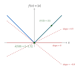
Not all convex functions are differentiable. Consider $f (x) = | x |$ at the origin, or $f (x) = \max (0, x)$ , the ReLU activation that has become ubiquitous in deep learning. At the “kink” of these functions, no single tangent line exists. Yet the geometry of convexity still provides useful linear underestimators. The theory of subgradients extends calculus to non-smooth convex functions, providing the foundation for optimisation algorithms that handle non-differentiable objectives.

Definition 8 (Subgradient).

A vector $𝐠 \in ℝ^{n}$ is a subgradient of a convex function $f$ at a point $𝒙 \in dom (f)$ if (Subgradient) $\begin{matrix} f (𝒚) \geq f (𝒙) + 𝐠^{⊤} (𝒚 - 𝒙) for all 𝒚 \in dom (f) . \end{matrix}$ Geometrically, $𝐠$ defines a supporting hyperplane to the epigraph of $f$ at the point $(𝒙, f (𝒙))$ : the affine function $𝒚 \mapsto f (𝒙) + 𝐠^{⊤} (𝒚 - 𝒙)$ is a global underestimator of $f$ .

Comparing with Theorem 3, we see that at a differentiable point, the gradient $\nabla f (𝒙)$ is the unique subgradient. At non-differentiable points, there may be many subgradients, each defining a different supporting hyperplane.

Definition 9 (Subdifferential).

The subdifferential of $f$ at $𝒙$ , denoted $\partial f (𝒙)$ , is the set of all subgradients of $f$ at $𝒙$ : (Subdifferential) $\begin{matrix} \partial f (𝒙) = {𝐠 \in ℝ^{n} : f (𝒚) \geq f (𝒙) + 𝐠^{⊤} (𝒚 - 𝒙) for all 𝒚} . \end{matrix}$ When $f$ is differentiable at $𝒙$ , the subdifferential reduces to a singleton: $\partial f (𝒙) = {\nabla f (𝒙)}$ .

Subgradients of

f (x) = | x |

. At the kink

x = 0

, any line with slope in

[- 1, 1]

lies below the graph, so

\partial f (0) = [- 1, 1]

(three such lines are shown in red). At the smooth point

x = 2

, the unique tangent line has slope

+ 1

, giving

\partial f (2) = {1}

Theorem 6 (Existence of Subgradients).

Let $f : ℝ^{n} \to ℝ \cup {+ \infty}$ be convex. Then at every point $𝒙$ in the interior of $dom (f)$ , the subdifferential $\partial f (𝒙)$ is nonempty, closed, convex, and compact.

The proof relies on the supporting hyperplane theorem (a consequence of the Hahn–Banach theorem in functional analysis) and is omitted here. The key practical message is that convex functions always admit subgradients at interior points, which guarantees that subgradient-based optimisation methods are always well-defined.

Example 2 (Subdifferentials of Common Functions).

Absolute value, $f (x) = | x |$ : $\partial f (x) = {\begin{matrix} {- 1} & if x < 0, \\ [- 1, 1] & if x = 0, \\ {+ 1} & if x > 0. \end{matrix}$
ReLU, $f (x) = \max (0, x)$ : $\partial f (x) = {\begin{matrix} {0} & if x < 0, \\ [0, 1] & if x = 0, \\ {1} & if x > 0. \end{matrix}$
Pointwise maximum, $f (𝒙) = \max (f_{1} (𝒙), \dots, f_{k} (𝒙))$ where each $f_{i}$ is convex and differentiable: $\partial f (𝒙) = conv {\nabla f_{i} (𝒙) : f_{i} (𝒙) = f (𝒙)},$ the convex hull of the gradients of the “active” functions (those achieving the maximum).

Theorem 7 (Subgradient Optimality Condition).

Let $f : ℝ^{n} \to ℝ \cup {+ \infty}$ be convex. A point $𝒙^{*}$ is a global minimiser of $f$ if and only if $𝟎 \in \partial f (𝒙^{*})$ .

Proof.

( $⟹$ ) Suppose $𝒙^{*}$ minimises $f$ , so $f (𝒚) \geq f (𝒙^{*})$ for all $𝒚$ . This can be rewritten as $f (𝒚) \geq f (𝒙^{*}) + 𝟎^{⊤} (𝒚 - 𝒙^{*})$ , which shows that $𝟎$ is a subgradient of $f$ at $𝒙^{*}$ .

( $⟸$ ) Suppose $𝟎 \in \partial f (𝒙^{*})$ . By definition of the subgradient, $f (𝒚) \geq f (𝒙^{*}) + 𝟎^{⊤} (𝒚 - 𝒙^{*}) = f (𝒙^{*})$ for all $𝒚$ , so $𝒙^{*}$ is a global minimiser.

∎

Remark 1 (Elegance of the Subgradient Condition).

The subgradient optimality condition is striking in its simplicity: checking global optimality of a convex function reduces to checking membership of the zero vector in a set. For smooth functions, this recovers the familiar $\nabla f (𝒙^{*}) = 𝟎$ ; for non-smooth functions, it provides a complete characterisation that no gradient-based condition can.

Key Idea.

Subgradients explain why non-smooth activations like ReLU work in deep learning. Although the gradient of $\max (0, x)$ is undefined at $x = 0$ , the subdifferential $[0, 1]$ provides valid descent directions. In practice, automatic differentiation libraries choose an arbitrary element of the subdifferential (typically $0$ ) at the non-differentiable point, and this works well because the set of inputs that land exactly at a kink has Lebesgue measure zero during training. The theory of Clarke subdifferentials extends these ideas to non-convex functions, providing the theoretical foundation for training deep networks with ReLU, leaky ReLU, and other piecewise-linear activations.

Epigraphs and Sublevel Sets

The epigraph provides a bridge between convex functions and convex sets, allowing us to translate questions about function convexity into questions about set convexity. This perspective is both theoretically elegant and practically powerful: operations that are natural for sets (intersection, projection) correspond to useful operations on functions (pointwise maximum, infimal convolution).

Definition 10 (Epigraph).

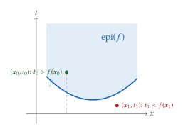
The epigraph of a function $f : ℝ^{n} \to ℝ \cup {+ \infty}$ is the subset of $ℝ^{n + 1}$ defined by (Epigraph) $\begin{matrix} epi (f) = {(𝒙, t) \in ℝ^{n + 1} : f (𝒙) \leq t} . \end{matrix}$ In words, $epi (f)$ is the region “on and above” the graph of $f$ . The name comes from the Greek epi (above).

The epigraph of a convex function

f

. The shaded region above (and including) the graph of

f

epi (f)

. The point

(𝒙_{0}, t_{0})

with

t_{0} > f (𝒙_{0})

lies inside the epigraph, while

(𝒙_{1}, t_{1})

with

t_{1} < f (𝒙_{1})

lies outside.

Theorem 8 (Epigraph Characterisation of Convexity).

A function $f : ℝ^{n} \to ℝ \cup {+ \infty}$ is convex if and only if $epi (f)$ is a convex subset of $ℝ^{n + 1}$ .

Proof.

( $⟹$ ) Suppose $f$ is convex. Let $(𝒙_{1}, t_{1}), (𝒙_{2}, t_{2}) \in epi (f)$ , so $f (𝒙_{1}) \leq t_{1}$ and $f (𝒙_{2}) \leq t_{2}$ . For $θ \in [0,1]$ : $f (θ 𝒙_{1} + (1 - θ) 𝒙_{2}) \leq θ f (𝒙_{1}) + (1 - θ) f (𝒙_{2}) \leq θ t_{1} + (1 - θ) t_{2},$ where the first inequality uses convexity of $f$ and the second uses $f (𝒙_{i}) \leq t_{i}$ . Hence $(θ 𝒙_{1} + (1 - θ) 𝒙_{2}, θ t_{1} + (1 - θ) t_{2}) \in epi (f)$ , proving that $epi (f)$ is convex.

( $⟸$ ) Suppose $epi (f)$ is convex. For any $𝒙_{1}, 𝒙_{2} \in dom (f)$ , the points $(𝒙_{1}, f (𝒙_{1}))$ and $(𝒙_{2}, f (𝒙_{2}))$ lie in $epi (f)$ . By convexity of $epi (f)$ , for $θ \in [0,1]$ : $(θ 𝒙_{1} + (1 - θ) 𝒙_{2}, θ f (𝒙_{1}) + (1 - θ) f (𝒙_{2})) \in epi (f) .$ By the definition of the epigraph, this means $f (θ 𝒙_{1} + (1 - θ) 𝒙_{2}) \leq θ f (𝒙_{1}) + (1 - θ) f (𝒙_{2})$ , which is convexity of $f$ .

∎

The epigraph characterisation is more than a theoretical curiosity. It allows us to prove convexity of complicated functions by showing that their epigraphs can be expressed as intersections of halfspaces (which are convex sets by Theorem 1). This technique is particularly useful for functions defined implicitly as optima of parameterised families.

Definition 11 (Sublevel Set).

For a function $f : ℝ^{n} \to ℝ \cup {+ \infty}$ and a scalar $α \in ℝ$ , the $α$ -sublevel set of $f$ is (Sublevel) $\begin{matrix} S_{α} = {𝒙 \in dom (f) : f (𝒙) \leq α} . \end{matrix}$

Sublevel sets are the horizontal “slices” of the epigraph. For the function $f (𝒙) = {‖ 𝒙 ‖}^{2}$ , the sublevel sets are Euclidean balls ${𝒙 : {‖ 𝒙 ‖}^{2} \leq α}$ . For $f (𝒙) = \max_{i} | x_{i} |$ , they are $ℓ_{\infty}$ -balls.

Theorem 9 (Sublevel Sets of Convex Functions).

If $f : ℝ^{n} \to ℝ \cup {+ \infty}$ is convex, then every sublevel set $S_{α}$ is convex. The converse is false: a function can have all sublevel sets convex without being convex.

Proof.

Suppose $f$ is convex and let $𝒙, 𝒚 \in S_{α}$ , so $f (𝒙) \leq α$ and $f (𝒚) \leq α$ . For $θ \in [0,1]$ : $f (θ 𝒙 + (1 - θ) 𝒚) \leq θ f (𝒙) + (1 - θ) f (𝒚) \leq θ α + (1 - θ) α = α .$ Hence $θ 𝒙 + (1 - θ) 𝒚 \in S_{α}$ , proving $S_{α}$ is convex.

∎

Remark 2 (Converse Fails).

Consider the function $f (x) = - e^{- x^{2}}$ on $ℝ$ . Each sublevel set $S_{α} = {x : - e^{- x^{2}} \leq α}$ is either empty (if $α < - 1$ ), all of $ℝ$ (if $α \geq 0$ ), or a symmetric interval $[- c, c]$ for some $c > 0$ (if $- 1 \leq α < 0$ ). In every case, the sublevel set is convex (an interval). However, $f$ is not convex: it has a local maximum at $x = 0$ and is concave near the origin. Functions whose sublevel sets are all convex are called quasiconvex. Quasiconvexity is a strictly weaker condition than convexity, though it still permits useful optimisation theory; in particular, quasiconvex functions on compact convex sets attain their maxima at extreme points, a fact used in some game-theoretic formulations of generative adversarial networks.

Conjugate Functions and Fenchel Duality

The Fenchel conjugate (also called the convex conjugate or the Legendre–Fenchel transform) is one of the most elegant constructions in convex analysis. It provides a systematic way to convert between primal and dual representations of convex functions, and it is the mathematical engine behind variational representations of divergences in generative modelling. In the next few pages we develop the theory from its definition through the biconjugate theorem and into the concrete conjugate computations that arise in the f-GAN framework.

Definition 12 (Convex Conjugate).

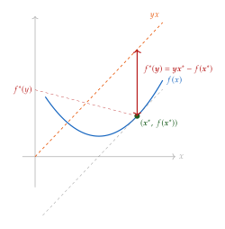
Let $f : ℝ^{n} \to ℝ \cup {+ \infty}$ . The Fenchel conjugate (or convex conjugate) of $f$ is the function $f^{*} : ℝ^{n} \to ℝ \cup {+ \infty}$ defined by (Conjugate DEF) $\begin{matrix} f^{*} (𝒚) = \sup_{𝒙 \in dom f} {𝒚^{⊤} 𝒙 - f (𝒙)} . \end{matrix}$ The domain of $f^{*}$ consists of those $𝒚$ for which the supremum is finite.

Geometrically, $f^{*} (𝒚)$ measures the largest vertical gap between the linear function $𝒙 \mapsto 𝒚^{⊤} 𝒙$ and the graph of $f$ . When $f$ is smooth and strictly convex, the supremum is attained at the unique point $𝒙^{*}$ where $\nabla f (𝒙^{*}) = 𝒚$ , and the conjugate equals $f^{*} (𝒚) = 𝒚^{⊤} 𝒙^{*} - f (𝒙^{*})$ , the $y$ -intercept of the tangent line with slope $𝒚$ . fig:convex:conjugate-geom illustrates this construction.

Geometric interpretation of the Fenchel conjugate. For a given slope

𝒚

(dashed orange line

x \mapsto y x

), the conjugate

f^{*} (𝒚)

is the maximum vertical gap (red) between the line and the convex function

f

(blue). The gap is attained at

𝒙^{*}

where the tangent to

f

has slope

𝒚

Theorem 10 (Conjugate is Always Convex).

For any function $f : ℝ^{n} \to ℝ \cup {+ \infty}$ (not necessarily convex), the conjugate $f^{*}$ is convex and closed (lower semicontinuous).

Proof.

For each fixed $𝒙$ , the map $𝒚 \mapsto 𝒚^{⊤} 𝒙 - f (𝒙)$ is an affine function of $𝒚$ . The conjugate $f^{*} (𝒚) = \sup_{𝒙} {𝒚^{⊤} 𝒙 - f (𝒙)}$ is a pointwise supremum of this family of affine functions. A supremum of convex (in particular, affine) functions is convex (the epigraph of the supremum is the intersection of the individual epigraphs, which are half-spaces, hence convex). Furthermore, each $𝒚 \mapsto 𝒚^{⊤} 𝒙 - f (𝒙)$ is continuous and therefore closed; the supremum of closed functions is closed.

∎

Theorem 11 (Fenchel's Inequality).

For any function $f$ and all $𝒙, 𝒚 \in ℝ^{n}$ , (Fenchel INEQ) $\begin{matrix} f (𝒙) + f^{*} (𝒚) \geq 𝒚^{⊤} 𝒙 . \end{matrix}$

Proof.

By definition, $f^{*} (𝒚) = \sup_{𝒛} {𝒚^{⊤} 𝒛 - f (𝒛)} \geq 𝒚^{⊤} 𝒙 - f (𝒙)$ . Rearranging gives $f (𝒙) + f^{*} (𝒚) \geq 𝒚^{⊤} 𝒙$ .

∎

Theorem 12 (Fenchel–Moreau Biconjugate Theorem).

If $f : ℝ^{n} \to ℝ \cup {+ \infty}$ is closed (lower semicontinuous) and convex, then $f^{* *} = f$ . That is, the conjugate of the conjugate recovers the original function.

Proof.

We show both directions.

( $f^{* *} \leq f$ ). By Theorem 11 applied with $f^{*}$ in place of $f$ , for every $𝒙, 𝒚$ we have $f^{*} (𝒚) + f^{* *} (𝒙) \geq 𝒚^{⊤} 𝒙$ , hence $f^{* *} (𝒙) \geq 𝒚^{⊤} 𝒙 - f^{*} (𝒚)$ for all $𝒚$ . Taking the supremum over $𝒚$ gives $f^{* *} (𝒙) \geq f^{* *} (𝒙)$ , but more directly, applying the original Fenchel inequality to $f$ gives $f^{*} (𝒚) \geq 𝒚^{⊤} 𝒙 - f (𝒙)$ , so $f (𝒙) \geq 𝒚^{⊤} 𝒙 - f^{*} (𝒚)$ for every $𝒚$ . Since $f^{* *} (𝒙) = \sup_{𝒚} {𝒚^{⊤} 𝒙 - f^{*} (𝒚)}$ , we obtain $f^{* *} (𝒙) \leq f (𝒙)$ .

( $f^{* *} \geq f$ ). Because $f$ is closed and convex, it is the pointwise supremum of all affine functions that it dominates: for every $𝒙$ , $f (𝒙) = \sup {a^{⊤} 𝒙 + b : a^{⊤} 𝒛 + b \leq f (𝒛) \forall 𝒛}$ . Each such affine minorant $𝒛 \mapsto a^{⊤} 𝒛 + b$ satisfies $b \leq f (𝒛) - a^{⊤} 𝒛$ for all $𝒛$ , hence $b \leq - f^{*} (a)$ . Therefore $a^{⊤} 𝒙 + b \leq a^{⊤} 𝒙 - f^{*} (a) \leq f^{* *} (𝒙)$ . Taking the supremum over all such $(a, b)$ yields $f (𝒙) \leq f^{* *} (𝒙)$ .

∎

Theorem 13 (Fenchel–Young Equality).

Let $f : ℝ^{n} \to ℝ \cup {+ \infty}$ be a closed convex function. Then (Fenchel Young) $\begin{matrix} f (𝒙) + f^{*} (𝒚) = 𝒚^{⊤} 𝒙 ⟺ 𝒚 \in \partial f (𝒙) ⟺ 𝒙 \in \partial f^{*} (𝒚), \end{matrix}$ where $\partial f (𝒙)$ denotes the subdifferential of $f$ at $𝒙$ .

This elegant result says that Fenchel's inequality becomes an equality precisely at conjugate pairs $(𝒙, 𝒚)$ linked by the subgradient relation. In the smooth case it reduces to $𝒚 = \nabla f (𝒙)$ .

We now work through several conjugate computations that arise repeatedly in generative modelling.

Example 3 (Conjugate of a Quadratic).

Let $f (𝒙) = \frac{1}{2} 𝒙^{⊤} Q 𝒙$ where $Q ≻ 0$ . Setting the gradient of $𝒚^{⊤} 𝒙 - \frac{1}{2} 𝒙^{⊤} Q 𝒙$ to zero gives $𝒚 - Q 𝒙 = 0$ , so $𝒙^{*} = Q^{- 1} 𝒚$ . Substituting back, (CONJ QUAD) $\begin{matrix} f^{*} (𝒚) = 𝒚^{⊤} Q^{- 1} 𝒚 - \frac{1}{2} 𝒚^{⊤} Q^{- 1} Q Q^{- 1} 𝒚 = \frac{1}{2} 𝒚^{⊤} Q^{- 1} 𝒚 . \end{matrix}$ The conjugate of a quadratic defined by $Q$ is a quadratic defined by $Q^{- 1}$ . This is the matrix generalization of the scalar identity ${(a x^{2} / 2)}^{*} = y^{2} / (2 a)$ .

Example 4 (Conjugate of a Norm).

Let $f (𝒙) = ‖ 𝒙 ‖$ for any norm $‖ \cdot ‖$ . Then (CONJ NORM) $\begin{matrix} f^{*} (𝒚) = \sup_{𝒙} {𝒚^{⊤} 𝒙 - ‖ 𝒙 ‖} = {\begin{matrix} 0 & if {‖ 𝒚 ‖}_{*} \leq 1, \\ + \infty & otherwise, \end{matrix} \end{matrix}$ where ${‖ \cdot ‖}_{*}$ is the dual norm. To see this, note that if ${‖ 𝒚 ‖}_{*} \leq 1$ then $𝒚^{⊤} 𝒙 \leq {‖ 𝒚 ‖}_{*} ‖ 𝒙 ‖ \leq ‖ 𝒙 ‖$ , so the supremum is at most $0$ (achieved at $𝒙 = 0$ ). If ${‖ 𝒚 ‖}_{*} > 1$ , choose $𝒙 = t \hat{𝒙}$ where $𝒚^{⊤} \hat{𝒙} / ‖ \hat{𝒙} ‖ = {‖ 𝒚 ‖}_{*} > 1$ and send $t \to \infty$ to get $+ \infty$ . Hence $f^{*}$ is the indicator function of the unit dual-norm ball.

Example 5 (Conjugate of Negative Entropy).

Let $f (x) = x \log x$ for $x > 0$ (with $f (0) = 0$ ). Then $\frac{d}{d x} (y x - x \log x) = y - \log x - 1 = 0$ gives $x^{*} = e^{y - 1}$ . Substituting: (CONJ Entropy) $\begin{matrix} f^{*} (y) = y e^{y - 1} - e^{y - 1} \log (e^{y - 1}) = y e^{y - 1} - e^{y - 1} (y - 1) = e^{y - 1} . \end{matrix}$ This conjugate pair is central to the KL-divergence variational formula.

Example 6 (Conjugate of an Indicator Function).

Let $C \subseteq ℝ^{n}$ be a nonempty closed convex set and let $ι_{C} (𝒙)$ be its indicator function ( $0$ on $C$ , $+ \infty$ outside). Then (CONJ Indicator) $\begin{matrix} ι_{C}^{*} (𝒚) = \sup_{𝒙 \in C} 𝒚^{⊤} 𝒙 = : σ_{C} (𝒚), \end{matrix}$ the support function of $C$ . The support function encodes the geometry of $C$ : it gives the signed distance from the origin to the supporting hyperplane with outward normal $𝒚$ .

Example 7 (Log-Sum-Exp).

The function $f (𝒙) = \log (\sum_{i = 1}^{n} e^{x_{i}})$ is convex as a smooth approximation of $\max_{i} x_{i}$ . Its conjugate is (CONJ Logsumexp) $\begin{matrix} f^{*} (𝒚) = {\begin{matrix} \sum_{i = 1}^{n} y_{i} \log y_{i} & if 𝒚 \geq 0, \sum_{i} y_{i} = 1, \\ + \infty & otherwise, \end{matrix} \end{matrix}$ the negative entropy restricted to the probability simplex. This duality between log-sum-exp and entropy is fundamental: it underlies the connection between softmax classifiers and maximum-entropy distributions.

Key Idea.

Fenchel conjugates are the mathematical engine behind the f-GAN framework. Every $f$ -divergence $D_{f} (P ‖ Q)$ has a variational (dual) representation $D_{f} (P ‖ Q) = \sup_{T} {𝔼_{P} [T (𝒙)] - 𝔼_{Q} [f^{*} (T (𝒙))]},$ which turns divergence estimation into an optimisation over a critic/discriminator network $T$ , with $f^{*}$ serving as the “activation function” applied to the critic's output. Different choices of $f$ (and hence $f^{*}$ ) recover different GAN variants: the original GAN uses $f (u) = u \log u - (u + 1) \log \frac{u + 1}{2}$ , the KL-GAN uses $f (u) = u \log u$ , and the reverse-KL GAN uses $f (u) = - \log u$ .

Historical Note.

The Legendre transform was introduced by Adrien-Marie Legendre in the 18th century to convert between the Lagrangian and Hamiltonian formulations of classical mechanics. Werner Fenchel generalised it to arbitrary convex functions in the 1940s, removing the smoothness and strict-convexity assumptions that Legendre's version required. R. Tyrrell Rockafellar developed the full theory in his landmark 1970 monograph Convex Analysis, which remains the definitive reference. The application to divergences and generative models came much later, with Nguyen, Wainwright, and Jordan (2010) establishing the variational representation of $f$ -divergences that would inspire the f-GAN framework of Nowozin, Cseke, and Tomioka (2016).

Lagrangian Duality

Many optimisation problems in machine learning are naturally constrained: the discriminator in a Wasserstein GAN must be $1$ -Lipschitz, the coupling in optimal transport must have prescribed marginals, and probability vectors must sum to one. Lagrangian duality provides a systematic way to handle constraints by introducing dual variables (Lagrange multipliers) that put a “price” on constraint violations. This section develops the theory from the Lagrangian through weak duality, Slater's condition, and strong duality, culminating in the inf-sup swap theorem that underpins the Kantorovich–Rubinstein duality used in WGANs.

Consider the standard-form optimisation problem: (Standard FORM) $\begin{matrix} \begin{matrix} minimise & f_{0} (𝒙) \\ subject to & f_{i} (𝒙) \leq 0, i = 1, \dots, m, \\ h_{j} (𝒙) = 0, j = 1, \dots, p, \end{matrix} \end{matrix}$ where the domain $𝒟 = dom f_{0} \cap ⋂_{i} dom f_{i} \cap ⋂_{j} dom h_{j}$ is nonempty. We denote the optimal primal value by $p^{*}$ .

Definition 13 (Lagrangian).

The Lagrangian $L : ℝ^{n} \times ℝ^{m} \times ℝ^{p} \to ℝ$ associated with problem is (Lagrangian) $\begin{matrix} L (𝒙, λ, ν) = f_{0} (𝒙) + \sum_{i = 1}^{m} λ_{i} f_{i} (𝒙) + \sum_{j = 1}^{p} ν_{j} h_{j} (𝒙), \end{matrix}$ where the Lagrange multipliers $λ_{i} \geq 0$ are the inequality dual variables and $ν_{j} \in ℝ$ are the equality dual variables. The vectors $λ \in ℝ^{m}$ and $ν \in ℝ^{p}$ are collectively called the dual variables.

The Lagrangian can be interpreted as a “soft” version of the constrained objective: instead of forbidding constraint violations outright, it charges a per-unit penalty $λ_{i}$ for violating the $i$ -th inequality constraint. Making $λ_{i}$ large forces the solution toward feasibility.

Definition 14 (Lagrange Dual Function).

The Lagrange dual function $g : ℝ^{m} \times ℝ^{p} \to ℝ \cup {- \infty}$ is (DUAL FUNC) $\begin{matrix} g (λ, ν) = \inf_{𝒙 \in 𝒟} L (𝒙, λ, ν) = \inf_{𝒙 \in 𝒟} (f_{0} (𝒙) + \sum_{i = 1}^{m} λ_{i} f_{i} (𝒙) + \sum_{j = 1}^{p} ν_{j} h_{j} (𝒙)) . \end{matrix}$ The dual function is always concave, regardless of whether the primal problem is convex, because it is a pointwise infimum of affine functions of $(λ, ν)$ .

Theorem 14 (Weak Duality).

For any $λ \geq 0$ and any $ν$ , (WEAK Duality) $\begin{matrix} g (λ, ν) \leq p^{*} . \end{matrix}$ That is, the dual function provides a lower bound on the optimal primal value.

Proof.

Let $\tilde{𝒙}$ be any feasible point: $f_{i} (\tilde{𝒙}) \leq 0$ and $h_{j} (\tilde{𝒙}) = 0$ . Since $λ_{i} \geq 0$ and $f_{i} (\tilde{𝒙}) \leq 0$ , every term $λ_{i} f_{i} (\tilde{𝒙}) \leq 0$ . Therefore $L (\tilde{𝒙}, λ, ν) = f_{0} (\tilde{𝒙}) + \sum_{i} λ_{i} f_{i} (\tilde{𝒙}) + \sum_{j} ν_{j} \underset{= 0}{\underset{⏟}{h_{j} (\tilde{𝒙})}} \leq f_{0} (\tilde{𝒙}) .$ Taking the infimum over all $𝒙 \in 𝒟$ : $g (λ, ν) = \inf_{𝒙} L (𝒙, λ, ν) \leq L (\tilde{𝒙}, λ, ν) \leq f_{0} (\tilde{𝒙})$ . Since this holds for every feasible $\tilde{𝒙}$ , we obtain $g (λ, ν) \leq \inf_{feasible \tilde{𝒙}} f_{0} (\tilde{𝒙}) = p^{*}$ .

∎

Definition 15 (Duality Gap).

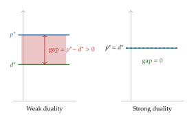
The Lagrange dual problem is $d^{*} = \sup_{λ \geq 0, ν} g (λ, ν)$ . The duality gap is $p^{*} - d^{*} \geq 0$ .

Definition 16 (Strong Duality).

Strong duality holds when the duality gap is zero: $p^{*} = d^{*}$ . Strong duality does not hold in general, but it does hold under mild regularity conditions for convex problems.

Left: weak duality guarantees

d^{*} \leq p^{*}

, but a positive duality gap may remain. Right: under strong duality (e.g. Slater's condition for convex problems), the gap closes and

p^{*} = d^{*}

The fundamental question is: when does strong duality hold? The most widely used sufficient condition for convex problems is Slater's condition.

Definition 17 (Slater's Condition).

For a convex problem (where $f_{0}, f_{1}, \dots, f_{m}$ are convex and $h_{1}, \dots, h_{p}$ are affine), Slater's condition holds if there exists a point $𝒙_{0} \in relint (𝒟)$ such that $f_{i} (𝒙_{0}) < 0, i = 1, \dots, m .$ Such a point $𝒙_{0}$ is called strictly feasible. When some of the inequality constraints $f_{i}$ are affine, the strict inequality is only required for the nonaffine constraints; the affine ones need only satisfy $f_{i} (𝒙_{0}) \leq 0$ .

Theorem 15 (Slater's Theorem).

If the primal problem is convex and Slater's condition holds, then strong duality holds: $p^{*} = d^{*}$ . Furthermore, if $d^{*}$ is finite, the dual optimum is attained.

Proof outline.

Define the set $𝒜 = {(u, v, t) \in ℝ^{m} \times ℝ^{p} \times ℝ : \exists 𝒙 with f_{i} (𝒙) \leq u_{i}, h_{j} (𝒙) = v_{j}, f_{0} (𝒙) \leq t}$ and let $ℬ = {(0,0, s) : s < p^{*}}$ . By convexity of the problem, $𝒜$ is a convex set. The set $ℬ$ is convex (a ray), and $𝒜 \cap ℬ = \emptyset$ (no feasible point achieves an objective value strictly below $p^{*}$ ).

By the separating hyperplane theorem, there exist $(λ, ν, μ) \neq 0$ with $λ \geq 0$ and $μ \geq 0$ such that $λ^{⊤} u + ν^{⊤} v + μ t \geq μ s$ for all $(u, v, t) \in 𝒜$ and all $s < p^{*}$ . Slater's condition ensures that $μ > 0$ : if $μ = 0$ , the strictly feasible point $𝒙_{0}$ leads to a contradiction because the $u$ -coordinates can be made strictly negative while staying in $𝒜$ . Normalising by $μ$ (setting $μ = 1$ ) yields the Lagrange multipliers $(λ, ν)$ for which $g (λ, ν) = p^{*}$ .

∎

Example 8 (Least Squares with Equality Constraints).

Consider $\min_{𝒙} {‖ A 𝒙 - 𝐛 ‖}^{2}$ subject to $C 𝒙 = 𝐝$ . The Lagrangian is $L (𝒙, ν) = {‖ A 𝒙 - 𝐛 ‖}^{2} + ν^{⊤} (C 𝒙 - 𝐝)$ . Setting $\nabla_{𝒙} L = 0$ gives $2 A^{⊤} (A 𝒙 - 𝐛) + C^{⊤} ν = 0$ , so $𝒙^{*} = {(A^{⊤} A)}^{- 1} (A^{⊤} 𝐛 - \frac{1}{2} C^{⊤} ν)$ . Substituting back into the constraint $C 𝒙^{*} = 𝐝$ yields a linear system for $ν^{*}$ . The combined primal-dual system is the familiar KKT system: $(\begin{matrix} 2 A^{⊤} A & C^{⊤} \\ C & 0 \end{matrix}) (\begin{matrix} 𝒙^{*} \\ ν^{*} \end{matrix}) = (\begin{matrix} 2 A^{⊤} 𝐛 \\ 𝐝 \end{matrix}) .$ Since the problem is convex and the constraints are affine, Slater's condition reduces to feasibility: any $𝒙$ with $C 𝒙 = 𝐝$ suffices.

Example 9 (Linear Program Duality).

The linear program $\min_{𝒙} 𝐜^{⊤} 𝒙$ subject to $A 𝒙 = 𝐛$ , $𝒙 \geq 0$ has Lagrangian $L (𝒙, λ, ν) = 𝐜^{⊤} 𝒙 - λ^{⊤} 𝒙 + ν^{⊤} (A 𝒙 - 𝐛)$ with $λ \geq 0$ . The dual function is $g (λ, ν) = \inf_{𝒙 \geq 0} {(𝐜 - λ + A^{⊤} ν)^{⊤} 𝒙 - ν^{⊤} 𝐛} = {\begin{matrix} - 𝐛^{⊤} ν & if A^{⊤} ν + 𝐜 \geq λ \geq 0, \\ - \infty & otherwise . \end{matrix}$ Maximising over $λ$ (which is absorbed by the constraint $A^{⊤} ν \leq 𝐜$ ), the dual LP is: $\max_{ν} 𝐛^{⊤} ν$ subject to $A^{⊤} ν \leq 𝐜$ . Strong duality always holds for LPs whenever the primal is feasible; Slater's condition is not needed because all constraints are affine.

Theorem 16 (Inf-Sup Swap).

For a convex problem with strong duality (e.g. Slater's condition satisfied), (INF SUP) $\begin{matrix} \inf_{𝒙 \in 𝒟} \sup_{λ \geq 0, ν} L (𝒙, λ, ν) = \sup_{λ \geq 0, ν} \inf_{𝒙 \in 𝒟} L (𝒙, λ, ν) . \end{matrix}$

Proof.

Left side equals $p^{*}$ . For a fixed $𝒙$ , consider the inner supremum over $(λ \geq 0, ν)$ . If $𝒙$ violates any inequality constraint $f_{i} (𝒙) > 0$ , setting $λ_{i} \to \infty$ makes the supremum $+ \infty$ . If $𝒙$ violates any equality constraint $h_{j} (𝒙) \neq 0$ , sending $ν_{j} \to \pm \infty$ likewise gives $+ \infty$ . If $𝒙$ is feasible, the optimal choice is $λ = 0$ (since $λ_{i} f_{i} (𝒙) \leq 0$ when $λ_{i} \geq 0$ and $f_{i} (𝒙) \leq 0$ ), yielding $L (𝒙, 0, ν) = f_{0} (𝒙)$ (the $h_{j}$ terms vanish). Therefore $\sup_{λ \geq 0, ν} L (𝒙, λ, ν) = {\begin{matrix} f_{0} (𝒙) & if 𝒙 is feasible, \\ + \infty & otherwise. \end{matrix}$ Taking the infimum over $𝒙$ gives $p^{*}$ .

Right side equals $d^{*}$ . The inner infimum $\inf_{𝒙} L (𝒙, λ, ν) = g (λ, ν)$ by definition. The outer supremum is $\sup_{λ \geq 0, ν} g (λ, ν) = d^{*}$ .

Conclusion. Strong duality gives $p^{*} = d^{*}$ , completing the proof.

∎

Key Idea.

The Kantorovich–Rubinstein duality for the Wasserstein-1 distance is a direct application of this machinery. The primal problem is: minimise $𝔼_{π} [‖ 𝒙 - 𝒚 ‖]$ over couplings $π$ with marginals $P$ and $Q$ . This is a linear program (linear objective, affine marginal constraints). Slater's condition holds trivially: the product measure $P \times Q$ is strictly feasible. Strong duality then swaps $\inf$ and $\sup$ , yielding the dual: $W_{1} (P, Q) = \sup_{{‖ f ‖}_{L} \leq 1} {𝔼_{P} [f (𝒙)] - 𝔼_{Q} [f (𝒙)]},$ which is precisely what the WGAN critic network optimises.

KKT Conditions

The Karush–Kuhn–Tucker (KKT) conditions are the most important optimality conditions in constrained optimisation. For convex problems with strong duality, they provide necessary and sufficient conditions for a point to be optimal. In machine learning, KKT conditions characterise the optimal solutions of support vector machines, constrained optimisation in normalising flows, and optimal transport problems.

Theorem 17 (KKT Conditions).

Consider a convex problem with all functions differentiable. If strong duality holds, then $𝒙^{*}$ is primal optimal and $(λ^{*}, ν^{*})$ is dual optimal if and only if the following four conditions hold simultaneously:

Primal feasibility:; $f_{i} (𝒙^{*}) \leq 0$ for all $i$ ;; $h_{j} (𝒙^{*}) = 0$ for all $j$ .
Dual feasibility:; $λ_{i}^{*} \geq 0$ for all $i$ .
Complementary slackness:; $λ_{i}^{*} f_{i} (𝒙^{*}) = 0$ for all $i$ .
Stationarity:; $\nabla f_{0} (𝒙^{*}) + \sum_{i = 1}^{m} λ_{i}^{*} \nabla f_{i} (𝒙^{*}) + \sum_{j = 1}^{p} ν_{j}^{*} \nabla h_{j} (𝒙^{*}) = 0$ .

Proof.

Sufficiency (for convex problems). Suppose the four conditions hold and the problem is convex. Because all $f_{i}$ are convex, $L (\cdot, λ^{*}, ν^{*})$ is convex in $𝒙$ . Stationarity (iv) says that $\nabla_{𝒙} L (𝒙^{*}, λ^{*}, ν^{*}) = 0$ , so $𝒙^{*}$ minimises $L (\cdot, λ^{*}, ν^{*})$ . Therefore $\begin{matrix} g (λ^{*}, ν^{*}) & = \inf_{𝒙} L (𝒙, λ^{*}, ν^{*}) = L (𝒙^{*}, λ^{*}, ν^{*}) \\ = f_{0} (𝒙^{*}) + \sum_{i} λ_{i}^{*} f_{i} (𝒙^{*}) + \sum_{j} ν_{j}^{*} h_{j} (𝒙^{*}) \\ = f_{0} (𝒙^{*}) + 0 + 0 = f_{0} (𝒙^{*}), \end{matrix}$ where the penultimate step uses complementary slackness (iii) and primal feasibility (i). Hence $d^{*} \geq g (λ^{*}, ν^{*}) = f_{0} (𝒙^{*}) \geq p^{*}$ . Combined with weak duality $d^{*} \leq p^{*}$ , we conclude $p^{*} = d^{*} = f_{0} (𝒙^{*})$ , so $𝒙^{*}$ is primal optimal and $(λ^{*}, ν^{*})$ is dual optimal.

Necessity (under strong duality). Suppose $𝒙^{*}$ is primal optimal and $(λ^{*}, ν^{*})$ is dual optimal with $p^{*} = d^{*}$ . Dual feasibility (ii) is part of the dual constraints. Primal feasibility (i) holds by assumption. We have $\begin{matrix} f_{0} (𝒙^{*}) & = p^{*} = d^{*} = g (λ^{*}, ν^{*}) = \inf_{𝒙} L (𝒙, λ^{*}, ν^{*}) \\ \leq L (𝒙^{*}, λ^{*}, ν^{*}) = f_{0} (𝒙^{*}) + \sum_{i} λ_{i}^{*} f_{i} (𝒙^{*}) . \end{matrix}$ Since $λ_{i}^{*} \geq 0$ and $f_{i} (𝒙^{*}) \leq 0$ , each term $λ_{i}^{*} f_{i} (𝒙^{*}) \leq 0$ . The inequality above forces the sum to be zero, which requires every term to vanish: $λ_{i}^{*} f_{i} (𝒙^{*}) = 0$ for all $i$ (complementary slackness). Additionally, the inequality $\inf_{𝒙} L (𝒙, λ^{*}, ν^{*}) \leq L (𝒙^{*}, λ^{*}, ν^{*})$ must hold with equality, so $𝒙^{*}$ is a minimiser of $L (\cdot, λ^{*}, ν^{*})$ . Since $L$ is differentiable, this gives $\nabla_{𝒙} L (𝒙^{*}, λ^{*}, ν^{*}) = 0$ (stationarity).

∎

Remark 3 (Complementary Slackness Interpretation).

The condition $λ_{i}^{*} f_{i} (𝒙^{*}) = 0$ has a clean interpretation. For each inequality constraint, exactly one of two situations occurs:

The constraint is inactive: $f_{i} (𝒙^{*}) < 0$ , meaning the constraint is slack. Then $λ_{i}^{*} = 0$ , so the constraint does not affect the optimal solution.
The constraint is active: $f_{i} (𝒙^{*}) = 0$ , meaning the constraint is tight. Then $λ_{i}^{*}$ may be positive, reflecting the “price” of tightening the constraint.

In economic terms, $λ_{i}^{*}$ is the shadow price: it measures how much the optimal objective would improve if the $i$ -th constraint were relaxed by an infinitesimal amount.

KKT conditions in two dimensions. The contour lines of the objective

f_{0}

(blue ellipses) meet the constraint boundary

f_{1} (𝒙) = 0

(red curve) at the optimum

𝒙^{*}

(green dot). The negative gradient of

f_{0}

(solid orange) and the gradient of

f_{1}

(dashed orange) are antiparallel, reflecting the stationarity condition

\nabla f_{0} (𝒙^{*}) + λ_{1}^{*} \nabla f_{1} (𝒙^{*}) = 0

with

λ_{1}^{*} > 0

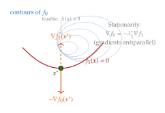
Example 10 (Water-Filling Power Allocation).

Consider the power allocation problem: distribute a total power budget $B$ across $n$ channels to maximise total capacity. In convex-minimisation form: $\min_{𝒙} - \sum_{i = 1}^{n} \log (x_{i} + a_{i}) s.t. x_{i} \geq 0, \sum_{i = 1}^{n} x_{i} = B,$ where $a_{i} > 0$ is the noise level in channel $i$ . The KKT stationarity condition with multiplier $ν$ for the equality constraint and $μ_{i} \geq 0$ for $- x_{i} \leq 0$ gives $- \frac{1}{x_{i} + a_{i}} + ν - μ_{i} = 0, μ_{i} x_{i} = 0.$ If $x_{i} > 0$ , then $μ_{i} = 0$ and $x_{i} = 1 / ν - a_{i}$ . If $1 / ν - a_{i} \leq 0$ , then $x_{i} = 0$ . The resulting water-filling solution is (Water Filling) $\begin{matrix} x_{i}^{*} = \max (0, \frac{1}{ν} - a_{i}), \end{matrix}$ where $ν > 0$ is chosen so that $\sum_{i} x_{i}^{*} = B$ . The name “water-filling” comes from imagining the $a_{i}$ as the bottoms of containers of varying depth: pouring water (power) fills from the shallowest container first, with the water level $1 / ν$ uniform across all active channels.

Historical Note.

William Karush derived these optimality conditions in his 1939 master's thesis at the University of Chicago, but the work went largely unnoticed. Harold Kuhn and Albert Tucker independently rediscovered them in 1951, publishing the result in the proceedings of the Second Berkeley Symposium. For decades the conditions were known as the “Kuhn–Tucker conditions” until Karush's priority was recognised in the 1970s through the efforts of historians of optimisation. This is one of many examples in mathematics where graduate student work was overshadowed by more established researchers, a pattern that, happily, the modern culture of open preprints and arxiv has done much to correct.

Minimax Problems and Saddle Points

Generative adversarial networks are fundamentally minimax problems: the generator minimises while the discriminator maximises the same objective. Understanding when $\min \max = \max \min$ , and when saddle points exist, is therefore directly relevant to understanding when and why GANs converge. This section develops the classical theory of minimax problems and saddle points, beginning with the definition of a saddle point and culminating in the Von Neumann minimax theorem and its implications for adversarial training.

Definition 18 (Saddle Point).

Let $X \subseteq ℝ^{n}$ , $Y \subseteq ℝ^{m}$ , and let $f : X \times Y \to ℝ$ . A pair $(𝒙^{*}, 𝒚^{*}) \in X \times Y$ is a saddle point of $f$ if (Saddle DEF) $\begin{matrix} f (𝒙^{*}, 𝒚) \leq f (𝒙^{*}, 𝒚^{*}) \leq f (𝒙, 𝒚^{*}) for all 𝒙 \in X, 𝒚 \in Y . \end{matrix}$ Equivalently, $𝒙^{*}$ minimises $f (\cdot, 𝒚^{*})$ over $X$ and $𝒚^{*}$ maximises $f (𝒙^{*}, \cdot)$ over $Y$ . Geometrically, the graph of $f$ curves upward in the $𝒙$ -direction and downward in the $𝒚$ -direction at the saddle point, resembling a horse saddle.

Theorem 18 (Minimax Inequality).

For any function $f : X \times Y \to ℝ$ , (Minimax INEQ) $\begin{matrix} \sup_{𝒚 \in Y} \inf_{𝒙 \in X} f (𝒙, 𝒚) \leq \inf_{𝒙 \in X} \sup_{𝒚 \in Y} f (𝒙, 𝒚) . \end{matrix}$ The left-hand side is called the maximin value and the right-hand side the minimax value. The inequality states that the best guaranteed payoff for the maximiser (who moves first) is at most the worst-case cost for the minimiser (who moves first).

Proof.

Fix an arbitrary $𝒚_{0} \in Y$ . For every $𝒙 \in X$ we have $\inf_{𝒙^{'} \in X} f (𝒙^{'}, 𝒚_{0}) \leq f (𝒙, 𝒚_{0}) \leq \sup_{𝒚 \in Y} f (𝒙, 𝒚) .$ The left inequality holds because the infimum is a lower bound, and the right inequality holds because the supremum is an upper bound. Since the rightmost expression does not depend on $𝒚_{0}$ , we take the infimum over $𝒙$ on the right: $\inf_{𝒙^{'} \in X} f (𝒙^{'}, 𝒚_{0}) \leq \inf_{𝒙 \in X} \sup_{𝒚 \in Y} f (𝒙, 𝒚) .$ Since this holds for every $𝒚_{0} \in Y$ , we may take the supremum over $𝒚_{0}$ on the left to obtain the desired inequality.

∎

Theorem 19 (Saddle Point Implies Minimax Equality).

If $(𝒙^{*}, 𝒚^{*})$ is a saddle point of $f : X \times Y \to ℝ$ , then the minimax value equals the maximin value and both equal $f (𝒙^{*}, 𝒚^{*})$ : (Saddle Minimax) $\begin{matrix} \min_{𝒙 \in X} \max_{𝒚 \in Y} f (𝒙, 𝒚) = \max_{𝒚 \in Y} \min_{𝒙 \in X} f (𝒙, 𝒚) = f (𝒙^{*}, 𝒚^{*}) . \end{matrix}$

Proof.

Since $𝒚^{*}$ maximises $f (𝒙^{*}, \cdot)$ , we have $f (𝒙^{*}, 𝒚^{*}) = \max_{𝒚} f (𝒙^{*}, 𝒚)$ . Bounding the outer minimisation by its value at $𝒙 = 𝒙^{*}$ , $\min_{𝒙} \max_{𝒚} f (𝒙, 𝒚) \leq \max_{𝒚} f (𝒙^{*}, 𝒚) = f (𝒙^{*}, 𝒚^{*}) .$ Similarly, since $𝒙^{*}$ minimises $f (\cdot, 𝒚^{*})$ , we have $f (𝒙^{*}, 𝒚^{*}) = \min_{𝒙} f (𝒙, 𝒚^{*})$ . Bounding the outer maximisation by its value at $𝒚 = 𝒚^{*}$ , $\max_{𝒚} \min_{𝒙} f (𝒙, 𝒚) \geq \min_{𝒙} f (𝒙, 𝒚^{*}) = f (𝒙^{*}, 𝒚^{*}) .$ Combining these two bounds with the minimax inequality (Theorem 18), $f (𝒙^{*}, 𝒚^{*}) \geq \min_{𝒙} \max_{𝒚} f (𝒙, 𝒚) \geq \max_{𝒚} \min_{𝒙} f (𝒙, 𝒚) \geq f (𝒙^{*}, 𝒚^{*}),$ so all three quantities are equal.

∎

Theorem 20 (Von Neumann Minimax Theorem).

Let $X \subseteq ℝ^{n}$ and $Y \subseteq ℝ^{m}$ be compact convex sets, and let $f : X \times Y \to ℝ$ be continuous such that

$f (\cdot, 𝒚)$ is convex for each fixed $𝒚 \in Y$ , and
$f (𝒙, \cdot)$ is concave for each fixed $𝒙 \in X$ .

Then: (VON Neumann) $\begin{matrix} \min_{𝒙 \in X} \max_{𝒚 \in Y} f (𝒙, 𝒚) = \max_{𝒚 \in Y} \min_{𝒙 \in X} f (𝒙, 𝒚), \end{matrix}$ and a saddle point $(𝒙^{*}, 𝒚^{*})$ exists.

Proof.

We give a sketch that highlights the key ideas. Define $φ (𝒙) = \max_{𝒚 \in Y} f (𝒙, 𝒚)$ . Since $f (𝒙, \cdot)$ is concave and $Y$ is compact, the maximum is attained for every $𝒙$ . Moreover, $φ$ is convex: for any $𝒙_{1}, 𝒙_{2} \in X$ and $λ \in [0,1]$ , $φ (λ 𝒙_{1} + (1 - λ) 𝒙_{2}) = \max_{𝒚} f (λ 𝒙_{1} + (1 - λ) 𝒙_{2}, 𝒚) \leq \max_{𝒚} [λ f (𝒙_{1}, 𝒚) + (1 - λ) f (𝒙_{2}, 𝒚)] \leq λ φ (𝒙_{1}) + (1 - λ) φ (𝒙_{2}),$ using the convexity of $f$ in $𝒙$ . Since $φ$ is continuous and convex on the compact set $X$ , it attains its minimum at some $𝒙^{*} \in X$ . Similarly, define $ψ (𝒚) = \min_{𝒙 \in X} f (𝒙, 𝒚)$ , which is concave and attains its maximum at some $𝒚^{*} \in Y$ .

By the minimax inequality (Theorem 18), $ψ (𝒚^{*}) \leq φ (𝒙^{*})$ . The convex-concave structure of $f$ can be used, via a separating hyperplane argument on the epigraphs, to show that $φ (𝒙^{*}) \leq ψ (𝒚^{*})$ as well. It follows that $f (𝒙^{*}, 𝒚^{*})$ is a saddle point, and the minimax and maximin values coincide.

∎

Definition 19 (Nash Equilibrium).

In a two-player zero-sum game with payoff $f (𝒙, 𝒚)$ , a Nash equilibrium is a pair $(𝒙^{*}, 𝒚^{*})$ such that no player can improve their payoff by unilaterally changing their strategy: $f (𝒙^{*}, 𝒚) \leq f (𝒙^{*}, 𝒚^{*}) \leq f (𝒙, 𝒚^{*}) for all 𝒙 \in X, 𝒚 \in Y .$ For zero-sum games, Nash equilibria coincide exactly with saddle points.

Key Idea.

The original GAN solves $\min_{G} \max_{D} V (G, D)$ where $V$ is concave in $D$ (a sum of logarithms of $D$ and $1 - D$ ) but highly non-convex in $G$ (since $G$ is parameterised by a deep neural network). The Von Neumann minimax theorem does not apply, which is precisely why GAN training is unstable. The minimax inequality $\max_{D} \min_{G} V \leq \min_{G} \max_{D} V$ may be strict: the “generator-first” game and the “discriminator-first” game can have different values.

WGANs, spectral normalisation, and gradient penalties are all designed to bring the GAN objective closer to the convex-concave setting where minimax theory guarantees convergence. When the GAN objective is re-parameterised in distribution space (rather than parameter space), the optimal discriminator yields an objective that is convex in the generator's distribution $p_{g}$ , partially recovering the conditions of the Von Neumann theorem.

Example 11 (Bilinear Saddle Point).

Consider $f (𝒙, 𝒚) = 𝒙^{⊤} A 𝒚$ on compact convex sets $X \subseteq ℝ^{n}$ and $Y \subseteq ℝ^{m}$ , where $A \in ℝ^{n \times m}$ . For fixed $𝒚$ , $f$ is linear (hence convex) in $𝒙$ ; for fixed $𝒙$ , $f$ is linear (hence concave) in $𝒚$ . The Von Neumann theorem applies, and a saddle point exists.

This bilinear game is the simplest model of a GAN-like adversarial problem. When $X$ and $Y$ are simplices (probability vectors), the game becomes a matrix game, and the saddle-point strategies are mixed Nash equilibria. Gradient descent-ascent on bilinear objectives oscillates without converging, which foreshadows the training instabilities observed in GANs.

Historical Note.

John von Neumann proved his minimax theorem in 1928 as part of his foundational work on game theory, which he later expanded with Oskar Morgenstern in their 1944 book Theory of Games and Economic Behavior. Maurice Sion generalised the theorem to quasi-convex/quasi-concave functions in 1958, weakening the linearity assumptions considerably. The connection to generative modelling was made explicit by Goodfellow et al. (2014), who showed that the optimal discriminator yields a convex-in- $p_{g}$ objective when viewed in distribution space, partially recovering the minimax setting.

Bregman Divergences

Bregman divergences generalise the notion of “distance” beyond Euclidean distance, using a convex function to define a measure of dissimilarity. They arise naturally in information geometry, entropic optimal transport, and mirror descent algorithms. In generative modelling, the Sinkhorn algorithm for optimal transport is elegantly understood as alternating Bregman projections, and the KL divergence, the central quantity in variational inference, is itself a Bregman divergence.

Definition 20 (Bregman Divergence).

Let $φ : ℝ^{n} \to ℝ$ be a strictly convex, differentiable function. The Bregman divergence associated with $φ$ is (Bregman DEF) $\begin{matrix} D_{φ} (𝒙, 𝒚) = φ (𝒙) - φ (𝒚) - \nabla φ {(𝒚)}^{⊤} (𝒙 - 𝒚) . \end{matrix}$ Intuitively, $D_{φ} (𝒙, 𝒚)$ measures the gap between $φ (𝒙)$ and its first-order Taylor approximation centred at $𝒚$ , evaluated at $𝒙$ .

Theorem 21 (Non-Negativity).

$D_{φ} (𝒙, 𝒚) \geq 0$ for all $𝒙, 𝒚$ , with equality if and only if $𝒙 = 𝒚$ .

Proof.

By the first-order condition for strict convexity of $φ$ : $φ (𝒙) > φ (𝒚) + \nabla φ {(𝒚)}^{⊤} (𝒙 - 𝒚) whenever 𝒙 \neq 𝒚 .$ Rearranging gives $D_{φ} (𝒙, 𝒚) > 0$ when $𝒙 \neq 𝒚$ . When $𝒙 = 𝒚$ , we have $D_{φ} (𝒙, 𝒙) = φ (𝒙) - φ (𝒙) - 0 = 0$ trivially.

∎

The Bregman divergence

D_{φ} (𝒙, 𝒚)

is the vertical gap between the strictly convex function

φ

(blue) and its tangent line at

𝒚

(orange dashed), evaluated at

𝒙

. The gap (red) is always non-negative by the first-order convexity condition.

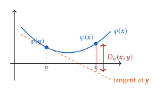
Remark 4 (Bregman Divergence Is Not a Metric).

Despite its name, $D_{φ}$ is not a metric in general. It is typically asymmetric ( $D_{φ} (𝒙, 𝒚) \neq D_{φ} (𝒚, 𝒙)$ ) and does not satisfy the triangle inequality. The term “divergence” is used deliberately to distinguish it from a true distance. The asymmetry is not a defect but a feature: it allows Bregman divergences to encode directional information about the curvature of $φ$ .

Example 12 (Squared Euclidean Distance).

Let $φ (𝒙) = \frac{1}{2} {‖ 𝒙 ‖}^{2}$ . Then $\nabla φ (𝒚) = 𝒚$ and $D_{φ} (𝒙, 𝒚) = \frac{1}{2} {‖ 𝒙 ‖}^{2} - \frac{1}{2} {‖ 𝒚 ‖}^{2} - 𝒚^{⊤} (𝒙 - 𝒚) = \frac{1}{2} {‖ 𝒙 - 𝒚 ‖}^{2} .$ This is the unique Bregman divergence that is symmetric and satisfies the triangle inequality. It is both a Bregman divergence and a squared metric.

Example 13 (KL Divergence).

Let $φ (𝒑) = \sum_{i} p_{i} \log p_{i}$ (the negative entropy) defined on the probability simplex. Then $\nabla φ (𝒒) = {(\log q_{i} + 1)}_{i}$ and $D_{φ} (𝒑, 𝒒) = \sum_{i} p_{i} \log p_{i} - \sum_{i} q_{i} \log q_{i} - \sum_{i} (\log q_{i} + 1) (p_{i} - q_{i}) = \sum_{i} p_{i} \log \frac{p_{i}}{q_{i}} = KL (𝒑 ‖ 𝒒) .$ This reveals that the KL divergence is a Bregman divergence, which immediately explains its asymmetry: $KL (𝒑 ‖ 𝒒) \neq KL (𝒒 ‖ 𝒑)$ in general.

Example 14 (Itakura–Saito Distance).

Let $φ (𝒙) = - \sum_{i} \log x_{i}$ on $ℝ_{+ +}^{n}$ . Then $D_{φ} (𝒙, 𝒚) = \sum_{i} (\frac{x_{i}}{y_{i}} - \log \frac{x_{i}}{y_{i}} - 1) .$ This divergence is scale-invariant and appears in audio signal processing, where it measures spectral distortion between power spectra.

Definition 21 (Bregman Projection).

The Bregman projection of a point $𝒙$ onto a closed convex set $C$ with respect to $φ$ is (Bregman PROJ) $\begin{matrix} π_{C}^{φ} (𝒙) = {arg min}_{𝒚 \in C} D_{φ} (𝒚, 𝒙) . \end{matrix}$ When $φ = \frac{1}{2} {‖ \cdot ‖}^{2}$ , this reduces to the standard Euclidean projection $Π_{C} (𝒙) = {arg min}_{𝒚 \in C} {‖ 𝒚 - 𝒙 ‖}^{2}$ .

Key Idea.

The Sinkhorn algorithm for entropic optimal transport can be understood as alternating Bregman projections with $φ$ equal to the negative entropy, giving KL divergence as the Bregman divergence. The two constraint sets are:

$C_{1} = {π \geq 0 : π 𝟙 = 𝒑}$ (row marginals match $P$ ), and
$C_{2} = {π \geq 0 : π^{⊤} 𝟙 = 𝒒}$ (column marginals match $Q$ ).

Each Sinkhorn iteration projects onto one constraint, then the other, by rescaling the rows and columns of the coupling matrix. The theory of alternating Bregman projections guarantees convergence to the unique point in $C_{1} \cap C_{2}$ that minimises the KL divergence from the initial coupling, which is precisely the entropy-regularised optimal transport plan.

Proximal Operators

Proximal operators provide a principled way to handle non-smooth terms in optimisation by combining a gradient-like step with a regularisation penalty. They are the building blocks of modern first-order methods for composite optimisation problems of the form $\min_{𝒙} g (𝒙) + f (𝒙)$ , where $g$ is smooth and $f$ may be non-differentiable.

Definition 22 (Proximal Operator).

For a closed, proper, convex function $f : ℝ^{n} \to ℝ \cup {+ \infty}$ , the proximal operator of $f$ is the mapping ${prox}_{f} : ℝ^{n} \to ℝ^{n}$ defined by (PROX DEF) $\begin{matrix} {prox}_{f} (𝒗) = {arg min}_{𝒙 \in ℝ^{n}} {f (𝒙) + \frac{1}{2} {‖ 𝒙 - 𝒗 ‖}^{2}} . \end{matrix}$ The minimiser always exists and is unique because the objective is the sum of a convex function and a strictly convex quadratic, making it strongly convex. Intuitively, ${prox}_{f} (𝒗)$ finds the point that balances being close to $𝒗$ (the quadratic term) with having small $f$ -value (the penalty term).

Theorem 22 (Proximal Operator is Firmly Non-Expansive).

For any closed convex $f$ , the proximal operator satisfies: (PROX FIRM) $\begin{matrix} {‖ {prox}_{f} (𝒙) - {prox}_{f} (𝒚) ‖}^{2} \leq (𝒙 - 𝒚)^{⊤} ({prox}_{f} (𝒙) - {prox}_{f} (𝒚)) \end{matrix}$ for all $𝒙, 𝒚 \in ℝ^{n}$ . In particular, $‖ {prox}_{f} (𝒙) - {prox}_{f} (𝒚) ‖ \leq ‖ 𝒙 - 𝒚 ‖$ (non-expansiveness).

Proof.

Let $𝒖 = {prox}_{f} (𝒙)$ and $𝒘 = {prox}_{f} (𝒚)$ . By the optimality condition for (PROX DEF), we have $𝒙 - 𝒖 \in \partial f (𝒖)$ and $𝒚 - 𝒘 \in \partial f (𝒘)$ . By the monotonicity of the subdifferential of a convex function (if $𝒔_{1} \in \partial f (𝒖)$ and $𝒔_{2} \in \partial f (𝒘)$ , then ${(𝒔_{1} - 𝒔_{2})}^{⊤} (𝒖 - 𝒘) \geq 0$ ), we obtain: $((𝒙 - 𝒖) - (𝒚 - 𝒘))^{⊤} (𝒖 - 𝒘) \geq 0.$ Expanding gives ${(𝒙 - 𝒚)}^{⊤} (𝒖 - 𝒘) - {‖ 𝒖 - 𝒘 ‖}^{2} \geq 0$ , which rearranges to the stated inequality. The non-expansiveness follows by applying the Cauchy–Schwarz inequality to the right-hand side.

∎

Example 15 (Proximal of $ℓ_{1}$ Norm: Soft-Thresholding).

For $f (𝒙) = λ {‖ 𝒙 ‖}_{1}$ with $λ > 0$ , the proximal operator acts component-wise via soft-thresholding: (SOFT Threshold) $\begin{matrix} ({prox}_{f} (𝒗))_{i} = sign (v_{i}) \max (| v_{i} | - λ, 0) . \end{matrix}$ This operator shrinks each component of $𝒗$ towards zero by $λ$ , setting small components exactly to zero. It is the key step in LASSO regression and compressed sensing for promoting sparsity.

Example 16 (Proximal of Indicator Function: Projection).

For the indicator function $f = I_{C}$ of a closed convex set $C$ (i.e., $f (𝒙) = 0$ if $𝒙 \in C$ and $f (𝒙) = + \infty$ otherwise), the proximal operator reduces to the Euclidean projection: ${prox}_{I_{C}} (𝒗) = Π_{C} (𝒗) = {arg min}_{𝒙 \in C} {‖ 𝒙 - 𝒗 ‖}^{2} .$ This shows that projection is a special case of the proximal operator, and all results for proximal operators (such as non-expansiveness) immediately apply to projections.

Theorem 23 (Moreau Decomposition).

For any closed proper convex function $f$ and any $𝒗 \in ℝ^{n}$ : (Moreau) $\begin{matrix} 𝒗 = {prox}_{f} (𝒗) + {prox}_{f^{*}} (𝒗), \end{matrix}$ where $f^{*}$ is the Fenchel conjugate of $f$ . This decomposes every vector $𝒗$ into a “primal” component ${prox}_{f} (𝒗)$ and a “dual” component ${prox}_{f^{*}} (𝒗)$ .

Remark 5 (Interpretation of the Moreau Decomposition).

When $f = I_{C}$ is the indicator of a closed convex set $C$ , we have ${prox}_{f} (𝒗) = Π_{C} (𝒗)$ and ${prox}_{f^{*}} (𝒗) = 𝒗 - Π_{C} (𝒗)$ , which is the residual after projection. The conjugate $f^{*} = σ_{C}$ is the support function of $C$ , and its proximal operator extracts the component of $𝒗$ that “points away” from $C$ . The decomposition $𝒗 = Π_{C} (𝒗) + (𝒗 - Π_{C} (𝒗))$ is the familiar orthogonal decomposition in the Euclidean case.

Remark 6 (Proximal Gradient Methods).

For problems of the form $\min_{𝒙} g (𝒙) + f (𝒙)$ , where $g$ is smooth with Lipschitz-continuous gradient and $f$ is convex but possibly non-smooth with an inexpensive proximal operator, the proximal gradient method iterates: (PROX GRAD) $\begin{matrix} 𝒙_{k + 1} = {prox}_{t_{k} f} (𝒙_{k} - t_{k} \nabla g (𝒙_{k})), \end{matrix}$ where $t_{k} > 0$ is the step size. Each iteration alternates a gradient step on $g$ with a proximal step on $f$ . With step size $t_{k} = 1 / L$ (where $L$ is the Lipschitz constant of $\nabla g$ ), the method achieves an $O (1 / k)$ convergence rate. Accelerated variants such as FISTA (Fast Iterative Shrinkage-Thresholding Algorithm) achieve the optimal $O (1 / k^{2})$ rate among first-order methods.

In generative modelling, the denoising step in DDPM can be interpreted as a proximal-like operation: given a noisy observation, the learned denoiser finds the closest clean signal under the learned prior, balancing data fidelity (proximity to the noisy input) with prior plausibility (the regularisation term).

Exercises

Convex Sets and Functions ( B.1–B.2)

Exercise 1 (Intersection of Convex Sets).

Let ${C_{α}}_{α \in A}$ be an arbitrary family of convex subsets of $ℝ^{n}$ . Prove that the intersection $⋂_{α \in A} C_{α}$ is convex. Give an example showing that the union of two convex sets need not be convex.

Exercise 2 (Convexity Preserved Under Affine Composition).

Let $f : ℝ^{m} \to ℝ$ be convex and let $g : ℝ^{n} \to ℝ^{m}$ be affine, i.e., $g (𝒙) = A 𝒙 + 𝒃$ for some matrix $A$ and vector $𝒃$ . Prove that $h = f \circ g$ is convex.

Hint: Use the definition of convexity directly and the affinity of $g$ .

Exercise 3 (Jensen's Inequality).

Let $f : ℝ^{n} \to ℝ$ be convex and let $X$ be a random variable with $𝔼 [X]$ finite and $𝔼 [X] \in dom f$ . Prove that (Jensen EX) $\begin{matrix} f (𝔼 [X]) \leq 𝔼 [f (X)] . \end{matrix}$ Hint: By the supporting hyperplane characterisation of convexity, for any $𝒙_{0} \in dom f$ there exists a subgradient $𝒈 \in \partial f (𝒙_{0})$ such that $f (𝒙) \geq f (𝒙_{0}) + 𝒈^{⊤} (𝒙 - 𝒙_{0})$ for all $𝒙$ . Choose $𝒙_{0} = 𝔼 [X]$ and take expectations.

Subgradients ( B.3)

Exercise 4 (Subdifferential of the Max Function).

Let $f (𝒙) = \max (x_{1}, x_{2}, \dots, x_{n})$ for $𝒙 \in ℝ^{n}$ . At a point $𝒙$ where exactly $k$ coordinates achieve the maximum (i.e., $x_{i_{1}} = x_{i_{2}} = \dots = x_{i_{k}} = \max_{j} x_{j}$ ), show that the subdifferential is $\partial f (𝒙) = conv {𝒆_{i_{1}}, 𝒆_{i_{2}}, \dots, 𝒆_{i_{k}}},$ where $𝒆_{i}$ denotes the $i$ -th standard basis vector.

Exercise 5 (Subdifferential of the Euclidean Norm).

Let $f (𝒙) = {‖ 𝒙 ‖}_{2}$ for $𝒙 \in ℝ^{n}$ . Show that:

For $𝒙 \neq 0$ : $\partial f (𝒙) = {𝒙 / {‖ 𝒙 ‖}_{2}}$ (a singleton).
At $𝒙 = 0$ : $\partial f (0) = {𝒈 \in ℝ^{n} : {‖ 𝒈 ‖}_{2} \leq 1}$ (the closed unit ball).

Conjugate Functions ( B.5)

Exercise 6 (Conjugate of the Euclidean Norm).

Prove that the Fenchel conjugate of $f (𝒙) = {‖ 𝒙 ‖}_{2}$ is the indicator function of the unit ball: $f^{*} (𝒚) = I_{{{‖ 𝒚 ‖}_{2} \leq 1}} (𝒚) = {\begin{matrix} 0 & if {‖ 𝒚 ‖}_{2} \leq 1, \\ + \infty & otherwise . \end{matrix}$ Hint: Compute $\sup_{𝒙} (𝒚^{⊤} 𝒙 - {‖ 𝒙 ‖}_{2})$ by considering the Cauchy–Schwarz inequality and analysing the cases ${‖ 𝒚 ‖}_{2} \leq 1$ and ${‖ 𝒚 ‖}_{2} > 1$ separately.

Exercise 7 (Conjugate of Log-Sum-Exp).

Consider the log-sum-exp function $f (𝒙) = \log (\sum_{i = 1}^{n} e^{x_{i}})$ . Compute its conjugate $f^{*} (𝒚)$ and show that $f^{*} (𝒚) = {\begin{matrix} \sum_{i = 1}^{n} y_{i} \log y_{i} & if 𝒚 \in Δ_{n}, \\ + \infty & otherwise, \end{matrix}$ where $Δ_{n} = {𝒚 \in ℝ_{+}^{n} : \sum_{i} y_{i} = 1}$ is the probability simplex. This shows that the conjugate of log-sum-exp is the negative entropy restricted to the simplex.

Hint: Differentiate $𝒚^{⊤} 𝒙 - f (𝒙)$ with respect to $𝒙$ and use the fact that the softmax function arises as the gradient of log-sum-exp.

Exercise 8 (Conjugate of a Quadratic).

Let $f (𝒙) = \frac{1}{2} 𝒙^{⊤} Q 𝒙$ where $Q ≻ 0$ (positive definite).

Compute $f^{*} (𝒚)$ and show that $f^{*} (𝒚) = \frac{1}{2} 𝒚^{⊤} Q^{- 1} 𝒚$ .
Verify the biconjugate identity: $f^{* *} (𝒙) = f (𝒙)$ .

Duality and KKT Conditions ( B.6–B.7)

Exercise 9 (Dual of a Standard-Form Linear Program).

Consider the LP in standard form: $\min_{𝒙} 𝒄^{⊤} 𝒙 s.t. A 𝒙 \leq 𝒃, 𝒙 \geq 0 .$ Write the Lagrangian, compute the dual function, and show that the dual problem is: $\max_{𝝀} 𝒃^{⊤} 𝝀 s.t. A^{⊤} 𝝀 \geq 𝒄, 𝝀 \leq 0 .$ Note: Equivalently, with the sign convention $𝝁 = - 𝝀 \geq 0$ , the dual becomes $\max_{𝝁} - 𝒃^{⊤} 𝝁$ subject to $A^{⊤} 𝝁 \leq 𝒄, 𝝁 \geq 0$ .

Exercise 10 (Slater's Condition for Optimal Transport).

The Kantorovich primal problem for Wasserstein-1 distance is $\min_{π \in Π (P, Q)} \int ‖ 𝒙 - 𝒚 ‖ d π (𝒙, 𝒚),$ where $Π (P, Q)$ is the set of couplings with marginals $P$ and $Q$ . This is a linear program over the convex set $Π (P, Q)$ .

Verify that the product coupling $π = P \times Q$ belongs to $Π (P, Q)$ , and explain why Slater's condition is automatically satisfied for this LP (since all constraints are affine). Conclude that strong duality holds.

Exercise 11 (KKT Conditions for Constrained Least Norm).

Consider the optimisation problem: $\min_{𝒙 \in ℝ^{n}} {‖ 𝒙 ‖}^{2} s.t. A 𝒙 = 𝒃,$ where $A \in ℝ^{p \times n}$ has full row rank and $𝒃 \in ℝ^{p}$ .

Write the Lagrangian $L (𝒙, 𝝂)$ and derive the KKT conditions.
Show that the KKT conditions yield the closed-form solution $𝒙^{*} = A^{⊤} {(A A^{⊤})}^{- 1} 𝒃$ .
Verify that $𝒙^{*}$ is the minimum-norm solution of $A 𝒙 = 𝒃$ (the Moore–Penrose pseudoinverse solution).

Minimax Problems ( B.8)

Exercise 12 (Proving the Minimax Inequality).

Let $f : X \times Y \to ℝ$ be an arbitrary function. Prove directly from the definitions of supremum and infimum that $\sup_{𝒚 \in Y} \inf_{𝒙 \in X} f (𝒙, 𝒚) \leq \inf_{𝒙 \in X} \sup_{𝒚 \in Y} f (𝒙, 𝒚) .$ Give a concrete example where the inequality is strict. Relate this to the observation that the “generator-first” and “discriminator-first” GAN objectives can differ.

Exercise 13 (Bilinear Saddle Point on a Square).

Consider the function $f (x, y) = x y$ on $[- 1, 1] \times [- 1, 1]$ .

Find all saddle points of $f$ .
Compute $\min_{x} \max_{y} f (x, y)$ and $\max_{y} \min_{x} f (x, y)$ .
Verify that $\min \max = \max \min$ and that the common value equals $f$ evaluated at any saddle point.

Bregman Divergences and Proximal Operators ( B.9–B.10)

Exercise 14 (KL Divergence as a Bregman Divergence).

Show that the KL divergence $KL (𝒑 ‖ 𝒒) = \sum_{i} p_{i} \log (p_{i} / q_{i})$ is a Bregman divergence by identifying the generating function $φ$ . Specifically:

Let $φ (𝒑) = \sum_{i} p_{i} \log p_{i}$ (negative entropy). Compute $\nabla φ (𝒒)$ .
Substitute into the Bregman divergence formula $D_{φ} (𝒑, 𝒒) = φ (𝒑) - φ (𝒒) - \nabla φ {(𝒒)}^{⊤} (𝒑 - 𝒒)$ and simplify to obtain $KL (𝒑 ‖ 𝒒)$ .
Explain why the fact that KL is a Bregman divergence immediately implies it is non-negative (Gibbs' inequality) and asymmetric.

Exercise 15 (Proximal Operator of the $ℓ_{1}$ Norm).

For $f (𝒙) = λ {‖ 𝒙 ‖}_{1}$ with $λ > 0$ , compute the proximal operator ${prox}_{f} (𝒗)$ from the definition: ${prox}_{f} (𝒗) = {arg min}_{𝒙 \in ℝ^{n}} {λ {‖ 𝒙 ‖}_{1} + \frac{1}{2} {‖ 𝒙 - 𝒗 ‖}^{2}} .$

Show that the problem separates into $n$ independent scalar problems.
For each scalar problem $\min_{x_{i}} {λ | x_{i} | + \frac{1}{2} (x_{i} - v_{i})^{2}}$ , analyse the subdifferential optimality condition to derive $({prox}_{f} (𝒗))_{i} = sign (v_{i}) \max (| v_{i} | - λ, 0) .$
Sketch the function $v_{i} \mapsto {({prox}_{f} (𝒗))}_{i}$ and verify that it is a continuous, piecewise linear, non-expansive mapping.

← A Mathematical Analysis