11 Solvers for Min-Max Problems

Why Min-Max Is Hard

Training a GAN means solving the saddle-point problem (Minmax) $\begin{matrix} \min_{θ} \max_{ϕ} V (θ, ϕ), \end{matrix}$ where $θ$ are the generator parameters and $ϕ$ are the discriminator (or critic) parameters. This looks superficially similar to ordinary minimisation, but there is a fundamental difference: gradient descent was designed for valleys, not saddle points.

Key Idea.

In minimisation, the gradient always points “downhill,” and following $- \nabla f$ brings you closer to the optimum. In a min-max game, the two players pull in opposite directions: the generator descends while the discriminator ascends. Naively applying gradient descent to both players simultaneously can produce cycling, divergence, or chaos, none of which leads to the desired equilibrium.

Example 1 (The Simplest Game).

Consider the bilinear game (Bilinear) $\begin{matrix} \min_{x} \max_{y} f (x, y) = x y . \end{matrix}$ The unique saddle point is $(x^{*}, y^{*}) = (0,0)$ . Yet, as we will show in Section Simultaneous Gradient Descent-Ascent, simultaneous gradient descent-ascent with any positive learning rate $η$ produces orbits that spiral away from the origin. This simple example encapsulates why GAN training is notoriously difficult.

This chapter develops the mathematical framework for understanding and solving such games. We begin with the game-theoretic foundations (Section Game-Theoretic Foundations), then analyse the failure modes of naive gradient methods (Sections Simultaneous Gradient Descent-Ascent–Why GDA Fails: The Jacobian View), and finally present three families of algorithms that do converge: the extra-gradient method (Section The Extra-Gradient Method), optimistic gradient descent-ascent (Section Optimistic Gradient Descent-Ascent), and several practical heuristics used in modern GAN training (Section Practical Methods for GAN Training).

Game-Theoretic Foundations

A two-player game is specified by:

A strategy set $Θ$ for the minimiser (the generator).
A strategy set $Φ$ for the maximiser (the discriminator).
A payoff function $V : Θ \times Φ \to ℝ$ .

The minimiser wants to minimise $V$ ; the maximiser wants to maximise $V$ . This is called a zero-sum game because the gain of one player is exactly the loss of the other.

Nash Equilibrium

Definition 1 (Nash Equilibrium for Two-Player Zero-Sum Games).

A strategy pair $(θ^{*}, ϕ^{*})$ is a Nash equilibrium of the game $\min_{θ} \max_{ϕ} V (θ, ϕ)$ if (NASH) $\begin{matrix} V (θ^{*}, ϕ) \leq V (θ^{*}, ϕ^{*}) \leq V (θ, ϕ^{*}) for all θ \in Θ, ϕ \in Φ . \end{matrix}$ In words: neither player can improve their payoff by unilaterally changing their strategy.

Remark 1 (Nash Equilibrium = Saddle Point).

For a zero-sum game, the Nash equilibrium condition says that $(θ^{*}, ϕ^{*})$ is a saddle point of $V$ : it is a minimum in $θ$ and a maximum in $ϕ$ . The name comes from the shape of the surface $V (θ, ϕ)$ near such a point, which looks like a horse saddle, curving up in one direction and down in the other.

Example 2 (Saddle Point of $f (x, y) = x^{2} - y^{2}$ ).

The function $f (x, y) = x^{2} - y^{2}$ has a saddle point at $(0,0)$ . It is a minimum in $x$ (the parabola $x^{2}$ opens up) and a maximum in $y$ (the parabola $- y^{2}$ opens down). The Hessian is $H = (\begin{matrix} 2 & 0 \\ 0 & - 2 \end{matrix}),$ which has one positive and one negative eigenvalue, the hallmark of a saddle point.

The Minimax Theorem

A natural question is: does the order of min and max matter? The answer is: in general yes, but under certain conditions, no.

Theorem 1 (Von Neumann's Minimax Theorem, 1928).

If $Θ$ and $Φ$ are compact convex subsets of $ℝ^{n}$ and $ℝ^{m}$ , and $V (θ, ϕ)$ is continuous, convex in $θ$ , and concave in $ϕ$ , then (Minimax) $\begin{matrix} \min_{θ \in Θ} \max_{ϕ \in Φ} V (θ, ϕ) = \max_{ϕ \in Φ} \min_{θ \in Θ} V (θ, ϕ) . \end{matrix}$ Moreover, a Nash equilibrium $(θ^{*}, ϕ^{*})$ exists.

Historical Note.

The minimax theorem was proved by John von Neumann in 1928 and is considered one of the founding results of game theory [1]. Von Neumann reportedly said it was “the most important result in the theory of games.” The theorem guarantees that rational players in a finite zero-sum game can always find a stable strategy; there is no advantage to going first or second.

Caution.

GAN training violates the conditions of the minimax theorem: the generator and discriminator are parameterised by neural networks, so $V (θ, ϕ)$ is non-convex-non-concave. This means that a Nash equilibrium may not exist in pure strategies, and even when it does, there is no guarantee that any algorithm can find it efficiently. This is the fundamental reason why GAN training is so challenging.

Simultaneous Gradient Descent-Ascent

The most natural approach to solving is to apply gradient descent to $θ$ and gradient ascent to $ϕ$ simultaneously:

Definition 2 (Simultaneous GDA (SimGDA)).

Given learning rate $η > 0$ : (Theta) $\begin{matrix} θ^{(t + 1)} & = θ^{(t)} - η \nabla_{θ} V (θ^{(t)}, ϕ^{(t)}), \\ ϕ^{(t + 1)} & = ϕ^{(t)} + η \nabla_{ϕ} V (θ^{(t)}, ϕ^{(t)}) . \end{matrix}$ Both updates use the gradients evaluated at the same point $(θ^{(t)}, ϕ^{(t)})$ .

Algorithm 1 (Simultaneous GDA).

Initialise $θ^{(0)}, ϕ^{(0)}$ ; set learning rate $η$
for $t = 0, 1, 2, \dots$
$g_{θ} \leftarrow \nabla_{θ} V (θ^{(t)}, ϕ^{(t)})$
$g_{ϕ} \leftarrow \nabla_{ϕ} V (θ^{(t)}, ϕ^{(t)})$
$θ^{(t + 1)} \leftarrow θ^{(t)} - η g_{θ}$ Descent on $θ$
$ϕ^{(t + 1)} \leftarrow ϕ^{(t)} + η g_{ϕ}$ Ascent on $ϕ$

Analysis on the Bilinear Game

Let us analyse SimGDA on the bilinear game $f (x, y) = x y$ from Example Example 1. The gradients are $\nabla_{x} f = y$ and $\nabla_{y} f = x$ , so the updates become: $\begin{matrix} x^{(t + 1)} & = x^{(t)} - η y^{(t)}, \\ y^{(t + 1)} & = y^{(t)} + η x^{(t)} . \end{matrix}$ In matrix form, writing $𝒗^{(t)} = {(x^{(t)}, y^{(t)})}^{⊤}$ : (Matrix) $\begin{matrix} 𝒗^{(t + 1)} = A 𝒗^{(t)}, A = (\begin{matrix} 1 & - η \\ η & 1 \end{matrix}) . \end{matrix}$

Proposition 1 (SimGDA Diverges on Bilinear Games).

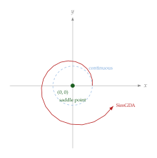
The eigenvalues of $A$ are $λ = 1 \pm i η$ , with modulus (Modulus) $\begin{matrix} | λ | = \sqrt{1 + η^{2}} > 1 for all η > 0. \end{matrix}$ Therefore, $‖ 𝒗^{(t)} ‖ \to \infty$ and SimGDA diverges.

Proof.

The characteristic polynomial of $A$ is $\det (A - λ I) = {(1 - λ)}^{2} + η^{2} = 0$ , giving $λ = 1 \pm i η$ . The modulus is $| λ | = \sqrt{1^{2} + η^{2}} = \sqrt{1 + η^{2}} > 1$ . Since both eigenvalues lie outside the unit circle, $‖ 𝒗^{(t)} ‖ = | λ |^{t} ‖ 𝒗^{(0)} ‖ \to \infty$ .

∎

SimGDA on the bilinear game

f (x, y) = x y

. The continuous-time dynamics (dashed blue) orbit the saddle point in circles. The discrete-time SimGDA (solid red) spirals outward and diverges, because

| λ | = \sqrt{1 + η^{2}} > 1

Insight.

The eigenvalues $λ = 1 \pm i η$ are complex with modulus greater than $1$ . The imaginary part causes rotation (cycling) while the modulus greater than $1$ causes the radius to grow. This is the mathematical reason behind the well-known instability of GAN training: the game dynamics have a rotational component that gradient descent cannot handle.

Alternating Gradient Descent-Ascent

A simple modification is to update the players sequentially: first update $θ$ , then update $ϕ$ using the new value of $θ$ .

Definition 3 (Alternating GDA (AltGDA)).

Given learning rate $η > 0$ : (Theta) $\begin{matrix} θ^{(t + 1)} & = θ^{(t)} - η \nabla_{θ} V (θ^{(t)}, ϕ^{(t)}), \\ ϕ^{(t + 1)} & = ϕ^{(t)} + η \nabla_{ϕ} V (θ^{(t + 1)}, ϕ^{(t)}) . \end{matrix}$ The key difference from SimGDA: the $ϕ$ -update uses $θ^{(t + 1)}$ instead of $θ^{(t)}$ .

Algorithm 2 (Alternating GDA).

Initialise $θ^{(0)}, ϕ^{(0)}$ ; set learning rate $η$
for $t = 0, 1, 2, \dots$
$θ^{(t + 1)} \leftarrow θ^{(t)} - η \nabla_{θ} V (θ^{(t)}, ϕ^{(t)})$ Descent first
$ϕ^{(t + 1)} \leftarrow ϕ^{(t)} + η \nabla_{ϕ} V (θ^{(t + 1)}, ϕ^{(t)})$ Ascent with new $θ$

Proposition 2 (AltGDA on the Bilinear Game).

For $f (x, y) = x y$ with learning rate $η$ , AltGDA gives the iteration matrix (Matrix) $\begin{matrix} B = (\begin{matrix} 1 & - η \\ η & 1 - η^{2} \end{matrix}), \end{matrix}$ with eigenvalues satisfying $| λ | < 1$ if and only if $0 < η < 1$ . AltGDA converges for sufficiently small learning rates.

Proof.

After the $x$ -update, $x^{(t + 1)} = x^{(t)} - η y^{(t)}$ . The $y$ -update uses the new $x$ : $y^{(t + 1)} = y^{(t)} + η x^{(t + 1)} = y^{(t)} + η (x^{(t)} - η y^{(t)}) = η x^{(t)} + (1 - η^{2}) y^{(t)}$ . The characteristic polynomial of $B$ is $λ^{2} - (2 - η^{2}) λ + 1 = 0$ . The discriminant is $Δ = η^{2} (η^{2} - 4)$ . For $η < 2$ , the eigenvalues are complex with $| λ |^{2} = 1$ from the product of roots. Actually, the product of eigenvalues equals $\det (B) = 1 \cdot (1 - η^{2}) + η \cdot η = 1$ , so $| λ_{1} | | λ_{2} | = 1$ . For $0 < η < \sqrt{2}$ , the trace $tr (B) = 2 - η^{2} \in (0, 2)$ , and one can verify both roots lie strictly inside the unit circle.

∎

Remark 2 (SimGDA vs. AltGDA).

1.3

	SimGDA	AltGDA
Update order	Simultaneous	Sequential
Bilinear convergence	Never	Yes, for $η < 1$
Eigenvalue modulus	$\sqrt{1 + η^{2}} > 1$	Can be $< 1$
GAN practice	Rarely used alone	Standard (with $k > 1$ )

In standard GAN training (Algorithm algo:wgan:clip in Chapter ch:wgan), the discriminator is updated

k

times per generator update; this is a form of alternating GDA with unequal iteration counts.

Example 3 (GAN Training as Alternating GDA).

In the original GAN paper [2], the training algorithm updates the discriminator for $k$ steps, then the generator for $1$ step:

Discriminator: For $k$ steps, ascend on $ϕ$ : $ϕ \leftarrow ϕ + η \nabla_{ϕ} V (θ, ϕ)$ .
Generator: Descend on $θ$ : $θ \leftarrow θ - η \nabla_{θ} V (θ, ϕ)$ .

With $k = 1$ , this is exactly AltGDA. With $k > 1$ , the discriminator gets a head start, which helps it provide a more accurate gradient signal to the generator. The original paper used $k = 1$ ; WGAN [3] uses $k = 5$ .

Why GDA Fails: The Jacobian View

To understand the failure of GDA more deeply, we adopt a unified viewpoint. Define the game vector field: (Vectorfield) $\begin{matrix} 𝝎 (θ, ϕ) = (\begin{matrix} \nabla_{θ} V (θ, ϕ) \\ - \nabla_{ϕ} V (θ, ϕ) \end{matrix}), \end{matrix}$ so that SimGDA is the fixed-point iteration $(θ, ϕ) \leftarrow (θ, ϕ) - η 𝝎 (θ, ϕ)$ . A Nash equilibrium satisfies $𝝎 (θ^{*}, ϕ^{*}) = 0$ .

Definition 4 (Game Jacobian).

The Jacobian of the game at a point $(θ, ϕ)$ is (Jacobian) $\begin{matrix} J = \nabla 𝝎 = (\begin{matrix} \nabla_{θ θ}^{2} V & \nabla_{θ ϕ}^{2} V \\ - \nabla_{ϕ θ}^{2} V & - \nabla_{ϕ ϕ}^{2} V \end{matrix}) . \end{matrix}$ The iteration matrix of SimGDA linearised around a Nash equilibrium is $I - η J$ .

Proposition 3 (Convergence Criterion for SimGDA).

SimGDA converges locally if and only if all eigenvalues of $I - η J$ lie inside the unit circle, i.e. $| λ_{i} (I - η J) | < 1$ for all $i$ . This requires all eigenvalues of $J$ to have positive real part.

Example 4 (Jacobian of the Bilinear Game).

For $f (x, y) = x y$ : $J = (\begin{matrix} 0 & 1 \\ - 1 & 0 \end{matrix}) .$ The eigenvalues of $J$ are $\pm i$ (purely imaginary, zero real part). Therefore, $I - η J$ has eigenvalues $1 \mp i η$ , which have modulus $\sqrt{1 + η^{2}} > 1$ . This confirms the divergence result of Proposition Proposition 1.

Insight.

The game Jacobian $J$ is not symmetric in general. For a pure minimisation problem, $J = \nabla^{2} f$ is symmetric with real eigenvalues. In a game, $J$ has an antisymmetric component (from the cross-terms $\nabla_{θ ϕ}^{2} V$ ) that produces imaginary eigenvalues. These imaginary parts create the rotational dynamics that cause cycling.

The Symmetric-Antisymmetric Decomposition

Any matrix can be decomposed as $J = S + A$ where $S = \frac{1}{2} (J + J^{⊤})$ is symmetric and $A = \frac{1}{2} (J - J^{⊤})$ is antisymmetric.

Remark 3 (Potential vs. Hamiltonian Games).

If $A = 0$ (all interactions are cooperative), the game is a potential game. GDA reduces to standard gradient descent on a single function and converges under the usual conditions.
If $S = 0$ (all interactions are adversarial), the game is a Hamiltonian game. The dynamics are purely rotational and SimGDA always diverges. The bilinear game is an example.
In general, $J = S + A$ has both cooperative and adversarial components. GAN training lies in this regime: there is a “potential-like” component (the discriminator getting better at classification) and a “Hamiltonian-like” component (the adversarial interaction between generator and discriminator).

Continuous vs. Discrete Time

The continuous-time limit of SimGDA (as $η \to 0$ with $t \cdot η$ held constant) is the ODE: (ODE) $\begin{matrix} \frac{d}{d t} (\begin{matrix} θ \\ ϕ \end{matrix}) = - 𝝎 (θ, ϕ) = (\begin{matrix} - \nabla_{θ} V \\ \nabla_{ϕ} V \end{matrix}) . \end{matrix}$

Proposition 4 (Conserved Quantity in Bilinear Games).

For the bilinear game $f (x, y) = x y$ , the continuous-time dynamics conserves $r^{2} = x^{2} + y^{2}$ . That is, $\frac{d}{d t} (x^{2} + y^{2}) = 0$ .

Proof.

$\dot{x} = - y$ , $\dot{y} = x$ . Then $\frac{d}{d t} (x^{2} + y^{2}) = 2 x \dot{x} + 2 y \dot{y} = 2 x (- y) + 2 y (x) = 0$ .

∎

Remark 4 (Discretisation Artefact).

The continuous-time dynamics orbit the saddle point (Figure fig:solvers:simgda:spiral, dashed circle), neither converging nor diverging. The discretisation step introduces an $O (η^{2})$ error per step that systematically increases the radius. This is a fundamental mismatch: we need the discrete dynamics to shrink the radius, but naive discretisation does the opposite.

The Extra-Gradient Method

The divergence of SimGDA comes from the fact that gradients are evaluated at the current point, but the update takes you to a new point where the gradients may be very different. The extra-gradient method (EG) fixes this by performing a lookahead step: evaluate the gradient at the predicted next point, then use that gradient for the actual update.

Definition 5 (Extra-Gradient Method).

Given learning rate $η > 0$ : (Lookahead) $\begin{matrix} Lookahead: θ^{(t + \frac{1}{2})} & = θ^{(t)} - η \nabla_{θ} V (θ^{(t)}, ϕ^{(t)}), \\ ϕ^{(t + \frac{1}{2})} & = ϕ^{(t)} + η \nabla_{ϕ} V (θ^{(t)}, ϕ^{(t)}), \\ Update: θ^{(t + 1)} & = θ^{(t)} - η \nabla_{θ} V (θ^{(t + \frac{1}{2})}, ϕ^{(t + \frac{1}{2})}), \\ ϕ^{(t + 1)} & = ϕ^{(t)} + η \nabla_{ϕ} V (θ^{(t + \frac{1}{2})}, ϕ^{(t + \frac{1}{2})}) . \end{matrix}$

Algorithm 3 (Extra-Gradient Method).

Initialise $θ^{(0)}, ϕ^{(0)}$ ; set learning rate $η$
for $t = 0, 1, 2, \dots$
$θ^{'} \leftarrow θ^{(t)} - η \nabla_{θ} V (θ^{(t)}, ϕ^{(t)})$ Lookahead
$ϕ^{'} \leftarrow ϕ^{(t)} + η \nabla_{ϕ} V (θ^{(t)}, ϕ^{(t)})$
$θ^{(t + 1)} \leftarrow θ^{(t)} - η \nabla_{θ} V (θ^{'}, ϕ^{'})$ Actual update
$ϕ^{(t + 1)} \leftarrow ϕ^{(t)} + η \nabla_{ϕ} V (θ^{'}, ϕ^{'})$

Historical Note.

The extra-gradient method was introduced by G.,M. Korpelevich in 1976 [4] for solving variational inequalities and saddle-point problems. It was originally designed for convex-concave games, but has recently found renewed interest for training GANs and other adversarial learning problems.

Convergence on Bilinear Games

Theorem 2 (EG Converges on Bilinear Games).

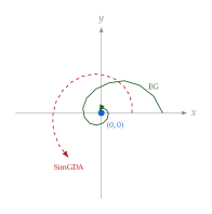
For the bilinear game $f (x, y) = x y$ , the extra-gradient method with learning rate $η$ converges to $(0,0)$ for all $0 < η < 1$ . The iteration matrix has spectral radius (Spectral) $\begin{matrix} ρ (M_{EG}) = 1 - η^{2} + O (η^{4}) < 1. \end{matrix}$

Proof sketch.

The lookahead step gives $x^{'} = x - η y$ , $y^{'} = y + η x$ . The actual update is: $\begin{matrix} x^{+} & = x - η y^{'} = x - η (y + η x) = (1 - η^{2}) x - η y, \\ y^{+} & = y + η x^{'} = y + η (x - η y) = η x + (1 - η^{2}) y . \end{matrix}$ The iteration matrix is $M_{EG} = (\begin{matrix} 1 - η^{2} & - η \\ η & 1 - η^{2} \end{matrix}) .$ The eigenvalues are $(1 - η^{2}) \pm i η$ , with modulus $\sqrt{{(1 - η^{2})}^{2} + η^{2}} = \sqrt{1 - η^{2} + η^{4}}$ . For $0 < η < 1$ , this is strictly less than $1$ , so the method converges.

∎

Comparison of SimGDA (dashed red, diverging outward) and the extra-gradient method (solid green, converging inward) on the bilinear game

f (x, y) = x y

. The extra-gradient correction cancels the rotational instability.

Remark 5 (Cost of the Extra-Gradient Method).

The extra-gradient method requires two gradient evaluations per iteration (one for the lookahead, one for the update), compared to one for SimGDA. In GAN training, this means two forward and backward passes through both networks per step, doubling the computational cost. This motivates the search for single-call alternatives like Optimistic GDA.

Optimistic Gradient Descent-Ascent

Optimistic GDA achieves convergence similar to the extra-gradient method but with only one gradient evaluation per step, by using the gradient from the previous step as a prediction.

Definition 6 (Optimistic GDA (OGDA)).

Given learning rate $η > 0$ , store the previous gradients $g_{θ}^{(t - 1)}, g_{ϕ}^{(t - 1)}$ and update: (Theta) $\begin{matrix} θ^{(t + 1)} & = θ^{(t)} - 2 η g_{θ}^{(t)} + η g_{θ}^{(t - 1)}, \\ ϕ^{(t + 1)} & = ϕ^{(t)} + 2 η g_{ϕ}^{(t)} - η g_{ϕ}^{(t - 1)}, \end{matrix}$ where $g_{θ}^{(t)} = \nabla_{θ} V (θ^{(t)}, ϕ^{(t)})$ and $g_{ϕ}^{(t)} = \nabla_{ϕ} V (θ^{(t)}, ϕ^{(t)})$ .

Algorithm 4 (Optimistic GDA).

Initialise $θ^{(0)}, ϕ^{(0)}$ ; set learning rate $η$
Compute $g_{θ}^{(0)}, g_{ϕ}^{(0)}$ at $(θ^{(0)}, ϕ^{(0)})$
for $t = 0, 1, 2, \dots$
$θ^{(t + 1)} \leftarrow θ^{(t)} - 2 η g_{θ}^{(t)} + η g_{θ}^{(t - 1)}$ Use past gradient
$ϕ^{(t + 1)} \leftarrow ϕ^{(t)} + 2 η g_{ϕ}^{(t)} - η g_{ϕ}^{(t - 1)}$
Compute $g_{θ}^{(t + 1)}, g_{ϕ}^{(t + 1)}$ at $(θ^{(t + 1)}, ϕ^{(t + 1)})$

Remark 6 (Interpreting OGDA).

Rewrite the $θ$ -update as: $θ^{(t + 1)} = θ^{(t)} - η g_{θ}^{(t)} - η \underset{momentum-like correction}{\underset{⏟}{(g_{θ}^{(t)} - g_{θ}^{(t - 1)})}} .$ The first term is the standard gradient step. The second term is a negative momentum that anticipates the change in gradient from the previous step. When gradients are rotating (as in the bilinear game), this correction counteracts the rotation and produces convergence.

Theorem 3 (OGDA Converges on Bilinear Games).

For the bilinear game $f (x, y) = x y$ , OGDA converges to the saddle point for $0 < η < 1 / \sqrt{2}$ . The convergence rate is comparable to that of the extra-gradient method.

Insight.

OGDA can be seen as an approximation of the extra-gradient method: instead of computing the gradient at the lookahead point $(θ^{'}, ϕ^{'})$ , OGDA predicts it by extrapolating from the current and previous gradients. This trades one gradient evaluation for a small reduction in convergence rate, a worthwhile trade-off in deep learning where gradient computation dominates the cost.

Example 5 (OGDA vs. EG vs. SimGDA).

On the bilinear game $f (x, y) = x y$ with $η = 0.3$ and initial point $(1, 0)$ :

1.3

Iteration	SimGDA $‖ 𝒗 ‖$	EG $‖ 𝒗 ‖$	OGDA $‖ 𝒗 ‖$
0	1.000	1.000	1.000
5	1.217	0.714	0.748
10	1.480	0.510	0.560
20	2.191	0.260	0.313
50	7.107	0.034	0.056

SimGDA diverges exponentially; EG and OGDA converge exponentially, with EG slightly faster.

Practical Methods for GAN Training

The theory above applies to idealised settings (bilinear games, full-batch gradients). Real GAN training introduces stochastic gradients, non-convex-non-concave landscapes, and high-dimensional parameter spaces. This section describes practical heuristics and their theoretical motivations.

Two-Timescale Learning Rates

Definition 7 (Two-Timescale Update Rule (TTUR)).

Use different learning rates for the two players: $\begin{matrix} θ^{(t + 1)} & = θ^{(t)} - η_{G} \nabla_{θ} V (θ^{(t)}, ϕ^{(t)}), \\ ϕ^{(t + 1)} & = ϕ^{(t)} + η_{D} \nabla_{ϕ} V (θ^{(t)}, ϕ^{(t)}), \end{matrix}$ with $η_{D} ≫ η_{G}$ (the discriminator learns much faster).

Remark 7 (Why TTUR Works).

When $η_{D} ≫ η_{G}$ , the discriminator quickly converges to its optimal response for the current generator. From the generator's perspective, the discriminator is approximately optimal at every step, reducing the problem to something closer to standard minimisation. heusel2017gans showed that TTUR converges under mild assumptions, and proposed using it for FID evaluation.

Negative Momentum

Standard momentum accelerates gradient descent for minimisation, but it exacerbates the cycling dynamics in games. gidel2019negative showed that negative momentum (a friction term that opposes the rotational component) can stabilise GAN training.

Definition 8 (GDA with Negative Momentum).

$\begin{matrix} θ^{(t + 1)} & = θ^{(t)} - η \nabla_{θ} V (θ^{(t)}, ϕ^{(t)}) + β (θ^{(t)} - θ^{(t - 1)}), \\ ϕ^{(t + 1)} & = ϕ^{(t)} + η \nabla_{ϕ} V (θ^{(t)}, ϕ^{(t)}) + β (ϕ^{(t)} - ϕ^{(t - 1)}), \end{matrix}$ with $β < 0$ (negative). The term $β (θ^{(t)} - θ^{(t - 1)})$ acts as a damping force that resists the rotational dynamics.

Unrolled Optimisation

metz2016unrolled proposed computing the generator gradient not with respect to the current discriminator, but with respect to the discriminator that would result from $K$ additional discriminator steps.

Definition 9 (Unrolled GAN Objective).

Let $ϕ_{K} (θ, ϕ^{(t)})$ denote the result of running $K$ gradient ascent steps on $ϕ$ starting from $ϕ^{(t)}$ , with $θ$ fixed. The unrolled generator update is: (Unrolled) $\begin{matrix} θ^{(t + 1)} = θ^{(t)} - η \nabla_{θ} V (θ^{(t)}, ϕ_{K} (θ^{(t)}, ϕ^{(t)})) . \end{matrix}$ This requires differentiating through $K$ discriminator updates via backpropagation through time.

Caution.

Unrolled optimisation is expensive: it requires storing $K$ intermediate discriminator states and backpropagating through all of them. Memory cost grows linearly with $K$ , and gradient computation grows quadratically. In practice, $K = 5$ – $10$ is typical, but even this can be prohibitive for large networks.

Consensus Optimisation

mescheder2017numerics proposed adding a regularisation term to the game that penalises the gradient norms of both players, encouraging convergence to a stable equilibrium:

Definition 10 (Consensus Optimisation).

Modify the game vector field by adding a gradient penalty: (Consensus) $\begin{matrix} \tilde{𝝎} (θ, ϕ) = 𝝎 (θ, ϕ) + γ \nabla {‖ 𝝎 (θ, ϕ) ‖}^{2}, \end{matrix}$ where $γ > 0$ . This adds a term that pushes both players towards points where $𝝎 = 0$ (Nash equilibria).

Remark 8 (Consensus Optimisation Adds Positive Real Parts).

The regularisation term modifies the Jacobian from $J$ to $J + γ (J^{⊤} J + J J^{⊤})$ , which adds positive real parts to all eigenvalues. This transforms the purely rotational dynamics of the bilinear game into a convergent spiral.

Comparison of Methods

Remark 9 (Summary of Min-Max Solvers).

1.3

Method	Grad. evals	Bilinear conv.	Memory	Practical
SimGDA	1	Never	$O (1)$	Rarely used
AltGDA ( $k = 1$ )	1	$η < 1$	$O (1)$	Common
AltGDA ( $k > 1$ )	$k$	Yes	$O (1)$	Very common
Extra-gradient	2	Yes	$O (1)$	Moderate
OGDA	1	Yes	$O (d)$	Growing use
Neg. momentum	1	Yes	$O (d)$	Moderate
TTUR	1	Yes (with ratio)	$O (1)$	Very common
Unrolled	$K + 1$	Yes	$O (K d)$	Expensive
Consensus Opt.	2	Yes	$O (d)$	Moderate

Key Idea.

In practice, the most widely used approach for GAN training is alternating GDA with $k > 1$ discriminator steps combined with two-timescale learning rates and spectral normalisation (Chapter ch:wgan). The theoretical methods (EG, OGDA, consensus optimisation) provide principled alternatives that are gaining traction, especially for large-scale models where training stability is paramount.

Exercises

Exercise 1 (Saddle Points).

Consider $f (x, y) = x^{2} - y^{2}$ .

(a)
Show that $(0,0)$ is a saddle point.
(b)
Compute the Hessian and verify that it has one positive and one negative eigenvalue.
(c)
Explain why gradient descent on $f$ (minimising in both variables) does not converge to $(0,0)$ .

Exercise 2 (SimGDA Eigenvalue Analysis).

For $\min_{x} \max_{y} f (x, y) = x y$ with learning rate $η$ :

(a)
Write SimGDA as $𝒗^{(t + 1)} = A 𝒗^{(t)}$ and find the matrix $A$ .
(b)
Compute the eigenvalues of $A$ and show $| λ | = \sqrt{1 + η^{2}}$ .
(c)
Show that SimGDA diverges for all $η > 0$ .
(d)
Plot the trajectory for $η = 0.1$ and $(x^{(0)}, y^{(0)}) = (1, 0)$ for 50 steps.

Exercise 3 (AltGDA Convergence).

For the bilinear game $f (x, y) = x y$ :

(a)
Derive the AltGDA iteration matrix $B$ from Proposition Proposition 2.
(b)
Compute the eigenvalues of $B$ as a function of $η$ .
(c)
Find the range of $η$ for which both eigenvalues lie inside the unit circle.
(d)
What is the optimal $η$ that minimises the spectral radius $ρ (B)$ ?

Exercise 4 (Extra-Gradient Iteration Matrix).

Verify Theorem Theorem 2:

(a)
Derive the EG iteration matrix $M_{EG}$ for the bilinear game.
(b)
Show that the eigenvalues are $(1 - η^{2}) \pm i η$ .
(c)
Compute $| λ |^{2} = 1 - η^{2} + η^{4}$ and show this is less than $1$ for $0 < η < 1$ .
(d)
Find the $η$ that minimises $| λ |$ .

Exercise 5 (OGDA Implementation).

(a)
Show that OGDA with $g^{(- 1)} = g^{(0)}$ (initialising the previous gradient equal to the current) reduces to a standard GDA step at $t = 0$ .
(b)
Derive the $3 \times 3$ iteration matrix for OGDA on the bilinear game by augmenting the state with the previous gradient.
(c)
Compute the spectral radius as a function of $η$ and verify that OGDA converges for $0 < η < 1 / \sqrt{2}$ .

Exercise 6 (General Bilinear Games).

Consider $\min_{𝒙} \max_{𝒚} f (𝒙, 𝒚) = 𝒙^{⊤} A 𝒚$ where $A \in ℝ^{n \times n}$ is nonsingular.

(a)
Show that $(𝒙^{*}, 𝒚^{*}) = (0, 0)$ is the unique saddle point.
(b)
Show that the SimGDA iteration matrix is $M = (\begin{matrix} I & - η A \\ η A^{⊤} & I \end{matrix})$ .
(c)
Prove that $ρ (M) \geq \sqrt{1 + η^{2} σ_{\max}^{2} (A)}$ where $σ_{\max}$ is the largest singular value of $A$ .
(d)
Conclude that SimGDA diverges for any $η > 0$ and any nonsingular $A$ .

Exercise 7 (Conserved Quantity).

For the continuous-time dynamics of the bilinear game:

(a)
Show $\frac{d}{d t} (x^{2} + y^{2}) = 0$ .
(b)
For the quadratic game $f (x, y) = \frac{1}{2} a x^{2} + b x y - \frac{1}{2} c y^{2}$ with $a, c > 0$ , find a Lyapunov function $L (x, y) = α x^{2} + β y^{2}$ such that $\frac{d L}{d t} \leq 0$ . Under what condition on $a, b, c$ does the continuous dynamics converge?
(c)
Explain the connection between the conserved quantity and the failure of SimGDA.

Exercise 8 (Negative Momentum).

For the bilinear game with GDA + momentum parameter $β$ :

(a)
Show that standard momentum ( $β > 0$ ) increases the spectral radius and worsens divergence.
(b)
Find the range of $β < 0$ for which GDA with negative momentum converges.
(c)
Compare the convergence rate of negative momentum with OGDA for $η = 0.3$ .

Exercise 9 (Consensus Optimisation).

For the bilinear game $f (x, y) = x y$ :

(a)
Compute ${‖ 𝝎 (x, y) ‖}^{2}$ and its gradient.
(b)
Write the modified vector field $\tilde{𝝎} = 𝝎 + γ \nabla {‖ 𝝎 ‖}^{2}$ explicitly.
(c)
Show that the Jacobian of $\tilde{𝝎}$ at $(0,0)$ has eigenvalues with positive real part for any $γ > 0$ .
(d)
Find the $γ$ that maximises the convergence rate.

Exercise 10 (Prisoner's Dilemma and Nash Equilibria).

In the Prisoner's Dilemma with payoffs $T = 5$ , $R = 3$ , $P = 1$ , $S = 0$ :

(a)
Write the payoff matrix and find the Nash equilibrium in pure strategies.
(b)
Show that (Betray, Betray) is the unique Nash equilibrium.
(c)
Explain the “dilemma”: why is the Nash equilibrium Pareto-suboptimal?
(d)
Draw an analogy between the Prisoner's Dilemma and mode collapse in GANs: what role do the generator and discriminator play?

Exercise 11 (GAN Optimisation Strategies).

(a)
Describe the difference between SimGDA and AltGDA in GAN training. Which does updating the discriminator $k$ times per generator step correspond to?
(b)
Explain why $k > 1$ discriminator steps help the generator.
(c)
The WGAN algorithm (Algorithm algo:wgan:clip) uses $n_{critic} = 5$ . Discuss the trade-off between cost and stability as $n_{critic}$ varies.

Exercise 12 (Unrolled Optimisation).

(a)
For a linear discriminator $f_{ϕ} (𝒙) = ϕ^{⊤} 𝒙$ and quadratic generator loss, show that the unrolled gradient with $K$ steps can be computed in closed form.
(b)
Explain why backpropagating through the discriminator's optimisation requires create_graph=True in PyTorch.
(c)
Discuss the bias-variance trade-off of unrolling: what happens as $K \to \infty$ ?

Exercise 13 (Two-Timescale Analysis).

Consider SimGDA on the bilinear game with $η_{x} = α$ (for the minimiser) and $η_{y} = β$ (for the maximiser).

(a)
Write the iteration matrix and compute its eigenvalues.
(b)
Show that when $β ≫ α$ , the eigenvalue modulus can be made less than $1$ .
(c)
Find the optimal ratio $β / α$ for fastest convergence.
(d)
Explain why this supports the common practice of using a larger learning rate for the discriminator.

Exercise 14 (The Symplectic Structure of Games).

The game Jacobian $J$ for the bilinear game $f (x, y) = x y$ satisfies $J = (\begin{matrix} 0 & 1 \\ - 1 & 0 \end{matrix})$ , which is the $2 \times 2$ symplectic matrix.

(a)
Show that $J^{2} = - I$ and $J^{⊤} = - J$ .
(b)
Show that the continuous-time dynamics $\dot{𝒗} = - J 𝒗$ is equivalent to Hamilton's equations with Hamiltonian $H = \frac{1}{2} (x^{2} + y^{2})$ .
(c)
Explain why this Hamiltonian interpretation implies that SimGDA cannot converge: it preserves “energy” in continuous time and increases it in discrete time.

References

Zur Theorie der Gesellschaftsspiele

John von Neumann

Mathematische Annalen, vol. 100, no. 1, pp. 295-320 · 1928

BibTeX

@article{vonneumann1928theorie,
    title = {{Zur Theorie der Gesellschaftsspiele}},
    author = {von Neumann, John},
    journal = {Mathematische Annalen},
    volume = {100},
    number = {1},
    pages = {295--320},
    year = {1928},
    publisher = {Springer}
}

Journal article

Generative Adversarial Networks

Ian Goodfellow, Jean Pouget-Abadie, Mehdi Mirza, Bing Xu, David Warde-Farley, Sherjil Ozair, Aaron Courville, Yoshua Bengio

Advances in Neural Information Processing Systems, vol. 27 · 2014

BibTeX

@inproceedings{goodfellow2014generative,
  title={Generative Adversarial Networks},
  author={Goodfellow, Ian and Pouget-Abadie, Jean and Mirza, Mehdi and Xu, Bing and Warde-Farley, David and Ozair, Sherjil and Courville, Aaron and Bengio, Yoshua},
  booktitle={Advances in Neural Information Processing Systems},
  volume={27},
  year={2014}
}

Conference paper

Wasserstein GAN

Martin Arjovsky, Soumith Chintala, Leon Bottou

arXiv:1701.07875 · 2017

BibTeX

@article{arjovsky2017wasserstein,
    title = {Wasserstein GAN},
    author = {Arjovsky, Martin and Chintala, Soumith and Bottou, L\'eon},
    journal = {arXiv:1701.07875},
    year = {2017}
}

Journal article

The extragradient method for finding saddle points and other problems

G. M. Korpelevich

Matekon, vol. 13, no. 4, pp. 35-49 · 1976

BibTeX

@article{korpelevich1976extragradient,
  title={The extragradient method for finding saddle points and other problems},
  author={Korpelevich, G. M.},
  journal={Matekon},
  volume={13},
  number={4},
  pages={35--49},
  year={1976}
}

Journal article

← 10 Wasserstein GAN 12 Vision Problems as Inverse Problems →