12 Vision Problems as Inverse Problems

Vision Meets Generation

The previous chapters developed the theory of generative models, including GANs, Wasserstein distances, and min-max optimisation. In this chapter, we show that many classical computer vision problems are inverse problems that can be solved by learned generative priors. This provides the mathematical bridge between the theory of Parts I–III and the applications in the next chapter.

Key Idea.

If you can generate realistic images, you can also restore them. A generative model that has learned the distribution of natural images encodes a powerful prior $p (𝒙)$ over the image space. Combining this prior with a physical forward model $𝒚 = 𝒜 (𝒙) + 𝒏$ turns every inverse problem (denoising, super-resolution, inpainting, style transfer) into a posterior inference problem.

The chapter is organised as follows. We first introduce the general framework of inverse problems in imaging (Section Inverse Problems in Imaging). We then study five fundamental vision tasks, namely denoising (Section Image Denoising), super-resolution (Section Super-Resolution), inpainting (Section Image Inpainting), style transfer (Section Style Transfer and Texture Synthesis), and image-to-image translation (Section Image-to-Image Translation), formulating each as an inverse problem and tracing the path from classical solutions to generative approaches. We close with a unifying perspective on the generative prior (Section The Generative Prior).

Inverse Problems in Imaging

Definition 1 (Forward Model).

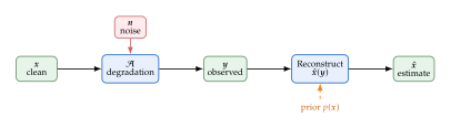
An imaging forward model describes the physical process that produces an observation $𝒚$ from a clean image $𝒙$ : (Forward) $\begin{matrix} 𝒚 = 𝒜 (𝒙) + 𝒏, \end{matrix}$ where $𝒜 : ℝ^{n} \to ℝ^{m}$ is a (possibly nonlinear) degradation operator and $𝒏$ is observation noise.

Example 1 (Forward Models for Common Tasks).

1.4

Task	Operator $𝒜$	Observation $𝒚$
Denoising	Identity: $𝒜 = I$	$𝒚 = 𝒙 + 𝒏$
Super-resolution	Downsample: $𝒜 = D \in ℝ^{m \times n}, m ≪ n$	$𝒚 = D 𝒙 + 𝒏$
Inpainting	Mask: $𝒜 = diag (𝒎), m_{i} \in {0,1}$	$𝒚 = 𝒎 ⊙ 𝒙 + 𝒏$
Deblurring	Convolution: $𝒜 (𝒙) = 𝒌 * 𝒙$	$𝒚 = 𝒌 * 𝒙 + 𝒏$
Compressed sensing	Random projection: $𝒜 = Φ \in ℝ^{m \times n}$	$𝒚 = Φ 𝒙 + 𝒏$

The inverse problem pipeline. A clean image

𝒙

is degraded by operator

𝒜

and corrupted by noise

𝒏

to produce observation

𝒚

. Reconstruction requires inverting this process, which is typically ill-posed and needs a prior

p (𝒙)

to regularise the solution.

Ill-Posedness

Definition 2 (Well-Posed Problem (Hadamard, 1902)).

A problem is well-posed in the sense of Hadamard if:

A solution exists.
The solution is unique.
The solution depends continuously on the data.

A problem that violates any of these conditions is ill-posed.

Remark 1 (Most Vision Problems Are Ill-Posed).

Super-resolution: The downsampling operator $D$ maps many high-resolution images to the same low-resolution observation, so the solution is not unique.
Inpainting: The missing pixels can be filled in infinitely many ways, so again not unique.
Denoising: The inverse of the identity is the identity (trivially well-posed), but the noise makes the problem discontinuous: small changes in $𝒚$ can produce large changes in $\hat{𝒙}$ without regularisation.

Bayesian Formulation

The Bayesian approach resolves ill-posedness by introducing a prior $p (𝒙)$ over images:

Definition 3 (MAP Estimation).

The maximum a posteriori (MAP) estimate is (MAP) $\begin{matrix} {\hat{𝒙}}_{MAP} = {arg max}_{𝒙} p (𝒙 | 𝒚) = {arg max}_{𝒙} [\log p (𝒚 | 𝒙) + \log p (𝒙)], \end{matrix}$ where $p (𝒚 | 𝒙)$ is the likelihood (determined by the forward model and noise distribution) and $p (𝒙)$ is the prior.

Example 2 (MAP for Gaussian Denoising).

For $𝒚 = 𝒙 + 𝒏$ with $𝒏 \sim 𝒩 (0, σ^{2} I)$ : $\log p (𝒚 | 𝒙) = - \frac{1}{2 σ^{2}} {‖ 𝒚 - 𝒙 ‖}^{2} + const.$ The MAP estimate becomes: (Gaussian) $\begin{matrix} {\hat{𝒙}}_{MAP} = {arg min}_{𝒙} [\frac{1}{2 σ^{2}} {‖ 𝒚 - 𝒙 ‖}^{2} - \log p (𝒙)] . \end{matrix}$ The first term pulls $\hat{𝒙}$ towards the observation; the second term pulls it towards “natural-looking” images. The balance between the two is controlled by the noise level $σ$ .

Insight.

Every choice of prior $p (𝒙)$ yields a different restoration algorithm:

$p (𝒙) \propto \exp (- λ {‖ \nabla 𝒙 ‖}_{1})$ $\Rightarrow$ total-variation denoising
$p (𝒙) \propto \exp (- λ {‖ W 𝒙 ‖}_{1})$ $\Rightarrow$ wavelet shrinkage
$p (𝒙) = p_{θ} (𝒙)$ from a GAN/VAE/diffusion model $\Rightarrow$ generative prior

The evolution from hand-crafted priors to learned generative priors is the central story of modern computational imaging.

Image Denoising

Denoising is the simplest inverse problem: the forward model is the identity, and the task is to undo the effect of additive noise.

Definition 4 (Image Denoising Problem).

Given a noisy observation (Denoise) $\begin{matrix} 𝒚 = 𝒙 + 𝒏, 𝒏 \sim 𝒩 (0, σ^{2} I), \end{matrix}$ estimate the clean image $𝒙$ .

Classical Methods

Remark 2 (A Hierarchy of Denoising Methods).

Gaussian filter. Replace each pixel by a weighted average of its neighbours: $\hat{𝒙} = G_{σ} * 𝒚$ . Simple but blurs edges.
Bilateral filter. Weight neighbours by both spatial distance and intensity similarity, preserving edges while smoothing flat regions.
Non-local means (NLM). Average pixels whose patches (not just individual pixels) are similar, exploiting the self-similarity of natural images [1].
BM3D. Group similar patches into 3D stacks, apply a 3D transform (e.g. wavelet), threshold, and invert. State-of-the-art among non-learned methods [2].
Deep denoisers. Train a neural network $f_{θ}$ to minimise $𝔼 [{‖ f_{θ} (𝒚) - 𝒙 ‖}^{2}]$ over a dataset of (noisy, clean) pairs. The DnCNN architecture [3] and its successors consistently outperform BM3D.

Historical Note.

The connection between denoising and generative modelling runs deep. Vincent et al. (2008, 2010) showed that training an autoencoder to denoise is equivalent to learning the score function $\nabla_{𝒙} \log p (𝒙)$ of the data distribution, the very quantity that score-based diffusion models (Part VI of this book) use to generate images. In this sense, denoising is not just an application of generative models; it is their foundation.

The MMSE Estimator

Theorem 1 (Optimal Denoiser).

The estimator that minimises the mean squared error $𝔼 [{‖ \hat{𝒙} - 𝒙 ‖}^{2}]$ is the posterior mean: (MMSE) $\begin{matrix} {\hat{𝒙}}_{MMSE} (𝒚) = 𝔼 [𝒙 | 𝒚] = \int 𝒙 p (𝒙 | 𝒚) d 𝒙 . \end{matrix}$

Proof.

For any estimator $\hat{𝒙} (𝒚)$ : $\begin{matrix} 𝔼 [{‖ \hat{𝒙} - 𝒙 ‖}^{2}] & = 𝔼 [{‖ \hat{𝒙} - 𝔼 [𝒙 | 𝒚] + 𝔼 [𝒙 | 𝒚] - 𝒙 ‖}^{2}] \\ = 𝔼 [{‖ \hat{𝒙} - 𝔼 [𝒙 | 𝒚] ‖}^{2}] + 𝔼 [{‖ 𝔼 [𝒙 | 𝒚] - 𝒙 ‖}^{2}], \end{matrix}$ since the cross-term vanishes by the tower property. The first term is minimised (to zero) when $\hat{𝒙} = 𝔼 [𝒙 | 𝒚]$ .

∎

Caution.

The MMSE estimator $𝔼 [𝒙 | 𝒚]$ averages over all plausible clean images, which produces blurry results when the posterior is multimodal. For example, if a noisy image could be either a cat or a dog, the MMSE estimate is a blurry blend of the two. This is why perceptual quality metrics (LPIPS, FID) and MAP/sampling-based approaches are often preferred in practice.

Super-Resolution

Definition 5 (Single-Image Super-Resolution).

Given a low-resolution observation (SR) $\begin{matrix} 𝒚 = D 𝒙 + 𝒏, \end{matrix}$ where $D \in ℝ^{m \times n}$ with $m ≪ n$ is a downsampling operator (e.g. bicubic downsampling by factor $s$ ), estimate the high-resolution image $𝒙 \in ℝ^{n}$ .

Remark 3 (Ill-Posedness of Super-Resolution).

For $s$ -fold super-resolution, each low-resolution pixel corresponds to $s^{2}$ high-resolution pixels. The system $𝒚 = D 𝒙$ is massively underdetermined: there are $s^{2}$ times more unknowns than equations. Without a prior, there are infinitely many valid high-resolution images consistent with the observation.

Example 3 (The PSNR–Perceptual Quality Trade-Off).

Consider $4 \times$ super-resolution of a face image:

Bicubic interpolation: Smooth, blurry output. High PSNR but low perceptual quality.
MSE-trained CNN: Sharper than bicubic, but still blurry on fine details (hair, skin texture). Maximises PSNR.
GAN-based (SRGAN): Generates sharp, realistic textures. Lower PSNR than the CNN, but much higher perceptual quality.

This paradox arises because PSNR measures pixel-wise accuracy, while perceptual quality depends on whether the image “looks real.” The MMSE solution maximises PSNR but averages over the posterior, producing blur. A GAN samples from the posterior, producing sharp but potentially inaccurate details.

Insight.

The PSNR–perceptual quality trade-off is a distortion–perception trade-off, and it is worth being precise about which quantity does the work, because the intuitive reading is backwards. Conditioned on $𝒚$ , both candidate estimators are unbiased: $𝔼 [{\hat{𝒙}}_{MMSE} | 𝒚] = 𝔼 [𝒙 | 𝒚]$ , and a posterior sample also has conditional mean $𝔼 [𝒙 | 𝒚]$ . They differ in variance, and it is the posterior mean that has none: given $𝒚$ it is a single deterministic image, and that absence of variability is exactly what blur is. Averaging away the variation across plausible images is what makes the result look unreal.

Writing $Σ = 𝖵ar (𝒙 | 𝒚)$ for the posterior variance, the two estimators cost $𝔼 [{‖ 𝔼 [𝒙 | 𝒚] - 𝒙 ‖}^{2} | 𝒚] = tr Σ, 𝔼 [{‖ 𝒙^{'} - 𝒙 ‖}^{2} | 𝒚] = 2 tr Σ for 𝒙^{'} \sim p (𝒙 | 𝒚),$ since an independent sample contributes its own $tr Σ$ on top of the target's. A posterior sample therefore pays exactly twice the squared error of the posterior mean, while carrying the full posterior variance that makes it look like a real image. Realism is bought with distortion, and any pixel-wise metric such as PSNR will prefer the blur every time.

Classical to Learned Super-Resolution

Remark 4 (Evolution of Super-Resolution).

Interpolation (nearest, bilinear, bicubic): Simple, fast, but does not add any new information.
Sparse coding [4]: Learn a dictionary of high-resolution patches and reconstruct using sparse coefficients.
SRCNN [5]: First deep learning approach, a 3-layer CNN that maps low-resolution to high-resolution. Set a new state of the art in 2014.
SRGAN [6]: Added a GAN loss and a perceptual loss (VGG features) to produce photorealistic super-resolution. We study this in detail in the next chapter.

Image Inpainting

Definition 6 (Image Inpainting Problem).

Given an image $𝒙$ and a binary mask $𝒎 \in {0,1}^{n}$ (where $m_{i} = 0$ indicates a missing pixel), the observation is (Inpaint) $\begin{matrix} 𝒚 = 𝒎 ⊙ 𝒙, \end{matrix}$ where $⊙$ denotes element-wise multiplication. The task is to estimate the original image $𝒙$ from the observed pixels $𝒚$ and the mask $𝒎$ .

Remark 5 (Degrees of Freedom in Inpainting).

If $k$ pixels are missing (i.e. $\sum_{i} (1 - m_{i}) = k$ ), then the problem has $k$ free parameters and $n - k$ constraints. For a small scratch ( $k \approx 100$ ), the problem is mildly underdetermined; for a large hole ( $k \approx n / 2$ ), it is severely underdetermined and requires strong priors.

Classical Approaches

Example 4 (Three Classical Inpainting Strategies).

Diffusion-based [7]: Propagate information from known pixels into the missing region using a PDE that mimics heat diffusion: $\partial_{t} 𝒙 = Δ 𝒙$ in the missing region, with Dirichlet boundary conditions from the known pixels. Good for thin scratches, poor for large holes.
Patch-based [9]: Search the known region for patches similar to the boundary of the hole, and copy them in. The “image quilting” approach of Efros and Freeman [8] is a related technique. Good for textured regions, poor for structured content.
Generative: Use a generative model (GAN, VAE, diffusion) to sample plausible completions conditioned on the known pixels. Can hallucinate coherent structure (faces, objects) in large missing regions.

Key Idea.

Inpainting is perhaps the clearest demonstration of why generative models matter for vision: filling a large hole in an image requires imagining what could be there, which is exactly what a generative model is trained to do.

Style Transfer and Texture Synthesis

Style transfer and texture synthesis ask a different kind of question: not “what was the original image?” but “what would this image look like in a different style?”

Texture Synthesis

Definition 7 (Texture Synthesis Problem).

Given a small texture exemplar $𝒙_{ex} \in ℝ^{n_{1}}$ , generate a larger image $\hat{𝒙} \in ℝ^{n_{2}}$ ( $n_{2} ≫ n_{1}$ ) that is perceptually indistinguishable from the exemplar; it should appear to be a different sample from the same texture distribution.

Remark 6 (Texture Synthesis Methods).

Pixel-based [10]: Synthesise one pixel at a time by matching local neighbourhoods. Slow but handles stochastic textures well.
Patch-based (Image Quilting) [8]: Stitch overlapping patches together with minimum-error boundary cuts. Fast and effective for many textures.
Parametric (Gram matrix) [11]: Match the Gram matrices of CNN feature maps between the exemplar and the synthesised image. This is the foundation of neural style transfer.

Neural Style Transfer

The breakthrough of Gatys et al. [13] was to show that the “style” of an image can be captured by the correlations between features in a pretrained CNN.

Definition 8 (Gram Matrix).

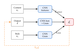
Let $F^{ℓ} \in ℝ^{C_{ℓ} \times H_{ℓ} W_{ℓ}}$ be the feature map of layer $ℓ$ of a pretrained CNN (e.g. VGG-19), where $C_{ℓ}$ is the number of channels and $H_{ℓ} W_{ℓ}$ is the spatial size. The Gram matrix is (GRAM) $\begin{matrix} G^{ℓ} = \frac{1}{C_{ℓ} H_{ℓ} W_{ℓ}} F^{ℓ} {(F^{ℓ})}^{⊤} \in ℝ^{C_{ℓ} \times C_{ℓ}} . \end{matrix}$ Entry $G_{i j}^{ℓ}$ measures the correlation between feature channels $i$ and $j$ at layer $ℓ$ .

Definition 9 (Neural Style Transfer Loss).

Given a content image $𝒙_{c}$ and a style image $𝒙_{s}$ , generate an output $\hat{𝒙}$ that minimises (NST) $\begin{matrix} ℒ (\hat{𝒙}) = \underset{content loss ℒ_{content}}{\underset{⏟}{\sum_{ℓ} α_{ℓ} {‖ F^{ℓ} (\hat{𝒙}) - F^{ℓ} (𝒙_{c}) ‖}_{F}^{2}}} + \underset{style loss ℒ_{style}}{\underset{⏟}{\sum_{ℓ} β_{ℓ} {‖ G^{ℓ} (\hat{𝒙}) - G^{ℓ} (𝒙_{s}) ‖}_{F}^{2}}}, \end{matrix}$ where $α_{ℓ}, β_{ℓ}$ control the balance between content fidelity and style fidelity.

Neural style transfer optimises the output image

\hat{𝒙}

to match the content features of

𝒙_{c}

and the Gram-matrix style statistics of

𝒙_{s}

. The gradient flows back to the image pixels.

Historical Note.

The idea of “image analogies” ( $A$ is to $B$ as $C$ is to $D$ ) was introduced by Hertzmann et al. [12] in 2001. It used patch-based nearest-neighbour search to transfer the transformation between an exemplar pair $(A, B)$ to a new input $C$ . Fifteen years later, Gatys et al. [13] showed that a pretrained CNN provides a far more powerful feature space for style representation. This opened the door to real-time style transfer using feed-forward networks [14], and eventually to GAN-based methods like pix2pix (Chapter 13).

Example 5 (Reading the Style Transfer Loss).

Content loss matches spatial feature maps: it preserves the “what” and “where” of the content image (objects, edges, layout).
Style loss matches feature correlations: it captures the “how” of the style image (brushstrokes, colour palette, textures), stripped of spatial arrangement.
Increasing $β_{ℓ} / α_{ℓ}$ makes the output more “stylised” (more like $𝒙_{s}$ ); decreasing it makes it more “photographic” (more like $𝒙_{c}$ ).

Image-to-Image Translation

Many vision tasks can be viewed as translating an image from one domain to another: edges $\to$ photos, day $\to$ night, labels $\to$ facades, horses $\to$ zebras.

Definition 10 (Image-to-Image Translation).

Given paired training data ${(𝒙_{i}^{A}, 𝒙_{i}^{B})}_{i = 1}^{N}$ from two domains $A$ and $B$ , learn a mapping $G : A \to B$ such that $G (𝒙^{A})$ is indistinguishable from real samples in domain $B$ .

Remark 7 (Paired vs. Unpaired Translation).

Paired: Each input has a corresponding output (e.g. satellite image $\leftrightarrow$ map). The loss can include a pixel-wise $L_{1}$ term. Example: pix2pix [15].
Unpaired: We have images from domain $A$ and images from domain $B$ , but no correspondences. The loss relies on a cycle-consistency constraint. Example: CycleGAN [16].

Both approaches are studied in detail in the next chapter.

Example 6 (Image-to-Image Tasks as Translation).

1.3

Task	Domain $A$	Domain $B$
Semantic segmentation	Photo	Label map
Colourisation	Grayscale	Colour
Edge-to-photo	Edge map	Photo
Day-to-night	Daytime photo	Nighttime photo
Style transfer	Photo	Painting
Super-resolution	Low-res	High-res
Inpainting	Masked image	Complete image

Many of the inverse problems we studied earlier in this chapter are special cases of image-to-image translation!

Key Idea.

Image-to-image translation is the Swiss army knife of generative vision. By casting each task as a translation between two domains, a single framework (conditional GAN + perceptual loss) can handle denoising, super-resolution, colourisation, segmentation, style transfer, and more. The next chapter develops this idea in detail.

The Generative Prior

We can now see the common thread running through all the problems in this chapter: each one is an inverse problem that requires a prior over natural images.

Definition 11 (Generative Prior).

A generative prior is a prior $p (𝒙)$ over images that is implicitly or explicitly defined by a generative model (GAN, VAE, normalising flow, or diffusion model). Given an inverse problem $𝒚 = 𝒜 (𝒙) + 𝒏$ , the generative prior enables:

MAP estimation: $\hat{𝒙} = {arg min}_{𝒙} [{‖ 𝒚 - 𝒜 (𝒙) ‖}^{2} + λ R (𝒙)]$ where $R (𝒙) = - \log p (𝒙)$ .
Posterior sampling: $\hat{𝒙} \sim p (𝒙 | 𝒚)$ via MCMC or diffusion-based methods.
Projection: $\hat{𝒙} = G_{θ} (\hat{𝒛})$ where $\hat{𝒛} = {arg min}_{𝒛} {‖ 𝒚 - 𝒜 (G_{θ} (𝒛)) ‖}^{2}$ projects the observation onto the range of the generator.

Remark 8 (From Hand-Crafted to Learned Priors).

1.3

Era	Prior $p (𝒙)$	Examples
1990s	Smoothness (Tikhonov)	$R (𝒙) = {‖ \nabla 𝒙 ‖}^{2}$
2000s	Sparsity (compressed sensing)	$R (𝒙) = {‖ W 𝒙 ‖}_{1}$
2010s	Patch-based (BM3D, NLM)	Self-similarity
2014+	Deep generative (GAN, VAE)	$p_{θ} (𝒙)$ from data
2020+	Diffusion models	$\nabla_{𝒙} \log p_{t} (𝒙)$

Each generation of priors better captures the statistics of natural images, leading to better inverse-problem solutions.

Example 7 (GAN Projection for Inpainting).

Suppose we have a pretrained GAN generator $G_{θ} : ℝ^{k} \to ℝ^{n}$ . To inpaint a masked image $𝒚 = 𝒎 ⊙ 𝒙$ :

Optimise over the latent space: $\hat{𝒛} = {arg min}_{𝒛} {‖ 𝒎 ⊙ G_{θ} (𝒛) - 𝒚 ‖}^{2}$ .
The reconstruction is $\hat{𝒙} = G_{θ} (\hat{𝒛})$ .

Because $G_{θ}$ can only produce images in the learned manifold of natural images, the missing pixels are automatically filled with plausible content. This technique requires no task-specific training, only a pretrained generator.

Insight.

The generative prior provides a universal regulariser: the same GAN or diffusion model can be applied to denoising, super-resolution, inpainting, colourisation, and compressed sensing, simply by changing the forward model $𝒜$ while keeping $p (𝒙)$ fixed. This “plug-and-play” approach is one of the most powerful ideas in modern computational imaging.

Exercises

Exercise 1 (MAP for Gaussian Denoising).

Consider $𝒚 = 𝒙 + 𝒏$ with $𝒏 \sim 𝒩 (0, σ^{2} I)$ and a Gaussian prior $𝒙 \sim 𝒩 (0, Σ)$ .

(a)
Show that the MAP estimate is $\hat{𝒙} = Σ {(Σ + σ^{2} I)}^{- 1} 𝒚$ .
(b)
Verify that as $σ \to 0$ , $\hat{𝒙} \to 𝒚$ (no denoising needed).
(c)
Verify that as $σ \to \infty$ , $\hat{𝒙} \to 0$ (rely entirely on the prior).
(d)
Compute the MMSE estimator and show it coincides with the MAP for this Gaussian case.

Exercise 2 (Total-Variation Denoising).

The total-variation (TV) prior on a 1D signal $𝒙 \in ℝ^{n}$ is $R (𝒙) = \sum_{i = 1}^{n - 1} | x_{i + 1} - x_{i} |$ .

(a)
Write the TV-regularised denoising problem as a minimisation.
(b)
Show that the TV prior encourages piecewise-constant signals.
(c)
Explain why TV denoising preserves edges but produces “staircase” artefacts in smooth regions.
(d)
Propose a modification to handle smooth regions better.

Exercise 3 (Super-Resolution as a Linear Inverse Problem).

For $2 \times$ super-resolution of a $4 \times 4$ image to $8 \times 8$ :

(a)
Write the downsampling operator $D$ as a matrix.
(b)
What is the rank of $D$ ? How many dimensions of $𝒙$ are unobservable?
(c)
Show that without a prior, the least-squares solution $D^{⊤} {(D D^{⊤})}^{- 1} 𝒚$ is equivalent to nearest-neighbour upsampling.
(d)
Explain how a prior changes this solution.

Exercise 4 (Inpainting with a Known Image Model).

Suppose $𝒙 \sim 𝒩 (𝝁, Σ)$ and we observe $𝒚 = 𝒎 ⊙ 𝒙$ (noise-free, masked). Partition $𝒙$ into observed components $𝒙_{o}$ and missing components $𝒙_{m}$ .

(a)
Show that $p (𝒙_{m} | 𝒙_{o})$ is Gaussian and compute its mean and covariance using the Schur complement.
(b)
What happens when the prior covariance $Σ$ is diagonal? Why is this a poor model for natural images?
(c)
Explain qualitatively how a GAN prior improves upon the Gaussian prior for this task.

Exercise 5 (Gram Matrix Properties).

(a)
Show that the Gram matrix $G = F F^{⊤}$ is symmetric and positive semidefinite.
(b)
Show that $G_{i j} = ⟨ 𝒇_{i}, 𝒇_{j} ⟩$ where $𝒇_{i}$ is the $i$ -th row of $F$ (the activation of channel $i$ across all spatial locations).
(c)
Explain why matching Gram matrices captures “style” (correlations between features) rather than “content” (spatial arrangement).
(d)
If the feature map has $C$ channels and spatial size $H \times W$ , what is the dimensionality of the Gram matrix? Is this efficient for large feature maps?

Exercise 6 (Content vs. Style Loss).

Consider a neural style transfer setup with a single content layer $ℓ_{c}$ and a single style layer $ℓ_{s}$ .

(a)
If we set $α = 1, β = 0$ , what does the output look like? What about $α = 0, β = 1$ ?
(b)
Explain why using deeper layers for the content loss preserves semantic structure but not fine details.
(c)
Explain why using earlier layers for the style loss captures low-level textures while later layers capture higher-level style elements.

Exercise 7 (Perceptual Loss vs. Pixel Loss).

Consider training a super-resolution network $f_{θ}$ with two possible losses: $\begin{matrix} ℒ_{pixel} & = 𝔼 [{‖ f_{θ} (𝒚) - 𝒙 ‖}^{2}], \\ ℒ_{perceptual} & = 𝔼 [{‖ Φ (f_{θ} (𝒚)) - Φ (𝒙) ‖}^{2}], \end{matrix}$ where $Φ$ extracts features from a pretrained VGG network.

(a)
Explain why minimising $ℒ_{pixel}$ leads to blurry outputs.
(b)
Why does $ℒ_{perceptual}$ produce sharper results?
(c)
Design a combined loss for super-resolution that includes pixel, perceptual, and adversarial components. Explain the role of each term.

Exercise 8 (GAN Projection).

A pretrained GAN maps $𝒛 \in ℝ^{100}$ to images $G (𝒛) \in ℝ^{64 \times 64 \times 3}$ .

(a)
For denoising via GAN projection, $\hat{𝒛} = {arg min}_{𝒛} {‖ G (𝒛) - 𝒚 ‖}^{2}$ , explain why the output is guaranteed to be a “natural-looking” image.
(b)
What are the limitations of this approach? (Hint: consider the expressiveness of the generator.)
(c)
How would you modify the approach to handle super-resolution? Inpainting?

Exercise 9 (Paired vs. Unpaired Translation).

(a)
Explain why an $L_{1}$ reconstruction loss $𝔼 [{‖ G (𝒙^{A}) - 𝒙^{B} ‖}_{1}]$ can be used for paired but not unpaired translation.
(b)
For unpaired translation, the CycleGAN loss includes ${‖ F (G (𝒙^{A})) - 𝒙^{A} ‖}_{1}$ where $F : B \to A$ is a reverse mapping. Explain the intuition behind this cycle-consistency loss.
(c)
Give an example of a translation task where paired data is easy to obtain and one where it is impossible.

Exercise 10 (Designing a Loss Function for Colourisation).

Image colourisation maps a grayscale image $𝒚 \in ℝ^{H \times W}$ to a colour image $𝒙 \in ℝ^{H \times W \times 3}$ .

(a)
Formulate colourisation as an inverse problem: what is $𝒜$ ?
(b)
Why is $L_{2}$ loss problematic for colourisation? (Hint: consider a blue car vs. a red car.)
(c)
Design a loss function that combines $L_{1}$ , perceptual, and adversarial components. Explain each term.

Exercise 11 (Ill-Posedness and the Number of Solutions).

For each of the following tasks, determine whether the inverse problem is (i) well-posed, (ii) underdetermined, or (iii) overdetermined. Justify your answer.

(a)
Denoising with known noise level.
(b)
$4 \times$ super-resolution.
(c)
Inpainting a single missing pixel.
(d)
Inpainting 90% of the image.
(e)
Compressed sensing with $m = n / 10$ measurements.
(f)
Deblurring with a known blur kernel.

References

A Non-Local Algorithm for Image Denoising

Antoni Buades, Bartomeu Coll, Jean-Michel Morel

Proceedings of the IEEE Conference on Computer Vision and Pattern Recognition, pp. 60-65 · 2005

BibTeX

@inproceedings{buades2005nonlocal,
  title={A Non-Local Algorithm for Image Denoising},
  author={Buades, Antoni and Coll, Bartomeu and Morel, Jean-Michel},
  booktitle={Proceedings of the IEEE Conference on Computer Vision and Pattern Recognition},
  pages={60--65},
  year={2005}
}

Conference paper

Image Denoising by Sparse 3-D Transform-Domain Collaborative Filtering

Kostadin Dabov, Alessandro Foi, Vladimir Katkovnik, Karen Egiazarian

IEEE Transactions on Image Processing, vol. 16, no. 8, pp. 2080-2095 · 2007

BibTeX

@article{dabov2007bm3d,
    title = {Image Denoising by Sparse 3-{D} Transform-Domain Collaborative Filtering},
    author = {Dabov, Kostadin and Foi, Alessandro and Katkovnik, Vladimir and Egiazarian, Karen},
    journal = {IEEE Transactions on Image Processing},
    volume = {16},
    number = {8},
    pages = {2080--2095},
    year = {2007}
}

Journal article

Beyond a Gaussian Denoiser: Residual Learning of Deep CNN for Image Denoising

Kai Zhang, Wangmeng Zuo, Yunjin Chen, Deyu Meng, Lei Zhang

IEEE Transactions on Image Processing, vol. 26, no. 7, pp. 3142-3155 · 2017

BibTeX

@article{zhang2017beyond,
    title = {Beyond a {G}aussian Denoiser: Residual Learning of Deep {CNN} for Image Denoising},
    author = {Zhang, Kai and Zuo, Wangmeng and Chen, Yunjin and Meng, Deyu and Zhang, Lei},
    journal = {IEEE Transactions on Image Processing},
    volume = {26},
    number = {7},
    pages = {3142--3155},
    year = {2017}
}

Journal article

Image Super-Resolution via Sparse Representation

Jianchao Yang, John Wright, Thomas S. Huang, Yi Ma

IEEE Transactions on Image Processing, vol. 19, no. 11, pp. 2861-2873 · 2010

BibTeX

@article{yang2010image,
    title = {Image Super-Resolution via Sparse Representation},
    author = {Yang, Jianchao and Wright, John and Huang, Thomas S. and Ma, Yi},
    journal = {IEEE Transactions on Image Processing},
    volume = {19},
    number = {11},
    pages = {2861--2873},
    year = {2010}
}

Journal article

Learning a Deep Convolutional Network for Image Super-Resolution

Chao Dong, Chen Change Loy, Kaiming He, Xiaoou Tang

European Conference on Computer Vision, pp. 184-199 · 2014

BibTeX

@inproceedings{dong2014learning,
    title = {Learning a Deep Convolutional Network for Image Super-Resolution},
    author = {Dong, Chao and Loy, Chen Change and He, Kaiming and Tang, Xiaoou},
    booktitle = {European Conference on Computer Vision},
    pages = {184--199},
    year = {2014}
}

Conference paper

Photo-Realistic Single Image Super-Resolution Using a Generative Adversarial Network

Christian Ledig, Lucas Theis, Ferenc Huszar, Jose Caballero, Andrew Cunningham, Alejandro Acosta, Andrew Aitken, Alykhan Tejani, et al.

IEEE Conference on Computer Vision and Pattern Recognition, pp. 4681-4690 · 2017

BibTeX

@inproceedings{ledig2017photo,
    title = {Photo-Realistic Single Image Super-Resolution Using a Generative Adversarial Network},
    author = {Ledig, Christian and Theis, Lucas and Husz{\'a}r, Ferenc and Caballero, Jose and Cunningham, Andrew and Acosta, Alejandro and Aitken, Andrew and Tejani, Alykhan and Totz, Johannes and Wang, Zehan and Shi, Wenzhe},
    booktitle = {IEEE Conference on Computer Vision and Pattern Recognition},
    pages = {4681--4690},
    year = {2017}
}

Conference paper

Image Inpainting

Marcelo Bertalmio, Guillermo Sapiro, Vincent Caselles, Coloma Ballester

Proceedings of the 27th Annual Conference on Computer Graphics and Interactive Techniques (SIGGRAPH), pp. 417-424 · 2000

BibTeX

@inproceedings{bertalmio2000image,
  title={Image Inpainting},
  author={Bertalmio, Marcelo and Sapiro, Guillermo and Caselles, Vincent and Ballester, Coloma},
  booktitle={Proceedings of the 27th Annual Conference on Computer Graphics and Interactive Techniques (SIGGRAPH)},
  pages={417--424},
  year={2000}
}

Conference paper

Image Quilting for Texture Synthesis and Transfer

Alexei A. Efros, William T. Freeman

Proceedings of the 28th Annual Conference on Computer Graphics and Interactive Techniques (SIGGRAPH), pp. 341-346 · 2001

BibTeX

@inproceedings{Efros2001,
  title={Image Quilting for Texture Synthesis and Transfer},
  author={Efros, Alexei A. and Freeman, William T.},
  booktitle={Proceedings of the 28th Annual Conference on Computer Graphics and Interactive Techniques (SIGGRAPH)},
  pages={341--346},
  year={2001},
  publisher={ACM},
  doi={10.1145/383259.383296}
}

Conference paper

Region Filling and Object Removal by Exemplar-Based Image Inpainting

Antonio Criminisi, Patrick Perez, Kentaro Toyama

IEEE Transactions on Image Processing, vol. 13, no. 9, pp. 1200-1212 · 2004

BibTeX

@article{criminisi2004region,
    title = {Region Filling and Object Removal by Exemplar-Based Image Inpainting},
    author = {Criminisi, Antonio and P{\'e}rez, Patrick and Toyama, Kentaro},
    journal = {IEEE Transactions on Image Processing},
    volume = {13},
    number = {9},
    pages = {1200--1212},
    year = {2004}
}

Journal article

Texture synthesis by non-parametric sampling

A.A. Efros, T.K. Leung

Proceedings of the Seventh IEEE International Conference on Computer Vision, vol. 2, pp. 1033-1038 vol.2 · 1999

BibTeX

@INPROCEEDINGS{efros1999,
  author={Efros, A.A. and Leung, T.K.},
  booktitle={Proceedings of the Seventh IEEE International Conference on Computer Vision}, 
  title={Texture synthesis by non-parametric sampling}, 
  year={1999},
  volume={2},
  number={},
  pages={1033-1038 vol.2},
  keywords={Sampling methods;Image sampling;Pixel;Filters;Histograms;Computer science;Integrated circuit synthesis;Computer vision;Image texture analysis;Application software},
  doi={10.1109/ICCV.1999.790383}
}

Conference paper

Texture Synthesis Using Convolutional Neural Networks

Leon A. Gatys, Alexander S. Ecker, Matthias Bethge

Advances in Neural Information Processing Systems · 2015

BibTeX

@inproceedings{gatys2015texture,
    title = {Texture Synthesis Using Convolutional Neural Networks},
    author = {Gatys, Leon A. and Ecker, Alexander S. and Bethge, Matthias},
    booktitle = {Advances in Neural Information Processing Systems},
    year = {2015}
}

Conference paper

Image analogies

Aaron Hertzmann, Charles E. Jacobs, Nuria Oliver, Brian Curless, David H. Salesin

Proceedings of the 28th Annual Conference on Computer Graphics and Interactive Techniques, pp. 327–340 · 2001

BibTeX

@inproceedings{Hertzmann2001,
author = {Hertzmann, Aaron and Jacobs, Charles E. and Oliver, Nuria and Curless, Brian and Salesin, David H.},
title = {Image analogies},
year = {2001},
isbn = {158113374X},
publisher = {Association for Computing Machinery},
address = {New York, NY, USA},
url = {https://doi.org/10.1145/383259.383295},
doi = {10.1145/383259.383295},
booktitle = {Proceedings of the 28th Annual Conference on Computer Graphics and Interactive Techniques},
pages = {327–340},
numpages = {14},
keywords = {Markov random fields, autoregression, example-based rendering, non-photorealistic rendering, texture synthesis, texture transfer, texture-by-numbers},
series = {SIGGRAPH '01}
}

Conference paper

Image Style Transfer Using Convolutional Neural Networks

Leon A Gatys, Alexander S Ecker, Matthias Bethge

Proceedings of the IEEE conference on computer vision and pattern recognition, pp. 2414-2423 · 2016

BibTeX

@inproceedings{gatys2016image,
  title={Image Style Transfer Using Convolutional Neural Networks},
  author={Gatys, Leon A and Ecker, Alexander S and Bethge, Matthias},
  booktitle={Proceedings of the IEEE conference on computer vision and pattern recognition},
  pages={2414--2423},
  year={2016}
}

Conference paper

Perceptual Losses for Real-Time Style Transfer and Super-Resolution

Justin Johnson, Alexandre Alahi, Li Fei-Fei

European Conference on Computer Vision, pp. 694-711 · 2016

BibTeX

@inproceedings{johnson2016perceptual,
    title = {Perceptual Losses for Real-Time Style Transfer and Super-Resolution},
    author = {Johnson, Justin and Alahi, Alexandre and Fei-Fei, Li},
    booktitle = {European Conference on Computer Vision},
    pages = {694--711},
    year = {2016}
}

Conference paper

Image-to-image translation with conditional adversarial networks

Phillip Isola, Jun-Yan Zhu, Tinghui Zhou, Alexei A Efros

Proceedings of the IEEE conference on computer vision and pattern recognition, pp. 1125-1134 · 2017

BibTeX

@inproceedings{isola2017image,
  title={Image-to-image translation with conditional adversarial networks},
  author={Isola, Phillip and Zhu, Jun-Yan and Zhou, Tinghui and Efros, Alexei A},
  booktitle={Proceedings of the IEEE conference on computer vision and pattern recognition},
  pages={1125--1134},
  year={2017}
}

Conference paper

Unpaired Image-to-Image Translation Using Cycle-Consistent Adversarial Networks

Jun-Yan Zhu, Taesung Park, Phillip Isola, Alexei A. Efros

IEEE International Conference on Computer Vision, pp. 2223-2232 · 2017

BibTeX

@inproceedings{zhu2017unpaired,
    title = {Unpaired Image-to-Image Translation Using Cycle-Consistent Adversarial Networks},
    author = {Zhu, Jun-Yan and Park, Taesung and Isola, Phillip and Efros, Alexei A.},
    booktitle = {IEEE International Conference on Computer Vision},
    pages = {2223--2232},
    year = {2017}
}

Conference paper

← 11 Solvers for Min-Max Problems 13 GANs for Vision →