14 Optimal Transport and Sinkhorn Generative Modelling

Why Optimal Transport?

In Chapter 10 we replaced the Jensen–Shannon divergence with the Wasserstein-1 distance $W_{1}$ and showed that it gives the generator a meaningful gradient even when the data and model distributions have disjoint support. The Kantorovich–Rubinstein dual let us estimate $W_{1}$ with a Lipschitz-constrained critic, but we never actually computed the optimal transport plan, the map that tells us how to move mass from one distribution to the other.

This chapter fills that gap. We develop the theory of optimal transport from the ground up, derive an efficient algorithm, the Sinkhorn iteration, for computing an entropy-regularised transport plan, and show how it can be used as a drop-in loss for generative modelling.

Key Idea.

Optimal transport provides two things at once: a distance $d_{c} (p, q)$ between distributions (how hard is it to morph $p$ into $q$ ?), and a transport plan $π^{*}$ (which part of $p$ should go where?). The distance measures quality; the plan provides geometric insight.

The Assignment Problem

We begin with the simplest version of the problem. Given two sets of $n$ points, $X = {x_{1}, \dots, x_{n}}$ and $Y = {y_{1}, \dots, y_{n}}$ , and a cost function $c : X \times Y \to ℝ_{+}$ , we seek a one-to-one pairing that minimises the total cost:

Definition 1 (Assignment Problem).

(Assignment) $\begin{matrix} σ^{*} = {arg min}_{σ \in 𝔖_{n}} \sum_{i = 1}^{n} c (x_{i}, y_{σ (i)}), \end{matrix}$ where $𝔖_{n}$ denotes the set of all permutations of ${1, \dots, n}$ .

A brute-force search considers all $n!$ permutations, clearly intractable for any non-trivial $n$ . The Hungarian algorithm [1] solves the assignment problem in $O (n^{3})$ time.

A one-to-one assignment of red sources to blue targets. The new point

x_{new}

cannot be handled without re-solving the entire problem; the assignment formulation has no out-of-sample extension.

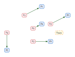
Remark 1 (Limitations of the Assignment Formulation).

The assignment problem has three key limitations that motivate the move to optimal transport:

Equal cardinality: it requires $| X | = | Y |$ .
No out-of-sample extension: a new point $x_{new}$ (Figure fig:sink:assignment) requires re-solving from scratch.
Cubic complexity: $O (n^{3})$ is prohibitive for the sample sizes ( $n \geq 10^{4}$ ) common in generative modelling.

Historical Note.

The problem of transporting mass at minimum cost was first posed by Gaspard Monge in 1781, who asked how to move a pile of earth to fill a hole of the same volume at minimum effort. In 1942, Leonid Kantorovich reformulated the problem by relaxing Monge's deterministic map to a probabilistic coupling, enabling linear-programming techniques. Kuhn [1] developed the Hungarian algorithm for the discrete case in 1955, crediting the Hungarian mathematicians König and Egerváry. For a historical account, see [2]. The modern computational breakthrough came from Cuturi [3], who showed that adding an entropic penalty reduces the complexity to near-linear time.

The Kantorovich Formulation

Kantorovich's insight was to replace Monge's deterministic map with a probabilistic coupling: instead of sending all the mass at $x_{i}$ to a single destination, we allow it to be split across multiple destinations.

Transport Plans and Couplings

Definition 2 (Kantorovich Optimal Transport).

Let $p \in ℝ_{+}^{n}$ and $q \in ℝ_{+}^{m}$ be discrete probability vectors (so $𝟙^{⊤} p = 𝟙^{⊤} q = 1$ ), and let $C \in ℝ_{+}^{n \times m}$ be a cost matrix with entry $C_{i j} = c (x_{i}, y_{j})$ . The coupling polytope is (Coupling) $\begin{matrix} Π (p, q) = {π \in ℝ_{+}^{n \times m} : π 𝟙_{m} = p, π^{⊤} 𝟙_{n} = q}, \end{matrix}$ and the optimal transport cost is (OT) $\begin{matrix} d_{c} (p, q) = \min_{π \in Π (p, q)} ⟨ C, π ⟩ = \min_{π \in Π (p, q)} \sum_{i, j} C_{i j} π_{i j} . \end{matrix}$ Each $π_{i j}$ represents the amount of mass moved from source $i$ to destination $j$ . The marginal constraints ensure that all mass is transported and all capacity is filled.

Proposition 1 (Existence of an Optimal Plan).

The coupling polytope $Π (p, q)$ is a non-empty, convex, and compact subset of $ℝ^{n \times m}$ . Consequently, the linear objective $⟨ C, π ⟩$ attains its minimum on $Π (p, q)$ , and an optimal transport plan always exists.

Proof.

Non-empty: The product distribution $π = p q^{⊤}$ satisfies both marginal constraints.

Convex: $Π (p, q)$ is the intersection of the non-negative orthant (convex) with affine hyperplanes (the marginal constraints), hence convex.

Compact: $Π (p, q) \subset {[0,1]}^{n \times m}$ (since all entries are non-negative and each row and column sums to at most $1$ ), so it is bounded. It is also closed (intersection of closed sets). Bounded and closed in $ℝ^{n m}$ implies compact.

Existence follows from the extreme value theorem: a continuous function on a compact set attains its minimum.

∎

Optimal transport allows mass splitting: source

a_{4}

sends mass to both

b_{1}

and

b_{3}

. Box sizes indicate mass; arrow thickness indicates flow. Conservation of mass ensures

\sum_{j} π_{i j} = a_{i}

(sources empty) and

\sum_{i} π_{i j} = b_{j}

(destinations fill).

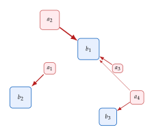
Example 1 (Wasserstein-1 as Optimal Transport).

When $X, Y \subset ℝ^{d}$ and $c (x, y) = ‖ x - y ‖$ , the optimal transport cost becomes the Wasserstein-1 distance: $W_{1} (p, q) = \min_{π \in Π (p, q)} \sum_{i, j} ‖ x_{i} - y_{j} ‖ π_{i j} .$ This is exactly the distance used in the WGAN objective (Chapter 10), providing the bridge between the GAN training loss and the transport-theoretic framework developed here.

OT as a Linear Program

Definition 3 (OT as Linear Program).

The Kantorovich problem is a linear program (LP) with $n m$ non-negative variables and $n + m$ equality constraints: (LP) $\begin{matrix} \min_{π \geq 0} ⟨ C, π ⟩ s.t. π 𝟙_{m} = p, π^{⊤} 𝟙_{n} = q . \end{matrix}$ Standard LP solvers (simplex, interior point) have worst-case complexity $O (n m (n + m) \log (n + m))$ , roughly cubic in $n$ when $n = m$ .

Kantorovich Duality

The LP has a dual that provides a powerful computational and theoretical tool.

Theorem 1 (Kantorovich Duality).

The optimal transport cost satisfies the strong duality relation (DUAL) $\begin{matrix} d_{c} (p, q) = \max_{𝒇, 𝒈} ⟨ 𝒇, p ⟩ + ⟨ 𝒈, q ⟩ s.t. f_{i} + g_{j} \leq C_{i j} \forall i, j, \end{matrix}$ where $𝒇 \in ℝ^{n}$ and $𝒈 \in ℝ^{m}$ are the dual variables (also called Kantorovich potentials).

Proof.

Equation is an LP in standard form. The primal is feasible (the product coupling $p q^{⊤} \in Π (p, q)$ ) and bounded below (all costs are non-negative). LP strong duality then gives . For full details, see any LP text [4].

∎

Remark 2 (Connection to the KR Dual).

When $c (x, y) = ‖ x - y ‖$ and both distributions are continuous, the constraint $f_{i} + g_{j} \leq ‖ x_{i} - y_{j} ‖$ reduces to $f$ being $1$ -Lipschitz (with $g = - f$ ), recovering the Kantorovich–Rubinstein representation $W_{1} (p, q) = \sup_{{‖ f ‖}_{L} \leq 1} 𝔼_{p} [f] - 𝔼_{q} [f]$ used in Chapter 10. The Sinkhorn approach developed below solves the primal instead.

Entropic Regularisation

The cubic complexity of LP solvers makes direct computation of $d_{c} (p, q)$ impractical for the sample sizes common in machine learning ( $n \geq 10^{4}$ ). Cuturi [3] observed that adding a small entropy penalty to the objective yields a problem that can be solved in near-linear time.

Definition 4 (Entropy-Regularised OT).

For a regularisation parameter $ϵ > 0$ , the entropy-regularised optimal transport cost is (Entot) $\begin{matrix} d_{c}^{ϵ} (p, q) = \min_{π \in Π (p, q)} ⟨ C, π ⟩ - ϵ H (π), \end{matrix}$ where $H (π) = - \sum_{i, j} π_{i j} \log π_{i j}$ is the (discrete) entropy of the plan.

Proposition 2 (Unique Optimal Plan).

The objective in is $ϵ$ -strongly convex, so the entropy-regularised problem has a unique minimiser $π_{ϵ}^{*} \in Π (p, q)$ .

Proof.

The linear term $⟨ C, π ⟩$ is convex (linear). The negative entropy $- H (π) = \sum_{i, j} π_{i j} \log π_{i j}$ has Hessian $\frac{\partial^{2} (- H)}{\partial π_{i j}^{2}} = \frac{1}{π_{i j}} > 0$ on the interior of $Π (p, q)$ . Since $π_{i j} \in (0,1)$ , we have $\frac{1}{π_{i j}} > 1$ , so $- H$ is $1$ -strongly convex with respect to the $ℓ_{1}$ norm. Scaling by $ϵ$ gives $ϵ$ -strong convexity of the full objective. A strongly convex function on a compact convex set has a unique minimiser.

∎

Proposition 3 (Limiting Behaviour).

As $ϵ \to 0^{+}$ , $d_{c}^{ϵ} (p, q) \to d_{c} (p, q)$ and $π_{ϵ}^{*}$ converges to the maximum-entropy optimal plan.
As $ϵ \to \infty$ , $π_{ϵ}^{*} \to p q^{⊤}$ (the product coupling), and $d_{c}^{ϵ} (p, q) \to ⟨ C, p q^{⊤} ⟩ - ϵ H (p q^{⊤})$ .

Proof.

Part (i): As $ϵ \to 0$ , the entropy penalty vanishes, so any minimiser of must also minimise $⟨ C, π ⟩$ on $Π (p, q)$ . Among the (possibly multiple) LP optima, the limit selects the one with maximum entropy (a consequence of $Γ$ -convergence of the regularised objective to the unregularised one).

Part (ii): As $ϵ \to \infty$ , the objective is dominated by $- ϵ H (π)$ , so the minimiser maximises entropy. Among all couplings with marginals $p$ and $q$ , the maximum-entropy coupling is the independent coupling $p q^{⊤}$ (by the product rule for entropy: $H (p q^{⊤}) = H (p) + H (q) \geq H (π)$ for any $π \in Π (p, q)$ , with equality iff $π = p q^{⊤}$ ).

∎

Reformulation as KL Projection

Define the Gibbs kernel (Gibbs) $\begin{matrix} K_{i j} = e^{- C_{i j} / ϵ}, \overline{K} = \frac{K}{Z_{ϵ}}, Z_{ϵ} = \sum_{i, j} K_{i j}, \end{matrix}$ so that $\overline{K}$ is a probability distribution on ${1, \dots, n} \times {1, \dots, m}$ . We now show that the entropy-regularised problem reduces to a KL projection.

Proposition 4 (Entropic OT as KL Minimisation).

(KL) $\begin{matrix} {arg min}_{π \in Π (p, q)} ⟨ C, π ⟩ - ϵ H (π) = {arg min}_{π \in Π (p, q)} 𝖣_{KL} (π ‖ \overline{K}) . \end{matrix}$

Proof.

Expanding the KL divergence: $\begin{matrix} 𝖣_{KL} (π ‖ \overline{K}) & = \sum_{i, j} π_{i j} \log \frac{π_{i j}}{{\overline{K}}_{i j}} \\ = \sum_{i, j} π_{i j} \log π_{i j} - \sum_{i, j} π_{i j} \log {\overline{K}}_{i j} \\ = - H (π) - \sum_{i, j} π_{i j} (- \frac{C_{i j}}{ϵ} - \log Z_{ϵ}) \\ = - H (π) + \frac{1}{ϵ} ⟨ C, π ⟩ + \log Z_{ϵ} . \end{matrix}$ Since $\log Z_{ϵ}$ is independent of $π$ , minimising $𝖣_{KL} (π ‖ \overline{K})$ over $Π (p, q)$ is equivalent to minimising $\frac{1}{ϵ} ⟨ C, π ⟩ - H (π)$ , which is $\frac{1}{ϵ}$ times the objective in .

∎

The Sinkhorn Algorithm

The KL reformulation reveals that the entropy-regularised problem is a projection of $\overline{K}$ onto the intersection of two affine sets: the row-marginal constraint $Π (p) = {π : π 𝟙_{m} = p}$ and the column-marginal constraint $Π (q) = {π : π^{⊤} 𝟙_{n} = q}$ , so that $Π (p, q) = Π (p) \cap Π (q)$ . This is precisely the setting of alternating Bregman projections.

Alternating KL Projections

Definition 5 (Marginal Constraint Sets).

(PIP) $\begin{matrix} Π (p) & = {π \in ℝ_{+}^{n \times m} : π 𝟙_{m} = p}, \\ Π (q) & = {π \in ℝ_{+}^{n \times m} : π^{⊤} 𝟙_{n} = q} . \end{matrix}$ Both are affine subsets of $ℝ^{n \times m}$ .

The alternating projection scheme initialises $π^{(0)} = \overline{K}$ and iterates: (Altproj) $\begin{matrix} π^{(ℓ + 1)} = {\begin{matrix} {arg min}_{π \in Π (p)} 𝖣_{KL} (π ‖ π^{(ℓ)}) & ℓ even (row projection), \\ {arg min}_{π \in Π (q)} 𝖣_{KL} (π ‖ π^{(ℓ)}) & ℓ odd (column projection) . \end{matrix} \end{matrix}$

Closed-Form Projections

Proposition 5 (Row Projection).

The KL projection onto $Π (p)$ is (Rowproj) $\begin{matrix} π_{i j}^{(2 ℓ)} = \frac{p_{i}}{\sum_{k} π_{i k}^{(2 ℓ - 1)}} π_{i j}^{(2 ℓ - 1)} . \end{matrix}$ In matrix form: $π^{(2 ℓ)} = diag (p ⊘ (π^{(2 ℓ - 1)} 𝟙_{m})) π^{(2 ℓ - 1)}$ , where $⊘$ denotes element-wise division.

Proof.

We minimise $𝖣_{KL} (π ‖ π^{(2 ℓ - 1)})$ subject to $π 𝟙_{m} = p$ . Introducing Lagrange multipliers $𝒇 \in ℝ^{n}$ : $ℒ (π, 𝒇) = \sum_{i, j} π_{i j} \log \frac{π_{i j}}{π_{i j}^{(2 ℓ - 1)}} + \sum_{i} f_{i} (p_{i} - \sum_{j} π_{i j}) .$ Setting $\frac{\partial ℒ}{\partial π_{i j}} = 0$ : $1 + \log π_{i j} - \log π_{i j}^{(2 ℓ - 1)} - f_{i} = 0 ⟹ π_{i j} = e^{f_{i} - 1} π_{i j}^{(2 ℓ - 1)} .$ Summing over $j$ and using the constraint $\sum_{j} π_{i j} = p_{i}$ : $p_{i} = e^{f_{i} - 1} \sum_{j} π_{i j}^{(2 ℓ - 1)} ⟹ e^{f_{i} - 1} = \frac{p_{i}}{\sum_{j} π_{i j}^{(2 ℓ - 1)}} .$ Substituting back gives .

∎

By an identical argument with roles of rows and columns swapped:

Proposition 6 (Column Projection).

The KL projection onto $Π (q)$ is (Colproj) $\begin{matrix} π_{i j}^{(2 ℓ + 1)} = \frac{q_{j}}{\sum_{k} π_{k j}^{(2 ℓ)}} π_{i j}^{(2 ℓ)} . \end{matrix}$ In matrix form: $π^{(2 ℓ + 1)} = π^{(2 ℓ)} diag (q ⊘ (π^{(2 ℓ) ⊤} 𝟙_{n}))$ .

Matrix Scaling Form

The alternating projections suggest a diagonal scaling structure.

Theorem 2 (Sinkhorn Factorisation).

The entropy-regularised optimal plan has the form (Factor) $\begin{matrix} π_{ϵ}^{*} = diag (𝒖^{*}) K diag (𝒗^{*}), \end{matrix}$ for unique vectors $𝒖^{*} \in ℝ_{> 0}^{n}$ , $𝒗^{*} \in ℝ_{> 0}^{m}$ , where $K_{i j} = e^{- C_{i j} / ϵ}$ .

Proof.

Consider the full Lagrangian of with dual variables $𝒇 \in ℝ^{n}$ (row marginals) and $𝒈 \in ℝ^{m}$ (column marginals): $ℒ (π, 𝒇, 𝒈) = \sum_{i, j} C_{i j} π_{i j} + ϵ \sum_{i, j} π_{i j} \log π_{i j} + \sum_{i} f_{i} (p_{i} - \sum_{j} π_{i j}) + \sum_{j} g_{j} (q_{j} - \sum_{i} π_{i j}) .$ Setting $\frac{\partial ℒ}{\partial π_{i j}} = 0$ : $\begin{matrix} C_{i j} + ϵ (1 + \log π_{i j}) - f_{i} - g_{j} & = 0, \\ \log π_{i j} & = \frac{f_{i}}{ϵ} - \frac{1}{2} + \frac{g_{j}}{ϵ} - \frac{1}{2} - \frac{C_{i j}}{ϵ}, \\ π_{i j} & = \underset{u_{i}}{\underset{⏟}{e^{f_{i} / ϵ - 1 / 2}}} \underset{K_{i j}}{\underset{⏟}{e^{- C_{i j} / ϵ}}} \underset{v_{j}}{\underset{⏟}{e^{g_{j} / ϵ - 1 / 2}}} . \end{matrix}$ Defining $u_{i} = e^{f_{i} / ϵ - 1 / 2}$ and $v_{j} = e^{g_{j} / ϵ - 1 / 2}$ , we obtain $π_{i j} = u_{i} K_{i j} v_{j}$ , which in matrix form is $π = diag (𝒖) K diag (𝒗)$ . The vectors $𝒖, 𝒗$ are strictly positive since the exponential function is positive. Uniqueness (up to a common scalar) follows from the strict convexity of the objective.

∎

Theorem 3 (Sinkhorn Iterations).

Initialise $𝒗^{(0)} = 𝟙_{m}$ . The iterations (Iterations) $\begin{matrix} 𝒖^{(ℓ + 1)} = p ⊘ (K 𝒗^{(ℓ)}), 𝒗^{(ℓ + 1)} = q ⊘ (K^{⊤} 𝒖^{(ℓ + 1)}), \end{matrix}$ converge to the unique $(𝒖^{*}, 𝒗^{*})$ satisfying $π_{ϵ}^{*} = diag (𝒖^{*}) K diag (𝒗^{*})$ . The resulting sequence of plans $π^{(ℓ)} = diag (𝒖^{(ℓ)}) K diag (𝒗^{(ℓ)})$ recovers the alternating projections –.

Proof.

We show by induction that the dual iterates $(𝒖^{(ℓ)}, 𝒗^{(ℓ)})$ produce the same plans as the primal alternating projections. Write ${\tilde{π}}^{(ℓ)} = diag (𝒖^{(ℓ)}) K diag (𝒗^{(ℓ)})$ .

Row update. Starting from ${\tilde{π}}^{(2 ℓ - 1)} = diag (𝒖^{(ℓ)}) K diag (𝒗^{(ℓ)})$ , the row projection gives: $\begin{matrix} {\tilde{π}}^{(2 ℓ)} & = diag (p ⊘ ({\tilde{π}}^{(2 ℓ - 1)} 𝟙_{m})) {\tilde{π}}^{(2 ℓ - 1)} \\ = diag (p ⊘ (diag (𝒖^{(ℓ)}) K 𝒗^{(ℓ)})) diag (𝒖^{(ℓ)}) K diag (𝒗^{(ℓ)}) \\ = diag (𝒖^{(ℓ + 1)}) K diag (𝒗^{(ℓ)}), \end{matrix}$ where $𝒖^{(ℓ + 1)} = p ⊘ (K 𝒗^{(ℓ)})$ .

Column update. Similarly, the column projection gives ${\tilde{π}}^{(2 ℓ + 1)} = diag (𝒖^{(ℓ + 1)}) K diag (𝒗^{(ℓ + 1)})$ with $𝒗^{(ℓ + 1)} = q ⊘ (K^{⊤} 𝒖^{(ℓ + 1)})$ .

Convergence follows from the general theory of alternating Bregman projections onto affine sets [5]: the iterates converge to the unique point in $Π (p) \cap Π (q)$ that is closest to $\overline{K}$ in KL divergence.

∎

Algorithm 1 (Sinkhorn Algorithm).

Input: cost matrix $C \in ℝ_{+}^{n \times m}$ , marginals $p \in ℝ_{+}^{n}$ , $q \in ℝ_{+}^{m}$ , regularisation $ϵ > 0$ , iterations $L$ . Output: approximate transport plan $π \in ℝ^{n \times m}$ .

Compute the Gibbs kernel: $K_{i j} \leftarrow e^{- C_{i j} / ϵ}$ .
Initialise $𝒗 \leftarrow 𝟙_{m}$ .
For $ℓ = 1, \dots, L$ : enumerate
$𝒖 \leftarrow p ⊘ (K 𝒗)$ (row normalisation)
$𝒗 \leftarrow q ⊘ (K^{⊤} 𝒖)$ (column normalisation) enumerate
Return $π \leftarrow diag (𝒖) K diag (𝒗)$ .

Each iteration costs $O (n m)$ (two matrix–vector products), so the total complexity is $O (L n m)$ , near-linear when $L$ is a small constant.

Proposition 7 (Linear Convergence).

The Sinkhorn iterates converge linearly: there exists a contraction rate $ρ \in (0,1)$ , depending on $ϵ$ and the cost matrix $C$ , such that ${‖ 𝒖^{(ℓ)} - 𝒖^{*} ‖}_{\infty} = O (ρ^{ℓ}), {‖ 𝒗^{(ℓ)} - 𝒗^{*} ‖}_{\infty} = O (ρ^{ℓ}) .$ In practice, $L = 50$ – $100$ iterations suffice for high accuracy. As $ϵ \to 0$ , the rate $ρ \to 1$ and more iterations are needed; as $ϵ \to \infty$ , $ρ \to 0$ (instant convergence to the product coupling).

Example 2 (Worked $3 \times 3$ Example).

Let $p = (\frac{1}{3}, \frac{1}{3}, \frac{1}{3})$ , $q = (\frac{1}{2}, \frac{1}{4}, \frac{1}{4})$ , $ϵ = 1$ , and $C = (\begin{matrix} 0 & 1 & 2 \\ 1 & 0 & 1 \\ 2 & 1 & 0 \end{matrix}), K = e^{- C / ϵ} = (\begin{matrix} 1 & e^{- 1} & e^{- 2} \\ e^{- 1} & 1 & e^{- 1} \\ e^{- 2} & e^{- 1} & 1 \end{matrix}) \approx (\begin{matrix} 1 & 0.368 & 0.135 \\ 0.368 & 1 & 0.368 \\ 0.135 & 0.368 & 1 \end{matrix}) .$ Starting from $𝒗^{(0)} = (1, 1, 1)$ :

$𝒖^{(1)} = p ⊘ (K 𝒗^{(0)}) = \frac{1}{3} (1 / 1.503, 1 / 1.736, 1 / 1.503) \approx (0.222, 0.192, 0.222)$ .
$𝒗^{(1)} = q ⊘ (K^{⊤} 𝒖^{(1)})$ , and so on.

After $L = 20$ iterations the marginal violation is about $2 \times 10^{- 11}$ , so the plan $π^{(L)}$ reproduces $p$ and $q$ to roughly eleven decimal places. True machine precision in double arithmetic (around $10^{- 16}$ ) takes about $L = 30$ here. The gap between those two figures is a useful calibration: convergence is linear, so each additional handful of iterations buys several more digits, and $ϵ = 1$ is large relative to the costs $0, 1, 2$ in this instance, which makes the contraction unusually fast. Harder instances with smaller $ϵ$ need the $L = 50$ to $100$ quoted in Proposition Proposition 7.

Sinkhorn Divergence

The entropy-regularised cost $d_{c}^{ϵ} (p, q)$ has a subtle defect: it does not vanish when $p = q$ . Two separate effects are at work, and it is worth keeping them apart.

First, the entropy term rewards spreading, so the optimal plan is no longer the identity coupling even when the two distributions are the same, and the transport bill $⟨ C, π_{ϵ}^{*} ⟩$ is therefore strictly positive where the unregularised optimum was zero. Second, the objective subtracts $ϵ H (π)$ , and since $H \geq 0$ this pushes the reported value down: with $p = q = (\frac{1}{2}, \frac{1}{2})$ , $C = (\begin{matrix} 0 & 1 \\ 1 & 0 \end{matrix})$ and $ϵ = 1$ , the optimum has $⟨ C, π_{ϵ}^{*} ⟩ = 0.2689$ and $H = 1.2753$ , giving $d_{c}^{ϵ} (p, p) = - 1.0064$ .

So $d_{c}^{ϵ} (p, p) \neq 0$ , which is all the defect requires, but the sign depends on which term dominates and is not in general positive. This is why the repair below subtracts the two self-comparison terms rather than simply shifting by a constant.

Definition 6 (Sinkhorn Divergence).

The Sinkhorn divergence [6] is the debiased quantity (Divergence) $\begin{matrix} {\overline{S}}_{ϵ} (p, q) = d_{c}^{ϵ} (p, q) - \frac{1}{2} d_{c}^{ϵ} (p, p) - \frac{1}{2} d_{c}^{ϵ} (q, q) . \end{matrix}$

Proposition 8 (Properties of the Sinkhorn Divergence).

The Sinkhorn divergence satisfies:

Non-negativity: ${\overline{S}}_{ϵ} (p, q) \geq 0$ .
Identity of indiscernibles: ${\overline{S}}_{ϵ} (p, q) = 0$ if and only if $p = q$ .
Metrisation of weak convergence: ${\overline{S}}_{ϵ} (p_{n}, q) \to 0$ if and only if $p_{n} ⇀ q$ weakly.
Interpolation: as $ϵ \to 0$ , ${\overline{S}}_{ϵ} \to d_{c}$ (unregularised OT); as $ϵ \to \infty$ , ${\overline{S}}_{ϵ} \to {MMD}_{k}^{2}$ (the maximum mean discrepancy with kernel $k = - c$ ) [7].

Insight.

The unregularised Wasserstein distance $W_{1}$ suffers from a curse of dimensionality: estimating it from $n$ samples in $ℝ^{d}$ has error $O (n^{- 1 / d})$ , which is catastrophically slow for images ( $d \sim 10^{4}$ ). For the Sinkhorn divergence ${\overline{S}}_{ϵ}$ the situation is far better: the error decays at the dimension-free rate $O (n^{- 1 / 2})$ , so the exponent no longer degrades as $d$ grows. This is why entropic OT is the practical choice for generative modelling.

Be precise about what is and is not dimension-free here. It is the rate in $n$ . The constant is not: the bound of Genevay et al. [8] carries a factor $e^{κ / ϵ} (1 + ϵ^{- ⌊ d / 2 ⌋})$ , which grows with the dimension and blows up as $ϵ \to 0$ . So $ϵ$ is not a free parameter that can be sent to zero to recover unregularised OT while keeping the good rate; shrinking it trades the constant away. This is the statistical counterpart of the numerical tension described below, and it is why $ϵ$ is tuned rather than minimised.

Caution.

The regularisation parameter $ϵ$ requires careful tuning:

Too small ( $ϵ \to 0$ ): the Gibbs kernel $K = e^{- C / ϵ}$ has entries near $0$ or $1$ , causing numerical underflow and slow convergence.
Too large ( $ϵ \to \infty$ ): the optimal plan approaches the independent coupling $p q^{⊤}$ , losing all geometric information about the cost.

In practice, $ϵ$ is set to a small fraction of the median pairwise cost.

Sinkhorn Generative Modelling

We now show how the Sinkhorn algorithm provides a differentiable loss function for training a generative model.

Architecture and Loss

Let $G_{θ} : ℝ^{k} \to ℝ^{d}$ be a generator network with parameters $θ$ . Given a mini-batch of real samples ${y_{1}, \dots, y_{n}} \sim p_{data}$ and generated samples ${x_{1}, \dots, x_{m}}$ with $x_{i} = G_{θ} (z_{i})$ , $z_{i} \sim Normal (0, I_{k})$ , we compute the pairwise cost matrix $C_{i j} = c (x_{i}, y_{j})$ , run $L$ Sinkhorn iterations to obtain $(𝒖_{L}, 𝒗_{L})$ , and define the loss:

Definition 7 (Sinkhorn Generative Loss).

(Genloss) $\begin{matrix} {\hat{E}}_{L} (θ) = ⟨ (C ⊙ K) 𝒗_{L}, 𝒖_{L} ⟩, \end{matrix}$ where $⊙$ denotes the Hadamard (element-wise) product, and $𝒖_{L}, 𝒗_{L}$ are the Sinkhorn scaling vectors after $L$ iterations.

Key Idea.

The Sinkhorn iterations are a sequence of differentiable operations (matrix–vector products, element-wise divisions). Therefore, ${\hat{E}}_{L} (θ)$ is differentiable with respect to $θ$ , and we can backpropagate through all $L$ iterations to update the generator via gradient descent. No adversarial discriminator is needed; the Sinkhorn loss is a direct, critic-free measure of distributional distance.

Sinkhorn generative modelling architecture. The generator transforms latent samples into

{x_{i}}

; the Sinkhorn algorithm computes the transport loss between generated and real samples; gradients flow back through the Sinkhorn iterations to update

θ

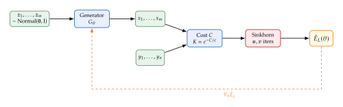
Algorithm 2 (Sinkhorn Generative Modelling).

Input: training data ${y^{(i)}}_{i = 1}^{N}$ , prior $p_{𝒛} = Normal (0, I)$ , regularisation $ϵ$ , Sinkhorn iterations $L$ , learning rate $η$ , epochs $T$ . Output: trained generator parameters $θ$ .

Initialise $θ$ randomly.
For $t = 1, \dots, T$ : enumerate
Sample mini-batch ${y_{1}, \dots, y_{n}}$ from training data.
Sample ${z_{1}, \dots, z_{m}} \sim p_{𝒛}$ and compute $x_{i} = G_{θ} (z_{i})$ .
Compute cost matrix: $C_{i j} = {‖ x_{i} - y_{j} ‖}^{2}$ .
Compute Gibbs kernel: $K_{i j} = e^{- C_{i j} / ϵ}$ .
Run $L$ Sinkhorn iterations (Algorithm Algorithm 1) to obtain $𝒖_{L}, 𝒗_{L}$ .
Compute loss: ${\hat{E}}_{L} (θ) = ⟨ (C ⊙ K) 𝒗_{L}, 𝒖_{L} ⟩$ .
Update: $θ \leftarrow θ - η \nabla_{θ} {\hat{E}}_{L} (θ)$ . enumerate

Remark 3 (Comparison with WGAN).

	WGAN	Sinkhorn
Distance	$W_{1}$ (KR dual)	$d_{c}^{ϵ}$ (primal)
Estimation	Critic network $f_{w}$	Direct matrix computation
Training	Min-max game	Single minimisation
Gradient	Through critic	Through Sinkhorn iters
Scalability	Any batch size	$O (L n m)$ per batch
Stability	Lipschitz enforcement	$ϵ$ tuning

The key advantage of Sinkhorn is the absence of adversarial training: there is no discriminator/critic to train, eliminating mode collapse from the discriminator side. The disadvantage is the

O (n m)

cost of the kernel matrix, which limits batch sizes.

Computational Aspects and Extensions

Log-Domain Sinkhorn

Remark 4 (Numerical Stability).

When $ϵ$ is small, the Gibbs kernel entries $K_{i j} = e^{- C_{i j} / ϵ}$ can underflow to zero, causing division-by-zero in the Sinkhorn iterations. The log-domain formulation works entirely in $(\log u, \log v)$ space: (U) $\begin{matrix} \log u_{i}^{(ℓ + 1)} & = \log p_{i} - {logsumexp}_{j} (\log v_{j}^{(ℓ)} - C_{i j} / ϵ), \\ \log v_{j}^{(ℓ + 1)} & = \log q_{j} - {logsumexp}_{i} (\log u_{i}^{(ℓ + 1)} - C_{i j} / ϵ), \end{matrix}$ where $logsumexp$ prevents over/underflow by working in log space throughout. This is essential for small $ϵ$ .

Mini-Batch Optimal Transport

In practice, the cost matrix $C \in ℝ^{n \times m}$ is computed from mini-batches of size $n, m \sim 64$ – $512$ . The mini-batch Sinkhorn loss approximates the population-level Sinkhorn divergence: ${\overline{S}}_{ϵ} (p_{data}, p_{θ}) \approx {\overline{S}}_{ϵ} ({\hat{p}}_{n}, {\hat{p}}_{m}),$ where ${\hat{p}}_{n} = \frac{1}{n} \sum_{i = 1}^{n} δ_{y_{i}}$ and ${\hat{p}}_{m} = \frac{1}{m} \sum_{i = 1}^{m} δ_{x_{i}}$ . Using the debiased Sinkhorn divergence instead of the raw entropic cost is critical here, as it eliminates the bias that would otherwise accumulate across mini-batches.

Extensions

Remark 5 (Unbalanced Optimal Transport).

When the total masses of $p$ and $q$ differ (e.g., in point cloud registration or partial matching), the marginal constraints are relaxed using KL penalties: $\min_{π \geq 0} ⟨ C, π ⟩ - ϵ H (π) + τ_{1} 𝖣_{KL} (π 𝟙 ‖ p) + τ_{2} 𝖣_{KL} (π^{⊤} 𝟙 ‖ q),$ where $τ_{1}, τ_{2} > 0$ control how strictly the marginals are enforced. The Sinkhorn-like iterations for unbalanced OT involve an additional softmax damping step.

Remark 6 (Connection to Schrödinger Bridges).

The entropy-regularised OT problem is equivalent to the Schrödinger bridge problem: find the most likely stochastic process connecting distribution $p$ at time $0$ to distribution $q$ at time $1$ , given a reference Brownian motion. The Sinkhorn iterations correspond to the iterative proportional fitting (IPF) algorithm for Schrödinger bridges. This connection has recently inspired diffusion Schrödinger bridges, linking optimal transport to score-based diffusion models.

Method	Complexity	Regularised?	Differentiable?
Hungarian algorithm	$O (n^{3})$	No	No
LP (simplex)	$O (n^{3} \log n)$	No	No
Auction algorithm	$O (n^{2} \log n)$	No	No
Sinkhorn	$O (L n^{2})$	Yes ( $ϵ$ )	Yes
Log-domain Sinkhorn	$O (L n^{2})$	Yes	Yes (stable)

Historical Note.

The Sinkhorn algorithm predates its use in machine learning by decades. Richard Sinkhorn proved in 1964 that alternating row and column normalisation of a positive matrix converges to a doubly stochastic matrix. Cuturi [3] connected this to optimal transport in 2013, showing that the Sinkhorn iteration solves the entropy-regularised OT problem and scales to thousands of points. Genevay et al. [6] introduced the debiased Sinkhorn divergence and demonstrated its use as a loss function for generative models. Feydy et al. [7] showed that Sinkhorn divergences interpolate between OT distances and kernel MMD, unifying two major families of distributional distances.

Exercises

Exercise 1 (Transport Plan Constraints).

Let $p = (\frac{1}{3}, \frac{1}{3}, \frac{1}{3})$ and $q = (\frac{1}{2}, \frac{1}{4}, \frac{1}{4})$ on three points with cost matrix $C = (\begin{matrix} 0 & 1 & 2 \\ 1 & 0 & 1 \\ 2 & 1 & 0 \end{matrix})$ . Write down all constraints that $π \in Π (p, q)$ must satisfy. How many free variables does $π$ have after the marginal constraints? Find the optimal transport plan by inspection or by solving the LP.

Exercise 2 (Compactness of the Coupling Polytope).

Prove that $Π (p, q) = {π \geq 0 : π 𝟙_{m} = p, 𝟙_{n}^{⊤} π = q}$ is convex and compact. Use this to prove that the OT problem always has a solution. Hint: $Π (p, q)$ is a bounded, closed subset of $ℝ^{n m}$ .

Exercise 3 (Entropy Limit Behaviour).

Show that as $ϵ \to \infty$ , the entropy-regularised optimal plan $π_{ϵ}^{*}$ converges to the product coupling $p q^{⊤}$ . Hint: the product coupling uniquely maximises $H (π)$ over $Π (p, q)$ . What does $d_{c}^{ϵ} (p, q)$ converge to?

Exercise 4 (Sinkhorn Marginal Satisfaction).

Starting from $𝒖^{(0)} = 𝟙_{n}$ and $𝒗^{(0)} = 𝟙_{m}$ , show that after the first row update $𝒖^{(1)} = p ⊘ (K 𝒗^{(0)})$ , the plan $π^{(1)} = diag (𝒖^{(1)}) K diag (𝒗^{(0)})$ satisfies $π^{(1)} 𝟙_{m} = p$ exactly. Does it satisfy ${(π^{(1)})}^{⊤} 𝟙_{n} = q$ ?

Exercise 5 (Birkhoff–von Neumann and OT).

A doubly stochastic matrix has all row and column sums equal to $1$ . The Birkhoff–von Neumann theorem states that the set of $n \times n$ doubly stochastic matrices is the convex hull of permutation matrices. Show that when $p = q = \frac{1}{n} 𝟙_{n}$ , the coupling polytope $Π (p, q) = \frac{1}{n} ℬ_{n}$ where $ℬ_{n}$ is the Birkhoff polytope. What does the unregularised optimal plan correspond to in this case?

Exercise 6 (Backpropagation Through Sinkhorn).

In Sinkhorn generative modelling, the loss ${\hat{E}}_{L} (θ) = ⟨ (C ⊙ K) 𝒗_{L}, 𝒖_{L} ⟩$ depends on $θ$ through the cost matrix $C_{i j} = c (G_{θ} (z_{i}), y_{j})$ . Argue that each Sinkhorn iteration (element-wise division, matrix–vector product) is composed of differentiable operations, so $\nabla_{θ} {\hat{E}}_{L} (θ)$ can be computed by automatic differentiation through all $L$ iterations. What is the memory cost of storing all intermediate $𝒖^{(ℓ)}, 𝒗^{(ℓ)}$ for backpropagation?

Exercise 7 (WGAN vs. Sinkhorn).

Compare WGAN and Sinkhorn-based generative models along these axes:

How does each estimate the Wasserstein distance?
Which requires adversarial training, and why?
What are the computational bottlenecks of each?
In what regime (small $n$ vs. large $n$ ) is each preferred?

Exercise 8 (Log-Domain Stability).

For $ϵ = 0.01$ and $C_{i j} \in [0, 10]$ , show that the Gibbs kernel entry $K_{i j} = e^{- C_{i j} / ϵ}$ can be as small as $e^{- 1000} \approx 10^{- 434}$ , which underflows in double-precision floating point (minimum $\approx 10^{- 308}$ ). Verify that the log-domain update – avoids this issue.

Exercise 9 (Sinkhorn Divergence Debiasing).

Compute $d_{c}^{ϵ} (p, p)$ for $p = (\frac{1}{2}, \frac{1}{2})$ with cost $C = (\begin{matrix} 0 & 1 \\ 1 & 0 \end{matrix})$ and $ϵ = 1$ . Verify that $d_{c}^{ϵ} (p, p) \neq 0$ , confirming the bias of the raw entropic cost. Compute the debiased Sinkhorn divergence ${\overline{S}}_{ϵ} (p, p)$ and verify it equals zero.

Exercise 10 (Kantorovich Duality Verification).

For $p = (\frac{1}{2}, \frac{1}{2})$ , $q = (1)$ (a single point), and $c (x_{i}, y_{1}) = | x_{i} - y_{1} |$ with $x_{1} = 0$ , $x_{2} = 1$ , $y_{1} = 0.5$ :

Solve the primal OT problem directly (there is only one feasible plan).
Find dual potentials $(f_{1}, f_{2}, g_{1})$ satisfying complementary slackness and verify strong duality.

Exercise 11 (Convergence Rate and $ϵ$ ).

Run the Sinkhorn algorithm for the $3 \times 3$ example of Example Example 2 with $ϵ \in {0.01, 0.1, 1, 10}$ . For each $ϵ$ , record the number of iterations $L^{*}$ needed to achieve ${‖ π^{(L)} 𝟙 - p ‖}_{\infty} < 10^{- 6}$ . Verify empirically that $L^{*}$ increases as $ϵ \to 0$ . What happens to the optimal plan as $ϵ \to 0$ ?

Exercise 12 (Sample Complexity).

The unregularised $W_{1}$ distance has sample complexity $O (n^{- 1 / d})$ in dimension $d$ . Explain why this is prohibitively slow for images ( $d \sim 10^{4}$ ). The Sinkhorn divergence ${\overline{S}}_{ϵ}$ has sample complexity $O (n^{- 1 / 2})$ , independent of $d$ . Explain intuitively why the entropic regularisation “smooths out” the curse of dimensionality. Hint: the Gibbs kernel $K = e^{- C / ϵ}$ acts like a soft nearest-neighbour kernel.

References

The Hungarian method for the assignment problem

H. W. Kuhn

Naval Research Logistics Quarterly, vol. 2, no. 1-2, pp. 83-97 · 1955

BibTeX

@article{kuhn1955,
author = {Kuhn, H. W.},
title = {The Hungarian method for the assignment problem},
journal = {Naval Research Logistics Quarterly},
volume = {2},
number = {1-2},
pages = {83-97},
doi = {https://doi.org/10.1002/nav.3800020109},
url = {https://onlinelibrary.wiley.com/doi/abs/10.1002/nav.3800020109},
eprint = {https://onlinelibrary.wiley.com/doi/pdf/10.1002/nav.3800020109},
abstract = {Abstract Assuming that numerical scores are available for the performance of each of n persons on each of n jobs, the “assignment problem” is the quest for an assignment of persons to jobs so that the sum of the n scores so obtained is as large as possible. It is shown that ideas latent in the work of two Hungarian mathematicians may be exploited to yield a new method of solving this problem.},
year = {1955}
}

Journal article

A tale of three eras: The discovery and rediscovery of the Hungarian Method

Harold W. Kuhn

European Journal of Operational Research, vol. 219, no. 3, pp. 641-651 · 2012

BibTeX

@article{KUHN2012641,
title = {A tale of three eras: The discovery and rediscovery of the Hungarian Method},
journal = {European Journal of Operational Research},
volume = {219},
number = {3},
pages = {641-651},
year = {2012},
note = {Feature Clusters},
issn = {0377-2217},
doi = {https://doi.org/10.1016/j.ejor.2011.11.008},
url = {https://www.sciencedirect.com/science/article/pii/S0377221711009957},
author = {Harold W. Kuhn},
keywords = {Assignment, Combinatorial optimization, Graph theory, Linear programing, Hungarian Method}
}

Journal article

Sinkhorn Distances: Lightspeed Computation of Optimal Transport

Marco Cuturi

Advances in Neural Information Processing Systems · 2013

BibTeX

@inproceedings{cuturi2013sinkhorn,
  title={Sinkhorn Distances: Lightspeed Computation of Optimal Transport},
  author={Cuturi, Marco},
  booktitle={Advances in Neural Information Processing Systems},
  year={2013}
}

Conference paper

Linear Programming: Foundations and Extensions

Robert J. Vanderbei

Kluwer Academic Publishers · 1998

BibTeX

@book{vanderbei1998,
  title={Linear Programming: Foundations and Extensions},
  author={Vanderbei, Robert J.},
  publisher={Kluwer Academic Publishers},
  year={1998},
  address={Boston, MA}
}

Book

Proximity Maps for Convex Sets

Ward Cheney, Allen A. Goldstein

Proceedings of the American Mathematical Society, vol. 10, no. 3, pp. 448-450 · 1959

BibTeX

@article{Cheney1959ProximityMF,
  title={Proximity Maps for Convex Sets},
  author={Cheney, Ward and Goldstein, Allen A.},
  journal={Proceedings of the American Mathematical Society},
  volume={10},
  number={3},
  pages={448--450},
  year={1959},
  publisher={American Mathematical Society}
}

Journal article

Learning Generative Models with Sinkhorn Divergences

Aude Genevay, Gabriel Peyre, Marco Cuturi

Proceedings of the International Conference on Artificial Intelligence and Statistics (AISTATS) · 2018

BibTeX

@inproceedings{genevay2018learning,
  title={Learning Generative Models with Sinkhorn Divergences},
  author={Genevay, Aude and Peyr{\'e}, Gabriel and Cuturi, Marco},
  booktitle={Proceedings of the International Conference on Artificial
             Intelligence and Statistics (AISTATS)},
  year={2018}
}

Conference paper

Interpolating between Optimal Transport and MMD using Sinkhorn Divergences

Jean Feydy, Thibault Sejourne, Francois-Xavier Vialard, Shun-ichi Amari, Alain Trouve, Gabriel Peyre

Proceedings of the International Conference on Artificial Intelligence and Statistics (AISTATS) · 2019

BibTeX

@inproceedings{feydy2019interpolating,
  title={Interpolating between Optimal Transport and {MMD} using
         Sinkhorn Divergences},
  author={Feydy, Jean and S{\'e}journ{\'e}, Thibault and
          Vialard, Fran{\c{c}}ois-Xavier and Amari, Shun-ichi and
          Trouv{\'e}, Alain and Peyr{\'e}, Gabriel},
  booktitle={Proceedings of the International Conference on Artificial
             Intelligence and Statistics (AISTATS)},
  year={2019}
}

Conference paper

Sample Complexity of Sinkhorn Divergences

Aude Genevay, Lenaic Chizat, Francis Bach, Marco Cuturi, Gabriel Peyre

Proceedings of the International Conference on Artificial Intelligence and Statistics (AISTATS) · 2019

BibTeX

@inproceedings{genevay2019sample,
  title={Sample Complexity of {S}inkhorn Divergences},
  author={Genevay, Aude and Chizat, L{\'e}na{\"i}c and Bach, Francis and
          Cuturi, Marco and Peyr{\'e}, Gabriel},
  booktitle={Proceedings of the International Conference on Artificial
             Intelligence and Statistics (AISTATS)},
  year={2019}
}

Conference paper

← 13 GANs for Vision 15 Variational Autoencoders →