16 Advanced VAE Variants

From VAEs to VAE Variants

In 15 we built the core variational autoencoder from the ground up: the evidence lower bound (ELBO), the reparameterisation trick, and the closed-form Gaussian KL divergence that makes training practical. The vanilla VAE is elegant, but it carries several well-known limitations.

Key Idea.

The standard VAE uses a mode-covering KL divergence that averages over modes, contributing to blurry samples. Its latent dimensions are typically entangled, offering little control over individual generative factors. It has no built-in mechanism for conditional generation, and it restricts the latent space to continuous variables, even when the data is naturally discrete. Each of these limitations sparked a family of architectural variants.

This chapter traces five such variants, each addressing a specific weakness:

$β$ -VAE (The -VAE: Disentangled Representations): a single hyperparameter change that encourages disentangled latent representations.
Conditional VAE (Conditional VAE): extending the VAE to generate data conditioned on side information such as class labels.
VQ-VAE (VQ-VAE: Vector Quantised Variational Autoencoder): replacing the continuous latent space with a learned discrete codebook.
VQ-GAN (VQ-GAN: Adversarial Codebook Learning): adding adversarial and perceptual losses to sharpen VQ-VAE outputs.
VQ-VAE-2 (VQ-VAE-2: Hierarchical Discrete Representations): a hierarchical extension with multiple codebook levels for high-resolution generation.

Historical Note.

The period from 2015 to 2019 saw an explosion of VAE variants. Within two years of Kingma and Welling [1], over a dozen architectures had appeared, each targeting a specific weakness of the original model. By 2021, discrete-latent models such as VQ-VAE had become backbone components in large-scale systems like DALL-E and Stable Diffusion, far beyond what the original VAE paper envisioned.

The $β$ -VAE: Disentangled Representations

What if we could learn a latent space where each dimension captures exactly one independent generative factor, such as colour, shape, or orientation? This is the promise of disentangled representations, and the $β$ -VAE achieves it with a remarkably simple modification to the standard ELBO.

Definition 1 ( $β$ -VAE Objective).

The $β$ -VAE objective is (BETA OBJ) $\begin{matrix} ℒ_{β} = 𝔼_{q_{ϕ} (𝒛 | 𝒙)} [\log p_{θ} (𝒙 | 𝒛)] - β 𝖣_{KL} (q_{ϕ} (𝒛 | 𝒙) ‖ p (𝒛)), \end{matrix}$ where $β > 0$ is a scalar hyperparameter that controls the strength of the KL regularisation relative to reconstruction.

Setting $β = 1$ recovers the standard VAE ELBO from 15. Increasing $β$ beyond $1$ places stronger pressure on the approximate posterior to match the prior, while decreasing $β$ below $1$ yields a “loosened” VAE that prioritises reconstruction fidelity.

Remark 1 ( $β = 1$ Recovers the Standard ELBO).

When $β = 1$ , (BETA OBJ) is exactly the evidence lower bound derived in The Evidence Lower Bound. Values $β < 1$ have also found use in practice: they produce sharper reconstructions at the cost of a less structured latent space.

Why does a larger $β$ encourage disentanglement? The intuition connects to the information bottleneck principle: by aggressively penalising the KL term, the encoder is forced to transmit only the most essential information about $𝒙$ through $𝒛$ . Under this pressure, the most “efficient” encoding aligns each latent dimension with an independent generative factor, producing an axis-aligned, factorial posterior.

Definition 2 (Disentangled Representation).

A latent representation $𝒛 = (z_{1}, \dots, z_{d})$ is disentangled with respect to a set of independent generative factors ${v_{1}, \dots, v_{d}}$ if each latent dimension $z_{i}$ is sensitive to changes in exactly one factor $v_{i}$ and invariant to all others.

Proposition 1 (Extreme $β$ Trade-off).

Consider the $β$ -VAE objective in (BETA OBJ).

As $β \to \infty$ , the optimal encoder satisfies $q_{ϕ} (𝒛 | 𝒙) \to p (𝒛)$ for all $𝒙$ , leading to posterior collapse: the latent code carries no information about the input.
As $β \to 0$ , the KL term vanishes and the model reduces to a deterministic autoencoder with no regularisation on the latent space.

Proof.

For part (i), suppose $β \to \infty$ . The objective becomes $ℒ_{β} = \underset{bounded above}{\underset{⏟}{𝔼_{q_{ϕ}} [\log p_{θ} (𝒙 | 𝒛)]}} - β \underset{\geq 0}{\underset{⏟}{𝖣_{KL} (q_{ϕ} ‖ p)}} .$ For $ℒ_{β}$ to remain finite as $β \to \infty$ , we need $𝖣_{KL} (q_{ϕ} (𝒛 | 𝒙) ‖ p (𝒛)) \to 0$ for every $𝒙$ . Since the KL divergence equals zero if and only if the two distributions are identical almost everywhere, this forces $q_{ϕ} (𝒛 | 𝒙) = p (𝒛)$ . But then $𝒛$ is independent of $𝒙$ , which is precisely posterior collapse (see Posterior Collapse).

For part (ii), setting $β = 0$ removes the KL penalty entirely, so the optimisation reduces to $\max_{ϕ, θ} 𝔼_{q_{ϕ}} [\log p_{θ} (𝒙 | 𝒛)]$ . Without regularisation, $q_{ϕ}$ can concentrate all mass on a single point $𝒛^{*} (𝒙)$ , recovering a deterministic autoencoder with no structure in the latent space.

∎

Insight.

The $β$ -VAE illustrates a fundamental tension in representation learning: compression versus reconstruction. A practitioner must choose $β$ to balance these goals. Typical values for disentanglement experiments lie in the range $β \in [4, 50]$ , depending on the dataset and the desired level of latent interpretability.

Historical Note.

Irina Higgins and colleagues at DeepMind introduced the $β$ -VAE in 2017 [2]. The idea was strikingly simple: change one hyperparameter. Yet it sparked an entire research direction on disentanglement metrics and benchmarks (dSprites, 3D Shapes). The subsequent debate over whether unsupervised disentanglement is even possible without inductive biases remains one of the liveliest topics in representation learning.

Conditional VAE

So far, both the VAE and the $β$ -VAE generate data unconditionally: we sample $𝒛$ from the prior and decode. But what if we want to generate a specific digit, a face with particular attributes, or an image from a text description? The Conditional VAE (CVAE) extends the framework to condition on side information $𝒚$ .

Definition 3 (Conditional VAE).

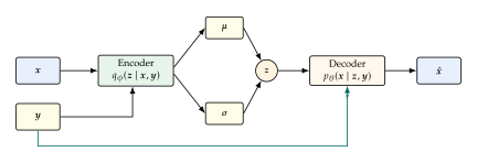
A Conditional VAE defines a generative model for data $𝒙$ given side information $𝒚$ through a latent variable $𝒛$ : (CVAE Model) $\begin{matrix} p_{θ} (𝒙 | 𝒚) = \int p_{θ} (𝒙 | 𝒛, 𝒚) p (𝒛) d 𝒛, \end{matrix}$ where $p (𝒛) = 𝒩 (0, I)$ is the prior over latents, and $p_{θ} (𝒙 | 𝒛, 𝒚)$ is the conditional decoder. The approximate posterior (encoder) is $q_{ϕ} (𝒛 | 𝒙, 𝒚)$ , which conditions on both the data and the side information.

The side information $𝒚$ can be a discrete class label, a continuous attribute vector, or even a natural language description. The key modelling choice is that $𝒚$ feeds into both the encoder and the decoder.

Theorem 1 (Conditional ELBO).

For any distribution $q_{ϕ} (𝒛 | 𝒙, 𝒚)$ with support containing that of $p_{θ} (𝒛 | 𝒙, 𝒚)$ , (CVAE ELBO) $\begin{matrix} \log p_{θ} (𝒙 | 𝒚) \geq 𝔼_{q_{ϕ} (𝒛 | 𝒙, 𝒚)} [\log p_{θ} (𝒙 | 𝒛, 𝒚)] - 𝖣_{KL} (q_{ϕ} (𝒛 | 𝒙, 𝒚) ‖ p (𝒛)) . \end{matrix}$ The gap between the left-hand side and the right-hand side equals $𝖣_{KL} (q_{ϕ} (𝒛 | 𝒙, 𝒚) ‖ p_{θ} (𝒛 | 𝒙, 𝒚))$ .

Proof.

The derivation mirrors the unconditional ELBO (The Evidence Lower Bound), with every term conditioned on $𝒚$ . Start from the log-marginal likelihood: (CVAE Jensen) $\begin{matrix} \log p_{θ} (𝒙 | 𝒚) & = \log \int p_{θ} (𝒙, 𝒛 | 𝒚) d 𝒛 \\ = \log \int \frac{p_{θ} (𝒙, 𝒛 | 𝒚)}{q_{ϕ} (𝒛 | 𝒙, 𝒚)} q_{ϕ} (𝒛 | 𝒙, 𝒚) d 𝒛 \\ \geq \int q_{ϕ} (𝒛 | 𝒙, 𝒚) \log \frac{p_{θ} (𝒙, 𝒛 | 𝒚)}{q_{ϕ} (𝒛 | 𝒙, 𝒚)} d 𝒛 \end{matrix}$ where the inequality in (CVAE Jensen) follows from Jensen's inequality applied to the concave logarithm. Expanding the joint $p_{θ} (𝒙, 𝒛 | 𝒚) = p_{θ} (𝒙 | 𝒛, 𝒚) p (𝒛)$ gives (CVAE ELBO Final) $\begin{matrix} RHS of & = 𝔼_{q_{ϕ} (𝒛 | 𝒙, 𝒚)} [\log p_{θ} (𝒙 | 𝒛, 𝒚)] + 𝔼_{q_{ϕ} (𝒛 | 𝒙, 𝒚)} [\log \frac{p (𝒛)}{q_{ϕ} (𝒛 | 𝒙, 𝒚)}] \\ = 𝔼_{q_{ϕ} (𝒛 | 𝒙, 𝒚)} [\log p_{θ} (𝒙 | 𝒛, 𝒚)] - 𝖣_{KL} (q_{ϕ} (𝒛 | 𝒙, 𝒚) ‖ p (𝒛)) . \end{matrix}$ For the gap, write $\begin{matrix} \log p_{θ} (𝒙 | 𝒚) - ELBO & = 𝔼_{q_{ϕ} (𝒛 | 𝒙, 𝒚)} [\log \frac{q_{ϕ} (𝒛 | 𝒙, 𝒚)}{p_{θ} (𝒛 | 𝒙, 𝒚)}] = 𝖣_{KL} (q_{ϕ} (𝒛 | 𝒙, 𝒚) ‖ p_{θ} (𝒛 | 𝒙, 𝒚)), \end{matrix}$ using Bayes' rule $p_{θ} (𝒛 | 𝒙, 𝒚) = p_{θ} (𝒙 | 𝒛, 𝒚) p (𝒛) / p_{θ} (𝒙 | 𝒚)$ . Since KL divergence is non-negative, the bound is tight when the approximate posterior equals the true posterior.

∎

Caution.

If the encoder ignores the side information and uses $q_{ϕ} (𝒛 | 𝒙)$ instead of $q_{ϕ} (𝒛 | 𝒙, 𝒚)$ , it cannot capture label-dependent variation in the latent space. The posterior approximation becomes suboptimal, and the bound loosens. In the worst case, the decoder learns to ignore $𝒚$ as well, and the model ceases to be a true conditional generative model.

Architecture of a Conditional VAE (CVAE). The side information

𝒚

feeds into both the encoder and the decoder. The encoder produces

q_{ϕ} (𝒛 | 𝒙, 𝒚)

, while the decoder reconstructs

𝒙

from both

𝒛

and

𝒚

Example 1 (Conditional MNIST Generation).

Consider training a CVAE on MNIST with $𝒚 \in {0, 1, \dots, 9}$ as the digit label. During training, the encoder receives both the image $𝒙$ and the one-hot label $𝒚$ , producing $q_{ϕ} (𝒛 | 𝒙, 𝒚)$ . The decoder reconstructs from $(𝒛, 𝒚)$ . At generation time, we fix $𝒚 = 7$ (say), sample $𝒛 \sim 𝒩 (0, I)$ , and decode: every sample is a plausible rendition of the digit $7$ , with variation in stroke width, slant, and style captured by the random $𝒛$ .

Historical Note.

Kihyuk Sohn, Honglak Lee, and Xinchen Yan introduced the Conditional VAE at NeurIPS 2015 [3]. A key insight of the paper was that conditioning the prior on $𝒚$ (i.e., using $p (𝒛 | 𝒚)$ instead of $p (𝒛)$ ) is possible but often unnecessary for practical applications. Conditioning only the encoder and decoder already allows the model to generate class-specific outputs while keeping the training procedure simple.

From Continuous to Discrete Latent Spaces

The VAE, $β$ -VAE, and CVAE all use continuous latent variables, typically drawn from a Gaussian. But many modalities are inherently discrete: language is composed of tokens, music consists of notes, and images can be described by a finite palette of visual patterns. Why not use a discrete latent space directly?

There is a deeper reason beyond matching data structure. Continuous latent codes produced by a Gaussian prior encourage the decoder to “average” nearby codes, which contributes to the characteristic blurriness of VAE samples. Discrete codes, by contrast, can index sharp prototypes in a learned codebook: each code maps to a single, well-defined embedding vector, eliminating the averaging effect.

Insight.

Discrete representations also align naturally with downstream tasks that require reasoning, planning, or symbolic manipulation. A finite codebook turns the latent space into a vocabulary, making it amenable to powerful sequence models such as autoregressive transformers and PixelCNNs.

The following table summarises the key differences between continuous and discrete latent variable models:

Property	Continuous VAE	Discrete VQ-VAE
Latent type	$𝒛 \in ℝ^{d}$	$𝒛 \in {1, \dots, K}$
Posterior	Gaussian $q_{ϕ} (𝒛 \| 𝒙)$	One-hot (deterministic)
KL divergence	Analytical (Gaussian KL)	Constant $\log K$
Gradient through $𝒛$	Reparameterisation trick	Straight-through estimator
Sample quality	Often blurry	Sharper (codebook prototypes)

Historical Note.

Vector quantisation itself is not a deep learning invention. Yoseph Linde, Andrés Buzo, and Robert Gray introduced the LBG algorithm for vector quantisation in 1980 [4], originally for speech coding and signal compression. Nearly four decades later, van den Oord and colleagues revived the idea within the deep generative modelling framework, combining classical VQ with neural encoders and decoders.

VQ-VAE: Vector Quantised Variational Autoencoder

The Vector Quantised VAE (VQ-VAE) replaces the continuous Gaussian latent space of a standard VAE with a discrete codebook of learnable embedding vectors. This section develops the full mathematical machinery.

Architecture

Definition 4 (VQ-VAE).

A VQ-VAE consists of three components:

An encoder $z_{e} (𝒙) \in ℝ^{d}$ that maps input $𝒙$ to a continuous embedding.
A codebook (embedding table) $ℰ = {𝒆_{1}, \dots, 𝒆_{K}} \subset ℝ^{d}$ of $K$ learnable prototype vectors.
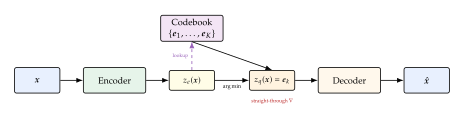
A quantisation step that maps the encoder output to the nearest codebook entry: (Quantise) $\begin{matrix} z_{q} (𝒙) = 𝒆_{k}, k = {arg min}_{j \in {1, \dots, K}} {‖ z_{e} (𝒙) - 𝒆_{j} ‖}_{2} . \end{matrix}$
A decoder $p_{θ} (𝒙 | z_{q})$ that reconstructs the input from the quantised code.

Definition 5 (Codebook).

The codebook $ℰ = {𝒆_{1}, \dots, 𝒆_{K}}$ is a learnable dictionary of $K$ prototype vectors in $ℝ^{d}$ . Each encoder output is “snapped” to its nearest codebook entry during the forward pass. The codebook can be thought of as a discrete “vocabulary” of latent representations, where each entry encodes a reusable visual or structural pattern.

Posterior and KL Divergence

Unlike the Gaussian VAE, where the posterior is a continuous density, the VQ-VAE posterior is a deterministic categorical distribution.

Proposition 2 (Deterministic Posterior and Constant KL).

In VQ-VAE, the posterior $q (𝒛 = k | 𝒙)$ is a one-hot distribution: $q (𝒛 = k | 𝒙) = {\begin{matrix} 1 & if k = {arg min}_{j} {‖ z_{e} (𝒙) - 𝒆_{j} ‖}_{2}, \\ 0 & otherwise . \end{matrix}$ With a uniform prior $p (𝒛) = 1 / K$ , the KL divergence is constant: $𝖣_{KL} (q (𝒛 | 𝒙) ‖ p (𝒛)) = \log K .$

Proof.

Since $q (𝒛 | 𝒙)$ places all its mass on a single index $k^{*}$ , the KL divergence reduces to $\begin{matrix} 𝖣_{KL} (q ‖ p) & = \sum_{k = 1}^{K} q (k | 𝒙) \log \frac{q (k | 𝒙)}{p (k)} = 1 \cdot \log \frac{1}{1 / K} = \log K, \end{matrix}$ where we used $q (k^{*} | 𝒙) = 1$ and $p (k^{*}) = 1 / K$ . All other terms vanish because $q (k | 𝒙) = 0$ for $k \neq k^{*}$ , and $0 \cdot \log (0 / p) = 0$ by convention.

∎

Since the KL is constant, it does not depend on the encoder parameters and drops out of the gradient computation. The training objective is therefore driven entirely by the reconstruction term and two auxiliary losses.

The VQ-VAE Loss Function

Definition 6 (VQ-VAE Loss).

The total VQ-VAE training loss is (Vqvae LOSS) $\begin{matrix} L = \underset{reconstruction}{\underset{⏟}{{‖ 𝒙 - \hat{𝒙} ‖}^{2}}} + \underset{codebook update}{\underset{⏟}{{‖ sg [z_{e} (𝒙)] - 𝒆 ‖}^{2}}} + \underset{commitment}{\underset{⏟}{β {‖ z_{e} (𝒙) - sg [𝒆] ‖}^{2}}}, \end{matrix}$ where $\hat{𝒙}$ is the decoder output, $𝒆$ is the selected codebook vector, and $sg [\cdot]$ denotes the stop-gradient operator.

Each of the three terms plays a distinct role. Let us examine the less familiar ones.

Remark 2 (The Stop-Gradient Operator).

The operator $sg [\cdot]$ acts as the identity during the forward pass but produces zero gradient during backpropagation. In PyTorch, this is implemented via x.detach(). The stop-gradient decouples the encoder and codebook updates: in the codebook loss ${‖ sg [z_{e} (𝒙)] - 𝒆 ‖}^{2}$ , gradients flow only to the codebook vectors $𝒆$ , while in the commitment loss ${‖ z_{e} (𝒙) - sg [𝒆] ‖}^{2}$ , gradients flow only to the encoder.

Remark 3 (Commitment Loss).

The commitment loss $β {‖ z_{e} (𝒙) - sg [𝒆] ‖}^{2}$ prevents the encoder outputs from growing unboundedly or drifting away from the codebook vectors. Without it, the encoder could produce embeddings in a region of $ℝ^{d}$ far from any codebook entry, making the quantisation step meaningless. The hyperparameter $β$ is typically set to $0.25$ .

Gradient Flow: The Straight-Through Estimator

The $arg min$ in (Quantise) is a discrete, non-differentiable operation. How do gradients from the decoder reach the encoder?

Proposition 3 (Straight-Through Estimator).

The straight-through estimator approximates the gradient of the quantisation step by copying the gradient of the decoder input directly to the encoder output: $\nabla_{z_{e}} L \approx \nabla_{z_{q}} L .$ That is, in the forward pass the discrete mapping $z_{e} \mapsto z_{q}$ is applied as usual, but in the backward pass the $arg min$ is treated as the identity function, allowing the decoder's gradient signal to flow unaltered back to the encoder.

This approximation is justified by the observation that the codebook and commitment losses keep $z_{e} (𝒙)$ and $𝒆$ close together, so the local geometry around $z_{e}$ and $z_{q}$ is similar. In practice, it works remarkably well, and VQ-VAE trains stably with standard optimisers.

Architecture of VQ-VAE. The encoder maps

𝒙

to a continuous embedding

z_{e} (𝒙)

, which is quantised to the nearest codebook vector

𝒆_{k}

. The decoder reconstructs from the quantised code. Gradients from the decoder pass through the quantisation step via the straight-through estimator.

Historical Note.

Aaron van den Oord, Oriol Vinyals, and Koray Kavukcuoglu at DeepMind introduced VQ-VAE in 2017 [5]. The paper was notable for demonstrating that discrete latent variables could match continuous ones in reconstruction quality while completely avoiding posterior collapse. Because the posterior is deterministic (one-hot) rather than a soft Gaussian, the decoder cannot “ignore” the latent code. This elegant side-stepping of one of the VAE's biggest practical problems attracted widespread attention.

VQ-GAN: Adversarial Codebook Learning

VQ-VAE produces reasonable reconstructions, but they still lack the crisp, photorealistic quality that modern applications demand. Why? The reconstruction loss ${‖ 𝒙 - \hat{𝒙} ‖}^{2}$ penalises pixel-level deviations equally, rewarding blurry “average” outputs over sharp ones that might differ in a few pixels. VQ-GAN addresses this by augmenting the VQ-VAE objective with an adversarial loss and a perceptual loss.

Definition 7 (VQ-GAN).

A VQ-GAN consists of a VQ-VAE backbone (encoder, codebook, decoder) augmented with:

A patch-based discriminator $D_{ψ}$ that classifies overlapping image patches as real or generated.
A perceptual loss $L_{perc}$ computed from intermediate features of a pretrained network (e.g., VGG).

Definition 8 (VQ-GAN Objective).

The total VQ-GAN training objective combines three losses: (Vqgan OBJ) $\begin{matrix} L = L_{VQ} + λ_{adv} L_{GAN} + λ_{perc} L_{perc}, \end{matrix}$ where $L_{VQ}$ is the three-term VQ-VAE loss from (Vqvae LOSS), $L_{GAN}$ is the adversarial loss from the patch discriminator, and $L_{perc}$ is the perceptual loss. The scalars $λ_{adv}$ and $λ_{perc}$ balance the three terms.

Remark 4 (Patch Discriminator).

Unlike a standard GAN discriminator that produces a single real/fake score for the entire image, a patch discriminator classifies each overlapping patch independently. This provides spatially localised feedback to the generator, encouraging local sharpness and texture quality rather than only global coherence.

Insight.

VQ-GAN codebooks serve as a discrete “visual vocabulary.” Each codebook entry encodes a reusable visual pattern (an edge, a texture, a colour gradient), and an image is represented as a spatial grid of codebook indices. This representation is perfectly suited for autoregressive modelling with transformers: treat the codebook indices as tokens and generate images token by token, exactly like generating text. This idea underpins OpenAI's DALL-E and the latent diffusion framework behind Stable Diffusion.

Historical Note.

Patrick Esser, Robin Rombach, and Björn Ommer introduced VQ-GAN at CVPR 2021 [6]. Their key contribution was demonstrating that the adversarial and perceptual losses dramatically improved both codebook utilisation (more codebook vectors are actively used) and image quality. VQ-GAN became the backbone tokeniser for latent diffusion models: Rombach and Esser went on to develop Stable Diffusion, where a VQ-GAN first compresses images to a discrete latent grid, and a diffusion model then generates in that compressed space.

VQ-VAE-2: Hierarchical Discrete Representations

A single-level codebook captures the data at one resolution, but high-resolution images contain structure at many scales: global layout (is this a face or a landscape?), mid-level composition (where are the eyes?), and fine-grained texture (individual hair strands). VQ-VAE-2 addresses this with a hierarchical architecture that encodes at multiple levels.

Definition 9 (VQ-VAE-2).

VQ-VAE-2 is a multi-level VQ-VAE with:

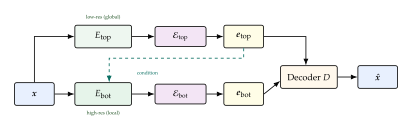
A top-level encoder $E_{top}$ that produces a low-resolution latent map quantised with codebook $ℰ_{top}$ , capturing global structure.
A bottom-level encoder $E_{bot}$ that produces a higher-resolution latent map quantised with codebook $ℰ_{bot}$ , conditioned on the top-level codes, capturing local detail.
A decoder $D$ that reconstructs the input from both levels: $\hat{𝒙} = D (𝒆_{top}, 𝒆_{bot})$ .

For example, a $256 \times 256$ image might be encoded to a $32 \times 32$ top-level map and a $64 \times 64$ bottom-level map.

Stage 1: Hierarchical Encoding and Reconstruction

The first training stage learns the hierarchical codebooks and the decoder jointly, using the standard VQ-VAE loss applied to both levels.

Algorithm 1 (VQ-VAE-2 Stage 1: Codebook Training).

Input: Encoders $E_{top}, E_{bot}$ ; decoder $D$ ; codebooks $ℰ_{top}, ℰ_{bot}$ ; training batch $𝒙$
$h_{top} \leftarrow E_{top} (𝒙)$ Encode at low resolution
$𝒆_{top} \leftarrow Quantise (h_{top}, ℰ_{top})$ Nearest-neighbour lookup in top codebook
$h_{bot} \leftarrow E_{bot} (𝒙, 𝒆_{top})$ Encode at high resolution, conditioned on top codes
$𝒆_{bot} \leftarrow Quantise (h_{bot}, ℰ_{bot})$ Nearest-neighbour lookup in bottom codebook
$\hat{𝒙} \leftarrow D (𝒆_{top}, 𝒆_{bot})$ Decode from both levels
Update all parameters via $\nabla L (𝒙, \hat{𝒙})$ VQ-VAE loss at both levels

Stage 2: Autoregressive Prior over Codes

Once the codebooks are trained, the second stage fits an autoregressive prior over the discrete codes. This decouples representation learning (stage 1) from density modelling (stage 2).

Algorithm 2 (VQ-VAE-2 Stage 2: Prior Training and Sampling).

Input: Frozen encoders $E_{top}, E_{bot}$ and codebooks from Stage 1
$T_{top}, T_{bot} \leftarrow \emptyset$ Collect code datasets
for each $𝒙$ in training set
$𝒆_{top} \leftarrow Quantise (E_{top} (𝒙), ℰ_{top})$
$𝒆_{bot} \leftarrow Quantise (E_{bot} (𝒙, 𝒆_{top}), ℰ_{bot})$
$T_{top} \leftarrow T_{top} \cup {𝒆_{top}}$ ; $T_{bot} \leftarrow T_{bot} \cup {𝒆_{bot}}$
$p_{top} \leftarrow TrainPixelCNN (T_{top})$ Unconditional autoregressive prior
$p_{bot} \leftarrow TrainCondPixelCNN (T_{bot}, T_{top})$ Conditional on top codes
Sampling:
$𝒆_{top} \sim p_{top}$ Sample top codes autoregressively
$𝒆_{bot} \sim p_{bot} (\cdot | 𝒆_{top})$ Sample bottom codes conditioned on top
$\hat{𝒙} \leftarrow D (𝒆_{top}, 𝒆_{bot})$ Decode to image

Remark 5 (Why Two Stages?).

Stage 1 learns the codebook (compression), while stage 2 learns the prior over codes (generation). This separation simplifies training considerably: the VQ-VAE objective in stage 1 does not require modelling the full joint distribution of codes, and the autoregressive model in stage 2 operates over a much smaller, discrete space rather than raw pixels.

Remark 6 (Codebook Collapse).

A practical challenge in VQ-VAE training is codebook collapse: some codebook vectors are never selected as nearest neighbours and therefore receive no gradient updates. Over time, these “dead” vectors drift further from the encoder outputs and are never used again. A common mitigation is random restarts: periodically reassign dead codebook vectors to randomly chosen encoder outputs, ensuring all vectors remain in active use.

VQ-VAE-2 hierarchical architecture. The top-level encoder captures global structure at low resolution; the bottom-level encoder captures local detail at higher resolution, conditioned on the top-level codes. The decoder reconstructs from both levels.

Historical Note.

Ali Razavi, Aaron van den Oord, and Oriol Vinyals published VQ-VAE-2 at NeurIPS 2019 [7]. The paper showed that a two-stage pipeline, separating representation learning from density modelling, could generate diverse $256 \times 256$ images that rivalled the quality of BigGAN. The key architectural insight was that hierarchical codebooks allow the model to allocate capacity efficiently: the top level handles global composition while the bottom level handles textures and fine details.

Case Study: High-Fidelity Image Generation with VQ-VAE-2

How well can a likelihood-based model compete with GANs on image quality? Before VQ-VAE-2, the conventional wisdom was that GANs produced sharp images while VAEs produced blurry ones. Razavi et al. [7] challenged this assumption head-on.

Architecture Details

For $256 \times 256$ ImageNet generation, VQ-VAE-2 uses the two-level hierarchy described in Definition 9:

Level	Resolution	Downsample	Codebook $K$	Dim $d$	Captures
Top	$32 \times 32$	$8 \times$ from input	512	64	global structure
Bottom	$64 \times 64$	$4 \times$ from input	512	64	local detail

The encoder and decoder are built from residual blocks with $128$ hidden units and $3 \times 3$ convolutions. Strided convolutions handle downsampling in the encoder, and strided transposed convolutions handle upsampling in the decoder. The codebook uses exponential moving average (EMA) updates with decay $γ = 0.99$ and commitment loss coefficient $β = 0.25$ .

The total compression ratio is striking: a $256 \times 256 \times 3$ image ( $196,608$ values) is compressed to $32 \times 32 + 64 \times 64 = 5,120$ discrete codes, a roughly $𝟑𝟖 \times$ compression. For $1024 \times 1024$ face generation on FFHQ, a three-level hierarchy achieves approximately $200 \times$ compression.

The PixelSNAIL Prior

The Stage 2 autoregressive priors are powerful models in their own right:

Top prior ( $32 \times 32$ codes): a gated PixelCNN with multi-headed self-attention (PixelSNAIL-style), using $20$ layers, $512$ hidden units, and $4$ attention layers with $8$ heads each. Self-attention at $32 \times 32$ resolution is tractable and allows the prior to capture long-range spatial dependencies across the entire image.
Bottom prior ( $64 \times 64$ codes): a deep conditional PixelCNN without self-attention (since attention over $64 \times 64 = 4,096$ positions is prohibitively expensive). Instead, global context is provided by conditioning on the top-level codes through a $20$ -layer residual conditioning stack.

Remark 7 (Classifier-Based Rejection Sampling).

To improve sample quality further, the authors introduce a rejection sampling scheme: generate candidate images from the prior, score each with a pretrained ImageNet classifier, and reject samples where the classifier's confidence in the target class falls below a threshold. This provides a smooth quality-diversity trade-off, analogous to the truncation trick in BigGAN. Stricter rejection produces higher-fidelity but less diverse samples.

Results: Rivalling GANs

The results challenged the prevailing belief that likelihood-based models could not match GAN quality. To measure both quality and diversity, the authors used the Classification Accuracy Score (CAS): train an ImageNet classifier exclusively on generated samples, then evaluate it on real test images. A model suffering from mode collapse produces a poor classifier, regardless of individual sample quality.

Model	CAS Top-1 (%)	CAS Top-5 (%)
VQ-VAE-2	$𝟓𝟒.𝟖𝟑$	$𝟕𝟕.𝟓𝟗$
BigGAN-deep (truncation $1.0$ )	$42.65$	$65.92$
Real data (upper bound)	$73.09$	$91.47$

VQ-VAE-2 significantly outperforms BigGAN on diversity (CAS), while producing images that are visually competitive in quality. The precision-recall analysis confirmed this: VQ-VAE-2 achieves slightly lower precision (individual sample sharpness) but substantially higher recall (mode coverage) than BigGAN.

Insight.

VQ-VAE-2 demonstrated a crucial lesson for generative modelling: sample quality and sample diversity are distinct goals, and models should be evaluated on both. A model that produces stunning samples of only a few modes (like a mode-collapsing GAN) may look impressive on FID but fail on diversity-sensitive metrics like CAS.

Case Study: Jukebox and Music Generation

Can the VQ-VAE framework extend beyond images to generate minutes of coherent music with singing? Jukebox [8], developed at OpenAI, demonstrated exactly this by scaling hierarchical VQ-VAE to raw audio. The challenge is immense: a four-minute song at $44.1 kHz$ contains over $10$ million samples, orders of magnitude more than a $256 \times 256$ image.

Three-Level VQ-VAE for Audio

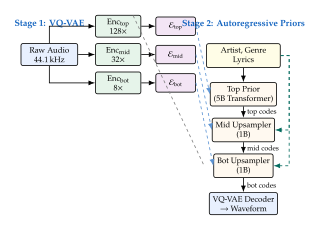
Jukebox uses three independently trained VQ-VAE levels, each compressing raw audio at a different temporal resolution:

Level	Hop Length	Compression	Codebook $K$	Context ( $\sim$ seconds)
Bottom	$8$	$8 \times$	$2048$	$\sim 1.5$
Middle	$32$	$32 \times$	$2048$	$\sim 6$
Top	$128$	$128 \times$	$2048$	$\sim 24$

Each encoder uses downsampling convolutions followed by residual blocks of non-causal 1-D dilated convolutions (WaveNet-style, dilation growth rate $3$ , filter size $3$ ). The decoder mirrors this structure. The entire VQ-VAE has only about $2$ million parameters, a tiny fraction of the overall system.

The hierarchy creates a natural separation of information: the top level, which compresses $128$ audio samples into a single code, captures high-level musical structure (melody, rhythm, song sections). The bottom level, at $8 \times$ compression, captures fine acoustic detail (timbre, consonants, breaths).

Jukebox architecture overview. Stage 1 (left): three independently trained VQ-VAE levels compress raw

44.1 kHz

audio at

8 \times

32 \times

, and

128 \times

compression, each with a codebook of

2,048

entries. Stage 2 (right): autoregressive sparse transformers generate codes top-down, conditioned on artist, genre, and lyrics. The VQ-VAE decoder converts the generated codes back to a waveform.

Combating Codebook Collapse with Random Restarts

With $2,048$ codebook entries per level, maintaining full codebook utilisation is critical. Jukebox tracks the mean usage of each codebook vector via an exponential moving average. When usage falls below a threshold, the “dead” vector is randomly reset to one of the encoder outputs from the current batch. This simple strategy maintains approximately $11$ bits of codebook entropy (the maximum for $K = 2,048$ ) throughout training, confirming near-complete utilisation.

Spectral Loss for Audio Fidelity

A standard sample-level $L_{2}$ reconstruction loss tends to reconstruct only low frequencies, producing muffled audio. Jukebox addresses this with a multi-scale spectral loss, computed on magnitude spectrograms at three resolutions: (Spectral LOSS) $\begin{matrix} L_{spec} = \sum_{s \in 𝒮} ‖ | {STFT}_{s} (𝒙) | - | {STFT}_{s} (\hat{𝒙}) | ‖_{2}, \end{matrix}$ where $𝒮$ indexes three STFT configurations with window sizes $1,200$ , $600$ , and $240$ samples. Operating on magnitude spectrograms (ignoring phase) captures frequency content across multiple time scales.

The total VQ-VAE loss combines all components: (Jukebox Vqvae LOSS) $\begin{matrix} L = L_{recon} + L_{codebook} + β L_{commit} + L_{spec}, \end{matrix}$ with commitment coefficient $β = 0.02$ (lower than the typical $0.25$ used in image VQ-VAEs, reflecting the different loss scales in audio).

Autoregressive Priors with Sparse Transformers

The Stage 2 priors are the computational heart of Jukebox. The top-level prior is a massive $5$ billion parameter sparse transformer with $72$ layers, a width of $4,800$ dimensions, and a context window of $8,192$ tokens (about $24$ seconds of music). Full self-attention over $8,192$ tokens would be prohibitively expensive, so Jukebox uses factorised sparse attention: the token sequence is reshaped into $128 \times 64$ blocks, and three attention patterns alternate across layers:

Row attention (local context): each token attends only to tokens in the same row.
Column attention (global context): each token attends along its column across all rows.
Previous-row attention: full attention to the entire preceding row.

This factorisation reduces the attention cost from $O (n^{2})$ to $O (n \sqrt{n})$ , making it feasible to model long musical sequences.

The middle and bottom upsamplers are smaller ( $\sim 1$ billion parameters combined). They condition on the upper-level codes through a WaveNet-style residual network followed by upsampling strided convolutions.

Conditioning on Artist, Genre, and Lyrics

Jukebox conditions generation on rich metadata:

Artist and genre: Learned embedding vectors for $7,898$ artists and $604$ genres are summed and provided as the first token of each sequence.
Timing: A positional signal encodes total song duration, the current timestamp, and the fraction of the song elapsed, enabling the model to learn song structure (intros, verses, outros).
Lyrics: A character-level transformer encoder ( $18$ layers, $1,280$ dimensions) processes the lyrics. The top-level prior becomes an encoder-decoder model: $7$ cross-attention layers are interleaved into the $72$ -layer decoder, allowing music tokens to attend to lyric tokens.

Remark 8 (Scale of Jukebox Training).

Jukebox was trained on $1.2$ million songs. The VQ-VAE required $256$ V100 GPUs for $3$ days. The $5$ -billion-parameter top prior required $512$ V100s for $4$ weeks, with an additional $2$ weeks to fine-tune the lyrics conditioning. Generating one minute of top-level tokens takes approximately one hour; full upsampling to a waveform takes approximately eight hours. These numbers illustrate the immense computational cost of modelling raw audio at the waveform level.

Insight.

Jukebox validated the VQ-VAE paradigm far beyond images. By compressing $44.1 kHz$ audio at up to $128 \times$ , the discrete codebook reduces the sequence modelling problem to a tractable length for transformers. The three-level hierarchy is essential: without it, modelling the full $10$ million samples of a song autoregressively would be computationally infeasible. The two-stage recipe, learn to compress, then learn to generate in the compressed space, has since become the dominant paradigm across modalities.

Historical Note.

Prafulla Dhariwal, Heewoo Jun, Christine Payne, Jong Wook Kim, Alec Radford, and Ilya Sutskever at OpenAI released Jukebox in April 2020 [8], alongside thousands of non-cherry-picked generated samples. The model could generate coherent songs lasting several minutes, conditioned on artist style, genre, and even lyrics. While the generated audio was not indistinguishable from real recordings, it demonstrated a striking ability to capture musical structure, instrumentation, and vocal styles. The Jukebox codebase and pretrained models were publicly released, enabling further research into music generation with discrete latent codes.

Connections and Outlook

The variants we have studied form a progression from the standard VAE towards increasingly powerful and flexible generative models. The following table summarises their key properties:

1.2

Model	Latent	KL Term	Sample Quality	Key Application
VAE	continuous	analytical	blurry	general generation
$β$ -VAE	continuous	$β \times$ analytical	blurry	disentanglement
CVAE	continuous	analytical	blurry	conditional generation
VQ-VAE	discrete	constant $\log K$	moderate	discrete tokens
VQ-GAN	discrete	constant $\log K$	sharp	image tokenisation
VQ-VAE-2	discrete (hier.)	constant per level	sharp	high-res generation

Connection to diffusion models.

VQ-GAN codebooks serve as the compression backbone for latent diffusion models. Rather than running a diffusion process in pixel space (which is expensive at high resolution), latent diffusion first encodes images to a compact VQ-GAN latent grid, then applies diffusion in that compressed space. This is the architecture behind Stable Diffusion, one of the most widely deployed generative models.

Connection to transformers.

Discrete tokens from VQ-VAE and VQ-GAN are directly amenable to autoregressive modelling with transformers. Treat each codebook index as a “word” in a visual vocabulary, and a standard language model can generate images token by token. This paradigm underpins DALL-E, Parti, and other vision-language models.

Open directions.

Several challenges remain in the design of VAE variants:

Codebook utilisation: many entries remain unused even with random restarts. Better initialisation and training schedules are active research topics.
Scaling to higher resolution: adding more hierarchical levels introduces engineering complexity and can slow convergence.
Hybrid latent spaces: combining continuous and discrete latents in a single model could capture the benefits of both worlds.

Exercises

Exercise 1 (Conditional ELBO Derivation).

Derive the conditional ELBO from scratch. Starting from $\log p_{θ} (𝒙 | 𝒚)$ , introduce a variational distribution $q_{ϕ} (𝒛 | 𝒙, 𝒚)$ and show that $\log p_{θ} (𝒙 | 𝒚) \geq 𝔼_{q_{ϕ} (𝒛 | 𝒙, 𝒚)} [\log p_{θ} (𝒙 | 𝒛, 𝒚)] - 𝖣_{KL} (q_{ϕ} (𝒛 | 𝒙, 𝒚) ‖ p (𝒛)) .$ Identify the gap between the ELBO and the true log-likelihood, and explain under what conditions this gap equals zero.

Exercise 2 (Conditional Reparameterisation).

In a CVAE with Gaussian encoder $q_{ϕ} (𝒛 | 𝒙, 𝒚) = 𝒩 (𝝁_{ϕ} (𝒙, 𝒚), diag (𝝈_{ϕ}^{2} (𝒙, 𝒚)))$ , we write $𝒛 = 𝝁_{ϕ} (𝒙, 𝒚) + 𝝈_{ϕ} (𝒙, 𝒚) ⊙ 𝝐$ with $𝝐 \sim 𝒩 (0, I)$ . Prove that $𝒛$ follows the correct distribution. Then explain why this reparameterisation is necessary for computing gradients $\nabla_{ϕ}$ of the ELBO via backpropagation.

Exercise 3 ( $β$ -VAE Trade-off Analysis).

In the $β$ -VAE objective $ℒ_{β} = 𝔼_{q_{ϕ}} [\log p_{θ} (𝒙 | 𝒛)] - β 𝖣_{KL} (q_{ϕ} ‖ p)$ :

Show that $β = 1$ recovers the standard ELBO.
Prove that as $β \to \infty$ , the optimal encoder must satisfy $q_{ϕ} (𝒛 | 𝒙) = p (𝒛)$ (posterior collapse).
Argue informally why increasing $β$ encourages disentanglement, connecting your argument to the information bottleneck principle.

Exercise 4 (VAE vs. EM Algorithm).

Compare the VAE training procedure and the Expectation-Maximisation (EM) algorithm for fitting a latent variable model. Address the following:

How is the posterior over latent variables computed in each approach?
How are the model parameters updated?
What role does amortised inference play in VAEs but not in EM?

Exercise 5 (VQ-VAE Gradient Flow).

In VQ-VAE, the encoder output $z_{e} (𝒙)$ is mapped to the nearest codebook vector via $z_{q} (𝒙) = 𝒆_{k}$ where $k = {arg min}_{j} ‖ z_{e} (𝒙) - 𝒆_{j} ‖$ .

Explain why the gradient of the reconstruction loss cannot flow through the $arg min$ operation.
Describe how the straight-through estimator addresses this problem.
What is the role of the commitment loss $β {‖ z_{e} (𝒙) - sg [𝒆] ‖}^{2}$ ?

Exercise 6 (KL Divergence for Uniform Distributions).

Let $P = Uniform (0, θ_{1})$ and $Q = Uniform (0, θ_{2})$ with $θ_{1} < θ_{2}$ .

Compute the KL divergence $𝖣_{KL} (P ‖ Q)$ from its definition and show that it equals $\log (θ_{2} / θ_{1})$ .
Compute $𝖣_{KL} (Q ‖ P)$ . What happens and why?
Relate this to the VQ-VAE setting where the prior is uniform over $K$ codebook entries and the posterior is a point mass.

Exercise 7 (Ignoring $𝒚$ in the CVAE Encoder).

Consider a CVAE where the encoder ignores $𝒚$ , using $q_{ϕ} (𝒛 | 𝒙)$ instead of $q_{ϕ} (𝒛 | 𝒙, 𝒚)$ .

Show that the ELBO with this restricted encoder is at most as tight as the ELBO with the full encoder $q_{ϕ} (𝒛 | 𝒙, 𝒚)$ .
Give a concrete example where ignoring $𝒚$ leads to a strictly worse bound.
Under what condition on the true posterior $p_{θ} (𝒛 | 𝒙, 𝒚)$ does ignoring $𝒚$ incur no loss?

Exercise 8 (Constant KL in VQ-VAE).

In VQ-VAE, the posterior $q (𝒛 = k | 𝒙)$ is deterministic (one-hot) and the prior is $p (𝒛) = 1 / K$ (uniform).

Prove that $𝖣_{KL} (q ‖ p) = \log K$ for every input $𝒙$ .
Explain why this means the KL term drops out of the gradient with respect to the encoder parameters.
What would change if the prior were non-uniform, say $p (𝒛 = k) = π_{k}$ with $\sum_{k} π_{k} = 1$ ?

Exercise 9 (Exponential Moving Average Codebook Updates).

An alternative to gradient-based codebook learning is the exponential moving average (EMA) update. Let $n_{k}^{(t)}$ be the number of encoder outputs assigned to codebook entry $k$ at step $t$ , and let ${\overline{𝒛}}_{k}^{(t)}$ be their mean. The EMA update rule is: $\begin{matrix} N_{k}^{(t)} & = γ N_{k}^{(t - 1)} + (1 - γ) n_{k}^{(t)}, \\ m_{k}^{(t)} & = γ m_{k}^{(t - 1)} + (1 - γ) \sum_{i : q_{i} = k} z_{e} (𝒙_{i}), \\ 𝒆_{k}^{(t)} & = m_{k}^{(t)} / N_{k}^{(t)}, \end{matrix}$ where $γ \in (0, 1)$ is the decay rate.

Show that in steady state (when statistics are stationary), $𝒆_{k}$ converges to the mean of encoder outputs assigned to entry $k$ .
Compare this to the gradient-based codebook update from the loss term ${‖ sg [z_{e} (𝒙)] - 𝒆 ‖}^{2}$ . Which approach is more stable, and why?
What happens to $𝒆_{k}$ if entry $k$ receives no assignments for many consecutive steps?

Exercise 10 (Adversarial Loss and Mode Behaviour).

In VQ-GAN, the adversarial loss $L_{GAN}$ supplements the reconstruction loss ${‖ 𝒙 - \hat{𝒙} ‖}^{2}$ .

Explain why the $L_{2}$ reconstruction loss is mode-covering (it prefers blurry averages over sharp samples) while the adversarial loss is mode-seeking (it rewards sharp, realistic outputs).
Why does combining both losses yield better results than either alone?
The perceptual loss $L_{perc}$ compares features from a pretrained VGG network rather than raw pixels. Explain why this encourages structural similarity rather than pixel-level matching.

References

Auto-Encoding Variational Bayes

Diederik P Kingma, Max Welling

International Conference on Learning Representations · 2014

BibTeX

@inproceedings{kingma2013auto,
  title={Auto-Encoding Variational {B}ayes},
  author={Kingma, Diederik P and Welling, Max},
  booktitle={International Conference on Learning Representations},
  year={2014}
}

Conference paper

$eta$-VAE: Learning Basic Visual Concepts with a Constrained Variational Framework

Irina Higgins, Loic Matthey, Arka Pal, Christopher Burgess, Xavier Glorot, Matthew Botvinick, Shakir Mohamed, Alexander Lerchner

International Conference on Learning Representations · 2017

BibTeX

@inproceedings{higgins2017beta,
  title={$\beta$-{VAE}: Learning Basic Visual Concepts with a Constrained Variational Framework},
  author={Higgins, Irina and Matthey, Loic and Pal, Arka and Burgess, Christopher and Glorot, Xavier and Botvinick, Matthew and Mohamed, Shakir and Lerchner, Alexander},
  booktitle={International Conference on Learning Representations},
  year={2017}
}

Conference paper

Learning Structured Output Representation using Deep Conditional Generative Models

Kihyuk Sohn, Honglak Lee, Xinchen Yan

Advances in Neural Information Processing Systems, pp. 3483-3491 · 2015

BibTeX

@inproceedings{sohn2015cvae,
  title={Learning Structured Output Representation using Deep Conditional Generative Models},
  author={Sohn, Kihyuk and Lee, Honglak and Yan, Xinchen},
  booktitle={Advances in Neural Information Processing Systems},
  pages={3483--3491},
  year={2015}
}

Conference paper

An Algorithm for Vector Quantizer Design

Yoseph Linde, Andres Buzo, Robert M Gray

IEEE Transactions on Communications, vol. 28, no. 1, pp. 84-95 · 1980

BibTeX

@article{linde1980algorithm,
  title={An Algorithm for Vector Quantizer Design},
  author={Linde, Yoseph and Buzo, Andr{\'e}s and Gray, Robert M},
  journal={IEEE Transactions on Communications},
  volume={28},
  number={1},
  pages={84--95},
  year={1980}
}

Journal article

Neural Discrete Representation Learning

Aaron van den Oord, Oriol Vinyals, Koray Kavukcuoglu

Advances in Neural Information Processing Systems, pp. 6306-6315 · 2017

BibTeX

@inproceedings{oord2017vqvae,
  title={Neural Discrete Representation Learning},
  author={van den Oord, Aaron and Vinyals, Oriol and Kavukcuoglu, Koray},
  booktitle={Advances in Neural Information Processing Systems},
  pages={6306--6315},
  year={2017}
}

Conference paper

Taming Transformers for High-Resolution Image Synthesis

Patrick Esser, Robin Rombach, Bjorn Ommer

Proceedings of the IEEE/CVF Conference on Computer Vision and Pattern Recognition, pp. 12873-12883 · 2021

BibTeX

@inproceedings{esser2021vqgan,
  title={Taming Transformers for High-Resolution Image Synthesis},
  author={Esser, Patrick and Rombach, Robin and Ommer, Bj{\"o}rn},
  booktitle={Proceedings of the IEEE/CVF Conference on Computer Vision and Pattern Recognition},
  pages={12873--12883},
  year={2021}
}

Conference paper

Generating Diverse High-Fidelity Images with VQ-VAE-2

Ali Razavi, Aaron van den Oord, Oriol Vinyals

Advances in Neural Information Processing Systems, pp. 14866-14876 · 2019

BibTeX

@inproceedings{razavi2019vqvae2,
  title={Generating Diverse High-Fidelity Images with {VQ-VAE-2}},
  author={Razavi, Ali and van den Oord, Aaron and Vinyals, Oriol},
  booktitle={Advances in Neural Information Processing Systems},
  pages={14866--14876},
  year={2019}
}

Conference paper

Jukebox: A Generative Model for Music

Prafulla Dhariwal, Heewoo Jun, Christine Payne, Jong Wook Kim, Alec Radford, Ilya Sutskever

arXiv preprint arXiv:2005.00341 · 2020

BibTeX

@article{dhariwal2020jukebox,
  title={Jukebox: A Generative Model for Music},
  author={Dhariwal, Prafulla and Jun, Heewoo and Payne, Christine and Kim, Jong Wook and Radford, Alec and Sutskever, Ilya},
  journal={arXiv preprint arXiv:2005.00341},
  year={2020}
}

Journal article

← 15 Variational Autoencoders 17 Autoregressive Models →

16 Advanced VAE Variants

From VAEs to VAE Variants

The β-VAE: Disentangled Representations

Conditional VAE

From Continuous to Discrete Latent Spaces

VQ-VAE: Vector Quantised Variational Autoencoder

Architecture

Posterior and KL Divergence

The VQ-VAE Loss Function

Gradient Flow: The Straight-Through Estimator

VQ-GAN: Adversarial Codebook Learning

VQ-VAE-2: Hierarchical Discrete Representations

Stage 1: Hierarchical Encoding and Reconstruction

Stage 2: Autoregressive Prior over Codes

Case Study: High-Fidelity Image Generation with VQ-VAE-2

Architecture Details

The PixelSNAIL Prior

Results: Rivalling GANs

Case Study: Jukebox and Music Generation

Three-Level VQ-VAE for Audio

Combating Codebook Collapse with Random Restarts

Spectral Loss for Audio Fidelity

Autoregressive Priors with Sparse Transformers

Conditioning on Artist, Genre, and Lyrics

Connections and Outlook

Connection to diffusion models.

Connection to transformers.

Open directions.

Exercises

References

The $β$ -VAE: Disentangled Representations