17 Autoregressive Models

Every probability distribution over a high-dimensional space can be decomposed, exactly and without any approximation, into a product of one-dimensional conditionals. This simple observation, the probability chain rule, is the foundation of autoregressive models, a family of generative models that parameterise each conditional with a neural network and generate data one component at a time.

This chapter traces the idea from classical $n$ -gram language models through a sequence of increasingly powerful neural architectures:

We begin with the chain rule and the autoregressive factorisation of a joint distribution.
We revisit $n$ -gram language models, the earliest practical autoregressive models, together with smoothing techniques and the notion of perplexity.
We introduce Fully-Visible Sigmoid Belief Networks (FVSBNs), the first neural autoregressive models.
We develop NADE (Neural Autoregressive Density Estimation), which shares parameters across conditionals.
We present MADE (Masked Autoencoder for Distribution Estimation), which enforces autoregressive structure through masking.
We move to images with PixelRNN and the Row LSTM.
We study PixelCNN and the Gated PixelCNN, which replace recurrence with masked convolutions.
We discuss WaveNet and dilated causal convolutions for audio generation.
We examine training autoregressive models: teacher forcing, exposure bias, and scheduled sampling.
We survey modern developments: PixelSNAIL, ImageGPT, and VAR.

Historical Note.

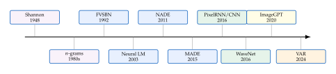
The idea of modelling sequences by conditioning each element on its predecessors dates back at least to Andrei Markov, who in 1906 studied the alternation of vowels and consonants in Pushkin's Eugene Onegin [1]. Claude Shannon's 1948 landmark paper formalised language as a stochastic process and used $n$ -gram statistics to generate English text, famously demonstrating that longer contexts improve text quality [1][2]. The neural revolution arrived with Bengio et al.'s 2003 neural language model [3], followed by NADE [4] and MADE [5] for density estimation, PixelRNN/CNN [6] and WaveNet [7] for images and audio, and ultimately the Transformer, which powers today's large language models.

The Chain Rule and Autoregressive Factorisation

Let $𝒙 = (x_{1}, x_{2}, \dots, x_{D}) \in 𝒳^{D}$ be a $D$ -dimensional random vector with joint density $p (𝒙)$ . The probability chain rule gives an exact factorisation of the joint into a product of conditionals:

Definition 1 (Autoregressive Factorisation).

The autoregressive factorisation of a joint density $p (𝒙)$ is (Chain RULE) $\begin{matrix} p (𝒙) = \prod_{d = 1}^{D} p (x_{d} | x_{1}, \dots, x_{d - 1}) = \prod_{d = 1}^{D} p (x_{d} | 𝒙_{< d}), \end{matrix}$ where $𝒙_{< d} = (x_{1}, \dots, x_{d - 1})$ denotes the context of dimension $d$ , with the convention that $𝒙_{< 1} = \emptyset$ so that the first factor is the marginal $p (x_{1})$ .

This factorisation holds for any ordering of the dimensions and for any distribution, discrete or continuous, simple or complex. No modelling assumptions have been made.

Remark 1 (Ordering matters in practice).

Although the chain rule is valid for every permutation of $(1,2, \dots, D)$ , different orderings may lead to conditionals of very different complexity. For text, the left-to-right reading order is natural; for images, the raster-scan order (left-to-right, top-to-bottom) has become standard [6].

Directed acyclic graph for the autoregressive factorisation. Each variable

x_{d}

depends on all preceding variables

x_{1}, \dots, x_{d - 1}

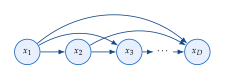
An autoregressive model parameterises each conditional $p (x_{d} | 𝒙_{< d})$ with a learnable function, for example, a neural network with parameters $θ$ . Writing $p_{θ} (x_{d} | 𝒙_{< d})$ for each conditional, the model density is (Model Density) $\begin{matrix} p_{θ} (𝒙) = \prod_{d = 1}^{D} p_{θ} (x_{d} | 𝒙_{< d}) . \end{matrix}$ Because each factor is a valid conditional distribution (it integrates or sums to one), the product is automatically a valid joint distribution, regardless of the choice of parameters $θ$ . This is a major advantage over energy-based models, which require a normalising constant that is generally intractable.

Training by maximum likelihood.

Given a dataset $𝒟 = {𝒙^{(1)}, \dots, 𝒙^{(N)}}$ , training proceeds by maximising the log-likelihood: (NLL) $\begin{matrix} ℓ (θ) = \frac{1}{N} \sum_{n = 1}^{N} \log p_{θ} (𝒙^{(n)}) = \frac{1}{N} \sum_{n = 1}^{N} \sum_{d = 1}^{D} \log p_{θ} (x_{d}^{(n)} | 𝒙_{< d}^{(n)}) . \end{matrix}$ Each term in the inner sum can be computed in parallel during training, because the conditioning context $𝒙_{< d}^{(n)}$ is observed, so we simply plug in the true data. This is known as teacher forcing and will be discussed in detail in Training Autoregressive Models.

Generation.

Sampling from an autoregressive model is inherently sequential: we first draw $x_{1} \sim p_{θ} (x_{1})$ , then $x_{2} \sim p_{θ} (x_{2} | x_{1})$ , and so on. This sequential nature is the main computational bottleneck of autoregressive models.

Key Idea.

Autoregressive models are exact: no variational approximation, no adversarial training, no intractable normalising constant. The chain rule guarantees a valid density, and log-likelihoods can be computed exactly. The price is slow generation, because sampling requires $D$ sequential steps.

$N$ -gram Language Models

The autoregressive factorisation is at the heart of language modelling: given a sequence of words $w_{1}, w_{2}, \dots, w_{T}$ from a vocabulary $𝒱$ of size $V$ , we model the joint probability as $p (w_{1}, \dots, w_{T}) = \prod_{t = 1}^{T} p (w_{t} | w_{1}, \dots, w_{t - 1}) .$ The challenge is that the conditioning context grows with $t$ , so the number of parameters needed to represent each conditional exactly grows exponentially. The classical solution is to truncate the context.

Definition 2 ( $N$ -gram model).

An $N$ -gram model (or $(N - 1)$ th-order Markov model) assumes that the probability of a word depends only on the preceding $N - 1$ words: (Ngram) $\begin{matrix} p (w_{t} | w_{1}, \dots, w_{t - 1}) \approx p (w_{t} | w_{t - N + 1}, \dots, w_{t - 1}) . \end{matrix}$ The conditional probabilities are estimated by counting $N$ -grams in a training corpus: (Ngram MLE) $\begin{matrix} \hat{p} (w_{t} | w_{t - N + 1}, \dots, w_{t - 1}) = \frac{count (w_{t - N + 1}, \dots, w_{t})}{count (w_{t - N + 1}, \dots, w_{t - 1})} . \end{matrix}$

Example 1 (Bigram model).

A bigram model ( $N = 2$ ) estimates each word probability from only the immediately preceding word: $p (w_{t} | w_{t - 1}) = \frac{count (w_{t - 1}, w_{t})}{count (w_{t - 1})} .$ Consider the sentence “the cat sat on the mat” with a vocabulary $𝒱 = {the, cat, sat, on, mat}$ . From this single training sentence we obtain: $p (cat | the) = \frac{1}{2}, p (mat | the) = \frac{1}{2}, p (sat | cat) = 1, p (on | sat) = 1.$ The bigram $(the, sat)$ has count zero, so the MLE assigns $p (sat | the) = 0$ . This zero-probability problem motivates the smoothing techniques discussed below.

The sparsity problem

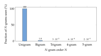
As $N$ grows, the number of distinct $N$ -grams is $V^{N}$ , but a finite corpus can only contain a tiny fraction of them. Most $N$ -grams will have zero counts, and the MLE will assign zero probability to any sequence containing an unseen $N$ -gram.

Illustrative fraction of possible

N

-grams observed in a typical English corpus with

V = 50,000

. Even at

N = 2

, most bigrams never appear; by

N = 5

, the observed fraction is negligible. The figures indicate the trend only: they are not mutually consistent for a single corpus, since the implied number of distinct observed

N

-grams varies by many orders of magnitude across the bars.

Smoothing techniques

To avoid zero probabilities, we modify the count-based estimates through smoothing.

Definition 3 (Laplace (add- $α$ ) smoothing).

Laplace smoothing adds a pseudo-count $α > 0$ to every $N$ -gram: (Laplace) $\begin{matrix} {\hat{p}}_{α} (w_{t} | w_{t - N + 1}, \dots, w_{t - 1}) = \frac{count (w_{t - N + 1}, \dots, w_{t}) + α}{count (w_{t - N + 1}, \dots, w_{t - 1}) + α V} . \end{matrix}$

Laplace smoothing is simple but crude: it steals too much probability mass from frequent $N$ -grams. More sophisticated methods include:

Interpolation: combine estimates from different orders by a weighted average: (Interpolation) $\begin{matrix} \hat{p} (w_{t} | w_{t - 2}, w_{t - 1}) = λ_{3} {\hat{p}}_{3} (w_{t} | w_{t - 2}, w_{t - 1}) + λ_{2} {\hat{p}}_{2} (w_{t} | w_{t - 1}) + λ_{1} {\hat{p}}_{1} (w_{t}), \end{matrix}$ where $λ_{1} + λ_{2} + λ_{3} = 1$ and the weights are tuned on held-out data.
Backoff (Katz): use the highest-order estimate when it is reliable, and back off to lower-order estimates otherwise.
Kneser–Ney smoothing: uses the number of distinct contexts in which a word appears, rather than raw counts, leading to better estimates for rare words.

Perplexity

How do we compare language models? The standard metric is perplexity, which measures how “surprised” the model is by held-out text.

Definition 4 (Perplexity).

The perplexity of a model $p$ on a test sequence $w_{1}, \dots, w_{T}$ is (PPL) $\begin{matrix} PPL (p) = p (w_{1}, \dots, w_{T})^{- 1 / T} = \exp (- \frac{1}{T} \sum_{t = 1}^{T} \log p (w_{t} | w_{< t})) . \end{matrix}$

A lower perplexity indicates a better model. Intuitively, a perplexity of $k$ means the model is as uncertain as if it were choosing uniformly among $k$ words at each step.

Proposition 1 (Perplexity and cross-entropy).

Let $p_{data}$ denote the true distribution of the language and $p_{θ}$ the model. As $T \to \infty$ , the per-word log-likelihood converges (under ergodicity) to the negative cross-entropy: $- \frac{1}{T} \sum_{t = 1}^{T} \log p_{θ} (w_{t} | w_{< t}) \overset{\overset{}{T \to \infty}}{\to} 𝖧 (p_{data}, p_{θ}) = 𝔼_{p_{data}} [- \log p_{θ} (w_{t} | w_{< t})],$ the cross-entropy rate of the model with respect to the source. (The quantity that converges is the average conditional log-loss, so the limit is a rate, not the marginal sum $- \sum_{w} p_{data} (w) \log p_{θ} (w)$ ; the two coincide only when the source is memoryless.) Therefore $PPL (p_{θ}) \to \exp (𝖧 (p_{data}, p_{θ}))$ , and minimising perplexity is equivalent to minimising the cross-entropy (or equivalently the KL divergence $𝖣_{KL} (p_{data} ‖ p_{θ})$ ).

Proof.

By the Shannon–McMillan–Breiman theorem, for a stationary ergodic source, $- \frac{1}{T} \log p_{data} (w_{1}, \dots, w_{T}) \overset{\overset{}{T \to \infty}}{\to} 𝖧 (p_{data}) .$ The model's per-word log-loss on data drawn from $p_{data}$ converges to $𝔼_{p_{data}} [- \log p_{θ} (w_{t} | w_{< t})] = 𝖧 (p_{data}, p_{θ}) .$ Since $𝖧 (p_{data}, p_{θ}) = 𝖧 (p_{data}) + 𝖣_{KL} (p_{data} ‖ p_{θ})$ , minimising cross-entropy is equivalent to minimising the KL divergence. Exponentiating gives the perplexity result.

∎

Historical Note.

Fred Jelinek and his team at IBM pioneered the use of $n$ -gram models and perplexity for speech recognition in the 1970s and 1980s. Jelinek reportedly quipped, “Every time I fire a linguist, the performance of the speech recogniser goes up.” Shannon himself estimated the entropy of English at about 1.0–1.3 bits per character in 1951 [2], a figure that has held up remarkably well.

Fully-Visible Sigmoid Belief Networks

The earliest neural autoregressive model was proposed by Neal [11] in 1992. Rather than using $n$ -gram counts, the idea is to parameterise each conditional $p (x_{d} | 𝒙_{< d})$ with a logistic regression.

Definition 5 (Fully-Visible Sigmoid Belief Network).

Let $𝒙 \in {0,1}^{D}$ be a binary vector. A Fully-Visible Sigmoid Belief Network (FVSBN) models each conditional as (Fvsbn) $\begin{matrix} p (x_{d} = 1 | 𝒙_{< d}) = σ (𝒘_{d}^{⊤} 𝒙_{< d} + b_{d}), \end{matrix}$ where $σ (a) = 1 / (1 + e^{- a})$ is the sigmoid function, $𝒘_{d} \in ℝ^{d - 1}$ is a weight vector, and $b_{d} \in ℝ$ is a bias. Each conditional uses its own parameters $(𝒘_{d}, b_{d})$ .

The FVSBN is a valid autoregressive model: $p (x_{d} | 𝒙_{< d})$ depends only on dimensions $1, \dots, d - 1$ , and the sigmoid ensures the output is a valid probability. The total number of parameters is $\sum_{d = 1}^{D} d = D (D + 1) / 2$ , which is quadratic in $D$ .

Insight.

The FVSBN is essentially a logistic regression for each conditional. Its expressiveness is limited because each conditional is a linear function of the context, passed through a sigmoid. This means the model cannot capture nonlinear interactions between preceding dimensions. NADE, introduced next, overcomes this limitation by adding a hidden layer with shared weights.

NADE: Neural Autoregressive Density Estimation

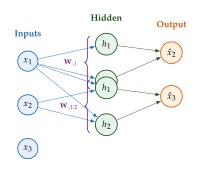
NADE (Neural Autoregressive Density Estimator), introduced by Larochelle and Murray [4], replaces each logistic regression in the FVSBN with a one-hidden-layer neural network whose weights are shared across all conditionals.

Definition 6 (NADE).

For binary data $𝒙 \in {0,1}^{D}$ , NADE computes each conditional as follows. For $d = 1, 2, \dots, D$ : (NADE Hidden) $\begin{matrix} 𝒉_{d} & = σ (𝐖_{:, < d} 𝒙_{< d} + 𝒄), \\ p (x_{d} = 1 | 𝒙_{< d}) & = σ (𝐕_{d, :} 𝒉_{d} + b_{d}), \end{matrix}$ where $𝐖 \in ℝ^{H \times D}$ is a shared weight matrix (with $𝐖_{:, < d}$ denoting its first $d - 1$ columns), $𝒄 \in ℝ^{H}$ is a shared bias, $𝐕 \in ℝ^{D \times H}$ contains the output weights, $b_{d} \in ℝ$ is an output bias, and $H$ is the number of hidden units.

NADE architecture for

D = 3

with

H = 2

hidden units. The weight matrix

𝐖

is shared across conditionals: predicting

x_{2}

uses column 1 of

𝐖

, predicting

x_{3}

uses columns 1 and 2. This sharing is the key difference from FVSBN, which uses separate parameters for each conditional.

Proposition 2 (Efficient computation via weight sharing).

The hidden activations $𝒉_{d}$ in NADE satisfy the recurrence (NADE Recurrence) $\begin{matrix} 𝒂_{d} = 𝒂_{d - 1} + 𝐖_{:, d - 1} x_{d - 1}, 𝒉_{d} = σ (𝒂_{d}), \end{matrix}$ with $𝒂_{1} = 𝒄$ . Therefore all $D$ conditionals can be computed in $𝒪 (D H)$ time, the same cost as a single forward pass through a network with $H$ hidden units.

Proof.

By definition, $𝒂_{d} = 𝐖_{:, < d} 𝒙_{< d} + 𝒄$ . We can write $𝒂_{d} = \sum_{j = 1}^{d - 1} 𝐖_{:, j} x_{j} + 𝒄 = \underset{𝒂_{d - 1}}{\underset{⏟}{(\sum_{j = 1}^{d - 2} 𝐖_{:, j} x_{j} + 𝒄)}} + 𝐖_{:, d - 1} x_{d - 1},$ which gives the recurrence. Each step costs $𝒪 (H)$ (one column-vector addition plus an element-wise sigmoid), so all $D$ steps together cost $𝒪 (D H)$ .

∎

Algorithm 1 (NADE forward pass).

Input: Input $𝒙 \in {0,1}^{D}$ , parameters $𝐖 \in ℝ^{H \times D}$ , $𝐕 \in ℝ^{D \times H}$ , $𝒄 \in ℝ^{H}$ , $𝒃 \in ℝ^{D}$
Output: Log-likelihood $ℓ = \log p (𝒙)$
$𝒂 \leftarrow 𝒄$ Pre-activation initialised to bias
$ℓ \leftarrow 0$
for $d = 1, 2, \dots, D$
$𝒉 \leftarrow σ (𝒂)$ Hidden activation
${\hat{p}}_{d} \leftarrow σ (𝐕_{d, :} 𝒉 + b_{d})$ Conditional probability
$ℓ \leftarrow ℓ + x_{d} \log {\hat{p}}_{d} + (1 - x_{d}) \log (1 - {\hat{p}}_{d})$
$𝒂 \leftarrow 𝒂 + 𝐖_{:, d} x_{d}$ Incremental update
return $ℓ$

Deep NADE.

Uria et al. [12] extended NADE to multiple hidden layers, resulting in Deep NADE. Each conditional uses the same architecture, with multiple hidden layers with shared weights and the same incremental computation trick. Deep NADE achieved state-of-the-art density estimation results on binarised MNIST at the time of publication.

NADE for continuous data.

For continuous data, the output distribution can be replaced with a mixture of Gaussians: (NADE MOG) $\begin{matrix} p (x_{d} | 𝒙_{< d}) = \sum_{k = 1}^{K} π_{d, k} 𝒩 (x_{d}; μ_{d, k}, σ_{d, k}^{2}), \end{matrix}$ where the mixture weights $π_{d, k}$ , means $μ_{d, k}$ , and variances $σ_{d, k}^{2}$ are all functions of the hidden state $𝒉_{d}$ . This variant is called RNADE [13].

MADE: Masked Autoencoders for Distribution Estimation

NADE achieves efficient density estimation but uses a specialised architecture. Germain et al. [5] showed that any standard feedforward autoencoder can be turned into an autoregressive model by simply masking its weight matrices to enforce the autoregressive property.

Definition 7 (MADE).

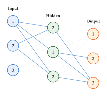
A Masked Autoencoder for Distribution Estimation (MADE) is a feedforward autoencoder whose weight matrices are element-wise multiplied by binary masks $𝐌^{(ℓ)}$ that ensure each output ${\hat{x}}_{d}$ depends only on $𝒙_{< d}$ : (MADE MASK) $\begin{matrix} \hat{𝒙} = f ((𝐖^{(L)} ⊙ 𝐌^{(L)}) \dots σ ((𝐖^{(1)} ⊙ 𝐌^{(1)}) 𝒙 + 𝒃^{(1)}) \dots + 𝒃^{(L)}), \end{matrix}$ where $⊙$ denotes element-wise multiplication and $𝐌^{(ℓ)} \in {0,1}^{n_{ℓ} \times n_{ℓ - 1}}$ are the masks.

Constructing the masks.

The masking scheme works as follows:

Assign each unit in the network a “connectivity number” $m (k)$ . Input units are assigned $m (k) = k$ for $k = 1, \dots, D$ . Hidden units are assigned numbers drawn uniformly from ${1, \dots, D - 1}$ . Output unit $d$ has connectivity number $m (d) = d$ .
The mask for layer $ℓ$ is defined by (MADE MASK RULE) $\begin{matrix} M_{k, k^{'}}^{(ℓ)} = {\begin{matrix} 𝟙 {m^{(ℓ)} (k) \geq m^{(ℓ - 1)} (k^{'})} & for hidden layers, \\ 𝟙 {m^{(L)} (k) > m^{(L - 1)} (k^{'})} & for the output layer, \end{matrix} \end{matrix}$ where the strict inequality for the output layer ensures that ${\hat{x}}_{d}$ does not depend on $x_{d}$ itself.

MADE masking for

D = 3

with one hidden layer of 3 units. Numbers inside nodes are connectivity numbers. Solid lines are active connections; dashed lines are masked (zeroed) connections. Output 1 receives no input (it models

p (x_{1})

), output 2 depends only on

x_{1}

, and output 3 depends on

x_{1}

and

x_{2}

Proposition 3 (MADE satisfies the autoregressive property).

Under the masking scheme of (MADE MASK RULE), output ${\hat{x}}_{d}$ is a function of $𝒙_{< d} = (x_{1}, \dots, x_{d - 1})$ only.

Proof.

We prove by induction on layers. After layer $ℓ$ , hidden unit $k$ at layer $ℓ$ can depend only on inputs ${x_{j} : m^{(0)} (j) \leq m^{(ℓ)} (k)}$ . For the output layer, the strict inequality $m^{(L)} (d) > m^{(L - 1)} (k^{'})$ ensures that unit $d$ at the output receives information only from hidden units whose connectivity number is strictly less than $d$ , which in turn can depend only on inputs $x_{1}, \dots, x_{d - 1}$ . Therefore output $d$ depends only on $𝒙_{< d}$ .

∎

Key Idea.

MADE turns any off-the-shelf autoencoder into an autoregressive density estimator by multiplying weight matrices with binary masks. This allows using standard deep learning infrastructure (batch normalisation, dropout, residual connections) without modification. A single forward pass through the masked network computes all $D$ conditionals simultaneously.

Order agnosticism.

A powerful extension is to train MADE with different random orderings of the input dimensions at each minibatch. By randomising the connectivity numbers (and hence the masks), the model learns to predict $x_{d}$ from any subset of other dimensions, yielding an order-agnostic density estimator.

PixelRNN

We now move from generic density estimation to image generation. Van den Oord et al. [6] proposed PixelRNN and PixelCNN, applying the autoregressive principle to model images pixel by pixel.

Definition 8 (Raster-scan ordering).

For an image of height $H$ and width $W$ with $C$ colour channels, we define an ordering over all $D = H \times W \times C$ subpixels by scanning left-to-right, top-to-bottom (the raster-scan order). Within each pixel position, we order the channels as R, G, B.

Raster-scan ordering on a

5 \times 5

pixel grid. Generation proceeds left-to-right, top-to-bottom. The current pixel

x_{d}

(orange) is conditioned on all previously generated pixels (blue).

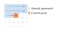
Under this ordering, the joint distribution of an image $𝒙$ is (Pixelrnn Factorisation) $\begin{matrix} p (𝒙) = \prod_{i = 1}^{H} \prod_{j = 1}^{W} p (x_{i, j, R} | 𝒙_{< (i, j)}) \cdot p (x_{i, j, G} | 𝒙_{< (i, j)}, x_{i, j, R}) \cdot p (x_{i, j, B} | 𝒙_{< (i, j)}, x_{i, j, R}, x_{i, j, G}) . \end{matrix}$

Row LSTM.

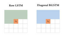
The Row LSTM processes each row of the image using a one-dimensional LSTM. The input to the LSTM at position $(i, j)$ is a feature vector computed from the pixel values above and to the left. The hidden state carries information along the row, while convolutional input-to-state connections provide context from the row above.

Receptive fields of the Row LSTM (left) and Diagonal BiLSTM (right). The Row LSTM's field is a cone that widens by one column per row climbed, so context outside it (red) is unreachable, and the missed region grows with distance from the current pixel; the Diagonal BiLSTM's two corner sweeps cover the entire context.

Diagonal BiLSTM.

The Diagonal BiLSTM extends the receptive field to cover all preceding pixels. It processes the image along diagonal directions, using two LSTMs that sweep from the top-left and top-right corners. This ensures that every preceding pixel can influence the prediction of the current pixel, at the cost of more complex computation.

Caution.

Generating an image with PixelRNN requires $D = H \times W \times C$ sequential LSTM steps. For a $256 \times 256$ RGB image, this means $256 \times 256 \times 3 = 196,608$ sequential steps, far too slow for practical applications. This motivated the development of PixelCNN, which replaces recurrence with (parallelisable) masked convolutions.

PixelCNN and Gated PixelCNN

PixelCNN [6][8] replaces the LSTM in PixelRNN with masked convolutional layers, enabling parallel computation during training while maintaining the autoregressive property.

Definition 9 (Masked convolution).

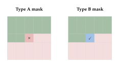
A masked convolution is a standard 2D convolution whose kernel is element-wise multiplied by a binary mask that zeroes out weights corresponding to “future” pixels (those that have not yet been generated in the raster-scan order). Two types are used:

Type A (first layer only): masks the centre pixel and all pixels below and to the right.
Type B (subsequent layers): masks pixels below and to the right, but includes the centre pixel (since hidden features at the current position do not violate causality).

Type A and Type B convolution masks for a

5 \times 5

kernel. Green cells have weight 1 (active); red cells have weight 0 (masked). Type A excludes the centre pixel; Type B includes it.

Proposition 4 (Blind spot).

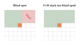
A stack of Type B masked convolutions has a blind spot: it cannot see pixels that are in the same column but in rows above the current pixel's row beyond the first row of the receptive field. Specifically, the effective receptive field forms an inverted triangle that misses the upper-right region of valid context.

This limitation is compositional rather than a property of any single mask: a Type B kernel does see the whole of the row above it. Reaching one column to the right, however, is only possible in the same step as moving one row up, so after a stack of layers the field can extend at most one column rightward for each row it climbs. Writing $a$ for the number of rows above the current pixel and $Δ c$ for the number of columns to its right, the reachable set is exactly ${Δ c \leq a}$ , at every depth. Stacking more layers grows the field upward but never relaxes that boundary, so the region ${Δ c > a}$ of valid context, an inverted triangle to the upper right, is excluded no matter how deep the network is.

Left: the blind spot problem in vanilla PixelCNN: the model cannot see the upper-right context region. Right: the vertical and horizontal stack architecture eliminates the blind spot.

Definition 10 (Vertical and horizontal stacks).

The Gated PixelCNN [8] solves the blind spot problem by splitting computation into two streams:

The vertical stack uses $k \times k$ convolutions that condition on the $k$ rows above the current row (no masking within those rows).
The horizontal stack uses $1 \times k$ row convolutions that condition on the current row up to (and including) the current pixel.

The vertical stack feeds into the horizontal stack at each layer, ensuring the horizontal stack has access to the full context above.

Gated activation

Definition 11 (Gated activation unit).

The Gated PixelCNN replaces the ReLU activation with a gated activation inspired by LSTMs: (Gated) $\begin{matrix} 𝒚 = \tanh (𝐖_{f} * 𝒙) ⊙ σ (𝐖_{g} * 𝒙), \end{matrix}$ where $*$ denotes convolution, $𝐖_{f}$ and $𝐖_{g}$ are learned filter banks, $\tanh$ provides the “content” and $σ$ provides the “gate” that controls information flow.

Modelling discrete pixel values

Since pixel values are integers in ${0, 1, \dots, 255}$ , the output of PixelCNN is typically a softmax over 256 values for each channel. However, this ignores the ordinal structure of pixel values.

Definition 12 (Discretised logistic mixture likelihood).

Salimans et al. [9] proposed modelling each (sub)pixel value with a mixture of logistic distributions, discretised to the pixel grid. For a mixture of $K$ logistics: (DISC Logistic) $\begin{matrix} p (x | 𝝅, 𝝁, 𝒔) = \sum_{k = 1}^{K} π_{k} [σ (\frac{x + 0.5 - μ_{k}}{s_{k}}) - σ (\frac{x - 0.5 - μ_{k}}{s_{k}})], \end{matrix}$ where the edge cases $x = 0$ and $x = 255$ are handled by extending the range to $- \infty$ and $+ \infty$ respectively.

Insight.

The discretised logistic mixture is a clever compromise: it respects the ordinal nature of pixel values (nearby values have similar probabilities) while remaining flexible through the mixture. Using just $K = 5$ mixture components typically suffices, reducing the output from 256 softmax logits to $3 K = 15$ parameters per subpixel.

WaveNet and Dilated Causal Convolutions

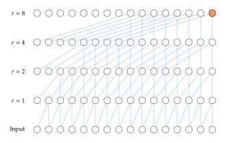
WaveNet [7] applied autoregressive modelling to raw audio waveforms, generating speech one sample at a time at 16 kHz. The key architectural innovation is the dilated causal convolution, which allows the receptive field to grow exponentially with depth.

Definition 13 (Dilated causal convolution).

A dilated causal convolution with dilation factor $r$ and kernel size $k$ computes (Dilated) $\begin{matrix} y_{t} = \sum_{i = 0}^{k - 1} w_{i} \cdot x_{t - r \cdot i}, \end{matrix}$ where the input is accessed at intervals of $r$ rather than at consecutive positions. The “causal” constraint means $y_{t}$ depends only on $x_{t^{'}}, t^{'} \leq t$ .

Dilated causal convolutions with dilation factors

r = 1, 2, 4, 8

and kernel size

k = 2

. The receptive field grows exponentially with depth: four layers cover 16 time steps.

Proposition 5 (Receptive field size).

A stack of $L$ dilated causal convolutions with kernel size $k$ and exponentially increasing dilation factors $r_{ℓ} = 2^{ℓ - 1}$ has a receptive field of size (Receptive Field) $\begin{matrix} R = (k - 1) \sum_{ℓ = 1}^{L} 2^{ℓ - 1} + 1 = (k - 1) (2^{L} - 1) + 1. \end{matrix}$

Proof.

Each layer $ℓ$ with dilation $r_{ℓ} = 2^{ℓ - 1}$ and kernel size $k$ extends the receptive field by $(k - 1) \cdot r_{ℓ}$ positions. The total extension over $L$ layers is $\sum_{ℓ = 1}^{L} (k - 1) \cdot 2^{ℓ - 1} = (k - 1) \sum_{ℓ = 0}^{L - 1} 2^{ℓ} = (k - 1) (2^{L} - 1) .$ Adding the initial position gives $R = (k - 1) (2^{L} - 1) + 1$ . For $k = 2$ and $L = 10$ , this yields $R = 1024$ , which covers about 64 ms of audio at 16 kHz.

∎

Example 2 (WaveNet for speech synthesis).

The original WaveNet [7] used 30 layers of dilated causal convolutions (three blocks of 10 layers with dilations $1, 2, 4, \dots, 512$ ), gated activations, residual connections, and skip connections. Audio samples were quantised to 256 levels using $μ$ -law companding and modelled with a 256-way softmax at each time step. The resulting speech was rated as significantly more natural than competing concatenative and parametric synthesis systems, approaching the quality of natural speech for the first time.

Training Autoregressive Models

Definition 14 (Teacher forcing).

Teacher forcing is the standard training strategy for autoregressive models: at each step $d$ , the model receives the ground-truth context $𝒙_{< d}$ as input, rather than its own predictions. The training objective is the negative log-likelihood: (Teacher Forcing) $\begin{matrix} ℒ (θ) = - \frac{1}{N} \sum_{n = 1}^{N} \sum_{d = 1}^{D} \log p_{θ} (x_{d}^{(n)} | 𝒙_{< d}^{(n)}) . \end{matrix}$

Teacher forcing enables fully parallel computation of all $D$ terms during training (using masked operations), but introduces a discrepancy between training and generation.

Definition 15 (Exposure bias).

Exposure bias is the mismatch between training (where the model sees ground-truth inputs) and generation (where it conditions on its own, potentially erroneous, predictions). Errors at early steps can cascade through the autoregressive chain, leading to poor sample quality.

Remark 2.

Exposure bias is most severe for long sequences and discrete outputs (e.g., text), where a single wrong token can derail the entire continuation. For images modelled with continuous outputs (e.g., discretised logistics), the effect is typically less pronounced because small errors do not propagate as catastrophically.

Scheduled sampling.

Bengio et al. [14] proposed scheduled sampling to bridge the gap: during training, with probability $ϵ_{t}$ (a curriculum schedule that increases from 0 to 1), the model conditions on its own prediction rather than the ground truth: (Scheduled Sampling) $\begin{matrix} {\tilde{x}}_{d - 1} = {\begin{matrix} x_{d - 1}^{(n)} & with probability 1 - ϵ_{t}, \\ {\hat{x}}_{d - 1} \sim p_{θ} (\cdot | 𝒙_{< d - 1}) & with probability ϵ_{t} . \end{matrix} \end{matrix}$

Caution.

Scheduled sampling does not optimise a consistent training objective; the targets are computed assuming ground-truth inputs, but the model sometimes sees its own outputs. Despite this inconsistency, it often improves generation quality in practice [10].

Modern Developments and Connections

The autoregressive principle has continued to drive advances in generative modelling. We briefly survey several important developments.

PixelSNAIL.

Chen et al. [15] combined masked convolutions with self-attention to create PixelSNAIL, which has access to all previously generated pixels through attention and local context through convolutions. PixelSNAIL achieved state-of-the-art density estimation on CIFAR-10 and ImageNet at the time of publication, demonstrating the power of combining local and global context.

ImageGPT.

Chen et al. [16] applied the GPT-2 Transformer architecture directly to sequences of pixel values (after clustering to a palette of 512 colours). ImageGPT demonstrated that the same autoregressive approach that works for language also works for images, achieving competitive generation quality and learning useful visual representations in an unsupervised manner.

Visual Autoregressive Modelling (VAR).

Tian et al. [17] proposed a paradigm shift: instead of generating images token by token, VAR generates images scale by scale, from coarse to fine resolution. The model first generates a low-resolution image, then progressively refines it at higher resolutions, with each scale conditioned on all previous scales. This “next-scale prediction” approach achieves state-of-the-art image generation quality while being significantly faster than traditional next-token autoregressive models, as it generates all tokens at each scale in parallel.

Key Idea.

The evolution from $n$ -grams to VAR illustrates a recurring theme: the autoregressive principle is universal and exact, but the ordering and architecture matter enormously. Traditional left-to-right or raster-scan orderings are natural but not necessarily optimal. Modern approaches explore hierarchical orderings (coarse-to-fine), attend to all context via Transformers, or combine autoregressive modelling with other paradigms (e.g., discrete tokenisation via VQ-VAE).

Timeline of autoregressive generative models, from Shannon's information theory (1948) to Visual Autoregressive Modelling (2024).

Connection to normalising flows.

Autoregressive models are closely connected to normalising flows (18). As we will see, the Masked Autoregressive Flow (MAF) uses the same autoregressive structure as MADE but interprets it as an invertible transformation, enabling both density evaluation and sampling through the change-of-variables formula.

Exercises

Exercise 1 (Chain rule and orderings).

Let $𝒙 = (x_{1}, x_{2}, x_{3})$ with joint distribution $p (x_{1}, x_{2}, x_{3})$ . Write down the autoregressive factorisation for the orderings $(1,2,3)$ , $(3,1,2)$ , and $(2,3,1)$ . Verify that each factorisation gives the same joint probability for any specific value of $𝒙$ .

Exercise 2 (Bigram perplexity).

A bigram model trained on a corpus gives the following probabilities for the sentence “the dog runs”: $p (the) = 0.1$ , $p (dog | the) = 0.02$ , $p (runs | dog) = 0.05$ . Compute the perplexity of this sentence under the model.

Exercise 3 (Laplace smoothing).

Consider a bigram model with vocabulary size $V = 10,000$ trained on a corpus where $count (the, cat) = 50$ and $count (the) = 5,000$ . Compute the smoothed probability $p_{α} (cat | the)$ for $α = 1$ (Laplace) and $α = 0.01$ . Compare both with the MLE estimate.

Exercise 4 (FVSBN parameter count).

Derive the total number of parameters in an FVSBN for binary data of dimension $D$ . Compare this with the number of parameters in a NADE with $H$ hidden units. For what value of $H$ does NADE have fewer parameters than FVSBN?

Exercise 5 (NADE log-likelihood).

Implement the NADE forward pass (Algorithm 1) in pseudocode for continuous data using a Gaussian output distribution $p (x_{d} | 𝒙_{< d}) = 𝒩 (x_{d}; μ_{d}, σ_{d}^{2})$ , where $μ_{d}$ and $\log σ_{d}$ are linear functions of $𝒉_{d}$ . Write out the log-likelihood expression.

Exercise 6 (MADE mask construction).

For $D = 4$ inputs, one hidden layer with 6 units, and the ordering $(1,2,3,4)$ :

Assign connectivity numbers to hidden units (using the rule $m (k) \sim Uniform {1, \dots, D - 1}$ ) and construct the input-to-hidden and hidden-to-output masks.
Verify that output 3 depends only on inputs 1 and 2.
How many connectivity-number assignments are valid?

Exercise 7 (Masked convolution receptive field).

Show that a stack of $L$ Type B masked convolutions with $k \times k$ kernels has a receptive field of height $⌊ k / 2 ⌋ \cdot L + 1$ rows above the current pixel. What is the receptive field width?

Exercise 8 (Blind spot verification).

For a $3 \times 3$ kernel, draw the effective receptive field after $L = 1, 2, 3$ layers of Type B masked convolutions. Identify the blind spot region and verify that it grows with $L$ .

Exercise 9 (WaveNet receptive field).

A WaveNet model uses three blocks, each containing 10 layers of dilated causal convolutions with kernel size $k = 2$ and dilations $r = 1, 2, 4, \dots, 512$ . Calculate the total receptive field in time steps and in milliseconds at 16 kHz.

Exercise 10 (Gated activation vs ReLU).

Consider the gated activation $y = \tanh (W_{f} x) ⊙ σ (W_{g} x)$ and the ReLU activation $y = \max (0, W x)$ .

Show that the gated activation can represent any function the ReLU can represent (in a single-layer, single-unit setting).
Give an example of a function the gated unit can represent but a single ReLU unit cannot.

Exercise 11 (Discretised logistic likelihood).

For a single logistic distribution with mean $μ = 128$ and scale $s = 10$ , compute $p (x = 128)$ and $p (x = 0)$ using the discretised logistic formula in (DISC Logistic).

Exercise 12 (Exposure bias simulation).

Consider a simple autoregressive model over ${0,1}^{D}$ where each conditional has accuracy $1 - ϵ$ (i.e., it predicts the correct value with probability $1 - ϵ$ ). Assuming errors are independent, derive the probability that the entire generated sequence is correct. For $D = 1000$ and $ϵ = 0.01$ , what is this probability?

Exercise 13 (Interpolation weights).

Describe how you would use a held-out validation set to optimise the interpolation weights $λ_{1}, λ_{2}, λ_{3}$ in (Interpolation). What constraint must the weights satisfy? Suggest an optimisation algorithm.

Exercise 14 (Autoregressive models and Bayesian networks).

Show that any autoregressive model defines a Bayesian network with a specific DAG structure. What is the in-degree of node $d$ in this DAG? Under what conditions does the autoregressive model reduce to a fully factored (independent) model?

Exercise 15 (Cross-entropy and KL divergence).

Prove that for two distributions $p$ and $q$ over a finite alphabet, $𝖧 (p, q) = 𝖧 (p) + 𝖣_{KL} (p ‖ q)$ . Use this to explain why minimising the cross-entropy loss in autoregressive models is equivalent to minimising the KL divergence from the data distribution to the model.

References

A mathematical theory of communication

Claude Elwood Shannon

The Bell System Technical Journal, vol. 27, no. 3, pp. 379-423 · 1948

BibTeX

@article{shannon1948mathematical,
  title={A mathematical theory of communication},
  author={Shannon, Claude Elwood},
  journal={The Bell System Technical Journal},
  volume={27},
  number={3},
  pages={379--423},
  year={1948},
  publisher={Nokia Bell Labs}
}

Journal article

Prediction and Entropy of Printed English

Claude E. Shannon

Bell System Technical Journal, vol. 30, no. 1, pp. 50-64 · 1951

BibTeX

@article{shannon1951prediction,
  title={Prediction and Entropy of Printed {English}},
  author={Shannon, Claude E.},
  journal={Bell System Technical Journal},
  volume={30},
  number={1},
  pages={50--64},
  year={1951}
}

Journal article

A Neural Probabilistic Language Model

Yoshua Bengio, Rejean Ducharme, Pascal Vincent, Christian Jauvin

Journal of Machine Learning Research, vol. 3, pp. 1137-1155 · 2003

BibTeX

@article{bengio2003neural,
  title={A Neural Probabilistic Language Model},
  author={Bengio, Yoshua and Ducharme, R\'{e}jean and Vincent, Pascal and Jauvin, Christian},
  journal={Journal of Machine Learning Research},
  volume={3},
  pages={1137--1155},
  year={2003}
}

Journal article

The Neural Autoregressive Distribution Estimator

Hugo Larochelle, Iain Murray

Proceedings of the 14th International Conference on Artificial Intelligence and Statistics (AISTATS) · 2011

BibTeX

@inproceedings{larochelle2011neural,
  title={The Neural Autoregressive Distribution Estimator},
  author={Larochelle, Hugo and Murray, Iain},
  booktitle={Proceedings of the 14th International Conference on Artificial Intelligence and Statistics (AISTATS)},
  year={2011}
}

Conference paper

MADE: Masked Autoencoder for Distribution Estimation

Mathieu Germain, Karol Gregor, Iain Murray, Hugo Larochelle

Proceedings of the 32nd International Conference on Machine Learning (ICML) · 2015

BibTeX

@inproceedings{germain2015made,
  title={{MADE}: Masked Autoencoder for Distribution Estimation},
  author={Germain, Mathieu and Gregor, Karol and Murray, Iain and Larochelle, Hugo},
  booktitle={Proceedings of the 32nd International Conference on Machine Learning (ICML)},
  year={2015}
}

Conference paper

Pixel Recurrent Neural Networks

Aaron van den Oord, Nal Kalchbrenner, Koray Kavukcuoglu

Proceedings of the 33rd International Conference on Machine Learning (ICML) · 2016

BibTeX

@inproceedings{oord2016pixel,
  title={Pixel Recurrent Neural Networks},
  author={van den Oord, A\"{a}ron and Kalchbrenner, Nal and Kavukcuoglu, Koray},
  booktitle={Proceedings of the 33rd International Conference on Machine Learning (ICML)},
  year={2016}
}

Conference paper

WaveNet: A Generative Model for Raw Audio

Aaron van den Oord, Sander Dieleman, Heiga Zen, Karen Simonyan, Oriol Vinyals, Alex Graves, Nal Kalchbrenner, Andrew Senior, et al.

arXiv preprint arXiv:1609.03499 · 2016

BibTeX

@article{oord2016wavenet,
  author    = {van den Oord, Aaron and Dieleman, Sander and Zen, Heiga and Simonyan, Karen and Vinyals, Oriol and Graves, Alex and Kalchbrenner, Nal and Senior, Andrew and Kavukcuoglu, Koray},
  title     = {{WaveNet}: A Generative Model for Raw Audio},
  journal   = {arXiv preprint arXiv:1609.03499},
  year      = {2016}
}

Journal article

Conditional Image Generation with PixelCNN Decoders

Aaron van den Oord, Nal Kalchbrenner, Lasse Espeholt, Koray Kavukcuoglu, Oriol Vinyals, Alex Graves

Advances in Neural Information Processing Systems (NeurIPS) · 2016

BibTeX

@inproceedings{oord2016conditional,
  title={Conditional Image Generation with {PixelCNN} Decoders},
  author={van den Oord, A\"{a}ron and Kalchbrenner, Nal and Espeholt, Lasse and Kavukcuoglu, Koray and Vinyals, Oriol and Graves, Alex},
  booktitle={Advances in Neural Information Processing Systems (NeurIPS)},
  year={2016}
}

Conference paper

PixelCNN++: Improving the PixelCNN with Discretized Logistic Mixture Likelihood and Other Modifications

Tim Salimans, Andrej Karpathy, Xi Chen, Diederik P. Kingma

International Conference on Learning Representations (ICLR) · 2017

BibTeX

@inproceedings{salimans2017pixelcnn,
  title={{PixelCNN++}: Improving the {PixelCNN} with Discretized Logistic Mixture Likelihood and Other Modifications},
  author={Salimans, Tim and Karpathy, Andrej and Chen, Xi and Kingma, Diederik P.},
  booktitle={International Conference on Learning Representations (ICLR)},
  year={2017}
}

Conference paper

Professor Forcing: A New Algorithm for Training Recurrent Networks

Alex M. Lamb, Anirudh Goyal, Ying Zhang, Saizheng Zhang, Aaron Courville, Yoshua Bengio

Advances in Neural Information Processing Systems (NeurIPS) · 2016

BibTeX

@inproceedings{lamb2016professor,
  title={Professor Forcing: A New Algorithm for Training Recurrent Networks},
  author={Lamb, Alex M. and Goyal, Anirudh and Zhang, Ying and Zhang, Saizheng and Courville, Aaron and Bengio, Yoshua},
  booktitle={Advances in Neural Information Processing Systems (NeurIPS)},
  year={2016}
}

Conference paper

Connectionist Learning of Belief Networks

Radford M. Neal

Artificial Intelligence, vol. 56, no. 1, pp. 71-113 · 1992

BibTeX

@article{neal1992connectionist,
  title={Connectionist Learning of Belief Networks},
  author={Neal, Radford M.},
  journal={Artificial Intelligence},
  volume={56},
  number={1},
  pages={71--113},
  year={1992}
}

Journal article

A Deep and Tractable Density Estimator

Benigno Uria, Iain Murray, Hugo Larochelle

Proceedings of the 31st International Conference on Machine Learning (ICML) · 2014

BibTeX

@inproceedings{uria2014deep,
  title={A Deep and Tractable Density Estimator},
  author={Uria, Benigno and Murray, Iain and Larochelle, Hugo},
  booktitle={Proceedings of the 31st International Conference on Machine Learning (ICML)},
  year={2014}
}

Conference paper

Neural Autoregressive Distribution Estimation

Benigno Uria, Marc-Alexandre Cote, Karol Gregor, Iain Murray, Hugo Larochelle

Journal of Machine Learning Research, vol. 17, no. 205, pp. 1-37 · 2016

BibTeX

@article{uria2016neural,
  title={Neural Autoregressive Distribution Estimation},
  author={Uria, Benigno and C\^{o}t\'{e}, Marc-Alexandre and Gregor, Karol and Murray, Iain and Larochelle, Hugo},
  journal={Journal of Machine Learning Research},
  volume={17},
  number={205},
  pages={1--37},
  year={2016}
}

Journal article

Scheduled Sampling for Sequence Prediction with Recurrent Neural Networks

Samy Bengio, Oriol Vinyals, Navdeep Jaitly, Noam Shazeer

Advances in Neural Information Processing Systems (NeurIPS) · 2015

BibTeX

@inproceedings{bengio2015scheduled,
  title={Scheduled Sampling for Sequence Prediction with Recurrent Neural Networks},
  author={Bengio, Samy and Vinyals, Oriol and Jaitly, Navdeep and Shazeer, Noam},
  booktitle={Advances in Neural Information Processing Systems (NeurIPS)},
  year={2015}
}

Conference paper

PixelSNAIL: An Improved Autoregressive Generative Model

Xi Chen, Nikhil Mishra, Mostafa Rohaninejad, Pieter Abbeel

Proceedings of the 35th International Conference on Machine Learning (ICML) · 2018

BibTeX

@inproceedings{chen2018pixelsnail,
  title={{PixelSNAIL}: An Improved Autoregressive Generative Model},
  author={Chen, Xi and Mishra, Nikhil and Rohaninejad, Mostafa and Abbeel, Pieter},
  booktitle={Proceedings of the 35th International Conference on Machine Learning (ICML)},
  year={2018}
}

Conference paper

Generative Pretraining from Pixels

Mark Chen, Alec Radford, Rewon Child, Jeff Wu, Heewoo Jun, David Luan, Ilya Sutskever

Proceedings of the 37th International Conference on Machine Learning (ICML) · 2020

BibTeX

@inproceedings{chen2020generative,
  title={Generative Pretraining from Pixels},
  author={Chen, Mark and Radford, Alec and Child, Rewon and Wu, Jeff and Jun, Heewoo and Luan, David and Sutskever, Ilya},
  booktitle={Proceedings of the 37th International Conference on Machine Learning (ICML)},
  year={2020}
}

Conference paper

Visual Autoregressive Modeling: Scalable Image Generation via Next-Scale Prediction

Keyu Tian, Yi Jiang, Zehuan Yuan, Bingyue Peng, Liwei Wang

Advances in Neural Information Processing Systems (NeurIPS) · 2024

BibTeX

@inproceedings{tian2024visual,
  title={Visual Autoregressive Modeling: Scalable Image Generation via Next-Scale Prediction},
  author={Tian, Keyu and Jiang, Yi and Yuan, Zehuan and Peng, Bingyue and Wang, Liwei},
  booktitle={Advances in Neural Information Processing Systems (NeurIPS)},
  year={2024}
}

Conference paper

← 16 Advanced VAE Variants 18 Normalizing Flows →

17 Autoregressive Models

The Chain Rule and Autoregressive Factorisation

Training by maximum likelihood.

Generation.

N-gram Language Models

The sparsity problem

Smoothing techniques

Perplexity

Fully-Visible Sigmoid Belief Networks

NADE: Neural Autoregressive Density Estimation

Deep NADE.

NADE for continuous data.

MADE: Masked Autoencoders for Distribution Estimation

Constructing the masks.

Order agnosticism.

PixelRNN

Row LSTM.

Diagonal BiLSTM.

PixelCNN and Gated PixelCNN

The blind spot problem

Gated activation

Modelling discrete pixel values

WaveNet and Dilated Causal Convolutions

Training Autoregressive Models

Scheduled sampling.

Modern Developments and Connections

PixelSNAIL.

ImageGPT.

Visual Autoregressive Modelling (VAR).

Connection to normalising flows.

Exercises

References

$N$ -gram Language Models