18 Normalizing Flows

In the previous chapter we saw that autoregressive models provide exact likelihoods by factorising a joint distribution into one-dimensional conditionals. Normalizing flows take a different route: they transform a simple base distribution (typically a standard Gaussian) through a sequence of invertible mappings, and use the change-of-variables formula to compute the density of the transformed distribution exactly.

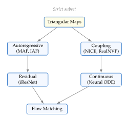
The central trade-off is architectural: every transformation must be invertible and its Jacobian determinant must be efficiently computable. This constraint has inspired a rich family of architectures, from coupling layers to continuous-time flows, that we develop in this chapter:

We begin with the change-of-variables formula and the mathematical foundations of normalizing flows.
We introduce coupling flows: NICE and RealNVP.
We study Glow and invertible $1 \times 1$ convolutions.
We develop autoregressive flows: MAF and IAF, and their duality.
We present neural spline flows for flexible monotonic transformations.
We discuss residual flows and their connection to the Banach fixed-point theorem.
We introduce continuous normalizing flows: neural ODEs and FFJORD.
We develop flow matching, a simulation-free training method that has become the foundation for modern generative models.
We survey connections and applications to other generative paradigms.

Historical Note.

The idea of transporting one probability distribution to another through smooth maps dates back to Monge (1781) and was formalised by Kantorovich in the 1940s in the context of optimal transport (14). Tabak and Vanden-Eijnden [1] proposed using normalizing flows for density estimation in 2010. Rezende and Mohamed [2] introduced normalizing flows into the deep learning framework in 2015 for variational inference. The subsequent years saw rapid development: NICE [3] (2014), RealNVP [4] (2016), Glow [5] (2018), Neural ODEs [6] and FFJORD [7] (2018–2019), and flow matching [8] (2022), which now underlies state-of-the-art image and video generation systems.

Change of Variables and Flow Foundations

The change-of-variables formula

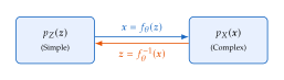
Let $𝒛 \in ℝ^{D}$ be a random vector with density $p_{Z} (𝒛)$ , and let $f : ℝ^{D} \to ℝ^{D}$ be a diffeomorphism, a smooth, invertible map whose inverse is also smooth. The transformed variable $𝒙 = f (𝒛)$ has density given by the change-of-variables formula.

Definition 1 (Normalizing flow).

A normalizing flow is a diffeomorphism $f_{θ} : ℝ^{D} \to ℝ^{D}$ (parameterised by $θ$ ) that transforms a base density $p_{Z}$ into a model density $p_{X}$ . The density of $𝒙 = f_{θ} (𝒛)$ is (COV) $\begin{matrix} p_{X} (𝒙) = p_{Z} (f_{θ}^{- 1} (𝒙)) | \det \frac{\partial f_{θ}^{- 1} (𝒙)}{\partial 𝒙} | = p_{Z} (𝒛) | \det \frac{\partial f_{θ} (𝒛)}{\partial 𝒛} |^{- 1}, \end{matrix}$ where $\frac{\partial f_{θ}}{\partial 𝒛} \in ℝ^{D \times D}$ is the Jacobian matrix.

Taking logarithms, the log-likelihood of a data point $𝒙$ is (LOG Likelihood) $\begin{matrix} \log p_{X} (𝒙) = \log p_{Z} (f_{θ}^{- 1} (𝒙)) + \log | \det \frac{\partial f_{θ}^{- 1}}{\partial 𝒙} (𝒙) | . \end{matrix}$ The two computational requirements are clear:

We need to invert $f_{θ}$ to compute $𝒛 = f_{θ}^{- 1} (𝒙)$ .
We need the log-determinant of the Jacobian.

A normalizing flow transforms a simple base density

p_{Z}

(e.g., standard Gaussian) into a complex data density

p_{X}

through an invertible map

f_{θ}

. The forward map generates samples; the inverse map computes likelihoods.

Composing flows

In practice, a single transformation is too simple to model complex data. We compose $K$ transformations:

Theorem 1 (Composition of flows).

Let $f = f_{K} \circ f_{K - 1} \circ \dots \circ f_{1}$ be a composition of diffeomorphisms $f_{k} : ℝ^{D} \to ℝ^{D}$ . Then $f$ is a diffeomorphism and (Composition) $\begin{matrix} \log p_{X} (𝒙) = \log p_{Z} (𝒛_{0}) - \sum_{k = 1}^{K} \log | \det \frac{\partial f_{k}}{\partial 𝒛_{k - 1}} (𝒛_{k - 1}) |, \end{matrix}$ where $𝒛_{0} = f^{- 1} (𝒙)$ and $𝒛_{k} = f_{k} (𝒛_{k - 1})$ .

Proof.

By the chain rule for Jacobians, $\frac{\partial f}{\partial 𝒛_{0}} = \frac{\partial f_{K}}{\partial 𝒛_{K - 1}} \dots \frac{\partial f_{1}}{\partial 𝒛_{0}}$ . Taking determinants and using $\det (A B) = \det (A) \det (B)$ gives $\det \frac{\partial f}{\partial 𝒛_{0}} = \prod_{k = 1}^{K} \det \frac{\partial f_{k}}{\partial 𝒛_{k - 1}}$ . Taking logarithms and absolute values yields the result.

∎

Triangular maps and the Knothe–Rosenblatt rearrangement

Computing the determinant of a general $D \times D$ matrix costs $𝒪 (D^{3})$ , which is prohibitive for high-dimensional data. The key to efficient flows is to design transformations whose Jacobians are triangular.

Definition 2 (Triangular map).

A map $f : ℝ^{D} \to ℝ^{D}$ is lower triangular if $f_{d} (𝒛)$ depends only on $z_{1}, \dots, z_{d}$ : $f_{d} (𝒛) = f_{d} (z_{1}, \dots, z_{d}) .$ The Jacobian is then lower triangular, and its determinant is simply the product of diagonal entries: (Triangular DET) $\begin{matrix} \det \frac{\partial f}{\partial 𝒛} = \prod_{d = 1}^{D} \frac{\partial f_{d}}{\partial z_{d}}, \end{matrix}$ which costs only $𝒪 (D)$ .

Theorem 2 (Knothe–Rosenblatt rearrangement).

Let $p$ and $q$ be two absolutely continuous probability distributions on $ℝ^{D}$ with positive densities. There exists a unique lower triangular map $T : ℝ^{D} \to ℝ^{D}$ with $T_{d}$ increasing in $z_{d}$ (for each fixed $z_{1}, \dots, z_{d - 1}$ ) such that $T_{#} p = q$ (i.e., $T$ pushes $p$ forward to $q$ ).

Proof sketch.

The proof proceeds by induction on $D$ . For $D = 1$ , the map is the composition of the CDF of $p$ with the quantile function of $q$ : $T_{1} = F_{q}^{- 1} \circ F_{p}$ . For general $D$ , we first map the marginal of $z_{1}$ under $p$ to the marginal under $q$ using the one-dimensional result, then conditioned on the transformed first coordinate, map the conditional of $z_{2}$ under $p$ to the conditional under $q$ , and so on. Uniqueness follows from the monotonicity constraint.

∎

Corollary 1 (Universal approximation).

Triangular flows are universal: for any two sufficiently regular distributions $p$ and $q$ , there exists a triangular map that transforms $p$ into $q$ . In particular, any distribution can be represented as a triangular transformation of a standard Gaussian.

Key Idea.

The Knothe–Rosenblatt theorem is the theoretical foundation of normalizing flows: it guarantees that triangular maps are universal: they can represent any continuous distribution as a transformation of a simple base distribution. All practical flow architectures (coupling layers, autoregressive flows) are special cases of triangular maps.

Taxonomy of normalizing flow architectures. Coupling and autoregressive flows are special cases of triangular maps. Residual and continuous flows relax the triangular structure. Flow matching unifies several approaches.

Coupling Flows: NICE and RealNVP

The simplest way to build an invertible transformation with a cheap Jacobian determinant is to split the input into two groups and transform one group as a function of the other.

Definition 3 (Affine coupling layer).

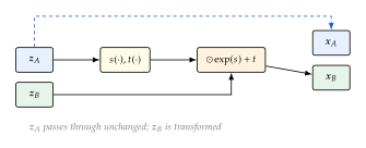
An affine coupling layer splits the input $𝒛 \in ℝ^{D}$ into two disjoint parts $𝒛 = (𝒛_{A}, 𝒛_{B})$ (with $| 𝒛_{A} | = d$ and $| 𝒛_{B} | = D - d$ ) and applies (Coupling) $\begin{matrix} 𝒙_{A} = 𝒛_{A}, 𝒙_{B} = 𝒛_{B} ⊙ \exp (s (𝒛_{A})) + t (𝒛_{A}), \end{matrix}$ where $s, t : ℝ^{d} \to ℝ^{D - d}$ are arbitrary neural networks (the “scale” and “translation” networks).

Proposition 1 (Coupling layer Jacobian).

The Jacobian of the affine coupling layer is lower triangular (after appropriate ordering) with determinant (Coupling DET) $\begin{matrix} \det \frac{\partial 𝒙}{\partial 𝒛} = \prod_{j = 1}^{D - d} \exp (s_{j} (𝒛_{A})) = \exp (\sum_{j = 1}^{D - d} s_{j} (𝒛_{A})) . \end{matrix}$ The log-determinant is therefore simply $\sum_{j = 1}^{D - d} s_{j} (𝒛_{A})$ , a sum of the scale network outputs.

Proof.

The Jacobian has the block structure $\frac{\partial 𝒙}{\partial 𝒛} = (\begin{matrix} 𝐈_{d} & 𝟎 \\ \frac{\partial 𝒙_{B}}{\partial 𝒛_{A}} & diag (\exp (s (𝒛_{A}))) \end{matrix}) .$ This is lower block-triangular, so its determinant is the product of the determinants of the diagonal blocks: $\det (𝐈_{d}) \cdot \det (diag (\exp (s (𝒛_{A})))) = \prod_{j} \exp (s_{j} (𝒛_{A}))$ .

∎

The inverse is equally simple: $𝒛_{A} = 𝒙_{A}$ and $𝒛_{B} = (𝒙_{B} - t (𝒙_{A})) ⊙ \exp (- s (𝒙_{A}))$ .

Affine coupling layer. The “pass-through” partition

𝒛_{A}

is unchanged and used to parameterise the transformation of

𝒛_{B}

. The networks

s (\cdot)

and

t (\cdot)

can be arbitrarily complex without affecting invertibility.

NICE

Definition 4 (NICE).

NICE (Non-linear Independent Components Estimation) [3] is a coupling flow where the scale function is set to zero ( $s \equiv 0$ ), giving a volume-preserving additive coupling: $\begin{matrix} 𝒙_{A} = 𝒛_{A}, 𝒙_{B} = 𝒛_{B} + t (𝒛_{A}) . \end{matrix}$ The Jacobian determinant is identically 1, so the log-likelihood simplifies to $\log p_{X} (𝒙) = \log p_{Z} (f^{- 1} (𝒙))$ .

Remark 1.

Because each NICE layer is volume-preserving, the model cannot change the volume of regions in space. To compensate, NICE uses a learnable diagonal scaling matrix at the end of the flow. RealNVP removes this limitation by introducing the scale function $s$ .

RealNVP and multi-scale architecture

Definition 5 (Multi-scale architecture).

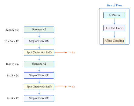
RealNVP [4] introduces a multi-scale architecture where, after a block of coupling layers at each resolution, half of the dimensions are “factored out” (directly modelled by the base distribution) and the remaining dimensions continue to the next block at the same resolution. This progressively reduces the computational cost and allows the model to capture features at different scales.

Masking patterns for image coupling layers. Left: checkerboard spatial masking alternates which pixels belong to

𝒛_{A}

and

𝒛_{B}

. Right: channel-wise masking splits along the channel dimension after a squeeze operation.

Example 1 (RealNVP on 2D data).

Consider $𝒛 = (z_{1}, z_{2}) \sim 𝒩 (0, 𝐈_{2})$ . By alternating which dimension is transformed, a stack of coupling layers can learn to map the isotropic Gaussian to complex 2D distributions such as two moons or concentric rings. Despite using simple affine transformations, the alternating structure allows each dimension to be transformed as a function of the other, building up expressive power through composition.

Two layers alone are not enough for targets of this kind. After a layer that moves $z_{2}$ while reading $z_{1}$ , the mass concentrates near a graph over the $z_{1}$ axis, and a single following layer that moves $z_{1}$ can only rescale and shift it by functions of the other coordinate, so the result remains a graph over one axis. Two moons and concentric rings are graphs over neither axis, so at least two full alternations (four coupling layers) are required, and practical models use many more.

Caution.

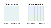
A single coupling layer can only transform the $B$ -partition as a function of the $A$ -partition. If we always split the same way, the $A$ -partition is never transformed. In practice, we must alternate which dimensions are passed through and which are transformed. RealNVP alternates between checkerboard and channel-wise masking patterns at each layer.

Glow and Invertible $1 \times 1$ Convolutions

Kingma and Dhariwal [5] proposed Glow, an improved flow architecture that replaces fixed permutations with learnable invertible $1 \times 1$ convolutions and adds activation normalisation for stable training.

Definition 6 (Invertible $1 \times 1$ convolution).

An invertible $1 \times 1$ convolution is a linear transformation $𝒙 = 𝐖 𝒛$ applied independently at each spatial position, where $𝐖 \in ℝ^{C \times C}$ is an invertible matrix ( $C$ is the number of channels). The log-determinant contribution at each spatial position is $\log | \det 𝐖 |$ , and for an $H \times W$ feature map the total is (1X1 DET) $\begin{matrix} \log | \det \frac{\partial 𝒙}{\partial 𝒛} | = H \cdot W \cdot \log | \det 𝐖 | . \end{matrix}$

Proposition 2 (LU decomposition for efficient computation).

Computing $\det 𝐖$ naively costs $𝒪 (C^{3})$ . By parameterising $𝐖 = 𝐏 𝐋 𝐔$ where $𝐏$ is a fixed permutation matrix, $𝐋$ is lower triangular with ones on the diagonal, and $𝐔$ is upper triangular, the determinant reduces to $\begin{matrix} \log | \det 𝐖 | = \sum_{c = 1}^{C} \log | U_{c c} |, \end{matrix}$ which costs only $𝒪 (C)$ .

Proof.

Since $\det 𝐏 = \pm 1$ and $\det 𝐋 = 1$ (ones on diagonal), we have $\det 𝐖 = \det 𝐏 \cdot \det 𝐋 \cdot \det 𝐔 = \pm \prod_{c = 1}^{C} U_{c c}$ . Taking absolute values and logarithms gives the result.

∎

Definition 7 (Activation normalisation (ActNorm)).

ActNorm is an invertible affine transformation $𝒙 = 𝒔 ⊙ 𝒛 + 𝒃$ (per channel), where the scale $𝒔$ and bias $𝒃$ are initialised so that the output has zero mean and unit variance on the first minibatch (data-dependent initialisation), then treated as learnable parameters. It serves as a replacement for batch normalisation that is exactly invertible.

Algorithm 1 (One step of Glow).

Each step of flow in Glow consists of three sub-layers applied in sequence:

Input: Feature map $𝒛 \in ℝ^{H \times W \times C}$
ActNorm: $𝒉_{1} = 𝒔 ⊙ 𝒛 + 𝒃$ Affine, per channel
Inv. $1 \times 1$ conv: $𝒉_{2} = 𝐖 𝒉_{1}$ Channel mixing
Affine coupling: $𝒙 = AffineCoupling (𝒉_{2})$ Split channels
return $𝒙$

Glow multi-scale architecture. The “squeeze” operation reshapes spatial dimensions into channels (

H / 2 \times W / 2 \times 4 C

). After each level, half the channels are factored out and modelled directly by the base distribution. Each “step of flow” consists of ActNorm, an invertible

1 \times 1

convolution, and an affine coupling layer.

Autoregressive Flows: MAF and IAF

Autoregressive flows connect the autoregressive models of 17 with normalizing flows. The key insight is that an autoregressive model defines a triangular map, and triangular maps are invertible with cheap determinants.

Definition 8 (Masked Autoregressive Flow (MAF)).

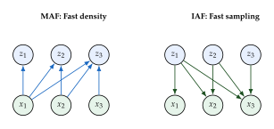
A Masked Autoregressive Flow [9] transforms $𝒛 \to 𝒙$ by (MAF) $\begin{matrix} x_{d} = z_{d} \cdot \exp (s_{d} (𝒙_{< d})) + t_{d} (𝒙_{< d}), d = 1, \dots, D, \end{matrix}$ where $s_{d}$ and $t_{d}$ are computed by a MADE-style masked network. The generation direction ( $𝒛 \to 𝒙$ ) is sequential: each $x_{d}$ depends on all previous $x_{< d}$ . The density evaluation direction ( $𝒙 \to 𝒛$ ) is parallel: given $𝒙$ , all $z_{d}$ can be computed simultaneously.

Definition 9 (Inverse Autoregressive Flow (IAF)).

An Inverse Autoregressive Flow [10] transforms $𝒛 \to 𝒙$ by (IAF) $\begin{matrix} x_{d} = z_{d} \cdot \exp (s_{d} (𝒛_{< d})) + t_{d} (𝒛_{< d}), d = 1, \dots, D, \end{matrix}$ where $s_{d}$ and $t_{d}$ depend on the input $𝒛_{< d}$ rather than the output. Generation ( $𝒛 \to 𝒙$ ) is now parallel, but density evaluation ( $𝒙 \to 𝒛$ ) requires sequential inversion.

Theorem 3 (MAF–IAF duality).

MAF and IAF are inverses of each other: the forward pass of MAF is the inverse pass of IAF, and vice versa. Specifically:

	Density eval. ( $𝒙 \to 𝒛$ )	Sampling ( $𝒛 \to 𝒙$ )
MAF	Parallel ( $𝒪 (1)$ depth)	Sequential ( $𝒪 (D)$ depth)
IAF	Sequential ( $𝒪 (D)$ depth)	Parallel ( $𝒪 (1)$ depth)

Proof.

Consider the MAF forward map $x_{d} = z_{d} \exp (s_{d} (𝒙_{< d})) + t_{d} (𝒙_{< d})$ . Given $𝒙$ , we can compute all $z_{d}$ in parallel via $z_{d} = (x_{d} - t_{d} (𝒙_{< d})) \exp (- s_{d} (𝒙_{< d}))$ . Relabelling the roles of $𝒙$ and $𝒛$ , this is an IAF forward map with conditioner outputs ${\tilde{s}}_{d} = - s_{d} (𝒛_{< d})$ and ${\tilde{t}}_{d} = - t_{d} (𝒛_{< d}) \exp (- s_{d} (𝒛_{< d}))$ ; since both are themselves arbitrary functions of the preceding coordinates, they are legitimate outputs of an IAF conditioner, so the two families coincide. The Jacobian in both cases is triangular with diagonal entries $\exp (s_{d} (\cdot))$ , confirming they share the same determinant structure.

∎

MAF vs IAF for

D = 3

. Left (MAF): density evaluation is parallel: all

z_{d}

can be computed from

𝒙

simultaneously. Right (IAF): sampling is parallel: all

x_{d}

can be computed from

𝒛

simultaneously. Each is the inverse of the other.

Proposition 3 (Autoregressive Jacobian).

For both MAF and IAF, the Jacobian is lower triangular with diagonal entries $\exp (s_{d} (\cdot))$ . The log-determinant is (Autoreg Logdet) $\begin{matrix} \log | \det \frac{\partial 𝒙}{\partial 𝒛} | = \sum_{d = 1}^{D} s_{d} (\cdot) . \end{matrix}$

Proof.

Since $x_{d}$ depends on $z_{d}$ only through the affine transformation $x_{d} = z_{d} \exp (s_{d}) + t_{d}$ , the partial derivative $\partial x_{d} / \partial z_{d} = \exp (s_{d})$ . For $d^{'} < d$ , the dependence of $x_{d}$ on $z_{d^{'}}$ is only through the conditioning variables $𝒙_{< d}$ (for MAF) or $𝒛_{< d}$ (for IAF), and these contribute only to the lower-triangular part. The determinant of a triangular matrix is the product of its diagonal entries.

∎

Insight.

MAF is ideal for training (density estimation), where fast likelihood computation is needed. IAF is ideal for inference in VAEs, where fast sampling from the approximate posterior is needed. This complementarity is the reason both variants exist and are used in different contexts.

Neural Spline Flows

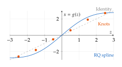
Affine coupling and autoregressive layers are limited in their element-wise expressiveness: each $z_{d} \mapsto x_{d}$ is an affine function (for fixed conditioning variables). Durkan et al. [14] proposed replacing affine transformations with monotone rational-quadratic splines, dramatically increasing per-layer expressiveness.

Definition 10 (Rational-quadratic spline transformer).

A rational-quadratic (RQ) spline is a piecewise function defined on $K$ bins $[b_{k - 1}, b_{k}]$ , where each piece is a rational-quadratic function (ratio of two quadratics). The spline is parameterised by:

Bin widths ${w_{k}}_{k = 1}^{K}$ (positive, summing to the interval width),
Bin heights ${h_{k}}_{k = 1}^{K}$ (positive, summing to the output interval width),
Derivatives at knots ${d_{k}}_{k = 0}^{K}$ (positive, ensuring monotonicity).

The bin widths and heights are produced by a softmax from the conditioning network, and the derivatives by a softplus.

Proposition 4 (Monotonicity of RQ splines).

A rational-quadratic spline with positive derivatives at all knots $d_{k} > 0$ is strictly monotonically increasing on each bin, hence invertible. The derivative (needed for the Jacobian) has a closed-form expression within each bin.

Proof.

Within bin $[b_{k - 1}, b_{k}]$ , the rational-quadratic function is $g (ξ) = h_{k - 1} + \frac{(h_{k} - h_{k - 1}) (s_{k} ξ^{2} + d_{k - 1} ξ (1 - ξ))}{s_{k} + (d_{k - 1} + d_{k} - 2 s_{k}) ξ (1 - ξ)},$ where $ξ = (z - b_{k - 1}) / (b_{k} - b_{k - 1}) \in [0,1]$ and $s_{k} = (h_{k} - h_{k - 1}) / (b_{k} - b_{k - 1})$ is the bin slope. Here $h_{k - 1}$ and $h_{k}$ denote the cumulative knot values (the output coordinates of the two knots bounding the bin), so that $g (0) = h_{k - 1}$ and $g (1) = h_{k}$ ; the bin height of Definition 10 is the difference $h_{k} - h_{k - 1}$ . Differentiating and converting from $ξ$ back to $z$ yields the Jacobian factor $\frac{d x}{d z} = \frac{s_{k}^{2} (d_{k} ξ^{2} + 2 s_{k} ξ (1 - ξ) + d_{k - 1} (1 - ξ)^{2})}{(s_{k} + (d_{k - 1} + d_{k} - 2 s_{k}) ξ (1 - ξ))^{2}},$ which is the quantity needed for the log-determinant. (The derivative with respect to $ξ$ itself is this expression multiplied by the bin width $b_{k} - b_{k - 1} > 0$ , so the two differ only by a positive factor.) Since $s_{k} > 0$ , $d_{k - 1} > 0$ and $d_{k} > 0$ , the numerator is a sum of non-negative terms that never vanish simultaneously for $ξ \in [0,1]$ . For the denominator, write $u = ξ (1 - ξ) \in [0, \frac{1}{4}]$ ; the bracket $s_{k} + (d_{k - 1} + d_{k} - 2 s_{k}) u$ is affine in $u$ , so on $[0, \frac{1}{4}]$ it is bounded below by $\min (s_{k}, (2 s_{k} + d_{k - 1} + d_{k}) / 4) > 0$ , and there is no pole inside the bin. Hence $d x / d z > 0$ and $g$ is strictly increasing.

∎

A rational-quadratic spline transformer (blue) with 6 knots (orange dots). The spline is monotonically increasing and agrees with the identity outside a bounded interval

[- B, B]

. The flexibility of the spline allows learning complex nonlinear element-wise transformations.

Remark 2.

Neural spline flows achieve state-of-the-art density estimation results across many benchmarks. The rational-quadratic parameterisation strikes a good balance between flexibility (each element-wise transformer can approximate any monotone function) and computational cost (the spline evaluation and its derivative are $𝒪 (K)$ per dimension, where $K$ is typically 8–16).

Residual Flows

All previous flows used architectures that are invertible by construction (triangular Jacobians, coupling layers). Residual flows take a different approach: they parameterise the transformation as $f (𝒛) = 𝒛 + g (𝒛)$ and ensure invertibility by constraining the Lipschitz constant of $g$ .

Definition 11 (Invertible ResNet (iResNet)).

An invertible residual network [11] defines (Iresnet) $\begin{matrix} f (𝒛) = 𝒛 + g_{θ} (𝒛), \end{matrix}$ where $g_{θ}$ is a neural network with Lipschitz constant $Lip (g_{θ}) < 1$ . This condition is enforced by applying spectral normalisation to each weight matrix in $g_{θ}$ .

Theorem 4 (Invertibility via contraction).

If $Lip (g_{θ}) < 1$ , then $f (𝒛) = 𝒛 + g_{θ} (𝒛)$ is a diffeomorphism. The inverse can be computed by fixed-point iteration: (Fixed Point) $\begin{matrix} 𝒛^{(0)} = 𝒙, 𝒛^{(n + 1)} = 𝒙 - g_{θ} (𝒛^{(n)}), \end{matrix}$ which converges to $𝒛 = f^{- 1} (𝒙)$ at a geometric rate.

Proof.

Define $Φ (𝒛) = 𝒙 - g_{θ} (𝒛)$ . We need to show $Φ$ is a contraction: $‖ Φ (𝒛_{1}) - Φ (𝒛_{2}) ‖ = ‖ g_{θ} (𝒛_{2}) - g_{θ} (𝒛_{1}) ‖ \leq Lip (g_{θ}) ‖ 𝒛_{1} - 𝒛_{2} ‖ < ‖ 𝒛_{1} - 𝒛_{2} ‖ .$ By the Banach fixed-point theorem, $Φ$ has a unique fixed point $𝒛^{*} = 𝒙 - g_{θ} (𝒛^{*})$ , i.e., $𝒙 = 𝒛^{*} + g_{θ} (𝒛^{*}) = f (𝒛^{*})$ . Thus $𝒛^{*} = f^{- 1} (𝒙)$ and the iteration converges geometrically with rate $Lip (g_{θ})$ .

For smoothness, note that $‖ \frac{\partial g_{θ}}{\partial 𝒛} ‖_{op} \leq Lip (g_{θ}) < 1$ , so every eigenvalue of $𝐉_{g} = \frac{\partial g_{θ}}{\partial 𝒛}$ lies in the complex disc of radius $Lip (g_{θ})$ about the origin. (The Jacobian need not be symmetric, so its eigenvalues are in general complex; the operator-norm bound, not an interval of real eigenvalues, is what we use.) Consequently the spectrum of $𝐈 + 𝐉_{g}$ lies in the disc of radius $Lip (g_{θ})$ about $1$ , and $σ_{\min} (𝐈 + 𝐉_{g}) \geq 1 - Lip (g_{θ}) > 0$ , so $𝐈 + 𝐉_{g}$ is nonsingular. Moreover $s \mapsto \det (𝐈 + s 𝐉_{g})$ is continuous on $[0,1]$ , never zero (the same bound applies to $s 𝐉_{g}$ ), and equals $1$ at $s = 0$ ; by the intermediate value theorem it is therefore positive at $s = 1$ . Hence $\det (𝐈 + \frac{\partial g_{θ}}{\partial 𝒛}) > 0$ and $f$ is a local diffeomorphism. Combined with injectivity (from the contraction property), $f$ is a global diffeomorphism.

∎

Log-determinant estimation.

The Jacobian $𝐈 + \frac{\partial g_{θ}}{\partial 𝒛}$ is no longer triangular, so its determinant is expensive to compute exactly. Chen et al. [15] proposed using the power series expansion of the log-determinant: (Logdet Power Series) $\begin{matrix} \log \det (𝐈 + 𝐉_{g}) = \sum_{k = 1}^{\infty} \frac{{(- 1)}^{k + 1}}{k} trace (𝐉_{g}^{k}), \end{matrix}$ which converges when $‖ 𝐉_{g} ‖_{op} < 1$ (guaranteed by the Lipschitz constraint). Each trace term $trace (𝐉_{g}^{k})$ is estimated using Hutchinson's trace estimator with a Russian roulette truncation to obtain an unbiased estimate of the infinite sum.

Proposition 5 (Russian roulette estimator).

Let $N$ be a random truncation level drawn from the geometric distribution on ${0, 1, 2, \dots}$ with $\Pr (N = n) = (1 - p) p^{n}$ , so that the survival probability is $\Pr (N \geq k) = p^{k}$ . The estimator $\hat{L} = \sum_{k = 1}^{N} \frac{{(- 1)}^{k + 1}}{k p^{k}} trace (𝐉_{g}^{k})$ is an unbiased estimator of $\log \det (𝐈 + 𝐉_{g})$ , since $𝔼 [\hat{L}] = \sum_{k \geq 1} \Pr (N \geq k) \frac{{(- 1)}^{k + 1}}{k p^{k}} trace (𝐉_{g}^{k})$ and the factors $p^{k}$ cancel.

Remark 3.

The convention matters: under the alternative parameterisation $\Pr (N = n) = {(1 - p)}^{n - 1} p$ on $n \geq 1$ the survival probability is ${(1 - p)}^{k - 1}$ , and the weights would have to be changed accordingly or the estimator would be biased. Unbiasedness also says nothing about variance: the weighted terms grow like $D {(‖ 𝐉_{g} ‖_{op} / p)}^{k} / k$ , so $p$ must be chosen larger than $‖ 𝐉_{g} ‖_{op}$ for the variance to remain finite.

Continuous Normalizing Flows

Neural ordinary differential equations

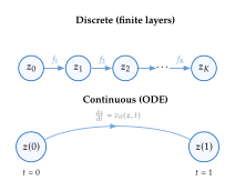
Rather than composing discrete layers, we can define a continuous transformation as the solution of an ordinary differential equation (ODE).

Definition 12 (Neural ODE).

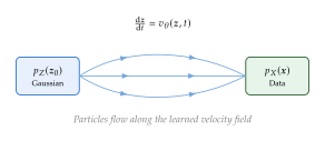
A neural ODE [6] defines a continuous transformation by (Neural ODE) $\begin{matrix} \frac{d 𝒛 (t)}{d t} = v_{θ} (𝒛 (t), t), 𝒛 (0) = 𝒛_{0}, \end{matrix}$ where $v_{θ} : ℝ^{D} \times [0,1] \to ℝ^{D}$ is a time-dependent velocity field parameterised by a neural network. The transformation $f_{θ} : 𝒛_{0} \mapsto 𝒛 (1)$ maps the initial condition to the solution at time $t = 1$ .

If $v_{θ}$ is Lipschitz continuous in $𝒛$ , then by the Picard–Lindelöf theorem the ODE has a unique solution for each initial condition, and the flow map $f_{θ}$ is a diffeomorphism. Crucially, the neural network $v_{θ}$ has no architectural constraints: it need not be triangular, coupling, or otherwise structured.

The instantaneous change of variables

Theorem 5 (Instantaneous change of variables).

Let $𝒛 (t)$ evolve according to $\frac{d 𝒛}{d t} = v_{θ} (𝒛 (t), t)$ . The log-density along the trajectory satisfies (INST COV) $\begin{matrix} \frac{d}{d t} \log p (𝒛 (t), t) = - trace (\frac{\partial v_{θ}}{\partial 𝒛} (𝒛 (t), t)) = - div v_{θ} (𝒛 (t), t) . \end{matrix}$

Proof.

The density $p (𝒛, t)$ satisfies the continuity equation (conservation of probability mass): $\frac{\partial p (𝒛, t)}{\partial t} + div (p (𝒛, t) v_{θ} (𝒛, t)) = 0.$ Expanding the divergence: $\frac{\partial p}{\partial t} + ⟨ \nabla_{𝒛} p, v_{θ} ⟩ + p \cdot div v_{θ} = 0.$ Now consider a particle trajectory $𝒛 (t)$ satisfying the ODE. The total time derivative of $\log p$ along this trajectory is $\begin{matrix} \frac{d}{d t} \log p (𝒛 (t), t) & = \frac{1}{p} (\frac{\partial p}{\partial t} + ⟨ \nabla_{𝒛} p, \frac{d 𝒛}{d t} ⟩) = \frac{1}{p} (\frac{\partial p}{\partial t} + ⟨ \nabla_{𝒛} p, v_{θ} ⟩) . \end{matrix}$ Substituting from the continuity equation: $\frac{d}{d t} \log p (𝒛 (t), t) = \frac{1}{p} (- p \cdot div v_{θ}) = - div v_{θ} = - trace (\frac{\partial v_{θ}}{\partial 𝒛}) .$

∎

Integrating (INST COV) from $t = 0$ to $t = 1$ gives (CNF LOGP) $\begin{matrix} \log p (𝒛 (1), 1) = \log p (𝒛 (0), 0) - \int_{0}^{1} trace (\frac{\partial v_{θ}}{\partial 𝒛} (𝒛 (t), t)) d t . \end{matrix}$

Key Idea.

The continuous change-of-variables formula replaces the $\log | \det 𝐉 |$ of discrete flows with an integral of the trace of the Jacobian (the divergence). Computing a trace is $𝒪 (D)$ instead of $𝒪 (D^{3})$ for a determinant, but we still need efficient estimation since the Jacobian itself costs $𝒪 (D^{2})$ to form.

Hutchinson's trace estimator

Definition 13 (Hutchinson's trace estimator).

For a matrix $𝐀 \in ℝ^{D \times D}$ , Hutchinson's estimator approximates the trace as (Hutchinson) $\begin{matrix} trace (𝐀) \approx 𝝐^{⊤} 𝐀 𝝐, \end{matrix}$ where $𝝐 \in ℝ^{D}$ is a random vector with $𝔼 [𝝐] = 0$ and $𝔼 [𝝐 𝝐^{⊤}] = 𝐈$ (e.g., $ϵ_{d} \overset{iid}{\sim} 𝒩 (0,1)$ or $ϵ_{d} \overset{iid}{\sim} Rademacher$ ).

Proposition 6 (Unbiasedness of Hutchinson's estimator).

The estimator $\hat{τ} = 𝝐^{⊤} 𝐀 𝝐$ satisfies $𝔼 [\hat{τ}] = trace (𝐀)$ .

Proof.

$𝔼 [𝝐^{⊤} 𝐀 𝝐] = 𝔼 [\sum_{i, j} ϵ_{i} A_{i j} ϵ_{j}] = \sum_{i, j} A_{i j} 𝔼 [ϵ_{i} ϵ_{j}] = \sum_{i, j} A_{i j} δ_{i j} = \sum_{i} A_{i i} = trace (𝐀) .$ The third equality uses $𝔼 [ϵ_{i} ϵ_{j}] = δ_{i j}$ .

∎

Remark 4.

The vector-Jacobian product $𝝐^{⊤} \frac{\partial v_{θ}}{\partial 𝒛}$ can be computed in $𝒪 (D)$ time using reverse-mode automatic differentiation, without forming the full Jacobian. This makes the trace estimation $𝒪 (D)$ per sample, compared to $𝒪 (D^{2})$ for the exact trace.

FFJORD

Definition 14 (FFJORD).

FFJORD (Free-Form Jacobian of Reversible Dynamics) [7] combines neural ODEs with Hutchinson's trace estimator. Training solves the augmented ODE (Ffjord) $\begin{matrix} \frac{d}{d t} (\begin{matrix} 𝒛 (t) \\ \log p (t) \end{matrix}) = (\begin{matrix} v_{θ} (𝒛 (t), t) \\ - 𝝐^{⊤} \frac{\partial v_{θ}}{\partial 𝒛} 𝝐 \end{matrix}), \end{matrix}$ from $t = 1$ (data) to $t = 0$ (base distribution), using an adaptive ODE solver (e.g., Dormand–Prince).

Algorithm 2 (FFJORD training step).

Input: Data point $𝒙$ , velocity network $v_{θ}$ , base density $p_{Z}$
Sample $𝝐 \sim 𝒩 (0, 𝐈)$
Solve ODE from $t = 1$ to $t = 0$ : $(𝒛_{0}, Δ \log p) = ODESolve ([𝒛, ℓ] \mapsto [v_{θ} (𝒛, t), - 𝝐^{⊤} \frac{\partial v_{θ}}{\partial 𝒛} 𝝐], [𝒙, 0], t : 1 \to 0)$
$\log p_{θ} (𝒙) = \log p_{Z} (𝒛_{0}) - Δ \log p$
$ℒ = - \log p_{θ} (𝒙)$ Negative log-likelihood
Update $θ$ via gradient descent on $ℒ$

Continuous normalizing flow: particles from the base distribution (Gaussian, left) flow along trajectories defined by the neural ODE to produce the data distribution (right).

Discrete flows (top) compose finitely many invertible layers. Continuous flows (bottom) define the transformation as the solution of an ODE, parameterised by a single velocity network evaluated at all times.

Flow Matching

FFJORD requires solving an ODE during training, which is slow and memory-intensive. Flow matching [8] provides a simulation-free alternative: instead of simulating trajectories, we directly regress the velocity field $v_{θ}$ onto a target velocity field that generates the desired probability path.

Definition 15 (Flow matching objective).

Given a probability path $p_{t}$ from a base distribution $p_{0}$ to the data distribution $p_{1}$ , with generating velocity field $u_{t}$ (i.e., $\partial_{t} p_{t} + div (p_{t} u_{t}) = 0$ ), the flow matching loss is (FM) $\begin{matrix} ℒ_{FM} (θ) = 𝔼_{t \sim 𝒰 [0,1]} 𝔼_{𝒛 \sim p_{t}} ‖ v_{θ} (𝒛, t) - u_{t} (𝒛) ‖^{2} . \end{matrix}$

The difficulty is that neither $p_{t}$ nor $u_{t}$ is known in closed form for complex data distributions. The breakthrough of Lipman et al. [8] (and independently Liu et al. [16]) is to work with conditional paths.

Theorem 6 (Conditional flow matching).

Let $p_{t} (𝒛 | 𝒙_{1})$ be a conditional probability path from $p_{0} = 𝒩 (0, 𝐈)$ to $p_{1} (\cdot | 𝒙_{1}) \approx δ_{𝒙_{1}}$ , with conditional velocity field $u_{t} (𝒛 | 𝒙_{1})$ . The conditional flow matching loss (CFM) $\begin{matrix} ℒ_{CFM} (θ) = 𝔼_{t \sim 𝒰 [0,1]} 𝔼_{𝒙_{1} \sim p_{data}} 𝔼_{𝒛 \sim p_{t} (\cdot | 𝒙_{1})} ‖ v_{θ} (𝒛, t) - u_{t} (𝒛 | 𝒙_{1}) ‖^{2} \end{matrix}$ has the same gradients as the (intractable) flow matching loss $ℒ_{FM}$ : $\nabla_{θ} ℒ_{CFM} = \nabla_{θ} ℒ_{FM}$ .

Proof.

Define the marginal velocity field as $u_{t} (𝒛) = 𝔼_{𝒙_{1} \sim p (𝒙_{1} | 𝒛, t)} [u_{t} (𝒛 | 𝒙_{1})]$ , which generates the marginal path $p_{t} (𝒛) = 𝔼_{𝒙_{1} \sim p_{data}} [p_{t} (𝒛 | 𝒙_{1})]$ .

Expand the CFM loss: $\begin{matrix} ℒ_{CFM} (θ) & = 𝔼_{t} 𝔼_{𝒙_{1}} 𝔼_{𝒛 \sim p_{t} (\cdot | 𝒙_{1})} [‖ v_{θ} (𝒛, t) ‖^{2} - 2 ⟨ v_{θ} (𝒛, t), u_{t} (𝒛 | 𝒙_{1}) ⟩ + ‖ u_{t} (𝒛 | 𝒙_{1}) ‖^{2}] . \end{matrix}$ The first term depends on $θ$ and can be rewritten as $𝔼_{𝒛 \sim p_{t}} ‖ v_{θ} (𝒛, t) ‖^{2}$ (marginalising over $𝒙_{1}$ ). The cross-term becomes $\begin{matrix} 𝔼_{𝒙_{1}} 𝔼_{𝒛 \sim p_{t} (\cdot | 𝒙_{1})} ⟨ v_{θ}, u_{t} (\cdot | 𝒙_{1}) ⟩ & = 𝔼_{𝒛 \sim p_{t}} ⟨ v_{θ} (𝒛, t), 𝔼_{𝒙_{1} \sim p (𝒙_{1} | 𝒛, t)} [u_{t} (𝒛 | 𝒙_{1})] ⟩ \\ = 𝔼_{𝒛 \sim p_{t}} ⟨ v_{θ} (𝒛, t), u_{t} (𝒛) ⟩, \end{matrix}$ which matches the cross-term of $ℒ_{FM}$ . Since the third term does not depend on $θ$ , the gradients are equal.

∎

Definition 16 (Optimal transport conditional path).

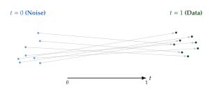
The simplest conditional path is the linear interpolation (or optimal transport path): (OT PATH) $\begin{matrix} 𝒛_{t} = (1 - t) 𝝐 + t 𝒙_{1}, 𝝐 \sim 𝒩 (0, 𝐈) . \end{matrix}$ The conditional velocity field is constant: $u_{t} (𝒛_{t} | 𝒙_{1}) = 𝒙_{1} - 𝝐$ . The CFM loss becomes (OT CFM) $\begin{matrix} ℒ_{O T - C F M} (θ) = 𝔼_{t, 𝒙_{1}, 𝝐} ‖ v_{θ} ((1 - t) 𝝐 + t 𝒙_{1}, t) - (𝒙_{1} - 𝝐) ‖^{2} . \end{matrix}$

Proposition 7 (Gaussian conditional paths).

For the Gaussian conditional path $p_{t} (𝒛 | 𝒙_{1}) = 𝒩 (𝒛; μ_{t} (𝒙_{1}), σ_{t}^{2} 𝐈)$ with $μ_{0} = 0$ , $σ_{0} = 1$ , $μ_{1} = 𝒙_{1}$ , $σ_{1} \approx 0$ , the conditional velocity field is $\begin{matrix} u_{t} (𝒛 | 𝒙_{1}) = \frac{{\dot{σ}}_{t}}{σ_{t}} (𝒛 - μ_{t} (𝒙_{1})) + {\dot{μ}}_{t} (𝒙_{1}), \end{matrix}$ where ${\dot{μ}}_{t}$ and ${\dot{σ}}_{t}$ denote time derivatives. For the OT path ( $μ_{t} = t 𝒙_{1}$ , $σ_{t} = 1 - t$ ), this simplifies to $u_{t} (𝒛 | 𝒙_{1}) = (𝒙_{1} - 𝒛) / (1 - t)$ .

Flow matching with OT conditional paths. Each noise sample

𝝐

(blue, left) is paired with a data sample

𝒙_{1}

(green, right), and the model learns the straight-line velocity

𝒙_{1} - 𝝐

. The velocity field

v_{θ}

is trained to predict these conditional velocities.

Insight.

Flow matching avoids ODE simulation during training entirely. The training loop is remarkably simple: (1) sample $t \sim 𝒰 [0,1]$ , $𝒙_{1} \sim p_{data}$ , $𝝐 \sim 𝒩 (0, 𝐈)$ ; (2) form $𝒛_{t} = (1 - t) 𝝐 + t 𝒙_{1}$ ; (3) regress $v_{θ} (𝒛_{t}, t)$ onto $𝒙_{1} - 𝝐$ . At inference, generate samples by solving the ODE $\frac{d 𝒛}{d t} = v_{θ} (𝒛, t)$ from $t = 0$ to $t = 1$ . This makes flow matching as simple to train as a denoising score matching objective, while producing a deterministic ODE sampler.

Remark 5 (Connection to diffusion models).

Flow matching is closely related to diffusion models (19). The “variance-preserving” path used in DDPMs corresponds to a Gaussian conditional path with $μ_{t} = \sqrt{{\overline{α}}_{t}} 𝒙_{1}$ and $σ_{t} = \sqrt{1 - {\overline{α}}_{t}}$ . The probability flow ODE of Song et al. [12] provides a deterministic sampler for diffusion models that is equivalent to a continuous normalizing flow. Flow matching can be viewed as a unified framework that encompasses both diffusion models and normalizing flows.

Connections and Applications

Flows for variational inference.

Rezende and Mohamed [2] originally proposed normalizing flows to improve the approximate posterior in VAEs (15). Instead of a simple Gaussian $q_{ϕ} (𝒛 | 𝒙) = 𝒩 (𝒛; 𝝁_{ϕ}, 𝚺_{ϕ})$ , one applies a flow to the Gaussian samples: $𝒛_{K} = f_{K} \circ \dots \circ f_{1} (𝒛_{0})$ , with $𝒛_{0} \sim q_{ϕ}$ . The ELBO is modified to include the flow's log-determinant terms. This yields a more flexible posterior that better approximates the true posterior, tightening the ELBO.

Optimal transport connection.

The OT conditional path in flow matching ((OT PATH)) is closely related to McCann's displacement interpolation in optimal transport (14). The linear interpolation $𝒛_{t} = (1 - t) 𝝐 + t 𝒙_{1}$ corresponds to the geodesic in Wasserstein space between the source and target distributions, when the coupling is the independent coupling.

Probability flow ODE.

Song et al. [12] showed that every stochastic diffusion process has an associated deterministic ODE, the probability flow ODE, that generates the same marginal distributions $p_{t}$ . This ODE defines a continuous normalizing flow, connecting diffusion models to the flow framework.

Modern applications.

Normalizing flows and flow matching underlie several state-of-the-art generative systems:

Image generation: Stable Diffusion 3 and Flux [13] use rectified flow (a flow matching variant) as the backbone.
Speech synthesis: Parallel WaveGAN and related models use flows for efficient audio generation.
Molecular generation: Flows on manifolds are used for drug design and protein structure prediction.
Density estimation: Neural spline flows remain state-of-the-art on tabular benchmarks.

Key Idea.

Normalizing flows, continuous flows, and flow matching form a progression: from discrete invertible layers with structured Jacobians, to continuous ODE-based transformations with free-form architectures, to simulation-free training of velocity fields. Each step trades architectural constraints for training simplicity, culminating in flow matching, a method as easy to train as denoising diffusion while retaining exact likelihoods (in principle) and deterministic sampling.

Architecture	Inverse	Log-det cost	Free arch.?	Key ref.
NICE / RealNVP	Analytic	$𝒪 (D)$	No	[3][4]
Glow	Analytic	$𝒪 (D + C)$	No	[5]
MAF	Sequential	$𝒪 (D)$	No	[9]
Neural spline	Analytic	$𝒪 (D K)$	No	[14]
iResNet	Fixed-point	$𝒪 (D)$ est.	Partial	[11]
FFJORD	ODE solve	$𝒪 (D)$ est.	Yes	[7]
Flow matching	ODE solve	N/A (train)	Yes	[8]

Comparison of normalizing flow architectures.

Exercises

Exercise 1 (1D change of variables).

Let $Z \sim 𝒩 (0, 1)$ and $X = \exp (Z)$ (so $X$ is log-normal). Using the change-of-variables formula, derive the density $p_{X} (x)$ and verify that it integrates to 1.

Exercise 2 (Coupling layer Jacobian).

For the affine coupling layer with $𝒛_{A} = (z_{1}, z_{2})$ , $𝒛_{B} = (z_{3}, z_{4})$ , and scale/translation networks $s (𝒛_{A}) = (s_{1}, s_{2})$ , $t (𝒛_{A}) = (t_{1}, t_{2})$ :

Write out the full $4 \times 4$ Jacobian matrix explicitly.
Compute its determinant and verify it equals $\exp (s_{1} + s_{2})$ .
Write the inverse transformation.

Exercise 3 (NICE is volume-preserving).

Prove that each additive coupling layer in NICE preserves volume, i.e., $| \det \frac{\partial 𝒙}{\partial 𝒛} | = 1$ . Explain why this implies that a NICE flow (without the final scaling layer) can only model distributions with the same total “volume” as the base distribution.

Exercise 4 (Composing coupling layers).

Show that a single affine coupling layer cannot represent the transformation $(z_{1}, z_{2}) \mapsto (z_{1} + z_{2}, z_{1} \cdot z_{2})$ . However, show that two coupling layers (with alternating partitions) can represent $(z_{1}, z_{2}) \mapsto (z_{1} + z_{2}, z_{2})$ .

Exercise 5 (LU decomposition cost).

For a $C \times C$ weight matrix in Glow's $1 \times 1$ convolution:

What is the cost of computing $\det 𝐖$ without the LU decomposition?
What is the cost with the LU decomposition?
For a $32 \times 32 \times C$ feature map, what is the total log-determinant contribution of one $1 \times 1$ convolution layer?

Exercise 6 (MAF density evaluation).

Consider a 3-dimensional MAF with affine transformations $x_{d} = z_{d} \exp (s_{d}) + t_{d}$ where: $s_{1} = 0, t_{1} = 0$ ; $s_{2} = 0.5 x_{1}, t_{2} = x_{1}$ ; $s_{3} = x_{1} + x_{2}, t_{3} = x_{1} x_{2}$ . For $𝒙 = (1, 2, 3)$ and base distribution $p_{Z} = 𝒩 (0, 𝐈)$ , compute $\log p_{X} (𝒙)$ .

Exercise 7 (MAF–IAF duality).

Starting from the MAF transformation $x_{d} = z_{d} \exp (s_{d} (𝒙_{< d})) + t_{d} (𝒙_{< d})$ , derive the inverse transformation and show it has the form of an IAF. Explain why density evaluation in MAF is $𝒪 (1)$ depth but sampling is $𝒪 (D)$ depth.

Exercise 8 (Hutchinson's estimator variance).

For a $D \times D$ matrix $𝐀$ and Rademacher random vector $𝝐$ ( $ϵ_{d} \in {- 1, + 1}$ with equal probability):

Prove that $𝔼 [𝝐^{⊤} 𝐀 𝝐] = trace (𝐀)$ .
Show that $𝖵ar [𝝐^{⊤} 𝐀 𝝐] = 2 ‖ 𝐀 ‖_{F}^{2} - 2 \sum_{i} A_{i i}^{2}$ when $𝐀$ is symmetric.
Explain why the variance is zero when $𝐀$ is diagonal.

Exercise 9 (Continuity equation derivation).

Derive the continuity equation $\frac{\partial p}{\partial t} + div (p v) = 0$ from conservation of probability mass. Hint: consider the total probability in an arbitrary region $Ω$ and use the divergence theorem.

Exercise 10 (Flow matching with Gaussian paths).

For the variance-preserving path $p_{t} (𝒛 | 𝒙_{1}) = 𝒩 (𝒛; \sqrt{{\overline{α}}_{t}} 𝒙_{1}, (1 - {\overline{α}}_{t}) 𝐈)$ :

Compute the conditional velocity field $u_{t} (𝒛 | 𝒙_{1})$ .
Write the resulting CFM loss.
Compare this with the denoising score matching objective of diffusion models.

Exercise 11 (Spline bijectivity).

For a rational-quadratic spline with $K = 2$ bins on $[- 1, 1]$ :

Write the spline function explicitly given bin widths $w_{1} = w_{2} = 1$ , bin heights $h_{1} = 0.5, h_{2} = 1.5$ , and boundary derivatives $d_{0} = d_{1} = d_{2} = 1$ .
Verify that $g (- 1) = - 1$ , $g (0) = - 0.5$ , $g (1) = 1$ .
Compute $g^{'} (0)$ and verify it is positive.

Exercise 12 (Residual flow convergence).

For $g (𝒛) = 0.5 \sin (𝒛)$ (applied element-wise) and $f (𝒛) = 𝒛 + g (𝒛)$ :

Verify that $Lip (g) = 0.5 < 1$ .
For $𝒙 = (1.5, 0)$ , run three iterations of the fixed-point inversion $𝒛^{(n + 1)} = 𝒙 - g (𝒛^{(n)})$ starting from $𝒛^{(0)} = 𝒙$ .
Estimate the convergence rate.

Exercise 13 (Flow vs VAE vs GAN).

Compare normalizing flows, VAEs, and GANs along the following axes:

Exact vs approximate likelihood computation.
Training stability.
Sample quality vs diversity trade-off.
Latent space structure and interpolation.

For each axis, explain which model family has the advantage and why.

Exercise 14 (Implementing a 2D RealNVP).

Describe (in pseudocode) a complete 2D RealNVP flow with: $K = 4$ affine coupling layers, alternating which dimension is transformed, and scale/translation networks as two-layer MLPs with 64 hidden units.

Write the forward pass (sampling).
Write the inverse pass (density evaluation).
Write the log-likelihood computation.
How many learnable parameters does your model have?

Exercise 15 (OT vs VP paths in flow matching).

Compare the OT path $𝒛_{t} = (1 - t) 𝝐 + t 𝒙_{1}$ with the VP path $𝒛_{t} = \sqrt{{\overline{α}}_{t}} 𝒙_{1} + \sqrt{1 - {\overline{α}}_{t}} 𝝐$ (where ${\overline{α}}_{t}$ is a decreasing schedule from 1 to 0).

Show that both paths satisfy $p_{0} \approx 𝒩 (0, 𝐈)$ and $p_{1} \approx δ_{𝒙_{1}}$ .
Compute the velocity for each path.
Which path produces straighter trajectories? Why does this matter for ODE solvers?

References

Density Estimation by Dual Ascent of the Log-Likelihood

Esteban G. Tabak, Eric Vanden-Eijnden

Communications in Mathematical Sciences, vol. 8, no. 1, pp. 217-233 · 2010

BibTeX

@article{tabak2010density,
  title={Density Estimation by Dual Ascent of the Log-Likelihood},
  author={Tabak, Esteban G. and Vanden-Eijnden, Eric},
  journal={Communications in Mathematical Sciences},
  volume={8},
  number={1},
  pages={217--233},
  year={2010}
}

Journal article

Variational Inference with Normalizing Flows

Danilo Jimenez Rezende, Shakir Mohamed

International Conference on Machine Learning, pp. 1530-1538 · 2015

BibTeX

@inproceedings{rezende2015variational,
  title={Variational Inference with Normalizing Flows},
  author={Rezende, Danilo Jimenez and Mohamed, Shakir},
  booktitle={International Conference on Machine Learning},
  pages={1530--1538},
  year={2015}
}

Conference paper

NICE: Non-linear Independent Components Estimation

Laurent Dinh, David Krueger, Yoshua Bengio

International Conference on Learning Representations (ICLR) Workshop · 2015

BibTeX

@inproceedings{dinh2015nice,
  title={{NICE}: Non-linear Independent Components Estimation},
  author={Dinh, Laurent and Krueger, David and Bengio, Yoshua},
  booktitle={International Conference on Learning Representations (ICLR) Workshop},
  year={2015}
}

Conference paper

Density estimation using Real NVP

Laurent Dinh, Jascha Sohl-Dickstein, Samy Bengio

International Conference on Learning Representations · 2017

BibTeX

@inproceedings{dinh2016density,
  title={Density estimation using Real NVP},
  author={Dinh, Laurent and Sohl-Dickstein, Jascha and Bengio, Samy},
  booktitle={International Conference on Learning Representations},
  year={2017}
}

Conference paper

Glow: Generative Flow with Invertible 1x1 Convolutions

Diederik P. Kingma, Prafulla Dhariwal

Advances in Neural Information Processing Systems, pp. 10236-10245 · 2018

BibTeX

@inproceedings{kingma2018glow,
  title={Glow: Generative Flow with Invertible 1x1 Convolutions},
  author={Kingma, Diederik P. and Dhariwal, Prafulla},
  booktitle={Advances in Neural Information Processing Systems},
  pages={10236--10245},
  year={2018}
}

Conference paper

Neural Ordinary Differential Equations

Ricky T. Q. Chen, Yulia Rubanova, Jesse Bettencourt, David K. Duvenaud

Advances in Neural Information Processing Systems · 2018

BibTeX

@inproceedings{chen2018neural,
  title={Neural Ordinary Differential Equations},
  author={Chen, Ricky T. Q. and Rubanova, Yulia and Bettencourt, Jesse and Duvenaud, David K.},
  booktitle={Advances in Neural Information Processing Systems},
  year={2018}
}

Conference paper

FFJORD: Free-form Continuous Dynamics for Scalable Reversible Generative Models

Will Grathwohl, Ricky T. Q. Chen, Jesse Bettencourt, Ilya Sutskever, David Duvenaud

International Conference on Learning Representations · 2019

BibTeX

@inproceedings{grathwohl2018ffjord,
  title={{FFJORD}: Free-form Continuous Dynamics for Scalable Reversible Generative Models},
  author={Grathwohl, Will and Chen, Ricky T. Q. and Bettencourt, Jesse and Sutskever, Ilya and Duvenaud, David},
  booktitle={International Conference on Learning Representations},
  year={2019}
}

Conference paper

Flow Matching for Generative Modeling

Yaron Lipman, Ricky T. Q. Chen, Heli Ben-Hamu, Maximilian Nickel, Matt Le

International Conference on Learning Representations (ICLR) · 2023

BibTeX

@inproceedings{lipman2023flow,
  title={Flow Matching for Generative Modeling},
  author={Lipman, Yaron and Chen, Ricky T. Q. and Ben-Hamu, Heli and Nickel, Maximilian and Le, Matt},
  booktitle={International Conference on Learning Representations (ICLR)},
  year={2023}
}

Conference paper

Masked Autoregressive Flow for Density Estimation

George Papamakarios, Theo Pavlakou, Iain Murray

Advances in Neural Information Processing Systems, pp. 2338-2347 · 2017

BibTeX

@inproceedings{papamakarios2017masked,
  title={Masked Autoregressive Flow for Density Estimation},
  author={Papamakarios, George and Pavlakou, Theo and Murray, Iain},
  booktitle={Advances in Neural Information Processing Systems},
  pages={2338--2347},
  year={2017}
}

Conference paper

Improved Variational Inference with Inverse Autoregressive Flow

Diederik P. Kingma, Tim Salimans, Rafal Jozefowicz, Xi Chen, Ilya Sutskever, Max Welling

Advances in Neural Information Processing Systems, pp. 4743-4751 · 2016

BibTeX

@inproceedings{kingma2016improved,
  title={Improved Variational Inference with Inverse Autoregressive Flow},
  author={Kingma, Diederik P. and Salimans, Tim and Jozefowicz, Rafal and Chen, Xi and Sutskever, Ilya and Welling, Max},
  booktitle={Advances in Neural Information Processing Systems},
  pages={4743--4751},
  year={2016}
}

Conference paper

Invertible Residual Networks

Jens Behrmann, Will Grathwohl, Ricky T. Q. Chen, David Duvenaud, Jorn-Henrik Jacobsen

Proceedings of the 36th International Conference on Machine Learning (ICML) · 2019

BibTeX

@inproceedings{behrmann2019invertible,
  title={Invertible Residual Networks},
  author={Behrmann, Jens and Grathwohl, Will and Chen, Ricky T. Q. and Duvenaud, David and Jacobsen, J\"{o}rn-Henrik},
  booktitle={Proceedings of the 36th International Conference on Machine Learning (ICML)},
  year={2019}
}

Conference paper

Score-Based Generative Modeling through Stochastic Differential Equations

Yang Song, Jascha Sohl-Dickstein, Diederik P. Kingma, Abhishek Kumar, Stefano Ermon, Ben Poole

Proceedings of ICLR · 2021

BibTeX

@article{song2021scorebased,
  author    = {Song, Yang and Sohl-Dickstein, Jascha and Kingma, Diederik P. and Kumar, Abhishek and Ermon, Stefano and Poole, Ben},
  title     = {Score-Based Generative Modeling through Stochastic Differential Equations},
  journal   = {Proceedings of ICLR},
  year      = {2021}
}

Journal article

Scaling Rectified Flow Transformers for High-Resolution Image Synthesis

Patrick Esser, Sumith Kulal, Andreas Blattmann, Rahim Entezari, Jonas Muller, Harry Saini, Yam Levi, Dominik Lorber, et al.

Proceedings of the 41st International Conference on Machine Learning (ICML) · 2024

BibTeX

@inproceedings{esser2024scaling,
  title={Scaling Rectified Flow Transformers for High-Resolution Image Synthesis},
  author={Esser, Patrick and Kulal, Sumith and Blattmann, Andreas and Entezari, Rahim and M\"{u}ller, Jonas and Saini, Harry and Levi, Yam and Lorber, Dominik and Sauer, Axel and Boesel, Frederic and others},
  booktitle={Proceedings of the 41st International Conference on Machine Learning (ICML)},
  year={2024}
}

Conference paper

Neural Spline Flows

Conor Durkan, Artur Bekasov, Iain Murray, George Papamakarios

Advances in Neural Information Processing Systems (NeurIPS) · 2019

BibTeX

@inproceedings{durkan2019neural,
  title={Neural Spline Flows},
  author={Durkan, Conor and Bekasov, Artur and Murray, Iain and Papamakarios, George},
  booktitle={Advances in Neural Information Processing Systems (NeurIPS)},
  year={2019}
}

Conference paper

Residual Flows for Invertible Generative Modeling

Ricky T. Q. Chen, Jens Behrmann, David K. Duvenaud, Jorn-Henrik Jacobsen

Advances in Neural Information Processing Systems (NeurIPS) · 2019

BibTeX

@inproceedings{chen2019residual,
  title={Residual Flows for Invertible Generative Modeling},
  author={Chen, Ricky T. Q. and Behrmann, Jens and Duvenaud, David K. and Jacobsen, J\"{o}rn-Henrik},
  booktitle={Advances in Neural Information Processing Systems (NeurIPS)},
  year={2019}
}

Conference paper

Flow Straight and Fast: Learning to Generate and Transfer Data with Rectified Flow

Xingchao Liu, Chengyue Gong, Qiang Liu

International Conference on Learning Representations (ICLR) · 2023

BibTeX

@inproceedings{liu2023flow,
  title={Flow Straight and Fast: Learning to Generate and Transfer Data with Rectified Flow},
  author={Liu, Xingchao and Gong, Chengyue and Liu, Qiang},
  booktitle={International Conference on Learning Representations (ICLR)},
  year={2023}
}

Conference paper

← 17 Autoregressive Models 19 Diffusion Models →

18 Normalizing Flows

Change of Variables and Flow Foundations

The change-of-variables formula

Composing flows

Triangular maps and the Knothe–Rosenblatt rearrangement

Coupling Flows: NICE and RealNVP

NICE

RealNVP and multi-scale architecture

Glow and Invertible 1×1 Convolutions

Autoregressive Flows: MAF and IAF

Neural Spline Flows

Residual Flows

Log-determinant estimation.

Continuous Normalizing Flows

Neural ordinary differential equations

The instantaneous change of variables

Hutchinson's trace estimator

FFJORD

Flow Matching

Connections and Applications

Flows for variational inference.

Optimal transport connection.

Probability flow ODE.

Modern applications.

Exercises

References

Glow and Invertible $1 \times 1$ Convolutions