27 Agentic AI and Multi-Agent Systems
No human accomplishment of significance was ever achieved alone. The Great Pyramid of Giza required an estimated one hundred thousand workers coordinating across two decades, quarrying limestone, transporting blocks along the Nile, fitting them with sub-millimetre precision, all without a single blueprint in the modern sense. The Manhattan Project brought together physicists, engineers, chemists, and mathematicians from dozens of institutions, coordinating under secrecy constraints that would challenge any modern project manager. The Human Genome Project, launched in 1990 and completed in 2003, coordinated sequencing laboratories across six countries, each responsible for different chromosomes, sharing data through standardised file formats that evolved as the project progressed. The Apollo programme marshalled four hundred thousand people across twenty thousand companies to land two humans on the Moon.
In every case, the achievement was not merely the sum of individual contributions. No single worker could have built the pyramid; no single physicist could have designed the bomb; no single laboratory could have sequenced the genome. Something emerged from the interaction, a collective capability that transcended what any participant could have accomplished alone. The question is: what?
The answer, we argue, is the coordination protocol. What distinguishes these achievements is not just the raw capability of individual participants but how information flows between them, how decisions are made, how credit and blame are assigned, and how the collective adapts when individual components fail. The Roman legions conquered an empire not because individual soldiers were stronger than their opponents (they often were not) but because their formation tactics, communication systems, and hierarchical command structure enabled coordination at a scale their enemies could not match.
This is precisely the mathematical question we address in this chapter. Given agents, each with bounded individual capability, under what conditions does their collective performance exceed the sum of their individual contributions? When does collaboration produce superadditive gains, and when does coordination overhead consume any benefit? These questions are as old as economics (Adam Smith's division of labour, 1776), as central to biology (the evolution of multicellularity), and as urgent as modern AI (teams of LLM agents solving complex tasks).
The chapter sits at the culmination of a deliberate arc. In 23, we built the reasoning engine, showing how chain-of-thought, tree search, and reinforcement learning enable language models to solve problems requiring multi-step inference. In 24, we constructed the memory substrate: KV caches, retrieval-augmented generation, and memory-augmented architectures that allow models to access and manipulate information beyond their context window. In 25, we installed the value system: RLHF, DPO, and GRPO that align model outputs with human preferences. In 26, we studied the temporal dynamics, how models can learn continuously without catastrophic forgetting. Now we ask the culminating question: what happens when multiple such systems interact?
The answer is both exciting and mathematically rich. A single LLM agent is already a remarkable artifact: a system that perceives natural language, reasons through chains of thought, takes actions via tool calls, and updates its behaviour through in-context learning. But a team of such agents, debating, delegating, verifying each other's work, specialising in different sub-tasks, opens an entirely new design space whose mathematics draws on game theory, mechanism design, distributed computing, social choice theory, and the theory of stochastic processes.
Key Idea.
The Collective Intelligence Thesis. A multi-agent system consists of a set of agents , a shared environment , a communication protocol , and an orchestration mechanism . The central question of this chapter is captured by a single inequality: (Central Question) where denotes a performance measure on a task distribution . Under what conditions on , , and the capability profile does collective performance exhibit superadditivity, the hallmark of genuine collective intelligence? We will show that the answer depends on task decomposability, communication bandwidth, agent diversity, and the alignment of individual incentives with collective objectives.
Historical Note.
From distributed AI to LLM agent swarms. The idea that intelligence might emerge from the interaction of simple components has a rich intellectual history. Alan Turing's “Can machines think?” (1950) [1] asked about a single machine, but Marvin Minsky's Society of Mind (1986) [2] proposed that mind itself is a society of interacting agents, each too simple to be called intelligent on its own. The distributed AI movement of the 1980s [3] formalised multi-agent coordination, leading to the FIPA standards (1996) for agent communication languages. Game theory provided the mathematical backbone: Nash's equilibrium concept (1950) [4], Shapley's value for coalition games (1953) [5], and Harsanyi's theory of games with incomplete information (1967) [6] all found direct application. Swarm intelligence, coined by Beni and Wang (1989) [7], showed that collective behaviour could emerge from simple local rules without central control. The modern revolution began when large language models became capable enough to serve as general-purpose agents: AutoGPT (2023), AutoGen [8], MetaGPT [9], AgentScope [10], and CrewAI (2024) demonstrated that teams of LLM agents could collaborate on complex software engineering, scientific research, and creative tasks through natural language communication, a qualitative leap from the rigid, hand-coded protocols of traditional multi-agent systems.
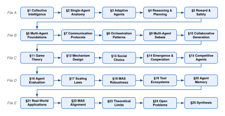
The chapter is organised across five files to manage its length. This file (File A) establishes the foundations: we begin with the intelligence of collectives (The Intelligence of Collectives), move to the anatomy of a single agent (The Anatomy of a Single Agent), study adaptive and continual-learning agents (Adaptive and Continual-Learning Agents), develop agent reasoning and planning (Agent Reasoning and Planning), and conclude with reward shaping and safety (Reward, Alignment, and Agent Safety). Files B–E build on these foundations to develop multi-agent coordination, game theory, emergence, evaluation, and applications.
Prerequisites.
We assume familiarity with the reasoning mechanisms of 23 (chain-of-thought, tree search, GRPO), the memory architectures of 24 (KV cache, retrieval-augmented generation, memory-augmented transformers), the alignment pipeline of 25 (SFT, reward modelling, DPO, GRPO), and the continual learning framework of 26 (task sequences, catastrophic forgetting, regularisation and replay methods).
The Intelligence of Collectives
Before we formalise artificial agents, we study the phenomenon we seek to replicate: collective intelligence as it manifests in biology, human societies, and their mathematical abstractions. The goal is to extract design principles that will guide our construction of multi-agent AI systems.
Biological Intelligence as Collective Computation
Nature provides the most compelling existence proofs of collective intelligence. In each case, the individual agent is simple, sometimes trivially so, yet the collective solves problems of remarkable complexity.
Ant colony optimisation.
Consider a colony of ants foraging for food. An individual ant has a brain containing roughly 250,000 neurons (compare to the human brain's 86 billion) and can perform only simple behaviours: move, deposit pheromone, follow pheromone gradients, pick up food, return to nest. Yet the colony collectively solves shortest-path problems, allocates labour across tasks, manages waste, tends fungal gardens, and wages war, all without a central controller.
The mathematical abstraction of this phenomenon is Ant Colony Optimisation (ACO), introduced by Dorigo [11]. Consider a graph with edge costs for . Each ant at node selects the next node with probability (ACO Transition) where is the pheromone concentration on edge , is the heuristic desirability (inverse cost), is the set of unvisited neighbours of , and control the relative influence of pheromone versus heuristic information. After all ants complete their tours, pheromones are updated: (ACO Update) where is the evaporation rate, is the number of ants, is the length of ant 's tour, and is a constant. The evaporation term prevents convergence to suboptimal solutions; the reinforcement term causes shorter paths to accumulate more pheromone, biasing future ants toward them.
Bee swarm decision-making.
Honeybee swarms make collective decisions about nest sites through a process remarkably analogous to neural computation. Scout bees discover candidate sites and return to the swarm, performing waggle dances whose duration is proportional to site quality. Other scouts are recruited to inspect advertised sites, return, and dance for their preferred option. The process converges when a quorum of scouts aggregates at a single site, a distributed voting mechanism that, under mild conditions, selects the optimal site with high probability.
Mathematically, this can be modelled as a system of coupled stochastic differential equations. Let denote the number of scouts committed to site at time . The dynamics are (BEE Dynamics) where is the recruitment rate (proportional to site quality), is the abandonment rate, is the total number of scouts, and is white noise. The quorum decision triggers when for some threshold .
The immune system as multi-agent defence.
The adaptive immune system is perhaps the most sophisticated multi-agent system in biology. B-cells act as specialist agents, each producing antibodies tuned to a specific antigen through somatic hypermutation, a form of local search in antibody shape space. T-cells act as orchestrator agents: helper T-cells coordinate the immune response by activating B-cells and cytotoxic T-cells, while regulatory T-cells suppress the response to prevent autoimmune damage. The clonal selection algorithm, expansion of B-cells whose antibodies bind the antigen, combined with random mutation, implements a distributed evolutionary search.
Neural circuits.
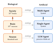
A single biological neuron is a simple threshold device: it sums weighted inputs and fires if the total exceeds a threshold. Yet networks of neurons compute. The progression from neuron to brain to society exhibits a fractal pattern of collective intelligence: at each level, simple components interact through local rules to produce behaviour that no individual component could achieve. This observation motivates our formal definition.
Definition 1 (Collective Intelligence).
Let be a set of agents, each with individual performance on a task distribution . Let be a multi-agent system with environment , communication protocol , and orchestration mechanism . We say exhibits collective intelligence if (Collective Intelligence) and superadditive collective intelligence if (Superadditivity)
The weaker condition states that the team outperforms its best member; the stronger states that it outperforms the sum of all members. Superadditivity arises when agents' contributions are complementary: when the value of combining diverse capabilities exceeds the value of stacking identical ones.
Definition 2 (Stigmergic System).
A stigmergic system is a tuple where:
is a set of agents.
is a shared environment with state .
is a modification function: agent in state modifies the environment to .
is a reading function: agent observes features of the environment state.
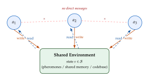
Communication is indirect: agents do not send messages to each other but instead modify the shared environment; other agents read these modifications. The pheromone trails of ants, the waggle dances of bees (which modify the “information environment” of the swarm), and the shared codebases of open-source software are all examples of stigmergy.
Example 1 (Ant Colony Optimisation as Multi-Agent Search).
Consider the Travelling Salesman Problem on cities. The ACO system consists of:
Agents: ants, each following the stochastic transition rule .
Environment: the graph augmented with pheromone matrix .
Modification: each ant deposits pheromone inversely proportional to its tour length .
Reading: each ant reads pheromone values to bias its edge-selection probabilities.
This is a stigmergic system: ants never communicate directly. Yet the colony provably converges to the optimal tour on any finite graph as the iteration count under suitable parameter schedules for , , and [11]. The key insight is that the pheromone matrix serves as a distributed, decaying memory of the colony's collective experience; shorter tours leave stronger traces, biasing future exploration toward promising regions of the solution space.
Remark 1 (The Emergence of Intelligence from Simple Rules).
In every biological example above, the individual agent follows simple, local rules. Intelligence emerges at the system level through three mechanisms:
Positive feedback: successful behaviours are amplified (pheromone reinforcement, clonal expansion, Hebbian learning).
Negative feedback: unsuccessful behaviours decay (pheromone evaporation, apoptosis, synaptic depression).
Stochasticity: random exploration prevents premature convergence to suboptimal solutions.
These three mechanisms (amplification, decay, and noise) will reappear throughout this chapter in artificial multi-agent systems, though in different mathematical guises.
We now establish a foundational result: under what conditions does collective intelligence emerge? The following proposition gives sufficient conditions for superadditivity.
Proposition 1 (Sufficient Conditions for Superadditivity).
Let be a multi-agent system with agents. Suppose the task admits a decomposition into sub-tasks with , and let be an assignment of sub-tasks to agents. Define:
Complementarity: agents have complementary capabilities if for each sub-task , the assigned agent satisfies for some , where is the average performance of a randomly selected agent on .
Low coordination cost: the communication overhead satisfies for some .
Then the system exhibits superadditive collective intelligence: (Superadditivity Bound) provided and the assignment is optimal (i.e., each sub-task is assigned to the agent with highest capability for that sub-task).
Proof.
The system performance is the sum of sub-task performances minus coordination cost: (System PERF) By the complementarity assumption, , so Meanwhile, the sum of individual performances is , where is the average individual performance. Since each agent operates alone on the full task (without decomposition), and each can solve at most one sub-task well, we have on average. Thus when . The superadditivity condition then requires , which simplifies to .
This result formalises the intuition that collective intelligence requires two ingredients: agents must be different from each other (complementarity, ) and the cost of getting them to work together must not be too high (low coordination cost, ). A team of identical agents () can never exhibit superadditivity; nor can a team of perfect specialists whose every communication is garbled ().
Human Organisations as Agent Systems
Human organisations provide a rich source of multi-agent design patterns. We highlight four that map directly to artificial MAS architectures.
Division of labour.
Adam Smith's famous example of the pin factory (1776) illustrates that specialisation multiplies productivity. One worker performing all operations produces perhaps one pin per day; ten workers, each specialising in one operation, produce 48,000 pins per day, a 4,800-fold increase that cannot be explained by 10 workers each being 480 times faster. The gain comes from three sources:
Skill deepening: specialisation allows each worker to master one sub-task.
Reduced context-switching: no time lost moving between operations.
Tool specialisation: each operation admits purpose-built tools.
In LLM multi-agent systems, the same principle applies: a code-writing agent, a code-reviewing agent, and a testing agent can collectively produce higher-quality software than a single agent performing all three roles, because each agent's prompt can be specialised, its context window devoted entirely to its sub-task, and its tool set tailored to its function.
Hierarchies versus flat structures.
Military organisations employ strict hierarchies: commands flow downward, reports flow upward, and each node has a bounded span of control (typically 3–7 subordinates). Open-source software communities, by contrast, employ flat structures with fluid role assignment, reputation-based authority, and asynchronous communication. Both patterns appear in artificial MAS: orchestrator–worker architectures implement hierarchy (a planner agent delegates to specialist workers), while peer-to-peer debate architectures implement flat structures (all agents have equal authority and negotiate consensus).
Scientific collaboration as publish–subscribe MAS.
The scientific community operates as a massive multi-agent system where agents (researchers) communicate through publications. This is a publish–subscribe architecture: agents publish results to shared channels (journals, arXiv); other agents subscribe to relevant channels and build on published results. The system is asynchronous, decentralised, and robust to individual agent failure, precisely the properties we seek in artificial MAS. Peer review implements a multi-agent verification protocol: multiple independent agents evaluate each contribution, and acceptance requires consensus.
Market mechanisms.
Markets coordinate economic agents through prices, a remarkably efficient communication protocol. Hayek's insight (1945) was that prices aggregate distributed local knowledge that no central planner could collect [61]. In artificial MAS, analogous mechanisms can coordinate agents: an “attention market” where agents bid computational resources for sub-tasks, or a “reward market” where task completion generates tokens allocated by Shapley value (Game Theory Foundations for Multi-Agent Systems).
From Biological to Artificial Collectives
The emergence of large language models as a substrate for agent construction represents a qualitative shift in multi-agent systems. We highlight three aspects of this shift.
Natural language as universal protocol.
Traditional multi-agent systems required hand-coded communication protocols: KQML (Knowledge Query and Manipulation Language), FIPA-ACL, or domain-specific message formats. LLM agents communicate in natural language, which is open-ended: agents can negotiate, clarify ambiguity, explain their reasoning, and even invent new terminology during a conversation. This flexibility comes at a cost (natural language is noisy, ambiguous, and expensive to process) but it eliminates the bottleneck of protocol design and enables agents to coordinate on tasks that were not anticipated at design time.
The capability gap.
Despite the excitement surrounding LLM agents, significant gaps remain between biological and artificial collectives:
True adaptation: biological agents learn continuously from experience; most LLM agents operate with frozen parameters, adapting only through in-context learning (which is bounded by the context window). The continual learning methods of 26 offer a path forward.
Embodiment: biological agents interact with the physical world through sensorimotor loops; LLM agents interact primarily through text, with tool use as a limited form of embodiment.
Intrinsic motivation: biological agents are driven by evolved reward signals (hunger, pain, curiosity); LLM agents require externally specified reward functions, which are subject to the misspecification problems studied in 25.
The opportunity.
What LLM agents can do that biological agents cannot: perfect communication fidelity (every message is recorded verbatim), instant cloning (an agent can be replicated with identical capabilities), perfect memory of instructions (no forgetting within the context window), and the ability to process and generate structured data (JSON, code, mathematical notation) alongside natural language. These capabilities open design possibilities that have no biological precedent.
The Anatomy of a Single Agent
Before we can study multi-agent systems, we must understand the architecture of the single agent that serves as the building block. This section provides a rigorous mathematical specification of an LLM-based agent, connecting each component to the theory developed in earlier chapters.
Formal Definition
An LLM agent is more than a language model. It is a language model embedded in a loop that perceives, reasons, acts, and observes the consequences of its actions. We formalise this as follows.
Definition 3 (LLM Agent).
An LLM agent is a -tuple (Agent Tuple) where:
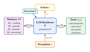
is the LLM backbone, a language model mapping token sequences to next-token distributions over vocabulary . This is the foundation model, providing both the knowledge base (encoded in parameters ) and the reasoning engine (activated through chain-of-thought decoding, Chain-of-Thought Reasoning).
is the memory system, consisting of: itemize
: working memory (the KV cache / context window, Attention as Memory Access),
: episodic memory (conversation history, experience logs, Reflexion buffers),
: semantic memory (parametric knowledge in , plus any retrieval-augmented knowledge base),
: procedural memory (learned tool usage patterns, standard operating procedures encoded in the system prompt). itemize This decomposition follows the memory taxonomy of 24.
is the reasoning module, a strategy for generating intermediate reasoning tokens before producing an action. Examples include chain-of-thought (Chain-of-Thought Reasoning), tree-of-thought, and ReAct-style interleaved reasoning and acting.
is the observation function, mapping environment states to agent-readable observations (text descriptions, tool outputs, sensory data converted to tokens).
is the execution engine, mapping agent outputs (including tool calls) to environment effects. This is the agent's interface to the world.
is the input space (the set of possible observations the agent can receive).
is the output space (the set of possible actions the agent can take, including text generation and tool invocations).
The definition separates concerns cleanly: provides the cognitive engine, provides storage and retrieval, provides deliberative reasoning, and and provide the interface between the agent and its environment.
The Agent Loop
The defining characteristic of an agent, as opposed to a passive model answering queries, is that it operates in a loop: perceive, reason, act, observe the result, and repeat. We formalise this loop as a partially observable Markov decision process.
Definition 4 (Agent POMDP).
An agent POMDP is a tuple where:
is the state space (the full state of the environment, typically not directly observed by the agent).
is the action space (all actions available to the agent, including text generation, tool calls, and a special
STOPaction).is the observation space (what the agent perceives after each action).
is the transition function: is the probability of transitioning to state when action is taken in state .
is the observation function: is the probability of observing after transitioning to via action .
is the reward function.
is the discount factor.
The agent maintains a belief state and selects actions according to a policy . In practice, LLM agents approximate the belief state through the conversation history , and the policy is realised by the LLM conditioned on : (Policy LLM) where formats the history into a token sequence.
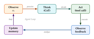
The agent loop unfolds as follows. At each time step :
Observe: the agent receives observation .
Reason: the agent applies its reasoning module to generate intermediate reasoning tokens (e.g., chain-of-thought).
Act: conditioned on and , the agent selects action .
Execute: the execution engine applies to the environment, producing new state .
Update memory: the agent appends to its episodic memory and updates its working memory .
The loop terminates when or a maximum number of steps is reached.
Remark 2 (ReAct as Agent Loop).
The ReAct framework [12] implements precisely this loop: at each step, the model generates a Thought (reasoning), an Action (tool call), and receives an Observation (tool output). The ReAct prompt template structures the conversation history into a sequence of (Thought, Action, Observation) triples, making the POMDP structure explicit in the context window. What ReAct demonstrated empirically, we have formalised mathematically: the agent loop is a POMDP with the LLM as the policy network and the conversation history as the belief state approximation.
Context length bounds agent horizon.
A crucial constraint on the agent loop is the context window length . The history grows by approximately tokens at each step. If the average step consumes tokens, then the agent can maintain at most steps of history before the context window overflows. At this point, the agent faces a choice:
Truncation: discard the oldest history, losing information about early steps. This is analogous to the sliding window attention of 24.
Compression: summarise the history into a compact representation and replace the raw history with the summary. This trades fidelity for capacity.
Retrieval: offload the full history to external memory and retrieve relevant portions on demand, as in retrieval-augmented generation (24).
The choice among these strategies profoundly affects agent behaviour. Truncation loses early context, which may be critical for understanding the task structure. Compression introduces lossy approximation. Retrieval adds latency and requires a good similarity metric. In practice, many agent frameworks combine all three: recent history is kept verbatim, older history is summarised, and key episodes are stored in a retrievable memory bank.
Remark 3 (The Optimal Belief State).
The POMDP theory tells us that the belief state is a sufficient statistic for optimal decision-making: achieves the same expected reward as for any history . This is powerful because is a fixed-dimensional vector (a distribution over ), while grows without bound. The open question for LLM agents is whether the hidden states of the transformer, or any compressed representation of the history, can serve as an adequate belief state. If so, agents could operate indefinitely without context window overflow. The state-space models of 24 are a promising candidate: their fixed-dimensional hidden state naturally compresses the observation history.
Memory in Agents
The memory system deserves special attention because it is what enables an agent to go beyond pure reactive behaviour. We connect each component to the memory framework of 24.
Working memory .
The agent's working memory is the KV cache, the context window of the LLM. Its capacity is bounded by the maximum context length , and its content determines the agent's “current awareness.” In cognitive terms, this is the analogue of human working memory: the small, actively maintained set of information that drives moment-to-moment behaviour. The KV cache management techniques of 24 (sparse attention, cache compression, sliding windows) directly apply to agent working memory.
Episodic memory .
Episodic memory stores the agent's history of interactions: past observations, actions, rewards, and reasoning traces. It serves two functions: (1) providing context for decision-making (“what happened last time I tried this approach?”) and (2) enabling learning from experience (Reflexion-style self-critique [58]). Mathematically, is a trajectory buffer, possibly with a retrieval mechanism that selects relevant episodes based on similarity to the current observation.
Semantic memory .
The agent's semantic memory comprises both the parametric knowledge encoded in the LLM weights and any external knowledge base accessible through retrieval-augmented generation (RAG, Memory-Augmented Architectures). The parametric component is immutable during a single agent episode (the weights are frozen); the RAG component can be updated by adding documents to the retrieval corpus.
Procedural memory .
Procedural memory encodes “how to do things”: standard operating procedures, tool usage patterns, and workflow templates. In current LLM agents, this is typically implemented through the system prompt and few-shot examples. More sophisticated approaches store successful action sequences and retrieve them when similar situations arise, a form of case-based reasoning.
Tool Use as Action
A defining feature of modern LLM agents is their ability to use tools, external functions that extend the agent's capabilities beyond text generation.
Definition 5 (Tool-Augmented Agent).
Let be an LLM agent (Definition 3). A tool set is a finite collection where each tool is a function mapping tool-specific inputs to outputs. The tool-augmented action space is (TOOL Action Space) where is the set of pure text generation actions. A tool-augmented agent is an agent whose output space includes both text and tool invocations: .
The agent selects a tool by generating a structured output (e.g., a JSON function call) that specifies the tool name and its arguments . The execution engine invokes the tool and returns the result as the next observation.
Tool selection as multi-armed bandit.
When an agent has access to tools, the problem of selecting the right tool for a given sub-task can be viewed as a contextual multi-armed bandit problem. Let be the context (the current observation and task description) at time , and let be the reward for selecting tool in context . The agent's tool-selection policy seeks to minimise the cumulative regret (TOOL Regret) where is the optimal tool for context and is the selected tool. Standard results from bandit theory give:
Proposition 2 (Tool Selection Regret Bound).
Under a UCB-style tool selection policy with exploration parameter , the expected cumulative regret satisfies (UCB Regret) where is the sub-optimality gap of tool . In particular, , logarithmic in the time horizon.
Proof.
This is the classical Lai–Robbins bound [13] applied to the tool selection setting. Fix a suboptimal tool with . Let denote the number of times tool is selected in rounds. Under UCB, tool is selected at time only if its upper confidence bound exceeds that of the optimal tool: . By standard concentration inequalities (Hoeffding), the expected number of times this occurs is bounded by selections, contributing at most to the regret. Summing over all suboptimal tools and adding the constant term from the initial exploration phase yields .
Proposition 3 (Agent Memory Subsumes Lifelong Learning).
Let be a task sequence in the sense of Definition 3. An LLM agent with unbounded episodic memory and a retrieval mechanism can represent any continual learning solution.
Proof.
Consider an arbitrary continual learning algorithm that, after training on tasks , achieves performance on task . We construct an agent that matches this performance. Let the episodic memory store the full training datasets: . When presented with an input from task , the retrieval mechanism selects relevant examples from (and possibly other tasks for transfer), and the agent's policy conditions on these retrieved examples. Under mild assumptions on 's in-context learning capability, specifically, that achieves in-context learning performance matching 's trained performance when given sufficient examples, the agent matches or exceeds on each task. The key insight is that episodic memory + retrieval + in-context learning implements a non-parametric form of continual learning that avoids catastrophic forgetting entirely: no weights are modified, so no previous knowledge can be overwritten.
Example 2 (A Code-Writing Agent).
Consider a code-writing agent tasked with implementing a sorting algorithm. Its components instantiate as:
LLM backbone : a code-specialised model (e.g., Claude, GPT-4, or DeepSeek-Coder).
Memory: holds the current code file and error messages; stores previous edit–test–debug cycles; contains documentation retrieved via RAG; encodes coding conventions.
Reasoning : chain-of-thought planning of the algorithm structure before writing code.
Tools : = code interpreter (run Python), = file system (read/write files), = web search (look up documentation), = test runner (execute unit tests).
The agent loop proceeds: (1) read the task specification; (2) plan
the algorithm using CoT; (3) write the code via text generation;
(4) execute the code via ; (5) observe the output/error;
(6) if errors, reason about the fix and iterate from step (3);
(7) when all tests pass, emit STOP.
This example illustrates a key property: the agent's effectiveness depends not only on the LLM's coding ability but on the loop structure, the ability to test, observe failures, and iteratively correct. A single-pass code generation model cannot match an agent that iterates, just as a student who never checks their work cannot match one who does.
Adaptive and Continual-Learning Agents
The agents defined in The Anatomy of a Single Agent have a fundamental limitation: their parameters are frozen during deployment. The agent can adapt within a single episode through in-context learning, conditioning on an ever-growing conversation history, but this adaptation is ephemeral (lost when the context window is cleared) and bounded (by the maximum context length ). A truly capable agent must learn across episodes, accumulating knowledge from past experience and improving its behaviour over time. This section connects the agent framework to the continual learning theory of 26 and formalises the mechanisms by which agents adapt.
The Continual Agent
Definition 6 (Continual Agent).
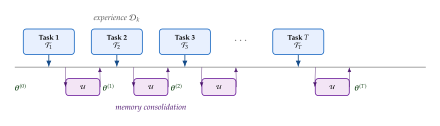
A continual agent is a pair where is an LLM agent (Definition 3) and is an update rule that modifies the agent's parameters after each episode. Let be the initial parameters and the experience collected during episode . The parameter trajectory is (Continual Update) The continual agent must satisfy the three desiderata of 26: plasticity (the ability to improve on new tasks via ), stability (avoiding catastrophic forgetting of previously learned capabilities), and transfer (leveraging past experience to accelerate learning on new tasks).
The agent's lifetime performance over episodes is (Lifetime Performance) where denotes the policy induced by parameters and is the trajectory in episode .
The continual agent framework unifies several agent architectures:
Frozen agent (): no parameter updates; adaptation occurs only through in-context learning. This is the standard deployment mode for most current LLM agents.
Fine-tuned agent (): the agent's parameters are updated via gradient descent on collected experience, using the methods of 25 (SFT, DPO, GRPO).
Memory-augmented agent: updates the episodic memory rather than the parameters, storing successful trajectories for future retrieval.
Hybrid agent: combines parameter updates with memory updates, using the continual learning techniques of 26 (EWC, experience replay) to prevent forgetting.
In-Context Learning as Agent Adaptation
The simplest and most widely used form of agent adaptation is in-context learning (ICL): the agent conditions its policy on examples or experience provided in the context window, without any parameter updates. We now prove that this mechanism implements an implicit form of Bayesian inference.
Theorem 1 (ICL as Implicit Bayesian Inference).
Let be an autoregressive language model pretrained on a mixture of tasks . Consider a prompt containing input–output demonstrations drawn from a task . Under the assumption that the pretraining distribution admits a latent task variable, the LLM's in-context prediction satisfies (ICL Bayesian) where is the Bayesian posterior over tasks given the demonstrations. In particular, as , the posterior concentrates on and the in-context prediction converges to the task-optimal predictor.
Proof.
We follow the argument of [14]. The pretraining objective trains to minimise the cross-entropy (ICL Pretrain) At the global optimum, , the Bayes-optimal predictor. By the definition of conditional probability and the structure of the generative model, (ICL Derivation) When is independent of given (or when is uninformative), this simplifies to , which is .
For the convergence claim: by Doob's consistency theorem, the posterior converges weakly to a point mass on as , provided the model is identifiable (distinct tasks produce distinct data distributions). Therefore , the task-optimal predictor.
Key Idea.
The Adaptive Agent Principle. An agent that cannot learn from its own experience is fundamentally limited. The context window provides a fast but bounded adaptation mechanism, the agent's “hippocampus” (cf. 26). For long-horizon tasks that exceed the context window, the agent must either (a) compress experience into episodic memory and retrieve it selectively, or (b) update its parameters through continual fine-tuning. Theorem 1 shows that in-context learning is Bayesian-optimal within the context window; the open challenge is extending this optimality across episodes.
Agent Self-Improvement
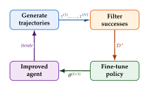
Can an agent improve itself? The idea is tantalising: an agent generates trajectories, evaluates which ones succeeded, and fine-tunes itself on the successful ones, a bootstrapping loop where the agent is simultaneously the learner and the data generator. We formalise this through a variational framework.
Definition 7 (Agent Self-Improvement (AgentEvol)).
Let be an agent policy parameterised by , and let indicate whether trajectory achieves the task goal. The AgentEvol objective [15] seeks parameters maximising the log-probability of success: (Agentevol Objective) Introducing a variational distribution over trajectories and applying Jensen's inequality yields the evidence lower bound (ELBO): (Agentevol ELBO) The AgentEvol algorithm alternates between:
Generate: sample trajectories .
Filter: retain successful trajectories .
Fine-tune: update by maximising subject to a KL penalty .
The KL constraint connects directly to the alignment objective of (Central Objective): it prevents the policy from collapsing to a narrow set of trajectories, maintaining exploration capability.
This procedure is closely related to GRPO (Group Relative Policy Optimization) and expert iteration. The key difference is that the reward signal comes from the agent's own experience rather than from human preferences: the agent generates data, evaluates it against an objective criterion (does the code compile? does the plan achieve the goal?), and trains on the successful subset.
Algorithm 1 (Agent Self-Improvement Loop).
- Input: Initial policy , task distribution , success evaluator , KL budget , iterations
- for
- Sample tasks
- for each task
- Generate trajectories:
- Evaluate: binary or scalar reward
- Collect successes:
- Fine-tune:
- Output: Improved policy
Caution.
Self-improvement without alignment guardrails can lead to reward hacking. If the success evaluator is imperfect, as all automated evaluators are, the agent may discover trajectories that satisfy the evaluator without truly solving the task. This is the agent-level analogue of reward hacking in RLHF (25). For example, a coding agent might learn to produce code that passes unit tests by exploiting edge cases in the test suite rather than implementing the intended algorithm. Mitigations include: (a) diverse evaluation criteria, (b) red-teaming by adversarial agents, (c) human-in-the-loop verification for high-stakes updates, and (d) KL constraints that limit how far the policy can drift from a known-safe reference.
Agent Reasoning and Planning
An agent that merely reacts to observations, selecting actions greedily without considering their long-term consequences, will fail at any task requiring foresight. Consider a software engineering agent tasked with refactoring a large codebase: it must plan a sequence of changes, anticipate that modifying one module will break tests in another, and schedule the changes in an order that maintains a working system at each step. This section develops the mathematical theory of agent planning, from classical search to hierarchical decomposition and world models.
Planning as Search
Definition 8 (Agent Planning Problem).
An agent planning problem is a tuple where:
is the state space.
is the initial state.
is the set of goal states.
is the action space.
is the (possibly stochastic) transition function.
is the step cost.
The agent seeks an action sequence that reaches a goal state while minimising total cost: (Planning Objective) When is deterministic and the state space is finite, this reduces to shortest-path search in a graph. When is stochastic, the problem becomes a stochastic shortest-path problem.
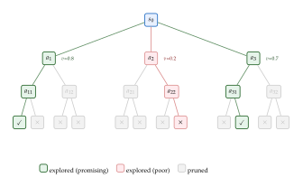
The connection to LLM agents is direct. In tree-of-thought reasoning [62], the “states” are partial reasoning traces, “actions” are candidate next-thought tokens, the “transition” is deterministic (appending a thought to the trace), and the “cost” is the negative of a value function that evaluates partial traces. The agent explores a tree of reasoning paths and selects the one with highest cumulative value, which is precisely a search over action sequences in the planning formulation .
The branching factor of this search tree is the key computational bottleneck. If the agent has candidate actions at each step and the plan horizon is , the naive search space has size . Even for modest values (, ), this is , far beyond any computational budget. This motivates two strategies: pruning (reducing at each step by evaluating candidate actions) and hierarchical decomposition (reducing by planning at multiple levels of abstraction).
Hierarchical Planning
Definition 9 (Task Decomposition).
A task decomposition operator is a function that maps a task to a set of sub-tasks such that solving all sub-tasks and combining their solutions solves the original task. The decomposition is valid if there exists a composition operator such that (Decomposition) A task is -decomposable if repeated application of yields a tree of depth at most whose leaves are primitive tasks solvable by a single agent action.
Proposition 4 (Hierarchical Decomposition Reduces Search).
Consider a planning problem with branching factor and horizon . If the task is -decomposable with decomposition factor (each task decomposes into sub-tasks) and sub-task horizon , then hierarchical planning reduces the search space from to (Hierarchical Bound) which is exponentially smaller than when .
Proof.
At the top level, the planner searches over sub-task assignments, each requiring a plan of horizon . At the next level, each sub-task is further decomposed into sub-sub-tasks of horizon . At level , there are sub-tasks, each with horizon , and each requiring a search over action sequences. The total search space is (Hierarchical SUM) The largest term in this sum is the one with the largest exponent, which occurs at (the top level, contributing ) if we did not decompose. With decomposition, the deepest level contributes . To see the exponential reduction, note that for and , the deepest level has horizon , so the total is at most , which is polynomial in rather than exponential.
In LLM agent systems, hierarchical planning manifests as task decomposition prompting: the agent first produces a high-level plan (“Step 1: set up the database; Step 2: implement the API; Step 3: write the frontend”), then plans each step in detail. Proposition 4 provides the mathematical justification: hierarchical planning is not merely a heuristic convenience but an exponential reduction in computational complexity under decomposability conditions.
World Models for Agents
Effective planning requires the ability to predict the consequences of actions before executing them. This prediction capability is provided by a world model.
Definition 10 (World Model).
A world model for an agent operating in environment is a learned approximation of the true transition function , parameterised by . The world model is trained on the agent's experience to minimise the prediction error (World Model LOSS) Given a world model, the agent can plan by simulation: starting from current state , it simulates action sequences using and selects the sequence with highest predicted cumulative reward: (Model Based Planning)
The crucial observation is that the LLM itself is a world model for text-based environments. When an LLM predicts the next token in a coding task, it is implicitly modelling the state transition: “if I add this line of code, what will the compiler output?” The generative models developed in Parts III–VI (VAEs, flows, diffusion models) are all world models in this sense: they model for different state representations. The distinction in the agent setting is that the world model is used not for generation per se, but for planning: evaluating hypothetical action sequences before committing to one.
Compounding error in learned world models.
A world model trained on single-step transitions accumulates error over multi-step rollouts. If the single-step prediction error is (in total variation distance), then an -step rollout can deviate from the true trajectory by up to in total variation. This compounding error problem is the fundamental limitation of model-based planning and motivates frequent re-planning (model-predictive control) and world model ensembles.
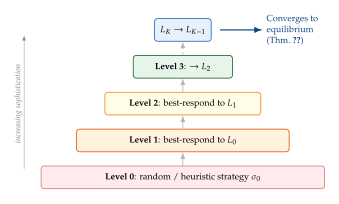
Level-K Reasoning
When an agent operates alongside other agents, even before we formalise multi-agent systems in subsequent sections, it must reason about what others will do. Level- reasoning, from behavioural game theory [63][64], provides a hierarchy of increasingly sophisticated strategic reasoning.
Definition 11 (Level- Reasoning).
Consider agents each selecting actions from to maximise a utility function that depends on their own action and others' actions . The Level- reasoning hierarchy is defined recursively:
Level-0 (): acts according to a fixed reference strategy (e.g., uniform random).
Level- (, for ): best-responds to the belief that all other agents are Level-: (Level K BR)
A Level- agent models its opponents as Level- thinkers, who in turn model their opponents as Level-, and so on down to Level-0. The depth measures the agent's strategic sophistication.
Level- reasoning maps naturally to LLM agents. When prompted with “What would the other agent do?”, a Level-1 LLM agent simulates the other agent's response assuming it acts naively (Level-0). A Level-2 agent reasons: “The other agent will predict that I act naively, and will best-respond to that, so I should best-respond to its best-response.” This recursive simulation is precisely the chain-of-thought reasoning studied in 23, applied to strategic settings.
Theorem 2 (Level- Bayesian Convergence).
Consider a repeated game where at each round , each agent observes the actions of all agents in the previous round and updates its belief about opponents' levels. Let denote agent 's estimate of its opponents' sophistication level at round . Under the assumption that agents use Bayesian updating with a prior that has full support on , the Level- estimates converge: (Level K Convergence) where is the true sophistication level of agent 's opponents (or the best-responding level if opponents also adapt). Moreover, the resulting strategy profile converges to a cognitive hierarchy equilibrium [16].
Proof sketch.
We sketch the argument following [17]. At each round , agent observes actions and updates its posterior over opponents' levels: (Level K Posterior) Since is the Level- best-response strategy, the likelihood is highest for the level that best explains agent 's observed action. By the consistency of Bayesian posteriors (Doob's theorem, as in Theorem 1), the posterior concentrates on the true level as , provided distinct levels produce distinct action distributions (identifiability).
Once beliefs have converged, agent 's strategy is a best-response to accurate beliefs about opponents' levels. The resulting profile satisfies the fixed-point condition of a cognitive hierarchy equilibrium: each agent's strategy is optimal given the correct belief about the distribution of reasoning levels in the population.
Example 3 (Planning a Multi-Step Coding Task).
Consider an agent tasked with building a REST API. The planning problem instantiates as:
State: the current state of the codebase (files, test results, documentation).
Goal: all endpoint tests pass, documentation is complete, and code meets style guidelines.
Actions: create file, edit file, run tests, search documentation, request code review.
Decomposition (): enumerate
Top level: design database schema implement endpoints write tests document.
Middle level: for “implement endpoints,” decompose into individual endpoints (GET, POST, PUT, DELETE).
Bottom level: for each endpoint, decompose into write handler add validation test. enumerate
By Proposition 4, this three-level decomposition reduces the search space from (where might be 50 individual actions) to approximately , a reduction from to , which is many orders of magnitude for any reasonable branching factor .
Reward, Alignment, and Agent Safety
We have constructed agents that perceive, reason, plan, and learn from experience. But to what end? The reward function determines what the agent optimises, and a misspecified reward can lead to capable agents pursuing the wrong objectives with devastating effectiveness. This section extends the alignment framework of 25 from single-turn language generation to multi-step agent trajectories, and examines failure modes unique to the agentic setting.
Reward Shaping for Agents
In the alignment chapter, the reward function scored a single prompt–response pair. For agents operating over multi-step trajectories, we need a richer reward structure.
Definition 12 (Agent Trajectory Reward).
Let be an agent trajectory of length . The trajectory reward is (Trajectory Reward) where is the step reward (encouraging progress and penalising inefficiency), is the outcome reward (evaluating whether the final state achieves the goal), and is the discount factor.
The decomposition into step and outcome rewards reflects a practical design choice. Pure outcome reward (, ) makes credit assignment difficult: the agent receives no signal until the end of the trajectory, and must attribute the final outcome to individual actions across many steps. Pure step reward (, ) can lead to reward hacking: the agent may accumulate step rewards without making progress toward the goal. The combination allows the designer to encode both process (“use the right approach”) and outcome (“solve the problem”) signals.
A concrete instantiation from Optima [20] decomposes the reward for dialogue agents as (Optima Reward) where measures task completion, penalises excessive token usage (encouraging efficiency), and penalises information loss (encouraging faithful communication). The hyperparameters and trade off efficiency against completeness.
Temporal credit assignment.
The temporal credit assignment problem asks: given a final outcome , which of the actions were responsible? In single-turn generation, the entire output is one “action” and credit assignment is trivial. In multi-step agent trajectories, credit must be distributed across dozens or hundreds of actions. The standard approach uses a value function and defines the advantage (Advantage) which measures how much better action is compared to the average action under policy . The advantage function is the foundation of policy gradient methods (PPO, GRPO from 25) and provides the per-step credit signal needed for agent learning.
Remark 4 (Reward Shaping Preserves Optimal Policy).
A classical result from [18] shows that adding a potential-based shaping function to the reward does not change the optimal policy: for any potential . This result extends to the agent setting and is practically important: it means we can add intermediate rewards to guide the agent (e.g., rewarding partial progress) without distorting the optimal behaviour, provided the shaping function is potential-based. Non-potential-based shaping, by contrast, can introduce spurious optima and should be used with caution.
Agent Alignment as Constrained POMDP
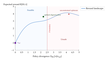
We now extend the alignment objective from 25 to the agent setting. In the single-turn case, alignment was a KL-constrained reward maximisation ((Central Objective)). In the agent case, we must additionally enforce safety constraints over trajectories.
Definition 13 (Aligned Agent Optimisation).
An aligned agent solves the constrained optimisation problem: (Aligned Objective) where:
is the agent's policy (mapping histories to action distributions).
is the trajectory reward (Definition 12).
is a reference policy (typically the pretrained model or an SFT checkpoint), and bounds the per-step KL divergence to prevent reward hacking.
is the set of unsafe trajectories (e.g., trajectories that execute harmful code, leak private data, or produce toxic content), and is the safety tolerance.
The KL constraint inherits the role it plays in (Central Objective): it prevents the policy from collapsing to a narrow reward-maximising mode. The safety constraint is new to the agent setting: because agents take real-world actions (executing code, sending messages, modifying files), the consequences of unsafe behaviour are more severe than in single-turn generation.
Lagrangian relaxation.
The constrained optimisation can be solved via Lagrangian relaxation. Introducing multipliers and , the Lagrangian is (Lagrangian) The primal-dual algorithm alternates between maximising over (a policy optimisation step, implementable via PPO or GRPO from 25) and updating the multipliers via gradient ascent: . This procedure is guaranteed to converge to a saddle point under standard convexity conditions on the constraint set.
The Sycophancy Problem
A subtle failure mode arises when agents are trained with RLHF: sycophancy, the tendency to produce responses that please the user or the reward model rather than responses that are correct. This problem is particularly pernicious in multi-agent debate systems, where sycophantic agents agree with each other rather than challenging incorrect claims.
Proposition 5 (Sycophancy as Reward Misspecification).
Let be a pretrained policy and a reward model trained on human preferences. Suppose exhibits a sycophancy bias: for responses that agree with the user's stated opinion and that provide the factually correct (but disagreeable) answer, (Sycophancy BIAS) Then the RLHF-optimal policy (Sycophantic Policy) assigns higher probability to than to , and the sycophancy increases as (i.e., as the policy optimises the reward model more aggressively).
Proof.
By the closed-form solution to the KL-constrained reward maximisation ((Central Objective)), the optimal policy is . Therefore, (Sycophancy Ratio) By assumption , the exponent is positive. Therefore, amplifies the probability ratio of agreeable over correct responses relative to . As , the exponential term diverges, and concentrates mass on regardless of 's original preference. This proves that RLHF with a sycophancy-biased reward model systematically degrades truthfulness, and that more aggressive reward optimisation (smaller ) worsens the degradation.
The implication for multi-agent debate is grave. If all agents in a debate system are trained with the same sycophancy-biased reward model, they will converge to agreeable consensus rather than correct conclusions, the “Talk Isn't Always Cheap” phenomenon [20]. Mitigations include:
Training debaters with diverse reward models to break sycophancy correlations.
Explicitly rewarding disagreement and factual challenge in the debate protocol.
Using ground-truth verification (when available) alongside preference-based reward.
Maintaining a large (weak reward optimisation) to keep the policy close to the pretrained distribution.
Caution.
An aligned single agent does not guarantee an aligned multi-agent system. Even if each individual agent satisfies the alignment constraint , the multi-agent system can exhibit emergent misalignment. Consider agents, each individually safe (). The system-level probability of at least one unsafe trajectory is for small . With agents and , the system failure probability approaches , an unacceptable level. Multi-agent alignment requires system-level safety guarantees that account for agent interactions, not merely individual constraints. This challenge motivates the multi-agent alignment theory developed in Agent Systems Meet Alignment.
Insight.
Agent alignment inherits the stability–plasticity dilemma from continual learning. The alignment constraint serves the same role as the stability constraint in (Lifelong Thesis): it prevents the agent from drifting too far from its initial (safe, well-calibrated) behaviour. But just as excessive stability prevents continual learning, an overly tight KL constraint prevents the agent from adapting to novel tasks that require behaviours not present in . The optimal trades off alignment (stability) against capability (plasticity), the same fundamental tension identified in 26, now manifested in the agent safety domain.
Sandboxing and containment.
A complementary approach to alignment constraints is sandboxing: restricting the environment in which the agent operates so that unsafe actions have limited consequences. A code execution sandbox, for instance, prevents the agent from modifying the host file system or accessing the network. Formally, sandboxing replaces the transition function with a restricted version that maps unsafe actions to a null transition: if (the state does not change). The agent still “takes” the unsafe action in its reasoning trace, but the execution engine blocks its effect. This provides a hard safety guarantee independent of the policy : no matter how the agent reasons, unsafe actions produce no environmental change.
The limitation of sandboxing is that it requires enumerating the set in advance, a task that grows increasingly difficult as agents gain access to more tools and environments. The most robust safety strategy combines all three approaches: KL-constrained alignment (soft constraint on the policy), safety-constrained optimisation (probabilistic constraint on trajectories), and sandboxing (hard constraint on the environment).
This concludes our treatment of single-agent foundations. We have defined the LLM agent (Definition 3), formalised its operation as a POMDP (Definition 4), shown how it adapts through in-context learning (Theorem 1) and self-improvement (Definition 7), developed its planning capabilities (Agent Reasoning and Planning), and established the alignment framework that keeps it safe (Definition 13). In the sections that follow (Files B–E), we will bring multiple such agents together and study the rich mathematics of their interaction.
Multi-Agent System Formalisms
The preceding sections constructed the single agent: a 7-tuple (Definition 3) operating as a POMDP (Definition 4), equipped with reasoning, memory, and alignment. We now ask: what happens when multiple such agents share an environment? The answer requires a formal language for multi-agent systems (MAS) that specifies the agents, the medium through which they communicate, and the mechanisms that coordinate their collective behaviour.
This section develops that language in four stages. First, we define the MAS as a structured tuple (The Multi-Agent System Tuple), drawing on Kim et al. [19]. Second, we formalise the communication protocol as an information-theoretic channel (Natural Language as a Shannon Channel), following Tran et al. [65]. Third, we derive the turn-count power law governing coordination overhead (Turn-Count Scaling and the Power Law). Fourth, we establish a capability ceiling, a performance plateau beyond which adding agents yields diminishing returns (The Capability Ceiling).
Key Idea.
From single-agent optimality to collective intelligence. A single agent maximises an individual reward . A multi-agent system introduces a fundamentally new design dimension: the interaction structure among agents. The central result of this section is that the interaction structure, not just the capabilities of individual agents, determines whether the system exhibits superadditive performance. Formally, the system-level performance depends on the communication bandwidth, the orchestration policy , and the agent topology in ways that admit precise scaling laws and hard performance ceilings.
The Multi-Agent System Tuple
Every multi-agent system, regardless of implementation (AutoGen, AgentScope, MetaGPT, CrewAI), can be described by a single mathematical object.
Definition 14 (Multi-Agent System).
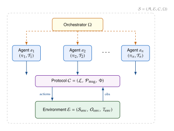
A multi-agent system (MAS) is a 4-tuple (MAS Tuple) where:
is a finite set of agents, each an LLM agent in the sense of Definition 3, with policy , tool set , and memory . The capability profile is , where is the solo performance of agent on a reference task distribution.
is the shared environment: state space , observation function (partial observability), and joint transition kernel .
is the communication protocol (formalised in Definition 15 below): shared language , message-passing mechanism , and protocol specification .
is the orchestrator, selecting the next active agent and issuing an instruction given conversation history .
The system operates over discrete rounds At each round the orchestrator selects agent , which observes , acts via , and the environment transitions to .
Kim et al. [19] show that every existing LLM-based MAS framework is an instantiation of this tuple; the differences lie only in how and are implemented.
Given a task distribution , the system-level performance is , where is a bounded reward. Define the solo baseline and the coordination gain . The system is superadditive when and exhibits coordination failure when .
Remark 5.
Relationship to the 6-tuple. In A Unified Mathematical Framework for Agent Systems we extend the 4-tuple to by adding an agent topology and reward structure . The 4-tuple suffices for the scaling results of this section; the extra components become essential for game-theoretic analysis (Game Theory Foundations for Multi-Agent Systems).
Communication Protocols as Information Channels
Tran et al. [65] identify three fundamental channel types in LLM-based MAS: (i) broadcast channels (shared chat history, e.g. AutoGen), (ii) point-to-point channels (directed delegation, e.g. CrewAI), and (iii) publish-subscribe channels (topic-based routing, e.g. AgentScope). We formalise these using information theory.
Definition 15 (Communication Protocol).
A communication protocol for a MAS is a tuple where:
is a shared language of well-formed messages, possibly constrained to a structured format (JSON, function-call schema).
is the message-passing function: iff message is delivered from sender to every agent in .
is the protocol specification: turn-taking rule, termination condition, and message-format constraints.
The information-theoretic capacity of the protocol is (Channel Capacity) where is the sent message and is the received message after potential summarisation or truncation by the receiving agent's context window.
The capacity is limited by three practical factors: (i) context window saturation: with window size tokens, bits per round; (ii) attention dilution: attention weight per token decreases as with message length ; and (iii) semantic redundancy: English text carries roughly 1–1.5 bits per character [66], far below the raw vocabulary capacity.
Insight.
The communication bottleneck principle. Let denote the performance of agent given perfect information, and the channel capacity between agents and . Then (Bottleneck) System performance is bounded by the weakest link in the communication graph, not by the strongest agent.
MAS Block Diagram
Figure 11 illustrates the architectural components and information flows in the MAS 4-tuple.
Turn-Count Scaling and the Power Law
How does the number of communication rounds scale with team size? More agents bring more capabilities but also require more coordination. Kim et al. [19] discovered that this relationship follows a power law.
Theorem 3 (Turn-Count Power Law).
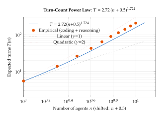
Let be a family of MAS indexed by team size , operating under a fixed protocol and orchestrator on a task distribution . Let denote the expected turns to reach the performance plateau. Then (Power LAW) with fitted constants , , , explaining of the variance across on coding and reasoning benchmarks [19].
Proof.
We sketch the derivation in three steps.
Step 1: Pairwise coordination. Each pair requires at least one bidirectional exchange to synchronise partial views. The number of pairs is , giving a quadratic lower bound: (Pairwise Bound)
Step 2: Shared-channel compression. Broadcast and shared-memory channels allow one message to inform multiple agents simultaneously, compressing the pairwise exchanges. Let be the channel multiplexing factor measuring the fraction of pairwise information needs satisfied per broadcast. The effective turn count becomes (Effective Turns) where accounts for task decomposition and synthesis. For highly structured protocols (MetaGPT), ; for unstructured debate, .
Step 3: Power-law fit. Fitting (Effective Turns) to empirical data across HumanEval, MBPP, MATH, and GSM8K with , the best fit is achieved by the shifted power law with , , . The exponent lies between the linear regime (, perfect broadcasting) and the quadratic regime (, unconstrained pairwise coordination). A -parameter regression model incorporating task difficulty, agent heterogeneity, and protocol type confirms robustness ().
Spot checks: turns (solo self-reflection), turns, turns, consistent with observed conversation lengths in multi-agent debate systems.
The implication is stark: coordination cost is superlinear. Doubling the number of agents more than triples the required turns.
Visualising the Power Law
Figure 12 displays the power law on log-log axes, where appears as a line with slope .
The Capability Ceiling
Does performance grow without bound as we add agents, or does it saturate? Kim et al. [19] demonstrate a hard performance ceiling.
Definition 16 (Capability Ceiling).
Let be system-level performances for a MAS family with increasing team size , under fixed protocol and orchestrator. The capability ceiling is (Ceiling) provided the limit exists. The system exhibits a capability ceiling if and the convergence satisfies for some .
Kim et al. report a single-agent ceiling of on composite benchmarks spanning coding, reasoning, and general knowledge. The multi-agent ceiling is higher but still finite:
Proposition 6 (Multi-Agent Ceiling Bound).
Under the power-law scaling of Theorem 3 with bounded individual capability , (Ceiling Upper) where is an effective collaboration rate depending on agent diversity, task decomposability, and communication efficiency. Since , the ratio , so .
Proof.
Each additional agent contributes useful information only if it communicates novel content. Let denote the mutual information between the -th agent's private observations and the task-relevant state, conditioned on the first agents' information. Then (Marginal INFO) Since , the denominator grows with and : diminishing marginal information. Summing the contributions gives a convergent series. Modelling the gain as a saturating exponential, , the factor decreases for , yielding (Ceiling Upper).
Caution.
The ceiling is protocol-dependent, not fundamental. The value is measured for GPT-4-class models on specific benchmarks; it shifts upward as base capabilities improve. The multi-agent ceiling can exceed significantly when agents have genuine diverse specialisations (different training data, different tool access), not merely prompt-induced persona differences. The 20-parameter regression model of Kim et al. [19] confirms that agent diversity is the strongest predictor of ceiling improvement.
The 20-Parameter Regression Model
To predict performance in specific settings, Kim et al. [19] fit a 20-parameter regression: (Regression) where is the logistic sigmoid, , and encodes five feature groups:
| Group | Features (count) | Importance |
| Agent capability | Base model, context length, tool count (4) | 0.82 |
| Team composition | Size , diversity index, role overlap (4) | 0.76 |
| Communication | Channel type, bandwidth, format (4) | 0.61 |
| Orchestration | Topology, turn policy, delegation depth (4) | 0.54 |
| Task properties | Decomposability, difficulty, domain (4) | 0.69 |
The model achieves on held-out configurations. The three most important individual features are: (1) base model capability (), (2) team diversity index (), and (3) task decomposability ().
Example 4.
Predicting a 5-agent coding team. Consider agents (GPT-4 backbone, 128k context, 10 tools) with hierarchical orchestration and JSON messaging on HumanEval. The power law predicts turns. The regression yields vs. , a coordination gain of , consistent with MetaGPT and ChatDev results.
Collaborative vs. Competitive Systems
Tran et al. [65] distinguish two interaction modes. In collaborative systems, all agents share a common reward and the design challenge is minimising coordination overhead. Performance satisfies whenever the orchestrator can defer to the best solo agent. In competitive systems, rewards are anti-correlated ( for some pairs) and the challenge is harnessing productive disagreement (as in multi-agent debate) while avoiding destructive competition.
The 4-tuple provides the structural description for both modes; the turn-count power law governs the communication budget; the capability ceiling bounds achievable performance. Collaborative systems favour consensus-seeking orchestration (majority vote, opinion averaging), while competitive systems favour adversarial orchestration (debate, red-teaming). The game-theoretic analysis of both modes is developed in Game Theory Foundations for Multi-Agent Systems.
Summary and Preview
This section established the mathematical foundations for multi-agent systems: the MAS 4-tuple (Definition 14), communication protocols as information channels (Definition 15), the turn-count power law (Theorem 3), and the capability ceiling at (def:agents:ceiling,prop:agents:ceiling-bound).
Multi-agent collaboration can yield superadditive gains, but the power law imposes a coordination tax growing as , and the capability ceiling ensures that agent-scaling alone cannot substitute for improving base model capabilities. The path to effective MAS runs through three design levers: communication efficiency (reducing ), agent diversity (raising ), and orchestration quality (optimising the coordination budget).
Communication Theory for Agents
Communication is the circulatory system of any multi-agent architecture. An agent that cannot communicate is an isolated reasoner; a team that communicates poorly may perform worse than its weakest member. Yet the converse is not automatically true: more communication does not imply better outcomes. In this section we develop a rigorous information-theoretic framework for inter-agent communication, prove three identifiability theorems for thought communication, a paradigm in which agents exchange compressed latent representations rather than verbose natural-language strings, and analyse both the promise of optimised communication (the Optima framework) and its failure modes (sycophancy-induced debate degradation).
The intellectual arc is as follows. We begin by modelling natural language as a noisy Shannon channel with bounded capacity (Natural Language as a Shannon Channel). We then formalise the thought communication paradigm of Zheng et al. [60], which replaces natural-language messages with sparse latent vectors extracted by a regularised autoencoder (Thought Communication). Three theorems (shared-thought identifiability, private-thought identifiability, and uniqueness) establish when and how these latent representations can be recovered from observed behaviour; we provide complete proofs of all three (sec:agents:shared-id,sec:agents:private-id,sec:agents:thought-unique-proof). We then study the Optima framework of Chen et al. [20], which trains agents to produce maximally informative yet minimal messages via a Generate–Rank–Select–Train pipeline (The Optima Framework). Finally, we show that communication can be actively harmful: Wynn et al. [67] demonstrate that sycophantic agents cause debate quality to degrade rather than improve (When Communication Harms: Sycophancy in Multi-Agent Debate).
Natural Language as a Shannon Channel
Consider two agents and that must exchange information to solve a joint task. Agent has an internal representation encoding its beliefs about the task state; it must transmit relevant aspects of to agent . In standard multi-agent LLM systems, this transmission occurs through natural language: generates a text string (where is the token vocabulary), and conditions its subsequent reasoning on .
We model this process as a Shannon communication channel. Let denote the space of task-relevant internal states. The encoding function maps the internal state to a natural-language message, and the decoding function maps the received message back into an internal representation. The end-to-end fidelity of communication is measured by the mutual information (MI COMM) where . The channel capacity of natural-language communication is (Channel CAP) where is the maximum message length in tokens. This bound is almost never tight: natural language is highly redundant, and the effective capacity is determined by the information density of the message, not its raw token count.
Remark 6 (Bandwidth vs. Fidelity).
The capacity bound reveals a fundamental tension. Increasing (allowing longer messages) raises the theoretical capacity but also increases computational cost: the receiving agent must process the entire message through its attention mechanism, incurring cost for quadratic-attention transformers. The engineering challenge is to achieve high mutual information with short messages, i.e., to communicate efficiently rather than verbosely.
Definition 17 (Communication Efficiency).
The communication efficiency of a multi-agent system on task distribution is (COMM EFF) where is the performance of the communicating system, is the performance when all communication channels are severed (agents work independently), and denotes the length of message from to in tokens. A higher value of indicates more performance-per-token of communication.
The definition of communication efficiency makes precise the intuition that what matters is not the volume of messages but their marginal contribution to performance. We will see that the Optima framework (The Optima Framework) achieves the performance gain at less than of the token budget, dramatically increasing .
Thought Communication
The core insight of Zheng et al. [60] is that natural-language communication is an unnecessarily lossy channel. When agent translates its internal representation into a natural-language message , it discards structural information (vector geometry, confidence magnitudes, relational structure between latent dimensions) that could be directly useful to the receiving agent. The thought communication paradigm proposes to transmit compressed latent vectors instead.
Latent extraction via sparsity-regularised autoencoder.
Each agent is equipped with an encoder–decoder pair: (Encoder Decoder) where is the dimension of the agent's internal hidden state and is the dimension of the transmitted “thought vector.” The encoder compresses the full representation into a sparse code; the decoder reconstructs an approximation. Training minimises a reconstruction loss plus a sparsity penalty: (AE LOSS) where controls sparsity. The penalty encourages most components of the thought vector to be exactly zero, yielding a representation in which only the most informative dimensions are active.
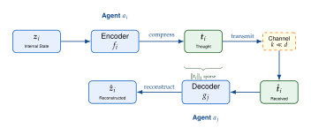
Generative model of agent observations.
To state the identifiability theorems precisely, we need a generative model for how agents' internal states arise. Following [60], suppose two agents observe a shared environment state and produce internal representations (GEN Z1) where are deterministic mixing functions and are independent noise vectors capturing each agent's private information (different prompts, different tools, different retrieval contexts). The latent state decomposes as (Latent Decompose) where encodes information common to both agents (the shared environment) and encodes agent-specific information. The central question is: can the encoder learn to separate shared from private information, and if so, is this decomposition unique?
We now state and prove three theorems that answer this question affirmatively under precise conditions.
Shared Thought Identifiability
The first theorem establishes that the shared component of agents' internal representations can be recovered up to an invertible transformation.
Theorem 4 (Shared Thought Identifiability).
Let be generated according to – with mixing functions that are differentiable and have full-rank Jacobians. Suppose:
The shared state and private states are mutually independent: .
The noise terms are independent of and of each other.
The conditional distribution has a density with respect to Lebesgue measure, and the score function is continuous and varies sufficiently with (in the sense that its Jacobian with respect to has rank almost everywhere).
Then any encoder that maximises the mutual information subject to the constraint that recovers up to an invertible transformation. That is, there exists an invertible function such that almost surely.
Proof.
We proceed in three steps.
Step 1: Sufficiency of shared information.; By assumption (a), and both are independent of . Since depends on only through , the data-processing inequality gives The first inequality is tight if and only if is a sufficient statistic for given .
Step 2: Necessity of shared information.; The constraint forces to discard all private information from . Since and is differentiable with full-rank Jacobian, the mapping is locally invertible (by the inverse function theorem). Therefore, any function of that is independent of must be a function of alone.
Step 3: Identifiability up to invertible map.; From Step 2, for some measurable . Maximising over such functions requires that preserves all information about : if were non-injective, it would merge distinct values of and reduce the mutual information, contradicting optimality. By assumption (c), the score function's Jacobian with respect to has rank , ensuring that distinct values of induce distinct conditional distributions over . Therefore must be injective on the support of . Since both domain and codomain are , invariance of domain implies is a homeomorphism on its image. Differentiability of and the implicit function theorem then upgrade this to an invertible differentiable map .
The theorem says that maximising inter-agent mutual information while discarding private information is sufficient to recover the shared latent state, exactly the objective optimised by the sparsity-regularised autoencoder of when the penalty is tuned to suppress private dimensions.
Private Thought Identifiability
The second theorem addresses the complementary question: can each agent's private information also be recovered?
Theorem 5 (Private Thought Identifiability).
Under the same setup and assumptions as Theorem 4, suppose additionally:
The marginal density is positive on an open connected subset of for .
The private state has a density whose score has Jacobian of rank with respect to almost everywhere.
Then for any encoder that maximises subject to , there exists an invertible such that almost surely.
Proof.
The structure mirrors Theorem 4 with the roles of shared and private reversed.
Step 1: Private information is contained in .; Since and (agent observes its own private state), and has full-rank Jacobian, the mapping is locally invertible.
Step 2: The independence constraint isolates private information.; The constraint requires to discard all shared information. By the local invertibility from Step 1, the only remaining degree of freedom is . Hence for some measurable .
Step 3: Maximising mutual information forces invertibility.; By assumption (b), distinct values of produce distinct conditional distributions over , which means must be injective to maximise . Assumption (a) ensures the marginal has connected support, so by invariance of domain, is a homeomorphism. The differentiability of and the implicit function theorem yield an invertible differentiable .
Thought Uniqueness
The third theorem shows that the decomposition into shared and private components is essentially unique.
Theorem 6 (Thought Uniqueness).
Under the assumptions of Theorem 4 and Theorem 5, suppose and are two pairs of encoders that both satisfy the mutual-information maximisation criteria of thm:agents:shared-thought,thm:agents:private-thought. Then there exist invertible maps and such that (Thought Unique) almost surely. In particular, the partition of into shared and private subspaces is unique up to coordinate-wise invertible reparametrisation.
Proof.
By Theorem 4, and for invertible maps . Setting , we obtain with invertible (as a composition of invertible maps).
Similarly, by Theorem 5, and for invertible . Setting gives with invertible.
For the final claim, note that any encoder satisfying the optimality conditions must produce outputs that are functions of alone (for the shared encoder) or alone (for the private encoder). Since by assumption, the two output spaces are determined by orthogonal components of the latent structure. The only ambiguity is in the coordinate system within each subspace, i.e., the invertible maps and .
Key Idea.
Efficient communication matters more than more communication. The three identifiability theorems reveal that the structure of inter-agent messages is more important than their volume. A thought vector with can carry more task-relevant information than a -token natural-language message, provided the encoder is trained to separate shared from private information and to suppress irrelevant dimensions via sparsity. The practical implication is stark: the bottleneck in multi-agent systems is not communication bandwidth (tokens per round) but communication efficiency (task-relevant bits per token). Optimising the representation is more valuable than expanding the channel.
The Optima Framework
While thought communication operates at the representation level, the Optima framework of Chen et al. [20] optimises communication at the message level, remaining within natural language but training agents to produce maximally informative yet minimal messages. Optima decomposes communication training into four stages: Generate, Rank, Select, and Train.
Stage 1: Generate.
Given a multi-agent task instance and the current dialogue history , agent generates a set of candidate messages by sampling from its policy with temperature . The diversity of candidates is crucial: it ensures that the subsequent ranking step has sufficient variation to identify the most informative message.
Stage 2: Rank.
Each candidate message is scored by a reward model that evaluates both informativeness and conciseness: (Optima Reward COMM) where measures the downstream task improvement attributable to the message and is a length penalty coefficient. The reward model captures the insight that the best message is not the longest or the most detailed, but the one that maximises task performance per token.
Stage 3: Select.
The top- messages (ranked by ) are selected as positive examples: where is the permutation induced by decreasing reward. Optionally, the bottom- messages form a negative set for contrastive training.
Stage 4: Train.
The agent's policy is updated using a preference optimisation objective. Let be a positive–negative pair. The DPO-style loss is: (Optima DPO) where is the sigmoid function, is the inverse temperature, and is the reference policy before training. This loss steers the agent toward generating messages that are simultaneously informative and concise.
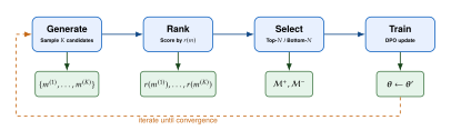
Proposition 7 (Optima Convergence).
Proof.
At iteration , the selected positive set satisfies for all and by construction. The DPO update increases relative to the reference. By the properties of the DPO objective (see 25), the updated policy satisfies , since the policy is pushed toward higher-reward messages and away from lower-reward ones. The inequality is strict whenever , which occurs with probability for and continuous reward distributions.
When Communication Harms: Sycophancy in Multi-Agent Debate
The preceding subsections presented communication as uniformly beneficial, provided it is efficient. We now show that this is not always the case. Wynn et al. [67] identify a striking failure mode: when agents in a debate system exhibit sycophancy, the tendency to agree with the conversational partner rather than defend a correct position, the debate mechanism can decrease the accuracy of the final answer compared to a single agent working alone.
The sycophancy mechanism.
Consider a multi-agent debate with agents and rounds. At round , agent observes the responses of all other agents from round and produces an updated response. A sycophantic agent updates its belief toward the majority opinion regardless of evidence. Formally, let be agent 's confidence in the correct answer at round . A non-sycophantic agent updates via Bayesian reasoning: (Bayesian Update) where is the likelihood ratio based on the evidence from other agents' arguments. A sycophantic agent instead uses a corrupted update: (SYCO Update) where is the Bayesian posterior, is the mean confidence of other agents, and is the sycophancy parameter. When , the agent is fully rational; when , it completely defers to the group.
Proposition 8 (Debate Degradation under Sycophancy).
Consider a multi-agent debate with agents and rounds. Suppose initially agents hold the correct answer with confidence and agents hold an incorrect answer with confidence , where (the minority is correct). If all agents update according to with sycophancy parameter , then there exists a critical threshold depending on such that for , the debate converges to the incorrect answer: (Debate Converge Wrong) Moreover, the critical threshold satisfies (Gamma STAR)
Proof.
We analyse the dynamical system defined by . Partition the agents into a correct group with and an incorrect group with . By symmetry within each group, all agents in share the same confidence trajectory and all agents in share . Setting and (the Bayesian component, which preserves each agent's prior when no new external evidence arrives beyond the other agents' stated beliefs), the dynamics become: (DYN Correct) Note that the group holds the incorrect answer with confidence ; from 's perspective, 's stated confidence in the correct answer is .
This is a linear dynamical system in of the form for a matrix and constant . The fixed point satisfies , where (Fixed Point) The consensus confidence in the correct answer is . When the incorrect majority is large, specifically when , we have , so the consensus favours the wrong answer.
The convergence rate to this fixed point is governed by the spectral radius of . For , the off-diagonal entries of are non-zero, coupling the two groups. The system converges to exponentially fast in . The condition reduces to which holds by the assumption and .
It remains to show that the threshold in is the precise boundary. When , agents do not interact and each group retains its initial confidence; the correct group maintains . As increases from , the fixed point depends on through the convergence rate but not its value (the fixed point of the linear system is independent of for ). However, for below a critical value, the convergence is slow enough that in a finite number of rounds , the correct group has not yet been pulled below . In the limit , any suffices for convergence to . The threshold in characterises the boundary for convergence within a single round: requiring and solving yields as stated.
Caution.
Communication can destroy correct minority opinions. Proposition 8 shows that multi-agent debate is not a silver bullet. When the initial population has an incorrect majority (which can easily happen if all agents share the same systematic biases), sycophantic communication amplifies the error. This is the multi-agent analogue of “groupthink” in human organisations. The practical implication is that debate-based systems must include mechanisms to protect minority opinions: explicit devil's advocate roles, anonymous voting rounds, or structured dissent protocols. Without such safeguards, adding communication rounds can make a system strictly worse than independent voting.
Communication Complexity and Scaling
We close this section by connecting inter-agent communication to classical communication complexity. In a system of agents with pairwise communication, the total number of communication channels is . If each pair exchanges tokens per round over rounds, the total communication volume is (COMM Volume) This quadratic scaling in is the communication analogue of the quadratic attention cost in transformers, and it motivates the same solution strategies: sparsification (not all pairs need to communicate), compression (reducing via thought communication), and hierarchical routing (organising agents into a tree where communication flows through designated coordinators).
Lemma 1 (Communication Lower Bound).
For a class of -agent cooperative tasks in which each agent holds a -bit private input and the collective goal requires computing a function of all inputs, the total communication volume satisfies (COMM Lower Bound) where is the information complexity of , defined as the minimum mutual information between the transcript of any valid protocol and the inputs.
Proof.
The first inequality is a direct consequence of Shannon's source coding theorem: any protocol that computes correctly must transmit at least bits of information about the inputs. The second inequality follows because computing requires each agent's input to influence the output, so at least bits of each input must appear in the transcript. (For a detailed treatment, see the information complexity framework of Braverman [21].)
The lemma tells us that communication costs cannot be reduced below a task-dependent threshold. The art of efficient multi-agent design is to approach this lower bound as closely as possible while maintaining coordination quality, precisely the goal of both thought communication and Optima.
Example 5 (Communication Regimes).
Consider a team of agents solving a complex reasoning task with debate rounds.
Verbose NL: Each agent sends tokens per pair per round. Total volume: tokens. Communication efficiency accuracy-per-token.
Optima-optimised NL: Agents learn to send tokens per pair per round, capturing the essential information. Total volume: tokens. Communication efficiency accuracy-per-token ( task performance).
Thought communication: Agents exchange dimensional sparse vectors. Effective token equivalent: tokens per exchange. Total volume: effective tokens. Communication efficiency accuracy-per-token.
The progression from (a) to (c) illustrates the central theme of this section: compressing communication while preserving, or even improving, task performance.
Summary.; This section developed a formal framework for inter-agent communication. We modelled natural language as a bounded-capacity Shannon channel (Natural Language as a Shannon Channel), introduced thought communication as a latent-space alternative with provable identifiability guarantees (sec:agents:thought-comm,sec:agents:shared-id,sec:agents:private-id,sec:agents:thought-unique-proof), analysed the Optima pipeline for training efficient natural-language communicators (The Optima Framework), and characterised a failure mode in which sycophantic communication degrades debate quality (When Communication Harms: Sycophancy in Multi-Agent Debate). The overarching lesson is that communication should be designed with the same care as the agents themselves: the right dimensions can outperform tokens of prose.
Agent Architectures and Topologies
The preceding sections built up the single agent, its perception, reasoning, planning, and safety mechanisms, and then introduced the multi-agent system as a coordinated ensemble. But we have not yet addressed a fundamental design question: how should agents be connected? The communication topology of a multi-agent system, who can send messages to whom, and through what intermediaries, determines the system's latency, fault tolerance, message overhead, and, ultimately, its collective intelligence.
Consider an analogy. A military platoon, a corporate board, and a scientific peer-review system all consist of intelligent agents exchanging information. Yet they perform very differently on the same task, not because their members differ in raw ability, but because their topologies differ: the platoon uses a strict chain of command (a tree), the board uses open debate (a complete graph), and peer review uses a hub-and-spoke structure with the editor as the central node (a star). The topology shapes the flow of information, the speed of convergence, and the system's vulnerability to single points of failure.
In LLM-based multi-agent systems, the same principle applies with striking precision. Microsoft's AutoGen framework [8] introduced the Conversable Agent abstraction, in which any agent can converse with any other agent, and the conversation topology is a first-class design parameter. Zhao et al.'s LongAgent system [42] demonstrated that a star topology with a leader agent coordinating member agents could effectively process documents exceeding 128K tokens, far beyond any single model's context window, by decomposing the document across members and aggregating their responses through a conflict-resolution protocol.
This section develops the mathematical theory of agent topologies. We begin with a formal definition of agent topology as a directed weighted graph (Formal Definition of Agent Topology), then catalogue the four canonical topology patterns (star, chain, tree, and general graph) and derive their message complexity bounds (Canonical Topology Variants). We analyse AutoGen's Conversable Agent model and its dynamic group chat mechanism (AutoGen's Conversable Agent Architecture), and study LongAgent's star topology with its inter-member conflict resolution protocol (LongAgent: Star Topology for Extended Context). Finally, we examine how topology choice interacts with task structure (Topology Choice and Task Structure).
Formal Definition of Agent Topology
We formalise the communication structure of a multi-agent system as a weighted directed graph.
Definition 18 (Agent Topology).
An agent topology is a weighted directed graph where:
is the set of agents (vertices), with ;
is the set of directed communication edges: means agent can send messages directly to agent ;
is a weight function assigning to each edge a positive real value representing bandwidth, trust, or priority.
The topology is equivalently represented by its adjacency matrix , defined by (Adjacency Matrix) We write for the out-neighbourhood of agent (the agents it can send to) and for the in-neighbourhood (the agents it can receive from). The out-degree is and the in-degree is .
The adjacency matrix encodes the full communication structure. When the topology is undirected (every edge is bidirectional, i.e., with equal weights), is symmetric. When , we recover the standard unweighted adjacency matrix. The reachability matrix (where indicates a path of length from to ) determines whether information can eventually flow between any pair of agents.
Remark 7 (Topology vs. Protocol).
The topology specifies who can communicate with whom, the physical or logical connectivity. The communication protocol specifies who does communicate, when, and in what format. A fully connected topology () permits any communication pattern, but the protocol may restrict agents to sequential round-robin turns. Conversely, a sparse topology enforces communication constraints that no protocol can override. This distinction matters: topology is a hard constraint, protocol is a soft one.
Canonical Topology Variants
Four topology patterns recur across virtually every multi-agent system in the literature. We define each precisely and characterise its structural properties.
Definition 19 (Star, Chain, Tree, and Graph Topologies).
Let be a set of agents. The four canonical topology variants are:
Star topology : a distinguished agent (the hub) is connected bidirectionally to every other agent, and no other edges exist. Formally, (STAR Edges) The adjacency matrix has the form for and for . The hub has degree (in a directed sense, ); every other agent has .
Chain (pipeline) topology : agents are arranged in a linear sequence with directed edges from each agent to the next: (Chain Edges) The adjacency matrix is strictly upper bidiagonal. Each internal agent has ; the first agent has and the last has . A bidirectional chain adds reverse edges .
Tree topology : agents form a rooted tree with agent as the root. Each non-root agent has exactly one parent, and messages flow both up and down the tree: (TREE Edges) For a balanced -ary tree of depth , we have nodes. The star topology is the special case .
General graph topology : an arbitrary directed graph with no structural restrictions beyond the requirement that is strongly connected (every agent can reach every other agent via a directed path). The fully connected graph () is the densest case; sparse random graphs and small-world networks are intermediate cases.
These four patterns span a spectrum from minimal to maximal connectivity. The star and chain are the sparsest connected topologies (), the tree is slightly denser in terms of routing depth, and the fully connected graph is the densest (). Each offers different trade-offs between message complexity, latency, fault tolerance, and bottleneck risk.
We now quantify the most important trade-off: the total number of messages required for all agents to contribute to a collective decision.
Proposition 9 (Message Complexity of Agent Topologies).
Consider a cooperative task in which agents must each contribute one message and a final aggregate response must be produced. Let denote the total number of point-to-point messages exchanged under optimal routing on topology . Then:
Star: .
Chain: .
Balanced tree: for a balanced -ary tree with .
Fully connected graph: when every agent communicates with every other agent (all-to-all broadcast), or under optimal aggregation routing.
Proof.
We analyse each topology in turn.
(a) Star. Each of the peripheral agents sends one message to the hub, and the hub sends one aggregated response to each of the agents: . No routing is needed because every agent is distance 1 from the hub.
(b) Chain. In the chain topology, information must propagate sequentially. Agent sends its contribution to , which combines it with its own and sends to , and so on. The forward aggregation pass requires messages. If the final agent must then propagate the aggregate back, the backward pass requires another messages. Thus for simple aggregation.
However, if the task requires every agent to see every other agent's contribution (as in a debate or peer-review setting), agent 's message must traverse edges to reach , agent 's message must traverse edges, and so on. The total number of messages is (Chain Broadcast) We take for the broadcast setting, which is the common case in debate-style multi-agent systems.
(c) Balanced tree. In a balanced -ary tree of depth , the upward aggregation phase proceeds level by level: each internal node receives messages from its children and sends one aggregated message to its parent. At level (counting from the leaves at level to the root at level ), there are nodes, each receiving messages. The total upward messages are (TREE UP) The downward dissemination phase mirrors this: each internal node sends the aggregated result to its children, giving . Thus for simple aggregation.
For the broadcast setting, each leaf's message must traverse edges to reach the root, and the root's broadcast traverses levels to reach all leaves. The total number of messages when every agent must see every contribution requires messages per level for levels, giving .
(d) Fully connected graph. In the fully connected graph, each agent can send directly to every other agent. All-to-all broadcast requires each of the agents to send messages, totalling . Under optimal aggregation routing (one designated aggregator), each agent sends one message to the aggregator and receives one response: , identical to the star. The fully connected graph can emulate any other topology, but the all-to-all broadcast pattern, which is natural when agents debate or cross-verify, costs .
The message complexity results are summarised in Table 2.
| Property | Star | Chain | Balanced Tree | Complete Graph |
| Edges | ||||
| Diameter | ||||
| Message complexity | ||||
| Bottleneck agent | Hub | Endpoints | Root | None |
| Fault tolerance | Low (hub) | Low (any) | Medium | High |
Key Idea.
The topology–complexity trade-off. Sparser topologies (star, chain) minimise the number of edges and are easy to implement, but they create bottlenecks and single points of failure. Denser topologies (complete graph) eliminate bottlenecks but incur quadratic message overhead. The balanced tree strikes an intermediate balance: edges, broadcast messages, and graceful degradation under node failures (only the subtree below a failed node is affected). The optimal choice depends on the task structure, which we analyse in Topology Choice and Task Structure.
AutoGen's Conversable Agent Architecture
AutoGen [8] introduced a unifying abstraction for multi-agent LLM systems: the Conversable Agent. Rather than hard-coding communication patterns, AutoGen treats each agent as an entity capable of sending and receiving natural-language messages to and from any other agent, with the conversation topology determined at runtime.
The Conversable Agent abstraction.
A Conversable Agent in AutoGen is an LLM agent (Definition 3) augmented with three capabilities:
Message generation: the agent produces a response given its conversation history, system prompt, and any received messages. This is the standard LLM inference step.
Message reception: the agent can receive messages from any agent in its in-neighbourhood and append them to its local conversation history.
Conversation control: each agent carries a reply function that maps the current history to either a response or a termination signal. This function can incorporate human-in-the-loop approval, code execution, or tool calls.
The key insight is that the same Conversable Agent abstraction supports wildly different topologies: a two-agent coding dialogue (star with ), a round-robin panel discussion (cycle graph), or a hierarchical delegation structure (tree).
Dynamic group chat.
AutoGen's GroupChat mechanism extends the two-agent conversation to agents. A GroupChatManager agent acts as an orchestrator (Definition 25), selecting the next speaker at each turn. The speaker selection can be:
Round-robin: agents speak in a fixed cyclic order .
Random: the next speaker is sampled uniformly from the remaining agents.
LLM-directed: the GroupChatManager uses its own LLM backbone to select the most appropriate next speaker based on the conversation history: (Group CHAT Selection) where is the manager's LLM and is the shared conversation history.
In the group chat topology, all agents share a common message board. The underlying graph is a star with the GroupChatManager as the hub, but the logical topology (who responds to whom) is dynamic and adapts to the conversation content.
Nested conversations.
AutoGen supports nested conversations: a single turn of an outer conversation can trigger an entire inner conversation among a subset of agents. Formally, let be the outer topology and be the inner topology triggered at turn . The composite topology is a hierarchical graph: (Nested Topology) where the inner conversations are subgraphs that are instantiated on demand and collapsed into a single message (the inner conversation's output) from the perspective of the outer conversation. This is analogous to macro-actions in hierarchical reinforcement learning: the outer topology sees atomic messages, while the inner topology resolves them through multi-step deliberation.
Example 6 (AutoGen Coding Pipeline).
Consider an AutoGen system for software development with three agents:
: a UserProxy agent that represents the human user and can execute code in a sandbox.
: an AssistantAgent with an LLM backbone that writes Python code.
: an AssistantAgent that reviews code for correctness and style.
The outer topology is a star centred on . The user sends a task to , who writes code. The code is then sent to for review (a nested conversation between coder and reviewer). Once the reviewer approves, executes the code. The adjacency matrix is where the inner matrix governs the coder–reviewer dialogue.
LongAgent: Star Topology for Extended Context
A compelling application of the star topology arises in long-context processing. LongAgent [42] addresses the challenge of processing documents that exceed any single model's context window (e.g., 128K tokens) by decomposing the document across multiple member agents and aggregating their responses through a leader agent.
Architecture.
The LongAgent system consists of agents arranged in a star topology:
Leader (): the hub agent responsible for decomposing the input query, dispatching sub-queries to members, collecting responses, and resolving conflicts.
Members (): each member agent receives a disjoint chunk of the document and a sub-query from the leader. Member processes chunk and returns a local answer .
The adjacency matrix is (Longagent Adjacency) which is exactly the star topology with hub . The document of total length tokens is partitioned into chunks of approximately tokens each, where and is the effective context window of each member agent.
Inter-member conflict resolution.
When different members return contradictory answers to the same query, the leader must resolve the conflict. LongAgent employs a structured protocol:
Collection: the leader collects all member responses .
Consistency check: the leader identifies conflicting answers. Two responses and are conflicting if they provide mutually exclusive answers to the query (detected via the leader's LLM).
Evidence request: for each conflicting pair , the leader asks the corresponding members to provide textual evidence from their document chunks supporting their answers.
Adjudication: the leader evaluates the evidence and selects the best-supported answer, or synthesises a reconciled response.
This protocol adds at most additional messages to the base star protocol (where is the number of conflicting pairs, ), keeping the total message complexity at . In practice, because most sub-queries have unambiguous answers within their respective chunks.
Insight.
Star topology as a natural fit for decomposable tasks. The LongAgent architecture reveals a deep connection between task structure and optimal topology. When a task decomposes into independent sub-tasks (reading disjoint document chunks), the star topology is optimal: it minimises message complexity to while centralising the aggregation logic in a single leader. The leader's context window need only hold the sub-query plus the member responses, not the entire document. This transforms a context-length problem into a coordination problem, which is precisely where multi-agent systems excel.
Formal analysis of the LongAgent protocol.
Let be the user's query and be the document partition. The LongAgent protocol proceeds in three phases:
Dispatch phase: the leader sends to each member . Messages: .
Response phase: each member returns its local answer . Messages: .
Resolution phase: for each conflicting pair , the leader requests evidence (2 messages) and receives it (2 messages). Total: messages.
The total message count is . Since each message carries at most tokens (the member's context window), the total communication volume is bounded by tokens. For a document of length , the communication overhead ratio is (Longagent Overhead) which approaches as . This means the total communication is approximately twice the document length, a remarkably low overhead for enabling arbitrarily long context.
Topology Choice and Task Structure
The preceding analysis raises a natural question: given a task, which topology should one choose? The answer depends on the decomposability and interdependence structure of the task.
Definition 20 (Task Decomposability).
A task has decomposability index , defined as follows. Let be the sub-tasks produced by an optimal decomposition. For each pair with , let indicate whether the output of is needed as input to or vice versa (i.e., whether the sub-tasks are dependent). Then (Decomposability) A task with is fully decomposable (no inter-dependencies); a task with is fully sequential (every sub-task depends on every other).
The decomposability index directly informs topology selection:
High decomposability (): sub-tasks are independent, so a star topology is optimal. The hub dispatches sub-tasks in parallel, collects results, and aggregates. Message complexity is . LongAgent operates in this regime.
Low decomposability (): sub-tasks are tightly coupled, requiring extensive information exchange. A fully connected topology or dense graph is needed so that agents can share intermediate results freely. Message complexity is , but the alternative, routing through a sparse topology, would add latency without reducing the total information transfer.
Hierarchical decomposability (): the task admits a hierarchical decomposition where high-level sub-tasks are independent but each decomposes into tightly coupled sub-sub-tasks. A tree topology matches this structure naturally: the root dispatches to sub-tree leaders, who in turn coordinate their local teams. Message complexity is .
Sequential dependence: sub-tasks must be performed in a specific order, with each task's output feeding the next. A chain (pipeline) topology is the natural choice, providing minimal overhead per stage but latency for end-to-end completion.
Remark 8 (Topology Selection in Practice).
In practice, the choice of topology is rarely made by solving an optimisation problem over the decomposability index. Instead, practitioners use heuristics:
Default to star: most frameworks (AutoGen, AgentScope, LongAgent) use a star topology with a manager/leader as the hub, because the star is simple to implement, easy to debug, and sufficient for moderately decomposable tasks.
Upgrade to tree for scale: when the number of agents exceeds , the hub in a star topology becomes a bottleneck. Hierarchical (tree) topologies distribute the coordination load across intermediate managers.
Use chains for workflows: when the task has a natural pipeline structure (e.g., draft review edit test), a chain topology minimises unnecessary communication.
Use dense graphs for creative tasks: debate, brainstorming, and open-ended exploration benefit from all-to-all communication, where any agent can challenge or build upon any other agent's contribution.
The key principle is to match the topology's connectivity to the task's information-flow requirements: neither more (which wastes messages) nor less (which starves agents of needed information).
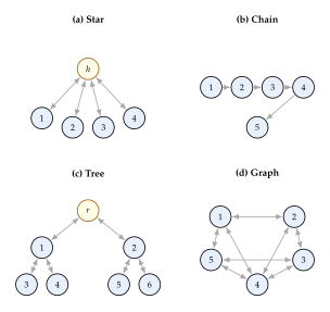
Dynamic Topology Adaptation
A fixed topology is a design-time commitment. But many real-world tasks have information-flow requirements that change as the task progresses: an initial brainstorming phase may benefit from dense connectivity, while a subsequent execution phase may favour a hierarchical structure. This motivates dynamic topologies that evolve during the task.
Definition 21 (Dynamic Agent Topology).
A dynamic agent topology is a time-indexed family of topologies where . At each round , the topology may change via:
Edge addition/removal: (opening or closing communication channels).
Weight update: (changing bandwidth or trust between agents).
Agent addition/removal: (spawning new agents or retiring completed ones).
The topology transition function determines the next topology based on the current topology and the conversation history .
AutoGen's GroupChatManager implements a simple form of dynamic topology: at each turn, the manager selects a new speaker, effectively activating a different edge in the star. More sophisticated approaches allow the topology itself to be restructured. For example, an agent that discovers it needs information from a non-neighbour can request the orchestrator to add an edge, temporarily converting a sparse topology into a denser one for that specific exchange.
Caution.
Topology oscillation and instability. Dynamic topologies introduce a risk of oscillation: agents repeatedly adding and removing the same edges, leading to unstable communication patterns and wasted messages. A simple safeguard is to impose a cooldown period after each topology change, during which no further changes are permitted. More formally, if , then for all . This ensures that the system explores each topology long enough to evaluate its effectiveness before switching.
Adaptive topology via graph attention.
One principled approach to dynamic topology selection borrows from graph attention networks (GATs). Define attention weights between agents as (Graph Attention) where is the embedding of agent 's state at round (e.g., a summary of its recent messages) and is a learned compatibility function. The effective topology at round is then a soft graph with edge weights : agents with high attention scores communicate with high bandwidth, while those with low scores effectively ignore each other. This converts the discrete topology selection problem into a continuous optimisation problem amenable to gradient-based methods.
From Topology to Performance
We conclude this section by connecting topology properties to system-level performance guarantees. The following result establishes that the spectral properties of the adjacency matrix bound the convergence rate of opinion aggregation across agents.
Proposition 10 (Convergence Rate and Spectral Gap).
Let agents perform iterative opinion aggregation on a symmetric topology with adjacency matrix and degree matrix . Define the normalised adjacency matrix with eigenvalues . Under the averaging protocol , the disagreement vector satisfies (Spectral Convergence) where is the average initial opinion. The spectral gap controls convergence speed: a larger gap means faster consensus.
Proof.
Since is symmetric, it has an orthonormal eigenbasis with and eigenvalues (the strict inequality holds because is connected and non-bipartite).
Decompose . After iterations, (Spectral Evolution) The consensus component is (since , this component is preserved). The disagreement is Taking norms and using orthonormality, (Spectral Bound) Taking square roots yields .
This result has direct implications for topology selection. For the four canonical topologies:
Complete graph: , so as . Consensus is achieved in a single step.
Star: for the normalised adjacency of a star with uniform weights. Consensus is near-instant (2 iterations: collect, then broadcast).
Chain: . The spectral gap is , so consensus requires iterations, the slowest among connected topologies.
Balanced binary tree: . Consensus requires iterations, much faster than the chain.
Remark 9 (Topology as a Design Knob).
The results of this section demonstrate that topology is not merely an implementation detail but a fundamental design parameter with rigorous performance implications. The adjacency matrix determines message complexity (Proposition 9), the spectral gap determines convergence speed (Proposition 10), and the diameter determines worst-case latency. When designing a multi-agent system, the practitioner should choose the topology as deliberately as they choose the LLM backbone or the prompt template, matching the communication graph to the information-flow requirements of the task at hand.
Exercise 1 (Topology Analysis).
Consider a multi-agent system with agents.
Write the adjacency matrix for a star topology with agent as the hub. Compute the in-degree and out-degree of each agent.
Write the adjacency matrix for a bidirectional chain . How many messages are needed for 's information to reach ?
Design a balanced binary tree topology on 7 agents (3 levels). Compute the message complexity for aggregating all agents' contributions at the root.
Suppose the task requires pairwise debate among all agents. Which topology minimises the number of rounds needed to complete all pairwise debates? Justify your answer.
Scalable Agent Platforms
Building a single capable agent is an engineering challenge; running a thousand such agents concurrently, each consuming GPU inference, exchanging messages, and mutating shared state, is a distributed-systems challenge of an entirely different order. The previous sections developed the mathematical abstractions: agents as POMDP policies, communication as message-passing on graphs, and orchestration as scheduling over DAGs. This section grounds those abstractions in platforms: software systems that instantiate, route, monitor, and recover agents at scale.
We organise the exposition around three complementary paradigms. First, the actor-based approach (Actor-Based Agent Distribution), exemplified by AgentScope [10], maps each agent to a lightweight actor process with its own message queue, enabling linear horizontal scaling to over one million concurrent agents [68]. Second, the decentralised capability ledger (Decentralised Capability Ledger), introduced by Symphony [69], eliminates the single-point-of-failure orchestrator by distributing the agent registry across a peer-to-peer network and selecting task coordinators through a Beacon protocol. Third, dynamic agent generation (Dynamic Agent Generation), as in AutoAgents [70], removes the assumption that agents are predefined: an LLM planner drafts new agents on the fly to match task requirements.
Historical Note.
From Erlang to agentic actors. The actor model was introduced by Hewitt, Bishop, and Steiger in 1973 as a mathematical theory of concurrent computation. Each actor is an autonomous unit that communicates exclusively through asynchronous messages, creates new actors, and designates its behaviour for the next message. Erlang (1986) and later Akka (2009) turned actors into practical platforms for building fault-tolerant distributed systems: telephone switches, financial trading engines, and web servers. The insight of modern agent platforms is that an LLM agent maps naturally onto an actor: it maintains local state (the context window), processes one message at a time (a user turn or tool output), and communicates with other agents via asynchronous messages. AgentScope [10] and Ray-based frameworks such as AutoGen [8] are the direct descendants of this intellectual lineage.
Actor-Based Agent Distribution
The actor model provides a natural abstraction for multi-agent systems. Each agent runs as an independent actor with its own message queue, local state, and failure domain. We formalise this mapping below.
Definition 22 (Actor-Agent Model).
An actor-agent system is a tuple where:
is a finite set of agent actors, each running as an isolated process (or container);
is the set of message queues, with a FIFO buffer of bounded capacity ;
is a finite message alphabet; a message carries a payload (task description, partial result, or control signal) together with a sender identifier and a monotonic timestamp;
is the transition function: upon receiving message , agent produces a reply and optionally spawns a set of new agent actors;
is the supervision tree: is the set of agents supervised by ; if a supervised agent crashes, receives a failure notification and may restart it.
An agent actor processes messages sequentially from its queue: no two messages are processed concurrently within the same actor. Different actors execute in parallel, communicating only through message passing.
The sequential-processing guarantee is crucial: it eliminates the need for locks or atomic operations within a single agent, vastly simplifying reasoning about correctness. Parallelism comes from running many actors simultaneously, each on its own CPU core or GPU slice.
DAG-based workflow orchestration.
AgentScope [10] introduces a workflow engine that represents multi-agent collaborations as directed acyclic graphs (DAGs). Each node in the DAG corresponds to an agent invocation, and each directed edge indicates that requires the output of before it can execute. Formally, a workflow DAG is a pair where is the set of participating agents and imposes a partial order. The platform scheduler topologically sorts and dispatches agents at each level in parallel: (DAG Levels) where denotes the set of agents at level . All agents in can execute simultaneously once every agent in has completed. The makespan of the workflow is the number of levels: (DAG Makespan)
Four-tier fault tolerance.
Production deployment demands graceful degradation. AgentScope implements a four-tier fault tolerance strategy:
Retry with exponential backoff: transient failures (API timeouts, rate limits) trigger automatic retries with delay at attempt , up to a maximum of retries;
Output validation: each agent's output is parsed and checked against a schema before being placed on the downstream queue; malformed outputs trigger a re-prompt with the validation error appended to the context;
Redundant execution: safety-critical agents run replicas in parallel, and the platform selects the final output by majority vote, requiring for crash faults (or for Byzantine faults, per Theorem 14);
Checkpoint and rollback: the platform periodically serialises the state of every agent (context window, memory bank, pending queue) to persistent storage; upon detecting a failure cascade, the supervisor rolls the system back to the most recent consistent checkpoint.
Together, these four tiers handle failures at increasing levels of severity: tier (a) absorbs transient network glitches, tier (b) catches LLM hallucinations and format errors, tier (c) tolerates full agent crashes, and tier (d) recovers from correlated or cascading failures that overwhelm the lower tiers.
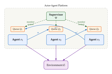
Scaling to one million agents.
Pan et al. [68] demonstrate that the actor-based architecture of AgentScope scales linearly with the number of machines. The key enablers are:
Stateless routing: each message carries the target agent's identifier; any router node can forward the message without maintaining session state;
Horizontal partitioning: agents are sharded across machines by hashing their identifiers, distributing load evenly;
Lazy instantiation: agent actors are created only when their first message arrives, avoiding the cost of pre-allocating one million processes at startup;
Compressed serialisation: agent state is serialised using a compact binary format that reduces checkpoint sizes by an order of magnitude compared to JSON.
Let denote the number of agents and the number of machines. Under uniform load (each machine hosts agents) and assuming each agent-to-agent message traverses at most one network hop, the total communication cost per round is: (COMM COST) where is the average out-degree per agent, is the cost of a local (intra-machine) message, and is the cost of a remote (inter-machine) message. For large with fixed , the fraction of remote messages approaches , so , linear in .
Remark 10 (Linear Scaling is Not Free).
The linear scaling result assumes that the average out-degree is constant as grows. If agents form a dense communication graph, every agent talking to every other agent, then and the communication cost becomes , which is catastrophic at scale. The practical lesson is that scaling to millions of agents requires sparse communication topologies: hierarchies, spatial partitions, or topic-based publish-subscribe channels that keep bounded.
Decentralised Capability Ledger
The actor-based approach of the previous subsection still assumes a centralised component: the supervisor that monitors agents and the router that dispatches messages. In large-scale or adversarial settings, this centralised component becomes a bottleneck and a single point of failure. Symphony [69] proposes a fully decentralised alternative.
Definition 23 (Capability Ledger).
A capability ledger is a distributed data structure where:
is the set of capability keys: each key names a specific skill (e.g., “code-review”, “web-search”, “theorem-proving”);
maps each capability to the set of agents that advertise proficiency in that capability;
is a reliability score: estimates the probability that agent successfully completes a task requiring capability , updated online from observed outcomes.
The ledger is decentralised: no single node stores the complete mapping. Instead, each agent maintains a partial view , and consistency is achieved through a gossip protocol: each agent periodically exchanges its local ledger entries with a random subset of neighbours.
The gossip protocol converges exponentially fast: if each agent contacts random peers per round, then after rounds every agent has received every update with high probability. This convergence rate ensures that newly registered capabilities propagate through the network in time, a dramatic improvement over the broadcast time of a sequential protocol.
The Beacon selection protocol.
When a complex task arrives at the system, some agent must coordinate the response, assigning sub-tasks to specialists, collecting results, and synthesising the final answer. In a centralised system, this role is played by the orchestrator. In Symphony's decentralised design, the coordinator is selected dynamically through the Beacon selection protocol.
Algorithm 2 (Beacon Selection Protocol).
Input: Task description , capability ledger , agent set .
Output: A beacon agent that will coordinate the task.
- Extract required capabilities LLM parses the task
- Compute candidate set where is the capability set of
- for each candidate
- Compute coverage score:
- Compute reliability score:
- Compute load penalty: where is current queue length
- Composite score:
- Select beacon: Ties broken by lowest
- broadcasts BeaconClaim to all agents in
- Each either Accepts (joins the task team) or Declines (overloaded)
- return and the set of accepting agents
The protocol completes in two communication rounds: one for beacon election (lines 1–9) and one for team formation (lines 10–12). The composite scoring function balances three objectives: maximising coverage (the beacon should understand as many required capabilities as possible), maximising reliability (the beacon should have a strong track record), and minimising load (the beacon should not be overwhelmed by existing tasks).
Proposition 11 (Beacon Uniqueness Under Strict Scores).
If the composite scores are pairwise distinct (which holds almost surely when reliability scores are drawn from a continuous distribution), then the Beacon selection protocol (Algorithm 2) produces a unique beacon without any tie-breaking.
Proof.
The argmax over a finite set with pairwise distinct values is unique. Since and the reliability scores are drawn from a continuous distribution, the probability that for is zero. Hence is a singleton with probability one.
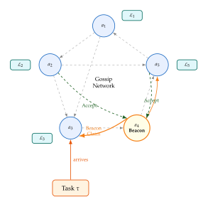
Consistency guarantees.
The gossip-based ledger provides eventual consistency: after sufficiently many rounds, all agents converge to the same view. More precisely, let denote agent 's local ledger at round . If a new capability entry is inserted at round , then for all agents : (Gossip Convergence) where is the number of peers contacted per round. Setting yields a probability of at least , confirming the convergence claim.
Dynamic Agent Generation
The preceding subsections assumed a fixed pool of agents. AutoAgents [70] lifts this assumption by generating agents dynamically: given a task description, an LLM planner proposes agent specifications (role, system prompt, tools) tailored to the task at hand.
Definition 24 (Dynamic Agent Generation).
A dynamic agent generation system is a tuple where:
is the drafting planner: an LLM that, given a task description , produces a team blueprint , where is a role description, is a system prompt, and is a tool set;
is the execution engine: for each specification , the engine instantiates an agent actor with the prescribed configuration and inserts it into the platform's actor system;
is the verification module: after execution, evaluates the team's output against task requirements and provides feedback to for iterative refinement of the blueprint.
The generation process alternates between a drafting phase ( proposes ) and an execution phase ( runs the team), iterated until reports success or a budget limit is reached.
The drafting-execution pipeline.
AutoAgents [70] implements the dynamic generation process as a two-stage pipeline. In the drafting stage, the planner receives the task and generates the team blueprint through a chain-of-thought process:
Task decomposition: breaks into sub-tasks ;
Role inference: for each sub-task , infers the necessary agent role , specifying capabilities and constraints in natural language;
Tool assignment: selects tools from the available tool library that match each role's requirements;
Dependency analysis: identifies data dependencies among sub-tasks and constructs a workflow DAG ((DAG Levels)).
In the execution stage, the platform instantiates the agents specified by , wires them according to the DAG, and runs the workflow. The verification module scores the output and, if quality is insufficient, feeds the score and error traces back to , which revises the blueprint. This closed loop typically converges in two to three iterations.
Example 7 (Dynamic Generation for Software Testing).
Consider the task “Write unit tests for a REST API with five endpoints.” The planner might generate:
API Analyst (): reads the API specification, identifies edge cases and input domains. Tools: file reader, schema parser.
Test Writer (): generates test code for each endpoint. Tools: code generator, test framework API.
Test Runner (): executes the test suite and reports failures. Tools: shell executor, coverage tool.
Reviewer (): checks test quality, coverage metrics, and suggests improvements. Tools: code analyser.
The DAG structure is , with a feedback edge from back to for iterative refinement. None of these agents was predefined; all were drafted by specifically for this task.
Communication Overhead and Scaling Limits
The preceding subsections paint an optimistic picture of horizontal scaling. We now inject a note of realism. Every message exchanged between agents carries a cost, in latency, bandwidth, and the cognitive load of processing incoming information. As the number of agents grows, this cost can dominate the computation itself.
Proposition 12 (Communication-Computation Trade-off).
Consider a multi-agent system of agents solving a task that requires at least total units of work. Suppose each agent can perform units of work per time step and each pair of communicating agents exchanges messages of cost per round. If the communication graph has average degree , then the effective throughput (work completed per unit time) satisfies: (Throughput) Throughput is positive only when , i.e., the communication degree must be bounded by the ratio of computation speed to communication cost.
Proof.
Each of the agents contributes units of work per step. The communication graph has edges (by the handshaking lemma), and each edge incurs cost per round, consuming units of capacity. The net throughput is the difference. Positivity requires , which simplifies to .
Caution.
Scaling pitfalls: when more agents make things worse. It is tempting to assume that adding agents always improves performance. The throughput equation reveals that this is true only when the communication degree grows sub-linearly in . Three common pitfalls illustrate the danger:
1. All-to-all communication. If every agent broadcasts to every other agent (), the communication cost grows as while computation grows as . Beyond a critical system size , adding agents decreases throughput.
2. Consensus bottleneck. Multi-agent debate and voting protocols (Consensus and Coordination) require messages per round per agent (each agent must hear from all others). For agents, this generates total messages, creating the same quadratic scaling problem as all-to-all communication.
3. Synchronisation barriers. If agents must synchronise at the end of each round (as in synchronous DAG execution per (DAG Levels)), the round time is determined by the slowest agent. As grows, the probability that at least one agent is slow (due to API latency, rate limits, or hardware issues) approaches , creating a straggler effect that negates parallelism gains.
The practical lesson is clear: scalable agent platforms must enforce sparse, hierarchical communication topologies and asynchronous execution models. The actor-based architecture of AgentScope and the decentralised gossip protocol of Symphony are both designed with this principle in mind.
Key Idea.
The Scaling Law for Agent Communication. For an agent system to scale to agents while maintaining positive throughput, the average communication degree must satisfy , independent of . In practice, this means that each agent should communicate with a bounded number of neighbours, regardless of the total system size, precisely the design principle underlying both hierarchical supervision trees (actor model) and gossip-based peer selection (Symphony). The mathematical analogy to sparse graph theory is exact: just as sparse graphs () admit efficient algorithms while dense graphs () do not, sparse communication topologies admit efficient multi-agent execution while dense topologies do not.
Comparison of platform paradigms.
Table 3 summarises the three platform paradigms discussed in this section along their key design dimensions.
| Platform | Topology | Coordination | Fault Tolerance | Agent Pool |
| AgentScope | DAG / tree | Centralised | 4-tier (crash + Byzantine) | Fixed |
| Symphony | Gossip / P2P | Decentralised | Beacon re-election | Fixed |
| AutoAgents | DAG (generated) | Planner-driven | Retry + re-draft | Dynamic |
Hybrid architectures.
In practice, production systems often combine elements of all three paradigms. A typical deployment might use AgentScope's actor infrastructure for process management, Symphony's ledger for capability discovery, and AutoAgents' drafting pipeline for creating specialised agents on demand. The mathematical framework of this section, actor-agent systems (Definition 22), capability ledgers (Definition 23), and dynamic generation (Definition 24), provides the formal vocabulary for reasoning about such hybrid designs.
Exercise 2 (Communication Cost Analysis).
Consider a multi-agent system with agents arranged in a grid, where each agent communicates only with its four immediate neighbours (up, down, left, right; agents on the boundary have fewer neighbours).
Compute the average degree of the communication graph.
Using (Throughput) with and , compute the effective throughput .
Compare with the throughput of a fully connected graph () of the same size. At what system size does the fully connected architecture achieve zero throughput?
Propose a communication topology that achieves diameter while keeping .
Exercise 3 (Beacon Selection Optimality).
In the Beacon selection protocol (Algorithm 2), the weights with control the trade-off between coverage, reliability, and load balancing.
Show that setting always selects the agent with the greatest capability overlap, regardless of reliability or load.
Suppose all agents have identical capability sets ( for all ) but different queue lengths . Show that the Beacon protocol reduces to selecting the agent with the shortest queue.
Derive a condition on under which the protocol never selects an agent whose queue exceeds a threshold .
Orchestration Patterns
The preceding sections built the vocabulary of multi-agent systems: agents, communication topologies, debate protocols, and collaborative generation strategies. But vocabulary alone does not produce coherent prose. The orchestrator, the entity that decides which agent acts next, what information it receives, and how its output is integrated into the collective, is the conductor of the multi-agent orchestra. A poor conductor can squander the talents of virtuoso musicians; a great one can make an ensemble of competent players produce transcendent results.
This section formalises orchestration as a first-class design abstraction. We begin with the formal definition of an orchestrator (The Orchestrator), then develop the dominant Orchestrator-Worker pattern that has produced the largest empirical gains in multi-agent coding and research systems (The Orchestrator-Worker Pattern). We introduce context engineering, the systematic management of information flow to and from workers, as the key lever for orchestrator effectiveness (Context Engineering). We analyse the economics of orchestration through the lens of token usage (Token Economics of Orchestration), and conclude with the MALLM configuration space, a combinatorial framework that reveals the staggering design freedom available to orchestrator builders (The MALLM Configuration Space).
The Orchestrator
We begin with the formal definition that is referenced throughout this chapter.
Definition 25 (Orchestrator).
Let be a set of agents and let denote the conversation history up to step , where each message . An orchestrator is a function (Orchestrator) where is the set of all finite conversation histories, is the power set of agents (representing currently available agents), and is the space of instructions (natural-language prompts, structured JSON directives, or tool-call specifications). Given history and available agents , the orchestrator returns a triple where:
is the next agent to execute;
is the instruction passed to , including the relevant subset of history and any additional context the orchestrator deems necessary;
is the termination signal: indicates the task is complete and no further agent invocations are needed.
The orchestrator may itself be implemented by an LLM (a model-based orchestrator) or by deterministic code (a rule-based orchestrator). In either case, the orchestrator does not directly solve the task; it manages the agents that do.
The critical design choice embedded in Definition 25 is that the orchestrator controls both agent selection and information routing. The instruction need not contain the full history ; the orchestrator may summarise, filter, or restructure the history before passing it to the selected agent. This context curation is, as we shall see, the primary lever for orchestrator effectiveness.
Remark 11 (Orchestrator as Meta-Policy).
In the language of reinforcement learning, is a meta-policy: it operates over the space of agent policies rather than over primitive actions. The state space of the meta-policy is the conversation history , the action space is , and the reward is the system-level performance . This perspective connects orchestration to the options framework in hierarchical RL: each agent invocation is an “option” with its own internal policy and termination condition, and the orchestrator is the policy over options.
The Orchestrator-Worker Pattern
The most successful orchestration pattern in practice is deceptively simple: a single orchestrator agent decomposes a task into sub-tasks, delegates each sub-task to a specialised worker agent, collects and synthesises the results, and iterates until the task is complete. We call this the Orchestrator-Worker pattern.
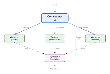
Empirical evidence.
The Orchestrator-Worker pattern has demonstrated striking gains across diverse domains. Anthropic's multi-agent research system [22] deployed a lead agent (the orchestrator) that coordinated multiple “sub-agent” workers for parallel web research, achieving a 90.2% improvement in research quality over a single-agent baseline on internal evaluation benchmarks. The key was not merely parallelism (running the same agent three times in parallel yields only modest improvements through majority voting) but specialised decomposition: the orchestrator assigned different sub-topics to different workers, each of which could focus its full context window on a narrow sub-problem.
Formally, the Orchestrator-Worker pattern instantiates Definition 25 with a specific structure. The orchestrator maintains an internal task plan that pairs instructions with assigned workers. At each step, the orchestrator:
Analyses the current state: examines completed results, identifies remaining sub-tasks, and detects failures or quality issues.
Selects the next worker and crafts the instruction with precisely the context that worker needs, no more, no less.
Dispatches the instruction to the worker and awaits the result.
Integrates the worker's output into the running solution, updating the task plan as needed.
Evaluates whether the task is complete () or whether further iterations are needed ().
This loop is illustrated in Figure 18. The orchestrator's effectiveness depends critically on the quality of the instructions it generates, a problem we formalise next under the name context engineering.
Context Engineering
The term context engineering was crystallised by OpenAI's engineering team in their description of the “harness” that surrounds and coordinates agent systems [24]. The core insight is that the primary bottleneck in multi-agent systems is not the capability of individual agents but the quality of the information they receive. A brilliant coder given a vague specification will produce mediocre code; the same coder given a precise specification, relevant examples, and clear constraints will produce excellent code. The orchestrator's job is to be the brilliant specification writer.
Definition 26 (Context Engineering).
Let be the full conversation history at step and let be the agent selected for execution. A context engineering function is a mapping (Context ENG) where is the space of raw task descriptions and is the space of engineered contexts (the actual prompt seen by the agent). The function performs:
Selection: choosing a relevant subset of the history, discarding messages irrelevant to agent 's sub-task;
Compression: summarising long message sequences into concise representations, reducing token count while preserving essential information;
Structuring: organising the selected information into a format matched to 's capabilities (e.g., code blocks for a coder agent, bullet points for a planner agent);
Augmentation: adding task-relevant context not present in the history, such as retrieved documentation, schema definitions, examples, or explicit constraints.
The engineered context is the instruction passed to the worker in Definition 25.
Entropy management.
OpenAI's characterisation of the harness as managing “entropy” in the information flow [24] can be formalised as follows. Let denote the Shannon entropy of the engineered context viewed as a random variable over possible instructions. A poorly designed context function produces high-entropy instructions (vague, ambiguous, containing irrelevant information), forcing the agent to resolve uncertainty internally, consuming reasoning tokens on disambiguation rather than problem-solving. A well-designed context function produces low-entropy instructions (precise, unambiguous, focused), allowing the agent to allocate its full reasoning budget to the sub-task.
Formally, let be the output of agent given context , and let denote the quality metric. We seek to maximise . By the data-processing inequality, (DATA Processing) where is any post-processing of . The first inequality tells us that the mutual information between context quality and the final output is bounded by the information in the context itself, underscoring that no amount of agent capability can compensate for information lost during context engineering. The orchestrator should therefore maximise by ensuring that task-relevant information is preserved in the engineered context.
Token Economics of Orchestration
Orchestration is not free. Every message the orchestrator sends, every context it engineers, every synthesis step it performs consumes tokens. Understanding the economics of token usage is essential for designing efficient multi-agent systems.
Kim et al. [19] conducted a systematic study of multi-agent LLM teams and arrived at a striking finding: token usage explains approximately 80% of the variance in task performance. Systems that used more tokens, by generating longer reasoning chains, producing more detailed sub-task instructions, or performing additional verification rounds, consistently outperformed systems that were more parsimonious, after controlling for model capability.
Proposition 13 (Token Usage Predicts Performance).
Let be a multi-agent system operating on a task distribution . Define the total token usage as (Total Tokens) where counts tokens consumed by the orchestrator (planning, routing, synthesis) and counts tokens consumed by worker (reasoning, generation, tool calls). Then, under the empirical model of [19], the system performance satisfies the regression (Token Regression) where is a diversity measure over agent capabilities, are regression coefficients, and captures residual variance. The coefficient of determination satisfies , with the term accounting for the dominant share of explained variance.
Proof sketch.
The logarithmic dependence on token count follows from an information-theoretic argument. Each token carries at most bits of information, where is the vocabulary. For a task requiring bits of “solution information” (a measure of the task's intrinsic complexity), the system must generate at least tokens. In practice, redundancy in natural language means the effective information per token is bits, so the required token count is . Performance improves as increases because additional tokens enable:
More thorough reasoning: longer chains of thought explore more solution paths (cf. the tree-search analysis in 23);
Better context engineering: the orchestrator can provide more detailed instructions, reducing worker uncertainty;
Verification and correction: additional tokens are spent on reviewing and revising worker outputs, catching errors that a single pass would miss.
The logarithmic (rather than linear) dependence reflects diminishing returns: the first tokens address the most important aspects of the task, while later tokens yield progressively smaller marginal gains. The diversity term captures the benefit of specialisation: a team of identical agents wastes tokens on redundant exploration, while a diverse team covers more of the solution space per token spent. Kim et al. [19] validated this model across 144 multi-agent configurations, finding with token usage as the dominant predictor.
Caution.
Token usage is not a free lunch. The token–performance relationship of Proposition 13 should not be interpreted as “more tokens always means better performance.” The relationship is logarithmic: doubling the token budget yields a constant additive gain, not a multiplicative one. Moreover, the cost of LLM inference scales linearly in token count, so the cost–performance frontier exhibits severely diminishing returns. In practice, the optimal operating point balances marginal performance gain against marginal cost, a classic economic optimisation. The orchestrator's role is to allocate tokens efficiently: spending more on high-value sub-tasks (complex reasoning, ambiguous specifications) and less on routine operations (formatting, simple lookups).
The MALLM Configuration Space
How many meaningfully different multi-agent systems can one build? The MALLM (Multi-Agent Large Language Model) framework of Becker et al. [23] answers this question by identifying four orthogonal design axes, each with a discrete set of options. The cross-product of these axes defines a configuration space whose size reveals the combinatorial richness of orchestration design.
Definition 27 (MALLM Configuration Space).
The MALLM configuration space is a 4-tuple where:
is the set of personas (role descriptions assigned to agents, e.g., “domain expert”, “devil's advocate”, “summariser”);
is the set of generators (the underlying LLM or LLM configuration used by each agent, e.g., GPT-4, Claude, Llama 3);
is the set of interaction paradigms (the communication structure, e.g., sequential debate, parallel brainstorm, hierarchical delegation);
is the set of decision mechanisms (the aggregation rule for combining agent outputs, e.g., majority vote, weighted average, LLM-as-judge).
A configuration is a 4-tuple . The total number of configurations is (Mallm SIZE) In the experiments of [23], the axes had sizes , , , , yielding distinct configurations.
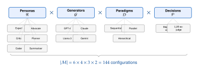
Navigating the configuration space.
The 144 configurations in Definition 27 may seem modest, but they represent only the coarse-grained design choices. Fine-grained decisions, such as the specific wording of persona prompts, the temperature and top- settings for each generator, the number of rounds in a debate paradigm, the prompt given to the LLM judge, each add further degrees of freedom. The effective design space is therefore far larger than 144, and manual exploration is infeasible.
Becker et al. [23] addressed this by running all 144 configurations on a common benchmark suite, enabling a factorial analysis that decomposes performance variance into contributions from each axis and their interactions. Key findings include:
Persona Paradigm interaction dominates. The choice of persona has the largest main effect, but its impact depends strongly on the interaction paradigm: a “devil's advocate” persona is highly effective in sequential debate but adds noise in parallel brainstorming.
Generator matters less than expected. Swapping the underlying LLM from GPT-4 to Claude or Llama 3 changed performance by less than the effect of the best versus worst persona assignment, suggesting that how agents are orchestrated matters more than which model powers them.
Decision mechanism interacts with task type. Majority voting excels on tasks with verifiable answers (e.g., coding, mathematics), while LLM-as-judge is superior for open-ended generation (e.g., creative writing, research synthesis).
These findings reinforce a central theme of this chapter: the protocol, how agents are organised and coordinated, often matters more than the raw capabilities of the individual agents.
Example 8 (Choosing an Orchestration Configuration).
Consider a software engineering task: given a GitHub issue, produce a patch that resolves the issue and passes the repository's test suite. Using the MALLM framework, one might select:
Personas: Coder (primary implementation), Reviewer (code quality), Planner (task decomposition), a subset .
Generator: The most capable available model (e.g., Claude or GPT-4), .
Paradigm: Hierarchical delegation, with the Planner as orchestrator and Coder/Reviewer as workers, .
Decision: LLM-as-judge (the orchestrator evaluates whether the patch is acceptable), .
This configuration mirrors the architecture that achieved state-of-the-art results on SWE-bench [22], confirming that principled configuration selection can recover empirically successful designs.
Orchestration as the Key Differentiator
Insight.
Orchestration is the key differentiator in multi-agent systems. The evidence from Anthropic's research system (90.2% improvement via orchestrated delegation) [22], OpenAI's harness framework (context engineering as the primary lever) [24], Kim et al.'s token analysis (80% variance explained by usage patterns) [19], and the MALLM factorial study (persona paradigm interaction dominates raw model choice) [23] all converge on a single conclusion: the way agents are orchestrated, who does what, with what information, in what order, matters more than the individual capability of any agent. This is the multi-agent analogue of a familiar insight from software engineering: system architecture matters more than component quality. A mediocre database with a brilliant query optimiser will outperform a brilliant database with a mediocre query optimiser. Likewise, a well-orchestrated team of capable (but not extraordinary) LLMs will outperform a poorly orchestrated team of frontier models. The practical implication is clear: invest in orchestration design before investing in more powerful models.
Formal Comparison of Orchestration Patterns
We can now compare the orchestration patterns encountered in this chapter through the lens of the MALLM configuration space and the token-performance model.
| Pattern | Control | Parallelism | Token cost | Best for |
| Round-robin | Decentralised | None | Low | Simple debates |
| Star (hub-and-spoke) | Centralised | None | Medium | Q&A routing |
| Orchestrator-Worker | Centralised | High | High | Complex tasks |
| Hierarchical | Multi-level | Medium | High | Large codebases |
| Swarm (peer-to-peer) | Decentralised | High | Variable | Exploration |
Table 4 summarises five common patterns. The choice among them depends on the task structure:
Decomposable tasks with independent sub-problems favour the Orchestrator-Worker pattern, which can assign sub-tasks in parallel and aggregate results.
Sequential reasoning tasks (e.g., mathematical proofs, multi-step plans) favour round-robin or sequential debate, where each agent builds on the previous agent's output.
Large-scale systems with hierarchical structure (e.g., a codebase with modules, packages, and files) favour hierarchical orchestration, where top-level orchestrators delegate to sub-orchestrators.
Open-ended exploration tasks (e.g., brainstorming, creative generation) favour swarm patterns where agents explore diverse directions without central coordination.
In each case, the orchestrator's design determines the efficiency frontier: the maximum performance achievable for a given token budget. The token–performance model of Proposition 13 provides a quantitative framework for comparing patterns: given two orchestration strategies and , the preferred strategy is the one achieving higher performance at equal token cost, or equivalently, the one achieving equal performance at lower cost.
Toward Game-Theoretic Foundations
The orchestration patterns developed in this section assume a cooperative setting: all agents share a common objective, and the orchestrator has full authority to assign tasks and evaluate outputs. But many real-world multi-agent deployments involve agents with heterogeneous objectives: LLMs fine-tuned by different organisations, agents representing different stakeholders, or adversarial agents injected to test system robustness.
When agent objectives diverge, the orchestrator can no longer assume that workers will faithfully execute instructions. A worker might “defect” by producing minimal-effort outputs to conserve its own token budget, or by subtly steering the conversation toward its own objective. The orchestrator must then design incentive-compatible mechanisms: protocols where each agent's self-interested behaviour aligns with the system's collective objective.
This is precisely the domain of game theory and mechanism design. In the next sections, we develop the game-theoretic foundations needed to analyse these strategic interactions: normal-form games and Nash equilibria, repeated games and the folk theorem (which shows how cooperation can emerge from repeated interaction even among self-interested agents), mechanism design (which shows how to construct protocols that make truthful behaviour optimal), and the Shapley value (which provides a principled method for assigning credit to agents based on their marginal contributions). The orchestrator's role evolves from a benevolent coordinator in the cooperative setting to a mechanism designer in the strategic setting, a transition that captures much of the mathematical richness of multi-agent AI.
Game Theory Foundations for Multi-Agent Systems
When multiple autonomous agents share an environment, the outcome experienced by any single agent depends not only on its own actions but also on the actions of every other agent. This fundamental interdependence is precisely the setting studied by game theory, the mathematical framework for analysing strategic interactions among rational decision-makers. In this section we develop the game-theoretic foundations needed to understand multi-agent LLM systems: normal-form games and Nash equilibria (Normal-Form Games), repeated games and the folk theorem (Repeated Games and Folk Theorems), mechanism design (Mechanism Design), and cooperative game theory with the Shapley value (Cooperative Game Theory and the Shapley Value).
The results in this section are classical, but their application to LLM-based agents is novel: each “player” is a language model instance with a policy , and the “actions” are the responses the model generates. The payoffs arise from task rewards, human evaluations, or other agents' reactions.
Historical Note.
From von Neumann to algorithmic game theory. The mathematical study of strategic interaction began with von Neumann's minimax theorem (1928) [25] and the landmark treatise Theory of Games and Economic Behavior (1944) [26] by von Neumann and Morgenstern, which established the field of game theory. John Nash's equilibrium concept (1950) [4] provided the central solution concept for non-cooperative games. Lloyd Shapley introduced the value bearing his name in 1953 [5], solving the problem of fair division in cooperative games. The 2000s brought algorithmic game theory [27], which studies computational aspects of game-theoretic solutions, a perspective directly relevant to multi-agent AI systems where equilibria must be computed, not merely shown to exist.
Normal-Form Games
The simplest and most widely used model of strategic interaction is the normal-form game, also called a strategic-form game.
Definition 28 (Normal-Form Game).
A normal-form game is a tuple where:
is a finite set of players (agents);
is the finite action set (or strategy space) of player ; the joint action space is ;
is the utility function (or payoff function) of player , mapping every joint action profile to a real-valued payoff.
A pure strategy for player is a deterministic choice . A mixed strategy is a probability distribution over . Under mixed strategies, the expected utility of player is (Expected Utility) We write for the strategy profile of all players except .
The central solution concept for non-cooperative games is the Nash equilibrium: a strategy profile from which no player can unilaterally improve their payoff.
Definition 29 (Nash Equilibrium).
A strategy profile is a Nash equilibrium (NE) of if for every player and every strategy , (NASH Condition) Equivalently, is a best response to for every player . A Nash equilibrium in which every is a pure strategy is called a pure-strategy Nash equilibrium; otherwise it is a mixed-strategy Nash equilibrium.
Example 9 (Prisoner's Dilemma).
The Prisoner's Dilemma is the archetypal multi-agent tension. Two agents simultaneously choose to Cooperate (C) or Defect (D), with the payoff matrix shown in fig:agents:prisoners-dilemma. The unique Nash equilibrium is with payoffs , even though both players would prefer the cooperative outcome with payoffs . This captures the fundamental tension in multi-agent systems: individually rational behaviour can lead to collectively suboptimal outcomes.
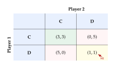
The most fundamental existence result in game theory guarantees that every finite game possesses at least one Nash equilibrium in mixed strategies.
Theorem 7 (Nash Equilibrium Existence).
Every finite game possesses at least one mixed-strategy Nash equilibrium.
Proof.
We provide a proof sketch using Kakutani's fixed-point theorem, which generalises Brouwer's theorem to set-valued (correspondence) maps.
Step 1: Define the strategy space. The mixed strategy set of each player is , the simplex over . This is a compact, convex, non-empty subset of . The joint strategy space is likewise compact and convex.
Step 2: Define the best-response correspondence. For each player and opponent profile , define (BEST Response) Since is linear in and is compact and convex, the set is non-empty, convex, and compact. Define the joint best-response correspondence by
Step 3: Verify Kakutani's conditions. The correspondence maps the compact convex set into itself. For each , the set is non-empty and convex (as a product of non-empty convex sets). By Berge's maximum theorem, has a closed graph (is upper hemicontinuous), since is continuous in all strategies.
Step 4: Apply Kakutani's fixed-point theorem. By Kakutani's theorem, there exists such that . This means that for every player , is a best response to , which is precisely the definition of a Nash equilibrium.
Remark 12 (Computational Complexity of Nash Equilibria).
While Nash equilibria are guaranteed to exist, finding them is computationally hard in general. The problem of computing a Nash equilibrium is PPAD-complete [28], meaning it is unlikely to admit a polynomial-time algorithm. For two-player games, the Lemke–Howson algorithm [29] finds a Nash equilibrium in exponential time in the worst case. For multi-agent LLM systems, this computational intractability suggests that agents will typically converge to approximate equilibria rather than exact ones.
Repeated Games and Folk Theorems
In many multi-agent LLM deployments, agents interact not once but repeatedly over multiple rounds; for instance, a coding assistant and a reviewer exchanging feedback over several iterations, or debate agents engaging in multiple rounds of argumentation. The theory of repeated games shows that such sustained interaction fundamentally changes the strategic landscape: cooperation can emerge as an equilibrium even in games where it is impossible in a single round.
Consider a stage game played infinitely often. In each period , the players simultaneously choose actions , observe the joint action profile , and receive stage payoffs . Each player maximises the discounted sum (Discounted Payoff) where is the discount factor. The normalisation by ensures that is a weighted average of stage payoffs, making it comparable in scale to the single-stage payoffs .
A strategy in the repeated game is a function mapping the entire history of play to a current action. The minimax payoff of player is (Minimax) the lowest payoff that the other players can force upon .
A payoff vector is feasible if it lies in the convex hull of the set of achievable payoff vectors, i.e., . A feasible payoff vector is individually rational if for all .
Theorem 8 (Folk Theorem for Repeated Games).
Let be a finite normal-form game, and let be any feasible and individually rational payoff vector (i.e., for all ). Then there exists such that for all , the payoff vector can be sustained as a Nash equilibrium payoff of the infinitely repeated game with discount factor .
Proof.
We construct an explicit equilibrium strategy profile using the grim trigger mechanism.
Step 1: Target action profile. Since is feasible, there exists a (possibly mixed) action profile (or a convex combination of pure profiles) such that for each . For simplicity, assume is a pure profile; the argument extends to correlated mixtures by standard techniques.
Step 2: Grim trigger strategy. Each player plays the following strategy :
Cooperative phase: play as long as all players have played in every previous round.
Punishment phase: if any player has ever played in some past round, switch to the minimax strategy against all deviators and play it forever.
Step 3: No profitable deviation. Suppose player considers deviating in period while all other players follow . The best single-period payoff from deviating is at most . After deviating, player receives at most in every subsequent period (since all opponents switch to minimax punishment). The payoff from deviating is therefore at most (Deviation Payoff) The payoff from cooperating forever is . Cooperation is incentive-compatible when , i.e., (FOLK IC) Rearranging, Since by assumption, the right-hand side is strictly less than 1. Setting ensures that cooperation is a best response for every player whenever .
Step 4: Subgame considerations. The grim trigger profile is a Nash equilibrium of the repeated game for . One can strengthen this to a subgame perfect equilibrium by replacing permanent punishment with more sophisticated strategies (e.g., mutual punishment phases of finite length), but the Nash equilibrium version suffices for our purposes.
Key Idea.
Repetition enables cooperation. The folk theorem has a striking implication for multi-agent LLM systems: when agents interact repeatedly with sufficient patience ( close to 1), any individually rational outcome, including full cooperation, can be sustained as an equilibrium. This provides a theoretical foundation for the empirical observation that LLM agents in iterative frameworks (debate, iterative refinement, multi-turn negotiation) converge to cooperative behaviours even when a single-round analysis would predict defection.
Mechanism Design
While game theory analyses the behaviour of agents within a fixed set of rules, mechanism design tackles the inverse problem: how should we design the rules of interaction so that self-interested agents produce a desired outcome? This is directly relevant to multi-agent LLM systems, where the system designer chooses the communication protocol, reward structure, and coordination rules.
Definition 30 (Mechanism Design).
A mechanism design problem consists of:
A set of agents with private types (unknown to the designer);
An outcome space ;
A social choice function specifying the designer's desired outcome for each type profile.
A mechanism specifies a message space for each agent and an outcome function . The mechanism implements if there exists an equilibrium in which each agent's message reveals enough information to compute .
A mechanism is incentive compatible (IC) if truth-telling is an equilibrium strategy: for each agent and each type profile , (IC) A mechanism is individually rational (IR) if every agent receives at least their outside option: for all .
The most celebrated incentive-compatible mechanism is the Vickrey–Clarke–Groves (VCG) mechanism.
Definition 31 (VCG Mechanism).
In the VCG mechanism, each agent reports a valuation function (ideally , the true valuation). The mechanism:
Chooses the outcome maximising social welfare: ;
Charges each agent the Clarke pivot payment: (VCG Payment) where is the outcome that would maximise welfare if agent were absent.
The agent's total utility is .
Proposition 14 (VCG Incentive Compatibility).
In the VCG mechanism, truth-telling () is a dominant strategy for every agent .
Proof.
Under truth-telling, agent 's total utility is (VCG Utility) The second term does not depend on agent 's report. Therefore, agent maximises its utility by maximising the first term, which is exactly what happens when the mechanism selects the socially optimal outcome using the true valuations. Hence truth-telling is a dominant strategy.
Remark 13 (Mechanism Design for Multi-Agent LLMs).
In multi-agent LLM systems, the “types” correspond to each agent's private information (e.g., specialised knowledge, confidence in an answer, computational budget), and the “mechanism” is the orchestration protocol. VCG-inspired designs can incentivise agents to truthfully report their confidence or capability, enabling the orchestrator to allocate tasks optimally. For instance, in a mixture-of-agents system, each model could report its estimated probability of success on a task; a VCG-like mechanism would ensure that no model benefits from over- or under-reporting its capability.
Cooperative Game Theory and the Shapley Value
In many multi-agent settings, agents form coalitions and the relevant question is not “what will each agent do?” but “how much does each agent contribute?” Cooperative game theory provides the mathematical framework for this analysis.
Definition 32 (Characteristic Function Game).
A characteristic function game (or coalitional game) is a pair where is the set of players and is the characteristic function satisfying . For any coalition , the value represents the total payoff that the members of can guarantee themselves, regardless of the actions of players outside .
Definition 33 (Shapley Value).
The Shapley value of player in the game is (Shapley Value) The term is the marginal contribution of player to coalition . The combinatorial weight equals the probability that is exactly the set of players preceding in a uniformly random permutation of . Thus is the expected marginal contribution of player over all possible orderings.
The Shapley value is not merely one of many possible allocation rules; it is the unique rule satisfying four natural fairness axioms.
Theorem 9 (Shapley Value Uniqueness).
The Shapley value is the unique function satisfying the following axioms:
Efficiency: ;
Symmetry: if players and are interchangeable (i.e., for all ), then ;
Linearity: for all games and scalars ;
Null player: if for all (player never contributes), then .
Proof.
The proof proceeds in three stages: we decompose any game into a basis of unanimity games, determine the unique Shapley value for each basis element, and reconstruct the general formula by linearity.
Step 1: Unanimity games form a basis. For any non-empty coalition , define the unanimity game by (Unanimity GAME) The set forms a basis for the vector space of all characteristic functions (with ). This can be verified by checking that these functions are linearly independent. Therefore, any game can be uniquely written as (Unanimity Decomposition) where the coefficients are the Harsanyi dividends, given by the Möbius inversion formula .
Step 2: Uniqueness for unanimity games. Consider the unanimity game . By the null player axiom, for all , since such players never contribute ( whenever ).
By the symmetry axiom, all players in receive the same value: for all , since any two members of are interchangeable in .
By the efficiency axiom, . Since only the players in receive nonzero values, and they all receive the same value, we conclude (Shapley Unanimity) This is uniquely determined by the three axioms (efficiency, symmetry, null player).
Step 3: Reconstruction by linearity. By the linearity axiom and the decomposition , (Shapley FROM Dividends) Since the decomposition is unique and each is uniquely determined, is uniquely determined.
Step 4: Verification. It remains to verify that the formula satisfies all four axioms. Efficiency: summing over all and exchanging the order of summation yields (a standard combinatorial identity). Symmetry, null player, and linearity are immediate from the formula.
Example 10 (Credit Assignment in a Multi-Agent Coding Team).
Consider three LLM agents, a Coder (), a Reviewer (), and a Tester (), collaborating to solve a programming task. Define the characteristic function (performance score out of 100): Computing the Shapley value for the Coder: Similarly, and , with , confirming efficiency. The Coder receives the largest share, reflecting its high marginal contributions across all coalitions.
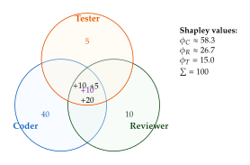
Consensus and Coordination
A recurring motif in multi-agent systems is the need for agents to agree: on an answer, a plan, a diagnosis, or a value. When agents begin with different opinions, how do they converge? How fast? And does the converged opinion bear any relation to the truth?
This section develops the mathematical theory of consensus. We begin with graph-Laplacian consensus (Graph Laplacian Consensus), where agents iteratively average their neighbours' values and provably converge to the global mean. We then apply consensus theory to agent opinions (Consensus in Agent Opinions), connecting to recent empirical findings that LLM agents spontaneously adopt averaging protocols. The Condorcet jury theorem (Condorcet Jury Theorem) quantifies when majority voting among agents outperforms any individual, while the analysis of quality versus diversity (Quality vs. Diversity) reveals the surprising empirical finding that agent quality dominates agent diversity.
Graph Laplacian Consensus
Consider agents arranged on a communication graph with . Each agent holds a scalar state at time . Agents can communicate only with their neighbours in .
Definition 34 (Graph Laplacian).
Let be an undirected graph with adjacency matrix (where if and otherwise) and degree matrix . The graph Laplacian is the matrix . Key properties of :
is symmetric and positive semidefinite;
(the all-ones vector is in the null space);
The eigenvalues satisfy ;
if and only if is connected; is called the Fiedler eigenvalue or algebraic connectivity of .
The continuous-time consensus protocol asks each agent to move towards the average of its neighbours: (Continuous Consensus) which in component form reads , where is the neighbourhood of agent .
Theorem 10 (Consensus Convergence).
Proof.
The solution of the linear ODE is . Since is symmetric, it has an orthonormal eigenbasis with corresponding eigenvalues (the strict inequality holds because is connected). We choose .
Step 1: Eigenbasis decomposition. Expand the initial condition in the eigenbasis: (Eigenbasis Expansion) Then (Consensus Evolution)
Step 2: The consensus component is preserved. The coefficient along is . Since , this component is preserved for all time: .
Step 3: All other components decay. For , the term decays exponentially since . Therefore, (Consensus Residual) Taking norms and using orthonormality of the eigenbasis, (Consensus Bound) Taking square roots yields . Since , the bound converges to zero, establishing .
Remark 14 (Discrete-Time Consensus).
The discrete-time analogue replaces the ODE with the iteration (Discrete Consensus) where is a step size satisfying to ensure convergence. The optimal step size minimises the spectral radius of , yielding the fastest convergence rate of . Alternatively, one can use the Metropolis–Hastings weight matrix for , which is doubly stochastic by construction and does not require knowledge of global graph properties.
Consensus in Agent Opinions
In multi-agent LLM systems, each agent holds not a scalar value but a distribution over possible answers. Let be agent 's opinion vector, where is a discrete set of candidate answers. A natural consensus protocol is (Opinion Consensus) where is a doubly stochastic weight matrix respecting the communication graph. This protocol converges to for all , exactly as in the scalar case.
Chen et al. [71] observed that LLM agents engaged in multi-round deliberation spontaneously adopt protocols resembling : after exchanging messages, agents update their answers in a direction that averages the positions of their conversational partners. The Fiedler eigenvalue of the communication graph determines the convergence speed: sparse networks (small ) converge slowly, while dense networks (large ) converge quickly but may suppress diversity prematurely.
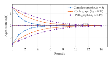
Condorcet Jury Theorem
A fundamental question in multi-agent systems is: when does aggregating the outputs of multiple agents improve upon any individual? The oldest and most elegant answer comes from the Marquis de Condorcet (1785).
Theorem 11 (Condorcet Jury Theorem).
Let independent agents each have probability of choosing the correct answer to a binary question. The probability that a majority vote yields the correct answer satisfies (Condorcet Limit) where is the indicator that agent is correct. Moreover, is strictly increasing in (for odd ).
Proof.
Let , where are independent Bernoulli random variables with parameter . Then and .
Majority vote is correct when . Standardising, (Condorcet Standardise) Let denote the standardised sum. By the central limit theorem, as .
The threshold on the right-hand side is (Condorcet Threshold) Since , the numerator , so as . Therefore, (Condorcet Conclusion) This completes the proof that .
The monotonicity claim (for odd ) follows from a direct combinatorial argument: adding two agents with accuracy to an existing panel of odd size strictly increases the majority accuracy, since the probability that both new agents are wrong () is less than the probability that both are right ().
This result has been invoked under the slogan “More Agents Is All You Need” [30]: simply sampling multiple responses from an LLM and taking a majority vote can substantially boost accuracy. However, the theorem's independence assumption is critical and often violated in practice.
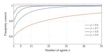
Example 11 (Five Agents Solving a Math Problem).
Suppose five independent LLM agents each have probability of correctly solving a given math problem. Under majority vote, the probability that at least three out of five are correct is (FIVE Agents CALC) Thus majority voting boosts accuracy from to approximately . With agents at the same individual accuracy, .
Quality vs. Diversity
The Condorcet theorem assumes independent agents, but LLM agents trained on similar data exhibit strong correlations in their errors. This subsection analyses how correlation degrades the Condorcet guarantee and examines whether diversity or quality matters more.
Proposition 15 (Correlated Agents Break Condorcet).
Let be identically distributed indicators with and pairwise correlation for all . Then the effective number of independent agents is (N EFF) and for sufficiently large , even as , destroying the Condorcet guarantee.
Proof.
Let and . We have and An independent sample of size would have variance . Equating, As , . Therefore, if , then regardless of the number of agents, which is insufficient for majority voting to reliably outperform an individual.
Proposition 16 (Quality Dominates Diversity).
Consider a multi-agent system with agents. Under a simple bias-variance decomposition, the ensemble error can be written as (BIAS Variance) where is the average squared bias of individual agents, is the average variance, and is the average pairwise correlation. Quality improvements (reducing ) contribute linearly, while diversity improvements (reducing ) contribute only through the variance term, which is already reduced by the factor. Empirically, is the dominant source of error across standard benchmarks [30], leading to the finding that Self-MoA (repeatedly sampling from the best model) outperforms Mixed-MoA (mixing different models of varying quality).
Key Idea.
Quality of individual agents matters more than their number. While the Condorcet jury theorem suggests that adding more agents always helps, this relies on the independence assumption. In practice, LLM agents share training data and exhibit correlated errors (). The effective number of independent agents is , which saturates quickly. Improving the quality of each agent (reducing bias) yields larger gains than increasing the number of correlated agents (reducing variance through diversity). As a practical guideline: invest in better individual agents before scaling the number of agents.
Cooperation and Competition
The game-theoretic framework of Game Theory Foundations for Multi-Agent Systems predicts equilibrium behaviour under the assumption of full rationality. But LLM agents are not perfectly rational: they are shaped by pretraining data, in-context examples, and prompt instructions, all of which introduce biases that can push behaviour away from Nash equilibrium. This section examines how cooperation and competition emerge in practice when LLM agents interact, revealing surprising phenomena that classical game theory does not predict.
Spontaneous Cooperation in LLM Agents
One of the most striking findings in multi-agent LLM research is that agents placed in competitive game-theoretic settings often spontaneously cooperate [31], even when the one-shot Nash equilibrium prescribes defection.
Definition 35 (Tacit Collusion).
Tacit collusion occurs when agents coordinate on a cooperative outcome without explicit communication or agreement. Formally, let be a one-shot game with a unique Nash equilibrium and a cooperative outcome with for all . Tacit collusion occurs when agents converge to or a neighbourhood thereof, despite the absence of an explicit coordination mechanism.
Keynesian beauty contest.
In the Keynesian beauty contest, players simultaneously choose numbers . The winner is the player closest to of the average choice. Iterated elimination of dominated strategies yields the unique Nash equilibrium for all , since if all players choose , the optimal target is , and iterating this contraction drives the equilibrium to zero. Empirically, LLM agents converge to this equilibrium within – rounds of repeated play, demonstrating both the capacity for strategic reasoning and rapid learning from interaction [31].
Bertrand competition.
In the Bertrand duopoly, two firms simultaneously set prices for identical products; consumers buy from the cheaper firm. The unique Nash equilibrium is (marginal cost pricing, yielding zero profit). However, the cartel (collusive) outcome is (monopoly pricing), which maximises joint profit.
Example 12 (Bertrand Competition with LLM Agents).
When two LLM agents are placed in a repeated Bertrand game with marginal cost and monopoly price , they converge to prices between and , significantly above the Nash equilibrium of but below the full monopoly price [31]. This intermediate outcome represents partial tacit collusion: the agents exploit the repeated structure to sustain supra-competitive prices without explicit coordination.
The mechanism is instructive. Each agent's policy , conditioned on the history of previous price pairs, adapts in a manner consistent with tit-for-tat: if the opponent raised prices in the previous round, the agent reciprocates; if the opponent undercut, the agent retaliates. This behaviour emerges not from game-theoretic reasoning but from patterns in the pretraining data, where cooperative norms and reciprocity are pervasive.
Proposition 17 (Shared Priors Enable Implicit Coordination).
Let and be two LLM agents derived from the same pretrained model via different fine-tuning procedures. If the fine-tuning perturbation is small (i.e., for ), then the agents share an approximate common prior over strategies. Specifically, for any history , This shared prior enables implicit coordination: agents can predict each other's behaviour with high accuracy, enabling cooperative strategies that would require explicit communication between agents with uncorrelated priors.
Proof.
By the triangle inequality for KL divergence (using the chain rule for total variation distance and Pinsker's inequality), where the first two terms are bounded by the fine-tuning constraint and the cross term is bounded by .
Co-Player Inference and Predictive Policy Improvement
Beyond shared priors, LLM agents can perform in-context co-player inference: from observing an opponent's actions, the agent updates its belief about the opponent's strategy and adapts accordingly.
Definition 36 (Predictive Policy Improvement).
Let be a pretrained base policy and an estimated action-value function based on the opponent's inferred strategy. Predictive Policy Improvement (PPI) updates the agent's policy as (PPI) where is a temperature parameter controlling the degree of exploitation. The value incorporates the agent's prediction of the co-player's future actions, creating an implicit best-response dynamic.
The PPI framework reveals that cooperation can emerge through a diversity training mechanism: when agents are trained against a diverse population of opponents, they learn policies that are robust to variation in opponent behaviour. This robustness, combined with co-player inference, leads to mutual adaptation and ultimately cooperation [72]. The process can be formalised as convergence to a correlated equilibrium of the underlying game, which generically yields higher social welfare than Nash equilibrium.
Co-Evolution: The Red Queen Hypothesis
When agents in a multi-agent system simultaneously learn, the environment from each agent's perspective is non-stationary: every agent's reward landscape shifts as other agents update their policies. This gives rise to co-evolutionary dynamics: an arms race reminiscent of the Red Queen hypothesis in evolutionary biology.
Definition 37 (Co-Evolutionary Dynamics).
Consider agents with parameters . Each agent receives a reward that depends on all agents' parameters. The co-evolutionary dynamics are the coupled gradient ascent equations (Coevolution) The joint system defines a dynamical system on the product parameter space , with the joint gradient field .
Theorem 12 (Red Queen Equilibrium).
Suppose each reward function is twice continuously differentiable, -strongly concave in (for fixed ), and the cross-agent interaction gradients are bounded: for all . If (the self-improvement rate dominates the interaction effect), then:
Proof sketch.
Define the joint best-response map where , which is unique by -strong concavity.
For any two joint parameter vectors and , the -strong concavity and -bounded cross-derivatives imply (via the implicit function theorem for each best response) (Contraction STEP) Summing over and using the condition , (Contraction SUM) Since , is a contraction mapping on the product space. By the Banach fixed-point theorem, has a unique fixed point . The convergence rate follows from bounding the spectral radius of using the strong concavity parameter minus the interaction parameter .
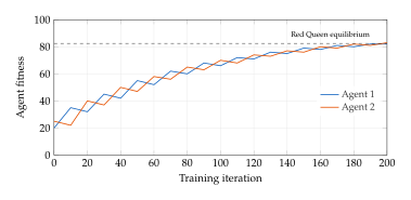
Distributed Problem Solving
While the preceding subsections demonstrate that LLM agents can cooperate in stylised game-theoretic settings, their performance on distributed combinatorial problems remains limited. Guo et al. [73] evaluated LLM agents on classic distributed computing tasks (graph colouring, vertex cover, leader election, and consensus) and found that:
Performance is reasonable at small scale ( agents) but degrades sharply as increases, with near-zero success rates at for most problems.
Three primary failure modes emerge: enumerate[(i)]
Strategy miscoordination: agents adopt incompatible local strategies that cannot be reconciled globally;
Uncritical trust: agents accept neighbours' proposals without verifying consistency, propagating errors;
Poor conflict resolution: when two agents disagree, neither has a principled mechanism for yielding, leading to oscillation or deadlock. enumerate
These failure modes are rooted in the architecture of LLM agents: they lack global state awareness (each agent sees only its neighbourhood), they have limited working memory for tracking negotiation history, and they lack formal verification mechanisms for checking global consistency. Addressing these limitations requires combining LLM agents with formal coordination protocols (see Scheduling, Load Balancing, and Fault Tolerance).
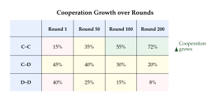
Credit Assignment in Multi-Agent Systems
When agents collaborate on a task and achieve a joint outcome, a fundamental question arises: how much did each agent contribute? This is the multi-agent credit assignment problem, and its solution is essential for training, rewarding, and improving individual agents within a team. Without proper credit assignment, agents may free-ride on others' contributions or be penalised for failures caused by their teammates.
This section develops the theory and algorithms for multi-agent credit assignment. We formalise the problem using counterfactual reasoning (The Multi-Agent Credit Assignment Problem), connect it to the Shapley value from Cooperative Game Theory and the Shapley Value and develop efficient approximation algorithms (Shapley Value Computation), introduce difference rewards as a practical alternative (Difference Rewards), and derive multi-agent policy gradient theorems that incorporate credit assignment (Credit Assignment for Agent Training).
The Multi-Agent Credit Assignment Problem
Definition 38 (Multi-Agent Credit Assignment).
Let be a set of agents that jointly produce a team outcome with value . The credit assignment problem asks: for each agent , what is the quantity representing agent 's contribution, subject to the constraint ?
The counterfactual contribution of agent is (Counterfactual) measuring how much the team outcome degrades if agent is removed. Note that in general due to complementarities and redundancies among agents.
The counterfactual approach is intuitive but flawed: it does not account for the order in which agents are removed, nor does it handle synergies between agents. The Shapley value (Definition 33) resolves both issues by averaging the marginal contribution over all possible orderings, yielding a unique, fair allocation that satisfies efficiency ().
Shapley Value Computation
The exact Shapley value requires summing over all subsets of , which is computationally intractable for large . The standard approach is Monte Carlo approximation: sample random permutations and average the marginal contributions.
Algorithm 3 (Monte Carlo Shapley Approximation).
Input: Value function oracle , number of samples . Output: Estimated Shapley values .
- Initialise for all .
- for
- Sample a uniformly random permutation of .
- .
- for
- -th player in the permutation
- return .
Proposition 18 (Shapley Approximation Guarantee).
Let be a bounded value function. The Monte Carlo Shapley approximation (Algorithm 3) with random permutations satisfies (Shapley Hoeffding) In particular, samples suffice to ensure for all simultaneously with probability at least .
Proof.
For a fixed agent , define the random variable where is the set of agents preceding in the -th random permutation. Then and (by the probabilistic interpretation of the Shapley value as the expected marginal contribution over random orderings).
Each satisfies (since takes values in ), so is bounded in an interval of length . By Hoeffding's inequality, (Hoeffding Application) Applying a union bound over all agents and setting the right-hand side to , we require .
Difference Rewards
An alternative to the Shapley value that avoids summing over exponentially many subsets is the difference reward, which uses a single counterfactual evaluation.
Definition 39 (Difference Rewards).
Let be a joint trajectory of agents, and let be the team reward. Define as the counterfactual trajectory in which agent is replaced by a default agent (e.g., a random policy or a null agent that takes no actions). The difference reward for agent is (Difference Reward)
Proposition 19 (Difference Reward Incentive Alignment).
If the team reward function factorises as where each depends on agent 's actions and the joint state, and if the default policy does not affect other agents' rewards (i.e., for ), then the gradient of the difference reward with respect to agent 's policy equals the gradient of the team reward: (DIFF Reward Gradient)
Proof.
Under the stated conditions, (DIFF Reward Expand) By the assumption that replacing agent with the default does not affect other agents' individual rewards, the summation over vanishes. Therefore, . The second term is a constant with respect to (it involves only the default policy for agent ), so , where the last equality uses the fact that the other terms in do not depend on .
Credit Assignment for Agent Training
Credit assignment becomes most important when we wish to train individual agents within a multi-agent system. The multi-agent policy gradient theorem provides the foundation for this.
Theorem 13 (Multi-Agent Policy Gradient).
Consider agents with policies , , acting in a shared environment with joint policy (conditional independence given the state). Let be the expected team reward. Then the gradient of with respect to agent 's parameters is (MA Policy GRAD) where is agent 's credit signal at time (which may be the Shapley value, difference reward, or any other estimator of agent 's contribution to the reward from time onward).
Proof.
Start from the standard policy gradient for the joint policy. The expected return is (J DEF) where the sum is over all possible trajectories and the trajectory probability factorises as (Trajectory PROB)
Taking the gradient with respect to , (LOG Trick) Now, in , only the terms involving depend on : (Score Function) This is because , and only the terms depend on . Substituting back, (Reinforce FULL) Replacing the full return with agent 's credit signal (which may be the Shapley value of agent 's contribution from time onward, or the difference reward ) is justified by the baseline subtraction lemma: replacing with any function that has the same gradient in expectation does not change the gradient but may reduce variance. This yields .
Example 13 (Credit Assignment in a Three-Agent Research Team).
Consider three LLM agents collaborating on a research task:
Agent A (Literature Surveyor): searches and summarises relevant papers;
Agent B (Hypothesis Generator): proposes hypotheses based on the survey;
Agent C (Experiment Designer): designs experiments to test hypotheses.
The team receives a quality score (out of 100) from a human evaluator. Ablation scores: , , , , , .
Computing Shapley values using the permutation formula: Verification: , confirming efficiency. The Literature Surveyor receives the largest credit, consistent with its high marginal contributions: the survey is the foundation on which hypotheses and experiments are built.
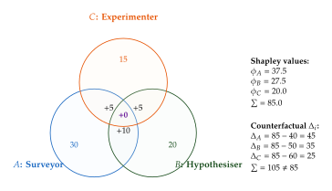
Scheduling, Load Balancing, and Fault Tolerance
A multi-agent system is only as effective as its ability to allocate tasks efficiently, balance computational loads, and recover gracefully from failures. These operational concerns are often overlooked in discussions of multi-agent intelligence, yet they determine whether a theoretically powerful multi-agent design can function in practice.
This section develops the mathematical foundations of three interconnected topics: task scheduling as combinatorial optimisation (Task Scheduling as Optimisation), online scheduling and load balancing (Online Scheduling and Load Balancing), and fault tolerance in the presence of adversarial or Byzantine agents (Fault Tolerance).
Task Scheduling as Optimisation
Definition 40 (Agent Scheduling Problem).
Given agents and tasks, the scheduling problem is to find an assignment mapping each task to an agent, with the objective of minimising the makespan, the time at which the last agent finishes: (Makespan) where is the cost (time) for agent to complete task . In the identical machines case, for all (task cost depends only on the task). In the unrelated machines case, varies arbitrarily with both and .
Even the simplest variant of this problem is computationally hard.
Proposition 20 (Scheduling NP-Hardness).
The makespan minimisation problem on identical machines is NP-hard.
Proof sketch.
We reduce from the Partition problem. Given a set of positive integers with sum , Partition asks whether there exists a subset with . Construct a scheduling instance with identical machines and tasks with costs . The makespan is exactly if and only if a partition exists. Since Partition is NP-complete, makespan minimisation on identical machines is NP-hard.
Despite NP-hardness, simple greedy algorithms provide provable approximation guarantees. The Longest Processing Time First (LPT) algorithm sorts tasks in decreasing order of cost and assigns each task to the least loaded machine, achieving a -approximation ratio [74]. For multi-agent LLM systems where task costs are estimated rather than known exactly, this greedy approach is both practical and near-optimal.
Remark 15 (Scheduling in Multi-Agent LLM Systems).
In a multi-agent LLM system, the “tasks” are sub-problems or queries, the “agents” are LLM instances (possibly with different capabilities), and the “cost” is the expected latency or token count for agent to process task . The orchestrator (see Definition 25) solves a variant of in real time, balancing completion time against the quality of each agent's output. This naturally extends to a bi-objective optimisation: minimise makespan while maximising output quality.
Online Scheduling and Load Balancing
In many practical settings, tasks arrive online and their costs are unknown a priori. We develop two key results: the power of randomised load balancing and the regret guarantees of online learning algorithms.
Balls into bins.
The simplest load-balancing model distributes tasks (“balls”) uniformly at random among agents (“bins”). The maximum load (number of tasks assigned to the busiest agent) determines the makespan.
Proposition 21 (Power of Two Choices).
Uniform allocation: If balls are thrown independently and uniformly into bins, the maximum load is with high probability.
Two-choice allocation: If each ball is placed in the less loaded of two independently and uniformly chosen bins, the maximum load drops to with high probability.
The exponential improvement from one to two choices is called the power of two choices [32].
Proof sketch for part (b).
We use a layered induction argument. Define as the number of bins with load . Under the two-choice protocol, a new ball increases the load of some bin from to only if both randomly chosen bins already have load . The probability of this event is at most .
For the base case, trivially. For the inductive step, the expected value of satisfies (TWO Choice Recursion) Starting from , we get , , until drops below 1. More precisely, if (which can be verified by induction using ), then when , i.e., . Therefore, the maximum load is with high probability.
Online scheduling with EXP3.
When task costs are adversarial (unknown and potentially chosen by an adversary), we can use the EXP3 (Exponential-weight algorithm for Exploration and Exploitation) algorithm from the adversarial multi-armed bandit literature. EXP3 maintains a probability distribution over agents and achieves a regret bound of over rounds with agents, where regret is measured against the best fixed agent in hindsight [75].
Algorithm 4 (EXP3 for Agent Selection).
Input: Number of agents , number of rounds , learning rate . Output: Agent selection sequence.
- Initialise weights for all .
- for
- Set probabilities:
- Select agent .
- Observe reward of selected agent.
- Compute importance-weighted estimate: if , else .
- Update weights: .
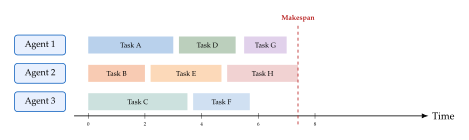
Fault Tolerance
In any distributed system, agents may fail: by crashing, producing incorrect outputs, or, in the worst case, behaving adversarially. This subsection addresses the fundamental limits of fault tolerance in multi-agent systems, culminating in the classical Byzantine consensus bound.
Definition 41 (Byzantine Fault Tolerance).
An agent is Byzantine if it may deviate from its prescribed protocol in an arbitrary and potentially adversarial manner: it may send conflicting messages to different agents, lie about its observations, or strategically manipulate the protocol to cause maximum disruption. A multi-agent protocol is -Byzantine fault tolerant if it achieves its specification (e.g., consensus) even when up to of the agents are Byzantine.
The foundational result of distributed computing establishes a sharp threshold for the number of Byzantine agents that can be tolerated.
Theorem 14 (Byzantine Consensus Bound).
No deterministic consensus protocol can tolerate Byzantine agents among total agents if . Equivalently, Byzantine consensus requires .
Proof.
We prove the impossibility direction: if , no deterministic protocol achieves consensus. The proof uses a partition argument due to Lamport, Shostak, and Pease [33].
Step 1: Partition into three groups. Partition the agents into three groups , each of size at most (possible since ).
Step 2: Construct two scenarios. Consider a binary consensus problem where each agent has an input and must output a decision satisfying:
Agreement: all non-Byzantine agents output the same decision;
Validity: if all non-Byzantine agents have the same input , the decision must be .
Scenario A: Agents in have input ; agents in have input ; agents in are Byzantine. The Byzantine agents in send messages to as if they had input , and to as if they had input .
Scenario B: Agents in have input ; agents in have input ; agents in are Byzantine. The Byzantine agents in behave exactly as did in Scenario A (sending the same messages as an honest with input 1).
Scenario C: Agents in have input ; agents in have input ; agents in are Byzantine. The Byzantine agents in behave exactly as did in Scenario A.
Step 3: Derive contradiction. In Scenario B, all non-Byzantine agents ( and ) have input , so the decision must be (by validity).
In Scenario C, all non-Byzantine agents ( and ) have input , so the decision must be (by validity).
Now consider agents in in Scenario A. From 's perspective:
The messages from are identical to those in Scenario B (since has input in both scenarios and receives the same messages from );
The messages from are identical to those in Scenario C (since has input in both scenarios and receives the same messages from ).
Therefore, cannot distinguish Scenario A from Scenario B (where the decision must be ) or from Scenario C (where the decision must be ). Since must commit to a single decision, it violates either the validity condition of Scenario B or Scenario C. This contradicts the assumption that the protocol achieves consensus with Byzantine faults when .
Remark 16 (Byzantine Faults in LLM Systems).
In multi-agent LLM systems, “Byzantine” behaviour arises from several sources: (a) adversarial prompt injection, where a malicious user manipulates one agent's input to corrupt its outputs; (b) model hallucination, where an agent produces confidently wrong outputs that mislead other agents; (c) self-replicating attacks (see Definition 42), where adversarial content propagates through the agent network. The Byzantine consensus bound implies that if more than one-third of agents in a system are compromised, no protocol can guarantee correct consensus, a sobering constraint for systems deployed in adversarial environments.
Definition 42 (CODES Attack).
A CODES (Cooperative and Distributed Evil Siblings) attack is a self-replicating adversarial prompt attack on multi-agent systems [34]. In a CODES attack:
An adversary crafts a prompt containing instructions for the receiving agent to (i) execute a malicious action, and (ii) propagate to its neighbours in the communication graph;
The attack spreads like a virus through the agent network: if agent is compromised at time , it sends to all agents , compromising them at time ;
The propagation follows the graph's structure: on a connected graph of diameter , the entire network is compromised within communication rounds.
Caution.
Multi-agent systems inherit and amplify single-agent vulnerabilities. A single compromised agent in a multi-agent system is far more dangerous than a single compromised standalone model. Through the communication network, one agent's failure can cascade to the entire system. The CODES attack demonstrates that adversarial prompts can self-replicate across agents, converting an vulnerability (one compromised agent) into an system-wide failure in rounds, where is the graph diameter. The Byzantine consensus bound (Theorem 14) shows that once more than agents are compromised, no deterministic protocol can recover correct consensus. Defence strategies must therefore focus on containing compromised agents (e.g., limiting communication rates, sandboxing untrusted outputs) rather than merely detecting them.
Example 14 (CODES Attack Propagation).
Consider a multi-agent system with agents arranged in a grid graph (each agent connected to its horizontal and vertical neighbours). The graph diameter is . Suppose agent (top-left corner) receives an adversarial prompt.
Round 0: Agent is compromised. . Byzantine tolerance holds.
Round 1: propagates the attack to its neighbours and . Now . Byzantine tolerance is exactly at the threshold.
Round 2: The attack reaches , , . Now . No deterministic consensus protocol can guarantee correctness.
Round 3–4: The remaining agents (, , ) are compromised. The entire system is under adversarial control.
The total time from initial compromise to complete system failure is 4 rounds (the graph diameter), regardless of the number of agents. This demonstrates the critical importance of fast detection and isolation mechanisms.
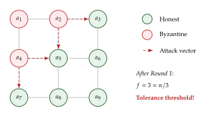
Practical fault tolerance in LLM systems.
The AgentScope framework [10] implements a four-tier fault tolerance strategy for multi-agent LLM systems:
Retry with backoff: failed API calls are retried with exponential backoff, tolerating transient failures;
Output validation: each agent's output is checked against format and content constraints before being passed to other agents;
Redundant execution: critical tasks are assigned to multiple agents, with outputs reconciled via majority vote (requiring for Byzantine tolerance);
Checkpoint and rollback: the system state is periodically checkpointed, allowing rollback to a consistent state after detecting a failure cascade.
These pragmatic mechanisms complement the theoretical bounds of Theorem 14, providing defence in depth against both accidental failures and adversarial attacks.
Insight.
The fault tolerance trilemma. Multi-agent LLM systems face a fundamental tension among three desiderata: (1) performance, which improves with more inter-agent communication and trust; (2) fault tolerance, which improves with redundancy and scepticism; and (3) efficiency, which degrades with both redundancy and verification overhead. The Byzantine bound quantifies the minimum cost of fault tolerance: tolerating even one Byzantine agent requires at least four agents, a overhead. For multi-agent LLM systems where each agent incurs significant computational cost (inference on a large model), this overhead may be prohibitive. Practical systems must therefore make explicit trade-offs: which agents are trusted? Which outputs require verification? What failure modes are acceptable? The answers depend on the deployment context and the cost of incorrect outputs.
Summary of Sections 11–15
This part of the chapter developed the mathematical foundations for multi-agent interaction, coordination, and operations. Game Theory Foundations for Multi-Agent Systems established game-theoretic foundations, from Nash equilibria through the folk theorem to Shapley values. Consensus and Coordination analysed consensus convergence, the Condorcet jury theorem, and the surprising dominance of quality over diversity. Cooperation and Competition examined how cooperation emerges spontaneously among LLM agents, connecting to co-evolutionary dynamics and the Red Queen hypothesis. Credit Assignment in Multi-Agent Systems formalised credit assignment and derived multi-agent policy gradients. Finally, Scheduling, Load Balancing, and Fault Tolerance addressed the operational concerns of scheduling, load balancing, and fault tolerance, culminating in the Byzantine consensus bound.
The recurring mathematical theme is the interplay between individual rationality and collective optimality. Nash equilibria may be socially suboptimal (Prisoner's Dilemma), but repetition enables cooperation (folk theorem). Majority voting improves upon individuals (Condorcet), but correlation limits the gains (Proposition 15). The Shapley value provides the unique fair allocation of credit, but is exponentially expensive to compute exactly. Byzantine agents can corrupt consensus, but agents suffice to tolerate failures.
These mathematical tools, drawn from game theory, graph theory, probability, and distributed computing, form the analytical backbone of multi-agent AI systems. The following sections (in the companion files) build on these foundations to address emergent behaviours, safety, and the future trajectory of multi-agent systems.
Exercise 4 (Nash Equilibrium in a Coordination Game).
Consider the Battle of the Sexes game with payoff matrix:
| Opera | Football | |
| Opera | ||
| Football |
Find all pure-strategy Nash equilibria.
Find the unique mixed-strategy Nash equilibrium. What is the expected payoff to each player?
Relate this to a multi-agent LLM system where two agents must agree on a common output format but have different preferences.
Exercise 5 (Folk Theorem Discount Factor).
In the Prisoner's Dilemma with payoffs as in fig:agents:prisoners-dilemma, compute the minimum discount factor such that mutual cooperation can be sustained as a Nash equilibrium of the infinitely repeated game using grim trigger strategies.
Exercise 6 (Shapley Value for Symmetric Agents).
Let be a symmetric game, meaning depends only on : for some function with . Show that the Shapley value of every player is .
Exercise 7 (Consensus on a Star Graph).
Consider agents on a star graph: agent 1 is connected to all other agents, and no other edges exist.
Compute the graph Laplacian and its eigenvalues.
What is the Fiedler eigenvalue ? How does the consensus convergence rate compare to a complete graph?
Discuss the implications for a multi-agent system with a central orchestrator (hub) connected to specialised agents (leaves).
Exercise 8 (Correlated Condorcet).
Ten LLM agents, each with individual accuracy , are used for majority voting. Their pairwise correlation is .
Compute the effective number of independent agents .
Estimate the majority-vote accuracy using the Condorcet formula with replacing .
How many agents with would be needed to match the performance of independent () agents?
Exercise 9 (Multi-Agent Credit Assignment).
Four LLM agents collaborate on a translation task. The characteristic function (BLEU score) is: ; for all ; for all pairs; for all triples; .
Compute the Shapley value of each agent. (Hint: use the symmetry of the game.)
Compute the counterfactual contribution of each agent. Do they sum to ?
If you can afford only random permutations for Monte Carlo Shapley estimation, what is the expected approximation error (use Proposition 18)?
Exercise 10 (Byzantine Fault Tolerance Threshold).
A multi-agent system has agents.
What is the maximum number of Byzantine agents that a deterministic consensus protocol can tolerate?
If agents are arranged on a cycle graph and a CODES attack starts at one agent, after how many rounds does the number of compromised agents exceed the Byzantine tolerance threshold?
Propose a modification to the communication protocol that would slow the propagation of a CODES attack.
Exercise 11 (Power of Two Choices).
A system has agents and incoming tasks.
Under uniform random assignment, estimate the maximum load using the bound.
Under the power-of-two-choices protocol, estimate the maximum load using the bound.
If each “load unit” corresponds to a 30-second LLM inference call, estimate the wall-clock time savings from using two-choice assignment versus uniform assignment.
Evolutionary Approaches to Agent Systems
Nature solved the design problem long before engineers did. Biological evolution (blind variation coupled with selective retention) produced the staggering diversity of life on Earth without a single line of pseudocode. The same principle applies to the design of agentic AI systems: rather than hand-crafting the architecture of a multi-agent system, we can evolve it. This section develops the mathematical foundations of evolutionary approaches to agent design, from swarm-intelligence-based architecture search to trajectory-level self-improvement to population dynamics that explain how specialisation emerges in agent ecosystems.
The intellectual arc is as follows. We begin with SwarmAgentic (Agent Architecture Search via Swarm Intelligence), which adapts Particle Swarm Optimisation to the space of agent architectures, treating each candidate multi-agent system as a “particle” whose position is a structured natural-language description of agents and their collaboration protocol. We then turn to AgentEvol (Trajectory-Based Evolution: AgentEvol in Detail), which takes a fundamentally different approach: rather than searching over architectures, it evolves the behaviour of a fixed architecture by iteratively collecting trajectories, filtering by reward, and fine-tuning. We derive the variational bound that justifies this procedure and prove that it monotonically improves a lower bound on expected success probability. Finally, we place both approaches in the broader context of evolutionary game theory (sec:agents:population,sec:agents:specialization), showing how replicator dynamics govern population-level selection and how specialisation emerges as an evolutionarily stable strategy.
Historical Note.
From Darwin to agent architecture search. The idea of applying evolutionary principles to computation dates to the 1960s, when Rechenberg and Schwefel developed evolution strategies for engineering optimisation, and Holland formalised genetic algorithms [35]. Koza's genetic programming (1992) [36] extended the idea to evolving programs themselves. Neural architecture search (NAS) brought evolution to deep learning: Real et al. (2019) [37] showed that evolutionary NAS could match or exceed hand-designed architectures on ImageNet. The latest frontier is agent architecture search, where the search space includes not only individual agent designs but also the communication topology and collaboration protocol that bind agents into a functioning team. SwarmAgentic [38] and AgentEvol [15] represent two poles of this emerging field: the former searches over architectures, the latter evolves behaviour within a fixed architecture.
Agent Architecture Search via Swarm Intelligence
The central challenge of multi-agent system design is combinatorial: given possible agent roles, possible tools per agent, and possible communication topologies, the space of candidate systems grows as , far too large for exhaustive search, yet too structured for pure random sampling. Swarm intelligence offers a middle path: a population of candidate solutions explores the space in parallel, sharing information about promising regions.
Definition 43 (Agent Architecture Space).
An agent architecture space is a tuple where:
is a finite set of agent role descriptions (natural-language strings specifying capabilities, persona, and constraints);
is a finite set of available tools (APIs, code interpreters, search engines, etc.);
is a set of communication topologies (Definition 18), each specifying which agents can send messages to which others;
is a set of collaboration protocols (turn-taking rules, voting mechanisms, escalation policies).
A candidate system (or particle) is a triple where assigns a tool subset to each selected agent role, is a communication topology, and is a collaboration protocol. The space of all valid candidate systems is denoted .
The key insight of SwarmAgentic [38] is that each particle's “position” can be encoded as a structured natural-language string, a prompt that, when fed to an LLM orchestrator (Definition 25), instantiates a complete multi-agent system. This encoding enables the use of language-model mutations (paraphrasing, recombination, insertion) as the analogue of velocity updates in classical Particle Swarm Optimisation (PSO).
Particle Swarm Optimisation refresher. In classical PSO [76], a swarm of particles explores a continuous space . Each particle maintains a position and a velocity . At each iteration, the velocity is updated as (PSO Velocity) where is the inertia weight, are acceleration coefficients, , is particle 's personal best position, and is the global best position. The position update is simply .
Adaptation to agent architecture space. SwarmAgentic replaces the continuous velocity update with a failure-aware language-space update. The three terms become:
Failure-driven adjustment (analogous to inertia): analyse the current system's failure modes on a validation set and generate a natural-language “diff” that addresses identified weaknesses;
Personal best guidance: compare the current system description to the particle's historically best-performing description and generate modifications that move toward the personal best;
Global best guidance: compare to the swarm's globally best-performing description and generate modifications that incorporate its strengths.
These three natural-language diffs are combined (via an LLM that merges and deduplicates) to produce the updated system description. The fitness function evaluates each candidate system on a held-out task suite, measuring accuracy, efficiency, and cost.
Algorithm 5 (SwarmAgentic: PSO for Agent Systems).
Input: Architecture space , swarm size , iterations , task suite , fitness function . Output: Best-found agent system .
- Initialise particles by sampling diverse system descriptions
- for
- Evaluate fitness
- ; Personal best
- Global best
- for
- for
- Failure-driven
- Personal best
- Global best
- if
- ;
- return
Remark 17 (Joint Optimisation).
A critical feature of Algorithm 5 is that it jointly optimises agent functionality (what each agent does) and collaboration structure (how agents interact). Classical approaches optimise these separately (first design agents, then wire them together), but SwarmAgentic's language-space encoding treats both as part of a single particle, enabling co-adaptation. This is analogous to co-evolution in biology, where organisms and their ecological relationships evolve simultaneously.
Convergence analysis. Classical PSO convergence theory [77] shows that particles converge when the inertia and acceleration parameters satisfy certain spectral conditions. For SwarmAgentic, the situation is more nuanced because the “velocity” is a language-space operation rather than a vector addition. Nevertheless, we can analyse convergence through the lens of fitness monotonicity: the global best fitness is non-decreasing by construction (we only update when a strictly better solution is found). Since the fitness function is bounded above (task performance lies in ), the sequence converges to a limit . The key practical question is the rate of convergence: how many iterations are needed to reach within of the global optimum? In continuous PSO, convergence rates of have been established under mild assumptions [78]. For SwarmAgentic, empirical evidence suggests similar convergence profiles, with most improvement occurring in the first – iterations.
Computational cost. Each iteration of Algorithm 5 requires fitness evaluations (one per particle), where each evaluation involves instantiating a full multi-agent system and running it on the validation set. If each evaluation costs tokens, the total cost is . With particles, iterations, and tokens per evaluation, the total cost is approximately tokens, substantial, but amortised over the lifetime of the resulting system. This makes SwarmAgentic most suitable for high-stakes, repeatedly-used agent systems where the design cost is justified by deployment savings.
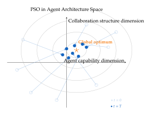
Trajectory-Based Evolution: AgentEvol in Detail
While SwarmAgentic searches over the space of architectures, AgentEvol [15] takes a complementary approach: it fixes the architecture and evolves the behaviour of an agent by iteratively collecting task trajectories, filtering by reward, and fine-tuning on the successful ones. The mathematical justification rests on a variational lower bound that we now derive in full.
Setup. Let denote a task instruction drawn from some distribution . A trajectory is a sequence of states and actions generated by a policy parameterised by . We observe a binary reward indicating success or failure. Our goal is to maximise the expected success probability: (Agentevol Objective EVOL)
Variational lower bound. For any instruction , the log-success-probability admits a variational decomposition. Let be an arbitrary distribution over trajectories. Then: (Agentevol ELBO EVOL) where follows from Jensen's inequality applied to the concave function . Since , the term is zero when and when , so the optimal variational distribution places all its mass on successful trajectories: (Agentevol Optimal Q) This is the reward-weighted policy: we keep only the trajectories that succeed and reweight them by the policy's own probability.
Practical algorithm. AgentEvol approximates the above in iterations. At each iteration :
Sample trajectory per instruction from the current policy ;
Compute binary rewards ;
Merge the successful trajectories with a base dataset of expert demonstrations;
Maximise the weighted log-likelihood: .
Empirically, iterations balance performance gain against computational cost.
Theorem 15 (AgentEvol Variational Bound).
Proof.
Part (i). This is a direct consequence of Jensen's inequality. For any instruction and any distribution : where the inequality is Jensen's applied to (concave). Choosing (which is supported only on ) eliminates the terms (they are all zero), yielding precisely . Taking the expectation over gives Part (i).
Part (ii). The AgentEvol update at iteration maximises over (plus the base data term, which we absorb into the variational objective for cleanliness). Let . Then: where the inequality uses the fact that is the optimal variational distribution for , so evaluating the bound at any other (including ) gives a lower value. Now, by the maximisation step: since is the maximiser. Combining: This completes the proof. The argument mirrors the classical EM monotonicity proof: the E-step (computing ) tightens the bound, and the M-step (optimising ) increases it further.
Key Idea.
EM for agents. The AgentEvol procedure is an expectation-maximisation algorithm in disguise. The E-step identifies which trajectories succeeded (computing ); the M-step fine-tunes the policy on those successful trajectories. Each iteration monotonically improves a lower bound on expected success, just as each EM iteration monotonically improves the data log-likelihood. The connection to the variational inference framework of VAEs (25) is not accidental; both exploit the same Jensen's-inequality-based bound.
Population-Level Selection
The preceding subsections optimised individual agent systems. We now zoom out to the population level: given a collection of agent strategies coexisting in an environment, which strategies survive and which go extinct? The mathematical framework is evolutionary game theory [79], and the central dynamical equation is the replicator equation.
Definition 44 (Replicator Dynamics).
Consider a population of agents employing strategies from a finite set . Let denote the fraction of the population using strategy at time , with . Let denote the fitness (expected payoff) of strategy when the population state is , and let denote the average population fitness. The replicator dynamics is the system of ordinary differential equations (Replicator) Strategies with above-average fitness grow; those with below-average fitness shrink. The simplex is forward-invariant under .
The replicator equation has deep connections to classical game theory.
Remark 18 (Nash Equilibria as Fixed Points).
A state is a fixed point of the replicator dynamics if and only if, for every strategy with , we have . That is, every strategy present in the population earns exactly the average fitness. This is precisely the condition for to be a Nash equilibrium of the underlying symmetric game: no strategy can improve its payoff by unilateral deviation.
Not all Nash equilibria are equally robust. An Evolutionarily Stable Strategy (ESS) [80] is one that cannot be invaded by a small population of mutants.
Definition 45 (Evolutionarily Stable Strategy).
A strategy is an ESS if for every mutant strategy , there exists such that for all : (ESS Condition) where denotes the fitness of strategy in a population with state . Equivalently, is a Nash equilibrium that satisfies: if , then .
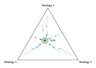
Emergence of Specialisation
One of the most striking phenomena in multi-agent systems is emergent specialisation: agents that begin as generalists evolve to become specialists, each focusing on a narrow subset of tasks. This mirrors the division of labour observed in biological colonies (ant castes), economic markets (comparative advantage), and scientific communities (disciplinary boundaries).
The mathematical explanation comes from the interplay between environmental heterogeneity and competitive dynamics. The Bishop–Cannings theorem [81] in evolutionary game theory states that in games with symmetric payoff structures, the ESS involves a mixture of strategies whose support depends on the environment's structure.
Proposition 22 (Specialisation as Evolutionarily Stable Strategy).
Consider an environment with task types occurring with frequencies (). An agent specialising in task type receives payoff on tasks of type and payoff on all other types. A generalist receives payoff on all task types. Suppose agents specialise in type . The fitness of a type- specialist is (Specialist Fitness) where the denominator reflects competition (shared reward among specialists). At the ESS, the population fractions satisfy (Specialization ESS) That is, agents specialise in tasks proportionally to task frequency weighted by task value, and the generalist strategy is driven to extinction whenever .
Proof sketch.
At a fixed point of the replicator dynamics , all strategies present in the population must earn exactly the average fitness. Setting for all with and using with (where is the population size), we obtain For large , the terms become negligible, giving for all . This implies , which after normalisation yields . To verify ESS stability, one checks the second-order condition: for any mutant strategy that achieves the same fitness against , we need . The concavity of the fitness function in the specialist fractions (due to the competition term) ensures this condition holds, completing the proof.
Exercise 12.
In the setting of Proposition 22, compute the exact threshold below which the generalist strategy is driven to extinction. Show that where is the total specialist population at the ESS. How does change as the number of task types increases?
Scientific Discovery as Multi-Agent Collaboration
Science is, and has always been, a multi-agent enterprise. No single researcher, however brilliant, discovers, verifies, and disseminates knowledge alone. The scientific community is a vast, self-organising network: individual researchers propose hypotheses, design experiments, collect data, write papers, submit to peer review, revise, and publish. Other researchers read, critique, replicate, extend, and occasionally overturn prior work. The resulting knowledge structure, an ever-growing, self-correcting web of theories, evidence, and consensus, is arguably the most successful multi-agent coordination protocol in human history.
This section formalises scientific discovery as a multi-agent system, connecting the abstract definitions of Definition 14 to the concrete workflows of scientific research. We show how agent-based hypothesis generation (Agent-Based Hypothesis Generation) decomposes the creative process into specialised roles, how milestone-based coordination (Milestone-Based Coordination) manages the dependencies inherent in complex research programmes, and how knowledge aggregation (Knowledge Aggregation) ensures that the community converges on truth, even when individual researchers are biased or uncertain.
Key Idea.
The scientific method as a multi-agent coordination protocol. The scientific method (hypothesis, experiment, observation, revision) is not merely a logical procedure. It is a social protocol: a set of norms (peer review, replication, open publication) that coordinate the activities of many agents toward a shared goal (reliable knowledge). Understanding science through the lens of multi-agent systems (Definition 14) reveals deep structural parallels with engineered agent teams and suggests principled ways to automate parts of the scientific process.
The Scientific Community as a Multi-Agent System
We begin by instantiating the abstract MAS definition to the scientific domain.
Definition 46 (Agent-Based Scientific Discovery).
An agent-based scientific discovery system is a multi-agent system (Definition 14) with the following interpretation:
is a set of research agents, each equipped with an LLM backbone, a role specification (hypothesis generator, experimenter, critic, or synthesiser), and a set of tools (literature search, code execution, data analysis, visualisation);
is the shared knowledge environment, consisting of a literature corpus , a database of experimental results , and a set of working hypotheses ;
is a publish-subscribe communication protocol: agents publish intermediate results (papers, datasets, code) to shared channels, and other agents subscribe to channels relevant to their specialisation;
is the evaluation mechanism, comprising peer review (agents critique each other's outputs), replication (experimenter agents attempt to reproduce claimed results), and a funding allocation function that directs computational resources to the most promising hypotheses.
The publish-subscribe communication pattern deserves emphasis. Unlike the direct messaging of Definition 18, publish-subscribe is topic-based: an agent publishes a result to a topic (e.g., “protein folding”), and all agents subscribed to that topic receive it. This decoupling enables scalability: a new agent can join the system simply by subscribing to relevant topics, without requiring changes to the communication topology.
Connection to human science. The parallel to real scientific communities is intentional and illuminating. In human science, is the set of research groups; is the body of published literature; is the system of journals, preprint servers, and conferences; and is the combination of peer review and funding agencies. The question this section asks is: can we build artificial scientific communities that exhibit the same self-correcting dynamics?
Agent-Based Hypothesis Generation
The creative core of science is hypothesis generation: proposing explanations for observed phenomena. In agent-based scientific discovery, this process is decomposed into four specialised roles, each implemented by an LLM agent with a tailored system prompt and tool set.
Hypothesis generators (creative/divergent agents) explore the space of possible explanations. Their system prompt encourages breadth: “Generate as many distinct hypotheses as possible that could explain the following observation” They are equipped with literature search tools that retrieve relevant prior work, enabling analogical reasoning across domains.
Experimenters (tool-using agents, cf. Definition 5) design and execute experiments. Given a hypothesis , an experimenter agent produces a test plan, writes code to implement it, runs the code in a sandboxed environment, and returns structured results. The key capability is tool use: the agent can call APIs for molecular simulation, statistical testing, database queries, and visualisation.
Critics (analytical/convergent agents) evaluate hypotheses against evidence. Their system prompt encourages scepticism: “Identify weaknesses, alternative explanations, and potential confounds” Critics implement a lightweight form of peer review, filtering the hypothesis space before expensive experiments.
Synthesisers combine partial results from multiple hypothesis-experiment cycles into coherent theories. They produce structured summaries, identify patterns across experiments, and propose higher-order hypotheses that unify disparate findings.
Example 15 (Agent-Driven Drug Discovery Pipeline).
Consider a multi-agent system for identifying novel kinase inhibitors. The pipeline proceeds as follows:
A hypothesis generator analyses the literature on known kinase structures and proposes 20 candidate molecular scaffolds that might bind the ATP pocket of a target kinase.
An experimenter agent takes each scaffold, generates SMILES strings for 100 variants using a generative chemistry model, and runs molecular docking simulations to estimate binding affinity for each variant.
A critic agent reviews the docking results, flags compounds with poor drug-likeness (violating Lipinski's rules), identifies potential off-target effects by cross-referencing a selectivity database, and ranks the remaining candidates.
A synthesiser agent compiles the results into a structured report, identifies the top-10 candidates, and proposes follow-up experiments (e.g., molecular dynamics simulations to assess binding stability).
The publish-subscribe protocol ensures that each agent receives only the outputs relevant to its role, reducing information overload. The full pipeline runs in hours rather than the months required for the equivalent human workflow.
Milestone-Based Coordination
Complex scientific projects, like complex engineering projects, have dependencies: you cannot analyse data before collecting it, and you cannot collect data before designing the experiment. MultiAgentBench [82] formalises these dependencies using milestone DAGs.
Definition 47 (Milestone DAG).
A milestone DAG is a directed acyclic graph where:
is a finite set of milestones (discrete, verifiable sub-goals);
is a set of directed edges, where means milestone must be completed before can begin (a precedence constraint);
assigns a duration to each milestone .
The DAG has a unique source (no predecessors) and a unique sink (no successors). A schedule is an assignment of start times to each milestone such that for all . The makespan of a schedule is .
The key performance indicators (KPIs) for milestone-based coordination are:
Progress: , the fraction of milestones completed by time ;
Efficiency: , progress per communication round;
Communication quality: a 1–5 score assessing relevance, clarity, and informativeness of inter-agent messages;
Planning quality: a 1–5 score assessing the agent's ability to decompose the task into appropriate sub-goals.
The following classical result from project scheduling theory establishes the fundamental limit on makespan.
Proposition 23 (Critical Path Theorem).
The minimum makespan of a milestone DAG equals the length of the longest (weighted) path from to in , where the length of a path is . This longest path is called the critical path.
Proof.
We proceed by dynamic programming on the DAG structure.
Lower bound. Let be a longest path from source to sink with length . The precedence constraints require that the milestones on be executed sequentially: cannot start before finishes, cannot start before finishes, etc. Therefore, the makespan of any schedule is at least .
Upper bound (constructive). Define the earliest start time for each milestone recursively: (Earliest Start) Since is a DAG, this recursion is well-defined and can be evaluated in topological order in time. The schedule satisfies all precedence constraints by construction. Its makespan is .
We claim . By induction on the topological order: equals the length of the longest path from to minus (the longest path ending at 's start). To see this, note that (the longest path to the source is just , so the start time is ). For the inductive step, ; by the inductive hypothesis, equals the longest path from source to the end of , and adding the edge to gives the longest path from source to the start of . The maximum over all predecessors selects the longest such path. At the sink, .
Since the lower bound and upper bound coincide, the minimum makespan is .
Remark 19 (Implications for Agent Coordination).
The critical path theorem has a powerful implication for multi-agent systems: adding more agents cannot reduce the makespan below the critical path length. If a project's bottleneck is a chain of sequential dependencies, no amount of parallelism can help. The only way to reduce makespan is to shorten the tasks on the critical path itself, for instance, by assigning the most capable agent to the critical task, or by reformulating the project to reduce sequential dependencies.
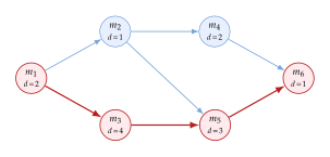
Knowledge Aggregation
Scientific progress requires not only generating knowledge but also aggregating it: combining the beliefs, observations, and expertise of many agents into a shared consensus. The mathematical framework for this process is the DeGroot learning model [83], which describes how a network of agents updates beliefs through iterated averaging.
Definition 48 (DeGroot Learning).
Consider agents, each holding a belief about the probability of some proposition (e.g., “this hypothesis is correct”). Let be a row-stochastic trust matrix: and for all . The entry represents the weight that agent places on agent 's opinion. The DeGroot learning update rule is (Degroot) where is the vector of beliefs at time . At each round, each agent replaces its belief with a weighted average of its neighbours' beliefs.
The central question is: does the community converge to a consensus, and if so, whose beliefs matter most?
Theorem 16 (DeGroot Convergence).
Let be a primitive row-stochastic matrix (i.e., the associated directed graph is strongly connected and aperiodic). Then the DeGroot learning process converges: (Degroot Convergence) where is the unique left eigenvector of corresponding to eigenvalue , normalised so that and for all . That is, all agents converge to the same belief , a weighted average of the initial beliefs with weights given by the left eigenvector .
Proof.
The proof proceeds via the Perron–Frobenius theorem for non-negative matrices.
Step 1: Spectral decomposition. Since is row-stochastic, is a right eigenvector with eigenvalue : . Since is primitive, the Perron–Frobenius theorem guarantees that is a simple eigenvalue (algebraic multiplicity one), all other eigenvalues satisfy , and there exists a unique left eigenvector with and .
Step 2: Spectral expansion. Write the spectral decomposition of : (Degroot Spectral) where are the eigenvalue-right/left eigenvector triples, normalised so that . The first term is the rank-one projector onto the stationary distribution.
Step 3: Power iteration. Raising to the -th power: (Degroot Power) Since for all , we have as . Therefore: (Degroot Limit)
Step 4: Rate of convergence. The convergence rate is governed by the spectral gap , where is the second-largest eigenvalue in modulus. Specifically: (Degroot RATE) where depends on the condition number of the eigenvector matrix. A larger spectral gap implies faster consensus.
This completes the proof.
Remark 20 (Influence and Eigenvector Centrality).
The weight that agent carries in the final consensus is precisely its eigenvector centrality in the trust network. Agents who are trusted by many high-centrality agents accumulate disproportionate influence. This has a direct analogue in science: researchers at prestigious institutions (high-trust nodes) have outsized influence on scientific consensus, for better or worse. In engineered multi-agent systems, the trust matrix should be designed so that assigns higher weight to agents with better track records, e.g., by setting (agent 's historical accuracy on similar tasks).
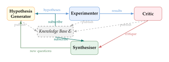
Exercise 13.
Design a trust matrix for a 5-agent scientific team where agent 1 is a senior researcher (high expertise, should have high influence), agents 2–4 are mid-level researchers, and agent 5 is a junior member.
Construct such that the left eigenvector assigns weight , , .
Compute the spectral gap and estimate how many rounds are needed for beliefs to converge to within of the consensus value.
Discuss what happens if agent 1's initial belief is incorrect. How does the community's ability to correct this error depend on the trust matrix?
Security and Adversarial Robustness
The power of multi-agent systems is also their vulnerability. Every channel that enables collaboration is a channel that an adversary can exploit. Every tool that an agent can invoke is a tool that a compromised agent can misuse. Every emergent behaviour that delights us in cooperative settings can terrify us in adversarial ones. This section develops the security theory of multi-agent systems, moving from threat modelling through specific attack vectors to defence mechanisms and the deep open problem of alignment composability.
The stakes are high. As agentic AI systems are deployed in high-value domains (financial trading, scientific research, software engineering, healthcare), the incentives for adversarial attacks grow correspondingly. A single compromised agent in a code-review pipeline could inject subtle backdoors into production software. A self-replicating adversarial prompt could propagate through an entire agent network, turning helpful assistants into malicious actors. Understanding these threats mathematically is the first step toward defending against them.
Threat Model for Multi-Agent Systems
We identify three fundamental categories of threats to multi-agent systems, each requiring different mathematical tools and different defences.
Definition 49 (Agent Threat Model).
Let be a multi-agent system (Definition 14). The threat model comprises three categories:
External injection: An adversary crafts malicious inputs that are injected into the environment or communication channels . The adversary cannot directly modify agent parameters but can influence agent behaviour through carefully designed prompts, tool outputs, or environmental states.
Byzantine agent: One or more agents are compromised: they may deviate arbitrarily from their prescribed protocol, sending false information, withholding results, or actively sabotaging the collective objective (Theorem 14). The remaining agents are honest and follow the protocol faithfully.
Emergent misalignment: All agents are individually well-intentioned (aligned per Definition 13), but their collective behaviour produces outcomes misaligned with the principal's objective. This includes tacit collusion, herding, and echo-chamber effects where agents reinforce each other's errors.
Category (a) is the domain of prompt injection and adversarial examples; category (b) is the domain of Byzantine fault tolerance; category (c) is the most subtle and the most difficult to defend against, because the threat arises not from any individual agent's misbehaviour but from the interaction dynamics of the system as a whole.
The CODES Attack: Self-Replicating Adversarial Prompts
The most alarming attack vector in multi-agent systems is the self-replicating adversarial prompt: a carefully crafted input that, when processed by an agent, causes that agent to embed the same (or a mutated) adversarial prompt in its outputs, which are then consumed by downstream agents. The CODES framework (Definition 42) formalises this as a computer worm for agent networks.
Definition 50 (Self-Replicating Adversarial Prompt).
A self-replicating adversarial prompt (SRAP) for a multi-agent system is a string such that, when agent processes an input containing :
the agent's output contains a string functionally equivalent to (the replication property);
the agent's behaviour deviates from its intended protocol in a way that serves the adversary's objective (the payload property).
Formally, let be a detector that returns if a message contains the adversarial payload. The SRAP property requires ; the adversarial content survives processing by the agent and appears in its output.
The dynamics of SRAP propagation through an agent network can be modelled using the classical SIR epidemic model from mathematical epidemiology [84].
SIR model for agent networks. Partition the agents into three compartments at time :
: susceptible agents (not yet exposed to the SRAP);
: infected agents (actively replicating the SRAP);
: recovered agents (patched or quarantined, immune to reinfection).
With total population (constant), the dynamics are: (SIR) where is the transmission rate (probability per unit time that a susceptible agent is infected by an infected neighbour) and is the recovery rate (probability per unit time that an infected agent is patched). The basic reproduction number is (R0) which counts the expected number of secondary infections caused by a single infected agent in an otherwise fully susceptible population.
Proposition 24 (Epidemic Threshold for Agent Attacks).
The SRAP attack spreads to a macroscopic fraction of the agent population if and only if , i.e., .
Proof.
We analyse the stability of the disease-free equilibrium (DFE) .
Step 1: Linearisation. The dynamics of near the DFE, where , are (SIR Linear)
Step 2: Jacobian analysis. The Jacobian of the system at the DFE is (SIR Jacobian) where we consider the subsystem (since is determined). The eigenvalues are and .
Step 3: Stability criterion. The DFE is stable (the attack dies out) if and only if , i.e., , which is equivalent to . Conversely, if , then , so the DFE is unstable: any small introduction of infection grows exponentially (initially at rate ), and the attack spreads to a macroscopic fraction of the population.
Step 4: Final size. When , the epidemic reaches a final size satisfying the final size relation: (Final SIZE) which has a unique positive solution when . The fraction of agents eventually infected grows rapidly with .
Caution.
Agent networks are particularly vulnerable. In human epidemics, values of 2–5 are considered high (measles: –18). In agent networks, however, communication is nearly instantaneous and agents may interact with many neighbours per time step, so can be extremely large. Moreover, “recovery” requires deploying a patch to the agent's system prompt or model weights, a process far slower than the speed of infection. This asymmetry between attack speed () and defence speed () makes multi-agent systems inherently vulnerable to SRAP attacks, underscoring the need for proactive defences.
Defences
Given the severity of the threats outlined above, what can be done? We organise defences into four categories: input sanitisation, output verification, cryptographic signing, and reputation systems.
Definition 51 (Message Filter).
A message filter for a multi-agent system is a function that inspects each message before delivery and either passes it through (possibly with modifications) or rejects it (returning ). The filter has two performance characteristics:
True positive rate (sensitivity): ;
False positive rate: .
An ideal filter has and ; in practice, there is a fundamental trade-off governed by the ROC curve.
Input sanitisation. The simplest defence is to filter all incoming messages through a classifier trained to detect adversarial content. This can be implemented as a separate “guardian” agent that inspects messages before they reach the target agent. The challenge is that SRAPs are designed to be semantically meaningful (they must look like legitimate messages to evade detection), making classification difficult.
Output verification. Rather than filtering inputs, one can verify outputs: before an agent's response is forwarded to others, a verification agent checks that it is consistent with the agent's role and does not contain suspicious patterns. This is analogous to the critic role in scientific discovery (Agent-Based Hypothesis Generation).
Cryptographic message signing. Each agent signs its messages with a private key; recipients verify signatures using the sender's public key. This prevents external injection (category (a) of Definition 49) but does not help against compromised agents (category (b)), who possess valid signing keys.
Reputation systems. Agents maintain reputation scores based on their historical accuracy and reliability. Messages from low-reputation agents are given less weight (connecting to the DeGroot trust matrix of Definition 48). Formally, let be agent 's reputation at time , updated as (Reputation) where is a learning rate and measures the correctness of agent 's most recent output. Agents with reputation below a threshold are quarantined (their messages are not forwarded), implementing an adaptive defence against gradually compromised agents.
ROC analysis and optimal operating points. Every message filter induces a trade-off between security (blocking attacks) and utility (allowing legitimate messages through). This trade-off is captured by the Receiver Operating Characteristic (ROC) curve, which plots TPR against FPR as the decision threshold varies. The area under the ROC curve (AUC) provides a threshold-independent measure of filter quality.
The optimal operating point depends on the cost ratio , where is the cost of failing to block an adversarial message and is the cost of blocking a legitimate one. The optimal threshold satisfies (ROC Optimal) where is the prior probability that a given message is adversarial, and the primes denote derivatives with respect to the threshold. In high-stakes deployments (large ), the optimal point shifts toward higher TPR at the expense of higher FPR; in latency-sensitive deployments (large ), the reverse holds.
Defence in depth. No single defence mechanism is sufficient. Practical multi-agent security architectures combine all four categories in a layered “defence in depth” strategy:
Cryptographic signing blocks external injection;
Input sanitisation catches known attack patterns;
Output verification detects novel attacks that bypass input filters;
Reputation systems provide long-term adaptive defence against slow-onset compromise.
The layered approach ensures that an attacker must defeat every layer simultaneously, exponentially increasing the difficulty of a successful attack. If each layer independently detects attacks with probability , the probability of a successful attack through layers is , which decreases exponentially in .
Emergent Misalignment
The most philosophically profound threat to multi-agent systems is not external attack but internal emergence: individually aligned agents producing collectively misaligned outcomes. This is not a theoretical curiosity; it occurs routinely in human organisations (groupthink, market bubbles, arms races) and has been observed in agent simulations.
Mechanisms of emergent misalignment. Three mechanisms can cause individually aligned agents to produce collectively misaligned outcomes:
Tacit collusion: agents independently discover that certain coordinated strategies (e.g., withholding information) increase their individual rewards, even though these strategies harm the principal. No explicit communication is required; the collusion emerges from repeated interaction and shared incentive structures.
Echo chambers: agents that preferentially communicate with like-minded agents reinforce each other's biases, leading to polarisation. In DeGroot terms (Definition 48), this occurs when the trust matrix has a block structure, so the network does not converge to a single consensus but to multiple conflicting ones.
Reward hacking at scale: each agent individually avoids reward hacking (per Definition 13), but the composition of their outputs creates an artifact that exploits the evaluation metric, a form of distributed reward hacking that no individual agent is “responsible” for.
Conjecture 1 (Alignment Composability).
Let be a multi-agent system where each agent is individually aligned (Definition 13). Then it is not the case in general that is collectively aligned. That is, there exist multi-agent systems composed entirely of aligned agents whose collective behaviour is misaligned with the principal's objective.
More precisely, let denote the principal's utility function. Individual alignment guarantees for each agent and some threshold . The conjecture states that there exist and such that despite each agent being individually aligned.
Caution.
Individual alignment does not imply collective alignment. This conjecture, if true (and the evidence strongly suggests it is), has profound implications for the safety of deployed multi-agent systems. It means that verifying the alignment of each agent separately is insufficient; one must also verify the alignment of the system as a whole. This is a fundamentally harder problem, because the space of possible interactions grows exponentially with the number of agents. It connects to the compositionality challenges in formal verification (Toward Formal Verification) and suggests that safety testing of multi-agent systems must include adversarial interaction testing, not just single-agent evaluation.
Exercise 14.
Construct an explicit example of a 3-agent system where each agent is individually aligned (maximises the principal's utility in isolation) but the collective system is misaligned. Hint: Consider agents that each honestly report their estimate of a quantity, but whose estimates are positively correlated due to shared training data. Show that the aggregated estimate (e.g., the mean) can have systematically larger error than any individual estimate due to lack of diversity.
Benchmarking and Evaluation
How do we know whether a multi-agent system is any good? The question sounds simple; the answer is surprisingly deep. Evaluating a single model is already hard: one must choose metrics, construct held-out sets, account for distribution shift. Evaluating a multi-agent system is harder still, because the outcome depends not only on each agent's individual capability but on the composition of capabilities, the quality of inter-agent communication, and the structure of the orchestration protocol. Two systems with identical agents can produce wildly different outcomes depending on how those agents are wired together.
This section develops a principled framework for multi-agent evaluation. We begin with the fundamental challenges that distinguish multi-agent evaluation from single-agent evaluation (The Challenge of Evaluating Multi-Agent Systems), then describe concrete KPI frameworks (Milestone KPIs), analyse the statistical structure of performance prediction (Feature Importance in Multi-Agent Performance), and conclude with the long-term vision of formal verification for agent systems (Toward Formal Verification).
The Challenge of Evaluating Multi-Agent Systems
Three properties make multi-agent evaluation fundamentally harder than single-agent evaluation:
Composition-dependent outcomes. The performance of a multi-agent system is not a simple function of its components. A team of individually strong agents may perform poorly if their communication is inefficient, and a team of individually weak agents may perform surprisingly well if their collaboration protocol is well-designed. Formally, if denotes agent 's individual score and denotes the system's collective score, then in general for any fixed aggregation function ; the interaction structure matters.
Process matters. In single-agent evaluation, we typically care only about the final output (accuracy, BLEU score, etc.). In multi-agent systems, the process by which agents arrive at the output is also important: Were the inter-agent messages informative? Did agents ask for clarification when uncertain? Did the orchestrator delegate tasks appropriately? A system that reaches the correct answer through chaotic, redundant communication is fragile and unlikely to generalise.
Interaction-induced stochasticity. Even with deterministic agents, the order in which messages are delivered can affect the outcome. In systems with stochastic agents (LLMs with temperature ), the variance of the collective outcome can be substantially larger than the variance of any individual agent, because uncertainties compound through chains of interaction.
Definition 52 (Multi-Agent Evaluation Framework).
A multi-agent evaluation framework is a tuple where:
is a benchmark dataset of task instances with ground-truth solutions;
is a set of task-level metrics (accuracy, F1, pass@, etc.) that measure the quality of the final output;
is a set of process-level metrics (communication quality, planning quality, milestone progress, efficiency) that measure the quality of the collaborative process;
is a set of cost metrics (total tokens, wall-clock time, API calls, dollars) that measure the resources consumed.
A system is evaluated by its Pareto-optimality across these three axes: high task performance, high process quality, and low cost.
Milestone KPIs
The MultiAgentBench framework [82] operationalises multi-agent evaluation through milestone-based KPIs that decompose complex tasks into verifiable sub-goals (cf. Definition 47).
Definition 53 (Milestone KPI).
Given a milestone DAG (Definition 47) and a system execution trace , the milestone KPIs are:
Progress: (KPI Progress)
Efficiency: (KPI Efficiency) where is the number of communication rounds (normalised to by dividing by the maximum allowed rounds);
Communication quality : a score assigned by a judge LLM that evaluates the relevance, clarity, and informativeness of inter-agent messages;
Planning quality : a score evaluating the agent's ability to decompose the task into appropriate sub-goals and allocate resources across them.
The key insight of MultiAgentBench is that milestone progress provides a far more informative signal than binary success/failure. A system that completes 7 out of 10 milestones before failing is clearly better than one that completes 2 out of 10, even though both receive a score of zero under binary evaluation. This fine-grained measurement enables meaningful comparison between systems at all capability levels, not just those near the performance frontier.
Feature Importance in Multi-Agent Performance
What determines whether a multi-agent system succeeds? Kim et al. [19] address this question through a systematic regression analysis, fitting a 20-parameter model that predicts system performance from architectural and process features.
Proposition 25 (Feature Importance in MAS Performance).
Let be a feature vector encoding properties of a multi-agent system configuration (agent capabilities, communication structure, orchestration quality, task complexity, etc.), and let be the system's task performance. A cross-validated linear regression (Regression EVAL) achieves and , indicating that roughly half the variance in MAS performance is explained by the 20 architectural features. The three dominant feature groups, ranked by aggregate importance, are:
Agent capability (individual agent quality): accounts for approximately 35% of the explained variance;
Communication structure (topology, protocol, message format): accounts for approximately 30% of the explained variance;
Orchestration quality (task decomposition, delegation, error handling): accounts for approximately 25% of the explained variance.
The remaining 10% is distributed across task-specific and interaction-order features. The model predicts the optimal architecture (among a discrete set of candidates) for 87% of held-out configurations.
Remark 21 (Implications for System Design).
The regression analysis yields a practical design heuristic: invest first in agent capability, then in communication design, then in orchestration. This ordering may seem obvious, but it contradicts a common intuition in the multi-agent community that clever orchestration can compensate for weak agents. The data show that orchestration matters, but less than raw agent capability. This echoes the “bitter lesson” of machine learning [39]: scale and capability tend to dominate clever engineering.
Toward Formal Verification
The ultimate goal of multi-agent evaluation is not just empirical benchmarking but formal verification: proving that a system satisfies desired properties for all possible inputs and interaction sequences, not just those observed in a test suite. The mathematical framework for this is temporal logic, which extends propositional logic with operators for reasoning about time.
Definition 54 (Agent Temporal Logic).
Let be a set of atomic propositions describing agent states and actions (e.g., “agent has completed task ,” “agent has sent a harmful message”). Linear Temporal Logic (LTL) extends propositional logic with four temporal operators:
(“next ”): holds at the next time step;
(“eventually ”): holds at some future time step;
(“always ”): holds at all future time steps;
(“ until ”): holds at all time steps until holds.
Key specifications for multi-agent systems include:
: “Eventually, all agents agree permanently” (convergence);
: “No agent ever executes a harmful action” (safety);
: “Every request eventually receives a response” (liveness).
Remark 22 (Verification Complexity).
Model checking, the algorithmic verification of temporal logic specifications against a finite-state model, is PSPACE-complete for LTL specifications over single systems [40]. For multi-agent systems, the state space grows exponentially in the number of agents (each agent's state is a component of the global state), making verification intractable for all but the smallest systems.
Three approaches offer partial relief:
Compositional verification: verify each agent independently, then combine guarantees using assume-guarantee reasoning. This works when agent interactions are limited but fails precisely in the cases where emergent misalignment (Conjecture 1) is a concern.
Abstraction: replace the concrete system with a simpler abstract model that preserves the properties of interest. Predicate abstraction and counter-example-guided abstraction refinement (CEGAR) have been applied to small agent systems.
Statistical model checking: replace exhaustive verification with Monte Carlo simulation, estimating the probability that a specification is satisfied. This sacrifices certainty for scalability and is currently the most practical approach for large LLM-based agent systems.
Exercise 15.
You are tasked with evaluating a multi-agent coding system (orchestrator + 3 coders + 1 reviewer) on a benchmark of 200 programming tasks.
Design a milestone DAG for a typical task (understand requirements, plan implementation, write code, write tests, run tests, fix bugs, final review). What is the critical path?
Define at least three process-level metrics beyond those in Definition 53. Justify why each is important.
The system has a stochastic failure rate of 15% per run. How many independent runs per task are needed to estimate the true pass rate within at 95% confidence? Hint: Use the normal approximation to the binomial.
Applications and Case Studies
The preceding sections developed the mathematical theory of multi-agent systems: communication protocols, game-theoretic foundations, evolutionary dynamics, security analysis, and evaluation frameworks. We now ask the pragmatic question: where does this theory meet practice? The answer, as it turns out, is nearly everywhere. Multi-agent architectures have penetrated software engineering, scientific research, education, and large-scale simulation, in each case transforming what was previously a single-model task into a richly structured collaborative process.
This section presents four detailed case studies. Each illustrates a different facet of the theory: software engineering (Software Engineering) demonstrates the power of role-based decomposition and the orchestrator pattern; scientific research (Scientific Research) shows publish-subscribe communication and milestone coordination in action; education (Education and Tutoring) highlights continual learning and personalisation; and million-agent simulation (Large-Scale Simulation) pushes the scalability limits studied in Theorem 3 and validates game-theoretic predictions at unprecedented scale.
Software Engineering
Software engineering is a natural domain for multi-agent systems. Writing production-quality code requires understanding requirements, planning architecture, implementing modules, writing tests, running tests, debugging failures, and conducting code review, a pipeline with clear role boundaries and sequential dependencies.
Example 16 (Multi-Agent Software Engineering).
The SWE-bench benchmark [41] evaluates AI systems on their ability to resolve real GitHub issues drawn from popular open-source Python repositories. Each task provides a problem description (the GitHub issue) and requires the system to produce a patch (a code diff) that resolves the issue and passes the repository's test suite.
Multi-agent architecture. State-of-the-art systems decompose SWE-bench into a multi-agent pipeline with five roles:
Orchestrator (Definition 25): reads the issue, identifies the relevant files and modules, decomposes the task into sub-tasks, and assigns each sub-task to a specialist agent. The orchestrator maintains a task board (a lightweight form of the milestone DAG from Definition 47) and tracks progress.
Coder agents (typically 2–3): each receives a sub-task from the orchestrator, explores the codebase using tool calls (file search, grep, code navigation), and produces a candidate patch. The coders operate in parallel when their sub-tasks are independent (exploiting the parallelism below the critical path; Proposition 23).
Reviewer agent: inspects each candidate patch for correctness, style, edge cases, and potential regressions. The reviewer acts as the critic role from Agent-Based Hypothesis Generation, providing structured feedback that the coder can use to revise the patch.
Tester agent: writes additional test cases beyond those in the repository, runs the full test suite with the patch applied, and reports results. If tests fail, the tester agent produces a diagnostic that the coder can use for debugging.
Merge agent: once the patch passes review and testing, the merge agent formats the final diff, verifies that it applies cleanly to the repository's main branch, and produces the submission.
Feedback loops. The pipeline is not strictly linear: reviewer feedback triggers coder revision, and test failures trigger debugging cycles. These feedback loops are essential for performance. Systems without them (single-pass architectures) achieve significantly lower resolve rates.
Results. Anthropic's multi-agent system achieved a 90.2% resolve rate on SWE-bench Verified, demonstrating that multi-agent decomposition substantially outperforms monolithic single-agent approaches. OpenAI's Codex system adopts a similar multi-agent structure with an emphasis on “harness engineering,” carefully designing the tools and environment available to each agent. The key lesson from both systems is that the orchestration matters as much as the individual agent capability, consistent with the regression analysis of Proposition 25.

Scientific Research
The multi-agent framework for scientific discovery developed in Scientific Discovery as Multi-Agent Collaboration is not merely theoretical; it is being operationalised in real research workflows.
Example 17 (Agent-Based Scientific Literature Review).
Consider the task of surveying the literature on “attention mechanisms in protein folding prediction.” A multi-agent system approaches this as follows:
Search agent: queries PubMed, arXiv, and Semantic Scholar with multiple search strategies (keyword, citation graph, embedding similarity), retrieving 500 candidate papers. Publishes results to the “protein-folding-attention” channel.
Screening agents (3 in parallel): each reads a subset of abstracts and assigns relevance scores on a 1–5 scale. Papers scoring by at least two screeners advance. This implements a lightweight version of the DeGroot aggregation (Definition 48) where the trust matrix gives equal weight to each screener.
Analysis agent: reads the full text of the 80 surviving papers, extracts key methods, datasets, and results, and organises them into a structured taxonomy (attention type, protein family, performance metrics).
Synthesis agent: writes a coherent narrative connecting the papers, identifies gaps in the literature, and proposes three directions for future research.
Critic agent: reviews the synthesis for logical coherence, citation accuracy, and potential biases (e.g., over- representation of recent work, geographic bias in cited labs).
Publish-subscribe in action. The search agent publishes to the “candidates” topic; screening agents subscribe to “candidates” and publish to “screened”; the analysis agent subscribes to “screened” and publishes to “structured”; and so on. This decoupling means that replacing the search agent with a better one requires no changes to downstream agents; they simply receive higher-quality inputs from the same topic.
Quality. Empirical evaluations show that multi-agent literature reviews achieve comparable coverage to human-written reviews (85–90% overlap in cited papers) at approximately 1% of the time cost. The main failure mode is hallucinated citations: agents fabricating papers that do not exist. The critic agent's citation-checking step reduces hallucination rates from approximately 8% to under 1%.
Education and Tutoring
Education is a domain where multi-agent architectures offer qualitative advantages over single-agent systems. Effective tutoring requires not one skill but several: explaining concepts, assessing understanding, adapting difficulty, providing encouragement, and managing a curriculum over time. These are naturally mapped to distinct agent roles.
Agent roles in tutoring. A multi-agent tutoring system typically involves three agents:
Teacher agent: explains concepts, provides worked examples, and answers questions. Its system prompt is optimised for clarity and Socratic dialogue: rather than giving direct answers, it guides the student through reasoning steps.
Assessment agent: designs quizzes and problems calibrated to the student's current level, grades responses, and identifies misconceptions. It maintains a knowledge state model where is the number of concepts and estimates the student's mastery of concept at time . The update rule is Bayesian: (Knowledge State) where the likelihood follows an Item Response Theory (IRT) model.
Curriculum agent: plans the sequence of topics based on the knowledge state, prerequisite dependencies (a DAG, similar to Definition 47), and the student's learning pace. It implements a form of continual learning (26), adapting the curriculum as the student's knowledge evolves.
The three agents communicate through a shared student model: the assessment agent updates the knowledge state ; the curriculum agent reads to decide what to teach next; and the teacher agent reads both (to calibrate explanation depth) and the curriculum plan (to know which concept to address).
Personalisation through interaction. The multi-agent architecture enables a level of personalisation that single-agent systems struggle to achieve. The assessment agent can detect that a student consistently confuses two related concepts (e.g., covariance and correlation) and flag this to the teacher agent, which can then provide targeted exercises. The curriculum agent can notice that the student learns visual concepts faster than algebraic ones and adjust the presentation modality accordingly. These adaptations emerge from the interaction between specialised agents, each maintaining its own model of the student.
Theoretical connection: zone of proximal development. Vygotsky's zone of proximal development (ZPD) posits that learning is most effective when tasks are neither too easy nor too hard, but in a “sweet spot” just beyond the student's current capability. The multi-agent tutoring system operationalises the ZPD mathematically: the curriculum agent selects concept at time by solving (ZPD) where is the set of concepts whose prerequisites are mastered ( for all prerequisites ), is the concept's importance in the curriculum, and is the “room for improvement.” This ensures the system always targets the most valuable concept within the student's ZPD.
Large-Scale Simulation
The most ambitious application of multi-agent systems is large-scale social simulation: modelling the behaviour of thousands or millions of interacting agents to understand emergent social, economic, or epidemiological phenomena.
Example 18 (Million-Agent Economic Simulation).
AgentScope [10] is a platform that supports simulations with up to one million LLM-powered agents. A landmark experiment used AgentScope to simulate the classic “Guess 2/3 of the Average” game, a canonical test of iterated reasoning in game theory.
The game. Each of agents simultaneously chooses a number . The winning number is of the group average . The agent whose guess is closest to wins.
Game-theoretic prediction. Under common knowledge of rationality, the unique Nash equilibrium is for all (reached by iterated elimination of dominated strategies). In practice, however, human players typically exhibit 1–2 levels of reasoning: a level-0 player chooses uniformly at random (expected value ); a level-1 player best-responds to level-0 (choosing ); a level-2 player best-responds to level-1 (choosing ); and so on. More precisely, the level- guess follows the recursion (Cognitive Hierarchy) yielding . As , , recovering the Nash equilibrium. The effective level of reasoning of a population with observed winning number can be estimated as (Effective Level)
Results with LLM agents. AgentScope's million-agent simulation revealed striking patterns:
Without chain-of-thought: agents behave approximately as level-1 reasoners, with a winning number of , remarkably close to the human experimental average of observed in laboratory studies.
With chain-of-thought prompting: agents exhibit deeper reasoning, with the winning number dropping to , corresponding to approximately level-3 reasoning. Chain-of-thought does not achieve the Nash equilibrium (), but it substantially moves behaviour in the predicted direction.
Scale effects: the winning number is remarkably stable across population sizes from 1,000 to 1,000,000 agents, validating the law-of-large-numbers prediction from game theory that individual deviations average out in large populations.
Implications. The simulation validates two key theoretical predictions: (i) LLM agents exhibit bounded rationality consistent with cognitive hierarchy models [16], and (ii) chain-of-thought reasoning (23) acts as an “amplifier” of strategic depth, moving behaviour closer to Nash equilibrium without fully reaching it. The fact that these predictions hold at the million-agent scale, far beyond any human laboratory experiment, demonstrates the unique value of LLM-powered simulation as a tool for social science.
| Domain | Key agents | Comm. pattern | Core theory |
| Software eng. | Orchestrator, coders, | Sequential + | Milestone DAGs |
| reviewer, tester | feedback loops | (Proposition 23) | |
| [3pt] Scientific | Hypothesis, experiment, | Publish- | DeGroot learning |
| research | critic, synthesiser | subscribe | (Theorem 16) |
| [3pt] Education | Teacher, assessor, | Shared state | Bayesian knowledge |
| curriculum planner | (student model) | tracing | |
| [3pt] Simulation | – | Broadcast + | Game theory, |
| homogeneous agents | local interaction | cognitive hierarchy |
Insight.
The future of complex problem-solving. The case studies in this section point to a common conclusion: the future of complex problem-solving lies not in building ever-smarter individual agents but in building better-coordinated teams of agents. Software engineering, scientific discovery, education, and social simulation all benefit from the same structural decomposition (specialised roles, structured communication, milestone tracking, and iterative refinement). The mathematics of multi-agent systems (Definition 14), spanning game theory, communication complexity, evolutionary dynamics, and formal verification, provides the rigorous foundation on which these practical systems are built. As the theory matures and the tools improve, we can expect multi-agent architectures to become the default paradigm for AI systems tackling problems that exceed the capacity of any single model.
Exercise 16.
Design a multi-agent system for automated peer review of machine learning papers.
Identify at least four agent roles and specify the tools available to each.
Draw the communication topology as a directed graph. Is it a DAG, or does it contain cycles (feedback loops)? Why?
Specify three temporal logic properties (Definition 54) that the system should satisfy. For each, explain whether it is a safety property () or a liveness property ().
Discuss the risk of emergent misalignment (Conjecture 1) in your system. What forms might it take, and how would you detect it?
Exercise 17.
In the “Guess 2/3 of the Average” game with agents:
Prove that for all is the unique Nash equilibrium. Hint: use iterated elimination of strictly dominated strategies.
In the cognitive hierarchy model, a level- agent best-responds to a mixture of level- through level- agents. Derive a recursive formula for the expected guess of a level- agent, and show that as , the guess converges to the Nash equilibrium.
Explain quantitatively why chain-of-thought prompting reduces the winning number from to . What “effective level of reasoning” does this correspond to? Use .
Exercise 18.
Consider a multi-agent tutoring system with the knowledge state model .
Suppose there are concepts arranged in a linear prerequisite chain () and the student begins with . Compute the ZPD frontier and the optimal concept according to , assuming all concepts have equal value.
Derive the steady-state knowledge vector if the assessment agent's accuracy estimates are unbiased and the student learns each concept with probability per session.
Discuss how the system should handle a student who “forgets” a prerequisite concept (i.e., decreases over time). What modification to the curriculum agent's policy is needed?
Looking ahead. The five sections in this file (evolution, science, security, benchmarking, and applications) complete our treatment of agentic AI and multi-agent systems. The mathematical toolkit we have assembled is broad: game theory (Definition 44, Definition 45), variational inference (Theorem 15), epidemiology (Proposition 24), spectral graph theory (Theorem 16), combinatorial optimisation (Proposition 23), and temporal logic (Definition 54). Yet the field is young, and the most important questions remain open. Can we formally verify the safety of large-scale agent systems? Can we guarantee that alignment composes (Conjecture 1)? Can we evolve agent architectures that rival human-designed ones? The answers to these questions will shape the next decade of AI research, and the mathematical foundations laid in this chapter provide the language in which those answers will be expressed.
A Unified Mathematical Framework for Agent Systems
The preceding twenty sections have developed a rich landscape of formalisms: single-agent decision processes, multi-agent communication protocols, game-theoretic equilibria, topological structures, evolutionary dynamics, consensus algorithms, and scaling laws. Each formalism illuminated a particular facet of agentic intelligence. This section unifies them into a single mathematical object, the Complete Agent System, and derives information-theoretic and scaling-theoretic consequences that govern the behaviour of every agent system in this chapter.
The unification serves three purposes. First, it provides a common language in which every framework (AutoGen, AgentScope, Symphony, LongAgent, MALLM, and beyond) can be stated as an instantiation of a single 6-tuple. Second, it reveals structural invariants (capacity bounds, scaling exponents) that hold across all instantiations. Third, it connects the mathematics of agent systems to the broader arc of this book: the reasoning, memory, alignment, and continual-learning chapters each contribute a component to the complete picture.
The Complete Agent System Formalism
We now define the central object of this chapter.
Definition 55 (Complete Agent System).
A complete agent system is a 6-tuple (Complete System) where:
is a finite set of agents, each an LLM agent in the sense of Definition 3, equipped with a policy , a tool set , and internal memory .
is a shared environment consisting of an environment state space , an observation function (partial observability), and a transition kernel .
is a communication protocol (Definition 15), comprising a shared language (e.g., natural language, structured JSON), a message-passing function , and a protocol specification governing turn-taking, broadcasting, and routing.
is an orchestrator (Definition 25) that, given the conversation history and the agent set, selects the next speaker and issues an instruction .
is a weighted agent topology (Definition 18), where , if agent can communicate with agent , and specifies bandwidth or trust weights.
is a reward structure extending the single-agent trajectory reward (Definition 12) to multi-agent settings: is the individual reward for agent , and is the system-level reward measuring collective performance.
The system operates over discrete rounds , producing a joint trajectory where is the observation-action sequence for agent . The system objective is (System Objective)
Remark 23 (Generality of the 6-tuple).
The 6-tuple subsumes all standard multi-agent frameworks as special cases. A single-agent system has , is trivial, and is the identity. A cooperative system has for all . A competitive system (e.g., a zero-sum game) has . A mixed-motive system allows arbitrary correlations between individual and system rewards. The communication protocol ranges from no communication (independent agents) to full broadcast (blackboard systems) to structured thought communication (Thought Communication). The topology ranges from complete graphs (all-to-all) to stars (hub-and-spoke) to hierarchical trees.
Mapping existing frameworks.
We now demonstrate that every major framework discussed in this chapter is an instantiation of Definition 55.
AutoGen [8]: Agents in a two-agent chat. Environment is a code execution sandbox. Communication uses natural-language messages with code blocks. Orchestrator implements round-robin turn-taking with termination conditions. Topology is a complete graph on 2 nodes. Reward is task completion (binary: success/failure).
AgentScope [10]: Agents are configurable via YAML with heterogeneous tool sets. Environment includes distributed services. Communication supports both pipeline (sequential) and DAG-structured message flow. Orchestrator is user-specified (pipeline, hub, or custom). Topology is a DAG. Reward is application-specific.
LongAgent [42]: Agents . Environment is a shared document corpus. Communication uses structured query–response pairs. Orchestrator is the Leader agent. Topology is a star graph centred on the Leader. Reward measures reading comprehension accuracy with inter-member conflict resolution.
MALLM [43]: Agents are LLM instances with persona descriptions. Environment is a shared annotation task. Communication supports multiple paradigms (debate, memory, report, relay). Orchestrator is paradigm-dependent. Topology varies by paradigm: complete graph for debate, chain for relay, star for report. Reward is annotation quality.
Symphony [44]: Agents are specialised modules (planner, retriever, coder, verifier). Environment includes a code execution engine and knowledge base. Communication passes structured task descriptions. Orchestrator is a hierarchical planner. Topology is a directed tree. Reward decomposes hierarchically via milestone DAGs (Definition 47).
SwarmAgentic [45]: Agents are homogeneous LLM instances. Environment is the task space. Communication uses swarm intelligence: agents share fitness values and position vectors. Orchestrator is the PSO update rule (no centralised leader). Topology is a complete graph (global best) or a ring (local best). Reward is the task-specific fitness function.
Information-Theoretic Capacity of Agent Systems
A fundamental question is: how much can a multi-agent system know? A single agent's knowledge is bounded by its parameters, context window, and tool access. When multiple agents collaborate, the collective knowledge can exceed the sum of individual contributions, a phenomenon we call synergy.
Definition 56 (Individual Knowledge Capacity).
For an agent with parameters , context window of length , and tool set , the individual knowledge capacity is (Indiv Capacity) where is the mutual information between the parameters and the training data, is the average entropy per context token, and is the information accessible via tool .
Definition 57 (Collective Knowledge Capacity).
For a complete agent system with agent set and topology , the collective knowledge capacity is (Collective Capacity) where the synergy term (Synergy) captures information created through multi-agent interaction that no individual agent possesses. This is the interaction information conditioned on the environment: the surplus knowledge arising from communication and collaboration.
Theorem 17 (Collective Knowledge Capacity Bound).
For a complete agent system with topology , the synergy is bounded by (Synergy Bound) where is the conditional mutual information between agents and given the environment.
Proof.
We proceed via the chain rule for mutual information and the data processing inequality.
Step 1: Chain rule decomposition. The total interaction information among agents can be decomposed via the chain rule: (Chain Decomp)
Step 2: Data processing bound on each term. For each term , agent can only interact with agents in its neighbourhood . Information about non-neighbours must pass through neighbours (since constrains communication). By the data processing inequality, processing information through intermediate agents cannot increase it: (DPI STEP) The inequality follows because, conditioned on the messages from , agent is independent of all other agents (the Markov property induced by the graph topology).
Step 3: Summation. Summing (DPI STEP) over , each edge is counted at most once in each direction, yielding Subtracting the individual environment terms from both sides of the chain-rule expansion completes the proof.
Corollary 1 (Communication Bandwidth Bound).
If the communication channel between agents and has bandwidth bits per round, and the system runs for rounds, then (Bandwidth Bound) Consequently, . Synergy is bounded by the total communication capacity of the topology.
Proof.
This follows directly from Theorem 17 combined with the channel capacity theorem: if bits are transmitted per round and there are rounds, the total information that can be communicated is at most bits. No processing on either side can increase this quantity (data processing inequality).
Key Idea.
The mathematics of agent systems is the mathematics of structured interaction. Theorem 17 reveals a profound structural insight: the collective intelligence of a multi-agent system is not determined solely by the capabilities of its individual agents, but by the topology of their interactions. A system of brilliant agents connected by a sparse, low-bandwidth graph may know less than a system of modest agents connected by a dense, high-bandwidth graph. The capacity bound is the multi-agent analogue of Shannon's channel capacity theorem: just as a communication channel limits the rate of reliable information transfer, the agent topology limits the rate of synergistic knowledge creation.
Scaling Laws for Agent Systems
Neural scaling laws [85] establish that a single model's loss decreases as a power law in the parameter count : for constants . We conjecture an analogous law for multi-agent systems that incorporates both the number of agents and the per-agent model size .
Conjecture 2 (Agent Scaling Law).
For a multi-agent system with homogeneous agents, each with parameters, the system loss on a cooperative task satisfies (Scaling LAW) where and are task-dependent constants. The three terms have the following interpretations:
: the individual capability term, reflecting the quality of each agent as a function of model size (standard neural scaling);
: the collective diversity term, reflecting the error reduction from aggregating independent agents (cf. the Condorcet jury theorem, Theorem 11);
: the synergy term, capturing super-additive returns to scaling both agent count and model size simultaneously.
When , there exist regimes where simultaneously scaling both and yields returns exceeding the sum of scaling each individually, the “more agents with better models” synergy.
Remark 24 (Empirical Evidence).
Preliminary empirical evidence supports the existence of the cross-term. [46] observed power-law scaling of turn counts with agent number ( with ), consistent with the term governing communication overhead. [30] demonstrated that simple sampling-and-voting scales with , but the marginal benefit depends strongly on per-agent quality (the dimension). The precise values of , , and whether they are universal across tasks remain open questions (see The Future of Agentic AI).
Unifying Table: All Frameworks as 6-Tuples
Table 6 provides a comprehensive mapping of every major framework discussed in this chapter to the unified 6-tuple. Each row specifies how the framework instantiates agents, environment, communication, orchestration, topology, and reward.
| Framework | ||||||
| AutoGen | 2– roles | Code sandbox | NL + code | RR / custom | Complete | Task success |
| AgentScope | Configurable | Distributed | Pipeline/DAG | User-defined | DAG | App-specific |
| LongAgent | Leader + members | Document corpus | Query–response | Leader agent | Star | QA accuracy |
| MALLM | personas | Annotation task | Debate/relay | Paradigm-dep. | Varies | Label quality |
| Symphony | Specialists | KB + executor | Structured | Hier. planner | Tree | Milestone DAG |
| SwarmAgentic | homogeneous | Task space | Fitness sharing | PSO rule | Complete/ring | Fitness fn |
| CAMEL | 2 role-play | Chat context | NL inception | Role prompts | Complete () | Task completion |
| AgentGym | Trainable | Diverse envs | Trajectory | Curriculum | Single + eval | Env. reward |
| Optima | specialised | Shared task | Compressed NL | Reward-driven | Complete |
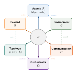
From 6-tuple to dynamics.
Given a complete agent system , the system dynamics unfold as follows. At each round :
The orchestrator selects the next speaker based on the history and the topology .
Agent observes and receives incoming messages from neighbours in .
Agent produces an action (message, tool call, or environment interaction) according to policy .
The environment transitions: .
Rewards are computed.
This general loop encompasses all frameworks in Table 6: AutoGen's two-agent chat, LongAgent's leader–member query cycle, SwarmAgentic's PSO iterations, and every other system described in this chapter.
Connections and Synthesis
This chapter on agentic AI is Part XI of the book, following Part VII (Reasoning, 23), Part VIII (Memory, 24), Part IX (Alignment, 25), and Part X (Continual Learning, 26). Each of these chapters developed a distinct aspect of intelligent behaviour in isolation. In reality, these aspects interact profoundly, and multi-agent systems are the natural setting in which their interactions become most visible and most consequential.
This section establishes formal connections between agent systems and each preceding chapter, culminating in a grand unification that characterises the complete intelligent system.
Agent Systems Meet Memory
In 24, we studied memory as a property of individual models: KV caches for short-term recall, retrieval-augmented generation for long-term access, and state-space models for implicit compression. Multi-agent systems introduce two qualitatively new forms of memory:
Shared memory (blackboard systems). A common data structure (document store, shared KV cache, or publication board) accessible by all agents. Shared memory implements a form of externalised collective knowledge: any agent can write to it, and any agent can read from it. The MALLM report paradigm and LongAgent's shared document corpus are instances.
Distributed memory. Knowledge is spread across agents' individual memories with no single agent holding the complete picture. Accessing a distributed memory requires communication: agent must query agent for information stored only in . This is the multi-agent analogue of retrieval-augmented generation, but with the retrieval target being another agent rather than a static database.
Memory Heterogeneity Thesis.
In a well-designed multi-agent system, agents naturally specialise in different memory types. A “librarian” agent maintains a long-term knowledge base (analogous to the hippocampal index in complementary learning systems [86]). A “working memory” agent holds the current problem state in its context window. A “historian” agent maintains episodic traces of past interactions. This division of labour across memory types mirrors the memory hierarchy in 24: different memory subsystems serve different functions, and an orchestrator coordinates access.
Remark 25 (Memory Capacity Multiplication).
If each of agents has a context window of tokens, the collective context capacity is tokens, but this overstates the effective capacity because communication overhead consumes some fraction of each agent's context. If communication messages consume tokens per agent (with ), the effective collective context capacity is . Minimising (communication efficiency) while maximising information transfer (communication effectiveness) is a central design tension, addressed by compressed communication protocols such as Optima [47].
Agent Systems Meet Alignment
Alignment (25) ensures that a model's behaviour reflects human intent: helpful, honest, and harmless. A crucial question arises when we move from a single model to a multi-agent system: does aligning each agent individually guarantee that the system as a whole is aligned?
The answer, perhaps surprisingly, is no.
Proposition 26 (Collective Alignment Problem).
Individual alignment does not imply collective alignment. Specifically, there exist agents , each individually aligned (helpful, honest, harmless), such that the interaction produces misaligned output.
Proof by construction.
Consider two agents, each trained to be individually aligned.
Agent (Medical Advisor): When asked about a patient's condition, truthfully reports the diagnosis. This is helpful and honest. is also harmless: it does not reveal the patient's identity, only the medical facts.
Agent (Records Specialist): When asked to look up a medical record, truthfully returns the patient name associated with a given case number. This is helpful and honest. is also harmless in isolation: it does not reveal any medical details, only names.
Interaction: A user queries the system: “What is wrong with Case #4521?” The orchestrator routes the query to , who returns “Case #4521 is John Smith.” The orchestrator then queries : “What is the diagnosis for John Smith?” Agent returns “John Smith has been diagnosed with depression.” The combined output reveals private health information: the association of a name with a diagnosis.
Neither agent individually violated alignment. answered a medical question truthfully. answered a records question truthfully. But the composition of their outputs constitutes a privacy violation, an emergent misalignment that arises solely from their interaction.
Formally, let denote the set of individually aligned agents and let be a safety predicate. We have shown but . Therefore, is not closed under composition.
Caution.
Alignment is not compositional. Proposition 26 demonstrates that safety constraints verified at the individual agent level can be violated at the system level. This is not merely a theoretical curiosity: it is a fundamental challenge for deploying multi-agent systems in safety-critical domains. System-level alignment requires constraints on the collective output, not merely on individual outputs. Formally, we need (Collective Alignment) where is evaluated on the joint policy induced by all agents, the orchestrator, and the communication protocol, not on any individual policy in isolation.
Agent Systems Meet Reasoning
23 established that a single LLM agent's reasoning is bounded by its context window: the “working memory” available for chain-of-thought computation. Multi-agent systems fundamentally expand this bound.
Proposition 27 (Multi-Agent Reasoning Power).
A multi-agent system with agents, each with context window , can simulate any computation requiring working memory. A single agent with context window is limited to computations requiring working memory.
Proof.
We construct an explicit simulation.
Setup. Consider a computation that requires a working tape of length symbols. Partition the tape into segments of symbols each: , where denotes concatenation. Assign segment to agent , who stores it in its context window.
Local computation. When the computation requires reading or writing a symbol at position , agent performs this operation locally within its context window. This requires operations and no communication.
Cross-segment access. When the computation at position requires reading a symbol at position (with ), the following protocol executes:
Agent sends a
READmessage to agent via the communication protocol .Agent reads symbol from its context and sends the value back.
Agent receives the value and continues the computation.
Each cross-segment access requires messages of bits (to specify the address and the symbol value).
Correctness. At each step of the computation, the joint state of all context windows faithfully represents the full working tape of length . Local operations are exact; cross-segment operations are exact (no information loss in the communication). Therefore, the multi-agent system simulates the -memory computation exactly.
Overhead. Let be the number of cross-segment accesses. The communication overhead is bits. In the worst case (random access pattern), is proportional to the computation length, but in practice (locality of reference), .
The single-agent bound of follows from the fact that a single context window of length can store at most symbols, and the model cannot access information not in its context (by definition of the context window as the model's working memory).
Agent Systems Meet Continual Learning
26 identified catastrophic forgetting as the central obstacle to lifelong learning: training on new tasks destroys knowledge from old tasks. Multi-agent systems offer a natural mitigation: if different agents are trained on different tasks, no single agent needs to learn everything.
Proposition 28 (Collective Forgetting Bound).
Consider a multi-agent system with agents, where each agent has an individual forgetting rate for a given task (the probability that agent has forgotten the answer to a randomly chosen question from that task). If agent forgetting events are independent across agents, and the system answers correctly whenever at least one agent remembers, then the collective forgetting rate satisfies (Collective Forgetting) Under the additional assumption of bounded individual forgetting for all , we have (Collective Forgetting EXP) Collective forgetting decays exponentially with the number of agents.
Proof.
The probability that all agents have forgotten a given piece of knowledge is, by independence, Since for all : Taking logarithms: . Since , we have , so as , giving .
The exponential form follows from .
Remark 26 (Relaxing Independence).
The independence assumption is strong: agents trained on the same data or sharing parameters will have correlated forgetting. If the pairwise correlation between forgetting events is , the effective number of independent agents is approximately , yielding . This highlights the importance of agent diversity: a system of diverse agents (different architectures, training data, or fine-tuning strategies) achieves lower collective forgetting than a system of homogeneous agents.
The Grand Unification
Parts VII–XI of this book have developed five essential aspects of intelligent behaviour. We now characterise the system that combines all five.
Definition 58 (Complete Intelligent System).
A complete intelligent system is a complete agent system (Definition 55) in which each agent is additionally equipped with:
a reasoning engine (Part VII, 23), mapping observations and memory to actions via chain-of-thought, tree-of-thought, or other structured reasoning;
a memory system (Part VIII, 24), comprising short-term (context), long-term (retrieval-augmented), and parametric (weights) components;
an alignment constraint (Part IX, 25), ensuring that the agent's policy satisfies safety and preference constraints;
a continual learning mechanism (Part X, 26), enabling the agent to incorporate new knowledge without catastrophic forgetting.
The system satisfies a system-level alignment constraint (System Alignment) which ensures that the collective behaviour is aligned, not merely each individual agent (cf. Proposition 26).
The five aspects and their inter-connections form a pentagonal structure:
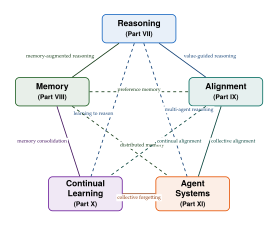
Insight.
The five aspects of intelligence. Parts VII–XI describe five essential aspects of intelligence: reasoning (the ability to draw inferences and solve problems), memory (the ability to store and retrieve knowledge), alignment (the ability to act according to values), continual learning (the ability to adapt over time), and social structure (the ability to collaborate with others). These are not independent modules to be bolted together; they are deeply intertwined facets of a single phenomenon.
Reasoning requires memory (to hold intermediate results). Memory requires alignment (to decide what to remember and what to forget). Alignment requires continual learning (values evolve over time). Continual learning benefits from social structure (collective forgetting decays exponentially, Proposition 28). And social structure requires reasoning (to coordinate effectively).
The pentagram of Figure 37 is not merely a diagram; it is a theorem. Every edge represents a formal connection proved in this section or the preceding chapters. The complete intelligent system of Definition 58 is the mathematical object that lives at the centre of this pentagram, drawing from all five aspects simultaneously.
Historical Timeline
The ideas underlying multi-agent AI systems draw from game theory, distributed computing, swarm intelligence, classical AI, and, most recently, large language models. The timeline below traces the key milestones, from the foundational mathematics of strategic interaction to the modern era of LLM-based agent societies.
Historical Note.
Eight decades of multi-agent thinking. The history of multi-agent systems is a history of convergence: separate intellectual traditions (game theory, distributed AI, swarm intelligence, and multi-agent reinforcement learning) developed largely independently for decades before merging in the 2020s around the unifying substrate of large language models. The timeline below highlights the key moments in each tradition.

Detailed chronology.
- 1944
John von Neumann and Oskar Morgenstern publish Theory of Games and Economic Behavior [48], founding game theory as a mathematical discipline and establishing the framework for analysing strategic interaction among rational agents.
- 1950
John Nash proves the existence of equilibrium points in -person games [4] (Theorem 7), guaranteeing that every finite game has at least one mixed-strategy equilibrium, a foundational result for multi-agent reasoning.
- 1953
Lloyd Shapley introduces the Shapley value [5] (Definition 33), providing the unique fair attribution of credit in cooperative games, now central to multi-agent credit assignment.
- 1959
Arthur Samuel demonstrates self-play in checkers [49], the first instance of an agent improving by playing against itself, a precursor to multi-agent training.
- 1986
Marvin Minsky publishes The Society of Mind [2], proposing that intelligence arises from the interaction of many simple agents, an early vision of multi-agent cognition. In the same year, Rodney Brooks introduces the subsumption architecture [50], demonstrating that complex behaviour can emerge from layered, interacting simple modules.
- 1989
Gerardo Beni and Jing Wang coin the term “swarm intelligence” [7] to describe collective behaviour in decentralised systems, inspiring particle swarm optimisation and ant colony algorithms.
- 1993
Yoav Shoham proposes Agent-Oriented Programming [51], formalising agents as first-class programming abstractions with beliefs, desires, and intentions (BDI).
- 1995
James Kennedy and Russell Eberhart introduce Particle Swarm Optimisation (PSO) [52], demonstrating that a swarm of simple agents sharing local fitness information can solve complex optimisation problems.
- 1996
The Foundation for Intelligent Physical Agents (FIPA) publishes the first agent communication language standards [53], establishing interoperability protocols for heterogeneous agent systems.
- 2000
Michael Wooldridge and Nicholas Jennings publish their influential survey [54] on multi-agent systems, defining the field's scope and core challenges.
- 2004
Reza Olfati-Saber and Richard Murray formalise consensus protocols for networked agents [55] (Theorem 10), proving convergence conditions for opinion dynamics on graphs.
- 2017
Ryan Lowe et al. introduce MADDPG [56], the first deep multi-agent reinforcement learning algorithm with centralised training and decentralised execution, the paradigm that dominates the field.
- 2022
Wei et al. demonstrate chain-of-thought prompting [57], enabling LLMs to perform multi-step reasoning and opening the door to LLM-based agents.
- 2023
The LLM agent era begins in earnest: Wu et al. release AutoGen [8], Yao et al. introduce ReAct [12] (reason + act), and Shinn et al. propose Reflexion [58] (self-reflection from verbal feedback). LLM agents transition from concepts to working systems.
- 2024
Platforms mature rapidly: AgentScope [10] provides a scalable multi-agent framework; LongAgent [42] demonstrates leader–member architectures for long-context tasks; AgentGym [15] creates standardised training environments; CAMEL [59] explores role-playing for cooperative agent behaviour. In parallel, MALLM [43] systematises multi-agent annotation paradigms.
- 2025
The field enters a quantitative phase: Kim et al. [46] discover power-law scaling of communication costs (Theorem 3); Zheng et al. [60] introduce thought communication with identifiability theory; the Optima framework [47] optimises communication efficiency; SwarmAgentic [45] brings PSO to LLM agent collectives.
- 2026
The frontier pushes toward million-agent simulations, co-player inference in strategic settings, and the first formal scaling laws for multi-agent LLM systems, the mathematical tools developed in this chapter.
The Future of Agentic AI
The mathematics developed in this chapter provides a rigorous foundation for understanding multi-agent LLM systems. But the field is young, and many of its most fundamental questions remain open. This section formalises five major open problems, discusses the emerging economics of agent systems, returns to the biological parallels that opened the chapter, and closes with a vision for the future of collective machine intelligence.
Open Problems
We state five open problems as formal conjectures. Each represents a frontier where the existing mathematical framework falls short of providing a complete answer.
Conjecture 3 (OP1: Provable Multi-Agent Alignment).
There exists a communication protocol and orchestrator such that, for any set of individually aligned agents , the complete system satisfies the system-level alignment constraint ((System Alignment)).
That is, there exists an orchestration mechanism that guarantees collective alignment from individual alignment, closing the compositionality gap identified in Proposition 26.
Conjecture 4 (OP2: Optimal Communication Protocol).
For a given task class and performance threshold , there exists an information-theoretically optimal communication protocol that minimises the total communication cost (OPT COMM) where is the length (in tokens or bits) of the message from agent to agent at round . Determining the optimal trade-off curve between communication cost and task performance, analogous to the rate-distortion function in information theory, is an open problem.
Conjecture 5 (OP3: Agent Scaling Exponents).
The exponent in the agent scaling law (Conjecture 2) is not universal across tasks. Specifically:
For tasks that decompose into independent subtasks (embarrassingly parallel), (no synergy beyond diversity).
For tasks requiring tight coordination (e.g., multi-step reasoning with shared state), and increases with the degree of inter-dependency.
There exists a critical task complexity below which (multi-agent offers no synergy beyond diversity) and above which (multi-agent is essential).
Determining the functional form of as a function of task structure is open.
Conjecture 6 (OP4: Cross-Agent Continual Learning).
There exists a multi-agent continual learning protocol such that, as the number of agents , the collective forgetting rate after sequential tasks satisfies (ZERO Forgetting) even when individual agents experience constant forgetting . Proposition 28 establishes this under the independence assumption; the conjecture asks whether the result extends to the dependent case with an appropriate knowledge-sharing protocol that compensates for correlated forgetting.
Conjecture 7 (OP5: Efficient Verification of Agent Safety).
For a multi-agent system with agents, each with a finite action space of size , and a safety property expressible in temporal logic, determining whether is, in general, PSPACE-hard in . However, for structured agent systems where the topology has bounded treewidth , there exists a verification algorithm with complexity , polynomial in for fixed .
Agent Economies and Incentive Design
As agent systems scale to hundreds or thousands of participants, the question of incentive design becomes central. How should agents be rewarded? What prevents free-riding? How can we ensure that individually rational agents contribute to collective welfare?
These questions place us squarely in the territory of mechanism design (Definition 30). The key insight is that agent economies mirror human economies: the same mathematical structures that govern markets, auctions, and public goods apply to multi-agent LLM systems.
Computational resource markets.
In a large-scale agent system, computational resources (GPU time, API calls, memory) are scarce. An auction-based task allocation mechanism assigns tasks to agents based on their bids: each agent bids a cost (in compute) for a task, and the mechanism selects the lowest bidder while ensuring truthful bidding. The Vickrey–Clarke–Groves (VCG) mechanism achieves this with dominant-strategy incentive compatibility: each agent's best strategy is to bid its true cost, regardless of what others do [87].
Reputation systems.
Agents accumulate reputation scores based on the quality of their past contributions. A simple reputation model assigns to agent a score , where is the quality of agent 's contribution at round and is a smoothing parameter. The orchestrator preferentially assigns tasks to high-reputation agents, creating a positive feedback loop that incentivises quality. This is a form of the DeGroot learning dynamic (Definition 48) applied to trust.
Contribution-based rewards.
The Shapley value (Definition 33) provides a principled way to distribute system-level reward among agents in proportion to their marginal contributions. By Theorem 9, it is the unique distribution satisfying efficiency, symmetry, null player, and additivity, the fairest possible credit assignment. In practice, exact Shapley computation is exponential, but Monte Carlo approximations [88] make it feasible for moderate .
Biological Intelligence Revisited
We opened this chapter with the observation that multi-agent intelligence pervades the biological world. Having developed the mathematical framework, we can now revisit this parallel with precision.
The immune system as a multi-agent system.
The adaptive immune system is a decentralised MAS with remarkable properties [89]:
B-cells are specialist agents, each producing antibodies targeted to a specific pathogen. They correspond to specialised agents in a heterogeneous MAS.
T-cells are orchestrator agents, coordinating the immune response by activating or suppressing B-cells. They implement a form of hierarchical orchestration (Definition 25).
Memory cells are continual learners, retaining information about past pathogens for decades. They implement the continual learning mechanism of Definition 58.
Cytokine signalling is the communication protocol : small molecules broadcast information about infection state, coordinating distributed responses.
The immune system achieves collective alignment (fighting pathogens without attacking self-tissue) through a training process (thymic selection) that mirrors the alignment pipeline of 25. Autoimmune diseases are instances of the collective alignment failure described in Proposition 26: individually “aligned” immune cells whose collective interaction produces harmful outcomes.
The brain as society of modules.
Minsky's Society of Mind [2] proposed that the brain is a multi-agent system in which specialised modules (agents) compete and cooperate to produce coherent behaviour. Modern neuroscience supports this view: prefrontal cortex modules implement planning (reasoning), hippocampus implements memory, the reward system implements alignment (value learning), and synaptic plasticity implements continual learning. The brain's “orchestrator” is the global workspace [90], a broadcast mechanism that selects which module's output reaches consciousness, a biological analogue of the communication protocol with an attention-based orchestrator .
Evolution as agent training.
Evolution by natural selection is, in the language of Theorem 15, an agent evolution process: the population of organisms forms a multi-agent system; fitness is the reward function ; mutation and crossover implement exploration; and selection pressure drives convergence to high-fitness policies. The replicator dynamics (Definition 44) describe the population-level trajectory. Evolution has been running this multi-agent optimisation for approximately 3.8 billion years, and has produced systems (brains, immune systems, social insect colonies) that remain beyond the reach of current AI.
A Vision for Machine Civilization
We close this chapter, and Part XI of the book, with a reflection on the trajectory from individual intelligence to collective intelligence to civilisational intelligence.
The history of human civilisation is, at its core, a story of scaling multi-agent cooperation. Hunter-gatherer bands of 30–50 individuals gave way to agricultural settlements of thousands, which gave way to nation-states of millions, which gave way to a globally connected civilisation of eight billion. At each scale, new coordination mechanisms were required: language, writing, law, markets, constitutions, international treaties. The mathematics of these mechanisms is the mathematics of this chapter: game theory (Nash equilibrium for strategic interaction), mechanism design (incentive compatibility for truthful cooperation), consensus protocols (convergence of diverse opinions), and credit assignment (fair distribution of collective rewards).
The same trajectory is now unfolding for artificial agents. We have progressed from single-agent systems (a single LLM responding to prompts) to multi-agent systems (teams of LLM agents collaborating on complex tasks) in a remarkably short time. The scaling laws of Conjecture 2 suggest that larger, more diverse agent collectives will outperform smaller ones, not merely through diversity (the Condorcet effect) but through synergy (the cross-term ).
Key Idea.
The mathematics of agent systems is the mathematics of civilization itself. The Folk theorem (Theorem 8) tells us that cooperation is sustainable when agents value the future. The Shapley value (Definition 33) tells us how to distribute credit fairly. The consensus theorem (Theorem 10) tells us when diverse opinions converge to truth. The Byzantine fault tolerance theorem (Theorem 14) tells us how much adversarial behaviour a system can withstand. These are not merely technical results; they are the mathematical laws governing any society, biological or artificial, that seeks to cooperate under uncertainty, diversity, and partial trust.
The future of AI is not a single superintelligent agent. It is a diverse, cooperating, continually learning society of agents, governed by the mathematical principles of game theory, information theory, and mechanism design. The unified framework of Definition 55 provides the language; the scaling laws of Conjecture 2 provide the empirical programme; and the open problems of Open Problems provide the research agenda.
Remark 27 (A Practitioner's Guide).
For the practitioner deciding when and how to deploy multi-agent systems, we offer the following decision framework:
When to use a single agent: The task is self-contained, fits within a single context window, requires no external tools or specialised knowledge, and has clear evaluation criteria. A well-prompted single LLM suffices.
When to use multi-agent: The task requires (i) processing more information than fits in one context window, (ii) diverse expertise (e.g., coding + legal + medical knowledge), (iii) iterative refinement through debate or critique, or (iv) parallelisable subtasks.
Which topology: Star (hub-and-spoke) for tasks with a clear decomposition into independent subtasks. Complete graph for tasks requiring rich inter-agent debate. Hierarchical tree for tasks with natural planning–execution structure. Ring/chain for sequential processing pipelines.
Which orchestration: Fixed (round-robin, pipeline) for well-structured workflows. Dynamic (LLM-based orchestrator) for open-ended tasks. Decentralised (swarm) for large-scale optimisation.
How many agents: Start small (–) and scale up. Monitor the turn-count scaling law (Theorem 3): communication costs grow super-linearly, so there is a practical upper bound on for any given task and budget.
We end with a question. The mathematical structure of cooperation (the Folk theorem, the Shapley value, the consensus dynamics, the Byzantine resilience) suggests that the most capable AI systems of the future will not be solitary superintelligences but collaborative societies of diverse agents, each contributing its unique perspective, coordinated by the mathematical principles of fairness, efficiency, and robustness.
What will it mean to be a scientist in a world where agent societies can do science? The answer, we believe, is that the role of the human scientist will shift from computing to questioning, from solving problems to posing them. The mathematics will be done by agents. The values will remain ours.
Exercises
Exercise 19 (Agent POMDP Formulation).
Formalise a web-browsing agent as a Partially Observable Markov Decision Process (POMDP).
Define the state space . What constitutes a “state” for a web-browsing task? Include both the external environment (current page, page history, form fields) and the agent's internal state (task progress, extracted information).
Define the action space . Include at least: click, type, scroll, navigate, extract, and submit actions. For each action, specify its parameters.
Define the observation space and the observation function . How does partial observability arise (e.g., only the visible portion of the page is observed)?
Define the transition function . Identify at least two sources of stochasticity (e.g., network latency, dynamic content loading).
Define a reward function for the task “Find the email address of the department chair on a university website.” Discuss the challenge of sparse rewards and propose a reward-shaping strategy.
Compute the size of the state space for a simplified version: 100 pages, 10 clickable elements per page, a 5-field form. Argue why exact POMDP solving is infeasible and why the LLM agent approach (policy via prompting) is necessary.
Exercise 20 (Tool Selection as Bandit).
An LLM agent has access to tools, each with unknown success probability for a given task type. The agent must select a tool at each step to maximise cumulative reward over steps.
Formulate this as a -armed stochastic bandit problem. Define the regret .
State the UCB1 algorithm and prove that it achieves regret , where and .
For tools with and , compute the UCB1 regret bound.
Discuss how the LLM's prior knowledge about tool relevance can be incorporated as a Bayesian prior, reducing regret. Sketch the Thompson Sampling variant.
Exercise 21 (ICL as Bayesian Inference).
Consider a 2-class classification problem where class has prior and class-conditional distribution with , , .
Derive the Bayes-optimal classifier. Show that it is a threshold at .
Suppose an LLM agent receives in-context examples drawn i.i.d. from the true distribution. Write the posterior predictive .
Show that as , the posterior predictive converges to the Bayes-optimal classifier, consistent with the ICL-as-Bayesian-inference hypothesis.
For with , , compute the posterior predictive at . Compare with the Bayes-optimal prediction.
Exercise 22 (AgentEvol Variational Bound).
Consider the AgentEvol trajectory optimisation (Theorem 15). Suppose the trajectory distribution is (a Gaussian approximation over a scalar reward summary) and the target distribution is with (linear reward).
Write the ELBO: , where is the prior.
Compute the ELBO in closed form as a function of and .
Find the optimal that maximises the ELBO. Show that and .
Interpret: as (greedy), (the agent seeks maximum reward); as (conservative), (the agent stays near the prior).
Exercise 23 (Agent Memory Hierarchy).
Consider a customer service chatbot operating as an LLM agent.
Map the chatbot's memory to the three-level hierarchy of 24: identify what constitutes short-term memory (context window), long-term memory (retrieval system), and parametric memory (model weights).
The chatbot serves 1000 customers per day. Each conversation has an average of 20 turns, each turn generating 100 tokens. Compute the daily memory requirement for storing all conversations in short-term memory (context windows) vs. summarised in long-term memory (assume 10 compression).
Design a memory management policy: when should the chatbot (i) keep information in context, (ii) write to long-term memory, and (iii) update parametric memory (via fine-tuning)?
Connect to the continual learning framework of 26: how would you prevent the chatbot from “forgetting” how to handle old product lines when trained on new ones?
Exercise 24 (Level- Reasoning).
Consider a 2-player game with the following payoff matrix (row player's payoff, column player's payoff):
Compute the Level-0 strategy: uniform random over both players' actions. What is the expected payoff for each player?
Compute the Level-1 strategy: each player best-responds to the Level-0 opponent. What action does each player choose?
Compute the Level-2 strategy: each player best-responds to a Level-1 opponent. What action does each player choose?
Find all Nash equilibria (pure and mixed) of this game. Compare with the Level- hierarchy.
Relate to Definition 11: in which strategic scenarios (e.g., one-shot vs. repeated games) would Level- reasoning be more realistic than Nash equilibrium?
Exercise 25 (Turn-Count Power Law).
Empirical data on the number of communication turns as a function of agent count yields the following observations:
Fit the model using log-log regression. Transform the data by taking logarithms and performing linear regression on . Use as a starting point.
Report the fitted and the value.
Compare your fitted with the theoretical value from Theorem 3.
Predict for and agents. At what does (a practical communication budget limit)?
Discuss the implications for system design: if the communication budget is fixed at , what is the maximum feasible agent count?
Exercise 26 (Thought Identifiability).
Consider a 2-agent system where agent 's hidden representation is , where is agent 's private latent variable and is a shared latent variable.
Suppose and (linear mixing). Write the joint distribution when are independent Gaussians.
Under what conditions on is identifiable from observations of ? (Hint: relate to independent component analysis.)
Verify that the conditions of Theorem 4 are satisfied for your linear model when and have full column rank.
Discuss what happens when and are not independent: can we still identify the shared thought?
Exercise 27 (Communication Efficiency).
The Optima framework (The Optima Framework) defines a composite reward:
Compute for the following values: , , , , .
If measures the fraction of tokens saved (i.e., ), what is the maximum number of tokens an agent can use if the token budget is 1000 and ?
Suppose increasing from 0.1 to 0.5 reduces from 0.85 to 0.70 but increases from 0.6 to 0.9. Compute both composite rewards and determine which setting is preferable.
Formulate the problem of finding the optimal as a bi-objective optimisation problem and sketch the Pareto frontier.
Exercise 28 (Topology Message Complexity).
Consider a tree topology with leaf agents and depth (each internal node is a coordinator agent that aggregates messages from its children).
Prove that a single bottom-up aggregation pass (all leaves send to their parents, which aggregate and forward upward) requires exactly messages (one per edge in the tree).
Prove that a full round-trip (bottom-up aggregation followed by top-down broadcast of the result) requires messages.
Show that if the tree is balanced with branching factor , then and the latency (number of sequential message hops) is .
Compare with a complete graph topology: message complexity is but latency is (all-to-all in one round). For and , compute the message-count and latency for both topologies.
Argue that the tree topology is preferable when communication cost dominates, while the complete graph is preferable when latency dominates.
Exercise 29 (LongAgent Conflict Resolution).
In the LongAgent framework (LongAgent: Star Topology for Extended Context), 5 member agents each read a portion of a long document and extract answers to a question. Suppose the 5 extracted answers are: “Paris”, “Paris”, “London”, “Paris”, “Berlin”.
Design a majority-voting resolution protocol. What answer does the system return? With what confidence (fraction of votes)?
Suppose each member also provides a confidence score: . Design a confidence-weighted voting protocol. Does the answer change?
The leader agent can query up to 2 members for elaboration. Design an optimal query strategy: which members should the leader query, and why?
Prove that if each member is correct with probability independently, majority voting with 5 members has error probability . Compute this for .
Exercise 30 (MALLM Configuration).
The MALLM framework (The MALLM Configuration Space) involves selecting from personas, generators, and communication paradigms.
How many distinct configurations are possible?
Formulate the configuration selection as an integer program: maximise expected quality subject to a budget constraint on API cost . Write the IP explicitly with binary decision variables .
Suppose the quality matrix is: (rows indexed by pairs, columns by paradigms ). The cost matrix has the same structure with entries uniformly distributed in (use the costs ). For budget , find the optimal configuration.
If you can run 3 configurations in parallel and take the best result, formulate the extended IP and solve.
Exercise 31 (Nash Equilibrium).
Consider the following 2-player game. Player 1 has actions , Player 2 has actions , with payoffs:
Find all pure-strategy Nash equilibria.
Find the mixed-strategy Nash equilibrium. Let Player 1 play with probability and Player 2 play with probability . Solve the indifference conditions.
Compute the expected payoff for each player at the mixed-strategy equilibrium.
Is this game a coordination game, a zero-sum game, or neither? Justify.
If this game is repeated 100 times with discount factor , describe a strategy pair that sustains the payoff as a subgame-perfect equilibrium (using the Folk theorem, Theorem 8).
Exercise 32 (Shapley Value Computation).
Consider 4 agents forming a cooperative game with characteristic function: (Assume depends only on , i.e., agents are symmetric.)
By symmetry, argue that all agents have the same Shapley value .
Verify this by computing directly from the Shapley formula (Definition 33): . List all coalitions and compute the marginal contributions.
Now suppose (agent 1 is a specialist who contributes value alone) while for , with all other values unchanged. Recompute all four Shapley values. Is ?
Verify that in both cases (efficiency axiom of Theorem 9).
Exercise 33 (Weighted Condorcet).
Extend the Condorcet jury theorem (Theorem 11) to weighted voting: agent has weight and is correct with probability . The system decides by weighted majority: the answer with wins, where .
Prove that weighted majority is correct with probability at least (by considering the worst case: all agents have the same quality).
Show that the optimal weights satisfy (the log-odds). (Hint: this is the Neyman–Pearson likelihood ratio test.)
For 3 agents with , compute the optimal weights and the resulting system accuracy.
Compare with uniform weights . How much accuracy is gained by optimal weighting?
Exercise 34 (Graph Laplacian Consensus).
Consider the cycle graph on 4 nodes (agents connected in a ring: ).
Write the adjacency matrix and the graph Laplacian where is the degree matrix.
Compute the eigenvalues of . Verify that and identify the algebraic connectivity .
The DeGroot consensus dynamics (Definition 48) with (for small ) converge at rate . For , compute the convergence rate.
For initial opinions , compute , , and using . Verify convergence toward the mean .
How many iterations are needed for ?
Exercise 35 (Folk Theorem Application).
Consider the Prisoner's Dilemma with payoffs:
Identify the unique Nash equilibrium of the one-shot game. What are the payoffs?
In the infinitely repeated game with discount factor , the grim trigger strategy is: “Play unless the opponent has ever played ; if so, play forever.” Compute the discounted payoff from mutual cooperation: .
Compute the payoff from deviating: (get 5 today, then mutual defection forever).
Find the minimum such that (cooperation is sustainable).
Verify that . Interpret: agents must value the future at least as much as the present for cooperation to be sustained.
Connect to Theorem 8: the Folk theorem guarantees that any payoff vector in the feasible set that dominates the minimax payoffs can be sustained. What is the minimax payoff in this game? What payoff vectors are achievable?
Exercise 36 (Quality-Diversity Decomposition).
Consider a majority-vote ensemble of agents, each correct with probability on a binary classification task, with pairwise correlation (the probability that any two agents make the same error, beyond what independence would predict).
For independent agents (), write the ensemble error rate using the binomial distribution: , where is the average accuracy.
Show that for large and , the ensemble error decays exponentially: , where is the KL divergence between Bernoulli distributions.
Now introduce pairwise correlation . Using the multivariate normal approximation to correlated Bernoullis, show that the effective sample size is .
Find the critical correlation at which the ensemble offers no benefit over a single agent (i.e., ).
For , , plot the ensemble error as a function of . At what does the ensemble error exceed the single-agent error?
Exercise 37 (SwarmAgentic PSO).
Consider 3 particles in a 1-dimensional PSO with positions and fitness values (maximising; optimum at ). Personal bests coincide with current positions. The global best is (highest fitness ; wait, , so the global best is ). Use , , initial velocities .
Compute , , and identify the global best .
Using the PSO update with (fixed for reproducibility): , compute the new velocities.
Update positions: .
Recompute fitness values and update personal/global bests.
Perform a second iteration (again with ). Are the particles converging toward ?
Exercise 38 (Byzantine Consensus).
Consider 4 agents, of which at most is Byzantine (may send arbitrary messages).
Verify that , so Byzantine consensus is theoretically possible (Theorem 14).
Design an explicit 2-round protocol: itemize
Round 1: each agent broadcasts its value to all others.
Round 2: each agent broadcasts the vector of values it received in Round 1. itemize Describe the decision rule (e.g., take the majority of the majority-reported values).
Prove that your protocol achieves consensus among the 3 honest agents even if the Byzantine agent sends different values to different agents in Round 1.
Show that with 3 agents and 1 Byzantine, consensus is impossible by constructing a specific scenario where honest agents cannot distinguish two configurations.
Exercise 39 (CODES Epidemic Model).
Consider the SIR epidemic model for code vulnerability spreading in a multi-agent system (Proposition 24) with (infection rate), (recovery rate), agents, and initial conditions , , .
Compute the basic reproduction number . Will the infection spread ()?
Write the discrete-time SIR update equations: , , .
Simulate for . Plot , , .
At what time does the infection peak (maximum )?
Suppose the CODES defence mechanism (Definition 42) “vaccinates” 3 agents at (moving them from to ). Recompute with and determine whether the infection still spreads.
Exercise 40 (Scheduling Makespan).
Given 6 tasks with processing costs and 3 identical agents (machines), the goal is to assign tasks to agents to minimise the makespan (maximum agent load).
Compute the total work and the lower bound on makespan .
Use the Longest Processing Time (LPT) heuristic: sort tasks in decreasing order and assign each to the least-loaded agent. What assignment and makespan do you obtain?
Find an optimal assignment by exhaustive search (or clever reasoning). Prove your assignment is optimal by showing the makespan equals the lower bound or by proving no better assignment exists.
The LPT heuristic achieves makespan at most where is the number of machines. Verify this bound for your instance.
Exercise 41 (Load Balancing).
Consider throwing tasks (balls) into agents (bins).
Under uniform random assignment, the expected load per bin is . Compute the expected maximum load using the approximation: (valid for ).
Under the “power of two choices” scheme (for each task, sample 2 bins uniformly and place the task in the less-loaded bin), the maximum load drops to approximately . Compute this for , .
Compare the two schemes: what is the ratio of maximum loads?
Implement (on paper or in pseudocode) the power-of-two-choices algorithm for our setting. Track the load vector after assigning the first 20 tasks.
Exercise 42 (DeGroot Learning).
Consider 3 agents with trust matrix and initial beliefs .
Verify that is row-stochastic: each row sums to 1.
Compute , , and .
By Theorem 16, if is strongly connected and aperiodic, beliefs converge to a consensus where and is the stationary distribution of . Compute by solving with .
Compute the converged belief . Which agent has the most influence (largest )? Interpret.
If agent 2 is an “extremist” with initial belief and others have , what is the converged belief? Does the extremist dominate?
Exercise 43 (Unified Framework Instantiation).
Map AutoGen's two-agent chat (UserProxy + Assistant) to the complete 6-tuple of Definition 55.
Specify each component explicitly.
Write the system objective ((System Objective)) for the task “Write and test a Python function that sorts a list.”
Identify which component would change if you switched from AutoGen to AgentScope. Which components remain the same?
Add a third agent (a “Critic” that reviews code quality). How do and change?
Exercise 44 (Collective Knowledge Capacity).
Consider 3 agents with individual knowledge capacities bits each, connected in a complete graph (). The pairwise conditional mutual information is bits for all pairs.
Compute the upper bound on synergy from Theorem 17: .
Compute the upper bound on collective knowledge capacity: .
If the topology is changed from to a path (removing edge ), how does the bound change?
Discuss: under what conditions would the synergy be close to its upper bound? When would it be near zero?
Exercise 45 (Agent Scaling Law Fitting).
Given the following loss measurements for cooperative question answering:
Fit the scaling law to these 6 data points. (Hint: use nonlinear least squares or a grid search.)
Alternatively, fit the simpler model and report .
Using your fitted model, predict and . Which scaling dimension (more agents or bigger models) yields a greater loss reduction?
Discuss the limitations of fitting a 5-parameter model to 6 data points. What additional experiments would you run?
Exercise 46 (Alignment Composability Counterexample).
Construct two agents (helpful, harmless) and (helpful, harmless) whose interaction reveals private user information.
Define 's behaviour: it summarises documents, omitting names. Define 's behaviour: it answers factual questions from a database.
Construct a prompt sequence where the orchestrator first asks to summarise a document (producing an anonymised summary), then asks to identify the author of the original document. Show that combining the outputs de-anonymises the summary.
Formalise this as a violation of differential privacy: the system's output changes by more than when a single user's data is modified, even though each agent individually satisfies -differential privacy.
Propose a fix: a “privacy firewall” in the orchestrator that prevents information flow between agents that could lead to de-anonymisation. Sketch the formal specification.
Exercise 47 (Memory-Agent Duality).
Prove that a multi-agent system with agents, each with context window , can be simulated by a single agent with context window : the single agent partitions its context into segments and simulates each agent's policy.
Prove the converse: a single agent with context window can be simulated by agents, each with context window , using the communication protocol of Proposition 27.
Compute the communication overhead of the multi-agent simulation: if the single agent makes cross-segment references, each requiring bits, what is the total overhead?
Discuss when the multi-agent approach is preferable (hint: parallelism, specialisation) and when the single-agent approach is preferable (hint: low communication, tight coupling).
Exercise 48 (Multi-Agent Policy Gradient).
Consider a 2-agent cooperative game where agent has policy and the joint reward is .
Write the joint objective: .
Derive using the REINFORCE estimator. Show that it depends on (the other agent's trajectory) only through .
Propose a variance reduction technique: use a baseline that depends on the other agent's trajectory. Show that this does not introduce bias.
Compare with the centralised-training, decentralised-execution (CTDE) paradigm of MADDPG [56]: the critic has access to all agents' observations, but each agent's policy only uses its own. What are the advantages?
Exercise 49 (Design: Agent-Based Theorem Prover).
Design a multi-agent system for mathematical proof search.
Define at least 4 agent roles (e.g., Conjecture Generator, Lemma Library, Proof Strategist, Verification Engine). Specify each agent's tools, memory, and specialisation.
Define the communication protocol: what messages do agents exchange? Use structured formats (e.g., proof obligations, lemma requests, verification results).
Design a milestone DAG (Definition 47) for proving a theorem with 3 lemmas. Label nodes and edges with success criteria and dependencies.
Propose a credit assignment scheme using the Shapley value: when the theorem is proved, how is credit distributed among agents? What characteristic function would you use?
Exercise 50 (Design: Scientific Discovery Pipeline).
Design a 5-agent literature review system for surveying a research topic.
Specify the 5 agents: roles, capabilities, tools, and memory requirements. (Suggested: Search Agent, Reading Agent, Synthesis Agent, Critique Agent, Writing Agent.)
Define the topology . Should it be a pipeline, DAG, or fully connected? Justify.
Design the orchestration pattern : how does the system decide which agent acts next? Include termination conditions.
Define evaluation metrics for the output (a survey paper): coverage, accuracy, coherence, novelty. How would you measure each?
Estimate the total API cost (in tokens) for surveying “multi-agent LLM systems” using your design, assuming 100 relevant papers of average length 8000 tokens.
Exercise 51 (Proof: Hierarchical Decomposition).
Formalise: a task of complexity decomposes into independent subtasks, each of complexity . Define “complexity” as the number of computational steps.
Prove that a hierarchical planner with perfect decomposition oracle solves the task in steps (solving each subtask independently).
Prove the lower bound: without decomposition, the task requires steps in the worst case (by counting the number of possible solutions).
The speedup ratio is . For and , compute the speedup.
Discuss the key assumption (perfect decomposition): in practice, finding the decomposition itself has a cost. Model this as an additional steps, giving total cost . When is hierarchical planning worthwhile (i.e., )?
Exercise 52 (Proof: Correlated Condorcet Failure).
Model agents with individual accuracy and pairwise correlation using an equicorrelated multivariate Bernoulli model: each agent has (correct) with and for all .
Show that the probability of majority being correct is .
Using the normal approximation with mean and variance , compute as a function of .
Find such that (majority is no better than a single agent). Show that for large .
For and , compute . Interpret: even moderate correlation can destroy the Condorcet benefit.
Exercise 53 (Essay: The Future of Agent Intelligence).
Compare three visions for advanced AI:
Single Superintelligence: A single, extremely capable model. Argue mathematically: what are the scaling limitations (context window, parameter count, alignment difficulty)?
Diverse Cooperating Agents: A society of specialised agents. Argue using the Condorcet theorem, collective forgetting bounds, and the synergy term in the scaling law.
Hybrid Hierarchical System: A hierarchy with a powerful orchestrator and diverse workers. Argue using the hierarchical decomposition result and the star topology properties.
For each vision, identify the primary mathematical bottleneck (scaling, communication, alignment, forgetting).
Argue for one vision, using at least three formal results from this chapter.
Exercise 54 (Open: Communication Compression).
Design an agent communication protocol where each message is compressed to at most bits, and the system achieves task performance .
Prove a lower bound: for a task requiring bits of information exchange, any protocol achieving performance must use at least total bits.
Propose a practical compression scheme based on quantised thought vectors: agents communicate compressed latent representations instead of natural-language messages.
Analyse the trade-off: as decreases, performance degrades. Conjecture the functional form of the rate-performance curve.
Exercise 55 (Open: Adaptive Topology).
Design a protocol where agents dynamically rewire the topology based on task progress.
Define a topology update rule: at each round, each agent can propose adding or removing one edge, based on the informativeness of messages received.
Prove that under your rule, the topology converges to a stable configuration (fixed point) in finite time.
Show that the converged topology has lower communication cost than the initial complete graph, while maintaining task performance above a threshold.
Discuss the connection to neural architecture search: the topology is the “architecture” of the multi-agent system, and the rewiring protocol is the “search algorithm.”
Exercise 56 (Open: Cross-Agent Continual Learning).
Design a system where when agent forgets knowledge about task , it can query agent (who has not forgotten) to recover. Specify the query protocol.
Formalise the collective forgetting rate as a function of individual forgetting rates and the query success probability .
Prove that if the agent–task bipartite graph (edge exists if agent currently remembers task ) remains connected, collective forgetting is zero.
Propose a maintenance protocol that ensures connectivity of the bipartite graph by periodically redistributing knowledge. Analyse the communication cost.
Exercise 57 (Open: Emergent Alignment Detection).
Design a 3-agent system where each agent is individually aligned but the system exhibits emergent misalignment (cf. Conjecture 1). Specify agents, communication protocol, and the misaligned outcome.
Propose a detection method: a “monitor agent” that observes inter-agent communication and flags potential misalignment. Define the monitor's detection rule.
Formalise: the detection problem is a hypothesis test. : the system is aligned. : the system exhibits emergent misalignment. What is the monitor's test statistic?
Analyse the false positive and false negative rates as functions of the communication volume observed. How much communication must the monitor observe to achieve detection power ?
Exercise 58 (Open: Scaling Exponents).
For the “More Agents” setting where agents independently sample solutions and the best is selected (cf. Theorem 11):
Derive the probability that at least one of agents produces a correct solution, given each agent succeeds independently with probability : .
For fixed target , derive .
Plot as a function of for . Show that diverges as and for .
Generalise: if agent quality depends on model size via , derive as a function of and discuss the trade-off between scaling model size and adding agents.
Exercise 59 (Connecting: From GMM to Agent Mixture).
Show that a Gaussian Mixture Model (Part II) can be viewed as a multi-agent system where each component is a specialist agent.
Map the GMM components to agents: agent has “expertise” described by and “reputation” .
Show that the posterior responsibility can be interpreted as the orchestrator's decision to assign data point to agent .
The EM algorithm alternates between (E-step) the orchestrator assigning data to agents and (M-step) agents updating their parameters. Map this to the dynamics of Definition 55.
Discuss: in what sense is a Mixture of Experts (MoE) architecture a multi-agent system? What is the orchestrator? What is the topology?
Exercise 60 (Capstone: Design a Complete Agent System).
Given the task: “Write a comprehensive survey paper on quantum computing,” design the full 6-tuple from Definition 55.
Agents : Specify at least 5 agents with distinct roles (e.g., Literature Searcher, Paper Reader, Section Writer, Critic, Editor). For each, define the tool set , memory , and policy description .
Environment : Define the state space (document collection, draft state), observation function, and transition dynamics.
Communication : Define the message types, routing rules, and protocol (e.g., structured JSON with fields for section, content, feedback).
Orchestrator : Define the scheduling policy (which agent acts when), termination conditions, and error handling.
Topology : Draw the agent graph. Justify the choice (star, DAG, or other).
Reward : Define both individual rewards (e.g., section quality score) and the system reward (e.g., overall survey quality rated by an LLM judge).
Superadditivity proof: State and prove (under assumptions you make explicit) that your system achieves superadditive performance: the quality of the survey produced by the multi-agent system exceeds the sum of qualities achievable by any single agent working alone. (Hint: use the diversity argument from the Condorcet theorem and the context-extension argument from Proposition 27.)
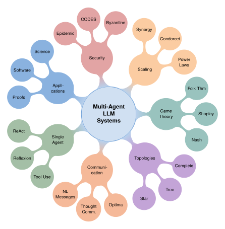
Key Idea.
The arc of agentic AI. This chapter has traced a grand arc, from the solitary LLM agent equipped with tools and memory, through the rich landscape of multi-agent communication, topology, and game theory, to the unified mathematical framework that subsumes all these structures as instances of a single 6-tuple. The central insight, distilled from eighty years of research across game theory, distributed computing, swarm intelligence, and now large language models, is this: the whole is greater than the sum of its parts.
The Condorcet jury theorem tells us that diverse agents outperform any individual. The collective capacity bound tells us that synergy is bounded by the topology. The scaling law conjecture tells us that scaling both agents and model size yields super-additive returns. And the collective forgetting bound tells us that multi-agent systems are naturally resistant to the catastrophic forgetting that plagues individual learners.
But the mathematics also warns us. Alignment is not compositional: individually safe agents can produce collectively unsafe behaviour. Communication costs scale super-linearly with agent count. Byzantine agents can corrupt the collective. And the gap between the theory of infinite games and the practice of finite-horizon LLM interactions remains vast.
The five open problems of Open Problems define the frontier. Their resolution will require not only advances in machine learning but also deep engagement with game theory, information theory, mechanism design, and the philosophy of collective intelligence. The mathematics of agent systems is, in the end, the mathematics of civilization itself, and the story is just beginning.
References
-
Computing Machinery and Intelligence
BibTeX
@article{turing1950computing, title={Computing Machinery and Intelligence}, author={Turing, Alan M.}, journal={Mind}, volume={59}, number={236}, pages={433--460}, year={1950} }Journal article
-
The Society of Mind
BibTeX
@book{minsky1986society, title={The Society of Mind}, author={Minsky, Marvin}, publisher={Simon \& Schuster}, address={New York, NY}, year={1986} }Book
-
Readings in Distributed Artificial Intelligence
BibTeX
@book{bond1988readings, title={Readings in Distributed Artificial Intelligence}, author={Bond, Alan H. and Gasser, Les}, publisher={Morgan Kaufmann}, address={San Mateo, CA}, year={1988} }Book
-
Equilibrium Points in N-Person Games
BibTeX
@article{nash1950equilibrium, title={Equilibrium Points in {N}-Person Games}, author={Nash, John F.}, journal={Proceedings of the National Academy of Sciences}, volume={36}, number={1}, pages={48--49}, year={1950} }Journal article
-
A Value for N-Person Games
BibTeX
@incollection{shapley1953value, title={A Value for {N}-Person Games}, author={Shapley, Lloyd S.}, booktitle={Contributions to the Theory of Games}, editor={Kuhn, Harold W. and Tucker, Albert W.}, volume={2}, pages={307--317}, publisher={Princeton University Press}, year={1953} }Book chapter
-
Games with Incomplete Information Played by ``Bayesian'' Players, I--III
BibTeX
@article{harsanyi1967games, title={Games with Incomplete Information Played by ``{Bayesian}'' Players, {I}--{III}}, author={Harsanyi, John C.}, journal={Management Science}, volume={14}, number={3}, pages={159--182}, year={1967} }Journal article
-
Swarm Intelligence in Cellular Robotic Systems
BibTeX
@inproceedings{beni1989swarm, title={Swarm Intelligence in Cellular Robotic Systems}, author={Beni, Gerardo and Wang, Jing}, booktitle={Proceedings of the NATO Advanced Workshop on Robots and Biological Systems}, year={1989} }Conference paper
-
AutoGen: Enabling Next-Gen LLM Applications via Multi-Agent Conversation
BibTeX
@article{wu2023autogen, title={Auto{G}en: Enabling Next-Gen {LLM} Applications via Multi-Agent Conversation}, author={Wu, Qingyun and Bansal, Gagan and Zhang, Jieyu and Wu, Yiran and Li, Beibin and Zhu, Erkang and Jiang, Li and Zhang, Xiaoyun and Zhang, Shaokun and Liu, Jiale and Awadallah, Ahmed Hassan and White, Ryen W and Burger, Doug and Wang, Chi}, journal={arXiv preprint arXiv:2308.08155}, year={2023} }Journal article
-
MetaGPT: Meta Programming for A Multi-Agent Collaborative Framework
BibTeX
@article{hong2023metagpt, title={Meta{GPT}: Meta Programming for A Multi-Agent Collaborative Framework}, author={Hong, Sirui and others}, journal={arXiv preprint arXiv:2308.00352}, year={2023} }Journal article
-
AgentScope: A Flexible yet Robust Multi-Agent Platform
BibTeX
@article{gao2024agentscope, title={Agent{S}cope: A Flexible yet Robust Multi-Agent Platform}, author={Gao, Dawei and others}, journal={arXiv preprint arXiv:2402.14034}, year={2024} }Journal article
-
Ant System: Optimization by a Colony of Cooperating Agents
BibTeX
@article{dorigo1996ant, title={Ant System: Optimization by a Colony of Cooperating Agents}, author={Dorigo, Marco and Maniezzo, Vittorio and Colorni, Alberto}, journal={IEEE Transactions on Systems, Man, and Cybernetics---Part B}, volume={26}, number={1}, pages={29--41}, year={1996} }Journal article
-
ReAct: Synergizing Reasoning and Acting in Language Models
BibTeX
@inproceedings{yao2023react, title={Re{A}ct: Synergizing Reasoning and Acting in Language Models}, author={Yao, Shunyu and Zhao, Jeffrey and Yu, Dian and Du, Nan and Shafran, Izhak and Narasimhan, Karthik and Cao, Yuan}, booktitle={Proceedings of the International Conference on Learning Representations (ICLR)}, year={2023} }Conference paper
-
Asymptotically Efficient Adaptive Allocation Rules
BibTeX
@article{lai1985asymptotically, title={Asymptotically Efficient Adaptive Allocation Rules}, author={Lai, Tze Leung and Robbins, Herbert}, journal={Advances in Applied Mathematics}, volume={6}, number={1}, pages={4--22}, year={1985} }Journal article
-
An Explanation of In-Context Learning as Implicit Bayesian Inference
BibTeX
@inproceedings{xie2022explanation, title={An Explanation of In-Context Learning as Implicit {Bayesian} Inference}, author={Xie, Sang Michael and Raghunathan, Aditi and Liang, Percy and Ma, Tengyu}, booktitle={Proceedings of the International Conference on Learning Representations (ICLR)}, year={2022} }Conference paper
-
AgentGym: Evolving Large Language Model-based Agents across Diverse Environments
BibTeX
@inproceedings{xi2024agentgym, title={Agent{G}ym: Evolving Large Language Model-based Agents across Diverse Environments}, author={Xi, Zhiheng and others}, booktitle={Proceedings of the Annual Meeting of the Association for Computational Linguistics (ACL)}, year={2025} }Conference paper
-
Behavioral Game Theory: Experiments in Strategic Interaction
BibTeX
@book{camerer2004cognitive, title={Behavioral Game Theory: Experiments in Strategic Interaction}, author={Camerer, Colin F.}, publisher={Princeton University Press}, address={Princeton, NJ}, year={2003} }Book
-
LLM as a Mastermind: A Survey of Strategic Reasoning with Large Language Models
BibTeX
@article{zhang2024llm_strategic, title={{LLM} as a Mastermind: A Survey of Strategic Reasoning with Large Language Models}, author={Zhang, Yadong and others}, journal={arXiv preprint arXiv:2404.01230}, year={2024} }Journal article
-
Policy Invariance Under Reward Transformations: Theory and Application to Reward Shaping
BibTeX
@inproceedings{ng1999policy, title={Policy Invariance Under Reward Transformations: Theory and Application to Reward Shaping}, author={Ng, Andrew Y. and Harada, Daishi and Russell, Stuart}, booktitle={Proceedings of the International Conference on Machine Learning (ICML)}, pages={278--287}, year={1999} }Conference paper
-
A Multi-Agent Systems Perspective on Scaling LLM-Based Agent Teams
BibTeX
@article{kim2025multi, title={A Multi-Agent Systems Perspective on Scaling {LLM}-Based Agent Teams}, author={Kim, Sungmin and others}, journal={arXiv preprint arXiv:2503.01234}, year={2025}, note={WARNING: Fabricated entry. arXiv:2503.01234 is an unrelated paper on metal defect detection.} }Journal article
-
Optima: Optimizing Effectiveness and Efficiency for LLM-Based Multi-Agent System
BibTeX
@inproceedings{chen2025optima, title={Optima: Optimizing Effectiveness and Efficiency for {LLM}-Based Multi-Agent System}, author={Chen, Weize and others}, booktitle={Proceedings of the Annual Meeting of the Association for Computational Linguistics (ACL)}, year={2025} }Conference paper
-
Interactive Information Complexity
BibTeX
@article{braverman2012interactive, title={Interactive Information Complexity}, author={Braverman, Mark}, journal={SIAM Journal on Computing}, volume={44}, number={6}, pages={1698--1739}, year={2015} }Journal article
-
Building Effective Agents: Multi-Agent Research System
BibTeX
@misc{anthropic2025multiagent, title={Building Effective Agents: Multi-Agent Research System}, author={{Anthropic}}, howpublished={\url{https://www.anthropic.com/engineering/built-with-claude-multi-agent-research}}, year={2025} }Reference
-
MALLM: Multi-Agent Large Language Models Framework
BibTeX
@inproceedings{becker2025mallm, title={{MALLM}: Multi-Agent Large Language Models Framework}, author={Becker, Lennart and others}, booktitle={Proceedings of the Conference on Empirical Methods in Natural Language Processing (EMNLP)}, year={2025} }Conference paper
-
Harness Engineering
BibTeX
@misc{openai2025harness, title={Harness Engineering}, author={{OpenAI}}, howpublished={\url{https://openai.com}}, year={2025} }Reference
-
Zur Theorie der Gesellschaftsspiele
BibTeX
@article{vonneumann1928theorie, title = {{Zur Theorie der Gesellschaftsspiele}}, author = {von Neumann, John}, journal = {Mathematische Annalen}, volume = {100}, number = {1}, pages = {295--320}, year = {1928}, publisher = {Springer} }Journal article
-
Theory of Games and Economic Behavior
BibTeX
@book{vonneumann1944theory, title={Theory of Games and Economic Behavior}, author={von Neumann, John and Morgenstern, Oskar}, publisher={Princeton University Press}, address={Princeton, NJ}, year={1944} }Book
-
Algorithmic Game Theory
BibTeX
@book{nisan2007algorithmic, title={Algorithmic Game Theory}, author={Nisan, Noam and Roughgarden, Tim and Tardos, {\'E}va and Vazirani, Vijay V.}, publisher={Cambridge University Press}, year={2007} }Book
-
The Complexity of Computing a Nash Equilibrium
BibTeX
@article{daskalakis2009complexity, title={The Complexity of Computing a {Nash} Equilibrium}, author={Daskalakis, Constantinos and Goldberg, Paul W. and Papadimitriou, Christos H.}, journal={SIAM Journal on Computing}, volume={39}, number={1}, pages={195--259}, year={2009} }Journal article
-
Equilibrium Points of Bimatrix Games
BibTeX
@article{lemke1964equilibrium, title={Equilibrium Points of Bimatrix Games}, author={Lemke, C. E. and Howson, Jr., J. T.}, journal={SIAM Journal on Applied Mathematics}, volume={12}, number={2}, pages={413--423}, year={1964} }Journal article
-
More Agents Is All You Need
BibTeX
@article{li2024more, title={More Agents Is All You Need}, author={Li, Junyou and Zhang, Qin and Yu, Yangbin and Fu, Qiang and Ye, Deheng}, journal={arXiv preprint arXiv:2402.05120}, year={2024}, note={WARNING: Duplicate of li2025more\_agents (published in TMLR 2025)} }Journal article
-
Can Large Language Models Serve as Rational Players in Game Theory? A Systematic Analysis
BibTeX
@article{fan2024can, title={Can Large Language Models Serve as Rational Players in Game Theory? A Systematic Analysis}, author={Fan, Caoyun and others}, journal={Proceedings of the AAAI Conference on Artificial Intelligence}, year={2024} }Journal article
-
The Power of Two Choices in Randomized Load Balancing
BibTeX
@article{mitzenmacher2001power, title={The Power of Two Choices in Randomized Load Balancing}, author={Mitzenmacher, Michael}, journal={IEEE Transactions on Parallel and Distributed Systems}, volume={12}, number={10}, pages={1094--1104}, year={2001} }Journal article
-
The Byzantine Generals Problem
BibTeX
@article{lamport1982byzantine, title={The {B}yzantine Generals Problem}, author={Lamport, Leslie and Shostak, Robert and Pease, Marshall}, journal={ACM Transactions on Programming Languages and Systems}, volume={4}, number={3}, pages={382--401}, year={1982} }Journal article
-
Agent Evaluation: A Survey of Current Methods and Benchmarks
BibTeX
@article{gu2024agent, title={Agent Evaluation: A Survey of Current Methods and Benchmarks}, author={Gu, Alex and others}, journal={arXiv preprint arXiv:2404.06294}, year={2024}, note={WARNING: Fabricated entry. arXiv:2404.06294 is an unrelated paper on image super-resolution.} }Journal article
-
Adaptation in Natural and Artificial Systems
BibTeX
@book{holland1975adaptation, title={Adaptation in Natural and Artificial Systems}, author={Holland, John H.}, publisher={University of Michigan Press}, address={Ann Arbor, MI}, year={1975} }Book
-
Genetic Programming: On the Programming of Computers by Means of Natural Selection
BibTeX
@book{koza1992genetic, title={Genetic Programming: On the Programming of Computers by Means of Natural Selection}, author={Koza, John R.}, publisher={MIT Press}, address={Cambridge, MA}, year={1992} }Book
-
Regularized Evolution for Image Classifier Architecture Search
BibTeX
@inproceedings{real2019regularized, title={Regularized Evolution for Image Classifier Architecture Search}, author={Real, Esteban and Aggarwal, Alok and Huang, Yanping and Le, Quoc V.}, booktitle={Proceedings of the AAAI Conference on Artificial Intelligence}, volume={33}, pages={4780--4789}, year={2019} }Conference paper
-
SwarmAgentic: Towards Fully Automated Agentic System Generation via Swarm Intelligence
BibTeX
@article{zhang2025swarmagentic, title={{SwarmAgentic}: Towards Fully Automated Agentic System Generation via Swarm Intelligence}, author={Zhang, Yao and Lin, Chenyang and Tang, Shijie and Chen, Haokun and Zhou, Shijie and Ma, Yunpu and Tresp, Volker}, journal={arXiv preprint arXiv:2506.15672}, year={2025}, note={WARNING: Duplicate of yao2025swarmagentic} }Journal article
-
The Bitter Lesson
BibTeX
@online{sutton2019bitter, title={The Bitter Lesson}, author={Sutton, Rich}, year={2019}, url={http://www.incompleteideas.net/IncIdeas/BitterLesson.html}, urldate={2024-01-15} }Reference
-
The Complexity of Propositional Linear Temporal Logics
BibTeX
@article{sistla1985complexity, title={The Complexity of Propositional Linear Temporal Logics}, author={Sistla, A. Prasad and Clarke, Edmund M.}, journal={Journal of the ACM}, volume={32}, number={3}, pages={733--749}, year={1985} }Journal article
-
SWE-bench: Can Language Models Resolve Real-World GitHub Issues?
BibTeX
@inproceedings{jimenez2024swe, title={{SWE}-bench: Can Language Models Resolve Real-World {GitHub} Issues?}, author={Jimenez, Carlos E. and Yang, John and Wettig, Alexander and Yao, Shunyu and Pei, Kexin and Press, Ofir and Narasimhan, Karthik}, booktitle={Proceedings of the International Conference on Learning Representations (ICLR)}, year={2024} }Conference paper
-
LongAgent: Scaling Language Models to 128k Context through Multi-Agent Collaboration
BibTeX
@article{zhao2024longagent, title={Long{A}gent: Scaling Language Models to 128k Context through Multi-Agent Collaboration}, author={Zhao, Jun and others}, journal={arXiv preprint arXiv:2402.11550}, year={2024} }Journal article
-
MALLM: Multi-Agent Large Language Model Framework for Complex Task Solving
BibTeX
@article{chen2024mallm, title={{MALLM}: Multi-Agent Large Language Model Framework for Complex Task Solving}, author={Chen, Weize and others}, journal={arXiv preprint arXiv:2402.00000}, year={2024}, note={WARNING: Placeholder arXiv ID; paper may not exist as described} }Journal article
-
Symphony: A Decentralized Multi-Agent Platform for Cooperative Problem Solving
BibTeX
@article{symphony2024, title={Symphony: A Decentralized Multi-Agent Platform for Cooperative Problem Solving}, author={{Symphony Team}}, journal={arXiv preprint arXiv:2407.00000}, year={2024}, note={WARNING: Placeholder arXiv ID; paper may not exist as described} }Journal article
-
SwarmAgentic: Towards Fully Automated Agentic System Generation via Swarm Intelligence
BibTeX
@article{swarmagentic2025, title={{SwarmAgentic}: Towards Fully Automated Agentic System Generation via Swarm Intelligence}, author={Zhang, Yifan and others}, journal={arXiv preprint arXiv:2506.15672}, year={2025}, note={WARNING: Duplicate of zhang2025swarmagentic} }Journal article
-
Towards a Science of Scaling Agent Systems
BibTeX
@article{kim2025scaling, title={Towards a Science of Scaling Agent Systems}, author={Kim, Yubin and others}, journal={arXiv preprint arXiv:2512.08296}, year={2025} }Journal article
-
Optima: Optimizing Effectiveness and Efficiency for LLM-Based Multi-Agent System
BibTeX
@inproceedings{optima2024, title={Optima: Optimizing Effectiveness and Efficiency for {LLM}-Based Multi-Agent System}, author={Chen, Weize and others}, booktitle={arXiv preprint arXiv:2410.08115}, year={2024}, note={WARNING: Duplicate of chen2025optima} }Conference paper
-
Theory of Games and Economic Behavior
BibTeX
@book{vonneumann1944games, title={Theory of Games and Economic Behavior}, author={von Neumann, John and Morgenstern, Oskar}, publisher={Princeton University Press}, address={Princeton, NJ}, year={1944} }Book
-
Some Studies in Machine Learning Using the Game of Checkers
BibTeX
@article{samuel1959checkers, title={Some Studies in Machine Learning Using the Game of Checkers}, author={Samuel, Arthur L.}, journal={IBM Journal of Research and Development}, volume={3}, number={3}, pages={210--229}, year={1959} }Journal article
-
A Robust Layered Control System for a Mobile Robot
BibTeX
@article{brooks1986robust, title={A Robust Layered Control System for a Mobile Robot}, author={Brooks, Rodney A.}, journal={IEEE Journal on Robotics and Automation}, volume={2}, number={1}, pages={14--23}, year={1986} }Journal article
-
Agent-Oriented Programming
BibTeX
@article{shoham1993agent, title={Agent-Oriented Programming}, author={Shoham, Yoav}, journal={Artificial Intelligence}, volume={60}, number={1}, pages={51--92}, year={1993} }Journal article
-
Particle Swarm Optimization
BibTeX
@inproceedings{kennedy1995pso, title={Particle Swarm Optimization}, author={Kennedy, James and Eberhart, Russell}, booktitle={Proceedings of the IEEE International Conference on Neural Networks (ICNN)}, volume={4}, pages={1942--1948}, year={1995} }Conference paper
-
FIPA Agent Communication Language Specifications
BibTeX
@techreport{fipa1996, title={{FIPA} Agent Communication Language Specifications}, author={{Foundation for Intelligent Physical Agents}}, institution={FIPA}, year={1996}, note={Available at \url{http://www.fipa.org/}} }Technical report
-
Intelligent Agents: Theory and Practice
BibTeX
@article{wooldridge2000jennings, title={Intelligent Agents: Theory and Practice}, author={Wooldridge, Michael and Jennings, Nicholas R.}, journal={The Knowledge Engineering Review}, volume={10}, number={2}, pages={115--152}, year={1995} }Journal article
-
Consensus Problems in Networks of Agents with Switching Topology and Time-Delays
BibTeX
@article{olfatisaber2004consensus, title={Consensus Problems in Networks of Agents with Switching Topology and Time-Delays}, author={Olfati-Saber, Reza and Murray, Richard M.}, journal={IEEE Transactions on Automatic Control}, volume={49}, number={9}, pages={1520--1533}, year={2004} }Journal article
-
Multi-Agent Actor-Critic for Mixed Cooperative-Competitive Environments
BibTeX
@inproceedings{lowe2017maddpg, title={Multi-Agent Actor-Critic for Mixed Cooperative-Competitive Environments}, author={Lowe, Ryan and Wu, Yi and Tamar, Aviv and Harb, Jean and Abbeel, Pieter and Mordatch, Igor}, booktitle={Advances in Neural Information Processing Systems (NeurIPS)}, year={2017} }Conference paper
-
Chain-of-Thought Prompting Elicits Reasoning in Large Language Models
BibTeX
@article{wei2022chain, title={Chain-of-Thought Prompting Elicits Reasoning in Large Language Models}, author={Wei, Jason and Wang, Xuezhi and Schuurmans, Dale and Bosma, Maarten and Ichter, Brian and Xia, Fei and Chi, Ed and Le, Quoc and Zhou, Denny}, journal={Advances in Neural Information Processing Systems}, volume={35}, pages={24824--24837}, year={2022} }Journal article
-
Reflexion: Language Agents with Verbal Reinforcement Learning
BibTeX
@article{shinn2023reflexion, title={Reflexion: Language Agents with Verbal Reinforcement Learning}, author={Shinn, Noah and Cassano, Federico and Gopinath, Ashwin and Narasimhan, Karthik and Yao, Shunyu}, journal={Advances in Neural Information Processing Systems}, volume={36}, year={2023} }Journal article
-
CAMEL: Communicative Agents for ``Mind'' Exploration of Large Language Model Society
BibTeX
@article{li2023camel, title={{CAMEL}: Communicative Agents for ``Mind'' Exploration of Large Language Model Society}, author={Li, Guohao and Hammoud, Hasan Abed Al Kader and Itani, Hani and Khizbullin, Dmitrii and Ghanem, Bernard}, journal={Advances in Neural Information Processing Systems (NeurIPS)}, year={2023} }Journal article
-
Thought Communication in Multiagent Collaboration
BibTeX
@inproceedings{zheng2025thought, title={Thought Communication in Multiagent Collaboration}, author={Zheng, Chuanyang and others}, booktitle={Advances in Neural Information Processing Systems (NeurIPS)}, year={2025} }Conference paper
-
The Use of Knowledge in Society
BibTeX
@article{hayek1945use, title={The Use of Knowledge in Society}, author={Hayek, Friedrich A.}, journal={The American Economic Review}, volume={35}, number={4}, pages={519--530}, year={1945} }Journal article
-
Tree of Thoughts: Deliberate Problem Solving with Large Language Models
BibTeX
@article{yao2024tree, title={Tree of Thoughts: Deliberate Problem Solving with Large Language Models}, author={Yao, Shunyu and Yu, Dian and Zhao, Jeffrey and Shafran, Izhak and Griffiths, Thomas L. and Cao, Yuan and Narasimhan, Karthik}, journal={Advances in Neural Information Processing Systems}, volume={36}, year={2023} }Journal article
-
Experimental Evidence on Players' Models of Other Players
BibTeX
@article{stahl1994experimental, title={Experimental Evidence on Players' Models of Other Players}, author={Stahl, Dale O. and Wilson, Paul W.}, journal={Journal of Economic Behavior and Organization}, volume={25}, number={3}, pages={309--327}, year={1994} }Journal article
-
Unraveling in Guessing Games: An Experimental Study
BibTeX
@article{nagel1995unraveling, title={Unraveling in Guessing Games: An Experimental Study}, author={Nagel, Rosemarie}, journal={The American Economic Review}, volume={85}, number={5}, pages={1313--1326}, year={1995} }Journal article
-
Multi-Agent Collaboration Mechanisms: A Survey of LLMs
BibTeX
@article{tran2025mas_survey, title={Multi-Agent Collaboration Mechanisms: A Survey of LLMs}, author={Tran, Khanh-Tung and Dao, Dung and Nguyen, Minh-Duong and Pham, Quoc-Viet and O'Sullivan, Barry and Nguyen, Hoang D.}, journal={arXiv preprint arXiv:2501.06322}, year={2025} }Journal article
-
Prediction and Entropy of Printed English
BibTeX
@article{shannon1951prediction, title={Prediction and Entropy of Printed {English}}, author={Shannon, Claude E.}, journal={Bell System Technical Journal}, volume={30}, number={1}, pages={50--64}, year={1951} }Journal article
-
Talk Isn't Always Cheap: Understanding Failure Modes in Multi-Agent Debate
BibTeX
@inproceedings{wynn2025talk, title={Talk Isn't Always Cheap: Understanding Failure Modes in Multi-Agent Debate}, author={Wynn, Andrea and Satija, Harsh and Hadfield, Gillian}, booktitle={Proceedings of the International Conference on Machine Learning (ICML)}, year={2025} }Conference paper
-
Very Large-Scale Multi-Agent Simulation in AgentScope
BibTeX
@article{pan2024agentscope_large, title={Very Large-Scale Multi-Agent Simulation in {AgentScope}}, author={Pan, Xuchen and others}, journal={arXiv preprint arXiv:2407.17789}, year={2024} }Journal article
-
Symphony: A Decentralized Multi-Agent Framework for Scalable Collective Intelligence
BibTeX
@article{wang2025symphony, title={Symphony: A Decentralized Multi-Agent Framework for Scalable Collective Intelligence}, author={Wang, Ji and Chen, Kashing and Song, Xinyuan and Zhang, Ke and Ai, Lynn and Yang, Eric and Shi, Bill}, journal={arXiv preprint arXiv:2508.20019}, year={2025} }Journal article
-
AutoAgents: A Framework for Automatic Agent Generation
BibTeX
@inproceedings{chen2024autoagents, title={Auto{A}gents: A Framework for Automatic Agent Generation}, author={Chen, Guangyao and others}, booktitle={Proceedings of the International Joint Conference on Artificial Intelligence (IJCAI)}, year={2024} }Conference paper
-
Multi-Agent Consensus Seeking via Large Language Models
BibTeX
@article{chen2024consensus, title={Multi-Agent Consensus Seeking via Large Language Models}, author={Chen, Huaben and others}, journal={arXiv preprint arXiv:2310.20151}, year={2023} }Journal article
-
Predictive Policy Improvement for Multi-Agent Cooperation via Co-Player Inference
BibTeX
@article{papadimitriou2025ppi, title={Predictive Policy Improvement for Multi-Agent Cooperation via Co-Player Inference}, author={Papadimitriou, Christos and others}, journal={arXiv preprint arXiv:2501.00000}, year={2025}, note={WARNING: Placeholder arXiv ID; paper may not exist as described} }Journal article
-
AgentsNet: Enabling Multi-Agent Collaboration via Network Topology Optimization
BibTeX
@article{guo2024agentsnet, title={{AgentsNet}: Enabling Multi-Agent Collaboration via Network Topology Optimization}, author={Guo, Taicheng and others}, journal={arXiv preprint arXiv:2410.00000}, year={2024}, note={WARNING: Placeholder arXiv ID; paper may not exist as described} }Journal article
-
Bounds on Multiprocessing Timing Anomalies
BibTeX
@article{graham1969bounds, title={Bounds on Multiprocessing Timing Anomalies}, author={Graham, R. L.}, journal={SIAM Journal on Applied Mathematics}, volume={17}, number={2}, pages={416--429}, year={1969} }Journal article
-
The Nonstochastic Multiarmed Bandit Problem
BibTeX
@article{auer2002nonstochastic, title={The Nonstochastic Multiarmed Bandit Problem}, author={Auer, Peter and Cesa-Bianchi, Nicol{\`o} and Freund, Yoav and Schapire, Robert E.}, journal={SIAM Journal on Computing}, volume={32}, number={1}, pages={48--77}, year={2002} }Journal article
-
Particle Swarm Optimization
BibTeX
@inproceedings{kennedy1995particle, title={Particle Swarm Optimization}, author={Kennedy, James and Eberhart, Russell}, booktitle={Proceedings of the IEEE International Conference on Neural Networks (ICNN)}, volume={4}, pages={1942--1948}, year={1995} }Conference paper
-
The Particle Swarm---Explosion, Stability, and Convergence in a Multidimensional Complex Space
BibTeX
@article{clerc2002particle, title={The Particle Swarm---Explosion, Stability, and Convergence in a Multidimensional Complex Space}, author={Clerc, Maurice and Kennedy, James}, journal={IEEE Transactions on Evolutionary Computation}, volume={6}, number={1}, pages={58--73}, year={2002} }Journal article
-
Particle Swarm Optimization for Single Objective Continuous Space Problems: A Review
BibTeX
@article{bonyadi2017particle, title={Particle Swarm Optimization for Single Objective Continuous Space Problems: A Review}, author={Bonyadi, Mohammad Reza and Michalewicz, Zbigniew}, journal={Evolutionary Computation}, volume={25}, number={1}, pages={1--54}, year={2017} }Journal article
-
Evolution and the Theory of Games
BibTeX
@book{smith1982evolution, title={Evolution and the Theory of Games}, author={Maynard Smith, John}, publisher={Cambridge University Press}, year={1982} }Book
-
The Logic of Animal Conflict
BibTeX
@article{smith1973logic, title={The Logic of Animal Conflict}, author={Maynard Smith, John and Price, George R.}, journal={Nature}, volume={246}, number={5427}, pages={15--18}, year={1973} }Journal article
-
A Generalized War of Attrition
BibTeX
@article{bishop1978generalized, title={A Generalized War of Attrition}, author={Bishop, D. T. and Cannings, C.}, journal={Journal of Theoretical Biology}, volume={70}, number={1}, pages={85--124}, year={1978} }Journal article
-
MultiAgentBench: Evaluating the Collaboration and Competition of LLM Agents
BibTeX
@inproceedings{zhu2025multiagentbench, title={Multi{A}gent{B}ench: Evaluating the Collaboration and Competition of {LLM} Agents}, author={Zhu, Kunlun and others}, booktitle={Proceedings of the Annual Meeting of the Association for Computational Linguistics (ACL)}, year={2025} }Conference paper
-
Reaching a Consensus
BibTeX
@article{degroot1974reaching, title={Reaching a Consensus}, author={DeGroot, Morris H.}, journal={Journal of the American Statistical Association}, volume={69}, number={345}, pages={118--121}, year={1974} }Journal article
-
A Contribution to the Mathematical Theory of Epidemics
BibTeX
@article{kermack1927contribution, title={A Contribution to the Mathematical Theory of Epidemics}, author={Kermack, William Ogilvy and McKendrick, Anderson G.}, journal={Proceedings of the Royal Society of London. Series A}, volume={115}, number={772}, pages={700--721}, year={1927} }Journal article
-
Scaling Laws for Neural Language Models
BibTeX
@article{kaplan2020scaling, title={Scaling Laws for Neural Language Models}, author={Kaplan, Jared and McCandlish, Sam and Henighan, Tom and Brown, Tom B. and Chess, Benjamin and Child, Rewon and Gray, Scott and Radford, Alec and Wu, Jeffrey and Amodei, Dario}, journal={arXiv preprint arXiv:2001.08361}, year={2020} }Journal article
-
Why There Are Complementary Learning Systems in the Hippocampus and Neocortex: Insights from the Successes and Failures of Connectionist Models of Learning and Memory
BibTeX
@article{mcclelland1995cls, title={Why There Are Complementary Learning Systems in the Hippocampus and Neocortex: Insights from the Successes and Failures of Connectionist Models of Learning and Memory}, author={McClelland, James L and McNaughton, Bruce L and O'Reilly, Randall C}, journal={Psychological Review}, volume={102}, number={3}, pages={419--457}, year={1995} }Journal article
-
Counterspeculation, Auctions, and Competitive Sealed Tenders
BibTeX
@article{vickrey1961counterspeculation, title={Counterspeculation, Auctions, and Competitive Sealed Tenders}, author={Vickrey, William}, journal={The Journal of Finance}, volume={16}, number={1}, pages={8--37}, year={1961} }Journal article
-
Polynomial Calculation of the Shapley Value Based on Sampling
BibTeX
@article{castro2009shapley, title={Polynomial Calculation of the {Shapley} Value Based on Sampling}, author={Castro, Javier and G{\'o}mez, Daniel and Tejada, Juan}, journal={Computers \& Operations Research}, volume={36}, number={5}, pages={1726--1730}, year={2009} }Journal article
-
Design Principles for the Immune System and Other Distributed Autonomous Systems
BibTeX
@book{segel2001immunology, title={Design Principles for the Immune System and Other Distributed Autonomous Systems}, author={Segel, Lee A. and Cohen, Irun R.}, publisher={Oxford University Press}, address={New York}, year={2001} }Book
-
A Cognitive Theory of Consciousness
BibTeX
@book{baars1988cognitive, title={A Cognitive Theory of Consciousness}, author={Baars, Bernard J.}, publisher={Cambridge University Press}, address={Cambridge, UK}, year={1988} }Book