28 Neural Network Tricks
The gap between a neural network that works in theory and one that works in practice is often a single trick. A carefully chosen initialisation scheme, a normalization layer inserted in exactly the right place, a learning rate schedule that warms up before it decays, each of these is a small engineering decision, easy to overlook, yet capable of transforming a divergent training run into a state-of-the-art result. The history of deep learning is littered with breakthroughs that were, at their core, tricks: ideas that are easy to implement, hard to discover, and disproportionately impactful.
In 5, we introduced the raw building blocks of deep neural networks (feedforward layers, convolutional layers, residual connections, normalisation layers, and the Transformer's attention mechanism). Those building blocks provide the architecture; the tricks in this chapter provide the engineering wisdom that makes the architecture trainable, stable, and efficient. Without Xavier initialisation, networks deeper than five layers collapse during training. Without residual connections, gradients vanish long before they reach the early layers. Without mixed-precision training, modern LLMs would require twice the memory and twice the time. The tricks are not optional flourishes layered atop a working system; they are the system.
We organise this chapter around fifteen tricks, presented roughly in the order a practitioner encounters them when building a modern neural network. The first five tricks (Trick #1 - Initialize Wisely- Trick #4 - Add Skip Connections Everywhere) address the foundational challenge of getting gradients to flow: how to initialise weights, choose activation functions, normalise intermediate representations, connect layers with gates, and build skip connections. The next five tricks (Trick #6 - Encode Position Cleverly- Trick #10 - Train in Low Precision) tackle the Transformer era's central concerns: encoding position, attending efficiently, regularising creatively, scheduling the learning rate, and training in low precision. The final five tricks (Trick #11 - Distill Knowledge- Trick #15 - Combine Tricks Synergistically) address the deployment challenge of trillion-parameter models: distillation, quantisation, pruning and routing, fast decoding, and the art of combining tricks synergistically.
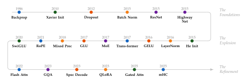
Figure 1 provides a serpentine timeline showing when each trick was introduced, revealing how the field has evolved from the foundational ideas of the 1980s, through the Transformer revolution, to the efficiency innovations that dominate current research.
Trick #1 - Initialize Wisely
Weight initialisation is the first decision a practitioner makes when
building a neural network, and for decades it was one of the most
poorly understood. The consequences of getting it wrong are immediate
and catastrophic: activations explode to NaN within a few
forward passes, or gradients shrink to machine epsilon within a few
backward passes, and the network learns nothing. The consequences of
getting it right are equally dramatic: a well-initialised
100-layer network trains as smoothly as a 5-layer one.
Historical Note.
The dark age of random initialisation. Before 2010, the standard advice for weight initialisation was astonishingly vague: “draw from a uniform distribution, maybe , maybe ; experiment and see what works.” LeCun et al. [1] had noted as early as 1998 that the variance of the weights should be related to the fan-in of each layer, but the recommendation was buried in a long technical report and rarely followed. As a result, deep networks (anything beyond 3–5 layers) routinely failed to train. Researchers attributed the failure to “the difficulty of deep learning” rather than to the mundane cause of poor initialisation.
The breakthrough came in 2010. Glorot and Bengio [2] published a systematic analysis of signal propagation through deep networks, deriving the condition under which activations and gradients neither explode nor vanish. Their “Xavier initialisation” was the first principled scheme, and it immediately enabled the training of networks with 10–20 layers. Five years later, He et al. [3] extended the analysis to ReLU networks, and the era of 100-layer networks began. In retrospect, the key insight is almost embarrassingly simple: match the variance of the weights to the fan-in so that the variance of activations is preserved layer to layer. But this simple idea was the single most important enabler of deep learning.
Variance Propagation Analysis
The central question of initialisation theory is: how does the variance of activations change as a signal propagates through a deep network? To answer it, we analyse a simple linear network (no activation functions) and then extend the analysis to nonlinear networks with ReLU.
Consider an -layer feedforward network with layer widths . At layer , the pre-activation is (Forward Preact) where is the weight matrix and is the activation from the previous layer (with ). We omit biases for clarity; they are typically initialised to zero and do not affect the variance analysis.
Under the assumptions that (i) the weights are i.i.d., (ii) the weights are independent of the activations, and (iii) the activations have zero mean (), the variance of a single pre-activation component is (VAR Single Layer) This is the fundamental variance recursion: the variance at each layer is scaled by a factor of relative to the previous layer.
After layers, the variance accumulates multiplicatively: (VAR L Layers) Each factor acts as a gain: if it exceeds , the variance grows exponentially with depth; if it is less than , the variance shrinks exponentially. Only when for every layer does the variance remain constant.
Remark 1.
The same analysis applies to the backward pass. Let denote the gradient of the loss with respect to the pre-activations. Then (for linear activations), and (VAR Backward) Now the gain factor is : the fan-out replaces the fan-in. For the gradients to be preserved, we need .
We face a tension: the forward pass requires (fan-in), while the backward pass requires (fan-out). These coincide only when , i.e., all layers have the same width. For networks with varying widths, a compromise is needed.
Xavier/Glorot Initialisation
Glorot and Bengio [2] proposed resolving the fan-in versus fan-out tension by taking the harmonic mean.
Definition 1 (Xavier/Glorot Initialisation).
Let and denote the fan-in and fan-out of a layer. Xavier initialisation draws the weights from (Xavier Normal) or equivalently from a uniform distribution (Xavier Uniform) where the uniform bounds are chosen so that the variance matches (Xavier Normal): for a uniform distribution on , .
Proposition 1 (Variance Preservation under Linear Activation).
Under Xavier initialisation with linear activations, the variance of the pre-activations satisfies (Xavier VAR FWD) When , the variance is exactly preserved. More generally, the multiplicative factor remains close to whenever the fan-in and fan-out are of similar magnitude.
Proof.
From the variance recursion (VAR Single Layer), Substituting : When , this reduces to , so the variance is exactly preserved.
For the backward pass, the analogous calculation gives a factor of , which also equals when . The Xavier variance is the unique choice that simultaneously makes both factors as close to as possible; it is the harmonic mean of the forward-only choice and the backward-only choice .
Remark 2.
Xavier initialisation assumes linear (or ) activations, because the derivation relies on and . For , this is approximately satisfied near the origin where . For ReLU, the assumption fails dramatically: half the activations are zeroed out, effectively halving the effective fan-in.
Kaiming/He Initialisation
He et al. [3] observed that for ReLU activations, Xavier initialisation causes the variance to halve at each layer, because ReLU zeroes out negative activations. To compensate, they derived a modified variance that accounts for the ReLU's asymmetry.
The key calculation is the second moment of a ReLU-transformed Gaussian. If , then , and (RELU Second Moment) The integral follows from the half-Gaussian second moment: for a standard Gaussian, , and scaling by gives .
Since for the ReLU (the mean is ), we have (RELU Variance) For the purpose of the initialisation derivation, the simpler bound suffices, because we want for the pre-activations.
Definition 2 (Kaiming/He Initialisation).
For a layer with fan-in and ReLU activation, He initialisation draws the weights from (HE INIT) For the backward-pass variant (“fan-out mode”), the variance is .
The factor of compensates for the ReLU halving: each layer's forward-pass gain is so the variance of the pre-activations is preserved exactly.
Remark 3.
For Leaky ReLU with negative slope , the second moment becomes , and the corrected variance is . Setting recovers He initialisation; setting (the identity function) recovers Xavier with fan-in only.
Orthogonal Initialisation
Xavier and He initialisations control the average variance propagation, but they do not guarantee that all singular values of the weight matrix are well-behaved. A Gaussian random matrix has singular values that follow the Marchenko–Pastur distribution, which means some directions may amplify signals while others suppress them. Orthogonal initialisation eliminates this variability entirely.
Definition 3 (Orthogonal Initialisation).
To initialise a weight matrix :
Generate a random Gaussian matrix with entries .
Compute the thin SVD: .
If , set (the left singular vectors). If , set (the right singular vectors).
The resulting matrix has orthonormal rows (or columns), so (if ) or (if ).
The key property is dynamical isometry : all singular values of are exactly . For a product of orthogonal matrices, , all singular values of the product remain exactly (since the product of orthogonal matrices is orthogonal), so the signal is preserved perfectly, not merely in expectation, but for every input direction.
Saxe et al. [5] proved that orthogonal initialisation produces exact solutions to the learning dynamics of deep linear networks, showing that the training trajectories can be solved in closed form. The gradient flow decomposes along the singular vectors, with each mode converging independently, a remarkable simplification that holds exactly for linear networks and approximately for networks with smooth nonlinearities.
Remark 4.
Orthogonal initialisation produces the theoretically optimal conditioning at the point of initialisation: the condition number of each weight matrix is exactly , and the Jacobian of the entire network has singular values concentrated at . In practice, this advantage is most pronounced for RNNs, where the recurrent weight matrix is multiplied by itself many times (one per time step), making the exponential compounding of non-unit singular values especially damaging. For feedforward networks, orthogonal initialisation provides moderate improvements over He initialisation, particularly for very deep networks ().
Layer-Sequential Unit-Variance (LSUV)
The methods above derive the initialisation variance from theoretical analysis under simplifying assumptions (linear activations, Gaussian inputs, independence). In practice, nonlinearities, batch normalisation, and complex architectures violate these assumptions. Mishkin and Matas [6] proposed a pragmatic alternative: measure the actual variance empirically and correct it.
Algorithm 1: Layer-Sequential Unit-Variance (LSUV) Initialisation.
[H]
- Input: Network with layers, mini-batch of data , tolerance , maximum iterations
- Output: Each layer's output has unit variance
- for
- Initialise with orthogonal initialisation (Definition 3)
- for
- Forward pass: compute activations for the mini-batch through layers
- Compute Variance over all elements and batch samples
- if
- break
- Rescale to achieve unit variance
The algorithm proceeds layer by layer (sequentially), so that when layer is calibrated, layers have already been fixed to produce unit-variance outputs. The orthogonal initialisation in step 2 provides a good starting point; the iterative rescaling corrects for the effects of nonlinearities and architectural peculiarities. In practice, convergence to typically requires only 2–3 iterations per layer.
Remark 5.
LSUV is architecture-agnostic: it works for CNNs, RNNs, and even exotic architectures that defy closed-form variance analysis. The cost is a single forward pass per layer (per iteration), which is negligible compared to the training budget. The main limitation is that it calibrates only the initial variance; as training progresses, the variance may drift. This is where normalisation layers (Trick #3 - Normalise Everything) take over, maintaining stable statistics throughout training.
Fixup Initialisation
For deep residual networks, standard initialisation causes the variance of residual outputs to grow linearly with depth (each residual branch adds variance). Zhang et al. [7] proposed Fixup initialisation: scale the last layer of each residual branch by , where is the total number of residual blocks and is the number of layers per block. This factor ensures that the sum of residual contributions has variance, eliminating the need for batch normalisation entirely. Fixup was demonstrated on ResNets with up to 110 layers, matching the performance of batch-normalised networks without any normalisation layers.
Remark 6.
The Fixup scaling factor is derived from the requirement that , where is the residual function of block . If each is an -layer sub-network with He-initialised weights, then . Scaling the last weight matrix by reduces this to . Setting yields ; the refined exponent accounts for the interaction between multiple layers within each block.
Maximal Update Parameterisation (PmuP)
All the schemes above address a single question: how to start training. Yang and Hu [4] asked a deeper question: how should initialisation, learning rate, and parameterisation co-scale with model width so that the optimal hyperparameters of a small model transfer to a large one?
Standard parameterisation (SP) initialises all layers with the same variance scaling and uses the same learning rate everywhere. Under SP, the optimal learning rate depends on model width: a learning rate that works for a 128-dimensional model is suboptimal for a 1024-dimensional one. This means that hyperparameter tuning must be repeated for every model size, an enormous cost when the target model has billions of parameters.
Definition 4 (Maximal Update Parameterisation (P)).
Let be the model width (hidden dimension). Under the maximal update parameterisation (P), the initialisation scale and learning rate are set per layer type as follows:
1.3
Layer type Init scale () Learning rate () Input embedding Hidden (width ) Output projection
The name “maximal update” reflects the fact that P is the unique parameterisation that (i) ensures stable forward and backward passes and (ii) allows each layer to make the largest possible update without destabilising the network. Under standard parameterisation, hidden-layer updates scale as , which shrinks to zero as the model grows, effectively turning large models into “lazy” networks that learn slowly. Under P, updates remain in the feature space (the space of activations), which is the correct scaling for feature learning.
Proposition 2 (Hyperparameter Transfer under P).
Under P, the optimal learning rate, optimal batch size, and optimal training dynamics are width-independent: if is optimal for a proxy model of width , then is also optimal (up to corrections) for a target model of width .
Proof sketch.
The proof proceeds via the tensor programs framework [4]. The key idea is to track the scaling of every quantity (weights, activations, gradients, updates) as . Under P:
The pre-activations have because .
The weight update has size because and the gradient is .
The resulting change in the pre-activations is : each layer's output changes by a width-independent amount.
Since all quantities are in the infinite-width limit, the loss landscape and its optima are width-independent.
Remark 7.
P allows tuning hyperparameters on a small proxy model (e.g., M parameters) and transferring them directly to a large target model (e.g., B parameters), saving orders of magnitude in compute. Cerebras demonstrated this by tuning on a 40M-parameter model and training a 6.7B-parameter model with the transferred hyperparameters, achieving results competitive with models tuned directly at scale [4].
Visualising Variance Propagation
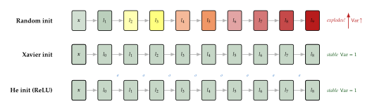
Figure 2 illustrates the effect of different initialisation schemes on the variance of activations as a signal propagates through a 10-layer network.
Comparative Summary
Table 1 summarises the initialisation methods discussed in this section.
| Method | Activation | Property | Year | |
| LeCun [1] | Forward-only | 1998 | ||
| Xavier [2] | Linear / | Fwd + Bwd | 2010 | |
| He [3] | ReLU | ReLU-corrected | 2015 | |
| Orthogonal [5] | Linear | All | Dyn. isometry | 2013 |
| LSUV [6] | Any | Data-driven | Empirical | 2016 |
| Fixup [7] | ReLU (ResNet) | He + | No norm needed | 2019 |
| P [4] | Any | Width-dep. | HP transfer | 2022 |
Key Idea.
The trick is to start in a dynamically neutral state. Every initialisation method in this section pursues the same goal: ensure that signals neither explode nor vanish as they propagate forward through the network (preserving activation variance) and backward through the network (preserving gradient variance). The methods differ in how they achieve this: Xavier uses the harmonic mean of fan-in and fan-out; He compensates for ReLU halving; orthogonal initialisation enforces unit singular values; LSUV measures and corrects empirically; Fixup accounts for residual accumulation; P co-scales initialisation with learning rate for width-independent dynamics. But the underlying principle is universal: at initialisation, every layer should act as a near-isometry, transforming its input without changing its scale. A network initialised in this dynamically neutral state is free to learn; a network initialised poorly is dead before training begins.
Trick #2 - Make It Gated
Gates are the switches of deep learning. A gate is nothing more than a learned function that outputs values between 0 and 1, multiplied element-wise with a signal to selectively amplify or suppress each dimension. This deceptively simple mechanism (multiply by a number between zero and one) turns out to be arguably the single most important trick in the entire field. Gates appear in recurrent networks, feedforward layers, attention mechanisms, and highway connections. Every major architecture breakthrough of the past decade has either introduced a new kind of gate or applied an existing gate in a new place.
Historical Note.
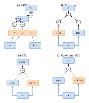
From LSTM gates to gated attention: three decades of gating. The idea of gating information flow traces back to Hochreiter and Schmidhuber's Long Short-Term Memory (LSTM) [8] in 1997, which introduced input, forget, and output gates to control information flow through a recurrent cell. For nearly two decades, the LSTM gate remained the canonical example. Then the pace accelerated: Cho et al. [9] simplified the LSTM into the Gated Recurrent Unit (GRU, 2014) with two gates instead of three. Srivastava et al. [10] introduced Highway Networks (2015), applying gates to feedforward skip connections. Dauphin et al. [11] proposed the Gated Linear Unit (GLU, 2017), gating feedforward layers without recurrence. Shazeer [12] revisited GLU with modern activations (SwiGLU, 2020), creating the feedforward layer now standard in every major LLM. Most recently, Qiu et al. [13] showed that adding a single sigmoid gate to attention heads eliminates attention sinks and dramatically improves long-context performance (Gated Attention, 2025, NeurIPS Best Paper). The trajectory is clear: wherever there is a bottleneck in expressiveness or information flow, adding a gate resolves it.
We met gates in the LSTM (Definition 11), where input, forget, and output gates control information flow through the recurrent cell. Here we formalise the general gating mechanism and trace its evolution through the architectures that define modern deep learning.
The General Gating Mechanism
At its core, every gate has the same structure: project the input, apply a sigmoid, and multiply element-wise.
Definition 5 (General Gating Mechanism).
Given an input , a gating mechanism produces (GATE) where and are learnable parameters, is the logistic sigmoid, and denotes element-wise (Hadamard) multiplication. The gate acts as a learnable soft switch: each dimension is independently amplified (when ) or suppressed (when ).
The gate's power comes from its data dependence: the same network dimension may be opened wide for one input and shut for another. This is fundamentally different from a fixed mask or a global scaling factor. The sigmoid activation is the natural choice because its range makes it interpretable as a “proportion of signal to let through.”
Remark 8.
Why does gating help gradient flow? Consider the gradient of with respect to . By the product rule, (GATE GRAD) The first term provides a direct path for gradients, analogous to the residual connection's identity shortcut. When , gradients flow through unchanged. When , the dimension is suppressed but the second term still provides a learning signal to open the gate.
Highway Networks
Before ResNets, before skip connections became ubiquitous, Srivastava et al. [10] proposed the first architecture to successfully train networks with dozens of layers by using gates to control the information highway.
Definition 6 (Highway Layer).
A highway layer computes (Highway) where is the transform gate, is a nonlinear transformation, and is sometimes called the carry gate.
Remark 9.
Highway networks preceded ResNets [14] by several months. The connection is revealing: when everywhere, (pure transform); when , (pure carry, i.e., identity skip). A ResNet is a special case where everywhere: . The highway network is strictly more expressive because the gate can learn how much to transform versus carry at each layer and each dimension. In practice, however, ResNets' simpler structure proved easier to train at scale, and the extra expressiveness of the highway gate was not needed when combined with batch normalisation.
Gated Recurrent Unit
Cho et al. [9] proposed the GRU as a simpler alternative to the LSTM, reducing three gates to two while retaining comparable modelling power.
Definition 7 (Gated Recurrent Unit).
The Gated Recurrent Unit (GRU) updates its hidden state as follows: (GRU Update) where denotes concatenation, is the sigmoid function, and is element-wise multiplication.
The update gate plays the role of both the LSTM's input gate and forget gate: when , the hidden state is carried unchanged from the previous step (); when , the hidden state is replaced by the candidate . The reset gate controls how much of the previous hidden state to expose when computing the candidate: when , the candidate depends only on the current input, effectively “resetting” the memory.
Remark 10.
Two gates versus three: the GRU has approximately 25% fewer parameters than the LSTM for the same hidden dimension, because it eliminates the output gate entirely (the full hidden state is always exposed). Empirically, neither architecture consistently dominates the other [9]. The GRU tends to perform comparably on tasks with moderate-length dependencies and trains faster due to its reduced parameter count. The LSTM retains an advantage on tasks requiring fine-grained control over what to expose versus what to remember, thanks to its separate output gate.
Gated Linear Units and the SwiGLU Family
Dauphin et al. [11] introduced the Gated Linear Unit for language modelling, demonstrating that gating could accelerate convergence even in non-recurrent architectures. The idea is beautifully simple: split the feedforward computation into two parallel paths, one of which passes through a gate.
Definition 8 (Gated Linear Unit).
The Gated Linear Unit (GLU) is defined as (GLU) where and are learnable parameters, is the sigmoid function, and denotes element-wise multiplication. The left factor is the value path; the right factor is the gate path.
The key insight is that the gate operates on a linear projection of the input: there is no nonlinearity applied to the value path before gating. This “linear” qualifier is what gives the GLU its name and its gradient-friendly properties: the value path preserves a direct linear pathway for gradients.
Shazeer [12] systematically explored replacing the sigmoid gate with other activation functions, discovering that SiLU-gated variants (SwiGLU) consistently outperformed alternatives. Table 2 summarises the family.
| Variant | Gate activation | Introduced by | Used in |
| GLU | Sigmoid | Dauphin et al. [11] | Original paper |
| ReGLU | ReLU | Shazeer [12] | - |
| GEGLU | GELU | Shazeer [12] | GPT-J, GPT-NeoX |
| SwiGLU | SiLU | Shazeer [12] | LLaMA, Qwen, DeepSeek |
SwiGLU (Definition 20) is now the standard feedforward layer in all major open-weight LLMs, including LLaMA, Mistral, Qwen, and DeepSeek. The SwiGLU FFN ((Swiglu)) replaces the traditional two-layer FFN with a three-matrix computation that includes a gated branch, typically using a hidden dimension of (rounded to the nearest multiple of 256) to keep the parameter count comparable to the ungated alternative.
Remark 11.
The gated FFN has three weight matrices (, , ) instead of two, so the parameter count per layer increases unless the hidden dimension is reduced. The standard practice is to set the hidden dimension to rather than : , exactly matching the parameters of the ungated FFN.
Gated Attention: A Deep Dive
Definition 18 defined gated attention; we now examine why it works. Qiu et al. [13] showed that adding a single sigmoid gate to each attention head resolves a fundamental expressiveness bottleneck in multi-head attention and eliminates the infamous “attention sink” phenomenon.
The low-rank bottleneck.
In standard multi-head attention, each head computes (MHA HEAD) where is the softmax-normalised attention weight from token to token , is the value projection, and is the output projection. The effective per-head transformation of the value is , but this matrix has rank at most , where is the number of heads. For a model with and , each head projects through a rank-128 bottleneck. This limits the expressiveness of each individual head.
Five gating positions.
Qiu et al. [13] systematically evaluated five positions for inserting a gate into the attention computation:
G1: Gate after SDPA output. , where is the output of scaled dot-product attention. The gate operates on the full -dimensional output, breaking the per-head low-rank constraint.
G2: Gate value projection. , applied before the attention weighted sum.
G3: Gate key projection. , modulating key representations.
G4: Gate query projection. , modulating query representations.
G5: Gate output projection. , applied after the final linear projection.
Of these, G1 performed best, consistently improving perplexity, long-context recall, and training stability. The reason is geometric: G1 is the only position where the gate operates on the full-rank attention output, allowing it to break the per-head rank bottleneck. Gates at positions G2–G5 operate within the low-rank subspace of individual heads and therefore cannot resolve the fundamental expressiveness limitation.
Proposition 3 (Expressiveness of Gated Attention).
In standard multi-head attention with softmax, the output for token in head lies in the convex hull of the value vectors: (Convex HULL) since and by the softmax normalisation. In gated attention (G1), the output becomes (Gated Output) which can produce outputs outside .
Proof.
In standard attention, the softmax constraints and ensure that is a convex combination of the value vectors, and therefore .
For gated attention, let for some dimension . Then If (i.e., the convex combination attains the minimum value in dimension ), then scaling by produces , which is strictly below the convex hull in dimension . More generally, since is a convex set containing , scaling individual dimensions toward zero can exit the hull whenever the origin is not itself in the hull.
The attention sink problem.
The softmax normalisation forces : the model must attend somewhere, distributing its full attention budget across the available tokens, even when no token is genuinely relevant to the current query. In practice, this forces the model to concentrate excess attention mass on a convenient “dump” token (typically the first token or the beginning-of-sequence token), creating what Xiao et al. [58] termed an attention sink.
Attention sinks are problematic for three reasons:
Wasted capacity: the first token's value vector is mixed into every output, injecting irrelevant information.
KV cache dependency: the first token's key and value must be retained forever, complicating sliding-window and streaming inference.
Long-context degradation: as the context grows, the sink absorbs an increasingly large fraction of the attention mass, diluting the signal from genuinely relevant tokens.
The gate provides an elegant resolution. When no token is relevant, the gate can simply output , producing a near-zero output without needing to “waste” attention mass on a sink token. The model no longer needs a dump token because it has an alternative mechanism for expressing “nothing here is relevant.”
Remark 12.
At 15B MoE scale (400B training tokens), Qiu et al. [13] measured that gated attention reduced the fraction of attention concentrated on the first token from 46.7% to 4.8%, a near-complete elimination of the attention sink phenomenon.
Empirical results.
The gains from gated attention are substantial and consistent across scales:
Perplexity: at 15B MoE / 400B tokens, PPL decreased from 6.026 to 5.761 ().
Long-context recall: on the RULER 128k benchmark, accuracy jumped from 31.65 to 58.82 ( points).
Training stability: gated attention enabled larger learning rates without training divergence, effectively expanding the feasible hyperparameter space.
Overhead: the single sigmoid gate adds fewer than to wall-clock training time.
Insight.
A single sigmoid gate per attention head, costing fewer than 2% of compute, eliminated attention sinks and improved 128k context recall by 27 points. The gate does not change the attention pattern; it changes what the model does with the attention output. By providing a “volume knob” on each dimension, the gate lets the model express “I attended to these tokens but their information is not useful” without corrupting the output with sink-token noise. This is a recurring theme: the most impactful tricks are often the simplest, adding a single nonlinear operation at exactly the right bottleneck.
Trick #3 - Normalise Everything
Deep networks are prone to a fundamental instability: as activations propagate through dozens or hundreds of layers, their magnitudes can drift, growing without bound or collapsing to zero. Even when residual connections (Trick #4 - Add Skip Connections Everywhere) prevent gradient death, the activations themselves may still drift to extreme scales, making optimisation difficult. Normalisation layers solve this by enforcing consistent activation statistics at every point in the network.
BatchNorm (Definition 5), LayerNorm (Definition 6), and RMSNorm (Definition 19) were defined in earlier chapters. Here we explore why normalisation works (the answer is more subtle than originally claimed), survey the full family of normalisation methods, and examine the critical question of where to normalise within a Transformer block.
The Covariate Shift Debate
Historical Note.
The covariate shift hypothesis and the great debate. Ioffe and Szegedy [15] introduced BatchNorm in 2015 with a compelling narrative: training is difficult because the distribution of each layer's inputs changes as the parameters of the preceding layers are updated, a phenomenon they called internal covariate shift. By normalising each layer's inputs to zero mean and unit variance, BatchNorm would stabilise these distributions and accelerate training. The paper was enormously influential: BatchNorm was adopted universally and became a cornerstone of deep learning practice.
Three years later, Santurkar et al. [16] challenged this narrative head-on. Their experiments showed that BatchNorm does not reduce internal covariate shift; in fact, networks with BatchNorm sometimes exhibit more covariate shift than those without it. What BatchNorm actually does, they demonstrated, is something far more fundamental: it makes the loss landscape smoother.
Remark 13 (What Does Batch Normalisation Actually Do?).
Santurkar et al. [16] proved that BatchNorm makes the loss function more Lipschitz-continuous: the gradient varies more smoothly as a function of the parameters. Formally, for a loss and parameters , (Lipschitz) for a smaller Lipschitz constant when BatchNorm is used. This smoothness has a direct practical consequence: a smoother landscape means that the gradient at the current point is a more reliable predictor of what the gradient will be after a step, which in turn means that larger learning rates can be used without the optimiser overshooting and diverging. This, not the reduction of covariate shift, is why BatchNorm enables faster training.
Group Normalisation
BatchNorm's Achilles' heel is its dependence on the batch dimension: the mean and variance are computed across all samples in a mini-batch. When the batch size is small, as in detection and segmentation tasks where high-resolution images consume most of GPU memory, the batch statistics become noisy, and performance degrades sharply. Wu and He [59] proposed Group Normalisation (GN) to eliminate this dependency.
Definition 9 (Group Normalisation).
Given a feature tensor (batch, channels, height, width), divide the channels into groups of size . For each sample and group , define the set of indices . Group Normalisation computes (Groupnorm Stats) and normalises each element as (Groupnorm NORM) followed by learnable affine parameters .
Remark 14.
Group Normalisation is a unifying framework. Setting (a single group containing all channels) recovers Layer Normalisation: the statistics are computed over all channels and spatial dimensions for each sample independently. Setting (each channel is its own group) recovers Instance Normalisation: each channel of each sample is normalised independently. GroupNorm interpolates between these extremes, and is the recommended default for convolutional networks.
Instance Normalisation
Ulyanov et al. [60] introduced Instance Normalisation for neural style transfer, where removing instance-specific contrast information proved essential for transferring artistic styles.
Definition 10 (Instance Normalisation).
Instance Normalisation normalises each channel of each sample independently. For sample and channel , (Instancenorm) where and are the mean and variance computed over the spatial dimensions only: .
Remark 15.
Why does Instance Normalisation help style transfer? Each channel in a convolutional feature map captures a particular visual pattern (edges, textures, colours). The mean of a channel captures the overall “amount” of that pattern in the image, a style-dependent quantity. The variance captures the contrast. By subtracting the mean and dividing by the standard deviation, Instance Normalisation strips away the original image's style-specific statistics, making the features more amenable to being recombined with a different style.
Comparison of Normalisation Methods
| Method | Normalise over | Batch-indep.? | Primary use case |
| BatchNorm | per channel | No | Vision (training) |
| LayerNorm | per sample | Yes | Transformers |
| GroupNorm | per group | Yes | Vision (small batch) |
| InstanceNorm | per channel per sample | Yes | Style transfer |
| RMSNorm | per sample (no mean) | Yes | LLMs |
The trend in the field is clear: modern architectures have moved away from batch-dependent normalisation. Transformers use LayerNorm or RMSNorm exclusively, because batch-level statistics are incompatible with autoregressive generation (batch size 1 at inference) and variable-length sequences. RMSNorm ((Rmsnorm)) has emerged as the preferred choice for large language models because it omits the mean subtraction step, saving approximately 10–15% of the normalisation cost while performing comparably [61].
QK-Norm: Normalising Attention Logits
As model dimension grows, the attention logits can grow unboundedly in magnitude, even with the scaling. Henry et al. [62] proposed a simple fix: normalise the queries and keys before computing attention.
Definition 11 (QK Normalisation).
QK Normalisation applies LayerNorm to the query and key projections before computing the attention scores: (Qknorm) so that the attention computation becomes (Qknorm ATTN) After LayerNorm, each row of and has approximately zero mean and unit variance, which bounds the dot product magnitudes and prevents attention logit explosion.
Remark 16.
Without QK-Norm, the dot product scales as in the worst case (when the vectors are aligned). After normalisation, each vector has norm , and by Cauchy–Schwarz, , but in practice the magnitudes are due to the approximate orthogonality of random high-dimensional vectors. The combination of QK-Norm and the scaling factor ensures that the attention logits remain regardless of model dimension, eliminating a common source of training instability at large scale.
DeepNorm: Scaling Normalisation to 1000 Layers
Standard Post-LN Transformers struggle to train beyond approximately 100 layers due to gradient instability. Wang et al. [17] introduced DeepNorm, a modified normalisation scheme that enables stable training of Transformers with up to 1000 layers.
Definition 12 (DeepNorm).
Let denote the total number of sub-layers (each attention or FFN sub-layer counts as one). DeepNorm modifies the residual connection as (Deepnorm) where is a depth-dependent residual scaling factor, denotes the sub-layer function (attention or FFN), and is initialised with Xavier initialisation scaled by .
The choice of and is not arbitrary; it emerges from an analysis of the expected output magnitude across layers.
Proposition 4 (DeepNorm Stability).
Under DeepNorm initialisation with and , the expected output magnitude remains regardless of depth .
Proof sketch.
Consider the unnormalised residual at layer . At initialisation, the sub-layer output has variance proportional to . After layers (without the LayerNorm renormalisation), the accumulated contribution from the sub-layers has variance (Deepnorm VAR) The residual path contributes a scaling factor of , but the LayerNorm at each step renormalises the hidden state to have unit variance. The perturbation from each sub-layer relative to the normalised residual scales as , so the relative perturbation per layer is . Summing over layers, the total relative perturbation is , ensuring bounded variance throughout the network.
Remark 17.
Using DeepNorm, Wang et al. [17] trained a 1000-layer Transformer that outperformed a standard 200-layer Post-LN Transformer on machine translation, demonstrating that depth alone, when properly stabilised, can improve model quality.
Pre-Norm vs Post-Norm
The question of where to place normalisation within a Transformer block has been debated since the architecture's inception. The two dominant approaches, and a more recent hybrid, differ in a single design choice that has profound consequences for training dynamics.
Post-norm (original Transformer).
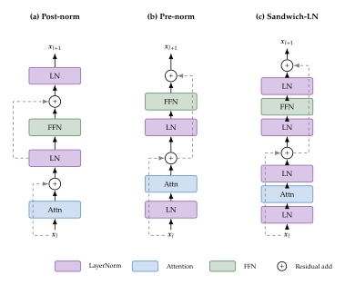
The original Transformer [24] placed LayerNorm after the residual addition: (Postnorm) This was noted in Algorithm 2.
Pre-norm (modern standard).
Most modern Transformers place LayerNorm before the sub-layer: (Prenorm)
Why pre-norm converges faster.
Xiong et al. [63] analysed the gradient flow in both architectures at initialisation and found a crucial difference. In the post-norm configuration, the gradient of the loss with respect to layer must pass through the LayerNorm Jacobian at every subsequent layer. The LayerNorm Jacobian is a projection matrix that subtracts the mean and rescales; this introduces a contraction at each step, causing gradients to shrink as they propagate backward.
In the pre-norm configuration, the residual path provides an unobstructed identity path for gradients. By the chain rule, (Prenorm GRAD) where the identity matrix ensures that the gradient magnitude is at least 1 regardless of depth, analogous to the residual connection's role in gradient preservation.
The quality trade-off.
Despite pre-norm's training advantages, post-norm often achieves better final quality when training succeeds. The reason is subtle: the LayerNorm Jacobian in the post-norm path acts as a form of adaptive regularisation, preventing any single sub-layer from dominating the residual stream. This regularisation effect is lost in pre-norm, where the residual stream is unconstrained and can grow unboundedly, a phenomenon that necessitates the use of a final LayerNorm after the last layer.
Caution.
Changing normalisation order without adjusting the learning rate and other hyperparameters can cause training to diverge entirely. Pre-norm and post-norm architectures have fundamentally different gradient scales at initialisation. A learning rate that is optimal for pre-norm is typically too large for post-norm (causing divergence) or too small for post-norm-to-pre-norm switches (causing slow convergence). When switching normalisation order, always re-tune the learning rate from scratch.
Sandwich normalisation.
A natural question arises: can we get the best of both worlds? The Sandwich-LN configuration adds a second LayerNorm after each sub-layer (but before the residual addition): (Sandwich) The inner LN (pre-norm) ensures stable input to the sub-layer; the outer LN (post-norm) constrains the sub-layer's output magnitude before it enters the residual stream. This prevents the unbounded growth of the residual stream that plagues pre-norm architectures at very large depth. The cost is two additional normalisation operations per block, a negligible overhead at the scale of modern Transformers.
Remark 18.
The practical consensus as of 2025: use Pre-RMSNorm for most LLM applications (fast convergence, simple implementation), QK-Norm when training at large or with FP8 (prevents attention logit explosion), and consider DeepNorm or Sandwich-LN only when pushing to extreme depths ( layers). The original post-norm configuration is rarely used in new architectures.
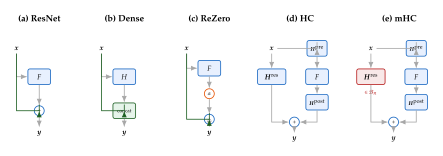
Trick #4 - Add Skip Connections Everywhere
The basic residual block was defined in Definition 9, and the forward pass equation was given in (Residual). In this section we trace the evolution of skip connections from Kaiming He's original insight to the sophisticated multi-stream architectures used in today's largest language models, and explain why the simple act of adding the input back to the output has such a profound effect on trainability.
Historical Note.
He's 152-layer revolution (2015). Before ResNet, networks deeper than roughly 20 layers were essentially untrainable. The problem was not overfitting; deeper networks produced higher training error than their shallower counterparts, a phenomenon He et al. [18] termed the degradation problem. At ILSVRC 2015, He's 152-layer ResNet won every track by a landslide: 3.57% top-5 error on ImageNet (the first superhuman result), first place in detection, first place in localisation. The margin of victory stunned the community. A 56-layer plain network had higher error than a 20-layer one; a 152-layer ResNet dramatically outperformed both.
The key insight was deceptively simple: make it easy for the network to learn the identity function. If the optimal transformation at a given layer is close to the identity, a plain network must learn weights that produce , a nontrivial optimisation target. A residual network need only learn , which is trivially achieved by driving the weights to zero.
Highway networks (Definition 6) preceded ResNets by several months [10], introducing a gating mechanism (Trick #2 - Make It Gated) to control the flow of information along skip paths. But the simplicity of ResNet's ungated additive shortcut proved more influential: no learnable gating parameters, no additional hyperparameters, just . This simplicity enabled scaling to depths that were previously unthinkable.
The Unraveled View of Residual Networks
Veit et al. [64] and Greff et al. [14] offered an elegant reinterpretation: a ResNet is not a single deep computation, but an exponential ensemble of shallow paths.
Proposition 5 (Unraveled View of ResNets).
A residual network of depth can be decomposed into implicit paths of varying lengths. Specifically, the output of the network is (Unraveled) where each subset defines a path through precisely the layers in , and the product is taken in increasing order of indices.
Proof.
Expand the composition directly. For : which has terms corresponding to the four subsets of : (the identity path ), , , and . The general case follows by induction: each additional layer doubles the number of paths by either including or excluding .
The critical empirical finding is that most gradient in practice flows through short paths of length 3–5 layers, not through the full-depth path. This explains why ResNets behave more like ensembles of moderately deep networks than like a single very deep one.
Remark 19.
Removing a single layer from a trained ResNet causes only mild accuracy degradation, consistent with the iterative refinement interpretation, where each layer makes a small correction to the running representation, rather than the hierarchical abstraction view where each layer builds qualitatively new features. This robustness stands in stark contrast to plain networks, where removing any layer causes catastrophic failure.
Pre-activation Residual Blocks
He et al. [65] identified a subtle but consequential design flaw in the original ResNet: the ReLU after the addition corrupts the identity shortcut.
Definition 13 (Pre-activation Residual Block).
The pre-activation residual block applies normalisation and activation before the weight layers: (Preact) where denotes the weight layers (convolutions or linear maps). This contrasts with the post-activation design of the original ResNet: (Postact) The key difference: in (Preact), the skip path carries a pure identity: no nonlinearity on the shortcut.
Why does this matter? The answer lies in the gradient flow.
Proposition 6 (Unimpeded Gradient Flow).
In a pre-activation ResNet with blocks, the gradient of the loss with respect to the activations at layer is (Preact GRAD) The identity term ensures that gradient flows directly from the loss to any layer without multiplicative decay.
Proof.
Since , the Jacobian of each block is . Applying the chain rule from layer to layer : Expanding this product yields a sum of terms, each containing at least one copy of (the direct gradient path). Even if all Jacobians are small, the identity term guarantees a non-vanishing gradient signal.
Remark 20.
In the post-activation design ((Postact)), the ReLU after the addition clips negative values on the skip path, introducing a multiplicative factor that can zero out gradient components. Pre-activation removes this obstruction entirely.
DenseNet: Concatenation Instead of Addition
Huang et al. [66] pushed skip connections to their logical extreme: connect every layer to every preceding layer.
Definition 14 (Dense Block).
In a dense block, the -th layer receives the concatenation of all preceding feature maps as input: (Densenet) where denotes channel-wise concatenation and is a composite function (typically BN–ReLU–Conv). Each layer produces new feature maps, where is called the growth rate. After layers within a dense block, the total number of channels is , where is the number of input channels.
The crucial difference from ResNet is concatenation instead of addition. Addition merges information destructively: two feature maps are collapsed into one. Concatenation preserves all information, allowing later layers to directly access the raw features from any earlier layer. This direct access path encourages feature reuse: later layers can build on features computed at any earlier stage without recomputing them.
Remark 21.
DenseNet achieves comparable accuracy to ResNet with significantly fewer parameters, precisely because of feature reuse. A DenseNet-BC with 0.8M parameters matches the accuracy of a ResNet with 10M parameters on CIFAR-10. The tradeoff is memory: storing all intermediate feature maps for concatenation requires substantially more activation memory during training.
ReZero: Initialise as the Identity
Bachlechner et al. [67] proposed the simplest possible modification to residual connections: multiply the residual branch by a learnable scalar initialised to zero.
Definition 15 (ReZero).
The ReZero connection replaces the standard residual update with (Rezero) where is a learnable scalar initialised to for all layers .
At initialisation, for every layer, so the entire network computes the identity function: for all . The signal propagates through the network without distortion, and the gradients flow back without attenuation. As training progresses, the scalars gradually grow from zero, allowing the network to learn increasingly nontrivial transformations.
Remark 22.
ReZero eliminates the need for learning rate warmup. With standard initialisation, the residual branches produce outputs of magnitude , and these accumulate across layers, creating an signal at the output. Warmup is needed to prevent this accumulated signal from causing instability. ReZero sidesteps the problem entirely: the network starts as the identity and deviates smoothly.
Hyper-Connections: Multi-Stream Residuals
Standard residual connections maintain a single residual stream of dimension . Zhu et al. [68] proposed hyper-connections, which expand the residual stream to parallel copies and mix them through learnable matrices.
Definition 16 (Hyper-Connection).
A hyper-connection expands the residual stream from to dimensions. The update at layer is (Hyperconn) where:
mixes the expanded streams (applied block-diagonally to );
aggregates streams into a single -dimensional layer input;
distributes the -dimensional layer output back to the streams.
The additional expressiveness comes at a cost: the matrices are unconstrained. When composed across layers, their product can have spectral norm far exceeding 1. Zhu et al. measured the Amax Gain, the maximum amplification factor of the residual stream, and found values approaching 3000 in a 27B-parameter Mixture-of-Experts model. Such amplification causes severe training instability: loss spikes, divergent gradients, and wasted compute.
Manifold-Constrained Hyper-Connections
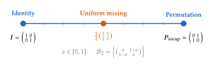
Xie et al. [69] proposed a principled solution: constrain the mixing matrices to the Birkhoff polytope, the set of doubly stochastic matrices.
Definition 17 (Manifold-Constrained Hyper-Connection (mHC)).
A manifold-constrained hyper-connection restricts each in (Hyperconn) to the Birkhoff polytope : (Birkhoff) Each is a doubly stochastic matrix: its rows and columns each sum to 1, and all entries are non-negative.
Doubly stochastic matrices appeared in our treatment of optimal transport (Theorem 2), where the Sinkhorn factorisation theorem establishes that any matrix with positive entries can be scaled to a doubly stochastic matrix by alternating row and column normalisation. Here, the same structure provides stability guarantees for deep residual networks.
Proposition 7 (mHC Stability).
If each , then:
(spectral norm bounded);
(closure under multiplication);
(subsumes standard residual connections).
Proof.
(a) By the Birkhoff–von Neumann theorem, , where is the set of permutation matrices. Permutation matrices are orthogonal, so for all . For with and :
(b) Let . Then , and . Since , we also have . Hence .
(c) , , and , so .
Property (b) is the crucial one: no matter how many layers we stack, the composed mixing matrix remains doubly stochastic with spectral norm at most 1. This eliminates the exponential amplification that plagued unconstrained hyper-connections.
Sinkhorn–Knopp projection.
In practice, the raw parameters are unconstrained. To project onto , we apply the Sinkhorn–Knopp algorithm (Algorithm 1): (MHC Sinkhorn) where divides each row by its sum and divides each column by its sum. The exponential ensures positivity; alternating normalisation converges to a doubly stochastic matrix. In practice, iterations suffice for .
Insight.
The Birkhoff constraint bounds Amax Gain from (unconstrained) to (mHC), while retaining the expressiveness of multi-stream residual connections. The constraint does not eliminate the ability to route information differentially across streams; it merely prevents any stream from being amplified without bound. This is a recurring theme in deep learning: constraints that prevent pathological behaviour often improve both stability and final performance.
Remark 23.
DeepSeek adopted mHC in their latest models, with measurable training stability improvements at 200B+ scale. The overhead of Sinkhorn projection is negligible: for streams, each projection involves a matrix, a cost dwarfed by the attention and feed-forward computations.
Trick #5 - Choose Your Activation Wisely
Standard activations (sigmoid, tanh, ReLU, and their variants) were catalogued in Definition 2. Here we examine the subtleties that make one activation preferable to another, from the pathologies of ReLU to the self-normalising properties of SELU to the empirical dominance of GELU and SiLU in modern large language models.
Historical Note.
From the step function to learned activations: eight decades of evolution. The McCulloch–Pitts neuron (1943) used a binary step function: fire or not. The perceptron (Rosenblatt, 1958) inherited this discontinuity, which made gradient-based learning impossible. The sigmoid and hyperbolic tangent provided smooth, differentiable alternatives that enabled backpropagation (Rumelhart et al., 1986), but both suffered from saturating gradients: for large , the derivative approaches zero, choking gradient flow in deep networks.
Nair and Hinton (2010) introduced the Rectified Linear Unit , which is non-saturating for and computationally trivial. ReLU enabled the training of AlexNet (2012) and became the default activation for nearly a decade. But ReLU has its own pathology, dying neurons, which spawned a menagerie of alternatives: Leaky ReLU, ELU [19], SELU [20], GELU [21], SiLU/Swish [22], and Mish [23]. Today, the “best” activation is often dictated not by theory but by hardware support: GELU and SiLU dominate large-scale training because they are well-optimised on modern GPUs and TPUs.
The Dying ReLU Problem
ReLU's hard zero for creates a pathological failure mode: neurons can become permanently inactive.
Proposition 8 (Dying ReLU).
A ReLU neuron with weights and bias computes . If for every input in the training set, the neuron's output is identically zero, and its gradient . The neuron receives no gradient signal and cannot recover; it is dead.
Proof.
For , we have and . By the chain rule, the gradient of the loss with respect to passes through the factor , which is zero for all training examples. With zero gradient, the parameters and receive no updates, so the neuron remains in the dead state permanently.
Under He initialisation with , the probability of a neuron dying increases with network depth and learning rate. A large learning rate can push the bias term sufficiently negative that for all , killing the neuron in a single update step.
Remark 24.
In practice, 10–20% of neurons can die in deep ReLU networks, especially in the early layers where gradient magnitudes are largest relative to the scale of the weights. This motivated alternatives such as Leaky ReLU ( with ), which ensures a small but non-zero gradient for .
SELU: Self-Normalising Networks
Klambauer et al. [20] designed an activation function that makes explicit normalisation layers unnecessary, by ensuring that activations automatically converge to zero mean and unit variance.
Definition 18 (Scaled Exponential Linear Unit).
The Scaled Exponential Linear Unit (SELU) is defined as (SELU) where and .
The seemingly arbitrary constants and are far from arbitrary; they are the unique solution to a pair of integral equations that enforce the self-normalising property.
Theorem 1 (Self-Normalising Property).
Let and define and . Under LeCun normal initialisation (), the mapping has a stable attracting fixed point at .
Proof sketch.
Let denote the standard normal density. The constants and are chosen as the unique solution to the system (SELU Conditions) The first equation ensures when ; the second ensures . A Banach fixed-point argument on the mapping shows that is a stable attractor: perturbations in mean or variance are contracted back towards the fixed point at each layer.
Remark 25.
SELU achieves self-normalisation without explicit normalisation layers (BatchNorm, LayerNorm, etc.), but only under restrictive conditions: fully connected architectures, LeCun normal initialisation, and no skip connections that break the sequential layer-by-layer structure. For convolutional networks and Transformers, explicit normalisation remains necessary, which limits SELU's practical adoption despite its theoretical elegance.
GELU, SiLU, and the NAS Connection
The two activations that dominate modern large language models are GELU [21] and SiLU (also called Swish) [22]. Recall from (Sigmoid) and (Sigmoid): (GELU Recap) where is the standard normal CDF and is the logistic sigmoid.
These two functions are strikingly similar. The connection is immediate once we note that : the logistic sigmoid is a rescaled approximation to the normal CDF. Substituting: (GELU SILU Relation) In practice, the difference between GELU and SiLU is negligible for most architectures. GPT-2/3 and BERT use GELU; LLaMA and PaLM use SiLU. The choice is often determined by framework defaults rather than principled comparison.
How Swish was discovered.
Ramachandran et al. [22] used neural architecture search (NAS) to search over the space of activation functions parameterised as for learnable . The search, conducted across multiple architectures and datasets, consistently converged to , yielding , the SiLU function.
Insight.
Neural architecture search rediscovered a function that mathematicians would recognise as the logistic-weighted identity. The function is a smooth, non-monotonic approximation to ReLU: it is approximately linear for , approximately zero for , and has a small negative region near (minimum value ). This slight non-monotonicity allows the network to suppress weakly negative signals without completely zeroing them out, a property that appears to improve optimisation.
Mish
Misra [23] proposed another smooth, non-monotonic activation that shares the beneficial properties of SiLU but uses a different mathematical formulation.
Definition 19 (Mish).
The Mish activation is defined as (MISH)
Like SiLU, Mish is smooth, non-monotonic, and unbounded above. It has a slightly deeper negative trough than SiLU (minimum value at ) and approaches the identity more slowly for large . Empirically, Mish performs comparably to SiLU on most benchmarks, with occasional small advantages on vision tasks (it was the default activation in YOLOv4).
StarReLU: Matching GELU Statistics Cheaply
Yu et al. [70] observed that much of GELU's benefit comes from its output statistics (mean and variance), not its precise functional form. They proposed an activation that matches GELU's statistics using only elementary operations.
Definition 20 (StarReLU).
The StarReLU activation is defined as (Starrelu) where and are chosen so that and when , standardising StarReLU to zero mean and unit variance.
StarReLU uses only ReLU and squaring: no exponentials, no error functions, no sigmoid evaluations. On hardware where transcendental functions are expensive (e.g., some mobile accelerators), StarReLU offers a meaningful speedup with minimal accuracy loss. However, on modern GPUs where GELU is implemented as a fused kernel, the computational advantage is negligible, which limits StarReLU's adoption in large-scale training.

Key Idea.
The best activation is often the one your hardware runs fastest. GELU and SiLU dominate large language models not because they are theoretically optimal (no such optimality result exists) but because they are well-supported in fused CUDA kernels on modern GPUs. When choosing an activation, start with GELU (for Transformer-based models) or SiLU (for LLaMA-family architectures). Switch only if profiling reveals a bottleneck: StarReLU for compute-constrained edge deployment, SELU for normalisation-free fully connected architectures, or Mish for specific vision tasks where it has demonstrated gains. The activation function is rarely the limiting factor in model quality; architecture, data, and training procedure matter far more.
Trick #6 - Encode Position Cleverly
Transformers process tokens in parallel, a strength for computation but a weakness for sequence understanding. Unlike recurrent networks, which process tokens one at a time and therefore inherently know the order, a Transformer's self-attention is permutation-equivariant: shuffling the input tokens merely shuffles the output in the same way. Without an explicit position signal, the model cannot distinguish “the cat sat on the mat” from “mat the on sat cat the.”
The sinusoidal positional encoding (Definition 14) and Rotary Position Embeddings (Definition 15), together with the elegant proof that RoPE attention scores depend only on relative position (Proposition 1), were derived in earlier chapters. Here we survey the broader landscape of position encoding strategies, focusing on the practical tricks that determine how far a model can generalise beyond its training context length.
Historical Note.
From afterthought to critical design choice. In the original Transformer paper [24], Vaswani et al. proposed sinusoidal positional encodings almost as an afterthought: the supplementary material showed that learned embeddings performed equally well on their benchmark tasks, and the choice was largely a matter of convenience. GPT-2 (2019) quietly switched to learned positional embeddings, capped at 1024 tokens. It was not until researchers began pushing context lengths beyond a few thousand tokens that the field realised position encoding profoundly affects length generalisation: the ability of a model to process sequences longer than those seen during training.
RoPE [25] (2021) introduced rotary embeddings and quickly became the standard for open-weight large language models. ALiBi [26] (2022) showed that position need not be encoded in the embeddings at all; a simple bias in the attention logits suffices. The NTK-aware scaling trick (2023), discovered by an anonymous Reddit user, and the YaRN method [27] (2023) then showed that RoPE's frequency schedule can be surgically modified to extend context length with minimal fine-tuning. Today, position encoding is recognised as one of the most consequential architectural decisions in language model design.
Learned Positional Embeddings
The simplest alternative to sinusoidal encodings is to learn position representations directly from data.
Definition 21 (Learned Positional Embedding).
Let be the maximum sequence length and the model dimension. A learned positional embedding assigns to each position a trainable vector (Learned PE) where is a learnable embedding matrix initialised at random (typically from ). The input to the first Transformer layer is .
Learned embeddings are maximally flexible: the model can learn arbitrary position-dependent patterns. The fatal limitation is that has exactly rows. At inference time, if the sequence length exceeds , there is no embedding for positions , and the model cannot generalise.
Remark 26.
GPT-2 used ; GPT-3 raised it to . These choices were architectural ceilings that could not be lifted without retraining. This rigidity motivated the search for position encodings with built-in extrapolation capabilities.
ALiBi: Attention with Linear Biases
Press et al. [26] proposed an elegantly simple alternative: do not encode position in the embeddings at all. Instead, add a position-dependent bias directly to the attention logits.
Definition 22 (Attention with Linear Biases (ALiBi)).
Given queries , keys , values , and a head-specific slope , the ALiBi attention for head is (Alibi) where the distance matrix has entries , and the head slopes are set to (Alibi Slopes) with the total number of attention heads.
There are no learnable parameters associated with the position encoding in ALiBi: the slopes are fixed hyperparameters. Different heads attend at different scales: head 1 (the steepest slope) focuses almost exclusively on nearby tokens, while head (the shallowest slope) has a nearly uniform attention pattern.
Proposition 9 (ALiBi Length Extrapolation).
Under ALiBi attention with slope , the unnormalised attention weight from position to position satisfies (Alibi Decay) Thus the attention weight decays exponentially with distance at rate , regardless of the absolute positions involved.
Proof.
Write the softmax input as . By the definition of softmax, The proportionality follows directly. Since the exponential decay factor depends only on the distance and not on the absolute positions or , the attention pattern generalises naturally to positions unseen during training: a token at position attends to a token at position with the same bias as position attends to position .
Remark 27.
ALiBi was used in the BLOOM model (176B parameters) and showed strong length extrapolation: trained at length 2048, it maintained perplexity when tested at lengths up to 8192. However, more recent models have largely converged on RoPE-based approaches, which offer better fine-grained position control.
NTK-Aware RoPE Scaling
Given that RoPE (Definition 15) has become the dominant position encoding, the most pressing practical question is: how do we extend the context length of a pretrained RoPE model without full retraining? The simplest approach, position interpolation [71], linearly rescales all positions by the factor . This works but degrades quality on short-range patterns because it compresses the high-frequency rotations.
Definition 23 (NTK-Aware RoPE Scaling).
Given the original RoPE base frequency , define the NTK-aware scaled base as (NTK ROPE) where is a scaling factor (typically ), is the head dimension, and is the desired context length. The modified frequency schedule is then for .
The key intuition is rooted in the neural tangent kernel (NTK) perspective: the RoPE frequency spectrum spans from very low frequencies (large , capturing long-range structure) to very high frequencies (small , capturing fine-grained local patterns). Position interpolation uniformly compresses all frequencies, destroying the high-frequency information that the model has already learned to use for local token interactions. NTK-aware scaling instead adjusts the base frequency, which effectively stretches the low frequencies more than the high frequencies. The result: long-range positions receive genuinely new frequency representations, while short-range patterns remain largely intact.
Remark 28.
The NTK-aware scaling trick was discovered by an anonymous Reddit user (bloc97) in July 2023 [28] and published as a forum post rather than a peer-reviewed paper. Within weeks, it was adopted by the open-source community and integrated into major inference frameworks. This is a striking example of how the open-source ecosystem can produce and propagate impactful research outside traditional academic channels.
YaRN: Yet Another RoPE ExtensioN
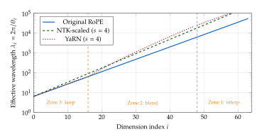
Peng et al. [27] observed that neither pure interpolation nor NTK-aware scaling is optimal across the full frequency spectrum. Their solution, YaRN (Yet Another RoPE ExtensioN), partitions the frequency dimensions into three zones and treats each differently.
Definition 24 (YaRN: Yet Another RoPE ExtensioN).
Let be the extension ratio. For each RoPE dimension , define the wavelength-to-training-length ratio (YARN Ratio) where is the original RoPE frequency for dimension . Given boundary parameters and (typically , ), define the ramp function (YARN RAMP) The three-zone treatment is:
Zone 1 (low frequency, ): interpolate by factor , i.e., .
Zone 2 (mid frequency, ): blend with the ramp function, .
Zone 3 (high frequency, ): keep original frequencies unchanged, .
Additionally, YaRN applies an attention scaling factor (YARN ATTN Scale) to the attention logits, compensating for the entropy increase caused by extending the context window: the query-key dot products are divided by instead of .
The logic behind YaRN's three-zone partition is both simple and elegant. Low-frequency RoPE dimensions encode long-range positional information; since the model has never seen positions beyond , these dimensions must be interpolated. High-frequency dimensions encode short-range patterns that the model has thoroughly learned; modifying them would destroy this learned structure. Mid-frequency dimensions fall somewhere in between and benefit from a smooth blend.
Remark 29.
YaRN achieves 128k context length with only 400 training steps of fine-tuning on a 64k-trained LLaMA model. This remarkable efficiency stems from the fact that YaRN changes only the frequency schedule, not the model weights. The brief fine-tuning allows the model to adapt to the modified frequencies without forgetting its pretrained knowledge.
Position Encoding Comparison
Table 4 summarises the key properties of the position encoding methods discussed in this section and earlier chapters.
| Method | Learned? | Extrapolation | Relative? | Key Property |
| Sinusoidal | No | Limited | No | Fixed; smooth decay with distance |
| Learned | Yes | None | No | Maximum flexibility; fixed |
| RoPE | No | Moderate | Yes | Rotational; decays with distance |
| ALiBi | No | Strong | Yes | Exponential decay via attention bias |
| NTK-RoPE | No | Good | Yes | Frequency-aware base scaling |
| YaRN | No | Strong | Yes | Three-zone frequency modification |
Key Idea.
Position encoding is not just bookkeeping; it determines how far the model can see. The choice of position encoding sets a fundamental limit on context length generalisation. Learned embeddings create a hard ceiling at . Sinusoidal encodings theoretically generalise but degrade in practice. RoPE with intelligent frequency scaling (NTK-aware, YaRN) currently offers the best combination of quality and length extrapolation, which is why nearly all modern large language models use some variant of RoPE.
Trick #7 - Attend Efficiently
Self-attention is the computational heart of the Transformer, but it comes with a quadratic price tag. Standard attention (Definition 12) computes , requiring operations and memory to store the attention matrix. For moderate sequence lengths this is acceptable, but as models push towards million-token contexts, the quadratic cost becomes the dominant bottleneck.
Grouped-query attention (Definition 17), Flash Attention (Algorithm 3) with its IO-complexity analysis (Proposition 2), and multi-head latent attention (Definition 22) were presented in the Transformer chapter. Here we survey additional tricks for taming attention's appetite for compute and memory.
Historical Note.
The quadratic cost of attention is both its strength and its curse. The attention matrix is precisely what allows every token to attend to every other token, a property that gives Transformers their remarkable modelling power. But the cost grows rapidly:
| Sequence length | Attention entries | Scale |
| Manageable | ||
| Expensive | ||
| Very expensive | ||
| Prohibitive |
Sparse Attention Patterns
The simplest idea for reducing attention cost is to compute only a subset of the attention entries. Child et al. [72] introduced systematic sparse attention patterns in the Sparse Transformer.
Definition 25 (Sparse Attention).
Given a sparsity pattern , define the neighbourhood of position as . The sparse attention output at position is (Sparse ATTN) Three canonical sparsity patterns are:
Local window: , with , giving total complexity.
Strided: , with , giving total complexity.
Combined: , combining local detail with long-range connectivity.
Proposition 10 (Sparse Attention Complexity).
Combined local + strided sparse attention with window size and stride achieves complexity, while maintaining the property that every token pair is connected within at most attention hops.
Proof.
Complexity.; Each token attends to at most positions. With , this is . Over all tokens, the total number of attention entries is .
Connectivity.; Let and be arbitrary positions. We show that can reach in at most two hops. Let be the nearest position to that shares a strided connection with (i.e., ). Since , we have , so (hop 1: ). Furthermore, by construction, so (hop 2: ).
Sliding Window Attention
Sliding window attention takes the local window pattern and makes it the primary attention mechanism, relying on the depth of the network to propagate information across the full sequence.
Definition 26 (Sliding Window Attention).
Given a window size , the sliding window attention at position is (SWA) where and denote the key and value vectors for positions in the window . The per-layer complexity is , which is linear in for fixed .
A crucial insight is that the effective receptive field grows linearly with depth. After layers of sliding window attention, information from a token at position can influence a token at position provided . For a model with layers and , the effective receptive field is tokens, sufficient for most practical applications.
Remark 30.
Mistral 7B [29] uses sliding window attention with , augmented by periodic global attention layers (every 4th layer) that attend to the full sequence. This hybrid approach achieves the efficiency of sliding windows while ensuring that long-range dependencies are captured. The Longformer [30] similarly combines local windows with task-specific global attention tokens.
Ring Attention
For sequences so long that even the key-value matrices do not fit on a single accelerator, Ring Attention [73] distributes the computation across multiple devices arranged in a ring topology.
Definition 27 (Ring Attention).
Consider a sequence of length distributed across devices. Each device holds a contiguous block of tokens, with the corresponding query, key, and value sub-matrices . Ring Attention computes exact full attention by circulating the key-value blocks around a ring of devices:
Partition: split the sequence into blocks assigned to devices .
Iterate: for : enumerate[(i)]
Device computes the partial attention of against and .
Device sends its current KV block to device (ring shift).
Accumulate softmax numerators and denominators using the online softmax trick: maintain running max, sum of exponentials, and weighted value sum. enumerate
Finalize: after rounds, each device has computed exact attention for its query block.
Proposition 11 (Ring Attention Communication Cost).
Ring Attention communicates a total of bytes across all devices, achieving linear scaling with the number of devices.
Proof.
In each of the communication rounds (the last round requires no send since each device already holds its own KV block at that point), each device sends a KV block of size values (the factor 2 accounts for both and ). The total bytes communicated across all devices in one round is . Over rounds, the total is . However, since the ring shift is pipelined (each device sends while computing), the latency is rounds, but the bandwidth per device is , independent of .
Remark 31.
Ring Attention is the key enabler for training on extremely long contexts. Combined with Flash Attention for the local computation on each device, it achieves both memory efficiency (via the online softmax trick, which avoids materialising the full attention matrix) and communication efficiency (via the ring topology, which overlaps communication with computation).
Linear Attention
An entirely different approach to reducing attention cost is to approximate the softmax kernel with a decomposable feature map, enabling the computation to be rearranged from to .
Definition 28 (Linear Attention).
Replace the softmax attention with (Linear ATTN) where is a non-negative feature map applied row-wise, and the parenthesisation indicates the order of matrix multiplication. A common choice is , where is the exponential linear unit [31].
The key algebraic insight is the associativity trick. In standard attention, we must first compute (cost ) and then (cost ). In linear attention, we instead first compute (cost ) and then (cost ). The total is , which wins whenever , a common regime in long-context applications.
Remark 32.
Linear attention trades attention quality for computational speed. In practice, the approximation to the softmax kernel is loose, and linear attention models consistently underperform standard softmax attention for language modelling tasks requiring precise token-to-token dependencies. However, linear attention has found success in recurrent-style architectures (RetNet, RWKV, Mamba) where the matrix serves as a compressed state that is updated incrementally, enabling efficient autoregressive inference.
Flash Attention Extensions
The core Flash Attention algorithm was presented in Algorithm 3, with its IO complexity analysis in Proposition 2. Here we survey the subsequent extensions that have made Flash Attention the de facto standard for attention computation.
Flash Attention 2.
Dao [74] introduced several improvements over the original:
Parallelism over sequence length: the original Flash Attention parallelises over batch size and number of heads. Flash-2 additionally parallelises over the sequence length dimension, improving GPU occupancy for long sequences.
Reduced non-matmul FLOPs: by rearranging the online softmax computation, Flash-2 reduces the overhead of non-matrix-multiply operations, which are bottlenecked by GPU register bandwidth.
Result: approximately 2 speedup over the original Flash Attention on A100 GPUs.
Flash Attention 3.
Shah et al. [75] leverage hardware features specific to NVIDIA Hopper GPUs (H100):
TMA (Tensor Memory Accelerator): asynchronous data movement between global memory and shared memory.
WGMMA (Warpgroup Matrix Multiply-Accumulate): higher-throughput matrix multiply instructions.
Warp specialisation: dedicating different warp groups to different tasks (data loading vs. computation) to maximise pipeline utilisation.
Result: 1.5–2 speedup over Flash-2 on H100 GPUs, approaching the theoretical peak throughput.
PagedAttention.
Kwon et al. [76] address a different bottleneck: the KV cache (Definition 16) memory management during inference.
Problem: standard KV cache pre-allocates contiguous memory for the maximum sequence length, leading to significant memory fragmentation and waste when serving multiple requests of varying lengths.
Solution: PagedAttention manages the KV cache in fixed-size pages (analogous to OS virtual memory), allocating pages on demand and using a page table for indirection.
Result: near-zero memory waste, enabling 2–4 higher serving throughput via better batching.
Remark 33.
Flash Attention is an implementation trick, not an approximation: it computes exact attention with the same numerical output as the naive algorithm (up to floating point non-associativity). This is what distinguishes it from sparse or linear attention methods, which sacrifice accuracy for speed. Flash Attention achieves its gains purely through better memory access patterns, a vivid demonstration that algorithms must be designed for the hardware they run on.
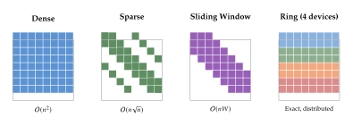
Insight.
The best attention trick depends on the bottleneck. If the bottleneck is memory bandwidth (the attention matrix does not fit in SRAM), use Flash Attention. If the bottleneck is FLOPs (the quadratic computation is too expensive), use sparse attention patterns. If the bottleneck is device memory (the sequence does not fit on a single accelerator), use Ring Attention. In practice, these tricks compose: a modern training run might use Flash Attention locally, sparse patterns for extremely long sequences, and Ring Attention to distribute across a cluster.
Trick #8 - Regularize Creatively
Deep networks have enormous capacity, far more parameters than training examples in most practical settings. Classical learning theory would predict catastrophic overfitting. Yet deep networks generalise remarkably well, and a key reason is the regularisation tricks that prevent them from memorising the training data. This section surveys the most important regularisation techniques, unified by a common principle: inject controlled noise during training, and remove it during inference.
Historical Note.
Hinton's insight: if a committee of experts always agrees, they might be overfitting. Geoffrey Hinton motivated dropout with an analogy from evolutionary biology: sexual reproduction creates genetic diversity by randomly combining parental genes, preventing any single gene from becoming a “free rider” that only works in combination with specific other genes. Analogously, dropout forces each neuron to be independently useful, preventing co-adaptation. Hinton later remarked that this idea came to him after a conversation with a bank teller: banks rotate tellers between branches specifically to prevent fraud through collusion. If employees cannot rely on having the same colleagues, they cannot develop exploitative partnerships. The same principle applies to neurons in a neural network.
Dropout
Definition 29 (Dropout).
Let be a hidden activation vector and the dropout rate. During training, inverted dropout produces (Dropout) where the mask is sampled independently for each neuron and each training example. During inference, no masking or scaling is applied: .
The scaling factor in inverted dropout ensures that the expected value is preserved: . This eliminates the need to modify the network at test time, a practical convenience that has made inverted dropout the universal implementation.
Proposition 12 (Dropout as Implicit Ensemble).
A network with layers, each containing neurons, trained with dropout rate , implicitly trains an ensemble of up to sub-networks. The inference-time prediction (using all neurons with scaled weights) approximates the geometric mean of the predictions of these sub-networks.
Proof sketch.
Each dropout mask selects a sub-network by zeroing out a subset of neurons. Training with dropout optimises the expected loss over masks: For the cross-entropy loss , this is equivalent to minimising the KL divergence to a mixture model. At inference, using all neurons with weights scaled by computes a single forward pass whose output approximates the geometric mean of the sub-network predictions. The approximation relies on the first-order Taylor expansion of the network output around the mean activation, which is exact for linear networks and approximate for nonlinear ones.
Proposition 13 (Dropout as Approximate Bayesian Inference).
Gal and Ghahramani [32] showed that training a neural network with dropout and regularisation is mathematically equivalent to approximate variational inference in a deep Gaussian process. The dropout rate corresponds to the prior precision, and Monte Carlo dropout at test time (running the network multiple times with different dropout masks) provides a principled estimate of predictive uncertainty.
Proof sketch.
Consider a single-layer network with dropout applied to the weight matrix: , . The variational distribution is . Gal and Ghahramani show that the ELBO (evidence lower bound) of this variational distribution, applied to a Gaussian process prior with kernel , equals (up to a constant) the dropout training objective , where is determined by and the prior precision.
DropPath (Stochastic Depth)
Dropout zeros out individual neurons. DropPath, also known as stochastic depth [77], operates at a coarser granularity: it drops entire layers (more precisely, entire residual branches).
Definition 30 (Stochastic Depth / DropPath).
In a residual network with blocks, the output of layer is (Droppath) where is a binary random variable with survival probability that follows a linear decay schedule: (Droppath Schedule) with the survival probability of the last layer (typically ). Early layers (small ) survive with high probability; later layers are dropped more frequently.
At inference, no stochastic dropping is performed. Instead, the residual branch is scaled by the survival probability: (Droppath Inference)
The linear decay schedule reflects the empirical observation that later layers in deep networks tend to learn more fine-grained, task-specific features that are more prone to overfitting, while early layers learn general features that should always be active.
Remark 34.
DropPath is standard in Vision Transformers. DeiT, Swin Transformer, and ConvNeXt all use DropPath with survival rates between 0.7 and 0.9. It is generally more effective than standard dropout for deep residual networks because it regularises the depth of the effective network rather than individual neurons, providing a qualitatively different form of noise injection.
Label Smoothing
Definition 31 (Label Smoothing).
Given classes, replace the hard target (a one-hot vector for class ) with the smooth target (Label Smooth) where is the smoothing parameter (typically ) and [33].
With hard targets, the cross-entropy loss drives the logits towards for the correct class and for all others; the model becomes maximally confident and often overconfident, assigning near-zero probability to all but the correct class. Label smoothing prevents this by ensuring the target distribution always has non-zero probability for every class.
Proposition 14 (Label Smoothing and Calibration).
With label smoothing parameter and classes, the maximum logit at the optimum of the smoothed cross-entropy loss is bounded: (Label Smooth Logit)
Proof.
At the optimum of , the softmax outputs equal the targets: for all . For the correct class , . For incorrect classes, . Using and , we get Taking logarithms: . Since is the maximum logit and all are equal (by symmetry of the target over incorrect classes), this is the maximum logit gap. The bound follows from noting that incorrect classes share the remaining probability mass.
Mixup
Definition 32 (Mixup).
Given two training examples and , Mixup [34] constructs a virtual training example by linear interpolation: (Mixup) where with (typically ).
Remark 35 (Vicinal Risk Minimisation).
Standard empirical risk minimisation (ERM) optimises the loss over point masses at training examples: . Mixup instead minimises risk over the vicinity of training examples, defined by linear interpolation in both input and label space. This vicinal risk minimisation (VRM) framework encourages the model to behave linearly between training examples: the function value at the midpoint of two inputs should be the midpoint of their labels. This implicit linear prior is a powerful inductive bias that reduces oscillation and improves generalisation.
CutMix
Definition 33 (CutMix).
Given two images and their labels , CutMix [35] constructs a training example by spatial composition: (Cutmix) where is a binary mask corresponding to a randomly sampled rectangular region, and is the fraction of the image from .
CutMix offers two advantages over standard Mixup. First, it preserves local spatial structure: within each region, the pixels come from a single coherent image, so the model sees realistic local patterns rather than ghost-like superimpositions. Second, it forces the model to classify from partial information: a training example might show 70% of a dog and 30% of a cat, requiring the model to recognise both from incomplete evidence. This encourages attention to distributed features rather than reliance on a single discriminative region.
R-Drop
Definition 34 (R-Drop).
Given an input and target , pass through the model twice with different dropout masks, producing output distributions and . The R-Drop loss [36] is (Rdrop) where controls the strength of the consistency regularisation, and the symmetric KL divergence penalises the two forward passes for producing different outputs.
Remark 36.
R-Drop combines the ensemble benefit of dropout with a consistency objective. The two forward passes with different masks produce different predictions; the KL term forces these predictions to agree. This is conceptually similar to self-distillation: each forward pass serves as both student and teacher to the other. The result is a model that is more robust to the specific dropout mask used, leading to better generalisation.
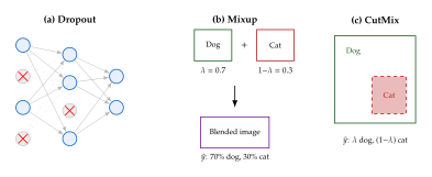
Key Idea.
Regularisation tricks all share one principle: inject controlled noise during training, remove it during inference. Dropout injects noise by zeroing activations. DropPath injects noise by skipping layers. Label smoothing injects noise into the targets. Mixup and CutMix inject noise by blending examples. R-Drop injects noise through inconsistent dropout masks and then penalises the inconsistency. In each case, the noise prevents the model from relying too heavily on any single feature, co-adaptation, or memorised pattern, forcing it to learn robust representations that transfer to unseen data.
Trick #9 - Schedule the Learning Rate
The learning rate in SGD (Definition 4) and its variants is not merely a hyperparameter to be tuned once and fixed. It is a dynamic control signal that shapes the entire training trajectory. Too high, and the optimiser overshoots and diverges. Too low, and it gets trapped in poor local minima or takes unacceptably long to converge. The art of learning rate scheduling is to navigate between these extremes throughout the training process.
Historical Note.
From fixed learning rates to sophisticated schedules. Yann LeCun wrote in 1998: “The learning rate is the single most important hyperparameter, and one should always make sure that it has been tuned.” Early practitioners used a simple prescription: start with a “large” learning rate (e.g., 0.1) and divide by 10 every time the validation loss plateaus (step decay). This worked reasonably well for small networks but required constant manual intervention.
The modern era of learning rate scheduling began with two parallel developments. Loshchilov and Hutter [37] introduced cosine annealing with warm restarts, providing a smooth, principled schedule. Smith [38] showed that cyclical learning rates, deliberately increasing the LR during training, could actually improve convergence. Today, every competitive large-scale training run uses a carefully designed schedule, typically combining warmup, a main training phase, and a cooldown.
Warmup
Definition 35 (Linear Warmup).
During the first training steps, the learning rate increases linearly from near zero to its maximum value: (Warmup) After the warmup phase completes, the learning rate transitions to the main schedule (cosine, linear decay, etc.).
Why is warmup necessary? At initialisation, the network's representations are essentially random. Gradients computed on these random representations are noisy: they point in roughly the right direction on average, but with high variance. A large learning rate applied to noisy gradients produces large, erratic updates that can push the parameters into regions of the loss landscape from which recovery is difficult or impossible.
Proposition 15 (Warmup and Gradient Noise).
Define the gradient noise scale (GNS) as , where is the gradient norm and is the standard deviation of the gradient estimate. The GNS is typically smallest at initialisation (high noise relative to signal). Linear warmup maintains an approximately constant effective step size by keeping the product bounded during the initial phase when is small and growing.
Proof sketch.
At initialisation, the gradients are approximately isotropic with magnitude , so . As training progresses and the network begins to fit the data, the signal-to-noise ratio improves: grows. If were immediately set to , the effective step size would be large. With linear warmup, starts small and grows in proportion to , approximately matching the growth rate of and keeping bounded.
Remark 37.
Every modern large language model training run uses warmup, typically spanning 1–5% of total training steps. The exact warmup duration is not critical: 500 to 5000 steps usually suffices. What matters is that the initial learning rate is small enough to prevent divergence. Goyal et al. [39] demonstrated that warmup is essential for large-batch training: without it, increasing the batch size (and proportionally the learning rate) leads to training instability.
Cosine Annealing
Definition 36 (Cosine Annealing).
The cosine annealing schedule [37] decays the learning rate following a half-cosine curve: (Cosine) where is the minimum learning rate (often or ) and is the total number of training steps.
The cosine schedule has several appealing properties. It starts at when and smoothly decays to when , with no abrupt transitions. Crucially, the schedule spends more time at low learning rates: the derivative is smallest near the endpoints, meaning the learning rate changes slowly at the beginning and end. This is desirable because the final phase of training benefits from small, precise updates.
Cosine with warm restarts (SGDR).
Loshchilov and Hutter also proposed periodically restarting the cosine schedule: (SGDR) where resets to at each restart, and the period can grow geometrically: for the -th restart. Each restart allows the optimiser to escape local minima by temporarily increasing the learning rate, then fine-tune into a (potentially better) basin.
Remark 38.
Cosine annealing (without restarts) is the de facto default schedule for large-scale pretraining of both vision and language models. Chinchilla (2022), LLaMA (2023), and Gemma (2024) all use cosine schedules. The simplicity and robustness of the cosine curve (no step sizes, no milestone epochs) make it an excellent default choice when a practitioner has no strong prior about the optimal schedule.
Cyclical Learning Rates
Smith [38] made a counterintuitive observation: periodically increasing the learning rate during training can improve both convergence speed and final accuracy.
Definition 37 (Cyclical Learning Rate).
The learning rate oscillates between and in a triangular wave with half-period (step size) : (Cyclical LR) The learning rate linearly increases for steps, then linearly decreases for steps, and repeats.
A key practical contribution from Smith's work is the LR range test, a simple diagnostic for finding the viable range of learning rates for any model and dataset.
Definition 38 (LR Range Test).
Start with a very small learning rate (e.g., ).
Increase the learning rate exponentially after each mini-batch: where (e.g., ).
Record the training loss at each learning rate.
Choose as the learning rate where the loss begins to increase (or diverge).
Choose .
Remark 39.
The LR range test is useful for any schedule, not just cyclical. It identifies the viable learning rate range in a fraction of a training epoch, providing an informed starting point that eliminates much of the guesswork in hyperparameter tuning.
One-Cycle Policy
Smith and Topin [78] refined cyclical learning rates into the one-cycle policy, which uses a single cycle of increasing and decreasing learning rate over the entire training run.
Definition 39 (One-Cycle Policy).
The one-cycle schedule has three phases:
Phase 1 (30–50% of training): increase the learning rate linearly from to .
Phase 2 (50–70% of training): decrease the learning rate linearly from to .
Phase 3 (final 5% of training, optional): anneal the learning rate from to a very small value for final fine-tuning.
Concurrently, the momentum parameter (in SGD with momentum) is varied inversely: high momentum when LR is low, low momentum when LR is high.
Insight.
Super-convergence. Smith and Topin demonstrated a remarkable phenomenon: the one-cycle policy can achieve the same final accuracy as a standard schedule in as few as 1/10 of the epochs. This “super-convergence” occurs because the increasing learning rate in Phase 1 serves as a form of regularisation (the large LR prevents the model from settling into sharp minima) while the decreasing phase allows fine-grained convergence to a flat minimum with good generalisation.
WSD: Warmup-Stable-Decay
The most recent addition to the learning rate schedule repertoire is the WSD (Warmup-Stable-Decay) schedule, which was instrumental in training the MiniCPM models [79].
Definition 40 (Warmup-Stable-Decay (WSD) Schedule).
The WSD schedule consists of three phases:
Warmup (): .
Stable (): (constant).
Decay (): , or alternatively, linear or exponential decay.
The key insight behind WSD is that the stable phase at constant serves as a plateau during which the model steadily improves. At any point during the stable phase, one can branch off a copy of the training run and apply a short decay phase to produce a usable checkpoint. This makes the schedule “anytime optimal”: you do not need to commit to a total training budget in advance. With cosine annealing, the learning rate is entangled with the total number of steps , making it impossible to extend training without restarting the schedule.
Remark 40.
The WSD schedule was used to train MiniCPM-2B, a 2.4B parameter model that matches the performance of models 5–10 larger. The authors attribute part of this success to the ability to select the optimal point to begin the decay phase by monitoring validation loss during the stable phase. This “training-as-exploration” paradigm, where the stable phase explores the loss landscape and the decay phase exploits the best trajectory, represents a conceptually clean separation of concerns.
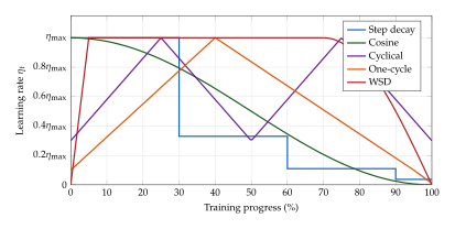
Key Idea.
The learning rate is not a fixed hyperparameter; it is a dynamic control signal that must be matched to the training dynamics. At initialisation, when gradients are noisy and the loss landscape is poorly conditioned, the learning rate should be small (warmup). During the main training phase, it should be large enough to explore broadly. Towards the end, it should decay to allow convergence to a precise minimum. The specific schedule (cosine, cyclical, WSD) matters less than the principle: adapt the learning rate to the training dynamics, not the other way around.
Trick #10 - Train in Low Precision
Every number in a neural network (every weight, activation, gradient, and optimizer state) is represented as a floating-point number. For decades, the default was 32-bit floating point (FP32), a format designed for scientific computing with 7 decimal digits of precision. Modern deep learning has shown that this precision is vastly more than needed: networks can be trained with 16-bit or even 8-bit numbers with little or no accuracy loss, while enjoying dramatic speedups and memory savings.
Historical Note.
The assumption that neural networks need 32-bit precision was one of deep learning's most expensive misconceptions. In 2017, NVIDIA's V100 GPU introduced Tensor Cores with native FP16 support, offering the throughput of FP32 matrix multiplications. Micikevicius et al. [40] (2018) demonstrated that mixed-precision training, using FP16 for most operations while keeping a master copy of weights in FP32, achieved speedup with no accuracy loss across a range of tasks. The A100 GPU (2020) added BF16 (bfloat16) support, a format that trades precision for range, and BF16 quickly became the default for large language model training. The H100 GPU (2022) introduced FP8 Tensor Cores, and FP8 training is now an active area of research, promising yet another throughput improvement.
The progression from FP32 to FP16 to BF16 to FP8 represents one of the most impactful “free lunches” in deep learning: the same model, the same algorithm, the same accuracy, just faster and cheaper.
Floating Point Formats
Definition 41 (IEEE Floating Point Formats).
A floating-point number is represented as (FP Format) where is the sign bit, is the exponent (an unsigned integer), is a format-dependent offset, is the mantissa (significand), and is the number of mantissa bits. The key formats used in deep learning are:
| Format | Sign | Exponent | Mantissa | Range | Precision |
| FP32 | 1 | 8 | 23 | 7 decimal digits | |
| FP16 | 1 | 5 | 10 | 3.3 decimal digits | |
| BF16 | 1 | 8 | 7 | 2.4 decimal digits | |
| FP8 E4M3 | 1 | 4 | 3 | 1.4 decimal digits | |
| FP8 E5M2 | 1 | 5 | 2 | 1.0 decimal digit |
The critical trade-off is between range (determined by the number of exponent bits) and precision (determined by the number of mantissa bits). FP16 has more mantissa bits than BF16 (10 vs. 7), giving it better precision, but FP16's 5-bit exponent limits its range to . BF16 has the same 8-bit exponent as FP32, giving it the same dynamic range (), at the cost of reduced precision.
For training, BF16's range advantage is decisive. Gradient values in deep networks can span many orders of magnitude, and a format that overflows at (FP16) frequently encounters numerical issues during training of large models. BF16 never overflows in practice, making it far more robust.
Caution.
FP16 training of models with more than 1B parameters often diverges due to overflow and underflow. The maximum representable FP16 value is ; any gradient or activation exceeding this value overflows to infinity, corrupting the entire training run. Conversely, gradients smaller than underflow to zero, causing many parameters to stop learning. For large-scale training, use BF16 or FP16 with loss scaling (see below).
Mixed Precision Training
Definition 42 (Mixed Precision Training).
Mixed precision training [40] maintains a master copy of the model parameters in FP32 and performs forward and backward passes in a lower precision format (FP16 or BF16). The training loop proceeds as follows:
Cast: copy the FP32 weights to reduced precision .
Forward: compute the loss in reduced precision.
Loss in FP32: cast the scalar loss to FP32 for numerical stability.
Backward: compute gradients in reduced precision.
Update: cast gradients to FP32 and update the master weights: .
Why keep master weights in FP32? The issue is precision of accumulation. When the learning rate is small (e.g., ) and the gradient is also small, the update may be smaller than the FP16/BF16 precision at the scale of the weight. Concretely, if a weight and the update is , FP16 cannot represent because the mantissa only has 10 bits of precision. In FP32, the 23-bit mantissa resolves this fine difference.
Definition 43 (Mixed Precision Training Loop with Loss Scaling).
Input: model parameters (FP32), loss scale .
.
[FP16 compute]
[scale up to prevent gradient underflow]
[FP16 gradients]
[unscale in FP32]
[FP32 update]
Proposition 16 (Memory Savings of Mixed Precision).
Mixed precision training with FP16/BF16 activations reduces activation memory by approximately compared to FP32, and enables 2 throughput on tensor cores that natively support reduced-precision matrix multiplications.
Proof.
Each FP16/BF16 value requires 2 bytes vs. 4 bytes for FP32, yielding a reduction in memory for activations and temporary buffers. The master weights in FP32 add bytes (where is the parameter count), and the FP16 copy adds bytes, for a total parameter memory of bytes. However, for large models, activation memory dominates parameter memory (especially with long sequences), so the net saving approaches .
The throughput gain comes from GPU tensor cores: NVIDIA A100 tensor cores achieve 312 TFLOPS in FP16/BF16 vs. 156 TFLOPS in FP32 (TF32), a improvement. H100 tensor cores further improve this to 989 TFLOPS in FP16 vs. 495 TFLOPS in TF32.
Loss Scaling
Definition 44 (Dynamic Loss Scaling).
FP16 gradients smaller than underflow to zero, causing the corresponding parameters to stop receiving gradient updates. Loss scaling addresses this by multiplying the loss by a large factor before the backward pass, which shifts all gradients into the representable range, and then dividing by after casting to FP32: (LOSS Scaling) Dynamic loss scaling adapts during training:
Initialise (a large value).
If any gradient is
inforNaN(overflow detected): skip the update and halve .If consecutive steps (e.g., ) pass without overflow: double .
Dynamic loss scaling is automatic: the scale self-adjusts to keep gradients in the representable range of FP16 without requiring any manual tuning. Note that with BF16 training, loss scaling is typically unnecessary because BF16's large dynamic range prevents both overflow and most underflow.
Gradient Clipping
Large gradient norms, caused by outlier examples, loss spikes, or numerical instability, can destabilise training. Gradient clipping constrains the gradient magnitude before the parameter update.
Definition 45 (Gradient Clipping by Norm).
Given a gradient vector and a clipping threshold , the clipped gradient is (GRAD CLIP)
Proposition 17 (Clipping Preserves Gradient Direction).
Gradient clipping by norm preserves the gradient direction: . Only the magnitude is affected: .
Proof.
There are two cases:
If : then , so . Direction and magnitude are unchanged.
If : then . The direction is , which is identical to the original direction. The magnitude is .
In both cases, , and .
Remark 41.
Most large language model training runs use gradient clipping with . This is a conservative choice that rarely clips during normal training (typical gradient norms are well below 1.0 for well-initialised models with proper learning rate schedules) but provides a safety net against the occasional gradient spike that could otherwise cause a loss divergence. Gradient clipping is particularly important when combined with mixed precision training, where reduced-precision gradients are more susceptible to numerical outliers.
Gradient Accumulation
Modern training often requires large effective batch sizes for stable convergence, but GPU memory may only accommodate a small batch. Gradient accumulation bridges this gap by spreading a single optimiser step across multiple forward-backward passes.
Definition 46 (Gradient Accumulation).
To simulate an effective batch size using micro-batches of size , accumulate gradients over micro-batches before performing a single parameter update: (GRAD Accum) where is the -th micro-batch. The parameter update is then .
Proposition 18 (Equivalence to Large-Batch Training).
Gradient accumulation over independent micro-batches of size produces the same expected gradient as a single batch of size : (GRAD Accum Equiv) Moreover, if the micro-batches are drawn independently, the variances are identical: .
Proof.
By linearity of expectation: This is identical to the expected gradient of a single batch of any size, since the expectation is taken over the data distribution.
For the variance, the accumulated gradient over i.i.d. micro-batches of size is the mean of i.i.d. per-example gradients: . A single large batch of size computes . These are the same sum, so , where is the per-example gradient variance.
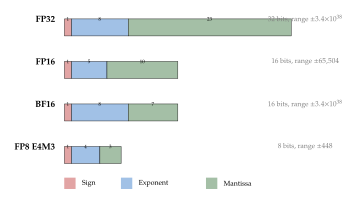
Key Idea.
Modern LLM training runs in BF16 with FP32 master weights, the best of both worlds. BF16 provides throughput and memory savings for forward and backward passes, while the FP32 master weights ensure that tiny gradient updates are not lost to reduced-precision rounding. Combined with gradient clipping (to prevent outlier gradients from destabilising training) and gradient accumulation (to simulate large batch sizes on limited hardware), this low-precision recipe enables training of models with hundreds of billions of parameters on clusters of commodity GPUs. The lesson is clear: precision is a resource to be managed, not an absolute requirement. Use just enough precision where it matters (weight updates) and economise everywhere else (activations, gradients).
Trick #11 - Distill Knowledge
A large model trained for weeks on thousands of GPUs captures an extraordinary amount of knowledge, not merely the mapping from inputs to correct labels, but the relative confidences across all possible outputs. When a vision model assigns probabilities to the classes [cat, lynx, dog], the non-zero probability on “lynx” encodes a structural similarity between cats and lynxes that the hard label entirely discards. Knowledge distillation is the art of transferring this richer signal from a large teacher to a small student.
Historical Note.
Hinton's “dark knowledge” (2015). The idea of model compression via soft targets dates to Bucilua et al. (2006) [41], but the modern formulation is due to Hinton, Vinyals, and Dean (2015) [42], who coined the evocative term dark knowledge: “The knowledge is not just in the hard labels; it is in the relative probabilities of incorrect classes.” A teacher's output tells the student that class 2 is more similar to class 1 than class 3 is. This “dark knowledge” is lost when training on hard labels . By raising the softmax temperature, even tiny probabilities become visible, revealing the full geometry of the teacher's learned representation.
The distillation objective
The core idea is simple: train the student to match both the true labels and the teacher's soft predictions.
Definition 47 (Knowledge Distillation).
Let and denote the logits of a student network and a teacher network, respectively, for a -class classification problem. The knowledge distillation loss is (KD LOSS) where is the softmax function, is the one-hot ground truth, is the temperature parameter, is the interpolation weight, and is the Kullback–Leibler divergence. The first term trains the student on hard labels; the second aligns it with the teacher's softened predictions.
The temperature controls the “softness” of the probability distribution. At , we recover the standard softmax; as , the distribution approaches uniform, revealing the full ranking over classes. The factor in (KD LOSS) is not arbitrary; it compensates for the gradient scaling introduced by the temperature.
Proposition 19 (Temperature and Gradient Scaling).
As , the softened targets approach the uniform distribution . The gradient of the KL term with respect to the student logits scales as for large , which is compensated by the prefactor, yielding an effective learning signal of order .
Proof.
For large , a first-order expansion gives where . Substituting into the KL divergence, Taking the gradient with respect to : Multiplying by , the effective gradient becomes , which is independent of . Thus the factor ensures a stable learning signal regardless of temperature.
Remark 42.
In practice, works well. Small preserves the teacher's sharp predictions (useful when the teacher is highly confident); large reveals fine-grained inter-class similarities (useful when classes are semantically related, e.g., fine-grained visual recognition).
Self-distillation and Born-Again Networks
A surprising finding: distillation improves performance even when the student has the same architecture as the teacher.
Definition 48 (Self-Distillation).
Self-distillation trains a student with the same architecture as the teacher. Starting from a trained model , each generation trains a new model by minimising the distillation loss: (SELF Distill) Furlanello et al. (2018) [43] showed that Born-Again Networks, students identical to their teachers, consistently outperform the teacher, often by – accuracy on ImageNet.
Remark 43.
Why does self-distillation help? The teacher's soft labels act as a form of label smoothing (Trick #8 - Regularize Creatively) and implicit data augmentation: each training example carries soft targets instead of a single hard label, effectively multiplying the information per sample. The teacher also provides a form of curriculum: early in training, the student receives well-calibrated targets that are easier to learn from than noisy hard labels.
Online distillation
Classical distillation requires a pre-trained teacher. Online distillation removes this requirement by training teacher and student simultaneously.
Definition 49 (Deep Mutual Learning).
In deep mutual learning [44], two (or more) networks train simultaneously, each distilling from the other. The losses are (Mutual1) where is the softmax output of network . No pre-trained teacher is needed; the networks learn collaboratively, each providing complementary dark knowledge to the other.
Remark 44.
Remarkably, deep mutual learning improves both networks relative to training each independently, even when both networks have the same architecture and capacity. The KL terms encourage the networks to agree, which acts as a consensus regulariser that reduces overfitting and explores a broader set of good solutions.
Distillation at scale
Insight.
Distillation as the deployment pipeline. Distillation is the primary mechanism by which frontier model knowledge flows into small, deployable models. GPT-4 knowledge is distilled into Phi-series models; LLaMA-70B is distilled into LLaMA-8B variants; PaLM-540B is distilled into Gemma-2B. In the modern LLM ecosystem, distillation is not an afterthought; it is the deployment strategy [41].
Key Idea.
Why distillation works. The teacher provides a richer learning signal than labels alone: inter-class similarities (dark knowledge), confidence calibration (soft targets reveal uncertainty), and implicit data augmentation (each example carries targets instead of one). The student learns not just what the teacher predicts but how certain the teacher is, and the uncertainty itself carries structural information about the task.
For large language models, distillation takes a different form. The student is typically trained on the teacher's generated text rather than its logit distributions, because logit-level access to frontier models is often unavailable. This is sometimes called black-box distillation: the student learns from the teacher's outputs without access to its internal representations.
Remark 45.
Distillation introduces a trade-off: the cost of running the teacher on the training set (or generating training data) is amortized over all future deployments of the smaller student. For a model that will serve millions of inference requests, even expensive teacher computation is worthwhile.
Trick #12 - Quantize Aggressively
Modern neural networks are trained in 32-bit or 16-bit floating point, but inference, and increasingly training, can be performed with far fewer bits. Quantization reduces the numerical precision of weights and/or activations, yielding smaller models, faster computation, and lower energy consumption. The challenge is to do so without destroying accuracy.
Historical Note.
From 32-bit “standard” to 1-bit extreme. For decades, 32-bit floating point (FP32) was the unquestioned standard for neural network training. The journey to lower precision has been remarkably swift:
2018: INT8 inference becomes practical for CNNs, with less than accuracy loss [45].
2022: GPTQ [46] enables 4-bit LLM inference without fine-tuning, making 175B-parameter models runnable on consumer hardware.
2023: AWQ [47] and QLoRA [48] make quantization accessible for both inference and fine-tuning.
2024: FP8 training on NVIDIA Hopper GPUs achieves near-FP16 training quality at throughput.
Post-training quantization
The simplest approach is to quantize a pre-trained model without further training. The key design choice is the mapping from continuous to discrete values.
Definition 50 (Uniform Quantization).
Given a real-valued tensor and a target bit-width , the uniform quantization function is (Quant) where denotes rounding to the nearest integer, is the scale factor, and is the zero-point. The dequantization recovers an approximation: Two common schemes:
Asymmetric: , .
Symmetric: , .
Quantization can be applied per-tensor (one for the entire weight matrix) or per-channel (different for each output channel ), with per-channel providing finer granularity at negligible overhead.
The quantization error introduces noise that accumulates through layers. The art of post-training quantization lies in minimising the impact of this accumulated error.
GPTQ: Optimal Brain Quantization
Naïve rounding quantizes each weight independently, ignoring correlations. GPTQ uses second-order information to quantize weights optimally.
Definition 51 (GPTQ).
Given a weight matrix and a calibration input matrix , GPTQ [46] minimises the layer-wise reconstruction error: (GPTQ) Weights are quantized column-by-column. For column :
Compute the quantized weight: .
Compute the quantization error: .
Compensate by updating remaining columns: (GPTQ Update) where is the Hessian of the Optimal Brain Surgeon (OBS) objective.
The inverse Hessian is computed once via Cholesky decomposition, yielding overall complexity per row group.
Remark 46.
GPTQ can quantize a 175B-parameter model to 4-bit precision in approximately 4 hours on a single GPU, because it processes one layer at a time (requiring only that layer's weights and calibration activations in memory). The resulting 4-bit model fits in 87.5 GB, runnable on a pair of 48,GB GPUs.
AWQ: Activation-Aware Weight Quantization
GPTQ modifies weights after quantization. AWQ takes a complementary approach: it protects important weights before quantization.
Definition 52 (Activation-Aware Weight Quantization).
AWQ [47] observes that not all weights are equally important: weights connected to high-magnitude activations cause disproportionate error when quantized. The solution is per-channel scaling before quantization: (AWQ) where denotes the -th channel of the calibration activations and is optimised by grid search. The scaling enlarges channels with large activations (making them more robust to rounding) and shrinks channels with small activations (where quantization error matters less).
Remark 47.
AWQ preserves approximately more accuracy than GPTQ at the same bit-width on language modelling benchmarks, while being faster to apply (no iterative column-by-column updates). In practice, AWQ and GPTQ are complementary and can be combined.
QLoRA: Quantize and fine-tune
Quantization is not only for inference. QLoRA enables fine-tuning of quantized models by keeping the base model frozen in low precision and training only small adapter modules.
Definition 53 (QLoRA).
QLoRA [48] combines aggressive quantization with parameter-efficient fine-tuning:
Quantize: convert the base model to 4-bit NormalFloat (NF4), a data type optimised for normally distributed weights: where is the inverse normal CDF. This places quantization levels where weights are most dense.
Adapt: add LoRA adapters (low-rank matrices , with ) in FP16.
Train: optimise only the LoRA parameters; the base model stays frozen in 4-bit.
Double quantization: quantize the quantization constants themselves (scales ) to 8-bit, saving an additional bits per parameter.
Memory: 4-bit base + 16-bit LoRA enables fine-tuning a 65B-parameter model on a single 48 GB GPU.
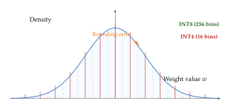
Remark 48.
The relationship between bit-width and accuracy is not linear. Empirically, going from FP16 to INT8 incurs accuracy loss for most models. Going from INT8 to INT4 incurs – loss without careful calibration (GPTQ/AWQ), but only – with it. Going below INT4 (e.g., INT2 or binary) typically requires quantization-aware training and incurs significant degradation on complex tasks.
Caution.
Outliers are the enemy of quantization. Quantization errors are not uniform across weights. Outlier weights, values far from the mean, cause disproportionate degradation because the quantization grid must span the full range, reducing resolution in the dense central region. A single outlier channel with magnitude the mean can halve the effective precision of the entire tensor. Always calibrate on representative data, and consider per-channel or per-group quantization to isolate outlier channels.
Key Idea.
The quantization toolkit. Post-training quantization (PTQ) methods like GPTQ and AWQ reduce model size by – with minimal accuracy loss, making LLMs deployable on consumer hardware. QLoRA extends this to fine-tuning, enabling personalisation of massive models on a single GPU. The key principle: not all weights are equal; protect the important ones (high-activation channels, outlier values) and compress the rest.
Trick #13 - Prune and Route
Two complementary ideas address the same question from opposite directions. Pruning asks: “Can we make a trained network smaller without losing accuracy?” Mixture of Experts (MoE) asks: “Can we make a network conditionally larger, using different subsets of parameters for different inputs?” Together, they represent the modern approach to parameter efficiency: use many parameters for capacity, but activate only a few for any given input.
Historical Note.
From brain damage to conditional computation. Pruning dates to LeCun et al.'s “Optimal Brain Damage” (1990), which removed weights based on second-order sensitivity. Han et al. (2015) [49] revived pruning for deep networks, achieving compression on AlexNet. Meanwhile, the Mixture of Experts concept was introduced by Jacobs et al. (1991) for shallow networks and scaled to deep learning by Shazeer et al. (2017) [50] with the Sparsely-Gated MoE layer. The convergence of these ideas in modern LLMs (Mixtral [51], DeepSeek-V3 [52], Switch Transformers [53]) has made conditional computation the dominant paradigm for scaling beyond a trillion parameters.
Magnitude pruning
The simplest pruning criterion: remove weights with the smallest magnitudes, on the assumption that small weights contribute least to the output.
Definition 54 (Magnitude Pruning).
Given trained weights , create a binary mask (Prune MASK) where is a threshold (typically chosen to achieve a target sparsity level , so that is the -th quantile of ). The pruned model uses weights . Two granularities:
Unstructured pruning: individual weights are zeroed, yielding sparse matrices.
Structured pruning: entire neurons, channels, or attention heads are removed, yielding smaller dense matrices.
Remark 49.
Unstructured pruning can reach + sparsity with accuracy loss on many tasks. However, exploiting unstructured sparsity requires hardware support for sparse matrix operations (e.g., NVIDIA's sparse tensor cores support structured sparsity at throughput). Structured pruning yields immediate speedups on standard hardware but typically tolerates less compression.
The Lottery Ticket Hypothesis
Pruning raises a deeper question: does a dense network need all those parameters, or does it contain a small subnetwork that could have learned just as well from the start?
Theorem 2 (Lottery Ticket Hypothesis).
(Frankle & Carbin, 2019 [54].) A randomly initialised dense network contains a subnetwork (the “winning ticket”) that, when trained in isolation with the same initialisation, achieves comparable accuracy to the full network in at most the same number of training iterations.
Formally, let be a dense network with random initialisation . There exists a mask with such that training for steps achieves test accuracy that of training for steps.
Algorithm 1 (Iterative Magnitude Pruning (IMP)).
The standard algorithm for finding lottery tickets:
Randomly initialise the network: .
Train to convergence: .
Prune of weights with smallest : .
Reset remaining weights to their original values: .
Repeat from step (b) with until the desired sparsity is reached.
Each round prunes of the surviving weights, so after rounds the network retains of its original parameters.
Remark 50.
Finding lottery tickets is computationally expensive: IMP requires full training for each pruning round. For a target sparsity of with per round, this requires rounds of full training. Research on efficient ticket-finding (e.g., early-bird tickets, one-shot pruning) aims to reduce this cost.
Mixture of Experts
Rather than making a network smaller, MoE makes it conditionally larger: the total parameter count grows, but each input activates only a small subset of “expert” sub-networks.
Definition 55 (Mixture of Experts Layer).
A Mixture of Experts layer with experts computes (MOE) where:
is the gating (or router) network,
is the -th expert (typically a feedforward network),
returns the indices of the largest entries of ,
is re-normalised over the selected experts.
Total parameters: . Active parameters per token: with .
A critical challenge in MoE training is expert collapse: the router learns to send most tokens to a few experts, leaving others untrained. The standard remedy is an auxiliary load-balancing loss.
Definition 56 (Load Balancing Loss).
The auxiliary load-balancing loss encourages uniform expert utilisation: (LOAD Balance) where is the fraction of tokens routed to expert in the current batch, is the average routing probability for expert (averaged over tokens), and is a small coefficient (typically ). This loss is minimised when for all (uniform routing).
Remark 51.
Switch Transformer [53]: uses (a single expert per token), the simplest possible routing. This minimises communication overhead in distributed settings and simplifies the load-balancing problem. Despite its simplicity, Switch Transformers achieve – speedups over dense models at the same compute budget.
Remark 52.
Mixtral [51]: uses experts selected from per MoE layer. Total parameters: 46.7B. Active parameters per token: 12.9B. This parameter efficiency enables Mixtral-8x7B to match or exceed LLaMA-2-70B on most benchmarks while using only 13B active parameters.
Remark 53.
DeepSeek-MoE [52]: introduces shared experts alongside routed experts. Some experts are always active (encoding shared knowledge common to all tokens), while others are conditionally selected. This hybrid design reduces the burden on the router and stabilises training.
Proposition 20 (MoE Capacity-Compute Trade-off).
For an MoE layer with experts of size and top- routing, the ratio of total parameters to active parameters is (MOE Ratio) This means a model can have times more parameters than a dense model of equal computational cost. For Mixtral (, ), ; for Switch (, ), . The larger , the greater the capacity per FLOP, but also the greater the memory footprint and communication overhead in distributed settings.
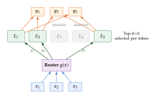
Trick #14 - Cache and Decode Faster
KV caching (Definition 16) and parallel attention+FFN blocks (Definition 21) were covered in the Transformer chapter. Here we turn to techniques that address the fundamental autoregressive bottleneck: generating one token at a time is inherently sequential.
Historical Note.
The autoregressive bottleneck. A language model generating a 100-token response must perform 100 serial forward passes, each waiting for the previous token. On modern hardware, each pass is memory-bandwidth bound (not compute-bound) during decoding, because the batch size is typically one token. The GPU's thousands of cores sit largely idle, waiting for data to arrive from memory. The quest: generate multiple tokens per step without changing the output distribution.
Speculative decoding
The key insight: use a small, fast model to draft several tokens, then verify them all at once with the large model. Because verification of tokens costs roughly the same as generating one (a single forward pass over positions), we get a speedup when most drafts are accepted.
Definition 57 (Speculative Decoding).
Let be a small, fast draft model and be the large target model. Speculative decoding [55] proceeds as follows:
Draft: generates candidate tokens autoregressively.
Verify: computes logits for all positions in a single forward pass (exploiting KV caching and parallel computation).
Accept/Reject: for each position , accept with probability (SPEC Accept)
If is rejected, resample from the adjusted distribution (SPEC Resample) and discard all subsequent draft tokens.
The crucial property of speculative decoding is that it produces exactly the same output distribution as the target model.
Proposition 21 (Speculative Decoding Correctness).
The output distribution of speculative decoding is identical to that of the target model .
Proof.
This is a Metropolis–Hastings-style rejection sampling scheme. For any token at position , the marginal probability under speculative decoding is: Case 1: . The acceptance probability is , contributing . The resampling contributes the remaining (from the adjusted distribution). Total: .
Case 2: . The acceptance probability is , contributing . The resampling assigns zero probability to (since ). Total: .
In both cases, .
Proposition 22 (Expected Speedup).
If the per-token acceptance rate is (i.e., each drafted token is accepted with probability , independently), the expected number of accepted tokens per verification step is (SPEC Expected) where is the draft length.
Proof.
Let be the number of accepted tokens (including the one generated at the rejection point). We have for , and the last position always generates a valid token (either accepted or resampled). Thus: The effective speedup over standard decoding is approximately where and are the per-token costs of the draft and target models, respectively.
Remark 54.
With and : accepted tokens per verification step. If the draft model costs of the target model, the speedup is .
Medusa decoding
Speculative decoding requires a separate draft model. Medusa eliminates this requirement by adding prediction heads directly to the target model.
Definition 58 (Medusa Decoding).
Medusa [56] adds extra prediction heads to the model, each predicting the -th future token: (Medusa) where is the hidden state at position and is the -th head's projection. At each step:
Generate candidate tokens: one from the original head (position ) and from the Medusa heads (positions ).
Construct a candidate tree from the top- predictions of each head.
Verify all candidates with a single forward pass using tree attention: attention masks are structured so that each candidate attends only to its ancestors in the tree.
Accept the longest prefix that matches the target model's predictions.
No separate draft model is needed; the target model does both drafting and verification.
Weight tying
A simple but effective trick that reduces parameters and improves performance simultaneously.
Definition 59 (Weight Tying).
Set the output projection matrix equal to the transpose of the input embedding matrix [57]: (TIED Embed) Parameter savings: fewer parameters, where is the vocabulary size. For and , this saves approximately 200M parameters ( MB in FP16).
Remark 55.
Weight tying is essentially free: it saves memory and often improves performance by providing implicit regularisation. The intuition is that the input embedding learns to map tokens into a semantic space, and the output projection should map back to the same space, so sharing weights enforces this consistency. Nearly all modern language models use weight tying.
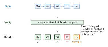
Key Idea.
Lossless speedup. Speculative decoding is the only inference trick that provides a strict speedup with zero quality loss: the output distribution is mathematically identical to that of the target model. Every other speed optimisation (quantization, pruning, distillation) trades quality for speed; speculative decoding trades draft model compute for target model parallelism.
Trick #15 - Combine Tricks Synergistically
No trick works in isolation. The power of the techniques covered in Trick #1 - Initialize Wisely–Trick #14 - Cache and Decode Faster lies not in any single trick but in their synergistic combination. A modern large language model is a carefully composed symphony of tricks working in concert, each addressing a specific failure mode while remaining compatible with the others.
Key Idea.
The meta-trick. The modern LLM is not a single trick but a carefully composed symphony of tricks working together. The art of deep learning engineering is knowing which tricks to combine, in what order, and how they interact. A poor combination (e.g., BatchNorm + Pre-norm + ReZero) is redundant; a good combination (e.g., RMSNorm + SwiGLU + RoPE + GQA + Flash Attention) is greater than the sum of its parts.
Model recipe analysis
Table 5 shows which tricks are used by several prominent LLMs. The convergence on a common “recipe” is striking: nearly all models use pre-norm RMSNorm, SwiGLU activations, RoPE positional encoding, and some form of efficient attention.
| Trick | LLaMA-2 | Qwen-2.5 | DeepSeek-V3 | Mistral | GPT-4 |
| Init | He | He | He | He | He |
| Gating | SwiGLU | SwiGLU | SwiGLU | SwiGLU | (unknown) |
| Norm | RMSNorm | RMSNorm | RMSNorm | RMSNorm | LayerNorm |
| (pre) | (pre) | (pre) | (pre) | (pre) | |
| Skip | Residual | Residual | mHC | Residual | Residual |
| Activation | SiLU | SiLU | SiLU | SiLU | (unknown) |
| Position | RoPE | RoPE | RoPE | RoPE | (unknown) |
| Attention | GQA | GQA | MLA | GQA | (unknown) |
| Regularise | - | - | DropPath | - | (unknown) |
| LR | Cosine | Cosine | WSD | Cosine | Cosine |
| Precision | BF16 | BF16 | BF16+FP8 | BF16 | (unknown) |
| MoE | No | No | Yes | No | Yes |
| GPT-4 architecture is not publicly disclosed; entries are community estimates. | |||||
| Mixtral uses MoE; base Mistral does not. | |||||
Interaction effects
Understanding why certain tricks compose well is as important as knowing which ones to use.
The LLaMA recipe: RMSNorm + SwiGLU + RoPE.
These three tricks compose synergistically because each operates on a different aspect of the architecture. RMSNorm is computationally cheap (no mean subtraction, no bias) and stabilises training without introducing extra parameters. SwiGLU adds expressiveness to the FFN block via learnable gating. RoPE handles position without added parameters and naturally supports length extrapolation. None interferes with the others: RMSNorm normalises activations before SwiGLU processes them, and RoPE acts only on attention queries and keys.
Pre-norm + ReZero: redundant?
Pre-norm (Trick #3 - Normalise Everything) already ensures well-behaved gradients at initialisation by normalising inputs to each sub-layer. ReZero's learnable scalar (initialised at zero) addresses the same problem from a different angle. Combining both is redundant: if at init, the normalisation has nothing to normalise. In practice, one should choose either pre-norm (the standard) or ReZero (simpler but less common), not both.
MoE + quantization challenges.
Different experts may have different weight distributions, making a single quantization scale suboptimal. Per-expert quantization is necessary but increases the number of quantization parameters. Moreover, expert-level load imbalance means that heavily used experts accumulate more gradient noise, potentially requiring expert-specific precision settings.
Gated Attention + Flash Attention.
The element-wise gate in gated attention (Trick #2 - Make It Gated) is applied after the attention computation, so it adds minimal overhead to Flash Attention's IO-optimal algorithm. The two compose cleanly.
Open research directions
Automatic trick discovery. Can neural architecture search (NAS) discover new tricks? Most NAS work searches over macro-architecture (layer counts, widths); searching over micro-architecture (normalisation placement, gating variants, skip-connection topology) is largely unexplored.
Theoretical understanding. Why do these tricks compose well? Information-theoretic analyses of individual tricks exist (e.g., residual connections preserve mutual information with the input), but a unified theory of trick composition is lacking.
Scaling laws for tricks. Do tricks help more or less at scale? Preliminary evidence suggests that some tricks (e.g., careful initialisation) matter less at scale (large models are more robust to initialisation), while others (e.g., MoE, mixed precision) matter more (they enable training at scales that would otherwise be infeasible).
Hardware-aware trick design. As hardware evolves (e.g., AMD MI300, Google TPUs, Cerebras wafer-scale), the optimal trick recipe changes. Tricks optimised for NVIDIA A100s may be suboptimal on TPUs (which have different memory hierarchies and matrix unit sizes).
Biological analogues. Many tricks have biological counterparts: gating in neurons (ion channel modulation), normalisation in neural populations (divisive normalisation), pruning during development (synaptic pruning in adolescence). Can biological insights suggest new tricks?
Insight.
The next breakthrough. The next breakthrough may not be a new trick but a deeper understanding of why existing tricks work together. A principled theory of trick composition would enable automatic recipe design for new architectures, new hardware, and new tasks, replacing the current approach of manual experimentation guided by intuition and precedent.
Historical Timeline
The techniques covered in this chapter emerged over four decades of research. Figure 16 traces their evolution, from the foundational ideas of the 1980s to the efficiency innovations of the 2020s.
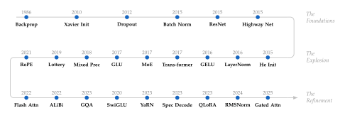
Narrative: four eras of tricks
1986–2010: The dark ages.
Training deep networks was black magic. Backpropagation existed (Rumelhart et al., 1986), but networks deeper than 2–3 layers routinely failed to train. Initialisation was ad hoc (often uniform random), normalisation was non-existent, and the gradient dynamics of deep networks were poorly understood. The few practitioners who achieved results relied on extensive manual tuning and domain-specific architectures.
2010–2015: The foundations.
Three foundational tricks made deep training possible. Xavier initialisation (2010) showed that variance-preserving init enables gradient flow through many layers. Dropout (2012) provided the first effective regulariser for deep networks. Batch normalisation and residual connections (both 2015) made it possible to train networks with layers reliably. These tricks transformed deep learning from an art into a science.
2015–2020: The explosion.
The Transformer architecture (2017) [24] combined several tricks (residual connections, layer normalisation, scaled dot-product attention) into a unified framework that scaled to billions of parameters. This era saw rapid innovation: GELU activations, GLU variants, RoPE, mixed-precision training, and the Lottery Ticket Hypothesis. By 2020, the basic recipe for billion-parameter language models was established.
2020–2025: The refinement.
The challenge shifted from “can we train large models?” to “can we train and deploy them efficiently?” Flash Attention made attention IO-optimal. Grouped-query attention reduced KV cache memory. SwiGLU replaced standard FFNs. Quantization (GPTQ, AWQ, QLoRA) made LLMs runnable on consumer hardware. Speculative decoding achieved lossless speedup. RMSNorm replaced LayerNorm. Each refinement was small individually; together, they enabled the deployment of models that would have been impractical in 2020.
Historical Note.
A coherent theory of deep network design. Looking back, each trick solved a specific failure mode: Xavier init solved vanishing activations; residual connections solved vanishing gradients; normalisation solved internal covariate shift; gating solved expressiveness bottlenecks; efficient attention solved the quadratic complexity wall. Together, they form a coherent, if empirically discovered, theory of deep network design: preserve signal flow, stabilise statistics, gate information, and minimise computational waste.
Exercises
The following exercises cover all 15 tricks presented in this chapter, ranging from straightforward derivations to open-ended design problems.
Exercise 1 (Xavier Initialisation Derivation).
Consider a linear layer with , where and are i.i.d. with mean and variance .
Show that .
Derive the condition for forward-pass variance preservation ().
Repeat the analysis for the backward pass (gradient propagation through ) to obtain .
Show that the harmonic mean balances both forward and backward passes.
Exercise 2 (He Initialisation for ReLU).
Let . We wish to compute .
Compute and show that the result is .
Using the result from (a) and the analysis of Exercise 1, derive the He initialisation variance .
Exercise 3 (GLU Gradient Flow).
Compare gradient magnitude through a standard FFN and a GLU .
Compute for the standard FFN. Express it in terms of and .
Compute for the GLU. Use the product rule for the Hadamard product to obtain two terms.
Explain why the GLU gradient has a direct linear path (through ) that survives even when the sigmoid saturates. Contrast this with the standard FFN, where saturation kills the gradient entirely.
Exercise 4 (Gated Attention Expressiveness).
Show that the standard attention output for query lies in , the convex hull of the value vectors (since attention weights sum to 1 and are non-negative).
Show that the gated attention output can lie outside this convex hull when has entries or entries with different signs.
Give a concrete 2D example: let , , attention weights , and gate . Compute the gated output and verify it is not in .
Exercise 5 (GroupNorm as Interpolation).
Let GroupNorm with groups operate on a feature map with channels. Show that GroupNorm reduces to:
LayerNorm when (all channels in a single group).
InstanceNorm when (each channel is its own group).
In each case, explicitly write the set of elements over which the mean and variance are computed.
Exercise 6 (DeepNorm Scaling Derivation).
In a transformer with sub-layers using DeepNorm: , where is initialised at scale (i.e., ).
Show that after layers with the above recurrence, the expected output variance (before LN) is .
Choose and as functions of so that this variance is .
Verify that and satisfies this condition.
Exercise 7 (Pre-Norm vs Post-Norm Gradient).
Compare gradient flow for residual layers.
Post-norm: . Show that involves applications of the LayerNorm Jacobian , which can amplify or attenuate gradients.
Pre-norm: . Show that , so the gradient has a direct path through the identity, ensuring it never vanishes regardless of depth.
Exercise 8 (DenseNet Parameter Count).
A DenseNet block with layers and growth rate (each layer produces feature maps).
Compute the input dimension to the -th layer, given that it receives feature maps from all previous layers: , where is the initial channel count.
Count the total parameters for the block, assuming each layer is a convolution: .
Compare with a ResNet of the same depth with constant width . Which uses fewer parameters, and by how much?
Exercise 9 (mHC Doubly Stochastic Properties).
Show that the doubly stochastic matrices form a line segment: .
Show that the product of two doubly stochastic matrices is doubly stochastic.
Show that (the set of doubly stochastic matrices) has exactly 6 vertices, namely the permutation matrices (Birkhoff's theorem).
Show that the spectral norm of any doubly stochastic matrix is at most . Hint: the all-ones vector is an eigenvector with eigenvalue , and all eigenvalues have modulus .
Exercise 10 (Dying ReLU Probability).
Under He initialisation with and :
Compute the probability that for a random input . Hint: what is the distribution of ?
After one gradient step with learning rate on a single example , compute the probability that the neuron remains dead. Discuss how this depends on and the loss function.
Exercise 11 (SELU Fixed Point).
Let , with and .
Compute for . Split the integral at .
Compute for .
Verify numerically that and , confirming that is a fixed point of the mean-variance map.
Exercise 12 (ALiBi vs RoPE Decay).
For a head with ALiBi slope and head dimension :
Compute the ALiBi attention weight modification: . What fraction of the unmodified weight remains at distance ?
For RoPE, show that the attention decay with distance depends on the alignment of query and key vectors, not just the distance. Write out the inner product and identify the distance-dependent and content-dependent factors.
At distance , compare the ALiBi relative weight with a typical RoPE decay. Which mechanism provides a harder position cutoff?
Exercise 13 (NTK Scaling Derivation).
RoPE uses frequencies with . To extend from context length to :
Show that naïve position interpolation (dividing positions by ) reduces all frequencies by a factor of , including high-frequency components that were well within the training range.
Explain why high-frequency components (small , large ) need less interpolation than low-frequency ones: they already have many cycles within .
Derive the NTK-aware scaling formula: . Show that this interpolates the lowest-frequency component by factor while leaving the highest-frequency component nearly unchanged.
Exercise 14 (YaRN Frequency Zones).
For , , (scale ):
Compute the wavelength for .
With ramp parameters and , classify each frequency dimension into low/medium/high frequency zones.
Compute the interpolation factor for each dimension: (no change) for high frequency, (full interpolation) for low frequency, and linear ramp for medium frequency.
Exercise 15 (Sparse Attention Complexity).
Consider combined local (window ) + strided (stride ) attention on sequence length .
Count the number of positions each token attends to: .
Show that the total complexity (over all tokens) is .
Choose and show this gives total complexity, subquadratic in .
Exercise 16 (Ring Attention Communication).
For devices, sequence length , model dimension , and attention heads with dimension :
Compute the size of KV blocks transmitted per round: each device sends , so the message size is .
Compute the total communication volume for rounds.
Compare with all-to-all communication (where every device sends its KV to every other device). Under what conditions is ring attention preferable?
Exercise 17 (Dropout as Ensemble).
Consider a -layer network with neurons per layer and dropout rate .
Enumerate all possible sub-networks obtained by dropping neurons. How many are there? (Count the number of binary masks over 4 neurons: .)
For a specific input , compute the ensemble average for a simple linear network .
Show that inference with all neurons active and weights scaled by approximates the ensemble average.
Exercise 18 (Label Smoothing Calibration).
With smoothing parameter and classes:
Compute the target distribution: the correct class receives probability ; each incorrect class receives .
At the optimal cross-entropy solution, the logit difference between the correct class and any incorrect class is bounded. Show that the maximum logit gap is .
Compare with hard labels (), where the optimal logit for the correct class is . Explain why bounded logits improve calibration.
Exercise 19 (Mixup as Vicinal Risk).
Define the vicinal distribution for Mixup: given two training pairs and , the virtual example is with .
Show that when (i.e., ).
Show that as , with probability 1 (the Beta distribution concentrates at its mean), making Mixup a simple average of two examples.
Exercise 20 (Cosine vs Step Decay).
Compare the total “learning signal” (integral of LR over time) for cosine annealing and step decay (divide by 10 at and of training). Let be the peak learning rate and the total training steps.
Compute , where .
Compute , where for , for , and for .
Which schedule provides more total gradient signal? Compute the ratio.
Exercise 21 (WSD Schedule Properties).
The Warmup-Stable-Decay (WSD) schedule maintains a constant learning rate during the “stable” phase, then decays.
Show that WSD is “anytime optimal”: at any point during the stable phase, branching into a cosine decay reaching produces a valid schedule. Why is this useful for long training runs where the total duration is uncertain?
Compare the total learning signal for WSD (with stable phase ) vs. cosine with the same .
When would WSD be preferred over cosine? Hint: consider continual pretraining scenarios where new data arrives during training.
Exercise 22 (BF16 vs FP16 Range).
Compute the maximum representable value for FP16 (1 sign, 5 exponent, 10 mantissa bits) and BF16 (1 sign, 8 exponent, 7 mantissa bits).
Compute the minimum positive normal value for each format.
For a gradient of magnitude , determine whether it underflows (falls below the minimum normal) in FP16 and BF16.
Explain why BF16 is preferred for training despite having lower precision (7 vs. 10 mantissa bits): the larger exponent range ( decades vs. decades) prevents overflow and underflow during training.
Exercise 23 (Loss Scaling Factor).
What is the smallest positive normal FP16 number? Show that it is .
If typical gradients have magnitude (below the FP16 normal range), compute the minimum loss scale factor needed to prevent underflow: .
If the loss scale is , compute the maximum gradient magnitude before overflow: . Is this a concern in practice?
Exercise 24 (Distillation Temperature).
Given teacher logits :
Compute for . Observe how the distribution flattens as increases.
Verify that as , the distribution approaches (uniform over 3 classes).
For the KL divergence term in the distillation loss, compute at for each temperature . Show that this gradient is zero (as expected, since the student matches the teacher).
Exercise 25 (GPTQ Error Analysis).
For a weight matrix and INT4 symmetric quantization with :
Compute the scale factor .
Quantize each weight: . Compute the quantized values and the element-wise quantization error .
Assume the Hessian (identity) for simplicity. Apply the GPTQ correction: after quantizing column 1, update column 2 as . Show that this reduces the reconstruction error .
Exercise 26 (Lottery Ticket Sparsity).
Starting with a network of parameters, IMP prunes of surviving parameters each round.
After rounds, how many parameters remain? Express as .
How many rounds are needed to reach of the original parameters? Solve .
If each round requires full retraining (cost per round), what is the total compute cost to find the -sparse ticket? Compare with the cost of training the full network once.
Exercise 27 (MoE Load Balancing).
With experts and a batch of tokens:
Show that the auxiliary loss is minimised when for all . Hint: use the AM-GM inequality or Lagrange multipliers, subject to and .
Compute when one expert receives of tokens (i.e., , ) and .
Compute the gradient and explain how it pushes the router towards uniform routing.
Exercise 28 (Speculative Decoding Speedup).
With acceptance rate , draft length , and cost ratio :
Compute . Show that .
Compute the cost per verification step: .
Compute the effective speedup: .
Plot the speedup as a function of for . At what acceptance rate does speculative decoding become slower than standard decoding?
Exercise 29 (Trick Interactions).
Explain why Fixup initialisation + BatchNorm is redundant: both address the problem of maintaining activation scale through deep residual networks. If BatchNorm is present, what purpose does Fixup's careful scaling serve?
Explain why DropPath + ReZero could interact poorly at initialisation. With ReZero's initially, each residual branch contributes nothing; DropPath then randomly zeros out a branch that already contributes nothing. What happens to the gradient signal?
Design a combination of 5 tricks for a new 1B-parameter vision model (ViT-style). For each trick, state: (i) the specific variant, (ii) why it is appropriate for this scale and modality, and (iii) how it interacts with the other chosen tricks.
Exercise 30 (Design a Novel Trick).
Propose a new gating mechanism for the FFN layer that differs from GLU, SwiGLU, and GEGLU. Suggestion: consider multiplicative interactions involving more than two branches, or adaptive gating conditioned on the layer index or a running statistics estimate.
Write the mathematical formulation of your proposed mechanism: .
Analyse the gradient flow through your mechanism. Specifically, compute and identify whether a direct linear path exists (as in GLU).
Discuss potential advantages and disadvantages compared to SwiGLU. Consider: parameter count, computational cost, gradient flow properties, and ease of implementation.
0.60.5pt
The exercises above span the full range of tricks covered in this chapter. Exercises 1–9 test foundational understanding of individual tricks; Exercises 10–16 develop quantitative analysis skills; Exercises 17–23 connect tricks to practical engineering decisions; Exercises 24–28 require numerical computation and verification; and Exercises 29–30 develop design intuition by asking you to analyse interactions and propose new ideas. Solutions to selected exercises (marked with ) are available in Appendix B.
References
-
Efficient BackProp
BibTeX
@incollection{lecun1998efficient, title={Efficient {BackProp}}, author={LeCun, Yann and Bottou, L\'{e}on and Orr, Genevieve B. and M\"{u}ller, Klaus-Robert}, booktitle={Neural Networks: Tricks of the Trade}, publisher={Springer}, pages={9--50}, year={1998} }Book chapter
-
Understanding the Difficulty of Training Deep Feedforward Neural Networks
BibTeX
@inproceedings{glorot2010understanding, title={Understanding the Difficulty of Training Deep Feedforward Neural Networks}, author={Glorot, Xavier and Bengio, Yoshua}, booktitle={International Conference on Artificial Intelligence and Statistics (AISTATS)}, pages={249--256}, year={2010} }Conference paper
-
Delving Deep into Rectifiers: Surpassing Human-Level Performance on ImageNet Classification
BibTeX
@inproceedings{he2015delving, title={Delving Deep into Rectifiers: Surpassing Human-Level Performance on {ImageNet} Classification}, author={He, Kaiming and Zhang, Xiangyu and Ren, Shaoqing and Sun, Jian}, booktitle={IEEE International Conference on Computer Vision (ICCV)}, pages={1026--1034}, year={2015} }Conference paper
-
Tensor Programs V: Tuning Large Neural Networks via Zero-Shot Hyperparameter Transfer
BibTeX
@misc{yang2022tensor, title={Tensor Programs {V}: Tuning Large Neural Networks via Zero-Shot Hyperparameter Transfer}, author={Yang, Greg and Hu, Edward J. and Babuschkin, Igor and Sidor, Szymon and Liu, Xiaodong and Farhi, David and Ryder, Nick and Pachocki, Jakub and Chen, Weizhu and Gao, Jianfeng}, year={2022}, eprint={2203.03466}, archiveprefix={arXiv}, primaryclass={cs.LG} }Reference
-
Exact Solutions to the Nonlinear Dynamics of Learning in Deep Linear Neural Networks
BibTeX
@inproceedings{saxe2013exact, title={Exact Solutions to the Nonlinear Dynamics of Learning in Deep Linear Neural Networks}, author={Saxe, Andrew M. and McClelland, James L. and Ganguli, Surya}, booktitle={International Conference on Learning Representations (ICLR)}, year={2014} }Conference paper
-
All You Need is a Good Init
BibTeX
@inproceedings{mishkin2016lsuv, title={All You Need is a Good Init}, author={Mishkin, Dmytro and Matas, Jiri}, booktitle={International Conference on Learning Representations (ICLR)}, year={2016} }Conference paper
-
Fixup Initialization: Residual Learning Without Normalization
BibTeX
@inproceedings{zhang2019fixup, title={Fixup Initialization: Residual Learning Without Normalization}, author={Zhang, Hongyi and Dauphin, Yann N. and Ma, Tengyu}, booktitle={International Conference on Learning Representations (ICLR)}, year={2019} }Conference paper
-
Long Short-Term Memory
BibTeX
@article{hochreiter1997long, title={Long Short-Term Memory}, author={Hochreiter, Sepp and Schmidhuber, J{\"u}rgen}, journal={Neural Computation}, volume={9}, number={8}, pages={1735--1780}, year={1997} }Journal article
-
Learning Phrase Representations using RNN Encoder--Decoder for Statistical Machine Translation
BibTeX
@inproceedings{cho2014learning, title={Learning Phrase Representations using {RNN} Encoder--Decoder for Statistical Machine Translation}, author={Cho, Kyunghyun and van Merrienboer, Bart and Gulcehre, Caglar and Bahdanau, Dzmitry and Bougares, Fethi and Schwenk, Holger and Bengio, Yoshua}, booktitle={Proceedings of the 2014 Conference on Empirical Methods in Natural Language Processing (EMNLP)}, pages={1724--1734}, year={2014} }Conference paper
-
Highway Networks
BibTeX
@misc{srivastava2015highway, title={Highway Networks}, author={Srivastava, Rupesh Kumar and Greff, Klaus and Schmidhuber, J\"{u}rgen}, year={2015}, eprint={1505.00387}, archiveprefix={arXiv}, primaryclass={cs.LG} }Reference
-
Language Modeling with Gated Convolutional Networks
BibTeX
@inproceedings{dauphin2017language, title={Language Modeling with Gated Convolutional Networks}, author={Dauphin, Yann N. and Fan, Angela and Auli, Michael and Grangier, David}, booktitle={International Conference on Machine Learning (ICML)}, pages={933--941}, year={2017} }Conference paper
-
GLU Variants Improve Transformer
BibTeX
@article{shazeer2020glu, title={{GLU} Variants Improve Transformer}, author={Shazeer, Noam}, journal={arXiv preprint arXiv:2002.05202}, year={2020} }Journal article
-
Gated Attention for Large Language Models
BibTeX
@inproceedings{qiu2025gated, title={Gated Attention for Large Language Models}, author={Qiu, Zihan and Wang, Zekun and Zheng, Bo and Huang, Zeyu and Wen, Kaiyue and Yang, Songlin and Men, Rui and Yu, Le and Huang, Fei and Huang, Suozhi and Liu, Dayiheng and Zhou, Jingren and Lin, Junyang}, booktitle={Advances in Neural Information Processing Systems}, volume={38}, year={2025} }Conference paper
-
Highway and Residual Networks Learn Unrolled Iterative Estimation
BibTeX
@inproceedings{greff2017highway, title={Highway and Residual Networks Learn Unrolled Iterative Estimation}, author={Greff, Klaus and Srivastava, Rupesh Kumar and Schmidhuber, J\"{u}rgen}, booktitle={International Conference on Learning Representations (ICLR)}, year={2017} }Conference paper
-
Batch Normalization: Accelerating Deep Network Training by Reducing Internal Covariate Shift
BibTeX
@inproceedings{ioffe2015batch, title={Batch Normalization: Accelerating Deep Network Training by Reducing Internal Covariate Shift}, author={Ioffe, Sergey and Szegedy, Christian}, booktitle={International Conference on Machine Learning (ICML)}, pages={448--456}, year={2015} }Conference paper
-
How Does Batch Normalization Help Optimization?
BibTeX
@inproceedings{santurkar2018does, title={How Does Batch Normalization Help Optimization?}, author={Santurkar, Shibani and Tsipras, Dimitris and Ilyas, Andrew and Madry, Aleksander}, booktitle={Advances in Neural Information Processing Systems (NeurIPS)}, year={2018} }Conference paper
-
DeepNet: Scaling Transformers to 1,000 Layers
BibTeX
@misc{wang2022deepnet, title={{DeepNet}: Scaling Transformers to 1,000 Layers}, author={Wang, Hongyu and Ma, Shuming and Dong, Li and Huang, Shaohan and Zhang, Dongdong and Wei, Furu}, year={2022}, eprint={2203.00555}, archiveprefix={arXiv}, primaryclass={cs.LG} }Reference
-
Deep Residual Learning for Image Recognition
BibTeX
@inproceedings{he2016deep, title={Deep Residual Learning for Image Recognition}, author={He, Kaiming and Zhang, Xiangyu and Ren, Shaoqing and Sun, Jian}, booktitle={IEEE Conference on Computer Vision and Pattern Recognition (CVPR)}, pages={770--778}, year={2016} }Conference paper
-
Fast and Accurate Deep Network Learning by Exponential Linear Units (ELUs)
BibTeX
@inproceedings{clevert2015fast, title={Fast and Accurate Deep Network Learning by Exponential Linear Units ({ELUs})}, author={Clevert, Djork-Arn\'{e} and Unterthiner, Thomas and Hochreiter, Sepp}, booktitle={International Conference on Learning Representations (ICLR)}, year={2016} }Conference paper
-
Self-Normalizing Neural Networks
BibTeX
@inproceedings{klambauer2017self, title={Self-Normalizing Neural Networks}, author={Klambauer, G\"{u}nter and Unterthiner, Thomas and Mayr, Andreas and Hochreiter, Sepp}, booktitle={Advances in Neural Information Processing Systems (NeurIPS)}, year={2017} }Conference paper
-
Gaussian Error Linear Units (GELUs)
BibTeX
@misc{hendrycks2016gaussian, title={Gaussian Error Linear Units ({GELUs})}, author={Hendrycks, Dan and Gimpel, Kevin}, year={2016}, eprint={1606.08415}, archiveprefix={arXiv}, primaryclass={cs.LG} }Reference
-
Searching for Activation Functions
BibTeX
@misc{ramachandran2017searching, title={Searching for Activation Functions}, author={Ramachandran, Prajit and Zoph, Barret and Le, Quoc V.}, year={2017}, eprint={1710.05941}, archiveprefix={arXiv}, primaryclass={cs.NE} }Reference
-
Mish: A Self Regularized Non-Monotonic Activation Function
BibTeX
@misc{misra2019mish, title={Mish: A Self Regularized Non-Monotonic Activation Function}, author={Misra, Diganta}, year={2019}, eprint={1908.08681}, archiveprefix={arXiv}, primaryclass={cs.LG} }Reference
-
Attention is all you need
BibTeX
@inproceedings{vaswani2017attention, title={Attention is all you need}, author={Vaswani, Ashish and Shazeer, Noam and Parmar, Niki and Uszkoreit, Jakob and Jones, Llion and Gomez, Aidan N and Kaiser, {\L}ukasz and Polosukhin, Illia}, booktitle={Advances in neural information processing systems}, pages={5998--6008}, year={2017} }Conference paper
-
RoFormer: Enhanced Transformer with Rotary Position Embedding
BibTeX
@article{su2024roformer, title={{RoFormer}: Enhanced Transformer with Rotary Position Embedding}, author={Su, Jianlin and Ahmed, Murtadha and Lu, Yu and Pan, Shengfeng and Bo, Wen and Liu, Yunfeng}, journal={Neurocomputing}, volume={568}, pages={127063}, year={2024}, publisher={Elsevier} }Journal article
-
Train Short, Test Long: Attention with Linear Biases Enables Input Length Extrapolation
BibTeX
@inproceedings{press2022alibi, title={Train Short, Test Long: Attention with Linear Biases Enables Input Length Extrapolation}, author={Press, Ofir and Smith, Noah A. and Lewis, Mike}, booktitle={International Conference on Learning Representations (ICLR)}, year={2022} }Conference paper
-
YaRN: Efficient Context Window Extension of Large Language Models
BibTeX
@misc{peng2023yarn, title={{YaRN}: Efficient Context Window Extension of Large Language Models}, author={Peng, Bowen and Quesnelle, Jeffrey and Fan, Honglu and Shippole, Enrico}, year={2023}, eprint={2309.00071}, archiveprefix={arXiv}, primaryclass={cs.CL} }Reference
-
NTK-Aware Scaled RoPE Allows LLaMA Models to Have Extended Context
BibTeX
@misc{ntk2023rope, title={{NTK}-Aware Scaled {RoPE} Allows {LLaMA} Models to Have Extended Context}, author={bloc97}, year={2023}, howpublished={Reddit post and community discovery}, note={Community-discovered method for extending RoPE context length via Neural Tangent Kernel-aware interpolation} }Reference
-
Mistral 7B
BibTeX
@article{jiang2023mistral, title={{Mistral 7B}}, author={Jiang, Albert Q. and Sablayrolles, Alexandre and Mensch, Arthur and Bamford, Chris and Chaplot, Devendra Singh and de las Casas, Diego and Bressand, Florian and Lengyel, Gianna and Lample, Guillaume and Saulnier, Lucile and others}, journal={arXiv preprint arXiv:2310.06825}, year={2023} }Journal article
-
Longformer: The Long-Document Transformer
BibTeX
@article{beltagy2020longformer, title={Longformer: The Long-Document Transformer}, author={Beltagy, Iz and Peters, Matthew E. and Cohan, Arman}, journal={arXiv preprint arXiv:2004.05150}, year={2020} }Journal article
-
Transformers are RNNs: Fast Autoregressive Transformers with Linear Attention
BibTeX
@inproceedings{katharopoulos2020transformers, title={Transformers are {RNNs}: Fast Autoregressive Transformers with Linear Attention}, author={Katharopoulos, Angelos and Vyas, Apoorv and Pappas, Nikolaos and Fleuret, Fran\c{c}ois}, booktitle={International Conference on Machine Learning (ICML)}, pages={5156--5165}, year={2020} }Conference paper
-
Dropout as a Bayesian Approximation: Representing Model Uncertainty in Deep Learning
BibTeX
@inproceedings{gal2016dropout, title={Dropout as a {B}ayesian Approximation: Representing Model Uncertainty in Deep Learning}, author={Gal, Yarin and Ghahramani, Zoubin}, booktitle={Proceedings of the International Conference on Machine Learning (ICML)}, pages={1050--1059}, year={2016} }Conference paper
-
Rethinking the Inception Architecture for Computer Vision
BibTeX
@inproceedings{szegedy2016rethinking, title={Rethinking the Inception Architecture for Computer Vision}, author={Szegedy, Christian and Vanhoucke, Vincent and Ioffe, Sergey and Shlens, Jon and Wojna, Zbigniew}, booktitle={IEEE Conference on Computer Vision and Pattern Recognition (CVPR)}, pages={2818--2826}, year={2016} }Conference paper
-
mixup: Beyond Empirical Risk Minimization
BibTeX
@inproceedings{zhang2018mixup, title={mixup: Beyond Empirical Risk Minimization}, author={Zhang, Hongyi and Cisse, Moustapha and Dauphin, Yann N. and Lopez-Paz, David}, booktitle={International Conference on Learning Representations (ICLR)}, year={2018} }Conference paper
-
CutMix: Regularization Strategy to Train Strong Classifiers with Localizable Features
BibTeX
@inproceedings{yun2019cutmix, title={{CutMix}: Regularization Strategy to Train Strong Classifiers with Localizable Features}, author={Yun, Sangdoo and Han, Dongyoon and Oh, Seong Joon and Chun, Sanghyuk and Choe, Junsuk and Yoo, Youngjoon}, booktitle={IEEE International Conference on Computer Vision (ICCV)}, pages={6023--6032}, year={2019} }Conference paper
-
R-Drop: Regularized Dropout for Neural Networks
BibTeX
@inproceedings{liang2021rdrop, title={{R-Drop}: Regularized Dropout for Neural Networks}, author={Liang, Xiaobo and Wu, Lijun and Li, Juntao and Wang, Yue and Meng, Qi and Qin, Tao and Chen, Wei and Zhang, Min and Liu, Tie-Yan}, booktitle={Advances in Neural Information Processing Systems (NeurIPS)}, year={2021} }Conference paper
-
SGDR: Stochastic Gradient Descent with Warm Restarts
BibTeX
@inproceedings{loshchilov2017sgdr, title={{SGDR}: Stochastic Gradient Descent with Warm Restarts}, author={Loshchilov, Ilya and Hutter, Frank}, booktitle={International Conference on Learning Representations (ICLR)}, year={2017} }Conference paper
-
Cyclical Learning Rates for Training Neural Networks
BibTeX
@inproceedings{smith2017cyclical, title={Cyclical Learning Rates for Training Neural Networks}, author={Smith, Leslie N.}, booktitle={IEEE Winter Conference on Applications of Computer Vision (WACV)}, pages={464--472}, year={2017} }Conference paper
-
Accurate, Large Minibatch SGD: Training ImageNet in 1 Hour
BibTeX
@misc{goyal2017accurate, title={Accurate, Large Minibatch {SGD}: Training {ImageNet} in 1 Hour}, author={Goyal, Priya and Doll\'{a}r, Piotr and Girshick, Ross and Noordhuis, Pieter and Wesolowski, Lukasz and Kyrola, Aapo and Tulloch, Andrew and Jia, Yangqing and He, Kaiming}, year={2017}, eprint={1706.02677}, archiveprefix={arXiv}, primaryclass={cs.CV} }Reference
-
Mixed Precision Training
BibTeX
@inproceedings{micikevicius2018mixed, title={Mixed Precision Training}, author={Micikevicius, Paulius and Narang, Sharan and Alben, Jonah and Diamos, Gregory and Elsen, Erich and Garcia, David and Ginsburg, Boris and Houston, Michael and Kuchaiev, Oleksii and Venkatesh, Ganesh and Wu, Hao}, booktitle={International Conference on Learning Representations (ICLR)}, year={2018} }Conference paper
-
Knowledge Distillation: A Survey
BibTeX
@article{gou2021knowledge, title={Knowledge Distillation: A Survey}, author={Gou, Jianping and Yu, Baosheng and Maybank, Stephen J. and Tao, Dacheng}, journal={International Journal of Computer Vision}, volume={129}, number={6}, pages={1789--1819}, year={2021} }Journal article
-
Distilling the Knowledge in a Neural Network
BibTeX
@inproceedings{hinton2015distilling, title={Distilling the Knowledge in a Neural Network}, author={Hinton, Geoffrey and Vinyals, Oriol and Dean, Jeff}, booktitle={NIPS Deep Learning and Representation Learning Workshop}, year={2015} }Conference paper
-
Born Again Neural Networks
BibTeX
@inproceedings{furlanello2018born, title={Born Again Neural Networks}, author={Furlanello, Tommaso and Lipton, Zachary C. and Tschannen, Michael and Itti, Laurent and Anandkumar, Anima}, booktitle={International Conference on Machine Learning (ICML)}, pages={1607--1616}, year={2018} }Conference paper
-
Be Your Own Teacher: Improve the Performance of Convolutional Neural Networks via Self Distillation
BibTeX
@inproceedings{zhang2019your, title={Be Your Own Teacher: Improve the Performance of Convolutional Neural Networks via Self Distillation}, author={Zhang, Linfeng and Song, Jiebo and Gao, Anni and Chen, Jingwei and Bao, Chenglong and Ma, Kaisheng}, booktitle={IEEE International Conference on Computer Vision (ICCV)}, pages={3713--3722}, year={2019} }Conference paper
-
A White Paper on Neural Network Quantization
BibTeX
@misc{nagel2021white, title={A White Paper on Neural Network Quantization}, author={Nagel, Markus and Amjad, Rana Ali and van Baalen, Mart and Louizos, Christos and Blankevoort, Tijmen}, year={2021}, eprint={2106.08295}, archiveprefix={arXiv}, primaryclass={cs.LG} }Reference
-
GPTQ: Accurate Post-Training Quantization for Generative Pre-trained Transformers
BibTeX
@inproceedings{frantar2022gptq, title={{GPTQ}: Accurate Post-Training Quantization for Generative Pre-trained Transformers}, author={Frantar, Elias and Ashkboos, Saleh and Hoefler, Torsten and Alistarh, Dan}, booktitle={International Conference on Learning Representations (ICLR)}, year={2023} }Conference paper
-
AWQ: Activation-aware Weight Quantization for LLM Compression and Acceleration
BibTeX
@inproceedings{lin2023awq, title={{AWQ}: Activation-aware Weight Quantization for {LLM} Compression and Acceleration}, author={Lin, Ji and Tang, Jiaming and Tang, Haotian and Yang, Shang and Chen, Wei-Ming and Wang, Wei-Chen and Xiao, Guangxuan and Dang, Xingyu and Gan, Chuang and Han, Song}, booktitle={Conference on Machine Learning and Systems (MLSys)}, year={2024} }Conference paper
-
QLoRA: Efficient Finetuning of Quantized Language Models
BibTeX
@article{dettmers2023qlora, title={{QLoRA}: Efficient Finetuning of Quantized Language Models}, author={Dettmers, Tim and Pagnoni, Artidoro and Holtzman, Ari and Zettlemoyer, Luke}, journal={Advances in Neural Information Processing Systems}, volume={36}, year={2023} }Journal article
-
Learning Both Weights and Connections for Efficient Neural Networks
BibTeX
@inproceedings{han2015learning, title={Learning Both Weights and Connections for Efficient Neural Networks}, author={Han, Song and Pool, Jeff and Tran, John and Dally, William J.}, booktitle={Advances in Neural Information Processing Systems (NeurIPS)}, pages={1135--1143}, year={2015} }Conference paper
-
Outrageously Large Neural Networks: The Sparsely-Gated Mixture-of-Experts Layer
BibTeX
@inproceedings{shazeer2017outrageously, title={Outrageously Large Neural Networks: The Sparsely-Gated Mixture-of-Experts Layer}, author={Shazeer, Noam and Mirhoseini, Azalia and Maziarz, Krzysztof and Davis, Andy and Le, Quoc and Hinton, Geoffrey and Dean, Jeff}, booktitle={International Conference on Learning Representations}, year={2017} }Conference paper
-
Mixtral of Experts
BibTeX
@misc{jiang2024mixtral, title={Mixtral of Experts}, author={Jiang, Albert Q. and Sablayrolles, Alexandre and Roux, Antoine and Mensch, Arthur and Savary, Blanche and Bamford, Chris and Chaplot, Devendra Singh and de las Casas, Diego and Hanna, Emma Bou and Bressand, Florian and others}, year={2024}, eprint={2401.04088}, archiveprefix={arXiv}, primaryclass={cs.LG} }Reference
-
DeepSeek-V3 Technical Report
BibTeX
@article{deepseekv3, title={{DeepSeek-V3} Technical Report}, author={DeepSeek-AI and Liu, Aixin and Feng, Bei and Xue, Bing and Wang, Bingxuan and Wu, Bochao and Lu, Chengda and Zhao, Chenggang and Deng, Chengqi and Zhang, Chenyu and others}, journal={arXiv preprint arXiv:2412.19437}, year={2024} }Journal article
-
Switch Transformers: Scaling to Trillion Parameter Models with Simple and Efficient Sparsity
BibTeX
@article{fedus2022switch, title={Switch Transformers: Scaling to Trillion Parameter Models with Simple and Efficient Sparsity}, author={Fedus, William and Zoph, Barret and Shazeer, Noam}, journal={Journal of Machine Learning Research}, volume={23}, number={120}, pages={1--39}, year={2022} }Journal article
-
The Lottery Ticket Hypothesis: Finding Sparse, Trainable Neural Networks
BibTeX
@inproceedings{frankle2019lottery, title={The Lottery Ticket Hypothesis: Finding Sparse, Trainable Neural Networks}, author={Frankle, Jonathan and Carbin, Michael}, booktitle={International Conference on Learning Representations (ICLR)}, year={2019} }Conference paper
-
Fast Inference from Transformers via Speculative Decoding
BibTeX
@inproceedings{leviathan2023fast, title={Fast Inference from Transformers via Speculative Decoding}, author={Leviathan, Yaniv and Kalman, Matan and Matias, Yossi}, booktitle={International Conference on Machine Learning (ICML)}, pages={19274--19286}, year={2023} }Conference paper
-
Medusa: Simple LLM Inference Acceleration Framework with Multiple Decoding Heads
BibTeX
@inproceedings{cai2024medusa, title={Medusa: Simple {LLM} Inference Acceleration Framework with Multiple Decoding Heads}, author={Cai, Tianle and Li, Yuhong and Geng, Zhengyang and Peng, Hongwu and Lee, Jason D. and Chen, Deming and Dao, Tri}, booktitle={International Conference on Machine Learning (ICML)}, year={2024} }Conference paper
-
Using the Output Embedding to Improve Language Models
BibTeX
@inproceedings{press2017using, title={Using the Output Embedding to Improve Language Models}, author={Press, Ofir and Wolf, Lior}, booktitle={Conference of the European Chapter of the Association for Computational Linguistics (EACL)}, pages={157--163}, year={2017} }Conference paper
-
Efficient Streaming Language Models with Attention Sinks
BibTeX
@inproceedings{xiao2024efficient, title={Efficient Streaming Language Models with Attention Sinks}, author={Xiao, Guangxuan and Tian, Yuandong and Chen, Beidi and Han, Song and Lewis, Mike}, booktitle={International Conference on Learning Representations}, year={2024} }Conference paper
-
Group Normalization
BibTeX
@inproceedings{wu2018group, title={Group Normalization}, author={Wu, Yuxin and He, Kaiming}, booktitle={European Conference on Computer Vision (ECCV)}, pages={3--19}, year={2018} }Conference paper
-
Instance Normalization: The Missing Ingredient for Fast Stylization
BibTeX
@misc{ulyanov2016instance, title={Instance Normalization: The Missing Ingredient for Fast Stylization}, author={Ulyanov, Dmitry and Vedaldi, Andrea and Lempitsky, Victor}, year={2016}, eprint={1607.08022}, archiveprefix={arXiv}, primaryclass={cs.CV} }Reference
-
Root Mean Square Layer Normalization
BibTeX
@inproceedings{zhang2019rmsnorm, title={Root Mean Square Layer Normalization}, author={Zhang, Biao and Sennrich, Rico}, booktitle={Advances in Neural Information Processing Systems}, volume={32}, year={2019} }Conference paper
-
Query-Key Normalization for Transformers
BibTeX
@inproceedings{henry2020querykey, title={Query-Key Normalization for Transformers}, author={Henry, Alex and Dachapally, Prudhvi Raj and Pawar, Shubham and Chen, Yun}, booktitle={Findings of the Association for Computational Linguistics: EMNLP}, pages={4246--4253}, year={2020} }Conference paper
-
On Layer Normalization in the Transformer Architecture
BibTeX
@inproceedings{xiong2020layer, title={On Layer Normalization in the Transformer Architecture}, author={Xiong, Ruibin and Yang, Yunchang and He, Di and Zheng, Kai and Zheng, Shuxin and Xing, Chen and Zhang, Huishuai and Lan, Yanyan and Wang, Liwei and Liu, Tie-Yan}, booktitle={International Conference on Machine Learning (ICML)}, pages={10524--10533}, year={2020} }Conference paper
-
Residual Networks Behave Like Ensembles of Relatively Shallow Networks
BibTeX
@inproceedings{veit2016residual, title={Residual Networks Behave Like Ensembles of Relatively Shallow Networks}, author={Veit, Andreas and Wilber, Michael and Belongie, Serge}, booktitle={Advances in Neural Information Processing Systems (NeurIPS)}, year={2016} }Conference paper
-
Identity Mappings in Deep Residual Networks
BibTeX
@inproceedings{he2016identity, title={Identity Mappings in Deep Residual Networks}, author={He, Kaiming and Zhang, Xiangyu and Ren, Shaoqing and Sun, Jian}, booktitle={European Conference on Computer Vision (ECCV)}, pages={630--645}, year={2016} }Conference paper
-
Densely Connected Convolutional Networks
BibTeX
@inproceedings{huang2017densely, title={Densely Connected Convolutional Networks}, author={Huang, Gao and Liu, Zhuang and van der Maaten, Laurens and Weinberger, Kilian Q.}, booktitle={IEEE Conference on Computer Vision and Pattern Recognition (CVPR)}, pages={2261--2269}, year={2017} }Conference paper
-
ReZero is All You Need: Fast Convergence at Large Depth
BibTeX
@inproceedings{bachlechner2020rezero, title={{ReZero} is All You Need: Fast Convergence at Large Depth}, author={Bachlechner, Thomas and Majumder, Bodhisattwa Prasad and Mao, Huanru Henry and Cottrell, Garrison W. and McAuley, Julian}, booktitle={Conference on Uncertainty in Artificial Intelligence (UAI)}, pages={1352--1362}, year={2021} }Conference paper
-
Hyper-Connections
BibTeX
@misc{zhu2024hyperconnections, title={Hyper-Connections}, author={Zhu, Defa and Huang, Hongzhi and Huang, Zihao and Zeng, Yutao and Mao, Yunyao and Wu, Banggu and Min, Qiyang and Zhou, Xun}, year={2024}, eprint={2409.19606}, archiveprefix={arXiv}, primaryclass={cs.LG} }Reference
-
mHC: Manifold-Constrained Hyper-Connections
BibTeX
@misc{xie2025mhc, title={{mHC}: Manifold-Constrained Hyper-Connections}, author={Xie, Zhenda and Wei, Yixuan and Cao, Huanqi and Zhao, Chenggang and Deng, Chengqi and Li, Jiashi and Dai, Damai and Gao, Huazuo and Chang, Jiang and Yu, Kuai and Zhao, Liang and Zhou, Shangyan and Xu, Zhean and Zhang, Zhengyan and Zeng, Wangding and Hu, Shengding and Wang, Yuqing and Yuan, Jingyang and Wang, Lean and Liang, Wenfeng}, year={2025}, eprint={2512.24880}, archiveprefix={arXiv}, primaryclass={cs.LG} }Reference
-
MetaFormer Baselines for Vision
BibTeX
@article{yu2022metaformer, title={{MetaFormer} Baselines for Vision}, author={Yu, Weihao and Si, Chenyang and Zhou, Pan and Luo, Mi and Zhou, Yichen and Feng, Jiashi and Yan, Shuicheng and Wang, Xinchao}, journal={IEEE Transactions on Pattern Analysis and Machine Intelligence}, volume={46}, number={2}, pages={896--912}, year={2024} }Journal article
-
Extending Context Window of Large Language Models via Positional Interpolation
BibTeX
@article{chen2023extending, title={Extending Context Window of Large Language Models via Positional Interpolation}, author={Chen, Shouyuan and Wong, Sherman and Chen, Liangjian and Tian, Yuandong}, journal={arXiv preprint arXiv:2306.15595}, year={2023} }Journal article
-
Generating Long Sequences with Sparse Transformers
BibTeX
@article{child2019generating, title={Generating Long Sequences with Sparse Transformers}, author={Child, Rewon and Gray, Scott and Radford, Alec and Sutskever, Ilya}, journal={arXiv preprint arXiv:1904.10509}, year={2019} }Journal article
-
Ring Attention with Blockwise Transformers for Near-Infinite Context
BibTeX
@inproceedings{liu2023ring, title={Ring Attention with Blockwise Transformers for Near-Infinite Context}, author={Liu, Hao and Zaharia, Matei and Abbeel, Pieter}, booktitle={International Conference on Learning Representations}, note={arXiv:2310.01889, October 2023}, year={2024} }Conference paper
-
FlashAttention-2: Faster Attention with Better Parallelism and Work Partitioning
BibTeX
@inproceedings{dao2023flashattention2, title={{FlashAttention-2}: Faster Attention with Better Parallelism and Work Partitioning}, author={Dao, Tri}, booktitle={International Conference on Learning Representations (ICLR)}, year={2024} }Conference paper
-
FlashAttention-3: Fast and Accurate Attention with Asynchrony and Low-precision
BibTeX
@misc{shah2024flashattention3, title={{FlashAttention-3}: Fast and Accurate Attention with Asynchrony and Low-precision}, author={Shah, Jay and Bikshandi, Ganesh and Zhang, Ying and Thakkar, Vijay and Ramani, Pradeep and Dao, Tri}, year={2024}, eprint={2407.08691}, archiveprefix={arXiv}, primaryclass={cs.LG} }Reference
-
Efficient Memory Management for Large Language Model Serving with PagedAttention
BibTeX
@inproceedings{kwon2023efficient, title={Efficient Memory Management for Large Language Model Serving with {PagedAttention}}, author={Kwon, Woosuk and Li, Zhuohan and Zhuang, Siyuan and Sheng, Ying and Zheng, Lianmin and Yu, Cody Hao and Gonzalez, Joseph E. and Zhang, Hao and Stoica, Ion}, booktitle={ACM Symposium on Operating Systems Principles (SOSP)}, pages={611--626}, year={2023} }Conference paper
-
Deep Networks with Stochastic Depth
BibTeX
@inproceedings{huang2016deep, title={Deep Networks with Stochastic Depth}, author={Huang, Gao and Sun, Yu and Liu, Zhuang and Sedra, Daniel and Weinberger, Kilian Q.}, booktitle={European Conference on Computer Vision (ECCV)}, pages={646--661}, year={2016} }Conference paper
-
Super-Convergence: Very Fast Training of Neural Networks Using Large Learning Rates
BibTeX
@misc{smith2018superconvergence, title={Super-Convergence: Very Fast Training of Neural Networks Using Large Learning Rates}, author={Smith, Leslie N. and Topin, Nicholay}, year={2018}, eprint={1708.07120}, archiveprefix={arXiv}, primaryclass={cs.LG} }Reference
-
MiniCPM: Unveiling the Potential of Small Language Models with Scalable Training Strategies
BibTeX
@misc{hu2024minicpm, title={{MiniCPM}: Unveiling the Potential of Small Language Models with Scalable Training Strategies}, author={Hu, Shengding and Tu, Yuge and Han, Xu and He, Chaoqun and Cui, Ganqu and Long, Xiang and Zheng, Zhi and Fang, Yewei and Huang, Yuxiang and Zhao, Weilin and others}, year={2024}, eprint={2404.06395}, archiveprefix={arXiv}, primaryclass={cs.CL} }Reference