25 Fine-Tuning and Alignment

Large language models, trained on trillions of tokens of internet text, acquire extraordinary breadth: they can summarize articles, write code, translate between languages, and answer factual questions. Yet this raw capability is, by itself, insufficient. A pretrained model is a stochastic parrot [14] in the most literal sense: it has learned to predict the next token in web text, including toxic rants, conspiracy theories, and confidently stated falsehoods. Asking such a model a question may yield a helpful answer, a harmful one, or a continuation of the prompt as if it were a web page, all with roughly equal probability.

The problem, then, is not one of capability but of control. We need the model to follow instructions, refuse harmful requests, acknowledge uncertainty, and produce outputs that humans judge as helpful, honest, and harmless. This is the alignment problem: the challenge of ensuring that a model's behaviour reflects human intent and human values, not merely the statistical patterns of its training data.

This chapter develops the mathematical foundations of alignment. We will see that alignment is, at its core, an optimization problem, but one with a subtle twist. The objective is not a fixed loss function given to us by nature (as in next-token prediction) but a moving target defined by human preferences, which are noisy, inconsistent, and expensive to collect. The central mathematical challenge is to extract a useful training signal from sparse preference data and use it to steer the model without destroying the capabilities acquired during pretraining.

Key Idea.

Alignment as constrained optimization. The alignment objective can be stated as: maximize a reward function reflecting human preferences while remaining close to the pretrained model. Formally, (Central Objective) $\begin{matrix} \max_{π} 𝔼_{x \sim 𝒟, y \sim π (\cdot | x)} [r (x, y)] - β D_{KL} [π (\cdot | x) ‖ π_{ref} (\cdot | x)], \end{matrix}$ where $π$ is the policy (the language model viewed as a distribution over responses given prompts), $r (x, y)$ is a reward model trained on human preferences, $π_{ref}$ is the pretrained reference policy, and $β > 0$ controls the strength of the KL constraint. The KL term is not a nuisance; it is the primary defense against reward hacking, preventing the model from degenerating into a narrow distribution that exploits artifacts of the learned reward.

Historical Note.

The idea of learning from human preferences has a rich history. Christiano et al. (2017) [1] proposed learning reward functions from pairwise human comparisons in Atari games and simulated robotics tasks, demonstrating that a few thousand preference labels could guide an RL agent more effectively than hand-crafted reward functions. Ziegler et al. (2019) [2] brought this idea to natural language, fine-tuning GPT-2 on human preferences for continuation quality. Stiennon et al. (2020) [3] showed that RLHF substantially outperforms supervised learning for text summarization, a result that surprised many, since summarization had been considered a “solved” supervised-learning task. Ouyang et al. (2022) [4] synthesized these ideas into the three-stage InstructGPT pipeline (supervised fine-tuning (SFT), reward model (RM) training, and Proximal Policy Optimization (PPO)), creating the first widely deployed aligned language model. Rafailov et al. (2023) [5] made a striking observation: the reward model and RL loop can be eliminated entirely, yielding Direct Preference Optimization (DPO), which reduces alignment to a single supervised-learning step on preference data.

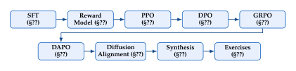
The chapter is organized as follows. Supervised Fine-Tuning covers supervised fine-tuning, the first stage of the alignment pipeline, including parameter-efficient methods such as LoRA. Reward Modelling develops the mathematics of reward modelling, showing how pairwise human preferences give rise to a reward function via the Bradley–Terry model. Proximal Policy Optimization for Alignment studies Proximal Policy Optimization as applied to language model alignment, deriving the KL-constrained objective and its optimal solution. Direct Preference Optimization presents Direct Preference Optimization, the key theoretical contribution of the chapter, building the derivation step by step from the reparameterization trick to the partition-function cancellation that eliminates the need for a reward model. Group Relative Policy Optimization introduces Group Relative Policy Optimization (GRPO), which eliminates the critic network, and DAPO: Alignment at Scale extends this to DAPO with four innovations for scaling. Alignment for Diffusion Models shows how these ideas transfer to diffusion model alignment. Connections and Synthesis synthesizes the landscape, and Exercises provides exercises.

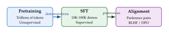
Roadmap for this chapter. We progress from supervised fine-tuning through reward modelling and reinforcement learning to direct preference methods and their extensions.

The three-stage pipeline that underlies most alignment work is illustrated in fig:alignment:pipeline. Each stage uses a different kind of data: pretraining consumes raw text at scale, SFT requires curated demonstrations, and alignment relies on pairwise preference judgments. The cost per datum increases at each stage, but the total data volume decreases by orders of magnitude.

The three-stage alignment pipeline. Pretraining provides broad capability on massive unlabeled data; supervised fine-tuning (SFT) teaches the model to follow instructions from curated demonstrations; alignment steers the model toward preferred outputs using human preference data. Data volume decreases while annotation cost per datum increases at each stage.

Supervised Fine-Tuning

The first stage of alignment is deceptively simple: take the pretrained language model and continue training it on a curated dataset of high-quality demonstrations. Each demonstration consists of a prompt (an instruction, question, or conversational context) paired with a desired response written by a human expert. This stage, known as supervised fine-tuning (SFT), transforms a base model that continues web text into a model that follows instructions.

Despite its simplicity, SFT has an outsized impact. Empirically, the jump in perceived quality from a base model to an SFT model is often larger than the subsequent jump from SFT to the aligned model. The reason is straightforward: SFT changes the format of the model's outputs, teaching it to respond to questions rather than complete documents, while alignment refines the quality within that format.

The SFT Objective

Definition 1 (Supervised Fine-Tuning Objective).

Given a dataset of demonstrations $𝒟_{SFT} = {(x^{(i)}, y^{(i)})}_{i = 1}^{N}$ where $x^{(i)}$ is a prompt and $y^{(i)} = (y_{1}^{(i)}, \dots, y_{T_{i}}^{(i)})$ is a response tokenized into $T_{i}$ tokens, the SFT loss is the negative log-likelihood of the response tokens conditioned on the prompt: (SFT LOSS) $\begin{matrix} ℒ_{SFT} (θ) = - \frac{1}{N} \sum_{i = 1}^{N} \sum_{t = 1}^{T_{i}} \log π_{θ} (y_{t}^{(i)} | x^{(i)}, y_{< t}^{(i)}), \end{matrix}$ where $π_{θ} (y_{t} | x, y_{< t})$ is the model's predicted probability of token $y_{t}$ given the prompt $x$ and all preceding response tokens $y_{< t} = (y_{1}, \dots, y_{t - 1})$ .

Remark 1 (SFT Is Next-Token Prediction).

The SFT objective is identical in form to the pretraining objective; both are next-token prediction via cross-entropy. The only difference is the data: pretraining uses raw web text, while SFT uses curated prompt–response pairs. In practice, the loss is typically computed only over the response tokens $y_{t}$ , not the prompt tokens $x$ , since we want the model to learn to generate responses, not to predict prompts. This is sometimes called prompt masking or completion-only training.

The SFT dataset is typically small by pretraining standards; InstructGPT used approximately 13,000 demonstrations [4], while Alpaca [15] used 52,000 instruction–response pairs generated by GPT-4. The key is not quantity but quality and diversity: the demonstrations must cover the range of tasks and response styles that we want the model to exhibit.

Training is straightforward: initialize from the pretrained checkpoint, set a small learning rate (typically $10^{- 5}$ to $10^{- 6}$ ), and train for 1–3 epochs. Overfitting is the primary concern: with only tens of thousands of examples, the model can memorize the training set within a single epoch.

Parameter-Efficient Fine-Tuning: LoRA

Full fine-tuning updates every parameter of the model, which poses two problems. First, it requires storing a full copy of the model gradients and optimizer states, which for a 70B-parameter model demands hundreds of gigabytes of GPU memory. Second, deploying multiple fine-tuned variants (one per task or customer) requires storing a separate copy of the full model for each variant.

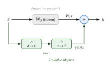
Low-Rank Adaptation (LoRA), introduced by Hu et al. [16], addresses both problems by freezing the pretrained weights and injecting small trainable low-rank matrices into each layer.

Definition 2 (Low-Rank Adaptation (LoRA)).

For a pretrained weight matrix $W_{0} \in ℝ^{d \times k}$ , LoRA reparameterizes the effective weight as (LORA Reparam) $\begin{matrix} W = W_{0} + Δ W = W_{0} + B A, \end{matrix}$ where $B \in ℝ^{d \times r}$ and $A \in ℝ^{r \times k}$ with $r ≪ \min (d, k)$ . The forward pass computes (LORA Forward) $\begin{matrix} h = W_{0} x + \frac{α}{r} B A x, \end{matrix}$ where $α > 0$ is a scaling hyperparameter. The matrices are initialized as $A \sim 𝒩 (0, σ^{2})$ and $B = 0$ , so that $Δ W = 0$ at initialization and the model begins from the pretrained weights. Only $A$ and $B$ are trained; $W_{0}$ is frozen.

The key insight is that the weight update $Δ W = B A$ has rank at most $r$ , so LoRA restricts the fine-tuning update to a low-rank subspace. This dramatically reduces the number of trainable parameters.

Proposition 1 (LoRA Parameter Reduction).

For a single weight matrix $W_{0} \in ℝ^{d \times k}$ , LoRA reduces the number of trainable parameters from $d k$ to $r (d + k)$ . The compression ratio is (LORA Compression) $\begin{matrix} \frac{d k}{r (d + k)} = \frac{d}{2 r} (for d = k) . \end{matrix}$ For typical values $d = k = 4096$ and $r = 8$ : full fine-tuning requires $4096 \times 4096 = 16,777,216$ parameters, while LoRA requires $8 \times (4096 + 4096) = 65,536$ parameters, a $256 \times$ reduction.

Proof.

The matrix $B \in ℝ^{d \times r}$ has $d r$ parameters and $A \in ℝ^{r \times k}$ has $r k$ parameters, giving $r (d + k)$ total. The ratio $d k / r (d + k)$ follows immediately. Substituting $d = k = 4096$ and $r = 8$ yields $16,777,216 / 65,536 = 256$ .

∎

LoRA architecture. The pretrained weight matrix

W_{0}

(gray) is frozen. A low-rank bypass path through the trainable down-projection

A

(dimension

d \to r

) and up-projection

B

(dimension

r \to d

) captures the task-specific update. At initialization,

B = 0

ensures that the model starts from the pretrained weights. The rank bottleneck

r ≪ d

compresses the adaptation into a tiny subspace.

Definition 3 (QLoRA).

QLoRA [6] combines LoRA with aggressive quantization of the frozen weights. The pretrained matrix $W_{0}$ is stored in 4-bit NormalFloat (NF4) format, a data type whose quantization levels are optimally spaced for normally distributed weights. QLoRA introduces two additional techniques: double quantization, which quantizes the quantization constants themselves to further reduce memory, and paged optimizers, which offload optimizer states to CPU memory when GPU memory is exhausted. The LoRA adapters $A$ and $B$ remain in 16-bit precision, so the gradient computation is unchanged. The result is that a 65B-parameter model can be fine-tuned on a single 48,GB GPU.

Example 1 (Fine-Tuning LLaMA-7B with LoRA).

Consider fine-tuning a LLaMA-7B model.

Full fine-tuning: 7 billion parameters $\times$ 2 bytes (FP16) $= 14$ ,GB of trainable parameters, plus optimizer states (Adam requires $2 \times$ the parameter memory), totaling $\sim$ 42,GB.
LoRA (rank 8): Apply LoRA to the query and value projection matrices in all 32 Transformer layers. Each layer has 2 matrices of size $4096 \times 4096$ , yielding $32 \times 2 \times 8 \times (4096 + 4096) \times 2$ bytes $\approx 8$ ,MB of trainable parameters.
Compression ratio: $14 GB / 8 MB \approx 1750 \times$ .

The LoRA-adapted model achieves comparable performance to full fine-tuning on instruction-following benchmarks while using approximately $0.06 %$ of the trainable parameter budget.

Insight.

LoRA exploits the hypothesis that weight updates during fine-tuning have low intrinsic dimensionality [7]: the effective number of parameters needed to capture task-specific knowledge is far smaller than the full parameter count. Aghajanyan et al. showed that pretrained models can be fine-tuned in a randomly projected subspace of dimension as low as a few hundred, with minimal loss in performance. LoRA provides a structured, hardware-efficient way to exploit this low-rank structure, replacing random projections with learned low-rank factors.

Remark 2 (Inference-Time Merging).

At inference time, the LoRA adapters can be merged into the base weights: $W = W_{0} + (α / r) B A$ . After merging, the forward pass is identical to that of a standard model with no additional latency or memory overhead. Moreover, multiple LoRA adapters (one per task) can be stored separately and swapped dynamically, enabling efficient multi-task serving from a single base model. This is sometimes called LoRA task routing and is the basis of systems like S-LoRA [8] that serve hundreds of LoRA adapters from a single GPU.

Reward Modelling

The SFT model follows instructions, but not all instructions are followed equally well. Given a prompt, the model might produce several plausible responses that differ in helpfulness, accuracy, tone, and safety. How do we teach the model which responses are better?

The answer is to learn a reward model from human preference data. Instead of asking humans to write perfect demonstrations (which is expensive and difficult to scale), we ask them a simpler question: given two responses, which one is better? This pairwise comparison format is cognitively easier for annotators, produces more consistent labels, and can be used to construct a scalar reward function that captures the aggregate structure of human preferences.

Preference Data

Definition 4 (Preference Dataset).

A preference dataset is a collection (Preference DATA) $\begin{matrix} 𝒟 = {(x^{(i)}, y_{w}^{(i)}, y_{l}^{(i)})}_{i = 1}^{N}, \end{matrix}$ where for each prompt $x^{(i)}$ , the response $y_{w}^{(i)}$ is preferred (“winning”) and $y_{l}^{(i)}$ is dispreferred (“losing”), as judged by a human annotator. We write $y_{w} ≻ y_{l} | x$ to denote the preference relation.

In practice, collecting preference data proceeds as follows: (1) sample a batch of prompts from a distribution of interest; (2) for each prompt, generate $K$ candidate responses from the current policy; (3) present pairs (or $K$ -tuples) of responses to human annotators and ask them to rank the responses; (4) convert the rankings into pairwise preferences.

The Bradley–Terry Model

To convert pairwise preferences into a trainable objective, we need a preference model: a probabilistic model of the annotator's choice. The most widely used model is the Bradley–Terry model, which dates to 1952 [17] and is also the foundation of the Elo rating system in chess.

Definition 5 (Bradley–Terry Preference Model).

Given a latent reward function $r_{ϕ} : 𝒳 \times 𝒴 \to ℝ$ parameterized by $ϕ$ , the Bradley–Terry model defines the probability that response $y_{w}$ is preferred over $y_{l}$ given prompt $x$ as (BT Model) $\begin{matrix} p (y_{w} ≻ y_{l} | x) = σ (r_{ϕ} (x, y_{w}) - r_{ϕ} (x, y_{l})), \end{matrix}$ where $σ (z) = 1 / (1 + e^{- z})$ is the logistic sigmoid function.

The Bradley–Terry model has a clean interpretation: the probability that $y_{w}$ is preferred depends only on the difference in rewards. If $r_{ϕ} (x, y_{w}) ≫ r_{ϕ} (x, y_{l})$ , then $σ (\cdot) \approx 1$ and preference for $y_{w}$ is near-certain. If the rewards are equal, the preference probability is exactly $1 / 2$ (a coin flip), as one would expect.

Reward Model Training

The reward model is trained by maximum likelihood under the Bradley–Terry model.

Definition 6 (Reward Model Loss).

The reward model training loss is the negative log-likelihood of the observed preferences under the Bradley–Terry model: (RM LOSS) $\begin{matrix} ℒ_{RM} (ϕ) = - 𝔼_{(x, y_{w}, y_{l}) \sim 𝒟} [\log σ (r_{ϕ} (x, y_{w}) - r_{ϕ} (x, y_{l}))] . \end{matrix}$ This is a binary cross-entropy loss where the “label” is always $1$ (since $y_{w}$ is always the preferred response by construction) and the “logit” is the reward difference $r_{ϕ} (x, y_{w}) - r_{ϕ} (x, y_{l})$ .

Remark 3 ( $K$ -way Rankings).

In practice, annotators often rank $K$ responses rather than comparing just two. Given $K$ responses ranked $y^{(1)} ≻ y^{(2)} ≻ \dots ≻ y^{(K)}$ , we form $(\binom{K}{2})$ pairwise comparisons. This is more data-efficient: $K$ responses yield $K (K - 1) / 2$ training pairs. InstructGPT uses $K = 4$ to $K = 9$ rankings per prompt, generating between 6 and 36 pairwise comparisons from each annotation [4]. To avoid correlated training examples, InstructGPT ensures that all pairs from a single ranking appear in the same training batch.

Proposition 2 (Reward Identifiability).

Under the Bradley–Terry model, the reward function $r (x, y)$ is identifiable only up to an input-dependent constant. That is, $r (x, y)$ and $r (x, y) + f (x)$ induce the same preference distribution for any function $f : 𝒳 \to ℝ$ .

Proof.

Substitute $r^{'} (x, y) = r (x, y) + f (x)$ into the Bradley–Terry model: (Reward Identifiability) $\begin{matrix} p^{'} (y_{w} ≻ y_{l} | x) & = σ (r^{'} (x, y_{w}) - r^{'} (x, y_{l})) \\ = σ (r (x, y_{w}) + f (x) - r (x, y_{l}) - f (x)) \\ = σ (r (x, y_{w}) - r (x, y_{l})) \\ = p (y_{w} ≻ y_{l} | x) . \end{matrix}$ The $f (x)$ terms cancel because the Bradley–Terry probability depends only on the reward difference, which is invariant to any additive function of the input alone. Therefore, without additional constraints (such as normalizing the reward to have zero mean per prompt), the reward is determined only up to this additive ambiguity.

∎

The reward model data collection and training pipeline. Prompts are sampled,

K

responses are generated from the current policy, a human annotator ranks them, the rankings are decomposed into pairwise preferences, and the reward model is trained on the resulting preference dataset.

Caution.

Goodhart's Law and Reward Hacking. “When a measure becomes a target, it ceases to be a good measure.” When the learned reward model $r_{ϕ}$ is optimized too aggressively, the policy may discover adversarial inputs to the reward model, outputs that score high on $r_{ϕ}$ but are low quality according to true human preferences. This phenomenon, known as reward hacking or reward overoptimization, is the alignment analogue of Goodhart's law. Empirically, Gao et al. [9] showed that reward model score initially tracks true preference quality as optimization proceeds, but eventually diverges: the policy finds reward-model-specific artifacts that inflate the score without improving actual quality. The KL penalty in the RLHF objective is the primary defense, limiting how far the policy can deviate from the reference and thereby bounding the extent of reward exploitation.

Example 2 (InstructGPT Reward Model).

InstructGPT [4] trains a 6B-parameter reward model, not the full 175B model. The RM is initialized from the SFT model checkpoint: the language model head (the unembedding matrix that projects hidden states to vocabulary logits) is removed and replaced with a linear projection to a scalar: (RM Architecture) $\begin{matrix} r_{ϕ} (x, y) = 𝒘^{⊤} 𝒉_{L} + b, \end{matrix}$ where $𝒉_{L} \in ℝ^{d}$ is the hidden state at the last token position of the concatenated input $(x, y)$ , and $𝒘 \in ℝ^{d}$ , $b \in ℝ$ are learned parameters. Using a smaller model (6B rather than 175B) for the reward model improves training stability and reduces the risk of overfitting to the relatively small preference dataset ( $\sim$ 33K comparisons).

Remark 4 (Reward Model Architecture).

The standard recipe for building a reward model is:

Initialize from the SFT model checkpoint (which has already learned useful representations of language quality).
Replace the language model head with a scalar projection $ℝ^{d} \to ℝ$ .
Train on preference data using the Bradley–Terry loss .
The reward for a prompt–response pair is the scalar output at the last token position.

This architecture has the advantage that the reward model “understands” language at a level comparable to the policy, since it shares the same pretrained backbone. However, it also means that the reward model has the same failure modes as the language model (hallucination, sensitivity to phrasing), which contributes to the reward hacking problem.

Proximal Policy Optimization for Alignment

With a reward model in hand, we can now formulate alignment as a reinforcement learning problem. The language model is the policy $π_{θ}$ , the prompt is the state, the generated response is the action, and the reward model provides the reward signal. The goal is to update the policy to maximize the expected reward while staying close to the pretrained reference policy.

The KL-Constrained Objective

Definition 7 (KL-Constrained Reward Maximization).

The alignment objective is (RLHF Objective) $\begin{matrix} \max_{π_{θ}} 𝔼_{x \sim 𝒟, y \sim π_{θ} (\cdot | x)} [r_{ϕ} (x, y)] - β D_{KL} [π_{θ} (\cdot | x) ‖ π_{ref} (\cdot | x)], \end{matrix}$ where $π_{ref}$ is the SFT policy (frozen after Stage 1), $r_{ϕ}$ is the reward model (frozen after Stage 2), and $β > 0$ controls the strength of the KL constraint. The KL divergence is (KL DIV) $\begin{matrix} D_{KL} [π_{θ} (\cdot | x) ‖ π_{ref} (\cdot | x)] = 𝔼_{y \sim π_{θ} (\cdot | x)} [\log \frac{π_{θ} (y | x)}{π_{ref} (y | x)}] . \end{matrix}$

The KL term serves two purposes. First, it prevents reward hacking: by limiting how far the policy can deviate from the reference, it bounds the extent to which the policy can exploit artifacts of the learned reward model (see warn:goodhart). Second, it preserves the general capabilities acquired during pretraining: without the KL constraint, aggressive reward maximization can cause the model to forget how to perform tasks that are not directly rewarded, a phenomenon known as catastrophic forgetting.

The Optimal Policy

The KL-constrained objective has a remarkably clean closed-form solution, which will play a central role in the DPO derivation (Direct Preference Optimization).

Theorem 1 (Optimal Policy under KL Constraint).

The optimal policy for the KL-constrained objective is (Optimal Policy) $\begin{matrix} π^{*} (y | x) = \frac{1}{Z (x)} π_{ref} (y | x) \exp (\frac{r (x, y)}{β}), \end{matrix}$ where the partition function is (Partition Function) $\begin{matrix} Z (x) = \sum_{y} π_{ref} (y | x) \exp (\frac{r (x, y)}{β}) . \end{matrix}$

Proof.

We seek to maximize the functional (J Functional) $\begin{matrix} J [π] = \sum_{y} π (y | x) r (x, y) - β \sum_{y} π (y | x) \log \frac{π (y | x)}{π_{ref} (y | x)}, \end{matrix}$ subject to the constraint $\sum_{y} π (y | x) = 1$ . Introducing a Lagrange multiplier $λ$ for the normalization constraint, we form the Lagrangian (Lagrangian) $\begin{matrix} ℒ [π, λ] = \sum_{y} π (y | x) [r (x, y) - β \log \frac{π (y | x)}{π_{ref} (y | x)}] + λ (1 - \sum_{y} π (y | x)) . \end{matrix}$ Taking the functional derivative with respect to $π (y | x)$ for a fixed $y$ and setting it to zero: (Lagrangian Deriv) $\begin{matrix} \frac{\partial ℒ}{\partial π (y | x)} & = r (x, y) - β \log \frac{π (y | x)}{π_{ref} (y | x)} - β - λ = 0. \end{matrix}$ Solving for $π (y | x)$ : (LOG Ratio) $\begin{matrix} \log \frac{π (y | x)}{π_{ref} (y | x)} = \frac{r (x, y) - β - λ}{β}, \end{matrix}$ and exponentiating: (Unnormalized) $\begin{matrix} π (y | x) = π_{ref} (y | x) \exp (\frac{r (x, y)}{β}) \exp (\frac{- β - λ}{β}) . \end{matrix}$ The factor $\exp ((- β - λ) / β)$ is independent of $y$ and serves as the normalization constant. Defining $Z (x) = \exp ((β + λ) / β)$ and enforcing $\sum_{y} π (y | x) = 1$ recovers (Partition Function).

To verify this is a maximum, note that $J [π]$ is strictly concave in $π$ (as the sum of a linear term and a negative KL divergence, which is strictly concave), so the unique stationary point is the global maximum.

∎

The optimal policy has an intuitive interpretation: it is the reference policy reweighted by the exponentiated reward. Responses with high reward are upweighted, responses with low reward are downweighted, and the temperature $β$ controls the sharpness of this reweighting. As $β \to 0$ , the policy concentrates on the reward-maximizing response; as $β \to \infty$ , the policy converges to $π_{ref}$ .

Per-Token Reward and the PPO Objective

In practice, the reward model assigns a single scalar $r_{ϕ} (x, y)$ to the entire response. To apply token-level policy gradient methods, we distribute this reward across tokens. The standard approach combines the KL penalty at each step with the final reward at the last token.

The per-token reward is defined as (PER Token Reward) $\begin{matrix} R_{t} = {\begin{matrix} - β \log \frac{π_{θ} (y_{t} | x, y_{< t})}{π_{ref} (y_{t} | x, y_{< t})} & if t < T, \\ r_{ϕ} (x, y) - β \log \frac{π_{θ} (y_{T} | x, y_{< T})}{π_{ref} (y_{T} | x, y_{< T})} & if t = T . \end{matrix} \end{matrix}$ At each intermediate step, the reward is the negative KL penalty: the cost of deviating from the reference policy. At the final step, the reward model score is added. The total reward $\sum_{t = 1}^{T} R_{t} = r_{ϕ} (x, y) - β \sum_{t = 1}^{T} \log (π_{θ} (y_{t} | x, y_{< t}) / π_{ref} (y_{t} | x, y_{< t}))$ equals the sequence-level objective , so optimizing the per-token formulation is equivalent to optimizing the original objective.

The policy is then updated using the PPO clipped objective: (PPO CLIP) $\begin{matrix} ℒ_{PPO} (θ) = 𝔼_{t} [\min (r_{t} (θ) {\hat{A}}_{t}, clip (r_{t} (θ), 1 - ϵ, 1 + ϵ) {\hat{A}}_{t})], \end{matrix}$ where (PPO Ratio) $\begin{matrix} r_{t} (θ) = \frac{π_{θ} (y_{t} | y_{< t}, x)}{π_{old} (y_{t} | y_{< t}, x)} \end{matrix}$ is the importance sampling ratio between the current and old policies, ${\hat{A}}_{t}$ is the generalized advantage estimate (GAE), and $ϵ$ (typically $0.2$ ) is the clipping range. The $\min$ and $clip$ operations ensure that the policy does not change too much in a single update, stabilizing training.

Definition 8 (PPO-ptx: Pretraining Loss Mixing).

To prevent catastrophic forgetting of general capabilities, InstructGPT augments the PPO objective with a pretraining loss: (PPO PTX) $\begin{matrix} J (θ) = J_{PPO} (θ) + γ 𝔼_{x \sim 𝒟_{pretrain}} [\log π_{θ} (x)], \end{matrix}$ where $γ > 0$ balances alignment with capability preservation and $𝒟_{pretrain}$ is a sample of pretraining data. InstructGPT uses $γ = 27.8$ , indicating that preserving general capabilities is weighted heavily relative to the PPO signal.

The InstructGPT Pipeline

Algorithm 1 (InstructGPT RLHF Pipeline).

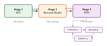
The full InstructGPT training pipeline consists of three stages:

Stage 1 - Supervised Fine-Tuning (SFT):

Collect a dataset of $\sim$ 13K prompt–demonstration pairs from human labelers.
Fine-tune the pretrained GPT-3 model on this dataset using the SFT loss for 16 epochs.
Select the checkpoint with highest validation reward model score (not lowest validation loss).

Stage 2 - Reward Model (RM) Training:

For each of $\sim$ 33K prompts, generate $K \in {4, \dots, 9}$ responses from the SFT model.
Have human labelers rank the $K$ responses.
Decompose rankings into $(\binom{K}{2})$ pairwise preferences.
Initialize a 6B model from the SFT checkpoint, replace the LM head with a scalar projection, and train using the Bradley–Terry loss .

Stage 3 - PPO:

Initialize the policy $π_{θ}$ from the SFT model.
Initialize the value function (critic) from the RM weights.
For each PPO iteration: enumerate[label=()]
Sample a batch of prompts $x \sim 𝒟$ .
Generate responses $y \sim π_{θ} (\cdot | x)$ .
Compute rewards $R_{t}$ using .
Compute advantages ${\hat{A}}_{t}$ using GAE.
Update the policy using the PPO-ptx objective .
Update the value function to minimize the value loss. enumerate

The InstructGPT three-stage pipeline. Stage 1 (green) produces the SFT model from human demonstrations. Stage 2 (orange) trains a reward model on preference rankings. Stage 3 (purple) optimizes the policy with PPO, using the RL loop shown below: generate responses, compute rewards, and update the policy.

Example 3 (Reward Hacking Without KL Penalty).

Consider what happens when $β = 0$ in (RLHF Objective), pure reward maximization with no KL constraint. The policy is free to deviate arbitrarily from $π_{ref}$ . In practice, this leads to degenerate behaviour. For instance, a helpfulness reward model might assign high scores to effusively positive responses (“I'm so happy to help you with this wonderful question!”) regardless of content. Without the KL penalty, the policy quickly converges to producing such responses for every prompt, achieving high reward-model scores while being completely useless. With $β > 0$ , the KL penalty charges a cost for this deviation: the model cannot stray far from the reference policy's distribution, which includes diverse and substantive responses. The result is a model that is somewhat more helpful (high reward) while remaining broadly capable (low KL from reference).

Remark 5 (Critic Initialization).

The value function (critic) in PPO estimates the expected future reward $V (x, y_{< t}) = 𝔼 [\sum_{t^{'} = t}^{T} R_{t^{'}} | x, y_{< t}]$ . In InstructGPT, the critic is initialized from the reward model weights. This gives the critic a significant head start: the RM has already learned to evaluate response quality, so the initial value estimates are meaningful rather than random. This initialization is crucial for stable training, as random critic values lead to high variance in the advantage estimates and erratic policy updates.

Remark 6 (InstructGPT Results).

The InstructGPT paper [4] reported a striking result: a 1.3B-parameter InstructGPT model was preferred over the 175B-parameter GPT-3 base model by human evaluators 85% of the time. This demonstrated that alignment can compensate for orders-of-magnitude differences in model size: a well-aligned small model can be more useful than a poorly aligned large one. The result catalyzed the field, demonstrating that the bottleneck for useful AI systems was not just scale but alignment.

Direct Preference Optimization

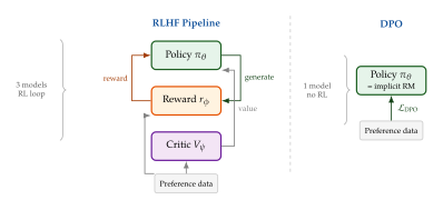
The RLHF pipeline described in Proximal Policy Optimization for Alignment works, but it is complex. It requires training three separate models (the SFT policy, the reward model, and the PPO critic), managing an online RL loop with all its instabilities (reward hacking, value function divergence, hyperparameter sensitivity), and running four neural networks simultaneously during training (the policy, the reference policy, the reward model, and the critic). Each of these components introduces potential points of failure, and the overall system is notoriously difficult to tune.

Direct Preference Optimization (DPO), introduced by Rafailov et al. (2023) [5], makes a beautiful observation: the reward model and the RL loop are unnecessary. By exploiting the closed-form solution for the optimal policy (Theorem 1), DPO reparameterizes the reward in terms of the policy and eliminates the reward model entirely. The result is a simple, stable, supervised-learning objective that directly optimizes the policy on preference data.

Recap: From Bradley–Terry to the KL-Constrained Objective

Let us briefly review the key results from Reward Modelling and Proximal Policy Optimization for Alignment that DPO builds upon.

The Bradley–Terry model (Definition 5) gives the probability of preference in terms of a latent reward: (DPO BT Recap) $\begin{matrix} p (y_{w} ≻ y_{l} | x) = σ (r (x, y_{w}) - r (x, y_{l})) . \end{matrix}$

The KL-constrained alignment objective (Definition 7) is (DPO KL Recap) $\begin{matrix} \max_{π_{θ}} 𝔼_{x, y \sim π_{θ}} [r (x, y)] - β D_{KL} [π_{θ} ‖ π_{ref}], \end{matrix}$ and its optimal solution (Theorem 1) is (DPO Optimal Recap) $\begin{matrix} π^{*} (y | x) = \frac{1}{Z (x)} π_{ref} (y | x) \exp (r (x, y) / β) . \end{matrix}$

The standard RLHF pipeline uses (DPO BT Recap) to train a reward model, then uses the reward model in (DPO KL Recap) to train the policy with PPO. DPO takes a different path.

The Reparameterization Trick

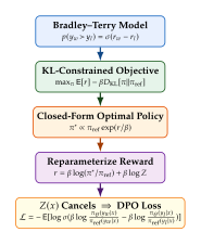
The key insight begins with a simple algebraic manipulation. Starting from the optimal policy , take the logarithm of both sides: (DPO LOG Optimal) $\begin{matrix} \log π^{*} (y | x) = \log π_{ref} (y | x) + \frac{r (x, y)}{β} - \log Z (x) . \end{matrix}$ Now solve for the reward: (DPO Reward Reparam) $\begin{matrix} r (x, y) = β \log \frac{π^{*} (y | x)}{π_{ref} (y | x)} + β \log Z (x) . \end{matrix}$

This is the reparameterization: the reward is expressed purely in terms of the optimal policy $π^{*}$ , the reference policy $π_{ref}$ , and the partition function $Z (x)$ . The reward model has been eliminated, replaced by the log-ratio of the optimal and reference policies, plus a prompt-dependent constant.

Remark 7.

Equation should be compared with the reward identifiability result (Proposition 2): the reward is only identifiable up to an input-dependent constant, and here that constant is $β \log Z (x)$ . This ambiguity is harmless for pairwise preferences, as we will see in the next subsection.

Partition Function Cancellation

Now substitute the reparameterized reward into the Bradley–Terry model : (DPO Cancel) $\begin{matrix} p (y_{w} ≻ y_{l} | x) & = σ (r (x, y_{w}) - r (x, y_{l})) \\ = σ (β \log \frac{π^{*} (y_{w} | x)}{π_{ref} (y_{w} | x)} + β \log Z (x) - β \log \frac{π^{*} (y_{l} | x)}{π_{ref} (y_{l} | x)} - β \log Z (x)) \\ = σ (β \log \frac{π^{*} (y_{w} | x)}{π_{ref} (y_{w} | x)} - β \log \frac{π^{*} (y_{l} | x)}{π_{ref} (y_{l} | x)}) . \end{matrix}$ The $β \log Z (x)$ terms cancel. This cancellation is the mathematical heart of DPO: the intractable partition function, which would require summing over all possible responses, simply disappears in the pairwise preference setting. No approximation is needed; the cancellation is exact.

The DPO Loss

With the partition function gone, we can replace the true optimal policy $π^{*}$ with our parameterized policy $π_{θ}$ (since we are optimizing $π_{θ}$ to approach $π^{*}$ ) and write down a loss function directly.

Definition 9 (DPO Loss).

The Direct Preference Optimization loss is (DPO LOSS) $\begin{matrix} ℒ_{DPO} (π_{θ}; π_{ref}) = - 𝔼_{(x, y_{w}, y_{l}) \sim 𝒟} [\log σ (β \log \frac{π_{θ} (y_{w} | x)}{π_{ref} (y_{w} | x)} - β \log \frac{π_{θ} (y_{l} | x)}{π_{ref} (y_{l} | x)})] . \end{matrix}$

Let us unpack this expression. Define the implicit reward of a response under the current policy: (Implicit Reward) $\begin{matrix} {\hat{r}}_{θ} (x, y) \overset{def}{=} β \log \frac{π_{θ} (y | x)}{π_{ref} (y | x)} . \end{matrix}$ Then the DPO loss simplifies to (DPO LOSS Simple) $\begin{matrix} ℒ_{DPO} = - 𝔼 [\log σ ({\hat{r}}_{θ} (x, y_{w}) - {\hat{r}}_{θ} (x, y_{l}))], \end{matrix}$ which is precisely the Bradley–Terry loss with the explicit reward $r_{ϕ}$ replaced by the implicit reward ${\hat{r}}_{θ}$ . The DPO loss is a binary cross-entropy loss that encourages the policy to assign higher implicit reward to the preferred response than to the dispreferred response.

Theorem 2 (DPO–RLHF Equivalence).

In the limit of infinite data and infinite model capacity, the global minimizer of the DPO loss is the same policy $π^{*}$ that would be obtained by the full RLHF pipeline: training a reward model with the Bradley–Terry loss and then optimizing the KL-constrained objective to convergence.

Proof sketch.

The DPO loss is derived by substituting the closed-form optimal policy into the Bradley–Terry likelihood. The derivation is exact; no approximations are made. Therefore, the population-level DPO loss is minimized when $π_{θ} = π^{*}$ , the same policy that simultaneously (a) satisfies the Bradley–Terry model under the true reward and (b) solves the KL-constrained optimization. In the finite-sample or finite-capacity regime, DPO and RLHF may converge to different solutions due to different optimization landscapes and regularization properties, but the population-level optima coincide.

∎

Gradient Analysis

Understanding the gradient of the DPO loss reveals an elegant self-weighting mechanism.

Proposition 3 (DPO Gradient).

The gradient of the DPO loss with respect to $θ$ is (DPO Gradient) $\begin{matrix} \nabla_{θ} ℒ_{DPO} = - β 𝔼_{(x, y_{w}, y_{l}) \sim 𝒟} [\underset{weighting factor}{\underset{⏟}{σ ({\hat{r}}_{θ} (x, y_{l}) - {\hat{r}}_{θ} (x, y_{w}))}} (\nabla_{θ} \log π_{θ} (y_{w} | x) - \nabla_{θ} \log π_{θ} (y_{l} | x))], \end{matrix}$ where ${\hat{r}}_{θ} (x, y) = β \log (π_{θ} (y | x) / π_{ref} (y | x))$ is the implicit reward.

Proof.

Starting from the DPO loss , let $u = {\hat{r}}_{θ} (x, y_{w}) - {\hat{r}}_{θ} (x, y_{l})$ . Then $ℒ_{DPO} = - 𝔼 [\log σ (u)]$ . Using $\frac{d}{d u} \log σ (u) = 1 - σ (u) = σ (- u)$ , we have (DPO GRAD Step1) $\begin{matrix} \nabla_{θ} ℒ_{DPO} = - 𝔼 [σ (- u) \nabla_{θ} u] = - 𝔼 [σ ({\hat{r}}_{θ} (x, y_{l}) - {\hat{r}}_{θ} (x, y_{w})) \nabla_{θ} u] . \end{matrix}$ Now compute $\nabla_{θ} u$ : (DPO GRAD Step2) $\begin{matrix} \nabla_{θ} u & = \nabla_{θ} [{\hat{r}}_{θ} (x, y_{w}) - {\hat{r}}_{θ} (x, y_{l})] \\ = β \nabla_{θ} [\log π_{θ} (y_{w} | x) - \log π_{θ} (y_{l} | x)] \\ = β [\nabla_{θ} \log π_{θ} (y_{w} | x) - \nabla_{θ} \log π_{θ} (y_{l} | x)], \end{matrix}$ since $π_{ref}$ does not depend on $θ$ . Substituting into yields .

∎

The gradient has a beautiful interpretation. The update increases the log-probability of the preferred response $y_{w}$ and decreases the log-probability of the dispreferred response $y_{l}$ . But the magnitude of the update is controlled by the sigmoid weighting factor $σ ({\hat{r}}_{y_{l}} - {\hat{r}}_{y_{w}})$ , which is large when the model currently assigns higher implicit reward to the wrong response ( ${\hat{r}}_{y_{l}} > {\hat{r}}_{y_{w}}$ ) and small when the model already gets it right ( ${\hat{r}}_{y_{w}} > {\hat{r}}_{y_{l}}$ ). This is automatic hard-example mining: the gradient focuses on the pairs that the model currently ranks incorrectly, and ignores the easy pairs that are already correct.

Proposition 4 (Implicit Reward Model).

After DPO training, the policy itself encodes a reward model: (Implicit RM) $\begin{matrix} r (x, y) = β \log \frac{π_{θ} (y | x)}{π_{ref} (y | x)} + β \log Z (x), \end{matrix}$ where $Z (x)$ is an input-dependent constant. Since preferences depend only on reward differences (Proposition 2), the $Z (x)$ term is irrelevant for ranking responses, and the log-ratio $\log (π_{θ} (y | x) / π_{ref} (y | x))$ serves as a fully functional reward model.

Insight.

DPO converts an RL problem into a classification problem. Instead of training three models (policy, reward model, critic) and running an online RL loop with all its instabilities, DPO trains a single model with a binary cross-entropy-style loss on static preference data. The reward model is not eliminated; it is absorbed into the policy. Every DPO-trained policy is a reward model (up to an irrelevant constant), accessible via the log-ratio in (Implicit RM). This duality between policies and reward models is the fundamental insight underlying DPO.

The DPO derivation as a logical flow. Starting from the Bradley–Terry preference model and the KL-constrained objective, we derive the closed-form optimal policy, reparameterize the reward in terms of the policy, and observe that the partition function

Z (x)

cancels in pairwise comparisons, yielding the DPO loss directly.

RLHF vs. DPO: a structural comparison. Left: the RLHF pipeline requires three models (policy, reward model, critic) connected in an online RL loop. Right: DPO requires only the policy, which is trained with a supervised loss on static preference data. The reward model is absorbed into the policy via the implicit reward (Proposition 4).

The DPO Algorithm

Algorithm 2 (DPO Training).

Input: Reference policy $π_{ref}$ (the SFT model), preference dataset $𝒟 = {(x^{(i)}, y_{w}^{(i)}, y_{l}^{(i)})}$ , temperature $β > 0$ , learning rate $η$ .

Procedure:

Initialize $π_{θ} \leftarrow π_{ref}$ .
Freeze $π_{ref}$ (no gradient updates).
For each mini-batch $(x, y_{w}, y_{l}) \sim 𝒟$ : enumerate[label=()]
Compute log-probabilities under $π_{θ}$ : $\log π_{θ} (y_{w} | x)$ and $\log π_{θ} (y_{l} | x)$ .
Compute log-probabilities under $π_{ref}$ (forward pass, no gradient): $\log π_{ref} (y_{w} | x)$ and $\log π_{ref} (y_{l} | x)$ .
Compute implicit rewards: ${\hat{r}}_{w} = β (\log π_{θ} (y_{w} | x) - \log π_{ref} (y_{w} | x))$ , ${\hat{r}}_{l} = β (\log π_{θ} (y_{l} | x) - \log π_{ref} (y_{l} | x))$ .
Compute loss: $ℒ = - \log σ ({\hat{r}}_{w} - {\hat{r}}_{l})$ .
Update: $θ \leftarrow θ - η \nabla_{θ} ℒ$ . enumerate
Output: Aligned policy $π_{θ}$ .

The simplicity of Algorithm 2 is remarkable compared to the InstructGPT pipeline (Algorithm 1). There is no reward model to train, no critic to initialize, no online generation loop, and no GAE computation. The entire alignment procedure reduces to computing log-probabilities under two models (the policy and the frozen reference) and backpropagating through a binary cross-entropy loss.

Example 4 (DPO vs. PPO on Summarization).

On the TL;DR summarization task [3], Rafailov et al. reported the following results:

DPO achieves a win rate of $\sim$ 61% against the SFT baseline (as judged by GPT-4).
PPO (best of sweep) achieves a win rate of $\sim$ 57% against the same baseline.
DPO uses approximately $3 \times$ less compute than PPO, since it avoids online generation and reward model inference during training.

The fact that DPO matches or exceeds PPO while being dramatically simpler was a key factor in its rapid adoption.

Remark 8 (Choice of $β$ ).

The temperature parameter $β$ controls how far the aligned policy can deviate from the reference. The effects are as follows:

Small $β$ (e.g., $β = 0.1$ ): aggressive optimization. The implicit reward is amplified, so the policy can move far from $π_{ref}$ to maximize preference alignment. Risk: overfitting to preference data, reduced diversity, potential reward hacking.
Large $β$ (e.g., $β = 0.5$ ): conservative optimization. The policy stays close to $π_{ref}$ , making small adjustments. Risk: underfitting, failing to fully capture human preferences.
Typical range: $β \in [0.1, 0.5]$ . Rafailov et al. use $β = 0.1$ for summarization and $β = 0.5$ for dialogue.

Remark 9 (DPO Limitations).

Despite its elegance, DPO has known limitations:

Distribution shift: DPO trains on offline preference data (generated by the SFT policy or a previous checkpoint), but the policy $π_{θ}$ evolves during training. As $π_{θ}$ diverges from the data-generating policy, the preference pairs become less informative, and the model may learn to distinguish responses that it would never generate. Online variants such as online DPO and iterative DPO address this by periodically regenerating preference data from the current policy.
Reference policy dependence: The DPO loss depends on $π_{ref}$ through the log-ratio. If $π_{ref}$ assigns near-zero probability to a response in the preference data, the log-ratio becomes very large, leading to numerical instability. In practice, this requires careful filtering of preference data to ensure both responses are plausible under $π_{ref}$ .
No exploration: Unlike PPO, which generates new responses during training and can discover novel high-reward strategies, DPO is limited to the behaviors represented in the static preference dataset. This can be a significant disadvantage for tasks where the optimal strategy is not well represented in the training data.

We summarize the comparison between RLHF (PPO) and DPO in Table 1.

Aspect	RLHF (PPO)	DPO
Models required	Policy + Reward Model + Critic (3)	Policy only (1)
Training data	Online (generated during training)	Offline (static preference dataset)
Reward model	Explicit, separately trained	Implicit in the policy
Optimization	Reinforcement learning (policy gradient)	Supervised learning (cross-entropy)
Partition function	Approximated (not needed explicitly)	Cancels exactly in pairwise comparisons
Hyperparameters	Many (PPO clip, GAE $λ$ , critic lr, )	Few ( $β$ , learning rate)
Compute cost	High (4 forward passes per step)	Low (2 forward passes per step)
Exploration	Yes (online generation)	No (offline data)
Reward hacking	Controlled by KL penalty	Implicitly controlled by $β$
Distribution shift	Mitigated by online sampling	Can be problematic

Comparison of RLHF (PPO) and DPO for language model alignment.

Group Relative Policy Optimization

The PPO algorithm described in Proximal Policy Optimization for Alignment requires maintaining four neural networks simultaneously during training: the policy $π_{θ}$ , the reference policy $π_{ref}$ , the reward model $r_{ϕ}$ , and a critic (value function) $V_{ψ}$ . The critic alone can be as large as the policy itself, doubling the GPU memory required. For models at the 70B–671B parameter scale, this cost is prohibitive: a 671B policy would require two copies of itself (policy + critic) plus a reward model, easily exceeding the memory of an entire compute cluster.

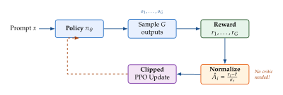
Group Relative Policy Optimization (GRPO), introduced by Shao et al. (2024) [18] in the context of DeepSeekMath, eliminates the critic entirely by computing advantages relative to a group of sampled outputs. The key insight is disarmingly simple: instead of learning a value function to estimate the advantage, just sample multiple outputs for the same prompt and normalize their rewards.

Key Idea.

Group-based advantage estimation. Given a prompt $x$ , sample a group of $G$ candidate outputs ${o_{1}, o_{2}, \dots, o_{G}}$ from the current policy $π_{θ}$ . Score each output with the reward model to obtain ${r_{1}, r_{2}, \dots, r_{G}}$ . The advantage of output $o_{i}$ is simply its z-scored reward within the group: ${\hat{A}}_{i} = \frac{r_{i} - \overline{r}}{σ_{r}}, \overline{r} = \frac{1}{G} \sum_{j = 1}^{G} r_{j}, σ_{r} = \sqrt{\frac{1}{G} \sum_{j = 1}^{G} {(r_{j} - \overline{r})}^{2}} .$ No learned value function is needed; the group is the baseline.

From PPO to GRPO

Recall the PPO objective from (PPO CLIP). In standard PPO, the advantage ${\hat{A}}_{t}$ at each token is estimated using Generalized Advantage Estimation (GAE), which requires the value function $V_{ψ}$ . GRPO replaces this with a constant advantage across all tokens in a given output: every token in output $o_{i}$ receives the same advantage ${\hat{A}}_{i}$ .

Definition 10 (GRPO Objective).

Given a prompt $x$ , group of outputs ${o_{1}, \dots, o_{G}}$ sampled from the old policy $π_{θ_{old}}$ , and group-normalized advantages ${{\hat{A}}_{1}, \dots, {\hat{A}}_{G}}$ , the GRPO objective is: (GRPO Objective) $\begin{matrix} J_{GRPO} (θ) = \frac{1}{G} \sum_{i = 1}^{G} \frac{1}{| o_{i} |} \sum_{t = 1}^{| o_{i} |} [\min (ρ_{i, t} {\hat{A}}_{i}, clip (ρ_{i, t}, 1 - ϵ, 1 + ϵ) {\hat{A}}_{i}) - β D_{KL}^{(i, t)}], \end{matrix}$ where the importance ratio is $ρ_{i, t} = π_{θ} (o_{i, t} | x, o_{i, < t}) / π_{θ_{old}} (o_{i, t} | x, o_{i, < t})$ , $ϵ$ is the clipping threshold (typically $0.2$ ), and the per-token KL divergence uses the unbiased estimator (GRPO KL) $\begin{matrix} D_{KL}^{(i, t)} = \frac{π_{ref} (o_{i, t} | x, o_{i, < t})}{π_{θ} (o_{i, t} | x, o_{i, < t})} - \log \frac{π_{ref} (o_{i, t} | x, o_{i, < t})}{π_{θ} (o_{i, t} | x, o_{i, < t})} - 1. \end{matrix}$

Remark 10 (Unbiased KL Estimator).

The estimator in (GRPO KL) is derived from the identity $D_{KL} [p ‖ q] = 𝔼_{p} [\log (p / q)]$ . Let $u = q (x) / p (x)$ where $x \sim p$ . Then $𝔼_{p} [u - \log u - 1] = D_{KL} [p ‖ q]$ , since $𝔼_{p} [u] = \sum_{x} p (x) \cdot q (x) / p (x) = 1$ and $𝔼_{p} [- \log u] = 𝔼_{p} [\log (p / q)] = D_{KL} [p ‖ q]$ . The estimator $u - \log u - 1 \geq 0$ for all $u > 0$ (with equality at $u = 1$ ), so each sample provides a non-negative, unbiased estimate of the KL divergence. This avoids the variance issues of the naive estimator $\log (p / q)$ when $p$ and $q$ are close.

Outcome Supervision vs. Process Supervision

GRPO is particularly effective for tasks with verifiable rewards (mathematics, coding, formal logic) where the correctness of the final answer can be checked automatically. In this setting, two supervision strategies are natural:

Outcome supervision: The reward depends only on the final answer: $r_{i} = 𝟏 [answer (o_{i}) is correct]$ . This is cheap to implement but provides a sparse signal.
Process supervision: The reward incorporates intermediate reasoning steps, e.g., checking each line of a mathematical derivation. This provides a denser signal but requires a process reward model (PRM) or step-level verification.

DeepSeekMath [18] demonstrates that GRPO with outcome supervision alone achieves 51.7% accuracy on the MATH benchmark, competitive with GPT-4 on mathematical reasoning, using a 7B parameter model. The group-based normalization ensures that even with binary (correct/incorrect) rewards, the advantage signal is informative: within any group, correct solutions receive positive advantage and incorrect ones receive negative advantage.

Proposition 5 (GRPO Advantage with Binary Rewards).

If the reward is binary, $r_{i} \in {0, 1}$ , and $k$ out of $G$ outputs in the group are correct ( $0 < k < G$ ), then: ${\hat{A}}_{i} = {\begin{matrix} \frac{1 - k / G}{\sqrt{k (G - k) / G^{2}}} = \sqrt{\frac{G - k}{k}} & if o_{i} is correct, \\ \frac{0 - k / G}{\sqrt{k (G - k) / G^{2}}} = - \sqrt{\frac{k}{G - k}} & if o_{i} is incorrect . \end{matrix}$ The advantage magnitude is larger for the minority class: if few outputs are correct ( $k ≪ G$ ), correct outputs receive large positive advantage; if few are incorrect ( $k \approx G$ ), incorrect outputs receive large negative advantage.

Proof.

The group mean is $\overline{r} = k / G$ and the variance is $σ_{r}^{2} = \frac{1}{G} \sum_{i} {(r_{i} - k / G)}^{2} = \frac{k}{G} {(1 - k / G)}^{2} + \frac{G - k}{G} {(k / G)}^{2} = \frac{k (G - k)}{G^{2}}$ . For a correct output, ${\hat{A}}_{i} = (1 - k / G) / σ_{r} = (G - k) / (G σ_{r}) = \sqrt{(G - k) / k}$ . For an incorrect output, ${\hat{A}}_{i} = (0 - k / G) / σ_{r} = - k / (G σ_{r}) = - \sqrt{k / (G - k)}$ .

∎

Example 5 (GRPO in Action: Mathematical Reasoning).

Consider the prompt: “Solve $\int_{0}^{1} x^{2} e^{x} d x$ .” We sample $G = 8$ candidate outputs from the policy. Suppose 3 outputs arrive at the correct answer $e - 2$ and 5 produce incorrect results. The rewards are $r \in {1, 1, 1, 0, 0, 0, 0, 0}$ with $\overline{r} = 3 / 8$ , $σ_{r} = \sqrt{15 / 64} \approx 0.484$ . The advantages are: $\begin{matrix} {\hat{A}}_{correct} & = \frac{1 - 3 / 8}{0.484} \approx + 1.29 & (reinforce these outputs), \\ {\hat{A}}_{incorrect} & = \frac{0 - 3 / 8}{0.484} \approx - 0.77 & (suppress these outputs) . \end{matrix}$ The correct (minority) outputs receive a larger magnitude advantage, ensuring the policy updates focus on amplifying rare successful strategies. No value function was needed; the group provided its own baseline.

The GRPO pipeline. A group of

G

outputs is sampled, scored by the reward model, z-score normalized within the group to produce advantages, and used in a clipped PPO-style update. The critic is eliminated entirely.

PPO vs. GRPO: A Comparison

Aspect	PPO	GRPO
Advantage estimation	Learned critic $V_{ψ}$ (GAE)	Group z-score normalization
Models in memory	Policy + Critic + Reward + Reference (4)	Policy + Reward + Reference (3)
Memory saving	Baseline	$\sim$ 50% (no critic)
Token-level advantage	Yes (different ${\hat{A}}_{t}$ per token)	No (same ${\hat{A}}_{i}$ for all tokens)
KL regularization	Reward penalty or PPO constraint	Explicit KL term per token
Best suited for	General RLHF, creative tasks	Verifiable tasks (math, code)

Comparison of PPO and GRPO for language model alignment.

Algorithm 3 (GRPO Training).

Input: Prompt dataset $𝒟$ , initial policy $π_{θ}$ , reference policy $π_{ref}$ , reward model $r_{ϕ}$ , group size $G$ , clip threshold $ϵ$ , KL coefficient $β$
for iteration $= 1, 2, \dots$
Sample a batch of prompts ${x^{(1)}, \dots, x^{(B)}} \sim 𝒟$
for each prompt $x^{(j)}$
Sample $G$ outputs: $o_{1}, \dots, o_{G} \sim π_{θ_{old}} (\cdot | x^{(j)})$
Compute rewards: $r_{i} = r_{ϕ} (x^{(j)}, o_{i})$ for $i = 1, \dots, G$
Normalize: ${\hat{A}}_{i} = (r_{i} - \overline{r}) / σ_{r}$
Compute $J_{GRPO} (θ)$ via (GRPO Objective)
Update $θ \leftarrow θ + α \nabla_{θ} J_{GRPO} (θ)$
Update old policy: $θ_{old} \leftarrow θ$

Remark 11 (Connection to DeepSeek-R1).

GRPO is the foundational RL algorithm behind DeepSeek-R1 [10], the reasoning-focused language model discussed in DeepSeek-R1: A Case Study. DeepSeek-R1 applies GRPO at massive scale (671B MoE parameters), using rule-based reward functions for mathematical reasoning and coding tasks. The critic-free design is essential at this scale: maintaining a separate 671B critic would roughly double the already enormous memory footprint. The success of DeepSeek-R1 demonstrated that GRPO scales reliably to frontier-class models.

DAPO: Alignment at Scale

GRPO provides a solid foundation, but scaling RL-based alignment to very large models and datasets reveals several failure modes. Yu et al. (2025) [11] identify four specific pathologies in standard GRPO training and propose targeted fixes, each with a clear mathematical motivation. Together, these fixes constitute Dynamic-sampling Aligned Policy Optimization (DAPO).

The four innovations are:

Clip-Higher: asymmetric clipping to prevent entropy collapse;
Dynamic Sampling: filtering degenerate groups to improve signal quality;
Token-Level Loss: global token normalization to prevent length bias;
Overlong Reward Shaping: soft penalty for exceeding length limits.

We now develop each innovation in detail.

Clip-Higher: Asymmetric Clipping

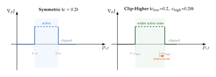
In standard PPO/GRPO, the importance ratio $ρ_{i, t}$ is clipped symmetrically to $[1 - ϵ, 1 + ϵ]$ . This prevents excessively large policy updates. However, Yu et al. observe that symmetric clipping causes entropy collapse: the policy's entropy decreases monotonically during training, and the model converges to a narrow distribution that generates only a few stereotyped responses.

The root cause is an asymmetry in the update dynamics. When a token already has high probability under the current policy:

A positive advantage pushes $ρ_{i, t}$ above $1 + ϵ$ , and the clip prevents further increase: the gradient is zeroed out.
A negative advantage pushes $ρ_{i, t}$ below $1 - ϵ$ , and the clip activates only when the ratio is very small.

The net effect is that high-probability tokens can be suppressed but not amplified, while low-probability tokens (which contribute most to entropy) are clipped on the upside. Over many iterations, the distribution narrows.

Definition 11 (Clip-Higher).

Replace the symmetric clip $[1 - ϵ, 1 + ϵ]$ with an asymmetric clip $[1 - ϵ_{low}, 1 + ϵ_{high}]$ where $ϵ_{high} > ϵ_{low}$ : (CLIP Higher) $\begin{matrix} J_{c l i p - h i g h e r} = \min (ρ_{i, t} {\hat{A}}_{i}, clip (ρ_{i, t}, 1 - ϵ_{low}, 1 + ϵ_{high}) {\hat{A}}_{i}) . \end{matrix}$ In DAPO, $ϵ_{low} = 0.2$ and $ϵ_{high} = 0.28$ .

Proposition 6 (Clip-Higher Prevents Entropy Collapse).

Consider a token with positive advantage ( ${\hat{A}}_{i} > 0$ ). Under symmetric clipping, the gradient $\nabla_{θ} J$ is zeroed when $ρ_{i, t} > 1 + ϵ$ . Under Clip-Higher with $ϵ_{high} > ϵ$ , the gradient remains active for $ρ_{i, t} \in (1 + ϵ, 1 + ϵ_{high}]$ , allowing low-probability tokens (which produce large $ρ_{i, t}$ when their probability increases) to continue increasing. Since entropy $𝖧 (π) = - \sum_{v} π (v) \log π (v)$ increases when probability mass is transferred from high-probability tokens to low-probability tokens, Clip-Higher permits entropy-increasing updates that symmetric clipping blocks.

Symmetric vs. Clip-Higher clipping. The asymmetric upper bound allows low-probability tokens with positive advantage to continue increasing their probability, preventing entropy collapse.

Dynamic Sampling

When all $G$ outputs in a group are correct (or all incorrect), the z-scored advantages are zero (the numerator $r_{i} - \overline{r}$ vanishes for all $i$ ), providing no learning signal. Worse, these degenerate batches still consume compute for sampling and reward evaluation.

Definition 12 (Dynamic Sampling).

After sampling a group of $G$ outputs for prompt $x$ , compute the number of correct outputs $k = \sum_{i} 𝟏 [r_{i} = 1]$ . Discard and resample the group if $k = 0$ or $k = G$ . Only groups satisfying $0 < k < G$ are used for the policy update. Formally, the effective dataset is: $𝒟_{eff} = {(x, o_{1}, \dots, o_{G}) | 0 < \sum_{i = 1}^{G} 𝟏 [r_{i} = 1] < G} .$

Remark 12 (Dynamic Sampling and Difficulty Curriculum).

Dynamic Sampling implicitly creates a difficulty curriculum. Early in training, easy prompts (where $k = G$ ) are filtered out because the model already solves them perfectly. As training progresses and the model improves, harder prompts that previously had $k = 0$ begin producing some correct outputs and enter the training set. This natural curriculum concentrates training signal on prompts at the frontier of the model's capability, neither too easy nor too hard.

Token-Level Loss

Standard GRPO normalizes the loss per sequence: the inner sum over tokens is divided by $| o_{i} |$ , then averaged over the group. This means each sequence contributes equally, regardless of length. Consequently, short sequences have higher per-token gradient magnitude, biasing the policy toward generating shorter outputs.

Definition 13 (Token-Level Loss).

Replace the sequence-level normalization $\frac{1}{G} \sum_{i} \frac{1}{| o_{i} |} \sum_{t} (\dots)$ with a global token normalization: (Token Level LOSS) $\begin{matrix} J_{token} (θ) = \frac{1}{\sum_{i = 1}^{G} | o_{i} |} \sum_{i = 1}^{G} \sum_{t = 1}^{| o_{i} |} [\min (ρ_{i, t} {\hat{A}}_{i}, clip (ρ_{i, t}, 1 - ϵ_{low}, 1 + ϵ_{high}) {\hat{A}}_{i}) - β D_{KL}^{(i, t)}] . \end{matrix}$ Each token contributes equally to the gradient, regardless of the length of the sequence it belongs to.

Overlong Reward Shaping

In practice, generated outputs that exceed the maximum context length $L_{\max}$ are truncated and typically receive zero reward (the truncated output is rarely correct). This creates a sharp cliff in the reward landscape at $L_{\max}$ , which is difficult for the policy to learn from, as the model receives no information about how close it was to producing a valid answer within the length limit.

Definition 14 (Overlong Reward Shaping).

For an output $o_{i}$ that exceeds the length limit $L_{\max}$ , replace the hard zero reward with a soft penalty that increases linearly with the excess length: (Overlong Reward) $\begin{matrix} r_{overlong} (o_{i}) = - \min (1, \max (0, \frac{| o_{i} | - L_{\max}}{L_{cache}})), \end{matrix}$ where $L_{cache}$ is a buffer length (typically $L_{cache} = 512$ tokens). This provides a smooth gradient from $0$ (at $| o_{i} | = L_{\max}$ ) to $- 1$ (at $| o_{i} | = L_{\max} + L_{cache}$ ).

Remark 13 (Gradient of Overlong Reward).

The overlong reward provides a gradient signal proportional to $- 1 / L_{cache}$ for outputs in the range $[L_{\max}, L_{\max} + L_{cache}]$ . This encourages the model to “tighten” its reasoning, finding more concise solution strategies, rather than simply truncating. Without this shaping, the model has no incentive to reduce length until it is already below $L_{\max}$ .

The Full DAPO Algorithm

Combining all four innovations yields the complete DAPO algorithm.

Algorithm 4 (DAPO Training).

Input: Prompt dataset $𝒟$ , policy $π_{θ}$ , reference $π_{ref}$ , reward $r_{ϕ}$ , group size $G$ , clips $ϵ_{low}, ϵ_{high}$ , KL coefficient $β$ , max length $L_{\max}$ , cache $L_{cache}$
for iteration $= 1, 2, \dots$
Sample batch of prompts ${x^{(1)}, \dots, x^{(B)}}$
for each prompt $x^{(j)}$
repeat
Sample $G$ outputs: $o_{1}, \dots, o_{G} \sim π_{θ_{old}} (\cdot | x^{(j)})$
Compute rewards: $r_{i} \leftarrow r_{ϕ} (x^{(j)}, o_{i})$ ; if $| o_{i} | > L_{\max}$ , add $r_{overlong} (o_{i})$
$k \leftarrow \sum_{i} 𝟏 [r_{i} > 0]$ Dynamic Sampling check
until $0 < k < G$
Normalize: ${\hat{A}}_{i} = (r_{i} - \overline{r}) / σ_{r}$
Compute $J_{token} (θ)$ via (Token Level LOSS) with Clip-Higher
Update $θ \leftarrow θ + α \nabla_{θ} J_{token} (θ)$
$θ_{old} \leftarrow θ$

Example 6 (DAPO Ablation on AIME 2024).

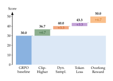
Yu et al. (2025) [11] report a progressive ablation study on the AIME 2024 competition math benchmark, starting from a vanilla GRPO baseline and adding each DAPO innovation:

Configuration	AIME 2024 Score
GRPO baseline	30.0
$+$ Clip-Higher	36.7
$+$ Dynamic Sampling	40.0
$+$ Token-Level Loss	43.3
$+$ Overlong Reward (full DAPO)	50.0

Each innovation provides a meaningful improvement, with the full DAPO system achieving 50.0 on AIME 2024, a 67% relative improvement over the GRPO baseline. Notably, Clip-Higher provides one of the two largest single improvements ( $+$ 6.7 points, matched by Overlong Reward Shaping), confirming that entropy collapse is among the most critical failure modes.

DAPO ablation waterfall chart on AIME 2024. Each innovation adds a meaningful improvement; the shaded region shows the baseline GRPO score.

Alignment for Diffusion Models

The alignment techniques developed in sec:alignment:ppo,sec:alignment:dpo,sec:alignment:grpo were designed for autoregressive language models, where the policy $π_{θ} (y | x)$ is a tractable distribution factorized token by token. But the alignment problem is equally pressing for generative image models. A text-to-image diffusion model may produce photorealistic images, but they may be aesthetically unpleasing, contain artifacts, fail to match the text prompt, or generate unsafe content. Human (or automated) feedback can improve these aspects, if we can formalize the diffusion process as a decision-making problem amenable to RL.

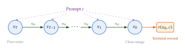
This section shows that the $T$ -step denoising process of a diffusion model can be cast as a Markov Decision Process (MDP), enabling direct application of policy gradient methods. We then survey four complementary alignment approaches: DDPO (RL-based), DRaFT (direct gradient), Diffusion-DPO (preference-based), and ReFL (reward feedback).

Denoising as a Markov Decision Process

Definition 15 (Denoising MDP).

The $T$ -step denoising process of a diffusion model defines an MDP $(𝒮, 𝒜, P, R, T)$ with:

States: $s_{t} = (x_{t}, t, c)$ where $x_{t}$ is the noisy image at step $t$ , $t$ is the timestep, and $c$ is the text conditioning;
Actions: $a_{t} = x_{t - 1}$ , the denoised image at the next step;
Transition: deterministic given the action (the action is the next state's image component);
Policy: $π_{θ} (a_{t} | s_{t}) = p_{θ} (x_{t - 1} | x_{t}, c)$ , the learned denoising distribution;
Reward: $R (s_{0}) = r (x_{0}, c)$ , a scalar reward given only at the final step $t = 0$ , evaluating the quality of the generated image $x_{0}$ with respect to the prompt $c$ .

The denoising process as a Markov Decision Process. Each denoising step is an action, and the reward is given only at the terminal state

x_{0}

Proposition 7 (Exact Log-Probabilities in Gaussian Denoising).

When the denoising policy is Gaussian, $p_{θ} (x_{t - 1} | x_{t}, c) = 𝒩 (x_{t - 1}; μ_{θ} (x_{t}, t, c), σ_{t}^{2} I)$ , the log-probability of each transition is: (Diffusion Logprob) $\begin{matrix} \log p_{θ} (x_{t - 1} | x_{t}, c) = - \frac{d}{2} \log (2 π σ_{t}^{2}) - \frac{‖ x_{t - 1} - μ_{θ} (x_{t}, t, c) ‖^{2}}{2 σ_{t}^{2}}, \end{matrix}$ where $d$ is the dimensionality of $x_{t}$ . This is exact and differentiable; no approximation is needed, unlike the intractable $\log p_{θ} (x_{0})$ of the full generative model.

Proof.

This follows directly from the density of a multivariate Gaussian with diagonal covariance $σ_{t}^{2} I$ .

∎

DDPO: Denoising Diffusion Policy Optimization

Black et al. (2024) [19] propose DDPO, applying policy gradient methods directly to the denoising MDP.

The policy gradient for the denoising MDP is: (DDPO Gradient) $\begin{matrix} \nabla_{θ} J = 𝔼 [r (x_{0}, c) \sum_{t = 1}^{T} \nabla_{θ} \log p_{θ} (x_{t - 1} | x_{t}, c)] . \end{matrix}$ This is a standard REINFORCE gradient applied to the $T$ -step trajectory. Black et al. propose two variants:

DDPO-SF (score function): Directly applies (DDPO Gradient) with a learned baseline $b (c)$ to reduce variance: $\nabla_{θ} J \approx 𝔼 [(r (x_{0}, c) - b (c)) \sum_{t} \nabla_{θ} \log p_{θ} (x_{t - 1} | x_{t}, c)]$ .
DDPO-IS (importance sampling): Uses a PPO-style clipped objective with importance ratios: (DDPO IS) $\begin{matrix} J_{D D P O - I S} = 𝔼 [\sum_{t = 1}^{T} \min (ρ_{t} \hat{A}, clip (ρ_{t}, 1 - ϵ, 1 + ϵ) \hat{A})], \end{matrix}$ where $ρ_{t} = p_{θ} (x_{t - 1} | x_{t}, c) / p_{θ_{old}} (x_{t - 1} | x_{t}, c)$ and $\hat{A} = r (x_{0}, c) - b (c)$ .

Remark 14 (Variance Scales with $T$ ).

The REINFORCE gradient in (DDPO Gradient) has variance that scales linearly with the number of denoising steps $T$ , since the trajectory length is $T$ . With typical values of $T = 50$ – $1000$ , this can be substantial. DDPO-IS mitigates this through the clipping mechanism, and practical implementations often use $T = 50$ (DDIM sampling) rather than $T = 1000$ (DDPM).

DRaFT: Direct Reward Fine-Tuning

When the reward function $r$ is differentiable with respect to the generated image $x_{0}$ (e.g., a neural network aesthetic scorer or CLIP similarity), we can bypass the high-variance REINFORCE estimator entirely and backpropagate the reward gradient directly through the denoising chain.

Definition 16 (DRaFT Objective).

Given a differentiable reward $r (x_{0}, c)$ , the DRaFT objective [12] is simply: (Draft) $\begin{matrix} ℒ_{DRaFT} (θ) = - 𝔼_{x_{T} \sim 𝒩 (0, I), c \sim 𝒟} [r ({Denoise}_{θ} (x_{T}, c), c)], \end{matrix}$ where ${Denoise}_{θ} (x_{T}, c)$ denotes the full $T$ -step deterministic (DDIM) denoising chain from $x_{T}$ to $x_{0}$ .

The gradient $\nabla_{θ} ℒ_{DRaFT}$ is computed by backpropagating through all $T$ denoising steps. For a typical diffusion model with $T = 50$ steps and hundreds of millions of parameters, this requires enormous memory. DRaFT addresses this in two ways:

DRaFT- $K$ : Backpropagate through only the last $K$ denoising steps (typically $K = 1$ or $K = 5$ ), treating the first $T - K$ steps as frozen. This reduces memory by a factor of $T / K$ at the cost of a biased gradient.
LoRA: Apply LoRA (Parameter-Efficient Fine-Tuning: LoRA) to the diffusion model's U-Net, reducing the number of trainable parameters and the memory footprint of gradient computation.

Remark 15 (DRaFT-1 Approximation Quality).

Clark et al. (2024) show empirically that DRaFT-1 (backprop through only the final denoising step) achieves 80–90% of the reward improvement of full-chain DRaFT, while using $50 \times$ less memory. This is because the final denoising step has the most direct influence on the pixel-level content of $x_{0}$ ; earlier steps primarily determine the coarse structure, which is less sensitive to small parameter changes.

Diffusion-DPO: Preference Learning for Diffusion

Wallace et al. (2024) [13] adapt DPO (Direct Preference Optimization) to diffusion models. The key challenge is that DPO requires log-likelihoods $\log π_{θ} (y | x)$ , but for diffusion models the marginal likelihood $\log p_{θ} (x_{0} | c)$ is intractable.

The solution uses the evidence lower bound (ELBO) as a proxy. Recall that for a diffusion model, the ELBO decomposes into a sum of per-step terms: (Diffusion ELBO) $\begin{matrix} \log p_{θ} (x_{0} | c) \geq ELBO = - \sum_{t = 1}^{T} 𝔼_{q (x_{t} | x_{0})} [D_{KL} [q (x_{t - 1} | x_{t}, x_{0}) ‖ p_{θ} (x_{t - 1} | x_{t}, c)]] + C, \end{matrix}$ where $C$ is a constant independent of $θ$ .

Definition 17 (Diffusion-DPO Loss).

Given preference pairs $(c, x_{0}^{w}, x_{0}^{l})$ where $x_{0}^{w}$ is preferred over $x_{0}^{l}$ , the Diffusion-DPO loss [13] is: (Diffusion DPO) $\begin{matrix} ℒ_{Diff-DPO} = - 𝔼 [\log σ (- β T Δ ℒ)], \end{matrix}$ where $Δ ℒ$ is the difference in per-step denoising losses: (Diffusion DPO Delta) $\begin{matrix} Δ ℒ & = (‖ 𝝐 - 𝝐_{θ} (x_{t}^{w}, t, c) ‖^{2} - ‖ 𝝐 - 𝝐_{ref} (x_{t}^{w}, t, c) ‖^{2}) \\ - (‖ 𝝐 - 𝝐_{θ} (x_{t}^{l}, t, c) ‖^{2} - ‖ 𝝐 - 𝝐_{ref} (x_{t}^{l}, t, c) ‖^{2}), \end{matrix}$ with $t$ sampled uniformly from ${1, \dots, T}$ , $𝝐 \sim 𝒩 (0, I)$ , and $x_{t}^{w}, x_{t}^{l}$ obtained by adding noise to $x_{0}^{w}, x_{0}^{l}$ according to the forward diffusion schedule.

Insight.

Diffusion-DPO is a single-step loss. Despite the diffusion model having $T$ denoising steps, the Diffusion-DPO loss evaluates at a single randomly sampled timestep $t$ , just like standard diffusion training. This makes it as computationally efficient as regular fine-tuning; no multi-step sampling or trajectory rollout is needed. The factor of $T$ in (Diffusion DPO) compensates for the single-step approximation to the full ELBO.

Example 7 (Aligning Stable Diffusion with Aesthetics).

Wallace et al. (2024) [13] align Stable Diffusion XL using Diffusion-DPO with the Pick-a-Pic dataset of human preference pairs. The aligned model achieves a 69% win rate against the base model in human evaluations of visual quality, while maintaining text-image alignment. DDPO achieves similar win rates but requires online sampling during training, making it approximately $5 \times$ more expensive.

ReFL: Reward Feedback Learning

Xu et al. (2023) [20] propose a simpler approach when a differentiable reward model (ImageReward) is available: simply backpropagate the reward signal into the later denoising steps.

Definition 18 (ReFL Objective).

The ReFL loss fine-tunes only the last $K$ denoising steps: (REFL) $\begin{matrix} ℒ_{ReFL} (θ) = - 𝔼_{x_{K} \sim p_{θ}^{frozen}} [r_{IR} ({\hat{x}}_{0} (x_{K}, θ), c)], \end{matrix}$ where ${\hat{x}}_{0} (x_{K}, θ)$ is the predicted clean image from step $K$ using a one-step approximation, and $r_{IR}$ is the ImageReward model.

Remark 16 (ReFL vs. DRaFT).

ReFL is essentially a special case of DRaFT- $K$ using ImageReward as the reward function. The key contribution is the ImageReward model itself: a BLIP-based model fine-tuned on 137K human preference annotations that correlates well with human judgments of text-image alignment and aesthetic quality.

Diffusion Alignment Taxonomy

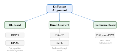
Taxonomy of diffusion model alignment methods.

Method	Approach	Reward Type	Online Sampling	Multi-Step Backprop	Data
DDPO	Policy gradient	Any (black-box)	Yes	No	None (online)
DRaFT	Direct gradient	Differentiable	No	Yes ( $K$ steps)	None
Diffusion-DPO	Preference	None needed	No	No	Preference pairs
ReFL	Direct gradient	Differentiable	No	Yes ( $K$ steps)	None

Comparison of diffusion alignment methods.

Connections and Synthesis

Having developed the mathematical foundations of six alignment methods (PPO, DPO, GRPO, DAPO, DDPO, Diffusion-DPO) and two direct-gradient methods (DRaFT, ReFL), we now step back and identify the unifying themes.

A Unified Framework

Definition 19 (Unified Alignment Objective).

Every alignment method discussed in this chapter can be viewed as an instance of the constrained optimization problem: (Unified) $\begin{matrix} \max_{π} ℛ (π) - β 𝒞 (π, π_{ref}), \end{matrix}$ where $ℛ (π)$ is a reward functional measuring alignment quality and $𝒞 (π, π_{ref})$ is a constraint functional measuring deviation from the reference policy.

The methods differ in how they instantiate $ℛ$ , how they handle the constraint $𝒞$ , and whether optimization is performed online (with sampling) or offline (on a fixed dataset):

Method	Models	Online?	Gradient	Memory	Best For
PPO (RLHF)	4	Yes	Policy gradient	Very high	General alignment
DPO	2	No	Supervised	Low	Preference-rich data
GRPO	3	Yes	Policy gradient	High	Verifiable tasks
DAPO	3	Yes	Policy gradient	High	Large-scale math/code
DDPO	2	Yes	Policy gradient	Moderate	Image alignment (any reward)
Diff-DPO	2	No	Supervised	Low	Image alignment (preference data)
DRaFT	1	No	Direct (backprop)	Moderate	Image alignment (differentiable reward)
ReFL	1	No	Direct (backprop)	Low	Image alignment (ImageReward)

Unified comparison of alignment methods. “Models” counts the number of neural networks held in GPU memory simultaneously.

The Alignment Spectrum

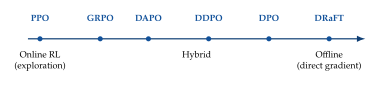
The methods in this chapter can be arranged along a spectrum from fully online RL to fully offline supervised learning:

Key Idea.

No single method dominates. The choice of alignment method depends on three factors:

Reward verifiability: For tasks with automatic verifiers (math, code), GRPO/DAPO excel because they can leverage binary correctness signals. For tasks requiring human judgment (creative writing, helpfulness), PPO or DPO with preference data is more appropriate.
Data availability: DPO requires a static dataset of preference pairs; PPO/GRPO generate their own data online. If collecting preference data is cheap, DPO is simpler; if expensive, online methods amortize the cost.
Compute budget: PPO requires 4 models in memory; GRPO eliminates the critic; DPO requires only 2. At frontier scale (100B+ parameters), memory constraints often dictate the method.

Historical Timeline

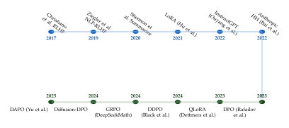
Historical timeline of alignment research. The field has evolved from RL-based methods (top row) toward simpler, more efficient approaches (bottom row).

Historical Note.

The alignment research timeline reveals a clear trend toward simplification. The original RLHF pipeline (Christiano et al., 2017) required a separate reward model and a full RL training loop. InstructGPT (2022) made this practical at scale but still needed four neural networks. DPO (2023) eliminated the reward model and RL loop entirely. GRPO (2024) kept the RL formulation but eliminated the critic. DAPO (2025) refined GRPO with engineering innovations for scale. Meanwhile, diffusion alignment followed a parallel trajectory: from DDPO (RL-based) to Diffusion-DPO (direct preference) and DRaFT/ReFL (direct gradient). The field is converging toward methods that are simpler, more memory-efficient, and require less infrastructure, while maintaining or improving alignment quality.

Exercises

Exercise 1 (SFT Loss Derivation).

Show that the SFT objective $ℒ_{SFT} (θ) = - \frac{1}{N} \sum_{i = 1}^{N} \sum_{t = 1}^{T_{i}} \log π_{θ} (y_{t}^{(i)} | x^{(i)}, y_{< t}^{(i)})$ is equivalent to minimizing the KL divergence $D_{KL} [{\hat{p}}_{data} ‖ π_{θ}]$ where ${\hat{p}}_{data}$ is the empirical distribution of demonstration sequences, up to a constant independent of $θ$ .

Exercise 2 (LoRA Parameter Count).

Consider LLaMA-7B, which has 32 transformer layers, each containing attention projections $W_{Q}, W_{K}, W_{V}, W_{O} \in ℝ^{4096 \times 4096}$ and MLP projections $W_{gate}, W_{up} \in ℝ^{4096 \times 11008}$ and $W_{down} \in ℝ^{11008 \times 4096}$ .

How many total parameters does the model have in these weight matrices alone?
If LoRA with rank $r = 8$ is applied to $W_{Q}$ and $W_{V}$ only, how many trainable parameters are added? What fraction of the full parameter count is this?
Repeat (b) for rank $r = 64$ applied to all seven weight matrices. At what rank does LoRA training cost exceed 1% of full fine-tuning?

Exercise 3 (Bradley–Terry MLE).

Derive the Bradley–Terry MLE explicitly. Given $N$ preference pairs $(y_{w}^{(i)}, y_{l}^{(i)})$ for a fixed prompt $x$ , and a parametric reward function $r_{ϕ} (x, y)$ , show that the negative log-likelihood $ℒ (ϕ) = - \sum_{i = 1}^{N} \log σ (r_{ϕ} (x, y_{w}^{(i)}) - r_{ϕ} (x, y_{l}^{(i)}))$ is convex in the reward differences $δ_{i} = r_{ϕ} (x, y_{w}^{(i)}) - r_{ϕ} (x, y_{l}^{(i)})$ .

Exercise 4 (Reward Identifiability).

Prove that the reward function under the Bradley–Terry model is identifiable only up to a prompt-dependent constant. Specifically, show that if $r (x, y)$ satisfies $p (y_{w} ≻ y_{l} | x) = σ (r (x, y_{w}) - r (x, y_{l}))$ for all pairs, then $r^{'} (x, y) = r (x, y) + f (x)$ for any function $f$ satisfies the same equations. Conversely, show that any two solutions must differ by such an additive function.

Exercise 5 (DPO Reparameterization from Scratch).

Starting from the KL-constrained objective $\max_{π} 𝔼 [r (x, y)] - β D_{KL} [π ‖ π_{ref}]$ :

Derive the optimal policy $π^{*} (y | x) \propto π_{ref} (y | x) \exp (r (x, y) / β)$ .
Invert this to express the reward as $r (x, y) = β \log \frac{π^{*} (y | x)}{π_{ref} (y | x)} + β \log Z (x)$ .
Substitute into the Bradley–Terry model and show that $Z (x)$ cancels.
Write the resulting DPO loss explicitly.
Verify that $\nabla_{θ} ℒ_{DPO} = 0$ when $π_{θ} = π^{*}$ .

Exercise 6 (DPO Gradient Analysis).

Compute the gradient of the DPO loss with respect to $θ$ : $\nabla_{θ} ℒ_{DPO} = - β 𝔼 [σ ({\hat{r}}_{l} - {\hat{r}}_{w}) (\nabla_{θ} \log π_{θ} (y_{w} | x) - \nabla_{θ} \log π_{θ} (y_{l} | x))],$ where ${\hat{r}}_{y} = β \log \frac{π_{θ} (y | x)}{π_{ref} (y | x)}$ .

Show that the sigmoid weight $σ ({\hat{r}}_{l} - {\hat{r}}_{w})$ is large when the model assigns higher implicit reward to the losing response, interpreting this as “hard example mining.”
What happens to the gradient magnitude as training progresses and the model correctly ranks most preference pairs?
Compare this to the PPO gradient, which weights updates by the advantage $\hat{A}$ . Under what conditions are the two gradients similar?

Exercise 7 (DPO–RLHF Equivalence).

Prove that in the infinite-data, infinite-capacity regime, the DPO and RLHF solutions coincide. Specifically:

Show that if $π_{θ}$ is the global minimizer of the DPO loss (over all policies), then $π_{θ}$ is the optimal policy of the KL-constrained RLHF objective.
Show that if the preference data is generated according to the Bradley–Terry model with a ground-truth reward $r^{*}$ , then the implicit DPO reward $\hat{r} (x, y) = β \log \frac{π_{θ} (y | x)}{π_{ref} (y | x)}$ recovers $r^{*} (x, y)$ up to a prompt-dependent constant.

Exercise 8 (GRPO Advantage Variance).

Analyze the variance of the GRPO advantage estimator.

For a fixed prompt, let $r_{1}, \dots, r_{G} \overset{iid}{\sim} p_{r}$ be i.i.d. rewards. Compute $𝖵ar [{\hat{A}}_{1}]$ in terms of the moments of $p_{r}$ and the group size $G$ .
Show that $𝖵ar [{\hat{A}}_{1}] \to 1$ as $G \to \infty$ (since the z-score has unit variance in the limit).
For binary rewards with success probability $p$ , find the group size $G^{*}$ that minimizes the coefficient of variation of the advantage. How does $G^{*}$ depend on $p$ ?

Exercise 9 (PPO vs. GRPO Memory).

Consider a transformer with $L$ layers, hidden dimension $d$ , and $P$ total parameters. Assume Adam optimization (2 states per parameter) and 16-bit mixed precision.

Compute the GPU memory required for PPO training: policy ( $P$ params + Adam states), critic ( $P$ params + Adam states), reward model ( $P$ params, frozen), reference ( $P$ params, frozen).
Compute the memory for GRPO (no critic).
For $P = 7 \times 10^{9}$ , compute the memory savings in gigabytes. At what model size does the saving exceed the capacity of a single A100 (80,GB)?

Exercise 10 (Clip-Higher Entropy Analysis).

Consider a vocabulary of size $V$ and a policy $π_{θ}$ over this vocabulary. Suppose token $v$ has $π_{θ} (v) = δ ≪ 1 / V$ and positive advantage $\hat{A} > 0$ .

Show that after one gradient step with symmetric clipping $ϵ$ , the importance ratio for token $v$ is clipped at $1 + ϵ$ when $δ$ is small enough.
With Clip-Higher ( $ϵ_{high} > ϵ$ ), compute the additional probability mass that can be transferred to token $v$ per update step.
Argue that the entropy $𝖧 (π_{θ})$ is increasing in the probability of low-probability tokens. Conclude that Clip-Higher permits entropy-increasing updates.

Exercise 11 (Dynamic Sampling Probability).

Suppose the policy produces correct outputs with probability $p$ for a given prompt, independently across the group.

Compute the probability that a group of size $G$ passes the Dynamic Sampling filter (i.e., $0 < k < G$ ).
For $G = 16$ , plot this probability as a function of $p$ . At what values of $p$ is filtering most likely to reject?
Compute the expected number of sampling attempts before passing the filter.
How does Dynamic Sampling affect the effective training distribution? Show that prompts with $p \approx 0$ or $p \approx 1$ are underrepresented relative to prompts with $p \approx 0.5$ .

Exercise 12 (Overlong Reward Gradient).

Consider the overlong reward shaping from Definition 14.

Compute $\frac{\partial r_{overlong}}{\partial | o_{i} |}$ for outputs in the three regimes: $| o_{i} | < L_{\max}$ , $L_{\max} \leq | o_{i} | \leq L_{\max} + L_{cache}$ , and $| o_{i} | > L_{\max} + L_{cache}$ .
Show that the gradient magnitude in the middle regime is $1 / L_{cache}$ . What is the effect of increasing $L_{cache}$ ?
Compare this to a hard threshold reward (0 for $| o_{i} | > L_{\max}$ , full reward otherwise) in terms of the gradient signal available at length $L_{\max} + 1$ .

Exercise 13 (Diffusion MDP Formalization).

Formalize the denoising MDP of Definition 15 rigorously.

Define the state space $𝒮$ , action space $𝒜$ , and transition kernel $P$ precisely.
Show that the trajectory probability is $p_{θ} (τ) = p (x_{T}) \prod_{t = 1}^{T} p_{θ} (x_{t - 1} | x_{t}, c)$ .
Derive the policy gradient $\nabla_{θ} J = 𝔼 [r (x_{0}, c) \sum_{t = 1}^{T} \nabla_{θ} \log p_{θ} (x_{t - 1} | x_{t}, c)]$ from the standard REINFORCE theorem.
Compute the variance of this estimator as a function of $T$ and the reward variance.

Exercise 14 (DDPO Variance vs. Denoising Steps).

The REINFORCE gradient for the denoising MDP has the form $g = r (x_{0}, c) \sum_{t = 1}^{T} \nabla_{θ} \log p_{θ} (x_{t - 1} | x_{t}, c)$ .

Assuming the per-step score functions $\nabla_{θ} \log p_{θ} (x_{t - 1} | x_{t}, c)$ are independent with variance $σ_{s}^{2}$ (a simplifying assumption), show that $𝖵ar [g] = T σ_{s}^{2} 𝖵ar [r] + T^{2} σ_{s}^{2} 𝔼 {[r]}^{2}$ (approximately).
Using DDIM with $T^{'} ≪ T$ steps, how does the variance change? Argue that reducing $T^{'}$ by a factor of $k$ reduces variance by approximately the same factor.
Why does DDPO-IS (PPO-style clipping) further reduce variance compared to DDPO-SF (REINFORCE)?

Exercise 15 (DRaFT- $K$ Gradient Approximation).

In DRaFT- $K$ , we backpropagate through only the last $K$ steps.

Write the DRaFT- $K$ gradient as $\nabla_{θ} ℒ_{K} = - \nabla_{x_{K}} r ({\hat{x}}_{0}) \cdot \frac{\partial {\hat{x}}_{0}}{\partial x_{K}} \cdot \frac{\partial x_{K}}{\partial θ}$ (chain rule through $K$ steps).
Show that DRaFT- $T$ (full chain) gives the exact gradient, while DRaFT-1 is a biased approximation.
Assuming the Jacobians $‖ \partial x_{t - 1} / \partial x_{t} ‖ \leq ρ < 1$ (a contraction), bound the approximation error $‖ \nabla_{θ} ℒ_{T} - \nabla_{θ} ℒ_{K} ‖$ in terms of $ρ$ and $T - K$ .
For Stable Diffusion with $T = 50$ and a typical contraction factor $ρ \approx 0.95$ , at what $K$ is the approximation error below 10% of the full gradient norm?

Exercise 16 (Diffusion-DPO ELBO Derivation).

Derive the Diffusion-DPO loss from first principles.

Starting from the standard DPO loss $ℒ = - \log σ (β \log \frac{π_{θ} (x_{0}^{w} | c)}{π_{ref} (x_{0}^{w} | c)} - β \log \frac{π_{θ} (x_{0}^{l} | c)}{π_{ref} (x_{0}^{l} | c)})$ , substitute the ELBO approximation for $\log π_{θ} (x_{0} | c)$ .
Show that the ELBO difference simplifies to a sum of per-step denoising loss differences.
Argue that sampling a single timestep $t$ and multiplying by $T$ gives an unbiased estimator of the full ELBO difference.
Write out the final single-step loss and verify it matches (Diffusion DPO).

Exercise 17 (LoRA Rank vs. Accuracy).

The LoRA update is $Δ W = B A$ where $B \in ℝ^{d \times r}$ and $A \in ℝ^{r \times k}$ .

Show that $rank (Δ W) \leq r$ .
If the true optimal update $Δ W^{*} = W^{*} - W_{0}$ has rank $R > r$ , bound the approximation error $‖ B A - Δ W^{*} ‖_{F}$ in terms of the singular values of $Δ W^{*}$ (hint: Eckart–Young theorem).
Discuss the trade-off: increasing $r$ reduces approximation error but increases memory and risks overfitting. When is $r = 8$ likely sufficient vs. when is $r = 64$ needed?

Exercise 18 (KL Penalty Sensitivity).

Consider the KL-constrained objective $J (π) = 𝔼_{π} [r (x, y)] - β D_{KL} [π ‖ π_{ref}]$ .

Show that $\frac{\partial J^{*}}{\partial β} = - D_{KL} [π^{*} ‖ π_{ref}]$ where $J^{*}$ is the optimal value and $π^{*}$ the optimal policy (envelope theorem).
Conclude that increasing $β$ always decreases the optimal reward.
For the DPO loss, show that the implicit KL constraint is controlled by $β$ . What happens as $β \to 0$ and $β \to \infty$ ?
Design an experiment to select $β$ optimally for a specific task. What metric would you use?

Exercise 19 (Designing an Alignment Pipeline).

You are tasked with aligning a 13B-parameter language model for code generation. The model should produce correct, efficient, and well-documented Python code. You have access to:

A training dataset of 50K coding problems with reference solutions;
An automated test suite that can verify correctness;
8 NVIDIA A100 GPUs (80,GB each);
A budget of 500 GPU-hours.

Which alignment method(s) would you choose? Justify based on the properties of the task and available resources.
Design the reward function. Would you use binary (pass/fail) rewards or a more nuanced scoring?
Estimate the memory requirements for your chosen method. Does it fit in 8 $\times$ 80,GB with appropriate parallelism?
Describe how you would monitor for reward hacking.

Exercise 20 (Open Problem: Optimal $β$ Schedule).

In all alignment methods, $β$ is typically fixed throughout training. Investigate whether a $β$ schedule could improve results.

Argue intuitively why starting with small $β$ (aggressive optimization) and increasing it (conservative fine-tuning) might be beneficial.
Conversely, argue why starting with large $β$ (exploration near $π_{ref}$ ) and decreasing it (exploitation) could also work.
Design a simple $β$ schedule (e.g., linear, cosine, step) and describe how you would evaluate it experimentally.
This is an open research problem. What theoretical tools (e.g., regret bounds, convergence rates) might help determine the optimal schedule?

References

Deep Reinforcement Learning from Human Preferences

Paul F Christiano, Jan Leike, Tom Brown, Miljan Martic, Shane Legg, Dario Amodei

Advances in Neural Information Processing Systems, vol. 30 · 2017

BibTeX

@article{christiano2017deep,
  title={Deep Reinforcement Learning from Human Preferences},
  author={Christiano, Paul F and Leike, Jan and Brown, Tom and Martic, Miljan and Legg, Shane and Amodei, Dario},
  journal={Advances in Neural Information Processing Systems},
  volume={30},
  year={2017}
}

Journal article

Fine-Tuning Language Models from Human Preferences

Daniel M Ziegler, Nisan Stiennon, Jeffrey Wu, Tom B Brown, Alec Radford, Dario Amodei, Paul Christiano, Geoffrey Irving

arXiv preprint arXiv:1909.08593 · 2019

BibTeX

@article{ziegler2019fine,
  title={Fine-Tuning Language Models from Human Preferences},
  author={Ziegler, Daniel M and Stiennon, Nisan and Wu, Jeffrey and Brown, Tom B and Radford, Alec and Amodei, Dario and Christiano, Paul and Irving, Geoffrey},
  journal={arXiv preprint arXiv:1909.08593},
  year={2019}
}

Journal article

Learning to Summarize with Human Feedback

Nisan Stiennon, Long Ouyang, Jeffrey Wu, Daniel Ziegler, Ryan Lowe, Chelsea Voss, Alec Radford, Dario Amodei, et al.

Advances in Neural Information Processing Systems, vol. 33, pp. 3008-3021 · 2020

BibTeX

@article{stiennon2020learning,
  title={Learning to Summarize with Human Feedback},
  author={Stiennon, Nisan and Ouyang, Long and Wu, Jeffrey and Ziegler, Daniel and Lowe, Ryan and Voss, Chelsea and Radford, Alec and Amodei, Dario and Christiano, Paul F},
  journal={Advances in Neural Information Processing Systems},
  volume={33},
  pages={3008--3021},
  year={2020}
}

Journal article

Training Language Models to Follow Instructions with Human Feedback

Long Ouyang, Jeffrey Wu, Xu Jiang, Diogo Almeida, Carroll Wainwright, Pamela Mishkin, Chong Zhang, Sandhini Agarwal, et al.

Advances in Neural Information Processing Systems, vol. 35, pp. 27730-27744 · 2022

BibTeX

@article{ouyang2022training,
  title={Training Language Models to Follow Instructions with Human Feedback},
  author={Ouyang, Long and Wu, Jeffrey and Jiang, Xu and Almeida, Diogo and Wainwright, Carroll and Mishkin, Pamela and Zhang, Chong and Agarwal, Sandhini and Slama, Katarina and Ray, Alex and others},
  journal={Advances in Neural Information Processing Systems},
  volume={35},
  pages={27730--27744},
  year={2022}
}

Journal article

Direct Preference Optimization: Your Language Model is Secretly a Reward Model

Rafael Rafailov, Archit Sharma, Eric Mitchell, Stefano Ermon, Christopher D Manning, Chelsea Finn

Advances in Neural Information Processing Systems, vol. 36 · 2023

BibTeX

@article{rafailov2023direct,
  title={Direct Preference Optimization: Your Language Model is Secretly a Reward Model},
  author={Rafailov, Rafael and Sharma, Archit and Mitchell, Eric and Ermon, Stefano and Manning, Christopher D and Finn, Chelsea},
  journal={Advances in Neural Information Processing Systems},
  volume={36},
  year={2023}
}

Journal article

QLoRA: Efficient Finetuning of Quantized Language Models

Tim Dettmers, Artidoro Pagnoni, Ari Holtzman, Luke Zettlemoyer

Advances in Neural Information Processing Systems, vol. 36 · 2023

BibTeX

@article{dettmers2023qlora,
  title={{QLoRA}: Efficient Finetuning of Quantized Language Models},
  author={Dettmers, Tim and Pagnoni, Artidoro and Holtzman, Ari and Zettlemoyer, Luke},
  journal={Advances in Neural Information Processing Systems},
  volume={36},
  year={2023}
}

Journal article

Intrinsic Dimensionality Explains the Effectiveness of Language Model Fine-Tuning

Armen Aghajanyan, Sonal Gupta, Luke Zettlemoyer

arXiv preprint arXiv:2012.13255 · 2021

BibTeX

@article{aghajanyan2021intrinsic,
  title={Intrinsic Dimensionality Explains the Effectiveness of Language Model Fine-Tuning},
  author={Aghajanyan, Armen and Gupta, Sonal and Zettlemoyer, Luke},
  journal={arXiv preprint arXiv:2012.13255},
  year={2021}
}

Journal article

S-LoRA: Serving Thousands of Concurrent LoRA Adapters

Ying Sheng, Shiyi Cao, Dacheng Li, Coleman Hooper, Nicholas Lee, Shuo Yang, Christopher Chou, Banghua Zhu, et al.

arXiv preprint arXiv:2311.03285 · 2024

BibTeX

@article{sheng2024slora,
  title={{S-LoRA}: Serving Thousands of Concurrent {LoRA} Adapters},
  author={Sheng, Ying and Cao, Shiyi and Li, Dacheng and Hooper, Coleman and Lee, Nicholas and Yang, Shuo and Chou, Christopher and Zhu, Banghua and Zheng, Lianmin and Keutzer, Kurt and Gonzalez, Joseph E and Stoica, Ion},
  journal={arXiv preprint arXiv:2311.03285},
  year={2024}
}

Journal article

Scaling Laws for Reward Model Overoptimization

Leo Gao, John Schulman, Jacob Hilton

arXiv preprint arXiv:2210.10760 · 2023

BibTeX

@article{gao2023scaling,
  title={Scaling Laws for Reward Model Overoptimization},
  author={Gao, Leo and Schulman, John and Hilton, Jacob},
  journal={arXiv preprint arXiv:2210.10760},
  year={2023}
}

Journal article

DeepSeek-R1: Incentivizing Reasoning Capability in LLMs via Reinforcement Learning

DeepSeek-AI

arXiv preprint arXiv:2501.12948 · 2025

BibTeX

@article{deepseekr1,
  title={{DeepSeek-R1}: Incentivizing Reasoning Capability in {LLMs} via Reinforcement Learning},
  author={{DeepSeek-AI}},
  journal={arXiv preprint arXiv:2501.12948},
  year={2025}
}

Journal article

DAPO: An Open-Source LLM Reinforcement Learning System at Scale

Qiying Yu, others

arXiv preprint arXiv:2503.14476 · 2025

BibTeX

@article{yu2025dapo,
  title={{DAPO}: An Open-Source {LLM} Reinforcement Learning System at Scale},
  author={Yu, Qiying and others},
  journal={arXiv preprint arXiv:2503.14476},
  year={2025}
}

Journal article

Directly Fine-Tuning Diffusion Models on Differentiable Rewards

Kevin Clark, Paul Vicol, Kevin Swersky, David J Fleet

International Conference on Learning Representations · 2024

BibTeX

@article{clark2024directly,
  title={Directly Fine-Tuning Diffusion Models on Differentiable Rewards},
  author={Clark, Kevin and Vicol, Paul and Swersky, Kevin and Fleet, David J},
  journal={International Conference on Learning Representations},
  year={2024}
}

Journal article

Diffusion Model Alignment Using Direct Preference Optimization

Bram Wallace, Meihua Dang, Rafael Rafailov, Linqi Zhou, Aaron Lou, Senthil Purber, Stefano Ermon, Caiming Xiong, et al.

Conference on Computer Vision and Pattern Recognition · 2024

BibTeX

@article{wallace2024diffusion,
  title={Diffusion Model Alignment Using Direct Preference Optimization},
  author={Wallace, Bram and Dang, Meihua and Rafailov, Rafael and Zhou, Linqi and Lou, Aaron and Purber, Senthil and Ermon, Stefano and Xiong, Caiming and Joty, Shafiq and Naik, Nikhil},
  journal={Conference on Computer Vision and Pattern Recognition},
  year={2024}
}

Journal article

On the Dangers of Stochastic Parrots: Can Language Models Be Too Big?

Emily M Bender, Timnit Gebru, Angelina McMillan-Major, Shmargaret Shmitchell

Proceedings of the ACM Conference on Fairness, Accountability, and Transparency (FAccT) · 2021

BibTeX

@inproceedings{bender2021dangers,
  title={On the Dangers of Stochastic Parrots: Can Language Models Be Too Big?},
  author={Bender, Emily M and Gebru, Timnit and McMillan-Major, Angelina and Shmitchell, Shmargaret},
  booktitle={Proceedings of the ACM Conference on Fairness, Accountability, and Transparency (FAccT)},
  year={2021}
}

Conference paper

Stanford Alpaca: An Instruction-Following LLaMA Model

Rohan Taori, Ishaan Gulrajani, Tianyi Zhang, Yann Dubois, Xuechen Li, Carlos Guestrin, Percy Liang, Tatsunori B Hashimoto

GitHub repository · 2023

BibTeX

@article{taori2023stanford,
  title={Stanford {Alpaca}: An Instruction-Following {LLaMA} Model},
  author={Taori, Rohan and Gulrajani, Ishaan and Zhang, Tianyi and Dubois, Yann and Li, Xuechen and Guestrin, Carlos and Liang, Percy and Hashimoto, Tatsunori B},
  journal={GitHub repository},
  year={2023}
}

Journal article

LoRA: Low-Rank Adaptation of Large Language Models

Edward J Hu, Yelong Shen, Phillip Wallis, Zeyuan Allen-Zhu, Yuanzhi Li, Shean Wang, Lu Wang, Weizhu Chen

International Conference on Learning Representations · 2022

BibTeX

@article{hu2022lora,
  title={{LoRA}: Low-Rank Adaptation of Large Language Models},
  author={Hu, Edward J and Shen, Yelong and Wallis, Phillip and Allen-Zhu, Zeyuan and Li, Yuanzhi and Wang, Shean and Wang, Lu and Chen, Weizhu},
  journal={International Conference on Learning Representations},
  year={2022}
}

Journal article

Rank Analysis of Incomplete Block Designs: I. The Method of Paired Comparisons

Ralph Allan Bradley, Milton E Terry

Biometrika, vol. 39, no. 3/4, pp. 324-345 · 1952

BibTeX

@article{bradley1952rank,
  title={Rank Analysis of Incomplete Block Designs: {I}. The Method of Paired Comparisons},
  author={Bradley, Ralph Allan and Terry, Milton E},
  journal={Biometrika},
  volume={39},
  number={3/4},
  pages={324--345},
  year={1952}
}

Journal article

DeepSeekMath: Pushing the Limits of Mathematical Reasoning in Open Language Models

Zhihong Shao, Peiyi Wang, Qihao Zhu, Runxin Xu, Junxiao Song, Mingchuan Zhang, Y.K. Li, Y. Wu, et al.

arXiv preprint arXiv:2402.03300 · 2024

BibTeX

@article{shao2024deepseekmath,
  title={{DeepSeekMath}: Pushing the Limits of Mathematical Reasoning in Open Language Models},
  author={Shao, Zhihong and Wang, Peiyi and Zhu, Qihao and Xu, Runxin and Song, Junxiao and Zhang, Mingchuan and Li, Y.K. and Wu, Y. and Guo, Daya},
  journal={arXiv preprint arXiv:2402.03300},
  year={2024}
}

Journal article

Training Diffusion Models with Reinforcement Learning

Kevin Black, Michael Janner, Yilun Du, Ilya Kostrikov, Sergey Levine

International Conference on Learning Representations · 2024

BibTeX

@article{black2024training,
  title={Training Diffusion Models with Reinforcement Learning},
  author={Black, Kevin and Janner, Michael and Du, Yilun and Kostrikov, Ilya and Levine, Sergey},
  journal={International Conference on Learning Representations},
  year={2024}
}

Journal article

ImageReward: Learning and Evaluating Human Preferences for Text-to-Image Generation

Jiazheng Xu, Xiao Liu, Yuchen Wu, Yuxuan Tong, Qinkai Li, Ming Ding, Jie Tang, Yuxiao Dong

Advances in Neural Information Processing Systems, vol. 36 · 2023

BibTeX

@article{xu2023imagereward,
  title={{ImageReward}: Learning and Evaluating Human Preferences for Text-to-Image Generation},
  author={Xu, Jiazheng and Liu, Xiao and Wu, Yuchen and Tong, Yuxuan and Li, Qinkai and Ding, Ming and Tang, Jie and Dong, Yuxiao},
  journal={Advances in Neural Information Processing Systems},
  volume={36},
  year={2023}
}

Journal article

← 24 Memory Management for Large Language Models 26 Continual Learning →