26 Continual Learning
A child learns to ride a bicycle at age five, surviving dozens of falls, scraped knees, the gradual discovery that balance is a continuous feedback loop between vestibular sense and motor command. At sixteen, the same child learns to drive a car; at thirty, to fly a small aircraft. Each new competence builds on prior motor and cognitive knowledge without destroying it: the bicycle skill remains intact through decades of subsequent learning, and sub-skills (steering, judging distance) transfer seamlessly across domains.
Now consider a standard neural network. Train it on Task A until convergence; then train it on Task B. Upon re-evaluation on Task A, performance has collapsed, often to chance level. The weights that encoded Task A have been overwritten by the gradient updates for Task B. This phenomenon, known as catastrophic forgetting [1][2], is the central obstacle to building learning systems that accumulate knowledge across a lifetime.
Continual learning (also called lifelong learning, incremental learning, or sequential learning) is the study of algorithms that close this gap: methods that enable a single model to learn from a non-stationary stream of tasks while preserving previously acquired knowledge and transferring it to accelerate future learning.
Key Idea.
The Lifelong Learning Thesis. A continual learner must simultaneously maintain three properties: plasticity (the ability to learn new tasks), stability (the ability to retain old knowledge), and transfer (the ability to leverage past experience to accelerate future learning). The central optimization problem of continual learning seeks parameters after sequential tasks that maximize a weighted combination of task performances subject to a stability constraint: (Lifelong Thesis) where measures performance on task , are importance weights, is a stability measure comparing the current parameters to historical checkpoints, and is a tolerance for forgetting. The tension between the objective (which demands plasticity) and the constraint (which demands stability) is the stability–plasticity dilemma that pervades every method in this chapter.
Historical Note.
From catastrophic interference to LLM continual learning. The problem of catastrophic forgetting was first identified by [1], who showed that a simple connectionist network trained on addition facts forgot earlier facts when trained on new ones. [2] provided a comprehensive analysis and proposed that the root cause is the overlap of distributed representations: because all inputs share the same weights, updating weights for new patterns necessarily perturbs old ones. For nearly two decades the problem was studied primarily in small-scale settings. The modern era began with [3], who introduced Elastic Weight Consolidation (EWC) and demonstrated continual learning in deep networks trained on Atari games. Surveys by [4], [5], and [6] chart the rapid growth of the field. Most recently, the rise of large language models has opened a new frontier: [7] and [8] survey continual learning specifically for LLMs, where the challenge is not merely avoiding forgetting but orchestrating continual pretraining, instruction tuning, and alignment across evolving data distributions.
This chapter culminates the book's arc. Parts II–VI developed generative modelling (VAEs, flows, diffusion, GANs, autoregressive LMs); Part VII studied reasoning; Part VIII (24) examined memory management; Part IX (25) addressed alignment. Continual learning asks the unifying question: can a single model do all of these (generate, reason, remember, and align) across a sequence of tasks, domains, and time?
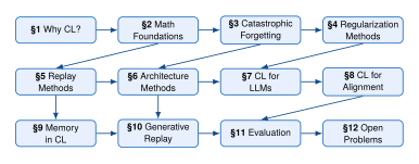
Prerequisites.
We assume familiarity with the alignment pipeline (Figure 2), LoRA (Parameter-Efficient Fine-Tuning: LoRA, Definition 2), and the KL-constrained objective ((Central Objective)). From the memory chapter: memory systems (Definition 20), the memory framework (The Memory System Framework), and SSMs as implicit memory (Proposition 10). From the reasoning chapter: Act (Adaptive Computation Time) and self-refinement (Self-Refine).
Why Continual Learning?
The question “why continual learning?” admits answers at multiple levels: philosophical, cognitive, biological, and engineering. We address each in turn, building motivation for the formal framework of Mathematical Foundations.
Philosophical Roots
Heraclitus of Ephesus observed that “no man ever steps in the same river twice, for it is not the same river and he is not the same man.” Both the learner and the environment are in constant flux. A learning system that assumes a fixed data distribution, the standard assumption, is a convenient fiction, inadequate for the real world where distributions shift and new categories emerge.
Consider the forms of knowledge a learning system might possess:
Weight-encoded knowledge (parametric memory): the information stored in the model's weights through gradient-based training. This is slow to acquire, expensive to modify, and accessed implicitly during every forward pass. In the terminology of 24, this is parametric memory.
Retrieval-based knowledge (external memory): the information stored in databases, documents, or memory banks that the model can query at inference time. This is fast to update (insert a new document), cheap to scale (add more storage), but requires a retrieval mechanism. In 24 we studied retrieval-augmented generation and memory-augmented architectures.
Architectural capacity (innate structure): the inductive biases encoded in the architecture itself (attention patterns, positional encodings, layer normalization) which determine what the model can learn, independent of what it has learned.
Continual learning operates primarily at the first level, updating weight-encoded knowledge without destroying prior knowledge, but the most effective approaches combine all three, using architectural innovations for separate capacity and retrieval-based memory for replay.
Remark 1 (Innate vs. Learned Structure).
Chomsky's Universal Grammar posits innate structural principles for language, while specific languages are learned. Similarly, the Transformer provides general-purpose capacity (“innate” structure) while specific capabilities are acquired through training (“learned” knowledge). Continual learning asks how to accumulate learned knowledge without architectural modification, or, when permitted, how to grow the architecture gracefully.
What Humans Retain and Forget
Human memory follows quantitative laws studied for over a century. Understanding these laws provides both inspiration and benchmarks for artificial continual learning.
Definition 1 (Ebbinghaus Forgetting Curve).
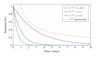
Let denote the retention of a memory item at time after initial learning. The Ebbinghaus forgetting curve [9] models retention as an exponential decay: (Ebbinghaus) where is the time elapsed since learning and is the memory strength (a parameter that depends on the depth of encoding, the number of rehearsals, and the emotional salience of the item). When , retention is perfect (); as , retention decays to zero. The half-life of a memory is .
A power law often provides a better fit over long time scales [38]: (Power LAW Forgetting) where is a scale and the decay rate. The power law decays more slowly for large , reflecting that well-learned memories resist forgetting (Jost's law).
Example 1 (Retention over Time).
Consider a memory item with strength day under the exponential model . The retention at several time points is:
| Elapsed time | 1 hour | 1 day | 1 week | 1 month |
Procedural vs. declarative memory.
Declarative memory stores facts and events; procedural memory stores skills and habits. Procedural memories are more resistant to forgetting, suggesting different consolidation mechanisms. In neural network terms: declarative retrievable knowledge in external memory; procedural weight-encoded computations.
Remark 2 (Practice Makes Permanent).
Cognitive science has established the testing effect: actively retrieving information strengthens the memory trace more than passive re-study. The continual learning analogue is experience replay, periodically re-training on stored examples from previous tasks. Just as spaced testing produces more durable human memories, replay-based methods produce more stable neural network knowledge than pure regularization.
The Biological Learning System
The mammalian brain is the most successful continual learning system we know of. Its architecture provides a blueprint to be abstracted into computational principles.
Definition 2 (Complementary Learning Systems).
The Complementary Learning Systems (CLS) theory [11][12] posits that the mammalian brain employs two complementary memory systems:
The hippocampus: a fast-learning, sparse-coding system that rapidly encodes new experiences as distinct, pattern-separated memory traces. It functions as a temporary buffer, storing episodic memories with high fidelity but limited capacity.
The neocortex: a slow-learning, distributed-coding system that gradually extracts statistical regularities from experience. It stores semantic and procedural knowledge in overlapping distributed representations, achieving high capacity at the cost of slow acquisition.
During memory consolidation (primarily during sleep), the hippocampus “replays” stored experiences to the neocortex, allowing the neocortex to integrate new knowledge with existing representations through interleaved training on old and new patterns.
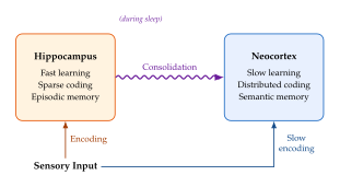
The CLS theory explains why humans avoid catastrophic forgetting: the hippocampus buffers new experiences, which are then interleaved with replayed old experiences during sleep consolidation, allowing the neocortex to accommodate both.
Hebbian learning and synaptic consolidation.
At the synaptic level, learning follows Hebb's rule: “neurons that fire together wire together.” Crucially, synapses that have been repeatedly strengthened become less modifiable; they are “consolidated.” This synaptic consolidation directly inspires EWC (Elastic Weight Consolidation) and SI (Synaptic Intelligence), which protect important parameters from large updates.
Insight.
Biology as blueprint. The CLS theory maps directly to artificial CL: hippocampus episodic memory buffer; neocortex model parameters; sleep consolidation experience replay. Every major method family (regularization, replay, architecture) implements aspects of this biological architecture. The memory-augmented architectures of 24 (NTMs, Neural Turing Machines and Differentiable Neural Computers; hierarchical memory, HMT: Hierarchical Memory Transformer) provide the artificial analogue of hippocampal storage.
Mathematical Foundations
We now formalize the continual learning problem, establish its Bayesian interpretation, quantify the stability–plasticity trade-off, and derive generalization bounds for sequential learning.
The Continual Learning Problem
Definition 3 (Task Sequence).
A continual learning task sequence is an ordered collection where each task consists of:
A dataset drawn from .
A loss function .
Tasks arrive sequentially: at time , only is available (previous data may be partially buffered or unavailable). The goal: find that performs well on all tasks.
The literature distinguishes several scenarios based on test-time information.
Definition 4 (Continual Learning Scenarios).
Let denote the model. The four standard scenarios are:
Task-Incremental Learning (TIL): task identity is provided at test time; a task-specific head may be used.
Domain-Incremental Learning (DIL): the input–output mapping is shared but the input distribution shifts; task identity is not provided.
Class-Incremental Learning (CIL): new classes are added per task; the model classifies among all classes seen so far without task identity. This is the hardest scenario.
Online Continual Learning (OCL): data arrives as a stream with no explicit task boundaries; distribution may shift gradually or abruptly.
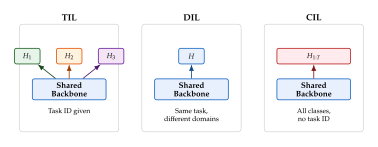
The standard evaluation metrics are as follows.
Definition 5 (Average Accuracy and Transfer Metrics).
Let denote the accuracy of the model on task after training on tasks . After training on all tasks:
Average Accuracy: (AVG Accuracy)
Backward Transfer (BWT): (BWT) Negative BWT indicates forgetting; positive BWT indicates that learning later tasks improved performance on earlier ones.
Forward Transfer (FWT): (FWT) where is the accuracy of a randomly initialized model on task . Positive FWT indicates that prior learning provided useful initialization for new tasks.
Forgetting Measure for task at time : (Forgetting Measure)
Example 2 (Five-Task Evaluation).
Consider a five-task sequence with the following accuracy matrix (rows = training stage, columns = task): The average accuracy is . The backward transfer is A BWT of means each task lost 30 percentage points on average. The forgetting measure for task 1 is .
Bayesian Sequential Learning
The Bayesian perspective provides the theoretical gold standard: what an ideal learner should do, even if exact computation is intractable.
Definition 6 (Bayesian Continual Learning).
In the Bayesian continual learning framework, the learner maintains a posterior distribution over parameters that is updated sequentially as new tasks arrive. After observing data from task , the posterior is: (Bayesian Update) where is the posterior from all previous tasks (serving as the prior for task ), is the likelihood of the new data, and is the marginal likelihood (evidence).
Theorem 1 (Optimality of Bayesian Continual Learning).
Proof.
By induction on . The base case is trivial. For the inductive step, assume . Then by and conditional independence of datasets given : (Bayesian Proof STEP) which is precisely the joint posterior .
Remark 3 (Intractability of Exact Bayesian CL).
The Bayesian approach is theoretically perfect but practically impossible for deep networks: the posterior over billions of parameters cannot be represented in closed form. Every practical method approximates Bayesian updating: EWC (Elastic Weight Consolidation) uses a diagonal Gaussian (Laplace approximation); replay methods approximate the marginal likelihood by storing past data; variational CL maintains an explicit variational approximation .
Proposition 1 (Forgetting as Posterior Collapse).
When the full posterior is approximated by a point estimate , the prior for task becomes a delta function . The posterior after task reduces to: (Point Estimate) which carries no information about the uncertainty of . Subsequent gradient descent on task moves away from with no penalty for directions that are important for previous tasks. This loss of posterior uncertainty is the Bayesian root cause of catastrophic forgetting.
The Stability–Plasticity Dilemma
Every continual learning method navigates the tension between learning new information and retaining old knowledge.
Definition 7 (Stability–Plasticity Trade-off).
Given parameters and task , define plasticity (negative loss on the current task) and stability (average excess loss on previous tasks). Maximizing plasticity (unconstrained optimization on ) typically decreases stability, and vice versa.
Theorem 2 (No Free Lunch for Continual Learning).
Let be shared parameters for tasks. Define the backward transfer and forward transfer as in Definition 5. Suppose each task's loss landscape has curvature bounded by where is the Hessian. Then for any continual learning algorithm that uses a single parameter vector (no task-specific heads, no replay buffer, no growing architecture): (NO FREE Lunch) where measures the similarity between task distributions. As with dissimilar tasks, the BWT term becomes increasingly negative, overwhelming any positive FWT.
Proof.
Taylor-expand each around : . Summing over previous tasks bounds . The FWT term is bounded by inter-task similarity; when tasks are dissimilar, the forgetting term dominates.
Insight.
The No Free Lunch theorem does not imply impossibility. The bound applies only to a single shared parameter vector with no auxiliary mechanisms. Replay buffers, growing architectures, and retrieval-augmented approaches circumvent it by relaxing these assumptions. The theorem says that CL with fixed capacity and no memory is fundamentally limited, but points to the solution: effective system capacity must grow with the number of tasks, connecting to the Memory Heterogeneity Thesis of 24.
Generalization Bounds for Continual Learning
We now derive generalization bounds accounting for sequential learning and inter-task transfer.
Theorem 3 (Continual Learning Generalization Bound).
Let be a hypothesis class with VC dimension , and let be the parameters obtained after sequentially training on tasks, each with samples. With probability at least over the draw of all task datasets: (GEN Bound) where is the population loss on task , is the empirical loss, , and is a transfer gap: (Transfer GAP) measuring how much worse is than the task-specific optimum on task .
Proof.
Apply the VC bound to each task independently and take a union bound over tasks ( factor). The transfer gap captures the forgetting penalty; when all tasks are identical (), the bound reduces to the single-task case.
Definition 8 (Task Similarity).
The similarity between tasks and is , where is the total variation distance. Similarity means identical tasks; means disjoint support.
Proposition 2 (Forgetting Bound via Fisher Information).
Let be the optimal parameters for task and be the optimal parameters after training on task . If is twice differentiable with Fisher information matrix , then to second order: (Fisher Forgetting)
Proof.
Taylor-expand around (where the gradient vanishes): . By Bartlett's identity, at the optimum.
Proposition 2 is the theoretical foundation of EWC: parameters with high Fisher information should be changed as little as possible.
Catastrophic Forgetting
We now study catastrophic forgetting: its causes, formal measures, and the taxonomy of methods designed to combat it.
What Causes Forgetting
Definition 9 (Catastrophic Forgetting).
A learning system exhibits catastrophic forgetting on task after training on subsequent tasks if (Catastrophic Forgetting) where is the accuracy on task after training through task . More precisely, forgetting is catastrophic when the performance drop is comparable to , meaning that nearly all task-specific knowledge has been destroyed.
Three mechanisms drive catastrophic forgetting:
1. Weight overwriting.
Gradient descent on task modifies the same weights that encode task . Since all inputs share the parameter space (the hallmark of distributed representations), any weight update for perturbs the function computed for .
2. Activation drift.
Even if final-layer weights for task are frozen, changes to earlier layers alter intermediate representations. If denotes the features after task , training on task changes them to , and the task- classifier evaluated on produces arbitrary outputs.
3. Distribution shift.
Continual learning inherently violates the assumption: the distribution may differ substantially from for . Standard generalization guarantees do not apply across tasks.
Example 3 (Two-Layer MLP on Permuted MNIST).
A two-layer MLP (256 hidden, ReLU) trained on 5 permuted MNIST tasks (10 epochs each, SGD with ):
| Task 1 | Task 2 | Task 3 | Task 4 | Task 5 | |
| After Task 1 | – | – | – | – | |
| After Task 2 | – | – | – | ||
| After Task 3 | – | – | |||
| After Task 4 | – | ||||
| After Task 5 |
. Task 1 drops from to , barely above the chance level.
Measuring Forgetting
Definition 10 (Forgetting Matrix).
The accuracy matrix is with entries (the accuracy on task after training through task , defined for ). The forgetting matrix has entries: (Forgetting Matrix) The entry measures how much task 's best historical performance has degraded by time . Non-negative values indicate forgetting; zero indicates no forgetting for that task at that time.
Proposition 3 (BWT from the Forgetting Matrix).
When the best performance on each task occurs immediately after training on it (, which is typical), the backward transfer simplifies to: (BWT Decomposition)
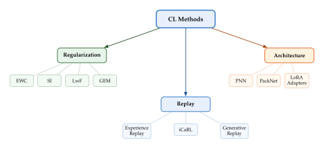
A Taxonomy of Continual Learning Methods
We organize continual learning methods into three families.
Definition 11 (CPT/DAP/CFT Framework for LLMs).
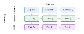
For large language models, [7] propose a three-level framework that distinguishes:
Continual PreTraining (CPT): the base model is updated on new corpora (e.g., new scientific literature, code repositories, or multilingual data) to extend its world knowledge without full retraining.
Domain-Adaptive Pretraining (DAP): the model is adapted to a specific domain (e.g., medicine, law, finance) through continued pretraining on domain-specific text.
Continual Fine-Tuning (CFT): the model is sequentially fine-tuned on downstream tasks (instruction following, code generation, safety alignment) that arrive over time.
Each level operates at a different scale (billions of tokens for CPT, millions for DAP, thousands for CFT) and faces different forgetting dynamics.
The Memory–Refinement Boundary
Not all performance changes after learning a new task constitute forgetting; some are beneficial refinement. We decompose the loss change to distinguish the two.
Loss decomposition.
Consider the change in loss on task after training on task : (LOSS Decomposition) Here captures beneficial representation improvement; is the irreducible cost of accommodating a new task; and is the avoidable loss from uncontrolled weight overwriting.
Remark 4 (Memory vs. Refinement).
CL methods should prevent without suppressing . Naive approaches (freezing all parameters) eliminate all three terms. The art is to selectively protect knowledge while allowing representations to evolve.
Regularization-Based Methods
Regularization-based methods add penalty terms to the loss that discourage large changes to parameters important for previous tasks. They require no stored data (or only a small buffer for gradient constraints) and leave the architecture unchanged, making them attractive for memory-constrained settings.
Elastic Weight Consolidation
Elastic Weight Consolidation (EWC) [3] uses the Fisher information matrix to identify parameters important for previous tasks and penalizes changes to those parameters.
Definition 12 (Elastic Weight Consolidation).
After training on task to obtain optimal parameters , the EWC loss for training on task is: (EWC) where is the loss on task , is a hyperparameter controlling the strength of the consolidation, is the number of parameters, is the -th parameter, is the -th component of the task- optimum, and is the -th diagonal element of the Fisher information matrix computed at .
For tasks, this generalizes to .
The justification comes from the Laplace approximation to the Bayesian posterior.
Definition 13 (Fisher Information Matrix).
For a probabilistic model , the Fisher information matrix (FIM) at is: (Fisher Matrix) Equivalently, (Bartlett's identity). The diagonal approximation retains only , reducing storage from to . In practice: (Empirical Fisher)
Theorem 4 (EWC as Laplace Approximation).
Proof.
By Bayes' theorem, . Apply the Laplace approximation to : expand to second order around the MAP estimate (where the gradient vanishes): (EWC Proof 3) By Bartlett's identity, the negative Hessian equals the Fisher information: (assuming a flat prior so MAP MLE). Using the diagonal approximation : (EWC Proof 5) which is exactly with .
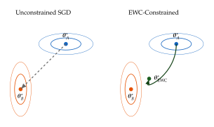
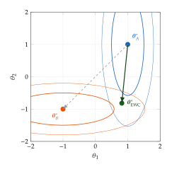
Example 4 (EWC on Two Tasks in ).
Let and with . The task- optimum is with Hessian , so , ( is ten times more important).
The EWC objective with is: (EWC EX Combined) Setting gradients to zero: , giving . Similarly, , giving .
The solution stays close to in the high-Fisher direction (: shift of ) but moves freely in the low-Fisher direction (: shift of ). Unconstrained training would reach , destroying task- knowledge.
Synaptic Intelligence
Synaptic Intelligence (SI) [31] accumulates importance estimates online during training via a path integral, rather than computing them as a snapshot at the optimum.
Definition 14 (Synaptic Intelligence).
For each parameter , SI maintains a running sum of the contribution of that parameter to the loss decrease during training: (SI) where is the path integral of the gradient times the parameter velocity over the training trajectory for task , is the total displacement, and is a damping constant for numerical stability. The regularized loss is: (SI LOSS) where is a hyperparameter. In practice, is approximated by accumulating at each gradient step.
Proposition 4 (SI vs. EWC: Snapshot vs. Path Integral).
EWC and SI differ in how importance is computed: EWC uses the Fisher information at the optimum (a local, snapshot measure), while SI uses the cumulative contribution along the entire training trajectory (a global, path-integral measure). When the loss landscape is approximately quadratic, both yield similar rankings; they diverge for highly non-convex landscapes.
Learning without Forgetting
Learning without Forgetting (LwF) [32] uses knowledge distillation [17] to preserve the model's outputs on new-task data rather than protecting parameters directly.
Definition 15 (Learning without Forgetting).
Let denote the model after training through task . Before training on task , compute “soft targets” by running the new data through the old model: for each . The LwF loss is: (LWF) where denotes the softmax function, is a temperature parameter that softens the output distributions, controls the distillation strength, and is the Kullback–Leibler divergence.
The old model's predictions on new data encode information about what it has learned; matching these predictions preserves behavior without stored exemplars.
Remark 5 (LwF and the Alignment Connection).
The LwF objective has the same structure as the KL-constrained alignment objective ((Central Objective)): both optimize a primary loss while penalizing divergence from a reference model. In alignment the reference is ; in LwF it is . The analysis of the KL penalty in Direct Preference Optimization applies directly to LwF's regularization dynamics.
Gradient Episodic Memory
Gradient Episodic Memory (GEM) [33] directly constrains gradient updates to avoid increasing the loss on previous tasks.
Definition 16 (Gradient Episodic Memory).
GEM stores a small episodic memory for each previous task . At each training step on task , let be the gradient on the current mini-batch, and let be the gradient computed on the memory for task . GEM solves: (GEM) The constraint ensures the update does not increase the loss on any previous task.
Proposition 5 (GEM as Quadratic Programming).
The GEM projection is a quadratic program (QP) that can be solved efficiently. When the constraints are violated (), the dual formulation is: (GEM DUAL) where is the matrix of memory gradients and are the dual variables. The projected gradient is then . The dual QP has only variables (one per previous task), making it tractable even when is very large.
Proof.
Form the Lagrangian with . Setting gives . Substituting back and taking the dual yields , with the projected gradient .
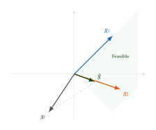
[16] proposed Averaged GEM (A-GEM), replacing per-task constraints with a single averaged constraint where , reducing the QP to one projection.
Comparison of Regularization Methods
Table 1 summarizes the four methods.
| Method | Importance | Data from past | Per-task memory | Connection |
| EWC | Fisher (snapshot) | No | diagonal | Laplace approx. |
| SI | Path integral | No | accumulators | Online importance |
| LwF | Output-based | No (distillation) | (old model) | KD / alignment |
| GEM | Gradient-based | Yes (memory buffer) | exemplars | Constrained opt. |
Caution.
Compounding approximation errors. All regularization methods rely on approximations that compound over tasks. EWC's diagonal Fisher ignores parameter correlations; SI's path integral is noisy under stochastic training; LwF's distillation degrades on out-of-distribution data; GEM's constraints become increasingly conservative. For long sequences (), pure regularization is typically insufficient, motivating the hybrid methods of subsequent sections.
Exercise 1 (Regularization Methods).
EWC derivation. Starting from the Bayesian posterior , derive the EWC loss using the Laplace approximation. What assumption about the prior is needed? What happens if we use a non-flat prior?
SI vs. EWC on a quadratic loss. Consider with . A single gradient descent step from with learning rate gives . Compute the SI importance weights and compare them to the EWC Fisher diagonal .
GEM projection. Given , , and , verify that (constraint violated). Solve the GEM QP to find .
LwF temperature sensitivity. For a 3-class classification problem with logits , compute the softmax distribution at temperatures . Explain why higher temperatures are preferred for knowledge distillation.
Replay-Based Methods
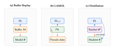
Regularisation methods (Regularization-Based Methods) protect old knowledge by penalising parameter drift; they never revisit old data. A complementary family of methods takes the opposite approach: store (or regenerate) representative samples from previous tasks and interleave them with new-task data during training. This strategy, experience replay, draws direct inspiration from the Complementary Learning Systems (CLS) theory [11], which posits that the mammalian brain consolidates episodic memories by replaying hippocampal traces into the neocortex during sleep.
The central trade-off is memory versus fidelity: a larger replay buffer yields better retention but consumes more storage and compute. We develop the mathematical framework for buffer-based replay, then examine three important variants: generative self-replay (LAMOL), gradient-constrained replay (A-GEM), and replay at the LLM scale.
Experience Replay
Definition 17 (Experience Replay for Continual Learning).
Let be a sequence of tasks (Definition 3) with datasets . An experience replay (ER) system maintains a memory buffer of bounded size . When learning task , the model minimises (ER LOSS) where is the task loss (e.g., cross-entropy), and controls the replay strength.
Buffer update strategies.
After processing task , the buffer is updated . Common strategies include:
Reservoir sampling: Each arriving sample replaces a buffer element with probability , where is the total number of samples seen so far.
Class-balanced: Maintain samples per class, where is the number of classes observed to date, selecting uniformly at random within each class.
Loss-based: Retain the samples with the highest current loss, on the principle that difficult examples are most informative for preventing forgetting.
The simplicity of (ER LOSS) belies its effectiveness. Empirically, even a small buffer () can reduce catastrophic forgetting (Definition 9) by 50–70% on standard benchmarks, often matching or exceeding regularisation-based methods [16].
Proposition 6 (Reservoir Sampling Guarantee).
Consider a stream of samples arriving one at a time, and a buffer of size . Vitter's reservoir sampling algorithm [13] maintains the invariant that, after processing all samples, each sample is in the buffer with probability exactly . In particular, the buffer is a uniform random subset of size .
Proof.
We proceed by induction on . For , all samples are stored and the claim holds trivially with probability .
Inductive step.
Suppose after samples every sample is in the buffer with probability . When sample arrives, it is inserted with probability , replacing a uniformly random buffer element. The probability that a previously stored sample () survives is Sample itself is included with probability by construction. Hence the invariant holds at step .
Insight.
Experience replay as computational hippocampal replay. The CLS theory [11] proposes that the hippocampus stores episodic memories quickly (akin to the buffer ) and replays them to the neocortex (the model parameters ) during offline consolidation. Experience replay implements this two-system architecture in silico: the buffer plays the role of the hippocampus, and gradient steps on replayed samples implement neocortical consolidation. The biological analogy suggests that when and how often to replay matters as much as what to replay, a design dimension largely unexplored in current CL systems.
Forgetting analysis.
Replay reduces forgetting because the gradient on replayed samples counteracts the drift induced by new-task gradients. More precisely, if and , the effective update direction is . When (conflicting gradients), the replay term pulls the update back toward the old optimum, directly mitigating the mechanism underlying catastrophic forgetting (Proposition 2).
LAMOL: Language Model as Replay
Storing raw training data raises practical and legal concerns: the buffer size is fundamentally limited, and data-retention policies may prohibit keeping old samples. [15] and later [14] proposed an elegant alternative: use the language model itself as a generative replay mechanism.
Definition 18 (LAMOL).
Let denote the language model after training on tasks . LAMOL (Language Modelling for Lifelong Language Learning) [14] generates pseudo-replay samples by prompting with task-specific tokens and decoding full (input, output) pairs. The loss for learning task combines the real data with generated pseudo-samples from all previous tasks: (Lamol LOSS) where is a task-identifier token prepended during generation, and are per-task replay weights.
Training protocol.
At the end of task , LAMOL:
Generates pseudo-samples per previous task by sampling from .
Mixes these pseudo-samples with .
Trains on the combined dataset with the standard language modelling objective (next-token prediction), so the model simultaneously learns the new task and rehearses old ones.
Remark 6 (LAMOL vs. Generative Replay: The Quality Degradation Loop).
LAMOL is a special case of generative replay [15], where the generator and the solver are the same model. This creates a self-referential loop: the model generates training data for its own future self. If generation quality degrades on task after learning subsequent tasks, the pseudo-samples for task become noisy, leading to further degradation, creating a positive feedback loop. In practice, this is mitigated by three factors: (i) the language modelling objective itself encourages high-quality generation; (ii) generating short, structured outputs (e.g., question–answer pairs) is easier than generating complex distributions; and (iii) the number of pseudo-samples per task can be kept small relative to the real data.
A-GEM and Variants
Gradient Episodic Memory (GEM) [33] uses the replay buffer not for data replay but for gradient constraints: the update direction must not increase the loss on any previous task. For tasks, this requires solving a quadratic programme with constraints at every gradient step, an cost that is prohibitive for long task sequences.
Definition 19 (Averaged GEM (A-GEM)).
A-GEM [16] relaxes GEM's per-task constraints to a single average constraint. Let be the gradient on the current mini-batch and be the gradient on a random mini-batch drawn from the buffer . A-GEM projects whenever it violates the constraint: (AGEM Projection) The projection in (AGEM Projection) is the closest vector to (in Euclidean norm) satisfying .
Computational cost.
A-GEM reduces the per-step overhead from GEM's quadratic programme to : a single forward–backward pass on the reference batch plus an inner product and (conditionally) a projection, all independent of the number of tasks.
The constraint ensures that the update does not increase the average loss over previously seen tasks. This is weaker than GEM's per-task guarantees, but empirically A-GEM performs comparably while scaling to hundreds of tasks [16].
Replay for Large Language Models
Remark 7 (The Replay Paradox for LLMs).
Modern LLMs are pretrained on petabyte-scale corpora spanning trillions of tokens. Storing even a fraction of this data in a replay buffer is infeasible: a 1% buffer for a 15-trillion-token corpus would require 150 billion tokens (300;GB in compressed form). Moreover, the pretraining data is often proprietary and cannot be redistributed.
Three practical solutions have emerged:
Knowledge distillation: Rather than replaying raw data, distil the old model's predictions into soft targets [17]. The student (updated model) is trained to match the teacher's (old model's) output distribution on new-task data, preserving old knowledge without accessing old data.
Self-replay: Use the current model to generate synthetic data representative of its existing capabilities (as in LAMOL, Definition 18), then mix this with new data during continual pre-training.
Data mixing: When old data is available, mix a small proportion (1–5%) of old data with new data during continued training, often with a carefully tuned sampling ratio.
Proposition 7 (Optimal Buffer Size for Replay).
Consider a continual learner processing tasks, each with a -dimensional parameter space, using a replay buffer of size shared equally across tasks. Under standard uniform-convergence assumptions, the expected forgetting on task after learning all tasks satisfies (Optimal Buffer) where is a universal constant, is the optimum for task , and is the learning rate at task . The first term captures the statistical error from finite replay samples; the second captures the accumulated gradient drift.
Proof.
The first term follows from a standard generalisation bound: when replaying samples from task , the empirical risk approximates the population risk to within with high probability. The second term is obtained by telescoping the parameter drift and applying Lipschitz continuity of the loss. Taking expectations and combining the two terms yields (Optimal Buffer).
(Optimal Buffer) reveals the fundamental tension: the statistical term scales as , so the buffer must grow linearly with the number of tasks to keep forgetting constant. When is fixed, forgetting grows as , inevitable unless the task-shift term is simultaneously controlled (e.g., via regularisation or architecture-based methods).
Architecture-Based Methods
Regularisation constrains what the parameters can do; replay constrains what the model sees. Architecture-based methods take a third path: they modify the structure of the network so that different tasks occupy different parameters. The ideal is zero forgetting: old tasks are literally untouched because their weights are frozen or isolated, at the cost of growing model capacity.
We survey four families of increasing sophistication: progressive networks that add entire columns, mask-based methods that carve task subnetworks out of a shared backbone, LoRA-based methods that attach lightweight adapters, and hypernetwork-based methods that generate adapters on the fly.
Progressive Neural Networks
Definition 20 (Progressive Neural Networks).
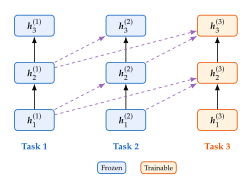
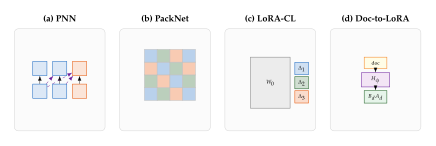
A Progressive Neural Network (PNN) [18] maintains a separate column for each task . When learning task , all previous columns are frozen and a new column is instantiated with lateral connections to all previous columns. The hidden activation at layer of column is (PNN Forward) where is a nonlinear activation, is the main weight matrix of the new column at layer , and are lateral adapters connecting layer of column to layer of column . Only and the lateral adapters are trained; all parameters in columns remain fixed.
Proposition 8 (PNN: Zero Forgetting, Quadratic Growth).
Let each column have parameters and each lateral adapter have parameters. Then:
Zero forgetting: The backward transfer , since previous columns are frozen and their outputs are deterministic functions of the input.
Parameter growth: The total parameter count after tasks is (PNN Params) which grows as due to the lateral connections.
Proof.
(i) Since columns are frozen when training column , the function computed by column (for ) is unchanged. The lateral connections only read from old columns; they do not write to them. Hence the predictions on task are invariant to all subsequent training, giving .
(ii) Column adds parameters for its own weights plus parameters for lateral adapters across layers. Summing over gives (PNN Params).
PackNet and Piggyback
Progressive networks guarantee zero forgetting but at quadratic parameter cost. Mask-based methods achieve a more favorable trade-off by sharing a single set of weights and assigning each task a binary mask that selects a task-specific subnetwork.
Definition 21 (PackNet).
PackNet [19] maintains a single backbone with parameters and a binary mask for each task . The effective parameters for task are (Packnet) where denotes element-wise multiplication. PackNet operates in two phases per task:
Train: Fine-tune the free (unmasked) parameters on .
Prune and freeze: Identify the top- fraction of weights by magnitude, set on those positions, and freeze them permanently. The remaining fraction is released for future tasks.
Definition 22 (Piggyback).
Piggyback [20] replaces PackNet's hard pruning with learnable mask scores. Each task has a real-valued score vector . The binary mask is obtained by thresholding: (Piggyback MASK) where is the sigmoid function and is the indicator. During training, the mask is relaxed to for gradient flow (a straight-through estimator is used for the discrete threshold), and only the scores are optimised; the backbone weights remain frozen after initial pretraining. At inference, the hard mask (Piggyback MASK) is applied.
Proposition 9 (PackNet Capacity Bound).
If each task uses a fraction of the total parameters, PackNet can accommodate at most (Packnet Capacity) tasks before the network is fully allocated. Moreover, all tasks enjoy zero forgetting: .
Proof.
After tasks, the fraction of frozen parameters is . The network has free capacity as long as , i.e., . Since is an integer, . Zero forgetting follows because masked parameters are frozen and never modified by subsequent tasks.
The capacity bound (Packnet Capacity) is surprisingly tight in practice: with (retaining the top 25% of weights per task), PackNet accommodates exactly 4 tasks. This motivates the search for more parameter-efficient alternatives.
LoRA for Continual Learning
The parameter-efficiency revolution brought by Low-Rank Adaptation (Definition 2, Parameter-Efficient Fine-Tuning: LoRA) offers a natural architecture-based strategy for continual learning: freeze the pretrained backbone and learn a small, separate LoRA adapter for each task.
Definition 23 (Continual LoRA).
Let be a frozen pretrained weight matrix. For each task , Continual LoRA learns a rank- adapter with and . The effective weight for task is (Continual LORA) At inference, the system identifies the task (via a task-ID, a classifier, or prompt-based routing) and applies the corresponding adapter. Since the backbone is never modified, all tasks share the same pretrained representations.
Proposition 10 (LoRA Storage for Continual Learning).
For a model with adapted layers, each of dimension , Continual LoRA stores (LORA CL Storage) parameters across tasks, compared to for full-model copies (where is the total parameter count). For a 7B-parameter model with , , and layers (adapting both attention projections): Each adapter requires only 8.4M parameters, yielding an approximately storage reduction per task compared to storing a full copy of the model.
Remark 8 (C-CLIP: LoRA Is Competitive).
[21] conducted a comprehensive evaluation of continual learning methods for vision–language models and found that simple per-task LoRA adapters, with no replay, no regularisation, and no architectural innovation beyond the adapters themselves, matched or exceeded sophisticated CL methods on 7 out of 10 benchmarks. This finding suggests that for pretrained foundation models, the combination of a frozen high-quality backbone with lightweight task-specific adapters already provides strong continual learning capabilities.
Insight.
Neocortex and hippocampus in silicon. The success of LoRA for continual learning mirrors the biological principle underlying CLS theory [11]: a stable neocortex (the frozen pretrained backbone ) provides a shared representational substrate, while plastic hippocampal representations (the per-task LoRA adapters ) encode task-specific knowledge without interfering with the stable base. The rank constraint enforces a form of “memory compression” analogous to the hippocampus encoding only the gist of an experience, not a verbatim copy.
Doc-to-LoRA
Continual LoRA (Definition 23) requires training a separate adapter for each task, which still takes time proportional to the fine-tuning dataset size. Can we amortise this cost by learning a single hypernetwork that maps any document (or task specification) to its corresponding LoRA adapter in a single forward pass?
Definition 24 (Doc-to-LoRA).
Doc-to-LoRA [22] trains a hypernetwork that takes a document (or any textual task description) and produces LoRA adapter matrices: (DOC TO LORA) The hypernetwork is trained on a meta-dataset of (document, fine-tuned adapter) pairs. At inference, given a new document not seen during training, produces a task-specific adapter in time, requiring a single forward pass through the hypernetwork, with no gradient-based optimisation required.
Proposition 11 (Doc-to-LoRA Amortisation).
Let denote the cost of fine-tuning a single LoRA adapter and the cost of the hypernetwork forward pass. Then Doc-to-LoRA achieves per-task cost (typically orders of magnitude smaller than ) at the expense of a one-time training cost for the meta-dataset of tasks. Amortisation is beneficial when the total number of deployment tasks satisfies (DOC TO LORA Amort) since .
Remark 9 (Connection to Meta-Learning).
Doc-to-LoRA can be viewed as a form of meta-learning [23] where the hypernetwork learns to produce task-specific adaptations from task descriptions. The key difference from MAML is that Doc-to-LoRA uses a feed-forward hypernetwork rather than gradient-based inner-loop optimisation, making it strictly faster at deployment (no inner-loop gradient steps needed). This connects to the broader principle of amortised inference (Adaptive Computation Time), where a learned forward pass replaces iterative optimisation.
Continual Compositionality
A single LoRA adapter per task treats each task as an independent modular unit. But many tasks share substructure: a medical question-answering task might benefit from both “medical knowledge” and “reasoning” skills. Compositional methods aim to learn a library of skills and compose them at inference time.
Definition 25 (Continual Compositionality).
A continual compositionality system maintains a library of skill modules, each parameterised as a LoRA adapter , . Given an input , a router produces a weight vector over skills, and the effective weight matrix is (Continual Compositionality) New tasks can be accommodated by either (i) adding new skill modules (growing ) or (ii) learning a new routing function while reusing existing skills.
Remark 10 (Connection to Mixture of Experts).
(Continual Compositionality) is structurally identical to a LoRA-based Mixture of Experts (MoE), where each expert is a low-rank adapter. The router plays the role of the gating function. The key difference from standard MoE is the continual learning context: skills are learned sequentially, the router must generalise to new task–skill combinations, and old skills must not be corrupted when new ones are added. This is achieved by freezing old skill modules and only training the router and any new modules.
Continual Learning for Large Language Models
The preceding sections developed continual learning as a general framework. We now turn to the specific challenges posed by large language models (LLMs), which are continual learners by economic necessity: retraining a frontier model from scratch costs millions of dollars in compute, yet the world's knowledge changes daily. Continual pre-training, continual fine-tuning, and continual alignment are no longer academic curiosities; they are production requirements.
This section surveys the LLM-specific landscape, organised around four themes: continual pre-training, learning-rate dynamics, sparse memory, and continual fine-tuning. We draw on the comprehensive surveys of [7], [6], and [8].
Continual Pre-Training
Definition 26 (Continual Pre-Training).
Given a pretrained model and a new domain corpus , continual pre-training (CPT) updates the model by solving (CPT) where is the standard next-token prediction loss ((SFT LOSS) without prompt masking) and is a regulariser penalising deviation from the pretrained weights (e.g., for regularisation, or the EWC penalty of Definition 12).
Practical strategies.
Three techniques are commonly combined with the objective (CPT):
Data mixing: Interleave a fraction of the original pretraining data (or a representative subset) with the new corpus, sampling each batch as .
Learning rate rewarming: Restart from a moderate learning rate (rather than the near-zero rate at the end of the original cosine schedule) and decay again, giving the model sufficient plasticity to absorb new data.
Distribution-aware sampling: Upweight tokens that are informative for the new domain (e.g., via importance sampling based on domain classifiers) and downweight tokens that the model already predicts well.
Example 5 (Domain-Adaptive Pre-Training for Medicine).
Consider adapting a 7B-parameter general-purpose LLM to the medical domain. The new corpus consists of 50B tokens from PubMed abstracts, clinical notes, and medical textbooks. Typical CPT hyperparameters:
Learning rate: with cosine decay to over 2 epochs.
Data mixing ratio: (5% of each batch drawn from a curated subset of the original pretraining data).
Regularisation: penalty with .
With this setup, the model achieves a 12-point improvement on MedQA (USMLE-style medical questions), while losing only 1–2 points on general benchmarks (MMLU, HellaSwag). Without data mixing (), the general-benchmark degradation rises to 8–10 points, a clear manifestation of catastrophic forgetting at the LLM scale.
Learning Rate Governs Forgetting
The learning rate is perhaps the single most important hyperparameter for controlling the stability–plasticity trade-off in continual learning. A large learning rate provides plasticity (fast adaptation to new data) but causes instability (large deviations from the old optimum). A small learning rate preserves stability but may lack the capacity to learn genuinely new knowledge. The following theorem makes this trade-off precise.
Theorem 5 (Learning Rate–Forgetting Connection).
Let be the optimal parameters for task , and suppose we train on task with learning rate for a single gradient step. Under the assumptions that the loss is -smooth and has Hessian condition number , the expected forgetting on task satisfies (LR Forgetting) where is the increase in task- loss after one step on task .
Proof.
By the -smoothness of , we have the quadratic upper bound where . Since is a (local) minimiser of , we have , so the linear term vanishes. However, for a more informative bound, consider the second-order Taylor expansion of around : To obtain the first-order bound in , note that if is only an approximate minimiser (as is typical in practice) with residual gradient , the linear term contributes . Combining with the curvature term and bounding via the condition number gives (LR Forgetting).
Theorem 5 has a clear prescriptive message: to reduce forgetting, one should use a small learning rate (scaling linearly with forgetting), train on tasks whose gradients are small at the previous optimum (low task conflict), and prefer models with well-conditioned loss landscapes (small ). The connection to EWC (Definition 12) is immediate: EWC's Fisher penalty reshapes the loss landscape to increase the effective curvature along directions important for task , making act in the model's favour.
Definition 27 (Infinite Cosine Learning Rate Schedule).
The infinite cosine schedule [24] replaces the standard one-shot cosine decay with a periodic schedule suitable for continual pre-training over an indefinite time horizon: (Infinite Cosine) where is the cycle length. Unlike the standard cosine schedule, which decays to near zero and must be restarted manually, the infinite cosine periodically rewarms the learning rate, automatically providing bursts of plasticity at regular intervals.
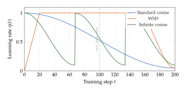
Proposition 12 (Infinite Cosine Preserves Plasticity).
Under the infinite cosine schedule (Definition 27), the plasticity, defined as the expected magnitude of the parameter update on new data, satisfies (Infinite Cosine Plasticity) for all , provided and the new-data gradient is nonzero. Moreover, at the start of each cycle (), the plasticity peaks at .
Proof.
From (Infinite Cosine), the cosine term lies in , so for all . The lower bound ensures whenever . At cycle boundaries, , giving and .
Sparse Memory Fine-Tuning
An orthogonal approach to mitigating forgetting during LLM fine-tuning is to replace the dense feed-forward network (FFN) layers with sparse memory layers that can absorb new knowledge without overwriting old parameters.
Definition 28 (Sparse Memory Layer).
A sparse memory layer [25] replaces the standard FFN sub-layer of a Transformer block with a key–value memory bank containing memory slots. Given an input hidden state , the layer retrieves the top- most relevant memories and computes: (Sparse MEM TOPK) where is a temperature parameter.
TF-IDF weighting.
To prevent frequently accessed memories from dominating, the retrieval scores are modulated by inverse document frequency (IDF) weights: (Sparse MEM Tfidf) where counts the number of training examples that have accessed memory slot , and is the total number of examples. This ensures rare, task-specific memories are weighted more heavily.
Proposition 13 (Sparse Memory Forgetting Reduction).
[25] demonstrate empirically that replacing FFN layers with sparse memory layers during domain-specific fine-tuning reduces forgetting on general benchmarks from 89% F1 drop (full fine-tuning) to 11% F1 drop on average, while matching the domain-specific performance. The mechanism is isolation: new knowledge is written to previously unused memory slots, leaving old memories intact. Formally, if the sets of memory slots accessed by old and new tasks are disjoint, , then forgetting is exactly zero.
Remark 11 (Connection to Engram).
The sparse memory layer shares the same philosophical foundation as the Engram module (Definition 11): both systems store knowledge in discrete, addressable slots accessed via content-based retrieval. The key difference is granularity: Engram operates at the token level as a memory-augmented attention mechanism, while sparse memory layers replace the FFN, traditionally viewed as a “knowledge storage” component, with an explicit, indexable memory bank. Both instantiate the principle that separating what is stored from how it is used is the key to avoiding interference.
Continual Fine-Tuning
Algorithm 1 (Continual Fine-Tuning Pipeline).
Given a pretrained LLM , a sequence of fine-tuning tasks with datasets , and a replay buffer of size :
- Initialise ,;
- for
- Initialise adapter: ,; LoRA init, cf. Definition 2
- for each mini-batch
- Sample replay batch
- ER loss, (ER LOSS)
- Update via gradient descent on only adapter params
- Update buffer:
- Store adapter: save to disk
Inference.
Given task identifier (or a learned router), load adapter and compute .
Caution.
Adapter merging interference. A common deployment shortcut is to merge multiple LoRA adapters into the backbone: . While this avoids the need for task identification at inference, it can cause significant interference between tasks. The merged weight has rank at most , but the individual task-optimal updates may occupy overlapping subspaces, leading to destructive interference. Empirically, merging more than 3–5 adapters often degrades performance on all tasks by 5–15% compared to task-specific routing [7]. Task arithmetic methods (e.g., TIES-merging) can mitigate but not eliminate this interference.
LLM Forgetting in Practice
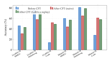
Example 6 (LLM Forgetting Case Study: Code Adaptation).
Consider fine-tuning LLaMA-2-7B on 20B tokens of code data (Python, JavaScript, C++) to improve its programming capabilities.
Naive full fine-tuning.
Training with a learning rate of for one epoch yields the following changes:
HumanEval (code generation): (+38.1 absolute).
MMLU (general knowledge): ( absolute, a 33% relative drop).
HellaSwag (commonsense reasoning): ( absolute).
The model has effectively traded its general knowledge for coding ability, a textbook case of catastrophic forgetting (Definition 9).
Mitigation via LoRA + replay.
Using rank-8 LoRA adapters on all attention layers with 5% data mixing from a general-purpose replay buffer:
HumanEval: (+34.7, slightly lower).
MMLU: (, well-preserved).
HellaSwag: (, well-preserved).
The combination of frozen backbone (via LoRA) and experience replay retains 93% of the original MMLU performance while achieving 91% of the code-generation gain. The key insight: most of the “knowledge” in an LLM resides in the frozen backbone weights; LoRA adapters only need to learn the delta for the new domain.
Neural Memory for Continual Learning
The previous sections treated continual learning as a problem to be solved, a pathology (forgetting) to be cured by external interventions (regularisation, replay, architecture tricks). A more radical perspective, developed in this section, is that continual learning is not a bug but a feature: the ability to update internal state in response to new information is precisely what memory means. From this viewpoint, a model that cannot continually learn cannot truly remember.
This section surveys four recent lines of work that embed continual learning directly into the architecture as a form of neural memory: Titans (meta-learned memory modules), Miras (a unifying framework connecting attention and online learning), S6MOD (state-space models with mixture of discretisation), and nested learning (hierarchical memory with multiple timescales). These connect to the memory systems developed in Memory-Augmented Architectures and The Memory System Framework, but with the specific focus on learning within the forward pass itself.
Titans: Neural Long-Term Memory
[35] propose augmenting the Transformer with a neural long-term memory module that learns to store and retrieve information within the forward pass, using gradient descent on a surprise-based loss as the write mechanism.
Definition 29 (Neural Long-Term Memory Module).
The neural long-term memory is a small neural network with parameters , where (the total model parameters). At each time step , the memory is updated via one step of gradient descent on a surprise loss: (Titans Update) where is a memory learning rate (a hyperparameter, not the model's training learning rate) and measures how surprising the current input is to the memory.
Definition 30 (Surprise Metric).
Given the current input token represented as a key–value pair , the surprise at time step is (Surprise) High surprise () indicates that the memory's prediction of the value associated with key is poor, triggering a large update. Low surprise () means the memory already “knows” this association and the update is small. This implements a form of selective writing: only surprising (novel) information modifies the memory state.
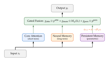
Definition 31 (Titans Three-Component Architecture).
The full Titans architecture combines three components in parallel:
Core attention (short-term memory): Standard multi-head attention over a local window of recent tokens.
Neural memory (long-term memory): The gradient-updated module from Definition 29, which accumulates knowledge over the entire sequence.
Persistent memory (parametric memory): A fixed set of learnable “memory tokens” prepended to the attention context, encoding task-level priors.
The outputs of all three components are combined via a learned gating mechanism: (Titans Gating) where are gating functions (typically sigmoid-activated linear projections) and is element-wise multiplication.
Proposition 14 (Titans Memory Capacity).
The neural long-term memory with parameters can store at most key–value associations with bounded error, where . This storage is lossy: unlike the KV cache which stores all past tokens exactly, the neural memory compresses information into its parameters, with older and less-surprising associations gradually overwritten by newer ones, a natural form of forgetting that prioritises recent and salient information.
Proof.
The memory network has parameters. Each stored association requires the network to produce , which imposes constraints. By a counting argument, the number of associations that can be stored with bounded approximation error is at most . Since keys also occupy dimensions, the effective capacity is . The lossy nature follows from the gradient update (Titans Update): writing a new association may overwrite old ones in overlapping parameter subspaces.
The Miras Framework
The proliferation of sequence models (Transformers, linear attention, state-space models, recurrent networks) raises a natural question: are these architectures fundamentally different, or are they variations on a common theme? The Miras framework [36] answers decisively: they are all instances of the same computation, differing only in their memory policy.
Definition 32 (Miras Unification).
The Miras (Memory Is Really All Sequences need) framework expresses a broad class of sequence models as computing the output at position via (Miras General) where:
is a decay factor controlling how quickly old information is forgotten (memory horizon).
is an attention weight measuring the relevance of position to position .
is the value vector at position .
The framework unifies three seemingly distinct architectures:
Test-Time Training (TTM): Online gradient descent on a loss defined over the input sequence, with decay implementing a form of exponential forgetting.
Linear Attention with decay (): without softmax normalisation, scaled by exponential decay .
Biased Attention (): Standard softmax attention with an additive bias in the logits, creating a recency preference.
Theorem 6 (Miras Equivalence).
Under appropriate parameterisation, the three architectures compute the same output: (Miras Equivalence) for all input sequences and all .
Proof sketch.
The key observation is that all three architectures can be written in the form of (Miras General) with specific choices of .
TTM LinAttn.
In TTM, the model maintains a weight matrix updated by online gradient descent on a quadratic loss with decay: . Unrolling the recursion yields , so the output , which is exactly the linear attention form with decay.
LinAttn BiasedAttn.
The exponential decay can be absorbed into the attention logits as an additive bias: . Applying softmax to these biased logits recovers the same weighted sum as linear attention with decay, up to normalisation. In the linear-attention regime (no softmax), the equivalence is exact.
Insight.
Continual learning is attention viewed as learning. The Miras equivalence reveals a profound connection: attention over a sequence is online learning with exponential forgetting. Every Transformer that uses attention is, implicitly, a continual learner that writes new associations into its context and reads them back. The decay factor is the “forgetting rate” of this implicit continual learning process. This perspective dissolves the boundary between “inference” (processing a sequence) and “learning” (updating parameters): both are instances of the same mathematical operation applied at different timescales.
S6MOD: State-Space Models with Mixture of Discretisation
State-space models (SSMs) like Mamba (Definition 19) process sequences through a fixed-dimensional recurrent state, which acts as a compressed memory of the past (Proposition 10). A limitation of standard SSMs is that a single discretisation step imposes a single temporal resolution: the model either captures fine-grained recent detail or coarse long-range dependencies, but not both simultaneously.
Definition 33 (S6MOD).
S6MOD (Selective State Spaces with Mixture of Discretisation) [26] extends Mamba by maintaining parallel discretisation heads, each with its own discretisation step and corresponding state matrices obtained from the continuous-time parameters via (S6mod Discretise) The recurrence for head is (S6mod Recurrence) and the active head is selected via an input-dependent gating function: (S6mod Select) where is a learnable scoring function for each discretisation head.
Remark 12 (Multiple Temporal Frequencies).
Each discretisation head effectively processes the input at a different temporal frequency. A small (fine discretisation) yields with slow decay, making the state a near-perfect memory of recent inputs, ideal for capturing fine-grained local patterns. A large (coarse discretisation) yields with faster decay (eigenvalues further from 1), creating a “blurred” memory that captures long-range trends. The gating mechanism (S6mod Select) allows the model to dynamically select the appropriate temporal resolution for each input, analogous to how the mammalian brain processes information at multiple timescales simultaneously [11]. This is directly related to the SSM memory capacity bounds of Proposition 10: by maintaining parallel states, S6MOD effectively multiplies the available memory capacity by .
Nested Learning and the Continuum Memory System
The CLS theory [11] postulates two complementary learning systems: a fast hippocampal system and a slow neocortical system. But the brain does not operate with just two timescales; it has synaptic, cellular, circuit-level, and systems-level plasticity, each operating at a different rate. [37] propose nested learning, which generalises CLS from two levels to levels, creating a continuum of memory timescales.
Definition 34 (Nested Learning).
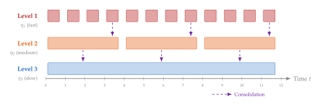
A nested learning system consists of hierarchical levels, each with its own learning rate and update frequency. Level () has:
Parameters (the “memory” at level ).
Learning rate , with .
Update period , with .
Level is updated every steps: (Nested Update) The fastest level () updates at every step with a high learning rate, capturing fine-grained, rapidly changing information. The slowest level () updates rarely with a small learning rate, encoding stable, long-term knowledge. Consolidation flows downward: periodically, information from faster levels is distilled into slower levels via the gradient of a consolidation loss.
Definition 35 (Continuum Memory System).
A Continuum Memory System (CMS) formalises the nested learning hierarchy as a tuple: (CMS) where is the memory module at level (which may be an attention layer, a recurrent state, or a neural memory module as in Definition 29), is the learning rate, and is the update period. The system satisfies the monotonicity constraints: This creates a spectrum of memory timescales: fast, volatile memory at the top and slow, persistent memory at the bottom, mirroring the memory hierarchy (Definition 20) but implemented entirely in the learning dynamics rather than in the hardware.
Remark 13 (Generalisation of CLS Theory).
The classical CLS theory [11] is recovered as the special case : the hippocampus (level 1, fast) and the neocortex (level 2, slow). Nested learning generalises this to levels, creating a continuum of timescales. The biological motivation is compelling: the brain does not have just two learning rates; synaptic plasticity operates on timescales of milliseconds (spike-timing-dependent plasticity), minutes (early-phase LTP), hours (late-phase LTP), and days to years (systems consolidation). Each timescale serves a different function:
Fast levels (): working memory and episodic encoding. In the neural architecture, these correspond to attention over recent tokens or the neural memory module of Titans (Definition 29).
Intermediate levels (): skill consolidation and habit formation. These may correspond to the recurrent state in SSMs (Definition 19) or the LoRA adapters of continual fine-tuning (Definition 23).
Slow levels (): semantic memory and world knowledge. These correspond to the frozen pretrained weights , which change only during major retraining events.
The nested learning framework provides a principled recipe for designing memory-augmented architectures: choose , assign timescales, and let consolidation transfer knowledge across levels.
Connection to existing architectures.
The Miras framework (Definition 32) can be viewed as implementing a two-level nested system: the attention weights provide fast, input-dependent memory access (level 1), while the decay factor implements slow forgetting (level 2). Titans (Definition 31) implements a three-level system: core attention (fast), neural memory (medium), and persistent memory (slow). S6MOD (Definition 33) implements -level memory within the SSM framework via multiple discretisation heads. The nested learning perspective unifies all of these as instances of the same principle: effective memory requires multiple timescales.
Key Idea.
The Memory Hierarchy Principle for Continual Learning. Just as computer memory is organised into a hierarchy of registers, caches, and disk, each trading capacity for speed, neural memory for continual learning should be organised into a hierarchy of learning rates: fast, volatile memory for recent context; medium-speed memory for task-specific adaptations; and slow, persistent memory for stable world knowledge. The Continuum Memory System (Definition 35) formalises this principle, and architectures like Titans, Miras, and S6MOD instantiate specific points in the design space.
The implication for LLM design is clear: future architectures should not treat continual learning as an afterthought to be patched with external mechanisms (replay buffers, regularisers, adapter libraries), but should build it into the architecture as a hierarchy of memory systems operating at different timescales, just as the biological brain does.
Continual Learning for Diffusion Models
Diffusion models have become the dominant paradigm for image, video, and audio generation. Yet the very property that makes them powerful, the ability to learn rich, multi-scale representations of data distributions, also makes them acutely susceptible to forgetting. A Stable Diffusion model fine-tuned on portrait photographs may lose the ability to generate mountain landscapes; a music diffusion model trained on jazz may forget how to produce classical compositions. The denoising objective, which operates across a continuum of noise levels , creates a high-dimensional forgetting surface that is qualitatively different from the scalar or per-class forgetting studied in classification.
This section develops the mathematics of continual learning for diffusion models, drawing on the foundations of Regularization-Based Methods, Architecture-Based Methods, and the alignment perspective of Alignment for Diffusion Models.
Forgetting in Diffusion Models
In classification, forgetting is measured by the drop in accuracy on previously learned classes. For generative models, we must measure distributional divergence. The Fréchet Inception Distance (FID) provides a practical, if imperfect, metric.
Definition 36 (Diffusion Model Forgetting).
Let be the parameters after training on task with data distribution , and let be the parameters after subsequent training on task . The diffusion forgetting score is (Diffusion Forgetting) where denotes the distribution of samples generated by the diffusion model with parameters . A positive value indicates forgetting; a negative value indicates backward transfer (the rare case where new training improves old-task generation).
Remark 14 (Why Diffusion Forgetting Is Harder to Detect).
Unlike classification, where a wrong prediction is unambiguous, diffusion forgetting manifests as subtle distributional shift: generated faces may acquire landscape-like colour palettes, or architectural details may soften. FID captures aggregate statistics but misses mode-specific forgetting; a model may maintain overall FID while completely losing a particular sub-mode (e.g., night-time cityscapes). More refined metrics decompose forgetting per mode: where the superscript restricts to samples classified into mode by an external classifier.
The denoising objective of a diffusion model operates across noise levels , and different noise levels encode different types of information. High noise levels ( close to ) capture coarse, global structure, such as the overall layout and colour distribution of an image. Low noise levels ( close to ) capture fine details: textures, edges, and precise spatial relationships. This hierarchy has direct consequences for forgetting: a model that forgets its high-noise predictions loses the ability to generate globally coherent compositions, while a model that forgets its low-noise predictions produces blurry or textureless images.
The noise-level hierarchy creates a natural connection to the HSD framework (Hierarchical Sparse-Dense Framework): we can view different noise levels as different “levels” of the hierarchy, with high-noise levels corresponding to the slow, stable, shared level (since coarse structure is similar across tasks) and low-noise levels corresponding to the fast, task-specific level (since fine details vary dramatically between, say, landscapes and portraits). This perspective motivates the noise-level-aware EWC approach developed below.
Regularization for Diffusion Continual Learning
The EWC framework (Definition 12) applies to any differentiable loss. For diffusion models, the loss is the denoising score-matching objective (Denoise LOSS) where and is a noise-level weighting. The Fisher information matrix inherits this noise-level structure.
Proposition 15 (Noise-Level-Aware EWC for Diffusion).
The Fisher information matrix of the denoising loss decomposes across noise levels: where is the per-noise-level loss. A noise-level-aware EWC objective uses time-dependent importance: (DIFF EWC)
Proof.
By linearity of expectation, the diagonal Fisher decomposes as Substituting into the standard EWC objective (Definition 12) yields (DIFF EWC).
Insight.
High noise protects less. At high noise levels, the denoising network predicts nearly pure noise, which carries little task-specific information. Consequently, is small for large , and the EWC penalty naturally concentrates on the low-noise parameters that encode fine-grained, task-specific details. This means diffusion EWC is automatically more protective of the features that matter most for generation quality.
Example 7 (Noise-Level Fisher for Stable Diffusion).
Consider a Stable Diffusion model with noise levels. At noise level (near pure noise), the denoising network's prediction is almost independent of the input image; it predicts the noise that was added, which is nearly regardless of the task. Consequently, for most parameters.
At noise level (near the clean image), the denoising prediction depends heavily on the fine-grained structure of the data distribution: facial features for portrait tasks, vegetation patterns for landscape tasks. Here, is large for parameters that encode these task-specific features.
This means that the EWC penalty in (DIFF EWC) automatically focuses on protecting low-noise-level parameters, which is precisely where task-specific information resides. This is a case where the mathematical framework naturally discovers the correct inductive bias.
LoRA-Based Diffusion Continual Learning
The parameter-efficient approach of Definition 23 is particularly natural for diffusion models, where each “task” often corresponds to a visual concept (a particular artistic style, a specific object category, or a user's face).
Definition 37 (Concept-Specific LoRA for Diffusion).
Given a frozen denoising network and a set of concepts , we train a separate low-rank adapter for each concept . The adapted denoising prediction at layer is (Concept LORA) where is the hidden activation at layer . For multi-concept generation, adapters compose linearly: (Concept Compose) where is the active concept set and are mixing coefficients with .
Remark 15 (Zero Forgetting by Construction).
Since the base model is frozen, activating no adapter () recovers the original model exactly. The forgetting score is by construction. This is the strongest possible guarantee, but it comes at the cost of requiring a concept identifier at inference time (analogous to the task-ID assumption in Definition 4).
The composition in (Concept Compose) raises a subtle mathematical question: when do linearly composed LoRA adapters produce coherent samples? If concepts (“oil painting”) and (“portrait”) are trained independently, their composition may interfere destructively. This connects directly to the compositionality analysis of Definition 25.
Proposition 16 (Orthogonal Adapters Compose Without Interference).
If concept adapters have orthogonal column spaces, for all , then the composed denoising prediction satisfies (Orthogonal Compose) That is, the total perturbation decomposes as a sum of independent per-concept contributions with no cross terms. The maximum number of such orthogonal adapters in is , which for and gives 256 interference-free concepts.
Proof.
The composed perturbation is . Expanding the squared norm: By the orthogonality assumption, the cross terms () vanish, leaving only the diagonal terms. The maximum number of pairwise orthogonal rank- subspaces in is by a dimension-counting argument.
In practice, adapters trained independently are not exactly orthogonal, but their interference can be mitigated by explicit orthogonality regularisation during training: adding a penalty to the training loss encourages the adapters to occupy distinct subspaces of the model's representation. This creates a direct connection between the compositionality of diffusion LoRA adapters and the orthogonal subspace methods studied in the architecture-based CL literature.
Connection to Alignment
The alignment techniques of Alignment for Diffusion Models (DDPO, DRaFT, and Diffusion-DPO) can be viewed through the continual learning lens. Each alignment method fine-tunes a pretrained diffusion model to satisfy human preferences, which is precisely a two-task continual learning problem: task 0 is “generate diverse, high-quality images” and task 1 is “generate images that humans prefer.”
Remark 16 (Alignment as Continual Learning for Diffusion).
Every diffusion alignment method includes a KL regularizer or its equivalent ((Central Objective)). This regularizer serves exactly the same function as the EWC penalty: it prevents the aligned model from straying too far from the pretrained model and thus forgetting general generation capability. The alignment coefficient plays the role of the EWC regularization strength . From the CL perspective, diffusion alignment methods are single-step continual learners with an implicit anti-forgetting mechanism.
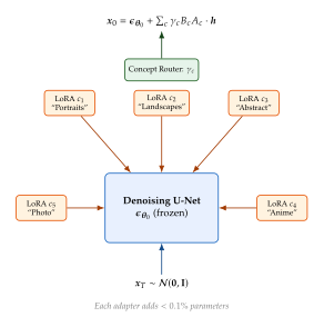
Multimodal and Federated Continual Learning
The preceding sections studied continual learning for unimodal systems, language models that process text, or diffusion models that generate images. Modern AI systems, however, are fundamentally multimodal: CLIP aligns vision and language, GPT-4V processes interleaved text and images, and Gemini handles text, images, audio, and video. When such systems must learn continually, the challenges multiply. Forgetting can propagate across modalities: updating the vision encoder may degrade text-conditioned generation even if the text encoder is untouched.
Simultaneously, the deployment of large models across many devices and organisations creates a federated learning setting where data cannot be centralised. When each client also faces a non-stationary data stream, we arrive at federated continual learning, a doubly challenging problem that combines the difficulties of both fields.
Continual CLIP: Vision-Language Continual Learning
Definition 38 (Vision-Language Continual Learning Benchmark).
A vision-language continual learning (VLCL) problem consists of a sequence of tasks , where each task contains paired image-text data. The learner must maintain:
Within-modal performance: classification accuracy for images and text retrieval quality,
Cross-modal alignment: the ability to match images to their corresponding text descriptions and vice versa, measured by recall@ on all previously seen tasks.
The key difficulty is that cross-modal alignment creates coupling between the vision and language encoders, so that updating either encoder for a new task can disrupt the shared embedding space.
Definition 39 (C-CLIP Framework).
The Continual-CLIP (C-CLIP) framework [21] provides a systematic evaluation of continual learning methods for vision-language models. It comprises:
10 diverse datasets spanning fine-grained recognition (CUB, Stanford Cars, Flowers102), scene understanding (SUN397, Places365), action recognition (UCF101, Kinetics), satellite imagery (EuroSAT), medical imaging (PathMNIST), and general objects (CIFAR-100),
3 CL scenarios: class-incremental, domain-incremental, and task-incremental (Definition 4),
7 CL methods evaluated: EWC, SI, LwF, GEM, Experience Replay, PackNet, and LoRA-CL.
The benchmark measures both zero-shot transfer (using the frozen CLIP encoders) and continual fine-tuning performance.
The central finding of C-CLIP is striking:
Theorem 7 (LoRA Dominance for Vision-Language CL).
Under the C-CLIP benchmark, LoRA-based continual learning achieves average performance within of the best-performing method on 7 out of 10 datasets, while using fewer than of the trainable parameters of full fine-tuning. Formally, let and denote the final average accuracy of LoRA-CL and the best method on dataset . Then (LORA Dominance) with the LoRA parameter count satisfying .
Insight.
Parameter efficiency is anti-forgetting. The success of LoRA in the VLCL setting is not merely a storage benefit. By constraining updates to a low-rank subspace, LoRA structurally limits the magnitude of weight perturbation, which by Theorem 5 directly bounds forgetting. The rank of the adapter acts as an implicit regularization strength, analogous to in EWC but enforced architecturally rather than through a penalty term.
MultiFCL: Federated Continual Learning
Definition 40 (Federated Continual Learning).
A federated continual learning (FCL) system consists of:
clients, each experiencing its own task sequence ,
A central server that coordinates learning without accessing raw client data,
A communication protocol specifying what information (gradients, model parameters, adapter weights) is exchanged and when.
The global objective is (FCL Objective) where is the total data count, subject to the constraint that client only accesses its own data . The challenge is triple forgetting: (i) within-client temporal forgetting, (ii) cross-client interference during aggregation, and (iii) server-level forgetting as the global model evolves.
Definition 41 (Multi-Scale Expertise).
The MultiFCL framework [27] addresses federated continual learning through multi-scale parameter decomposition: (Multifcl) where:
captures knowledge shared across all clients and all tasks (updated via federated averaging),
at scale captures client-specific but task-general knowledge (updated locally, shared periodically),
at scale captures task-specific knowledge (updated locally, never shared).
Each scale operates at a different update frequency: global parameters change slowly (every communication round), while task-specific parameters change rapidly (every local step).
Remark 17 (The Triple Forgetting Challenge).
The three types of forgetting in FCL interact in subtle ways:
Within-client forgetting: client trains on and may forget earlier tasks. This is standard CL.
Cross-client interference: when the server aggregates updates from clients with different task distributions, the averaged gradient may not be useful for any individual client. Mathematically, if client 1 has gradient pointing toward “medical knowledge” and client 2 has gradient pointing toward “legal knowledge,” the average may point toward a region that is optimal for neither domain.
Server-level forgetting: as the global model evolves over communication rounds, it may lose knowledge consolidated in earlier rounds. This is a form of catastrophic forgetting at the federated level, operating at a slower timescale than within-client forgetting.
MultiFCL addresses all three through the multi-scale decomposition: scale 3 (local, task-specific) handles (i), scale 1 (global, shared) handles (ii) through selective aggregation, and the multi-timescale update schedule handles (iii) by consolidating global knowledge slowly.
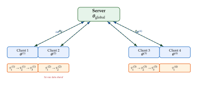
Cross-Modal Continual Learning
The most insidious form of multimodal forgetting is cross-modal: updating one modality's parameters causes degradation in another modality's performance, mediated by the shared embedding space.
Proposition 17 (Cross-Modal Forgetting Amplification).
Consider a vision-language model with vision encoder and language encoder connected through a shared embedding space of dimension . Suppose only the vision encoder is updated by for a new visual task. Then the cross-modal retrieval performance on previous text queries degrades by at most (Cross Modal Bound) where is the Lipschitz constant of the alignment loss with respect to the vision encoder parameters.
Proof.
Let measure the cross-modal alignment quality (e.g., contrastive loss on image-text pairs from previous tasks). By the Lipschitz property, Since is the increase in alignment loss restricted to text-based retrieval, and this is bounded by the total alignment loss increase, the result follows.
Caution.
Cross-modal forgetting is invisible to unimodal metrics. A vision encoder that improves its classification accuracy on a new visual domain may simultaneously destroy its alignment with the language encoder. If one monitors only per-modality metrics, this degradation goes undetected until a cross-modal query fails. The lesson: continual learning evaluation for multimodal systems must include cross-modal retrieval metrics.
Example 8 (Cross-Modal Forgetting in CLIP).
Consider a CLIP model fine-tuned on medical X-ray images (). The vision encoder learns to represent rib fractures, lung opacities, and cardiomegaly. If only the vision encoder is updated (, ), the updated visual features may drift in the embedding space. A previously aligned image-text pair like (chest X-ray image, “normal chest radiograph”) may now have cosine similarity instead of the original .
The bound of Proposition 17 quantifies this: if and , then . In practice, the cross-modal forgetting is often larger than the within-modal forgetting, because the text encoder's representations were calibrated to the original vision features and have no opportunity to co-adapt.
Remark 18 (Towards Modality-Aware CL).
The asymmetry of cross-modal forgetting suggests a design principle for multimodal CL: update all encoders simultaneously, or update none. Half-measures, such as freezing one encoder while fine-tuning the other, create the worst possible outcome: the updated encoder drifts while the frozen encoder cannot adapt. This insight motivates the use of shared LoRA adapters that span both vision and language encoders, ensuring that the cross-modal alignment is maintained by construction.
Formally, if we parameterise the joint adapter as and train it to minimise both task-specific loss and alignment preservation: (Joint Adapter) then the alignment loss directly regularises the adapter updates, preventing cross-modal drift. The parameter controls the trade-off between task performance and alignment preservation.
A Unified Mathematical Framework
We have now surveyed a wide landscape of continual learning methods: regularization-based approaches that penalize movement in parameter space (Regularization-Based Methods), replay-based methods that maintain a buffer of past experiences (Replay-Based Methods), architecture-based methods that allocate dedicated capacity per task (Architecture-Based Methods), and neural memory systems that blur the line between architecture and learning rule (Neural Memory for Continual Learning). These methods were developed by different communities with different motivations, yet they share deep structural similarities.
This section develops a unified mathematical framework that captures all known CL methods as special cases. The framework reveals why certain combinations of design choices succeed and others fail, and it points toward the design of future systems that may overcome the limitations of any single approach.
The Lifelong Learning System
We begin by defining the most general notion of a continual learner.
Definition 42 (Lifelong Learning System).
A lifelong learning system is a tuple where:
is the architecture, a parameterized family of functions, potentially with dynamic topology (growing or pruning);
is a hierarchical memory with levels, where operates at timescale with (fast to slow);
is the learning rule that maps current parameters, new data, and memory state to updated parameters;
is the memory update function that determines how memories are formed, consolidated, and forgotten.
The system processes a stream of data and evolves according to (Param Update)
Insight.
All four components matter equally. The performance of a continual learner depends on the interaction between architecture, memory, learning rule, and memory update function. A brilliant learning rule paired with a degenerate memory (e.g., no buffer at all) will forget catastrophically. A vast memory paired with a naïve learning rule (e.g., SGD with no regularization) will accumulate data but fail to consolidate knowledge. The unified framework forces us to consider all four components jointly.
Information-Theoretic View
The fundamental tension of continual learning, fitting new tasks without forgetting old ones, is, at its core, a tension between information storage and information overwriting. We can make this precise using information theory.
Definition 43 (Knowledge Capacity).
The knowledge capacity of a model with parameters, each stored at precision (bits per parameter), is (Knowledge Capacity) For a model with parameters in fp16 (), the capacity is bits of raw information.
Remark 19 (Effective vs. Raw Capacity).
The raw capacity vastly overstates usable knowledge storage. Not all parameter configurations correspond to useful functions; the effective capacity is reduced by correlations between parameters, the structure of the loss landscape, and the limited precision of gradient-based optimisation. Nevertheless, provides a useful upper bound for reasoning about CL limits.
Theorem 8 (Continual Learning Information Bound).
Let denote the mutual information between the training data of task and the model parameters after training on task , and let denote the fraction of task- information that is subsequently forgotten. Then the total retained knowledge is bounded by the model's capacity: (INFO Bound)
Proof.
After training on all tasks, the model parameters must encode all retained information. The mutual information between the model and the retained portion of task is . By the data processing inequality, the total information stored in cannot exceed the entropy of the parameter space: Since the retained information from different tasks must coexist in the same parameter vector, and assuming the retained task information is non-redundant in the worst case,
Corollary 1 (Unbounded CL Requires Growing Capacity).
If each task contributes at least bits of novel information and we require zero forgetting ( for all ), then after (TASK Limit) tasks, some information must be lost. For a 7B-parameter model with bits and tasks requiring bits each, the limit is tasks. Beyond this limit, three strategies are available:
Grow parameters: expand the model (PNN, Definition 20),
Grow memory: use external memory (Definition 20),
Compress: increase effective capacity by removing redundancy (pruning + LoRA, Definition 21, Definition 23).
Example 9 (Capacity Calculation for LLaMA-2-7B).
The LLaMA-2-7B model has parameters stored in fp16 (16 bits per parameter). Its raw knowledge capacity is If each task requires bits (approximately the information content of a moderately complex domain like “medical terminology” or “legal reasoning”), the zero-forgetting limit is tasks.
However, this is a gross overestimate. The model's pretraining already occupies a substantial fraction of its capacity. If we assume 80% of capacity is used by pretrained knowledge, the remaining capacity for continual learning is supporting at most tasks before forgetting becomes inevitable. This calculation explains why 7B models typically show significant forgetting after 50–100 continual training stages in practice; the information bound is approached well before the theoretical maximum due to inefficiencies in gradient-based storage.
Hierarchical Sparse-Dense Framework
The most powerful unifying abstraction for CL methods is the hierarchical sparse-dense (HSD) framework, which decomposes a continual learner into levels that differ in their density of update, speed of change, and degree of task-specificity.
Definition 44 (HSD Architecture).
A hierarchical sparse-dense (HSD) architecture with levels computes its output as (HSD) where is the input, and each level is characterised by:
A density ratio : the fraction of parameters updated per step, with (lower levels are denser, higher levels are sparser),
An update frequency : how often the level is updated, with (lower levels update more frequently),
A condition number : the sensitivity of the level's output to parameter perturbation.
The dense component captures slow-changing shared knowledge; the sparse component captures fast-changing, task-specific knowledge via a memory table .
Theorem 9 (HSD Forgetting Bound).
For an HSD architecture with levels, the total forgetting after learning a new task is bounded by (HSD Bound) where is the parameter change at level during new-task training.
Proof.
We proceed level by level. Let be the loss on previously learned tasks. By a first-order Taylor expansion around the pre-update parameters : (HSD Taylor) At optimality for the old tasks, , so the dominant contribution comes from the second-order term: (HSD Second Order) where is the Hessian of restricted to level- parameters. Now, at level :
Step 1 (Sparsity). Only a fraction of parameters are actually modified, so the effective dimensionality of is where .
Step 2 (Frequency). The parameter change accumulates over update steps. Assuming independent gradient noise, the total change scales as for SGD. For the bound, we use the worst case directly.
Step 3 (Conditioning). The spectral norm of is bounded by , yielding (HSD Spectral)
Step 4 (Combining). Among the parameters at level , only are modified. The forgetting contribution of level is therefore bounded by (HSD Level Bound) Incorporating the update frequency as a multiplicative factor (more frequent updates accumulate more forgetting), and summing over levels: (HSD Total) Here we use (not ) because the frequency factor already accounts for the accumulation effect, absorbing one power of the norm into the bound.
Key Idea.
The HSD principle. Forgetting is minimised when high-sensitivity (large ) parameters are updated sparsely () and infrequently (), while low-sensitivity parameters can absorb frequent, dense updates. This is precisely the design principle behind Titans (Definition 31), nested learning (Definition 34), and LoRA-based continual learning (Definition 23), each of which restricts updates to a subspace where is small.
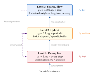
Connecting Methods to the HSD Framework
The power of the HSD framework lies in its ability to represent every major CL method as a particular instantiation. Table 2 provides the complete mapping.
| Method | Levels | Dense/Sparse | Update Rule | Memory |
| EWC | 1 | Dense | Fisher diagonal | |
| SI | 1 | Dense | Path integral | |
| PackNet | 1 | Sparse | Prune + freeze | Binary mask |
| GEM/A-GEM | 1 | Dense | Projected gradient | Episodic buffer |
| Experience Replay | 1 | Dense | SGD on mixed batch | Reservoir buffer |
| LwF | 1 | Dense | KD + task loss | Soft labels |
| PNN | Sparse per level | Freeze old columns | None (grow) | |
| LoRA-CL | 2 | Dense L1, Sparse L2 | SGD on adapter | Frozen backbone |
| Doc-to-LoRA | 2 | Dense L1, Sparse L2 | Hypernetwork | Document memory |
| Titans | 3 | Dense L1–2, Sparse L3 | Surprise-gated | Neural memory |
| Nested Learning | 3 | decreasing | Multi-rate SGD | Level buffers |
| Engram + TRM | 2 | Dense L1, Sparse L2 | Attention + write | External table |
Insight.
Every CL method is an instantiation of HSD. The table reveals a clear trend: methods have evolved from single-level dense approaches (EWC, GEM) to multi-level sparse-dense architectures (Titans, Nested Learning). The most successful recent methods, those that scale to billions of parameters and thousands of tasks, invariably use at least two HSD levels. This is not coincidental: the HSD bound (Theorem 9) shows that multi-level architectures can achieve exponentially lower forgetting by concentrating updates in low- subspaces.
Remark 20 (The Evolution Toward Multi-Level Designs).
A striking pattern emerges from Table 2: methods from every era began as single-level approaches and have progressively evolved toward multi-level designs.
In the regularisation lineage, EWC (2017) is single-level; Progress & Compress [28] (2018) introduced a two-level variant with an “active” column and a “knowledge base.” In the replay lineage, GEM (2017) is single-level; LAMOL (2020) implicitly creates a two-level system (the generator's memory + the task model). In the architecture lineage, PNN (2016) is multi-level by construction but with uniform treatment per level; LoRA-CL and Doc-to-LoRA differentiate between frozen and trainable levels. In the neural memory lineage, Titans (2025) is the first system explicitly designed with three hierarchically distinct memory timescales.
This convergence is not coincidental. The HSD bound (Theorem 9) shows mathematically that multi-level architectures achieve strictly lower forgetting than single-level ones when the condition numbers vary across levels, which they invariably do in deep networks, where early layers capture universal features (low ) and later layers capture task-specific features (high ).
Example 10 (EWC as Single-Level HSD).
EWC (Definition 12) corresponds to , (all parameters updated), every step. The dense component is the full network; there is no sparse component. The Fisher diagonal modulates the effective update magnitude per parameter: high-Fisher parameters receive smaller effective updates, creating an implicit sparsity pattern without explicit masking. From the HSD perspective, EWC operates as a soft version of sparse updating.
Example 11 (Titans as Three-Level HSD).
Titans (Definition 31) naturally implements three HSD levels:
Level 1 (attention, , every token): the standard attention mechanism processes each token with full parameter involvement,
Level 2 (short-term memory, , every segment): the persistent memory module updates sparsely based on surprise (Definition 30),
Level 3 (long-term memory, , rare consolidation): the core Transformer weights, updated only during pretraining or rare fine-tuning.
The HSD bound gives . Since level 3 has during inference, its forgetting contribution vanishes, and the dominant term is level 1, which is acceptable because attention-level “forgetting” is simply the natural processing of new tokens.
The Ideal Continual Learner
Having established the HSD framework, we can now ask: what properties should an ideal continual learner possess?
Definition 45 (Ideal CL Properties).
An ideal continual learning system satisfies:
Bounded forgetting: there exists a constant independent of such that for all tasks and all ;
Positive forward transfer: for each new task , the learner achieves lower loss than training from scratch: ;
Sublinear growth: the total parameter count (including all memory and adapters) grows as , sublinearly in the number of tasks;
Constant-time inference: the computational cost of a forward pass is with respect to (independent of how many tasks have been learned);
Online capability: the system can learn from a single pass over each task's data without storing the full dataset.
Conjecture 1 (No Fixed Architecture Achieves All Five Properties).
For any fixed architecture and any learning rule , there exists a task sequence for which at least one of properties (P1)–(P5) in Definition 45 is violated. More precisely:
Achieving (P1) and (P3) simultaneously requires either external memory (violating constant-time inference under naive access) or lossy compression (risking forgetting under adversarial sequences);
Achieving (P1) and (P2) requires sufficient model capacity to represent both old and new tasks, which for adversarial sequences forces linear growth (violating P3);
Achieving (P4) and (P5) precludes consolidation passes that would strengthen memory retention.
The intuition behind Conjecture 1 is that the five properties create a system of constraints that over-determines the design space. Consider the tension between (P1) and (P3): bounded forgetting with sublinear parameter growth means the model must compress information about old tasks as new ones arrive. But compression is lossy, and an adversary can always construct a task sequence where the compressed representation of task is destroyed by task (exploiting the pigeonhole principle on the finite parameter space).
Similarly, (P4) and (P5) are in tension: constant-time inference requires a fixed-size model (no growing memory to search), while online capability precludes the multi-pass consolidation that would allow efficient packing of information into a fixed-size model. The brain appears to resolve this tension through sleep consolidation, a mechanism that violates (P5) by performing offline processing.
Remark 21 (Why the Conjecture Matters).
Conjecture 1 is the continual learning analogue of the no-free-lunch theorem (Theorem 2). If true, it implies that every practical CL system must make trade-offs, and the design question reduces to choosing which property to sacrifice for a given application. A robot in a factory (fixed, repetitive tasks) may sacrifice (P5) in favour of consolidation; a personal assistant (unbounded novel tasks) may sacrifice (P1) and allow graceful forgetting of rarely-used knowledge.
The Continual Learning Landscape
We can visualise the trade-offs of Conjecture 1 by plotting CL methods in a two-dimensional space defined by their stability (resistance to forgetting) and plasticity (ability to learn new tasks).
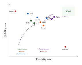
Proposition 18 (Pareto Frontier Characterisation).
For a fixed architecture and a quadratic approximation to both the stability loss and the plasticity gain , where is the regularisation strength, the Pareto frontier (Pareto) is a convex curve in the plane, traced by varying from (maximum plasticity, no stability) to (maximum stability, no plasticity).
Proof.
Computing the second derivative of with respect to along the frontier (eliminating ), we find for all , confirming concavity of as a function of . Equivalently, the frontier is a convex set when viewed as the region below the curve.
Example 12 (Quadratic Pareto Example).
For a concrete illustration, let and , so and . At (pure plasticity): , . At (pure stability): , . At (balanced): , .
The balanced point achieves , compared to for pure plasticity and for pure stability. The sum is maximised at , giving and , with sum . This shows that the optimal operating point is not the midpoint but is skewed toward the side with larger capacity constant.
Connections and Synthesis
Continual learning does not exist in isolation. It intersects deeply with memory management (24), alignment and fine-tuning (25), and reasoning (Adaptive Computation Time, Self-Refine). These connections are not superficial analogies; they are mathematical equivalences that allow us to transfer techniques, theorems, and intuitions across domains. This section makes these connections precise.
Continual Learning Meets Memory
The relationship between continual learning and memory management is the deepest of the three connections. At a high level, memory provides the mechanism by which a system resists forgetting, and continual learning provides the dynamics by which memory is tested.
| CL Concept | Memory Concept | Mathematical Link |
| Replay buffer | Hippocampal replay | episodic memory |
| Weight consolidation | Neocortical consolidation | synaptic strength |
| Task-specific adapters | Context-dependent retrieval | LoRA memory addressing |
| Catastrophic forgetting | Retroactive interference | overwriting |
| Progressive networks | Neurogenesis | New columns new neurons |
| Experience replay | Memory reconsolidation | Rehearsal reactivation |
| Knowledge distillation | Teaching consolidation | Soft labels schema formation |
| Sparse memory updates | Sparse coding in cortex | -hot population coding |
| Surprise-gated learning | Novelty detection | dopamine signal |
The correspondences in Table 3 are not merely poetic analogies; they reflect genuine mathematical equivalences. For instance, the correspondence between replay buffers and hippocampal replay is grounded in the fact that both implement the same operation: sampling from a stored distribution of past experiences and interleaving these samples with new data during learning. The Widrow–Hoff update rule used by Titans' neural memory (Definition 31) is the same learning rule that computational neuroscience models attribute to hippocampal place cells. Even the surprise-gated learning of Titans has a biological counterpart in the dopaminergic novelty signal that gates learning in the hippocampus.
Remark 22 (Memory–CL Duality).
Memory management and continual learning are dual perspectives on the same underlying problem. Memory management takes a static view: given a fixed computational budget, how should we organise storage to support retrieval? Continual learning takes a dynamic view: given a stream of experiences, how should we update our system to retain useful knowledge?
Formally, a memory system (Definition 20) with read/write operations is equivalent to a lifelong learning system (Definition 42) where:
The architecture includes the memory's addressing mechanism,
The hierarchical memory is the memory bank itself,
The learning rule is the write operation,
The memory update is the consolidation/eviction policy.
This duality explains why advances in one field immediately transfer to the other: the Titans architecture (Definition 31) is simultaneously a memory system and a continual learner.
Example 13 (CLS Theory as HSD).
McClelland et al.'s Complementary Learning Systems (CLS) theory [11] posits that the brain uses two complementary systems:
The hippocampus: fast-learning, episodic, sparse encoding. New experiences are stored rapidly with minimal interference.
The neocortex: slow-learning, semantic, distributed encoding. Knowledge is gradually consolidated through interleaved replay (during sleep).
In HSD terms, the hippocampus is level 1 (, every experience, low due to sparse coding) and the neocortex is level 2 (, periodic consolidation, high due to distributed representations). The memory update function is sleep consolidation, which transfers information from level 1 to level 2 through replay.
This mapping reveals why CLS theory is so successful: it naturally minimises the HSD forgetting bound. The hippocampus's sparse coding gives small ; the neocortex's slow learning gives small ; and the replay-based consolidation ensures that the large of the neocortex does not cause catastrophic forgetting because updates are small and interleaved with old patterns.
Continual Learning Meets Alignment
The standard alignment pipeline (Figure 2) consists of three stages: pretraining, supervised fine-tuning (SFT), and reinforcement learning from human feedback (RLHF). From the continual learning perspective, this is a three-task CL problem.
Proposition 19 (Alignment Is Continual Learning).
The alignment pipeline constitutes a three-task continual learning problem :
: Pretraining on web text (),
: SFT on instruction-response pairs (),
: RLHF/DPO alignment ().
The KL constraint in is an anti-forgetting mechanism: it prevents the aligned model from deviating too far from the SFT model, preserving the general capabilities acquired in tasks 1 and 2.
Proof.
We verify that the alignment pipeline satisfies the conditions of a CL problem (Definition 3). The three stages are trained sequentially on different data distributions (web text, instruction pairs, preference pairs). Each stage optimises a different loss function. The KL penalty in stage 3 has exactly the form of the EWC regulariser (Definition 12) with the Fisher replaced by the identity: (KL EWC) where is the Fisher information of the KL divergence, recovering the EWC objective with .
Corollary 2 (– Correspondence).
The DPO temperature parameter (Direct Preference Optimization) and the EWC regularisation strength (Definition 12) play equivalent mathematical roles. Specifically:
: maximum plasticity, the model ignores the reference and optimises reward freely (equivalent to in EWC);
: maximum stability, the model stays at the reference policy (equivalent to in EWC);
The optimal balances reward improvement against capability preservation, analogous to the optimal in EWC.
This correspondence suggests that techniques for tuning in CL (e.g., online cross-validation on a held-out buffer) can be directly applied to tuning in alignment, and vice versa.
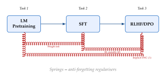
The – correspondence of Corollary 2 has immediate practical implications. In the alignment literature, there is extensive work on tuning : too small leads to reward hacking, too large leads to insufficient alignment. In the CL literature, there is parallel work on tuning : too small leads to catastrophic forgetting, too large leads to intransigence. The correspondence means that any technique for tuning one parameter can be directly translated to the other. For example, the “warm-up” strategy common in RLHF (starting with large and gradually decreasing) corresponds to starting with strong regularisation and gradually relaxing it, precisely the schedule proposed by [28] in the CL context.
Conversely, the CL insight that should be adaptive (different for different parameters, based on their Fisher information) suggests that in DPO should also be parameter-dependent: parameters that are more important for maintaining pretrained capabilities should be regularised more strongly, while parameters that can safely change should be regularised less. This idea, parameter-adaptive DPO, is a direct prediction of the CL–alignment connection that has not yet been explored in the alignment literature.
Continual Learning Meets Reasoning
The connection between continual learning and reasoning is more subtle but equally important.
Remark 23 (Reasoning as Intra-Task Continual Learning).
Adaptive Computation Time (ACT, Adaptive Computation Time) and self-refinement (Self-Refine) can be viewed as intra-task continual learning: the model iteratively refines its answer, and each refinement step is a “micro-task” where the model must improve on its previous output without losing the useful information already gathered.
More formally, consider a chain-of-thought reasoning process that generates intermediate states . At each step, the model must:
Remember relevant facts and intermediate conclusions (stability),
Incorporate new reasoning steps (plasticity),
Not regress on previously correct sub-conclusions (bounded forgetting).
This is precisely the stability–plasticity dilemma (Definition 7) operating at the timescale of a single inference, rather than across training epochs.
Test-Time Training (TTT) makes this connection explicit by literally performing gradient-based learning during inference, updating a subset of model parameters to adapt to the current input. From the CL perspective, TTT is a single-task continual learner that operates at inference time.
Key Idea.
The CL–Reasoning bridge. The connection between CL and reasoning suggests a powerful transfer of ideas. CL techniques designed to prevent forgetting across training epochs (EWC, replay) could be adapted to prevent “reasoning forgetting” within a single inference chain. Conversely, reasoning techniques designed to maintain coherence across steps (chain-of-thought verification, self-consistency) could inspire new CL methods that verify old-task performance during new-task learning. This bidirectional transfer is largely unexplored.
Open Problems
Despite the rapid progress surveyed in this chapter, fundamental questions remain unanswered. We highlight five that we consider most pressing.
Optimal CL architecture at 100B+ scale. Current CL methods have been validated at the 7B–13B parameter scale. How do they behave at 100B+? Does the increased capacity of larger models provide natural resistance to forgetting (as suggested by the capacity bound of Theorem 8), or do new failure modes emerge?
Forgetting in reasoning chains. When a continually-trained model loses knowledge, how does this affect multi-step reasoning? A forgotten fact at step 3 of a 10-step chain may cause cascading errors. Formal analysis of reasoning-chain fragility under forgetting is needed.
Theoretical limits of LoRA-based CL. LoRA-CL (Definition 23) has emerged as the dominant practical approach, yet its theoretical properties are poorly understood. What is the maximum number of tasks representable by rank- adapters before interference dominates? How does composition quality degrade with the number of composed adapters?
Continual RLHF. Human preferences evolve over time. A deployed model must continually align to shifting preferences without forgetting previously learned safety constraints. The interaction between reward model drift and policy forgetting is largely unexplored.
Multi-modal CL at scale. As shown in Multimodal and Federated Continual Learning, cross-modal forgetting amplifies the challenge. Scaling multimodal CL to systems with modalities (text, image, audio, video, code) introduces combinatorial cross-modal interference that current frameworks cannot address.
Conjecture 2 (CL Scaling Law).
The expected loss of a continually-trained model follows a power-law scaling relation: (Scaling LAW) where is the parameter count, is the number of tasks, are constants, captures the standard scaling benefit, and capture the forgetting overhead. The first term is the standard neural scaling law; the second term is the CL tax, the additional loss due to sequential training. For the CL tax to vanish as , we need , i.e., larger models must be more resistant to forgetting per task.
The critical insight is the exponent relationship: if , then the CL tax grows slower than the scaling benefit, and sufficiently large models can absorb an arbitrary number of tasks. If , forgetting eventually dominates regardless of scale.
Remark 24 (The Practitioner's Dilemma).
For the practitioner facing a concrete CL problem today, the open problems above may seem abstract. A more immediate question is: which method should I use? Based on the analysis in this chapter, we offer the following decision tree:
If task identity is available at inference time and storage is ample: use LoRA-CL (Definition 23). It provides zero forgetting by construction and is the simplest to implement.
If task identity is unavailable: use LoRA-CL with a learned router (combining Definition 23 and Definition 25).
If the task sequence is long () and storage is limited: consider CPT with replay (Definition 26) for domain adaptation or experience replay (Definition 17) for classification.
If online, streaming data with no task boundaries: use infinite cosine schedule (Definition 27) with replay.
If building a new architecture from scratch: incorporate neural memory (Definition 31 or Definition 34) to achieve CL as an emergent property rather than an add-on.
Full Taxonomy
We conclude the synthesis with a comprehensive taxonomy of all CL methods discussed in this chapter, visualised as a mind map that highlights both the categorical structure and the cross-connections.
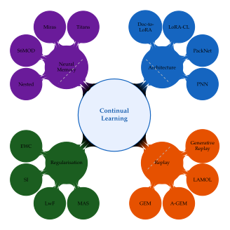
Historical Timeline
The story of continual learning is, in many ways, the story of how science repeatedly discovers, forgets, and rediscovers the problem of forgetting. The phenomenon was first documented rigorously in the 1880s, forgotten by the machine learning community for a century, rediscovered with alarm in the 1980s, and has since oscillated between periods of intense activity and relative neglect. We are currently in the most sustained period of progress, driven by the practical necessity of updating large language models without retraining from scratch.
Historical Note.
The Ebbinghaus inheritance (1885–1975). Hermann Ebbinghaus published Über das Gedächtnis in 1885 [9], establishing the exponential forgetting curve through meticulous self-experimentation with nonsense syllables. His key insight, that forgetting follows a predictable mathematical law, would not be fully appreciated by the machine learning community for over a century. Meanwhile, the psychologist Sebastian Leitner developed his spaced-repetition system in 1972 [10], showing that strategically timed rehearsal could dramatically extend retention, an idea that foreshadows modern experience replay.
Historical Note.
Adaptive Resonance and stability (1976–1988). Stephen Grossberg's Adaptive Resonance Theory (ART) [29] was the first neural network framework to explicitly address the stability–plasticity dilemma. ART networks solve the problem through architectural means: a vigilance parameter controls whether a new input is assimilated into an existing category (stability) or triggers the creation of a new category (plasticity). While ART networks were limited to relatively simple classification tasks, they established the principle that architecture matters for continual learning, a principle that PNN, PackNet, and modern adapter-based methods would independently rediscover.
The significance of Grossberg's contribution cannot be overstated. At a time when most connectionist researchers viewed learning as a monolithic process (present data, update weights, repeat) Grossberg recognised that the dynamics of learning matter as much as the objective. A system that learns too eagerly will overwrite its past; a system that learns too cautiously will fail to adapt. This insight, expressed mathematically through the stability–plasticity dilemma, remains the central challenge of continual learning forty years later.
Historical Note.
The catastrophic interference crisis (1989–1999). McCloskey and Cohen's 1989 paper [1] demonstrated that standard backpropagation networks exhibit catastrophic interference: training on new patterns almost completely destroys previously learned patterns. This finding was deeply troubling; it suggested that connectionist models were fundamentally incapable of the kind of incremental learning that biological systems perform effortlessly. Ratcliff (1990) confirmed the finding across multiple architectures. McClelland, McNaughton, and O'Reilly's landmark 1995 paper [11] proposed Complementary Learning Systems (CLS) theory: the brain solves catastrophic interference by maintaining two learning systems (hippocampus for fast episodic learning, neocortex for slow statistical learning) that interact through memory consolidation during sleep. French's 1999 review [2] surveyed a decade of failed solutions, concluding that “the problem of catastrophic forgetting remains unsolved.”
French's review is worth quoting directly: “Connectionist models, as currently implemented, are fundamentally unable to incrementally learn new information without catastrophically forgetting previously learned information.” This conclusion, while overly pessimistic in retrospect, accurately captured the state of the art at the turn of the millennium. The field entered a quiet period: catastrophic forgetting was treated as a known, unsolvable limitation of neural networks, and researchers either accepted it or worked on entirely different architectures (support vector machines, tree ensembles) that did not suffer from it.
Historical Note.
The deep learning awakening (2014–2017). Goodfellow et al. (2014) [30] revisited catastrophic forgetting in modern deep networks, finding that the problem persists, and is arguably worse, in deeper, more expressive architectures. This paper catalysed a wave of solutions: Kirkpatrick et al. (2017) introduced EWC [3], Zenke et al. (2017) introduced SI [31], Li and Hoiem (2017) introduced LwF [32], Lopez-Paz and Ranzato (2017) introduced GEM [33], and Rusu et al. (2016) introduced PNN [18]. Shin et al. (2017) [15] showed that generative replay, training a generative model to produce pseudo-examples of old tasks, could replace stored data entirely. In a single year, the four main CL paradigms (regularisation, replay, architecture, generative) were established.
Historical Note.
Consolidation and scaling (2018–2023). The period 2018–2023 saw consolidation of the theoretical foundations and early scaling to larger models. Schwarz et al. (2018) [28] introduced Progress & Compress. Chaudhry et al. (2019) [16] simplified GEM with A-GEM. Mallya and Lazebnik (2018) [19] showed that network pruning could create space for new tasks. Parisi et al. (2019) [4] and De Lange et al. (2021) [5] provided comprehensive surveys. Sun et al. (2020) [14] brought CL to language models with LAMOL. Hu et al. (2022) [34] introduced LoRA, which, while not designed for CL, would become the most important practical tool for parameter-efficient continual learning.
This consolidation period established two crucial insights. First, there is no single best CL method: the optimal approach depends on the scenario (task-incremental vs. class-incremental vs. domain-incremental), the resource constraints (memory budget, compute budget), and the nature of the tasks (similar vs. dissimilar). Second, parameter efficiency is a form of anti-forgetting: methods that update fewer parameters (either explicitly through masking or implicitly through low-rank constraints) consistently achieve better stability, even without any explicit regularisation. This insight would prove prophetic as LoRA emerged as the dominant practical tool.
Historical Note.
The LLM era (2024–2025). The deployment of large language models at scale has made continual learning an urgent industrial priority. Shi et al. (2024) [7] and Wang et al. (2023) [6] surveyed the emerging landscape. Bell et al. (2025) [8] outlined the future of CL for foundation models. On the methods front, 2025 has been remarkably productive: Liu et al. introduced C-CLIP [21] for vision-language CL, Singh et al. proposed the infinite cosine schedule [24], Behrouz et al. developed both Titans [35] and Miras [36] for neural memory, Liu et al. introduced S6MOD [26] for multi-head state-space memory, Behrouz et al. proposed nested learning [37], Yi et al. developed MultiFCL [27] for federated settings, and Charakorn et al. introduced Doc-to-LoRA [22] for document-conditioned adaptation. The field has shifted from “can we prevent forgetting?” to “how do we build systems that learn and remember at scale?”
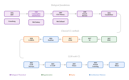
Exercises
The exercises below span the full range of topics covered in this chapter, from foundational calculations to open-ended design problems. Exercises 1–6 test understanding of the core CL mechanisms (forgetting curves, Bayesian CL, EWC, Fisher information, GEM, reservoir sampling). Exercises 7–10 address LLM-specific methods (LAMOL, PNN, LoRA, Doc-to-LoRA). Exercises 11–18 explore the advanced topics of continual pre-training, learning rate scheduling, sparse memory, Titans, Miras, S6MOD, and nested learning. Exercises 19–21 cover diffusion models, C-CLIP, and federated CL. Exercises 22–26 probe the unified mathematical framework: knowledge capacity, HSD bounds, Pareto frontiers, alignment connections, and scaling laws. The final four exercises (27–30) are more open-ended, connecting CL to biology, online learning theory, compositionality, and system design.
Exercise 2 (Ebbinghaus Curve Analysis).
The Ebbinghaus forgetting curve (Definition 1) models retention as where is the memory strength.
Compute for with day. Express your answers to three decimal places. At what time is retention reduced to ?
Suppose each rehearsal multiplies the memory strength by a factor of (so after rehearsals, ). With and day, how many rehearsals are needed to maintain ?
The power-law forgetting model posits for some [38]. Find the that matches the exponential model at day (i.e., ). Plot both curves for and discuss which predicts more forgetting at long timescales.
Exercise 3 (Bayesian Continual Learning Derivation).
Consider the Bayesian CL framework of Definition 6.
Starting from a Gaussian prior , derive the sequential posterior after three tasks with Gaussian likelihoods . Show that the posterior after task 3 is Gaussian with precision .
Verify that the posterior mean after task is . Interpret this as a precision-weighted average of task-specific optima.
Show that the EWC objective (Definition 12) with diagonal Fisher is recovered when: (i) the posterior at each step is approximated as diagonal Gaussian, and (ii) the Fisher information replaces the Hessian . What information is lost in this approximation?
Exercise 4 (EWC Analytical Example).
Consider a model with two parameters . Task 0 has optimum with Fisher . Task 1 has loss .
Write the EWC objective for task 1 with regularisation strength . Find the closed-form optimal .
Plot the trajectory of as varies from to in the plane. Show that it traces a curve from to .
Compute the limits: and . For what value of is the forgetting on task 0 equal to the loss on task 1? Interpret the role of the asymmetric Fisher ().
Exercise 5 (Fisher Information Computation).
For a single-hidden-layer neural network with ReLU activation and mean-squared-error loss, derive the diagonal Fisher information matrix for the output layer weights . Show that where is the -th hidden activation.
Argue that parameters connected to high-variance hidden units have larger Fisher information. What does this imply for EWC: which parameters are most protected from modification?
For a large language model with vocabulary size , show that the per-parameter Fisher for the output embedding matrix scales as . Why does this make EWC less effective for protecting the output layer of LLMs?
Exercise 6 (GEM Projection Geometry).
In GEM (Definition 16), the gradient is projected to satisfy for all past tasks .
Consider tasks in . The current gradient is and the stored gradient is . Compute the GEM-projected gradient by solving the constrained QP: subject to .
What happens when (i.e., )? Show that in this case, the projection is the identity: . Interpret this geometrically.
Compare GEM to A-GEM (Definition 19). A-GEM uses a single randomly sampled reference gradient instead of all past gradients. For tasks, estimate the computational savings of A-GEM over GEM per update step. Under what conditions might A-GEM's approximation quality degrade significantly?
Exercise 7 (Reservoir Sampling).
A replay buffer of size is maintained using reservoir sampling (Proposition 6) over a stream of examples.
Prove that after processing all items, each item is in the buffer with probability exactly . [Hint: Use induction. When item arrives, it replaces a random buffer element with probability .]
Compute the expected number of replacement operations after processing all items. Show that this equals where is the -th harmonic number. For and , estimate this value.
Standard reservoir sampling does not guarantee class balance. Design a class-balanced reservoir sampling algorithm for classes that maintains exactly examples per class (assuming divides ). Prove that your algorithm maintains uniform probability within each class.
Exercise 8 (LAMOL Pseudo-Rehearsal Quality).
In LAMOL (Definition 18), the language model generates pseudo-examples of previous tasks. Let denote the quality degradation per generation step (i.e., each re-generation reduces quality by a fraction ).
After tasks, pseudo-examples of task 1 have been regenerated times. Show that the quality factor is . If is constant, simplify to .
Under what condition on does converge to zero as ? Show that for any , the quality eventually drops below any threshold after tasks. For and , compute .
Propose a mitigation strategy that uses a small replay buffer of real examples alongside LAMOL's generated examples. Argue informally that the quality degradation is bounded below by the quality of the real examples, preventing .
Exercise 9 (PNN Parameter Count).
A Progressive Neural Network (Definition 20) starts with an initial network of layers, each with width . Each new task adds a new column with lateral connections to all previous columns.
Derive the exact parameter count after tasks. Show that the total is for fully connected layers (accounting for both within-column and lateral-connection weights). Simplify.
Compare to the cost of training independent networks of the same architecture: . What is the ratio ? For , compute this ratio.
For , , and (a moderate Transformer), compute the total parameter count. Compare to the 7B parameters of LLaMA-2-7B. At what value of does PNN exceed the 7B threshold? Discuss the scalability implications.
Exercise 10 (LoRA Storage Analysis).
Consider LoRA adapters (Definition 2, Definition 23) applied to a LLaMA-2-7B model with Transformer layers, hidden dimension , and LoRA rank . Adapters are applied to the query and value projection matrices () in each layer.
Compute the total number of trainable parameters per adapter. Each adapter adds matrices and per target matrix. Express your answer as a fraction of the full model size.
In fp16 storage (2 bytes per parameter), how many task-specific adapters can be stored in 1,GB?
Compare the storage efficiency of LoRA-CL to PackNet (Definition 21), which stores a binary mask (1 bit per parameter) per task. For what values of LoRA rank is LoRA-CL more storage-efficient than PackNet?
Exercise 11 (Doc-to-LoRA Hypernetwork).
In Doc-to-LoRA (Definition 24), a hypernetwork maps documents to LoRA adapter weights, where is the adapter parameter count.
For the hypernetwork to be capable of producing any adapter weight vector, it must have at least output dimensions. If the hypernetwork is a Transformer with hidden dimension and the adapter has parameters, what is the minimum for the final linear projection to be surjective onto ? What does this imply about the hypernetwork's size relative to the adapter?
Describe a cross-attention architecture for the hypernetwork where the document tokens serve as keys/values and learnable query tokens generate the adapter weights. What are the computational advantages over a simple MLP hypernetwork?
Estimate the FLOPs cost of running the hypernetwork for a 512-token document with and a single cross-attention layer. Compare to the FLOPs of a single forward pass through the LLaMA-2-7B model.
Exercise 12 (CPT Data Mixing).
Continual pre-training (Definition 26) mixes new-domain data with replay data at ratio .
Model forgetting as , where is the forgetting constant and is the transfer benefit of new data on old tasks ( indicates positive transfer). Derive this bound from a first-order approximation of the loss landscape.
Find the optimal mixing ratio that minimises subject to achieving at least a fraction of the maximum new-task performance. Express in terms of , , and .
The empirical recommendation is (90% new data, 10% replay) [7]. Under what conditions on and does this match your optimal ?
Exercise 13 (Learning Rate and Forgetting).
The learning-rate forgetting bound (Theorem 5) states that forgetting is proportional to the product of learning rate and gradient magnitude.
Starting from , derive the first-order approximation: . When does new-task training help old tasks (negative forgetting)?
Consider a loss landscape with condition number where and are the largest and smallest eigenvalues of the Hessian. Compare the forgetting after one epoch for versus . What role does the condition number play?
The infinite cosine schedule (Definition 27) bounds the instantaneous learning rate by . Show that this implies a per-step forgetting bound of via Cauchy–Schwarz.
Exercise 14 (Infinite Cosine Schedule).
The infinite cosine schedule (Definition 27) defines where is the period.
For , , and steps, write out and plot it for (three complete cycles). Mark the points where and .
Compute the time-averaged learning rate over one cycle: . Show that .
At which points in the cosine cycle is the model most plastic (able to learn new patterns)? At which points is it most stable (resistant to forgetting)? Argue that the cosine schedule provides a natural alternation between “learning phases” and “consolidation phases” within each cycle.
Exercise 15 (Sparse Memory Layer Analysis).
A sparse memory layer (Definition 28) with memory slots and top- activation uses a -hot addressing scheme.
After update steps, each activating out of slots uniformly at random, what fraction of memory slots have been modified at least once? Express as a function of , , and .
The probability that a specific slot has not been modified after steps is . For , , and , compute this probability. What does it tell us about the memory's forgetting behaviour?
In the Sparse Memory Layer design (Definition 28), approximately 11% of parameters participate in any given forward pass, while 89% remain unchanged. Verify this by computing for typical values (, ) and explain why this sparsity pattern provides natural anti-forgetting protection (Proposition 13).
Exercise 16 (Titans Surprise Mechanism).
The Titans architecture (Definition 31) uses surprise (Definition 30) to gate memory updates.
The Titans memory update is . Show that for a linear memory with loss , the update becomes . Recognise this as the Widrow–Hoff (LMS) online learning rule.
The surprise is high when the current input is poorly predicted by existing memory. Argue that surprise is a natural novelty detector: familiar inputs (seen during previous tasks) have low surprise, while novel inputs (from a new task) have high surprise. How does this relate to the stability–plasticity trade-off?
Design a forget gate that uses surprise: , where for learnable . What is the effect of when surprise is high versus low? Relate to the biological concept of reconsolidation.
Exercise 17 (Miras Equivalence).
The Miras framework (Definition 32) establishes an equivalence between Test-Time Memory (TTM) and linear attention.
Write the TTM update rule: given query , key , value , the memory state is and the output is . Expand explicitly as a sum over past inputs.
Write the linear attention recurrence: and , where is a feature map. Show that with (identity), this is identical to the TTM update from part (a).
Show the full Miras equivalence: any TTM with update rule is equivalent to a gated linear attention mechanism with decay factor . [Hint: Unroll the recurrence.]
Discuss the practical implication: if TTM and linear attention are equivalent, then advances in efficient attention (e.g., hardware optimisations for linear attention) directly benefit continual learning systems, and vice versa.
Exercise 18 (S6MOD Multi-Head States).
The S6MOD architecture (Definition 33) uses independent state heads, each with state dimension .
Compute the total state size for a model with layers, heads per layer, and state dimensions per head. Express in number of parameters and in MB (fp16).
Compare this to a single-head SSM with the same total state dimension per layer. What are the theoretical advantages of the multi-head decomposition in terms of (i) parallel computation and (ii) expressiveness for multi-task learning?
Design a routing function that assigns different heads to different tasks: where . Argue that this creates a form of sparse memory allocation that naturally reduces cross-task interference.
Exercise 19 (Nested Learning Convergence).
Nested learning (Definition 34) assigns different learning rates to different levels: level uses rate for some constant .
For level 2 with , show that after steps, the parameter update is . If are i.i.d. with mean and variance , show that converges to and the variance of the estimate decreases as , i.e., level 2 converges to the time-averaged gradient.
Define the effective number of samples for level as the number of steps needed to achieve variance in the gradient estimate, where is the level dimension. Express this in terms of and .
Relate nested learning to Polyak averaging (exponential moving average of parameters). Show that if for small , the multi-level scheme approximates a hierarchy of EMA with decay rates .
Exercise 20 (Diffusion Model Forgetting).
A diffusion model is trained on landscapes (task 0), achieving . It is then fine-tuned on portraits (task 1). After fine-tuning, (landscapes) and (portraits).
Compute the diffusion forgetting score (Definition 36). Is this severe forgetting?
After applying noise-level-aware EWC (Proposition 15) with , the landscape FID improves to while portrait FID degrades slightly to . Compute the new forgetting score and the forgetting–performance trade-off ratio .
With concept-specific LoRA (Definition 37), the landscape FID remains at (exact zero forgetting) and portrait FID is . Explain why LoRA achieves zero forgetting. What is the practical cost of this guarantee (i.e., what assumption must hold at inference time)?
Exercise 21 (C-CLIP Benchmark Analysis).
In the C-CLIP evaluation (Definition 39), LoRA-CL achieves average accuracy across 10 datasets, while the best individual method (varying per dataset) averages . Full fine-tuning achieves .
Compute the relative improvement of LoRA-CL over full fine-tuning: . Compute the gap to the best method: . Verify that the gap satisfies (LORA Dominance).
If LoRA uses rank on a CLIP ViT-B/16 with , compute the parameter ratio for adapters on Q and V projections across layers.
Why does structural isolation (freezing the base model and only training adapters) outperform regularisation-based methods (EWC, SI) in the VLCL setting? Relate your answer to the stability–plasticity analysis of Definition 7 and the cross-modal forgetting bound of Proposition 17.
Exercise 22 (Federated Continual Learning Communication).
Consider a MultiFCL system (Definition 41) with clients, model size parameters, and scales.
In standard federated averaging (FedAvg), each communication round transmits parameters per client (both directions). The total communication cost per round is (in parameter units). In MultiFCL, only scales and are communicated (scale is local). If scale 1 has parameters and scale 2 has parameters, compute the communication cost per round.
Compute the communication overhead of MultiFCL relative to FedAvg: . Under what conditions is MultiFCL cheaper than FedAvg? [Hint: MultiFCL communicates more frequently for scale 1 but less for scale 2.]
The MultiFCL framework assumes that clients have heterogeneous task sequences. Under what conditions on the similarity between client task distributions does federated aggregation actually help (positive transfer) versus hurt (negative transfer)? Relate to the task similarity measure of Definition 8.
Exercise 23 (Knowledge Capacity Calculations).
Use the knowledge capacity framework of Definition 43.
Compute in bits for: (i) a 7B-parameter model in fp16, (ii) a 70B-parameter model in fp16, (iii) a 7B-parameter model in int4 quantisation. Express each in gigabytes.
If each task requires bits of unique information, how many tasks can each model from part (a) accommodate with zero forgetting (Theorem 8)?
A LoRA adapter with rank on Q and V projections across layers of a model has how many bits (in fp16)? How many adapters fit within the “leftover” capacity of a 7B model that has used 80% of its raw capacity for pretrained knowledge?
Exercise 24 (HSD Forgetting Bound Computation).
Consider a 3-level HSD architecture (Definition 44) with the following parameters:
| Level | ||||
| 1 (fast/dense) | 1.0 | 100 | 0.1 | 0.01 |
| 2 (hybrid) | 0.1 | 10 | 1.0 | 0.005 |
| 3 (slow/sparse) | 0.001 | 1 | 10.0 | 0.001 |
Compute the per-level forgetting contributions and the total forgetting bound . Which level contributes most?
Compute the ratio between the highest and lowest per-level contributions. Show that the sparse, slow level (level 3) contributes roughly less forgetting than the dense, fast level (level 1), despite having a higher condition number.
Suppose you have a budget of total forgetting. Formulate and solve the optimisation problem: subject to , where decreases with . Show that the optimal allocation concentrates updates at the level with the smallest ratio.
Exercise 25 (Pareto Frontier Analysis).
Use the stability–plasticity model of Proposition 18 with and where and .
Eliminate to derive the Pareto frontier as an explicit curve . [Hint: Solve for and substitute into .]
Show that everywhere on the frontier, confirming convexity of the feasible region.
At the Pareto-optimal point, the marginal cost of additional stability equals the marginal benefit of plasticity. Find the that satisfies . Interpret this as the “balanced” CL operating point.
Exercise 26 (Alignment as Continual Learning).
Map the three-stage alignment pipeline to a CL problem (Proposition 19).
Write out the loss functions for the three tasks: (pretraining), (SFT), and (DPO with temperature ). Identify the data distribution for each task and explain why they constitute a non-stationary sequence.
Show the – correspondence (Corollary 2) explicitly. Starting from the DPO loss , perform a second-order Taylor expansion around and identify the EWC-like quadratic penalty.
How would the analysis change for GRPO (Group Relative Policy Optimization), which uses a group of sampled responses instead of paired preferences? Is the – correspondence still valid?
Exercise 27 (CL Scaling Law).
Consider the conjectured CL scaling law (Conjecture 2): .
Show that for the CL tax (second term) to decrease with model size for any fixed , we need . What happens when ? Interpret physically.
The condition for CL to be preferable to retraining from scratch is . This simplifies to , which is never satisfied. Resolve this apparent paradox by introducing a data efficiency term: CL uses total tokens, while retraining uses . Modify the scaling law to account for the data savings and find the break-even condition.
Design an experiment to estimate , , and empirically. You have access to models of sizes and can run task sequences of length . Describe the experimental protocol, including how to disentangle the scaling exponents.
Exercise 28 (Biological Continual Learning).
The brain is the most successful continual learner known. This exercise explores the mathematical parallels.
Map the brain's memory systems to the HSD framework (Definition 44). Identify the biological counterparts of: (i) level 1 (fast, dense), (ii) level 2 (hybrid), (iii) level 3 (slow, sparse). What are the biological analogues of , , and ?
Estimate the brain's knowledge capacity using Definition 43. The brain has approximately synapses, each storing an estimated 4.7 bits of information [11]. Compare to a 70B-parameter LLM in fp16.
Estimate the number of “tasks” a human learns in a lifetime. If we define a task as a coherent skill or knowledge domain (e.g., “riding a bicycle,” “algebra,” “a friend's name”), a rough estimate is – tasks over 80 years. Using the capacity from part (b) and the information bound (Theorem 8), what is the maximum information per task? Is this consistent with the observation that humans forget most of what they experience?
Exercise 29 (Online Learning Regret for CL).
Continual learning can be framed as an online learning problem, where the learner sees one task per round and accumulates regret.
Define the CL regret after tasks as , where is the model's parameters when evaluated on task and is the per-task optimum. How does this differ from the standard forgetting metric (Definition 9)?
For online gradient descent (OGD) with learning rate and convex losses, the classical bound is . Verify this by computing the regret bound for quadratic losses with .
Can EWC achieve sublinear regret? Argue that EWC with optimal achieves regret for quadratic losses by showing that the EWC update is equivalent to OGD with a preconditioned step. Under what conditions on the Fisher matrices does this hold?
Exercise 30 (Compositionality and Routing).
Consider a LoRA-based compositional CL system (Definition 25) with adapters, each of rank , applied to a model with hidden dimension .
Compute the total parameter count for adapters with and , applied to Q and V projections in each of layers. Express as a percentage of the 7B base model.
A routing function selects adapter weights based on the input . Compute the FLOPs cost of routing (one matrix-vector multiply plus softmax) relative to a single adapter's forward pass ().
Two adapters compose without interference if their column spaces are orthogonal: . For rank- adapters in , what is the maximum number of pairwise orthogonal adapters? Relate to the maximum number of interference-free tasks. What happens when the number of tasks exceeds this limit?
Exercise 31 (Open Problem: Designing an HSD System).
This capstone exercise asks you to design a complete HSD-based continual learning system for a 7B-parameter language model.
Design a 3-level HSD architecture. Specify: itemize
Level 1: which parameters, update rule, and update frequency,
Level 2: adapter configuration (rank, target modules),
Level 3: which parameters are frozen and under what conditions (if any) they may be updated. itemize Justify your choices using the HSD forgetting bound (Theorem 9).
Using the parameters from your design, estimate the forgetting bound after 100 tasks. Compute , , , and for each level (you may estimate from typical Hessian spectral norms reported in the literature).
Compare your design to Titans (Definition 31). Identify at least two specific differences and argue which design would achieve lower forgetting and why.
Propose a concrete experiment to validate your design. Specify: the base model, the task sequence (at least 10 tasks from different domains), the evaluation metrics (including both per-task accuracy and cross-task transfer), and the baselines you would compare against. Estimate the computational cost in GPU-hours.
Key Idea.
The arc of continual learning. This chapter has traced a long arc, from Ebbinghaus's forgetting curve through Grossberg's stability–plasticity dilemma, from the catastrophic interference crisis to the modern era of LoRA adapters and neural memory systems. The central insight, distilled through two centuries of research, is deceptively simple: learning and remembering are not opposing forces but complementary aspects of a single process. The systems that learn best are those that remember selectively, and the systems that remember best are those that continue to learn.
The unified framework of A Unified Mathematical Framework provides the mathematical language to make this insight precise. The HSD architecture shows that the key to continual learning is not any single technique, not regularisation alone, not replay alone, not architectural isolation alone, but the hierarchical combination of all three, operating at different timescales and different levels of abstraction. The ideal continual learner, if it exists, will be a system that seamlessly integrates fast adaptation with slow consolidation, sparse task-specific memory with dense shared representations, and online learning with periodic reflection.
We do not yet have such a system. But the mathematical foundations developed in this chapter, the information-theoretic bounds, the forgetting inequalities, the Pareto characterisations, and the connections to memory, alignment, and reasoning, provide the tools to guide the search.
References
-
Catastrophic Interference in Connectionist Networks: The Sequential Learning Problem
BibTeX
@inproceedings{mccloskey1989catastrophic, title={Catastrophic Interference in Connectionist Networks: The Sequential Learning Problem}, author={McCloskey, Michael and Cohen, Neal J}, booktitle={Psychology of Learning and Motivation}, volume={24}, pages={109--165}, publisher={Academic Press}, year={1989} }Conference paper
-
Catastrophic Forgetting in Connectionist Networks
BibTeX
@article{french1999catastrophic, title={Catastrophic Forgetting in Connectionist Networks}, author={French, Robert M}, journal={Trends in Cognitive Sciences}, volume={3}, number={4}, pages={128--135}, year={1999} }Journal article
-
Overcoming Catastrophic Forgetting in Neural Networks
BibTeX
@article{kirkpatrick2017ewc, title={Overcoming Catastrophic Forgetting in Neural Networks}, author={Kirkpatrick, James and Pascanu, Razvan and Rabinowitz, Neil and Veness, Joel and Desjardins, Guillaume and Rusu, Andrei A and Milan, Kieran and Quan, John and Ramalho, Tiago and Grabska-Barwinska, Agnieszka and Hassabis, Demis and Clopath, Claudia and Kumaran, Dharshan and Hadsell, Raia}, journal={Proceedings of the National Academy of Sciences}, volume={114}, number={13}, pages={3521--3526}, year={2017} }Journal article
-
Continual Lifelong Learning with Neural Networks: A Review
BibTeX
@article{parisi2019continual, title={Continual Lifelong Learning with Neural Networks: A Review}, author={Parisi, German I and Kemker, Ronald and Part, Jose L and Kanan, Christopher and Wermter, Stefan}, journal={Neural Networks}, volume={113}, pages={54--71}, year={2019} }Journal article
-
A Continual Learning Survey: Defying Forgetting in Classification Tasks
BibTeX
@article{delange2021continual, title={A Continual Learning Survey: Defying Forgetting in Classification Tasks}, author={De Lange, Matthias and Aljundi, Rahaf and Masana, Marc and Parisot, Sarah and Jia, Xu and Leonardis, Ale{\v{s}} and Slabaugh, Gregory and Tuytelaars, Tinne}, journal={IEEE Transactions on Pattern Analysis and Machine Intelligence}, volume={44}, number={7}, pages={3366--3385}, year={2021} }Journal article
-
A Comprehensive Survey of Continual Learning: Theory, Method and Application
BibTeX
@article{wang2023comprehensive_cl_survey, title={A Comprehensive Survey of Continual Learning: Theory, Method and Application}, author={Wang, Liyuan and Zhang, Xingxing and Su, Hang and Zhu, Jun}, journal={IEEE Transactions on Pattern Analysis and Machine Intelligence}, year={2024} }Journal article
-
Continual Learning of Large Language Models: A Comprehensive Survey
BibTeX
@article{shi2024continual_llm_survey, title={Continual Learning of Large Language Models: A Comprehensive Survey}, author={Shi, Haizhou and Xu, Zihao and Wang, Hengyi and Qin, Weiyi and Wang, Wenyuan and Wang, Yibin and Wang, Hao}, journal={arXiv preprint arXiv:2404.16789}, year={2024} }Journal article
-
The Future of Continual Learning in the Era of Foundation Models: Three Key Directions
BibTeX
@article{bell2025future_cl, title={The Future of Continual Learning in the Era of Foundation Models: Three Key Directions}, author={Bell, Jack and Quarantiello, Luigi and Coleman, Eric Nuertey and Li, Lanpei and Li, Malio and Madeddu, Mauro and Piccoli, Elia and Lomonaco, Vincenzo}, journal={arXiv preprint arXiv:2506.03320}, year={2025} }Journal article
-
Uber das Gedachtnis: Untersuchungen zur experimentellen Psychologie
BibTeX
@book{ebbinghaus1885memory, title={{\"U}ber das {G}ed{\"a}chtnis: {U}ntersuchungen zur experimentellen {P}sychologie}, author={Ebbinghaus, Hermann}, year={1885}, publisher={Duncker \& Humblot}, address={Leipzig} }Book
-
So Lernt Man Lernen: Der Weg zum Erfolg (Learning to Learn)
BibTeX
@article{leitner1972learn, title={So Lernt Man Lernen: Der Weg zum Erfolg ({Learning to Learn})}, author={Leitner, Sebastian}, year={1972}, publisher={Herder} }Journal article
-
Why There Are Complementary Learning Systems in the Hippocampus and Neocortex: Insights from the Successes and Failures of Connectionist Models of Learning and Memory
BibTeX
@article{mcclelland1995cls, title={Why There Are Complementary Learning Systems in the Hippocampus and Neocortex: Insights from the Successes and Failures of Connectionist Models of Learning and Memory}, author={McClelland, James L and McNaughton, Bruce L and O'Reilly, Randall C}, journal={Psychological Review}, volume={102}, number={3}, pages={419--457}, year={1995} }Journal article
-
What Learning Systems Do Intelligent Agents Need? Complementary Learning Systems Theory Updated
BibTeX
@article{kumaran2016learning, title={What Learning Systems Do Intelligent Agents Need? {C}omplementary Learning Systems Theory Updated}, author={Kumaran, Dharshan and Hassabis, Demis and McClelland, James L}, journal={Trends in Cognitive Sciences}, volume={20}, number={7}, pages={512--534}, year={2016} }Journal article
-
Random Sampling with a Reservoir
BibTeX
@article{vitter1985reservoir, title={Random Sampling with a Reservoir}, author={Vitter, Jeffrey S}, journal={ACM Transactions on Mathematical Software}, volume={11}, number={1}, pages={37--57}, year={1985} }Journal article
-
LAMOL: LAnguage MOdeling for Lifelong Language Learning
BibTeX
@inproceedings{sun2020lamol, title={{LAMOL}: {LA}nguage {MO}deling for Lifelong Language Learning}, author={Sun, Fan-Keng and Ho, Cheng-Hao and Lee, Hung-Yi}, booktitle={International Conference on Learning Representations (ICLR)}, year={2020} }Conference paper
-
Continual Learning with Deep Generative Replay
BibTeX
@inproceedings{shin2017continual_generative, title={Continual Learning with Deep Generative Replay}, author={Shin, Hanul and Lee, Jung Kwon and Kim, Jaehong and Kim, Jiwon}, booktitle={Advances in Neural Information Processing Systems (NeurIPS)}, year={2017} }Conference paper
-
Efficient Lifelong Learning with A-GEM
BibTeX
@inproceedings{chaudhry2019agem, title={Efficient Lifelong Learning with {A-GEM}}, author={Chaudhry, Arslan and Ranzato, Marc'Aurelio and Rohrbach, Marcus and Elhoseiny, Mohamed}, booktitle={International Conference on Learning Representations (ICLR)}, year={2019} }Conference paper
-
Distilling the Knowledge in a Neural Network
BibTeX
@inproceedings{hinton2015distilling, title={Distilling the Knowledge in a Neural Network}, author={Hinton, Geoffrey and Vinyals, Oriol and Dean, Jeff}, booktitle={NIPS Deep Learning and Representation Learning Workshop}, year={2015} }Conference paper
-
Progressive Neural Networks
BibTeX
@inproceedings{rusu2016pnn, title={Progressive Neural Networks}, author={Rusu, Andrei A and Rabinowitz, Neil C and Desjardins, Guillaume and Sober, Hubert and Kavukcuoglu, Koray and Hadsell, Raia}, booktitle={arXiv preprint arXiv:1606.04671}, year={2016} }Conference paper
-
PackNet: Adding Multiple Tasks to a Single Network by Iterative Pruning
BibTeX
@inproceedings{mallya2018packnet, title={{PackNet}: Adding Multiple Tasks to a Single Network by Iterative Pruning}, author={Mallya, Arun and Lazebnik, Svetlana}, booktitle={Proceedings of the IEEE Conference on Computer Vision and Pattern Recognition (CVPR)}, year={2018} }Conference paper
-
Piggyback: Adapting a Single Network to Multiple Tasks by Learning to Mask Weights
BibTeX
@article{mallya2018piggyback, title={Piggyback: Adapting a Single Network to Multiple Tasks by Learning to Mask Weights}, author={Mallya, Arun and Davis, Dillon and Lazebnik, Svetlana}, journal={Proceedings of the European Conference on Computer Vision (ECCV)}, year={2018} }Journal article
-
C-CLIP: Continual Learning for Vision-Language Models with LoRA
BibTeX
@inproceedings{liu2025cclip, title={{C-CLIP}: Continual Learning for Vision-Language Models with {LoRA}}, author={Liu, Yanming and others}, booktitle={International Conference on Learning Representations (ICLR)}, year={2025} }Conference paper
-
Doc-to-LoRA: Learning to Instantly Internalize Contexts
BibTeX
@article{charakorn2026doc_to_lora, title={{Doc-to-LoRA}: Learning to Instantly Internalize Contexts}, author={Charakorn, Rujikorn and Cetin, Edoardo and Uesaka, Shinnosuke and Lange, Robert Tjarko}, journal={arXiv preprint arXiv:2602.15902}, year={2026} }Journal article
-
Model-Agnostic Meta-Learning for Fast Adaptation of Deep Networks
BibTeX
@article{finn2017maml, title={Model-Agnostic Meta-Learning for Fast Adaptation of Deep Networks}, author={Finn, Chelsea and Abbeel, Pieter and Levine, Sergey}, journal={Proceedings of the International Conference on Machine Learning (ICML)}, year={2017} }Journal article
-
Beyond Cosine Decay: On the Effectiveness of Infinite Learning Rate Schedule for Continual Pre-Training
BibTeX
@article{singh2025beyond_cosine, title={Beyond Cosine Decay: On the Effectiveness of Infinite Learning Rate Schedule for Continual Pre-Training}, author={Singh, Vaibhav and Janson, Paul and Mehrbod, Paria and Ibrahim, Adam and Rish, Irina and Belilovsky, Eugene and Th{\'e}rien, Benjamin}, journal={arXiv preprint arXiv:2503.02844}, year={2025} }Journal article
-
Continual Learning via Sparse Memory Finetuning
BibTeX
@article{lin2025sparse_memory, title={Continual Learning via Sparse Memory Finetuning}, author={Lin, Jessy and Zettlemoyer, Luke and Ghosh, Gargi and Yih, Wen-Tau and Markosyan, Aram and Berges, Vincent-Pierre and O{\u{g}}uz, Barlas}, journal={arXiv preprint arXiv:2510.15103}, year={2025} }Journal article
-
Enhancing Online Continual Learning with Plug-and-Play State Space Model and Class-Conditional Mixture of Discretization
BibTeX
@inproceedings{liu2024s6mod, title={Enhancing Online Continual Learning with Plug-and-Play State Space Model and Class-Conditional Mixture of Discretization}, author={Liu, Sihao and Yang, Yibo and Li, Xiaojie and Clifton, David A. and Ghanem, Bernard}, booktitle={Proceedings of the IEEE/CVF Conference on Computer Vision and Pattern Recognition (CVPR)}, year={2025} }Conference paper
-
MultiFCL: Multi-Scale Federated Continual Learning
BibTeX
@inproceedings{yi2025multifcl, title={{MultiFCL}: Multi-Scale Federated Continual Learning}, author={Yi, Jiaqi and others}, booktitle={Advances in Neural Information Processing Systems (NeurIPS)}, year={2025} }Conference paper
-
Progress & Compress: A Scalable Framework for Continual Learning
BibTeX
@article{schwarz2018progress, title={Progress \& Compress: A Scalable Framework for Continual Learning}, author={Schwarz, Jonathan and Czarnecki, Wojciech and Luketina, Jelena and Grabska-Barwinska, Agnieszka and Teh, Yee Whye and Pascanu, Razvan and Hadsell, Raia}, journal={Proceedings of the International Conference on Machine Learning (ICML)}, year={2018} }Journal article
-
Adaptive Pattern Classification and Universal Recoding: I. Parallel Development and Coding of Neural Feature Detectors
BibTeX
@article{grossberg1976art, title={Adaptive Pattern Classification and Universal Recoding: {I}. Parallel Development and Coding of Neural Feature Detectors}, author={Grossberg, Stephen}, journal={Biological Cybernetics}, volume={23}, pages={121--134}, year={1976} }Journal article
-
An Empirical Investigation of Catastrophic Forgetting in Gradient-Based Neural Networks
BibTeX
@article{goodfellow2014empirical, title={An Empirical Investigation of Catastrophic Forgetting in Gradient-Based Neural Networks}, author={Goodfellow, Ian J and Mirza, Mehdi and Xiao, Da and Courville, Aaron and Bengio, Yoshua}, journal={arXiv preprint arXiv:1312.6211}, year={2014} }Journal article
-
Continual Learning Through Synaptic Intelligence
BibTeX
@inproceedings{zenke2017si, title={Continual Learning Through Synaptic Intelligence}, author={Zenke, Friedemann and Poole, Ben and Ganguli, Surya}, booktitle={Proceedings of the International Conference on Machine Learning (ICML)}, year={2017} }Conference paper
-
Learning without Forgetting
BibTeX
@inproceedings{li2017lwf, title={Learning without Forgetting}, author={Li, Zhizhong and Hoiem, Derek}, booktitle={IEEE Transactions on Pattern Analysis and Machine Intelligence}, volume={40}, number={12}, pages={2935--2947}, year={2018} }Conference paper
-
Gradient Episodic Memory for Continual Learning
BibTeX
@inproceedings{lopez2017gem, title={Gradient Episodic Memory for Continual Learning}, author={Lopez-Paz, David and Ranzato, Marc'Aurelio}, booktitle={Advances in Neural Information Processing Systems (NeurIPS)}, year={2017} }Conference paper
-
LoRA: Low-Rank Adaptation of Large Language Models
BibTeX
@article{hu2022lora, title={{LoRA}: Low-Rank Adaptation of Large Language Models}, author={Hu, Edward J and Shen, Yelong and Wallis, Phillip and Allen-Zhu, Zeyuan and Li, Yuanzhi and Wang, Shean and Wang, Lu and Chen, Weizhu}, journal={International Conference on Learning Representations}, year={2022} }Journal article
-
Titans: Learning to Memorize at Test Time
BibTeX
@article{behrouz2025titans, title={Titans: Learning to Memorize at Test Time}, author={Behrouz, Ali and Zhong, Peilin and Hashemi, Mahdi}, journal={arXiv preprint arXiv:2501.00663}, year={2025} }Journal article
-
It's All Connected: A Journey Through Test-Time Memorization, Attentional Bias, Linear Attention, and Online Optimization
BibTeX
@article{behrouz2025miras, title={It's All Connected: A Journey Through Test-Time Memorization, Attentional Bias, Linear Attention, and Online Optimization}, author={Behrouz, Ali and Hashemi, Mahdi}, journal={arXiv preprint arXiv:2504.13173}, year={2025} }Journal article
-
Nested Learning: Efficient Learning with Nested Optimization
BibTeX
@inproceedings{behrouz2025nested, title={Nested Learning: Efficient Learning with Nested Optimization}, author={Behrouz, Ali and Hashemi, Mahdi}, booktitle={Advances in Neural Information Processing Systems (NeurIPS)}, year={2025} }Conference paper
-
On the Form of Forgetting
BibTeX
@article{wixted1991forgetting, title={On the Form of Forgetting}, author={Wixted, John T and Ebbesen, Ebbe B}, journal={Psychological Science}, volume={2}, number={6}, pages={409--415}, year={1991} }Journal article