24 Memory Management for Large Language Models

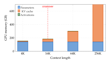
Modern large language models are, at their core, memory systems. A model with 70 billion parameters encodes a vast compressed representation of human knowledge in its weights, yet the act of using that knowledge, generating a single new token, requires attending to every token that has come before. The key–value (KV) cache that stores past attention states can, for long contexts, consume more GPU memory than the model weights themselves. This chapter studies the mathematics of memory in large language models: from the hardware memory hierarchy that constrains every forward pass, through algorithmic techniques that tame the KV cache, to architectural innovations that equip Transformers with external, retrieval-based, and hash-indexed memory systems.

The fundamental tension is between what a model knows (encoded in its parameters) and what it can access (limited by the context window and available hardware memory). Scaling laws tell us that larger models and longer contexts improve capability, but both axes of scaling run headlong into memory walls: the former into GPU VRAM limits, the latter into the quadratic (training) and linear (inference) growth of attention memory.

Key Idea.

Memory Heterogeneity Thesis. Different types of knowledge require different memory mechanisms, each with its own access pattern, latency, and capacity. Parametric memory (model weights) stores slow-changing world knowledge; contextual memory (the KV cache) stores the evolving state of the current conversation; external memory (retrieval corpora, memory tables) provides unbounded storage at the cost of higher access latency. Effective LLM systems must manage all three simultaneously.

[colback=keyamberbg, colframe=keyamber, title=Central Question] How can we organise memory, across hardware levels and architectural levels, to enable LLMs to reason over arbitrarily long contexts without proportional cost growth?

Historical Note.

The idea that computation requires a hierarchy of memory dates to von Neumann's 1945 “First Draft of a Report on the EDVAC,” which described a stored-program architecture with fast registers, intermediate storage, and slow external memory. Eighty years later, the same hierarchy (registers, SRAM, HBM, DRAM, SSD) governs the design of every large language model deployment.

Neural memory systems emerged with Hopfield networks (1982) and were revitalised by Graves et al.'s Neural Turing Machine [1] and Weston et al.'s Memory Networks [2] in 2014–2015. These architectures demonstrated that neural networks could learn to read from and write to external memory banks via differentiable addressing. The modern KV cache crisis, where a single long-context inference can require hundreds of gigabytes of memory, has brought memory management back to the centre of LLM research.

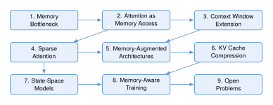
Before diving into the technical development, we provide a roadmap of the chapter. Attention as Memory Access reframes the attention mechanism (Definition 12) as a differentiable memory access operation and quantifies the KV cache growth problem (Definition 16). Extending the Context Window studies methods for extending the effective context window via position-encoding manipulation. Sparse and Structured Attention Patterns introduces sparse and structured attention patterns that reduce the memory footprint. Memory-Augmented Architectures covers memory-augmented architectures, from Neural Turing Machines through the Engram architecture to retrieval-augmented generation. Hierarchical Memory Architectures builds these into hierarchical memory systems, State-Space Models and Recurrent Memory replaces the cache with a fixed recurrent state, and Connections and Synthesis draws the whole landscape onto a single capacity-latency frontier.

Chapter roadmap. Arrows indicate conceptual dependencies.

We assume familiarity with the Transformer architecture as developed in The Transformer, including scaled dot-product attention (Definition 12), multi-head attention (Definition 13), and rotary position embeddings (Definition 15). Readers seeking background on recurrence-based sequence models may consult Recurrent Foundations for Iterative Computation.

Attention as Memory Access

The attention mechanism, when viewed through the lens of memory systems, is a differentiable associative memory. In this section we make that analogy precise, quantify the memory cost of the KV cache, and identify the bandwidth bottleneck that dominates autoregressive generation.

Self-Attention as Differentiable Memory Read

Consider a standard self-attention layer (Definition 12). At generation step $t$ , the model has produced tokens $x_{1}, \dots, x_{t}$ and the KV cache (Definition 16) stores key and value vectors for all prior positions: (KV Cache Matrices) $\begin{matrix} K_{t} & = [\begin{matrix} 𝒌_{1}^{⊤} \\ 𝒌_{2}^{⊤} \\ ⋮ \\ 𝒌_{t}^{⊤} \end{matrix}] \in ℝ^{t \times d_{k}}, & V_{t} & = [\begin{matrix} 𝒗_{1}^{⊤} \\ 𝒗_{2}^{⊤} \\ ⋮ \\ 𝒗_{t}^{⊤} \end{matrix}] \in ℝ^{t \times d_{v}} . \end{matrix}$ To generate token $t + 1$ , the model computes a query $𝒒_{t + 1} \in ℝ^{d_{k}}$ from the embedding of $x_{t}$ and reads from the cache: (ATTN AS READ) $\begin{matrix} {output}_{t + 1} = \underset{read weights 𝒘 \in ℝ^{1 \times t}}{\underset{⏟}{softmax (\frac{𝒒_{t + 1}^{⊤} K_{t}^{⊤}}{\sqrt{d_{k}}})}} V_{t} . \end{matrix}$

Remark 1 (Attention as Associative Memory).

(ATTN AS READ) is precisely a content-based memory read operation:

Memory bank: $V_{t}$ stores $t$ value vectors (the “data” to be retrieved).
Address keys: $K_{t}$ stores $t$ key vectors (the “index” for lookup).
Query: $𝒒_{t + 1}$ specifies what information is needed.
Read head: The softmax-weighted combination is a soft lookup: every memory slot contributes, weighted by relevance.

This is analogous to the content-based addressing in Neural Turing Machines [1], but with the memory bank growing by one entry per time step.

Multi-head attention (Definition 13) can be viewed as $h$ parallel read heads, each with its own query–key subspace. Grouped query attention (Definition 17) shares key–value banks across groups of read heads, reducing the memory bank size at the cost of some independence between heads.

Insight.

The KV cache is not merely an implementation optimisation; it is the model's working memory. Every token the model has seen is stored as a (key, value) pair, and every new token accesses that memory via a soft content-addressed read. The “context window” is simply the size of this working memory.

The KV Cache Growth Problem

We now quantify the memory cost precisely.

Definition 1 (Memory Complexity of Attention).

For a Transformer with $L$ layers, $h$ attention heads per layer, head dimension $d_{k}$ , and sequence length $n$ , the KV cache requires (KV Memory) $\begin{matrix} M_{KV} (n) = 2 L h d_{k} n elements \end{matrix}$ stored in the model's working precision. In half-precision (fp16 or bf16), this corresponds to $2 L h d_{k} n \times 2$ bytes $= 4 L h d_{k} n$ bytes.

The factor of 2 in (KV Memory) accounts for both the key and value matrices. For reference, see the concrete memory budgets computed in Remark 11.

Example 1 (KV Cache of a 70B Model).

Consider a model with $L = 80$ layers, $h = 64$ heads, $d_{k} = 128$ , and sequence length $n = 128,000$ tokens. In fp16: $\begin{matrix} M_{KV} & = 4 \times 80 \times 64 \times 128 \times 128,000 bytes \\ = 4 \times 80 \times 64 \times 128 \times 128,000 \\ = 335,544,320,000 bytes = 335.5 GB = 312.5 GiB . \end{matrix}$ The model weights themselves (70B parameters in fp16) occupy $70 \times 10^{9} \times 2 = 140$ ;GB. At 128K context, the KV cache is more than twice the size of the model weights (a ratio of $2.40$ ). Both figures here are decimal: $1 GB = 10^{9}$ bytes. The binary value $312.5$ ;GiB is the same quantity, and mixing the two units is the most common way to lose a factor of $1.074$ in this arithmetic.

Proposition 1 (Compute–Memory Crossover).

During autoregressive generation, producing a single new token at position $n + 1$ requires:

KV cache read: $Θ (L h d_{k} n)$ bytes of memory access (reading all keys and values across all layers).
Attention computation: $Θ (L h d_{k} n)$ FLOPs (computing the dot products $𝒒_{n + 1}^{⊤} 𝒌_{j}$ for all $j$ and the weighted sum over values).

Define the arithmetic intensity $ℐ = FLOPs / bytes$ . For the attention operation during decoding, $ℐ \approx 1$ (one FLOP per byte read). The system is compute-bound when $ℐ > F_{peak} / {BW}_{HBM}$ and memory-bound otherwise. Since modern accelerators have $F_{peak} / {BW}_{HBM} ≫ 1$ (for an H100 SXM in fp16 or bf16, $989.4 TFLOP/s / 3.35 TB/s \approx 295$ FLOP per byte, and $\approx 148$ in TF32), the attention decoding step is almost always memory-bound.

Proof.

Each attention head in each layer requires reading $n$ key vectors of dimension $d_{k}$ (totalling $n \cdot d_{k}$ values in fp16, i.e., $2 n d_{k}$ bytes) and $n$ value vectors ( $2 n d_{k}$ bytes), for a total of $4 n d_{k}$ bytes per head per layer. Across $L$ layers and $h$ heads: $4 L h d_{k} n$ bytes.

The corresponding computation is $n$ dot products of dimension $d_{k}$ (costing $2 n d_{k}$ FLOPs per head, using the convention that a multiply-add is 2 FLOPs) plus a further $2 n d_{k}$ FLOPs for the weighted sum, which is also $n d_{k}$ multiply-adds. That gives $4 n d_{k}$ FLOPs per head per layer and $4 L h d_{k} n$ FLOPs in total, matching the byte count exactly.

The arithmetic intensity is therefore $ℐ = \frac{4 L h d_{k} n FLOPs}{4 L h d_{k} n bytes} = 1 FLOP per byte .$ Since $F_{peak} / {BW}_{HBM} ≫ 1$ for all current accelerators, we have $ℐ < F_{peak} / {BW}_{HBM}$ , and the operation is memory-bandwidth–bound.

∎

The Memory Bandwidth Wall

Definition 2 (Memory Bandwidth Bottleneck).

During autoregressive generation, each new token requires reading the entire KV cache from HBM\@. The maximum token generation throughput is therefore bounded by (Bandwidth Bound) $\begin{matrix} Tokens/second \leq \frac{{BW}_{HBM}}{M_{KV} (n) + M_{params}}, \end{matrix}$ where $M_{params}$ is the memory footprint of model parameters (which must also be read for the FFN layers).

Example 2 (Throughput on an H100).

An NVIDIA H100 SXM provides ${BW}_{HBM} = 3.35$ TB/s. For the 70B model at 128K context from Example 1: $Tokens/s \leq \frac{3.35 \times 10^{12}}{(335.5 + 140) \times 10^{9}} = \frac{3350}{475.5} \approx 7.04 tokens/s .$ This is per sequence. Batching multiple sequences helps amortise the parameter reads but exacerbates the KV cache memory pressure.

The memory wall for a 70B-parameter model (fp16). Model parameters are constant at 140;GB. The KV cache grows linearly with context length at

2.62

;MB per token, and passes the parameter memory at

140 \times 10^{9} / 2,621,440 = 53,406

tokens, between the 16K and 64K bars. Activation memory (for a single-token decode step) is comparatively negligible.

Caution.

The quadratic cost of attention ( $O (n^{2})$ in FLOPs and memory) is often cited as the primary bottleneck. However, during autoregressive generation, which is the dominant workload for deployed LLMs, each step computes attention for a single new query against $n$ cached keys, costing $O (n)$ FLOPs but requiring $O (n)$ memory reads. The linear KV cache growth and the resulting bandwidth bottleneck are the more pressing constraints in practice. Flash Attention (Algorithm 3, Proposition 2) addresses the IO cost during training (prefill), but the decode-time bandwidth wall persists.

The rest of this chapter is devoted to techniques for pushing past this memory wall: extending the context window without proportional memory growth (Extending the Context Window), reducing the number of positions that attend to each other (Sparse and Structured Attention Patterns), augmenting the Transformer with external memory (Memory-Augmented Architectures), organising those stores into a hierarchy (Hierarchical Memory Architectures), and replacing the cache altogether with a fixed-size recurrent state (State-Space Models and Recurrent Memory).

Extending the Context Window

A model trained on sequences of length $L_{train}$ must, at deployment, often handle sequences of length $L_{test} ≫ L_{train}$ . Naïve extrapolation fails: the model encounters position encodings outside its training distribution. This section presents three progressively more sophisticated methods for extending the context window, all of which manipulate the frequency schedule of rotary position embeddings (Definition 15).

Position Interpolation

Definition 3 (Position Interpolation).

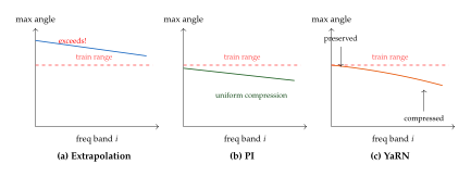
Let a model be trained with maximum sequence length $L_{train}$ using RoPE (Definition 15). Position Interpolation (PI) [3] rescales position indices during inference to fit within the training range: (PI Rescale) $\begin{matrix} m ⟼ m \cdot \frac{L_{train}}{L_{test}}, m = 0, 1, \dots, L_{test} - 1. \end{matrix}$ The rescaled positions $m^{'} = m \cdot L_{train} / L_{test}$ are no longer integers, but the RoPE rotation $R_{θ} (m^{'})$ is well defined for all $m^{'} \in ℝ$ .

The intuition is simple: instead of extrapolating to unseen positions $m > L_{train}$ , we interpolate between the positions seen during training. The price is reduced positional resolution: positions that were distinguishable at training time may become aliased.

Proposition 2 (PI Angle Bound).

Under Position Interpolation, the maximum rotation angle for RoPE frequency band $i$ over the admissible positions $m \in {0, \dots, L_{test} - 1}$ is $\begin{matrix} \max_{m \leq L_{test} - 1} | m^{'} \cdot θ_{i} | = \frac{L_{test} - 1}{L_{test}} \cdot L_{train} \cdot θ_{i} < L_{train} \cdot θ_{i}, \end{matrix}$ so every angle stays strictly inside the range seen during training.

Proof.

By definition of PI ((PI Rescale)), $m^{'} = m \cdot L_{train} / L_{test}$ . The rotation angle for frequency band $i$ is $m^{'} θ_{i}$ . The maximum over $m \in {0, \dots, L_{test} - 1}$ is achieved at $m = L_{test} - 1$ : $m^{'} θ_{i} = \frac{(L_{test} - 1) \cdot L_{train}}{L_{test}} \cdot θ_{i} < L_{train} \cdot θ_{i} .$ Since during training the maximum angle was $(L_{train} - 1) \cdot θ_{i} \leq L_{train} \cdot θ_{i}$ , all interpolated angles lie within the training range.

∎

Remark 2.

PI preserves the relative-position property of RoPE (Proposition 1): the dot product between the query at position $m_{1}$ and the key at position $m_{2}$ depends only on $m_{1} - m_{2}$ (rescaled). However, the rescaled relative distances become $Δ^{'} = (m_{1} - m_{2}) \cdot L_{train} / L_{test}$ , which compresses the position spectrum and may degrade local position discrimination.

NTK-Aware Scaling

Position Interpolation applies the same compression ratio to all frequency bands. But high-frequency bands encode local position information (nearby tokens), while low-frequency bands encode global position information (distant tokens). Compressing high frequencies degrades local discrimination unnecessarily.

Definition 4 (NTK-Aware Scaling).

Instead of uniformly interpolating all frequencies, NTK-Aware Scaling adjusts the RoPE base frequency: (NTK BASE) $\begin{matrix} θ_{base}^{'} = θ_{base} \cdot α^{d / (d - 2)}, \end{matrix}$ where $α = L_{test} / L_{train}$ is the extension ratio and $d$ is the head dimension. The individual frequency bands become $\begin{matrix} θ_{i}^{'} = \frac{1}{{(θ_{base}^{'})}^{2 i / d}} = \frac{1}{θ_{base}^{2 i / d} \cdot α^{2 i / (d - 2)}}, i = 0, 1, \dots, \frac{d}{2} - 1. \end{matrix}$

The key property of NTK-Aware Scaling is that the compression factor varies across frequency bands:

For $i = 0$ (highest frequency): the scaling factor is $α^{0} = 1$ , meaning no compression at all.
For $i = d / 2 - 1$ (lowest frequency): the scaling factor approaches $α$ , giving maximum compression, similar to PI\@.

This preserves local positional precision while extending global reach.

Remark 3.

The name “NTK-Aware” comes from an analogy with neural tangent kernel (NTK) theory: the base-frequency adjustment ensures that the effective learning rate for each frequency band remains balanced, in the same way that NTK parameterisation balances gradient norms across layers.

YaRN: Yet Another RoPE ExtensioN

Definition 5 (YaRN).

YaRN [4] combines NTK-aware scaling with an attention temperature correction. The modified attention computation is (YARN ATTN) $\begin{matrix} {Attention}_{YaRN} (Q, K, V) = softmax (\frac{1}{t} \cdot \frac{Q K^{⊤}}{\sqrt{d_{k}}}) V, \end{matrix}$ where the temperature $t$ is given by the empirical fit (YARN TEMP) $\begin{matrix} \sqrt{1 / t} = 0.1 \ln (α) + 1, α = \frac{L_{test}}{L_{train}}, \end{matrix}$ so that the logits are multiplied by $1 / t = (0.1 \ln α + 1)^{2}$ . Note the square: the quantity $0.1 \ln α + 1$ is $\sqrt{1 / t}$ , not the logit multiplier itself. The coefficient $0.1$ is fitted empirically to the LLaMA family in the original work rather than derived. The temperature compensates for the entropy increase caused by position interpolation: when positions are compressed, the attention logits decrease in magnitude, leading to a more uniform (higher entropy) attention distribution. The factor $t > 1$ sharpens the distribution to restore the original attention pattern.

Remark 4.

YaRN additionally partitions the frequency bands into three groups:

No interpolation (highest frequencies, $i < i_{\min}$ ): leave unchanged.
NTK interpolation (middle frequencies, $i_{\min} \leq i \leq i_{\max}$ ): apply the NTK-aware scaling from Definition 4.
Linear interpolation (lowest frequencies, $i > i_{\max}$ ): apply PI-style uniform compression.

The boundaries $i_{\min}$ and $i_{\max}$ are determined by a wavelength threshold relative to $L_{train}$ .

Maximum rotation angles across RoPE frequency bands for three context extension strategies. (a) Naïve extrapolation pushes high-frequency bands beyond the training range. (b) Position Interpolation (PI) compresses all bands uniformly. (c) YaRN preserves high-frequency (local) bands while compressing low-frequency (global) bands, and applies a temperature correction to the attention logits.

Insight.

All context extension methods manipulate the same mathematical object, the RoPE frequency schedule ${θ_{i}}_{i = 0}^{d / 2 - 1}$ , but with different trade-offs between local precision and global reach. PI compresses uniformly (simple but lossy at short range), NTK-Aware scaling compresses adaptively (preserving local info), and YaRN adds temperature correction to counteract entropy distortion. The progression illustrates a general principle: when extrapolating a learned representation, it is better to preserve the components the model relies on most (high-frequency, local structure) and compress those it is more robust to (low-frequency, global structure).

Example 3 (LLaMA-2 Context Extension).

Consider extending LLaMA-2 from $L_{train} = 4,096$ to $L_{test} = 131,072$ tokens. The extension ratio is $α = 131,072 / 4,096 = 32$ . LLaMA-2 uses $θ_{base} = 10,000$ and head dimension $d = 128$ .

PI scaling. All position indices are scaled by $1 / 32$ . Position $m = 131,071$ maps to $m^{'} = 4,095.97$ , within the training range. The minimum distinguishable position gap is $Δ m^{'} = 1 / 32 \approx 0.03$ positions.

NTK base frequency. From (NTK BASE): $θ_{base}^{'} = 10,000 \times 32^{128 / 126} = 10,000 \times 32^{1.0159} \approx 10,000 \times 33.81 = 338,097.$ The lowest-frequency band ( $i = 63$ ) sees a compression factor close to $32$ , while the highest-frequency band ( $i = 0$ ) is virtually unchanged.

YaRN temperature. From (YARN TEMP): $\sqrt{1 / t} = 0.1 \times \ln (32) + 1 = 0.1 \times 3.4657 + 1 = 1.3466, \frac{1}{t} = {1.3466}^{2} = 1.8133.$ All attention logits are multiplied by $1.8133$ , sharpening the softmax distribution to compensate for the reduced magnitude of interpolated position encodings. Applying $1.3466$ instead would correct only about half the entropy increase, since that quantity is $\sqrt{1 / t}$ .

Exercise 1.

Show that under Position Interpolation with extension ratio $α$ , the minimum relative position difference that produces a distinct attention pattern is $α$ times larger than during training. Specifically, if two positions $m_{1}, m_{2}$ with $| m_{1} - m_{2} | = 1$ were distinguishable during training, then under PI the minimum distinguishable gap is $| m_{1} - m_{2} | = α$ . Hint: Consider the dot product $𝒒_{m_{1}}^{⊤} 𝒌_{m_{2}}$ as a function of $m_{1} - m_{2}$ and compare the rescaled version.

Exercise 2.

Derive the NTK-aware scaling formula by requiring that:

The highest-frequency band ( $i = 0$ ) is unmodified: $θ_{0}^{'} = θ_{0}$ .
The lowest-frequency band ( $i = d / 2 - 1$ ) is compressed by factor $α$ : $θ_{d / 2 - 1}^{'} = θ_{d / 2 - 1} / α$ .
The intermediate bands interpolate geometrically between these extremes.

Show that these constraints uniquely determine $θ_{base}^{'} = θ_{base} \cdot α^{d / (d - 2)}$ .

Sparse and Structured Attention Patterns

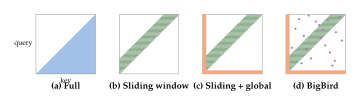
Full attention requires every token to attend to every other token, yielding $O (n^{2})$ memory and computation during training (and $O (n)$ KV cache reads per step during generation). Sparse attention restricts the set of (query, key) pairs that interact, reducing cost while preserving the ability to propagate information across the full sequence.

Formalising Sparse Attention

Definition 6 (Sparse Attention Pattern).

An attention pattern is a relation $P \subseteq {1, \dots, n}^{2}$ specifying which (query, key) pairs interact. For each query position $i$ , define the receptive field $P_{i} = {j : (i, j) \in P}$ . The sparse attention under pattern $P$ is (Sparse ATTN) $\begin{matrix} {Attention}_{P} {(Q, K, V)}_{i} = \sum_{j \in P_{i}} {softmax}_{j^{'} \in P_{i}} {(\frac{𝒒_{i}^{⊤} 𝒌_{j^{'}}}{\sqrt{d_{k}}})}_{j} 𝒗_{j}, \end{matrix}$ where the softmax is restricted to the receptive field $P_{i}$ . The per-token memory and computation cost is $O (| P_{i} |)$ instead of $O (n)$ .

Remark 5.

Full (dense) attention corresponds to $P_{full} = {(i, j) : 1 \leq j \leq i}$ (causal) or $P_{full} = {1, \dots, n}^{2}$ (bidirectional). Any sparse pattern $P \subset P_{full}$ sacrifices some information flow in exchange for efficiency.

The Sliding Window

Definition 7 (Sliding Window Attention).

The sliding window pattern with window size $w$ is (Sliding Window) $\begin{matrix} P_{sw} = {(i, j) : 0 \leq i - j \leq w} . \end{matrix}$ Each token attends to at most $w + 1$ positions (itself and the $w$ preceding tokens). The memory cost of the KV cache is reduced from $O (n)$ to $O (w)$ per layer, since keys and values outside the window can be evicted.

Proposition 3 (Sliding Window Information Propagation).

In a Transformer with $L$ layers of sliding window attention with window size $w$ , information from position $j$ can reach position $i$ (with $i > j$ ) if and only if $i - j \leq L \cdot w$ . The effective receptive field is $L \cdot w$ tokens.

Proof.

In a single layer, position $i$ receives information from positions ${i - w, \dots, i}$ . After two layers, position $i$ receives information from positions up to $i - 2 w$ (since each position in its first-layer receptive field itself has a window of size $w$ ). By induction, after $L$ layers, the receptive field extends back to position $\max (1, i - L w)$ .

∎

Example 4 (Mistral 7B).

Mistral 7B uses sliding window attention with $w = 4,096$ and $L = 32$ layers. The effective receptive field is $32 \times 4,096 = 131,072$ tokens, enabling the model to process very long contexts while keeping the per-layer KV cache at $O (4,096)$ instead of $O (n)$ .

Global Tokens and the BigBird Pattern

A pure sliding window cannot propagate information globally in a single layer. Adding a small set of global tokens, positions that attend to (and are attended by) all other positions, restores global connectivity.

Definition 8 (BigBird Attention Pattern).

The BigBird pattern [5] is the union of three sub-patterns: (Bigbird) $\begin{matrix} P_{BigBird} = P_{sw}^{bi} \cup P_{global} \cup P_{random}, \end{matrix}$ where:

$P_{sw}^{bi} = {(i, j) : | i - j | \leq w}$ is a sliding window of size $w$ . BigBird is presented here in the bidirectional (encoder) setting, so this window spans $2 w + 1$ positions, unlike the causal $P_{sw}$ of Definition 7, which spans $w + 1$ .
$P_{global} = {(i, j) : i \in G or j \in G}$ for a set $G$ of global token positions. Every position attends to global tokens and vice versa.
$P_{random} \subseteq {1, \dots, n}^{2}$ contains $r$ randomly chosen pairs per query position, providing stochastic long-range connections.

The per-token memory cost is $O (w + | G | + r)$ .

The Longformer [22] uses a similar pattern (sliding window + global tokens, without the random component).

Theorem 1 (Information Propagation in BigBird).

For the BigBird attention pattern with at least $| G | \geq 1$ global token and window size $w \geq 1$ , the attention graph has diameter at most $2$ : any two positions $i, j \in {1, \dots, n}$ are joined by a path of length at most 2, so two layers suffice for any $w \geq 1$ . Without global tokens, the sliding window alone gives a diameter of $⌈ \frac{n}{w} ⌉$ , and covering a separation of $n$ in two layers would require $2 w \geq n$ .

Proof.

We construct an explicit path in the attention graph.

Case 1: $j \in G$ or $i \in G$ . Then $(i, j) \in P_{global}$ directly, giving a path of length 1.

Case 2: Neither $i$ nor $j$ is a global token. Choose any $g \in G$ . The path is $j \to g \to i$ :

$j \to g$ : Since $g$ is a global token, $(g, j) \in P_{global}$ , so $g$ attends to $j$ .
$g \to i$ : Since $g$ is global, $(i, g) \in P_{global}$ , so $i$ attends to $g$ .

This gives a path of length 2 via the global token.

Cases 1 and 2 are exhaustive, and each yields a path of length at most 2, so the diameter is at most 2 whenever $| G | \geq 1$ .

If the global tokens are removed, or if their capacity is exhausted so that they cannot be relied on, the only remaining edges are the window edges. A position can then move at most $w$ places per hop, so crossing a separation of $| i - j |$ takes $⌈ | i - j | / w ⌉$ hops and the window-only diameter is $⌈ n / w ⌉$ . In particular two layers reach only $2 w$ , so two-layer coverage of the whole sequence needs $2 w \geq n$ .

∎

Remark 6.

It is worth separating the two bounds, because they differ by a large factor in practice. At $n = 4096$ and $w = 128$ the window-only diameter is $32$ , while a single global token brings the diameter to $2$ . The lesson is that connectivity in these patterns is bought by the hubs, not by the window; the window buys locality.

Remark 7.

Zaheer et al. [5] proved a stronger result: BigBird with random attention is a universal approximator of sequence-to-sequence functions, matching the expressiveness of full attention under mild assumptions on the number of global and random connections.

Ring Attention for Distributed Long Context

Sparse attention reduces per-device memory, but for very long sequences even the reduced KV cache may not fit on a single device. Ring Attention [23] distributes the full sequence across multiple devices while computing exact (dense) attention.

Proposition 4 (Ring Attention).

Partition a sequence of length $n$ evenly across $P$ devices, so device $p$ holds tokens ${p \cdot n / P + 1, \dots, (p + 1) \cdot n / P}$ with their query, key, and value projections. In each of $P$ rounds:

Each device computes local attention between its queries and the currently-held keys/values (a block of $n / P$ tokens).
Keys and values are passed to the next device in a ring topology.

After $P$ rounds, each device has computed attention against all $n$ keys. The per-device memory is $O (n / P \cdot d_{k})$ for keys/values, and the total communication per device per head per layer is (RING COMM) $\begin{matrix} Communication = (P - 1) \times \frac{2 n d_{k}}{P} \times 2 bytes = \frac{4 (P - 1)}{P} n d_{k} bytes < 4 n d_{k} bytes = O (n d_{k}) . \end{matrix}$ The factor $2$ accounts for both keys and values.

Proof.

Each device sends its local KV block (of size $n / P$ tokens, each with $d_{k}$ -dimensional key and value, totalling $2 \cdot (n / P) \cdot d_{k}$ elements) to the next device. This happens $P - 1$ times (after $P$ rounds, the original block returns and no further send is needed). Total elements sent per device: $(P - 1) \times \frac{2 n d_{k}}{P} < 2 n d_{k} .$ In fp16, this is at most $4 n d_{k}$ bytes per device per head per layer, confirming $O (n d_{k})$ communication.

Computation overlaps with communication: while device $p$ sends its KV block to device $p + 1$ , it computes attention on the block it just received. With sufficient bandwidth, the communication is fully hidden, and the wall-clock time is dominated by the $P$ sequential attention computations of size ${(n / P)}^{2}$ .

∎

Remark 8.

Ring Attention is exact: it computes the same result as full dense attention. It is purely a systems-level optimisation that distributes the memory burden. Combining Ring Attention with sparse patterns (e.g., using a sliding window within each block and global tokens across blocks) further reduces both communication and computation.

Sparse attention patterns visualised as binary matrices (query positions on the vertical axis, key positions on the horizontal axis; filled entries indicate allowed attention pairs). (a) Full causal attention. (b) Sliding window: a diagonal band of width

w

. (c) Sliding window plus global tokens (first few positions attend to and are attended by all others). (d) BigBird: sliding window, global tokens, and random connections (purple dots).

Key Idea.

Sparse attention trades global information reach for efficiency. The fundamental design question is: which tokens truly need to attend to which? Global tokens ensure connectivity; sliding windows preserve local structure; random connections provide stochastic shortcuts. The optimal pattern depends on the task: local patterns suffice for language modelling where nearby context is most predictive, while tasks requiring long-range reasoning (e.g., document QA, code understanding) may require denser global connectivity.

Exercise 3.

For the BigBird pattern with $g = | G |$ global tokens, window size $w$ , and $r$ random connections per query:

Show that the per-token memory cost is $O (w + g + r)$ .
Show that the total attention FLOPs for a sequence of length $n$ is $O (n (w + g + r) \cdot d_{k})$ .
Determine the condition on $w$ , $g$ , and $r$ under which the BigBird pattern achieves sub-quadratic total cost in $n$ .

Exercise 4.

In Ring Attention with $P$ devices, the computation of each local attention block takes time $T_{comp} = O ({(n / P)}^{2} d_{k})$ and the communication of each KV block takes time $T_{comm} = O (n \cdot d_{k} / (P \cdot B))$ , where $B$ is the inter-device bandwidth. Show that the communication is fully hidden (i.e., $T_{comm} \leq T_{comp}$ ) when $n / P \geq B^{- 1}$ , i.e., when each device holds sufficiently many tokens.

Memory-Augmented Architectures

The KV cache is the Transformer's working memory: it stores contextual information that persists within a single forward pass. But it is ephemeral (cleared between sequences), bounded (limited by GPU memory), and expensive (every entry is read at every step). Memory-augmented architectures add a persistent, structured external memory that the model can read from (and sometimes write to) using learned addressing mechanisms. This section traces the evolution from Neural Turing Machines through modern architectures like Engram and retrieval-augmented generation.

Neural Turing Machines and Differentiable Neural Computers

Definition 9 (External Memory).

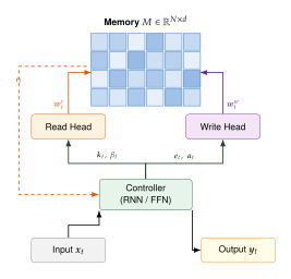
An external memory is a matrix $M \in ℝ^{N \times d}$ , where $N$ is the number of memory slots and $d$ is the slot dimension. A controller network interacts with the memory through read and write heads.

Read operation. A read head produces a weight vector $𝒘_{t}^{r} \in Δ^{N - 1}$ (a probability distribution over slots) and returns (Memory READ) $\begin{matrix} 𝒓_{t} = \sum_{i = 1}^{N} w_{t}^{r} (i) \cdot M_{t} (i), \end{matrix}$ where $M_{t} (i) \in ℝ^{d}$ is the $i$ -th row of the memory matrix at time $t$ .

Content-based addressing. The read weights can be computed via content-based addressing: (Content Addressing) $\begin{matrix} w_{t}^{c} (i) = \frac{\exp (β_{t} \cdot \cos (𝒌_{t}, M_{t} (i)))}{\sum_{j = 1}^{N} \exp (β_{t} \cdot \cos (𝒌_{t}, M_{t} (j)))}, \end{matrix}$ where $𝒌_{t} \in ℝ^{d}$ is a query key emitted by the controller, $β_{t} > 0$ is a sharpness parameter, and $\cos (\cdot, \cdot)$ denotes cosine similarity.

Write operation. A write head produces an erase vector $𝒆_{t} \in {[0,1]}^{d}$ and an add vector $𝒂_{t} \in ℝ^{d}$ : (Memory Write) $\begin{matrix} M_{t} (i) = M_{t - 1} (i) \cdot (𝟏 - w_{t}^{w} (i) 𝒆_{t}) + w_{t}^{w} (i) 𝒂_{t}, \end{matrix}$ where $w_{t}^{w}$ is the write weight distribution.

Historical Note.

Graves et al. [1] introduced the Neural Turing Machine (NTM), which augmented a recurrent neural network controller with a differentiable external memory and read/write heads using both content-based and location-based addressing. The Differentiable Neural Computer (DNC) [6] improved upon the NTM with dynamic memory allocation, temporal link matrices for tracking the order of writes, and a usage-based free mechanism.

Concurrently, Weston et al. [2] introduced Memory Networks with a simpler architecture: a large memory bank of (key, value) pairs addressed purely by content, without a write mechanism. End-to-end Memory Networks made the addressing differentiable, enabling training with backpropagation.

These architectures demonstrated that neural networks could learn to use external memory for algorithmic tasks (copying, sorting, graph traversal), but they faced challenges at scale: the fixed memory size $N$ limited capacity, content-based addressing became noisy for large $N$ , and the recurrent controller made training slow.

Remark 9.

Comparing (Content Addressing) with standard attention ((ATTN AS READ)) reveals a striking parallel:

	NTM Read	Attention
Memory bank	$M_{t} \in ℝ^{N \times d}$	$V_{t} \in ℝ^{n \times d_{v}}$
Address keys	$M_{t}$ (reused)	$K_{t} \in ℝ^{n \times d_{k}}$
Query	$𝒌_{t}$ (controller)	$𝒒_{t}$ (projected)
Similarity	cosine	dot product / $\sqrt{d_{k}}$
Sharpness	$β_{t}$ (learned)	$1 / \sqrt{d_{k}}$ (fixed)

Attention can be viewed as a streamlined NTM read with the address keys decoupled from the values and the sharpness fixed.

Neural Turing Machine architecture. The controller emits query keys and sharpness parameters for the read head, and erase/add vectors for the write head. The read head performs content-based addressing ((Content Addressing)) to retrieve a weighted sum from the memory matrix. The write head updates memory via (Memory Write). The read vector

𝒓_{t}

is fed back to the controller for the next time step.

N-gram Hash Memory: The Engram Architecture

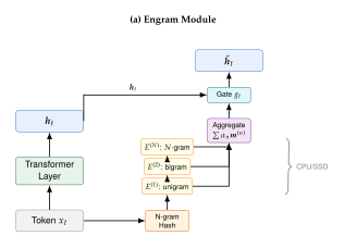
While NTMs use a small, fully differentiable memory, modern LLMs need memory systems that can scale to billions of entries. The Engram architecture [24] takes a radically different approach: instead of learning the addressing mechanism end-to-end, it uses a fixed hash function to index into a massive lookup table, trading addressing flexibility for scalability.

Definition 10 (N-gram Hash Function).

For a sequence of token IDs $x_{1}, x_{2}, \dots$ , the $n$ -gram hash at position $t$ is computed via a polynomial rolling hash: (Ngram HASH) $\begin{matrix} h_{n} (x_{t - n + 1 : t}) = (\sum_{i = 0}^{n - 1} x_{t - n + 1 + i} \cdot p^{i}) mod T, \end{matrix}$ where $p$ is a prime number and $T$ is the hash table size. This maps each $n$ -gram of token IDs to an integer in ${0, 1, \dots, T - 1}$ .

Remark 10.

The polynomial rolling hash spreads $V^{n}$ possible $n$ -grams over $T$ buckets, giving an expected bucket load of $V^{n} / T$ entries per bucket, while the probability that two specified distinct $n$ -grams land in the same bucket is $1 / T$ . The two quantities answer different questions and only the second is a probability: at $V = 32,000$ , $T = 10^{7}$ and $n = 2$ the load is $102.4$ per bucket while the pairwise probability is $10^{- 7}$ . For $T ≫ V^{n}$ the buckets are mostly empty and collisions are rare. For large $n$ , collisions are inevitable and can be viewed as a form of implicit dimensionality reduction: similar $n$ -grams may share a memory slot, forcing the memory to store generalisable patterns rather than memorising every sequence.

Definition 11 (Engram Module).

Given a token sequence $x_{1}, \dots, x_{t}$ and the hidden state $𝒉_{t} \in ℝ^{d}$ from a Transformer layer, the Engram module computes:

N-gram hashing: For each $n$ -gram order $n \in {1, 2, \dots, N_{\max}}$ , compute the hash $h_{n} = h_{n} (x_{t - n + 1 : t})$ using (Ngram HASH), which already reduces modulo $T$ .
Table lookup: Retrieve the memory vector (Engram Lookup) $\begin{matrix} 𝒎_{t}^{(n)} = E^{(n)} [h_{n}] \in ℝ^{d}, \end{matrix}$ where $E^{(n)} \in ℝ^{T \times d}$ is a learnable embedding table for $n$ -gram order $n$ .
Aggregation: Combine across $n$ -gram orders: (Engram Aggregate) $\begin{matrix} 𝒎_{t} = \sum_{n = 1}^{N_{\max}} α_{n} 𝒎_{t}^{(n)}, \end{matrix}$ where $𝜶 = (α_{1}, \dots, α_{N_{\max}})$ are learned (and optionally input-dependent) mixing weights.
Gated fusion: Merge the memory vector with the hidden state: (Engram GATE) $\begin{matrix} {\tilde{𝒉}}_{t} = 𝒉_{t} + g_{t} ⊙ 𝒎_{t}, g_{t} = σ (W_{g} 𝒉_{t} + 𝒃_{g}), \end{matrix}$ where $g_{t} \in {(0,1)}^{d}$ is a learned gate, $W_{g} \in ℝ^{d \times d}$ , $𝒃_{g} \in ℝ^{d}$ , and $σ$ is the sigmoid function.

The gate $g_{t}$ allows the model to dynamically control how much memory influence each hidden dimension receives. When $g_{t} \approx 0$ , the Engram module is effectively bypassed, recovering standard Transformer behaviour.

Proposition 5 (Engram Complexity).

The Engram module has the following complexity properties:

Time: $O (N_{\max} d + d^{2})$ per position, independent of context length $n$ and table size $T$ . The $d^{2}$ gating term dominates at realistic sizes ( $d = 4096$ , $N_{\max} = 3$ ).
Memory (parameters): $N_{\max} \cdot T \cdot d$ for the embedding tables, plus $O (d^{2})$ for the gating parameters.
Offloadability: The embedding tables $E^{(n)}$ can be stored on CPU DRAM or SSD\@. Each forward pass requires fetching only $N_{\max}$ vectors of dimension $d$ (one per $n$ -gram order), with less than 3% latency overhead when prefetching is used.

Proof.

(1) Computing each hash ((Ngram HASH)) takes $O (n)$ operations. Summing over $n = 1, \dots, N_{\max}$ , the total hashing cost is $O (N_{\max}^{2})$ , but since $N_{\max}$ is a small constant (typically $\leq 8$ ), this is $O (1)$ . Each table lookup is $O (1)$ (direct indexing). The aggregation ((Engram Aggregate)) and gating ((Engram GATE)) are $O (N_{\max} d)$ and $O (d^{2})$ respectively. Total per-position cost: $O (N_{\max} d + d^{2})$ , independent of both $n$ and $T$ .

(2) Each of the $N_{\max}$ embedding tables has $T$ rows of dimension $d$ , giving $N_{\max} T d$ parameters.

(3) During inference, only the rows indexed by the current $n$ -gram hashes are accessed. These $N_{\max}$ rows (totalling $N_{\max} d$ elements) can be prefetched from CPU/SSD while the Transformer layers compute, hiding the latency.

∎

Theorem 2 (U-Shaped Scaling Law).

Consider a fixed total parameter budget $C$ , with fraction $α$ allocated to Transformer computation (weights of attention and FFN layers) and fraction $1 - α$ allocated to Engram memory tables. Under Chinchilla-style power-law assumptions, the loss contributions from computation and memory are (LOSS COMP) $\begin{matrix} L_{comp} (α C) & = a \cdot (α C)^{- p}, \\ L_{mem} ((1 - α) C) & = b \cdot ((1 - α) C)^{- q}, \end{matrix}$ with $a, b > 0$ and $p, q > 0$ . The total loss (Total LOSS) $\begin{matrix} L (α) = L_{comp} (α C) + L_{mem} ((1 - α) C) \end{matrix}$ is U-shaped in $α$ with a unique interior minimum $α^{*} \in (0, 1)$ .

Proof.

We show that $L (α)$ is strictly convex on $(0,1)$ with boundary behaviour $L (α) \to \infty$ as $α \to 0^{+}$ or $α \to 1^{-}$ , guaranteeing a unique interior minimum.

Step 1: Boundary behaviour. As $α \to 0^{+}$ , $L_{comp} = a {(α C)}^{- p} \to \infty$ . As $α \to 1^{-}$ , $L_{mem} = b {((1 - α) C)}^{- q} \to \infty$ . Thus $L (α) \to \infty$ at both endpoints.

Step 2: First-order condition. Taking the derivative: (DLdalpha) $\begin{matrix} \frac{d L}{d α} & = - a p C^{- p} α^{- p - 1} + b q C^{- q} {(1 - α)}^{- q - 1} . \end{matrix}$ Setting $d L / d α = 0$ : (FOC) $\begin{matrix} a p C^{- p} α^{- p - 1} = b q C^{- q} {(1 - α)}^{- q - 1} . \end{matrix}$ The left-hand side is a strictly decreasing function of $α$ on $(0,1)$ (from $+ \infty$ to a finite positive value), and the right-hand side is a strictly increasing function (from a finite positive value to $+ \infty$ ). By the intermediate value theorem, there is a unique crossing $α^{*} \in (0,1)$ .

Step 3: Second-order condition. $\begin{matrix} \frac{d^{2} L}{d α^{2}} & = a p (p + 1) C^{- p} α^{- p - 2} + b q (q + 1) C^{- q} {(1 - α)}^{- q - 2} > 0 \end{matrix}$ for all $α \in (0,1)$ , confirming strict convexity and that $α^{*}$ is a global minimum.

∎

Remark 11.

When the two exponents coincide, $p = q$ , (FOC) can be solved in closed form: $α^{*} = \frac{1}{1 + {(b / a)}^{1 / (p + 1)}},$ independent of the total budget $C$ , which suggests that in that regime the optimal compute-memory split is a property of the task rather than of the scale. For $p \neq q$ no such elementary solution exists: (FOC) then carries different exponents on $α$ and $1 - α$ , and the root must be found numerically. The difference is not negligible, as Exercise 6 shows: at $a = 1.5$ , $b = 0.8$ , $p = 0.5$ , $q = 0.6$ the true root is $α^{*} = 0.8465$ , so treating the $p = q$ formula as general would misallocate the budget by several per cent.

Insight.

Engram decouples knowledge storage from reasoning computation. Factual knowledge (world facts, code patterns, syntactic $n$ -gram statistics) changes rarely and can live in a massive memory table offloaded to CPU\@. This frees GPU-resident Transformer layers to focus on reasoning and context understanding. The U-shaped scaling law (Theorem 2) formalises the intuition that neither pure computation (all Transformer) nor pure memory (all lookup) is optimal: the best models balance both.

Remark 12 (Connection to Mixture-of-Experts).

Mixture-of-Experts (MoE) [7] provides conditional computation: only a subset of FFN experts are activated per token. Engram provides conditional memory: only the relevant $n$ -gram entries are fetched per token. Together, they span the two axes of model scaling:

	Compute	Memory
Dense	Standard FFN	Full KV cache
Conditional	MoE (sparse experts)	Engram (hash lookup)

A model combining MoE and Engram would have both conditional computation and conditional memory, potentially achieving much better scaling than either approach alone.

(a) Engram module architecture. Token

n

-grams are hashed to index into learnable embedding tables

E^{(1)}, \dots, E^{(N_{\max})}

, which can be offloaded to CPU or SSD\@. Retrieved vectors are aggregated and fused with the Transformer hidden state via a learned gate. (b) U-shaped scaling law (Theorem 2). Allocating all parameters to Transformer computation (

α \to 1

) or all to Engram memory (

α \to 0

) yields high loss. The optimum

α^{*}

balances both.

Exercise 5.

Suppose the vocabulary size is $V = 32,000$ , the hash table size is $T = 10^{7}$ , and we use bigrams ( $n = 2$ ).

How many distinct bigrams are possible?
What is the expected number of bigrams per bucket, and separately, what is the probability that two specified distinct bigrams map to the same hash? Explain why only the second of these is a probability, and check that your first answer exceeds 1.
Argue that collisions can be beneficial: bigrams with similar continuations should ideally share memory entries.

Exercise 6.

For the U-shaped scaling law with $a = 1.5$ , $b = 0.8$ , $p = 0.5$ , $q = 0.6$ , and $C = 10^{10}$ :

Write the first-order condition explicitly.
Solve numerically for $α^{*}$ .
Compute the optimal number of Engram parameters $(1 - α^{*}) C$ and the optimal number of Transformer parameters $α^{*} C$ .

Retrieval-Augmented Generation as External Memory

While NTMs and Engram operate at the vector level (individual memory vectors integrated into the hidden state), retrieval-augmented generation (RAG) operates at the sequence level: entire documents are retrieved and prepended to the context.

Definition 12 (Retrieval-Augmented Generation).

RAG [8] formalises external memory as a two-stage process over a document corpus $𝒟 = {d_{1}, \dots, d_{M}}$ :

Retrieve: Given query $q$ , select the top- $k$ most relevant documents: (RAG Retrieve) $\begin{matrix} 𝒟_{q} = \underset{d \in 𝒟}{top-k} sim (encode (q), encode (d)), \end{matrix}$ where $sim$ is typically the inner product in an embedding space produced by a bi-encoder.
Generate: Produce the output by marginalising over retrieved documents: (RAG Generate) $\begin{matrix} p_{𝜽} (y | q) = \sum_{d \in 𝒟_{q}} p (d | q) \cdot p_{𝜽} (y | q, d), \end{matrix}$ where $p (d | q) \propto \exp (sim (encode (q), encode (d)))$ and $p_{𝜽} (y | q, d)$ is the LLM's output distribution conditioned on the concatenation of the query and the retrieved document.

Remark 13 (RAG vs. Engram: Sequence-Level vs. Token-Level Memory).

RAG and Engram address complementary aspects of external memory:

RAG retrieves at the sequence level: full documents are appended to the context window. This increases the effective context length (and thus the KV cache size), but allows the attention mechanism to reason jointly over the query and the retrieved evidence.
Engram retrieves at the token level: per-position memory vectors are integrated into the hidden state via gating. This increases the effective parameter count (knowledge capacity) without increasing the context length.
RAG requires a retrieval index and is limited by the context window size; Engram requires hash tables and is limited by the table size. They can be combined: RAG provides relevant documents for reasoning, while Engram provides fine-grained $n$ -gram knowledge that would be too numerous to retrieve as documents.

Remark 14 (Connection to Diffusion Language Models).

RAG can also be applied to non-autoregressive generation. In diffusion language models (sec:diffusion_language), the retrieval step can condition the denoising process on retrieved documents, providing an external memory for iterative refinement.

Exercise 7.

Compare the memory cost of extending context via RAG versus native long context. Suppose a model processes a query of length $n_{q}$ and retrieves $k$ documents each of length $n_{d}$ .

What is the KV cache size for the RAG approach (query + retrieved documents)?
If the same information were stored as native context (a single sequence of length $n_{q} + k \cdot n_{d}$ ), what would the KV cache size be?
Under what conditions (on $k$ and $n_{d}$ ) does RAG provide a memory advantage over native long context? Hint: Consider whether the model needs to attend across different retrieved documents.

Hierarchical Memory Architectures

Every modern computer organises its storage into a hierarchy (registers, L1/L2/L3 caches, DRAM, SSD, network) trading off capacity against access latency. The same principle governs biological memory: millisecond-scale sensory buffers, second-scale working memory, and hour-to-year-scale long-term stores. Recent work applies this insight directly to LLMs, constructing hierarchical memory systems that enable arbitrarily long context at bounded computational cost.

The Cognitive Memory Hierarchy

Historical Note.

Atkinson and Shiffrin (1968) proposed the multi-store model of human memory [9], distinguishing sensory, short-term, and long-term stores. Baddeley (1974) refined this into a working memory model with a central executive, a phonological loop, and a visuo-spatial sketchpad [10]. Tulving (1972) further decomposed long-term memory into episodic (events) and semantic (facts) [11]. Modern hierarchical memory architectures for LLMs draw explicit inspiration from these cognitive science models, mapping each store to a concrete neural mechanism.

The cognitive hierarchy suggests five tiers:

Sensory buffer. Raw perceptual input, retained for milliseconds. In an LLM, this corresponds to the current input tokens in the immediate attention window.
Working memory. A capacity-limited workspace (Miller's “ $7 \pm 2$ ” items [12]). In an LLM, the KV cache of the most recent segment plays this role.
Episodic memory. Autobiographical events indexed by time and context. Compressed representations of past segments, as in the Hierarchical Memory Transformer.
Semantic memory. Abstracted facts and concepts, detached from specific episodes. The model weights themselves, or external knowledge bases accessed via RAG (Definition 12).
Procedural memory. Skills and action patterns, often implicit. Learned strategies encoded in the model's policy, or in the top-level domain tier of H-MEM.

We now examine three concrete architectures that implement different subsets of this hierarchy.

HMT: Hierarchical Memory Transformer

Definition 13 (HMT Memory Levels).

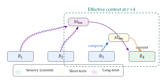
(He et al., 2024 [13].) Given a sequence segmented into blocks $B_{1}, B_{2}, \dots$ of size $s$ , the Hierarchical Memory Transformer (HMT) maintains three memory tiers:

Sensory memory: the raw tokens of the current segment $B_{t}$ , comprising $s$ tokens.
Short-term memory ( $M_{stm}$ ): $k_{stm}$ compressed tokens distilled from the previous segment $B_{t - 1}$ .
Long-term memory ( $M_{ltm}$ ): $k_{ltm}$ compressed tokens aggregating information from all earlier segments $B_{1}, \dots, B_{t - 2}$ .

At each step the effective context is the concatenation $[M_{ltm}; M_{stm}; B_{t}] \in ℝ^{(k_{ltm} + k_{stm} + s) \times d},$ so that the attention cost per segment is $O ((k_{ltm} + k_{stm} + s)^{2} d)$ regardless of total sequence length.

The key operation connecting tiers is memory compression: converting a variable-length token sequence into a fixed number of summary tokens.

Definition 14 (Memory Compression Operator).

A memory compression operator $Compress : ℝ^{n \times d} \to ℝ^{k \times d}$ maps $n$ token representations to $k ≪ n$ memory tokens via learned cross-attention: $M_{compressed} = softmax (\frac{Q_{mem} K_{input}^{⊤}}{\sqrt{d}}) V_{input},$ where $Q_{mem} \in ℝ^{k \times d}$ are learnable query vectors (independent of the input), and $K_{input}, V_{input} \in ℝ^{n \times d}$ are the key and value projections of the input tokens.

Remark 15.

The compression operator is a form of Perceiver-style cross-attention [14]. The learnable queries act as “memory slots” that attend to the input, selecting and mixing the most relevant information. Unlike pooling, the queries can specialise: one slot may capture positional structure while another captures semantic content.

Proposition 6 (HMT Memory Efficiency).

For a sequence of total length $n$ processed in segments of size $s$ , HMT achieves an effective compression ratio of $ρ = \frac{n}{k_{ltm} + k_{stm} + s} .$ Adding only $0.5$ – $1.3 %$ additional parameters as a plug-and-play wrapper around a frozen base model, HMT achieves language modelling quality comparable to long-context models with $2$ – $57 \times$ more parameters, while using $2.5$ – $116 \times$ less inference memory.

Proof.

By induction on segments. At segment $t$ , the model processes $s$ new tokens with an attention context of size $k_{ltm} + k_{stm} + s$ , while having observed $t \cdot s$ total tokens. The ratio $t \cdot s / (k_{ltm} + k_{stm} + s)$ grows linearly with $t$ , establishing the compression ratio. The parameter overhead comes solely from the learnable queries $Q_{mem} \in ℝ^{k \times d}$ at each layer, totalling $L (k_{stm} + k_{ltm}) d$ additional parameters, a fraction $L (k_{stm} + k_{ltm}) d / N_{model}$ of the base model size.

∎

HMT segment-by-segment processing. At segment

B_{4}

, the model attends over its raw tokens (sensory memory, green), a compressed summary of

B_{3}

(short-term memory, amber), and an aggregated summary of

B_{1}, B_{2}

(long-term memory, purple). Wavy arrows denote compression via cross-attention (Definition 14).

H-MEM: Index-Based Hierarchical Routing

Definition 15 (H-MEM).

(Sun & Zeng, 2025 [15].) H-MEM organises the memory of an LLM agent into four nested levels, which the authors describe as analogous to a section, subsection, subsubsection and its content:

(Episode). The stored content itself: individual interaction episodes. Capacity $C_{0}$ , access time $O (1)$ .
(Memory Trace). Groups of related episodes sharing a common thread. Capacity $C_{1}$ .
(Category). Groups of related traces. Capacity $C_{2}$ .
(Domain). The top-level partition of the memory store. Capacity $C_{3}$ .

The cognitive taxonomy of The Cognitive Memory Hierarchy is a useful analogy for why a hierarchy helps, but it is not this architecture's own decomposition: H-MEM's levels are organisational, not functional, and retrieval descends from the broadest partition to the individual episode.

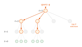
Each level $ℓ$ maintains a set of index nodes ${{𝐢 𝐝 𝐱}_{ℓ} (i)}_{i = 1}^{n_{ℓ}}$ , where ${𝐢 𝐝 𝐱}_{ℓ} (i) \in ℝ^{d}$ is an embedding summarising the content reachable via node $i$ . The index nodes form a tree with branching factor $b$ : each level- $ℓ$ node has $b$ children at level $ℓ - 1$ .

Retrieval in H-MEM is a top-down, beam-search-like traversal of the index tree.

Definition 16 (Recursive Top- $k$ Traversal).

Given a query vector $𝒒 \in ℝ^{d}$ , retrieval proceeds top-down through the hierarchy: $Retrieve (𝒒, ℓ, i) = {\begin{matrix} LeafLookup (𝒒, i) & if ℓ = 0, \\ ⋃_{j \in top- k_{ℓ} (Child (i))} Retrieve (𝒒, ℓ - 1, j) & if ℓ > 0, \end{matrix}$ where $i$ is the parent node reached at the previous level, $Child (i)$ is its set of $b$ children, $S_{ℓ} (j) = \cos (𝒒, {𝐢 𝐝 𝐱}_{ℓ} (j))$ is the cosine similarity between the query and index node $j$ , and $top- k_{ℓ}$ selects the $k_{ℓ}$ highest-scoring children. Restricting the top- $k$ to $Child (i)$ rather than to all level- $ℓ$ nodes is what makes the traversal a descent rather than a flat scan, and is what Proposition 7 depends on. The search begins at the root, $Retrieve (𝒒, L, root)$ .

Proposition 7 (H-MEM Retrieval Complexity).

With $L$ levels, branching factor $b$ , and uniform top- $k$ selection at each level, retrieval requires $O (L \cdot k \cdot b)$ similarity computations, versus $O (b^{L})$ for exhaustive flat search.

Proof.

At each level $ℓ$ , we expand the $k$ selected nodes, each with $b$ children at level $ℓ - 1$ . Computing the similarity score for all $k \cdot b$ children costs $O (k b)$ inner products. Repeating across $L$ levels gives $O (L k b)$ . In contrast, a flat search over all $b^{L}$ leaf nodes requires $O (b^{L})$ comparisons. Since $L k b ≪ b^{L}$ for typical values ( $L = 4$ , $k = 5$ , $b = 100$ gives $2000 ≪ 10^{8}$ ), the hierarchical traversal yields an exponential speedup.

∎

H-MEM retrieval via recursive top-

k

traversal. The query

𝒒

enters at the root (level 3) and selects the

k

most relevant index nodes (orange) at each level, expanding only their children. Leaf nodes (green, level 0) contain the actual memory entries.

Hierarchical FFN Memory Banks

While HMT and H-MEM operate at the sequence level, a complementary approach embeds hierarchical memory directly into the feedforward layers of the Transformer.

Definition 17 (FFN Memory Bank).

(Pouransari et al., 2025 [16].) An external memory bank $ℳ = {(𝒌_{i}, 𝒗_{i})}_{i = 1}^{N_{b}}$ of $N_{b}$ key-value pairs, with $𝒌_{i}, 𝒗_{i} \in ℝ^{d}$ . For a hidden state $𝒉 \in ℝ^{d}$ , the memory-augmented FFN output is: $MemFFN (𝒉) = \sum_{j \in top- k (𝒉^{⊤} K)} α_{j} 𝒗_{j}, α_{j} = \frac{\exp (𝒉^{⊤} 𝒌_{j})}{\sum_{j^{'} \in top- k (𝒉^{⊤} K)} \exp (𝒉^{⊤} 𝒌_{j^{'}})},$ where $K = {[𝒌_{1}, \dots, 𝒌_{N_{b}}]}^{⊤} \in ℝ^{N_{b} \times d}$ is the key matrix. In practice, approximate nearest-neighbour search (e.g., product quantisation) makes the top- $k$ retrieval sub-linear.

The key empirical finding is that a small anchor model augmented with a large memory bank can match substantially larger models.

Proposition 8 (Anchor-Memory Efficiency).

Suppose the knowledge required by a language model follows a Zipf distribution with exponent $s > 1$ over “knowledge units.” Let $N_{a}$ denote the capacity of the anchor model (encoding frequent knowledge) and $N_{b}$ the memory bank size (encoding rare knowledge). The fraction of tokens requiring a memory access scales as $p_{mem} = \sum_{r > N_{a}} \frac{r^{- s}}{ζ (s)} \approx \frac{N_{a}^{- (s - 1)}}{(s - 1) ζ (s)} = O (N_{a}^{- (s - 1)}),$ which decreases as the anchor grows, and does not depend on $N_{b}$ so long as the bank covers the tail. The decay is slow: for typical natural-language distributions $s \approx 1.07$ , so the exponent is only $0.07$ , and this is exactly why the bank has to be large. At those values a 160M anchor model with 18M parameters fetched from a 4.6B-parameter memory bank matches a $2 \times$ -larger standard model in perplexity.

Insight.

HMT, H-MEM, and FFN memory banks all implement the same foundational principle: recent or frequent information resides in fast, small memory; old or rare information resides in slow, large memory. This is precisely the CPU cache hierarchy (L1/L2/L3/DRAM) applied to neural architectures. The “access frequency” analogue shifts from memory addresses to semantic relevance, but the mathematical structure of capacity–latency trade-offs is identical.

Example 5 (Sizing an HMT System).

Consider a 7B-parameter LLM with $d = 4096$ , $L = 32$ layers, deployed for a conversational agent needing 100K-token context. With segment size $s = 2048$ , $k_{stm} = 64$ , $k_{ltm} = 32$ :

Number of segments: $⌈ 100,000 / 2048 ⌉ = 49$ .
Effective context per segment: $64 + 32 + 2048 = 2144$ tokens.
Compression ratio: $100,000 / 2144 \approx 46.6 \times$ .
Added parameters: $32 \times (64 + 32) \times 4096 = 12.6$ M, roughly $0.18 %$ of the base model.
KV cache savings. With $h = 32$ heads of dimension $d_{k} = 128$ , one token costs $2 \times 32 \times 32 \times 128 \times 2 = 524,288$ bytes, that is $512$ ,KiB. Standard attention holds all $49 \times 2048 = 100,352$ tokens, requiring $100,352 \times 524,288 = 52.6$ ,GB ( $49.0$ ,GiB) in fp16, while HMT holds only $2,144$ tokens, requiring $2,144 \times 524,288 = 1.12$ ,GB ( $1.05$ ,GiB). The ratio is $46.8 \times$ , matching the compression ratio above.

Note that the $0.18 %$ parameter overhead here sits below the $0.5$ – $1.3 %$ range quoted in Proposition 6, which reflects larger $k$ values and per-layer memory modules than this minimal configuration uses.

State-Space Models and Recurrent Memory

The architectures of Hierarchical Memory Architectures compress past context into a small set of “summary tokens” accessed via cross-attention. State-space models (SSMs) take this idea to its logical extreme: the entire history is compressed into a single fixed-dimensional state vector, updated recurrently at each time step. This eliminates the quadratic attention cost entirely, but raises a fundamental question: how much of the past can a finite-dimensional state actually remember?

Linear State-Space Models

Definition 18 (Linear State-Space Model).

(Gu et al., 2022 [17].) A continuous-time linear state-space model is a dynamical system (SSM Continuous State) $\begin{matrix} \dot{𝒉} (t) & = A 𝒉 (t) + B 𝒙 (t), \\ 𝒚 (t) & = C 𝒉 (t) + D 𝒙 (t), \end{matrix}$ where $𝒉 (t) \in ℝ^{d_{h}}$ is the hidden state, $𝒙 (t) \in ℝ^{d_{x}}$ is the input, $𝒚 (t) \in ℝ^{d_{y}}$ is the output, and $A \in ℝ^{d_{h} \times d_{h}}$ , $B \in ℝ^{d_{h} \times d_{x}}$ , $C \in ℝ^{d_{y} \times d_{h}}$ , $D \in ℝ^{d_{y} \times d_{x}}$ are learnable parameters. Discretised via zero-order hold with step size $Δ > 0$ : (SSM Discretise A) $\begin{matrix} \overline{A} & = \exp (Δ A), \\ \overline{B} & = (Δ A)^{- 1} (\exp (Δ A) - I) \cdot Δ B . \end{matrix}$ The resulting discrete-time recurrence is (SSM Discrete State) $\begin{matrix} 𝒉_{k} & = \overline{A} 𝒉_{k - 1} + \overline{B} 𝒙_{k}, \\ 𝒚_{k} & = C 𝒉_{k} + D 𝒙_{k} . \end{matrix}$

The remarkable property of linear SSMs is that the same model admits two equivalent computational modes: a recurrent mode for efficient inference and a convolutional mode for parallelised training.

Proposition 9 (Convolution-Recurrence Duality).

The output of the discrete SSM – can be computed as a (non-circular) convolution: $𝒚 = \overline{K} * 𝒙, {\overline{K}}_{j} = C {\overline{A}}^{j} \overline{B}, j = 0, 1, \dots, n - 1,$ where $\overline{K} \in ℝ^{n}$ is the SSM convolution kernel. Training uses FFT-based convolution in $O (n \log n)$ time; inference uses the recurrent form in $O (1)$ time per step with $O (d_{h})$ state.

Proof.

Initialise $𝒉_{0} = 0$ . Unrolling the recurrence : $𝒉_{k} = \sum_{j = 1}^{k} {\overline{A}}^{k - j} \overline{B} 𝒙_{j},$ where the sum runs from $j = 1$ because feeds $𝒙_{k}$ into $𝒉_{k}$ at the same index, so the current input is included and $\overline{A}$ is applied $k - j$ times to the input at step $j$ . Substituting into (with $D = 0$ for clarity): $𝒚_{k} = C 𝒉_{k} = \sum_{j = 1}^{k} C {\overline{A}}^{k - j} \overline{B} 𝒙_{j} = \sum_{m = 0}^{k - 1} {\overline{K}}_{m} 𝒙_{k - m} = {(\overline{K} * 𝒙)}_{k},$ where ${\overline{K}}_{m} = C {\overline{A}}^{m} \overline{B}$ . The convolution can be evaluated for all $k$ simultaneously via the FFT in $O (n \log n)$ .

∎

Remark 16.

The kernel ${\overline{K}}_{j} = C {\overline{A}}^{j} \overline{B}$ decays exponentially when all eigenvalues of $\overline{A}$ have modulus strictly less than $1$ . The S4 model [17] addresses this by initialising $A$ with a special HiPPO (High-order Polynomial Projection Operator) structure [18] that optimally approximates a sliding-window history polynomial, ensuring slow spectral decay and long-range memory. This connects directly to the dynamical systems analysis of Connection to Dynamical Systems.

From S4 to Mamba: Content-Based Selection

Linear SSMs have a critical limitation: since $A$ , $B$ , $C$ are fixed (input-independent), the model treats every token identically; it cannot selectively attend to relevant inputs or ignore irrelevant ones. Mamba resolves this by making the SSM parameters input-dependent.

Definition 19 (Selective State Spaces (Mamba)).

(Gu & Dao, 2023 [19].) Mamba modifies the standard SSM by making the discretisation parameters functions of the input: (Mamba Selection) $\begin{matrix} B_{k} & = f_{B} (𝒙_{k}), & C_{k} & = f_{C} (𝒙_{k}), & Δ_{k} & = softplus (f_{Δ} (𝒙_{k})), \end{matrix}$ where $f_{B}$ , $f_{C}$ , and $f_{Δ}$ are learned linear projections. The discretised matrices become step-dependent: ${\overline{A}}_{k} = \exp (Δ_{k} A)$ , ${\overline{B}}_{k} = {(Δ_{k} A)}^{- 1} (\exp (Δ_{k} A) - I) Δ_{k} B_{k}$ . The recurrence becomes (Mamba Recurrence) $\begin{matrix} 𝒉_{k} = {\overline{A}}_{k} 𝒉_{k - 1} + {\overline{B}}_{k} 𝒙_{k} . \end{matrix}$ This selection mechanism breaks the convolution structure (since ${\overline{A}}_{k}$ now varies per step) but enables content-based memory routing: the model can selectively write to or read from its state based on the input content.

Remark 17.

By making $Δ_{k}$ input-dependent, Mamba effectively learns when to write to its state and when to maintain it:

Large $Δ_{k}$ : ${\overline{A}}_{k} \approx 0$ , so the state is reset and the new input is written strongly.
Small $Δ_{k}$ : ${\overline{A}}_{k} \approx I$ , so the state is preserved and the input is largely ignored.

This is directly analogous to the forget and input gates of LSTMs [20], but operates in continuous time and is parameterised more parsimoniously. The connection to the dynamical systems perspective of Connection to Dynamical Systems is immediate: Mamba implements a time-varying linear dynamical system whose stability properties change adaptively with the input.

Example 6 (Mamba Gating Behaviour).

Consider a sentiment analysis task. When processing the token “not,” $f_{Δ}$ outputs a large value, causing the state to reset and begin accumulating the negated sentiment. When processing filler words like “the” or “a,” $f_{Δ}$ outputs a small value, preserving the current state. This selective gating allows Mamba to match attention-based models on tasks requiring content-dependent routing, while maintaining $O (1)$ per-step cost.

The Attention-Recurrence Trade-off

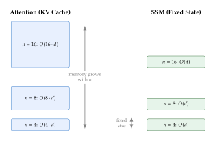
Proposition 10 (SSM Memory Capacity Bound).

The SSM state $𝒉 \in ℝ^{d_{h}}$ can store at most $O (d_{h} \log (1 / ϵ))$ bits of information about the past, where $ϵ$ is the representation precision. For a sequence of length $n$ where each token carries $H$ bits of task-relevant information, faithful memory requires $d_{h} = Ω (\frac{n H}{\log (1 / ϵ)}) .$ In contrast, attention with a full KV cache stores $O (n d)$ parameters, enabling exact recall of any past token.

Proof.

The state $𝒉 \in ℝ^{d_{h}}$ is a vector of $d_{h}$ real numbers, each represented to precision $ϵ$ . Each coordinate stores at most $\log_{2} (1 / ϵ)$ bits, giving a total capacity of $d_{h} \log_{2} (1 / ϵ)$ bits. By the data processing inequality, no function of $𝒉$ can recover more information about the input sequence than $𝒉$ itself contains. For $n$ tokens at $H$ bits each, perfect recall requires $n H$ bits, yielding the stated lower bound on $d_{h}$ .

∎

Attention stores the full KV cache, growing linearly with sequence length

n

. SSMs compress all history into a fixed-size state

𝒉 \in ℝ^{d_{h}}

, sacrificing exact recall for constant memory.

Caution.

SSMs sacrifice precise token-level recall for fixed memory cost. For tasks requiring exact retrieval (e.g., “What was the 5th word in the 3rd paragraph?”), attention-based models substantially outperform SSMs. Hybrid architectures like Jamba [21] address this by interleaving Mamba layers (cheap, providing broad context coverage) with attention layers (expensive, providing precise token recall). The resulting model enjoys the efficiency of SSMs for the majority of layers while retaining the recall capability of attention where needed.

Proposition 11 (Hybrid SSM-Attention Efficiency).

A hybrid model with $L_{ssm}$ Mamba layers and $L_{attn}$ attention layers, processing a sequence of length $n$ :

Memory: $L_{ssm} \cdot d_{h} + L_{attn} \cdot 2 n d_{k}$ (state for SSM layers, KV cache for attention layers).
Computation: $L_{ssm} \cdot O (n d_{h}) + L_{attn} \cdot O (n^{2} d_{k})$ per forward pass.

Setting $L_{attn} / (L_{ssm} + L_{attn}) = r$ , the memory scales as $O (r n + (1 - r) 1) \cdot d$ per layer. Jamba uses $r \approx 1 / 8$ , one attention layer per eight, which by the same expression gives an $8 \times$ smaller KV cache than an all-attention model of comparable size: $4$ ,GB against Mixtral's $32$ ,GB at 256K context, and against $86$ ,GB for LLaMA-2 70B. Retrieval quality on needle-in-a-haystack style tasks is retained at that ratio.

Connections and Synthesis

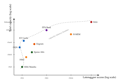
Having surveyed the landscape of memory mechanisms, from grouped-query attention and sliding windows (def:gqa,def:sparse-pattern,def:sliding-window) through external memory systems (def:external-memory,def:engram), hierarchical architectures (def:hmt,def:hmem,def:ffn-memory), and state-space models (def:ssm,def:mamba), we now seek a unifying mathematical framework.

The Memory System Framework

Definition 20 (Memory System).

A memory system is a tuple $(ℳ_{1}, \dots, ℳ_{L}, ϕ)$ where:

Each memory tier $ℳ_{ℓ} = (C_{ℓ}, τ_{ℓ}, A_{ℓ})$ specifies a capacity $C_{ℓ} \in ℝ_{> 0}$ (in tokens or bytes), access latency $τ_{ℓ} \in ℝ_{> 0}$ , and access pattern $A_{ℓ} \in {content, pattern, state, retrieval}$ .
The routing function $ϕ : 𝒬 \to 2^{{1, \dots, L}}$ assigns each query $q \in 𝒬$ to one or more memory tiers.

We require the hierarchy condition: $C_{1} \leq C_{2} \leq \dots \leq C_{L}$ and $τ_{1} \leq τ_{2} \leq \dots \leq τ_{L}$ (faster tiers are smaller).

Theorem 3 (Memory-Computation Trade-off).

Consider a memory system $(ℳ_{1}, \dots, ℳ_{L}, ϕ)$ holding $n$ distinct items, where item $i$ is accessed with probability $π_{i}$ and the items are indexed so that $π_{1} \geq π_{2} \geq \dots \geq π_{n}$ . An assignment is a map $σ : {1, \dots, n} \to {1, \dots, L}$ obeying the capacities, $| σ^{- 1} (ℓ) | \leq C_{ℓ}$ for every $ℓ$ , and its expected access latency is $\overline{τ} (σ) = \sum_{i = 1}^{n} π_{i} τ_{σ (i)} .$ Assume $\sum_{ℓ} C_{ℓ} \geq n$ , so at least one feasible assignment exists. Then the greedy assignment minimises $\overline{τ}$ : place the $C_{1}$ most frequently accessed items in tier 1, the next $C_{2}$ in tier 2, and so on, filling each tier to capacity before spilling into the next.

Proof.

Let $σ$ be any optimal assignment and suppose it is not greedy. Then there are items $i$ and $j$ with $π_{i} > π_{j}$ but $τ_{σ (i)} > τ_{σ (j)}$ , that is, a more frequently accessed item sitting in a slower tier than a less frequently accessed one. Exchanging their tiers keeps the assignment feasible, since it permutes two items between two tiers and changes no tier's occupancy, and it changes the objective by $(π_{i} - π_{j}) (τ_{σ (j)} - τ_{σ (i)}) < 0,$ strictly decreasing $\overline{τ}$ and contradicting optimality. Hence no such inverted pair exists, which is precisely the statement that $σ$ orders items by $π$ against tiers ordered by $τ$ . Any two assignments with that property differ only by permutations within a tier, which leave $\overline{τ}$ unchanged, so the greedy assignment is optimal. This is the rearrangement inequality, and the argument uses only $τ_{1} \leq \dots \leq τ_{L}$ ; the capacity ordering plays no part.

∎

Remark 18.

The picture, fill the fast tier and spill, resembles water-filling, but the mathematics is different. Information-theoretic water-filling solves a concave allocation problem in which marginal returns equalise across channels; here the objective is linear and the solution is the greedy rearrangement above. It is also worth noting what goes wrong without the capacity constraints written as occupancy bounds: a relaxed program that only requires $\sum_{ℓ} p_{ℓ} C_{ℓ} \geq n$ with $p_{ℓ} \geq 0$ has its optimum at a single coordinate, the tier minimising $τ_{ℓ} / C_{ℓ}$ , and never spills at all. Nor is that ratio monotone in $ℓ$ : HBM at $(τ, C) = (1, 1)$ and SSD at $(10^{3}, 10^{6})$ give ratios $1$ and $10^{- 3}$ , decreasing, even though both latency and capacity increase.

Unification Table

Table 1 places every memory mechanism studied in this chapter into the framework of Definition 20.

Method	State Space	Capacity	Latency	Access
KV Cache	$ℝ^{n \times d}$	$O (n d)$ , GPU HBM	$O (1)$	Content
MQA/GQA (Definition 17)	$ℝ^{n \times d G / h}$	$O (n d G / h)$ , GPU HBM	$O (1)$	Content
Sparse Attn (Definition 6)	$ℝ^{w \times d}$	$O (w d)$ , GPU	$O (1)$	Pattern
SSM / Mamba (Definition 19)	$ℝ^{d_{h}}$	$O (d_{h})$ , GPU	$O (1)$	State
Engram (Definition 11)	$ℝ^{T \times d}$	$O (T d)$ , CPU/SSD	$O (1)$ hash	N-gram hash
HMT (Definition 13)	$ℝ^{k \times d}$	$O (k d)$ , GPU	$O (1)$	Cross-attn
H-MEM (Definition 15)	Tree-indexed	$O (b^{L})$	$O (L k b)$	Top- $k$ descent
FFN Bank (Definition 17)	$ℝ^{N_{b} \times d}$	$O (N_{b} d)$ , disk	$O (k)$	Top- $k$ sim.
RAG (Definition 12)	Doc. corpus	Unbounded	High	Retrieval

Memory mechanisms unified under the memory system framework (Definition 20). Capacity and latency are per layer for the attention-resident rows; the Engram, FFN-bank and RAG rows describe a single store shared across the model. The access column refines the four values of Definition 20: “content” means queries are routed by learned similarity, and the entries “N-gram hash”, “cross-attn”, “top-

k

descent” and “top-

k

sim.” name the concrete addressing mechanism used to realise it; “pattern” means routing by a fixed sparsity mask; “state” means implicit encoding in a recurrent state.

The Memory Heterogeneity Principle

Key Idea.

The Memory Heterogeneity Principle. No single memory mechanism is optimal for all types of knowledge. Efficient LLM systems combine fast, small memories for recent and frequent access (KV cache, SSM state) with slow, large memories for rare and historical access (Engram, RAG, FFN memory banks). The optimal allocation between tiers is governed by Theorem 3 and follows the same water-filling principle as CPU cache design and information-theoretic channel allocation.

Connections to Reasoning and Diffusion

Memory and reasoning as dual operations.

The recurrence-based reasoning framework of Recurrent Foundations for Iterative Computation iterates an operator $F$ on a state $𝒉$ , producing a sequence $𝒉^{(0)}, F (𝒉^{(0)}), F^{2} (𝒉^{(0)}), \dots$ that converges (under the conditions of Theorem 1) to a fixed point encoding the answer. Memory provides the data that $F$ operates on: attention retrieves relevant tokens, Engram fetches stored knowledge, and SSM state carries compressed history. In this view:

Reasoning adds depth: more iterations of $F$ extract more complex relationships.
Memory adds breadth: more data supplied to $F$ enables it to draw on more evidence.

The Engram U-shaped scaling law (Theorem 2) quantifies this duality: allocating too many parameters to memory (breadth) starves the reasoning module (depth), and vice versa. The optimal split $α^{*}$ is determined by the relative exponents of the compute and memory scaling laws.

Memory in diffusion language models.

Diffusion LMs (sec:diffusion_language) do not use autoregressive KV caches: they process all positions in parallel at each denoising step, recomputing full bidirectional attention. This means the memory cost per denoising step is $O (n^{2} d)$ , dominated by the attention computation rather than a growing cache. The memory challenge for diffusion LMs is therefore different:

Recomputation cost: each of $T$ denoising steps requires a full forward pass with $O (n^{2})$ attention.
No cache reuse: unlike autoregressive models, where prefill computation is amortised over generation steps, diffusion LMs must recompute from scratch at each step.
Opportunity: sparse attention patterns (Definition 6) and SSM-based denoising backbones can reduce the per-step cost, potentially making diffusion LMs more memory-efficient than autoregressive models for long sequences.

Remark 19.

The synthesis above reveals a surprising convergence: techniques originally developed for autoregressive memory management (sparse attention, state compression, hierarchical caching) find direct application in diffusion models, recurrent reasoning systems, and retrieval-augmented generation. The unifying thread is Theorem 3: every system must navigate the same capacity–latency frontier, regardless of the generative paradigm.

Memory landscape: each mechanism occupies a different point in the capacity–latency space (log–log axes). The

x

-axis measures per-access latency; the

y

-axis measures total capacity. The dashed curve traces the Pareto frontier; an optimal system (Theorem 3) combines mechanisms along this frontier, matching the access distribution to the capacity–latency trade-off. SSM/Mamba and GQA are low-latency/low-capacity; RAG and H-MEM offer large capacity at higher latency.

Historical Timeline

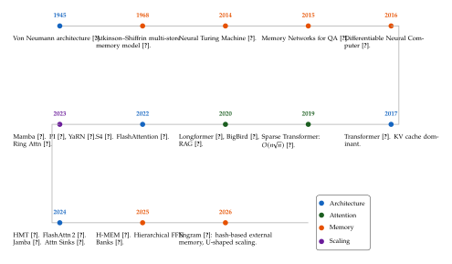
The study of memory in computing and in neural networks has a rich history spanning eight decades. fig:memory-timeline traces the key milestones from the foundational von Neumann architecture through modern hierarchical memory systems. Blue entries denote architectural innovations, green entries denote attention and efficiency methods, orange entries denote memory systems, and purple entries denote scaling and context extension techniques.

Historical timeline of memory-related innovations in computing and neural networks. The progression from static hardware memory hierarchies (1945) through cognitive models (1968) to modern neural memory architectures (2014–2026) reflects a gradual convergence of computer architecture, cognitive science, and deep learning. Colour key: blue = architecture, green = attention method, orange = memory system, purple = scaling/extension.

Exercises

Exercise 8 (KV Cache Arithmetic).

Consider LLaMA-3-405B with $L = 126$ layers, $h = 128$ attention heads, per-head dimension $d_{k} = 128$ , and GQA with $G = 8$ groups (Definition 17).

Compute the KV cache size in GB (fp16, 2 bytes per element) at context lengths $n = 8192$ , $n = 32,768$ , and $n = 131,072$ . Recall from Definition 17 that the $h$ query heads are divided into $G$ groups, each sharing a single key-value head, so the model has $G$ key-value heads in total (and the cache shrinks by the factor $h / G = 16$ ). Hint: each layer stores $2 \times G \times n \times d_{k}$ elements.
The model weights occupy approximately 810,GB in fp16. Compare the KV cache size to the model weight size at each context length.
At what context length does the KV cache exceed the model weights? Express your answer in terms of $L$ , $G$ and $d_{k}$ , and note that $h$ does not appear.

Exercise 9 (Position Interpolation).

Consider RoPE (Definition 15) with base frequency $θ_{base} = 10,000$ and head dimension $d = 128$ .

Compute the rotation frequency $θ_{i} = θ_{base}^{- 2 i / d}$ for $i = 0$ (highest frequency) and $i = 63$ (lowest frequency).
Compute the rotation angle $m θ_{i}$ at position $m = 4096$ for both frequencies from part (a). Express in radians and in number of full rotations.
Apply Position Interpolation (Definition 3) to extend the context from $L_{train} = 4096$ to $L_{target} = 32,768$ (scaling factor $α = 8$ ). Recompute the rotation angles at $m = 32,768$ with the interpolated positions and verify that they fall within the range seen during training at $m = 4096$ .

Exercise 10 (YaRN Temperature).

When applying NTK-aware scaling (Definition 4) with factor $α$ , the attention logits for a query-key pair separated by distance $m$ scale differently across frequency bands.

Starting from $θ_{i}^{'} = θ_{i} α^{- 2 i / (d - 2)}$ , show that the highest-frequency component ( $i = 0$ ) is left unchanged, while the lowest-frequency component ( $i = d / 2 - 1$ ) is compressed by the full factor $α$ .
Argue that the attention entropy increases as the interpolated logit magnitudes contract, and explain why a multiplicative temperature on the logits is the natural correction.
Show that a logit multiplier of the form ${(c \ln α + 1)}^{2}$ can restore the pre-interpolation entropy to first order, and note that YaRN fits $c = 0.1$ empirically for the LLaMA family rather than deriving it. Verify for $α = 8$ that $\sqrt{1 / t} = 0.1 \ln 8 + 1 \approx 1.208$ , so the logits are multiplied by ${1.208}^{2} \approx 1.459$ .

Exercise 11 (BigBird Connectivity).

Consider BigBird (Definition 8) with $g$ global tokens, sliding window of width $w$ , and sequence length $n$ .

Ignoring the global tokens, so that only window edges may be used, prove that information propagates between any two positions in at most $⌈ \frac{n - 2 g}{2 w} ⌉ + 2$ hops.
For $n = 4096$ , $g = 64$ , $w = 128$ , compute that bound.
Now restore the global tokens and apply Theorem 1. How many hops are needed? Compare with your answer to (b) and explain, in one sentence, which structural feature of the pattern accounts for the whole difference.
For a Transformer with $L$ layers, each layer enables one hop. State the condition on $L$ for full connectivity, first with $g \geq 1$ and then with $g = 0$ .

Exercise 12 (Ring Attention Communication).

Consider Ring Attention (Proposition 4) with $P = 8$ devices, sequence length $n = 1,000,000$ tokens, $d_{k} = 128$ , and fp16 precision.

Each device holds $n / P$ tokens. In each of the $P - 1$ communication rounds, each device sends its KV block (of size $2 \times (n / P) \times d_{k}$ elements) to the next device. Compute the total bytes communicated per layer across all rounds and all devices.
On NVLink with 900,GB/s bidirectional bandwidth, estimate the wall-clock communication time per layer. Assume communication is fully overlapped with computation where possible.
Estimate the Flash Attention computation time for $n / P = 125,000$ tokens on an A100 GPU (312 TFLOPS fp16). Is the system compute-bound or communication-bound?

Exercise 13 (Engram Hash Collisions).

Engram (Definition 11) uses a hash table of size $T$ with 2-gram keys drawn from a vocabulary of size $V$ .

Assuming a uniform hash function, compute the expected number of entries per bucket when all $V^{2}$ possible 2-grams are inserted.
What is the probability that two distinct 2-grams $(𝒙_{1}, 𝒙_{2})$ and $(𝒙_{1}^{'}, 𝒙_{2}^{'})$ collide (i.e., map to the same bucket)?
For $V = 50,000$ , require that the probability of at least one collision occurring among all $V^{2}$ inserted 2-grams is below $1 %$ . Using the birthday approximation $1 - e^{- N^{2} / (2 T)}$ with $N = V^{2}$ , what is the minimum table size $T$ ? Is this practical? Contrast it with the far weaker requirement that a single specified pair collide with probability below $1 %$ .
In practice, not all $V^{2}$ 2-grams appear. If only $N_{obs}$ distinct 2-grams occur in the training corpus, how does the collision analysis change? Relate to the birthday paradox.

Exercise 14 (U-Shaped Scaling Optimisation).

The Engram scaling law (Theorem 2) gives the loss as $L (α) = a (α C)^{- p} + b ((1 - α) C)^{- q},$ where $α$ is the fraction of compute allocated to the neural model and $1 - α$ to the memory module. Use $a = 1$ , $b = 0.5$ , $p = 0.07$ , $q = 0.05$ , $C = 10^{10}$ .

Differentiate $L (α)$ with respect to $α$ and set to zero. Show that the optimal split satisfies $\frac{a p}{α^{p + 1}} = \frac{b q}{{(1 - α)}^{q + 1}} \cdot C^{p - q},$ or derive an equivalent implicit equation.
Solve numerically for $α^{*}$ . Verify that $L (α^{*})$ is a minimum (not a maximum) by checking the second derivative.
How does $α^{*}$ change as $C$ increases from $10^{8}$ to $10^{14}$ ? Plot $α^{*} (C)$ and interpret the trend: does a larger budget favour more memory or more compute?

Exercise 15 (HMT Compression Analysis).

A document of $100,000$ tokens is processed by HMT with segment size $s = 2048$ , $k_{stm} = 64$ , and $k_{ltm} = 16$ .

How many segments are needed to process the full document?
What is the compression ratio $ρ = n / (k_{ltm} + k_{stm} + s)$ ?
Each compression step (Definition 14) retains a fraction $1 - ϵ$ of the information, with $ϵ = 0.05$ . After 20 segments, what fraction of the original information from segment 1 remains in long-term memory?
At what number of segments does the retained information drop below $50 %$ ? Below $10 %$ ? What are the implications for very long documents?

Exercise 16 (H-MEM Retrieval Analysis).

An H-MEM system has $L = 4$ levels, branching factor $b = 100$ , and uniform top- $k = 5$ selection at each level.

What is the total memory capacity (number of leaf entries)?
How many similarity computations are required per query?
What is the speedup over flat (exhaustive) search?
If each similarity computation takes 100,ns, what is the retrieval latency? Compare to a flat search over $10^{8}$ entries.

Exercise 17 (SSM Memory Capacity).

Consider a Mamba model with state dimension $d_{h} = 2048$ and fp16 precision ( $ϵ = 2^{- 10}$ for the significand).

Using Proposition 10, compute the maximum number of bits storable in the state.
For a 128K-token sequence where each token carries $H = 8$ bits of task-relevant information, what fraction of the total information can the state represent?
Design a hybrid architecture: Mamba for $90 %$ of layers, attention for $10 %$ of layers (each with full KV cache). For a model with $L = 32$ layers and $d = 4096$ , compute the total memory at $n = 128$ K tokens. What are the savings compared to full attention?

Exercise 18 (Convolution-Recurrence Duality).

Starting from the discrete SSM recurrence $𝒉_{k} = \overline{A} 𝒉_{k - 1} + \overline{B} 𝒙_{k}$ with $𝒉_{0} = 0$ :

Prove by induction that $𝒚_{k} = \sum_{j = 1}^{k} C {\overline{A}}^{k - j} \overline{B} 𝒙_{j} = \sum_{m = 0}^{k - 1} {\overline{K}}_{m} 𝒙_{k - m}$ with ${\overline{K}}_{m} = C {\overline{A}}^{m} \overline{B}$ . Check the case $k = 1$ against the recurrence before generalising.
What condition on the eigenvalues ${λ_{i}}$ of $\overline{A}$ ensures that the convolution kernel ${\overline{K}}_{m} = C {\overline{A}}^{m} \overline{B}$ decays exponentially?
Relate the eigenvalue condition to the vanishing gradient problem in RNNs. Why does the HiPPO initialisation help?
Show that if $\overline{A}$ is diagonal with entries ${\overline{a}}_{1}, \dots, {\overline{a}}_{d_{h}}$ , the kernel $\overline{K}$ can be evaluated in $O (d_{h} n)$ time without matrix powers.

Exercise 19 (Memory Bandwidth Analysis).

Consider an A100 GPU with 2,TB/s HBM bandwidth (Definition 2) and a KV cache of 10,GB.

During autoregressive generation, each token requires reading the entire KV cache. What is the maximum generation rate (tokens/second), ignoring computation time?
The model has $h = 32$ attention heads. With GQA (Definition 17) using $G = 8$ groups, so that there are $G = 8$ key-value heads shared among the $32$ query heads, the cache shrinks by the factor $h / G = 4$ , to $10 / 4 = 2.5$ ,GB. What is the new generation rate?
Suppose we offload $80 %$ of the KV cache to CPU memory, accessible via PCIe 5.0 at 64,GB/s. The remaining $20 %$ stays in HBM. What is the effective bandwidth, assuming uniform access? What is the generation rate?
At what offloading fraction does the system become communication-bound (CPU bandwidth limits throughput)?

Exercise 20 (RAG as a Memory System).

Map Retrieval-Augmented Generation (Definition 12) into the memory system framework of Definition 20.

Identify the memory tiers. What is the “fast tier” and what is the “slow tier”? What are their capacities and latencies?
What is the routing function $ϕ$ ? How does it decide which queries go to the retrieval tier?
Compare RAG's memory system to Engram's (Definition 11). What are the key differences in routing, latency, and integration depth?
Under what conditions does Theorem 3 predict that RAG outperforms a larger model without retrieval?

Exercise 21 (Engram vs. Mixture of Experts).

Compare two approaches to scaling knowledge capacity:

Engram: a hash table with $T$ entries, each of dimension $d$ , totalling $T d$ parameters. Lookup is $O (1)$ via hashing.
Mixture of Experts (MoE): $E$ experts, each an FFN with $2 d^{2}$ parameters, totalling $2 E d^{2}$ parameters. Top- $k$ routing costs $O (E d)$ for the gating computation.

Express the total parameter count and per-token FLOP cost for each approach.
Under what relationship between $T$ , $E$ , and $d$ does Engram store more parameters per FLOP of lookup cost?
MoE experts can compute with their parameters (via the FFN), while Engram entries are passively retrieved. Discuss the qualitative implications: when is passive retrieval sufficient, and when is active computation necessary?
Propose a hybrid “Engram-of-Experts” architecture that uses hash-based routing to select experts. What are the potential benefits and challenges?

Exercise 22 (Open Problem: Optimal Memory Architecture).

Given a total parameter budget $N$ , a target context length $n$ , and a task distribution $𝒯$ :

Formalise the problem of finding the optimal memory architecture as an optimisation problem. Your decision variables should include: the number of tiers $L$ , the capacity $C_{ℓ}$ and access mechanism $A_{ℓ}$ of each tier, and the routing function $ϕ$ . Your objective should minimise the expected loss on $𝒯$ .
Why is this optimisation problem computationally hard? Identify at least three sources of difficulty (combinatorial structure, non-convexity, distribution dependence, etc.).
Using the insight from the U-shaped scaling law (Theorem 2), propose a practical heuristic: (i) estimate the scaling exponents $p$ and $q$ from small-scale experiments, (ii) compute the optimal split $α^{*}$ , and (iii) allocate tiers greedily along the Pareto frontier of fig:memory-landscape. Under what assumptions is this heuristic near-optimal?

References

Neural Turing Machines

Alex Graves, Greg Wayne, Ivo Danihelka

arXiv preprint arXiv:1410.5401 · 2014

BibTeX

@article{graves2014neural,
  title={Neural Turing Machines},
  author={Graves, Alex and Wayne, Greg and Danihelka, Ivo},
  journal={arXiv preprint arXiv:1410.5401},
  year={2014}
}

Journal article

Memory Networks

Jason Weston, Sumit Chopra, Antoine Bordes

International Conference on Learning Representations · 2015

BibTeX

@inproceedings{weston2015memory,
  title={Memory Networks},
  author={Weston, Jason and Chopra, Sumit and Bordes, Antoine},
  booktitle={International Conference on Learning Representations},
  year={2015}
}

Conference paper

Extending Context Window of Large Language Models via Positional Interpolation

Shouyuan Chen, Sherman Wong, Liangjian Chen, Yuandong Tian

arXiv preprint arXiv:2306.15595 · 2023

BibTeX

@article{chen2023extending,
  title={Extending Context Window of Large Language Models via Positional Interpolation},
  author={Chen, Shouyuan and Wong, Sherman and Chen, Liangjian and Tian, Yuandong},
  journal={arXiv preprint arXiv:2306.15595},
  year={2023}
}

Journal article

YaRN: Efficient Context Window Extension of Large Language Models

Bowen Peng, Jeffrey Quesnelle, Honglu Fan, Enrico Shippole

arXiv preprint arXiv:2309.00071 · 2024

BibTeX

@article{peng2024yarn,
  title={{YaRN}: Efficient Context Window Extension of Large Language Models},
  author={Peng, Bowen and Quesnelle, Jeffrey and Fan, Honglu and Shippole, Enrico},
  journal={arXiv preprint arXiv:2309.00071},
  year={2024}
}

Journal article

BigBird: Transformers for Longer Sequences

Manzil Zaheer, Guru Guruganesh, Kumar Avinava Dubey, Joshua Ainslie, Chris Alberti, Santiago Ontanon, others

Advances in Neural Information Processing Systems, vol. 33 · 2020

BibTeX

@inproceedings{zaheer2020bigbird,
  title={{BigBird}: Transformers for Longer Sequences},
  author={Zaheer, Manzil and Guruganesh, Guru and Dubey, Kumar Avinava and Ainslie, Joshua and Alberti, Chris and Ontanon, Santiago and others},
  booktitle={Advances in Neural Information Processing Systems},
  volume={33},
  year={2020}
}

Conference paper

Hybrid Computing Using a Neural Network with Dynamic External Memory

Alex Graves, Greg Wayne, Malcolm Reynolds, Tim Harley, Ivo Danihelka, Agnieszka Grabska-Barwinska, others

Nature, vol. 538, no. 7626, pp. 471-476 · 2016

BibTeX

@article{graves2016hybrid,
  title={Hybrid Computing Using a Neural Network with Dynamic External Memory},
  author={Graves, Alex and Wayne, Greg and Reynolds, Malcolm and Harley, Tim and Danihelka, Ivo and Grabska-Barwi{\'n}ska, Agnieszka and others},
  journal={Nature},
  volume={538},
  number={7626},
  pages={471--476},
  year={2016}
}

Journal article

Outrageously Large Neural Networks: The Sparsely-Gated Mixture-of-Experts Layer

Noam Shazeer, Azalia Mirhoseini, Krzysztof Maziarz, Andy Davis, Quoc Le, Geoffrey Hinton, Jeff Dean

International Conference on Learning Representations · 2017

BibTeX

@inproceedings{shazeer2017outrageously,
  title={Outrageously Large Neural Networks: The Sparsely-Gated Mixture-of-Experts Layer},
  author={Shazeer, Noam and Mirhoseini, Azalia and Maziarz, Krzysztof and Davis, Andy and Le, Quoc and Hinton, Geoffrey and Dean, Jeff},
  booktitle={International Conference on Learning Representations},
  year={2017}
}

Conference paper

Retrieval-Augmented Generation for Knowledge-Intensive NLP Tasks

Patrick Lewis, Ethan Perez, Aleksandra Piktus, Fabio Petroni, Vladimir Karpukhin, Naman Goyal, others

Advances in Neural Information Processing Systems, vol. 33 · 2020

BibTeX

@article{lewis2020retrieval,
  title={Retrieval-Augmented Generation for Knowledge-Intensive {NLP} Tasks},
  author={Lewis, Patrick and Perez, Ethan and Piktus, Aleksandra and Petroni, Fabio and Karpukhin, Vladimir and Goyal, Naman and others},
  journal={Advances in Neural Information Processing Systems},
  volume={33},
  year={2020}
}

Journal article

Human Memory: A Proposed System and Its Control Processes

Richard C. Atkinson, Richard M. Shiffrin

Psychology of Learning and Motivation, vol. 2, pp. 89-195 · 1968

BibTeX

@article{atkinson1968human,
  title={Human Memory: A Proposed System and Its Control Processes},
  author={Atkinson, Richard C. and Shiffrin, Richard M.},
  journal={Psychology of Learning and Motivation},
  volume={2},
  pages={89--195},
  year={1968}
}

Journal article

Working Memory

Alan D. Baddeley, Graham Hitch

Psychology of Learning and Motivation, vol. 8, pp. 47-89 · 1974

BibTeX

@article{baddeley1974working,
  title={Working Memory},
  author={Baddeley, Alan D. and Hitch, Graham},
  journal={Psychology of Learning and Motivation},
  volume={8},
  pages={47--89},
  year={1974}
}

Journal article

Episodic and Semantic Memory

Endel Tulving

Organization of Memory, pp. 381-403 · 1972

BibTeX

@article{tulving1972episodic,
  title={Episodic and Semantic Memory},
  author={Tulving, Endel},
  journal={Organization of Memory},
  pages={381--403},
  year={1972},
  publisher={Academic Press}
}

Journal article

The Magical Number Seven, Plus or Minus Two: Some Limits on Our Capacity for Processing Information

George A. Miller

Psychological Review, vol. 63, no. 2, pp. 81-97 · 1956

BibTeX

@article{miller1956magical,
  title={The Magical Number Seven, Plus or Minus Two: Some Limits on Our Capacity for Processing Information},
  author={Miller, George A.},
  journal={Psychological Review},
  volume={63},
  number={2},
  pages={81--97},
  year={1956}
}

Journal article

HMT: Hierarchical Memory Transformer for Efficient Long Context Language Processing

Zifan He, others

Proceedings of NAACL · 2025

BibTeX

@inproceedings{he2024hmt,
  title={{HMT}: Hierarchical Memory Transformer for Efficient Long Context Language Processing},
  author={He, Zifan and others},
  booktitle={Proceedings of NAACL},
  note={arXiv:2405.06067},
  year={2025}
}

Conference paper

Perceiver: General Perception with Iterative Attention

Andrew Jaegle, Felix Gimeno, Andrew Brock, Andrew Zisserman, Oriol Vinyals, Joao Carreira

International Conference on Machine Learning, pp. 4651-4664 · 2021

BibTeX

@inproceedings{jaegle2021perceiver,
  title={Perceiver: General Perception with Iterative Attention},
  author={Jaegle, Andrew and Gimeno, Felix and Brock, Andrew and Zisserman, Andrew and Vinyals, Oriol and Carreira, Jo{\~a}o},
  booktitle={International Conference on Machine Learning},
  pages={4651--4664},
  year={2021}
}

Conference paper

Hierarchical Memory for High-Efficiency Long-Term Reasoning in LLM Agents

Haoran Sun, Shaoning Zeng

arXiv preprint arXiv:2507.22925 · 2025

BibTeX

@article{sun2025hmem,
  title={Hierarchical Memory for High-Efficiency Long-Term Reasoning in {LLM} Agents},
  author={Sun, Haoran and Zeng, Shaoning},
  journal={arXiv preprint arXiv:2507.22925},
  year={2025}
}

Journal article

Pretraining with Hierarchical Memories: Separating Long-Tail and Common Knowledge

Hadi Pouransari, others

arXiv preprint arXiv:2510.02375 · 2025

BibTeX

@article{pouransari2025hierarchical,
  title={Pretraining with Hierarchical Memories: Separating Long-Tail and Common Knowledge},
  author={Pouransari, Hadi and others},
  journal={arXiv preprint arXiv:2510.02375},
  year={2025}
}

Journal article

Efficiently Modeling Long Sequences with Structured State Spaces

Albert Gu, Karan Goel, Christopher Re

International Conference on Learning Representations · 2022

BibTeX

@article{gu2022efficiently,
  title={Efficiently Modeling Long Sequences with Structured State Spaces},
  author={Gu, Albert and Goel, Karan and R{\'e}, Christopher},
  journal={International Conference on Learning Representations},
  year={2022}
}

Journal article

HiPPO: Recurrent Memory with Optimal Polynomial Projections

Albert Gu, Tri Dao, Stefano Ermon, Atri Rudra, Christopher Re

Advances in Neural Information Processing Systems, vol. 33 · 2020

BibTeX

@article{gu2020hippo,
  title={{HiPPO}: Recurrent Memory with Optimal Polynomial Projections},
  author={Gu, Albert and Dao, Tri and Ermon, Stefano and Rudra, Atri and R{\'e}, Christopher},
  journal={Advances in Neural Information Processing Systems},
  volume={33},
  year={2020}
}

Journal article

Mamba: Linear-Time Sequence Modeling with Selective State Spaces

Albert Gu, Tri Dao

arXiv preprint arXiv:2312.00752 · 2023

BibTeX

@article{gu2023mamba,
  title={Mamba: Linear-Time Sequence Modeling with Selective State Spaces},
  author={Gu, Albert and Dao, Tri},
  journal={arXiv preprint arXiv:2312.00752},
  year={2023}
}

Journal article

Long Short-Term Memory

Sepp Hochreiter, Jurgen Schmidhuber

Neural Computation, vol. 9, no. 8, pp. 1735-1780 · 1997

BibTeX

@article{hochreiter1997long,
  title={Long Short-Term Memory},
  author={Hochreiter, Sepp and Schmidhuber, J{\"u}rgen},
  journal={Neural Computation},
  volume={9},
  number={8},
  pages={1735--1780},
  year={1997}
}

Journal article

Jamba: A Hybrid Transformer-Mamba Language Model

Opher Lieber, Barak Lenz, Horace Bata, Gal Cohen, Jhonathan Osin, others

arXiv preprint arXiv:2403.19887 · 2024

BibTeX

@article{lieber2024jamba,
  title={Jamba: A Hybrid Transformer-Mamba Language Model},
  author={Lieber, Opher and Lenz, Barak and Bata, Horace and Cohen, Gal and Osin, Jhonathan and others},
  journal={arXiv preprint arXiv:2403.19887},
  year={2024}
}

Journal article

Longformer: The Long-Document Transformer

Iz Beltagy, Matthew E. Peters, Arman Cohan

arXiv preprint arXiv:2004.05150 · 2020

BibTeX

@article{beltagy2020longformer,
  title={Longformer: The Long-Document Transformer},
  author={Beltagy, Iz and Peters, Matthew E. and Cohan, Arman},
  journal={arXiv preprint arXiv:2004.05150},
  year={2020}
}

Journal article

Ring Attention with Blockwise Transformers for Near-Infinite Context

Hao Liu, Matei Zaharia, Pieter Abbeel

International Conference on Learning Representations · 2024

BibTeX

@inproceedings{liu2023ring,
  title={Ring Attention with Blockwise Transformers for Near-Infinite Context},
  author={Liu, Hao and Zaharia, Matei and Abbeel, Pieter},
  booktitle={International Conference on Learning Representations},
  note={arXiv:2310.01889, October 2023},
  year={2024}
}

Conference paper

Conditional Memory via Scalable Lookup: A New Axis of Sparsity for Large Language Models

Xin Cheng, others

arXiv preprint arXiv:2601.07372 · 2026

BibTeX

@article{cheng2026engram,
  title={Conditional Memory via Scalable Lookup: A New Axis of Sparsity for Large Language Models},
  author={Cheng, Xin and others},
  journal={arXiv preprint arXiv:2601.07372},
  year={2026}
}

Journal article

← 23 Recurrence, Recursion, and Reasoning 25 Fine-Tuning and Alignment →