23 Recurrence, Recursion, and Reasoning

Can neural networks reason? This question, deceptively simple to state, lies at the very heart of modern artificial intelligence. Generating fluent text is not the same as reasoning about it: a language model may produce a convincing paragraph about prime numbers without being able to check whether $97$ is prime. Generating an image of a chess board is not the same as reasoning about the game: the model may paint every piece in photographic detail yet be unable to determine whether white is in check. The gap between production and reasoning is one of the central intellectual challenges of generative modelling, and it is the subject of this chapter.

We will approach the question mathematically. Rather than debating whether machines “truly” understand, we will ask: what are the computational mechanisms that enable generative models to solve problems requiring multi-step inference, and what are the fundamental mathematical limits of those mechanisms?

Key Idea.

What computational mechanisms enable generative models to reason? And what are the fundamental mathematical limits of these mechanisms? This chapter develops the mathematical framework to answer both questions.

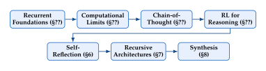
The chapter follows a deliberate arc. We begin with recurrent foundations (Recurrent Foundations for Iterative Computation), revisiting RNNs, LSTMs, and GRUs as iterated maps and connecting them to the theory of dynamical systems and fixed points. We then confront the computational limits of Transformers (Computational Limits of Transformers), showing that a single forward pass through a fixed-depth Transformer computes a function in the circuit complexity class ${𝖳 𝖢}^{0}$ : powerful, but unable to solve certain polynomial-time problems unless the long-standing conjecture ${𝖳 𝖢}^{0} \neq {𝖭 𝖢}^{1}$ fails. This motivates chain-of-thought reasoning (Chain-of-Thought Reasoning), where the model generates intermediate tokens that turn a bounded-depth computation into an unbounded one and carry the model's reach all the way up to $𝖯$ . We then study how reinforcement learning can train models to discover reasoning strategies on their own (Reinforcement Learning for Reasoning), culminating in the GRPO algorithm behind DeepSeek-R1. The later sections address self-reflection (Self-Reflection and Iterative Refinement), recursive architectures (Recursive Reasoning Architectures), and a synthesis of the entire reasoning landscape (Connections and Synthesis).

Historical Note.

The question of machine reasoning has a long pedigree. Alan Turing asked “Can machines think?” in 1950 [1], proposing the imitation game as a test. Jeffrey Elman introduced the Simple Recurrent Network in 1990 [2], showing that recurrence enables networks to process sequential structure. Hochreiter and Schmidhuber's Long Short-Term Memory (1997) [3] solved the vanishing gradient problem and enabled learning over hundreds of time steps. The Transformer (2017) [4] replaced recurrence with attention, unlocking massive parallelism and scaling to billions of parameters. Chain-of-thought prompting (2022) [5] revealed that large language models could solve complex problems by “thinking aloud.” DeepSeek-R1 (2025) [6] demonstrated that reinforcement learning could elicit sophisticated reasoning behaviours, including spontaneous self-correction, without any explicit supervision of the reasoning process.

Roadmap for this chapter. We progress from the mathematical foundations of recurrence, through the computational limits that motivate chain-of-thought, to RL-based training and recursive architectures.

Recurrent Foundations for Iterative Computation

Before we can understand the reasoning capabilities of modern language models, we must understand the mathematical structure of recurrence, the idea that a computation proceeds by repeatedly applying a function to its own output. Recurrence is the oldest and most natural mechanism for iterative computation in neural networks, and its mathematical properties illuminate both the power and the limitations of sequential reasoning.

Recurrence as Iterative Computation

Recall the recurrent neural network defined in Definition 10: given an input sequence $(𝒙_{1}, \dots, 𝒙_{T})$ , the RNN updates a hidden state via (RNN Recall) $\begin{matrix} 𝒉_{t} = σ (W_{h} 𝒉_{t - 1} + W_{x} 𝒙_{t} + 𝒃) . \end{matrix}$ The key observation is that, for a fixed input token $𝒙_{t} = 𝒙$ , the update rule defines a map (RNN MAP) $\begin{matrix} F_{𝒙} : ℝ^{d} \to ℝ^{d}, F_{𝒙} (𝒉) = σ (W_{h} 𝒉 + W_{x} 𝒙 + 𝒃) . \end{matrix}$ Computing $𝒉_{1}, 𝒉_{2}, \dots, 𝒉_{T}$ is then precisely the iterated application of a sequence of maps: $𝒉_{t} = F_{𝒙_{t}} \circ F_{𝒙_{t - 1}} \circ \dots \circ F_{𝒙_{1}} (𝒉_{0})$ . This viewpoint (recurrence as iterated function application) is the foundation upon which the entire chapter rests.

Remark 1 (Autoregressive Generation is Recurrent).

Even the Transformer, which replaces recurrence in its architecture, is recurrent in its generation process. When an autoregressive model generates tokens one at a time, each forward pass takes the concatenation of all previous tokens and produces the next. If we let $𝒔_{t} = (x_{1}, \dots, x_{t})$ denote the state (the sequence generated so far), then the generation step $𝒔_{t + 1} = (𝒔_{t}, x_{t + 1})$ where $x_{t + 1} \sim p_{θ} (\cdot | 𝒔_{t})$ is an iterated stochastic map. The theory of recurrence therefore applies to reasoning in all autoregressive models, not only RNNs.

An RNN unrolled in time. Each green box applies the same function

F

; the hidden state

𝒉_{t}

(blue circles) flows left to right. Inputs

𝒙_{t}

(orange) feed in from below.

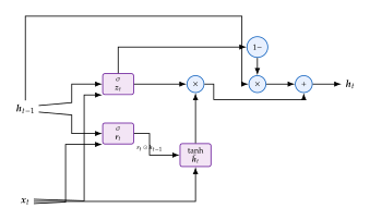
The Gated Recurrent Unit (GRU)

The LSTM (Definition 11) solved the vanishing gradient problem with three gates and a separate cell state. The Gated Recurrent Unit (GRU), introduced by Cho et al. [21], achieves a similar effect with a simpler architecture using only two gates.

Definition 1 (Gated Recurrent Unit (GRU)).

The GRU processes a sequence $(𝒙_{1}, \dots, 𝒙_{T})$ by updating a hidden state $𝒉_{t} \in ℝ^{d}$ via two gates (the update gate $𝒛_{t}$ and the reset gate $𝒓_{t}$ ) and a candidate activation ${\tilde{𝒉}}_{t}$ : (GRU Update) $\begin{matrix} 𝒛_{t} & = σ (W_{z} [𝒉_{t - 1}, 𝒙_{t}] + 𝒃_{z}), & (update gate) \\ 𝒓_{t} & = σ (W_{r} [𝒉_{t - 1}, 𝒙_{t}] + 𝒃_{r}), & (reset gate) \\ {\tilde{𝒉}}_{t} & = \tanh (W_{h} [𝒓_{t} ⊙ 𝒉_{t - 1}, 𝒙_{t}] + 𝒃_{h}), & (candidate) \\ 𝒉_{t} & = (1 - 𝒛_{t}) ⊙ 𝒉_{t - 1} + 𝒛_{t} ⊙ {\tilde{𝒉}}_{t}, & (interpolation) \end{matrix}$ where $σ$ is the element-wise sigmoid, $⊙$ denotes the Hadamard (element-wise) product, and $[𝒉_{t - 1}, 𝒙_{t}]$ denotes concatenation. The weight matrices are $W_{z}, W_{r}, W_{h} \in ℝ^{d \times (d + d_{x})}$ with bias vectors $𝒃_{z}, 𝒃_{r}, 𝒃_{h} \in ℝ^{d}$ .

The crucial design choice is (GRU Update): the new hidden state is a convex interpolation between the old state $𝒉_{t - 1}$ and the candidate ${\tilde{𝒉}}_{t}$ , controlled by the update gate $𝒛_{t}$ . When $𝒛_{t} \approx 0$ , the hidden state is copied unchanged; when $𝒛_{t} \approx 1$ , the hidden state is overwritten with the candidate.

Remark 2 (GRU vs. LSTM).

The GRU has two gates; the LSTM (Definition 11) has three (forget, input, output) plus a separate cell state $𝒄_{t}$ . Despite having fewer parameters, the GRU often matches the LSTM in practice on tasks such as language modelling and speech recognition. The key shared idea is the linear interpolation pathway: the LSTM has $𝒄_{t} = 𝒇_{t} ⊙ 𝒄_{t - 1} + 𝒊_{t} ⊙ {\tilde{𝒄}}_{t}$ , while the GRU has $𝒉_{t} = (1 - 𝒛_{t}) ⊙ 𝒉_{t - 1} + 𝒛_{t} ⊙ {\tilde{𝒉}}_{t}$ . In both cases, when the “copy” gate is close to identity, information flows through unattenuated.

Proposition 1 (GRU Gradient Through the Copy Pathway).

Consider the GRU update . The Jacobian of $𝒉_{t}$ with respect to $𝒉_{t - 1}$ contains the term (GRU Jacobian) $\begin{matrix} \frac{\partial 𝒉_{t}}{\partial 𝒉_{t - 1}} = diag (1 - 𝒛_{t}) + (terms involving \frac{\partial 𝒛_{t}}{\partial 𝒉_{t - 1}} and \frac{\partial {\tilde{𝒉}}_{t}}{\partial 𝒉_{t - 1}}) . \end{matrix}$ When the update gate satisfies $𝒛_{t} \approx 0$ , the dominant term is $diag (1 - 𝒛_{t}) \approx I$ , so the gradient is close to the identity matrix. This provides a gradient highway: gradients flow from $𝒉_{T}$ back to $𝒉_{t}$ without exponential attenuation, as long as the update gates remain small along the path.

Proof.

By the product and chain rules applied to (GRU Update), (GRU Jacobian FULL) $\begin{matrix} \frac{\partial 𝒉_{t}}{\partial 𝒉_{t - 1}} & = diag (1 - 𝒛_{t}) - diag (𝒉_{t - 1} - {\tilde{𝒉}}_{t}) \frac{\partial 𝒛_{t}}{\partial 𝒉_{t - 1}} + diag (𝒛_{t}) \frac{\partial {\tilde{𝒉}}_{t}}{\partial 𝒉_{t - 1}} . \end{matrix}$ When $𝒛_{t} \approx 0$ , the second term is scaled by $(𝒉_{t - 1} - {\tilde{𝒉}}_{t})$ (bounded) times $\partial 𝒛_{t} / \partial 𝒉_{t - 1}$ , whose sigmoid factor evaluated at the gate's own output is $𝒛_{t} ⊙ (1 - 𝒛_{t})$ , and the third term is scaled by $𝒛_{t}$ directly. Both corrections are therefore $O (‖ 𝒛_{t} ‖)$ : they vanish at the same rate as the gate itself, not merely below the sigmoid's global maximum slope of $1 / 4$ . (At $𝒛_{t} = 0.01$ the factor is $0.01 \times 0.99 = 0.0099$ , and the maximum $1 / 4$ is attained at $𝒛_{t} = 1 / 2$ , the opposite regime.) Hence the dominant contribution is $diag (1 - 𝒛_{t}) \approx I$ . Over $T - t$ time steps, the product $\prod_{k = t + 1}^{T} \frac{\partial 𝒉_{k}}{\partial 𝒉_{k - 1}}$ remains close to the identity rather than decaying exponentially, establishing the gradient highway property.

∎

Architecture of the GRU cell. The update gate

𝒛_{t}

controls the interpolation between the previous hidden state

𝒉_{t - 1}

(via the

1 - 𝒛_{t}

pathway) and the candidate

{\tilde{𝒉}}_{t}

(via the

𝒛_{t}

pathway). The reset gate

𝒓_{t}

controls how much of

𝒉_{t - 1}

is visible when computing the candidate.

Fixed-Point Perspective

The iterated-map viewpoint of Recurrence as Iterative Computation leads naturally to a fundamental question: when the same input is presented repeatedly (or when the input is held constant), does the hidden state converge? And if so, to what? The answers come from the theory of fixed points, one of the most beautiful and useful areas of analysis.

Definition 2 (Fixed Point).

Let $X$ be a set and $T : X \to X$ a map. A point $𝒙^{*} \in X$ is a fixed point of $T$ if $T (𝒙^{*}) = 𝒙^{*}$ .

Definition 3 (Contraction Mapping).

Let $(X, d)$ be a metric space. A map $T : X \to X$ is a contraction (or contraction mapping) if there exists a constant $0 \leq L < 1$ such that (Contraction) $\begin{matrix} d (T (𝒙), T (𝒚)) \leq L \cdot d (𝒙, 𝒚) for all 𝒙, 𝒚 \in X . \end{matrix}$ The smallest such $L$ is called the Lipschitz constant (or contraction ratio) of $T$ .

The following classical theorem, due to Stefan Banach [22], guarantees both the existence and the computability of the fixed point.

Theorem 1 (Banach Contraction Mapping Theorem).

Let $(X, d)$ be a nonempty complete metric space and let $T : X \to X$ be a contraction mapping with Lipschitz constant $0 \leq L < 1$ . Then:

$T$ has a unique fixed point $𝒙^{*} \in X$ .
For any initial point $𝒙_{0} \in X$ , the iterates $𝒙_{n + 1} = T (𝒙_{n})$ converge to $𝒙^{*}$ .
The rate of convergence satisfies (Banach RATE) $\begin{matrix} d (𝒙_{n}, 𝒙^{*}) \leq \frac{L^{n}}{1 - L} d (𝒙_{1}, 𝒙_{0}) . \end{matrix}$

Proof.

We proceed in three steps.

Step 1: The iterates form a Cauchy sequence. For any $n \geq 1$ , (Banach STEP) $\begin{matrix} d (𝒙_{n + 1}, 𝒙_{n}) = d (T (𝒙_{n}), T (𝒙_{n - 1})) \leq L \cdot d (𝒙_{n}, 𝒙_{n - 1}) \leq \dots \leq L^{n} \cdot d (𝒙_{1}, 𝒙_{0}) . \end{matrix}$ For $m > n$ , the triangle inequality gives (Banach Cauchy) $\begin{matrix} d (𝒙_{m}, 𝒙_{n}) & \leq \sum_{k = n}^{m - 1} d (𝒙_{k + 1}, 𝒙_{k}) \leq \sum_{k = n}^{m - 1} L^{k} d (𝒙_{1}, 𝒙_{0}) \leq \frac{L^{n}}{1 - L} d (𝒙_{1}, 𝒙_{0}), \end{matrix}$ where the last inequality uses the geometric series $\sum_{k = n}^{\infty} L^{k} = L^{n} / (1 - L)$ . Since $L < 1$ , the right-hand side tends to zero as $n \to \infty$ , so $(𝒙_{n})$ is a Cauchy sequence.

Step 2: Convergence and existence. Since $(X, d)$ is complete, the Cauchy sequence $(𝒙_{n})$ converges to some $𝒙^{*} \in X$ . We verify that $𝒙^{*}$ is a fixed point: $d (T (𝒙^{*}), 𝒙^{*}) \leq d (T (𝒙^{*}), T (𝒙_{n})) + d (T (𝒙_{n}), 𝒙^{*}) \leq L d (𝒙^{*}, 𝒙_{n}) + d (𝒙_{n + 1}, 𝒙^{*}) .$ Both terms on the right tend to zero as $n \to \infty$ , so $d (T (𝒙^{*}), 𝒙^{*}) = 0$ , i.e., $T (𝒙^{*}) = 𝒙^{*}$ .

Step 3: Uniqueness. Suppose $𝒚^{*}$ is another fixed point. Then $d (𝒙^{*}, 𝒚^{*}) = d (T (𝒙^{*}), T (𝒚^{*})) \leq L \cdot d (𝒙^{*}, 𝒚^{*}) .$ Since $L < 1$ , this implies $(1 - L) d (𝒙^{*}, 𝒚^{*}) \leq 0$ , so $d (𝒙^{*}, 𝒚^{*}) = 0$ and $𝒙^{*} = 𝒚^{*}$ .

Rate bound. Taking $m \to \infty$ in (Banach Cauchy) gives $d (𝒙_{n}, 𝒙^{*}) \leq \frac{L^{n}}{1 - L} d (𝒙_{1}, 𝒙_{0})$ .

∎

Key Idea.

Every RNN computing $𝒉_{t} = F (𝒉_{t - 1}, 𝒙)$ can be viewed as iterating the map $F (\cdot, 𝒙)$ . If $F (\cdot, 𝒙)$ is a contraction (for instance because the spectral norm of $W_{h}$ is constrained to be less than $1 / \max | σ^{'} |$ ), then the hidden state converges to a unique fixed point regardless of the initialisation $𝒉_{0}$ . This is the mathematical basis for equilibrium models such as Deep Equilibrium Models [7].

Example 1 (A Simple 1D Recurrence).

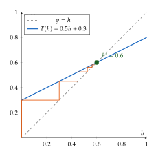
Consider the scalar recurrence $h_{t + 1} = 0.5 h_{t} + 0.3$ . The map $T (h) = 0.5 h + 0.3$ has Lipschitz constant $L = 0.5 < 1$ , so it is a contraction on $(ℝ, | \cdot |)$ . The unique fixed point satisfies $h^{*} = 0.5 h^{*} + 0.3$ , giving $h^{*} = 0.6$ . Starting from any $h_{0} \in ℝ$ , the iterates converge: $\begin{matrix} h_{0} = 0 \to h_{1} = 0.3 \to h_{2} & = 0.45 \to h_{3} = 0.525 \\ \to h_{4} & = 0.5625 \to \dots \to h^{*} = 0.6. \end{matrix}$ The error decreases geometrically from wherever it starts: $| h_{n} - 0.6 | = | h_{0} - 0.6 | \cdot {0.5}^{n}$ , which is $0.6 \cdot {0.5}^{n}$ for the run above and $0.4 \cdot {0.5}^{n}$ from $h_{0} = 1$ .

Cobweb (staircase) diagram for the recurrence

h_{t + 1} = 0.5 h_{t} + 0.3

. The orange path shows the iterates climbing in a monotone staircase from

h_{0} = 0

toward the fixed point

h^{*} = 0.6

(green dot), where the line

y = h

intersects the map

T (h) = 0.5 h + 0.3

Vanishing Gradients Revisited

The book already noted the vanishing/exploding gradient problem for vanilla RNNs (see the Remark following Definition 10). Here we make the analysis precise and show how gated architectures resolve it.

Proposition 2 (Gradient of RNN Hidden State).

For the vanilla RNN $𝒉_{t} = σ (W_{h} 𝒉_{t - 1} + W_{x} 𝒙_{t} + 𝒃)$ , the gradient of $𝒉_{T}$ with respect to $𝒉_{t}$ for $t < T$ is the matrix product (RNN Gradient Product) $\begin{matrix} \frac{\partial 𝒉_{T}}{\partial 𝒉_{t}} = \prod_{k = t + 1}^{T} diag (σ^{'} (𝒂_{k})) W_{h}, \end{matrix}$ where $𝒂_{k} = W_{h} 𝒉_{k - 1} + W_{x} 𝒙_{k} + 𝒃$ is the pre-activation at step $k$ . Consequently:

If $‖ W_{h} ‖ < 1 / \max_{z} | σ^{'} (z) |$ , then each factor has operator norm strictly less than $1$ , and the product vanishes exponentially: $‖ \partial 𝒉_{T} / \partial 𝒉_{t} ‖ \leq (‖ W_{h} ‖ \cdot \max | σ^{'} |)^{T - t} \to 0$ .
If $‖ W_{h} ‖ > 1 / \max_{z} | σ^{'} (z) |$ , gradients can explode exponentially.

Proof.

By the chain rule, $\frac{\partial 𝒉_{T}}{\partial 𝒉_{t}} = \frac{\partial 𝒉_{T}}{\partial 𝒉_{T - 1}} \cdot \frac{\partial 𝒉_{T - 1}}{\partial 𝒉_{T - 2}} \dots \frac{\partial 𝒉_{t + 1}}{\partial 𝒉_{t}} .$ Each factor is $\frac{\partial 𝒉_{k}}{\partial 𝒉_{k - 1}} = diag (σ^{'} (𝒂_{k})) W_{h}$ , yielding (RNN Gradient Product). The norm bound follows from submultiplicativity: $‖ \prod_{k} A_{k} ‖ \leq \prod_{k} ‖ A_{k} ‖$ .

∎

Proposition 3 (LSTM Gradient Highway).

The LSTM cell state (Definition 11) satisfies $𝒄_{t} = 𝒇_{t} ⊙ 𝒄_{t - 1} + 𝒊_{t} ⊙ {\tilde{𝒄}}_{t}$ . The Jacobian of the cell state is (LSTM Gradient) $\begin{matrix} \frac{\partial 𝒄_{t}}{\partial 𝒄_{t - 1}} = diag (𝒇_{t}) + (terms from gate derivatives) . \end{matrix}$ When the forget gate satisfies $𝒇_{t} \approx 1$ and the gate derivative terms are small, $\partial 𝒄_{t} / \partial 𝒄_{t - 1} \approx I$ . Over many time steps, (LSTM Gradient Product) $\begin{matrix} \frac{\partial 𝒄_{T}}{\partial 𝒄_{t}} \approx \prod_{k = t + 1}^{T} diag (𝒇_{k}), \end{matrix}$ which remains close to the identity when all forget gates are near one. This is the “gradient highway” that allows LSTMs to learn dependencies spanning hundreds of time steps.

Proof.

Differentiating the cell update $𝒄_{t} = 𝒇_{t} ⊙ 𝒄_{t - 1} + 𝒊_{t} ⊙ {\tilde{𝒄}}_{t}$ with respect to $𝒄_{t - 1}$ , we obtain $\frac{\partial 𝒄_{t}}{\partial 𝒄_{t - 1}} = diag (𝒇_{t}) + diag (𝒄_{t - 1}) \frac{\partial 𝒇_{t}}{\partial 𝒄_{t - 1}} + diag ({\tilde{𝒄}}_{t}) \frac{\partial 𝒊_{t}}{\partial 𝒄_{t - 1}} + diag (𝒊_{t}) \frac{\partial {\tilde{𝒄}}_{t}}{\partial 𝒄_{t - 1}} .$ In the LSTM, the gates $𝒇_{t}$ and $𝒊_{t}$ depend on $𝒉_{t - 1}$ , which itself depends on $𝒄_{t - 1}$ via $𝒉_{t - 1} = 𝒐_{t - 1} ⊙ \tanh (𝒄_{t - 1})$ . The three correction terms are controlled as follows.

The second term carries $\partial 𝒇_{t} / \partial 𝒄_{t - 1}$ , whose sigmoid factor evaluated at the gate's own output is $𝒇_{t} ⊙ (1 - 𝒇_{t})$ . In the copy regime $𝒇_{t} \to 1$ this is $O (‖ 1 - 𝒇_{t} ‖)$ : it vanishes at the same rate as the gate saturates. (At $𝒇_{t} = 0.99$ the factor is $0.99 \times 0.01 = 0.0099$ . The familiar bound $\max_{z} σ^{'} (z) = 1 / 4$ is attained at $𝒇_{t} = 1 / 2$ , the opposite regime, and a factor of $1 / 4$ compounded over $T - t$ steps is not small.)

The third and fourth terms are governed by the input gate $𝒊_{t}$ , which in the LSTM is a separate gate and is not tied to $𝒇_{t}$ . Forget-gate saturation alone therefore says nothing about them: the third term carries $𝒊_{t} ⊙ (1 - 𝒊_{t})$ and the fourth carries $diag (𝒊_{t})$ directly, so both are $O (‖ 𝒊_{t} ‖)$ only when the cell is additionally not writing.

Hence the honest hypothesis is $𝒇_{t} \to 1$ and $𝒊_{t} \to 0$ , under which all three corrections are $O (‖ 1 - 𝒇_{t} ‖ + ‖ 𝒊_{t} ‖)$ and the dominant contribution is $diag (𝒇_{t})$ . That is exactly the regime in which a cell is carrying information rather than overwriting it, which is the regime the gradient highway describes. The product formula (LSTM Gradient Product) then follows by induction. (In the coupled-gate variant $𝒊_{t} = 1 - 𝒇_{t}$ the second condition is implied by the first, which is one reason that variant is easier to analyse; see Exercise 5.)

∎

Exercise 1.

For a vanilla RNN with sigmoid activation $σ (z) = 1 / (1 + e^{- z})$ , show that $\max_{z} | σ^{'} (z) | = 1 / 4$ . Conclude that the gradient vanishes whenever $‖ W_{h} ‖ < 4$ . Why does this make training difficult in practice?

Connection to Dynamical Systems

The hidden-state sequence $𝒉_{0}, 𝒉_{1}, 𝒉_{2}, \dots$ produced by an RNN is the orbit of the initial condition $𝒉_{0}$ under the discrete dynamical system $𝒉_{t + 1} = F (𝒉_{t}, 𝒙_{t + 1})$ . This connection to dynamical systems theory offers rich insights:

A fixed point $𝒉^{*}$ with $F (𝒉^{*}, 𝒙) = 𝒉^{*}$ is an equilibrium. If $F (\cdot, 𝒙)$ is a contraction, the equilibrium is a globally stable attractor: all orbits converge to it (Theorem 1).
If the spectral radius of the Jacobian $\partial F / \partial 𝒉$ at $𝒉^{*}$ is less than one, the equilibrium is locally stable even if $F$ is not a global contraction.
If the spectral radius exceeds one, the system can exhibit complex behaviour, including limit cycles and chaos.

Remark 3 (Chaos in Recurrent Networks).

When the weight matrix $W_{h}$ has large spectral norm, the RNN map can become expansive rather than contractive. In this regime, small changes to the input or initialisation can lead to exponentially diverging hidden-state trajectories, the hallmark of deterministic chaos. This “edge of chaos” regime is both a curse (it causes exploding gradients) and a blessing (it allows the network to exhibit rich, input-sensitive dynamics necessary for complex computation).

Computational Limits of Transformers

We have seen that recurrence provides a mechanism for iterative computation. But the dominant architecture of modern generative modelling, the Transformer, deliberately avoids recurrence in favour of parallel self-attention. What are the consequences of this design choice for reasoning? In this section, we develop the circuit complexity framework needed to answer this question precisely.

Circuit Complexity Classes

A Boolean circuit is a directed acyclic graph whose internal nodes are logic gates (AND, OR, NOT, etc.) and whose leaves are input bits. The size of a circuit is the number of gates; the depth is the length of the longest path from an input to an output. We are interested in families of circuits ${C_{n}}_{n \geq 1}$ , one for each input length $n$ .

Definition 4 (Boolean Circuit Complexity Classes).

The following classes of circuit families are central to our discussion:

${𝖠 𝖢}^{0}$ : constant-depth, polynomial-size circuits with unbounded fan-in AND and OR gates, and NOT gates.
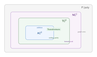
${𝖳 𝖢}^{0}$ : constant-depth, polynomial-size circuits with unbounded fan-in AND, OR and NOT gates together with threshold (majority) gates. A threshold gate outputs $1$ if and only if at least half of its inputs are $1$ . Negation is essential: without it none of these classes would contain parity, since every function computed by a monotone circuit is monotone.
${𝖭 𝖢}^{1}$ : $O (\log n)$ -depth, polynomial-size circuits with bounded fan-in AND and OR gates (each with at most $2$ inputs) and NOT gates.
$𝖯 / 𝗉 𝗈 𝗅 𝗒$ : polynomial-size circuit families (no depth restriction, not necessarily uniform).

The known inclusion chain is (Circuit Inclusions) $\begin{matrix} {𝖠 𝖢}^{0} ⊊ {𝖳 𝖢}^{0} \subseteq {𝖭 𝖢}^{1} \subseteq 𝖯 / 𝗉 𝗈 𝗅 𝗒 . \end{matrix}$ The first inclusion is strict: ${𝖠 𝖢}^{0} \neq {𝖳 𝖢}^{0}$ . The other inclusions are not known to be strict, but are widely conjectured to be so.

Example 2 (Parity is not in ${𝖠 𝖢}^{0}$ ).

The parity function $PAR (x_{1}, \dots, x_{n}) = x_{1} \oplus︎ x_{2} \oplus︎ \dots \oplus︎ x_{n}$ (the XOR of $n$ bits) lies in ${𝖳 𝖢}^{0}$ : a constant-depth, polynomial-size circuit of threshold gates computes it, for instance by forming the sum $\sum_{i} x_{i}$ with a depth-2 threshold network and reading off its low-order bit. It is worth noting that no single threshold gate can do this. A threshold gate outputs $𝟏 [\sum_{i} w_{i} x_{i} \geq t]$ and therefore computes only linearly separable functions, and parity is the textbook example of one that is not: already at $n = 2$ , XOR would require $w_{1} \geq t$ , $w_{2} \geq t$ , $t > 0$ and $w_{1} + w_{2} < t$ , which is inconsistent since $w_{1} + w_{2} \geq 2 t > t$ . However, the celebrated result of Furst, Saxe, and Sipser (1984), later sharpened by Hastad (1987), shows that any ${𝖠 𝖢}^{0}$ circuit computing parity requires exponential size: $PAR \notin {𝖠 𝖢}^{0}$ . This demonstrates that the strict inclusion ${𝖠 𝖢}^{0} ⊊ {𝖳 𝖢}^{0}$ is well established.

Caution.

Circuit complexity measures what can be computed in bounded depth. A standard Transformer with $L$ layers has depth $O (L)$ , independent of the input length $n$ , so it computes a constant-depth circuit for every input length. This is the key connection: Transformers are fundamentally bounded-depth computing devices.

Transformers as Bounded-Depth Computation

We now state the central complexity-theoretic result about Transformers.

Theorem 2 (Transformers are in ${𝖳 𝖢}^{0}$ [8]).

A Transformer with a fixed number of layers $L$ , attention heads $H$ , and embedding dimension $d$ , operating on inputs of length $n$ with $O (\log n)$ -bit precision, can be simulated by a uniform ${𝖳 𝖢}^{0}$ circuit family. Specifically, for any fixed architecture, there exists a family of threshold circuits of constant depth and polynomial size (in $n$ ) that computes the same function.

Proof sketch.

The proof proceeds layer by layer.

Attention. Each attention head computes inner products between query and key vectors (polynomial-time arithmetic, implementable in ${𝖳 𝖢}^{0}$ given $O (\log n)$ -precision), followed by a softmax (exponentiation and division, also in ${𝖳 𝖢}^{0}$ ), followed by a weighted sum of value vectors. Each of these operations can be computed by a constant-depth threshold circuit of polynomial size.

Feed-forward layers. Each position independently undergoes an affine transformation followed by an activation function (typically ReLU or GELU). These are piecewise-polynomial operations on $O (\log n)$ -bit numbers, computable in ${𝖳 𝖢}^{0}$ .

Layer normalisation. Computing the mean and variance across a vector of $d$ entries (where $d$ is a constant) is a fixed-size arithmetic operation, hence trivially in ${𝖳 𝖢}^{0}$ .

Composition. Since $L$ is a constant, composing $L$ layers of ${𝖳 𝖢}^{0}$ circuits yields a ${𝖳 𝖢}^{0}$ circuit (constant times a constant is still constant depth).

The “uniform” qualifier means that the circuit description can itself be computed in logarithmic space from $n$ , which follows from the regular structure of the Transformer architecture.

∎

Corollary 1 (Inherent Limitations of Fixed-Depth Transformers).

A fixed-depth Transformer cannot solve any problem that lies outside ${𝖳 𝖢}^{0}$ in a single forward pass. This includes problems believed to require super-constant depth, such as:

Boolean formula evaluation: evaluating an arbitrary Boolean formula on given inputs (complete for ${𝖭 𝖢}^{1}$ ).
Graph connectivity: determining whether two nodes in a graph are connected (in $𝖭 𝖫 \subseteq {𝖭 𝖢}^{2}$ ).
Iterated matrix product: computing the product of $n$ matrices of constant dimension (complete for ${𝖦 𝖺 𝗉 𝖭 𝖢}^{1}$ ). Note the contrast with iterated multiplication of $n$ integers, which is in DLOGTIME-uniform ${𝖳 𝖢}^{0}$ , along with integer division and powering (Hesse, 2001).

Insight.

This result does not mean that Transformers are weak. ${𝖳 𝖢}^{0}$ is a powerful class that includes integer multiplication, sorting, and many practical tasks. But it does mean there are mathematical limits to what a single forward pass can compute, regardless of model size. Scaling up parameters (making the circuit wider) does not help; the depth constraint is the binding one.

The circuit complexity hierarchy. Transformers with a fixed number of layers compute functions in

{𝖳 𝖢}^{0}

(green region). Parity and sorting sit inside

{𝖳 𝖢}^{0}

but outside

{𝖠 𝖢}^{0}

, which is why they are drawn in the annulus between the two. Only the separation

{𝖠 𝖢}^{0} ⊊ {𝖳 𝖢}^{0}

drawn here is proved. The placements of Boolean formula evaluation outside

{𝖳 𝖢}^{0}

and of graph connectivity outside

{𝖭 𝖢}^{1}

rest on the widely believed but still open separations

{𝖳 𝖢}^{0} \neq {𝖭 𝖢}^{1}

and

{𝖭 𝖢}^{1} \neq 𝖭 𝖫

; under those conjectures, neither can be solved in a single forward pass, no matter how large the model.

Chain-of-Thought Reasoning

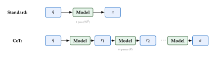
The central lesson of Computational Limits of Transformers is stark: a single forward pass through a fixed-depth Transformer is limited to ${𝖳 𝖢}^{0}$ . But what if the model is allowed to perform multiple forward passes, writing intermediate results to a “scratchpad” that it can read back on subsequent passes? This simple idea, generating intermediate tokens before the final answer, turns out to fundamentally change the computational power of the model.

Scratchpads and Intermediate Computation

The idea of augmenting a neural network with a scratchpad for intermediate computation was explored by Nye et al. [23], who trained Transformers to solve multi-step arithmetic problems. Rather than mapping directly from input to output, the model was trained to produce the full sequence of intermediate computation steps (carries, partial sums, etc.) before writing the final answer.

Definition 5 (Scratchpad Augmentation).

Given an input $𝒙$ , a scratchpad-augmented model generates a sequence of intermediate tokens $𝒔 = (s_{1}, s_{2}, \dots, s_{K})$ before producing the final output $𝒚$ . The joint distribution factorises as (Scratchpad) $\begin{matrix} p (𝒚 | 𝒙) = \sum_{𝒔} p (𝒚 | 𝒔, 𝒙) p (𝒔 | 𝒙), \end{matrix}$ where $𝒔$ ranges over all possible scratchpad sequences of length up to $K$ . In practice, since the sum is intractable, the model generates a single scratchpad sequence autoregressively and conditions the answer on it.

The critical observation is that each token generation is a separate forward pass. If the model generates $K$ intermediate tokens, it effectively performs $K + 1$ sequential forward passes, each of which is a ${𝖳 𝖢}^{0}$ computation that can read the results of all previous passes. This sequential composition is far more powerful than a single pass.

Chain-of-Thought Prompting

The scratchpad idea was implicit in the training procedure of Nye et al. Wei et al. [5] made it explicit at inference time through chain-of-thought (CoT) prompting: by including step-by-step reasoning exemplars in the prompt, they showed that large language models could be induced to generate intermediate reasoning steps for novel problems.

Definition 6 (Chain-of-Thought Prompting).

Given a question $q$ , chain-of-thought prompting [5] induces the model to generate a reasoning chain $𝒓 = (r_{1}, r_{2}, \dots, r_{m})$ of intermediate tokens followed by a final answer $a$ . The model's probability of the correct answer factorises as (COT) $\begin{matrix} p (a | q) = \sum_{𝒓} p (a | 𝒓, q) \cdot p (𝒓 | q), \end{matrix}$ where $𝒓$ ranges over all possible reasoning chains. In practice, the model generates a single chain autoregressively: (COT Autoregressive) $\begin{matrix} p (𝒓, a | q) = p (r_{1} | q) p (r_{2} | r_{1}, q) \dots p (r_{m} | r_{1 : m - 1}, q) p (a | 𝒓, q) . \end{matrix}$

Remarkably, Kojima et al. [24] showed that the simple prompt suffix “Let's think step by step” is sufficient to elicit chain-of-thought reasoning in large language models, even without any exemplars. This is known as zero-shot CoT.

Example 3 (Standard vs. Chain-of-Thought Prompting).

Consider the arithmetic word problem:

Q: Roger has 5 tennis balls. He buys 2 more cans of 3 tennis balls each. How many tennis balls does he have now?

Standard prompting: A: 11.

Chain-of-thought prompting: A: Roger started with 5 balls. He bought 2 cans of 3 balls each, so he bought $2 \times 3 = 6$ balls. Now he has $5 + 6 = 11$ balls. The answer is $11$ .

In the CoT version, every token of the worked solution is a separate forward pass, so the two intermediate results ( $2 \times 3 = 6$ , then $5 + 6 = 11$ ) cost as many passes as they take tokens to write, and each pass can condition on everything written before it. The steps are the useful unit for a reader; the tokens are the unit of computation, and it is the token count that buys the sequential depth.

Theoretical Foundations: The Power of Intermediate Steps

We now present the theoretical results that explain why chain-of-thought is so powerful. The key insight is that CoT changes the model's computational class.

Theorem 3 (Impossibility Without CoT [9]).

Assume ${𝖳 𝖢}^{0} \neq {𝖭 𝖢}^{1}$ . Then there are problems solvable in polynomial time that no fixed-depth Transformer solves in a single forward pass at logarithmic precision. More precisely: for any Transformer with a fixed number of layers $L$ , fixed number of heads $H$ , fixed embedding dimension $d$ , and $O (\log n)$ -bit precision, there exists a function $f \in 𝖯$ (indeed $f \in {𝖭 𝖢}^{1}$ ) and infinitely many input lengths $n$ at which the Transformer fails to compute $f$ correctly on at least one input of length $n$ .

Proof sketch.

By Theorem 2, any fixed-depth log-precision Transformer computes a function in uniform ${𝖳 𝖢}^{0}$ . Take $f$ to be iterated composition of permutations on five elements, which is ${𝖭 𝖢}^{1}$ -complete under ${𝖠 𝖢}^{0}$ reductions (Barrington's theorem). If a fixed-depth Transformer computed $f$ on all inputs of every sufficiently large length, then ${𝖭 𝖢}^{1} \subseteq {𝖳 𝖢}^{0}$ , and with the inclusion ${𝖳 𝖢}^{0} \subseteq {𝖭 𝖢}^{1}$ from Definition 4 the two classes would coincide, contradicting the hypothesis.

∎

Remark 4.

The conditional form is not a technicality to be waved away: no unconditional separation of uniform ${𝖳 𝖢}^{0}$ from $𝖯$ is known, and proving one would be a major result in complexity theory. Definition 4 already records that ${𝖳 𝖢}^{0} \subseteq {𝖭 𝖢}^{1}$ is not known to be strict, and the theorem above is exactly the statement that becomes available once it is. What the theorem does deliver unconditionally is the shape of the argument: a bounded-depth device cannot escape its own circuit class, so any escape must come from outside the forward pass. That is what the next section supplies.

This impossibility result motivates chain-of-thought: if a single pass is insufficient, perhaps multiple passes suffice?

Theorem 4 (Sufficiency of CoT [10]).

A polynomial-size autoregressive Transformer with chain-of-thought, that is, allowed to generate polynomially many intermediate tokens before producing the final answer, can solve any problem in $𝖯$ . Formally: for any language $ℒ \in 𝖯$ , there exists a constant-depth Transformer $T$ and a polynomial $p (n)$ such that, given input $𝒙$ of length $n$ , the Transformer generates at most $p (n)$ intermediate tokens and then outputs the correct answer (accept/reject) for $ℒ$ .

Proof sketch.

The proof constructs a Transformer that simulates a Turing machine. The key steps are:

Encoding. The scratchpad at each step encodes the current configuration of a Turing machine (tape contents, head position, state).
One-step simulation. A single forward pass of the Transformer reads the current configuration and writes the next configuration. This requires reading the symbol under the head, looking up the transition function, and updating the tape, head, and state. Each of these operations is a bounded look-up, which is computable in ${𝖳 𝖢}^{0}$ (in fact, even in ${𝖠 𝖢}^{0}$ , since the transition table is constant-size).
Iteration. By generating $p (n)$ intermediate tokens (one per Turing machine step), the Transformer simulates $p (n)$ steps of the Turing machine. Since $ℒ \in 𝖯$ , there exists a polynomial-time Turing machine deciding $ℒ$ , and $p (n)$ steps suffice.

The construction yields a Transformer with a number of layers, heads, and embedding dimension that depend on the Turing machine (but not on $n$ ), and a scratchpad of length at most $p (n)$ .

∎

Corollary 2 (From ${𝖳 𝖢}^{0}$ to $𝖯$ with Chain-of-Thought).

A single forward pass of a fixed-depth, $O (\log n)$ -precision Transformer computes a function in uniform ${𝖳 𝖢}^{0}$ , and the same Transformer allowed a polynomial-length chain of thought decides every language in $𝖯$ . If, as is widely believed, ${𝖳 𝖢}^{0} ⊊ 𝖯$ , then chain-of-thought strictly enlarges what the model can compute.

Remark 5.

Both halves of the corollary are unconditional; only the word “strictly” is not. Since uniform ${𝖳 𝖢}^{0} \subseteq {𝖭 𝖢}^{1} \subseteq 𝖫 \subseteq 𝖯$ , a collapse ${𝖳 𝖢}^{0} = 𝖯$ would force $𝖫 = 𝖯$ as well, which is open. Nobody expects that, but it has not been ruled out, and the honest statement is worth keeping in view: what is proved is the pair of containments, not the gap between them.

Key Idea.

Chain-of-thought is not merely a prompting trick; it changes the computational class the model can reach. A single forward pass computes a function in ${𝖳 𝖢}^{0}$ ; a polynomial chain of forward passes computes any function in $𝖯$ . The intermediate tokens serve as the working memory that a bounded-depth circuit otherwise lacks.

Standard prompting (top) uses a single forward pass, computing a

{𝖳 𝖢}^{0}

function. Chain-of-thought (bottom) uses

m

sequential forward passes, with each intermediate token

r_{i}

serving as working memory. This elevates the computational class to

𝖯

Self-Consistency

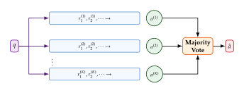
A single chain of thought may contain errors. Wang et al. [25] proposed self-consistency decoding, which samples multiple reasoning chains and takes a majority vote over the final answers.

Definition 7 (Self-Consistency Decoding).

Given a question $q$ , self-consistency decoding proceeds as follows:

Sample $K$ independent reasoning chains $𝒓^{(1)}, 𝒓^{(2)}, \dots, 𝒓^{(K)} \sim p (𝒓 | q)$ .
Extract the final answer from each chain: $a^{(k)} = extract (𝒓^{(k)})$ for $k = 1, \dots, K$ .
Return the majority vote: (SELF Consistency) $\begin{matrix} \hat{a} = {arg max}_{a} \sum_{k = 1}^{K} 𝟏 [a^{(k)} = a] . \end{matrix}$

The following proposition makes precise the sense in which self-consistency reduces errors.

Proposition 4 (Error Reduction via Self-Consistency).

Suppose the model produces the correct answer $a^{*}$ for a binary question independently with probability $p > 1 / 2$ on each sampled chain. Then the probability that the majority vote over $K$ chains yields the correct answer satisfies (SELF Consistency Bound) $\begin{matrix} P (majority correct) \geq 1 - \exp (- 2 K (p - \frac{1}{2})^{2}), \end{matrix}$ which converges exponentially fast to $1$ as $K \to \infty$ .

Proof.

Let $S = \sum_{k = 1}^{K} 𝟏 [a^{(k)} = a^{*}]$ be the number of correct answers among the $K$ chains. The majority vote is correct if and only if $S > K / 2$ . Since each chain is independent with $𝔼 [𝟏 [a^{(k)} = a^{*}]] = p$ , we have $𝔼 [S] = K p$ . By the Hoeffding bound applied to the random variables $X_{k} = 𝟏 [a^{(k)} = a^{*}] \in [0,1]$ , $\begin{matrix} P (S \leq K / 2) & = P (S - K p \leq K / 2 - K p) = P (S - K p \leq - K (p - \frac{1}{2})) \\ \leq \exp (- 2 K (p - \frac{1}{2})^{2}), \end{matrix}$ where we used the Hoeffding inequality $P (\overline{X} - μ \leq - t) \leq \exp (- 2 K t^{2})$ with $t = p - 1 / 2 > 0$ . Therefore, $P (majority correct) = P (S > K / 2) \geq 1 - \exp (- 2 K {(p - 1 / 2)}^{2})$ .

∎

Self-consistency decoding.

K

independent reasoning chains are sampled from the model, each producing an answer. The final answer

\hat{a}

is the majority vote. By Proposition 4, the error probability decreases exponentially in

K

Tree of Thoughts

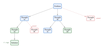
Chain-of-thought generates a single linear chain of reasoning steps. But many problems have a combinatorial structure that is better explored with tree search: at each step, multiple continuations are possible, and some may lead to dead ends. Yao et al. [11] proposed Tree of Thoughts (ToT), which organises the reasoning process as a search over a tree.

Definition 8 (Tree of Thoughts (ToT)).

The Tree of Thoughts framework [11] organises reasoning as a search over a tree $𝒯$ where:

Each node represents a partial reasoning state $s$ (a prefix of a reasoning chain).
The children of $s$ are generated by prompting the language model to propose $b$ “next thoughts,” candidate continuations of the reasoning chain.
A value function $V (s)$ , implemented by prompting the same language model, evaluates how promising each partial state is (e.g., “sure/maybe/impossible”).
A search algorithm (breadth-first search or depth-first search) explores the tree, using $V (s)$ to prioritise or prune branches.

Algorithm 1 (Tree of Thoughts – BFS Variant).

Input: Problem $q$ ; branching factor $b$ ; beam width $w$ ; maximum depth $D$ ; LM-based thought generator $G$ and evaluator $V$ . Output: Best reasoning chain $𝒓^{*}$ .

Initialise the frontier $𝒮_{0} \leftarrow {s_{0}}$ where $s_{0}$ encodes the problem $q$ .
For depth $d = 1, \dots, D$ : enumerate
Expand: For each $s \in 𝒮_{d - 1}$ , generate $b$ candidate next thoughts using $G$ : ${t_{1}, \dots, t_{b}} \sim G (\cdot | s)$ .
Evaluate: For each candidate $s^{'} = (s, t_{j})$ , compute $V (s^{'})$ .
Select: Keep the top- $w$ states by value: $𝒮_{d} \leftarrow top - w ({(s, t_{j}) : s \in 𝒮_{d - 1}, j = 1, \dots, b})$ . enumerate
Return $𝒓^{*} = {arg max}_{s \in 𝒮_{D}} V (s)$ .

Remark 6 (CoT vs. ToT: Depth vs. Breadth).

Standard CoT explores a single path through the reasoning space. Self-consistency samples multiple independent paths (no interaction between them). ToT explores a tree, where the evaluation at each node can guide the search toward more promising regions. This is analogous to the distinction between greedy search, random restarts, and beam search in classical optimisation. The cost is higher: ToT requires $O (b \cdot w \cdot D)$ forward passes compared to $O (m)$ for a single CoT chain of length $m$ .

Tree of Thoughts. The problem is the root; each node is a partial reasoning state. The model generates candidate “thoughts” (children) and evaluates them with a value function

V

. Low-value branches (dashed red) are pruned. The search follows the most promising path to a solution.

Reinforcement Learning for Reasoning

Chain-of-thought provides the mechanism for multi-step reasoning, but where do the reasoning chains come from? The approaches in Chain-of-Thought Reasoning relied on either human-written demonstrations (few-shot CoT) or the model's pre-existing ability (zero-shot CoT). A natural question is: can models discover effective reasoning strategies on their own, through trial and error? This is the domain of reinforcement learning (RL), and its application to reasoning has produced some of the most striking results in recent AI research.

From Supervised CoT to Self-Discovery

The bridge between supervised chain-of-thought and RL-based discovery is the Self-Taught Reasoner (STaR) algorithm of Zelikman et al. [26]. The key idea is to bootstrap reasoning ability from a small set of examples by iteratively generating, filtering, and learning from the model's own reasoning chains.

Algorithm 2 (Self-Taught Reasoner (STaR)).

Input: Dataset $𝒟 = {(q_{i}, a_{i})}_{i = 1}^{N}$ of question–answer pairs; a few seed CoT demonstrations; initial model $π_{θ}$ . Output: Improved model $π_{θ^{*}}$ .

Generate: For each question $q_{i} \in 𝒟$ , sample a reasoning chain $𝒓_{i} \sim π_{θ} (\cdot | q_{i})$ and extract the predicted answer ${\hat{a}}_{i}$ .
Filter: Keep only chains that produced the correct answer: $𝒟_{correct} = {(q_{i}, 𝒓_{i}, a_{i}) : {\hat{a}}_{i} = a_{i}}$ .
Rationalise: For questions where the model failed, provide the correct answer as a hint and generate a new chain conditioned on it. Add successful rationalisations to $𝒟_{correct}$ .
Fine-tune: Update $θ$ by supervised fine-tuning on $𝒟_{correct}$ (maximise $\sum \log π_{θ} (𝒓_{i}, a_{i} | q_{i})$ ).
Iterate: Return to Step 1 with the updated model. Repeat until convergence.

Remark 7 (STaR as Approximate RL).

STaR can be viewed as a simplified form of policy gradient RL. The “reward” is binary (correct or incorrect answer), and the policy update (Step 4) plays the role of a REINFORCE update with a reward of $1$ for correct chains and $0$ for incorrect ones, except that it uses the maximum-likelihood objective rather than the policy gradient estimator. The correspondence is exact only for the filtered on-policy chains: $𝒟_{correct}$ also holds the rationalised chains from Step 3, which were sampled from $π_{𝜽} (\cdot | q_{i}, a_{i})$ with the answer in hand and are carried with no importance weight, so they are off-policy. That step (Step 3) is a form of hindsight experience replay.

Policy Optimisation Background

To understand the more sophisticated RL methods used for reasoning, we need the basic tools of policy optimisation. We present them here in the context of language generation, where the “environment” is the problem to be solved and the “trajectory” is the generated reasoning chain.

Definition 9 (REINFORCE Estimator).

Let $π_{θ}$ be a policy (language model) parameterised by $𝜽$ that generates a trajectory (token sequence) $τ = (t_{1}, t_{2}, \dots, t_{M})$ with probability $π_{θ} (τ) = \prod_{m = 1}^{M} π_{θ} (t_{m} | t_{1 : m - 1})$ . Let $R (τ)$ be a scalar reward for the complete trajectory. The REINFORCE estimator [12] of the policy gradient is (Reinforce) $\begin{matrix} \nabla_{𝜽} J (𝜽) = 𝔼_{τ \sim π_{𝜽}} [R (τ) \nabla_{𝜽} \log π_{𝜽} (τ)], \end{matrix}$ which can be estimated by sampling trajectories $τ^{(1)}, \dots, τ^{(K)} \sim π_{𝜽}$ and computing (Reinforce Estimator) $\begin{matrix} {\hat{\nabla}}_{𝜽} J (𝜽) = \frac{1}{K} \sum_{k = 1}^{K} R (τ^{(k)}) \nabla_{𝜽} \log π_{𝜽} (τ^{(k)}) . \end{matrix}$

Remark 8 (Variance Reduction).

The REINFORCE estimator has notoriously high variance. A standard remedy is to subtract a baseline $b$ from the reward: replace $R (τ)$ by $R (τ) - b$ in (Reinforce). Provided $b$ does not depend on the sampled trajectory $τ$ , this leaves the expected gradient unchanged: (Baseline Unbiased) $\begin{matrix} 𝔼_{τ} [b \nabla_{𝜽} \log π_{𝜽} (τ)] = b \sum_{τ} π_{𝜽} (τ) \frac{\nabla_{𝜽} π_{𝜽} (τ)}{π_{𝜽} (τ)} = b \sum_{τ} \nabla_{𝜽} π_{𝜽} (τ) = b \nabla_{𝜽} \sum_{τ} π_{𝜽} (τ) = b \nabla_{𝜽} 1 = 0, \end{matrix}$ while the variance can drop dramatically. The independence hypothesis is the load-bearing one, and it is worth marking now: a baseline computed from the same samples it is applied to does not satisfy it, which is exactly the situation in Proposition 5. Common baselines that do satisfy it include a running mean of rewards over past questions and a learned value function $V (s)$ .

Definition 10 (Proximal Policy Optimisation (PPO)).

PPO [13] prevents destructively large policy updates by clipping the importance sampling ratio. Let $ρ_{t} (𝜽) = π_{𝜽} (a_{t} | s_{t}) / π_{𝜽_{old}} (a_{t} | s_{t})$ be the ratio of the new policy to the old policy for action $a_{t}$ in state $s_{t}$ . The PPO-Clip objective is (PPO) $\begin{matrix} L^{CLIP} (𝜽) = 𝔼 [\min (ρ_{t} (𝜽) {\hat{A}}_{t}, clip (ρ_{t} (𝜽), 1 - ϵ, 1 + ϵ) {\hat{A}}_{t})], \end{matrix}$ where ${\hat{A}}_{t}$ is the estimated advantage (how much better action $a_{t}$ is compared to the baseline), and $ϵ > 0$ (typically $0.1$ – $0.2$ ) is the clipping threshold.

The clipping mechanism in (PPO) works as follows: if an action is better than expected ( ${\hat{A}}_{t} > 0$ ), the objective increases with $ρ_{t}$ but is capped at $(1 + ϵ) {\hat{A}}_{t}$ , preventing the new policy from becoming too different from the old one. Conversely, if ${\hat{A}}_{t} < 0$ , the objective does not allow $ρ_{t}$ to decrease below $1 - ϵ$ . This creates a “trust region” around the old policy.

Group Relative Policy Optimisation (GRPO)

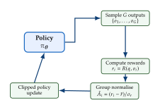
The methods above (REINFORCE, PPO) require either high-variance gradient estimates or a learned value function (critic) to compute advantages. Training a value function on long reasoning chains is itself a difficult problem: the state space is enormous (the space of all partial token sequences), and the reward is sparse (typically only available at the end of the chain). Group Relative Policy Optimisation (GRPO), introduced in the DeepSeek-Math [27] and DeepSeek-R1 [6] papers, solves this problem elegantly by eliminating the critic entirely.

Definition 11 (Group Relative Policy Optimisation (GRPO)).

Given a question $q$ , GRPO samples a group of $G$ outputs ${o_{1}, o_{2}, \dots, o_{G}}$ from the current policy: $o_{i} \sim π_{𝜽_{old}} (\cdot | q)$ . The reward for each output is $r_{i} = R (q, o_{i})$ . The advantages are estimated by group normalisation: (GRPO Advantage) $\begin{matrix} {\hat{A}}_{i} = \frac{r_{i} - mean ({r_{j}}_{j = 1}^{G})}{std ({r_{j}}_{j = 1}^{G})}, \end{matrix}$ where $mean$ and $std$ are computed over the group, with $std$ taken as the population standard deviation over the $G$ samples. (The choice matters at small $G$ : for the group ${1,1,0,1,0,0,1,0}$ the population value $0.5$ gives advantages of exactly $\pm 1$ , while the sample value $\sqrt{2 / 7} = 0.5345$ gives $\pm 0.9354$ .) When every reward in the group is equal the denominator is zero and the group contributes no gradient. The policy is updated by maximising (GRPO Objective) $\begin{matrix} J_{GRPO} (𝜽) = 𝔼_{q} [\frac{1}{G} \sum_{i = 1}^{G} \min (ρ_{i} (𝜽) {\hat{A}}_{i}, clip (ρ_{i} (𝜽), 1 - ϵ, 1 + ϵ) {\hat{A}}_{i}) - β 𝖣 (π_{𝜽} ‖ π_{ref})], \end{matrix}$ where $ϵ$ is the clipping threshold, $β > 0$ is a KL penalty coefficient, and $π_{ref}$ is a reference policy (typically the initial supervised fine-tuned model). The importance ratio is taken per token and averaged over the output, exactly as in (PPO): (GRPO Ratio) $\begin{matrix} ρ_{i} (𝜽) {\hat{A}}_{i} ⟶ \frac{1}{| o_{i} |} \sum_{t = 1}^{| o_{i} |} \min (ρ_{i, t} (𝜽) {\hat{A}}_{i}, clip (ρ_{i, t} (𝜽), 1 - ϵ, 1 + ϵ) {\hat{A}}_{i}), ρ_{i, t} (𝜽) = \frac{π_{𝜽} (o_{i, t} | q, o_{i, < t})}{π_{𝜽_{old}} (o_{i, t} | q, o_{i, < t})}, \end{matrix}$ with the same advantage ${\hat{A}}_{i}$ shared by every token of output $o_{i}$ . Clipping at the sequence level would be vacuous: a whole-sequence ratio is a product of hundreds of per-token ratios, and it leaves $[1 - ϵ, 1 + ϵ]$ after a single token moves slightly.

Key Idea.

GRPO eliminates the need for a separate value/critic network (which PPO requires). Instead, it estimates the baseline from the group statistics, a form of self-referential normalisation. This is especially important for reasoning tasks: training a value function on long reasoning chains with sparse, delayed rewards is extremely difficult. GRPO sidesteps this problem entirely by comparing each output only to its siblings in the same group.

Remark 9 (GRPO vs. PPO).

Both GRPO and PPO use clipped importance ratios to stabilise training. The critical difference is in how they compute the advantage:

PPO uses a learned value function $V_{ϕ} (s)$ to compute the advantage: ${\hat{A}}_{t} = R_{t} - V_{ϕ} (s_{t})$ , where $V_{ϕ}$ is trained by regression on observed returns. This requires maintaining and training a second network of comparable size to the policy.
GRPO uses the group mean reward as the baseline: ${\hat{A}}_{i} = (r_{i} - \overline{r}) / σ_{r}$ . No additional network is needed. The cost is that $G$ outputs must be sampled per question, but this is naturally parallelisable on modern hardware.

For large language models with billions of parameters, eliminating the critic saves substantial compute and memory.

Proposition 5 (Zero-Sum Property of the GRPO Advantage).

The group-normalised advantage ${\hat{A}}_{i}$ defined in (GRPO Advantage) satisfies, for any fixed question $q$ , $\sum_{i = 1}^{G} {\hat{A}}_{i} = 0$ . The group mean therefore acts as a baseline: outputs scoring above the group average push the policy toward themselves and outputs scoring below it push away, at a scale set by the spread within the group rather than by the absolute scale of rewards.

Proof.

By definition, $\sum_{i = 1}^{G} {\hat{A}}_{i} = \sum_{i = 1}^{G} \frac{r_{i} - \overline{r}}{σ_{r}} = \frac{1}{σ_{r}} (\sum_{i = 1}^{G} r_{i} - G \overline{r}) = \frac{1}{σ_{r}} (G \overline{r} - G \overline{r}) = 0$ .

∎

Caution.

The estimator is not unbiased. Zero-sum is not the same as unbiased, and GRPO's gradient estimator is not unbiased. The baseline argument of Definition 9 needs $𝔼 [b \nabla \log π_{θ}] = b \nabla 1 = 0$ , which requires $b$ to be independent of the sampled action. The group mean $\overline{r}$ is computed from $o_{1}, \dots, o_{G}$ including $o_{i}$ itself, so that independence fails; the division by the sample standard deviation $σ_{r}$ , also computed from the same samples, adds a second source of bias, and is undefined when every reward in the group is equal. Several later variants drop the $σ_{r}$ division for exactly this reason. In practice the bias is small at moderate $G$ and is accepted in exchange for removing the critic network entirely.

The GRPO training loop. From the current policy,

G

outputs are sampled for each question. Rewards are computed (typically by rule-based verification) and normalised within the group to form advantages. A clipped policy update then adjusts the model. No separate critic network is needed.

DeepSeek-R1: A Case Study

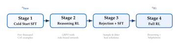
The DeepSeek-R1 model [6] provides a compelling case study of how reinforcement learning can elicit sophisticated reasoning behaviour from a large language model. Its training pipeline comprises four stages, each building on the previous.

Algorithm 3 (DeepSeek-R1 Training Pipeline).

Input: Base language model $π_{base}$ ; question–answer datasets for mathematics, coding, and science; rule-based reward functions. Output: Reasoning-capable model $π_{R1}$ .

Stage 1: Cold Start. Fine-tune $π_{base}$ on a small, curated dataset of high-quality chain-of-thought examples (thousands of examples, not millions). This “cold start” provides the model with the basic format of step-by-step reasoning, yielding $π_{cold}$ .

Stage 2: Reasoning RL. Apply GRPO (Definition 11) to $π_{cold}$ using rule-based rewards:

Accuracy reward: $+ 1$ for correct final answer, $0$ otherwise. For mathematics, this is exact-match comparison after normalisation. For coding, this is determined by executing the generated code against test cases.
Format reward: small bonus for placing the reasoning inside designated $⟨ 𝚝𝚑𝚒𝚗𝚔 ⟩ \dots ⟨ / 𝚝𝚑𝚒𝚗𝚔 ⟩$ tags and the answer inside $⟨ 𝚊𝚗𝚜𝚠𝚎𝚛 ⟩ \dots ⟨ / 𝚊𝚗𝚜𝚠𝚎𝚛 ⟩$ tags.

This stage runs for thousands of RL steps, progressively increasing the model's reasoning capability.

Stage 3: Rejection Sampling and SFT. Use the RL-trained model to generate many candidate solutions for each question. Filter for correct solutions and select the highest-quality ones (by length, clarity, and diversity). Perform supervised fine-tuning (SFT) on this curated dataset, yielding a model that combines the reasoning ability from RL with the fluency and format of SFT.

Stage 4: Full RL. Apply a second round of GRPO with an expanded reward signal that includes both reasoning accuracy and general helpfulness, harmlessness, and format adherence. This final stage aligns the model with broader user preferences while preserving reasoning capability.

Historical Note.

Before the four-stage pipeline above, DeepSeek trained DeepSeek-R1-Zero: the base model with reinforcement learning applied directly, and no supervised fine-tuning of any kind. It is in that run that researchers observed the phenomenon they termed the “aha moment.” After several hundred RL steps, the model spontaneously began re-examining its reasoning when it encountered inconsistencies, generating phrases like “Wait, let me reconsider” and “Hmm, I think I made an error above. Let me try again.” The absence of any supervised stage is precisely what makes this striking: no example of self-correction existed anywhere in that pipeline. The RL objective rewarded correct final answers, and the model discovered on its own that pausing to check and revise its work increased the probability of arriving at one.

R1-Zero's weakness was readability, with mixed languages and unstructured output, and that is what motivated the cold-start supervised stage of the full R1 pipeline. The reasoning behaviour itself was not taught there; it was inherited.

Remark 10 (Rule-Based vs. Learned Rewards).

A distinguishing feature of the DeepSeek-R1 approach is its reliance on rule-based rewards rather than a learned reward model. For mathematics, correctness is determined by exact-match comparison of the final numerical answer. For coding, correctness is determined by executing the generated code against a test suite. This design choice avoids the well-known problem of reward hacking, where the model exploits weaknesses in a learned reward model rather than genuinely improving its reasoning. The downside is that rule-based rewards are only available for domains with verifiable answers (math, code, formal logic), not for open-ended reasoning tasks. This is why the reliance is partial rather than total: Stage 2 is driven entirely by rules, while Stage 4 brings in preference reward models for the general, non-verifiable data, where no rule exists to check against.

The four-stage DeepSeek-R1 training pipeline. The base model is first given a “cold start” with a small number of CoT examples, then trained with GRPO on reasoning tasks, then refined with rejection sampling, and finally aligned with a broader RL objective. The shading darkens to indicate increasing capability.

Exercise 2.

(a) Show that GRPO degenerates at group size $G = 1$ : substituting $G = 1$ into , the group mean is the single sample itself, so the numerator $r_{1} - \overline{r}$ is identically zero and the update vanishes before the undefined $σ_{r}$ is even reached. (b) Now replace the group statistics by a running mean of rewards maintained across questions. Show that with no clipping this recovers the REINFORCE estimator with a moving-average baseline, and explain why that baseline is legitimate while the group mean is not: the running mean is independent of the sample it is applied to, which is exactly the hypothesis the baseline argument of Definition 9 needs.

Exercise 3.

Suppose a fixed-depth Transformer with $L$ layers attempts to solve the problem of composing $n$ permutations on ${1, \dots, 5}$ . Assuming ${𝖳 𝖢}^{0} \neq {𝖭 𝖢}^{1}$ and using Theorem 2, argue that a single forward pass cannot solve this problem for all sufficiently large $n$ . Identify precisely where the assumption is used. Then show that a chain-of-thought approach, generating $O (n)$ intermediate tokens, can solve it by composing permutations one at a time.

The “aha moment” observed during the pure-RL training of DeepSeek-R1-Zero, the run that preceded the pipeline of Algorithm 3, hinted at a striking capability: large language models can learn to recognise their own mistakes and correct them. In this section we formalise self-reflection as a species of iterative refinement and connect it, once again, to the fixed-point theory that recurs throughout this chapter. The core message is simple: if we view a model's output as a point in some space of solutions, then self-correction is nothing more than applying an operator repeatedly until we reach a fixed point.

Reflexion

Definition 12 (Reflexion).

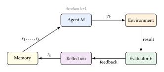
Reflexion [14] is an agent framework in which experience is stored as verbal feedback rather than gradient updates. Given a task with input $x$ , the agent proceeds as follows:

Attempt. Produce an initial output $y_{0} = M (x)$ .
Evaluate. An evaluator $E$ (which may be the model itself, a unit-test harness, or an external reward signal) scores the current attempt $y_{k}$ , starting at $k = 0$ .
Reflect. If the evaluation fails, the agent generates a natural-language reflection on that attempt, $r_{k + 1} = M (“What went wrong with y_{k} ?”)$ , summarising the failure mode.
Retry. The reflection is appended to a persistent memory buffer, which now holds $r_{1}, \dots, r_{k + 1}$ , and the task is re-attempted with the whole buffer in context: $y_{k + 1} = M (x, r_{1}, r_{2}, \dots, r_{k + 1}) .$
Increment $k$ and repeat from step 2 until $E (y_{k})$ passes or a budget is exhausted. Note that each pass reflects on the latest attempt, so the buffer grows by one reflection per round; the weights never change, only the context does.

Remark 11 (Verbal Reinforcement Learning).

Reflexion can be understood as “verbal reinforcement learning”: rather than updating model weights in response to reward, the agent updates a textual memory. The reflections play the role of a value function: they encode information about which strategies failed and why, guiding future attempts away from repeated mistakes.

The Reflexion loop. The agent attempts a task, the evaluator judges the result, and a verbal reflection is stored in memory. On the next attempt the accumulated reflections guide the agent toward success.

Self-Refine

Reflexion relies on an external evaluator. Self-Refine [28] closes the loop entirely: the same language model serves as generator, critic, and refiner.

Definition 13 (Self-Refine).

Given an input $x$ and a language model $M$ , the Self-Refine procedure iterates between three roles:

Generate. $y_{0} = M (x)$ .
Critique. $f_{k} = M (“Critique: ” ‖ y_{k})$ .
Refine. $y_{k + 1} = M (x, y_{k}, f_{k})$ .

The process terminates when the critique is vacuous (“no further improvements needed”) or when a maximum number of iterations is reached.

Let us cast this in the language of fixed-point iteration. Define the refine–critique operator (SELF Refine Operator) $\begin{matrix} T (y) ≔ Refine (x, y, Critique (y)) . \end{matrix}$ The Self-Refine loop is then simply $y_{k + 1} = T (y_{k})$ . Convergence occurs when $T (y^{⋆}) = y^{⋆}$ : the critique finds nothing to improve and the refiner reproduces the input unchanged.

Proposition 6 (Self-Refine as Fixed-Point Iteration).

Suppose the combined refine–critique operator $T$ of (SELF Refine Operator) is a contraction mapping on a complete metric space $(S, d)$ of outputs with Lipschitz constant $L < 1$ : $d (T (y), T (y^{'})) \leq L d (y, y^{'}) \forall y, y^{'} \in S .$ Then by Theorem 1 (Banach Contraction Mapping Theorem):

There exists a unique fixed point $y^{⋆} = T (y^{⋆})$ .
For any initialisation $y_{0}$ , the iterates $y_{k} = T^{k} (y_{0})$ satisfy both $d (y_{k}, y^{⋆}) \leq \frac{L^{k}}{1 - L} d (y_{1}, y_{0}) and d (y_{k}, y^{⋆}) \leq L^{k} d (y_{0}, y^{⋆}),$ i.e. convergence is geometric with rate $L$ . The first bound is computable from the first step actually taken; the second, immediate from contractivity applied $k$ times to the pair $(y_{0}, y^{⋆})$ , is the one to use when the distance to the answer is what is known.

Proof.

This is a direct application of Theorem 1. Two hypotheses have to be checked rather than assumed. First, $T$ must map $S$ into itself, which holds by construction since $Refine$ and $Critique$ both produce elements of $S$ . Second, $(S, d)$ must be complete, so that the Cauchy sequence of iterates has a limit in $S$ ; for the discrete and integer-valued metrics on text used in practice this is automatic, but for a metric on a continuous embedding space it is a real condition. The contraction hypothesis $L < 1$ is the substantive assumption of the proposition and is not established here: it is what a self-refinement loop has to earn empirically.

∎

Self-Refine iteration. Each output

y_{k}

is critiqued; the critique

f_{k}

and the current output are jointly refined to produce

y_{k + 1}

. Dashed arrows indicate that the refiner also receives the previous output. The process converges to a fixed point

y^{⋆}

where the critique is empty.

Insight.

Self-Refine, Reflexion, and even the iterative denoising in diffusion models (sec:diffusion_language) all share the same mathematical backbone: iterative application of an operator converging toward a fixed point. This is the recurring (pun intended) theme of the chapter.

Deep Equilibrium Models

We now turn to the mathematical centrepiece of this section: a neural architecture whose output is defined as a fixed point.

Definition 14 (Deep Equilibrium Model).

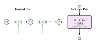
A Deep Equilibrium Model (DEQ) [7] defines its output as the fixed point of a single parametric layer. Given input $𝒙$ , the model computes (DEQ FP) $\begin{matrix} 𝒛^{⋆} = f_{𝜽} (𝒛^{⋆}, 𝒙), \end{matrix}$ where $f_{𝜽} : ℝ^{d} \times ℝ^{n} \to ℝ^{d}$ is a neural network layer (e.g. a Transformer block). The forward pass finds $𝒛^{⋆}$ by applying a root-finding algorithm, such as Broyden's method or Anderson acceleration, to the residual $g (𝒛) = f_{𝜽} (𝒛, 𝒙) - 𝒛 = 0 .$

Conceptually, a DEQ is an infinitely deep, weight-tied network: the same layer $f_{𝜽}$ is applied over and over until the representation converges. The remarkable insight is that we can differentiate through this infinite process using only the fixed point itself.

Theorem 5 (Implicit Differentiation for DEQ).

Let $𝒛^{⋆}$ satisfy and let $J = \frac{\partial f_{𝜽}}{\partial 𝒛} |_{𝒛 = 𝒛^{⋆}} \in ℝ^{d \times d}$ be the Jacobian at the fixed point. For any scalar loss $ℒ (𝒛^{⋆})$ , the gradient with respect to the parameters $𝜽$ is (DEQ GRAD) $\begin{matrix} \frac{\partial ℒ}{\partial 𝜽} = 𝝀^{⊤} \frac{\partial f_{𝜽}}{\partial 𝜽} |_{𝒛 = 𝒛^{⋆}}, \end{matrix}$ where $𝝀 \in ℝ^{d}$ solves the linear system (DEQ Adjoint) $\begin{matrix} (I - J^{⊤}) 𝝀 = (\frac{\partial ℒ}{\partial 𝒛^{⋆}})^{⊤} . \end{matrix}$

Proof.

Define the residual map $F (𝒛, 𝜽) = 𝒛 - f_{𝜽} (𝒛, 𝒙)$ . At the equilibrium $𝒛^{⋆}$ we have $F (𝒛^{⋆}, 𝜽) = 0$ .

Step 1 (Implicit Function Theorem). The Jacobian of $F$ with respect to $𝒛$ is $\frac{\partial F}{\partial 𝒛} |_{𝒛^{⋆}} = I - J .$ If $I - J$ is invertible (which is guaranteed when the spectral radius $ρ (J) < 1$ , i.e. when $f_{𝜽}$ is contractive), then the Implicit Function Theorem asserts that $𝒛^{⋆}$ is a smooth function of $𝜽$ in a neighbourhood, with total derivative (Dzstar Dtheta) $\begin{matrix} \frac{d 𝒛^{⋆}}{d 𝜽} = - (\frac{\partial F}{\partial 𝒛})^{- 1} \frac{\partial F}{\partial 𝜽} = (I - J)^{- 1} \frac{\partial f_{𝜽}}{\partial 𝜽} |_{𝒛^{⋆}} . \end{matrix}$

Step 2 (Chain rule). Applying the chain rule to $ℒ$ : $\frac{\partial ℒ}{\partial 𝜽} = \frac{\partial ℒ}{\partial 𝒛^{⋆}} \frac{d 𝒛^{⋆}}{d 𝜽} = \frac{\partial ℒ}{\partial 𝒛^{⋆}} {(I - J)}^{- 1} \frac{\partial f_{𝜽}}{\partial 𝜽} |_{𝒛^{⋆}} .$

Step 3 (Adjoint formulation). Define the row vector $𝝀^{⊤} = \frac{\partial ℒ}{\partial 𝒛^{⋆}} {(I - J)}^{- 1}$ . Transposing both sides gives $(I - J^{⊤}) 𝝀 = (\frac{\partial ℒ}{\partial 𝒛^{⋆}})^{⊤}$ , which is the linear system . Substituting back: $\frac{\partial ℒ}{\partial 𝜽} = 𝝀^{⊤} \frac{\partial f_{𝜽}}{\partial 𝜽} |_{𝒛^{⋆}} .$ Crucially, the linear system can be solved iteratively: $𝝀_{k + 1} = J^{⊤} 𝝀_{k} + (\partial ℒ / \partial 𝒛^{⋆})^{⊤}$ , which converges when $ρ (J) < 1$ (the same condition that guarantees the forward pass converges). This avoids ever forming or inverting $(I - J)$ explicitly.

∎

Key Idea.

The DEQ insight is profound: an infinitely deep network (weight-tied) converges to a fixed point, and we can backpropagate through this infinite depth using only the fixed point itself, with no need to store intermediate activations. This makes the memory cost independent of “depth.”

Caution.

The DEQ forward pass requires convergence of the root-finding algorithm, which is only guaranteed when $f_{𝜽}$ is contractive (spectral radius $ρ (J) < 1$ ). In practice, spectral normalisation or other regularisation techniques are employed to enforce contractivity during training.

Example 4 (DEQ on a 2D Problem).

Consider a two-dimensional DEQ with $f_{𝜽} (𝒛, 𝒙) = \tanh ([\begin{matrix} 0.3 & 0.1 \\ - 0.2 & 0.4 \end{matrix}] 𝒛 + [\begin{matrix} 1 \\ 1 \end{matrix}] x),$ where $x \in ℝ$ is a scalar input. The weight matrix $W = [\begin{matrix} 0.3 & 0.1 \\ - 0.2 & 0.4 \end{matrix}]$ has spectral norm ${‖ W ‖}_{2} = 0.4515 < 1$ (its singular values are $0.45150$ and $0.31008$ ; the spectral radius is $\sqrt{\det W} = \sqrt{0.14} = 0.3742$ , the eigenvalues being complex), so the composition $\tanh \circ (affine)$ is contractive and the iteration $𝒛_{k + 1} = f_{𝜽} (𝒛_{k}, x)$ converges for any starting point.

For $x = 1$ and $𝒛_{0} = 0$ , the first few iterates are: $\begin{matrix} 𝒛_{1} & = \tanh ([1, 1]^{⊤}) \approx [0.761594, 0.761594]^{⊤}, \\ 𝒛_{2} & \approx [0.862912, 0.818521]^{⊤}, \\ 𝒛_{3} & \approx [0.871846, 0.819346]^{⊤}, \\ 𝒛_{4} & \approx [0.872508, 0.818867]^{⊤} \approx 𝒛^{⋆} = [0.872543, 0.818742]^{⊤} . \end{matrix}$ Convergence is rapid: the successive step sizes $‖ 𝒛_{k} - 𝒛_{k - 1} ‖$ are $1.08$ , $1.16 \times 10^{- 1}$ , $8.97 \times 10^{- 3}$ and $8.17 \times 10^{- 4}$ , so by iteration 4 the step is already below $10^{- 3}$ . The observed ratio between consecutive steps is about $0.08$ to $0.15$ , far better than the global guarantee ${‖ W ‖}_{2} = 0.4515$ , because the rate that governs convergence near the fixed point is the local Jacobian $J = diag (1 - (𝒛^{⋆})^{⊙ 2}) W$ , whose spectral norm here is $0.1479$ : the $\tanh$ is well into its flat region at $𝒛^{⋆}$ , and its derivative shrinks every direction further. (Note that $‖ 𝒛_{k} - 𝒛_{k - 1} ‖$ is the step size; Definition 14 calls $f_{𝜽} (𝒛, x) - 𝒛$ the residual, and the two coincide only up to a shift of the index.)

Left: DEQ forward pass: the same layer

f_{𝜽}

is iterated until the representation converges to

𝒛^{⋆}

. Right: DEQ backward pass: a single linear solve replaces backpropagation-through-time, yielding

O (1)

memory cost regardless of the number of forward iterations.

Recursive Reasoning Architectures

We have seen that Chain-of-Thought adds computational depth by generating tokens sequentially (Theorem 4), and that Deep Equilibrium Models add depth by iterating a single layer to a fixed point (Definition 14). In this section we survey a family of recent architectures that take the idea of explicit recursion even further, achieving remarkable reasoning performance, sometimes with surprisingly few parameters.

Universal Transformers

Definition 15 (Universal Transformer).

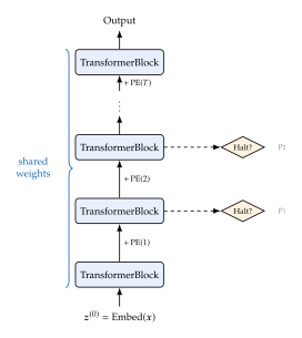
The Universal Transformer [15] applies the same Transformer block repeatedly to the sequence representation: (UT INIT) $\begin{matrix} 𝒛^{(0)} & = Embed (𝒙), \\ 𝒛^{(t)} & = TransformerBlock (𝒛^{(t - 1)} + PE (t)), t = 1, 2, \dots, T, \end{matrix}$ where $PE (t)$ is a per-step coordinate encoding that informs the shared block of the current iteration count, and the block is shared (weight-tied) across all steps $t$ . Note that the encoding enters the block's input: added to the output instead, the block at step $t$ would only ever see $PE (t - 1)$ and could not know which iteration it was on.

Remark 12 (Turing Completeness).

Equipped with Adaptive Computation Time (see below), the Universal Transformer is Turing-complete: it can simulate any Turing machine given sufficient iterations and precision. This stands in stark contrast to the standard (fixed-depth) Transformer, which is limited to the circuit complexity class ${𝖳 𝖢}^{0}$ per Theorem 2. The additional computational power comes entirely from the ability to repeat the same block an unbounded number of times.

The Universal Transformer applies the same block

T

times, with the coordinate encoding

PE (t)

added to the input of application

t

, so that each application knows which step it is on. Optional halting units read

p_{t}

off the output of application

t

and decide when to stop for each position (Adaptive Computation Time).

Adaptive Computation Time

Definition 16 (Adaptive Computation Time).

Adaptive Computation Time (ACT) [16] allows a recurrent model to choose, for each input, how many computation steps to perform. At each step $t$ , the model produces a halting probability $p_{t} \in [0,1]$ via a learned sigmoid unit. The model halts at step $N$ defined by (ACT HALT) $\begin{matrix} N = \min {n | \sum_{t = 1}^{n} p_{t} \geq 1 - ϵ}, \end{matrix}$ for a small threshold $ϵ > 0$ . The remainder $R_{N} = 1 - \sum_{t = 1}^{N - 1} p_{t}$ is assigned to the final step so the weights sum to one. The output is the weighted combination (ACT Output) $\begin{matrix} 𝒚 = \sum_{t = 1}^{N - 1} p_{t} \cdot 𝒉_{t} + R_{N} \cdot 𝒉_{N}, \end{matrix}$ where $𝒉_{t}$ is the hidden state at step $t$ . A ponder cost $𝒫 = N + R_{N}$ is added to the loss to encourage the model to halt early when additional computation is unnecessary.

Remark 13.

ACT provides a differentiable (if approximate) mechanism for the model to learn “how hard to think.” Easy inputs trigger early halting; hard inputs receive more computation steps. This mirrors human cognition, where difficult problems naturally require more deliberation.

Hierarchical Reasoning Model

Definition 17 (Hierarchical Reasoning Model).

The Hierarchical Reasoning Model (HRM) [17] is a single recurrent network of 27 million parameters, trained from scratch on roughly a thousand examples, with no pre-training and no chain-of-thought data. Its two interdependent modules are recurrent modules running at different timescales, not separate models exchanging tokens:

H-module (slow): performs abstract planning, updating once per macro-step on a latent state $𝒛^{H} \in ℝ^{d_{H}}$ .
L-module (fast): performs rapid detailed computation, running $m$ inner updates on $𝒛^{L} \in ℝ^{d_{L}}$ for each H-update, conditioned on the current $𝒛^{H}$ .

Formally, for macro-step $k$ and inner step $j = 1, \dots, m$ : $\begin{matrix} 𝒛_{k, j}^{L} & = L (𝒛_{k, j - 1}^{L}, 𝒛_{k}^{H}, 𝒙), \\ 𝒛_{k + 1}^{H} & = H (𝒛_{k}^{H}, 𝒛_{k, m}^{L}, 𝒙), \end{matrix}$ with $𝒛_{k, 0}^{L} = 𝒛_{k - 1, m}^{L}$ . The entire nested loop runs inside a single forward pass: there is no token-level interface between the two modules, and nothing is emitted until the loop terminates.

Remark 14 (Two Timescales, One Network).

The pattern is reminiscent of the manager–worker decomposition in hierarchical reinforcement learning, with the slow module setting the direction and the fast module filling in the detail. The resemblance is structural rather than architectural: both modules here are small recurrent blocks inside one 27M-parameter network, and the depth that does the reasoning comes from the nesting of the two loops, not from the size of either module.

Tiny Recursive Models

Perhaps the most surprising recent result in reasoning comes from a model with only 7 million parameters.

Definition 18 (Tiny Recursive Model).

A Tiny Recursive Model (TRM) [18] defines reasoning as a fixed-point iteration with a compact neural network: (TRM Iteration) $\begin{matrix} 𝒛_{k + 1} = net (𝒙, 𝒚, 𝒛_{k}), k = 0, 1, 2, \dots \end{matrix}$ where $𝒙$ is the input encoding, $𝒚$ is the (partial) output encoding, $𝒛 \in ℝ^{d}$ is a recurrent latent state, and $net$ is a small neural network; in the original work, as few as 7 million parameters.

Training uses Truncated Backpropagation Through Loops (TBPTL): during training, the iteration is unrolled for $K$ steps and the gradient is propagated through all $K$ steps. At test time, however, the model is free to iterate for many more than $K$ steps, exploiting the convergent nature of the iteration to “think longer” without retraining.

The headline result is remarkable: a 7M-parameter TRM (the attention variant) reaches 44.6% on ARC-AGI-1 under the two-attempt protocol, against DeepSeek-R1's 15.8% at 671B parameters on the same benchmark.

Key Idea.

TRM demonstrates that recursive computation, not parameter count, is the key ingredient for certain types of reasoning. A 7,M-parameter model with enough iterations can outperform a 671,B-parameter model without recursion on abstract reasoning tasks, across a parameter ratio of about $10^{5}$ . The ratio measures storage, not total work: TRM spends many iterations on each answer, so it buys with sequential depth what the larger model would have to buy with width.

Proposition 7 (TRM Convergence).

If $net (𝒙, 𝒚, \cdot)$ is Lipschitz continuous in its third argument with constant $L < 1$ for all fixed $𝒙, 𝒚$ , that is, $‖ net (𝒙, 𝒚, 𝒛) - net (𝒙, 𝒚, 𝒛^{'}) ‖ \leq L ‖ 𝒛 - 𝒛^{'} ‖ \forall 𝒛, 𝒛^{'} \in ℝ^{d},$ then by Theorem 1 the iteration converges to a unique fixed point $𝒛^{⋆} (𝒙, 𝒚)$ for any initialisation $𝒛_{0}$ .

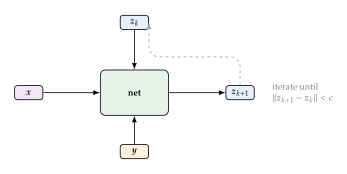
The TRM core loop. A small network net takes the input

𝒙

, partial output

𝒚

, and the current latent state

𝒛_{k}

, producing the next state

𝒛_{k + 1}

. The loop continues until convergence. During training the loop is unrolled for a fixed number of steps (TBPTL); at test time the model may iterate longer.

Universal Reasoning Model

Definition 19 (Universal Reasoning Model).

The Universal Reasoning Model (URM) [19] is a production-scale recursive reasoning architecture built on three design principles:

ConvSwiGLU block. The recursive module combines a short depthwise 1-D convolution (kernel size $k = 2$ ) with the SwiGLU activation. SwiGLU puts the swish on the gate branch and leaves the value branch linear: (URM GATE) $\begin{matrix} 𝑮 & = W_{g} 𝒉 + 𝐛_{g}, \\ 𝑼 & = W_{l} 𝒉 + 𝐛_{l}, \\ SwiGLU (𝒉) & = swish (𝑮) ⊙ 𝑼 = (𝑮 ⊙ σ (𝑮)) ⊙ 𝑼, \end{matrix}$ where $swish (u) = u σ (u)$ , also written $SiLU$ . The full block is $𝒉^{(t)} = ConvSwiGLU (𝒉^{(t - 1)}, 𝒙)$ .
TBPTL training. Like TRM, URM trains with Truncated Backpropagation Through Loops, unrolling for $K$ steps during training.
Adaptive halting. URM uses ACT-style adaptive computation time (Definition 16): a learned halting head accumulates halting probabilities over an outer loop and stops when they cross the threshold, with the loop capped at 16 steps.

URM achieves strong performance on both mathematical reasoning and common-sense benchmarks, demonstrating that recursive architectures scale beyond toy problems.

Remark 15 (URM vs. TRM).

Both models share the core principle of recursive computation through a weight-shared module. URM differs in its use of convolution-based blocks (which capture local structure efficiently), a more sophisticated gating mechanism (SwiGLU), and a learned ACT halting head over its outer loop. URM scales to larger model sizes and more diverse tasks, while TRM emphasises minimality, showing that even 7M parameters suffice for abstract reasoning when coupled with enough iterations.

Comparison and Analysis

Table 1 summarises the key properties of the architectures discussed in this section.

Model	Params	Recursion Type	ARC-AGI-1	Key Innovation
Direct pred (Transformer)	27.3M	None	21.0%	Attention mechanism
DeepSeek-R1 [6]	671B	CoT (token-level)	15.8%	GRPO training
o3-mini-high	undisclosed	CoT (token-level)	34.5%	Test-time scaling
Gemini 2.5 Pro	undisclosed	CoT (token-level)	37.0%	Test-time scaling
HRM [17]	27M	Hierarchical	40.3%	Two timescales, one pass
TRM-MLP [18]	19M	Fixed-point (latent)	29.6%	Tiny net + iteration
TRM-Att [18]	7M	Fixed-point (latent)	44.6%	Tiny net + iteration

Comparison of reasoning architectures. The ARC-AGI column reports accuracy on ARC-AGI-1 under the two-attempt protocol tabulated by Jolicoeur-Martineau [18], so that every entry is measured the same way. “Direct pred” is the non-recurrent Transformer baseline trained with the HRM recipe [17]. URM's published figure is pass@1 rather than two-attempt and is therefore given in the text rather than in this column.

The most striking entry in Table 1 is TRM's performance: 44.6% on ARC-AGI-1 with only 7M parameters, against DeepSeek-R1's 15.8% with 671B, a parameter ratio of $671 \times 10^{9} / 7 \times 10^{6} \approx 10^{5}$ . Two qualifications keep the comparison honest. First, the gain over HRM (40.3% at 27M) is four points, not a revolution: most of the effect comes from the recurrent-fixed-point family rather than from TRM specifically. Second, on the harder ARC-AGI-2 every model in this family is still near the floor: TRM-Att 7.8%, TRM-MLP 2.4%, HRM 5.0%, DeepSeek-R1 1.3%. URM [19] reports the strongest figures in this line of work, 53.8% pass@1 on ARC-AGI-1 and 16.0% pass@1 on ARC-AGI-2, using a 4-layer model of hidden size 512 with 8 heads; its pass@1 protocol is not directly comparable with the two-attempt column above. With those caveats the pattern is unmistakable, and it is strong evidence for a principle that runs through the entire chapter:

Insight.

The ability to reason is determined not by the size of a model's single forward pass but by the depth of its iterated computation. A small model that “thinks” for many steps can outperform a massive model that “thinks” only once. In the language of computational complexity: increasing sequential depth (from ${𝖳 𝖢}^{0}$ toward $𝖯$ ) matters more than increasing parallel width.

Connections and Synthesis

Having surveyed recurrence (Recurrent Foundations for Iterative Computation), prompting strategies, reinforcement learning for reasoning, self-reflection, and recursive architectures, we now step back and identify the common mathematical thread that unites them all.

The Unifying Framework: Reasoning as Fixed-Point Computation

Definition 20 (Iterative Reasoning Operator).

An iterative reasoning system is a triple $(S, T, s_{0})$ consisting of:

A state space $S$ (which may be discrete, continuous, or a hybrid of both).
An operator $T : S \to S$ .
An initial state $s_{0} \in S$ encoding the input.

The system iterates $s_{k + 1} = T (s_{k})$ and extracts the output from the convergence point $s^{⋆}$ (or from $s_{K}$ after a fixed budget $K$ ).

Table 2 shows how every method in this chapter instantiates this framework.

Method	State Space $S$	Operator $T$
RNN (Definition 10)	Hidden state $𝒉 \in ℝ^{d}$	$𝒉_{t} = σ (W_{h} 𝒉_{t - 1} + W_{x} 𝒙_{t} + 𝐛)$
Chain-of-Thought (Definition 6)	Token sequence	LM next-token prediction
Self-Refine (Definition 13)	Output text	Critique $+$ Refine
DEQ (Definition 14)	Latent $𝒛 \in ℝ^{d}$	$𝒛 = f_{𝜽} (𝒛, 𝒙)$
TRM (Definition 18)	Latent $𝒛 \in ℝ^{d}$	$𝒛 = net (𝒙, 𝒚, 𝒛)$
Diffusion LM (sec:diffusion_language)	Masked tokens	Unmask $+$ remask

Every reasoning method as an instance of the iterative reasoning operator framework (Definition 20).

Connection to Diffusion Language Models

Recall from sec:diffusion_language that diffusion language models, such as MDLM and LLaDA, iteratively denoise a sequence: $𝒙^{(T)} \to 𝒙^{(T - 1)} \to \dots \to 𝒙^{(0)} .$ This is structurally identical to the recursive reasoning systems of this chapter:

The state is the partially denoised (partially unmasked) sequence.
The operator is the denoising step: predict masked positions conditioned on the current unmasked context.
The fixed point is the fully clean sequence $𝒙^{(0)}$ .

Insight.

Masked diffusion language models perform a form of implicit reasoning: each denoising step considers the full context of unmasked tokens to predict masked positions, effectively “deliberating” over multiple passes. This is precisely the multi-pass computation that elevates the model beyond ${𝖳 𝖢}^{0}$ (Theorem 2). From the perspective of this chapter, a diffusion language model is a reasoning system whose “chain of thought” lives in token-masking space rather than in token-generation space.

The Parallelism–Depth Trade-off

Proposition 8 (Parallelism–Depth Trade-off).

For any computational task, there is a fundamental trade-off between sequential depth and parallel work [8]:

A single forward pass through a Transformer computes in $O (1)$ sequential depth¹ but $O (n^{2})$ parallel work (self-attention over $n$ tokens).
Chain-of-Thought with $T$ reasoning tokens adds $O (T)$ sequential depth with $O (T \cdot n^{2})$ total work.
Recursive models (TRM/URM) with $K$ iterations add $O (K)$ sequential depth. One iteration of a $d$ -dimensional block costs $Θ (d^{2})$ per token for its dense maps plus $Θ (n d)$ for attention over $n$ tokens, so the total is $O (K (d^{2} + n d))$ per token, where $d$ is the latent dimension.

More sequential depth enables the solution of harder problems (moving from ${𝖳 𝖢}^{0}$ toward $𝖯$ ), but reduces the opportunities for parallelism and increases latency.

This trade-off is central to the practical deployment of reasoning systems: how much time should a model spend “thinking”? ACT (Definition 16), used both by the Universal Transformer and by URM (Definition 19), is the standard mechanism for navigating this trade-off adaptively.

Open Problems

The study of reasoning in neural networks is young and rich with open questions. We highlight several that we believe are particularly important.

Problem 1 (Open Problems in Neural Reasoning).

Optimal depth allocation. How should a model decide how many reasoning steps to use for a given input? Learned halting heads such as ACT are heuristics; is there a principled, information-theoretic criterion?
Verifiable reasoning. Can we verify that a chain of thought is logically sound, rather than merely checking that it produces the correct final answer? Current models can arrive at the right answer for wrong reasons.
Compositionality. Can recursive models compose learned subroutines into novel reasoning chains? For example, can a model that has learned “sort” and “search” compose them into “sort then search”?
Theoretical limits of bounded recursion. What is the computational complexity class of a TRM whose operator has fixed size, independent of the input length, run for $K$ iterations with $K$ polynomial in the input size? Is it exactly $𝖯$ , or some proper subclass? (The size restriction matters: allow the operator to grow with $n$ and the answer is immediate, since one iteration can then implement a Turing-machine transition step.)
Reasoning in continuous spaces. Can latent-space reasoning (as in TRM and DEQ) be connected to continuous optimisation? Is finding a fixed point equivalent to minimising some implicit loss?
Self-improvement. Can a recursive reasoning model improve its own operator $T$ during inference, rather than relying on a fixed, trained operator?
Connection to consciousness. Is iterative self-monitoring (Reflexion, self-consistency checking) related to computational models of consciousness such as Global Workspace Theory?
Scaling laws for depth vs. width. What are the scaling laws when we increase reasoning depth (number of iterations or CoT tokens) vs. model size (number of parameters)? Existing scaling laws [20] focus on parameters, data and training compute; extending them to “thinking time” is an open frontier.

We close this section with a conjecture that, if true, would place recursive reasoning on firm computational-theoretic foundations.

Conjecture 1 (Latent Reasoning Hypothesis).

There is a fixed operator $net : ℝ^{n} \times ℝ^{d} \to ℝ^{d}$ , of size independent of the input length $n$ , and a polynomial $K (n)$ , such that for every decision problem in $𝖯$ the recursive iteration $𝒛_{k + 1} = net (𝒙, 𝒛_{k}), 𝒛_{0} = 0,$ run for $K (n)$ steps, solves the problem for all inputs $𝒙$ of length $n$ , and such an operator is learnable from a polynomial number of examples.

Remark 16.

The size restriction is what makes the statement a conjecture. Drop it, and the result follows immediately from the construction already given for Theorem 4: let $𝒛_{k}$ encode the configuration of a polynomial-time Turing machine, let $net$ be the polynomial-size circuit implementing one transition step, and run $K = p (n)$ iterations. The same construction answers open problem 4 above under the same non-uniform reading, which is why that problem too should be read with a fixed-size operator. The interesting content is that models such as TRM hold their operator fixed at 7,M parameters across every problem instance and learn it, which is a far stronger claim than mere existence.

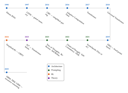
Historical Timeline

The ideas in this chapter span over three decades, from the earliest recurrent networks to the latest recursive reasoning architectures. fig:reasoning-timeline presents a chronological overview, colour-coded by category: defblueblue for architectures, thmgreengreen for prompting and inference methods, exorangeorange for reinforcement learning approaches, and lempurplepurple for theoretical results.

Historical timeline of ideas in recurrence, recursion, and reasoning. The field has shifted from building recurrence into the architecture (1990s–2010s), to eliciting reasoning through prompting (2021–2023), to training for reasoning via RL (2023–2025), and most recently to purpose-built recursive reasoning architectures (2025). Colour key: blue = architecture, green = prompting/inference, orange = reinforcement learning, purple = theory.

Exercises

Exercise 4 (Fixed-Point Iteration).

Consider the map $T (x) = \cos (x)$ on the interval $[0, 1]$ .

Show that $T$ is a contraction on $[0, 1]$ . Hint: use the Mean Value Theorem and the bound $| \sin (x) | \leq \sin (1) < 1$ for $x \in [0,1]$ .
Starting from $x_{0} = 0$ , compute $x_{1}, x_{2}, \dots, x_{5}$ .
Estimate the fixed point $x^{⋆}$ (the Dottie number) and verify that $\cos (x^{⋆}) = x^{⋆}$ to three decimal places.

Exercise 5 (GRU vs. LSTM).

Couple the LSTM's gates (Definition 11) by setting $𝒇_{t} = 1 - 𝒛_{t}$ and $𝒊_{t} = 𝒛_{t}$ , and hold the output gate open, $𝒐_{t} = 1$ . The result is the coupled input-forget gate (CIFG) LSTM.

Write out the LSTM equations under these constraints and simplify.
Show that CIFG is close to, but not identical with, the GRU (Definition 1), and identify exactly two remaining differences. Hint: the book's LSTM has $𝒉_{t} = 𝒐_{t} ⊙ \tanh (𝒄_{t})$ , so $𝒐_{t} = 1$ leaves $𝒉_{t} = \tanh (𝒄_{t})$ rather than $𝒉_{t} = 𝒄_{t}$ ; and the GRU's reset gate $𝒓_{t}$ , which gates $𝒉_{t - 1}$ inside the candidate, has no LSTM counterpart.
What is the advantage of coupling the gates in this way? Discuss in terms of parameter count and gradient flow.

Exercise 6 (Vanishing Gradients in Vanilla RNNs).

For the vanilla RNN $𝒉_{t} = \tanh (W_{h} 𝒉_{t - 1} + W_{x} 𝒙_{t})$ :

Show that the Jacobian satisfies $\frac{\partial 𝒉_{t}}{\partial 𝒉_{t - 1}} = diag (1 - 𝒉_{t}^{2}) W_{h}$ .
Conclude that $‖ \frac{\partial 𝒉_{T}}{\partial 𝒉_{t}} ‖ \leq σ_{\max} (W_{h})^{T - t}$ where $σ_{\max} (W_{h})$ is the spectral norm of $W_{h}$ .
Discuss the implications for learning long-range dependencies when $σ_{\max} (W_{h}) < 1$ versus $σ_{\max} (W_{h}) > 1$ .

Exercise 7 ( ${𝖳 𝖢}^{0}$ and Parity).

Prove that the parity function on $n$ bits cannot be computed by an ${𝖠 𝖢}^{0}$ circuit. You may use H stad's Switching Lemma without proof.
Explain why this does not exclude parity from ${𝖳 𝖢}^{0}$ . Hint: What additional gate type does ${𝖳 𝖢}^{0}$ allow?
Construct an explicit ${𝖳 𝖢}^{0}$ circuit (constant depth, polynomial size, with threshold gates) that computes parity.

Exercise 8 (CoT Depth).

A computational problem requires $Θ (n)$ sequential computation steps (it is in $𝖯$ but not in ${𝖭 𝖢}^{1}$ ).

Using Theorem 4, how many CoT tokens must a Transformer generate to solve this problem?
If the cost of generating each token is $O (n^{2})$ (due to attention), what is the total cost? Compare to the cost of a direct $O (n)$ algorithm.
Discuss the implications for the efficiency of CoT-based reasoning.

Exercise 9 (Self-Consistency Error Bound).

Generalise the self-consistency result to the case where there are $C > 2$ possible answers. Let the correct answer have probability $p$ and let the strongest competitor have probability $q_{\max} = \max_{j \neq ⋆} q_{j}$ , with margin $γ = p - q_{\max} > 0$ .

If we draw $K$ independent samples and take a plurality vote, express the error probability as a sum involving the multinomial distribution.
Show that a margin over $1 / C$ is not enough to control the error. Take $C = 3$ with $p = 0.40$ , $q = 0.39$ , $r = 0.21$ and $K = 1000$ , and compute $\Pr [N_{2} > N_{1}]$ exactly by conditioning on $m = N_{1} + N_{2}$ and using $N_{1} | m \sim Bin (m, p / (p + q))$ . You should find an error probability of about $0.354$ , which does not shrink with $K$ in the way a bound in $p - 1 / C$ would predict. Explain why: a plurality vote fails when some other answer outpolls the correct one, so the controlling quantity is the margin over the runner-up, not over $1 / C$ .
Apply Hoeffding to each pairwise difference and a union bound over the $C - 1$ wrong answers to prove $\Pr [error] \leq (C - 1) \exp (- K γ^{2} / 2)$ .
How many samples $K$ does that bound require for error probability $δ$ ?

Exercise 10 (GRPO vs. PPO).

Consider a simple one-step bandit problem with reward $r$ drawn from a distribution with mean $μ$ and variance $σ^{2}$ .

Write the GRPO advantage estimator (Definition 11) for a group of $G$ samples: ${\hat{A}}_{i} = (r_{i} - \overline{r}) / s$ where $\overline{r}$ and $s$ are the sample mean and standard deviation.
Write the PPO advantage for the same setting: ${\hat{A}}_{i} = r_{i} - V (s)$ where $V (s)$ is a learned value baseline.
Compute $Var [{\hat{A}}_{i}]$ for both estimators. Under what conditions does GRPO have lower variance?
Discuss the trade-off: GRPO avoids learning a value function but requires multiple samples per prompt.

Exercise 11 (DEQ Forward Pass).

Consider a DEQ with $f_{𝜽} (𝒛, 𝒙) = \tanh (W 𝒛 + U 𝒙 + 𝐛)$ where $W \in ℝ^{d \times d}$ , $U \in ℝ^{d \times n}$ , $𝐛 \in ℝ^{d}$ .

Implement (in pseudocode) the forward pass: iterate $𝒛_{k + 1} = f_{𝜽} (𝒛_{k}, 𝒙)$ from $𝒛_{0} = 0$ until $‖ 𝒛_{k + 1} - 𝒛_{k} ‖ < ϵ$ .
Under what condition on $W$ does the iteration converge for any $𝒙$ ? Hint: consider ${‖ W ‖}_{2}$ and the Lipschitz constant of $\tanh$ .
If ${‖ W ‖}_{2} = 0.8$ , estimate the number of iterations needed to reach $ϵ = 10^{- 6}$ accuracy.

Exercise 12 (DEQ Backward Pass).

Continuing from the previous exercise:

Compute the Jacobian $J = \frac{\partial f_{𝜽}}{\partial 𝒛} |_{𝒛^{⋆}}$ for the given $f_{𝜽}$ .
Write the linear system $(I - J^{⊤}) 𝝀 = {(\partial ℒ / \partial 𝒛^{⋆})}^{⊤}$ from Theorem 5.
Show that this system can be solved by the fixed-point iteration $𝝀_{k + 1} = J^{⊤} 𝝀_{k} + {(\partial ℒ / \partial 𝒛^{⋆})}^{⊤}$ . Under what condition does this iteration converge?
Compare the memory cost of this approach to standard backpropagation through $K$ unrolled iterations.

Exercise 13 (TRM Convergence).

A TRM uses the network $net (𝒙, 𝒚, 𝒛) = ReLU (A 𝒛 + B 𝒙 + C 𝒚 + 𝐝)$ where $A \in ℝ^{d \times d}$ .

Show that $ReLU$ is Lipschitz with constant 1.
Conclude that $net (𝒙, 𝒚, \cdot)$ is Lipschitz in $𝒛$ with constant ${‖ A ‖}_{2}$ .
If ${‖ A ‖}_{2} < 1$ , apply Theorem 1 to prove convergence of the TRM iteration to a unique fixed point.
What happens if ${‖ A ‖}_{2} = 1$ ? Give a concrete 1D example where the iteration does not converge.

Exercise 14 (Recursion vs. Parameters).

A standard Transformer with $N$ parameters performs a single forward pass at cost $O (N)$ . A TRM with $n ≪ N$ parameters iterates $K$ times, each iteration costing $O (n)$ .

What is the total compute of the TRM?
For what ratio $K n / N$ does the TRM have lower total compute than the Transformer?
DeepSeek-R1 has $N = 671 \times 10^{9}$ parameters. TRM has $n = 7 \times 10^{6}$ . If TRM uses $K = 1000$ iterations, compute the ratio $K n / N$ . Discuss the implications for “thinking time” vs. “model size.”
Is compute the right metric? Discuss latency implications.

Exercise 15 (Diffusion as Recursion).

Consider a masked diffusion language model that iterates for $T$ denoising steps, unmasking tokens at each step.

Define the state space $S$ and operator $T$ for this model in the framework of Definition 20.
Under what conditions can the denoising operator be viewed as a contraction mapping? Hint: think about the number of masked tokens decreasing monotonically.
Relate the number of diffusion steps to the “reasoning depth” concept developed in this chapter. How does this compare to the number of CoT tokens?

Exercise 16 (Self-Refine Convergence).

Model Self-Refine as the iteration $y_{k + 1} = T (y_{k})$ where $T$ represents the critique-then-refine step.

In what metric space might $T$ be contractive? Propose a concrete metric on the space of text outputs (e.g. edit distance, BLEU-based distance, or embedding distance).
If $T$ is contractive with constant $L = 0.9$ , how many iterations are needed to reduce the “error” $d (y_{k}, y^{⋆})$ below $ϵ = 0.01$ , starting from $d (y_{0}, y^{⋆}) = 1$ ?
What happens if $L > 1$ ? Give an informal example of a critique-refine loop that diverges.
Is the contractivity assumption realistic for language models? Discuss.

Exercise 17 (Tree of Thoughts Complexity).

In Tree of Thoughts (ToT) with branching factor $b$ and maximum depth $d$ :

If each node evaluation costs $c$ (one LM call), what is the total cost of a full BFS?
If we keep only the top- $k$ nodes at each depth (beam search), how does the cost change? Express in terms of $b$ , $d$ , $k$ , and $c$ .
Compare the cost of beam-search ToT ( $k$ beams, depth $d$ ) with Self-Consistency using $K$ samples of a CoT of length $d$ .
Under what conditions does ToT outperform Self-Consistency despite higher cost?

Exercise 18 (Open Problem: Universal Recursive Reasoning).

This is a research-level exercise. Conjecture 1 states that small recursive networks can solve any problem in $𝖯$ .

Prove the conjecture for the special case of problems in ${𝖭 𝖢}^{1}$ . Hint: ${𝖭 𝖢}^{1}$ problems have $O (\log n)$ -depth circuits of polynomial size. Show that a recursive network can simulate one circuit layer per iteration, using $O (\log n)$ iterations total.
Explain why the general case (arbitrary $𝖯$ ) is significantly harder. What is the gap between ${𝖭 𝖢}^{1}$ and $𝖯$ , and what does it imply for the number of iterations?
Discuss whether the conjecture might be false. What would a counterexample look like?

Notes

Here “depth” means the number of serial computation steps, not the number of layers; from a circuit perspective the layers execute in constant serial depth.

References

Computing Machinery and Intelligence

Alan M. Turing

Mind, vol. 59, no. 236, pp. 433-460 · 1950

BibTeX

@article{turing1950computing,
  title={Computing Machinery and Intelligence},
  author={Turing, Alan M.},
  journal={Mind},
  volume={59},
  number={236},
  pages={433--460},
  year={1950}
}

Journal article

Finding Structure in Time

Jeffrey L. Elman

Cognitive Science, vol. 14, no. 2, pp. 179-211 · 1990

BibTeX

@article{elman1990finding,
  title={Finding Structure in Time},
  author={Elman, Jeffrey L.},
  journal={Cognitive Science},
  volume={14},
  number={2},
  pages={179--211},
  year={1990},
  publisher={Wiley Online Library}
}

Journal article

Long Short-Term Memory

Sepp Hochreiter, Jurgen Schmidhuber

Neural Computation, vol. 9, no. 8, pp. 1735-1780 · 1997

BibTeX

@article{hochreiter1997long,
  title={Long Short-Term Memory},
  author={Hochreiter, Sepp and Schmidhuber, J{\"u}rgen},
  journal={Neural Computation},
  volume={9},
  number={8},
  pages={1735--1780},
  year={1997}
}

Journal article

Attention is all you need

Ashish Vaswani, Noam Shazeer, Niki Parmar, Jakob Uszkoreit, Llion Jones, Aidan N Gomez, Lukasz Kaiser, Illia Polosukhin

Advances in neural information processing systems, pp. 5998-6008 · 2017

BibTeX

@inproceedings{vaswani2017attention,
title={Attention is all you need},
author={Vaswani, Ashish and Shazeer, Noam and Parmar, Niki and Uszkoreit, Jakob and Jones, Llion and Gomez, Aidan N and Kaiser, {\L}ukasz and Polosukhin, Illia},
booktitle={Advances in neural information processing systems},
pages={5998--6008},
year={2017}
}

Conference paper

Chain-of-Thought Prompting Elicits Reasoning in Large Language Models

Jason Wei, Xuezhi Wang, Dale Schuurmans, Maarten Bosma, Brian Ichter, Fei Xia, Ed Chi, Quoc Le, et al.

Advances in Neural Information Processing Systems, vol. 35, pp. 24824-24837 · 2022

BibTeX

@article{wei2022chain,
  title={Chain-of-Thought Prompting Elicits Reasoning in Large Language Models},
  author={Wei, Jason and Wang, Xuezhi and Schuurmans, Dale and Bosma, Maarten and Ichter, Brian and Xia, Fei and Chi, Ed and Le, Quoc and Zhou, Denny},
  journal={Advances in Neural Information Processing Systems},
  volume={35},
  pages={24824--24837},
  year={2022}
}

Journal article

DeepSeek-R1: Incentivizing Reasoning Capability in LLMs via Reinforcement Learning

DeepSeek-AI

arXiv preprint arXiv:2501.12948 · 2025

BibTeX

@article{deepseekr1,
  title={{DeepSeek-R1}: Incentivizing Reasoning Capability in {LLMs} via Reinforcement Learning},
  author={{DeepSeek-AI}},
  journal={arXiv preprint arXiv:2501.12948},
  year={2025}
}

Journal article

Deep Equilibrium Models

Shaojie Bai, J. Zico Kolter, Vladlen Koltun

Advances in Neural Information Processing Systems, vol. 32 · 2019

BibTeX

@article{bai2019deep,
  title={Deep Equilibrium Models},
  author={Bai, Shaojie and Kolter, J. Zico and Koltun, Vladlen},
  journal={Advances in Neural Information Processing Systems},
  volume={32},
  year={2019}
}

Journal article

The Parallelism Tradeoff: Limitations of Log-Precision Transformers

William Merrill, Ashish Sabharwal

Transactions of the Association for Computational Linguistics, vol. 11, pp. 531-545 · 2023

BibTeX

@article{merrill2023parallelism,
  title={The Parallelism Tradeoff: Limitations of Log-Precision Transformers},
  author={Merrill, William and Sabharwal, Ashish},
  journal={Transactions of the Association for Computational Linguistics},
  volume={11},
  pages={531--545},
  year={2023}
}

Journal article

Towards Revealing the Mystery behind Chain of Thought: A Theoretical Perspective

Guhao Feng, Bohang Zhang, Yuntian Gu, Haotian Ye, Di He, Liwei Wang

Advances in Neural Information Processing Systems, vol. 36 · 2023

BibTeX

@article{feng2023towards,
  title={Towards Revealing the Mystery behind Chain of Thought: A Theoretical Perspective},
  author={Feng, Guhao and Zhang, Bohang and Gu, Yuntian and Ye, Haotian and He, Di and Wang, Liwei},
  journal={Advances in Neural Information Processing Systems},
  volume={36},
  year={2023}
}

Journal article

Chain of Thought Empowers Transformers to Solve Inherently Serial Problems

Zhiyuan Li, Hong Liu, Denny Zhou, Tengyu Ma

arXiv preprint arXiv:2402.12875 · 2024

BibTeX

@article{li2024chain,
  title={Chain of Thought Empowers Transformers to Solve Inherently Serial Problems},
  author={Li, Zhiyuan and Liu, Hong and Zhou, Denny and Ma, Tengyu},
  journal={arXiv preprint arXiv:2402.12875},
  year={2024}
}

Journal article

Tree of Thoughts: Deliberate Problem Solving with Large Language Models

Shunyu Yao, Dian Yu, Jeffrey Zhao, Izhak Shafran, Thomas L. Griffiths, Yuan Cao, Karthik Narasimhan

Advances in Neural Information Processing Systems, vol. 36 · 2023

BibTeX

@article{yao2023tree,
  title={Tree of Thoughts: Deliberate Problem Solving with Large Language Models},
  author={Yao, Shunyu and Yu, Dian and Zhao, Jeffrey and Shafran, Izhak and Griffiths, Thomas L. and Cao, Yuan and Narasimhan, Karthik},
  journal={Advances in Neural Information Processing Systems},
  volume={36},
  year={2023}
}

Journal article

Simple Statistical Gradient-Following Algorithms for Connectionist Reinforcement Learning

Ronald J. Williams

Machine Learning, vol. 8, no. 3--4, pp. 229-256 · 1992

BibTeX

@article{williams1992simple,
  title={Simple Statistical Gradient-Following Algorithms for Connectionist Reinforcement Learning},
  author={Williams, Ronald J.},
  journal={Machine Learning},
  volume={8},
  number={3--4},
  pages={229--256},
  year={1992}
}

Journal article

Proximal Policy Optimization Algorithms

John Schulman, Filip Wolski, Prafulla Dhariwal, Alec Radford, Oleg Klimov

arXiv preprint arXiv:1707.06347 · 2017

BibTeX

@inproceedings{schulman2017proximal,
  title={Proximal Policy Optimization Algorithms},
  author={Schulman, John and Wolski, Filip and Dhariwal, Prafulla and Radford, Alec and Klimov, Oleg},
  booktitle={arXiv preprint arXiv:1707.06347},
  year={2017}
}

Conference paper

Reflexion: Language Agents with Verbal Reinforcement Learning

Noah Shinn, Federico Cassano, Ashwin Gopinath, Karthik Narasimhan, Shunyu Yao

Advances in Neural Information Processing Systems, vol. 36 · 2023

BibTeX

@article{shinn2023reflexion,
  title={Reflexion: Language Agents with Verbal Reinforcement Learning},
  author={Shinn, Noah and Cassano, Federico and Gopinath, Ashwin and Narasimhan, Karthik and Yao, Shunyu},
  journal={Advances in Neural Information Processing Systems},
  volume={36},
  year={2023}
}

Journal article

Universal Transformers

Mostafa Dehghani, Stephan Gouws, Oriol Vinyals, Jakob Uszkoreit, Lukasz Kaiser

International Conference on Learning Representations · 2019

BibTeX

@inproceedings{dehghani2018universal,
  title={Universal Transformers},
  author={Dehghani, Mostafa and Gouws, Stephan and Vinyals, Oriol and Uszkoreit, Jakob and Kaiser, {\L}ukasz},
  booktitle={International Conference on Learning Representations},
  year={2019}
}

Conference paper

Adaptive Computation Time for Recurrent Neural Networks

Alex Graves

arXiv preprint arXiv:1603.08983 · 2016

BibTeX

@article{graves2016adaptive,
  title={Adaptive Computation Time for Recurrent Neural Networks},
  author={Graves, Alex},
  journal={arXiv preprint arXiv:1603.08983},
  year={2016}
}

Journal article

Hierarchical Reasoning Model

Guan Wang, Jin Li, Yuhao Sun, Xing Chen, Changling Liu, Yue Wu, Meng Lu, Sen Song, et al.

arXiv preprint arXiv:2506.21734 · 2025

BibTeX

@article{wang2025hrm,
  title={Hierarchical Reasoning Model},
  author={Wang, Guan and Li, Jin and Sun, Yuhao and Chen, Xing and Liu, Changling and Wu, Yue and Lu, Meng and Song, Sen and Abbasi Yadkori, Yasin},
  journal={arXiv preprint arXiv:2506.21734},
  year={2025}
}

Journal article

Less is More: Recursive Reasoning with Tiny Networks

Alexia Jolicoeur-Martineau

arXiv preprint arXiv:2510.04871 · 2025

BibTeX

@article{jolicoeur2025trm,
  title={Less is More: Recursive Reasoning with Tiny Networks},
  author={Jolicoeur-Martineau, Alexia},
  journal={arXiv preprint arXiv:2510.04871},
  year={2025}
}

Journal article

Universal Reasoning Model

Zitian Gao, Lynx Chen, Yihao Xiao, He Xing, Ran Tao, Haoming Luo, Joey Zhou, Bryan Dai

arXiv preprint arXiv:2512.14693 · 2025

BibTeX

@article{gao2025urm,
  title={Universal Reasoning Model},
  author={Gao, Zitian and Chen, Lynx and Xiao, Yihao and Xing, He and Tao, Ran and Luo, Haoming and Zhou, Joey and Dai, Bryan},
  journal={arXiv preprint arXiv:2512.14693},
  year={2025}
}

Journal article

Scaling Laws for Neural Language Models

Jared Kaplan, Sam McCandlish, Tom Henighan, Tom B. Brown, Benjamin Chess, Rewon Child, Scott Gray, Alec Radford, et al.

arXiv preprint arXiv:2001.08361 · 2020

BibTeX

@article{kaplan2020scaling,
  title={Scaling Laws for Neural Language Models},
  author={Kaplan, Jared and McCandlish, Sam and Henighan, Tom and Brown, Tom B. and Chess, Benjamin and Child, Rewon and Gray, Scott and Radford, Alec and Wu, Jeffrey and Amodei, Dario},
  journal={arXiv preprint arXiv:2001.08361},
  year={2020}
}

Journal article

Learning Phrase Representations using RNN Encoder--Decoder for Statistical Machine Translation

Kyunghyun Cho, Bart van Merrienboer, Caglar Gulcehre, Dzmitry Bahdanau, Fethi Bougares, Holger Schwenk, Yoshua Bengio

Proceedings of the 2014 Conference on Empirical Methods in Natural Language Processing (EMNLP), pp. 1724-1734 · 2014

BibTeX

@inproceedings{cho2014learning,
  title={Learning Phrase Representations using {RNN} Encoder--Decoder for Statistical Machine Translation},
  author={Cho, Kyunghyun and van Merrienboer, Bart and Gulcehre, Caglar and Bahdanau, Dzmitry and Bougares, Fethi and Schwenk, Holger and Bengio, Yoshua},
  booktitle={Proceedings of the 2014 Conference on Empirical Methods in Natural Language Processing (EMNLP)},
  pages={1724--1734},
  year={2014}
}

Conference paper

Sur les operations dans les ensembles abstraits et leur application aux equations integrales

Stefan Banach

Fundamenta Mathematicae, vol. 3, no. 1, pp. 133-181 · 1922

BibTeX

@article{banach1922operations,
  title={Sur les op{\'e}rations dans les ensembles abstraits et leur application aux {\'e}quations int{\'e}grales},
  author={Banach, Stefan},
  journal={Fundamenta Mathematicae},
  volume={3},
  number={1},
  pages={133--181},
  year={1922}
}

Journal article

Show Your Work: Scratchpads for Intermediate Computation with Language Models

Maxwell Nye, Anders Johan Andreassen, Guy Gur-Ari, Henryk Michalewski, Jacob Austin, David Biber, David Dohan, Aitor Lewkowycz, et al.

arXiv preprint arXiv:2112.00114 · 2021

BibTeX

@article{nye2021show,
  title={Show Your Work: Scratchpads for Intermediate Computation with Language Models},
  author={Nye, Maxwell and Andreassen, Anders Johan and Gur-Ari, Guy and Michalewski, Henryk and Austin, Jacob and Biber, David and Dohan, David and Lewkowycz, Aitor and Bosma, Maarten and Luan, David and others},
  journal={arXiv preprint arXiv:2112.00114},
  year={2021}
}

Journal article

Large Language Models are Zero-Shot Reasoners

Takeshi Kojima, Shixiang Shane Gu, Machel Reid, Yutaka Matsuo, Yusuke Iwasawa

Advances in Neural Information Processing Systems, vol. 35, pp. 22199-22213 · 2022

BibTeX

@article{kojima2022large,
  title={Large Language Models are Zero-Shot Reasoners},
  author={Kojima, Takeshi and Gu, Shixiang Shane and Reid, Machel and Matsuo, Yutaka and Iwasawa, Yusuke},
  journal={Advances in Neural Information Processing Systems},
  volume={35},
  pages={22199--22213},
  year={2022}
}

Journal article

Self-Consistency Improves Chain of Thought Reasoning in Language Models

Xuezhi Wang, Jason Wei, Dale Schuurmans, Quoc Le, Ed Chi, Sharan Narang, Aakanksha Chowdhery, Denny Zhou

International Conference on Learning Representations · 2023

BibTeX

@article{wang2023selfconsistency,
  title={Self-Consistency Improves Chain of Thought Reasoning in Language Models},
  author={Wang, Xuezhi and Wei, Jason and Schuurmans, Dale and Le, Quoc and Chi, Ed and Narang, Sharan and Chowdhery, Aakanksha and Zhou, Denny},
  journal={International Conference on Learning Representations},
  year={2023}
}

Journal article

STaR: Bootstrapping Reasoning With Reasoning

Eric Zelikman, Yuhuai Wu, Jesse Mu, Noah D. Goodman

Advances in Neural Information Processing Systems, vol. 35, pp. 15476-15488 · 2022

BibTeX

@article{zelikman2022star,
  title={{STaR}: Bootstrapping Reasoning With Reasoning},
  author={Zelikman, Eric and Wu, Yuhuai and Mu, Jesse and Goodman, Noah D.},
  journal={Advances in Neural Information Processing Systems},
  volume={35},
  pages={15476--15488},
  year={2022}
}

Journal article

DeepSeekMath: Pushing the Limits of Mathematical Reasoning in Open Language Models

Zhihong Shao, Peiyi Wang, Qihao Zhu, Runxin Xu, Junxiao Song, Mingchuan Zhang, Y.K. Li, Y. Wu, et al.

arXiv preprint arXiv:2402.03300 · 2024

BibTeX

@article{shao2024deepseekmath,
  title={{DeepSeekMath}: Pushing the Limits of Mathematical Reasoning in Open Language Models},
  author={Shao, Zhihong and Wang, Peiyi and Zhu, Qihao and Xu, Runxin and Song, Junxiao and Zhang, Mingchuan and Li, Y.K. and Wu, Y. and Guo, Daya},
  journal={arXiv preprint arXiv:2402.03300},
  year={2024}
}

Journal article

Self-Refine: Iterative Refinement with Self-Feedback

Aman Madaan, Niket Tandon, Prakhar Gupta, Skyler Hallinan, Luyu Gao, Sarah Wiegreffe, Uri Alon, Nouha Dziri, et al.

Advances in Neural Information Processing Systems, vol. 36 · 2023

BibTeX

@article{madaan2023self,
  title={Self-Refine: Iterative Refinement with Self-Feedback},
  author={Madaan, Aman and Tandon, Niket and Gupta, Prakhar and Hallinan, Skyler and Gao, Luyu and Wiegreffe, Sarah and Alon, Uri and Dziri, Nouha and Prabhumoye, Shrimai and Yang, Yiming and others},
  journal={Advances in Neural Information Processing Systems},
  volume={36},
  year={2023}
}

Journal article

← 22 Diffusion Language Models 24 Memory Management for Large Language Models →