22 Diffusion Language Models
Introduction and Motivation
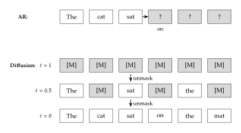
Language generation has been dominated by autoregressive (AR) models. From early recurrent neural networks to modern Transformers such as GPT [12], LLaMA [13], and their successors, the dominant paradigm is simple: generate text one token at a time, left to right, by factoring the joint probability as (AR Factorization) where is a sequence of tokens from a vocabulary of size . This factorization is exact by the chain rule of probability; no approximation is needed. Training is straightforward via teacher forcing, and generation proceeds token by token.
Yet this very simplicity conceals fundamental limitations. Consider the following:
Sequential bottleneck. Generating tokens requires serial forward passes through the network. Each pass is memory-bandwidth bound on modern GPUs, leading to poor hardware utilization. Even with a peak of order FLOP/s available, the GPU sits mostly idle waiting for memory.
Left-to-right commitment. Once a token is generated, it cannot be revised. The model must commit to each word before seeing the rest of the sentence. Humans do not write this way; we draft, revise, and refine.
The reversal curse. Autoregressive models trained on “A is B” struggle to answer “What is B?” with “A”, because the left-to-right factorization never conditions on the latter part of a sequence to predict the former [1].
No native infilling. Filling in a blank in the middle of a sentence requires special training modifications (fill-in-the-middle) that are not part of the natural AR framework.
Meanwhile, in the domain of images, diffusion models have achieved spectacular success. Models like DDPM [14], Stable Diffusion [15], and DALL-E [16] generate images by iteratively denoising from pure noise, producing all pixels simultaneously rather than one at a time. The quality of generated images has surpassed that of GANs in many settings. This raises a natural question:
[colback=defbluebg, colframe=defblue, boxrule=0.8pt] Central Question: Can we build diffusion models for language that rival or surpass autoregressive LLMs, while gaining the benefits of parallel generation, bidirectional context, and iterative refinement?
This chapter tells the story of how this question has been progressively answered. We begin by reviewing the key background: diffusion models for images, and the classical masked autoregressive models that foreshadow many ideas in diffusion language models. We then identify the fundamental challenge (language is discrete, not continuous) and show how this challenge has been addressed through discrete diffusion processes, culminating in the modern masked diffusion language models (MDLMs). We trace the development from D3PM [17] through MDLM [18] and SEDD [19] to the large-scale LLaDA [5], LLaDA 2.0 [20], and Mercury [8] models. Along the way, we present detailed mathematical derivations, TikZ diagrams of the key processes, and discussions of the practical advantages and challenges.
Background: Autoregressive and Masked Models
Before diving into diffusion, it is instructive to review the classical masked and autoregressive generative models for sequences. These models share deep connections with diffusion language models, and understanding them provides essential intuition.
Autoregressive Models: NADE, MADE, PixelRNN, PixelCNN
The autoregressive factorization is the backbone of many generative models. The key design choice is how to parameterize each conditional .
NADE (Neural Autoregressive Density Estimation).
NADE [21] models each conditional using a single-hidden-layer neural network that shares parameters across positions. For a -dimensional binary vector : where is the sigmoid function, and are weight matrices, and and are bias vectors. The crucial feature is that the hidden activation depends only on the preceding variables , enforcing the autoregressive property.
Remark 1.
NADE requires forward passes to compute the full density and to generate all dimensions, since each conditional depends on the previous outputs. This sequential nature is the same bottleneck that plagues all autoregressive models.
MADE (Masked Autoencoder for Distribution Estimation).
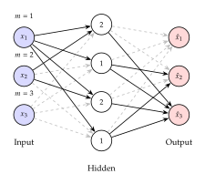
MADE [22] achieves the autoregressive property in a single forward pass by applying carefully designed binary masks to the weight matrices of a standard autoencoder. Each input unit is assigned its own index, , and each hidden unit is assigned a number indicating which input dimensions it is allowed to depend on. The mask for a weight connecting unit in layer to unit in layer is: The output mask ensures depends only on :
Remark 2.
The key insight of MADE is that masking can enforce autoregressive structure within a single forward pass. This is conceptually important for diffusion language models, where masking plays a central but different role: rather than enforcing ordering constraints, it defines the corruption (forward) process.
PixelRNN and PixelCNN.
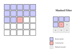
For image generation, PixelRNN [23] applies the autoregressive factorization to pixels, scanning the image in raster order (top to bottom, left to right): where each pixel takes values in (modeled via a softmax over 256 categories). PixelRNN uses LSTM layers to capture long-range dependencies along the raster scan. PixelCNN [24] replaces the recurrence with masked convolutions, convolutional filters that are zeroed out for “future” pixels, ensuring the autoregressive property.
Order-Agnostic Autoregressive Models and XLNet
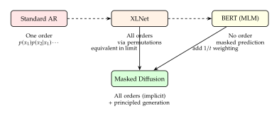
An important precursor to diffusion language models is the order-agnostic autoregressive model. XLNet [11] proposed training an autoregressive model over all possible permutations of the input sequence: where is the set of all permutations of . At each training step, a random permutation is sampled, and the model learns to predict each token given the preceding tokens in that permutation order.
This is significant because:
Unlike BERT, XLNet is a proper generative model: it can assign exact likelihoods to sequences.
Unlike standard AR models, it sees bidirectional context during training (through permuted orders).
The expected loss over all permutations gives equal weight to every possible conditioning pattern.
Remark 3.
We will see in Section Theoretical Results that absorbing discrete diffusion implicitly averages over all factorization orders, making it equivalent to XLNet's objective in the continuous-time limit. However, diffusion models achieve this through the elegant mechanism of masking and unmasking, without explicitly enumerating permutations. This connection was formally established by Ou et al. [2].
The following table summarizes the key properties of these model families:
| Property | AR | NADE/MADE | BERT | Diffusion |
| Generative model | Yes | Yes | No | Yes |
| Exact likelihood | Yes | Yes | No | Via ELBO |
| Bidirectional context | No | Via ensembles | Yes | Yes |
| Parallel generation | No | No | N/A | Yes |
| All factorization orders | No | Via orderings | N/A | Yes (implicit) |
| Iterative refinement | No | No | N/A | Yes |
Masked Language Modeling (BERT)
A different approach to modeling sequences, which will prove central to diffusion language models, is masked language modeling (MLM), introduced by BERT [3]. Rather than factoring the distribution autoregressively, BERT randomly masks a fraction of tokens (typically 15%) and trains a bidirectional Transformer to predict the masked tokens from the unmasked context:
BERT was originally designed as a representation learner, not a generative model. However, the connection between masking and diffusion turns out to be profound. As we will show in Section Masked Diffusion Language Models (MDLM), the training objective of masked diffusion language models is precisely a weighted average of MLM losses at different masking rates. BERT's MLM can be viewed as training a diffusion model at a single, fixed noise level.
Remark 4.
The connection between BERT and diffusion provides a surprising bridge: encoder-only models (BERT-style), traditionally used for understanding tasks, can be turned into principled generative models by simply modifying the training loss to weight different masking rates appropriately.
Recap: Diffusion Models for Images
We briefly recap the continuous diffusion framework for images, which forms the foundation for understanding the discrete extensions needed for language. This material is covered in detail in earlier chapters; here we highlight the aspects most relevant to the discrete setting.
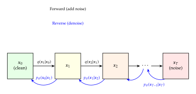
Forward Process (Adding Noise)
Given a data point , the forward process adds Gaussian noise over steps: where is a noise schedule. Defining and , the marginal at any time is available in closed form: (Continuous Forward Marginal) As with appropriate scheduling, and .
Reverse Process (Denoising)
The reverse process generates data by denoising: The true reverse posterior, conditioned on , is also Gaussian: where and are known functions of , , and the noise schedule.
Training Objective
The ELBO decomposes into a sum of KL divergences: With the -prediction parameterization, this simplifies to a reweighted MSE loss. For the -prediction parameterization (DDPM), the loss becomes:
Why Continuous Diffusion Does Not Directly Work for Language
Language tokens live in a discrete space . Adding Gaussian noise to a one-hot vector produces a continuous vector that no longer corresponds to any valid token. Several attempts have been made to apply continuous diffusion to text by embedding tokens into a continuous space [25][26], but these approaches face fundamental difficulties:
Embedding-space mismatch. Rounding a continuous diffusion output back to the nearest token embedding introduces errors that accumulate during sampling.
No natural metric. Unlike pixel values where nearby values are similar (pixel 128 is close to 129), tokens have no natural ordering or distance metric. The word “cat” is not “close to” “bat” in any meaningful geometric sense that Gaussian noise respects.
High dimensionality. Modern vocabularies have to tokens. Operating in this high-dimensional discrete space via continuous relaxations is wasteful.
Remark 5.
This difficulty motivates the development of discrete diffusion models, diffusion processes that operate directly on categorical variables, replacing Gaussian noise with structured corruption processes such as uniform noise or masking.
Discrete Diffusion: The D3PM Framework
The first principled framework for diffusion in discrete spaces was D3PM (Structured Denoising Diffusion Models in Discrete State-Spaces) [17]. D3PM generalizes DDPM to categorical data by replacing Gaussian transitions with categorical transitions defined by stochastic matrices.
Setup
Consider a single token , represented as a one-hot vector in . The forward process is a Markov chain defined by transition matrices , where entry .
Definition 1 (D3PM Forward Process).
The forward process corrupts data via: where is treated as a row vector and is a row-stochastic matrix (rows sum to 1).
The marginal at time given the initial data is computed via the cumulative product: (D3PM Marginal)
This is the discrete analogue of the Gaussian marginal . Just as controls how much of the original signal remains in continuous diffusion, controls how much of the original token identity is preserved.
Types of Transition Matrices
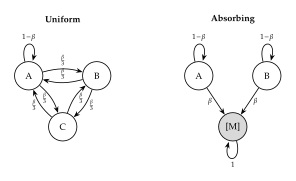
D3PM considers three types of transition matrices, each inducing a different corruption process:
1. Uniform Diffusion.
where is the all-ones vector. With probability the token is kept, and with probability it is resampled uniformly from all states. Reading this off the matrix, the token is retained with total probability and moves to each other state with probability , so every row sums to . The stationary distribution is uniform over all tokens.
2. Absorbing State Diffusion.
(Absorbing Transition) Tokens either stay the same or transition to a special absorbing state . Once masked, a token remains masked. The stationary distribution is a point mass on .
3. Discretized Gaussian Diffusion.
for some constant . This imposes ordinal structure: nearby states are more likely transitions. This is suitable for data with natural ordering, such as discretized pixel values.
Reverse Posterior
Using Bayes' theorem, the true reverse posterior (conditioned on knowing ) is: (D3PM Reverse Posterior) In categorical/matrix form: (D3PM Reverse Categorical) where denotes the elementwise (Hadamard) product. This is the discrete analogue of the Gaussian posterior in continuous DDPM.
-Parameterization and Training
The model learns using the -parameterization: a neural network predicts a distribution over clean data , and then the reverse transition is computed by plugging this prediction into the Bayes posterior: (D3PM X0 Param)
The training objective is the variational bound (VB) on the negative log-likelihood. Every term below is non-negative, so : it is the negated ELBO, and it is minimised. (D3PM VLB)
Since all distributions are categorical, the KL divergences have closed-form expressions:
Remark 6.
Austin et al. found that training with the variational bound alone can be unstable. They propose an auxiliary cross-entropy loss: which directly encourages the network to predict accurately from any noisy . The total loss is .
Algorithm 1: D3PM Training.
Masked Diffusion Language Models (MDLM)
While D3PM provides a general framework for discrete diffusion, it was MDLM (Simple and Effective Masked Diffusion Language Models) [18] that demonstrated that a careful specialization to the absorbing state (masking) process, combined with a simplified training objective, could dramatically close the gap with autoregressive models. MDLM was published at NeurIPS 2024 and represents a key turning point for the field.
Forward Process: Masking
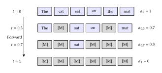
MDLM focuses exclusively on absorbing-state diffusion. For a sequence , each token is independently either kept or masked: (MDLM Forward) where is the one-hot vector for the token, is a decreasing noise schedule with (no masking) and (fully masked), and is continuous time.
In words: at time , each token independently survives with probability or is masked with probability .
Simplified Reverse Posterior
For absorbing-state diffusion, the reverse posterior simplifies dramatically compared to the general D3PM case: (MDLM Reverse Posterior) for .
Remark 7 (Key structural property).
If a token is not masked at time , it deterministically stays the same at time . Only masked tokens have non-trivial reverse transitions. This is the “carry-over” property: once unmasked, always unmasked.
The SUBS Parameterization
The learned reverse process substitutes the neural network prediction for the true : Two structural constraints are imposed on the network output:
Zero masking probability: The network never predicts as a clean token: . In practice, the logit for is set to before the softmax.
Carry-over unmasking: If , the output simply copies the input: .
Rao-Blackwellized Training Objective
The main contribution of MDLM is a dramatically simplified training objective obtained by analytically computing expectations (Rao-Blackwellization). Starting from the D3PM-style ELBO with complex KL divergences, the carry-over and zero-masking constraints allow the diffusion loss to simplify to:
Theorem 1 (MDLM Discrete-Time Loss).
The discrete-time Rao-Blackwellized diffusion loss is: (MDLM Discrete LOSS) where the inner product is the predicted probability of the true token at position , and the weight depends on the noise schedule. Since and is decreasing, that weight is non-negative, and so is each : the whole expression is a non-negative quantity to be minimised.
This is simply a weighted cross-entropy loss evaluated only at masked positions. Compared to the D3PM parameterization, this has lower variance because expectations are computed analytically rather than estimated via sampling.
Continuous-Time Limit
Taking , the discrete sum becomes an integral:
Theorem 2 (MDLM Continuous-Time NELBO).
The continuous-time negative ELBO is: (MDLM Continuous LOSS) where is the derivative of the noise schedule. Because decreases, and the weight is positive; for the linear schedule it is exactly .
Noise Schedule Invariance
A remarkable property emerges through the change of variables : (MDLM Schedule Invariant)
Proposition 1 (Schedule Invariance).
This eliminates one degree of hyperparameter freedom: any monotone schedule running from down to converges to the same objective, since those are exactly the conditions under which sweeps the full range .
Connection to Masked Language Modeling
For a sequence of length , the MDLM objective can be written as: At each time , the masking rate is , and the loss is the cross-entropy of predicting masked tokens, which is precisely masked language modeling (MLM) at that masking rate. The integral averages over all masking rates from 0 to 1, weighted by .
Remark 8.
MDLM training is a weighted average of MLM losses across different masking rates. This provides a formal bridge: BERT [3] performs MLM at a single fixed masking rate (15%), while MDLM averages over all masking rates with principled weighting. This endows encoder-only models with generation capability without sacrificing their representation quality.

Score Entropy Discrete Diffusion (SEDD)
An alternative approach to discrete diffusion, developed concurrently with MDLM, is SEDD (Score Entropy Discrete Diffusion) [19], which won the ICML 2024 Best Paper award. Instead of parameterizing the reverse process directly, SEDD learns ratios of probabilities, the discrete analogue of the score function.
The Concrete Score
In continuous diffusion, the score is the key object. In discrete spaces, there are no gradients. SEDD defines the concrete score as the ratio: for states that are “neighbors” of (differing at a single position). This is the discrete analogue of the Stein score, since: A key advantage is that normalizing constants cancel in ratios:
Continuous-Time Markov Chain (CTMC)
SEDD operates in continuous time. The forward process is governed by a rate matrix :
For absorbing diffusion, the rate matrix is: where is the rate of masking. Each non-mask token transitions to at rate . Note that is a row vector and acts on the right, so that the generator axioms hold in the usual orientation: off-diagonal entries are non-negative and every row of sums to zero, which is what conserves total probability.
Score Entropy Loss
The score entropy loss for estimating the concrete score is: (Score Entropy) where denotes neighbors of , are the transition rates of the forward process, and (Score Entropy Normalizer) is the normalizing term that makes the per-neighbour loss bottom out at exactly zero. Writing , we have , which vanishes only at ; on the positive ray, so is strictly convex there; and . Hence:
Convex in , ensuring stable optimization.
Non-negative, equaling zero if and only if .
The discrete analogue of the Fisher divergence used in continuous score matching.
Remark 9.
For absorbing diffusion, the concrete score factorizes into a time-dependent scalar times the conditional distribution of clean data: This connects SEDD directly to masked language modeling: the learned score is essentially predicting the clean token distribution, scaled by a known time-dependent factor. Since (Section The Continuous-Time Markov Chain Perspective), that scalar is , which is the same quantity that appears in the MDLM reverse posterior; the two remarks are one statement in two notations.
Detailed Derivation: From D3PM to MDLM
The transition from D3PM to MDLM involves several mathematical simplifications that are instructive to derive in full detail. We walk through each step, starting from the general D3PM ELBO and arriving at the clean MDLM objective.
Step 1: Specializing to the Absorbing Process
Recall from the general D3PM framework that the reverse posterior is given by . For the absorbing transition matrix , the cumulative product has a particularly clean form. For a single token: Since each step either keeps the token (with probability ) or masks it (with probability ), the probability that a token survives to time is: The marginal is then: (Absorbing Marginal) This is exactly the MDLM forward process written in discrete time.
Step 2: Computing the Reverse Posterior Explicitly
We now derive from first principles. Using Bayes' theorem:
Case 1: .
If is a real token (not masked), then (the only way a real token appears at time is if it was never masked). In this case, must also equal : The one-line Bayes check: the numerator is and the denominator is , so the ratio is 1; the competing candidate has numerator , because the mask is absorbing. This is the “carry-over” property: unmasked tokens remain fixed.
Case 2: .
We need to compute: The first numerator factor is a one-step transition and the second is a marginal given ; below we keep both time indices explicit so the two are never confused.
Sub-case 2a: (token was unmasked at , then masked at ).
Since , we have , so: (Posterior Unmask)
Sub-case 2b: (token was already masked at ).
(Posterior Staymask)
We can verify these sum to 1:
Combining both cases yields exactly .
Step 3: From KL Divergence to Cross-Entropy
The D3PM variational bound contains terms of the form:
For the absorbing process, when , both the true and learned reverse posteriors are deterministic (keeping unchanged), so the KL is zero. The non-trivial contribution comes only from :
With the SUBS parameterization and the zero-masking-probability constraint, the reverse distribution at a masked position takes the form: where is the network's predicted probability for token .
The KL divergence between the true and learned posteriors at a masked position can be expanded:
This is the Rao-Blackwellization: the KL divergence at masked positions reduces to a weighted negative log-probability of the true token. The weighting is exactly the coefficient in the MDLM loss .
Step 4: Summing Over Positions and Time
For a sequence of length with independent masking, summing over all positions and time steps:
Taking and using (where ): Since is decreasing, , so and the weight is positive. This recovers the MDLM continuous-time NELBO .
Step 5: The Change of Variables to Schedule Invariance
The schedule invariance result follows from the substitution , which yields . The integral becomes:
The key observation is that absorbs the entire schedule-dependent weighting, leaving an integral that depends only on the masking probability (since ). Two different schedules and that sweep through the same range of masking probabilities will produce the same integral, just traversed at different speeds. (Here names a second schedule; the prime continues to mean throughout.)
Remark 10.
This schedule invariance is unique to the continuous-time limit. In practice with finite , the schedule affects training dynamics and variance. Linear (), cosine, and geometric schedules all converge to similar final performance but may train at different speeds.
Worked Example: MDLM on a 3-Token Vocabulary
To make these derivations concrete, consider a toy example with two real tokens, , so , plus the extra state, giving three states per position; the sequence length is . (Throughout this chapter counts the real vocabulary, and is an additional state appended to it.)
Example 1.
Let and suppose (linear schedule). At time :
Each token is masked independently with probability .
Possible states of : with prob ; with prob ; with prob ; with prob .
Consider the state . The model must predict the first token. The training loss contribution for this state at this time is:
Notice the weight , against at . The weight is not a preference for easy examples: it exactly cancels the number of terms being summed. At masking rate the expected number of masked positions is , so the expected contribution of that rate is , the same at every . Integrating over gives for any schedule running from 1 down to 0. The is what makes the measure over masking rates uniform; it is the reason MDLM is an average of MLM losses rather than a reweighting of them.
The Continuous-Time Markov Chain Perspective
The discrete-time formulations of D3PM and MDLM have natural continuous-time analogues via continuous-time Markov chains (CTMCs). This perspective, developed in Campbell et al. [27] and refined in SEDD [19], provides elegant theoretical properties and connects discrete diffusion to the score-based framework.
Rate Matrices and the Master Equation
A CTMC over a finite state space is characterized by a rate matrix (or generator) , where:
for (transition rate from state to state )
(rows sum to zero)
The probability distribution evolves according to the master equation (Kolmogorov forward equation): (Master Equation)
This is the discrete-space analogue of the Fokker-Planck equation in continuous diffusion. The solution is: where the matrix exponential gives the transition probability matrix.
The Absorbing Rate Matrix
For masked diffusion, the rate matrix is: (Absorbing RATE) where controls the masking rate.
In matrix form, for a 3-state system :
The masking probability at time is: Comparing with MDLM's : we have , or equivalently .
The Reverse CTMC
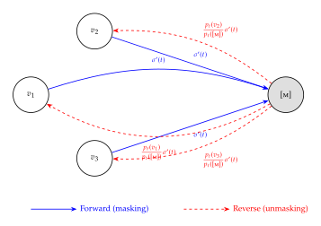
The time-reversed CTMC has rate matrix: (Reverse RATE) This is the discrete analogue of Anderson's reverse-time SDE. The ratio is exactly the concrete score, which SEDD learns to estimate.
For the absorbing process, the reverse rate simplifies: the only non-trivial transitions are from to real tokens, with rate:
Remark 11.
This reveals why MDLM and SEDD are closely related: MDLM directly parameterizes (the conditional clean distribution), while SEDD parameterizes (the concrete score). For absorbing diffusion, these are related by a known time-dependent factor:
Large Language Diffusion Models (LLaDA)
With the theoretical foundations from MDLM and SEDD, the next question was: can masked diffusion models scale to the size and capability of modern LLMs? LLaDA (Large Language Diffusion Models) [5] provided a resounding “yes,” demonstrating that an 8-billion parameter diffusion model can match or exceed autoregressive models on many benchmarks.
Core Thesis
LLaDA challenges the prevailing assumption that autoregressive formulations are necessary for emergent LLM capabilities such as in-context learning, instruction following, and chain-of-thought reasoning. The authors argue that these capabilities arise from the interplay between Transformers, model scale, data scale, and Fisher consistency, a statistical property guaranteeing that the model can recover the true data distribution with sufficient data and capacity, rather than from the left-to-right factorization specifically.
Definition 2 (Fisher Consistency).
A generative model family is Fisher consistent for a data distribution if, given infinite data and a sufficiently expressive network: Both autoregressive models and masked diffusion models satisfy this property.
Forward and Reverse Process
LLaDA uses the same masking-based forward process as MDLM, but with a clearer presentation in terms of continuous time :
Forward process (token-level):
(Llada Forward) At , no tokens are masked; at , all tokens are masked. This is the simplest possible masking schedule: .
Reverse process (token-level):
For , the reverse transition has four cases: (Llada Reverse)
Remark 12 (Time-Free Parameterization).
A crucial insight from LLaDA: the optimal predictor depends only on which tokens are visible, not on the timestep . This means the mask predictor does not need time as an input, a significant simplification.
Training Objective
The LLaDA training loss is: (Llada LOSS)
The weighting is theoretically motivated: it ensures that the loss is a valid upper bound on the negative log-likelihood:
Remark 13.
This weighting distinguishes LLaDA from MaskGIT [4], which omits this term and thus lacks a principled maximum-likelihood foundation. The per-token weight is larger at small , but the expected number of masked positions at rate is , so the expected contribution of each rate is : the weighting makes the measure over masking rates exactly uniform. That is precisely what turns a masked language model trained at one rate into a likelihood-based generative model.
Architecture
LLaDA 8B uses essentially the same Transformer architecture as LLaMA 3 8B. One design decision differs, and the table below shows it together with the consequence that follows from it:
| Feature | LLaDA 8B | LLaMA3 8B |
| Attention | Full bidirectional | Causal (left-to-right) |
| KV cache | Not applicable | Used for fast inference |
| Positional encoding | RoPE | RoPE |
| Normalization | RMSNorm | RMSNorm |
| Activation | SwiGLU | SwiGLU |
| Parameters | 8B | 8B |
The key architectural change is removing the causal attention mask, allowing the model to attend to all positions bidirectionally. This is essential for the diffusion formulation, where the model needs to use both left and right context to predict masked tokens. However, it means that the KV cache optimization, crucial for fast autoregressive inference, is not directly applicable.
Supervised Fine-Tuning for Diffusion Models
For instruction following, LLaDA uses a modified SFT loss where only the response tokens are subject to masking: (Llada SFT) where are the prompt tokens (always unmasked), are the response tokens (subject to masking), and is the response length.
Experimental Results: How Good Are Diffusion Language Models?
Before describing the sampling algorithms, let us examine the empirical evidence for diffusion language models to understand how they compare with autoregressive models across various tasks.
Language Modeling Perplexity (MDLM)
MDLM [18] provides the first strong evidence that masked diffusion can approach autoregressive performance. On the One Billion Word benchmark (LM1B) with 110M parameter models:
| Model | Type | Perplexity () |
| Transformer (AR, retrained) | Autoregressive | 20.86 |
| BERT-Mouth | MLM generation | |
| D3PM (absorbing) | Discrete diffusion | |
| DiffusionBERT | Discrete diffusion | |
| SEDD | Score-based discrete | |
| MDLM | Masked diffusion |
MDLM achieves a 17% improvement over SEDD (the prior best diffusion model) and comes within 10% of the AR baseline. The progression from D3PM () to MDLM () demonstrates the power of the simplified Rao-Blackwellized objective.
Benchmark Results at Scale (LLaDA 8B)
LLaDA 8B [5], trained on 2.3 trillion tokens, provides the first comparison of diffusion models with modern LLMs at the 8B parameter scale:
| Benchmark | LLaDA 8B | LLaMA3 8B | LLaMA2 7B |
| (2.3T tokens) | (15T tokens) | (2T tokens) | |
| MMLU | 65.9 | 65.4 | 45.9 |
| GSM8K | 70.7 | 53.1 | 14.3 |
| MATH | 27.3 | 15.1 | 3.2 |
| HumanEval | 33.5 | 34.2 | 12.8 |
| HumanEval-FIM | 73.8 | 73.3 | 26.9 |
| HellaSwag | 72.5 | 79.1 | 76.0 |
| WinoGrande | 74.8 | 77.3 | 72.5 |
The largest margins are on mathematics (GSM8K: 70.7 vs. 53.1; MATH: 27.3 vs. 15.1), obtained with 2.3T training tokens against LLaMA3's 15T. This suggests that the bidirectional architecture may have advantages for mathematical reasoning, while the commonsense benchmarks, where LLaDA trails, suggest the advantage is not uniform across task types.
Post-SFT Performance
After supervised fine-tuning, LLaDA 8B Instruct (using only SFT, no RLHF/DPO) achieves:
| Benchmark | LLaDA 8B Instruct |
| MMLU | 65.5 |
| ARC-C | 88.5 |
| HumanEval | 49.4 |
| GSM8K | 78.6 |
| MATH | 26.6 |
These results are competitive with AR models that use RLHF alignment, suggesting that the diffusion training paradigm provides strong instruction-following capabilities even without explicit preference optimization.
Representation Quality (MDLM on GLUE)
A key question is whether the diffusion training objective degrades the representation quality of encoder-only models. MDLM tests this by fine-tuning a BERT model with the MDLM objective and evaluating on GLUE:
| Task | AR | BERT | BERT+MDLM |
| MNLI (m/mm) | 80.9/80.8 | 84.4/85.4 | 84.8/85.1 |
| QQP (F1) | 87.0 | 88.4 | 88.5 |
| SST-2 | 90.1 | 92.2 | 92.2 |
| CoLA | 33.4 | 54.8 | 57.7 |
| Average | 74.9 | 81.6 | 82.1 |
Fine-tuning BERT with the MDLM objective does not degrade representation quality; it actually slightly improves it (82.1 vs. 81.6 average) while adding generative capabilities. This demonstrates that diffusion training and representation learning are compatible.
Scaling Laws for Diffusion Language Models
LLaDA demonstrates that diffusion language models exhibit scaling behavior comparable to autoregressive models. Testing across FLOPs from to on six benchmarks, diffusion models follow the same general scaling trend as ARMs.
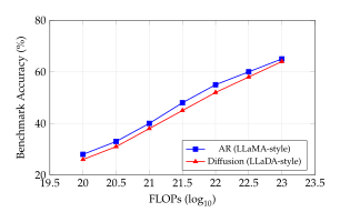
An important finding from the scaling experiments is that likelihood metrics alone are insufficient predictors of downstream task performance for diffusion models. This contrasts with AR models, where lower perplexity reliably predicts better downstream performance. For diffusion models, the ELBO (which is an upper bound on negative log-likelihood) does not always correlate with task-specific metrics, suggesting that evaluation strategies for diffusion models need further development.
Sampling Algorithms and Remasking Strategies
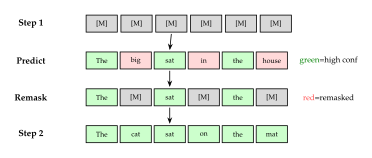
Generation in diffusion language models works by iteratively unmasking tokens. Starting from a fully masked sequence , the model progressively reveals tokens over steps. The key design choice is the remasking strategy: after the model predicts all masked tokens, which predictions should be kept and which should be re-masked for refinement?
Random Remasking
The simplest approach randomly selects which tokens to remask:
Algorithm 2: Sampling with Random Remasking (LLaDA).
[t]
- Input: Mask predictor , prompt , response length , steps
- Initialize Fully masked
- for
- ,
- Predict all masked positions
- if
- Randomly remask of the predicted tokens so stand committed
- result
- return
Low-Confidence Remasking
A more effective strategy is to remask the tokens that the model is least confident about:
Algorithm 3: Sampling with Low-Confidence Remasking (LLaDA).
[t]
- Input: Mask predictor , prompt , response length , steps
- Initialize
- for
- ,
- for each masked position
- Predict and compute confidence
- Cumulative number committed by step
- New commitments this step, with
- Commit the highest-confidence predictions among the currently masked positions; remask the rest
- result
- return
Remark 14.
Note that counts all positions committed so far, not the ones committed on this step; the per-step count is the difference . Applying to the masked-only pool would over-commit early and finish before step : at , it commits 3 then 6, exhausting the sequence at step two of three, whereas the cumulative reading gives the intended 3, 3, 3.
Low-confidence remasking is the default strategy in LLaDA and consistently outperforms random remasking. The intuition is clear: by keeping the most confident predictions and re-predicting the uncertain ones with additional context from the newly revealed tokens, the model iteratively refines its output.
Block Diffusion: Semi-Autoregressive Generation
Block diffusion [6] interpolates between fully parallel diffusion and fully sequential autoregressive generation. The sequence is divided into blocks, and blocks are generated left-to-right (autoregressively), while tokens within each block are generated via diffusion (in parallel).
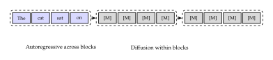
Write for the block size, so a sequence of length is divided into blocks and block is conditioned on all earlier blocks . The block diffusion loss is: with the same positive weight as before, equal to on the linear schedule. Every factor is non-negative.
The block size controls the trade-off:
: fully autoregressive, blocks, one token committed per pass
: fully diffusion-based, a single block
: semi-autoregressive, blocks, at most positions committed per pass, and tokens of frozen prefix before the last block
Remark 15.
The mechanism, rather than any single benchmark number, is the point: shrinking buys each prediction more committed left context at the cost of more sequential passes, and growing trades that context away for parallelism. The autoregressive and fully-parallel samplers are the two endpoints of one dial [6].
Detailed Analysis of Masking Schedules
The masking schedule determines how quickly tokens are corrupted during the forward process. While the continuous-time NELBO is schedule-invariant at convergence, the schedule significantly affects training dynamics, variance, and finite-step sampling quality.
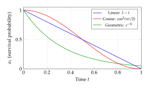
Common Schedules
Linear Schedule.
for . This is the simplest choice and is used in LLaDA. The masking rate increases linearly, and the weight diverges as (few tokens masked), placing heavy emphasis on near-complete sequences.
Cosine Schedule.
. Inspired by the cosine schedule for continuous diffusion [28], this provides the smoothest start, masking very slowly for small and then, past the midpoint, more aggressively than the linear schedule (at , against the linear ):
Geometric (Exponential) Schedule.
for some rate parameter :
Effect on Training Variance
At each training step, we sample a time and compute the loss at that masking level. The variance of the gradient estimator depends on the schedule through the weight :
When varies widely, the gradient estimator has high variance.
The linear schedule has , which diverges as , leading to occasionally very large gradients when a nearly-complete sequence is sampled.
Low-discrepancy time sampling (e.g., stratified sampling of ) can reduce this variance significantly [7].
Mask Ratio Bandwidth
LLaDA 2.0 introduces mask ratio bandwidth: clipping the noise schedule to instead of , which avoids the extreme masking rates that cause high variance: This clips the masking level rather than the time: it is an affine rescaling of , which corresponds to a restriction of to a subinterval only for the linear schedule. For the cosine schedule with , the induced reparametrisation departs from the affine prediction by up to in .
Training Algorithms in Detail
We present the complete training algorithms for both pre-training and supervised fine-tuning of diffusion language models.
Algorithm 4: MDLM / LLaDA Pre-Training.
[t]
- Input: Bidirectional Transformer , data distribution , schedule
- repeat
- Sample sequence
- Sample time
- for each position Independent masking
- With probability : set
- Otherwise: set
- Forward pass: compute for all Single forward pass
- Compute loss:
- Update via gradient descent on
- until converged
Algorithm 5: Diffusion Language Model SFT (Instruction Tuning).
[t]
- Input: Pre-trained , prompt-response pairs
- repeat
- Sample
- Sample
- for each response position Only mask response
- With probability : set
- Otherwise: set
- Concatenate: Prompt always visible
- Forward pass: compute for all masked positions
- Compute loss:
- Update
- until converged
Remark 16 (Comparison with AR SFT).
In autoregressive SFT, the prompt tokens are processed via teacher forcing (the model sees the prompt and predicts the response left-to-right). In diffusion SFT, the prompt is simply concatenated as unmasked context, and no architectural change is needed. The prompt is always fully visible, and the response is the only part subject to masking and prediction.
Detailed Sampling Procedures
We present the complete sampling algorithms, including the newly introduced ancestral sampling variant and the semi-autoregressive extension.
Ancestral Sampling (Principled but Slow)
The most principled sampling method follows the learned reverse process exactly:
Algorithm 6: Ancestral Sampling for Masked Diffusion.
[H]
- Input: Trained model , response length , number of steps
- Initialize
- for
- ,
- Compute for all masked positions Forward pass
- for each position
- if
- With probability : keep Stay masked
- With probability : sample Unmask
- else
- Carry over (already unmasked)
- return
At each step, each masked token either stays masked (with probability ) or is unmasked by sampling from the predicted distribution. This follows the exact reverse posterior .
Caching Optimization
When no new tokens are unmasked in a step (which can happen, especially with few remaining masked tokens), the forward pass can be skipped entirely. Furthermore, if the model does not use time conditioning (as suggested by Remark 12), consecutive steps with the same set of unmasked tokens produce identical predictions, so those passes can be reused. How much this saves depends entirely on the sampler and the schedule: it is the fraction of steps that commit nothing.
Semi-Autoregressive (SAR) Generation
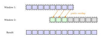
For sequences longer than the context window , MDLM introduces a sliding-window approach:
Algorithm 7: Semi-Autoregressive Generation (MDLM).
[H]
- Input: Model , context window , prefix overlap , total length
- Generate initial window via standard reverse diffusion
- while
- Last tokens as fixed prefix
- Initialize new window:
- Generate via reverse diffusion with prefix fixed (carry-over ensures prefix stays)
- Append the newly generated tokens (positions through of the new window) to output
- Slide window forward
- return output After windows,
Advantages over Autoregressive LLMs
Diffusion language models offer several structural advantages over their autoregressive counterparts. These advantages are not merely theoretical; they have been demonstrated empirically in recent large-scale models.
Parallel Generation
The most obvious advantage is parallelism. In autoregressive generation, producing tokens requires serial forward passes, each of which reads the full KV cache but produces only a single token. This makes AR inference memory-bandwidth bound on modern GPUs, leading to poor hardware utilization.
Diffusion models, in contrast, process and refine all tokens simultaneously in each denoising step. If the model requires denoising steps (typically ), the total number of forward passes is rather than . Each forward pass has much higher arithmetic intensity (ratio of compute to memory operations), better saturating modern GPU compute units.
Example 2.
Mercury Coder achieves 1,109 tokens/second on H100 GPUs, compared to approximately 60–200 tokens/second for comparable autoregressive models. This represents a 5–10 speedup, achieved purely through the diffusion generation paradigm [8].
Bidirectionality and the Reversal Curse
Autoregressive models factor the distribution left-to-right, which creates a fundamental asymmetry. If trained on “A is B,” the model learns but not . This is the reversal curse [1].
Diffusion language models are inherently bidirectional: they use full attention (no causal mask), conditioning on both left and right context simultaneously. This means they naturally learn both directions.
Example 3 (Reversal Curse Experiment from LLaDA).
On Chinese poem completion (given first half, complete second half vs. given second half, complete first half):
| Model | Forward | Reversal |
| GPT-4o | 82.7% | 34.3% |
| Qwen2.5 7B | 75.9% | 38.0% |
| LLaDA 8B | 48.8% | 42.4% |
Native Fill-in-the-Middle
Because diffusion models condition bidirectionally, fill-in-the-middle (FIM) is natively supported without special training modifications. Given a prefix and suffix, the model can generate the middle by treating the prefix and suffix as unmasked context and the middle as the masked region to be diffused.
LLaDA achieves 73.8% on HumanEval-FIM versus LLaMA3's 73.3%, despite LLaMA3 requiring specific FIM training.
Iterative Refinement and Error Correction
Perhaps the most intriguing advantage is the ability to self-correct. In autoregressive generation, once a token is emitted, it cannot be changed. An early mistake propagates through the entire remaining sequence. Diffusion models, through the remasking mechanism, can revisit and revise earlier decisions.
In low-confidence remasking (Algorithm alg:confidence_remasking), the model naturally identifies positions where it is uncertain and re-predicts them with additional context. This provides a built-in form of error correction that autoregressive models lack.
Remark 17 (Fault Tolerance).
In settings where early tokens may be corrupted (e.g., noisy inputs, adversarial prompts), diffusion models are more robust because they can use the full bidirectional context, including later, uncorrupted tokens, to correct earlier errors. Autoregressive models, processing left-to-right, cannot look ahead to verify consistency.
Flexible Generation Order
Autoregressive models are committed to a single generation order (left-to-right). Diffusion models can generate tokens in any order; the order is determined dynamically by the confidence scores and remasking strategy. This flexibility allows the model to:
Generate high-certainty tokens first (e.g., function signatures before implementations).
Fill in details after establishing the overall structure.
Naturally handle tasks like code completion where the generation order is not left-to-right.
Classifier-Free Guidance for Diffusion Language Models
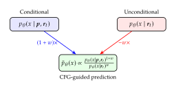
Classifier-free guidance (CFG) [29], a technique that dramatically improves conditional generation quality in image diffusion models, can also be applied to diffusion language models.
CFG for Conditional Text Generation
In the image domain, CFG interpolates between conditional and unconditional predictions: where is the guidance strength and is the condition (e.g., text prompt).
For masked diffusion language models, the analogous formulation operates on the predicted token logits. Given a prompt and a masked response , the guided logits are: where are the conditional logits (with prompt) and are the unconditional logits (prompt replaced with masks or dropped).
Remark 18.
LLaDA reports that CFG “consistently benefits” conditional generation quality, but disables it in the main results for fair comparison with AR models. The ability to trade off diversity for quality via a guidance parameter is a unique advantage of the diffusion framework.
Comparison with AR Temperature Scaling
In autoregressive models, the analogue of CFG is temperature scaling: where sharpens the distribution (more deterministic) and flattens it (more diverse).
CFG in diffusion models is more powerful than simple temperature scaling because it leverages the difference between conditional and unconditional predictions, which captures information about what the prompt specifically requests. Temperature scaling merely adjusts the sharpness without such semantic grounding.
Challenges: Generation Speed and What Makes It Slow
Despite the advantages, diffusion language models face significant challenges related to generation speed and efficiency. Understanding these challenges is crucial for appreciating the engineering innovations in models like Mercury and LLaDA 2.0.
The Cost of Multiple Denoising Steps
While diffusion models process all tokens in parallel per step, they require multiple denoising steps (typically 16–256) to generate high-quality output. Each step involves a full forward pass through the Transformer. If the model uses steps and the autoregressive model generates tokens:
AR model: 512 forward passes, each producing 1 token (but using efficient KV cache)
Diffusion model: 64 forward passes, each processing all 512 tokens
The AR model benefits enormously from the KV cache: after the first pass, each subsequent pass only processes a single new token, reusing cached key-value pairs. The diffusion model must process the full sequence at each step, because unmasking changes the content of already-processed positions and so invalidates any cached keys and values, making each individual forward pass much more expensive.
No KV Cache
The fundamental incompatibility between bidirectional attention and the KV cache is the single biggest efficiency challenge:
AR models with KV cache: After the prefill phase, each token generation requires attention computation proportional to (attending to all cached tokens), but the computation is done only for the new token.
Diffusion models: Each denoising step requires full self-attention over all tokens, with cost , simply because there are queries rather than one. What the masking breaks is not the attention pattern, which is the same complete pattern at every step, but the cache: unmasking rewrites the token content at positions whose keys and values were already computed, so the stored and no longer describe those positions and must be recomputed.
Quality-Speed Trade-off
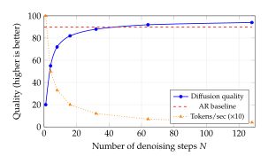
The number of denoising steps directly controls the trade-off between generation quality and speed:
More steps: better quality (more refinement iterations), slower generation.
Fewer steps: faster generation, but tokens may not be sufficiently refined.
Finding the optimal is an active research challenge. LLaDA shows that results are relatively insensitive to within a reasonable range, but extremely few steps (e.g., ) significantly degrade quality.
Arithmetic Intensity Analysis
To understand the speed difference between AR and diffusion models quantitatively, consider the arithmetic intensity (AI), the ratio of floating-point operations to bytes transferred from memory:
AR inference (generation phase).
After the prefill, each token generation step involves:
Reading the model weights: bytes per layer. For a model with parameters in
bf16this is bytes, and it is the dominant transfer.Reading the KV cache: bytes, smaller than the weight read at typical and .
Computing one token against those weights: FLOPs.
AI FLOP per byte at batch size one, independent of model size: memory-bandwidth bound.
Diffusion inference (each denoising step).
Each step involves:
Reading model weights: bytes (same as AR)
Computing attention for query tokens: FLOPs
AI , compute bound for long sequences
The key insight is that diffusion inference has higher arithmetic intensity than AR generation-phase inference. An H100 SXM5 delivers 3.35,TB/s of HBM3 bandwidth against a dense bf16 tensor-core peak of 989.5,TFLOP/s, so the ridge point, where the machine stops being bandwidth bound and starts being compute bound, is
AR generation sits at AI , which reaches of peak: over 99% of the compute is idle. Even at AI only 3.4% of peak is used. Diffusion inference can reach AI , which for in the hundreds crosses the ridge and puts the machine on the compute roof instead.
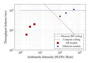
bf16. Converting the attainable rate to tokens per second requires dividing by the FLOPs per token, which is done separately in the text.Speculative Decoding and Fast Inference
Several techniques have been developed to accelerate diffusion language model inference, drawing inspiration from both the diffusion model literature and the autoregressive speculative decoding paradigm.
Confidence-Aware Parallel (CAP) Decoding
Introduced in LLaDA 2.0 [20], CAP training adds an auxiliary confidence loss that minimizes entropy selectively on correctly predicted tokens: The confidence loss sharpens the model's probability distributions for tokens it can predict well, enabling more tokens to be unmasked in a single step. This effectively reduces the required number of denoising steps while maintaining accuracy.
With CAP training, LLaDA 2.0-flash achieves 535 tokens/second, a 2.1 speedup over comparable AR baselines at 237–256 tokens/second.
Adaptive Step Count
Mercury [8] uses a dynamic step count that adjusts based on output complexity:
Simple structured outputs: 8 denoising steps
Complex reasoning: 16–20 denoising steps
This allows the system to automatically navigate the speed/quality trade-off without manual tuning.
Speculative Decoding for Diffusion
In autoregressive models, speculative decoding uses a small “draft” model to propose multiple tokens in parallel, which are then verified by the large model. An analogous approach for diffusion models:
A fast, small diffusion model generates a draft sequence in few steps.
The large model refines the draft in one or two additional denoising steps.
The refinement step leverages the bidirectional context to correct errors in the draft.
This naturally fits the diffusion paradigm because the refinement step is exactly what the model already does: denoising a partially correct sequence is a special case of denoising a partially masked sequence.
Scaling Up: LLaDA 2.0 and Mercury
The most recent frontier has been scaling diffusion language models to compete with state-of-the-art LLMs. Two prominent efforts are LLaDA 2.0 and Mercury.
LLaDA 2.0: From 8B to 100B via AR Conversion
LLaDA 2.0 [20] introduces a key insight: rather than training diffusion language models from scratch (which faces a maturity gap in data and infrastructure compared to AR models), convert pre-trained AR models into diffusion models.
Three-Phase Block-Level Training.
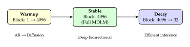
The conversion uses a Warmup-Stable-Decay (WSD) scheme:
Warmup: Progressively increase the block size from 1 (fully AR) to 4096 (full sequence MDLM): .
Stable: Full-sequence MDLM training at block size 4096 for deep bidirectional understanding.
Decay: Gradually reduce block size from 4096 back to 32 for efficient inference.
Mixture-of-Experts Architecture.
LLaDA 2.0 uses MoE (Mixture-of-Experts) architectures:
| LLaDA 2.0-mini | LLaDA 2.0-flash | |
| Total parameters | 16B | 100B |
| Active parameters | 1.4B | 6.1B |
| Layers | 20 | 32 |
| Experts | 256 routed + 1 shared | 256 routed + 1 shared |
| Context length | 32,768 | 32,768 |
Post-Training Pipeline.
LLaDA 2.0 introduces several innovations for post-training:
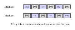
Complementary masking: Generates two antithetical training instances from a single sequence: one uses a random mask, the other its logical inverse. Every token appears unmasked exactly once per pair, doubling effective data utilization.
Mask ratio bandwidth: Clips the noise schedule to instead of , avoiding extreme masking rates that induce high gradient variance.
DPO for diffusion: Adapts Direct Preference Optimization using the ELBO as a surrogate for the intractable log-likelihood: where is the difference in ELBO between the current and reference model.
Results.
LLaDA 2.0-flash (100B total, 6.1B active) achieves an overall average of 73.18 across 47 benchmarks, competitive with Qwen3-30B (73.60) and its AR base model Ling-flash-2.0 (72.15). Notable strengths include:
HumanEval: 94.51% (vs. 93.29% for Qwen3-30B)
MBPP: 88.29% (vs. 86.65% for Qwen3-30B)
AIME 2025: 60.00% (competitive with 61.88%)
Mercury: Ultra-Fast Commercial-Scale Diffusion
Mercury [8] from Inception Labs represents the first commercial-scale diffusion language model, designed for maximum throughput.
Architecture.
Mercury uses a standard Transformer architecture; the key difference is the training loss (diffusion denoising instead of next-token prediction) and the generation algorithm (iterative denoising instead of sequential sampling). The architecture choice is explicitly stated to be “orthogonal to the fact that Mercury models are diffusion-based.”
Key Speed Results.
| Model | Speed (tok/s) | HumanEval |
| Mercury Coder Mini | 1,109 | 88.0% |
| Mercury Coder Small | 737 | 90.0% |
| Claude 3.5 Haiku | 61 | 86.0% |
| GPT-4o Mini | 59 | 88.0% |
| Gemini 2.0 Flash Lite | 201 | 90.0% |
Mercury Coder Mini is approximately 5–18 faster than comparable models while maintaining competitive quality.
Why So Fast?
The fundamental advantage comes from the diffusion generation paradigm:
Higher arithmetic intensity: Each denoising step processes many tokens in parallel, better saturating GPU compute units.
Fewer total forward passes: Even with 10 denoising steps for 100 tokens, that is 10 fewer forward passes than AR.
Proprietary inference engine: Custom kernels optimized for parallel denoising workloads with dynamically batched sampling.
Theoretical Results
The theoretical understanding of discrete diffusion has advanced significantly alongside the empirical progress. We survey key results that provide convergence guarantees and illuminate the connections between discrete and continuous diffusion.
Convergence Bounds for Discrete Diffusion
Theorem 3 (Convergence via Uniformization, Chen et al. 2024 [9]).
For absorbing-state discrete diffusion with vocabulary size and sequence length , using the uniformization-based exact sampler (no discretization error): where is the time horizon and is the score estimation error. Setting yields expected computational steps.
Theorem 4 (Improved Convergence for Absorbing Diffusion, Liang et al. 2025 [10]).
For absorbing-state discrete diffusion with tau-leaping and early stopping, to achieve -KL divergence, the required number of steps is: improving upon for uniform-rate matrices. The absorbing structure enables tighter score bounds: for large , the score decays as , reducing computational requirements.
Equivalence to All-Order Autoregressive
A remarkable theoretical result connects absorbing discrete diffusion to autoregressive modeling:
Theorem 5 (Ou et al. 2024 [2]).
For absorbing discrete diffusion in the continuous-time limit , the denoising cross-entropy loss is exactly the uniform average, over all generation orders, of the autoregressive negative log-likelihood in that order: where is the set of all permutations of . Each ordering's term is itself an upper bound on when the network's conditionals are not chain-rule consistent, so with equality exactly when the predicted conditionals agree with one joint distribution.
Remark 19.
This reveals that absorbing discrete diffusion implicitly averages over all possible generation orders, providing a connection to order-agnostic autoregressive models like XLNet [11]. A standard left-to-right AR model uses a single ordering; the diffusion model uses all orderings.
Proof Sketch.
The key idea is a change of variables from continuous time to the masking probability . The continuous-time NELBO is: where under . Under the change of variables to , the integral over can be decomposed combinatorially. At masking level , each subset of positions is masked with probability: Integrating over from 0 to 1 and summing over all possible subsets (with appropriate combinatorial weighting), the integral naturally decomposes into a sum over all permutations. For each permutation , the contribution is exactly the negative log-likelihood under the autoregressive factorization in order : The weight here is the diffusion weight , and it is what makes the constant come out to exactly 1. Take any term with . On the left it is integrated against , giving the Beta integral On the right, exactly of the orderings charge that same term, namely those that place the other elements of last in any order after position , and the unmasked positions first in any order. The two coefficients agree term by term, so the identity holds with constant 1.
Example 4 (Two-token case).
Take over with the joint and evaluate at . The two orderings split the same total differently:
: , then .
: , then .
Each column sums to , so the average is . This is the chain rule, and it is a tautology whenever the conditionals come from one joint distribution.
The content of the theorem is what happens when they do not. A network predicts each conditional separately, and nothing forces and to agree. Charging the model the average price over every ordering is exactly the pressure that pulls those separately predicted conditionals towards a single consistent joint; by Jensen, the average is at least , with equality only at consistency.
Parallels Between Discrete and Continuous Diffusion
The following table summarizes the deep mathematical parallels:
| Continuous Diffusion | Discrete Diffusion |
| Fokker-Planck equation | Master equation |
| SDE: | CTMC with rate matrix |
| Score: | Concrete score: |
| Fisher divergence | Score entropy |
| Denoising score matching | Denoising score entropy |
| Gaussian noise schedule | Masking probability schedule |
| Anderson's reverse SDE | Reverse CTMC |
| Itô integral + Girsanov | Poisson random measure + discrete Girsanov |
DPO and Alignment for Diffusion Language Models
Aligning language models with human preferences is critical for safe and useful deployment. While RLHF and DPO are well-established for autoregressive models, adapting them to diffusion models poses unique challenges.
The Challenge: Intractable Log-Likelihood
Standard DPO requires computing the log-likelihood of responses under the model:
For autoregressive models, is tractable (just sum the per-token log-probabilities). For diffusion models, requires marginalizing over all possible denoising trajectories, which is generally intractable.
ELBO as a Surrogate
LLaDA 2.0 solves this by substituting the ELBO for the log-likelihood. The block diffusion ELBO provides a tractable lower bound: The weight is the positive and each , so , as a bound on a log-likelihood must be. It is the negative of the loss above, and a larger means a better fit, which is what makes the preference comparison below point the right way.
The diffusion DPO loss becomes: where .
Remark 20.
The ELBO surrogate introduces a gap: we optimize a lower bound on the log-likelihood ratio rather than the ratio itself. In practice, this gap appears small; LLaDA 2.0 reports effective preference learning with and 1.5 million preference pairs. The theoretical justification is that for well-trained diffusion models, the ELBO is tight (close to the true log-likelihood).
Complementary Masking for Efficient DPO
Computing the ELBO requires estimating the loss over random masking patterns, which introduces variance. LLaDA 2.0's complementary masking technique is particularly valuable for DPO:
For each preference pair , generate a random mask .
Compute the loss for both and its complement .
Average the two estimates.
Across the pair, every token is masked, and therefore supervised, exactly once, and appears as context exactly once. It is the supervision, not the context, that carries the variance: each token contributes exactly one loss term per pair instead of a random number of them, which is what stabilises the ELBO estimate and the DPO training built on it.
Putting It All Together: A Comparison
We conclude with a comprehensive comparison of the key models discussed in this chapter:
| Model | Year | Params | Type | Key Innovation |
| D3PM | 2021 | Small | General discrete diffusion | Transition matrices |
| SEDD | 2024 | 110M | Score-based discrete | Concrete score |
| MDLM | 2024 | 110M | Masked diffusion | Rao-Blackwell simplification |
| LLaDA | 2025 | 8B | Large masked diffusion | Scaling to LLM size |
| LLaDA 2.0 | 2025 | 16B/100B | MoE masked diffusion | AR-to-diffusion conversion |
| Mercury | 2025 | Undisclosed | Commercial diffusion | Ultra-fast inference |
Conclusion and Open Problems
Diffusion language models have progressed from a theoretical curiosity to competitive alternatives to autoregressive LLMs in just a few years. The key insight, that masking-based discrete diffusion is equivalent to weighted masked language modeling, provides both theoretical elegance and practical simplicity. Models like LLaDA, LLaDA 2.0, and Mercury have demonstrated that diffusion models can match AR models on benchmarks while offering unique advantages in parallelism, bidirectionality, and iterative refinement.
Open Problems.
Closing the quality gap. While diffusion models are competitive, the largest AR models (GPT-4, Claude) still lead on the hardest reasoning and coding benchmarks. Can diffusion models close this gap?
RLHF and alignment. DPO has been adapted for diffusion (via ELBO surrogates), but full RLHF with PPO remains unexplored. How should reward models interact with the iterative denoising process?
Length generalization. Diffusion models require specifying the output length in advance. How can we make the output length adaptive without sacrificing the parallel generation advantage?
Efficient attention for diffusion. The incompatibility with KV cache is a fundamental limitation. Can we design attention mechanisms that maintain bidirectionality while enabling incremental computation?
Multimodal diffusion. Diffusion already excels at images. Can a single diffusion model handle both language and vision in a unified framework?
Online / streaming generation. Autoregressive models naturally support streaming (tokens appear as they are generated). Diffusion models produce all tokens at once at the end. Can diffusion models support streaming via progressive unmasking with partial output?
Reasoning with diffusion. The iterative refinement of diffusion is reminiscent of the “think, draft, revise” process of reasoning. Can this be formalized into a chain-of-thought-like framework for diffusion models?
Theoretical optimality. Is there a fundamental information-theoretic advantage to diffusion over autoregressive generation for certain distribution classes? Or are the advantages purely computational?
Remark 21.
The rapid progress in diffusion language models suggests that the “autoregressive monopoly” on language generation may be ending. Just as diffusion models disrupted the GAN-dominated image generation landscape, they may reshape the language modeling landscape, not by replacing autoregressive models entirely, but by offering a complementary paradigm with distinct strengths.
Continuous Diffusion Approaches for Text: What Went Wrong?
Before discrete diffusion models succeeded, several attempts were made to apply continuous diffusion to text. Understanding why these approaches fell short provides useful context.
Diffusion-LM
Diffusion-LM [25] operates by embedding each token into a continuous vector space and then applying standard Gaussian diffusion to the sequence of embeddings. The forward process adds Gaussian noise to the embeddings: where is the sequence of token embeddings.
The Rounding Problem.
After denoising, the continuous output must be mapped back to discrete tokens. Diffusion-LM uses a learned rounding function: This nearest-neighbor rounding introduces errors because:
Small errors in the continuous space can map to completely different tokens.
The embedding space is high-dimensional, and nearest-neighbor search is noisy.
Errors compound across the sequence, and each rounding error changes the context for other tokens.
Results.
On LM1B, Diffusion-LM achieved perplexity , dramatically worse than the discrete approaches (MDLM: ). The continuous relaxation fundamentally loses the discrete structure of language.
DiffuSeq and Continuous Text Generation
DiffuSeq [26] applied continuous diffusion to sequence-to-sequence tasks (machine translation, summarization). While achieving reasonable results on these constrained tasks, it still suffered from the rounding problem and was significantly slower than autoregressive baselines.
Lessons Learned
The failure of continuous approaches and the success of discrete ones teach an important lesson:
Remark 22.
Respecting the discrete nature of language is essential. Unlike images, where pixel values have natural ordering and continuous interpolation is meaningful (a pixel value of 127.5 is between 127 and 128), language tokens have no such structure. The word “cat” has no meaningful “interpolation” with “dog”. Discrete diffusion processes, particularly absorbing-state (masking) diffusion, naturally handle this by operating directly on the token space, never requiring continuous relaxation.
This lesson extends to other discrete domains. DNA sequences, protein sequences, and molecular graphs all benefit from discrete diffusion approaches rather than continuous relaxations. MDLM demonstrated competitive results on DNA modeling, confirming the broad applicability of the discrete framework.
Applications Beyond Standard Text Generation
Diffusion language models have unique properties that make them particularly well-suited for certain applications.
Code Generation and Completion
Code has natural “fill-in-the-middle” structure: developers often write function signatures and docstrings before implementations. Diffusion models excel at this because:
Bidirectional context: The model sees both the function signature (above) and the test cases (below) when filling in the implementation.
Iterative refinement: Complex code can be drafted and refined, allowing the model to ensure consistency across the implementation.
Native FIM: No special training is needed, as fill-in-the-middle is the natural operating mode.
Mercury Coder's strong performance on coding benchmarks (HumanEval: 90.0%, MBPP: 76.6% for Small variant) validates this advantage.
Controlled and Constrained Generation
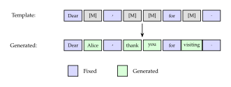
Diffusion models naturally support constrained generation: fixing certain tokens and generating the rest. For example:
Template filling: Given a template “Dear [NAME], Thank you for your [REASON]. We will [ACTION].” the diffusion model fills in the blanks using bidirectional context.
Lexically constrained generation: Requiring specific keywords to appear in the output can be enforced by initializing those tokens as unmasked.
Style transfer: Keeping content words fixed while regenerating function words can change the style of text while preserving meaning.
Biological Sequence Design
MDLM has been applied to DNA sequence modeling with competitive results. The masking-based approach is natural for biological sequences because:
Biological sequences are discrete (nucleotides or amino acids).
The function of a position depends on both flanking regions (bidirectional context).
Protein engineering often involves fixing certain regions (e.g., active sites) while optimizing others, naturally expressed as constrained diffusion.
Machine Translation and Editing
Non-autoregressive translation (NAT) is a long-standing goal in machine translation. Diffusion models provide a principled framework for NAT:
Encode the source sentence as context.
Initialize the target as fully masked: .
Run the reverse diffusion process conditioned on .
This allows the translation to be generated in parallel, with iterative refinement ensuring fluency and accuracy. The bidirectional context is particularly valuable for translation, where word order may differ between source and target languages.
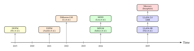
Historical Timeline and Development
The development of diffusion language models has been remarkably rapid. We present a timeline highlighting the key milestones:
Exercises
Exercise 1 (Forward Process Statistics).
Consider a sequence of length with the linear masking schedule .
What is the expected number of masked tokens at time ?
What is the variance of the number of masked tokens at time ?
What is the probability that at least 50 tokens are masked at ?
Hint: The number of masked tokens follows a Binomial distribution.
Exercise 2 (Reverse Posterior Verification).
Exercise 3 (Schedule Invariance).
Show that for the change of variables , the differential element transforms as: Verify this for the linear schedule and the exponential schedule .
Exercise 4 (Comparing AR and Diffusion Inference Cost).
Consider generating tokens with a dense Transformer of parameters, stored in bf16. Count both the weight traffic and the arithmetic, since the ratio between them is what decides where the machine runs.
An AR step with a KV cache reads all weights ( bytes) and does FLOPs for the one new token. What is the arithmetic intensity of a single step, and why does it not depend on ?
A diffusion step reads the same bytes but does FLOPs, since it evaluates positions in one pass. What is its arithmetic intensity?
Total FLOPs for the whole sequence: for AR over steps, and for diffusion over steps. Diffusion therefore does times more arithmetic. Using the H100 figures from Section Arithmetic Intensity Analysis (3.35,TB/s and 989.5,TFLOP/s dense
bf16, ridge at AI ), estimate the wall-clock time of each on the appropriate roof, and find the largest for which diffusion is still faster.Where does the argument break down as grows, once the attention term stops being negligible against ?
Exercise 5 (Implementing MDLM Loss).
Write pseudocode (or actual code in your language of choice) for the MDLM training loss. Your implementation should:
Sample a batch of sequences from the dataset.
Sample a random time for each sequence.
Mask tokens independently with probability .
Forward pass through a bidirectional Transformer.
Compute the -weighted cross-entropy loss over masked positions only.
Exercise 6 (SEDD Score Entropy).
Exercise 7 (Block Diffusion Trade-offs).
Consider a sequence of length generated using block diffusion with block size and denoising steps per block.
Express the total number of neural network forward passes as a function of and .
What is the total for with (fully autoregressive)? For with steps (a single diffused block)?
Treating as continuous, what block size minimizes the total forward passes if ? Which integer block sizes bracket that optimum?
Exercise 8 (Reversal Curse).
Explain mathematically why an autoregressive model trained with the factorization cannot guarantee that is well-modeled, even if is perfectly learned. Then explain why a masked diffusion model naturally avoids this issue.
Hint: Consider Bayes' theorem and what information the AR factorization provides about reverse conditionals.
Exercise 9 (Research: Designing a Better Remasking Strategy).
Propose a remasking strategy that goes beyond random and low-confidence remasking. Consider:
Using the model's uncertainty (e.g., entropy of the predicted distribution) rather than just the maximum probability.
Using positional information (e.g., remasking tokens that are far from already-confident tokens).
Using a learned remasking policy trained to minimize the expected number of denoising steps.
Discuss the trade-offs of each approach.
References
-
The reversal curse: LLMs trained on ``A is B'' fail to learn ``B is A''
BibTeX
@article{berglund2023reversal, title={The reversal curse: {LLMs} trained on ``{A} is {B}'' fail to learn ``{B} is {A}''}, author={Berglund, Lukas and Tong, Meg and Kaufmann, Max and Balesni, Mikita and Stickland, Asa Cooper and Korbak, Tomasz and Evans, Owain}, journal={arXiv preprint arXiv:2309.12288}, year={2023} }Journal article
-
Your absorbing discrete diffusion secretly models the conditional distributions of clean data
BibTeX
@article{shi2024absorbing, title={Your absorbing discrete diffusion secretly models the conditional distributions of clean data}, author={Ou, Jingyang and Nie, Shen and others}, journal={arXiv preprint arXiv:2406.03736}, year={2024} }Journal article
-
BERT: Pre-training of deep bidirectional transformers for language understanding
BibTeX
@article{devlin2019bert, title={{BERT}: Pre-training of deep bidirectional transformers for language understanding}, author={Devlin, Jacob and Chang, Ming-Wei and Lee, Kenton and Toutanova, Kristina}, journal={Proceedings of NAACL-HLT}, pages={4171--4186}, year={2019} }Journal article
-
MaskGIT: Masked generative image transformer
BibTeX
@article{chang2022maskgit, title={{MaskGIT}: Masked generative image transformer}, author={Chang, Huiwen and Zhang, Han and Jiang, Lu and Liu, Ce and Freeman, William T}, journal={Proceedings of the IEEE/CVF Conference on Computer Vision and Pattern Recognition}, pages={11315--11325}, year={2022} }Journal article
-
Large language diffusion models
BibTeX
@article{nie2025large, title={Large language diffusion models}, author={Nie, Shen and Zhu, Fengqi and You, Zebin and Zhang, Xiaolu and Ou, Jingyang and Hu, Jun and Zhou, Jun and Lin, Yankai and Wen, Ji-Rong and Li, Chongxuan}, journal={arXiv preprint arXiv:2502.09992}, year={2025} }Journal article
-
Block diffusion: Interpolating between autoregressive and diffusion language models
BibTeX
@article{arriola2024block, title={Block diffusion: Interpolating between autoregressive and diffusion language models}, author={Arriola, Marianne and Gokaslan, Aaron and Sahoo, Subham Sekhar and Kuleshov, Volodymyr}, journal={arXiv preprint arXiv:2503.09573}, note={ICLR 2025}, year={2025} }Journal article
-
Variational Diffusion Models
BibTeX
@inproceedings{kingma2021variational, title={Variational Diffusion Models}, author={Kingma, Diederik and Salimans, Tim and Poole, Ben and Ho, Jonathan}, booktitle={Advances in Neural Information Processing Systems}, volume={34}, pages={21696--21707}, year={2021} }Conference paper
-
Mercury: Ultra-fast language models based on diffusion
BibTeX
@article{khanna2025mercury, title={Mercury: Ultra-fast language models based on diffusion}, author={Khanna, Samar and Kharbanda, Siddhant and Li, Shufan and Varma, Harshit and Wang, Eric and Birnbaum, Sawyer and Luo, Ziyang and Miraoui, Yanis and Palrecha, Akash and Ermon, Stefano and Grover, Aditya and Kuleshov, Volodymyr}, journal={arXiv preprint arXiv:2506.17298}, year={2025} }Journal article
-
How discrete and continuous diffusion meet: Comprehensive analysis of discrete diffusion models via a stochastic integral framework
BibTeX
@article{chen2024discrete, title={How discrete and continuous diffusion meet: Comprehensive analysis of discrete diffusion models via a stochastic integral framework}, author={Ren, Yinuo and Chen, Haoxuan and others}, journal={arXiv preprint arXiv:2410.03601}, year={2024} }Journal article
-
Absorb and Converge: Provable Convergence Guarantee for Absorbing Discrete Diffusion Models
BibTeX
@article{liang2025absorb, title={Absorb and Converge: Provable Convergence Guarantee for Absorbing Discrete Diffusion Models}, author={Liang, Yuchen and Huang, Renxiang and Lai, Lifeng and Shroff, Ness and Liang, Yingbin}, journal={arXiv preprint arXiv:2506.02318}, year={2025} }Journal article
-
XLNet: Generalized autoregressive pretraining for language understanding
BibTeX
@article{yang2019xlnet, title={{XLNet}: Generalized autoregressive pretraining for language understanding}, author={Yang, Zhilin and Dai, Zihang and Yang, Yiming and Carbonell, Jaime and Salakhutdinov, Ruslan R and Le, Quoc V}, journal={Advances in Neural Information Processing Systems}, volume={32}, year={2019} }Journal article
-
Language Models are Unsupervised Multitask Learners
BibTeX
@techreport{radford2019language, title={Language Models are Unsupervised Multitask Learners}, author={Radford, Alec and Wu, Jeff and Child, Rewon and Luan, David and Amodei, Dario and Sutskever, Ilya}, institution={OpenAI}, year={2019} }Technical report
-
LLaMA: Open and Efficient Foundation Language Models
BibTeX
@article{touvron2023llama, author = {Touvron, Hugo and Lavril, Thibaut and Izacard, Gautier and Martinet, Xavier and Lachaux, Marie-Anne and others}, title = {{LLaMA}: Open and Efficient Foundation Language Models}, journal = {arXiv preprint arXiv:2302.13971}, year = {2023} }Journal article
-
Denoising Diffusion Probabilistic Models
BibTeX
@inproceedings{ho2020denoising, title={Denoising Diffusion Probabilistic Models}, author={Ho, Jonathan and Jain, Ajay and Abbeel, Pieter}, booktitle={Advances in Neural Information Processing Systems}, volume={33}, pages={6840--6851}, year={2020} }Conference paper
-
High-resolution image synthesis with latent diffusion models
BibTeX
@article{rombach2022high, title={High-resolution image synthesis with latent diffusion models}, author={Rombach, Robin and Blattmann, Andreas and Lorenz, Dominik and Esser, Patrick and Ommer, Bj{\"o}rn}, journal={Proceedings of the IEEE/CVF Conference on Computer Vision and Pattern Recognition}, pages={10684--10695}, year={2022} }Journal article
-
Hierarchical text-conditional image generation with CLIP latents
BibTeX
@article{ramesh2022hierarchical, title={Hierarchical text-conditional image generation with {CLIP} latents}, author={Ramesh, Aditya and Dhariwal, Prafulla and Nichol, Alex and Chu, Casey and Chen, Mark}, journal={arXiv preprint arXiv:2204.06125}, year={2022} }Journal article
-
Structured denoising diffusion models in discrete state-spaces
BibTeX
@article{austin2021structured, title={Structured denoising diffusion models in discrete state-spaces}, author={Austin, Jacob and Johnson, Daniel D and Ho, Jonathan and Tarlow, Daniel and van den Berg, Rianne}, journal={Advances in Neural Information Processing Systems}, volume={34}, pages={17981--17993}, year={2021} }Journal article
-
Simple and effective masked diffusion language models
BibTeX
@article{sahoo2024simple, title={Simple and effective masked diffusion language models}, author={Sahoo, Subham Sekhar and Arriola, Marianne and Schiff, Yair and Gokaslan, Aaron and Marroquin, Edgar and Chiu, Justin T and Rush, Alexander and Kuleshov, Volodymyr}, journal={Advances in Neural Information Processing Systems}, volume={37}, year={2024} }Journal article
-
Discrete diffusion modeling by estimating the ratios of the data distribution
BibTeX
@article{lou2024discrete, title={Discrete diffusion modeling by estimating the ratios of the data distribution}, author={Lou, Aaron and Meng, Chenlin and Ermon, Stefano}, journal={Proceedings of the International Conference on Machine Learning}, year={2024} }Journal article
-
LLaDA 2.0: Scaling up diffusion language models to 100B
BibTeX
@article{llada2, title={{LLaDA} 2.0: Scaling up diffusion language models to 100B}, author={Bie, Tiwei and Cao, Maosong and Chen, Kun and Du, Lun and others}, journal={arXiv preprint arXiv:2512.15745}, year={2025} }Journal article
-
The Neural Autoregressive Distribution Estimator
BibTeX
@inproceedings{larochelle2011neural, title={The Neural Autoregressive Distribution Estimator}, author={Larochelle, Hugo and Murray, Iain}, booktitle={Proceedings of the 14th International Conference on Artificial Intelligence and Statistics (AISTATS)}, year={2011} }Conference paper
-
MADE: Masked Autoencoder for Distribution Estimation
BibTeX
@inproceedings{germain2015made, title={{MADE}: Masked Autoencoder for Distribution Estimation}, author={Germain, Mathieu and Gregor, Karol and Murray, Iain and Larochelle, Hugo}, booktitle={Proceedings of the 32nd International Conference on Machine Learning (ICML)}, year={2015} }Conference paper
-
Pixel Recurrent Neural Networks
BibTeX
@inproceedings{oord2016pixel, title={Pixel Recurrent Neural Networks}, author={van den Oord, A\"{a}ron and Kalchbrenner, Nal and Kavukcuoglu, Koray}, booktitle={Proceedings of the 33rd International Conference on Machine Learning (ICML)}, year={2016} }Conference paper
-
Conditional Image Generation with PixelCNN Decoders
BibTeX
@inproceedings{oord2016conditional, title={Conditional Image Generation with {PixelCNN} Decoders}, author={van den Oord, A\"{a}ron and Kalchbrenner, Nal and Espeholt, Lasse and Kavukcuoglu, Koray and Vinyals, Oriol and Graves, Alex}, booktitle={Advances in Neural Information Processing Systems (NeurIPS)}, year={2016} }Conference paper
-
Diffusion-LM improves controllable text generation
BibTeX
@article{li2022diffusion, title={Diffusion-{LM} improves controllable text generation}, author={Li, Xiang Lisa and Thickstun, John and Gulrajani, Ishaan and Liang, Percy and Hashimoto, Tatsunori B}, journal={Advances in Neural Information Processing Systems}, volume={35}, pages={4328--4343}, year={2022} }Journal article
-
Diffuseq: Sequence to sequence text generation with diffusion models
BibTeX
@article{gong2023diffuseq, title={Diffuseq: Sequence to sequence text generation with diffusion models}, author={Gong, Shansan and Li, Mukai and Feng, Jiangtao and Wu, Zhiyong and Kong, Lingpeng}, journal={Proceedings of the International Conference on Learning Representations}, year={2023} }Journal article
-
A continuous time framework for discrete denoising models
BibTeX
@article{campbell2022continuous, title={A continuous time framework for discrete denoising models}, author={Campbell, Andrew and Benton, Joe and De Bortoli, Valentin and Rainforth, Tom and Deligiannidis, George and Doucet, Arnaud}, journal={Advances in Neural Information Processing Systems}, volume={35}, year={2022} }Journal article
-
Improved Denoising Diffusion Probabilistic Models
BibTeX
@inproceedings{nichol2021improved, title={Improved Denoising Diffusion Probabilistic Models}, author={Nichol, Alexander Quinn and Dhariwal, Prafulla}, booktitle={International Conference on Machine Learning}, pages={8162--8171}, year={2021}, organization={PMLR} }Conference paper
-
Classifier-free diffusion guidance
BibTeX
@article{ho2022classifier, title={Classifier-free diffusion guidance}, author={Ho, Jonathan and Salimans, Tim}, journal={arXiv preprint arXiv:2207.12598}, year={2022} }Journal article