21 Audio and Music Generation
Why Audio Generation?
Consider a ten-second clip of a jazz trio: a piano outlines a chord progression, a bass walks through the changes, and brushes dance on a snare drum. The corresponding digital waveform contains roughly 441,000 samples (at 44.1,kHz), each carrying amplitude information at 16-bit resolution. To a generative model, this clip is a point in , and the space of perceptually valid jazz trio recordings occupies a vanishingly thin manifold within that vast ambient space. The challenge of audio generation is to learn the structure of this manifold well enough to draw new points from it on demand.
Why should we care? The practical applications are abundant. Text-to-speech systems convert written language to natural sounding utterances, powering virtual assistants and accessibility tools. Text-to-music models compose novel audio given natural-language prompts such as “a melancholic cello solo over soft rain.” Sound effect generation synthesises Foley audio for film and game production. Audio inpainting fills gaps in corrupted recordings, and voice conversion transforms the timbre of a speaker while preserving linguistic content. These tasks share a common mathematical substrate: learning a conditional or unconditional distribution over waveforms and sampling from it efficiently.
Key Idea.
Despite their surface diversity, all audio generation tasks reduce to the same abstract problem: model a distribution (or for conditional generation) over sequences , where is the number of audio samples, and generate new sequences by sampling from the learned distribution. The differences between tasks lie in the conditioning signal (text, melody, video, speaker embedding) and in which aspects of the output the user cares about (intelligibility, musicality, timbral fidelity).
The Dimensionality of Sound
The raw dimensionality of audio signals dwarfs that of the images we encountered in earlier chapters, yet remains below the extreme scales of video. tab:audiogen:dimensionality makes this concrete.
tableDimensionality of audio signals at various
durations and sample rates. CD-quality audio uses 44.1,kHz;
speech models commonly use 16,kHz.
Signal Sample Rate Duration Dimensions Speech utterance 16,kHz 3,s Speech paragraph 16,kHz 30,s Music clip 44.1,kHz 10,s Full song 44.1,kHz 4,min Stereo full song 44.1,kHz 4,min RGB image – –
A single second of CD-quality mono audio contains 44,100 floating-point values. A three-minute pop song therefore lives in a space of dimension ; in stereo, this doubles to . It is duration, not instantaneous richness, that does the damage: a ten-second music clip () is actually a little smaller than a single RGB image (), but the three-minute song is a full order of magnitude larger, and its stereo version twenty times larger. An image generator is asked for one such object; a music generator is asked for a signal that keeps being coherent for minutes.
Remark 1.
The high dimensionality of raw waveforms motivates the development of compressed representations: mel-spectrograms reduce the time axis by hop-size factors of 256–512 and the frequency axis to 80–128 mel bins, while neural audio codecs compress a full second of audio into as few as 50–75 discrete tokens. Nearly every modern audio generation system operates in one of these compressed spaces rather than directly on the waveform. Sections Audio Signal Processing Foundations and Neural Audio Codecs develop these representations in detail.
Remark 2.
Audio and image generation share many mathematical foundations (GANs, VAEs, diffusion models, flow matching), but two structural differences profoundly affect model design. First, audio is inherently sequential: the natural causal ordering of time provides a strong inductive bias for autoregressive models, which have no equally natural ordering for 2D images. Second, the perceptual metric for audio is fundamentally different from that for images. Human auditory perception is exquisitely tuned to spectral envelope, pitch, and temporal dynamics, and comparatively tolerant of the relative phase of a steady tone's partials (a tolerance that is easy to overstate; see insight:audiogen:phase-problem), while visual perception is dominated by spatial frequency and colour statistics. These perceptual differences motivate the specialised loss functions (mel-spectrogram loss, multi-resolution STFT loss) and representations (mel-spectrograms, codec tokens) that this chapter develops.
A Brief History of Audio Generation
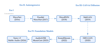
The history of neural audio generation can be divided into four overlapping eras, each defined by the dominant generative paradigm. We summarise them here to provide context for the technical sections that follow; the reader should consult the original papers for full details.
Era I: Concatenative and parametric synthesis (pre-2016).
Classical text-to-speech systems either concatenated recorded speech segments from large databases or drove parametric vocoders with hand-engineered acoustic features. The quality ceiling was unmistakable: concatenative systems sounded choppy at segment boundaries, and parametric vocoders produced a characteristic “buzzy” timbre that listeners found unnatural.
Era II: Autoregressive waveform models (2016–2019).
DeepMind's WaveNet [13] demonstrated that an autoregressive model predicting one sample at a time could produce strikingly natural speech. The model factorised the joint distribution as (Wavenet Factor) with each conditional implemented by a dilated causal convolution stack. The catch was speed: generating one second of 16,kHz audio required 16,000 sequential forward passes. Parallel WaveNet [14] and WaveRNN [15] addressed inference cost, but the autoregressive bottleneck remained a theme.
Era III: GAN and diffusion vocoders (2019–2022).
GAN-based vocoders such as MelGAN [16], HiFi-GAN [17], and UnivNet [18] replaced autoregressive generation with feed-forward synthesis, achieving real-time waveform generation on a single GPU\@. Concurrently, diffusion-based vocoders (DiffWave [19], WaveGrad [20]) applied the denoising diffusion framework of 19 to the audio domain. These models serve as the “decoder” in many two-stage generation pipelines.
Era IV: Foundation models for audio (2023–present).
The convergence of large language models, neural audio codecs, and latent diffusion has produced a new generation of systems capable of generating high-fidelity, long-form audio from text prompts. AudioLDM [21] applies latent diffusion to mel-spectrograms. MusicGen [22] generates music autoregressively over the discrete tokens of an EnCodec codec. Stable Audio [23] operates a latent diffusion transformer in the continuous latent space of a variational autoencoder. Commercial systems such as Suno and Udio generate full songs with vocals, approaching (and sometimes passing) human-level quality in listener studies.
Historical Note.
The pace of progress. WaveNet appeared in September 2016; barely seven years later, Suno v3 could generate a full two-minute pop song with lyrics, melody, harmony, and studio-quality mixing from a single text prompt. This trajectory, from sample-level autoregression to codec-based language modelling and latent diffusion, mirrors the image generation revolution but unfolds in a domain with fundamentally different signal characteristics. Figure 1 sketches the key milestones.
Chapter Roadmap
This chapter develops the mathematical and architectural foundations of modern audio generation systems. The narrative is organised into a progression from signal-level building blocks to complete generation pipelines.
Audio signal processing (Audio Signal Processing Foundations). We formalise the Short-Time Fourier Transform, the mel scale, and the mel-spectrogram, establishing the standard input representations used throughout the chapter.
Neural audio vocoders (Neural Audio Vocoders). We study HiFi-GAN and related architectures that convert mel-spectrograms back into high-fidelity waveforms, connecting their discriminator designs to the GAN theory of 9.
Neural audio codecs (Neural Audio Codecs). We develop Residual Vector Quantisation and its application in SoundStream, EnCodec, and DAC, which compress audio into sequences of discrete tokens amenable to language-model-style generation.
CLAP and contrastive audio–text alignment (CLAP: Contrastive Language–Audio Pretraining). We formalise the contrastive loss that learns a joint embedding space for audio and text, enabling text-conditioned generation.
Autoregressive generation over codec tokens (later sections). We study MusicLM and MusicGen, which treat audio generation as a sequence modelling problem over discrete codec codes.
Latent diffusion and flow matching for audio (later sections). We develop AudioLDM, Stable Audio, and related systems that apply continuous generative models in compressed latent spaces.
Evaluation, ethics, and open problems (later sections). We discuss Fréchet Audio Distance, perceptual metrics, watermarking, and the societal implications of generative audio.
Throughout, we assume familiarity with the fundamentals of generative adversarial networks (9), variational autoencoders (15), diffusion models (19), and normalising flows (18). Readers seeking background on these topics should consult the corresponding chapters before proceeding.
Audio Signal Processing Foundations
Before we can generate audio, we must understand how audio is represented, transformed, and compressed. This section develops the mathematical machinery that every subsequent section relies upon: the Short-Time Fourier Transform (STFT), the mel frequency scale, and the mel-spectrogram. These are not mere engineering details; they encode deep facts about human perception and signal structure that profoundly shape the design of generative models.
Digital Audio Signals
A continuous-time audio signal is a real-valued function of time, . Digital audio is obtained by sampling at a fixed rate (the sampling rate or sample rate), producing a discrete sequence (Sampling) where is the total number of samples and is the signal duration in seconds. We collect these samples into a vector .
Definition 1 (Digital Audio Signal).
A digital audio signal is a vector whose -th entry represents the amplitude of a continuous-time acoustic waveform sampled at rate hertz. The Nyquist frequency is the highest frequency that can be faithfully represented without aliasing.
Standard sample rates include 8,kHz (telephony), 16,kHz (speech processing), 22.05,kHz (compressed music), 44.1,kHz (CD-quality), and 48,kHz (professional audio and video). The choice of determines both the bandwidth and the dimensionality of the generative modelling problem.
Remark 3.
In practice, each sample is stored as a fixed-point integer (e.g., 16-bit PCM, giving quantisation levels) or a 32-bit floating-point number. For the purposes of generative modelling, we treat as a real-valued vector and defer quantisation to the final output stage. This is analogous to working with continuous pixel intensities in image generation rather than discrete 8-bit values.
Example 1 (Speech vs. music sample rates).
A text-to-speech system operating at ,Hz represents frequencies up to 8,kHz, which suffices for intelligible speech but discards much of the spectral richness that makes natural voices warm and distinctive. A music generation system typically requires ,Hz or higher to capture the full range of human hearing (approximately 20,Hz to 20,kHz), the shimmer of cymbals, the breathiness of a flute, the harmonic overtones of a bowed string. This nearly threefold increase in sample rate translates directly into higher-dimensional generation problems.
Proposition 1 (Shannon–Nyquist Sampling Theorem).
Let be a band-limited continuous signal whose Fourier transform satisfies for . Then can be perfectly reconstructed from its samples if and only if . If , the sampled signal suffers from aliasing: high-frequency components fold back into the representable bandwidth, creating artefacts that cannot be removed by post-processing.
Proof.
The sampled signal's spectrum is the periodisation . When , the copies do not overlap, so can be recovered by applying an ideal low-pass filter with cutoff . When , adjacent copies overlap (aliasing), and the original spectrum cannot be recovered.
Caution.
Aliasing is not only a concern during recording; it can also arise during generation. If a neural vocoder or codec decoder produces frequency content above the Nyquist frequency (e.g., due to nonlinear activations in transposed convolution layers), this energy aliases back into the audible band, producing metallic or buzzy artefacts. Anti-aliased activation functions, as used in BigVGAN [1], mitigate this problem by low-pass filtering the hidden representations after each nonlinearity.
The Short-Time Fourier Transform
The Fourier transform reveals the frequency content of a signal, but it provides no information about when those frequencies occur. For audio generation, temporal localisation is essential: a piano note that begins at time ,s and ends at ,s must be placed correctly in the output waveform. The Short-Time Fourier Transform (STFT) resolves this tension by applying the Fourier transform to short, overlapping windows of the signal.
Definition 2 (Short-Time Fourier Transform).
Let be a digital audio signal and let be a window function of length . The Short-Time Fourier Transform of is the complex-valued matrix with entries (STFT) where is the frequency bin index with , is the frame index with , is the hop size (the number of samples between successive frames), and .
Each column of is the discrete Fourier transform (DFT) of a windowed segment of . The window function (commonly Hann, Hamming, or Blackman) tapers the segment smoothly to zero at its edges, suppressing spectral leakage from discontinuities at the segment boundaries.
Remark 4.
Typical parameter choices in audio generation are or , hop size or , and a Hann window. With ,Hz, , and , each frame spans approximately 46,ms and frames overlap by 75%. The resulting STFT has frequency bins and time frames.
The STFT is invertible (under mild conditions on the window), which is crucial: a vocoder must be able to reconstruct a waveform from a modified spectrogram. The inverse STFT (iSTFT) recovers the signal by applying the inverse DFT to each frame, multiplying by a synthesis window, and overlap-adding the results.
Definition 3 (Inverse STFT via Overlap-Add).
Given the STFT matrix and a synthesis window , the inverse STFT is (Istft) where is the inverse DFT of the -th frame of , and the denominator normalises for the overlapping windows.
For the inverse to be exact, the analysis and synthesis windows must satisfy a completeness condition.
Proposition 2 (Constant Overlap-Add (COLA) Condition).
Let be the analysis window and the synthesis window, both of length . Perfect reconstruction holds, i.e., for all , if and only if (COLA) for some constant . When (the common case), this reduces to (COLA Symmetric)
Proof.
Substituting into (Istft) and using the definition of from (STFT), the numerator becomes The sum over produces a Kronecker delta , collapsing the inner sum to . Thus the numerator equals , and dividing by the denominator yields whenever this sum is nonzero and constant.
Example 2 (COLA verification for the Hann window).
The Hann window of length is for . With hop size (50% overlap), the unsquared window is COLA: the two overlapping copies at and contribute , with , so for all . This is the familiar fact that a Hann analysis window with a rectangular synthesis window reconstructs exactly at 50% overlap.
The squared window, which is what (COLA Symmetric) requires when , does not share this property. The same two copies give (COLA HANN HALF) which sweeps the whole interval as runs over one hop. Its mean is , and is the mean of over the window - which is exactly the tempting miscalculation to avoid, because COLA is a statement about every , not about an average. Plain overlap-add with at 50% overlap therefore amplitude-modulates the reconstruction by , once per hop.
With (75% overlap), by contrast, the four overlapping copies of do sum to the constant for every . Only in this case is the denominator in (Istft) constant, and this - not 50% - is why 75% overlap with a Hann window is the default in vocoder and codec training pipelines.
The STFT decomposes the signal into three informative representations, each useful in different generative contexts.
Definition 4 (STFT Magnitude, Phase, and Power Spectrogram).
Given the STFT :
The magnitude spectrogram is with entries .
The phase spectrogram is with entries .
The power spectrogram is with entries .
Insight.
Most audio generation models predict only the magnitude (or log-magnitude) spectrogram and discard phase information. This is usually justified by the claim that human auditory perception is sensitive to spectral magnitude and not to phase. That claim is an overstatement of a much narrower fact. What listeners are largely insensitive to is the relative phase of the partials of a single steady tone (Ohm's law of acoustics); phase still carries transient timing, the attack signature that separates a struck note from a bowed one, and - in stereo - the interaural cues that place a source in space. Nor does insensitivity license discarding phase, because an arbitrary magnitude array paired with an arbitrary phase array is generally inconsistent: no waveform has that STFT at all. Most of the audible damage done by magnitude-only models comes from this inconsistency, not from phase being inaudible.
Reconstructing a waveform from magnitude alone therefore requires estimating a phase field that is at least self-consistent; the classical Griffin-Lim algorithm [2] iteratively projects between the STFT domain and the time domain to find such a phase (a consistent one, not necessarily the true one), while neural vocoders (see Neural Audio Vocoders) learn to synthesise phase implicitly as part of the waveform generation process.
Proposition 3 (STFT as a Linear Operator).
The STFT defines a linear map . That is, for any and : (STFT Linear) This linearity has an important practical consequence: if a model generates two spectrogram components separately (e.g., a harmonic component and a noise component), their sum in the STFT domain corresponds to the STFT of the sum of the corresponding time-domain signals.
Proof.
From (STFT), each entry is a weighted sum of the signal samples: . Substituting and using linearity of the finite sum yields the result.
Proposition 4 (Parseval's Theorem for the STFT).
If the analysis window satisfies the COLA condition (Proposition 2) with constant , then the signal energy is preserved (up to normalisation) in the STFT domain: (STFT Parseval) This energy preservation property ensures that the STFT does not artificially amplify or attenuate any portion of the signal, which is critical when using STFT-domain losses for training generative models.
Proof.
By Parseval's theorem for the DFT, the energy in the -th windowed frame satisfies . Summing over all frames and using the COLA condition yields the stated identity.
Example 3 (STFT compression ratio).
A 10-second audio clip at ,Hz has real-valued samples. The STFT with and produces frequency bins and frames. The magnitude spectrogram has entries, roughly the size of the original signal. However, the log-mel-spectrogram with has only entries, a compression factor of . This modest spatial compression, combined with the perceptual relevance of mel features, is why the mel-spectrogram has become the standard intermediate representation.
Remark 5.
The STFT is subject to the Heisenberg–Gabor uncertainty principle: the product of time resolution and frequency resolution cannot be made arbitrarily small. Specifically, for a Gaussian window (which minimises the uncertainty product), (Gabor Limit) A large FFT window gives fine frequency resolution at the cost of poor temporal localisation; a small window gives fine temporal resolution at the cost of smeared frequencies. This fundamental tradeoff explains why the multi-resolution STFT loss (Definition 12) uses multiple window sizes: no single window can simultaneously capture both the transient attack of a snare drum and the precise pitch of a sustained violin note.
The Mel Scale and Mel-Spectrogram
The linear frequency axis of the STFT does not match human auditory perception. We perceive pitch differences on a roughly logarithmic scale: the perceptual distance between 100,Hz and 200,Hz (one octave) is much greater than that between 5,000,Hz and 5,100,Hz, even though the absolute difference in hertz is the same. The mel scale provides a frequency warping that better reflects this perceptual nonlinearity.
Definition 5 (Mel Scale).
The mel scale is a perceptual frequency scale defined by the mapping , (MEL Scale) where is the frequency in hertz. The inverse mapping is (MEL Inverse) The mel scale is approximately linear below 1,kHz and approximately logarithmic above 1,kHz, matching the frequency resolution of the human cochlea.
Remark 6.
The mel scale was proposed by Stevens, Volkmann, and Newman in 1937, based on experiments asking listeners to adjust a tone until it sounded “half as high” as a reference. The name “mel” derives from “melody,” reflecting the scale's connection to perceived pitch. Several competing formulas exist (e.g., the HTK variant uses ), but the logarithmic formula in (MEL Scale) is the most widely used in modern audio generation systems.
Proposition 5 (Mel Scale Asymptotics).
The mel scale exhibits two distinct regimes:
Low frequencies (,Hz): using for small , (MEL LOW FREQ) The mel scale is approximately linear, with 1,mel 0.62,Hz.
High frequencies (,Hz): using , (MEL HIGH FREQ) The mel scale is approximately logarithmic.
Proof.
Both results follow from standard asymptotic expansions of . For part 1, the first-order Taylor expansion applies when . For part 2, when , the additive 1 in the argument becomes negligible, yielding .
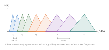
To construct a mel-spectrogram, we apply a bank of triangular filters, spaced uniformly on the mel scale, to the power (or magnitude) spectrogram.
Definition 6 (Mel Filterbank).
Let be the desired number of mel bands. Choose centre frequencies that are equally spaced on the mel scale between and , where and define the frequency range of interest. The -th triangular filter () is (MEL Filter) where is the frequency corresponding to DFT bin . The filters are assembled into the mel filterbank matrix , with .
Definition 7 (Mel-Spectrogram).
Given the magnitude spectrogram and the mel filterbank matrix , the mel-spectrogram is (MEL Spectrogram) or, in log scale, (LOG MEL) where is a small constant (typically or ) for numerical stability. The log-mel-spectrogram is the most common input representation for neural audio generation models.
Figure 2 illustrates the mel filterbank and the pipeline from waveform to mel-spectrogram.

Proposition 6 (Mel Filterbank as Information Bottleneck).
The mel filterbank matrix with has rank at most . The mapping is therefore a lossy projection: the null space has dimension at least , and any spectral variation lying in is irretrievably lost. With and , the filterbank discards at least dimensions of spectral information per frame.
Proof.
Since with , . By the rank-nullity theorem, . Any vector in is mapped to zero, so spectral detail in those directions cannot be recovered from the mel-spectrogram.
Representation Taxonomy
Modern audio generation systems operate on one of several representations, each offering a different trade-off between reconstruction fidelity, dimensionality, and suitability for generative modelling. We classify the main options here for reference; subsequent sections develop each in detail.
Raw waveform (). The highest-fidelity representation, but extremely high-dimensional and temporally fine-grained. Direct waveform models (WaveNet, SampleRNN) operate here but face severe computational costs.
Mel-spectrogram (). A compressed, perceptually motivated 2D representation. Since , the number of stored values falls by a factor of relative to the waveform (for and , a factor of 4), but reconstruction requires a vocoder to estimate phase and fine spectral detail.
Discrete codec tokens (). A sequence of integer codes produced by a neural audio codec (SoundStream, EnCodec, DAC) with quantisation levels and time frames. This is the most compressed representation, enabling language-model-style generation, but introduces quantisation artefacts.
Continuous latents (). The bottleneck representation of a continuous (non-quantised) autoencoder. Latent diffusion and flow matching models operate here, combining the compression benefits of codecs with the smoothness of continuous spaces.
tableAudio representation taxonomy. Each representation
trades off dimensionality, information content, and compatibility
with different generative model families. The reduction factors
are those of the worked configuration in
Example 4 (10,s at 24,kHz, hop and
stride 320, , latent width , ); they
are configuration-dependent, and the rows are ordered by the factor
they achieve, not by fidelity.
Representation Type Dim. reduction Invertible? Compatible models Raw waveform Yes AR, GAN Continuous latent No (decoder) Diffusion, flow Mel-spectrogram No (vocoder) Diffusion, flow Discrete tokens No (decoder) AR, masked LM
The ordering deserves comment, because it is not the one a reader might expect. A continuous codec latent is less compressed than a mel-spectrogram in this configuration - 96,000 numbers against 60,000 - and yet it is the better representation to generate in. Compression and modelling difficulty are two different axes, and the rest of this chapter is largely the story of how they came apart.
Remark 7 (Ordering the ladder by reconstruction ceiling).
It is tempting to write down a single chain in the entropies and declare a strict hierarchy. Resist it. Two of the four quantities are differential entropies of continuous variables and one is the discrete entropy of a finite alphabet, so they are not on a common scale and their signs are not even convention-free. Worse, the middle inequality is simply not true of the systems in this chapter: the codec latent is not computed from , it is computed from the waveform, and it is trained end to end for waveform reconstruction. In the configuration of Example 4 it holds more numbers than the mel-spectrogram does and it retains the phase information that the mel-spectrogram destroys outright. The two are not comparable by inclusion at all.
What survives, and is what we actually use, is an ordering by reconstruction ceiling - the best fidelity any decoder could achieve from that representation:
discards phase and all spectral detail inside a mel band, and is irreversible in the strong sense of Proposition 6: the filterbank has a null space of dimension at least .
discards whatever the autoencoder bottleneck of width cannot carry, but nothing by construction; a wider or better-trained autoencoder raises the ceiling continuously.
adds a quantisation error of per frame on top of that (Theorem 1), and is the only step whose loss can be driven towards zero simply by spending more bits.
The generative modelling task typically becomes easier as one moves down this list, because the representation gets shorter, smoother, or discrete. But easier-to-model and lower-fidelity are separate properties, and the mel-spectrogram is the cautionary case: it is both smaller than the codec latent and the one with the lower ceiling, which is precisely why the field moved off it.
Caution.
The choice of representation is not merely an implementation detail; it fundamentally determines which generative model families are applicable. Autoregressive language models require discrete tokens (representation 3). Diffusion and flow matching require continuous spaces (representations 2 or 4). GANs can operate on either waveforms (1) or spectrograms (2). Choosing a representation is therefore inseparable from choosing a generative paradigm.
Example 4 (Representation dimensions for 10,s of audio at 24,kHz).
| Representation | Shape | Dims | Type |
| Raw waveform | 240,000 | ||
| Mel-spectrogram (, ) | 60,000 | ||
| Continuous latent (, ) | 96,000 | ||
| Codec tokens (, ) | 6,000 |
Neural Audio Vocoders
A vocoder is a system that converts a compact acoustic representation (classically, linear predictive coding parameters; in modern systems, a mel-spectrogram or similar feature) into a waveform. In the context of audio generation, the vocoder is the final stage that transforms a generated spectrogram into an audible signal. Its quality sets the ceiling for the overall system: a perfect generative model paired with a poor vocoder will produce poor audio.
Neural vocoders have evolved rapidly since WaveNet first demonstrated that a neural network could synthesise perceptually natural waveforms. In this section, we focus on HiFi-GAN [17], which has become the de facto standard vocoder in modern audio generation pipelines due to its combination of high fidelity, fast inference, and training stability. We develop its architecture in detail, connecting its multi-scale and multi-period discriminator designs to the GAN theory developed in 9.
The Vocoding Problem
Formally, the vocoding problem is a conditional generation task.
Definition 8 (Vocoding).
Given a mel-spectrogram , the vocoding problem is to generate a waveform such that:
sounds perceptually indistinguishable from the ground-truth waveform that produced , and
the mel-spectrogram of closely matches .
Since the mel-spectrogram discards phase and fine spectral detail, the mapping is inherently one-to-many: many waveforms share the same mel-spectrogram. The vocoder must learn to sample from the conditional distribution .
Remark 8.
The vocoder performs a massive upsampling. A mel-spectrogram at bands with hop size has values, while the corresponding waveform has samples. The upsampling factor along the time axis is , and the vocoder must fill in all the fine temporal structure (individual oscillation cycles, transient attacks, noise textures) that the mel-spectrogram averages over.
Historical Note.
The evolution of neural vocoders. The vocoder landscape has evolved through three generations. First-generation models (WaveNet, 2016; WaveRNN, 2018) achieved high quality through autoregressive sample-by-sample generation, but required seconds to minutes of computation per second of audio. Second-generation models (Parallel WaveNet, 2018; WaveGlow, 2019) used knowledge distillation or flow-based architectures to achieve parallel synthesis, reducing latency to real-time but at the cost of increased model complexity and training difficulty. Third-generation models (MelGAN, 2019; HiFi-GAN, 2020; BigVGAN, 2023) adopted GAN training with carefully designed discriminators, achieving both high quality and extreme speed (100–300 real-time on GPU). HiFi-GAN's insight that periodic and multi-scale discriminators complement each other has proven remarkably durable: variants of its discriminator architecture appear in nearly every subsequent vocoder and neural audio codec.
tableComparison of neural vocoder approaches. Speed is
measured relative to real-time on a single GPU\@. MOS denotes
mean opinion score on a 1–5 scale.
Model Paradigm Speed MOS Key Innovation WaveNet Autoregressive 0.001 4.2 Dilated causal conv. WaveRNN Autoregressive 0.4 4.1 Subscale prediction WaveGlow Flow 10 4.0 Invertible 11 conv. MelGAN GAN 100 3.8 Multi-scale disc. HiFi-GAN GAN 170 4.3 MPD + MSD BigVGAN GAN 120 4.4 Anti-aliased + Snake
HiFi-GAN: Generator Architecture
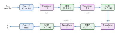
The HiFi-GAN generator is a fully convolutional feed-forward network that progressively upsamples the mel-spectrogram to the waveform sampling rate through a cascade of transposed convolution blocks, each followed by a multi-receptive-field fusion (MRF) module.
Definition 9 (HiFi-GAN Generator).
The HiFi-GAN generator consists of:
An input convolution that projects the -dimensional mel features to a high-dimensional channel space of width (typically 512).
A sequence of upsampling blocks, where the -th block applies a transposed 1D convolution with stride , increasing the temporal resolution by a factor of . The strides are chosen so that , the hop size used during mel-spectrogram extraction.
Within each upsampling block, a multi-receptive-field fusion (MRF) module consisting of parallel residual blocks, each with a different kernel size and dilation pattern. The outputs of the branches are summed (or averaged) to produce the block output: (MRF) where denotes the upsampled hidden representation from the transposed convolution.
A final convolution with a activation that maps the -channel hidden state to a single-channel waveform .
Example 5 (Typical HiFi-GAN configuration).
The “V1” configuration of HiFi-GAN uses , upsampling blocks with strides (so that ), and residual blocks per MRF module with kernel sizes . The total parameter count is approximately 14 million, and inference runs at over 100 real-time on a single GPU\@. Lighter configurations (“V2”, “V3”) trade quality for speed by reducing and the number of residual blocks.
Remark 9.
The MRF module is central to HiFi-GAN's success. By fusing the outputs of residual blocks with kernel sizes and dilation rates (or for the smallest kernel), each MRF module simultaneously captures patterns at multiple temporal scales within a single upsampling stage. Small kernels capture fine-grained sample-level correlations (e.g., the waveform of a single pitch cycle), while large kernels capture broader patterns (e.g., the modulation envelope of a tremolo effect). This multi-scale design within the generator complements the multi-scale structure of the discriminators.
Multi-Period and Multi-Scale Discriminators
The adversarial training of HiFi-GAN relies on two complementary discriminator families, each designed to capture different structural properties of audio waveforms. The design of these discriminators reflects a deep understanding of audio signal structure and connects directly to the GAN theory developed in 9 and the Wasserstein framework of 10.
Definition 10 (Multi-Period Discriminator (MPD)).
The multi-period discriminator consists of sub-discriminators , where is a set of prime periods. Each sub-discriminator operates as follows:
Reshape the 1D waveform into a 2D tensor of shape by folding every -th sample into a column.
Apply a stack of 2D strided convolutions to this reshaped signal, producing a scalar prediction .
Each sub-discriminator “sees” the waveform at a different periodic granularity: captures even/odd sample structure, detects triplet patterns, and so on. The prime periods ensure that no two sub-discriminators share the same periodic folding.
Insight.
Audio waveforms are highly periodic: a sung vowel at 220,Hz repeats its fundamental cycle every samples (at ,Hz). The MPD exploits this structure by reshaping the waveform so that periodic patterns become spatial patterns in a 2D grid, which standard 2D convolutions can detect efficiently. Using prime periods guarantees that the sub-discriminators provide non-redundant feedback about different periodic components of the signal.
Proposition 7 (MPD Period Coverage).
Let be the set of MPD periods and write . Among the integer periods , exactly are divisible by at least one , so that the corresponding sub-discriminator sees a perfectly aligned periodic pattern. The remaining periods (20.8%) are divisible by none of them. The coverage fraction is over every window of consecutive integers, so the bound is not a threshold beyond which coverage degrades; it is simply the period of the pattern.
Proof.
By the Chinese remainder theorem the residue of modulo determines divisibility by each , so the covered and uncovered sets are both unions of residue classes mod and the fraction is the same in every window of length . Inclusion and exclusion over the five primes gives an uncovered count of , leaving covered.
Caution.
Two things this proposition does not say are worth stating plainly, because both are easy to assume.
First, it is not true that “every composite period has a prime factor in ”. The uncovered periods are exactly those coprime to , and they include composites as well as primes: and are both invisible to every sub-discriminator, as are , , and themselves. Adding to would recover but would leave ; no finite prime set covers every integer.
Second, and more importantly in practice, a real fundamental period is not an integer. A sung vowel at 220,Hz at ,Hz has period samples, and is not divisible by anything. Exact divisibility is an idealisation. What the MPD actually buys is that folding at a small period puts samples one pitch cycle apart into nearby rows of the 2D grid, so a 2D convolution with a modest receptive field can compare them - a statement about approximate alignment and locality, not about arithmetic.
Definition 11 (Multi-Scale Discriminator (MSD)).
The multi-scale discriminator consists of sub-discriminators , each operating on the waveform at a different temporal resolution:
receives the raw waveform .
receives after average-pooling by a factor of 2.
receives after average-pooling by a factor of .
Each sub-discriminator is a 1D convolutional network with grouped convolutions and a Lipschitz-controlling weight reparameterisation (see ch:gan,ch:wgan and Remark 11). captures sample-level detail (high-frequency content, transient attacks), while captures coarse temporal structure (rhythm, envelope).
Remark 10.
The MPD and MSD are complementary. The MPD is sensitive to periodic artefacts (pitch errors, harmonicity violations) but relatively insensitive to broadband noise. The MSD captures scale-dependent features (the shape of a drum transient at fine scale, the overall loudness envelope at coarse scale) but may miss subtle pitch errors. Together, they provide a comprehensive adversarial signal that covers both periodic and aperiodic aspects of audio quality.
Remark 11.
The normalisation is not applied uniformly. In HiFi-GAN only the first MSD sub-discriminator - the one that sees the raw, un-pooled waveform - uses spectral normalisation (see 10); the two pooled sub-discriminators, and all of the MPD sub-discriminators, use weight normalisation instead. The asymmetry is deliberate: the raw-waveform branch is the one exposed to the full dynamic range and the highest frequencies, so it is the one most prone to the exploding-gradient behaviour that constraining the Lipschitz constant fixes, and constraining that constant is also what provides the implicit connection to the Wasserstein distance. Pooling already attenuates the problem for the other branches, and for the MPD the 2D periodic reshaping imposes structural constraints that aid stability on their own.
HiFi-GAN Training Losses
The HiFi-GAN training objective combines adversarial losses, feature matching losses, and a spectral reconstruction loss. We develop each component and then state the full training procedure.
Adversarial losses.
Each sub-discriminator (from both MPD and MSD) is trained with the least-squares GAN (LSGAN) objective (see 9): (Hifigan ADV D) The total adversarial loss sums over all sub-discriminators: (Hifigan ADV Total)
Feature matching loss.
For each sub-discriminator with intermediate layers, let denote the activation at layer . The feature matching loss encourages the generator to produce waveforms whose internal discriminator representations match those of real audio: (Hifigan FM) This provides a stable, multi-scale gradient signal to the generator, analogous to the perceptual loss used in image super-resolution.
Multi-resolution STFT loss.
To accelerate early training and improve fine spectral detail, the generator is additionally supervised with a reconstruction loss computed in the STFT domain at multiple resolutions.
Definition 12 (Multi-Resolution STFT Loss).
Let be a set of STFT configurations (FFT size, hop size, window size). For the -th configuration, let and denote the magnitude spectrograms of the real and generated waveforms, respectively. The multi-resolution STFT loss is (MR STFT) where is the Frobenius norm, and are the frequency and time dimensions for the -th configuration.
Remark 12.
A common choice is with configurations . Small FFT sizes capture transients and high-frequency detail; large FFT sizes capture low-frequency structure and pitch accuracy. The spectral convergence term normalises by the signal energy, preventing loud passages from dominating the loss, while the log-magnitude term emphasises quiet components.
Note that in all three of these configurations , so each frame is zero-padded before the transform. It is the window length that sets the resolution - 10, 25 and 50,ms at 24,kHz - while only sets how finely that resolution is sampled, giving bin spacings of 46.9, 23.4 and 11.7,Hz. Zero-padding interpolates the spectrum; it does not sharpen it.
Remark 13.
An alternative to the multi-resolution STFT loss is the mel-spectrogram reconstruction loss: (MEL Recon LOSS) which directly penalises differences in the log-mel-spectrogram domain. The mel-spectrogram loss is perceptually motivated (it operates in the same space that human audition roughly perceives) but provides less detailed spectral supervision than the multi-resolution STFT loss. Many systems (including the original HiFi-GAN) use the mel loss as the primary reconstruction term, while codec systems (SoundStream, EnCodec, DAC) prefer the multi-resolution STFT loss for its finer spectral detail.
Full training objective.
The generator is trained to minimise (Hifigan FULL) where is the spectral reconstruction term. The original HiFi-GAN takes with and ; that 45 is the mel loss weight, consistent with Remark 13, and it should not be carried over to a multi-resolution STFT term. Codec systems keep the same three-term structure but substitute , retuning the weight, which is typically an order of magnitude smaller because the multi-resolution STFT loss is already normalised by signal energy. The discriminators are trained to minimise . Training alternates between discriminator and generator updates, following the standard GAN training protocol of 9.
Algorithm 1 (HiFi-GAN Training).
Input: Training set of (mel-spectrogram, waveform) pairs ; generator ; MPD ; MSD ; learning rate ; loss weights .
Repeat until convergence: enumerate
Sample a mini-batch .
Generate .
Discriminator step: Update all sub-discriminators by descending .
Generator step: Update by descending with from (Hifigan FULL). enumerate
Output: Trained generator (the vocoder).
Insight.
The HiFi-GAN training procedure is a direct instantiation of the GAN framework from 9, with two notable specialisations. First, the generator is conditioned on the mel-spectrogram rather than on random noise, making it a conditional GAN (cGAN). The noise required for the one-to-many vocoding mapping comes from the training dynamics themselves: the generator learns a deterministic mapping that produces one plausible phase realisation. Second, the use of multiple discriminators (MPD + MSD) can be viewed as an ensemble of critics, each providing gradient information about a different aspect of audio quality. This ensemble approach is more stable than a single monolithic discriminator because individual sub-discriminators can specialise on different failure modes.
Neural Audio Codecs
The mel-spectrogram is a useful intermediate representation, but it is continuous and high-dimensional (typically floats). For autoregressive generation with language models, we need a discrete representation: a sequence of tokens from a finite vocabulary, analogous to the word tokens in text. Neural audio codecs provide exactly this, compressing audio into sequences of discrete codes while maintaining high reconstruction quality.
The key innovation that makes neural audio codecs practical is Residual Vector Quantisation (RVQ), which achieves high codebook utilisation and fine-grained quantisation by applying multiple rounds of vector quantisation to the residuals of previous rounds. In this section, we develop RVQ mathematically, then examine three influential codec architectures: SoundStream, EnCodec, and DAC\@.
Vector Quantisation Revisited
We briefly recall the essentials of vector quantisation (VQ) before developing the residual extension. The reader may consult 15 for a thorough treatment of VQ-VAE foundations.
Definition 13 (Vector Quantiser).
A vector quantiser with codebook maps a continuous vector to its nearest codebook entry: (VQ) The index is the code or token assigned to , and is the codebook size (vocabulary size).
A single vector quantiser with codebook size can represent at most distinct vectors, yielding bits per frame. For (a common choice), this is only 10 bits per frame. At a codec frame rate of 75 frames per second, the resulting bitrate is 750 bits per second, far too low for high-fidelity audio reconstruction. Naively increasing to, say, would provide 20 bits per frame but would make codebook learning intractable: most entries would never be used, and the straight-through gradient estimator would become unreliable.
Residual Vector Quantisation
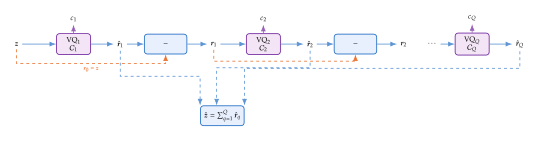
Residual Vector Quantisation (RVQ) elegantly solves this problem by decomposing the quantisation into a cascade of stages, each quantising the residual left by the previous stages.
Definition 14 (Residual Vector Quantisation).
Let be codebooks, each of size with entries in . The Residual Vector Quantiser operates as follows:
Initialise the residual .
For : enumerate
Quantise the residual: .
Record the code index .
Update the residual: . enumerate
Return the quantised vector .
The output is a sequence of code indices .
Theorem 1 (RVQ Approximation Bound).
Let and let be its RVQ approximation with codebooks, each of size . Define the quantisation gain of stage as the ratio of input energy to residual energy, . Then:
(Monotonicity, under a hypothesis on the codebook.) If , then for that stage, and if for every the residual norms are non-increasing throughout the cascade.
(Exact energy decay.) Provided every is finite and nonzero, (RVQ Error) If in addition for every , this implies the weaker but more familiar product bound (RVQ Error WEAK)
(Rate.) The effective bitrate is bits per frame, growing linearly with the number of quantisation stages.
Proof.
Part 1. By construction , where is the codebook entry nearest to . If then is one of the candidates the nearest-neighbour search ranges over, so . Without that hypothesis the claim is false: a codebook whose entries all have large norm can move further from the origin than it started.
Part 2. By the definition of , . Telescoping from gives directly. For the second claim, note that holds precisely when ; applying it factor by factor to yields .
Part 3. Each of the stages contributes one code index from a vocabulary of size , yielding bits per stage and bits total.
Caution.
Both hypotheses in Theorem 1 bite in practice, and in opposite directions.
Trained codebooks do not contain : it is a wasted entry, and nothing in the training objective puts one there. Monotonicity is therefore an empirical tendency rather than a guarantee, and individual stages do occasionally increase the residual norm, at a rate of a few percent of stage applications in a typical trained codec. The cascade still converges because the average energy falls, which is what part 2 is about.
The hypothesis is the one that is quietly violated by the interesting stages. Early stages of a trained RVQ have gains comfortably above 2 - they are removing the bulk of the energy - but the later stages, which are exactly the ones a designer is deciding whether to pay for, routinely fall to and below. Where they do, does not apply and should not be quoted. Use : it is an identity rather than a bound, it needs no hypothesis on beyond finiteness, and where both apply it is far tighter.
Lemma 1 (Orthogonality of RVQ Residuals).
If the codebooks are optimally adapted to the data distribution, then the quantised vectors and the residuals are uncorrelated at each stage: This is the vector quantisation analogue of the normal equations in least-squares regression: the “prediction” and the “residual” are orthogonal in expectation.
Proof.
For an optimal codebook, each Voronoi cell has its centroid at the codebook entry. That is, for each . By the law of total expectation, . Conditioning on the cell assignment: . Therefore , giving .
Proposition 8 (RVQ Effective Codebook Size).
An RVQ with codebooks of size can represent up to distinct vectors. The effective codebook size grows exponentially with the number of stages while each individual codebook remains tractably small: (RVQ Effective SIZE) For the common setting and , this yields , a codebook that would be completely intractable to train as a single flat quantiser.
Proof.
Each of the stages independently selects one of codebook entries. The number of distinct sums is at most , achieved when no two distinct code sequences produce the same sum. In practice, the residual structure ensures that most code combinations yield distinct vectors, so the effective codebook size is close to the theoretical maximum.
SoundStream
SoundStream [10] was the first neural audio codec to combine a convolutional encoder-decoder with RVQ, establishing the architectural template that EnCodec and DAC would later refine.
Definition 15 (SoundStream Architecture).
SoundStream consists of three components:
An encoder that maps a mono waveform to a sequence of continuous latent vectors of dimension , where and is the total downsampling stride.
A residual vector quantiser with codebooks of size , applied independently to each of the latent vectors. The output is a matrix of codes .
A decoder that reconstructs the waveform from the quantised latent sequence .
The encoder consists of a 1D convolution followed by downsampling blocks, each containing residual units and a strided convolution with stride . The decoder mirrors this structure with transposed convolutions. The total stride is .
Example 6 (SoundStream at 6,kbps).
With ,Hz, total stride , codebook size , and quantisation stages, SoundStream produces frames per second, each represented by codes of bits each. The bitrate is bits per second ,kbps. This is a compression ratio of approximately compared to 16-bit PCM at 24,kHz (384,kbps), yet reconstructed audio is nearly indistinguishable from the original in listening tests.
SoundStream is trained with a combination of reconstruction and adversarial losses: (Soundstream LOSS) where is a multi-resolution STFT loss (Definition 12), and are adversarial and feature matching losses from a wave-based discriminator, and is the codebook commitment loss: (VQ LOSS) with denoting the stop-gradient operator and the commitment cost weight.
EnCodec
EnCodec [24] refines the SoundStream architecture with several improvements: a higher-capacity encoder-decoder, a novel loss balancing mechanism, and support for variable bitrates through codebook dropout.
Definition 16 (EnCodec Architecture).
EnCodec shares the encoder-RVQ-decoder structure of SoundStream but introduces:
Larger model capacity: the encoder and decoder use deeper residual networks with more channels, and the encoder additionally incorporates a two-layer LSTM between the convolutional stack and the quantiser to capture long-range temporal dependencies.
Multi-scale STFT discriminator: instead of a single waveform-domain discriminator, EnCodec uses a complex-valued multi-scale STFT discriminator that operates on both real and imaginary parts of the STFT at multiple resolutions.
Loss balancer: a gradient-balancing mechanism that dynamically rescales loss components to ensure stable training (see Definition 17).
Variable bitrate via codebook dropout: during training, each RVQ stage is randomly dropped with some probability, forcing the decoder to reconstruct from fewer codes. At inference time, the user can truncate the code sequence at any stage to achieve a lower bitrate.
The loss balancer deserves special attention, as it addresses a practical difficulty in training multi-loss systems.
Definition 17 (EnCodec Loss Balancer).
Let be the loss components with target weights . The EnCodec balancer rescales the gradient of each loss component so that its contribution to the total gradient norm is proportional to its weight: (Encodec Balancer) where is the exponential moving average of the gradient norms across all losses, and is a small constant. The total gradient applied to the generator is .
Remark 14.
Without the balancer, a loss component with large gradients (e.g., the adversarial loss during early training) can dominate the parameter update and destabilise training. The balancer normalises each gradient to unit norm and then rescales by the target weight, ensuring that the relative influence of each loss component matches the designer's intention regardless of their absolute magnitudes. This is particularly important for audio codecs, where the reconstruction, adversarial, feature matching, and commitment losses can differ by orders of magnitude.
Example 7 (EnCodec bitrate configurations).
EnCodec supports multiple target bitrates by varying the number of active RVQ stages:
tableEnCodec bitrate configurations at 24,kHz with
, stride (75 frames/s).
Bitrate (stages) Bits/frame Quality 1.5,kbps 2 20 Telephony 3.0,kbps 4 40 Wideband speech 6.0,kbps 8 80 Near-transparent 12.0,kbps 16 160 Transparent 24.0,kbps 32 320 Studio quality
DAC: Descript Audio Codec
The Descript Audio Codec (DAC) [25] pushes neural codec quality further through three innovations: improved codebook learning, the Snake activation function, and a multi-band discriminator.
Definition 18 (Snake Activation).
The Snake activation function is defined as (Snake) where is a learnable frequency parameter. Snake is a periodic nonlinearity that preserves the identity component while adding a sinusoidal perturbation. The frequency controls the period of the oscillation.
Remark 15.
Standard activation functions (ReLU, GELU, SiLU) have no inherent periodic structure. Audio waveforms, by contrast, are dominated by periodic and quasi-periodic components (pitched instruments, vowels, harmonic series). The Snake activation provides a mild inductive bias towards periodicity in the learned features, which DAC's authors found to improve reconstruction quality, particularly for tonal signals such as singing voice and sustained instrument notes. The identity component ensures that the activation can still represent aperiodic signals (noise, transients) without difficulty.
Proposition 9 (Properties of the Snake Activation).
The Snake activation satisfies:
Monotonicity: for all , with equality only when .
Asymptotic linearity: as , ; as , the oscillatory component averages out and .
Periodicity: the deviation from linearity, , has period and amplitude . Raising therefore shortens the ripple and shrinks it at the same time.
Proof.
Part 1. Using , we have . Since , we get .
Part 2. Expanding at and dividing by , so the first neglected term is cubic in and . (There is no term at all: the expansion of contains only even powers, so dividing by leaves only odd ones.) For large , the average value of over a period is , giving .
Part 3. The identity yields , which has period and ranges over .
Definition 19 (DAC Improved Codebook Learning).
DAC improves codebook utilisation through two mechanisms:
Factorised codes: each encoder output is projected to a lower-dimensional space with (typically ) before quantisation. The codebook vectors also live in , and the quantised code is projected back: . This forces the codebook to capture the most important variation in a compressed space, improving utilisation.
-normalised codes: both the encoder output and the codebook entries are projected onto the unit sphere before computing distances: (DAC L2 VQ) This is equivalent to maximising cosine similarity and prevents codebook collapse, where entries drift far from the encoder output distribution.
Example 8 (DAC at 8,kbps).
The 44.1,kHz variant of DAC uses stride , yielding approximately 86 frames per second. With codebooks of size : DAC achieves higher reconstruction quality than EnCodec at comparable bitrates, particularly for music, due to the combination of Snake activations, factorised codebooks, and a multi-band multi-scale discriminator that provides sharper adversarial gradients in different frequency ranges.
Codec Comparison
tab:audiogen:codec-comparison summarises the key design choices across the three major neural audio codecs.
tableComparison of neural audio codec architectures.
All use RVQ with codebooks of size , i.e. 10 bits per
stage per frame, so that every bitrate range in the table is
bits per second and can be
checked against the two rows above it. “MR-STFT” denotes
multi-resolution STFT loss; “MS-STFT-D” denotes multi-scale
STFT discriminator.
Feature SoundStream EnCodec DAC Sample rate 24,kHz 24/48,kHz 16/24/44.1,kHz Stride 320 320 320/512 Frame rate 75,fps 75/150,fps 50/75/86,fps (stages) 4–24 2–32 9–32 Bitrate range 3–18,kbps 1.5–24,kbps 6–24,kbps Encoder LSTM No Yes No Activation ELU ELU Snake Discriminator MSD MS-STFT-D MS+MB-D Codebook learning K-means + EMA EMA Factorised, -norm Loss balancing Manual Balancer Manual Variable bitrate Yes Yes No
The “variable bitrate” row is worth pausing on, because it is easily misread as a minor feature. SoundStream's headline contribution was quantizer dropout: train with a random number of active RVQ stages, and a single set of weights then serves every rate from (3,kbps) to (18,kbps), chosen at inference time. EnCodec adopted the same idea. This is what makes the column and the bitrate column consistent with one another - a single fixed-rate codec could not span a range at all - and it is also why a codec's advertised bitrate is a deployment choice rather than an architectural constant.
Insight.
Neural audio codecs serve a dual purpose in modern audio generation systems. First, they act as compressors, reducing audio to a fraction of its original bitrate for storage and transmission. Second, and more importantly for this chapter, they act as tokenisers that convert continuous audio into discrete token sequences, enabling autoregressive language models to generate audio by predicting code sequences. The quality of the codec directly determines the quality ceiling of the downstream generative model: any artefact introduced during quantisation will persist in the generated audio regardless of how well the language model performs.
Caution.
The codec's training data distribution strongly influences its reconstruction quality across audio types. A codec trained predominantly on speech may introduce artefacts when encoding music, and vice versa. EnCodec and DAC are trained on diverse audio (speech, music, environmental sounds) to mitigate this, but domain-specific fine-tuning can yield significant improvements for specialised applications.
The RVQ Token Structure
The output of an RVQ codec is not a single flat sequence of tokens but a matrix of codes , where is the number of quantisation stages and is the number of time frames. This 2D structure poses a fundamental challenge for autoregressive models, which operate on 1D sequences.
There are three principal strategies for linearising the code matrix:
Flat pattern.
Interleave all codes in raster order: . This yields a sequence of length and preserves all dependencies but requires the model to generate tokens per audio frame, which is slow.
Delay pattern.
Introduced by MusicGen [22], the delay pattern offsets each quantisation level by one time step: level at time is placed at sequence position . This allows parallel prediction of codes at different levels for the same time step, reducing the effective sequence length to while maintaining causal ordering.
Coarse-to-fine.
First generate all codes at level (the coarsest level), then all codes at level conditioned on level 1, and so on. This hierarchical approach (used by MusicLM and VALL-E) decouples the coarse acoustic structure from the fine detail but requires sequential passes through the model.
Remark 16.
The choice of linearisation strategy directly affects generation speed, quality, and the model's ability to capture long-range dependencies. The flat pattern is the most expressive but the slowest; the delay pattern offers a practical compromise; the coarse-to-fine approach can leverage specialised models for each level but introduces a cascading error risk (errors at coarse levels propagate to all finer levels). We revisit these tradeoffs in detail when we study autoregressive generation in Autoregressive Music Generation and subsequent sections.
Training Neural Audio Codecs: A Unified View
All three codecs (SoundStream, EnCodec, DAC) share a common training framework that combines four families of loss functions. We consolidate these here to provide a unified perspective.
Definition 20 (Neural Audio Codec Training Objective).
A neural audio codec with encoder , RVQ , and decoder is trained by minimising (Codec FULL LOSS) where:
is a reconstruction loss in the time and/or spectral domain (multi-resolution STFT loss, mel-spectrogram loss, or waveform loss).
is an adversarial loss from one or more discriminators (MPD, MSD, multi-scale STFT discriminator, or multi-band discriminator).
is a feature matching loss computed over intermediate discriminator activations.
is a commitment loss that regularises the encoder outputs to stay close to the codebook entries, ensuring stable quantisation.
The weights control the relative influence of each component. In EnCodec, these are managed dynamically by the loss balancer (Definition 17).
Proposition 10 (Straight-Through Estimator for RVQ).
The vector quantisation operation is piecewise constant and therefore has zero gradient almost everywhere. To enable gradient-based training, the straight-through estimator (STE) replaces the gradient of the quantisation operation with the identity: (STE) where is the identity matrix. In the forward pass, ; in the backward pass, gradients flow through as if . For RVQ with stages, applying the STE at each stage independently gives, for the cascade as a whole, (STE RVQ Total) independently of . The per-stage identities do not accumulate: only the first stage passes gradient to , and every later stage contributes exactly zero. No normalisation by is needed, and none is applied by SoundStream, EnCodec or DAC, all of which implement the cascade as , whose derivative is by inspection.
Proof.
At each stage , the forward computation is and , and the STE sets . Since , the chain rule gives and hence This is the crux: the STE makes the first stage's output track exactly, so the residual it leaves behind has no first-order dependence on at all. Everything downstream inherits that. Formally, suppose for some . Then By induction for every , and summing over stages leaves .
Remark 17.
It is worth being explicit about why the natural guess - stages, each contributing an identity - is wrong. The identities are derivatives with respect to different inputs: , not . Chaining them back to passes through , which the first stage has already annihilated. The result is reassuring rather than surprising: the STE is meant to make the whole quantiser look like a no-op to the backward pass, and a no-op has Jacobian whatever is. A codebook with more stages should not silently multiply the encoder's effective learning rate.
Remark 18.
An alternative to gradient-based codebook learning is the exponential moving average (EMA) update rule. For each codebook entry , let denote the set of encoder outputs assigned to in the current mini-batch. The EMA update is (EMA Count) where is the decay rate (typically ). This rule moves each codebook entry towards the centroid of its Voronoi cell, analogous to the M-step of the k-means algorithm. EMA updates are used by both SoundStream and EnCodec: SoundStream initialises each codebook by running k-means on the first training batch and then maintains it with the EMA rule above, and EnCodec inherits that scheme. DAC is the exception; it learns its codebooks by gradient descent on the commitment and codebook losses, relying instead on the factorised, -normalised parameterisation of Definition 19 to keep them well used.
Insight.
A persistent challenge in training VQ and RVQ systems is codebook collapse: a large fraction of codebook entries receive no assignments and become “dead codes” that contribute nothing to reconstruction quality. Strategies to combat collapse include:
Codebook reset: periodically reinitialise dead entries by sampling from the current batch of encoder outputs.
EMA updates: the smoothing effect of EMA prevents codebook entries from drifting far from the data distribution.
Factorised codes (DAC): projecting to a lower-dimensional space before quantisation concentrates the effective distribution, making it easier for all entries to receive assignments.
normalisation (DAC): constraining both codes and encoder outputs to the unit sphere prevents the distance scale from growing unboundedly, which is a common cause of collapse in high dimensions.
In well-tuned systems, codebook utilisation exceeds 99%, meaning that virtually all entries are actively used during encoding.
From Codecs to Generation
With the codec machinery in place, we can now see how the full audio generation pipeline works in practice. The two-stage paradigm, adopted by virtually all modern systems, is straightforward:
Algorithm 2 (Two-Stage Audio Generation via Neural Codecs).
Stage 1 (Generative model): Given a conditioning signal (text, melody, image, etc.), generate a code matrix using a generative model (autoregressive language model, diffusion model, or flow matching model).
Stage 2 (Codec decoder): Pass through the pretrained codec decoder to obtain the waveform: (TWO Stage Decode)
The generative model never sees raw audio; it operates entirely in the discrete token space defined by the codec. The codec decoder is frozen after pretraining and serves as a universal “audio renderer.”
Remark 19.
Freezing the codec decoder during generation has an important consequence: any quantisation artefacts present in the codec's reconstruction become permanent features of the generated audio. This creates a strong incentive to train the highest-quality codec possible, even if the generative model itself is relatively simple. It also means that improvements to the codec (e.g., upgrading from EnCodec to DAC) can improve generation quality without retraining the generative model, provided the new codec uses a compatible tokenisation scheme.
Example 9 (End-to-end latency analysis).
Consider generating 10 seconds of music at 24,kHz using an autoregressive model over EnCodec tokens with stages and the delay pattern. The effective sequence length is tokens. At an autoregressive generation speed of 100 tokens per second (typical for a 1B parameter transformer with KV-cache on a modern GPU), generation takes approximately 7.6 seconds. The codec decoding step adds negligible overhead (under 50,ms for 10 seconds of audio). The total time is thus dominated by the autoregressive generation, which achieves a real-time factor of approximately .
The sections that follow will develop each generative paradigm in detail: contrastive pretraining for conditioning (CLAP: Contrastive Language–Audio Pretraining), autoregressive generation over codec tokens, latent diffusion over continuous representations, and flow matching for efficient synthesis. In each case, the codec (or, alternatively, a continuous autoencoder) provides the compressed representation that makes generation tractable.
Exercises
Exercise 1 (STFT resolution tradeoff).
Consider an audio signal sampled at ,Hz.
Compute the frequency resolution and the temporal resolution for the following STFT configurations:
Overlap 256 64 75% 1024 256 75% 4096 1024 75% Show that is constant for a fixed overlap ratio, and explain why this reflects an uncertainty principle for time-frequency analysis.
For a music generation system that must faithfully represent both sharp drum transients (requiring fine temporal resolution) and low bass notes at 40,Hz (requiring fine frequency resolution), argue that no single STFT configuration suffices, motivating the multi-resolution approach of Definition 12.
Exercise 2 (Mel filterbank properties).
Verify that the mel scale (Definition 5) is approximately linear for ,Hz (i.e., for some constant ) and approximately logarithmic for ,Hz (i.e., ). Derive the constants , , and .
The mel filterbank matrix is non-square and non-invertible. Explain why the mapping is lossy, and describe what information is discarded.
Suppose you are designing a mel filterbank for a music generation system operating at ,Hz with , spanning ,Hz to . Compute the number of DFT bins and the bin spacing . The narrowest triangle is the first one, whose support runs from to ; find the largest for which , so that every filter spans at least two DFT bins. Check your answer against the two standard choices and : exactly one of them passes. Why does the constraint bind at the low-frequency end rather than the high?
Exercise 3 (RVQ bitrate and quality).
Consider an RVQ codec operating at sample rate ,Hz with total encoder stride and codebook size .
Derive the frame rate in frames per second, where is the signal duration.
Express the bitrate as a function of the number of RVQ stages , and compute the bitrate for .
Using the energy identity , if the quantisation gain for all stages, compute the fraction of the original signal energy remaining in the residual after stages. Then compute what the weaker product bound would give for the same , and confirm that it is looser by roughly four orders of magnitude. Which of the two is a valid conclusion here, and what hypothesis on decides that? Is the tighter figure consistent with the claim that at yields near-transparent quality?
Explain why doubling from 1024 to 2048 (adding 1 bit per frame per stage) is less cost-effective than adding one more RVQ stage (adding 10 bits per frame) in terms of bitrate utilisation.
Exercise 4 (HiFi-GAN discriminator analysis).
Consider the multi-period discriminator with period applied to a waveform of length . What is the shape of the reshaped 2D input tensor? How many columns and rows does it have?
A pitched instrument plays a note at fundamental frequency ,Hz, sampled at ,Hz. The fundamental period in samples is . Explain why the sub-discriminator with period will “see” a clear pattern related to the fundamental (since ), while will produce a less structured 2D image.
The MSD uses average-pooling by factors of 1, 2, and 4. For the sub-discriminator operating at pooling factor 4, what is the effective sample rate? Which frequency components of the signal are invisible to this sub-discriminator?
Argue that the combination of MPD (with prime periods) and MSD (with dyadic scales) provides feedback about both harmonic structure and broadband spectral shape, covering complementary failure modes of the generator.
Exercise 5 (Snake activation analysis).
The Snake activation (Definition 18) is defined as .
Show that by using the identity . What is the period of the oscillatory component?
Compute and show that it is always positive, proving that Snake is a monotonically increasing function. Why is monotonicity important for an activation function used in a decoder network?
As , show that , recovering a near-linear activation, and identify the coefficient of the term. (Why is there no term?) As , argue informally that the oscillatory component averages out and Snake behaves approximately as .
Consider a 1D convolutional layer with Snake activation modelling a sinusoidal signal . Explain qualitatively why the learnable parameter allows the network to “tune” its internal oscillation frequency to match , providing an inductive bias for periodic signals that standard activations lack.
Exercise 6 (Codec as an information bottleneck).
A neural audio codec with encoder , RVQ, and decoder can be viewed through the lens of the information bottleneck principle. Let denote the input waveform and the discrete code matrix.
Write the codec's objective as a trade-off between minimising reconstruction distortion and minimising the information stored in the codes. How does the number of RVQ stages control this trade-off?
The rate of the codec in bits per second is . For fixed , compare two configurations: (i) stages with , and (ii) stages with . Both achieve bits per frame. Argue, using the structure of RVQ, why configuration (i) allocates more bits to the first (coarsest) stage while (ii) distributes bits more evenly, and discuss which might produce better reconstruction.
The information bottleneck predicts that the optimal codec should discard information in that is irrelevant to perceptual quality. Give two concrete examples of audio information that a good codec should discard (i.e., not encode in ), and two examples of information it must preserve.
CLAP: Contrastive Language–Audio Pretraining
Images have CLIP; audio has CLAP\@. The Contrastive Language–Audio Pretraining framework learns a joint embedding space in which audio signals and their textual descriptions are aligned, enabling zero-shot audio classification, text-to-audio retrieval, and, most importantly for this chapter, conditioning signals for generative models. The conceptual parallel with CLIP is deliberate: both methods train dual encoders with an InfoNCE-style contrastive objective, and both produce embeddings that transfer broadly to downstream tasks.
This section formalises the CLAP objective, describes the encoder architectures, and explains why CLAP embeddings have become the default conditioning representation in modern text-to-audio systems. For a thorough treatment of contrastive losses and divergence measures, we refer the reader to 4.
The Audio–Text Alignment Problem
Consider a dataset of paired examples , where is an audio waveform (or its mel-spectrogram representation ) and is a natural language caption describing the audio content. The audio and text modalities live in fundamentally different spaces: the audio is a continuous, high-dimensional signal with temporal structure, while the text is a discrete sequence of tokens with compositional semantics. The alignment problem asks us to learn a shared representation in which semantically matched audio–text pairs are close and unmatched pairs are far apart.
Definition 21 (CLAP: Contrastive Language–Audio Pretraining).
A CLAP model consists of:
An audio encoder that maps a mel-spectrogram to a unit-normalised embedding .
A text encoder that maps a token sequence to a unit-normalised embedding .
A learnable temperature parameter .
The two encoders are trained jointly so that matched pairs have high cosine similarity while unmatched pairs have low cosine similarity.
The cosine similarity between an audio embedding and a text embedding is (CLAP SIM) where the temperature controls the sharpness of the distribution over similarities. Within a mini-batch of pairs, we form the similarity matrix with entries .
Definition 22 (Symmetric Contrastive Loss).
Let be a mini-batch of matched audio–text embedding pairs with similarity matrix entries as in (CLAP SIM). The CLAP contrastive loss is the symmetric InfoNCE objective: (CLAP LOSS) The first term treats each audio sample as a query and retrieves the correct text from among candidates (audio-to-text direction). The second term reverses the roles (text-to-audio direction).
Expanding the two terms, we recognise them as the negative log-probability of the correct match under two softmax distributions: (CLAP A2T) Both terms are instances of the categorical cross-entropy, where the target is the identity permutation: sample should match sample .
Proposition 11 (CLAP Loss as Mutual Information Bound).
The CLAP contrastive loss provides a lower bound on the mutual information between the audio and text embedding distributions: (CLAP MI Bound) Minimising therefore maximises a lower bound on the mutual information, with the bound becoming tighter as the batch size increases.
Proof.
This follows directly from the analysis of InfoNCE by Oord, Li, and Vinyals (2018). Define the critic and note that the InfoNCE loss with negative samples satisfies The expectation of the first term is bounded below by , giving . The bound is tight when the critic is optimal, .
Remark 20.
The temperature plays a critical role in training dynamics. A small (e.g., ) produces sharply peaked softmax distributions, concentrating gradient signal on the hardest negatives but risking training instability. A large (e.g., ) smooths the distribution, slowing convergence but improving robustness to noisy labels. In practice, CLAP models initialise as a learnable scalar, typically starting at , and clamp it to the range during training to prevent collapse.
Definition 23 (CLAP Score).
Given a trained CLAP model , a set of generated audio samples and the corresponding text prompts , the CLAP score is (CLAP Score) where and are the unit-normalised embeddings of the generated audio and the conditioning text, respectively.
This is a definition, not a result. Each summand is a cosine similarity between unit vectors, so by Cauchy–Schwarz it lies in , and therefore so does their mean; the range is an immediate consequence of normalisation and says nothing about how well the score tracks perceptual alignment. The score attains only when every generated audio embedding coincides with its text embedding, and is when the paired embeddings are orthogonal in the joint space. Orthogonality of one pair of vectors is a geometric statement; it is not the same as the two embeddings being statistically uncorrelated, which would be a claim about an expectation over a distribution of pairs. The same quantity is restated for evaluation purposes in Definition 66, where it is normalised per pair rather than per test set.
Audio and Text Encoders
The two arms of the CLAP architecture can be instantiated with a variety of backbone networks. The key design constraint is that both encoders must produce embeddings of the same dimension , so that cosine similarity is well defined.
Audio encoder.
The audio encoder operates on mel-spectrogram inputs . Several backbone choices have been explored in the literature:
CNN14 (from PANNs): A 14-layer convolutional network originally designed for audio tagging. It processes the mel-spectrogram through a sequence of convolutional blocks with batch normalisation and ReLU activations, followed by global average pooling to produce a fixed-dimensional vector .
HTS-AT (Hierarchical Token-Semantic Audio Transformer): A Swin-Transformer-based architecture that treats the mel-spectrogram as a 2D “image” and applies hierarchical windowed self-attention. The [CLS] token output serves as the audio representation .
HTSAT-BERT hybrid: A variant that combines convolutional feature extraction at early layers with Transformer-based global attention at later layers, seeking to capture both local spectral patterns and long-range temporal dependencies.
After the backbone produces , a learned linear projection maps it to the shared embedding dimension: (CLAP Audio PROJ) The normalisation ensures that all audio embeddings lie on the unit hypersphere .
Text encoder.
The text encoder processes a tokenised caption through a pre-trained language model. Common choices include:
BERT (Bidirectional Encoder Representations from Transformers): The [CLS] token representation from the final Transformer layer is used as .
RoBERTa: An optimised BERT variant with improved pre-training procedures. Like BERT, it produces a [CLS] representation that is projected to the shared space.
GPT-2: For autoregressive text encoders, the embedding of the final token (or a special [EOS] token) serves as the sequence-level representation.
As with the audio side, a linear projection and normalisation map the text representation to the shared space: (CLAP TEXT PROJ)
Key Idea.
Shared space, independent encoders. The CLAP framework places no constraint on the internal architecture of the audio and text encoders; they can use entirely different network families (CNNs for audio, Transformers for text). The only coupling occurs through the contrastive loss, which acts on the final normalised embeddings. This modular design means that either encoder can be replaced or upgraded independently, provided the projection dimensions remain compatible.
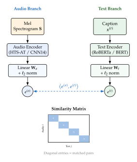
Training Data and Applications
The quality of a CLAP model depends critically on the diversity and scale of its training data. Unlike the image domain, where billions of image–text pairs can be scraped from the web, audio–text pairs are substantially scarcer.
Datasets.
The principal audio-captioning datasets used for CLAP training include:
| Dataset | Clips | Captions/Clip | Source |
| AudioCaps | 50k | 1 | AudioSet subset, human-written |
| Clotho | 6k | 5 | Freesound, crowd-sourced |
| WavCaps | 400k | 1 | ChatGPT-processed web audio |
| LAION-Audio | 630k | 1 | Web-crawled with filtering |
The WavCaps dataset represents an interesting strategy: rather than paying human annotators, the creators used a large language model (ChatGPT) to generate captions from audio metadata and weak labels. This approach trades annotation precision for scale, a trade-off that has proven effective for contrastive pre-training where the loss is robust to moderate label noise.
CLAP for conditioning.
In text-to-audio generation systems, CLAP embeddings serve as the conditioning signal that steers the generative process. Given a text prompt at inference time, the pre-trained text encoder produces , which is then injected into the generative model via cross-attention or FiLM layers (see Conditioning Mechanisms for Audio Generation). This approach decouples the text understanding from the audio generation: the CLAP encoder “understands” the text, and the generative model “creates” the audio.
CLAP for evaluation.
As formalised in Definition 23, the CLAP score measures semantic alignment between generated audio and conditioning text. It has become a standard evaluation metric alongside the Fréchet Audio Distance (FAD) and the Kullback–Leibler divergence over audio event labels. While FAD measures distributional fidelity (how realistic the generated audio sounds), the CLAP score measures prompt adherence (how well the generated audio matches the textual description).
Example 10 (CLAP Score in Practice).
Consider evaluating a text-to-audio model on the AudioCaps test set. For each of the test prompts, the model generates one audio sample. We compute Typical scores for state-of-the-art models (e.g., AudioLDM2, Tango, Make-An-Audio) range from to . As a reference, computing the CLAP score between the ground-truth audio and its caption yields scores around to , reflecting the intrinsic noise in human-written captions that do not capture every acoustic detail.
Historical Note.
The CLAP framework was introduced independently by Wu et al. (2023) and Elizalde et al. (2023), both drawing explicit inspiration from CLIP\@. The name “CLAP” was chosen as a deliberate phonetic echo of “CLIP,” reinforcing the conceptual parallel. Within months of its release, CLAP embeddings became the de facto conditioning signal for nearly every text-to-audio diffusion model, mirroring how CLIP embeddings had become ubiquitous in text-to-image generation.
Autoregressive Music Generation
Diffusion models have dominated recent text-to-audio generation, but an equally powerful paradigm treats audio generation as a language modelling problem. The idea is deceptively simple: tokenise the audio signal into a sequence of discrete codes using a neural codec (see Neural Audio Codecs), then train a Transformer to predict these codes autoregressively, one token at a time. The approach inherits the full machinery of large language models: causal attention, nucleus sampling, KV-cache acceleration, and instruction-following via cross-attention to text encoders.
This section traces the evolution from early approaches such as Jukebox to the modern MusicGen framework, focusing on the mathematical challenge of modelling multi-codebook sequences and the computational trade-offs inherent in autoregressive audio generation.
From Jukebox to Modern Autoregressive Models
The Jukebox model (Dhariwal et al., 2020) was a landmark demonstration that autoregressive Transformers could generate minutes of coherent music with vocals, instruments, and stylistic variation. As discussed in Case Study: Jukebox and Music Generation, Jukebox used a hierarchical VQ-VAE to compress raw audio waveforms into discrete tokens at multiple temporal resolutions, then trained separate autoregressive Transformers at each level of the hierarchy.
While Jukebox proved the concept, it suffered from severe practical limitations. Generating a single minute of music required hours of computation on high-end GPUs, because the VQ-VAE tokens operated at relatively high temporal rates (e.g., one token per waveform samples at the finest level), producing extremely long sequences. The hierarchical generation scheme also introduced error accumulation: artefacts at coarse levels propagated and amplified through finer levels.
The shift to neural codec tokens (from EnCodec, SoundStream, and related models) resolved much of this inefficiency. Neural codecs compress audio far more aggressively than the VQ-VAE approach used by Jukebox, producing token rates of – tokens per second at each codebook level rather than thousands of tokens per second. However, neural codecs introduce a new challenge: the residual vector quantisation (RVQ) scheme produces multiple parallel codebooks, and the autoregressive model must decide how to serialise these multi-codebook tokens into a single sequence.
Key Idea.
Flatten the codebook. A neural codec with codebook levels, codebook size and time frames produces a matrix of tokens , where is the code at time step and codebook level . This is the same object introduced in The RVQ Token Structure, whose entries are written ; we keep the level in a superscript here because the level index selects which embedding table is used. An autoregressive Transformer processes a one-dimensional sequence. The central design decision is how to “flatten” the 2D token matrix into a 1D sequence that the Transformer can model effectively.
The Codebook Flattening Problem
Let denote the token matrix produced by a neural codec with time steps, codebook levels and codebook size . The entry is the discrete code assigned to time step at codebook level . The autoregressive model must define a total ordering on these tokens. Three principal patterns have emerged, each with distinct trade-offs in sequence length, modelling fidelity, and generation speed.
Definition 24 (Interleaved Pattern).
The interleaved pattern serialises the token matrix column-by-column within each time step: (Interleaved) The resulting sequence has length . The autoregressive model predicts each code conditioned on all previous codes across all time steps and codebook levels.
The interleaved pattern is the most faithful to the true joint distribution: it makes no conditional independence assumptions, since each token is conditioned on the complete history. However, the -fold increase in sequence length directly translates to -fold slower generation and -fold higher memory consumption for the KV-cache.
Definition 25 (Delayed Pattern).
The delayed pattern introduces a stagger: codebook level is shifted forward by time steps relative to the first codebook. At each autoregressive step , the model predicts the tokens (Delayed) where tokens with non-positive time indices are masked. The effective sequence length is , and at each step, the model predicts tokens in parallel (one per codebook).
The delayed pattern exploits the observation that the coarser codebook levels () carry the most information about the audio structure, while finer levels () refine acoustic details that depend primarily on the coarse codes at nearby time steps. By delaying finer codebooks, the model ensures that when predicting , it has already seen from the same time step, as well as all codes from earlier time steps. It is worth being precise about when those tokens appear: by (Delayed), the level- code of frame is emitted at autoregressive step , so the frame- codes are emitted at steps respectively - one per step, not all at step . A single frame of the code matrix is therefore completed only after consecutive steps, which is exactly why the schedule costs extra steps in total.
Definition 26 (Parallel Pattern).
The parallel pattern predicts all codes simultaneously at each time step: (Parallel) The effective sequence length is . The model uses independent prediction heads, one per codebook level, and samples all codes in a single forward pass per time step.
The parallel pattern is the fastest at generation time but makes a strong conditional independence assumption: given the past, the codes at time are predicted independently. This ignores the hierarchical dependency structure of RVQ, where finer codes depend on the residual left by coarser codes.
Proposition 12 (Sequence Length Comparison).
For a neural codec with time steps and codebook levels, the effective autoregressive sequence lengths under the three patterns are:
| Pattern | Seq. Length | Tokens/Step | Inter-CB Dep. |
| Interleaved | Full | ||
| Delayed | Partial (delayed) | ||
| Parallel | None (independent) |
Proof.
The interleaved pattern places all tokens in a single sequence with one token per step, giving length . The delayed pattern aligns codebook with a delay of steps; the last codebook () requires additional steps beyond the steps needed for , giving a total of steps. At each step, the model predicts one token per codebook (those that are “active” at that step), for a maximum of tokens per step. The parallel pattern collapses all codebooks into a single step per time index, giving length with tokens per step.
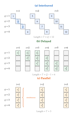
MusicGen: Architecture and Training
MusicGen (Copet et al., 2023) is the most prominent example of a modern autoregressive music generation system built on neural codec tokens. It uses EnCodec as its audio tokeniser and a decoder-only Transformer with the delayed pattern as its core generation engine.
Token representation.
MusicGen operates on EnCodec tokens at kHz with codebook levels and a frame rate of Hz (one frame per ms). Each codebook has entries. A -second music clip is thus represented as a token matrix .
Under the delayed pattern (Definition 25), the autoregressive sequence has length . At each step , the model predicts four tokens (one per codebook level) in parallel, with codebook predicting the token for time step .
Transformer architecture.
The MusicGen Transformer is a standard decoder-only architecture with causal self-attention, as studied in 17. The model uses layers, hidden dimension , attention heads, and a context length of tokens. At each position, the input to the Transformer is the sum of codebook embeddings: (Musicgen Input) where is the embedding matrix for codebook , is a one-hot vector for code , and is the positional embedding for step .
Text conditioning.
MusicGen uses a pre-trained T5 encoder to convert text descriptions into a sequence of conditioning embeddings. These are injected into the Transformer via cross-attention at every layer. Let denote the hidden states at layer and the T5 embeddings projected to dimension . The cross-attention operation at each layer is (Musicgen Crossattn) where , , , and is the per-head dimension. This follows the standard cross-attention mechanism studied in Conditioning Mechanisms.
Melody conditioning via chromagram.
A distinctive feature of MusicGen is its ability to condition on a reference melody. The melody is represented as a chromagram, which encodes the distribution of musical pitch classes over time.
Definition 27 (Chromagram).
Given an audio signal with short-time Fourier transform , the chromagram is a matrix defined by (Chromagram) where indexes the time frame, indexes the pitch class (C, C, D, , B), and (Chroma Pitch) maps frequency bin (with centre frequency ) to its pitch class relative to a reference frequency (typically Hz for A4). The offset of is what makes correspond to C: the note A has pitch-class index in the ordering above, so a semitone count measured from A4 must be shifted by to place the origin on C\@. Without the offset, would name A rather than C, contradicting the labelling. Rounding rather than flooring centres each pitch class on its nominal frequency, so that a bin one quarter-tone sharp of A still maps to A\@.
The chromagram captures harmonic content while being invariant to timbre, dynamics, and instrumentation. Two performances of the same melody on different instruments will produce similar chromagrams. MusicGen discretises the chromagram by taking, at each frame, the over the twelve pitch-class bins (after suppressing the percussive component of the signal), which yields one dominant pitch-class index per frame. This index sequence is embedded and provided to the Transformer as an additional conditioning signal alongside the text embeddings. No separate learned codebook is involved: the “quantisation” is the argmax over an existing twelve-way axis, and keeping only the dominant bin is deliberate, since retaining the full chroma vector lets the model copy the reference almost verbatim rather than treating it as a melodic constraint.
Algorithm 3 (MusicGen Generation with Delayed Pattern).
Input: Text prompt , optional melody audio , number of time steps , temperature , codebook levels . Output: Generated audio waveform .
Encode conditioning: enumerate
Compute text embeddings: .
If melody provided, compute chromagram: and quantise to melody tokens. enumerate
Initialise: Set (empty token matrix). Initialise KV-cache.
Autoregressive loop: For : enumerate
Compute input embedding from active tokens using (Musicgen Input).
Run Transformer forward pass with cross-attention to (and melody tokens if present).
For each codebook where and : enumerate
Compute logits .
Sample . enumerate
Append sampled tokens to and update KV-cache. enumerate
Decode: Convert token matrix to waveform using the EnCodec decoder: .
Remark 21.
MusicGen applies classifier-free guidance (CFG) during generation. During training, the text conditioning is dropped with probability , replacing the T5 embeddings with a learned null embedding. At inference, the logits are interpolated: where is the guidance scale (typically ). This doubles the cost per step (two forward passes), but substantially improves text adherence. See Classifier-Free Guidance for Audio for a detailed treatment of CFG for audio.
Example 11 (MusicGen Token Rates).
Consider generating seconds of music at kHz. The EnCodec tokeniser operates at Hz with codebook levels, producing time frames. The delayed pattern requires autoregressive steps. With a Transformer that processes each step in approximately ms (including KV-cache update and two forward passes for CFG), the total generation time is seconds. This achieves roughly real-time generation on a modern GPU, a dramatic improvement over Jukebox's hours-per-minute rate.
For comparison, the interleaved pattern would require steps, taking approximately seconds and consuming more KV-cache memory.
The Autoregressive Bottleneck
Despite the improvements brought by neural codecs and the delayed pattern, autoregressive audio generation faces a fundamental computational bottleneck: generation is inherently sequential. Each token depends on all previously generated tokens, so the model must be evaluated once per time step, with no opportunity for temporal parallelism during inference.
Sequential generation speed.
For a sequence of length , autoregressive generation requires forward passes through the Transformer. With a KV-cache, each forward pass processes a single new position, so its cost scales as , where is the model dimension and is the current cache length. Summing over the steps, during which the cache grows from to , gives a total of (AR COST Order) It is worth reading this expression carefully, because it is easy to mislabel it as “quadratic in the sequence length”. The two terms are of comparable size only when ; below that the linear term dominates and the total cost is, to a good approximation, linear in . With the constants worked out in Proposition 13, the crossover for the MusicGen configuration () sits at tokens, which is more than eight minutes of audio at Hz. For all sequence lengths of practical interest in this chapter the quadratic attention term is a correction, not the leading cost.
Proposition 13 (Autoregressive Generation Cost).
Let be the autoregressive sequence length, the model dimension, the number of attention heads and the number of Transformer layers. The total floating-point operations for generating one complete sequence (using KV-cache) is (AR COST) where is the average cache length across all steps (since the cache grows from to ). For a generation batch of size the cost is times this.
Proof.
At step , the KV-cache has entries. Attention against the cache costs two matrix products, not one: the query–key dot products cost FLOPs per layer (for heads, each of dimension , the total is still ), and forming the attention-weighted sum of the cached value vectors costs a further , for in all. The QKV projections and output projection each cost FLOPs per layer (four projections total: ). The FFN with hidden dimension costs FLOPs. Summing over steps and layers, with the attention term averaging to , gives the stated expression.
Remark 22 (Reading the cost formula).
(AR COST) is a sum of a term linear in and a term quadratic in , and the quadratic term carries the much smaller constant. The two are equal when , that is at ; for MusicGen's this is tokens. Below that crossover, doubling the sequence length costs rather less than double, and the naive expectation that “cost is quadratic in ” badly overstates the penalty for longer audio. Concretely, with and , moving from the delayed pattern's to the interleaved pattern's multiplies the sequence length by and the FLOP count by only - not by the that a purely quadratic reading would predict. The quadratic term does eventually bite, and it is the reason long-form generation in Long-Form Audio and Music Generation needs more than a bigger context window; but it bites at minutes of audio, not at seconds.
KV-cache memory.
The KV-cache stores the key and value tensors for all previous positions, consuming (KV Memory) bytes. For MusicGen's configuration (, , , ), this is bytes per batch element, that is MiB (equivalently MB in decimal units - the distinction matters when the two are within ten per cent of a device's memory budget). Generating long audio clips (e.g., minutes) would require , pushing KV-cache memory to GiB ( GB) per sample. For a treatment of memory-efficient attention mechanisms that can mitigate this cost, see 24.
Insight.
The speed–fidelity–length trilemma. Autoregressive audio models face a three-way trade-off: (i) faster generation (parallel or delayed patterns) sacrifices inter-codebook modelling fidelity; (ii) higher fidelity (interleaved pattern) requires longer sequences and slower generation; (iii) longer audio clips demand proportionally more computation and memory, regardless of the pattern choice. Diffusion-based approaches (Spectrogram-Domain Generation) offer an alternative that parallelises across the time dimension, but introduce their own trade-offs in iterative denoising cost.
Conditioning Mechanisms for Audio Generation
A generative model that produces audio unconditionally is of limited practical use: we nearly always want to control what is generated. The conditioning signal might be a text description (“a jazz piano solo with brushed drums”), a melody hummed by the user, a chord progression, song lyrics, a reference audio clip whose style should be transferred, or even a video whose soundtrack must be synchronised.
This section catalogues the principal conditioning modalities for audio generation, then analyses the mathematical mechanisms through which conditioning information is injected into the generative model. Many of these mechanisms are shared with image and video generation (Conditioning Mechanisms); here we focus on the adaptations and considerations specific to the audio domain.
The Conditioning Landscape
Table 1 summarises the principal conditioning modalities used in modern audio generation systems.
| Modality | Representation | Control Level | Example Systems |
| Text description | CLAP / T5 embeddings | Semantic | MusicGen, AudioLDM2 |
| Melody | Chromagram tokens | Pitch contour | MusicGen (melody mode) |
| Chords | Chord sequence embeddings | Harmonic structure | SingSong, Jukebox |
| Lyrics | Phoneme / text alignment | Vocal content | Jukebox, VoiceCraft |
| Audio reference | Codec / CLAP embedding | Style / timbre | MusicLM, AudioLDM |
| Video | CLIP / temporal features | Temporal sync | SpecVQGAN, Diff-Foley |
| MIDI | Discrete note events | Note-level control | MIDI-DDSP |
The richness of this conditioning landscape is a distinguishing feature of audio generation compared to image generation, where text is the dominant conditioning modality. In audio, the temporal structure of the output creates opportunities for temporally aligned conditioning signals (melody, chords, lyrics, video) that have no direct analogue in the image domain.
Cross-Attention Conditioning
Cross-attention is the most common mechanism for injecting conditioning information into Transformer-based audio generators. The mechanism is identical in form to the cross-attention used in image and video diffusion models (Conditioning Mechanisms), but the conditioning and generation modalities differ.
Definition 28 (Cross-Attention Conditioning for Audio).
Let denote the hidden states of the audio generation model (either an autoregressive Transformer or a diffusion model's denoiser) and let denote the conditioning embeddings (e.g., from a T5 or CLAP encoder), projected to dimension by a linear map acting on the right, so that . The cross-attention output is (Crossattn) where are the query, key, and value projection matrices for a single attention head, and is the per-head dimension. The multi-head version concatenates such heads and applies an output projection.
The attention weights form a soft alignment matrix between the audio generation positions and the conditioning positions. Each row of is a probability distribution over the conditioning tokens, determining how much each conditioning token influences the corresponding audio generation position.
Remark 23.
In text-to-audio generation, the cross-attention weights provide an interpretable window into how the model uses the text prompt. Visualising often reveals that the model learns to attend to relevant words at appropriate times: for example, when generating the drum section of a prompt like “jazz piano followed by drum solo,” the cross-attention weights shift from the word “piano” to the word “drum” at the transition point. This emergent temporal alignment arises without any explicit alignment supervision.
Proposition 14 (Cross-Attention as Conditional Expectation).
The cross-attention output at position can be written as a conditional expectation under a learned distribution: (Crossattn Expectation) where and . The output is therefore the expected value of the conditioning representation under a soft retrieval distribution, where the query at position determines which conditioning tokens are most relevant.
Proof.
The result follows immediately from the definition of softmax attention. The attention weights and , so they define a categorical distribution over conditioning positions . The weighted sum is the expectation of the random variable where .
FiLM Conditioning
Feature-wise Linear Modulation (FiLM) provides a computationally efficient alternative to cross-attention for injecting conditioning information. Rather than attending to a sequence of conditioning tokens, FiLM conditions by applying a learned affine transformation to the hidden features.
Definition 29 (FiLM: Feature-wise Linear Modulation).
Let be a hidden feature vector at any position in the generation model, and let be a global conditioning vector (e.g., a CLAP embedding or a time-step embedding). The FiLM transformation is (FILM) where denotes element-wise multiplication, and the scale and shift parameters are generated from the conditioning vector: (FILM Params) with and being learnable parameters.
The FiLM mechanism is closely related to the Adaptive Layer Normalisation (AdaLN) used in diffusion Transformers. In AdaLN, the affine parameters of layer normalisation are conditioned on the time step and class label; FiLM generalises this to arbitrary conditioning signals.
Proposition 15 (FiLM as Conditional Affine Transform).
The FiLM transformation is a conditional affine transformation of , parameterised by the conditioning vector . Specifically, it can be written as (FILM Affine) where is a diagonal matrix and is a bias vector, both dependent on . The transformation is linear in for fixed , but nonlinear in when composed with subsequent nonlinear layers.
Proof.
Expanding the element-wise product: Therefore , and . Substituting gives , and similarly for .
Remark 24.
FiLM and cross-attention represent two extremes of the complexity–expressivity spectrum for conditioning:
FiLM uses a global conditioning vector that applies the same affine transformation at every position. It cannot perform position-dependent conditioning (e.g., different instruments at different times) unless the conditioning vector itself encodes temporal information.
Cross-attention uses a sequence of conditioning tokens and learns position-dependent alignment via attention weights. It is strictly more expressive but requires computation.
In practice, many audio generation architectures use both: FiLM for global conditioning (e.g., diffusion time step, global style) and cross-attention for sequential conditioning (e.g., text tokens, melody).
Classifier-Free Guidance for Audio
Classifier-free guidance (CFG) was originally developed for class-conditional image generation and later extended to text-to-image and text-to-video diffusion models (see Classifier-Free Guidance for Video). Its application to audio generation follows the same mathematical framework, but the practical considerations differ in important ways.
Review of CFG.
During training, the conditioning signal is dropped with probability (typically to ), replaced by a null conditioning token . At inference, the model's output (score function, velocity field, or logits, depending on the generative framework) is extrapolated along the conditioning direction: (CFG) where is the guidance scale. Note the convention: makes (CFG) collapse to , that is to ordinary conditional generation with no guidance at all; it is that would recover the unconditional prediction . Increasing above extrapolates past the conditional prediction, amplifying the influence of the conditioning signal at the cost of reduced sample diversity.
Caution.
Two guidance conventions. Much of the image-generation literature and most user-facing tools report a single “guidance scale” defined by , which is (CFG) with . Under that convention the no-guidance point is , not . Whenever a guidance number is quoted without its defining equation, check which of and is meant: the commonly cited image range of to is a range of , and corresponds to in (CFG). We use throughout this chapter.
Audio-specific guidance scales.
A notable empirical observation is that the optimal guidance scales reported for audio generation are lower than those reported for image generation. Part of that gap is bookkeeping rather than substance: the image figures usually quoted, to , are values of and so correspond to , which shrinks the apparent gap to roughly a factor of two to three. The remainder is real, and reflects how audible over-guidance is: the artefacts catalogued at the end of this subsection (harmonic distortion, spectral peaking, temporal repetition) appear at guidance strengths that would still look benign in an image. Text-to-audio systems therefore operate in the range , with the precise choice depending strongly on the task; Remark 38 gives per-task figures, from for speech up to for music.
It is tempting to explain the audio/image difference by observing that audio captions are vaguer than image prompts (“birds singing near a stream” versus “a red car parked on a snowy street”). That observation is correct, but it does not by itself settle the direction of the effect, and the reader should be wary of it: vagueness can be read as leaving room for perceptually valid variation, hence arguing for less guidance, or as under-determining the target, hence arguing for more. Both readings appear in the literature. What the evidence actually supports is the narrower claim above - that audio degrades audibly at lower guidance strengths than images degrade visibly - together with the per-task ordering in Remark 38, in which the tasks with the most intrinsic structure (speech) tolerate the least guidance.
Definition 30 (Audio CFG with Scale Schedule).
For diffusion-based audio generation with denoising steps, a guidance scale schedule specifies a potentially time-varying guidance scale: (CFG Schedule) A common schedule uses higher guidance at early (noisier) denoising steps and lower guidance at later (less noisy) steps: for some power .
Caution.
Over-guidance distortion in audio. When the guidance scale is too high, audio generation models produce characteristic distortion artefacts that differ from the over-saturation seen in images. In audio, excessive guidance manifests as: (i) harmonic distortion, where pure tones acquire unnatural overtones; (ii) spectral peaking, where energy concentrates in narrow frequency bands, producing a “metallic” or “synthetic” quality; (iii) temporal repetition, where the model becomes trapped in repetitive patterns, sacrificing temporal variation for prompt adherence. These artefacts are particularly severe for music generation, where the listener has strong expectations about spectral smoothness and temporal dynamics. As a rule of thumb, if the generated audio sounds “overcooked” or unnatural, reducing the guidance scale by – points is the first intervention to try.
Proposition 16 (CFG as Posterior Sharpening).
Under the score-based interpretation, the guided score corresponds to sampling from a distribution proportional to (CFG Sharpened) which is the unconditional distribution reweighted by the -th power of the likelihood ratio. When , this sharpens the conditional distribution, concentrating mass on regions of -space where the conditioning signal is most probable.
Proof.
The unconditional and conditional scores are and , respectively. By Bayes' rule, The CFG score is This is the score of the distribution , which can be rewritten as . Since is a constant with respect to , the normalised distribution is .
Multi-Modal Conditioning
Real-world audio generation tasks often require simultaneous conditioning on multiple modalities. A user might specify a text description (“upbeat pop song”), provide a melody (hummed reference), and indicate a desired style (audio of a reference track). The generation model must fuse these heterogeneous signals into a coherent conditioning representation.
Conditioning fusion strategies.
Three principal strategies exist for combining multiple conditioning modalities:
Concatenation: The conditioning embeddings from different modalities are concatenated along the sequence dimension before being provided to cross-attention. If the text embeddings are and the melody embeddings are , the combined conditioning is (Concat COND) The attention mechanism then learns to attend to the appropriate modality at each generation position.
Separate cross-attention: Each conditioning modality is injected through its own cross-attention layer, and the outputs are summed: (Separate Crossattn) This allows independent attention patterns for each modality but increases the parameter count and computational cost.
Hierarchical conditioning: Global conditioning signals (style, genre) are injected via FiLM, while sequential conditioning signals (text, melody) are injected via cross-attention. This leverages the strengths of each mechanism.
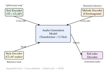
Example 12 (Multi-Modal Conditioning in MusicGen).
MusicGen supports joint text and melody conditioning. The text description is encoded by a T5 model and provided via cross-attention. The melody is represented as a quantised chromagram and provided as an additional conditioning sequence. At each Transformer layer, the model attends to both conditioning sequences: In practice, the melody conditioning is found to strongly constrain the pitch contour of the generated music, while the text conditioning influences instrumentation, genre, and mood. The model learns to balance these signals without explicit weighting.
Lemma 2 (Additivity of Separate Cross-Attention).
The separate cross-attention approach in (Separate Crossattn) implicitly assumes that the conditioning modalities contribute additively to the hidden representation. Formally, let and . Then (Additive COND) neglects any interaction terms between the two modalities. An interaction-aware formulation would require joint attention over the concatenated conditioning sequence, as in (Concat COND).
The property at issue is additivity of the two conditioning contributions, not conditional independence of the modalities: nothing here asserts that and are independent given anything, and indeed in Example 12 the melody is extracted from audio that the caption also describes, so they are strongly dependent. What the architecture assumes is only that their effects on combine by addition.
Proof.
By construction, the separate cross-attention layers compute their outputs independently: depends on but not on , and vice versa. The sum is therefore a first-order approximation to the joint conditioning effect. In contrast, the concatenation approach allows the attention weights over text tokens to depend on the melody tokens (through the shared softmax normalisation), capturing cross-modal interactions.
Spectrogram-Domain Generation
Before neural codecs and latent diffusion models became the dominant paradigm, an influential line of work explored generating audio by treating mel spectrograms as images and applying image generation techniques directly. This approach, most famously demonstrated by Riffusion, is conceptually elegant: it repurposes the extensive machinery developed for image synthesis (U-Net denoisers, latent diffusion, classifier-free guidance) without any audio-specific architectural modifications.
This section analyses the mathematics of spectrogram-domain generation, its surprising effectiveness, and the fundamental limitations that ultimately motivated the shift to latent codec spaces.
Riffusion: Image Diffusion Meets Audio
Riffusion (Forsgren and Martiros, 2022) was a proof-of-concept demonstration that fine-tuning Stable Diffusion on mel spectrogram images could produce musically coherent audio. The approach consists of three stages:
Data preparation. Each audio clip is converted to a mel spectrogram , which is then rescaled and formatted as a single-channel (or three-channel, with the spectrogram duplicated) image of fixed resolution (e.g., ).
Fine-tuning. The pre-trained Stable Diffusion model, including its latent autoencoder and U-Net denoiser, is fine-tuned on the spectrogram “images” with corresponding text captions. The VAE encoder learns to compress spectrograms into the same latent space, and the U-Net learns to denoise spectrograms rather than natural images.
Inversion. The generated spectrogram is converted back to a waveform using a spectrogram inversion algorithm (e.g., Griffin–Lim or a neural vocoder such as HiFi-GAN).
Insight.
Reusing image priors for audio. The remarkable finding of Riffusion is that the visual priors learned by a model trained on natural images (smooth textures, coherent structures, sharp edges) transfer meaningfully to mel spectrograms. Harmonic sounds appear as horizontal lines in the spectrogram (analogous to edges in images), percussive sounds appear as vertical lines (analogous to vertical edges), and gradual timbral changes appear as smooth texture variations. The pre-trained image model already “knows” how to generate coherent visual structures; it merely needs to learn the specific visual vocabulary of spectrograms.
Formally, the Riffusion generation process can be described as follows. Let and denote the pre-trained (and fine-tuned) Stable Diffusion VAE encoder and decoder, and let be the fine-tuned U-Net denoiser. Given a text prompt , the generation pipeline is: (Riffusion Sample) where is the generated mel spectrogram and is the reconstructed waveform.
Example 13 (Riffusion Spectrogram Generation).
Consider generating a -second audio clip at kHz with a hop size of samples and mel frequency bins. The mel spectrogram has dimensions time frames and frequency bins. After zero-padding to (to match Stable Diffusion's expected input resolution), the spectrogram is treated as a single-channel image.
The Stable Diffusion VAE compresses this to a latent tensor of shape (with spatial downsampling), and the U-Net performs denoising in this latent space. Counting values, the compression ratio is .
This is not the ratio the same encoder achieves on the natural images it was trained for: an RGB image carries three channels, so there the ratio is , three times larger. A single-channel spectrogram is already a third as large going in, and the VAE spends its full four-channel latent budget on it. The spatial downsampling factor of is what is shared between the two cases; the value-count ratio is not. If the spectrogram is replicated across three channels to match the encoder's expected input - which is what Riffusion actually does - the input value count is again and the nominal ratio returns to , but two of the three channels are exact copies, so the information-bearing compression is still .
Proposition 17 (Spectrogram Image Diffusion Equivalence).
Let be a U-Net denoiser trained on natural images and let be the same architecture fine-tuned on mel spectrograms (with channel replication to match the 3-channel input). The fine-tuned model minimises the same denoising objective: (SPEC Image Equiv) The only difference from the image training objective is the data distribution: spectrograms replace natural images. All mathematical properties of DDPM (convergence guarantees, score matching equivalence, the connection to SDEs) transfer without modification.
Proof.
The DDPM framework is defined for arbitrary data distributions on and does not depend on the data being images. The forward process is well defined for any . The denoising score matching objective is a proper scoring rule for estimating the score regardless of the underlying data distribution. Therefore, the mathematical framework applies verbatim, and the only effect of changing the data domain is on the learned function .
Spectrogram-to-waveform inversion.
The critical step in the Riffusion pipeline is converting the generated mel spectrogram back to a waveform. This inversion is inherently ill-posed: the mel spectrogram discards phase information and compresses the linear frequency axis, so multiple waveforms can produce the same mel spectrogram.
The classical approach is the Griffin–Lim algorithm, which iteratively searches for a phase field consistent with the given magnitudes by alternating between the time-domain and frequency-domain constraints. Starting from a random phase estimate , the algorithm iterates: (Griffin LIM) where is the magnitude spectrogram (obtained by inverting the mel filterbank) and denotes the phase angle. After iterations (typically to ), the reconstructed waveform approximately satisfies the magnitude constraints.
It is important to be clear about what this procedure does and does not achieve. Each iteration monotonically decreases the inconsistency between and the STFT of its own overlap-added inverse, and that is the only quantity it decreases. It does not decrease the distance to the original phase, and in general it does not recover it. Running the iteration on a signal whose true phase is known makes the point sharply: the magnitude error falls by an order of magnitude while the phase error of Definition 32 stays pinned at the value a uniformly random phase would score. Griffin–Lim converges to a consistent phase, not the phase; the resulting waveform has roughly the right spectral envelope and the wrong fine structure, which is exactly what the characteristic “phasiness” of Griffin–Lim output sounds like.
Modern systems replace Griffin–Lim with neural vocoders (HiFi-GAN, BigVGAN, Vocos) that directly map mel spectrograms to waveforms using a generative neural network. These produce substantially higher-quality audio, as they learn to predict plausible phase patterns from the spectrogram structure.
Mathematics of Spectrogram Diffusion
When we apply diffusion models to mel spectrograms, the data space is rather than the image space . The forward noising process and reverse denoising process follow the same mathematical framework as image diffusion, but the structure of the data introduces domain-specific considerations.
Definition 31 (Spectrogram Diffusion).
Let be a normalised mel spectrogram (treated as a 2D tensor). A spectrogram diffusion model defines a forward process (SPEC Forward) and trains a denoiser to predict the noise component, with loss (SPEC LOSS) where and .
The key question is: what does the denoiser learn about the structure of mel spectrograms? Natural audio spectrograms exhibit a rich set of statistical regularities:
Horizontal continuity: Harmonic components of sustained sounds create horizontal ridges in the spectrogram that persist across many time frames.
Harmonic spacing: A fundamental frequency produces harmonics at , which appear as evenly spaced horizontal lines (on a linear frequency axis) or logarithmically spaced lines (on a mel axis).
Onset transients: Percussive events produce vertical broadband features spanning many frequency bins in a single time frame.
Spectral envelope: The overall energy distribution across frequencies follows smooth, slowly varying envelopes determined by the source and resonance characteristics.
The diffusion model learns these regularities implicitly through the training data. The U-Net architecture is particularly well suited to capturing both local features (individual harmonics) and global structure (musical form, temporal dynamics) through its multi-scale encoder–decoder structure.
Proposition 18 (Spectrogram Grid Density and the Gabor Limit).
Consider a short-time Fourier transform with window length , hop size and sampling rate . Write for the spacing between successive frames (in seconds) and for the spacing between adjacent frequency bins (in Hz). Then:
Grid density. The area of one cell of the time–frequency sampling grid is (SPEC Uncertainty) with equality exactly when , that is when the frames do not overlap. Every overlapping STFT has ; the common choice gives .
Gabor limit. The grid spacings are not the resolution. Writing and for the root-mean-square time and bandwidth spreads (in seconds and Hz) of the analysis window itself, no window achieves a product smaller than (SPEC Gabor) with equality attained only by the Gaussian window ((Gabor Limit)). This is the genuine uncertainty statement, and it constrains the window, not the sampling grid.
Consequently the trade-off is real but is governed by alone: increasing narrows and widens , and vice versa. Decreasing at fixed buys extra samples of the same underlying resolution, not extra resolution.
Proof.
For part 1, the DFT of an -sample window has bins spaced by , and consecutive frames are separated by samples, that is by seconds. Hence and since a usable STFT requires , this quantity lies in and equals precisely at . Note that the cancels, so no choice of sampling rate can move this product; in particular there is no configuration in which it exceeds .
For part 2, (SPEC Gabor) is the Heisenberg–Gabor inequality applied to the analysis window , viewed as a function of time with Fourier transform , and is stated for this chapter in Remark 5. It involves no reference to : overlapping the frames replicates window placements, which changes how densely the plane is sampled but leaves each individual measurement, and therefore and , untouched.
Caution.
Grid spacing is not resolution. It is tempting to write “” by analogy with the uncertainty principle, but as (SPEC Uncertainty) shows this inequality points the wrong way: it would force , which no overlapping STFT satisfies. The quantity that obeys a lower bound is for the window, and its bound is , not . The same relation is derived again in the chapter-level exercises.
Remark 25.
The time-frequency trade-off has direct implications for spectrogram-domain generation. A common configuration for music generation uses samples ( ms at kHz) and samples ( ms), yielding Hz and ms. This provides reasonable resolution for both harmonic analysis and transient detection. For a -second clip, the spectrogram has time frames, which can be unwieldy for diffusion models. Reducing (by increasing ) sacrifices temporal resolution; reducing (by using fewer mel bands) sacrifices frequency resolution. This motivates the use of latent diffusion, which operates on a compressed representation.
Example 14 (Spectrogram Diffusion for Sound Effects).
Consider generating a -second sound effect (“thunderstorm with heavy rain”) using a spectrogram diffusion model. With Hz, , , and mel bins, the spectrogram has shape . After padding to (to be divisible by the U-Net's downsampling factor), the diffusion model operates on a tensor comparable in size to a small image.
The model generates a spectrogram that captures the broadband noise of rain (diffuse energy across all frequencies), the low-frequency rumble of thunder (concentrated energy below Hz), and the temporal dynamics of thunder claps (transient broadband events). The spectrogram is then converted to a waveform using HiFi-GAN, which generates plausible phase information to create a realistic audio signal.
Limitations of Spectrogram-Domain Generation
Despite its conceptual elegance, spectrogram-domain generation suffers from several fundamental limitations that have driven the field toward latent codec spaces.
Phase loss.
The most fundamental limitation is the loss of phase information. A mel spectrogram represents only the magnitude of the STFT, discarding the phase component. This means that the diffusion model generates magnitude-only representations, and the phase must be estimated during the inversion step.
Definition 32 (Phase Reconstruction Error).
Let be a generated mel spectrogram with corresponding ground-truth magnitude spectrogram and phase . Let denote the phase estimated by the inversion algorithm. The phase reconstruction error is (Phase Error) This error is zero when the estimated phase matches the true phase and reaches its maximum of when the phases are perfectly anti-aligned.
A useful reference point on this scale is the value achieved by guessing. If is uniform on then , so is what a phase field carrying no information about the target scores. This is the number to compare against when assessing an inversion algorithm, and, as noted above, it is roughly where Griffin–Lim sits however long it is run.
Even state-of-the-art neural vocoders introduce subtle phase artefacts, particularly in regions of the spectrogram with rapid temporal variation (transients) or closely spaced harmonics. These artefacts manifest as “buzziness,” “phasiness,” or reduced clarity in the reconstructed audio.
Frequency resolution.
The mel frequency scale provides perceptually motivated frequency resolution: high resolution at low frequencies (where pitch perception is acute) and lower resolution at high frequencies (where the ear is less sensitive to fine spectral detail). However, this compression means that the generated spectrogram has limited control over the fine frequency structure of the audio.
Proposition 19 (Mel Frequency Resolution Bound).
For a mel filterbank with filters spanning the frequency range , the frequency resolution at frequency is approximately (MEL Resolution) In particular, is affine in through the factor , so the resolution degrades linearly with frequency. Note that the value depends on the analysis band as well as on , through the logarithm: the same spread over a wider band buys coarser resolution everywhere. At Hz with mel bins covering the full band Hz of kHz audio, Hz; restricting the same bins to Hz sharpens this to Hz. Either way, harmonics closer together than that spacing are merged in the mel representation - which at kHz means the harmonic series of any voice with a fundamental below about Hz is already unresolved.
Proof.
The mel scale maps frequency to . The inverse is . For uniformly spaced mel filters between and , the mel spacing is . The frequency resolution at mel value is . Since , this simplifies to . Converting back to the stated form using , and noting , we obtain .
The approximation sign covers two small effects. First, the derivative is evaluated at a point rather than integrated across a band, which is accurate whenever is small compared with the mel range. Second, the filterbank of Definition 6 places centre frequencies, so the true centre spacing is rather than the used here, a factor of . At this is a per cent correction: building the filterbank explicitly on Hz gives a measured centre spacing of Hz near kHz against the Hz predicted above.
Limited duration.
Spectrogram-domain generation inherits the resolution constraints of the underlying image generation model. Standard diffusion models operate on fixed-resolution images (e.g., ), which limits the spectrogram to a fixed time–frequency grid. For a hop size of at Hz, a -frame spectrogram represents only seconds of audio. Generating longer clips requires either: (i) sequential generation with overlap and crossfade, which introduces stitching artefacts; or (ii) higher-resolution generation, which is computationally expensive and may not be supported by the architecture.
Remark 26 (Why Modern Systems Moved to Latent Codec Space).
The limitations of spectrogram-domain generation, particularly phase loss, limited frequency resolution, and fixed duration constraints, motivated the development of generation models that operate in the latent space of neural codecs. In a neural codec latent space:
Phase is preserved: The codec encoder and decoder jointly learn to encode and reconstruct the full waveform, including phase information. There is no separate inversion step.
Resolution is adaptive: The RVQ codebook captures audio structure at multiple resolution scales through its hierarchical refinement, rather than being fixed by the STFT parameters.
Duration is flexible: Neural codec tokens operate at a fixed temporal rate (e.g., Hz), so longer clips simply produce longer token sequences without changing the frequency resolution.
The transition from spectrogram-domain to codec-domain generation, which occurred rapidly between 2022 and 2023, mirrors the earlier transition from pixel-space to latent-space diffusion in image generation. In both cases, the insight is the same: operate in a learned representation space that captures the essential structure of the data, rather than in a hand-designed representation (spectrograms, pixels) that was not optimised for generation.
Conjecture 1 (Codec Latent Spaces Subsume Spectrogram Spaces).
Let be the manifold of valid mel spectrograms and let be the manifold of neural codec latent embeddings. We conjecture that for a sufficiently expressive codec, captures strictly more information about the audio signal than : where denotes conditional entropy. In other words, the neural codec latent representation leaves less residual uncertainty about the original waveform than the mel spectrogram representation. This conjecture, if true, would formally justify the empirical observation that codec-based generation outperforms spectrogram-based generation.
Historical Note.
Riffusion appeared in late 2022 as an open-source project, not a peer-reviewed paper. Despite its simplicity (or perhaps because of it), the project attracted enormous attention, demonstrating that off-the-shelf image generation models could produce recognisable music with minimal adaptation. The project's name is a portmanteau of “riff” (a musical phrase) and “diffusion.” While Riffusion itself was quickly surpassed by purpose-built audio generation models, it served as an important conceptual bridge, showing the research community that the mathematical framework of diffusion models was not inherently tied to the image domain.
Exercises
Exercise 7 (CLAP Batch Size and Mutual Information).
Consider a CLAP model trained with the symmetric contrastive loss ((CLAP LOSS)).
Show that the audio-to-text loss is bounded below by , and explain why is approached but never attained for finite similarities. Then show that exactly when every row of the similarity matrix is constant ( for all ), where is the batch size.
It is tempting to conclude from part (a) that is an upper bound on . Show that it is not, by exhibiting a similarity matrix with for which . (Hint: take and for ; the loss is then .) Explain in one sentence why the loss is in fact unbounded above, and why is nevertheless the right reference value: it is the loss of an untrained model, whose similarities carry no information.
Using the mutual information bound from Proposition 11, explain why a CLAP model trained with batch size can certify at most nats of mutual information between the audio and text modalities, while raises the ceiling to nats. Be careful to distinguish the ceiling on the bound from a ceiling on the true mutual information, which does not depend on at all. What are the practical implications for audio generation quality?
Suppose the true mutual information between the audio and text distributions is nats. What is the smallest batch size for which the bound of Proposition 11 could certify all of , that is for which is possible in principle? Compute the exact value, and note that this is a necessary condition on , not a sufficient one: attaining it also requires .
Exercise 8 (Codebook Flattening Patterns).
Consider a neural codec with time steps, codebook levels, and codebook size .
Compute the autoregressive sequence length for each of the three flattening patterns (interleaved, delayed, parallel).
For the interleaved pattern, compute the total number of possible token sequences (i.e., the cardinality of the discrete output space). Express your answer as a power of .
The delayed pattern predicts tokens per step in parallel. However, at the first and last few steps, some codebook levels are inactive (masked). How many steps have fewer than active codebook levels? For each such step, specify exactly which codebook levels are active.
Suppose the Transformer has layers, hidden dimension , and processes one step in ms (with KV-cache). Estimate the total generation time for each pattern, assuming the parallel pattern also takes ms per step (despite predicting tokens).
Exercise 9 (FiLM vs. Cross-Attention Expressivity).
Consider a sequence of hidden states and a conditioning embedding .
Show that FiLM conditioning (Definition 29) applies the same affine transformation to every position . That is, depends on but not on .
Now consider cross-attention with a single conditioning token (). Show that in this case, cross-attention reduces to a position-independent transformation of , weighted by a position-dependent scalar. How does this compare to FiLM?
Argue that for , cross-attention is strictly more expressive than FiLM, in the sense that there exist conditioning functions realisable by cross-attention but not by FiLM\@. Give a concrete example involving a two-segment audio prompt (e.g., “piano in the first half, drums in the second half”).
Compute the parameter count for FiLM conditioning (two matrices plus biases) and for a single cross-attention layer (four projection matrices ). For and , which mechanism is more parameter-efficient?
Exercise 10 (Spectrogram Resolution and Duration).
A spectrogram-domain diffusion model operates on mel spectrograms of fixed size (time frames frequency bins).
If the sampling rate is Hz and the hop size is samples, what is the maximum audio duration (in seconds) that the model can generate in a single pass?
For the same configuration, compute the frame spacing and the bin spacing (assuming window length ). Verify that , consistent with (SPEC Uncertainty), and explain why this does not contradict the Gabor limit (SPEC Gabor). Which of the two quantities in the Gabor limit changes if you halve while holding fixed?
A competing model uses and . Compare its maximum duration, time resolution, and frequency resolution with the model in part (a). Which model would you prefer for generating speech? For generating music with rich harmonics? Justify your answers.
Suppose you want to generate seconds of audio using the spectrogram approach. Describe a scheme based on overlapping segments with linear crossfade. If each segment is seconds long with second of overlap, how many diffusion model evaluations are needed? What artefact might this introduce at segment boundaries?
Latent Diffusion for Audio
The preceding sections developed two pillars of modern audio generation: contrastive embeddings that align audio and text (CLAP: Contrastive Language–Audio Pretraining), and autoregressive models that treat audio tokens as a language (Autoregressive Music Generation). We now turn to a third pillar, one that has arguably had the greatest impact on text-to-audio quality and diversity: latent diffusion models (LDMs). The core idea, introduced for images in 19 and now adapted to audio, is to decompose generation into three conceptually distinct stages:
Compress: an autoencoder maps the audio signal, or its mel-spectrogram, to a compact latent space of much lower dimension.
Diffuse: a diffusion model generates novel latent representations conditioned on text, tags, or other control signals.
Decode: the autoencoder's decoder (often augmented by a neural vocoder) maps the generated latent back to a waveform.
This three-stage decomposition is not merely an engineering convenience; it offers precise mathematical advantages. By learning to generate in a compressed latent space rather than in raw waveform or spectrogram space, the diffusion model operates in a domain where the data manifold has lower intrinsic dimension, the signal-to-noise ratio is more favourable, and the computational cost per denoising step is dramatically reduced.
In this section, we formalise the three-stage pipeline (The Three-Stage Pipeline), study AudioLDM, the system that established the paradigm (AudioLDM: The Foundational System), then examine AudioLDM2's architectural innovations (AudioLDM2: Language-Aligned Latents), and finally develop MusicLDM's beat-synchronous data augmentation (MusicLDM: Beat-Synchronous Augmentation).
The Three-Stage Pipeline
We begin with a precise formulation of the three-stage architecture.
Definition 33 (Latent Audio Diffusion Pipeline).
A latent audio diffusion pipeline consists of three components:
A pretrained audio autoencoder , where the encoder maps a mel-spectrogram to a latent representation , and the decoder reconstructs . The temporal and channel dimensions satisfy and , achieving spatial compression.
A conditional diffusion model that operates entirely in the latent space. Given a noisy latent , a diffusion timestep , and a conditioning embedding , it predicts the noise added during the forward process.
A vocoder that converts the reconstructed mel-spectrogram to a waveform . In practice, the vocoder is often HiFi-GAN (HiFi-GAN: Generator Architecture) or a similar neural vocoder.
The full generation process is the composition , where is pure noise in the latent space.
Key Idea.
Compression enables tractable diffusion. The fundamental insight of latent diffusion is that the autoencoder absorbs the “perceptual” complexity of the signal. The diffusion model need not learn to generate every fine detail of the mel spectrogram; it need only produce a latent code that, when decoded, yields a perceptually convincing spectrogram. For audio, this compression is substantial: a 10-second clip at 16,kHz produces a mel-spectrogram of size (64,000 values), while the latent representation might be (2,000 values), a reduction. This compression directly translates to faster training and inference, since the U-Net operates on tensors that are 32 times smaller.
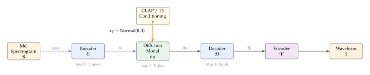
The mathematical advantage of the three-stage decomposition can be quantified through the lens of the evidence lower bound (ELBO). For a standard diffusion model operating on mel spectrograms, the variational bound decomposes as (ELBO Pixel) When the diffusion operates in the latent space of a pretrained autoencoder, we instead lower-bound in two stages: (ELBO Latent 1) where captures the reconstruction quality of the autoencoder. The key insight is that involves denoising in the low-dimensional latent space, which is computationally cheaper and statistically easier to learn.
Proposition 20 (Computational Advantage of Latent Diffusion).
Let be a mel-spectrogram and its latent encoding, with spatial compression ratio . Write and , so that . Then, for the same denoising architecture applied in the two spaces:
every convolutional layer costs a number of multiply–accumulates proportional to the number of positions it is evaluated at, so the convolutional part of the cost satisfies (Latent COST Ratio)
every global self-attention layer costs in the number of positions it attends over, so an attention layer that is moved from full resolution to latent resolution is cheaper by .
Consequently the per-step cost ratio lies between and , and equals whenever the network is convolution-dominated. The same ratio applies to total training cost when the number of diffusion steps is held fixed.
Proof.
A convolution with input channels, output channels and kernel size costs multiply–accumulates per output position, and the number of output positions at a given resolution level is proportional to the number of input values . The per-layer cost is therefore linear, not quadratic, in , and summing over layers preserves linearity, which gives (Latent COST Ratio). Self-attention over positions costs because it forms all pairwise scores, so shrinking the position count by shrinks that term by . In a U-Net the attention blocks are placed at the coarsest resolutions, where the position count is already reduced by the downsampling stack, so they contribute a small fraction of the total FLOPs and the convolutional term dominates. The overall ratio is thus a convex combination of and , dominated by .
Caution.
It is tempting to write the saving as on the grounds that “the network is quadratic in its input size”. It is not: a convolutional denoiser is linear in the number of values it processes. For the typical of audio autoencoders the honest per-step saving is therefore about , not . The figure is attainable only in the limit of a denoiser that is pure global self-attention at full resolution, which no deployed audio LDM is.
Remark 27.
The compression ratio cannot be increased without bound. As grows, the autoencoder must discard increasingly perceptually relevant information, degrading the quality ceiling of the entire pipeline. In practice, audio latent diffusion systems use , balancing compression against reconstruction fidelity. The autoencoder's reconstruction loss (measured by Fréchet Audio Distance or multi-resolution STFT loss) serves as an upper bound on the quality achievable by any diffusion model operating in that latent space, regardless of how well the diffusion model itself is trained.
Autoencoder design for audio latent diffusion.
The audio autoencoder is typically a variational autoencoder (VAE) trained on mel spectrograms. The encoder produces a mean and log-variance for each latent position: (VAE Encode) where the reparametrisation trick enables gradient-based training. The VAE is trained with a combination of reconstruction loss and KL regularisation: (VAE LOSS) where is the multi-resolution STFT loss (HiFi-GAN Training Losses) and is a small weighting coefficient (typically to ) to prevent posterior collapse while keeping the latent space smooth.
Caution.
The KL regularisation weight requires careful tuning in the audio setting. Too large a value forces the latent space toward a standard Gaussian, destroying audio structure and leading to blurry, reverberant reconstructions. Too small a value produces a latent space with “holes” (regions of low density) that confuse the diffusion model during generation. A common diagnostic is to sample from the prior and decode: if the result is completely unintelligible, the KL weight is too low; if it sounds like white noise convolved with a room impulse response, the KL weight is too high.
AudioLDM: The Foundational System
AudioLDM, introduced by Liu et al. (2023), was the first system to demonstrate that the latent diffusion paradigm from image generation could be transferred wholesale to audio, achieving state-of-the-art text-to-audio results with a remarkably simple architecture. The system consists of three components: a pretrained audio VAE, a U-Net-based diffusion model conditioned on CLAP embeddings, and a HiFi-GAN vocoder.
Architecture.
The AudioLDM pipeline instantiates Definition 33 as follows. The audio VAE is trained on mel spectrograms of size (typically , for 10-second clips at 16,kHz with a hop size of 160 samples). The encoder compresses by a factor of along the time axis and along the frequency axis, producing latents . The U-Net follows the architecture from Stable Diffusion (Rombach et al., 2022), adapted for the two-dimensional latent spectrogram shape: it uses 2D convolutions (treating time and compressed-frequency as spatial axes), self-attention at the bottleneck resolution, and cross-attention layers that attend to the conditioning embeddings.
CLAP conditioning.
The conditioning embedding is obtained from a pretrained CLAP model (CLAP: Contrastive Language–Audio Pretraining). Given a text prompt , the CLAP text encoder produces a global embedding . This embedding is injected into the U-Net via cross-attention: (Audioldm Crossattn) where represents the spatial features at a given U-Net layer and the CLAP embedding is treated as a sequence of length 1. This is equivalent to the image-domain cross-attention mechanism studied in 19, with CLAP replacing CLIP as the conditioning encoder.
Proposition 21 (AudioLDM Training Objective).
The AudioLDM diffusion model is trained to minimise the noise-prediction objective in the latent space of the pretrained audio VAE\@. Given a clean latent , a noise sample , a uniformly sampled timestep , and a conditioning embedding , the training loss is (Audioldm LOSS) where is the noised latent following the standard DDPM forward process with cumulative noise schedule .
Proof.
This follows directly from the DDPM training objective (19), applied to the latent variable instead of the data variable . The key observation is that once the autoencoder is frozen, the distribution of over the training set defines a fixed “data distribution” in latent space, and the standard diffusion framework applies without modification. The conditioning embedding enters through the cross-attention layers of and does not affect the mathematical form of the loss.
Example 15 (AudioLDM Inference).
To generate a 10-second audio clip from the text prompt “a dog barking in a park with birds singing,” AudioLDM proceeds as follows:
Encode the text prompt using CLAP: .
Sample initial noise: , with .
Run the DDPM reverse process for steps (or DDIM for 50 steps), each step applying the U-Net .
Decode the denoised latent: .
Convert to waveform using HiFi-GAN: .
The entire process takes approximately 5 seconds on an A100 GPU with DDIM, achieving a real-time factor of .
Insight.
CLAP as a universal audio conditioning interface. A subtle but important property of AudioLDM's design is that the CLAP text encoder can be replaced at inference time with the CLAP audio encoder. Since both encoders map to the same embedding space, one can condition generation on a reference audio clip instead of a text description, enabling audio-to-audio style transfer without any architectural changes. This “plug-and-play” property is a direct consequence of the symmetric training objective studied in CLAP: Contrastive Language–Audio Pretraining: the shared embedding space is agnostic to whether the input is text or audio.
AudioLDM2: Language-Aligned Latents
AudioLDM2 (Liu et al., 2024) addresses a fundamental limitation of the original AudioLDM: the CLAP embedding is a single global vector, which provides only a coarse, non-temporal conditioning signal. A text prompt like “a piano plays a gentle melody, then thunder rumbles” describes a temporal sequence of events, but a single CLAP vector cannot represent this ordering. AudioLDM2 introduces two architectural innovations to enable richer, temporally structured conditioning: an AudioMAE-based representation learning module and a Language-Oriented Audio (LOA) generation framework.
AudioMAE representation.
AudioLDM2 replaces the single CLAP vector with a sequence of latent vectors derived from an AudioMAE (Audio Masked Autoencoder). The AudioMAE is a vision transformer trained on mel spectrograms using the masked autoencoding objective: random patches of the spectrogram are masked, and the model learns to reconstruct them from the visible patches. After pretraining, the AudioMAE encoder produces a sequence of patch embeddings that capture both local spectral features and global temporal structure.
Definition 34 (AudioMAE Representation).
Let be a mel spectrogram partitioned into non-overlapping patches of size , yielding patches. The AudioMAE encoder maps the spectrogram to a sequence of patch embeddings, each of dimension . During pretraining, a fraction (typically ) of the patches are masked, and the model is trained to minimise (Audiomae LOSS) where is the set of masked patch indices, is the ground-truth patch, and is the model's reconstruction.
Language-Oriented Audio (LOA) generation.
The central innovation of AudioLDM2 is the LOA module, which bridges the gap between language representations and audio latent representations. LOA consists of a GPT-2-style autoregressive model that takes as input a sequence-level language representation (from FLAN-T5 or CLAP) and outputs a sequence of AudioMAE-compatible embeddings. These embeddings serve as the conditioning signal for the latent diffusion model, replacing the single CLAP vector of AudioLDM\@.
Formally, let be the output of the language encoder (FLAN-T5) for a text prompt, where is the sequence length and is the language embedding dimension. The LOA module generates a sequence of AudioMAE-like tokens: (LOA) where is the -th generated audio token and is the target sequence length (matching the temporal resolution of the diffusion model's conditioning input).
The generated sequence then serves as the cross-attention key and value for the latent diffusion U-Net: (Audioldm2 Crossattn) where denotes the spatial features at a given U-Net layer. Unlike AudioLDM's single-vector conditioning, this provides spatially varying conditioning: different temporal positions in the latent spectrogram attend to different audio tokens, enabling the model to generate temporally structured outputs.
Proposition 22 (Expressivity of Sequence-Level Conditioning).
Let be the attention head dimension and the number of conditioning tokens. The cross-attention output at spatial position of the U-Net is (SEQ COND Output) When (AudioLDM), for all , and the conditioning is spatially uniform: for all . When (AudioLDM2), the attention weights vary with , allowing different spatial positions to receive different conditioning signals.
Proof.
For , the softmax over a single element is trivially regardless of , so the output is , which is independent of . For , the attention weights depend on the query , which varies across spatial positions . Different queries produce different weight distributions over the conditioning tokens, yielding spatially varying outputs.
Remark 28.
AudioLDM2 is designed as a unified framework that generates speech, sound effects, and music from the same architecture by varying only the language encoder. For sound effects and music, FLAN-T5 embeddings are used; for speech synthesis, a speaker embedding from a pretrained speaker verification model is concatenated with the T5 embeddings. The LOA module learns to translate these heterogeneous conditioning signals into a common AudioMAE-like representation, enabling the same diffusion model to serve all three domains.
MusicLDM: Beat-Synchronous Augmentation
Music generation poses unique challenges compared to general audio generation. Music has strong temporal structure: beats, bars, phrases, and sections create hierarchical rhythmic patterns that listeners perceive and expect. MusicLDM (Chen et al., 2024) addresses this by introducing beat-synchronous mixup, a data augmentation strategy that creates new training examples by mixing pairs of music clips at beat boundaries. The insight is that mixing at metrically meaningful points produces musically coherent augmentations, whereas mixing at arbitrary time points produces artefacts that degrade generation quality.
Definition 35 (Beat-Synchronous Mixup).
Let and be two music clips with their corresponding text descriptions, and let and be their detected beat positions (in samples), with inter-beat intervals and seconds. A beat-synchronous mixup produces a new training pair as follows:
Tempo match. Resample by the factor so that both clips share the inter-beat interval . Write for the stretched clip and for its beat positions.
Phase align. Circularly shift by samples so that the two beat grids coincide. Write .
Mix. Draw a mixing ratio for a hyperparameter (typically ) and form the convex combination (BEAT Mixup)
Mix the conditioning. Mix the CLAP embeddings of the two captions with the same coefficient, .
MusicLDM applies exactly this construction in two places: to the waveforms, as written above, and to the VAE latents, replacing (BEAT Mixup) by after the same tempo matching and phase alignment.
Caution.
Beat-synchronous mixup is a simultaneous mix of two tempo-aligned clips, not a splice from one clip to the other at a beat. The splice variant - play up to a beat, then continue with - is a different augmentation with a different purpose (it teaches the model about transitions rather than about superposition), and it is not what MusicLDM does. The distinction matters because the two produce different artefacts: the splice risks a discontinuity at one instant, whereas the mix risks two competing pulses across the whole clip.
The key property of beat-synchronous mixup is that the two clips' pulses coincide, so the mixture is heard as one piece of music at one tempo. This contrasts with naive mixup at a random offset, which superimposes two beat grids at an arbitrary phase and is heard as two recordings playing over each other.
Proposition 23 (Beat-Synchronous Mixup Preserves a Single Pulse).
Let and be the inter-beat intervals (in seconds) of clips and , and assume both clips have approximately constant tempo. If the beat detection algorithm has error samples for all detected beats, then the mixed clip of Definition 35 has the following properties:
After tempo matching, both components have inter-beat interval to within the resampling error, so the grid offset does not accumulate over the clip.
Every beat of the stretched, shifted clip lies within samples of a beat of , since each of the two anchor beats used to compute is located to within .
The resulting misalignment is at most seconds throughout.
Proof.
For (i), resampling by maps an inter-beat interval of onto one of exactly; under the constant-tempo assumption every interval of equals , so every interval of equals and the two grids have identical spacing. Two grids of identical spacing differ by a constant offset, which is what (i) asserts. For (ii), that constant offset is evaluated on the true beat positions; since is computed from the two estimated anchors and each is within of the truth, the offset is bounded by . Part (iii) is (ii) divided by .
Remark 29.
The numbers matter here. For typical beat-tracking accuracy ( ms ) at Hz, Proposition 23 bounds the misalignment by ms, below the roughly ms at which two onsets stop fusing into one perceived attack. Mixing at a random offset instead gives a misalignment distributed uniformly on , with mean : at 120 BPM that is ms, an order of magnitude past the fusion threshold, which is precisely why unaligned mixup sounds like two songs rather than one.
Beyond the beat-synchronous construction itself, MusicLDM also considers mixing only the conditioning embeddings, , without touching the audio. This operates in the semantic space rather than the acoustic one and needs no beat tracking, which makes it the applicable variant for general sound effects, where there is no beat structure to align in the first place.
Example 16 (MusicLDM Training Data Size).
MusicLDM is trained on approximately 2,000 hours of music with text captions, a relatively modest dataset compared to the millions of hours used by commercial music generation systems. Beat-synchronous mixup effectively increases the training diversity by producing possible mixup pairs from original clips. For clips (roughly 2,000 hours at 72 seconds per clip), this yields approximately possible augmented examples, a combinatorial explosion that substantially enriches the training distribution without requiring additional data collection.
Diffusion Architectures for Audio
The previous section established the three-stage latent diffusion pipeline and studied systems built around U-Net denoisers. In this section, we examine the architectural design space more broadly. The central question is: what neural network architecture should serve as the denoising backbone for audio diffusion? Two families dominate the landscape: the U-Net, inherited from image diffusion (19), and the Diffusion Transformer (DiT), adapted from the vision transformer paradigm (Video Diffusion Transformer (DiT)). Each architecture offers distinct mathematical trade-offs in terms of inductive bias, scalability, and conditioning flexibility.
We study three influential systems that explore different points in this design space: Stable Audio, which introduces timing conditioning and, in its later releases, moves to a DiT backbone (Stable Audio: Timing Conditioning, and the Move to a DiT); Noise2Music, which uses a cascaded U-Net architecture (Noise2Music: Cascaded Generation); and Moûsai, which combines diffusion with efficient U-Net variants (Moûsai: Efficient Diffusion for Long Audio).
U-Net vs. DiT: The Architectural Divide
The U-Net and the DiT represent fundamentally different inductive biases for the denoising function .
U-Net.
The U-Net processes the latent spectrogram through an encoder-decoder structure with skip connections at matching resolutions. At each resolution level , the encoder applies a sequence of residual blocks and (optionally) self-attention: (UNET Block) where the timestep is injected via adaptive group normalisation (AdaGN), and the conditioning enters through cross-attention. The decoder mirrors this structure with upsampling operations and skip connections from the encoder. The U-Net's multi-scale structure is a natural fit for spectrograms, which exhibit different statistical properties at different time-frequency scales.
DiT.
The Diffusion Transformer treats the latent representation as a sequence of patches and processes it with a standard transformer encoder. The latent is first patchified into a sequence of tokens, each of dimension : (DIT Patchify) Each transformer block then applies self-attention and a feed-forward network with adaptive layer normalisation (adaLN) for timestep and conditioning injection: (DIT Block) where are scale and shift parameters predicted from the timestep and conditioning embeddings. The DiT's advantage is scalability: it has no resolution-specific components, and its compute scales linearly with the number of layers for a fixed sequence length, making it straightforward to scale to billions of parameters.
Proposition 24 (Receptive Field Comparison).
Consider a latent spectrogram of temporal length .
For a U-Net whose encoder has resolution levels, one convolution of kernel size (stride 1) per level, and a factor-2 downsample between levels, the bottleneck sequence length is tokens, and the receptive field of a bottleneck unit, measured back in input tokens, is (UNET RF) Within a single resolution, stacked kernel- convolutions give a receptive field of only .
For a DiT with transformer layers, every layer has global receptive field over all tokens (full self-attention). After a single layer, each token can attend to any other token.
Proof.
Receptive fields of stacked convolutions add, they do not multiply. At a fixed resolution, composing two layers with receptive fields and gives , so layers of kernel give . When a factor-2 downsample precedes level , each step at that level spans input positions, so level contributes rather than , and summing the geometric series over the levels and adding the single central position gives (UNET RF). The downsampling also reduces the temporal dimension from to at the bottleneck, so self-attention placed there is global over the compressed sequence; note that this is a sequence length, a different quantity from the receptive field. For the DiT, self-attention computes pairwise interactions between all tokens at every layer, giving a global receptive field of from the first layer onward.
Example 17 (How Far Back a U-Net Level Actually Sees).
Take and , and the Stable Audio latent rate of Hz. Stacking the six convolutions at a single resolution gives a receptive field of tokens. Inserting the factor-2 downsamples gives tokens, or seconds - enough to span a musical phrase, which is the whole point of the hierarchy. The figure that an “exponential in depth” reading would suggest is not attained by either arrangement; convolutional receptive fields grow linearly in depth at fixed resolution and only geometrically once downsampling is added.
Stable Audio: Timing Conditioning, and the Move to a DiT
Stable Audio (Evans et al., 2024) introduces two innovations that have since been widely copied: explicit timing conditioning, which enables variable-length generation up to 95 seconds, and a waveform-domain VAE that bypasses the mel-spectrogram representation entirely.
Caution.
Two distinct systems share the “Stable Audio” name and they must not be conflated. The 95-second timing-conditioned system described in this subsection performs latent diffusion with a U-Net denoiser (roughly 907M parameters) over waveform-VAE latents. The DiT denoiser, with the layer counts and widths given below, belongs to the later Stable Audio Open release, which generates shorter clips (up to about 47 seconds). The timing conditioning of Definition 36 is orthogonal to that choice: it is a way of injecting two scalars through adaptive normalisation and works equally well in either backbone. This chapter's own comparison table lists Stable Audio under “latent diffusion” rather than “DiT” for exactly this reason.
Waveform VAE.
Unlike AudioLDM, which compresses mel spectrograms, Stable Audio trains its VAE directly on raw waveforms. The encoder operates on the waveform (at 44.1,kHz) and produces a continuous latent sequence with a temporal compression factor of (from 44.1,kHz to approximately 21.5,Hz). This extreme compression is achieved through a series of strided 1D convolutions: (Stable Audio VAE) where are the stride factors of successive convolutional layers, with .
Note that is the compression of the clock, not of the data. The encoder widens as it shortens: one scalar sample per s becomes a vector of channels per s. In the units of Proposition 20, the compression ratio is a ratio of value counts, which is what governs the per-step cost, and which sits squarely in the band of Remark 27. Quoting as though it were overstates the saving by a factor of .
Definition 36 (Timing-Conditioned DiT).
A timing-conditioned DiT augments the standard DiT architecture with two additional scalar conditioning signals:
Start time : the timestamp (in seconds) at which the generated audio segment begins within the full track.
Total duration : the total duration of the track from which this segment originates.
These scalars are encoded via sinusoidal embeddings: (Timing Embed) where are learnable or fixed frequency bases, and . The timing embeddings are concatenated with the diffusion timestep embedding and projected into the adaLN parameters of each DiT block.
Insight.
Why timing conditioning matters for music. Music tracks have structure at multiple temporal scales: an intro at the beginning, a build-up toward the middle, and an outro at the end. Without timing information, a diffusion model trained on random crops of full tracks has no way to know whether it should generate an intro, a chorus, or an ending. The start-time conditioning resolves this ambiguity, allowing the model to generate structurally appropriate content for any position within a track. The duration conditioning further informs the model about the overall scale of the piece: a 30-second jingle has different structural expectations than a 5-minute song.
Architecture details of the Stable Audio Open DiT.
The DiT released with Stable Audio Open uses transformer layers with hidden dimension and 24 attention heads, for a total of approximately 1.06B parameters. (The 95-second timing-conditioned system discussed above is a U-Net of about 907M parameters; only the conditioning interface is shared.) Conditioning is provided through three channels:
Text embeddings from a CLAP text encoder, injected via cross-attention at every transformer block.
Timing embeddings , injected via adaLN alongside the diffusion timestep.
Diffusion timestep embedding , also injected via adaLN.
The combined conditioning vector for adaLN is (Stable Audio COND) from which the scale and shift parameters are extracted for each transformer layer.
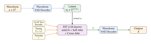
Example 18 (Stable Audio Generation Parameters).
To generate a 45-second music track with Stable Audio:
Waveform length: samples.
Latent sequence length: tokens. (Note , which exceeds the available samples; 968 tokens cover seconds, and the remaining samples form a partial frame that is padded or discarded.)
Latent channels: .
Denoiser input: a sequence of tokens, each of dimension , projected to .
Timing conditioning: (start of track), (total duration).
Diffusion steps: 100 (using DPM-Solver++).
Each forward pass processes activations through 24 layers, requiring approximately ,ms on an A100. Total generation time: seconds, well under real time.
Noise2Music: Cascaded Generation
Noise2Music (Huang et al., 2023) takes a different architectural approach: instead of a single diffusion model in latent space, it uses a cascade of two diffusion models operating at different resolutions in spectrogram space. This mirrors the cascaded approach used in image generation (e.g., DALL-E 2, Imagen) and provides a natural decomposition of the generation problem into coarse structure and fine detail.
Definition 37 (Cascaded Audio Diffusion).
A cascaded audio diffusion system consists of two stages:
A base model that generates a low-resolution mel spectrogram from text conditioning.
A super-resolution model that upsamples the base spectrogram to full resolution , conditioned on both the text and the low-resolution output.
The full generation factorises as (Cascaded Factor)
Base model.
The Noise2Music base model generates a full 30-second clip at a reduced temporal resolution; in the running example of this subsection we take frames at a ms hop, which covers seconds and keeps the arithmetic small. It uses a 1D U-Net operating along the time axis, treating the frequency bins as channels. The text conditioning is provided by a frozen T5 encoder whose embeddings are injected via cross-attention. A second large language model, LaMDA, appears elsewhere in the Noise2Music pipeline, but in a different role: it is used offline to pseudo-label unlabelled music with captions, enlarging the paired training set. It is not the conditioning encoder.
Super-resolution model.
The super-resolution model takes the base spectrogram (bilinearly upsampled to full resolution) as an additional input channel, concatenated with the noisy full-resolution spectrogram at each diffusion step: (SR Input) This concatenation-based conditioning allows the super-resolution model to use the base spectrogram as a structural guide while adding high-frequency detail.
Proposition 25 (Cascaded Generation: Error Propagation).
Let be the base model's output and be the super-resolution model's output. Define the error at each stage as where and are the ground-truth spectrograms at each resolution. If the super-resolution model has Lipschitz constant with respect to its conditioning input, then (Cascaded Error Bound) where is the error of the super-resolution model when given the ground-truth base spectrogram. Errors from the base model thus propagate multiplicatively through the cascade.
Proof.
By the triangle inequality and the Lipschitz property:
Caution.
Cascaded architectures inherit a fundamental fragility: errors in the base model are amplified by the super-resolution stage. If the base model generates spectrogram content with the wrong temporal structure (e.g., placing a drum hit at the wrong position), the super-resolution model will faithfully add fine detail to this incorrect structure, producing a high-resolution but structurally wrong output. This is why modern systems increasingly prefer single-stage latent diffusion (AudioLDM, Stable Audio) over cascades.
Moûsai: Efficient Diffusion for Long Audio
Moûsai (Schneider et al., 2023) addresses the challenge of generating long music clips (up to 48 seconds) with limited computational resources. Its key insight is that a carefully designed 1D U-Net operating on waveform-domain latents can achieve competitive quality with far fewer parameters than spectrogram-based alternatives.
Cascaded 1D U-Net.
Moûsai uses a two-stage design, but the latent space is its own, not a borrowed neural codec. The first stage is a diffusion magnitude-autoencoder: a spectrogram magnitude is compressed by a factor of roughly into a continuous 1D latent sequence, and a diffusion decoder reconstructs the waveform from it, phase included. The second stage is a latent diffusion model that generates those latents from text. Both stages use 1D temporal convolutions along the time axis.
The 1D U-Net replaces the 2D convolutions of spectrogram-based models with 1D temporal convolutions: (Mousai CONV) where are the convolution weights at level with kernel half-width , is a nonlinearity, and is the timestep-dependent scale from adaptive normalisation.
Proposition 26 (Parameter Efficiency of 1D vs. 2D U-Net).
Consider a U-Net with levels, each containing residual blocks with channel width and kernel size .
A 2D U-Net (for spectrograms) has convolutional weight tensors of shape per layer, yielding total convolution parameters.
A 1D U-Net (for waveform latents) has convolutional weight tensors of shape per layer, yielding total convolution parameters.
For typical kernel sizes ( for 2D, for 1D), the 1D U-Net uses approximately fewer convolution parameters, but the real savings come from the reduced spatial dimensions: the 1D latent sequence is typically 4 to 8 times shorter than the 2D spectrogram along its non-channel dimensions.
Proof.
The convolution parameter count follows directly from the weight tensor shapes. For a 2D convolution with input and output channels and kernel size , the weight tensor has entries. For a 1D convolution with the same channel count and kernel size , the weight tensor has entries. Summing over levels and blocks per level gives the stated scaling.
Remark 30.
Moûsai's headline claim is a compute claim: it generates up to 48 seconds of stereo music at 48,kHz from a model trained on a single A100 GPU\@. By comparison, AudioLDM generates at most 10 seconds at 16,kHz, and the Stable Audio family reaches 95-second generation at 44.1,kHz with roughly a billion parameters and substantially more training compute. The efficiency of Moûsai stems from two choices working together: a -compressed 1D latent, and a purely convolutional denoiser, which avoids the quadratic cost of self-attention over long sequences.
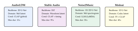
Diffusion in Audio Latent Spaces
The previous two sections described the architectures and systems that instantiate latent audio diffusion. This section examines the diffusion process itself in detail: the forward noising process that corrupts audio latents, the noise schedules that control corruption speed, and the alternative parameterisations of the denoising objective that affect training dynamics and generation quality. While the mathematical framework follows the general theory developed in 19, the audio domain introduces specific considerations related to the structure of audio latent spaces, the multi-scale nature of audio signals, and the interaction between noise schedules and perceptual quality.
The Forward Process in Audio Latent Space
Let be a clean audio latent obtained from a pretrained encoder . The forward diffusion process is a Markov chain that progressively adds Gaussian noise: (Forward) where is the noise schedule with . Using the reparametrisation trick, we can sample directly from without iterating through the chain: (Forward Closed) where is the cumulative signal retention coefficient. Equivalently, (Forward Reparam)
Definition 38 (Signal-to-Noise Ratio for Audio Latents).
The signal-to-noise ratio (SNR) at diffusion timestep for the forward process in (Forward Closed) is (SNR) The SNR decreases monotonically from (clean signal) to (pure noise). In log-space, (LOG SNR)
The SNR is the central quantity governing the diffusion process. It determines how much signal information remains at each timestep and directly controls the difficulty of the denoising task. For audio latent spaces, the choice of noise schedule (i.e., how the SNR decreases from to ) has a profound impact on generation quality.
Noise Schedules for Audio
The noise schedule (or equivalently, the function in continuous time) determines the rate at which the signal is corrupted. The general theory of noise schedules is developed in Noise Schedules for Video; here we focus on the specific considerations that arise when the diffusion process operates in an audio latent space.
Definition 39 (Common Noise Schedules).
Three noise schedules commonly used in audio diffusion:
Linear schedule (Ho et al., 2020): , where and .
Cosine schedule (Nichol and Dhariwal, 2021): (Cosine Schedule) where is a small offset to prevent from reaching exactly zero.
Sigmoid schedule: (Sigmoid Schedule) where and control the range of the log-SNR.
Proposition 27 (Cosine Schedule Preserves Information Longer).
Let be the first timestep at which the noise energy equals or exceeds the signal energy. For and the parameters of Definition 39, (Schedule Crossings) The cosine schedule therefore holds - more signal than noise - for more timesteps than the linear schedule.
Proof.
, so if and only if ; both crossings are found by locating .
For the linear schedule, with . Taking logarithms, , a quadratic in . Solving gives , and evaluating the exact product confirms and , so .
For the cosine schedule, first drop the offset: , and gives , hence . Restoring moves this only slightly. Writing , the condition has solution , i.e. , and the discrete schedule first drops below at (, ). The offset is worth steps, not .
The gap is .
Caution.
The two crossings are often quoted as and . Neither survives contact with the definitions. At the linear schedule already has , an SNR of - the noise energy is 21 times the signal energy, nowhere near parity. At the cosine schedule has , an SNR of . The qualitative claim is nonetheless right, and by a wider margin than the folklore numbers suggest: cosine really does keep more signal than noise for roughly twice as long.
Remark 31.
Audio latent spaces differ from image latent spaces in their distributional properties. Audio latents tend to have:
Higher dynamic range: loudness variations across a clip create latent dimensions with very different variances, meaning some dimensions are corrupted much faster than others under an isotropic noise schedule.
Temporal correlations: adjacent latent frames are highly correlated (music changes slowly relative to the latent frame rate), creating low-frequency structure that requires more noise to obscure than the high-frequency details.
Sparser spectra: at any given moment, only a few frequency bands are active (e.g., a single instrument playing), concentrating the signal energy in a low-dimensional subspace of the latent space.
These properties suggest that audio diffusion may benefit from noise schedules that spend more time in the high-SNR regime (preserving coarse temporal structure longer) compared to image diffusion. The cosine schedule partially addresses this, but systems like Stable Audio use custom sigmoid schedules tuned specifically for their waveform latent spaces.
Parameterisation: , , and epsilon, x0, and v
The denoising network can be trained to predict different targets, each corresponding to a different mathematical parameterisation of the reverse process. While these parameterisations are theoretically equivalent (they all define the same conditional distribution ), they differ significantly in training dynamics, gradient magnitudes, and empirical generation quality.
Definition 40 (Three Parameterisations).
Given the noisy latent , the denoising network can be trained to predict:
Noise prediction (-parameterisation): the network predicts the noise , with loss (EPS Param)
Data prediction (-parameterisation): the network predicts the clean latent , with loss (X0 Param)
Velocity prediction (-parameterisation, Salimans and Ho, 2022): define the velocity (Velocity) and train the network to predict , with loss (V Param)
The three parameterisations are related by linear transformations. Given any one prediction, the other two can be recovered: (Param Conversion 1) The pair determines and by the inverse rotation (Param Conversion Inverse) which makes the geometry explicit: with and , the map is a rotation by in the plane they span, and is the derivative of with respect to - hence the name “velocity”.
Proposition 28 (Implicit Loss Weighting).
The three parameterisations induce different implicit weightings on the denoising signal-to-noise ratio. Fix and express every loss as a weighted squared error in the same quantity, the -prediction error. Then (EPS Weight) so the -loss emphasises high-SNR (low-noise) timesteps and its weight collapses to as ; (X0 Weight) and the -parameterisation carries (V Weight) In particular exactly, so (V Sandwich) for every . The -loss therefore tracks whichever of the other two objectives is weighting that timestep more heavily - once , below it - and is never more than a factor of two away from it. That factor is attained only at the crossover and tends to at both ends of the trajectory. (Measuring instead against the -prediction error divides all three weights by , giving , and ; the sandwich (V Sandwich) is unchanged, since it is scale-invariant.)
Proof.
The -loss first. From (Param Conversion 1), at fixed the map is affine with linear part , so which is (EPS Weight), and (X0 Weight) holds by definition.
For , the essential point is that conditional on the three errors are not independent; they are deterministically locked. Write , and . Applying (Param Conversion Inverse) to the truth and to the prediction and subtracting, (Error LOCK) The first identity already gives the result: , which is (V Weight), since .
It is instructive to see where the naive expansion goes wrong. Expanding with gives The cross term does not vanish. Although and are independent, the two errors are not: by (Error LOCK) they are anti-aligned, so and the cross term contributes exactly . Reinstating it, the weight on is in agreement with (V Weight). Finally, (V Sandwich) follows from and the elementary bounds for .
Caution.
Dropping the cross term produces the claim , i.e. that the -loss weights all timesteps equally. It does not. The truncated expression equals only at ; at it is , against the true weight . What is true, and is the property actually worth having, is (V Sandwich): up to a factor of at most two, training on is the same as automatically switching to whichever of - and -prediction is better conditioned at the current noise level, with no schedule to tune. That is a genuine balance property; uniformity is not, and was never available.
Key Idea.
Why audio systems reach for the -parameterisation. Audio signals have important perceptual content at all noise levels: at high SNR, the model must capture fine timbral details (instrument identity, room acoustics); at low SNR, it must establish coarse temporal structure (rhythm, harmony, section boundaries). The -parameterisation's emphasis on high-SNR timesteps tends to produce outputs with correct fine detail but poor global structure, while the -parameterisation tends to produce outputs with good structure but blurry detail. By (V Sandwich) the -loss sits within a factor of two of the larger of the two at every timestep, so it inherits whichever one is doing useful work and never degenerates to the other's weakness - not because its weighting is flat (it is not; falls from about at to at on the linear schedule of Definition 39), but because it is the pointwise maximum of the two, up to that factor of two. Stable Audio uses -prediction; AudioLDM2, despite often being listed alongside it, trains with the standard objective.
Example 19 (Gradient Magnitudes Across Parameterisations).
Measure every objective as a weighted squared error in the -prediction, as in Proposition 28, so that the gradient magnitude with respect to a fixed prediction error scales as . At a high-SNR timestep (, ):
-loss: .
-loss: .
-loss: .
At a low-SNR timestep (, ):
-loss: .
-loss: .
-loss: .
Read the columns, not the rows. At high SNR sits on top of ( against ) and ignores ; at low SNR it sits on top of ( against ) and ignores , whose gradient has by then shrunk by a factor of and carries almost no information about . The ratio is at both of these timesteps and reaches its worst case of exactly at . This is what “balanced” means for : not a flat gradient magnitude - moves by a factor of between these two timesteps - but a gradient that is never the small one.
Training Audio Diffusion Models
The preceding sections described what audio diffusion models predict (Section Diffusion in Audio Latent Spaces) and the architectures that implement these predictions (Section Diffusion Architectures for Audio). This section addresses the equally important question of how these models are trained. Training an audio diffusion model is considerably more than minimising the squared-error loss from (EPS Param): in practice, systems employ composite losses that combine multiple objectives, face data challenges unique to the audio domain, and require careful stabilisation techniques to prevent training collapse. We develop each of these topics in turn.
Composite Training Losses
While the core diffusion objective ((Audioldm LOSS)) provides the primary training signal, high-quality audio generation systems augment it with auxiliary losses that encode perceptual and structural priors about audio.
Definition 41 (Composite Audio Diffusion Loss).
The composite audio diffusion training loss combines the diffusion denoising objective with auxiliary terms: (Composite LOSS) where:
is the denoising loss (, , or -parameterised) from Definition 40.
is the multi-resolution STFT loss, computed on the decoded audio : (Mrstft Training) where denotes a set of STFT configurations (window sizes, hop lengths), and the sum over scales captures both magnitude and log-magnitude differences (see HiFi-GAN Training Losses).
is a CLAP-based semantic alignment loss: (CLAP Training LOSS) where is the CLAP audio encoder, is the CLAP text encoder, and is the generated mel spectrogram. This loss encourages the generated audio to be semantically aligned with the conditioning text.
is an adversarial loss from a discriminator that distinguishes real from generated spectrograms, following the GAN training paradigm.
The weighting coefficients control the relative importance of each term.
Remark 32.
Not all systems use all four loss terms. AudioLDM uses only for the diffusion model (the multi-resolution STFT loss is used only for VAE training). Stable Audio adds the multi-resolution STFT loss during fine-tuning. The CLAP alignment loss is primarily used in evaluation (CLAP Score) but some recent systems incorporate it during training as a perceptual guidance signal. The adversarial loss is most common in GAN-enhanced diffusion systems such as those used in speech synthesis.
Multi-resolution STFT loss in detail.
The multi-resolution STFT loss is particularly important for audio because it operates directly in the time-frequency domain where human perception is most sensitive. By summing over multiple STFT configurations, it captures perceptual quality at different temporal and spectral resolutions.
Proposition 29 (Multi-Resolution STFT Loss Properties).
The multi-resolution STFT loss as defined in (Mrstft Training) has the following properties:
Non-negativity: , with equality if and only if for all scales .
Phase invariance: depends only on the magnitude spectrograms, not on the phase. Two signals with identical magnitude spectra but different phases will have zero loss.
Multi-scale sensitivity: For a set of (window size, hop length) pairs, the loss is sensitive to errors at temporal scale seconds and frequency resolution Hz for each . Typical choices span samples.
Proof.
Property (i) follows from the non-negativity of norms. The Frobenius norm and norm are both non-negative, with equality iff their arguments are zero matrices. Property (ii) holds because discards the phase: if , then , which is independent of . Property (iii) follows from the time-frequency uncertainty principle: a window of size provides frequency resolution and temporal resolution (where is the hop length). Different pairs therefore capture errors at different time-frequency trade-offs.
Caution.
The phase invariance of the multi-resolution STFT loss (Property (ii)) means that it cannot detect phase-related artefacts such as phasiness or comb filtering. In practice, this is mitigated by the vocoder, which predicts phase from the magnitude spectrogram. However, for waveform-domain systems (like Stable Audio) that bypass the spectrogram representation, the multi-resolution STFT loss should be complemented with a waveform-domain loss (e.g., loss on the raw waveform) to capture phase-dependent distortions.
Data Challenges in Audio Diffusion
Training audio diffusion models confronts several data challenges that do not arise (or are less severe) in image generation.
Scarcity of paired data.
The largest paired text-to-image datasets contain billions of image-caption pairs (e.g., LAION-5B). By contrast, the largest public audio-caption datasets contain at most hundreds of thousands of pairs. AudioCaps contains approximately 46,000 10-second clips with human-written captions; Clotho contains approximately 6,000 clips, each with five captions. Even with data augmentation (e.g., MusicLDM's beat-synchronous mixup from Definition 35), the total training data for audio models is orders of magnitude smaller than for image models.
Remark 33 (The Sample-Complexity Gap, and How Much of It Is Provable).
It is tempting to turn the data shortage into a theorem. The honest version is shorter than one would like.
What is classical is the rate at which an empirical measure approaches its population measure in Wasserstein distance: for i.i.d. samples from a distribution supported on a -dimensional set with , (Dudley; Fournier and Guillin). Reading this backwards, matching a target to accuracy requires (Sample Complexity) samples. Three caveats have to travel with (Sample Complexity). First, it is a statement about the empirical measure, not about a trained diffusion model: a score network with the right inductive bias can and does beat it, which is the entire reason generative models are useful. Second, it is a worst case over distributions with -dimensional support; smoothness assumptions improve the exponent. Third, here is an intrinsic dimension, which for audio latent spaces is not something this chapter has measured - estimates from the effective rank of a latent covariance are sensitive to the threshold chosen and should not be quoted to two significant figures.
What survives without any of this machinery is the comparison that motivated the discussion. The largest paired text-to-image corpora are around pairs; the largest public audio-caption corpora are around . That is a factor of in data, against latent spaces of broadly comparable dimension. Whatever the true exponent in (Sample Complexity), a factor of in buys back only a factor of in - for any of the order of tens, essentially nothing. The gap is real; the mechanism by which audio systems close it is transfer from unpaired audio and from pretrained text encoders, not statistical efficiency.
Variable audio lengths and silence.
Audio clips in training datasets have highly variable durations (from 1 second to several minutes), and many clips contain significant silence or low-energy segments. Naive training on fixed-length crops can result in a large fraction of training examples being predominantly silent, wasting model capacity on learning the distribution of silence.
Definition 42 (Energy-Based Crop Selection).
Given an audio clip and a target crop length , the energy-based crop selection procedure:
Compute frame-level energy: , where is the frame hop.
Compute a running average energy over the crop window: .
Sample the crop start position from a distribution proportional to the running energy: (Energy CROP) where controls the concentration toward high-energy regions ( recovers uniform random cropping; always selects the loudest segment).
Label noise in audio captions.
Audio captions are notoriously noisy. A clip described as “a cat meowing” may also contain background traffic, air conditioning hum, and room reverberation not mentioned in the caption. This label noise directly affects the diffusion model's ability to learn accurate text-to-audio correspondences.
Remark 34.
Several strategies mitigate caption noise:
LLM-based caption enrichment: Use a large language model to expand terse captions (e.g., “cat meowing” becomes “a domestic cat meowing repeatedly in a quiet indoor environment with faint background noise”). AudioLDM2 uses this strategy with GPT-3.5.
Audio tagging augmentation: Run a pretrained audio tagger (e.g., PANNs) to detect additional sound events, then append the detected tags to the caption.
CLAP-based filtering: Compute the CLAP score between each audio-caption pair and discard pairs with scores below a threshold, removing the most misaligned examples.
Training Stability and Loss Balancing
When training with composite losses (Definition 41), the relative magnitudes of the different loss terms can vary by several orders of magnitude, leading to training instability. The diffusion denoising loss may have typical values in , while the multi-resolution STFT loss can range from depending on the STFT configuration. Without careful balancing, one loss term dominates the gradient signal, and the model effectively ignores the others.
Definition 43 (Gradient-Based Loss Balancer).
A gradient-based loss balancer dynamically adjusts the weighting coefficients in the composite loss to equalise the gradient magnitudes of each loss term. Let be the -th loss term and its gradient with respect to the model parameters . The balanced loss is (Balancer) where are target relative weights (reflecting the desired importance of each loss term), is a small constant for numerical stability, and is the norm of the gradient of with respect to a reference layer (typically the last shared layer before the output heads). The stop-gradient is not cosmetic: the coefficients are themselves functions of , and without it, differentiating (Balancer) would produce extra terms in - second derivatives of the model - which is neither what is intended nor what any implementation computes. In practice is read off the backward pass of the previous step and treated as a constant.
Proposition 30 (Gradient Equalisation Property).
Under the balanced loss from Definition 43 (with for simplicity, and with the coefficients stop-gradiented so that ), the effective gradient contribution of each loss term satisfies (GRAD Equal) for all . Therefore, if all target weights are equal (), the gradient contributions have equal magnitude regardless of the absolute scale of each loss.
Proof.
Direct computation: .
Remark 35.
The gradient-based loss balancer was popularised by the EnCodec system (Défossez et al., 2023), where it is used to balance the reconstruction loss, VQ commitment loss, and adversarial discriminator losses during neural codec training. The same technique transfers directly to audio diffusion training when composite losses are employed. The balancer operates with exponential moving averages of gradient norms to prevent oscillatory behaviour: (Balancer EMA) where is the EMA coefficient and indexes the training step. The smoothed estimates replace in (Balancer).
Learning rate warmup and scheduling.
Audio diffusion models are sensitive to the learning rate schedule, particularly during the early stages of training when the model's predictions are far from the target distribution. A common recipe is:
Linear warmup over the first 1,000 to 5,000 steps, ramping the learning rate from to .
Cosine decay from to over the remaining training steps.
EMA of model weights: maintain an exponential moving average of the model parameters with decay rate , and use the EMA weights for evaluation and inference.
The EMA weights produce smoother, higher-quality outputs than the raw training weights, particularly for music generation where subtle timbral consistency is important.
The Complete Training Algorithm
We now consolidate the components from the preceding subsections into a complete training algorithm for latent audio diffusion.
Algorithm 4 (Latent Audio Diffusion Training).
Input: Training dataset of audio-caption pairs; pretrained and frozen audio VAE ; pretrained and frozen text encoder ; noise schedule ; learning rate schedule ; EMA decay ; loss balancer weights ; parameterisation choice . Output: Trained denoiser (EMA weights ).
Initialise: Randomly initialise ; set ; set step counter .
repeat (until convergence or budget exhausted): enumerate[label=., leftmargin=1.5em]
Sample a mini-batch from .
Encode audio: For each , compute , where is the mel spectrogram of (or for waveform VAEs).
Encode text: For each , compute conditioning embedding . With probability (typically ), replace with the null embedding for classifier-free guidance training.
Sample noise and timestep: For each , sample and .
Construct noisy latent: .
Compute denoising prediction: .
Compute target: Based on : itemize
If : .
If : .
If : . itemize
Compute diffusion loss: .
Compute auxiliary losses: , , etc., if applicable (requires decoding at selected training steps).
Balance and combine: Apply the gradient balancer (Definition 43) to obtain .
Update parameters: .
Update EMA: .
Increment: . enumerate
Return .
Remark 36.
Several practical considerations supplement the formal algorithm:
Mixed precision: The U-Net or DiT is typically trained in bf16 (brain floating point) precision, with the loss computation and optimiser states in fp32. This halves the memory footprint and accelerates training by approximately on modern GPUs.
Gradient accumulation: For large batch sizes () that exceed GPU memory, gradients are accumulated over micro-batches before each optimiser step.
Distributed training: Audio diffusion models are typically trained across 8 to 64 GPUs using distributed data parallelism (DDP), with all-reduce for gradient synchronisation.
Validation metrics: Fréchet Audio Distance (FAD), CLAP score, and Inception Score are computed on a held-out set every 5,000 to 10,000 steps to monitor training progress.
Example 20 (Training Budget Estimation).
Consider training an AudioLDM-scale model (approximately 400M parameters) on 10,000 hours of audio with captions.
Data: 10,000 hours at 10-second crops yields training examples per epoch.
Batch size: (accumulated over 8 GPUs with micro-batch size 32).
Steps per epoch: steps.
Training duration: 200 epochs steps.
Time per step: Approximately 0.3 seconds on 8A100 (including forward, backward, and all-reduce).
Total wall-clock time: hours days.
GPU hours: A100-hours.
This is roughly cheaper than training a comparable image diffusion model (e.g., Stable Diffusion required approximately 200,000 A100-hours), reflecting both the smaller dataset size and the lower-dimensional latent space.
Remark 37 (Does Latent Diffusion Converge Faster?).
The budget above is a wall-clock statement, and it is worth being precise about what part of it is a convergence claim and what part is not.
The solid part is per-step cost. By Proposition 20, a denoiser run on a latent of values instead of a spectrogram of values costs a factor of about less per step. At that is where the order-of-magnitude saving in the estimate above comes from, and it holds step for step regardless of how either model is converging.
The tempting but unavailable part is a claim of the form (Convergence Bound) for the expected denoising errors after steps. The obstruction is not that the inequality is hard to prove; it is that the left side is not a well-defined number. The two errors are measured in different spaces, in different units, under different normalisations: rescaling the VAE's latent by a constant - which changes nothing about the model or its samples, since the decoder rescales by - multiplies by and the ratio with it. Any bound on that ratio is therefore a statement about a normalisation convention, not about convergence. The heuristic for SGD on a -dimensional quadratic does not repair this, because it too is stated in the metric of the space it is applied in.
What can honestly be compared across the two designs is the end of the pipeline: sample quality at fixed wall-clock, measured by a metric defined on decoded audio (FAD, or a listening test). On that yardstick latent diffusion does win, and the mechanism is the per-step cost above together with the easier target distribution, not a faster per-step convergence rate.
Classifier-Free Guidance for Audio
Classifier-free guidance (CFG), first introduced in image diffusion and studied in Classifier-Free Guidance for Audio, is essential for high-quality audio generation. Here we examine the specific training and inference considerations for CFG in the audio setting.
During training, the conditioning embedding is replaced with a null embedding with probability . This trains the model to produce both conditional and unconditional outputs. At inference, the guided prediction is (CFG Inference) where is the guidance scale.
Proposition 31 (CFG as Implicit Score Sharpening).
The classifier-free guided prediction in (CFG Inference) corresponds to sampling from a sharpened conditional distribution. Specifically, under the -parameterisation, the guided score function is (CFG Score) which corresponds to the score of the distribution . For , this distribution is more concentrated around the conditional modes than itself, effectively sharpening the conditional distribution and producing outputs that are more strongly aligned with the conditioning text.
Proof.
Taking the gradient of : This matches (CFG Score), confirming the correspondence. The sharpening effect follows because the likelihood ratio is highest in regions where the conditioning is most informative, and raising this ratio to the power amplifies these peaks.
Remark 38.
Text-to-audio systems as a class operate at , below the image-generation regime, for the reasons set out in Classifier-Free Guidance for Audio. Within that band the optimal scale varies by task, and the ordering runs with how much intrinsic structure the output already has: the more the signal constrains itself, the less extrapolation it tolerates before the constraint starts to break.
Speech: , the lowest of the three. Speech has strong intrinsic structure (phonemes, prosody, a speaker identity that must stay fixed), and excessive guidance produces robotic, over-articulated outputs.
Sound effects: . A caption such as “a door slamming shut” names the event almost completely, and the event itself is short enough that over-guidance has little time to accumulate audible artefacts.
Music: , the highest of the three, but also the range where over-guidance is easiest to hear: pushed past the top of it, outputs become “over-saturated” in the audio sense - compressed dynamics, exaggerated genre markers, repeated phrases - the analogue of the over-saturated images produced by high-CFG image models.
Resist the temptation to derive this ordering from caption vagueness. As Classifier-Free Guidance for Audio sets out, the observation that audio captions are vaguer than image prompts is correct but does not fix the direction of the effect: vagueness can be read as leaving room for valid variation (argue for less guidance) or as under-determining the target (argue for more), and both readings appear in the literature. What is safe is the intrinsic-structure ordering above, and the empirical fact that audio degrades audibly at lower guidance strengths than images degrade visibly.
Two further cautions when comparing these numbers with published defaults. Conventions differ - many tools expose a single scale , and (CFG Inference) makes , so a tool advertising is running ; see the warning in Classifier-Free Guidance for Audio. And the useful range depends on the noise schedule and on the conditioning-dropout rate used during training, so these bands are starting points for a sweep, not constants. The standard diagnostic remains to listen to outputs at several scales and pick the one that balances text adherence against naturalness.
Historical Note.
The application of latent diffusion to audio followed the image domain by approximately one year. Stable Diffusion (Rombach et al., 2022) demonstrated latent diffusion for images in late 2022; AudioLDM (Liu et al., 2023) applied the same framework to audio in early 2023. This timeline reflects a recurring pattern in generative modelling: techniques are first developed for images (which benefit from large datasets and well-understood evaluation metrics), then adapted to audio (where data is scarcer but the mathematical framework transfers directly). The adaptation is not merely engineering: audio-specific innovations such as beat-synchronous mixup (MusicLDM), timing conditioning (Stable Audio), and the LOA framework (AudioLDM2) demonstrate that the audio domain demands its own theoretical contributions.
Exercises
Exercise 11 (Latent Compression and Generation Quality).
Consider an audio VAE with encoder and compression ratio .
For a 10-second audio clip at 16,kHz with mel-spectrogram parameters , , compute the latent dimensionality for compression ratios . Assuming in all cases, what is for each? At which of these ratios is the entire compression coming from the channel axis, with no temporal downsampling at all? What would be at , and why should that answer make you suspicious of the fixed- assumption rather than of the arithmetic?
The VAE reconstruction error (measured by multi-resolution STFT loss) increases approximately as for constants . If the error doubles when going from to , compute . What reconstruction error would you predict at ?
Argue that the optimal compression ratio balances two competing effects: (i) the diffusion model's sample quality improves as increases (easier denoising problem), and (ii) the autoencoder's reconstruction quality degrades as increases. Sketch a qualitative plot of total generation quality (e.g., FAD) as a function of , and argue that a minimum exists.
(Challenging.) Let denote the conditional entropy of the waveform given the latent code. Show that the total information loss of the three-stage pipeline is bounded by where each term corresponds to the information lost at one stage of the pipeline. Which terms depend on the compression ratio?
Exercise 12 (Noise Schedule Design for Audio).
Consider the cosine noise schedule from (Cosine Schedule) with offset and discrete steps.
Compute for and the corresponding values. At which timestep is (equal signal and noise energy)?
Now consider the linear schedule with and . Compute for the same timesteps. Compare the rate of information destruction between the two schedules.
Design a “music-optimised” noise schedule that spends of the timesteps in the range (preserving global structure) and in the range (refining details). Express your schedule as a function and verify that it satisfies the boundary conditions and .
(Research direction.) Propose a method for learning the noise schedule from data, by treating as a parameterised function and optimising it jointly with the denoising network. What objective should be used? What constraints must the parameterisation satisfy to ensure a valid noise schedule?
Exercise 13 (Parameterisation Equivalence and Loss Weighting).
Let with .
Starting from the -prediction loss , derive the equivalent -prediction loss with its implicit SNR weighting. Show that .
Show that the -parameterisation target can be written as , and verify that . Conclude that if then is independent of , and explain why this is a statement about the target, not about the loss weighting. (A common slip writes the identity without the coefficients and ; check numerically at with , that the correct value is and the uncoefficiented one gives .)
Consider a “SNR-balanced” parameterisation with loss . Show that , and hence that and are not equal up to a constant. For which values of do the two weights agree? Sketch both weights on a log-SNR axis and describe how the two objectives allocate effort differently at the ends of the trajectory.
For a 1-dimensional latent () and the linear schedule, numerically compute and plot the loss weighting functions , , and of Proposition 28 for , all expressed as weights on the -prediction error. Verify numerically that at every , that the ratio stays in , and that it attains exactly where - which, for this schedule, is .
Exercise 14 (Cascaded vs. Single-Stage Audio Diffusion).
Consider a cascaded system (Noise2Music-style) with a base model and a super-resolution model , and a single-stage latent system (AudioLDM-style) with model .
The base model generates a mel spectrogram and the SR model upsamples to . Both use diffusion steps. If both models have the same architecture (same number of parameters), but the base model operates on fewer spatial dimensions, estimate the ratio of total inference FLOPs for the cascaded system vs. a single AudioLDM model operating on latent space.
Using the error propagation bound from Proposition 25, suppose the base model achieves and the SR model has Lipschitz constant with ideal SR error . Compute the total cascaded error. How does this compare to a hypothetical single-stage error of ?
Argue that the cascaded approach has an advantage for controllability: one can swap the base model (changing the coarse structure) while keeping the SR model fixed. Give a concrete example of how this modularity could be exploited in a music generation application.
Flow Matching for Music Generation
The diffusion models studied in the preceding sections learn to reverse a stochastic noising process: training teaches a network to predict the noise added at each timestep, and generation proceeds by iteratively denoising a sample drawn from pure Gaussian noise. While this framework has produced remarkable audio and music generation systems, it carries an inherent inefficiency. The stochastic trajectories connecting noise to data are highly curved in the latent space, requiring many small denoising steps for accurate traversal. Flow matching, introduced in 18 and connected to optimal transport in 14, offers a compelling alternative: learn a deterministic velocity field that transports noise to data along straighter paths, enabling fewer integration steps and simpler training objectives.
In this section we develop the theory and practice of flow matching for audio and music generation. We begin by recalling the essential ideas from continuous normalising flows and explaining why straighter paths translate directly to faster audio synthesis (From Diffusion to Flow Matching). We then examine two influential systems: MusicFlow, which cascades flow matching models from text to semantic to acoustic tokens (MusicFlow: Cascaded Flow Matching), and MelodyFlow, which adds melody conditioning in a non-autoregressive framework (MelodyFlow: Melody-Conditioned Flow Matching). Finally, we study optimal transport paths tailored to audio latent spaces and the reflow procedure that further straightens learned trajectories (Optimal Transport Paths for Audio).
From Diffusion to Flow Matching
Recall from 18 that a continuous normalising flow (CNF) defines a time-dependent velocity field whose integral curves transport a source distribution to a target distribution . Given an initial point , the generated sample is (CNF ODE) where follows the ODE . In audio generation, is a standard Gaussian over the latent space of an audio codec or spectrogram encoder, and is the distribution of clean audio latents.
The flow matching training objective avoids the expensive simulation required by maximum-likelihood training of CNFs. Instead, it constructs conditional probability paths that interpolate between the source and target, and trains to match the conditional velocity field of these paths. The simplest choice is the linear interpolation path: (Linear Interp) whose conditional velocity field is simply the displacement , independent of .
Key Idea.
Straighter paths, fewer steps, simpler training. The fundamental advantage of flow matching over diffusion is geometric. Diffusion models follow curved stochastic trajectories because the forward process adds noise incrementally and the reverse process must undo each increment. Flow matching constructs deterministic paths that can be made nearly straight, so that a first-order ODE solver (Euler method) with very few steps approximates the integral in (CNF ODE) accurately. For audio generation, where real-time synthesis demands fast inference, this translates directly to practical speedups.
Remark 39.
Flow matching and diffusion are not entirely distinct frameworks. As shown in 18, the probability flow ODE of a diffusion model defines a deterministic velocity field, and flow matching can be viewed as training this field directly. The key difference is in the choice of paths: diffusion models inherit their paths from the forward noising process (typically variance-preserving or variance-exploding schedules), while flow matching allows the practitioner to choose paths that are geometrically simpler, such as linear interpolations or optimal transport maps.
To make the comparison concrete, consider the number of function evaluations (NFE) needed to generate a 10-second audio clip at acceptable quality. A typical diffusion model requires 50 to 200 NFE with a DDPM-style sampler, or 20 to 50 NFE with an accelerated sampler such as DPM-Solver. A flow matching model with near-linear trajectories can achieve comparable quality with 5 to 20 NFE, representing a 5 to 10 speedup in wall-clock generation time.
Example 21 (NFE comparison for audio generation).
Consider generating 10 seconds of 24,kHz audio using a latent model with temporal compression factor 320 (i.e., 750 latent frames). Each function evaluation requires a forward pass of a transformer with 400M parameters. At half-precision on an A100 GPU, each forward pass takes approximately 15,ms.
table
Wall-clock generation time for 10,s of audio at various NFE counts.
Method NFE Time (s) RTF DDPM 200 3.00 0.30 DPM-Solver++ 30 0.45 0.045 Flow matching 10 0.15 0.015 Rectified flow 5 0.075 0.0075
Gaussian-to-data paths and the audio latent geometry.
Audio latent spaces exhibit structure that is atypical of natural image latent spaces: strong temporal correlations (adjacent latent frames encode overlapping waveform windows), a near-periodic substructure induced by musical rhythm, and highly non-isotropic marginals arising from the varying energy distribution across frequency bands. These properties have two consequences for flow matching. First, the linear interpolation (Linear Interp) may not be the most efficient path, because the intermediate points for may lie far from the data manifold. Second, the velocity field learned by the flow model inherits the temporal structure of the audio, so transformer architectures with causal or windowed attention along the time axis are natural choices for parameterising .
Definition 44 (Gaussian-preserving interpolation for audio).
A Gaussian-preserving interpolation between and with mean and covariance defines the path (Gauss Interp) so that at each time . This path preserves the Gaussian family of distributions along the trajectory, which can be beneficial when the data distribution is approximately Gaussian in the latent space (as is often the case for well-trained variational autoencoders).
MusicFlow: Cascaded Flow Matching
MusicFlow applies the flow matching framework to music generation through a cascaded architecture that mirrors the semantic-to-acoustic pipeline of earlier diffusion-based systems, but replaces the diffusion backbone with conditional flow matching at each stage. The cascade consists of two stages:
Text Semantic. A flow matching model maps Gaussian noise to semantic token embeddings, conditioned on a text embedding obtained from a pretrained language model (e.g., T5 or CLAP).
Semantic Acoustic. A second flow matching model maps Gaussian noise to acoustic latents (e.g., EnCodec or DAC embeddings), conditioned on the semantic tokens generated in stage (i).
Definition 45 (Audio Flow Matching Objective).
Let be a noise sample, let be a clean audio latent, and let denote the conditioning signal (text embedding, semantic tokens, or both). Define the interpolant for . The audio flow matching objective is (FM LOSS) The target is the constant velocity of the linear interpolation path from to .
Remark 40.
Comparing (FM LOSS) with the standard -prediction objective of diffusion models, , we note two key differences. First, the flow matching target is a displacement rather than a noise sample; conceptually, the network predicts “where to go” rather than “what noise was added”. Second, the flow matching objective does not require specifying a noise schedule (); the interpolation path is explicit and fixed. This simplifies hyperparameter tuning and removes a common source of instability in audio diffusion training.
The two stages of MusicFlow are trained independently using (FM LOSS) with different conditioning signals. At inference, text is first encoded by the language model, then passed through the semantic flow model to produce semantic tokens, which in turn condition the acoustic flow model. Both stages use an Euler ODE solver with a small number of steps (typically 10 to 25).
Optimal transport conditional paths.
The linear interpolation in (Linear Interp) pairs each noise sample with a data sample uniformly at random. This independent coupling can produce crossing paths: two distinct pairs and may have trajectories and that intersect, forcing the velocity field to be multi-valued at the intersection point. Such crossings increase the curvature of the learned velocity field and necessitate more integration steps.
MusicFlow mitigates this by using optimal transport (OT) conditional paths, as described in 14. Within each training minibatch of size , the noise samples and data samples are paired by solving a discrete optimal transport problem: (OT Coupling) where denotes the set of permutation matrices (or, more generally, doubly stochastic matrices). The OT-paired paths are less likely to cross, yielding a smoother velocity field that can be integrated with fewer steps.
Proposition 32 (OT pairing straightens the sampling trajectories).
For a velocity field , define the path curvature as the expected acceleration along a sampling trajectory, (OT Curvature Bound) where solves from . Then if and only if every sampling trajectory is a straight line traversed at constant speed, in which case the one-step Euler approximation is exact.
For Gaussian source and data, and with , the OT-paired marginal velocity field satisfies , while the independently paired marginal field satisfies for every non-degenerate pair - including , . Both fields transport to , and in the diagonal case they reach the same endpoints; what OT pairing buys is the route, not the destination.
Proof.
Characterisation of . Along a trajectory, , so forces almost everywhere: the velocity seen by the sample is constant, hence with . The converse is immediate.
Gaussian case, OT pairing. By Brenier's theorem (see 14) the quadratic-cost OT map between and is the affine map . Write , which is positive definite for every because . The conditional path is . For each fixed the map is an invertible affine bijection, so distinct trajectories never meet: the posterior is a point mass, and the marginal field coincides with the conditional one, (OT Gauss Field) Substituting gives , hence which does not depend on . Therefore identically and , for every .
Gaussian case, independent pairing. Take , , . With the pair is jointly Gaussian, so the marginal field is linear, with The acceleration along a trajectory is . Vanishing identically would require , whose only solutions are , which never vanish; but has a zero at . Hence and . (At , for instance, at .) The same argument applies coordinatewise in the diagonal multivariate case.
Caution.
Do not read the curvature off at a frozen point. It is tempting to differentiate (OT Gauss Field) in holding fixed and conclude that the OT paths are straight only when . That partial derivative is genuinely non-zero: for , and the fixed point , one computes at , and it is non-zero at every . What is zero is the total derivative along the trajectory: the convective term cancels exactly. Only the total derivative measures how curved the sampled path is, and only it controls the Euler discretisation error.
Remark 41.
Outside the Gaussian case there is no theorem asserting for arbitrary data distributions; the marginal field induced by a minibatch OT coupling is not the field of the population OT map, and minibatch OT is itself a biased estimator of the population coupling. The heuristic is nevertheless clear and is what practice observes: independent pairing makes the trajectories of different pairs cross, the posterior then changes rapidly near a crossing, and averaging over it produces a field whose direction turns sharply in time. OT pairing suppresses the crossings, and the reflow procedure of Optimal Transport Paths for Audio converts that heuristic into a quantitative and provable statement.
MelodyFlow: Melody-Conditioned Flow Matching
While MusicFlow demonstrates the viability of flow matching for text-to-music generation, many creative applications require finer control over the generated output. MelodyFlow extends the flow matching paradigm to accept melody conditioning: a reference pitch contour or hummed melody that guides the harmonic content of the generated music, while text controls higher-level attributes such as genre, instrumentation, and mood.
A distinguishing feature of MelodyFlow is its non-autoregressive architecture. Unlike the autoregressive token-based systems studied in earlier sections, MelodyFlow generates the entire audio segment in parallel by solving the ODE (CNF ODE) from to . This parallel generation naturally accommodates global conditioning signals (such as a melody contour spanning the full duration) without the left-to-right bottleneck of autoregressive models.
Conditioning mechanism.
The melody conditioning signal is a time-frequency representation of the reference melody, typically a chromagram or a pitch-class profile extracted by a pretrained pitch tracker. This is combined with the text embedding through cross-attention layers in the flow model's transformer backbone: (Melodyflow Attention) where is the hidden state at layer of the transformer. The two cross-attention modules operate independently, allowing the model to attend to text and melody information at different spatial and temporal scales.
Classifier-free guidance with dual conditions.
When both text and melody conditions are present, MelodyFlow applies a two-scale classifier-free guidance scheme. During training, the text condition is dropped independently with probability and the melody condition with probability . At inference, the guided velocity combines three predictions: (DUAL CFG) where and are separate guidance scales. Setting recovers text-only generation. Setting with removes the guidance on the text condition, but not the text itself: both evaluations in the melody term, and , still receive , so the text prompt continues to shape the output. Melody-only generation requires dropping from the conditioning arguments as well, that is, replacing the melody term by .
Remark 42 (Where a sample-efficiency advantage could come from).
It is often asserted that flow matching is more sample-efficient than diffusion. It is worth being precise about what such a claim could mean, because the two objectives regress onto different targets and their errors are therefore not directly comparable.
Write the excess risk of a learned field as the usual sum of a statistical term (how well the empirical minimiser approximates the population minimiser within the function class) and an approximation term (how well the function class represents the population target). Flow matching and -prediction, trained on the same architecture and the same clips, face the same statistical term: both are least-squares regressions of a bounded target on the same inputs, so nothing distinguishes them there.
Any advantage must therefore live in the approximation term, and this is where the choice of coupling enters. Under independent coupling the regression target turns sharply with wherever conditional paths cross; under OT or reflow coupling it turns much less, and in the Gaussian case of Proposition 32 it does not turn at all. A target that varies less is easier for a fixed-capacity network to fit. This is a statement about the target, not a rate: we know of no bound that converts a curvature reduction into a quantified sample-complexity gain for realistic audio distributions, and any such bound would have to account for the fact that minibatch OT is a biased estimator of the population coupling. The honest summary is that flow matching with straightened paths buys inference steps, provably (Theorem 2), and buys training samples only heuristically.
Optimal Transport Paths for Audio
The OT pairing described in MusicFlow: Cascaded Flow Matching operates within minibatches and provides only an approximation to the true optimal transport map between the noise and data distributions. In this subsection, we develop the theory of rectified flows for audio, which iteratively straighten the learned trajectories toward the true OT map, achieving near-linear paths that can be traversed in very few steps.
The key insight, due to Liu et al. (2023), is that the reflow procedure takes a trained flow model and uses its own generated trajectories as training data for a new model, whose paths are provably straighter.
Definition 46 (Reflow procedure for audio).
Let denote the velocity field after rounds of reflow. The procedure is:
Initialise: Train using the flow matching objective (FM LOSS) with independent coupling.
Generate pairs: For each noise sample , solve the ODE from to to obtain .
Retrain: Train using the flow matching objective with the deterministic coupling .
Repeat steps (2)–(3).
Theorem 2 (Rectified flow: straightening and its rate).
Let denote the population-optimal velocity field at reflow iteration , i.e., the minimiser of over all measurable functions, where is the ODE endpoint produced by the previous iterate and . Define the straightness deficit of a coupling with marginal field as (Straightness) Then:
One-round improvement. (Reflow Descent) In particular the transport cost is non-increasing, and it strictly decreases by exactly the amount of straightness still missing.
Rate. Summing (Reflow Descent) over telescopes, so for every (Reflow RATE)
What straightness buys. if and only if every trajectory of is a straight line traversed at constant speed, in which case the single Euler step reproduces exactly.
Proof.
Throughout, write for the endpoint coupling at round , for the interpolant (a straight line by construction), and for the marginal field fitted to that coupling. Because is a conditional expectation, , the orthogonality of the least-squares residual gives, for every , (Reflow Pythagoras) Integrating over turns the last term into , the straightness deficit of the coupling that was fitted to.
Part (i). Let solve from , so that . A standard property of the marginal field (18) is that it reproduces the marginals of the interpolant: for every . By Jensen's inequality applied to , the last equality because the two processes share their time- marginals. Combining with the integrated form of (Reflow Pythagoras) yields (Reflow Descent).
Part (ii). Since , (Reflow Descent) shows the sequence is non-increasing and non-negative, and . Summing over telescopes to , and dividing by gives (Reflow RATE).
Part (iii). forces for almost every , i.e., the field agrees with the chord at every point of the interpolant. The interpolant then solves the ODE, so the sampled trajectory is the straight line, its speed is constant, and . Conversely, a constant-speed straight trajectory has throughout, so .
Caution.
The straightness functional must not be defined through the ODE endpoint. A tempting but empty definition is with taken to be the endpoint of the trajectory starting at . By the ODE itself, identically, so for every velocity field, straight or not, and every claim made about it is vacuous. (Evaluated on real reflow rounds it returns floating-point zero, of order , at every .) The content of (Straightness) comes from comparing the instantaneous velocity against the chord pointwise in , which is exactly what the integral outside the expectation achieves.
Two further diagnostics are useful in practice because they are directly interpretable and cheap to measure:
the normalised chord deviation , which reports how far the trajectory bows away from its own chord as a fraction of the chord length; and
the one-Euler-step error , which is the quantity a one-step sampler actually pays.
Both vanish exactly when , and unlike they are reported in units a practitioner can budget against.
Example 22 (How many reflow iterations are worth running?).
Theorem 2 guarantees only an decay of the best straightness deficit among the first rounds; it says nothing about how the decay is distributed across rounds. Empirically the distribution is extremely lopsided: the first reflow does almost all of the work.
Running the procedure of Definition 46 on a controlled low-dimensional coupling - one where the marginal field can be computed to numerical precision, so that the measurement is not confounded by training error - the pattern is consistent. At the trajectories bow noticeably away from their chords and a one-step sampler is off by tens of percent of the chord length, so reaching a two-percent endpoint budget takes on the order of Euler steps. After a single reflow the chord deviation and the one-step error both fall by roughly an order of magnitude, and the same budget is met in about steps. A second reflow changes both diagnostics by a few percent relative and does not change the step count at all: , not . The transport cost decreases monotonically across rounds, exactly as (Reflow Descent) requires, but by ever smaller amounts.
The practical reading is the one the warning below already gives on cost grounds, and the two agree: budget for one reflow. A second reflow doubles the synthetic-data generation and retraining bill to buy a change that is not visible in the step count, and the residual error after is dominated not by path curvature but by the accuracy with which the network fits the marginal field. Reported step counts of “ after one reflow” generally reflect a straightening bottleneck that has already moved from geometry to approximation error.
Caution.
Reflow is computationally expensive for audio. Each reflow iteration requires generating a complete synthetic dataset by solving the ODE for every training sample. For a dataset of one million 10-second audio clips at 24,kHz, with 20 ODE steps per sample and 15,ms per step, the generation phase alone takes approximately on a single A100. Parallelising across 64 GPUs reduces this to roughly 1.3 hours, but the subsequent retraining phase adds another full training run. Two reflow iterations thus approximately triple the total training budget. For most practical audio systems, a single reflow combined with minibatch OT pairing during initial training provides the best cost–quality trade-off.
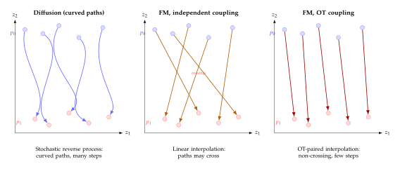
Acceleration: Consistency and Distillation
Flow matching reduces the number of ODE steps needed for audio generation from dozens to a handful. But even 5 or 10 neural network forward passes may be too many for applications that demand true real-time performance: live music accompaniment, interactive sound design, streaming text-to-speech, or in-game audio synthesis. These applications require generating audio faster than it is consumed, with latency measured in milliseconds rather than seconds.
In this section we study two families of techniques that push audio generation toward the single-step regime: consistency models, which learn to map any point along a diffusion or flow trajectory directly to the trajectory's endpoint, and progressive distillation, which iteratively halves the number of required steps by training a student model to match a teacher's two-step output in a single step.
The Real-Time Imperative
Definition 47 (Real-Time Factor).
The real-time factor (RTF) of an audio generation system is the ratio (RTF) where is the wall-clock time to generate the audio and is the duration of the generated audio. A system with generates audio faster than real time; is the real-time boundary.
For non-interactive applications (e.g., generating a soundtrack for a video), RTF is desirable but not strictly required. For interactive applications, the constraint is more nuanced: the system must produce the next chunk of audio before the current chunk finishes playing. If the chunk size is samples at sample rate , the maximum allowable latency per chunk is . For a chunk of 1024 samples at 24,kHz, this is approximately 43,ms.
Key Idea.
Audio has stricter real-time requirements than video. A dropped video frame (at 30 fps, a 33,ms gap) is barely noticeable; a 33,ms gap in audio produces an audible click or stutter that is immediately perceived as an artefact. Human auditory temporal resolution is approximately 2,ms, roughly 15 times finer than visual temporal resolution. Consequently, audio generation systems must sustain consistent low-latency output with much tighter jitter budgets than their video counterparts.
Remark 43.
RTF is hardware-dependent: a model with RTF on an A100 GPU may have RTF on a consumer laptop GPU. When reporting RTF, it is essential to specify the hardware, batch size, and numerical precision. For deployment on edge devices (phones, embedded systems), even models that are “real-time” on server hardware may fail to meet the RTF threshold, making the acceleration techniques in this section practically necessary.
Decomposing generation latency.
The total generation time for an audio diffusion or flow model can be decomposed as (Latency Decomp) where is the number of denoising or ODE steps, is the time for a single forward pass of the backbone network, is the time to compute conditioning embeddings (text encoder, CLAP, etc.), and is the time for the audio codec decoder. The acceleration techniques in this section target ; complementary approaches (model pruning, quantisation, efficient attention) target . In practice, the product dominates, so reducing from 50 to 1 yields a near-50 end-to-end speedup.
AudioLCM: Consistency Distillation for Audio
Caution.
Time runs the other way in this section. Flow Matching for Music Generation used the flow matching convention, in which is an interpolation parameter: is noise, is data, and the sampler integrates from to . Consistency models are stated in the diffusion convention, in which is a noise level on : small means clean, large means noisy, and the sampler runs from down to . To keep the two apart, this section and the two that follow it never write ; the clean audio latent is (or, where a subscript is already in use, as before) and the near-clean endpoint of a diffusion trajectory is . Only the symbol is ambiguous between the two conventions, so banning it is enough.
Consistency models, introduced by Song et al. (2023), learn a function that maps any point along the probability flow ODE trajectory to that trajectory's clean endpoint . The defining property is self-consistency: for any two points and on the same trajectory, . AudioLCM adapts this framework to latent audio diffusion models, achieving dramatic speedups.
Definition 48 (Audio Consistency Function).
Let be the probability flow ODE trajectory of a pretrained audio diffusion model, where (clean audio latent) and (noise). An audio consistency function is a neural network satisfying:
Boundary condition: for all .
Self-consistency: for all and all on the same ODE trajectory.
The boundary condition (i) ensures that the function acts as the identity near , while self-consistency (ii) ensures that applying at any timestep yields the same clean output. In practice, is parameterised using the pretrained diffusion model's architecture with a skip connection that enforces the boundary condition: (Consistency Param) where , , and is the base network.
Consistency distillation training.
The consistency function is trained by distilling the pretrained diffusion (teacher) model. Given a pair of timesteps and a noisy sample , the teacher model performs one ODE step to estimate . The consistency distillation loss then enforces self-consistency: (CD LOSS) where is a distance metric (typically the LPIPS perceptual distance adapted for spectrograms, or a combination of and -spectrogram losses), is the teacher's one-step estimate, and denotes the exponential moving average (EMA) of the student's parameters (the “target network”, updated as ).
Proposition 33 (Cost accounting for consistency distillation).
Fix a quality threshold (say FAD ). Let the teacher reach it in ODE steps and the distilled student in steps, and let be the number of network evaluations each performs per step, which is when classifier-free guidance is evaluated explicitly (one conditional and one unconditional pass) and when guidance is distilled into the weights. Then the wall-clock speedup is the ratio of network evaluations, not of steps: (Audiolcm Speedup) Consistency distillation acts on , driving it to or ; guidance distillation acts on , driving it from to . The two are independent and multiply.
Proof.
Each ODE step costs sequential forward passes of the same network, and all forward passes have equal cost, so total latency is proportional to ; the ratio follows. That can be as small as is the content of property (ii) of Definition 48: a consistency function maps any point of the trajectory directly to its clean endpoint, so one evaluation of already approximates the teacher's whole -step traversal. In practice a single evaluation loses quality, because the learned function is only approximately self-consistent; two evaluations, with one intermediate re-noising, recover most of it, which is why is the usual operating point.
Caution.
Read published speedup factors together with their guidance convention. (Audiolcm Speedup) makes the arithmetic explicit, and it is worth doing once. With an explicitly guided -step DDPM teacher () and a guidance-distilled two-step student (), the speedup is . Against the same teacher, a one-step student gives . Against a -step DPM-Solver teacher, the same two-step student gives , and comparing steps alone rather than evaluations gives only .
The spread between and is entirely bookkeeping: which teacher sampler is taken as the baseline, and whether guidance is counted on one side, both sides, or neither. A quoted figure such as “” is not derivable from a step count alone - and - and any attempt to reach it requires an unstated factor. When comparing systems, compare total network evaluations per generated clip and state on both sides.
Example 23 (AudioLCM for text-to-audio).
Consider a latent diffusion model for text-to-audio generation based on the AudioLDM2 architecture. The teacher model uses 200 DDPM steps with classifier-free guidance (scale ), requiring 400 forward passes (200 conditional + 200 unconditional) per sample. Each forward pass takes 8,ms on an A100 GPU, yielding a total generation time of 3.2,s for a 10-second audio clip (RTF = 0.32).
After consistency distillation with the loss in (CD LOSS), the AudioLCM student achieves comparable quality with 2 steps and guidance scale . Using a single-step guidance approximation (no separate unconditional evaluation), the total forward passes reduce to 2, and the generation time drops to 16,ms (RTF = 0.0016), more than sufficient for real-time streaming.
In the notation of (Audiolcm Speedup) this is against , a speedup of exactly , which is also . Note that half of that factor comes from distilling the guidance, not from distilling the sampler: against a teacher that did not evaluate guidance separately, the same student would be faster.
ConsistencyTTA: Single-Step Text-to-Audio
ConsistencyTTA pushes the consistency model paradigm to its logical extreme: generating audio in a single forward pass. While AudioLCM achieves near-single-step generation through distillation from a pretrained teacher, ConsistencyTTA explores consistency training (CT), where the consistency property is enforced directly during training without a separate teacher model.
Definition 49 (Single-Step Audio Generation).
A single-step audio generation model is a function that maps a single noise sample and a conditioning signal directly to a clean audio latent: (Single STEP) The generation requires exactly one forward pass of the network, with no iterative refinement.
Quality-speed trade-offs.
Single-step generation fundamentally changes the quality-speed landscape. In multi-step models, generation quality improves monotonically with the number of steps (up to the teacher's quality ceiling). In single-step models, there is no such knob to turn at inference time; all quality must be baked into the model at training time. This creates a different set of design trade-offs:
Model capacity. Single-step models typically require larger networks than their multi-step counterparts to compensate for the loss of iterative refinement. A 1B-parameter single-step model may match the quality of a 400M-parameter 50-step model.
Training cost. Consistency training requires careful annealing of the timestep schedule during training and is more sensitive to hyperparameters than standard diffusion training. The total training compute is typically 1.5 to 3 that of the corresponding multi-step model.
Diversity. Single-step models tend to produce less diverse outputs than multi-step models, because the stochastic exploration that occurs during iterative sampling is absent. This manifests as a slight reduction in the range of timbres, rhythmic patterns, and harmonic progressions observed across multiple generations from the same text prompt.
Guidance integration. Classifier-free guidance, which requires evaluating the model twice per step (conditional and unconditional), doubles the cost of each step. For single-step models, this overhead is absolute: the model must either forgo guidance or use distilled guidance (where the guidance signal is absorbed into the model weights during training).
Caution.
Single-step models are not universal replacements for multi-step models. While the speedup is dramatic, single-step audio generation models currently lag behind their multi-step counterparts in terms of fine-grained controllability (e.g., precise timing of musical events) and perceptual quality on challenging prompts (e.g., complex polyphonic arrangements with multiple instruments). For applications where quality is paramount and latency is flexible (e.g., offline music production), multi-step models remain the preferred choice.
Progressive Distillation for Audio
Progressive distillation offers an alternative path to few-step audio generation that is conceptually simpler than consistency training. The idea is to iteratively halve the number of required sampling steps by training a student model to match the output of two teacher steps in a single student step.
Algorithm 5 (Progressive Distillation for Audio Generation).
Input: Pretrained teacher model requiring steps; number of distillation rounds ; learning rate ; EMA decay .
Output: Student model requiring steps.
- for
- Halve the number of steps
- Initialise student from teacher
- for each training iteration
- Sample , , timestep index
- , ,
- Noisy sample at coarse step
- Teacher two-step:
- Student one-step:
- Weighted MSE loss
- Update using with learning rate
- return
Remark 44.
Each distillation round halves the step count: starting from steps, four rounds yield an 8-step model, and seven rounds yield a single-step model (). However, quality degrades progressively with each round, and the degradation accelerates in later rounds. For audio generation, three to four rounds (reducing from 100 steps to 8–12 steps) provide the best quality-speed trade-off. Going below 4 steps typically requires combining progressive distillation with consistency fine-tuning.
Example 24 (Progressive distillation schedule for music).
Starting from a teacher model that uses DDIM steps for text-conditioned music generation at 32,kHz (10-second clips, FAD = 1.8 on MusicCaps), the following distillation schedule is typical:
table
Progressive distillation rounds for a 64-step teacher music
generation model. Each round halves the step count. The step
counts are exact (); the FAD column is an illustrative
profile of the shape the degradation takes, not a measurement
from a specific system. What is worth reading off it is the
increments - , , , , ,
- which roughly double each round, matching the geometric
growth of the per-round error discussed after
(Progressive Error).
Round Steps Training iters FAD Notes 0 (teacher) 64 – 1.8 Baseline 1 32 50k 1.9 Negligible quality loss 2 16 50k 2.0 Still excellent quality 3 8 80k 2.3 Minor degradation 4 4 100k 2.9 Noticeable loss on complex prompts 5 2 150k 4.1 Significant degradation 6 1 200k 6.8 Poor; use consistency fine-tuning
Proposition 34 (Progressive distillation error accumulation).
Let denote the distillation error introduced at round , i.e., where the expectation is over the noisy inputs and timesteps and is the sample produced by the round- model. Then the cumulative error after rounds satisfies (Progressive Error) and this is tight: if the per-round perturbations happen to be aligned, the first inequality is an equality.
Proof.
Write for a random vector . Both and the left-hand side of (Progressive Error) are norms of this form, of and of respectively. Since , the first inequality is Minkowski's inequality for , applied to the sum of terms. Note that this is a genuinely statement: bounding instead of would prove a different and weaker claim. The second follows by bounding each summand by the maximum. Equality in Minkowski's inequality holds when the summands are non-negative multiples of one another, which is the aligned case.
Caution.
The bound is linear in ; the observed degradation is not, and the two must not be conflated. (Progressive Error) is linear in for a fixed error budget, so it cannot by itself explain the accelerating loss of quality in tab:audiogen:progressive-schedule. What is super-linear is not the bound but the sequence itself. Each round asks the student to reproduce, in one step, what the teacher does in two, over a step that is twice as long in time; since the local truncation error of a one-step solver on a curved trajectory grows with the step size, grows with even when each individual distillation is performed perfectly. Empirically, halving the step count on a fixed curved probability flow ODE roughly doubles the relative endpoint error at each halving, i.e., grows geometrically, and it is that geometric growth - not the linear envelope - that inherits. A correct one-line summary: the accumulation is linear, the per-round increments are not.
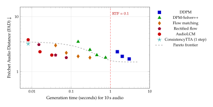
Long-Form Audio and Music Generation
The audio and music generation systems studied so far produce segments of fixed, modest duration: typically 5 to 30 seconds. This window is dictated by the model's context length (for autoregressive systems) or the latent tensor size (for diffusion and flow models), both of which are constrained by GPU memory and the quadratic cost of attention. Yet the audio that humans actually want to generate, a complete song, a podcast episode, a film soundtrack, spans minutes or hours. Bridging the gap between a model's native generation window and the durations demanded by real applications is one of the central open challenges in audio generation.
This section analyses the long-form challenge from both theoretical and practical perspectives. We begin by characterising the hierarchical structure of music and audio (The Long-Form Challenge), then examine hierarchical generation approaches (Hierarchical Approaches), autoregressive chunking with overlap (Autoregressive Chunking with Overlap), and song-level structure modelling (Song-Level Structure Modelling). The reader may find it helpful to compare these approaches with the analogous strategies for long video generation discussed in Long Video Generation.
The Long-Form Challenge
Music possesses a natural hierarchical structure spanning multiple timescales. Understanding these timescales is essential for designing systems that can generate coherent long-form content.
Definition 50 (Musical Timescale Hierarchy).
We identify five principal timescales in Western music. Five levels are separated by four gaps, each of roughly an order of magnitude, so the hierarchy spans about four decades in total, not five: from ,ms to ,min is a factor of , or decades. The band boundaries below are conventions rather than measurements, and other authors draw them somewhat differently.
Note level (50–500,ms): Individual note onsets, attacks, and decays. The pitch, duration, and dynamics of a single note.
Beat/bar level (0.5–4,s): Rhythmic patterns, chord changes, and local harmonic progressions within a measure.
Phrase level (4–16,s): Melodic phrases, harmonic cadences, and call-and-response patterns spanning several bars.
Section level (16–60,s): Verse, chorus, bridge, solo, and other structural sections of a song. Each section has a distinct harmonic, rhythmic, and textural character.
Song level (2–10,min): The overall form of a piece: the sequence of sections, the arc of tension and release, the introduction and coda.
Current generation models with a 10-second window operate comfortably at the phrase level but struggle at the section level and fail entirely at the song level. The fundamental difficulty is that coherence at higher levels requires information about events that occurred many seconds or minutes in the past.
Insight.
The information bottleneck at chunk boundaries. When generating long audio by concatenating chunks, the model must encode all relevant information about the past into a finite-dimensional conditioning signal (e.g., the last few seconds of the previous chunk, or a summary embedding). This creates an information bottleneck: details about musical form, key modulations, and thematic development are lost when they cannot be represented in the conditioning signal. The result is music that sounds locally coherent but globally aimless, lacking the large-scale structure that distinguishes a composed piece from an improvisation.
Example 25 (Timescale vs. model context).
Consider a transformer-based music generation model operating on latent tokens with a temporal compression factor of 320. At 24,kHz this is a token rate of tokens per second, so each token represents exactly ,ms of audio. With a context length of 2048 tokens, the model's receptive field spans . This is sufficient for phrase-level coherence but inadequate for maintaining section-level structure in a 4-minute song, which at 75 tokens per second is tokens. Even with an 8192-token context (a significant memory investment), the model sees , or of the song - just under half.
Round the token duration to ,ms and these figures drift: the same tokens then appear to be ,s, and four minutes appears to need tokens. Carry the exact rate of tokens per second instead; the error compounds in the attention estimate below.
Memory and compute scaling.
The computational cost of extending the generation window depends on the model architecture. For a transformer with full self-attention over tokens, the memory scales as and the compute per step as , where is the model dimension. Generating a 4-minute song at 24,kHz with compression factor 320 requires tokens. Compared to a 10-second window (), the sequence is exactly times longer, so this represents a increase in attention memory and compute. Even with linear-attention variants or sparse attention patterns, the scaling remains at least , making brute-force extension of the generation window impractical for song-length audio.
Hierarchical Approaches
One strategy for overcoming the context-length bottleneck is to generate music at multiple levels of the timescale hierarchy, using the output of coarser levels to condition finer levels. This mirrors the hierarchical approach used in long video generation (see Long Video Generation) and in cascade-based image generation.
Definition 51 (Hierarchical Music Generation).
A two-level hierarchical music generation system consists of:
A structure model that generates a compact structural representation , where is the number of structural tokens and is the token dimension. The structural representation encodes high-level attributes: section boundaries, key centers, tempo changes, and instrumentation transitions.
An audio model that generates the full audio latent conditioned on the structural plan and (optionally) the text prompt. The audio model operates at a finer temporal resolution () and is responsible for local details: note-level timing, timbre, dynamics, and mixing.
The full generation process is: (Hierarchical GEN) where is the audio codec decoder (e.g., EnCodec, DAC).
A reference design.
The following is a composite of how hierarchical systems are typically built, not a description of any one published system. The structure model is a small transformer that generates a sequence of “structure tokens” at a rate of approximately one token per bar (roughly 2 seconds of music). Each structure token encodes a low-dimensional embedding of the harmonic, rhythmic, and timbral characteristics of the corresponding bar. The structure tokens are obtained during training by applying a learned quantiser to bar-level summaries extracted from the training data.
The audio model is a larger diffusion transformer that generates the full-resolution audio latent conditioned on the structure tokens via cross-attention. Because the structure tokens span the entire song, the audio model has access to global structural information even when it generates individual chunks.
Remark 45.
Training hierarchical systems requires aligned data at both levels. The structure model needs annotations (or automatically extracted features) indicating section boundaries, chord progressions, and instrumentation changes. Obtaining such annotations at scale is challenging; current systems rely on a combination of music information retrieval (MIR) tools and self-supervised feature extraction. The quality of the structural annotations directly limits the quality of the hierarchical generation.
Proposition 35 (Hierarchical compression advantage).
Let denote the length of the audio latent sequence and the length of the structural sequence, with compression ratio . In a hierarchical system where the structure model uses full self-attention over tokens and the audio model uses full self-attention over chunks of tokens (with ), the total attention cost for generating a piece of length is (Hierarchical COST) where is the overlap between adjacent chunks. Compared to the monolithic cost , the hierarchical cost satisfies for . With one structure token per bar at 2,s the structure rate is tokens per second, against audio tokens per second, so Taking (four minutes), and , the two terms are summing to , a reduction.
Proof.
The structure model attends over tokens with full self-attention, giving cost . The audio model generates chunks, each with attention cost . Summing gives (Hierarchical COST). The ratio to follows by algebraic simplification.
Caution.
The saving does not come from the hierarchy. The two terms in the ratio differ by three orders of magnitude: against . The chunking term dominates so completely that is essentially irrelevant - halving it to moves the total from to , a change of one part in a thousand, and the reduction factor from to . Every bit of the saving is bought by refusing to attend across the whole song, which Autoregressive Chunking with Overlap obtains without any hierarchy at all.
What the structure model buys is therefore not compute but coherence: a cheap global channel through which chunk learns what chunk did. It is worth having for that reason, and this proposition should not be cited as its cost justification.
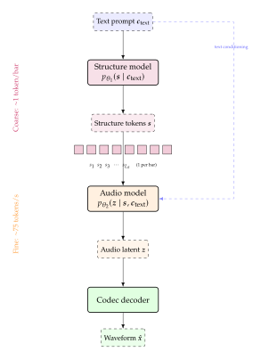
Autoregressive Chunking with Overlap
The most widely used approach to long-form audio generation is conceptually simple: generate the audio one chunk at a time, conditioning each new chunk on the tail of the previous chunk to ensure continuity at the boundary. This mirrors the autoregressive chunk generation strategy for long video (see Long Video Generation), adapted to the particular demands of audio coherence.
Let denote the -th chunk of audio (in the latent space, with tokens per chunk), and let be the overlap parameter. The generation factorises as (AR Chunk) where denotes the last tokens of chunk , and is the total number of chunks for an -token output.
Cross-fading.
The overlap region between consecutive chunks is generated twice: once as the tail of chunk and once as the head of chunk . To avoid discontinuities, the two versions are blended using a cross-fade: (Crossfade) where indexes the output stream aligned to chunk and is a linear blend weight. Note the index shift: the overlap region occupies positions of chunk but positions of chunk , since each chunk is generated in its own local coordinates. Writing in the blend would compare the tail of one chunk against the tail of the next. More sophisticated cross-fade functions (e.g., raised cosine, equal power) change the trade-off at the seam; see Exercise 17.
Proposition 36 (Overlap-add coherence).
Let and be audio chunks generated by a model with conditional distribution , and let be the cross-faded output as in (Crossfade). Define the boundary discontinuity as the mean squared disagreement per overlapped token, (Boundary DISC) and let be the “ground truth” (the audio a model with infinite context would produce). Assume the two chunks deviate from by equal amounts on average, at corresponding positions. Write for the mean squared residual per token in the overlap region after cross-fading. Then:
Unconditional bound. For any blend profile with , and with no assumption whatever about the correlation between the two chunks' errors, (Crossfade Error)
Exact value for uncorrelated errors. If in addition the two deviations are uncorrelated, then for a fade profile , (Crossfade Exact) For the linear ramp of (Crossfade), and hence .
Decay in the overlap length. For a model with stationary conditional statistics and temporal autocorrelation decaying exponentially, for constants .
Proof.
Write and for the two deviations at output position , so that and, by hypothesis, . Consistently, when the two are uncorrelated, which is the definition of .
Part (i). The map is convex and , so . Taking expectations gives at every position, hence also on average over the overlap. No independence was used.
Part (ii). Expanding, The cross term vanishes by the uncorrelatedness assumption, so what is left is the factor times . Averaging over the overlap region, in which sweeps the profile , gives (Crossfade Exact). For the linear ramp, each half contributing , so .
Part (iii). For a stationary model, the conditional variance of given the conditioning window inherits the exponential decay of the autocorrelation with distance from the conditioning boundary, and is bounded by that variance.
Caution.
is not an upper bound, in any reading. The linear cross-fade gives exactly under the independence assumption, and . Dropping the assumption only makes things worse: the assumption-free bound is , attained pointwise at the two ends of the fade, where and one chunk carries the full error alone. The value would require , which is the infimum of over all profiles, attained only by - a constant blend, which is not a cross-fade at all since it never reaches either chunk. No fade satisfying and can do better than among monotone profiles of practical interest.
Note also that must be defined per token, as in (Boundary DISC). An unnormalised squared norm over a window of tokens gains a summand for every extra token of overlap, so it would grow with for trivial reasons, and no claim of monotone decrease could survive. Even per token, monotonicity in is a modelling assumption rather than a theorem: lengthening the overlap lengthens the conditioning window, which helps, but it also extends the comparison further from the conditioning boundary, where agreement is weaker.
Example 26 (Practical chunking parameters).
Consider a latent diffusion model generating audio at 24,kHz with compression factor 320. Each chunk contains latent tokens (10,s of audio). With overlap tokens (1,s), generating a 3-minute song requires At 10 ODE steps per chunk with 15,ms per step, the total generation time is ,s, yielding RTF . The overhead from overlap is modest: of tokens are re-generated for cross-fading.
Temporal inpainting for chunk boundaries.
An alternative to cross-fading is temporal inpainting: the model generates the overlap region conditioned on both the tail of the previous chunk and the head of the next chunk (or a preliminary version of it). This produces a smoother transition because the model can “see” both sides of the boundary. The inpainting formulation treats the non-overlap regions as observed and the overlap region as latent: (Inpainting) where and are the observed segments. In practice, this posterior is approximated using the Replace-then-Denoise strategy: at each denoising step, the known regions are replaced with their noised versions, and only the overlap region is updated by the model.
Song-Level Structure Modelling
Neither hierarchical generation nor autoregressive chunking directly models the large-scale form of a song. Musical form, the arrangement of sections into a coherent whole, is a defining feature of composed music, distinguishing it from aimless improvisation. Common forms include:
AABA form: Two statements of a theme (A), a contrasting bridge (B), and a return to the theme (A). Common in jazz standards and Tin Pan Alley songs.
Verse–chorus form: Alternating verses (new lyrics over similar music) and a recurring chorus (fixed lyrics and melody). Dominant in pop and rock music.
Rondo form: A principal theme alternates with contrasting episodes: ABACADA. Common in classical music.
Through-composed: No repeated sections; the music evolves continuously. Common in art songs and some film scores.
Self-similarity matrices.
A powerful tool for analysing and imposing musical form is the self-similarity matrix (SSM). Given a sequence of feature vectors extracted from an audio recording (or generated audio), the SSM is the matrix with entries (SSM) where is a similarity kernel (e.g., cosine similarity, RBF kernel). For music with clear sectional structure, the SSM exhibits a block-diagonal pattern: elements within the same section have high similarity, and repeated sections (e.g., two occurrences of the chorus) produce off-diagonal blocks of high similarity.
Definition 52 (Structure-Conditioned Generation).
A structure-conditioned generation model takes as input a target self-similarity matrix (or an equivalent structural specification, such as a list of section labels and boundaries) and generates audio whose SSM approximates : (Structure COND GEN) where is the SSM computed from the generated audio and is a tolerance.
Remark 46.
The SSM constraint in (Structure COND GEN) can be enforced during sampling via classifier guidance. At each denoising step, the predicted clean audio is used to compute an approximate SSM , and the gradient of the Frobenius-norm discrepancy is added to the score function. This “SSM guidance” nudges the generation toward producing the desired sectional structure without retraining the model. The approach is analogous to image generation with classifier guidance, but the guiding signal is a structural property of the output rather than a class label.
Conjecture 2 (Recurrence structure improves long-form quality).
Let be a music generation model and let denote a generated song with self-similarity matrix . Define the recurrence score as (Recurrence Score) where is the set of off-diagonal high-similarity pairs beyond a phrase-length distance. We conjecture that for human-composed music, is positively correlated with human preference scores for “musical coherence” and “song-like quality”, and that explicitly maximising during generation (via guidance or reward-weighted training) improves subjective quality ratings for long-form outputs.
Remark 47.
Current state-of-the-art systems are far from achieving reliable song-level structure modelling. The principal limitations are:
Training data scarcity. Most music datasets contain short clips (10–30,s), not full songs with structural annotations. Models trained on short clips never learn the statistical patterns of large-scale form.
Evaluation metrics. Standard audio quality metrics (FAD, KL divergence, inception score) evaluate perceptual quality at short timescales and do not capture structural coherence. No widely accepted metric measures whether generated music has coherent song-level form.
Computational cost. Full-song generation at CD quality (44.1,kHz, stereo) requires handling millions of latent tokens, straining the memory and computational budgets of current hardware.
Human preferences. Human evaluation of long-form music is expensive and subjective. Listeners' assessments of structural coherence depend heavily on musical training and genre familiarity, making it difficult to obtain reliable ground-truth judgements.
Addressing these limitations is an active area of research, and we expect significant progress in the coming years as training datasets grow and evaluation methodology matures.
Multi-Track Generation and Source Separation
Music, in its most natural form, is not a monolithic waveform but a superposition of individual stems: drums, bass, vocals, keyboards, guitars, strings, and other instruments. Professional music production treats each stem separately, adjusting its volume, panning, equalization, and effects before combining the stems into a final mix. This section studies the generative modelling of multi-track music and its dual problem, source separation, from a unified probabilistic perspective.
Multi-Track Generation
Multi-track generation aims to produce a set of coherent stems that sound musically meaningful both individually and when mixed together. The simplest approach is to model the joint distribution directly, treating the multi-track audio as a single high-dimensional object. More practical approaches decompose this joint distribution into manageable factors.
Definition 53 (Multi-Track Audio Model).
A multi-track audio model generates stems (each a -sample waveform or latent sequence) conditioned on a prompt , such that:
Each stem is a plausible audio signal for its assigned instrument or role.
The mixture is a plausible musical piece.
The stems are temporally aligned: onsets, beats, and harmonic changes are synchronised across stems.
The model can be parameterised in one of three ways:
Joint: , modelling all stems simultaneously. The latent space has dimension times that of a single-stem model.
Sequential (cascade): , generating stems one at a time, each conditioned on previously generated stems.
Independent with coupling: , where is a shared latent code that enforces coherence (e.g., a harmonic plan, a rhythmic grid, or a structural skeleton generated by a separate model).
Joint generation.
The joint approach concatenates or interleaves the stems along the channel dimension: is treated as a -channel audio signal. A diffusion or flow model then generates as if it were a single multi-channel audio. The advantage is that the model can capture arbitrary dependencies between stems (e.g., the bass following the kick drum, the vocals interacting with the harmonic progression). The disadvantage is the increased dimensionality: for stems, the latent space is 4 times larger, increasing memory and compute requirements by roughly the same factor.
Sequential generation.
The sequential approach generates stems in a fixed order (e.g., drums bass harmony vocals), conditioning each new stem on the previously generated ones. This reduces the per-step dimensionality to that of a single stem but introduces an order dependence: the first stem receives no musical context from the others, which can lead to suboptimal results if the “most important” stem (often vocals or melody) is not generated first.
Example 27 (Joint vs. sequential multi-track generation).
Consider generating a 4-stem mix (drums, bass, piano, vocals) for a 10-second clip at 24,kHz with a latent compression factor of 320.
table
Comparison of joint and sequential multi-track generation
for stems, 10 seconds at 24,kHz.
Approach Latent dim NFE Time (s) Total time (s) Joint (-channel) 20 1.2 1.2 Sequential (4 stages) 20 0.3 1.2 Indep. + coupling 20 0.3 0.3 5@l@ Parallel
generation on 4 GPUs or using batched inference.
Source Separation as Inverse Generation
Source separation, the task of extracting individual stems from a mixture , is the inverse problem dual to multi-track generation. A generative model that can produce plausible stems provides a natural prior for this inverse problem, leading to a Bayesian formulation of source separation.
Proposition 37 (Separation via posterior sampling).
Let be the prior distribution over stem , learned by a pretrained generative model. Assume the mixing model is linear and noiseless: . Then the posterior distribution of stem given the mixture is (Separation Posterior) where the likelihood is (Separation Likelihood) In the two-source case (), the likelihood simplifies to , where is the prior for the second source.
Proof.
By Bayes' theorem, . The likelihood is obtained by marginalising over all other sources: where we used the deterministic mixing model . For ,
Diffusion-based source separation.
The posterior in (Separation Posterior) is intractable in general, but it can be approximated using the machinery of diffusion models. The key idea is to run the reverse diffusion process for each source while enforcing the mixture constraint at each denoising step. Concretely, at each timestep of the reverse process:
Predict the clean estimate for each source using source-specific diffusion models (or a shared model with source-class conditioning).
Project the estimates onto the mixture constraint: replace with the nearest set of signals (in norm) that sum to : (Mixture Projection) This additive correction distributes the residual equally among all sources.
Continue the reverse diffusion from the projected estimates.
Lemma 3 (Optimality of equal redistribution).
The projection in (Mixture Projection) is the orthogonal projection of the unconstrained estimates onto the affine subspace .
Proof.
We seek minimising subject to . Introducing a Lagrange multiplier for the constraint, the KKT conditions give for each . Substituting into the constraint: , so , which yields (Mixture Projection).
Remark 48.
The use of diffusion priors for inverse problems is a general technique studied in 12 for image restoration tasks (denoising, inpainting, super-resolution). Audio source separation is an instance of the same paradigm, with the “forward model” being linear mixing rather than image degradation. The mathematical framework is identical; only the domain-specific priors differ.
Algorithm 6 (Diffusion-Based Source Separation).
Input: Mixture ; pretrained score models for each source class; noise schedule ; number of steps .
Output: Estimated sources .
- for
- Initialise from noise
- for
- for
- Predict clean source
- Mixture projection:
- for
- Noise and step:
- for
- return
Style Transfer and Timbre Control
Beyond generating audio from text, many applications require transforming existing audio: changing the instrumentation of a piano recording to an orchestral arrangement, transferring the “feel” of one drum pattern to another, or converting a speaking voice to a singing voice while preserving the linguistic content. These tasks fall under the broad umbrella of audio style transfer.
Timbre transfer.
Timbre, often described as the “colour” of a sound, is the perceptual quality that distinguishes two notes of the same pitch and loudness played by different instruments. Formally, timbre encompasses all spectral and temporal characteristics not captured by pitch, loudness, and duration. Timbre transfer aims to change the timbre of an audio signal while preserving its pitch, rhythm, and temporal structure.
In the diffusion/flow framework, timbre transfer is implemented as constrained sampling: the model generates audio that matches a target timbre distribution while remaining close to the source audio in a content-preserving feature space.
Definition 54 (Audio Style Transfer via Constrained Posterior).
Let be the source audio, the target style descriptor, and a style-conditioned generative prior. The audio style transfer posterior is (Constrained Style) where is a content-preserving distance (e.g., based on pitch contour similarity, onset timing, or learned content embeddings) and controls the strength of the content constraint.
Insight.
Constrained sampling unifies style transfer tasks. Timbre transfer, genre transfer, and other audio style transfer tasks can all be formulated via (Constrained Style) by choosing an appropriate content distance . For timbre transfer, preserves pitch, onset timing, and temporal envelope while allowing spectral shape changes. For genre transfer, preserves only coarse features (harmonic progression, melodic contour, song structure) while allowing changes to rhythm, timbre, and production style. This formulation reduces style transfer to posterior sampling under a diffusion or flow prior, using the same machinery developed for inverse problems in 12.
Example 28 (Timbre transfer via diffusion inversion).
A common approach to timbre transfer uses DDIM inversion (see 19). Given a source audio latent and a target timbre description :
Invert: Run the DDIM forward process (deterministic noising) on to obtain a noise latent at the terminal timestep.
Regenerate: Run the DDIM reverse process from using the diffusion model conditioned on instead of the original conditioning.
Blend: Optionally blend the regenerated audio with the original at a controllable ratio to preserve more of the source content.
The inversion step maps the source audio to a noise-space representation that preserves content information (temporal structure, onset patterns); the regeneration step reinterprets this representation through the lens of the target timbre. The fidelity of content preservation depends on the accuracy of the DDIM inversion, which in turn depends on the number of inversion steps (more steps yield more faithful inversion).
Proposition 38 (Content preservation under DDIM inversion).
Let denote the -step DDIM inversion of a clean audio latent , and let denote the -step DDIM reverse with conditioning . Define the content preservation error when equals the original conditioning, and suppose the velocity field is Lipschitz with constant and twice differentiable along the trajectory. Then:
as .
For finite , , where is the terminal noise level.
The round trip is therefore one order better in than a single one-way DDIM traversal, whose global error is with a constant that grows like ; it is not two orders better, and in particular does not decay like .
Proof.
DDIM inversion and DDIM reversal are first-order (Euler) discretisations of the same ODE traversed in opposite directions with the same step size . For a one-way traversal, the local truncation error is per step and Grönwall's inequality amplifies the accumulated error by , giving a global error .
The round trip is better because the two traversals make opposite errors at corresponding steps. Linearising the field along the trajectory, a forward step multiplies a perturbation by and the matching reverse step by , where is the Jacobian of the field; the composition is , so each forward–reverse pair contributes a relative error of order rather than . Summing the pairs, using and approximately, for variance-preserving schedules. This is claim (ii), and (i) follows. Note that the cancellation removes one power of , not two: terms of size sum to , which is first order.
Remark 49.
The decay is the optimistic case, and it assumes the conditioning is unchanged. Style transfer deliberately changes between inversion and reversal, so the two traversals no longer follow the same field and the cancellation argument above does not apply; the error then behaves like a one-way traversal, with an constant. This is why practical timbre transfer inverts only part way, to an intermediate , rather than to full noise: a shorter trajectory both shrinks and limits how far the two fields can diverge.
Genre transfer.
Genre transfer generalises timbre transfer to higher-level musical attributes: converting a jazz piano trio performance into a rock band arrangement, or transforming an electronic dance track into an acoustic folk rendition. This requires changing not only the timbres but also the rhythmic patterns, harmonic voicings, and production style. The constrained sampling framework in (Constrained Style) applies, but the content distance must preserve only the most abstract features (overall harmonic progression, melodic contour, song structure) while allowing the model freedom to modify lower-level details.
Historical Note.
From signal processing to generative separation. Source separation has a long history in signal processing, dating back to the cocktail party problem articulated by Cherry in 1953. Classical approaches, including independent component analysis (ICA), non-negative matrix factorisation (NMF), and Wiener filtering, rely on hand-crafted signal models. The deep learning era brought supervised separation networks (e.g., Wave-U-Net, Open-Unmix, Demucs), which train discriminatively on paired mixture-source data. The generative approach studied here represents a third paradigm: using pretrained generative priors for each source, with no need for paired training data. This “zero-shot” separation capability is a direct consequence of the Bayesian duality between generation and inference, and it improves automatically as the generative models improve, without retraining the separation system.
0.50.4pt
Exercise 15 (Flow matching vs. diffusion for audio).
Consider a 1D audio latent space () with data distribution and source distribution .
Compute the optimal transport map from to .
Write down the exact velocity field for the linear interpolation flow matching model with OT coupling. Verify that it is linear in for all .
Compute the probability flow ODE velocity field for a variance-preserving diffusion model with schedule , . Show that it too is affine in - because is Gaussian here, every is Gaussian, its score is affine, and so is the velocity - but that, unlike part (b), its coefficients depend on . It is this -dependence, not any nonlinearity, that forces a fine discretisation.
Numerically integrate both velocity fields using the Euler method with steps, starting from . Compare the endpoint errors and verify that the flow matching field requires fewer steps for a given accuracy.
Exercise 16 (Consistency distillation loss).
Let be a consistency function parameterised as in (Consistency Param). Write for the noise level at time , for the noise level at the boundary , and for the data scale.
A tempting choice is , . Show that it fails the boundary condition: at it gives and , so . Then verify that the Karras-style choice does satisfy and , hence for every base network . What goes wrong in the first choice is that it measures the boundary by the ratio of noise levels rather than by their difference.
Show that the consistency distillation loss (CD LOSS) with reduces to
Explain why the EMA target network () is necessary for stable training. What happens if (no EMA)?
Exercise 17 (Overlap-add analysis for long-form audio).
A music generation model produces chunks of latent tokens with an overlap of tokens. By part (iii) of Proposition 36 the per-token boundary discontinuity obeys with tokens; normalise the constant by taking , the per-token signal power, so that is a relative error.
Derive the minimum overlap for which the bound guarantees . (Answer: tokens, about ,s at 75 tokens per second.) Explain why the answer is undetermined if is left unspecified, and why normalising by the signal power is the natural choice.
Compute the number of chunks needed to generate a 3-minute song at 24,kHz with compression factor 320, using overlap , and compare the regeneration overhead with the of Example 26.
Evaluate the fade cost of (Crossfade Exact) for three profiles: the linear ramp ; the raised cosine ; and the equal-power fade , for which the two weights are not and but and . Show that , and respectively, so that the residual errors are , and : on this metric the linear ramp is the best of the three and equal power the worst.
Audio practice nevertheless prefers the equal-power fade. Resolve the apparent contradiction by computing, at the midpoint , the amplitude of the blended signal in two regimes: when the two chunks are uncorrelated (powers add) and when they are identical (amplitudes add). Show that the linear ramp loses ,dB at the midpoint in the uncorrelated case and holds ,dB in the correlated case, while equal power holds ,dB uncorrelated and gains ,dB correlated. Which regime does Proposition 36 assume, and why does that make it the wrong guide for choosing a fade when consecutive chunks agree about the music?
Exercise 18 (Bayesian source separation).
Consider the two-source separation problem with mixture , where and are independent Gaussian sources in .
Derive the exact posterior and show that it is Gaussian. Compute its mean and covariance.
The posterior mean is the Wiener filter estimate. Express it in terms of , , , , and .
Now suppose has a non-Gaussian prior (e.g., a mixture of Gaussians representing different instrument timbres). Explain how the diffusion-based separation procedure (project-and-denoise) of Source Separation as Inverse Generation approximates the true posterior, and discuss when it might fail.
Derive the equal-redistribution projection (Mixture Projection) for the -source case as the orthogonal projection onto the affine subspace . Verify that the residual exactly.
Cross-Modal Generation
The previous sections addressed audio and music generation conditioned on text prompts, tags, or melodic hints. In many practical applications, however, the conditioning signal originates from an entirely different modality: a video stream that requires a matching soundtrack, a set of lyrics that must be sung with correct timing, or an existing audio clip that must be extended, inpainted, or super-resolved. Each of these scenarios demands architectures that bridge representational gaps between modalities while preserving the fine-grained temporal structure that characterises audio.
This section formalises three families of cross-modal audio generation: video-to-music (Video-to-Music Generation), lyrics-conditioned singing synthesis (Lyrics-Conditioned Generation), and audio-to-audio tasks such as inpainting and editing (Audio-to-Audio: Inpainting and Editing).
Video-to-Music Generation
A background music track must reflect the visual content, the emotional tone, and the temporal dynamics of its accompanying video. We begin with a precise problem statement.
Definition 55 (Video-Conditioned Music Generation).
Let be a sequence of visual feature vectors extracted from a video at frame rate , and let denote a waveform of duration seconds at sample rate . The video-conditioned music generation problem is to learn a conditional distribution (V2M Marginal) where denotes a latent representation (e.g., discrete audio tokens or a continuous latent spectrogram) and collects all learnable parameters. The model must satisfy the temporal alignment constraint: musically salient events (beat onsets, harmonic changes, dynamic swells) should correlate with visually salient events (scene cuts, motion peaks, lighting changes).
Visual feature extraction.
The visual encoder is typically a pretrained vision transformer (e.g., CLIP ViT-L/14 or DINOv2). For a video of frames, we obtain . Two strategies dominate the literature:
Frame-level features. Each frame is encoded independently, yielding . This preserves fine-grained temporal information but ignores inter-frame motion.
Clip-level features. A video encoder such as VideoMAE or TimeSformer processes short clips (e.g., 16 frames) and produces a single vector per clip. This captures motion but reduces temporal resolution.
In practice, Diff-BGM [26] and VidMuse [27] combine both: frame-level features provide a dense temporal signal, while a clip-level summary vector captures global scene semantics.
Temporal alignment mechanisms.
The mismatch between video frame rate (, typically 24 fps) and audio token rate (, often 50 Hz for neural codec tokens) necessitates an alignment module. Let denote a soft alignment matrix, where is the number of audio tokens. The aligned visual features are (V2M Align) so that each audio token position receives a weighted combination of visual features. Diff-BGM learns via cross-attention within a latent diffusion model; VidMuse employs a dedicated temporal alignment network that predicts from rhythm and motion energy signals.
Key Idea.
Rhythm-aware alignment. Music is organised around a beat grid, while video has no such intrinsic periodicity. Effective video-to-music systems first estimate the target tempo (beats per minute) from the visual motion energy, then construct so that beat positions in the audio coincide with high-motion frames in the video. This produces soundtracks that “breathe” with the visual dynamics.
Diff-BGM.
Diff-BGM [26] uses a two-stage approach:
Video analysis. A pretrained scene classifier and motion energy estimator produce a scene label sequence and a continuous arousal curve .
Conditional latent diffusion. A U-Net denoiser operates on mel-spectrogram latents (where is the compressed time dimension), conditioned on both the scene label embedding and the arousal curve via cross-attention and FiLM layers.
The training objective follows the standard latent diffusion loss: (Diffbgm LOSS) where is the noised latent and summarises the visual conditioning.
VidMuse.
VidMuse [27] extends the framework to long-form video by introducing a hierarchical conditioning scheme. A global video embedding captures scene-level semantics (genre, mood), while local frame-level embeddings guide temporal details. The generation model is a transformer-based language model over EnCodec tokens, with the visual features injected via cross-attention at every layer: (Vidmuse AR) where denotes the -th audio token and is the temporally aligned visual feature sequence from (V2M Align).
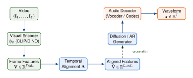
Remark 50 (Connection to audio-visual generation).
Video-to-music generation is one direction of the broader audio-visual generation problem. The reverse direction (music-to-video or audio-driven video synthesis) is treated in Audio-Visual Generation. The two directions share the temporal alignment challenge but differ in their output modalities and perceptual evaluation criteria.
Proposition 39 (Alignment optimality: the softmax is the entropy-regularised maximiser).
Let and denote the visual feature matrix and the audio hidden state matrix, respectively, and let and be the query and key projection matrices. Write for the score vector of audio position . Then:
The unregularised cross-modal attention energy is linear on the simplex , so its maximum is attained at a vertex: the energy-maximising alignment is hard attention, the one-hot vector on .
Adding a Shannon-entropy regulariser with weight makes the objective strictly concave, and its unique maximiser is the row-wise softmax: so that, stacking rows, (Align OPT)
Each row of is a probability distribution over video frames, giving a probabilistic correspondence between each audio token and the visual context. The scaling is therefore not a free normalisation constant but the weight of the entropy term: as the softmax collapses onto the hard alignment of part (i).
Proof.
(i) The cross-modal attention energy for audio position is with the -th row of . This is a linear function on a compact convex polytope, so its maximum is attained at an extreme point, and the extreme points of the probability simplex are the standard basis vectors.
(ii) Let and consider on . The entropy is strictly concave on the simplex, so is strictly concave and has a unique maximiser, which lies in the relative interior (the gradient of blows up at the boundary). Introducing a multiplier for the constraint and setting gives ; normalising yields .
Remark 51 (Why the statement needs the regulariser).
It is tempting to say that the softmax alignment maximises the attention energy. It does not: by part (i) that maximum is attained by hard attention, and the softmax is strictly suboptimal for the unregularised objective. What the softmax optimises is the energy plus an entropy bonus, which is precisely why it is the right object here: hard alignment is non-differentiable and commits irrevocably to one video frame per audio token, whereas the entropy term buys differentiability and hedging at a controlled cost in energy.
Lyrics-Conditioned Generation
Generating singing voice that matches given lyrics requires solving two intertwined problems: synthesising intelligible vocal content and producing musically coherent melodic and rhythmic patterns. This subsection analyses the conditioning mechanisms, alignment strategies, and the interplay with large-scale music models such as Jukebox (Case Study: Jukebox and Music Generation).
Character-level vs. word-level conditioning.
The choice of text granularity has significant architectural implications:
Character-level conditioning. Each character (or phoneme) is treated as a separate token, enabling fine-grained control over pronunciation and duration. The conditioning sequence is long, which increases the computational cost of cross-attention but allows the model to learn sub-word timing patterns (e.g., melisma, where a single syllable spans multiple notes).
Word-level conditioning. Each word is mapped to a single embedding vector, reducing the conditioning sequence length. This simplifies the alignment problem but sacrifices control over intra-word timing. Word-level models typically require a separate duration model to predict how many audio frames correspond to each word.
Definition 56 (Lyrics-to-Singing Alignment).
Let be a sequence of linguistic units (characters or phonemes) and be a sequence of audio frames. A lyrics-to-singing alignment is a monotone non-decreasing function such that gives the linguistic unit active at audio frame . Equivalently, defines a partition of into contiguous segments, where segment has duration .
The monotonicity constraint reflects the fact that, in normal singing, lyrics are produced in order. The duration vector with is the natural parameterisation of the alignment.
Duration modelling.
Given lyrics and a target melody contour (fundamental frequency), a duration model predicts the duration of each phoneme: (Duration Model) where is typically a small transformer or convolutional network. The predicted durations are rounded and used to expand the phoneme embeddings to the audio frame rate via repetition: (Expand)
Jukebox and VQ-VAE approaches.
Jukebox [28] demonstrated that lyrics can be incorporated as conditioning for a hierarchical VQ-VAE music model. The lyrics are encoded by a small transformer and injected via addition to the audio token embeddings at each level of the hierarchy. While Jukebox produces impressive results, the alignment between lyrics and audio is largely learned implicitly, without an explicit duration model. This leads to occasional misalignment artefacts (skipped words, repeated phrases) that more structured approaches avoid.
Example 29 (Lyrics conditioning in Jukebox).
In Jukebox, the lyrics encoder produces a sequence of embeddings . These are aligned to the audio token sequence via a learned attention mechanism at each level of the VQ-VAE hierarchy. Jukebox operates at Hz with encoder hop sizes of , and samples, so the three levels carry tokens at At the top level (lowest resolution, 344 Hz) the attention is coarse and captures phrase-level alignment; at the bottom level (highest resolution, 5.5 kHz) it refines to phoneme-level alignment. Note that no level runs at the audio sample rate: even the finest codebook is a downsampled token stream, not a waveform. The hierarchical structure allows the model to capture both global lyrical structure and local pronunciation details.
Insight.
Monotonic attention for lyrics alignment. Standard soft attention allows the model to attend to any position in the lyrics at any point in time, which can produce non-monotonic alignments (e.g., singing words out of order). Enforcing monotonicity through mechanisms such as monotonic attention [3] or the Connectionist Temporal Classification (CTC) loss significantly improves alignment quality. The trade-off is reduced flexibility: monotonic attention cannot handle musical structures where lyrics are intentionally repeated or reordered (as in some choral works).
Audio-to-Audio: Inpainting and Editing
Audio-to-audio generation encompasses tasks where both the input and output are audio signals: inpainting missing regions, extending existing clips, performing super-resolution, and making localised edits. These tasks are unified by conditioning the generation on a partially observed audio signal.
Definition 57 (Audio Inpainting).
Let be a complete audio signal and let denote the set of observed sample indices, with the missing indices. The audio inpainting problem is to sample from the conditional distribution (Inpainting EDIT) where is an optional auxiliary conditioning signal (text description, surrounding context features). The inpainted signal must be (i) perceptually natural, (ii) temporally consistent with the observed regions at the boundaries, and (iii) semantically consistent with the conditioning .
Diffusion-based inpainting.
In the diffusion framework, inpainting is implemented by constraining the observed region at each denoising step. Let be the forward diffusion at time . At each reverse step, after computing the denoised estimate from the network prediction, we replace the observed region with the corresponding noised observation: (Inpaint Replace) where is the standard reverse-step output and is fresh noise. This repaint strategy [4] ensures the observed region remains faithful to the input throughout the denoising process.
Remark 52 (Boundary artefacts in naive inpainting).
The replacement strategy in (Inpaint Replace) can create discontinuities at the boundary between and , because the generated region and the observed region evolve under different noise schedules during the reverse process. Several remedies exist: (i) applying a smooth transition mask at the boundary, (ii) resampling several denoising steps (the “repaint” jumps of [4]), or (iii) using a harmonisation network that post-processes the boundary.
Audio super-resolution.
Super-resolution is a special case of audio-to-audio generation where corresponds to the low-frequency content. Given a band-limited signal with bandwidth , the goal is to synthesise the high-frequency band conditioned on . In the frequency domain, this can be formulated as (Superres) where is a generative model for the missing bandwidth.
Audio extension (outpainting).
Audio extension (also called outpainting or continuation) generates new audio that seamlessly continues an existing clip. Formally, given , we wish to sample . Autoregressive models handle this naturally by simply continuing the token generation. For diffusion models, the continuation is treated as a right-boundary inpainting problem: the observed region is and the missing region is .
Example 30 (Instruction-based audio editing).
Instruction-based audio editing systems (e.g., InstructME, AUDIT) accept a source audio clip and a natural language instruction such as “remove the drums” or “add reverb to the vocals.” The system must identify the relevant audio region, apply the requested modification, and leave the remaining content unchanged. This requires a joint understanding of audio semantics and natural language, typically achieved by conditioning a diffusion model on both the source audio and a text embedding of the instruction: (Instruct EDIT) The conditioning on is implemented via concatenation in the input channels of the U-Net denoiser, while is injected through cross-attention.
Proposition 40 (Inpainting as constrained posterior sampling).
Let be the prior distribution of complete audio signals. The audio inpainting posterior decomposes as (Inpaint Bayes) When the prior is modelled by a diffusion model, sampling from this posterior requires running the reverse process while constraining the observed indices. The replacement strategy in (Inpaint Replace) approximates this posterior sampling by enforcing the observation constraint at each step.
Proof.
The decomposition in (Inpaint Bayes) follows directly from the definition of conditional probability, and is exact. The diffusion realisation is not. What the replacement step samples at reverse step is (Inpaint Factor) where is the forward-process marginal, which is Gaussian and can be sampled exactly. This is an approximation of , not an identity: the observed block is resampled from the unconditional forward marginal, which ignores entirely, while the missing block is denoised from a whose observed half was pasted in at the previous step and therefore carries no information about what the model just generated. The two halves are consequently harmonised only through subsequent steps. This is exactly the mismatch identified in Remark 52, and it is why RePaint-style samplers add resampling jumps - repeatedly renoising back to and denoising again - to let the missing region absorb the boundary condition before the noise level drops.
Symbolic Music Generation
All generation methods discussed so far operate on audio waveforms or their spectral representations. An older but complementary tradition represents music symbolically, as sequences of discrete note events. Symbolic representations capture pitch, timing, duration, and velocity with exact precision, at the cost of discarding timbre, room acoustics, and performance nuances. This section covers the dominant symbolic representation (MIDI), transformer-based generation models, and recent diffusion approaches that operate directly on piano-roll matrices.
MIDI and Symbolic Representations
The Musical Instrument Digital Interface (MIDI) standard, introduced in 1983, remains the most widely used symbolic music representation. A MIDI file encodes a piece of music as a sequence of timestamped events.
Definition 58 (MIDI Event Sequence).
A MIDI event sequence is an ordered list of events , where each event is a tuple (MIDI Event) with:
: the timestamp (in ticks or seconds),
: the event type,
: the MIDI pitch number (where 60 = middle C, 69 = A4 = 440,Hz),
: the velocity (loudness), and
: the MIDI channel (instrument track).
Events are ordered by timestamp: .
Piano roll representation.
For computational purposes, it is often convenient to convert a MIDI event sequence into a piano roll: a binary matrix that indicates which pitches are active at each time step.
Definition 59 (Piano Roll).
Given a MIDI event sequence with a fixed time quantisation of (e.g., a sixteenth note), the piano roll is a binary matrix (Pianoroll) where is the number of time steps and if and only if pitch is sounding at time step . The piano roll can be augmented with velocity information by replacing binary values with , yielding a continuous-valued piano roll.
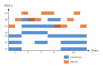
Alternative symbolic encodings.
Several alternatives to the raw MIDI event sequence have been proposed to improve the efficiency and learnability of symbolic music models:
REMI (REvamped MIDI-derived) [5]: Introduces explicit bar and position tokens, encoding each note as a sequence of sub-tokens:
[Bar],[Position],[Pitch],[Duration],[Velocity]. This makes the bar structure explicit and improves long-range coherence.Compound Word (CP) [6]: Groups the sub-tokens of REMI into a single compound token, where each compound token is a concatenation of embeddings for position, pitch, duration, and velocity. This reduces the sequence length by a factor of 4–5 compared to REMI.
Octuple [7]: Extends the compound word idea to eight attributes (time, bar, position, instrument, pitch, duration, velocity, tempo), enabling multi-track representation in a single token per note.
Remark 53 (Sequence length trade-offs).
A 4-minute piano piece at sixteenth-note resolution contains roughly
time steps. In the raw MIDI event representation, each
note requires at least two events (note_on and
note_off), and a typical piece has 1000–3000 notes,
yielding sequences of 2000–6000 tokens. The REMI encoding expands
this further (5 sub-tokens per note), while the Compound Word encoding
compresses it back to one compound token per note. These sequence
lengths are well within the capacity of modern transformers with
relative or rotary positional encodings, but they highlight the
importance of efficient tokenisation for symbolic music.
Transformer Models for Symbolic Music
The application of transformer architectures to symbolic music generation has been remarkably successful. The key insight is that a MIDI token sequence, after appropriate encoding, is structurally similar to a natural language sentence: it is a sequence of discrete tokens with both local dependencies (notes within a chord) and long-range dependencies (harmonic progressions, melodic repetitions, verse-chorus structures). We refer the reader to 17 for the general treatment of autoregressive models.
Music Transformer.
The Music Transformer [29] adapts the transformer decoder architecture for symbolic music generation, with one crucial modification: relative attention.
Standard absolute positional encodings (sinusoidal or learned) add a fixed position-dependent bias to each token. In music, however, the important relationships are often relative: a perfect fifth interval (7 semitones) has the same harmonic character regardless of its absolute pitch, and a rhythmic pattern at the beginning of a phrase has the same metrical function when it recurs four bars later.
Definition 60 (Relative Attention for Music).
Let be the query, key, and value matrices for a sequence of length . The relative attention mechanism computes (Relattn) where is the relative position bias matrix with entries (Relattn Entry) and is a learned embedding for relative position offset . To keep the number of parameters finite, offsets are clipped to .
Proposition 41 (Relative attention captures periodic structure).
Let for all (a constant query, representing a repeated motif) and suppose the relative embeddings are periodic: for some period and all . Then the relative attention scores satisfy (Periodic Score) i.e., the attention pattern is periodic with the same period . In particular, if corresponds to one bar of music, the model naturally attends to the same metrical position in all bars.
Proof.
By definition, and , where the last equality uses the periodicity of .
Compound word tokenisation.
As noted in the previous subsection, the Compound Word (CP) encoding [6] represents each musical note as a single compound token, where each compound token consists of multiple attribute embeddings that are summed or concatenated: (Compound) where each is a learned embedding for the corresponding attribute. The transformer then operates on the compound sequence , with separate prediction heads for each attribute at the output.
Example 31 (Pop music generation with compound words).
The Compound Word Transformer [6] trains a 12-layer transformer on the AILabs.tw Pop1K7 dataset (roughly 1,700 transcribed pop-piano performances, about 108 hours) using CP encoding. (Pop1K7 should not be confused with POP909, a separate 909-song piano-arrangement dataset, nor the CP paper with the earlier Pop Music Transformer, which uses the REMI encoding [5].) At generation time, the model produces a sequence of compound tokens autoregressively, predicting all attributes of each note in parallel at each step. The generated pieces exhibit clear verse-chorus structure, appropriate chord progressions, and rhythmic consistency over spans of 30–60 seconds. Beyond this duration, the model tends to drift harmonically, a limitation shared by most fixed-context-window autoregressive approaches.
Longer context and hierarchical generation.
Standard transformer architectures with context window can capture dependencies spanning at most tokens. For a CP-encoded piece, covers approximately 2 minutes of music. To generate longer pieces, several strategies have been explored:
Sliding window with memory. The model generates in overlapping windows, carrying forward a compressed memory (e.g., the hidden states of the last tokens).
Hierarchical generation. A high-level model generates a structural plan (e.g., chord progression, section labels), and a low-level model fills in the notes conditioned on this plan. This decomposes long-range structure from local note-level detail.
Sparse attention. Attention patterns such as Longformer or BigBird allow the model to attend to distant tokens at reduced computational cost, extending the effective context to tens of thousands of tokens.
Diffusion for Symbolic Music
While autoregressive transformers have been the dominant paradigm for symbolic music, diffusion models offer an attractive alternative: they can generate all time steps in parallel and naturally handle tasks like inpainting and arrangement. The challenge is that the piano roll is a discrete object, whereas standard diffusion operates on continuous spaces.
Definition 61 (Symbolic Music Diffusion).
Let be a relaxed (continuous) piano roll, obtained by treating each entry as the probability that pitch is active at time . The symbolic music diffusion model defines a forward process (SYM Forward) and a learned reverse process (SYM Reverse) where is parameterised by a neural network (typically a U-Net operating on the “image”). At generation time, the continuous output is binarised by thresholding at 0.5 to recover a valid piano roll.
Challenges of the discrete nature.
The relaxation from to introduces a mismatch between the training data (binary piano rolls) and the diffusion process (continuous). Several issues arise:
Boundary effects. The Gaussian noise process can push values outside , requiring clipping or a sigmoid transformation.
Thresholding artefacts. The binarisation step at generation time is non-differentiable and can produce noisy results near the 0.5 threshold.
Sparse activations. A typical piano roll is very sparse: at any given time step, at most 10–15 of the 128 pitches are active (and usually fewer than 6). The diffusion model must learn to produce sharp, sparse outputs from a dense Gaussian process.
Remark 54 (Discrete diffusion alternatives).
An alternative to the continuous relaxation is to use discrete diffusion models that operate directly on binary or categorical data; see sec:diffusion_language for a general treatment. D3PM [8] and related methods define forward processes that corrupt discrete tokens via transition matrices rather than Gaussian noise. For piano rolls, the absorbing-state variant is natural: each pitch independently transitions to an “unknown” state with probability that increases over the forward process, and the reverse process learns to reconstruct the original binary values.
Architecture considerations.
The piano roll is a two-dimensional structure that can be treated as a single-channel image. This observation motivates the use of 2D U-Net architectures, where the “height” dimension is pitch and the “width” dimension is time. However, the two axes have very different semantics:
The pitch axis has harmonic structure: notes separated by octaves (12 semitones) have similar function, and common intervals (thirds, fifths, octaves) have characteristic sizes.
The time axis has rhythmic structure: events are organised around a metrical grid (bars, beats, subdivisions).
Effective architectures exploit these distinct structures through asymmetric kernel sizes, separate pitch and time attention layers, or hybrid convolutional-attention designs.
Proposition 42 (Sparsity-aware loss for piano roll diffusion).
Let denote the average activation rate of the piano roll, with in practice ( for typical piano music). The standard MSE diffusion loss treats active and inactive entries equally. A reweighted loss that upweights active entries by improves reconstruction of the sparse active notes: (Sparse LOSS) where and . This is equivalent to optimising a weighted Gaussian log-likelihood where the variance is scaled inversely with class frequency.
Proof.
The standard MSE loss assigns equal weight to all entries. Since a fraction of entries are active and are inactive, the gradient contribution from active entries is proportional to , which is small. Setting ensures that the total weight on active entries equals the total weight on inactive entries: . This balances the gradient contributions and prevents the model from learning a trivial all-zeros prediction.
Example 32 (Piano roll diffusion for accompaniment generation).
Consider generating an accompaniment piano roll conditioned on a given melody piano roll . This is a conditional generation task where the conditioning signal has the same dimensionality as the output. The conditioning is implemented by concatenating as an additional input channel to the U-Net: (Accomp COND) where denotes channel-wise concatenation. The generated accompaniment respects the harmonic context of the melody, producing chords and bass lines that are harmonically consistent.
Commercial and Industrial Systems
The research advances described in previous sections have been translated into commercial products that can generate full-length songs, complete with vocals, lyrics, instrumentation, and mixing. This section surveys the major commercial and industrial systems as of 2024–2025, analyses their known (or inferred) architectures, and provides a comparative evaluation. We emphasise that many of these systems are closed-source, so the architectural details presented here are based on published papers, patent filings, blog posts, and empirical observation.
Caution.
Closed-source limitations. The commercial systems described in this section are proprietary. Architectural details are inferred from published information and may not reflect the actual implementations. Quantitative comparisons should be interpreted with caution, as the systems are continually updated and the evaluation conditions may differ. We include this section because these systems represent the state of the art in user-facing music generation and illustrate the practical engineering decisions that complement the theoretical foundations developed earlier.
Google MusicLM / MusicFX
MusicLM [30] was one of the first systems to demonstrate high-quality, long-form text-to-music generation. Its architecture exemplifies the hierarchical token generation paradigm that has become the dominant approach for audio generation at scale.
Architecture overview.
MusicLM uses a three-stage hierarchical generation process:
Semantic tokens. A first transformer maps a text description to a sequence of semantic tokens. These tokens are not MuLan outputs: they are obtained by -means quantising the intermediate representations of a self-supervised speech/audio model, w2v-BERT, at a coarse temporal resolution (25,Hz), and they capture high-level musical attributes (genre, mood, instrumentation, melodic contour). MuLan [9] plays a different role: it is a joint text-audio embedding model (analogous to CLIP for text-image), trained on 44M audio-text pairs, whose quantised embedding supplies the conditioning prefix for this stage. At training time the MuLan audio embedding of the target clip is used; at inference time the MuLan text embedding of the prompt is substituted, which is what removes the need for paired text-music training data.
Coarse acoustic tokens. A second transformer maps the semantic tokens to coarse acoustic tokens from a SoundStream [10] neural audio codec. These tokens encode the broad spectral shape and harmonic content at 50,Hz.
Fine acoustic tokens. A third transformer (or the same transformer with a different head) refines the coarse tokens by predicting the residual quantisation levels of the codec, capturing fine spectral detail and high-frequency content.
The full generation pipeline can be written as (Musiclm Hierarchy) where denotes semantic tokens, coarse acoustic tokens, fine acoustic tokens, and the output waveform.
MuLan conditioning.
The MuLan model projects both text and audio into a shared embedding space , trained with a contrastive loss: (Mulan LOSS) where and are the text and audio encoders, is the batch size, and is a temperature parameter. At generation time, the text is encoded by , and the resulting embedding conditions the semantic token generator.
MusicFX and Gemini-era updates.
Following MusicLM, Google released MusicFX as a user-facing product integrated with the Gemini family of models. Key improvements include:
Longer generation. MusicFX supports generation of up to 70 seconds (compared to MusicLM's 30 seconds), achieved through sliding-window generation with overlapping context.
Improved conditioning. The MuLan embedding is supplemented with T5 text embeddings, providing richer semantic conditioning for complex prompts.
Quality filtering. A MuLan-based quality classifier filters generated candidates, selecting the output with the highest text-audio alignment score. For a batch of candidates, the selected output is (Quality Filter)
Historical Note.
From MusicLM to MusicFX. MusicLM (January 2023) established the three-stage hierarchical paradigm and demonstrated that text-to-music generation could achieve quality comparable to real recordings for short clips. MusicFX (late 2023, updated 2024) refined this approach for production use, incorporating safety filters (to avoid generating copyrighted material or harmful content), latency optimisations (streaming the coarse-to-fine stages), and user interface features (prompt suggestions, style controls). The Gemini integration (2024–2025) further improved prompt understanding by leveraging the LLM's reasoning capabilities to expand and disambiguate user prompts before feeding them to the music generation pipeline.
Suno
Suno (versions 3 through 4) is a commercial system that generates complete songs with vocals, lyrics, and full instrumentation. It represents a significant leap in scope compared to earlier systems that focused on instrumental music or short clips.
Inferred architecture.
Based on public information and empirical analysis, Suno appears to employ a two-stage architecture:
Structure planning. Given a text prompt (or user-provided lyrics), a language model generates a structural plan that specifies: itemize
Song structure (intro, verse, chorus, bridge, outro),
Lyrical content for each section (if not user-provided),
Approximate duration and tempo,
Genre and stylistic tags. itemize This stage can be understood as sampling from a conditional distribution over structural descriptions: (SUNO Structure) where encodes the song structure and is the user's input.
Audio synthesis. A second model generates the audio waveform conditioned on the structural plan: (SUNO Synthesis) This stage likely combines a transformer-based token generator (for coarse structure) with a diffusion-based refinement stage (for high-fidelity audio). The vocal track and instrumental track may be generated jointly or in separate streams that are mixed in a final step.
Full-song generation.
A distinguishing feature of Suno is its ability to generate songs of 2–4 minutes in length with coherent large-scale structure. This requires:
Long-range coherence. The model must maintain harmonic, melodic, and rhythmic consistency across the entire song. The structure planning stage addresses this by providing a high-level blueprint.
Vocal-instrumental alignment. The generated vocals must be synchronised with the instrumental accompaniment, both in timing (lyrics align with the beat) and in pitch (vocals follow the chord progression).
Dynamic range. Real songs have dynamics (quiet verses, loud choruses). The model must vary energy, density, and spectral content across sections.
Remark 55 (Training data considerations).
The training data for Suno reportedly includes a large corpus of licensed and/or public-domain music. The scale and composition of this dataset are significant factors in the system's performance. Copyright concerns surrounding AI-generated music trained on copyrighted material remain an active legal and ethical issue that is beyond the scope of this text.
Udio
Udio, developed by former members of Google DeepMind, is a competing commercial system that also generates full songs with vocals and instrumentation.
Architecture overview.
Udio's architecture is believed to centre on a diffusion-based generation model operating in a latent space, conditioned on text embeddings from a large language model. Key design choices (inferred from public demonstrations and interviews) include:
Latent diffusion. Audio is encoded into a compressed latent space via a neural audio codec, and the diffusion process operates in this latent space (similar to the approach of AudioLDM and Stable Audio).
LLM-based text understanding. The text prompt is processed by a large language model that extracts structured attributes (genre, mood, tempo, instrumentation) before conditioning the diffusion model.
Iterative refinement. The generation may involve multiple passes: a first pass generates a draft, and subsequent passes refine specific aspects (vocal clarity, instrumental balance, dynamic range).
Comparison with Suno.
While both systems target the same use case (full-song generation from text prompts or lyrics), empirical evaluations by users and independent reviewers suggest the following qualitative differences:
Vocal quality. Suno tends to produce more natural-sounding vocals with better pronunciation, while Udio excels at certain vocal styles (e.g., operatic, choral).
Instrumental variety. Udio shows greater diversity in instrumentation and arrangement, particularly for genres outside mainstream pop.
Structural coherence. Both systems occasionally produce songs with structural anomalies (e.g., abrupt endings, missing transitions), though the rate of such anomalies has decreased with successive versions.
Comparative Analysis
We summarise the key features of the major commercial and research systems in the following table.
1.2
System Dur. Vocals Conditioning Architecture Open Year MusicLM 30,s No Text (MuLan) Hier. AR No 2023 MusicGen 30,s No Text (T5) Single AR Yes 2023 AudioLDM 2 10,s No Text (CLAP+GPT2) Latent diff. Yes 2023 Stable Audio 95,s No Text (CLAP) Latent diff. Partial 2024 Suno v3/v4 240,s Yes Text / lyrics AR + diff. No 2024 Udio 240,s Yes Text / lyrics Latent diff. No 2024 MusicFX 70,s No Text (MuLan+T5) Hier. AR No 2024
Remark 56 (Rapid evolution).
The commercial music generation landscape evolves rapidly. Between 2023 and 2025, the maximum generation duration increased from 30 seconds to over 4 minutes, vocal synthesis went from non-existent to near-human quality, and the number of controllable parameters (genre, mood, tempo, instrumentation, structure) expanded considerably. Any snapshot comparison, including the one above, is likely outdated by the time it is read. The reader is encouraged to consult online benchmarks and user evaluations for the most current comparisons.
Insight.
The two-stage pattern. A recurring architectural pattern in commercial systems is the separation of planning (generating a high-level structural description) from synthesis (generating the audio waveform conditioned on the plan). This mirrors the plan-then-execute paradigm in language model agents and reflects a fundamental principle: long-range coherence is better achieved by planning at a coarse temporal resolution than by attempting to maintain it through thousands of fine-grained autoregressive steps.
Evaluation Metrics for Audio Generation
Evaluating generated audio is challenging because perceptual quality, fidelity to a conditioning signal, and musical coherence are all multidimensional attributes that resist reduction to a single number. This section provides a rigorous treatment of the major evaluation metrics used in the audio generation literature, including their mathematical definitions, statistical properties, and practical limitations.
Fréchet Audio Distance
The Fréchet Audio Distance (FAD) is the audio analogue of the Fréchet Inception Distance (FID) used in image generation. It measures the distance between the distribution of real audio and the distribution of generated audio in a learned feature space.
Definition 62 (Fréchet Audio Distance).
Let and be sets of real and generated audio clips, respectively. Let be a feature extractor (e.g., VGGish) that maps each audio clip to a -dimensional embedding. Compute the feature statistics: (FAD Stats R) The Fréchet Audio Distance is (FAD)
The matrix square root is the unique positive semidefinite matrix satisfying . When and commute (i.e., share the same eigenvectors), this simplifies to the element-wise square root of their eigenvalue products.
Theorem 3 (FAD as between Gaussians).
The FAD is equal to the squared -Wasserstein distance between two multivariate Gaussian distributions: (FAD W2) In particular, with equality if and only if and .
Proof.
The squared -Wasserstein distance between two probability measures and on is (W2 DEF) where is the set of all couplings of and . For Gaussians and , the optimal transport map is the affine map , where . Substituting and simplifying (see 14 for the general theory of optimal transport), we obtain (W2 Gaussian) where the last equality uses the identity , which follows from the cyclic property of the trace and the fact that and have the same nonzero eigenvalues for any matrix . Setting and recovers (FAD).
Non-negativity follows from the general property . For the equality case, if and only if the two distributions are identical, which for Gaussians requires and .
Feature extractors for FAD.
The choice of feature extractor significantly affects the FAD score:
VGGish [11]: A CNN trained on AudioSet for audio event classification. This is the most common choice but may not capture music-specific features (melody, harmony, rhythm) effectively.
PANN (PANNs-CNN14): A larger CNN also trained on AudioSet, providing a richer feature space () compared to VGGish ().
CLAP embeddings: Using the audio encoder of a CLAP model as yields a FAD variant that is sensitive to semantic audio attributes. This variant is sometimes called the “CLAP-FAD.”
EnCodec features: Using intermediate representations from a neural audio codec captures perceptual quality at a fine-grained level.
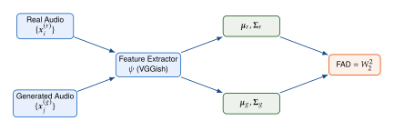
Remark 57 (Sample size effects on FAD).
The FAD estimate is biased upward: with finite samples both the means and the covariances are estimated with error, and both errors inflate the score. The mean term's bias is exactly computable. If the features are i.i.d. with covariances , then and are independent with covariances and , so (FAD BIAS) Subtracting the last two terms removes the bias of the mean term exactly. Note that this is not : the correction is proportional to the total feature variance, not to the feature dimension, and the two agree only if every feature coordinate happens to have unit variance. The covariance term's bias has no comparably simple closed form - it depends on the spectrum of - but it is also in order of magnitude, so FAD grows badly with the feature dimension at fixed . In practice the safe protocol is therefore not a correction formula at all: fix and across every system being compared, report them, and if an -independent number is wanted, evaluate FAD at several sample sizes and extrapolate the fitted line in to . For VGGish (), is a common minimum; for higher-dimensional extractors, more samples are needed.
Perceptual Quality Metrics
Unlike distributional metrics such as FAD that compare populations of audio clips, perceptual quality metrics evaluate individual audio signals against a reference or in isolation.
Definition 63 (PESQ: Perceptual Evaluation of Speech Quality).
The Perceptual Evaluation of Speech Quality (PESQ; ITU-T P.862) is a full-reference metric that compares a degraded signal against a clean reference . The PESQ algorithm operates as follows:
Level and time alignment. Both signals are level-adjusted and temporally aligned using a correlation-based delay estimator.
Perceptual modelling. Both signals are transformed to a perceptual domain using a model of the human auditory system, yielding loudness-density representations (time-frequency with Bark-scale frequency resolution).
Disturbance computation. The signed disturbance is , decomposed into positive (additive) and negative (subtractive) components.
Aggregation. The disturbances are aggregated over time and frequency using Minkowski norms to yield the PESQ score: (PESQ) where and are the symmetric and asymmetric disturbance measures, and are regression coefficients calibrated against human judgments.
The PESQ score ranges from to , with higher values indicating better quality.
Definition 64 (ViSQOL: Virtual Speech Quality Objective Listener).
ViSQOL [12] is a full-reference metric designed for a broader range of audio signals (not just speech). It operates by:
Computing gammatone spectrograms of the reference and degraded signals.
Extracting neurogram similarity index measure (NSIM) patches, which compare local spectro-temporal patterns using a structural similarity index.
Aggregating patch similarities across the signal to produce a MOS-LQO (Mean Opinion Score, Listening Quality Objective) estimate on a 1–5 scale.
Definition 65 (PEAQ: Perceptual Evaluation of Audio Quality).
PEAQ (ITU-R BS.1387) is a full-reference metric designed for general audio (music, speech, environmental sounds). It computes multiple model output variables (MOVs) including:
Bandwidth differences between reference and test signals,
Noise-to-mask ratio (NMR): the ratio of distortion energy to the masking threshold at each time-frequency point,
Harmonic structure of distortions,
Temporal envelope differences.
These MOVs are combined by a neural network trained on subjective test data to produce an Objective Difference Grade (ODG) on a scale from (very annoying) to (imperceptible difference).
Remark 58 (Applicability to generated audio).
PESQ, ViSQOL, and PEAQ are full-reference metrics: they require a clean reference signal to compare against. For audio generation tasks, a reference signal often does not exist (the generated audio is novel). These metrics are therefore most applicable to:
Codec evaluation. Comparing the output of a neural audio codec (e.g., EnCodec) against the original input.
Enhancement tasks. Evaluating denoising, super-resolution, or bandwidth extension where a clean reference is available.
Reconstruction quality. In VAE-based systems, comparing the reconstruction against the original .
For unconditional or text-conditioned generation, reference-free metrics (see below) or human evaluation are more appropriate.
CLAP Score
The CLAP (Contrastive Language-Audio Pretraining) score measures the alignment between a generated audio clip and its conditioning text prompt, analogous to the CLIP score in image generation.
Definition 66 (CLAP Score).
Let and be the text and audio encoders of a pretrained CLAP model, with the shared embedding dimension. The CLAP score for a text-audio pair is the cosine similarity of their embeddings: (CLAP Score EVAL) The average CLAP score over a test set of text-audio pairs is (CLAP AVG)
The CLAP score is related to the CLAP contrastive loss (CLAP: Contrastive Language–Audio Pretraining) used during CLAP pretraining. A higher CLAP score indicates that the generated audio is more semantically aligned with the text description.
Proposition 43 (CLAP score and generation likelihood).
Under the assumption that the CLAP model defines a Gibbs distribution over audio given text, (CLAP Gibbs) where is the temperature, the CLAP score is proportional to the log-likelihood: (CLAP Loglik) where is the partition function.
The prefactor depends on through , so the CLAP score is not in general a monotone transform of , and maximising the two is not the same problem. The two do coincide when the audio embeddings are -normalised, for all : then the prefactor is a positive constant for a fixed prompt, and (CLAP Argmax) This is the case in the CLAP implementations used for evaluation, which normalise both towers' outputs. Without that normalisation the energy , not the cosine similarity, is the quantity tied to the likelihood, and a generator can raise its cosine score while lowering its CLAP-model likelihood by shrinking .
Proof.
From (CLAP Gibbs), . Rearranging and dividing by : which is exactly (CLAP Loglik). For the equivalence of maximisers, if for every , the map is affine with positive slope for fixed , hence strictly increasing, so it preserves argmaxima; this gives (CLAP Argmax). If instead varies, take any with and sufficiently larger than : then has the higher likelihood but the lower cosine score, so no monotone relation can hold.
Mean Opinion Score
Despite the development of numerous objective metrics, subjective human evaluation remains the gold standard for assessing audio quality and musicality. The Mean Opinion Score is the most widely used protocol.
Definition 67 (Mean Opinion Score).
In a Mean Opinion Score (MOS) evaluation, human raters each assign an integer score to each of audio stimuli, where the scale is:
| Score | Quality |
| 5 | Excellent |
| 4 | Good |
| 3 | Fair |
| 2 | Poor |
| 1 | Bad |
Confidence intervals.
Under the assumption that the ratings for stimulus are i.i.d. draws from a distribution with mean and variance , the confidence interval for is (MOS CI) where is the sample standard deviation. The i.i.d. assumption is often violated in practice (raters have different internal scales and biases), which motivates more sophisticated analysis methods.
MUSHRA protocol.
The MUltiple Stimuli with Hidden Reference and Anchor (MUSHRA; ITU-R BS.1534) protocol is a variant designed for evaluating intermediate-quality audio (such as codec outputs or generated music). Key features include:
A hidden reference (the original high-quality audio) is included among the test stimuli.
A low-quality anchor (e.g., 3.5,kHz low-pass filtered version) is included to calibrate the scale.
Raters assign scores on a continuous 0–100 scale rather than a discrete 1–5 scale.
Raters can switch between stimuli in real time.
The MUSHRA score for stimulus is (Mushra)
Statistical testing.
To determine whether two systems produce significantly different quality, we use the Wilcoxon signed-rank test, which is appropriate for paired ordinal data and does not assume normality.
Definition 68 (Wilcoxon Signed-Rank Test for MOS Comparison).
Given paired MOS scores for systems and on stimuli, compute the differences , discard any , and rank the remaining values. The test statistic is (Wilcoxon) where is the rank of . Under the null hypothesis , the distribution of is known (tabulated for small , approximately normal for large with mean and variance , where is the number of non-zero differences). We reject at significance level if the -value .
Example 33 (MOS comparison of two music generation systems).
Suppose we evaluate systems and on prompts with raters each. The grand MOS scores are and (95% confidence intervals). The Wilcoxon signed-rank test on the per-stimulus MOS differences yields , . At the significance level, we reject the null hypothesis and conclude that system produces significantly higher-rated output than system . Note that statistical significance is not the same as practical significance: on a 5-point scale one quality category is , so a MOS difference of is about one fifth of a category. With prompts and raters, differences of this size are detectable but small, and they are routinely swamped by rater-pool and stimulus-selection effects between studies. Report the effect size alongside the -value.
Evaluation Summary
We summarise the major evaluation metrics and their properties in the following table.
1.2
Metric Type Reference Measures Scale Automated FAD Distributional Population Fidelity Yes CLAP Score Pairwise None Text alignment Yes PESQ Pairwise Full Speech quality Yes ViSQOL Pairwise Full Audio quality Yes PEAQ (ODG) Pairwise Full Audio quality Yes MOS Absolute None Overall quality No MUSHRA Comparative Hidden Audio quality No
Caution.
No single metric suffices. Each evaluation metric captures a different aspect of audio quality. FAD measures distributional similarity but is insensitive to per-sample quality variations. The CLAP score measures text-audio alignment but does not assess perceptual quality. PESQ and ViSQOL require a reference and focus on signal-level distortions rather than musical attributes. MOS captures overall quality but is expensive, subjective, and difficult to reproduce across studies. A thorough evaluation of an audio generation system should report multiple metrics (at minimum FAD, CLAP score, and MOS) and clearly describe the evaluation protocol, including the number of samples, the feature extractor used for FAD, the CLAP model version, and the MOS rater pool characteristics. Relying on a single metric is a common source of misleading conclusions in the literature.
Proposition 44 (Metric disagreement).
Let per-sample quality be measured by any functional of the form with maximised on the modes of the real distribution - the idealisation of what a listener panel scores. Then FAD and are not ordinally equivalent: there exist generators and with
Proof.
It suffices to exhibit one pair, and a one-dimensional feature space is enough. Take with density , and take the per-sample quality to be , so that a clip scores well exactly when it looks typical of real audio. Let system match the real distribution exactly, , and let system be mode-collapsed, with . Then, by (FAD), so wins on FAD. For the quality functional, so for all sufficiently small , and wins on per-sample quality.
The mechanism is the audio analogue of the precision–recall trade-off in image generation: FAD is a distributional metric that charges a system for missing modes, whereas a per-stimulus rating never sees the modes a system failed to produce. A mode-collapsed generator that always emits one impeccable piano loop can therefore beat a genuinely broad generator in a listening test and lose badly on FAD. Whether real listener panels behave exactly like is an empirical question, not a theorem; what the proposition establishes is that no monotone relation between the two families of metric can exist in principle, so a disagreement between them is not by itself evidence that one of them is misconfigured.
Musicality and Perceptual Quality
The evaluation metrics in Evaluation Metrics for Audio Generation assess generic audio quality and text-audio alignment. For music generation specifically, we also need to evaluate attributes that are central to musicality: rhythmic regularity, harmonic coherence, melodic contour, structural organisation, and stylistic diversity. This section introduces domain-specific metrics for these attributes and analyses the fundamental trade-off between diversity and quality.
Musical Structure Metrics
Musical structure operates at multiple temporal scales: individual notes (milliseconds), beats and bars (seconds), phrases (tens of seconds), and sections (minutes). We discuss metrics at each scale.
Beat tracking accuracy.
A musically coherent piece should have a clear and consistent beat. Given a generated audio signal , a beat tracker extracts a sequence of beat times . If a reference beat grid is available, the F-measure of beat tracking is (Fbeat) where precision is the fraction of predicted beats within a tolerance window (typically ,ms) of a true beat, and recall is the fraction of true beats matched by a prediction.
For generated music without a reference, we instead compute beat consistency: the regularity of inter-beat intervals. Let be the -th inter-beat interval. The normalised tempo deviation is (Tempo DEV) where and denote the sample standard deviation and mean, respectively. Lower values indicate more consistent tempo. Professional recordings typically have (excluding intentional rubato), while generated music from early systems often exhibits .
Key and chord estimation.
Harmonic coherence can be assessed by estimating the key and chord progression of the generated music and evaluating their consistency. Let be the estimated global key and the estimated chord sequence. Two metrics are relevant:
Key consistency. The fraction of estimated chords that are diatonic to (i.e., belong to the scale of) the estimated key: (Keycons) Professional music typically has (allowing for secondary dominants, borrowed chords, and modulations).
Chord transition smoothness. The average “harmonic distance” between consecutive chords, measured by the number of common tones or the distance in the Tonnetz (a graph-theoretic representation of pitch relationships): (Chordsmooth) Lower values indicate smoother harmonic progressions.
Self-similarity analysis.
Musical form (verse-chorus structure, ABA form, rondo) creates characteristic patterns of repetition and contrast. These can be quantified using the self-similarity matrix (SSM).
Definition 69 (Self-Similarity Matrix).
Given a sequence of feature vectors (e.g., chroma features, MFCC features, or learned embeddings) extracted from an audio signal at a fixed hop size, the self-similarity matrix is with entries (SSM EVAL) i.e., the cosine similarity between features at positions and . The entries lie in only when the features are coordinate-wise non-negative, as chroma and mel-band energies are; MFCCs are signed, so an MFCC-based SSM genuinely takes negative values and must not be clipped to before further analysis.
In the SSM of well-structured music, one observes:
Diagonal blocks. Sections of the piece that are internally consistent (e.g., a verse) appear as bright blocks along the main diagonal.
Off-diagonal stripes. Repeated sections (e.g., the chorus returning) appear as bright stripes parallel to the main diagonal.
Checkerboard patterns. Alternating sections (ABAB form) produce a checkerboard-like pattern.
The structural complexity of a piece can be quantified as the entropy of the SVD spectrum of : (Struct Entropy) where is the normalised -th singular value of . A piece with highly repetitive structure (low complexity) will have a few dominant singular values and low entropy, while a piece with no repetition (high complexity) will have a flat spectrum and high entropy.
Remark 59 (Domain-specific nature of structure metrics).
The metrics above are tailored to tonal, rhythmic music in the Western tradition. They may not be appropriate for:
Atonal music (e.g., serialist compositions), where key consistency is meaningless.
Ambient or drone music, where beat tracking is inapplicable.
Non-Western traditions with different tonal systems (e.g., maqam, raga) or rhythmic structures (e.g., tala).
Developing culturally inclusive evaluation metrics for music generation is an important open problem.
Diversity and Coverage
A good music generation system should not only produce high-quality samples but also exhibit diversity: generating different outputs for different prompts (inter-prompt diversity) and varied outputs for the same prompt across different random seeds (intra-prompt diversity).
Intra-class diversity.
For a fixed prompt , generate samples and compute pairwise distances in a feature space: (Intra DIV) where is a distance function (e.g., cosine distance) and is a feature extractor. Low intra-class diversity indicates mode collapse: the model produces nearly identical outputs regardless of the random seed.
Genre coverage.
For a set of genre labels , generate samples from genre-specific prompts and classify them using a pretrained genre classifier. The genre coverage is the fraction of genres for which the classifier assigns the correct label to at least one generated sample: (Genre Coverage)
Proposition 45 (Diversity-quality trade-off).
Let be a conditional generative model parameterised by , and let and denote the expected quality and the expected conditional entropy (a measure of diversity), respectively, where is a per-sample quality function and is the differential entropy. Consider the class of tempered models with , and write . Then, for every :
Quality increases. .
Departure from the base model increases. .
The differential entropy is not monotone in general. (DIV Decrease) whose first term has no fixed sign. A sufficient condition for at every is that the base log-density and the log-quality be non-negatively correlated under every tempered model, - that is, that the model already assigns more mass to the clips it will be rewarded for. This holds automatically at whenever is an increasing function of , and it is the assumption under which the diversity–quality trade-off should be stated.
Proof.
Write , so that is a one-parameter exponential family with natural parameter and sufficient statistic . Standard exponential-family identities give and , which is part (i).
For part (ii), , and differentiating, .
For part (iii), . Differentiating the first term gives and the remaining terms give exactly as in part (ii), which is (DIV Decrease). That the covariance term has no fixed sign is immediate: was assumed only to be a quality function, and nothing prevents the highest-quality region of from being a low-density region of , in which case tempering raises the entropy by moving mass off a sharp mode.
Remark 60 (What the trade-off really says).
Parts (i) and (ii) are the honest content of the diversity–quality trade-off, and they are unconditional: turning up - lowering the sampling temperature, raising the guidance scale, or reranking by a quality classifier - buys expected quality at a monotonically increasing divergence from the model the data trained. Entropy, the quantity practitioners actually report as “diversity”, is the one that needs a hypothesis, and the hypothesis is exactly the correlation assumption in part (iii). The empirical numbers in Example 34 are consistent with it holding for text-to-music guidance; they are not a proof of it.
Example 34 (Measuring diversity in MusicGen).
In evaluating MusicGen, one can generate samples for each of text prompts and compute the average intra-prompt diversity. Using CLAP embeddings as the feature space and cosine distance as , typical values are for MusicGen-Large with standard sampling, and for the same model with classifier-free guidance at scale . This confirms the diversity-quality trade-off: higher guidance improves CLAP scores but reduces sample diversity.
Exercise 19 (FAD Computation and Bias).
Let , , and
Compute . (Hint: diagonalise the product first.)
Show that and do not commute, so that is not symmetric. Nevertheless, show that , so it is similar to a positive semidefinite matrix and therefore diagonalisable with non-negative real eigenvalues. Conclude that the principal square root is obtained by taking the square root of each eigenvalue in the (generally non-orthogonal) eigenbasis of the product - which is what makes the hint in part (a) legitimate - and deduce the trace identity for positive semidefinite .
If you have only samples from each distribution, use (FAD BIAS) to compute the exact bias contributed by the mean term of the FAD estimate. Compare it to the value with , and explain which of the two is correct here and why they differ by a factor of two. Why can the covariance term's bias not be corrected the same way?
Exercise 20 (Piano Roll Diffusion).
Consider a simplified piano roll with time steps and pitches (one octave). The activation rate is (exactly one pitch active per time step, representing a monophonic melody).
Compute the sparsity-aware weights and from Proposition 42.
Write down the forward diffusion process for the relaxed piano roll at noise level with . What is the expected value and variance of each entry?
Suppose the denoiser predicts a continuous output . Describe two strategies for converting this to a valid monophonic piano roll (exactly one active pitch per time step). Which strategy preserves the monophonic constraint better?
Argue that discrete diffusion (absorbing state) is a more natural choice than continuous diffusion for this problem. What is the forward transition matrix for the absorbing-state process on a vocabulary of (12 pitches plus one absorbing “mask” token)?
Exercise 21 (CLAP Score Properties).
Let and be CLAP embeddings with (unit normalised).
Show that the CLAP score satisfies .
A generation system produces audio that maximises the CLAP score: . Assuming the audio encoder is surjective onto the unit sphere , show that .
Explain why maximising the CLAP score alone is insufficient for high-quality music generation. Give a concrete example of an audio signal with but poor perceptual quality.
Propose a combined objective that balances CLAP score with a quality metric. Write it as an optimisation problem and discuss the trade-offs.
Exercise 22 (Video-to-Music Alignment).
Consider a video with frames (5 seconds at 24 fps) and an audio target of tokens (5 seconds at 50 Hz).
Write down the dimensions of the soft alignment matrix from (V2M Align). How many parameters does this matrix contain?
Suppose the video contains a single scene cut at frame (the midpoint). Design an alignment matrix that assigns each audio token to the nearest video frame. Is this matrix a valid soft alignment (i.e., do its rows sum to 1)?
The scene cut should correspond to a musical change (e.g., a chord change or a dynamic accent) at audio token . Write down a loss term that encourages this alignment.
In the cross-attention formulation of (Align OPT), the alignment is determined by the learned projections and . Explain why this is more flexible than the fixed alignment in part (b) and discuss potential failure modes.
Detection and Watermarking
The generative audio systems developed in the preceding sections can synthesise speech, music, and sound effects of remarkable quality. This very capability raises an urgent question: how can we distinguish AI-generated audio from recordings of real-world events? The stakes are considerable. Synthetic speech can impersonate individuals for fraud; generated music can circumvent copyright protections; fabricated sound effects can manipulate evidence. In this section, we formalise the detection problem, study two families of solutions (passive detection and active watermarking), and analyse their information-theoretic limits.
The Detection Problem
We begin by casting detection as a binary hypothesis test.
Definition 70 (Audio Deepfake Detection).
Let denote the space of discrete-time audio signals of length . An audio deepfake detector is a measurable function , where indicates “real” (naturally recorded) and indicates “synthetic” (AI-generated). The detector is parameterised by a threshold applied to a continuous scoring function : (Detector) The performance of is characterised by the probability of false alarm and the probability of detection .
Remark 61 (Threat models).
The difficulty of detection depends fundamentally on what the detector knows about the generator.
White-box setting. The detector has access to the generator's architecture and weights. This enables powerful attacks: one can compute the likelihood under the generator and use it as a detection score.
Black-box setting. The detector can query the generator with arbitrary inputs but cannot inspect its internals. Detection must rely on statistical properties of the output distribution.
Closed-box setting. The detector has no access to the generator at all; it must detect synthetic audio using only properties learned from a training set of real and (possibly different) synthetic examples. This is the hardest and most practically relevant setting.
The Neyman–Pearson lemma provides the optimal detector when the two distributions are known.
Proposition 46 (Optimal Detection via Likelihood Ratio).
Let and denote the distributions of real and synthetic audio, respectively. Among all detectors satisfying for a given , the one maximising is the likelihood ratio test (LR TEST) where is chosen so that .
Proof.
This is a direct application of the Neyman–Pearson lemma. Define the log-likelihood ratio . The region is the most powerful critical region at level for testing against . No other test at level can achieve a higher detection probability, as proved in standard references on hypothesis testing (see, e.g., 2).
Caution.
In the closed-box setting, neither nor is available. The detector must learn a scoring function from data, and there is no guarantee that the learned score will approximate the likelihood ratio, especially when the synthetic audio comes from a generator not seen during training. This generalisation gap is the central challenge of practical deepfake detection.
SynthID for Audio
Active watermarking takes a fundamentally different approach from passive detection: rather than trying to identify synthetic audio after the fact, the generator embeds an imperceptible signal in every output, which a dedicated decoder can later extract. Google DeepMind's SynthID [31] for audio operates in the spectrogram domain, embedding a binary payload into the time-frequency representation of the generated waveform.
Definition 71 (Spectrogram Watermarking).
Let denote the magnitude spectrogram of an audio signal (with time frames and frequency bins), and let be a binary payload of bits. A spectrogram watermarking system consists of an encoder and a decoder satisfying:
Imperceptibility: for a perceptual distance and tolerance .
Payload recovery: with high probability.
Robustness: for all attacks in a specified attack set (e.g., MP3 compression, resampling, additive noise, time stretching).
The encoded spectrogram is , where is a perturbation network that outputs the watermark signal.
The training objective balances imperceptibility and recoverability: (Synthid LOSS) where denotes the binary cross-entropy loss and controls the trade-off.
Proposition 47 (Watermark Capacity Bound).
Consider a spectrogram watermarking channel where the host signal has power , the watermark perturbation has power (constrained by for imperceptibility), and the attack channel introduces additive noise of power . Under Gaussian assumptions, the maximum achievable payload rate is bounded by (Capacity Bound) where is the total number of time-frequency bins. The corresponding rate per frame is obtained by dividing by , (Capacity Bound Perframe) and the rate per second by dividing further by the frame rate. For a fixed perceptual distortion budget , this establishes a fundamental trade-off between payload length and robustness to attacks of power . The same bound in the waveform domain, with samples in place of bins, is (Capacity) in Exercise 29.
Proof.
Model the watermarking problem as a communication channel. The encoder transmits bits through the spectrogram by adding a perturbation with power to the host . The attack adds noise with power . The decoder observes . Treating as a known “side information” at both encoder and decoder (the informed embedding model, sometimes called “writing on dirty paper”), the effective channel reduces to a Gaussian channel with input power and noise power . By Shannon's channel coding theorem, the capacity per time-frequency bin is , and summing over bins yields the bound.
Remark 62.
In practice, SynthID achieves payloads of to bits per clip at sample rates of 16–48 kHz, which is well below the information-theoretic capacity: a single second at 16 kHz with already admits bits. The gap arises because the Gaussian assumption is only approximate, the perceptual constraint is more restrictive than a simple power constraint, and the attack set is broader than additive Gaussian noise.
AudioSeal
While SynthID operates globally on the spectrogram, Meta's AudioSeal [32] introduces localized watermarking that operates at the sample level, enabling temporal localisation of which portions of an audio signal are synthetic.
Definition 72 (Localized Audio Watermarking).
A localized audio watermarking system consists of a generator and a detector such that:
The generator produces a watermarked signal , where is an imperceptible watermark signal.
The detector outputs a per-sample detection probability: for each sample index , indicates the probability that sample belongs to a watermarked segment.
An optional message decoder recovers the embedded payload.
The per-sample detection capability enables temporal localisation: given an audio signal that is a mixture of real and synthetic segments, the detector can identify the synthetic portions.
The AudioSeal architecture uses a convolutional encoder-decoder structure with a multi-scale discriminator for perceptual quality.
The AudioSeal training loss combines several terms: (Audioseal LOSS) where indicates whether sample is watermarked, is a multi-scale waveform discriminator (similar to the HiFi-GAN discriminator), and are balancing hyperparameters.
Lemma 4 (AudioSeal Detection Error Rate).
The detector emits a per-sample score . For a segment of consecutive samples, the segment-level detection score is the average . Suppose the per-sample scores are independent with mean under watermarked audio and under unwatermarked audio (with ). Then for any threshold the segment-level error rates satisfy (Audioseal FPR) (Audioseal FNR) Thus, aggregating over longer segments exponentially improves detection reliability. If in addition the per-sample scores are sub-Gaussian with variance proxy , the sharper bound holds; the two coincide at , the largest variance a -valued variable can have.
Proof.
Under the independence assumption, is the mean of independent variables in . Hoeffding's inequality gives ; setting and yields (Audioseal FPR), and applying the same inequality to with yields (Audioseal FNR). The sub-Gaussian variant is the Chernoff bound for a variance proxy ; a -valued variable is always sub-Gaussian with proxy by Hoeffding's lemma, so it is a refinement only when the scores are more concentrated than the worst case.
Caution.
Per-sample independence is the optimistic assumption. The independence assumption is the optimistic part of this lemma, and it is the part that fails first in practice. Adjacent samples of an audio waveform are strongly correlated - at 16 kHz the autocorrelation of speech is still substantial at lags of tens of samples - and the detector is a convolutional network with a receptive field spanning many samples, so its per-sample outputs are correlated by construction. The effective number of independent observations in a segment of samples is closer to for a correlation length that can be in the hundreds, so the true exponent is smaller than (Audioseal FPR) suggests by that factor. The qualitative conclusion - exponential improvement with segment length - survives; the quantitative rate does not. Concretely, at and the bound gives at , at and at ; a correlation length of pushes the last of these back to roughly .
Key Idea.
Proactive versus reactive detection. Watermarking (AudioSeal, SynthID) is a proactive approach: the generator cooperates by embedding a signal at generation time. Passive detection is a reactive approach: the detector must identify synthetic audio without any cooperation from the generator. Proactive methods are more reliable when applicable (the generator is under the control of a responsible party), but reactive methods are necessary when the generator is adversarial or unknown. A robust detection ecosystem requires both.
Statistical Detection Methods
When watermarking is not available, passive detection must rely on statistical artifacts that distinguish synthetic audio from real recordings. These artifacts arise from the generation process itself: the architecture, the training data, and the sampling procedure all leave traces in the output distribution.
Proposition 48 (Spectral Budget of Diffusion Discretisation Error).
Let be produced by integrating the probability flow ODE of a diffusion model with a first-order solver using uniform steps of size , and let be the exact solution of the same ODE from the same initial noise. If the velocity field is Lipschitz in and in on the integration interval, then the global error satisfies , and by Parseval's relation the total discrepancy in power, summed over all frequency bins, obeys (Spectral Rolloff) for a constant depending on the noise schedule and on the Lipschitz constant of the denoiser, but not on . Halving the step count therefore quadruples the power budget available to a detector.
Proof sketch.
The local truncation error of a first-order solver is ; under the stated regularity the errors accumulate to a global error in the norm. Parseval's relation converts an error of size on the waveform into a total spectral power discrepancy of size , which is (Spectral Rolloff).
Caution.
What this argument does not determine. It is often asserted that the deficit takes the specific form above some cutoff. Nothing in the argument above delivers an profile, or indeed any particular distribution of the error budget across frequency: the solver-error analysis is entirely frequency-agnostic, and Parseval constrains only the total. The plausible mechanism - that a smooth learned score reconstructs the high-frequency content last, so a truncated integration leaves the deficit concentrated there - is an empirical claim about trained denoisers, not a consequence of the discretisation. It also does not survive distillation: consistency and rectified-flow models reach to with a much smaller endpoint error than the bound would suggest, precisely because they are trained to, so a detector calibrated on step-count artefacts of a teacher will not transfer to its distilled student. Treat the roll-off as a measured signature of a particular generator, to be estimated from data, not as a law.
Remark 63 (Practical detection features).
Beyond spectral roll-off, practical detectors exploit a variety of statistical features:
Phase regularity. Vocoders (HiFi-GAN, SoundStream) reconstruct phase from magnitude, producing phase spectra that are smoother than natural phase.
Codec artifacts. Neural codec models (EnCodec, DAC) introduce quantisation artifacts at codebook boundaries that differ from those of traditional codecs (MP3, AAC).
Temporal micro-structure. Autoregressive models generate audio frame-by-frame, producing subtle periodic patterns at the frame boundary rate that are absent in natural recordings.
The adversarial robustness of detection methods is a critical concern. An adversary who knows the detection method can attempt to evade it.
Proposition 49 (Evasion Effort Lower Bound).
Let be a detection scoring function that is -Lipschitz with respect to the norm on waveforms. Let be synthetic audio with detection score . Then every perturbation that evades the threshold, in the sense that , must satisfy (Evasion Floor) Smoothing the detector - reducing - therefore raises the distortion an attacker must accept, and since perceptual transparency imposes its own ceiling , no imperceptible evasion exists at all whenever .
Proof.
By the Lipschitz condition, . If the perturbed signal evades, , so , which is (Evasion Floor).
Caution.
The inequality runs one way only. It is tempting to read the same Lipschitz condition as a guarantee that a perturbation of norm suffices to evade. It is not. bounds how far the score can move; it says nothing about how far it must move. A detector can be -Lipschitz and locally flat - constant on a ball around - in which case no perturbation of that size changes the score at all. The gradient-descent step written in terms of achieves the claimed drop only if the score falls at the maximal rate along the entire segment, which is the equality case of the Lipschitz bound and is exactly what a well-defended detector avoids. (Evasion Floor) is the honest content: a necessary condition on the attacker's budget, i.e. a floor on effort, not a recipe. Attacks do succeed in practice (see Remark 65), but they succeed because real detectors have large local gradients, which is an empirical property, not because Lipschitz continuity implies it.
Theorem 4 (Detection–Quality Trade-off).
Let and denote the distributions of real and generated audio, respectively. For any detector , the sum of false negative and false positive rates satisfies (Detection TV) where denotes the total variation distance. Consequently, as the generator improves so that , no detector can simultaneously achieve low false alarm and high detection rates: (Detection Youden) and the constant cannot be improved: the likelihood-ratio test attains (Detection Youden) with equality.
Proof.
By the variational representation of total variation, over all measurable sets . Taking , we obtain . The bound on the error sum follows by noting that . For tightness, the supremum in the variational representation is attained at , because is maximised by including exactly the region where the integrand is positive; the detector therefore achieves .
Remark 64 (The bound is per clip, and pooling defeats it).
Theorem 4 is a statement about a single clip drawn from or . It is not a statement about a corpus. Total variation between product measures is non-decreasing in the number of observations, so a detector allowed to pool independent clips known to come from the same source faces . Writing for the per-clip value, the Bhattacharyya coefficient satisfies and is multiplicative over product measures, so (Detection Pooled) At a per-clip - a generator so good that the best single-clip detector beats coin-flipping by under seven points - the guaranteed advantage is already at clips and at . Corpus-level attribution therefore long outlives clip-level detection. The practically important question is rarely “is this one file synthetic?” but “was this channel, this catalogue, this upload history produced by a generator?”, and the pessimistic theorem does not close that door. What it does close is per-clip adjudication - which is precisely the setting in which detection evidence would be brought against an individual, and precisely the setting where a confident answer is least defensible.
The Arms Race
Insight.
The detection arms race. Detection and generation exist in a perpetual cat-and-mouse dynamic. As generators improve (producing audio with fewer detectable artifacts), detectors must find increasingly subtle statistical signatures. As detectors improve, generators are trained adversarially to remove those signatures. This is not merely an engineering challenge; it has a precise information-theoretic formulation. Theorem 4 shows that at the limit where , the optimal detector's advantage over random guessing vanishes. In this regime, only active watermarking (which modifies the generation process itself) can provide reliable detection.
Post-processing attacks represent a significant practical threat to both passive detection and watermarking.
Remark 65 (Post-processing attacks).
Common attacks against audio detectors and watermarks include:
Lossy compression (MP3, AAC, Opus at low bitrates) removes high-frequency information where many artifacts reside.
Resampling (e.g., kHz) applies anti-aliasing filters that destroy fine spectral structure.
Time stretching and pitch shifting modify the temporal and frequency structure without significantly affecting perceived content.
Additive noise masks low-energy watermark signals.
Adversarial perturbations (as in Proposition 49) apply targeted perturbations to fool specific detectors.
Robust watermarking systems must be trained with these attacks in the augmentation pipeline. Even so, no system is provably robust against all possible attacks; this is a consequence of the information-theoretic capacity bound in Proposition 47.
Remark 66 (Generalisation to unseen generators).
A critical limitation of current passive detectors is their poor generalisation to generators not seen during training. A detector trained on WaveNet-generated speech may fail entirely on diffusion-generated speech. This is because the detector learns generator-specific artifacts rather than a universal notion of “synthetic-ness.” Cross-generator generalisation remains an active research challenge, with promising directions including self-supervised pretraining on audio representations and meta-learning across diverse generator families.
Historical Note.
From audio forensics to neural detection. The problem of detecting manipulated audio predates neural generation by decades. Early audio forensic techniques (dating to the 1970s) focused on detecting splices in analogue tape recordings by analysing the electrical network frequency (ENF) embedded in recordings made near power lines. Digital audio forensics in the 2000s developed techniques for detecting copy-move forgeries, double compression artifacts, and steganographic content. The arrival of neural text-to-speech (WaveNet, 2016) and neural voice conversion created a fundamentally new challenge: the synthetic audio is not a manipulation of an existing recording but a de novo generation, and the artifacts are statistical rather than physical. The ASVspoof challenge series (beginning in 2015) has been the primary benchmark driving progress in synthetic speech detection, evolving from detecting simple concatenative synthesis to detecting state-of-the-art neural TTS and voice conversion.
Ethical and Legal Considerations
The technical capabilities developed in this chapter intersect with a web of ethical, legal, and societal concerns. In this section, we examine the principal areas of tension: copyright and intellectual property, voice cloning and deepfakes, and the emerging frameworks for attribution and provenance.
Copyright and Intellectual Property
Generative music models are trained on large corpora of copyrighted recordings. This raises two distinct legal questions: (i) whether training on copyrighted material constitutes fair use, and (ii) whether the generated output infringes the copyright of training examples.
From a mathematical perspective, the question of whether a generated piece is “substantially similar” to a training example can be formalised as a distance computation.
Definition 73 (Musical Similarity Metrics).
Let be two audio signals. Common similarity metrics include:
Chroma cosine similarity: Extract chroma features (12-dimensional pitch class profiles) at each time step, then compute (Chroma SIM)
Melodic contour distance: Extract the fundamental frequency trajectory and , and compute the dynamic time warping (DTW) distance (DTW Melody) where is the set of valid DTW alignment paths.
Embedding distance: Compute representations via a pretrained audio model and measure the Euclidean distance .
Remark 67 (Style versus substance).
The legal distinction between style mimicry (generating music “in the style of” an artist, which is generally not copyright infringement) and plagiarism (reproducing protected melodic or harmonic content) does not map cleanly onto any single distance metric. Style is a distributional property (captured by statistics over many works), while plagiarism concerns specific passages (captured by pairwise distances). The mathematical challenge of defining and detecting the boundary between these two regimes remains open and is likely to require both information-theoretic and legal reasoning.
Remark 68 (Legal landscape).
As of this writing, the legal status of training generative models on copyrighted audio varies by jurisdiction. In the United States, several lawsuits are pending that test whether model training constitutes fair use under Section 107 of the Copyright Act. The European Union's AI Act introduces specific requirements for transparency and disclosure of training data. Japan's copyright law contains an explicit exception for machine learning. These divergent approaches create uncertainty for both developers and creators, underscoring the need for technical solutions (watermarking, attribution) that can operate across legal regimes.
Voice Cloning and Deepfakes
Zero-shot voice cloning systems (as described in earlier sections of this chapter) can synthesise speech in any person's voice from a few seconds of reference audio. While this enables legitimate applications (accessibility, dubbing, voice preservation for medical patients), it also creates serious risks.
Identity fraud. Cloned voices can be used to bypass voice authentication systems, impersonate individuals in phone calls, or create fraudulent audio evidence.
Non-consensual content. An individual's voice can be used without consent to generate speech they never uttered, creating reputational and psychological harm.
Misinformation. Fabricated speech attributed to public figures can spread misinformation, undermine trust in audio evidence, and destabilise democratic processes.
Technical countermeasures include:
Speaker verification. Deploying robust speaker verification systems that can detect cloned voices by comparing against enrolled voiceprints.
Mandatory watermarking. Requiring all voice synthesis systems to embed watermarks (as in sec:audiogen:detection:synthid,sec:audiogen:detection:audioseal) in their output.
Consent mechanisms. Requiring explicit consent from the voice owner before cloning is permitted, enforced through API access controls and voice registration databases.
Remark 69 (The dual-use dilemma).
Voice cloning technology is inherently dual-use: the same system that enables a person with ALS to preserve their voice for future communication also enables a scammer to impersonate a CEO. No purely technical solution can resolve this tension. Effective governance requires a combination of technical safeguards (watermarking, verification), legal frameworks (consent laws, liability for misuse), and platform policies (usage monitoring, abuse reporting). The mathematical frameworks for detection (Detection and Watermarking) provide the technical foundation, but their deployment is ultimately a societal choice.
Attribution and Provenance
The Coalition for Content Provenance and Authenticity (C2PA) standard provides a framework for attaching cryptographically signed metadata to media files, creating an unbroken chain of provenance from creation to consumption.
For audio, the C2PA manifest includes:
A claim declaring that the content was generated by a specific AI system.
A signature from the generating system's certificate authority, ensuring the claim is authentic.
Action records documenting any transformations (editing, mixing, compression) applied after generation.
Watermarking provides a complementary layer of provenance that survives the removal of metadata (which can be stripped by simple file format conversion). The combination of cryptographic provenance (C2PA) and signal-level provenance (watermarking, as discussed in Detection and Watermarking) provides a defence-in-depth strategy for audio attribution.
Key Idea.
Provenance as a technical and social contract. Neither watermarking alone nor metadata alone is sufficient for reliable audio provenance. Watermarks can be attacked (see Remark 65); metadata can be stripped. A robust provenance system requires both technical mechanisms and social contracts: platforms that verify and display provenance information, legal frameworks that penalise provenance removal, and cultural norms that demand transparency about the origin of audio content.
Connections and Synthesis
Audio generation draws on and contributes to nearly every major topic in this book. In this section, we make these connections explicit, providing insight boxes that link the techniques of this chapter to their theoretical foundations elsewhere. The reader is encouraged to revisit the referenced chapters with the audio perspective in mind; the connections often illuminate both sides.
Variational Inference
Insight.
Audio autoencoders are variational autoencoders (8). The audio autoencoders at the heart of latent diffusion systems for audio (Stable Audio, AudioLDM) are trained with an objective that is a direct descendant of the evidence lower bound (ELBO) developed in 8. Given an audio waveform , the encoder produces a distribution over latent codes, and the decoder reconstructs . The training objective is the negative ELBO, which is what one minimises, (ELBO) augmented with perceptual and adversarial losses specific to audio. The KL term regularises the latent space to be smooth and approximately Gaussian, which is essential for the subsequent diffusion process to work well. The theoretical analysis of ELBO tightness, posterior collapse, and the information bottleneck from 8 directly governs the quality of the learned audio latent space: too-tight a bottleneck loses audio detail; too-loose a bottleneck makes diffusion harder.
Optimal Transport and Flow Matching
Insight.
FAD as and flow matching as OT paths (14, 18). The Fréchet Audio Distance (FAD), the standard quality metric for audio generation, is exactly the squared -Wasserstein distance between Gaussian-fitted feature distributions. Let and be the means and covariances of real and generated audio features extracted by a pretrained classifier (typically VGGish). Then (FAD W2) connecting audio evaluation directly to the theory of optimal transport developed in 14. Meanwhile, the flow matching training paradigm used in modern audio diffusion models learns a velocity field whose trajectories approximate optimal transport maps from noise to data. The conditional OT path traces a straight line in latent space, corresponding to the Benamou–Brenier dynamical formulation of the Wasserstein distance. This connection explains why flow matching produces straighter, more efficient sampling trajectories than classical DDPM noise schedules.
Generative Adversarial Networks
Insight.
HiFi-GAN vocoders and adversarial training for audio (9, 10). Generative adversarial networks, studied in depth in 9 and 10, play a crucial role in audio generation even within diffusion-based systems. The HiFi-GAN vocoder (and its descendants in SoundStream and EnCodec) is a pure GAN: a generator network maps mel spectrograms to waveforms, trained against multi-period and multi-scale discriminators. The discriminator losses provide a learned perceptual metric that captures fine temporal structure (pitch periodicity, transient sharpness) that is poorly measured by reconstruction loss. The theoretical analysis of GAN training dynamics from 9 (mode collapse, discriminator saturation, the role of gradient penalties from 10) directly applies to understanding the stability and quality of vocoder training. Historically, WaveGAN and GANSynth were among the first neural audio generators, preceding the diffusion era; the transition mirrors the image generation timeline, with diffusion models offering improved diversity and training stability at the cost of slower inference.
Vector Quantisation
Insight.
RVQ codecs as descendants of VQ-VAE (16). The residual vector quantisation (RVQ) at the core of neural audio codecs (EnCodec, SoundStream, DAC) is a direct extension of the VQ-VAE framework introduced in 16. The standard VQ-VAE uses a single codebook of vectors; RVQ applies successive codebooks, each quantising the residual error from the previous stage. Formally, the RVQ encoding of a latent vector is the sequence of codebook indices with (RVQ) The codebook learning challenge (codebook collapse, the straight-through estimator, exponential moving average updates) analysed in 16 applies directly. The key innovation for audio is the residual structure: by stacking to codebooks, RVQ achieves the fine-grained quantisation needed for perceptually transparent audio compression at 1.5–24 kbps, far beyond what a single VQ codebook could provide.
Autoregressive Models
Insight.
MusicGen as AR over codec tokens, and WaveNet as pioneering AR audio (17). The autoregressive modelling framework of 17 is the foundation of two major audio generation paradigms. First, WaveNet (2016) demonstrated that modelling the raw waveform as an autoregressive sequence could produce remarkably natural speech, though at enormous computational cost (16,000 sequential steps per second of audio at 16 kHz). Second, modern systems like MusicGen and VALL-E apply autoregressive transformers not to raw samples but to the discrete tokens produced by neural audio codecs. With a typical codec operating at 50 tokens per second per codebook and codebooks, the sequence length for 10 seconds of music is tokens, well within the capacity of modern transformers. The codebook pattern strategies (delay, parallel, interleaved) studied earlier in this chapter are specific solutions to the challenge of modelling multi-codebook sequences autoregressively, a problem that does not arise in text-only autoregressive models but connects to the multi-head prediction strategies discussed in 17.
Video Diffusion
Insight.
Parallel temporal challenges in audio and video (20). Audio and video generation share a fundamental structural challenge: both must produce coherent temporal sequences where local quality (per-frame sharpness, per-sample fidelity) and global structure (narrative coherence, musical form) must be simultaneously maintained. The factored attention strategies used in video diffusion (separate spatial and temporal attention layers) have direct analogues in audio diffusion, where separate frequency and temporal attention axes are used. The temporal caching strategies for efficient video sampling (20) are applicable to audio latent diffusion, exploiting the fact that the denoiser output changes slowly across adjacent latent frames. Perhaps most significantly, the frontier of audio-visual generation (producing video with synchronised sound) requires jointly modelling both modalities, connecting the two chapters at a systems level. Cross-modal attention between audio and video latents provides the synchronisation signal, as discussed in 20.
Diffusion Language Models
Insight.
Discrete diffusion for symbolic music (sec:diffusion_language). The discrete diffusion framework developed in sec:diffusion_language for text generation has a natural application to symbolic music (MIDI, ABC notation), where the data consists of discrete tokens representing notes, durations, and dynamics. Rather than diffusing in a continuous waveform or spectrogram space, discrete diffusion corrupts a sequence of musical tokens by replacing them with random tokens according to a masking schedule, and the denoiser learns to restore the original sequence. This connects directly to the absorbing-state and uniform-noise diffusion processes studied in sec:diffusion_language. The advantage over standard autoregressive music generation is that discrete diffusion can generate all tokens in parallel (or with a small number of iterative refinement steps), enabling bidirectional context and non-left-to-right generation strategies that are natural for music (where, for example, a composer might write the chorus before the verses).
Connections Map
Figure 19 visualises the connections between audio generation and the other topics covered in this book.
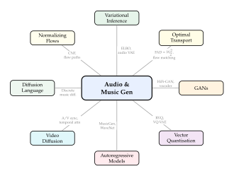
Remark 70 (The breadth of connections).
The connections enumerated above are not merely analogies; they represent shared mathematical structures. The ELBO, optimal transport distances, adversarial training, vector quantisation, autoregressive factorisation, and discrete diffusion are all instantiations of general frameworks that manifest differently in the audio domain due to the specific properties of audio signals (high dimensionality, strong temporal structure, perceptual sensitivity to phase and periodicity). Understanding these connections enables practitioners to transfer insights across modalities: an advance in image VAE training may improve audio autoencoders, a faster ODE solver for video diffusion may accelerate audio latent diffusion, and a better quantisation scheme for language models may yield better audio codecs.
Open Problems and Future Directions
Despite the remarkable progress documented in this chapter, audio and music generation systems remain far from the ideal creative tool. In this section, we identify five fundamental open problems that define the frontier of the field. For each problem, we provide a formal statement, discuss why it is hard, and outline promising directions of attack.
Real-Time Interactive Generation
Throughput is no longer the obstacle. The systems surveyed in this chapter generate audio comfortably faster than real time on a modern GPU: the codec pipeline of Example 9 runs at RTF , Stable Audio produces 45 seconds of music in 2.5 seconds (Example 18), few-step flow matching reaches RTF (tab:audiogen:nfe-wallclock), distilled consistency models RTF (Example 23), and chunked long-form generation RTF over three minutes (Example 26).
What remains hard is latency, which is a different quantity. Real-time factor measures total wall-clock time divided by output duration and can be driven down by batching and by generating a long clip in one shot; interactive use instead requires that the first sample appear within tens of milliseconds of the triggering event, and that every subsequent block arrive before its playout deadline, with no batching over the future and no opportunity to look ahead. A model that generates 30 seconds of audio in 0.5 seconds has an excellent RTF and a 500 ms latency, which is an order of magnitude too slow for a musician playing an instrument. Interactive applications (live performance, game audio, conversational agents) are bounded by the second number, not the first.
Problem 1 (Real-Time Audio Generation).
Design a generative audio model that produces audio of quality comparable to current state-of-the-art systems while satisfying the following latency constraints:
Conversational speech: end-to-end latency (from text input to first audio sample) below ms.
Interactive music: latency from control signal change (e.g., a key press, a tempo change) to audible response below ms.
Sound effects: latency from trigger event to onset below ms (the threshold for perceived synchronisation in audiovisual media).
The total computational budget must fit within a single consumer GPU or (ideally) a mobile device's neural processing unit.
The latency budget can be decomposed into three stages, each of which must be optimised.
Encoding stage: Computing the conditioning representation (text embedding, control signal processing). This is typically fast ( ms) and is not the bottleneck.
Generation stage: Running the diffusion or autoregressive model to produce the latent representation. For a diffusion model with denoising steps, each requiring a full forward pass through a large transformer, this is the dominant cost. Consistency distillation (reducing to 1–4 steps) and model distillation (reducing the model size) are the principal approaches.
Decoding stage: Converting the latent representation to a waveform via the decoder/vocoder. For a streaming codec decoder, this can operate in real-time with modest computation, but the latency depends on the codec's frame size.
Remark 71 (Streaming generation).
Real-time generation requires a streaming architecture that can begin outputting audio before the entire generation is complete. For autoregressive models (MusicGen, VALL-E), streaming is natural: each token can be decoded and output as soon as it is generated. For diffusion models, streaming is more challenging because the standard denoising process operates on the entire latent simultaneously. Promising approaches include chunked diffusion (generating overlapping segments and crossfading) and causal diffusion architectures that denoise from left to right.
Song-Length Coherence
Duration alone is no longer the barrier: as tab:audiogen:commercial-comparison records, Suno and Udio already emit four-minute tracks, and research systems reach 95 seconds in a single shot. What is still missing is structure over those durations. Open research models generate 10 to 30 seconds before their context window runs out, and the commercial systems that go further do so by chunking or by planning at a coarse resolution, which buys length but not guaranteed thematic return. Generating a complete song (3 to 5 minutes) whose verses, choruses, bridge, key changes and dynamic arc are genuinely related to one another - rather than locally plausible and globally arbitrary - remains an open problem.
Problem 2 (Song-Length Musical Coherence).
Generate a piece of music of duration seconds (3 minutes) that satisfies:
Local quality: Every 5-second segment, evaluated in isolation, is indistinguishable from a human-composed recording.
Structural coherence: The piece exhibits recognisable musical form (e.g., AABA, verse-chorus) with thematic recurrence: melodic motifs introduced in the first 30 seconds reappear (possibly varied) later in the piece.
Harmonic consistency: The piece maintains a coherent key centre (with possible modulations) and avoids unintended harmonic discontinuities.
Dynamic arc: The piece has a perceptible narrative in terms of energy, texture, and instrumentation that builds, peaks, and resolves.
The difficulty lies in the mismatch between the model's context window and the time scales of musical structure. A typical diffusion model's context window covers 10–30 seconds, but musical structure operates at multiple hierarchical levels:
| Level | Time scale | Examples |
| Sample/grain | ms | Timbre, onset transient |
| Beat/note | 100–500 ms | Rhythm, melody |
| Phrase | 2–8 s | Melodic phrase, chord progression |
| Section | 15–60 s | Verse, chorus, bridge |
| Song | 3–5 min | Overall form, dynamic arc |
Remark 72 (Analogy to long video).
The song-coherence problem is the audio analogue of the long video generation problem discussed in 20. Both require maintaining global structure over time spans that far exceed the model's native context window. Autoregressive chunk generation, hierarchical planning, and global conditioning signals (e.g., a structural outline) are promising shared strategies.
Faithful Instrument and Vocal Rendering
Even the best current systems produce audio that experts can distinguish from real recordings. The gap is most apparent for solo instruments and vocals, where listeners have extremely sensitive expectations.
Conjecture 3 (Codec Bottleneck Hypothesis).
As neural audio codec quality approaches perceptual transparency, the quality bottleneck in generated audio shifts from the codec to the generative model. (For neural codecs this chapter puts that threshold at roughly 6 kbps for near-transparency and 12 kbps for transparency; see tab:audiogen:encodec-bitrates and Example 6. The familiar figure of approximately 128 kbps belongs to the transform codecs, MP3 and AAC, and is about twenty times higher - which is the point of neural codecs, and not a threshold that applies to them.) Formally, let denote the codec reconstruction error and denote the generation error (measured as the gap between the generated and real distributions in the latent space). We conjecture that there exists a codec quality threshold such that (Codec Bottleneck) where is a monotonically increasing function independent of the codec. Beyond this threshold, improving the codec yields diminishing returns; the dominant source of artifacts is the generative model's inability to capture the full complexity of the audio distribution.
This conjecture, if true, implies that future progress in audio generation quality requires advances in the generative model itself (better architectures, training procedures, and data) rather than better audio compression.
Remark 73 (Perceptual evaluation frontier).
The gap between generated and real audio is most reliably measured by trained listeners (MOS scores), but even human evaluation has limitations: judgements depend on the listening environment, familiarity with the instrument, and the evaluator's musical training. For solo piano, expert listeners can detect subtle timing irregularities of less than 5 ms and pitch deviations of less than 5 cents. Achieving imperceptible generation for such demanding material requires the generative model to capture the full joint distribution over pitch, timing, dynamics, and timbre at resolutions that approach the limits of human perception.
Unified Audio Generation
Current systems are specialised: separate models for speech synthesis, music generation, and sound effect production. A unified model that handles all audio modalities with a single architecture and a single set of weights would be both more efficient and more capable, enabling cross-modal generation (e.g., generating music with lyrics, or sound effects synchronised to speech).
Problem 3 (Unified Audio Generation).
Design a single generative model over the space of all audio signals conditioned on a multimodal prompt (text, audio, MIDI, video, etc.) such that:
Speech quality: The model generates speech at quality matching or exceeding specialised TTS systems, with accurate prosody, emotion, and speaker identity.
Music quality: The model generates music at quality matching or exceeding specialised music generation systems, with faithful instrumentation and musical structure.
Sound effect quality: The model generates environmental sounds, Foley effects, and mechanical sounds with physical plausibility.
Compositional generation: The model can generate mixtures (speech over background music, music with sound effects) with appropriate relative levels and temporal alignment.
The principal challenge is the distributional diversity: speech, music, and sound effects have very different statistical properties (spectral envelopes, temporal dynamics, harmonic structures). A single model must learn to represent all of these within a shared latent space without sacrificing quality in any modality.
Remark 74 (Connection to multimodal video generation).
The unified audio generation problem is a component of the broader unified multimodal generation problem discussed in 20. A system that can generate video with synchronised audio, speech, music, and sound effects would subsume both the video and audio generation challenges.
Verifiable Provenance
As discussed in Detection and Watermarking, current watermarking systems face a fundamental tension between robustness and imperceptibility, bounded by the information-theoretic capacity of the watermarking channel (Proposition 47).
Problem 4 (Robust Unforgeable Audio Watermarking).
Design a watermarking system that embeds a payload in audio signals with the following properties:
Imperceptibility: The watermarked signal is perceptually indistinguishable from the original (PESQ degradation , ViSQOL degradation ).
Robustness: The payload is recoverable after any combination of the attacks in Remark 65 with bit error rate .
Unforgeability: It is computationally infeasible (under standard cryptographic assumptions) for an adversary without the embedding key to produce audio that the decoder classifies as watermarked.
Capacity: The payload length bits, sufficient to encode a unique identifier for the generating system and a timestamp.
The system must operate in real-time (embedding and detection each require ms per second of audio).
The unforgeability requirement connects to the cryptographic literature on digital signatures and commitment schemes. The challenge is that unlike traditional digital signatures (which protect a specific bitstring), audio watermarks must survive signal-processing transformations that alter the audio content while preserving its perceptual identity.
Key Idea.
The provenance frontier. Solving the verifiable provenance problem requires bridging information theory (capacity bounds), signal processing (robustness to transformations), perceptual science (imperceptibility), and cryptography (unforgeability). No existing system satisfies all four requirements simultaneously. Progress on this problem is essential for building a trustworthy audio ecosystem in which the provenance of every audio signal can be verified.
Exercises
Exercise 23 (STFT and Mel Spectrogram Frame Count).
Consider an audio signal sampled at rate (samples per second). The Short-Time Fourier Transform (STFT) is computed with a window of length samples and a hop size of samples. A mel filterbank with triangular filters is applied to the magnitude STFT to produce the mel spectrogram .
Show that the number of STFT frames is (Frame Count) Hint: The -th frame is centred at sample (for ), and the last valid frame must have its window entirely within the signal.
For an audio signal of duration seconds at sample rate Hz, window length , and hop size , compute the number of frames as a function of . What is for s?
The mel spectrogram has shape . For mel bins, compute the total number of real-valued entries in the mel spectrogram for s. Compare this to the number of samples in the original waveform. What is the compression ratio?
The frequency resolution of the STFT is and the time resolution is . Show that their product satisfies the uncertainty principle: (Uncertainty) with equality when (no overlap). Explain the trade-off between time and frequency resolution.
The mel scale is approximately linear below 1 kHz and logarithmic above 1 kHz. Using the definition (where is in Hz and is in mels), compute the mel values at Hz and Hz. Verify that the interval from 1 kHz to 8 kHz, a factor of in Hz, corresponds to a substantially smaller ratio in mel space, and give that ratio to two decimal places. (You should find and , a ratio of about : compression by roughly , not the near-total flattening sometimes claimed. Then explain why the compression is so much milder than the word “logarithmic” suggests, by examining the offset in the formula.)
Exercise 24 (RVQ Approximation Error Bound).
Consider a residual vector quantiser (RVQ) with stages, each using a codebook of vectors in . Let be a latent vector to be quantised.
Define the RVQ encoding recursively: , and for , (RVQ Recursive) Show that the reconstruction is and the quantisation error is .
Suppose each codebook is “well-distributed” in the sense that for any vector with , there exists a codebook vector satisfying for a contraction factor . Prove that the RVQ quantisation error satisfies (RVQ Error Bound) Hint: Show by induction that . Note that this is a different hypothesis from the one used in Theorem 1, which assumes a per-stage energy gain and yields ; the two agree when at every stage. State which of the two hypotheses a trained codebook is more likely to satisfy, and why.
Note first that the hypothesis of part (b) cannot be met by a codebook of fixed unit vectors: a relative bound must hold for residuals of every magnitude, and a fixed codebook fails it as soon as is small. Assume instead the normalised form used by DAC: the residual direction is quantised to the nearest of unit vectors and rescaled by , so is the covering radius of the codebook on the sphere . Show, by a volume (covering-number) argument, that covering to accuracy requires , hence (RVQ Covering) Conclude that driving down by a constant factor costs a factor in codebook size, so a single codebook is hopeless in high dimensions. Explain how stacking stages evades this: it buys error at bits, i.e. error exponential in the bit budget, whereas a single codebook of the same total size buys only .
Compare the total number of bits used by RVQ ( bits per vector) with scalar quantisation ( bits per vector, where is the number of bits per dimension). For what range of does RVQ use fewer bits for the same reconstruction error?
In practice, RVQ codebooks are trained jointly with the encoder and decoder using the straight-through estimator. Explain why the gradient cannot be computed exactly through the operation, and describe how the straight-through estimator approximates it.
Exercise 25 (Codebook Pattern Complexity).
Consider a neural audio codec with codebook levels producing tokens per second. For a clip of duration seconds, the total number of tokens per codebook is .
Flattened pattern. All tokens are arranged in a single sequence in raster order (all codebooks for time step 1, then all codebooks for time step 2, etc.). The sequence length is . For an autoregressive transformer with dimensions, the self-attention cost per layer is . Express this in terms of , , and .
Delay pattern. Codebook is delayed by time steps. At each step, the model predicts one token per codebook, but codebook uses context from time step . The effective sequence length is . Show that the attention cost per layer is and compare to the flattened pattern. Note: there is no extra factor of here. As in the parallel pattern, the tokens of a position are summed into a single -dimensional embedding before the transformer sees them, and the model runs one attention computation over positions, not of them. The appears only in the input embedding and output head costs, both linear in the sequence length.
Parallel pattern. All codebooks at the same time step are predicted simultaneously (in parallel). The sequence length is . The model uses a single transformer forward pass per time step to predict tokens. Show that the attention cost per layer is , independent of . What is the trade-off in terms of modelling quality?
For , tokens/second, s, and , compute the attention cost (in units of multiplications) for each of the three patterns. Which pattern is most efficient? By what factor?
Discuss the quality-efficiency trade-off: the flattened pattern models all dependencies but is slowest; the parallel pattern is fastest but loses inter-codebook dependencies at the same time step. The delay pattern is a compromise. Under what assumptions about the statistical structure of codec tokens is the parallel pattern a good approximation?
Exercise 26 (OT Conditional Path for Audio Latents).
Consider a flow matching framework for audio latent diffusion. Let be a clean audio latent and be Gaussian noise. The optimal transport (OT) conditional path is defined as (OT PATH)
Compute the conditional velocity field and show that it is constant in : (Const Velocity)
Show that the conditional path has constant speed: for all . Interpret this geometrically: each sample travels along a straight line from data to noise at uniform speed.
The flow matching training loss is (FM LOSS) where , , , and . Setting , eliminate to obtain , and deduce that the flow-matching loss is the denoising score matching loss with a -dependent weight: (FM DSM) where is the induced noise predictor. Conclude that the two objectives have the same minimiser but are not equal up to an additive or multiplicative constant: the weight diverges as , so flow matching places far more emphasis on the high-noise end of the schedule than an unweighted DDPM loss does. Discuss what this implies for audio, where the low-noise steps carry the fine spectral detail.
At inference time, generation proceeds by solving the ODE from (noise) to (data). Using the Euler method with steps (step size ), write the update rule and show that the total number of model evaluations is exactly .
For audio applications, the latent encodes a mel spectrogram of shape (flattened to with ). The straightness of the OT path means that Euler integration with few steps ( to ) produces high-quality results. Explain why this is particularly advantageous for audio, where generation speed directly impacts usability.
Exercise 27 (Consistency Distillation for Audio Diffusion).
Let follow the probability flow ODE of an audio diffusion model: (PF ODE) where are the drift and diffusion coefficients of the forward SDE and (Sigma T) is the noise standard deviation, and is the pretrained teacher denoiser. (Check the sign in (Sigma T) against the variance-preserving choice with : the exponent must be negative for to be real and to increase from towards . Writing instead makes the radicand negative for every .) To avoid a collision with the drift coefficient , the consistency function is written below.
A consistency function maps any point on a PF-ODE trajectory to its origin . State the self-consistency property: for any with , provided and lie on the same ODE trajectory.
The consistency distillation loss is (CD LOSS) where are adjacent time steps in a discretisation , is obtained by one ODE step from using the teacher, is the EMA of , and is a distance function (e.g., or LPIPS). Derive the gradient and explain why the EMA target prevents collapse.
After distillation, one-step generation produces from . The quality gap relative to the multi-step teacher depends on how well the consistency property is satisfied. Take , so that is a mean squared distance, and suppose the teacher's own discretisation error is negligible. Show that if , then with the number of steps and , (CD Quality) Hint: telescope over the consecutive pairs, apply the triangle inequality, and then use on each term (Jensen). Explain why the square root is unavoidable here: a bound on a mean squared distance controls a mean distance only through its square root, so quoting silently assumes is already a norm.
AudioLCM applies consistency distillation to an audio latent diffusion model (e.g., AudioLDM2). The key challenge is that the teacher's denoiser is a large U-Net operating on mel spectrogram latents. Discuss how the choice of distance function affects the quality of the distilled model. Why might a perceptual distance (e.g., multi-scale STFT loss) be preferable to distance for audio?
Exercise 28 (FAD as Squared Wasserstein Distance).
The Fréchet Audio Distance (FAD) between two sets of audio clips is defined analogously to FID: (FAD DEF) where and are the means and covariances of features extracted from real and generated audio by a pretrained VGGish network.
Recall from 14 that the squared -Wasserstein distance between two Gaussians and on is given by the Dowson–Landau–Olkin–Pukelsheim formula: (W2 Gaussian) Show that . Hint: Use the cyclic property of the trace and the fact that and have the same eigenvalues.
Using part (a), conclude that .
Show that if and only if and . Hint: For the “if” direction, substitute directly. For the “only if” direction, note that , so FAD implies . Then show that implies by considering the eigenvalues of .
Compute the FAD between two univariate Gaussians and . Verify that it simplifies to .
Exercise 29 (Information-Theoretic Watermark Capacity).
Consider an audio watermarking system that embeds bits into a host signal . The watermarked signal is , where is the watermark perturbation subject to a power constraint . The channel applies an attack , producing , where is additive noise with power .
Modelling the watermarking system as a communication channel with input and output (assuming the host is known at both encoder and decoder as “side information”), show that the channel reduces to a standard additive white Gaussian noise (AWGN) channel with input power and noise power .
Apply Shannon's channel coding theorem to bound the maximum payload: (Capacity)
The imperceptibility constraint requires for a perceptual distortion budget . For (watermark amplitude at most 1% of signal amplitude), (SNR of 30 dB attack noise), and (one second at 16 kHz), compute the maximum payload .
In the rate-distortion framework, increasing the payload requires either increasing (more distortion) or decreasing (weaker attack). Plot the Pareto frontier in the plane for fixed and . At what value of can we embed exactly bits?
Discuss why practical watermarking systems achieve payloads well below the Shannon limit. Identify at least three factors that reduce the effective capacity (non-Gaussianity of the host, non-AWGN attacks, perceptual constraints that are more restrictive than a power constraint).
Exercise 30 (Bayesian Source Separation).
Consider an observed audio mixture , where are independent source signals (e.g., vocals, drums, bass, other). Each source has a prior distribution learned by a diffusion model with score function .
Write the posterior distribution over sources given the mixture: (Posterior) where is the Dirac delta enforcing the mixture constraint.
By introducing a relaxed mixture constraint , show that the score function for the relaxed posterior with respect to source is (SEP Score)
Describe how to use Langevin dynamics with the score in part (b) to sample from the posterior, obtaining separated sources. Write the update rule for source at iteration : (Langevin SEP) where .
In the limit , the relaxed constraint becomes exact. Explain why taking too small causes numerical instability, and discuss strategies for annealing during sampling.
This approach requires running diffusion models simultaneously (one per source). For sources and a diffusion model with denoising steps, compute the total number of neural network forward passes. Compare to a direct separation model (a single forward pass that outputs all sources).
Exercise 31 (Beat-Synchronous Mixup).
Beat-synchronous mixup is a data augmentation strategy for music generation models. Given two music clips and with beat positions and , the augmented clip is formed by alternating segments from each clip at beat boundaries.
Formalise beat-synchronous mixup. Define the augmented clip by selecting, at each beat position, whether to use a segment from or according to independent Bernoulli coin flips : (BEAT Mixup)
Show that the marginal distribution of beat positions in is preserved. Specifically, let denote the inter-beat interval. If both clips have the same tempo (so that for all ), show that the distribution of inter-beat intervals in is identical to that in either original clip.
The mixup operation introduces discontinuities at beat boundaries where the source switches. In the STFT domain, these discontinuities appear as broadband transients. Argue that crossfading over a window of samples (typically at 22 kHz, corresponding to ms) eliminates perceptible clicks while preserving the beat structure, provided for all .
Show that for , the expected fraction of that comes from is , and the probability that any given beat segment comes from is independent of all other segments.
Discuss the benefit of beat-synchronous mixup for training music generation models. How does it increase the effective diversity of the training set? What musical properties are preserved, and what properties are disrupted?
Exercise 32 (CFG for Audio Diffusion).
Let be an audio diffusion denoiser conditioned on a text prompt embedding , trained with classifier-free guidance by randomly dropping the conditioning with probability .
Write the CFG-modified noise prediction: (CFG) where is the guidance scale and denotes the null (unconditional) embedding. Show that this is equivalent to .
Interpret CFG in terms of the score function. Recall that . Show that the guided score is (CFG Score) This is the score of the distribution , which sharpens the conditional distribution.
For audio generation, the guidance scale affects the spectral characteristics of the output. At high (e.g., ), the generated audio tends to have exaggerated spectral peaks (louder harmonics, sharper formants) and reduced spectral diversity. Explain this phenomenon by analysing the effect of the exponent on the conditional distribution: large concentrates probability mass on the modes of , producing outputs that are maximally “on-topic” but less diverse.
In practice, to is typical for text-to-audio generation. Quantify the price of that amplification. Write the two network outputs as and , where denotes the exact conditional and unconditional noise and the model's estimation error, with , and correlation coefficient . Show that the estimation error of the guided prediction has second moment (CFG Noise) Evaluate this at for two regimes: perfectly correlated errors (, ), where it collapses to because the shared error cancels; and independent errors (), where it is , an amplification of the error standard deviation by . Explain why the conditional and unconditional branches of a single network with a dropped-condition token tend towards the first regime, and why this - not any change in “denoising efficiency” - is what makes large guidance scales usable at all.
Propose and justify a frequency-dependent guidance strategy: use a higher guidance scale for low frequencies (below 1 kHz, where pitch and harmony are determined) and a lower scale for high frequencies (above 4 kHz, where timbre and noise reside). Write the modified CFG formula and explain why this might produce more natural-sounding audio.
Exercise 33 (Timing Conditioning and Variable-Length Generation).
Stable Audio and similar systems condition the diffusion model on
a pair of timing scalars. Following
Definition 36, and matching the real system's
seconds_start / seconds_total pair, we take the
pair to be : the start time of the desired
segment within a longer piece, and the total duration of
that piece. (Some presentations write instead; the two parameterisations are
interchangeable, but they are not the same variables, and mixing
them is a common source of confusion.)
The timing-conditioned diffusion model learns , where is the text prompt. Show that the marginal over all valid timing pairs gives the distribution over variable-length audio: (Timing Marginal) This is a direct application of the law of total probability.
In practice, at inference time one sets specific values , for a desired duration . Explain how this enables generating audio of any duration at test time, even if the model was trained on clips of varying lengths.
The timing values are encoded as sinusoidal positional embeddings (analogous to those used in transformers). For a single timing value , the embedding is , where are geometrically spaced frequencies and is the number of frequency bands (not to be confused with the duration above). Show that the inner product depends only on , making the embedding translation-equivariant.
Derive the inner product explicitly: (Timing Inner) Hint: Use the identity .
If is much larger than the training set's maximum duration, the model is asked to extrapolate to unseen timing values. Discuss why sinusoidal embeddings enable moderate extrapolation (the inner product kernel is smooth and periodic) but fail for very large extrapolation (the model has never seen the corresponding timing values during training).
Exercise 34 (Snake Activation Function).
The Snake activation function, used in audio neural networks (BigVGAN, DAC), is defined as (Snake DEF) where is a learnable parameter controlling the frequency of the periodic component.
Show that is monotonically increasing for all . To do this, compute the derivative: (Snake Deriv) Then show that for all , with equality only at isolated points.
Since with equality at for , the derivative satisfies for all . Conclude that is non-decreasing, and argue that it is strictly increasing (i.e., the zero-derivative points are isolated and do not form intervals).
Show that as , , so that Snake reduces to the identity plus a quadratic term. Hint: Use the Taylor expansion .
Show that as , in the time-averaged sense: the oscillatory term averages to over any interval of length . Thus, for large , Snake behaves approximately like the identity with a small positive bias.
Explain why the periodic component of Snake is particularly well-suited for audio neural networks. The parameter can learn to match the fundamental frequency of the audio being modelled, enabling the network to represent periodic waveforms with fewer parameters than non-periodic activations (ReLU, GELU). Compute the Fourier series of exactly. Hint: write and apply the Jacobi–Anger expansion , where is the Bessel function of the first kind. You should obtain (Snake Fourier) i.e. a DC offset, the fundamental at with its amplitude unchanged, and even harmonics at with amplitudes . All odd harmonics above the fundamental vanish, because is an even function of its argument. Verify numerically at , that the harmonic amplitudes are at , then at through . Finally, note why the frequencies “” sometimes quoted for this expansion cannot be right: has units of inverse amplitude and of radians per second, so the two cannot be added. The product is dimensionless, and it is a Bessel argument - it controls how much harmonic energy appears, not where the harmonics sit.
References
-
BigVGAN: A Universal Neural Vocoder with Large-Scale Training
BibTeX
@inproceedings{lee2023bigvgan, title={{BigVGAN}: A Universal Neural Vocoder with Large-Scale Training}, author={Lee, Sang-gil and Ping, Wei and Ginsburg, Boris and Catanzaro, Bryan and Yoon, Sungroh}, booktitle={International Conference on Learning Representations}, year={2023} }Conference paper
-
Signal Estimation from Modified Short-Time Fourier Transform
BibTeX
@article{griffin1984signal, title={Signal Estimation from Modified Short-Time {Fourier} Transform}, author={Griffin, Daniel and Lim, Jae}, journal={IEEE Transactions on Acoustics, Speech, and Signal Processing}, volume={32}, number={2}, pages={236--243}, year={1984}, publisher={IEEE} }Journal article
-
Online and Linear-Time Attention by Enforcing Monotonic Alignments
BibTeX
@inproceedings{raffel2017online, title={Online and Linear-Time Attention by Enforcing Monotonic Alignments}, author={Raffel, Colin and Luong, Minh-Thang and Liu, Peter J and Weiss, Ron J and Eck, Douglas}, booktitle={International Conference on Machine Learning}, pages={2837--2846}, year={2017} }Conference paper
-
RePaint: Inpainting using Denoising Diffusion Probabilistic Models
BibTeX
@inproceedings{lugmayr2022repaint, title={{RePaint}: Inpainting using Denoising Diffusion Probabilistic Models}, author={Lugmayr, Andreas and Danelljan, Martin and Romero, Andres and Yu, Fisher and Timofte, Radu and Van Gool, Luc}, booktitle={IEEE/CVF Conference on Computer Vision and Pattern Recognition}, pages={11461--11471}, year={2022} }Conference paper
-
Pop Music Transformer: Beat-based Modeling and Generation of Expressive Pop Piano Compositions
BibTeX
@inproceedings{huang2020pop, title={Pop Music Transformer: Beat-based Modeling and Generation of Expressive Pop Piano Compositions}, author={Huang, Yu-Siang and Yang, Yi-Hsuan}, booktitle={Proceedings of the 28th ACM International Conference on Multimedia}, pages={1180--1188}, year={2020} }Conference paper
-
Compound Word Transformer: Learning to Compose Full-Song Music over Dynamic Directed Hypergraphs
BibTeX
@inproceedings{hsiao2021compound, title={Compound Word Transformer: Learning to Compose Full-Song Music over Dynamic Directed Hypergraphs}, author={Hsiao, Wen-Yi and Liu, Jen-Yu and Yeh, Yin-Cheng and Yang, Yi-Hsuan}, booktitle={Proceedings of the AAAI Conference on Artificial Intelligence}, volume={35}, number={1}, pages={178--186}, year={2021} }Conference paper
-
MusicBERT: Symbolic Music Understanding with Large-Scale Pre-Training
BibTeX
@inproceedings{zeng2021musicbert, title={{MusicBERT}: Symbolic Music Understanding with Large-Scale Pre-Training}, author={Zeng, Mingliang and Tan, Xu and Wang, Rui and Ju, Zeqian and Qin, Tao and Liu, Tie-Yan}, booktitle={Findings of the Association for Computational Linguistics: ACL-IJCNLP 2021}, pages={791--800}, year={2021} }Conference paper
-
Structured denoising diffusion models in discrete state-spaces
BibTeX
@article{austin2021structured, title={Structured denoising diffusion models in discrete state-spaces}, author={Austin, Jacob and Johnson, Daniel D and Ho, Jonathan and Tarlow, Daniel and van den Berg, Rianne}, journal={Advances in Neural Information Processing Systems}, volume={34}, pages={17981--17993}, year={2021} }Journal article
-
MuLan: A Joint Embedding of Music Audio and Natural Language
BibTeX
@article{huang2022mulan, title={{MuLan}: A Joint Embedding of Music Audio and Natural Language}, author={Huang, Qingqing and Jansen, Aren and Lee, Heiga and Ganti, Ravi and Li, Judith Yue and Ellis, Daniel P W}, journal={arXiv preprint arXiv:2208.12415}, year={2022} }Journal article
-
SoundStream: An End-to-End Neural Audio Codec
BibTeX
@article{zeghidour2021soundstream, title={{SoundStream}: An End-to-End Neural Audio Codec}, author={Zeghidour, Neil and Luebs, Alejandro and Omran, Ahmed and Skoglund, Jan and Tagliasacchi, Marco}, journal={IEEE/ACM Transactions on Audio, Speech, and Language Processing}, volume={30}, pages={495--507}, year={2021} }Journal article
-
CNN Architectures for Large-Scale Audio Classification
BibTeX
@inproceedings{hershey2017cnn, title={{CNN} Architectures for Large-Scale Audio Classification}, author={Hershey, Shawn and Chaudhuri, Sourish and Ellis, Daniel P W and Gemmeke, Jort F and Jansen, Aren and Moore, R Channing and Plakal, Manoj and Platt, Devin and Sauber, Rif A and Seybold, Bryan and others}, booktitle={IEEE International Conference on Acoustics, Speech and Signal Processing (ICASSP)}, pages={131--135}, year={2017}, organization={IEEE} }Conference paper
-
ViSQOL: An Objective Speech Quality Model
BibTeX
@article{hines2015visqol, title={{ViSQOL}: An Objective Speech Quality Model}, author={Hines, Andrew and Skoglund, Jan and Kokaram, Anil C. and Harte, Naomi}, journal={EURASIP Journal on Audio, Speech, and Music Processing}, year={2015} }Journal article
-
WaveNet: A Generative Model for Raw Audio
BibTeX
@article{oord2016wavenet, author = {van den Oord, Aaron and Dieleman, Sander and Zen, Heiga and Simonyan, Karen and Vinyals, Oriol and Graves, Alex and Kalchbrenner, Nal and Senior, Andrew and Kavukcuoglu, Koray}, title = {{WaveNet}: A Generative Model for Raw Audio}, journal = {arXiv preprint arXiv:1609.03499}, year = {2016} }Journal article
-
Parallel WaveNet: Fast High-Fidelity Speech Synthesis
BibTeX
@article{oord2018parallel, title={Parallel {WaveNet}: Fast High-Fidelity Speech Synthesis}, author={van den Oord, A{\"a}ron and Li, Yazhe and Babuschkin, Igor and Simonyan, Karen and Vinyals, Oriol and Kavukcuoglu, Koray and van den Driessche, George and Lockhart, Edward and Cobo, Luis C and Stimberg, Florian and others}, journal={arXiv preprint arXiv:1711.10433}, year={2018} }Journal article
-
Efficient Neural Audio Synthesis
BibTeX
@article{kalchbrenner2018efficient, title={Efficient Neural Audio Synthesis}, author={Kalchbrenner, Nal and Elsen, Erich and Simonyan, Karen and Noury, Seb and Casagrande, Norman and Lockhart, Edward and Stimberg, Florian and Oord, A{\"a}ron van den and Dieleman, Sander and Kavukcuoglu, Koray}, journal={arXiv preprint arXiv:1802.08435}, year={2018} }Journal article
-
MelGAN: Generative Adversarial Networks for Conditional Waveform Synthesis
BibTeX
@inproceedings{kumar2019melgan, title={{MelGAN}: Generative Adversarial Networks for Conditional Waveform Synthesis}, author={Kumar, Kundan and Kumar, Rithesh and de Boissiere, Thibault and Gestin, Lucas and Teoh, Wei Zhen and Sotelo, Jose and de Br{\'e}bisson, Alexandre and Bengio, Yoshua and Courville, Aaron C.}, booktitle={Advances in Neural Information Processing Systems}, year={2019} }Conference paper
-
HiFi-GAN: Generative Adversarial Networks for Efficient and High Fidelity Speech Synthesis
BibTeX
@inproceedings{kong2020hifi, title={{HiFi-GAN}: Generative Adversarial Networks for Efficient and High Fidelity Speech Synthesis}, author={Kong, Jungil and Kim, Jaehyeon and Bae, Jaekyoung}, booktitle={Advances in Neural Information Processing Systems}, volume={33}, pages={17022--17033}, year={2020} }Conference paper
-
UnivNet: A Neural Vocoder with Multi-Resolution Spectrogram Discriminators for High-Fidelity Waveform Generation
BibTeX
@inproceedings{jang2021univnet, title={{UnivNet}: A Neural Vocoder with Multi-Resolution Spectrogram Discriminators for High-Fidelity Waveform Generation}, author={Jang, Won and Lim, Dan and Yoon, Jaesam and Kim, Bjoern and Kim, Juntae}, booktitle={Interspeech}, pages={2207--2211}, year={2021} }Conference paper
-
DiffWave: A Versatile Diffusion Model for Audio Synthesis
BibTeX
@inproceedings{kong2021diffwave, title={{DiffWave}: A Versatile Diffusion Model for Audio Synthesis}, author={Kong, Zhifeng and Ping, Wei and Huang, Jiaji and Zhao, Kexin and Catanzaro, Bryan}, booktitle={International Conference on Learning Representations}, year={2021} }Conference paper
-
WaveGrad: Estimating Gradients for Waveform Generation
BibTeX
@article{chen2020wavegrad, title={{WaveGrad}: Estimating Gradients for Waveform Generation}, author={Chen, Nanxin and Zhang, Yu and Zen, Heiga and Weiss, Ron J and Norouzi, Mohammad and Chan, William}, journal={arXiv preprint arXiv:2009.00713}, year={2020} }Journal article
-
AudioLDM: Text-to-Audio Generation with Latent Diffusion Models
BibTeX
@inproceedings{liu2023audioldm, title={{AudioLDM}: Text-to-Audio Generation with Latent Diffusion Models}, author={Liu, Haohe and Chen, Zehua and Yuan, Yi and Mei, Xinhao and Liu, Xubo and Mandic, Danilo and Wang, Wenwu and Plumbley, Mark D.}, booktitle={International Conference on Machine Learning}, year={2023} }Conference paper
-
Simple and Controllable Music Generation
BibTeX
@article{copet2024simple, title={Simple and Controllable Music Generation}, author={Copet, Jade and Kreuk, Felix and Gat, Itai and Remez, Tal and Kant, David and Synnaeve, Gabriel and Adi, Yossi and D{\'e}fossez, Alexandre}, journal={Advances in Neural Information Processing Systems}, volume={36}, year={2024} }Journal article
-
Long-Form Music Generation with Latent Diffusion
BibTeX
@article{evans2024stable, title={Long-Form Music Generation with Latent Diffusion}, author={Evans, Zach and Parker, Julian D. and Carr, CJ and Zukowski, Zack and Taylor, Josiah and Pons, Jordi}, journal={arXiv preprint arXiv:2404.10301}, year={2024} }Journal article
-
High Fidelity Neural Audio Compression
BibTeX
@article{defossez2022high, title={High Fidelity Neural Audio Compression}, author={D{\'e}fossez, Alexandre and Copet, Jade and Synnaeve, Gabriel and Adi, Yossi}, journal={arXiv preprint arXiv:2210.13438}, year={2022} }Journal article
-
High-Fidelity Audio Compression with Improved RVQGAN
BibTeX
@article{kumar2024high, title={High-Fidelity Audio Compression with Improved {RVQGAN}}, author={Kumar, Rithesh and Seetharaman, Prem and Luebs, Alejandro and Kumar, Ishaan and Kumar, Kundan}, journal={Advances in Neural Information Processing Systems}, volume={36}, year={2024} }Journal article
-
Diff-BGM: A Diffusion Model for Video Background Music Generation
BibTeX
@article{li2024diffbgm, title={{Diff-BGM}: A Diffusion Model for Video Background Music Generation}, author={Li, Sizhe and Qin, Yiming and Zheng, Minghang and Jin, Xin and Liu, Yang}, journal={Conference on Computer Vision and Pattern Recognition}, year={2024} }Journal article
-
VidMuse: A Simple Video-to-Music Generation Framework with Long-Short-Term Modeling
BibTeX
@article{tian2024vidmuse, title={{VidMuse}: A Simple Video-to-Music Generation Framework with Long-Short-Term Modeling}, author={Tian, Zeyue and Liu, Zhaoyang and Yuan, Ruibin and Pan, Jiahao and Liu, Qifeng and Tan, Xu and Chen, Qifeng and Xue, Wei and Guo, Yike}, journal={Conference on Computer Vision and Pattern Recognition}, year={2025} }Journal article
-
Jukebox: A Generative Model for Music
BibTeX
@article{dhariwal2020jukebox, title={Jukebox: A Generative Model for Music}, author={Dhariwal, Prafulla and Jun, Heewoo and Payne, Christine and Kim, Jong Wook and Radford, Alec and Sutskever, Ilya}, journal={arXiv preprint arXiv:2005.00341}, year={2020} }Journal article
-
Music Transformer: Generating Music with Long-Term Structure
BibTeX
@inproceedings{huang2019music, title={Music Transformer: Generating Music with Long-Term Structure}, author={Huang, Cheng-Zhi Anna and Vaswani, Ashish and Uszkoreit, Jakob and Shazeer, Noam and Simon, Ian and Hawthorne, Curtis and Dai, Andrew M and Hoffman, Matthew D and Dinculescu, Monica and Eck, Douglas}, booktitle={International Conference on Learning Representations}, year={2019} }Conference paper
-
MusicLM: Generating Music From Text
BibTeX
@article{agostinelli2023musiclm, title={{MusicLM}: Generating Music From Text}, author={Agostinelli, Andrea and Denk, Timo I. and Borsos, Zal{\'a}n and Engel, Jesse and Verzetti, Mauro and Caillon, Antoine and Huang, Qingqing and Jansen, Aren and Roberts, Adam and Tagliasacchi, Marco and Sharifi, Matt and Zeghidour, Neil and Frank, Christian}, journal={arXiv preprint arXiv:2301.11325}, year={2023} }Journal article
-
SynthID: Identifying AI-Generated Content
BibTeX
@misc{synthid2024, title={{SynthID}: Identifying {AI}-Generated Content}, author={{Google DeepMind}}, year={2024}, howpublished={\url{https://deepmind.google/models/synthid/}} }Reference
-
Proactive Detection of Voice Cloning with Localized Watermarking
BibTeX
@inproceedings{roman2024audioseal, title={Proactive Detection of Voice Cloning with Localized Watermarking}, author={San Roman, Robin and Fernandez, Pierre and Elsahar, Hady and D{\'e}fossez, Alexandre and Furon, Teddy and Tran, Tuan}, booktitle={International Conference on Machine Learning}, year={2024} }Conference paper