34 Generative Models for Mathematics
Why Mathematics Matters for AI
What does it mean to understand a proof?
This question, deceptively simple, strikes at the heart of what separates genuine mathematical reasoning from mere symbol manipulation. A first-year undergraduate can verify that each line of a proof follows from the last, checking logical rules mechanically, yet walk away with no sense of why the theorem is true. A seasoned mathematician, reading the same proof, perceives the underlying architecture: the key insight that makes everything work, the places where the argument could break down, the generalisations that beckon from beyond the final QED. When we ask whether an AI system can “do mathematics,” we are really asking: which of these two experiences does it have? And does it matter?
The question matters because mathematics occupies a unique position in the landscape of cognitive tasks that AI aspires to perform. It is at once the most formal and the most creative domain of human thought. A mathematical proof, unlike an essay or a painting, admits an objective standard of correctness: either the argument is valid or it is not. Yet producing that proof requires intuition, pattern recognition, and the ability to see connections across distant areas of mathematics. It requires, in a word, insight.
Key Idea.
Mathematics is the ultimate test of AI reasoning because it combines two properties that rarely coexist: objective verifiability (a proof is either correct or not, and correctness can be checked mechanically) and creative depth (finding the proof in the first place requires genuine insight). This combination makes mathematics uniquely suited to training and evaluating generative models.
The Appeal of Mathematics for Generative Models
Why should a researcher working on generative models care about mathematics? The answer lies in a problem that plagues nearly every application of generative AI: the evaluation problem.
Consider natural language generation. When a large language model writes an essay on the causes of World War I, how do we determine whether the output is “correct”? We might check for factual accuracy, logical coherence, stylistic quality, and argumentative persuasiveness, but each of these criteria is subjective, contested, and expensive to evaluate. Two expert historians might disagree on whether a particular claim is accurate. Two writing instructors might disagree on whether a particular paragraph is well-constructed. The very notion of “correctness” is slippery.
Now consider code generation. When a model generates a Python function to sort a list, we can test the output: run it on a battery of inputs and check whether the outputs match expectations. This is far better than natural language evaluation, and it is precisely this testability that has made code generation one of the most successful applications of large language models [55]. But testing has limits. A function that passes all tests might still be incorrect (the tests might not cover all edge cases), inefficient, or insecure.
Mathematics offers something even better than testing: proof. When a generative model produces a mathematical proof, the output can be checked with absolute certainty. Not approximately, not statistically, not “with high probability.” Absolutely. If the proof is formalised in a proof assistant such as Lean, Coq, or Isabelle, then a small, trusted kernel (typically a few thousand lines of code) can verify correctness in milliseconds. The proof is the evidence.
Insight.
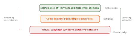
The hierarchy of verifiability in generative AI is:
Natural language: evaluation is subjective and expensive (human judgement required).
Code: evaluation is objective but incomplete (tests cover only finitely many inputs).
Mathematics: evaluation is objective and complete (formal proof checking is sound and decidable).
This hierarchy explains why mathematics is the ideal domain for training generative models with reinforcement learning: the reward signal is perfect.
This observation has profound implications for training. In reinforcement learning from human feedback (RLHF) [56], the reward model is a proxy for human preferences, and misalignment between the proxy and the true objective is a constant worry. In mathematical reasoning, the reward is the proof checker itself: a binary signal (valid or invalid) that is never wrong and never needs calibration. This makes mathematics a uniquely clean training ground for developing general reasoning capabilities.
Remark 1.
The availability of a perfect verifier does not make the generation problem easy. It merely makes the evaluation problem trivial. The search space of proofs is vast, the branching factor at each step is enormous, and most paths lead nowhere. Mathematics thus combines the best of both worlds for research: generating correct proofs is extremely hard, but verifying proposed proofs is extremely easy. This is the definition of an NP-like problem, and it is what makes mathematics such a fertile testbed for AI.
Mathematics is Harder Than Code
One might expect that the availability of perfect verification would make mathematical reasoning easier than code generation for AI systems. In practice, the opposite is true. As of 2025, the best language models solve approximately 70% of competition-level programming problems but fewer than 30% of competition-level mathematics problems at comparable difficulty levels [47]. Several factors explain this gap.
Flexibility of expression.
A correct Python function looks more or less the same regardless of who writes it. There are minor stylistic variations (variable names, choice of library functions), but the overall structure is largely determined by the specification. Mathematical proofs, by contrast, can look radically different while establishing the same result. Consider one of the oldest and most famous results in mathematics: the irrationality of .
Theorem 1 (Irrationality of ).
is irrational.
We now present two entirely different proofs of Theorem 1, illustrating how the same mathematical truth can be established through fundamentally different lines of reasoning.
Proof 1: By contradiction.
Suppose, for the sake of contradiction, that is rational. Then there exist integers and , with , such that , where is in lowest terms (i.e., ). Squaring both sides, we obtain , hence . This means is even, and since the square of an odd number is odd, itself must be even. Write . Then , so , which means is also even. But then both and are even, contradicting the assumption that is in lowest terms. Therefore is irrational.
Proof 2: By unique factorisation.
Suppose for positive integers . Then . By the fundamental theorem of arithmetic, the prime factorisation of has an even number of factors of 2 (since each factor of is doubled), while has an odd number of factors of 2 (one from the explicit factor of 2, plus an even number from ). Since a positive integer has a unique prime factorisation, and cannot be equal. Contradiction.
Both proofs are correct. Both establish the same result. But they employ different strategies, different intermediate lemmas, and different logical structures. The first proof is algorithmic: it follows a step-by-step descent argument. The second proof is structural: it leverages a deep property of the integers (unique factorisation) to derive a contradiction in a single stroke. A human mathematician recognises both as valid because they understand the meaning behind each step. A machine that processes proofs as token sequences must learn to recognise validity across these wildly different surface forms.
Exercise 1.
Give a third proof that is irrational, using the fact that if with positive integers, then with smaller numerator and denominator. (This is the “infinite descent” argument.) Explain how this proof differs structurally from the two given above.
Natural language ambiguity.
Mathematical proofs, as they appear in textbooks and journals, are written in natural language interspersed with formal notation. This creates a profound difficulty for AI systems. Consider the phrase “it is obvious that.” To a human mathematician, this is a signal that the omitted steps are routine and can be filled in by the reader. To a machine, it is a gap in the logical chain that could hide anything from a trivial calculation to a subtle error.
Professional mathematics is full of such shortcuts. Authors write “by a standard compactness argument” without spelling out the argument. They write “WLOG” (without loss of generality) and expect the reader to verify that the claimed reduction is valid. They write “the proof is similar to Theorem 3.2” without specifying which parts carry over and which require modification. Each of these conventions makes proofs shorter and more readable for human experts, but creates obstacles for AI systems that must fill in every detail.
Caution.
The gap between informal and formal mathematics is not merely a matter of verbosity. It is a semantic gap. An informal proof sketch might say “by continuity, the function attains its maximum on ,” invoking the extreme value theorem. Formalising this single sentence in a proof assistant might require 50 lines of code, including: showing that the function is continuous on the relevant domain, that the domain is compact, invoking the theorem from the library, and unpacking the resulting existential statement. The informal proof is not “wrong” but it elides enormous amounts of detail.
The verification gap.
The difficulty of natural language proofs creates what we call the verification gap: the distance between what a proof says and what a proof checker can verify. In code generation, this gap is small. A function written in Python can be executed directly; the language is its own verifier (via the interpreter and test suite). In mathematics, the gap is enormous. A proof written in English cannot be checked by any existing software without first being translated into a formal language, and this translation itself is a formidable AI challenge.
This gap has a direct consequence for training generative models. If we want to use proof correctness as a reward signal for reinforcement learning, we need proofs in a format that can be checked. This means either (a) training models to produce formal proofs directly, or (b) training models to translate informal proofs into formal ones. Both approaches have been pursued, and we will examine both in detail in subsequent sections.
Exercise 2.
Consider the following informal proof: “Since is continuous on and , by the intermediate value theorem there exists with .” List all the implicit assumptions and proof obligations that would need to be made explicit in a formal proof. How many separate lemmas or library theorems would be required?
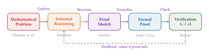
Historical Context: The Dream of Mechanical Reasoning
The aspiration to mechanise mathematical reasoning is as old as mathematics itself. We survey the key milestones, not merely for historical interest, but because each milestone shaped the conceptual toolkit that modern AI for mathematics inherits.
Historical Note.
Leibniz and the calculus ratiocinator (1684). Gottfried Wilhelm Leibniz dreamed of a “calculus of reasoning” that would reduce all intellectual disputes to computation. “When controversies arise,” he wrote, “there would be no more need for disputation between two philosophers than between two accountants. It would suffice for them to take their pencils in their hands, sit down to their slates, and say to each other: let us calculate.” This dream, though unrealised in Leibniz's lifetime, anticipates the core idea of formal verification: that correctness can be reduced to mechanical checking.
Hilbert's programme.
In 1900, David Hilbert presented 23 unsolved problems that would shape the course of twentieth-century mathematics. His second problem asked whether the axioms of arithmetic are consistent, a question that reveals a deeper ambition: to place all of mathematics on a secure, mechanically verifiable foundation. Hilbert's programme aimed to (1) formalise all of mathematics in a complete axiomatic system, (2) prove that the system is consistent (free from contradictions), and (3) develop a decision procedure that could determine the truth or falsity of any statement within the system.
Had Hilbert's programme succeeded, the story of AI for mathematics would be very different. Mathematics would be decidable: every question would have a mechanical answer. The role of creativity and intuition would be, in principle, eliminable. There would be no need for generative models that “discover” proofs, because a brute-force search would suffice.
Gödel's incompleteness.
In 1931, Kurt Gödel shattered this dream with his two incompleteness theorems [41]. The first theorem states that any consistent formal system capable of expressing basic arithmetic contains statements that are true but unprovable within the system. The second theorem states that such a system cannot prove its own consistency. These results did not merely show that Hilbert's programme could not be completed in its original form; they established a fundamental limit on what formal systems can achieve.
Theorem 2 (Gödel's First Incompleteness Theorem, informal).
For any consistent formal system that is capable of expressing basic arithmetic, there exist statements in the language of that are true (in the standard model of arithmetic) but not provable in .
The implications for AI are subtle and often misunderstood. Gödel's theorem does not mean that mathematical AI is impossible. It means that no single formal system can capture all mathematical truth, and that there will always be problems that require stepping outside the current framework to resolve. For practical purposes, the vast majority of mathematics that humans actually care about (analysis, algebra, geometry, number theory, combinatorics) can be formalised in standard foundations such as Zermelo-Fraenkel set theory with the axiom of choice (ZFC) or the calculus of inductive constructions used by Lean and Coq. The Gödelian limitations are real but remote: they concern statements at the frontier of mathematical logic, not the bread-and-butter theorems of working mathematicians.
Exercise 3.
Explain why Gödel's incompleteness theorems do not prevent an AI system from proving the vast majority of theorems in a typical undergraduate mathematics textbook. Under what circumstances would the incompleteness theorems become a practical obstacle?
Early automated reasoning.
The first automated theorem prover, the Logic Theorist, was created by Allen Newell and Herbert Simon in 1956 [57]. It proved 38 of the 52 theorems in Chapter 2 of Whitehead and Russell's Principia Mathematica, and for one theorem (2.85), it found a proof more elegant than the original. This early success fuelled enormous optimism. Simon famously predicted in 1958 that within ten years, a computer would prove a significant new mathematical theorem.
The prediction proved wildly optimistic. The combinatorial explosion of proof search, the difficulty of representing mathematical knowledge, and the brittleness of heuristic search strategies combined to ensure that automated theorem proving remained a niche endeavour for decades. Progress was steady but slow: resolution-based provers [22], tableaux methods, the development of SAT solvers, and eventually satisfiability modulo theories (SMT) solvers [26] expanded the class of problems that could be solved automatically, but always within narrow, well-defined logical fragments.
The four eras of mathematical AI.
We can roughly divide the history of AI for mathematics into four eras:
Symbolic era (1956–1990s): Hand-crafted heuristics, resolution provers, computer algebra systems. Success limited to narrow domains.
Statistical era (2000s–2010s): Machine learning applied to premise selection and proof guidance. Notable success with Vampire and E prover using learned heuristics [1].
Neural era (2017–2022): Deep learning for theorem proving. GPT-f [2], neural networks guiding Lean tactics. Proof of concept that language models can write proofs.
Generative era (2023–present): Large language models with reinforcement learning from proof verification feedback. AlphaProof [3], Lean Copilot, DeepSeek-Prover [4]. The era we are in now.
Each era built on the foundations laid by its predecessors, and the current generative era synthesises ideas from all three previous eras.
Exercise 4.
For each of the following systems, determine which era it belongs to and justify your classification: (a) the Boyer-Moore theorem prover, (b) HOL Light, (c) GPT-f, (d) AlphaProof, (e) Mathematica.
The key insight.
We arrive at the central observation that animates this entire chapter: formalization makes verification mechanical, and mechanical verification creates a perfect training signal for reinforcement learning. This insight connects the oldest dream in mathematical AI (Leibniz's calculus ratiocinator) to the newest techniques (RL with proof verification feedback). The dream of reducing reasoning to calculation has not been fully realised, but it has been partially realised in a form that Leibniz could not have anticipated: not as a universal decision procedure, but as a reward signal for training neural networks.
Key Idea.
The connection between formalization and machine learning can be stated as a simple equation: This equation is the foundation of the modern approach to AI for mathematics. It explains why formal proof assistants, originally developed for pure mathematical purposes, have become essential infrastructure for training generative models.
The social dimension.
There is another reason why mathematics matters for AI that is less often discussed: mathematics is fundamentally a social activity. Mathematicians do not work in isolation. They read each other's papers, attend each other's talks, build on each other's results, and occasionally disagree about whether a proof is correct. The history of mathematics is punctuated by famous errors: proofs that were accepted for years or decades before a flaw was found.
Example 1.
Famous mathematical errors.
In 1879, Alfred Kempe published a proof of the four-colour theorem. The proof was accepted for eleven years before Percy Heawood found a fatal error in 1890 [5]. The theorem was not correctly proved until 1976 (by Appel and Haken, using a computer).
In 1993, Andrew Wiles announced a proof of Fermat's Last Theorem. During peer review, a serious gap was found by Nick Katz. Wiles, with the help of Richard Taylor, spent another year repairing the proof before it was accepted in 1995 [6].
In 2012, Shinichi Mochizuki posted a 500-page proof of the abc conjecture using “inter-universal Teichmüller theory.” As of 2025, the mathematical community remains divided on whether the proof is correct, with prominent mathematicians on both sides of the debate.
These examples illustrate that even for human mathematicians, verification is not trivial. Formal verification eliminates this class of errors entirely.
Exercise 5.
Research one historical case where a mathematical proof was published and later found to contain an error. Describe: (a) the claimed result, (b) the nature of the error, (c) how the error was discovered, and (d) whether formal verification could have prevented the error. What does this tell us about the potential value of AI systems that produce formally verified proofs?
The Formalization of Mathematics
The idea of writing mathematics in a language so precise that a machine can check every step is both very old and very new. It is old because the dream of a universal formal language dates back to Leibniz and Frege. It is new because only in the last decade has formalization become practical enough to attract a critical mass of mathematicians, and only in the last few years has it become relevant to machine learning researchers.
In this section, we introduce the foundations of formal mathematics with an emphasis on the aspects that matter most for generative models: how mathematical statements are represented, how proofs are constructed and checked, and what kinds of mathematics have been formalised to date. The goal is not to turn the reader into a proof assistant expert, but to provide enough conceptual vocabulary to understand the AI systems that build on these foundations.
What Is Formalization?
Formalization is the process of translating mathematical statements and proofs from their natural, informal presentation (as found in textbooks, papers, and blackboard lectures) into a formal language that can be processed and checked by a computer. This process involves three key transformations:
Disambiguation. Every term must have a precise meaning. When a textbook says “let be a function,” the formalisation must specify: a function from what to what? Is it total or partial? Measurable? Continuous? The informal convention of leaving such details implicit must give way to explicit specification.
Completion. Every logical step must be justified. The phrase “it is easy to see that” must be replaced by an explicit chain of deductions. Every invocation of a theorem must be accompanied by a verification that its hypotheses are satisfied.
Encoding. The disambiguated, completed proof must be expressed in the syntax of a specific formal system. This involves choosing data structures for mathematical objects (natural numbers, real numbers, topological spaces), representing logical connectives and quantifiers, and organising the proof into a form that the proof checker can process.
Definition 1 (Formal proof).
A formal proof of a statement in a formal system is a finite sequence of statements such that each is either an axiom of or follows from earlier statements in the sequence by an inference rule of .
Remark 2.
This definition is intentionally austere. Real proof assistants use far richer notions of proof (proof terms, tactics, proof scripts), but the essential idea is the same: a proof is a chain of justified steps, and each step can be checked mechanically.
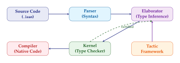
The critical property of formal proofs is that checking is mechanical. Given a formal proof, a computer program (the proof checker or “kernel”) can verify its correctness by inspecting each step. This program is typically small (a few thousand lines of code), well-understood, and trusted. The entire edifice of formalised mathematics rests on the correctness of this kernel, and significant effort is devoted to keeping it simple and auditable.
Example 2.
Consider the statement in the natural numbers. In informal mathematics, this is so obvious that it needs no proof. In a formal system based on the Peano axioms, the proof proceeds as follows: Even this trivial statement requires seven steps. The “obvious” fact is only obvious because humans have internalised the axioms and definitions so thoroughly that they are invisible.
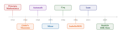
A Brief History of Formal Verification Systems
The development of formal verification systems spans more than a century. We highlight the milestones most relevant to the story of AI for mathematics.
Principia Mathematica (1910–1913).
Alfred North Whitehead and Bertrand Russell's monumental Principia Mathematica [58] was the first serious attempt to derive all of mathematics from a small set of logical axioms. The work is heroic in scope and notoriously difficult to read. Its notation is impenetrable by modern standards. The proof that does not appear until page 379 of Volume I. Yet Principia established the principle that mathematics can be formalised, and that principle has never been overturned.
Automath (1968).
Nicolaas de Bruijn's Automath was the first computer language designed specifically for expressing mathematical proofs in a form that a computer could check [59]. Automath introduced several ideas that remain central to modern proof assistants: the use of type theory as a logical foundation, the representation of proofs as terms in a typed lambda calculus, and the principle that proof checking reduces to type checking.
Mizar (1973).
The Mizar system, created by Andrzej Trybulec, took a different approach: it aimed to make formalised mathematics as close as possible to the way mathematicians actually write [60]. Mizar proofs read almost like (very precise) English. The Mizar Mathematical Library, built over decades by the Mizar community, contains over 60,000 formalised theorems and represents one of the largest bodies of formalised mathematics in existence.
Coq (1984).
The Coq proof assistant, developed by Thierry Coquand and Gérard Huet at INRIA, is based on the Calculus of Inductive Constructions (CIC), a powerful type theory that can express virtually all of standard mathematics [61]. Coq introduced tactics: high-level proof commands that automate routine steps and allow the user to guide the proof at a strategic level. Notable achievements formalised in Coq include the four-colour theorem [62] and the Feit-Thompson odd-order theorem [63].
Isabelle/HOL (1986).
Lawrence Paulson's Isabelle is a generic proof assistant that supports multiple logical foundations, with Higher-Order Logic (HOL) being the most widely used [64]. Isabelle's “Sledgehammer” tool automatically calls external automated theorem provers (ATP) to discharge proof obligations, bridging the gap between interactive and automated theorem proving [65].
Lean (2013–present).
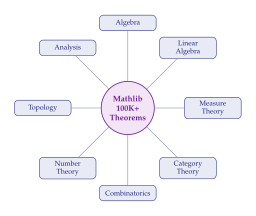
The Lean proof assistant, created by Leonardo de Moura at Microsoft Research and now developed as an open-source project, has become the most active venue for both mathematical formalisation and AI for mathematics [66]. Lean 4, the current version, is both a proof assistant and a general-purpose programming language, making it particularly well-suited for integration with machine learning systems. Its mathematical library, Mathlib [67], is the largest unified collection of formalised mathematics, containing over 100,000 theorems as of 2025.
A note on foundations.
The choice of logical foundation matters more than it might seem. Lean and Coq use type theory (specifically, variants of the Calculus of Inductive Constructions). Isabelle/HOL uses higher-order logic. Mizar uses set theory. These foundations are not identical in expressive power, though for practical purposes they can all express the same mathematics. The choice of foundation affects:
Syntax: how theorems and proofs look on the screen.
Automation: what the proof assistant can fill in automatically.
Libraries: what has already been formalised and is available for reuse.
Community: who is developing the system and what kinds of mathematics they prioritise.
For AI purposes, the choice of foundation translates directly into a choice of programming language for the generated proofs. A model trained to generate Lean proofs cannot generate Coq proofs without retraining, just as a model trained to generate Python code cannot generate Rust code. This fragmentation of the formal mathematics ecosystem is a significant practical challenge.
Exercise 6.
Look up the formalised statement of the fundamental theorem of algebra in both Lean (Mathlib) and Coq (the math-comp library). Compare the two formalisations. How do they differ in notation, structure, and the mathematical prerequisites they depend on? What challenges would this pose for a model attempting to translate between the two?
Type Theory and the Curry-Howard Correspondence
Most modern proof assistants (Lean, Coq, Agda) are based on type theory rather than set theory as their logical foundation. This choice, which may seem like a minor technical detail, has profound consequences for how proofs are represented and, consequently, for how generative models interact with formal mathematics.
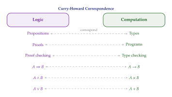
The central idea is beautifully simple, and it is known as the Curry-Howard correspondence (or the “proofs-as-programs” interpretation). The correspondence establishes a deep analogy between two seemingly unrelated domains: logic and computation.
Definition 2 (Curry-Howard correspondence, informal).
The Curry-Howard correspondence is the observation that:
Propositions correspond to types.
Proofs correspond to programs (terms).
Proof checking corresponds to type checking.
Under this correspondence, proving a theorem amounts to constructing a program of a given type, and checking the proof amounts to checking that the program is well-typed.
Let us unpack this with concrete examples.
Propositions as types.
Consider the logical proposition (“if , then ”). Under the Curry-Howard correspondence, this proposition corresponds to the function type . A proof of is a function that takes a proof of as input and produces a proof of as output. This makes intuitive sense: if you can show me how to transform any evidence for into evidence for , then you have shown that implies .
Example 3.
The proposition “if is even, then is even” corresponds to a function of type . A proof of this proposition is a program that takes a witness that is even (say, a number such that ) and produces a witness that is even (namely, , so is the witness).
Logical connectives as type constructors.
The correspondence extends to all logical connectives:
| Logic | Type Theory | Proof/Program |
| (and) | (product) | A pair with and |
| (or) | (sum) | Either a proof of or a proof of |
| (implies) | (function) | A function from proofs of to proofs of |
| (dep. function) | A function assigning a proof of to each | |
| (dep. pair) | A witness together with a proof of | |
| (false) | (empty type) | No program of this type exists |
The last row is particularly elegant: the proposition “False” (a contradiction) corresponds to the empty type, which has no inhabitants. This means that a consistent logical system cannot prove “False,” just as a well-typed programming language cannot produce a term of the empty type.
Insight.
The Curry-Howard correspondence transforms theorem proving into programming. This is not merely a conceptual analogy; it is an operational equivalence. When a generative model produces a proof in Lean or Coq, it is literally writing a program that will be type-checked by the proof assistant's kernel. This means that techniques from program synthesis, including neural code generation, can be directly applied to theorem proving.
Exercise 7.
Under the Curry-Howard correspondence, a proof of is a pair where and .
What is the proof of as a program? (Hint: it is a function that takes a pair and swaps its components.)
What is the proof of as a program?
Why does the empty type (corresponding to , falsehood) have no constructors? What would it mean if it did?
The Calculus of Inductive Constructions
The logical foundation used by both Lean and Coq is the Calculus of Inductive Constructions (CIC), a dependent type theory that extends the Curry-Howard correspondence to handle the full richness of mathematical reasoning. We provide a high-level overview; the reader interested in formal details should consult Bertot and Castéran [61] or the Lean documentation [66].
Universes.
CIC organises types into a hierarchy of universes: , , , and so on. The universe contains propositions (statements that are either true or false). The universe contains ordinary types (natural numbers, lists, functions). Higher universes contain types of types, enabling the construction of mathematical structures at arbitrary levels of abstraction.
Inductive types.
The “Inductive” in CIC refers to the ability to define new types by specifying their constructors: the ways in which elements of the type can be built. The natural numbers, for example, are defined by two constructors:
(zero is a natural number), and
(the successor of a natural number is a natural number).
Every natural number is either or for some , and this exhaustive case analysis is the foundation of proof by induction. More complex mathematical objects (lists, trees, groups, topological spaces) are defined as more elaborate inductive types.
Dependent types.
The key feature that makes CIC powerful enough for mathematics is dependent types: types that can depend on values. For example, the type of lists of length exactly depends on the natural number . In a mathematical context, the type of proofs that is prime depends on the value of . Dependent types allow the type system to express arbitrarily complex mathematical properties, and type checking enforces these properties automatically.
Example 4.
Consider the function that concatenates two vectors: The type of this function guarantees that the output vector has length . This is not a runtime check or a test; it is a compile-time guarantee enforced by the type checker. If the implementation does not produce a vector of exactly the right length, the code will not type-check. This is the power of dependent types: the types are the specification.
Exercise 8.
In a dependently typed language, define the type of a function that takes a natural number and returns a proof that . What would the Curry-Howard interpretation of this type be as a logical proposition? Why is this seemingly trivial statement non-trivial to prove in a formal system based on the Peano axioms? (Hint: addition is defined by recursion on its first argument.)
What Can Be Formalised?
A natural question is: how much of mathematics can actually be formalised? The answer is both encouraging and humbling.
In principle: virtually everything.
The standard foundations of mathematics (ZFC set theory, or equivalently the Calculus of Inductive Constructions) are powerful enough to express virtually all of the mathematics that humans have ever developed. Analysis, algebra, topology, number theory, combinatorics, probability theory, differential geometry: all can be (and to varying degrees have been) formalised in systems like Lean, Coq, and Isabelle.
In practice: a growing fraction.
As of 2025, the largest formalised library is Lean's Mathlib [67], which contains:
Over 100,000 theorems and lemmas.
Formalised coverage of undergraduate mathematics: linear algebra, group theory, ring theory, real and complex analysis, measure theory, topology.
Significant graduate-level material: commutative algebra, algebraic geometry (schemes), category theory, representation theory.
Notable individual achievements: the formalisation of Fermat's Last Theorem is underway (as a community project led by Kevin Buzzard at Imperial College London).
Yet Mathlib covers only a small fraction of the total body of known mathematics. The Mathematical Reviews database (MathSciNet) contains over 4 million reviews of mathematical papers. Even if each Mathlib theorem corresponds to several journal theorems, the gap is enormous. This gap is both a challenge and an opportunity for generative models: if AI can accelerate formalisation, the resulting formal libraries would be vastly more valuable as training data than the current collections.
Historical Note.
The Flyspeck project. In 1998, Thomas Hales announced a proof of the Kepler conjecture (that the densest packing of spheres in three dimensions is the face-centred cubic packing). The proof was 300 pages long and relied on extensive computer calculations. The referees spent four years reviewing it and concluded that they were “99% certain” it was correct, but could not fully verify the computational parts. Frustrated by this uncertainty, Hales launched the Flyspeck project to produce a complete formal verification. The project, which used Isabelle and HOL Light, was completed in 2014 [7]. Flyspeck demonstrated both the power of formal verification (the proof is now beyond doubt) and its cost (the formalisation took a team of researchers 16 years).
What Cannot Be Formalised: Gödel's Shadow
We have established that virtually all of known mathematics can be formalised. But Gödel's incompleteness theorems (Theorem 4) tell us that no formal system can capture all mathematical truth. What are the implications for AI?
Proposition 1 (Limits of formal verification).
For any consistent formal system capable of expressing arithmetic:
There exist true arithmetic statements that cannot prove.
cannot prove its own consistency.
Any AI system that generates proofs within inherits these limitations: there are true statements it cannot prove, no matter how intelligent it is.
Remark 3.
The practical impact of Gödel's theorems on AI for mathematics is often overstated. The unprovable statements constructed in Gödel's proof are highly artificial (self-referential sentences of the form “this statement is not provable in ”). The vast majority of mathematics that humans find interesting and useful is provable in standard foundations. The Riemann Hypothesis, the P versus NP problem, and the Navier-Stokes existence and smoothness problem are not known to be independent of ZFC; they are simply hard. For an AI system working within Lean or Coq, Gödel's theorem is a theoretical boundary, not a practical obstacle.
That said, the incompleteness theorems do have two important consequences for the design of AI systems:
No universal prover. There can be no AI system that proves all true mathematical statements, even in principle. Any prover must eventually encounter statements that are true but beyond its reach. This means that the “solve all of mathematics” goal is not merely practically difficult but logically impossible.
Foundation choice matters. Different formal systems can prove different sets of theorems. An AI system trained on proofs in one foundation might not transfer to another. The choice of formal system is a design decision with real consequences.
Exercise 9.
Consider an AI system that generates proofs in Lean (which is based on CIC, roughly equivalent in strength to ZFC). Can this system prove the consistency of Lean's own type theory? Why or why not? What would happen if we added the consistency of CIC as an extra axiom? Would this resolve the problem or merely shift it?
Mathlib: A Case Study in Large-Scale Formalisation
No discussion of formalization in the context of AI would be complete without a detailed look at Mathlib, the mathematical library for Lean. Mathlib is not merely a collection of theorems; it is a dataset, and understanding its structure is essential for understanding how generative models are trained on formal mathematics.
Scale and scope.
As of early 2025, Mathlib contains approximately:
100,000+ formalised definitions and theorems.
1.5 million lines of Lean code.
Coverage of 30+ branches of mathematics.
Contributions from 400+ mathematicians and computer scientists worldwide.
The library is organised hierarchically. At the foundation lie basic type theory, logic, and natural number arithmetic. Above this sit the algebraic hierarchy (monoids, groups, rings, fields, modules, algebras), the topological hierarchy (topological spaces, metric spaces, uniform spaces, compact spaces), and the analytical hierarchy (limits, continuity, differentiation, integration, measure theory). Each layer builds on those below, and the dependency graph is both deep and wide.
As a training dataset.
From the perspective of generative AI, Mathlib offers several advantages as a training dataset:
Ground truth. Every theorem in Mathlib has been verified by Lean's kernel. There are no errors, no gaps, no hand-waving. This makes it a uniquely clean dataset compared to, say, mathematics scraped from the internet.
Structured metadata. Each theorem has a name, a precise statement, a proof, a list of dependencies, and a position in the import hierarchy. This metadata supports a variety of learning tasks: next-theorem prediction, proof synthesis, premise selection, and more.
Diverse proof strategies. Mathlib proofs range from one-line tactic invocations (“
simp”) to multi-hundred-line constructions involving dozens of intermediate lemmas. This diversity provides training signal at multiple scales.Living codebase. Mathlib is actively developed, with new theorems added daily. This creates a natural evaluation methodology: can a model prove theorems that were added after its training data was collected?
Key Idea.
Mathlib occupies a unique position in the AI for mathematics ecosystem: it is simultaneously a mathematical achievement (the largest unified formalisation of mathematics), a training dataset (ground-truth proof data with rich metadata), and an evaluation benchmark (new theorems provide fresh test cases). This triple role makes it indispensable for research on generative models for mathematics.
Exercise 10.
Visit the Mathlib documentation (available online at
leanprover-community.github.io/mathlib4_docs/) and find
the formalised statement of the following theorems:
The Bolzano-Weierstrass theorem (every bounded sequence in has a convergent subsequence).
Lagrange's theorem (the order of a subgroup divides the order of the group).
The fundamental theorem of calculus.
For each, note how the formal statement differs from the informal version you learned in a textbook. What additional hypotheses or type annotations are required?
The Landscape of AI for Mathematics
Having established the foundations of mathematical formalization, we now survey the landscape of AI approaches to mathematical reasoning. This landscape is rich and rapidly evolving, with roots in classical automated theorem proving, branches extending through modern deep learning, and new shoots emerging from the intersection of large language models and formal verification.
Understanding this landscape is essential for appreciating the generative models that are the focus of the remainder of this chapter. Each approach brings distinct strengths, and the most powerful modern systems combine ideas from multiple traditions.
A Taxonomy of Approaches
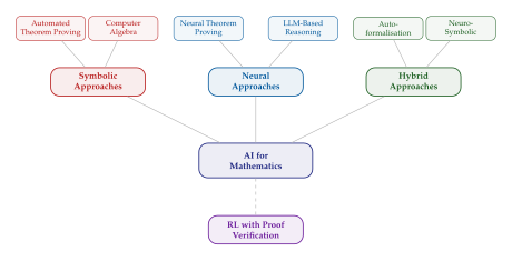
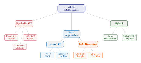
We organise the space of AI for mathematics into four broad categories, each defined by its relationship to formal and informal mathematical language:
Symbolic Automated Theorem Proving (ATP). Systems that operate entirely within formal logic, using search and inference rules to derive proofs. Examples include resolution provers (Vampire, E), tableaux provers, and SAT/SMT solvers (Z3, CVC5).
Neural Theorem Proving (NTP). Systems that use neural networks to guide proof search within a formal proof assistant. The neural network suggests tactics or proof steps, and the proof assistant verifies each step. Examples include GPT-f [2], PACT [8], and ReProver [9].
LLM-Based Mathematical Reasoning. Systems that use large language models to reason about mathematics in natural language, without necessarily producing formal proofs. Examples include Minerva [10], chain-of-thought reasoning [11], and tool-augmented approaches.
Hybrid Neuro-Symbolic Approaches. Systems that combine neural language models with formal verification, typically through autoformalization (translating informal mathematics to formal proofs). Examples include AlphaProof [3], DeepSeek-Prover [4], and Lean Copilot.
The Pre-Generative Era: Symbolic Methods
Before neural networks entered the picture, automated theorem proving was a purely symbolic enterprise. The fundamental idea is simple in principle: given a set of axioms and a goal, systematically search the space of possible derivations until a proof is found. In practice, the search space is astronomically large, and the art of ATP lies in finding good strategies to prune it.
Resolution.
The most influential technique in classical ATP is resolution, introduced by Alan Robinson in 1965 [22]. Resolution works in first-order logic with clausal form. Every formula is converted to a set of clauses (disjunctions of literals), and the resolution rule derives new clauses from existing ones by identifying complementary literals. If the empty clause is derived, the original formula set is unsatisfiable, which (by refutation) proves the desired theorem.
Resolution is complete for first-order logic: if a theorem is true, resolution will eventually find a proof. But “eventually” can mean “after the heat death of the universe.” The practical success of resolution provers like Vampire [68] and E [69] depends on sophisticated heuristics for selecting which clauses to resolve, which substitutions to try, and which derived clauses to retain.
SAT and SMT solvers.
The Boolean satisfiability problem (SAT) asks whether there exists an assignment of truth values that satisfies a given propositional formula. Despite being NP-complete, modern SAT solvers can handle instances with millions of variables, thanks to techniques like conflict-driven clause learning (CDCL). Satisfiability Modulo Theories (SMT) extends SAT with background theories (arithmetic, arrays, bit vectors), enabling reasoning about richer domains [26].
SAT/SMT solvers have proven remarkably effective for certain mathematical problems, particularly in combinatorics. Notable examples include the resolution of the Boolean Pythagorean triples problem by Heule, Kullmann, and Marek [70], which produced a proof of 200 terabytes, the largest proof ever generated at the time.
Strengths and limitations.
Symbolic ATP methods have two great strengths: they produce verified proofs (every step is logically justified), and they can handle problems with deep combinatorial structure. Their main weakness is that they lack mathematical intuition: they cannot read a theorem statement and “see” the right proof strategy. They explore the search space blindly, guided only by syntactic heuristics. This makes them excellent at proving lemmas that require mechanical bookkeeping but poor at proving theorems that require creative insight.
Exercise 11.
Consider the following set of clauses in propositional logic:
Apply the resolution method to derive the empty clause, thereby showing that this set of clauses is unsatisfiable. Draw the resolution tree. How many resolution steps are required?
The Neural Revolution: Learning to Prove
The entry of neural networks into theorem proving marked a qualitative shift. Instead of relying on hand-crafted heuristics, neural systems learn proof strategies from data. The key insight is that a neural network can be trained to predict which proof step (tactic, lemma, or transformation) is most likely to make progress, given the current proof state.
Premise selection.
The earliest applications of machine learning to theorem proving focused on premise selection: given a conjecture to prove, which lemmas and definitions from the library are most likely to be useful? This is a classification problem: for each potential premise, predict whether it will appear in the proof. Early work by Urban [1] and Kaliszyk [71] showed that even simple machine learning models (k-nearest neighbours, naive Bayes) could significantly outperform hand-crafted heuristics at this task.
GPT-f and the language model approach.
The paper that launched the neural theorem proving era was GPT-f by Polu and Sutskever [2], which demonstrated that a GPT-style language model, fine-tuned on Lean proofs, could generate valid proof steps. The approach is conceptually simple: the model takes the current proof state (the goals and hypotheses) as input and generates the next tactic as output. If the generated tactic is accepted by the proof assistant, the proof state advances; otherwise, the model tries again.
GPT-f proved 56.5% of test theorems from a Lean benchmark, outperforming the previous state of the art. More importantly, it found 23 new proofs of theorems in Mathlib that had been manually proved by human mathematicians, several of which were shorter than the original proofs. This demonstrated that language models could not merely imitate human proofs but occasionally improve upon them.
PACT and expert iteration.
Han et al. introduced PACT (Proof Artifact Co-Training), which interleaves proof search with model training [8]. The model generates proofs, the successful proofs are added to the training set, and the model is retrained on the expanded dataset. This expert iteration loop (also known as “self-play for theorem proving”) allows the model to bootstrap from a small initial dataset of human proofs to a much larger dataset of machine-generated proofs.
ReProver and LeanDojo.
Yang et al. developed LeanDojo, a framework for extracting training data from Lean and interacting with the proof assistant programmatically, along with ReProver, a retrieval-augmented neural theorem prover [9]. ReProver uses a retrieval module to select relevant premises from Mathlib before generating tactics, addressing a key bottleneck: the vast size of the library makes it impossible for the model to “memorize” all relevant lemmas.
Remark 4.
A recurring theme in neural theorem proving is the interplay between generation (suggesting proof steps) and verification (checking that the steps are valid). The proof assistant serves as an oracle that provides immediate, deterministic feedback on every generated step. This tight feedback loop is what makes theorem proving a more tractable RL environment than, say, open-ended text generation, where the quality of a response cannot be determined until a human reads it.
LLMs Enter the Arena
The release of GPT-4 [72] and subsequent large language models marked a new era for mathematical AI. These models, trained on vast corpora of internet text (including mathematical textbooks, papers, and forum discussions), demonstrated an unexpected capacity for mathematical reasoning without any specialized training on formal mathematics.
Chain-of-thought reasoning.
Wei et al. [11] showed that prompting a language model to “think step by step” dramatically improves its performance on mathematical word problems. Instead of jumping directly from problem to answer, the model generates a sequence of intermediate reasoning steps, each building on the last. This chain-of-thought approach does not guarantee correctness (the reasoning can still be flawed), but it provides a scaffold that makes errors easier to detect and correct.
Minerva and mathematical specialisation.
Google's Minerva [10] fine-tuned a large language model on a curated dataset of mathematical text, including textbooks, papers, and web content with mathematical notation. Minerva achieved state-of-the-art performance on several mathematical benchmarks, including MATH (a dataset of competition-level problems) and GSM8K (a dataset of grade-school math problems), without using any formal proof assistant.
The gap between informal and formal.
The remarkable success of LLMs on informal mathematical reasoning comes with an important caveat: the outputs are not verified. An LLM can produce a fluent, plausible-looking proof that contains subtle logical errors. It can invoke theorems that do not exist (“hallucinated” lemmas). It can skip steps that seem obvious but are actually wrong. Without formal verification, there is no reliable way to distinguish a correct proof from a convincing fake.
This limitation is not merely theoretical. Studies have shown that LLMs produce mathematical errors at significant rates [73], including errors that are difficult for human reviewers to detect. The errors tend to cluster at “hard” steps where genuine mathematical insight is required, precisely the steps where AI assistance would be most valuable.
Caution.
The fluency of LLM-generated mathematics is both its greatest strength and its greatest danger. A proof that “reads well” is not necessarily correct, and the very fluency of the output can lull the reader into accepting errors that would be caught in a formal proof. This is why the integration of LLMs with formal verification is so important: the LLM provides mathematical intuition and natural language fluency, while the proof assistant provides the rigorous checking that intuition alone cannot supply.
Exercise 12.
Ask a large language model to prove that every continuous function is uniformly continuous. (This is true, by the Heine-Cantor theorem.) Carefully check each step of the model's output. Does the model correctly invoke compactness? Does it handle the - argument correctly? Identify any errors or unjustified steps.
Mathematical olympiad performance.
The most dramatic demonstration of LLM mathematical capabilities has come from competition mathematics. The International Mathematical Olympiad (IMO) has served as a high-profile benchmark. While pure LLM-based approaches (without formal verification) have shown impressive results on simpler competition problems, they struggle with the multi-step reasoning required by IMO-level problems. This performance gap has driven the field toward hybrid approaches that combine the intuition of LLMs with the rigour of formal verification.
Example 5.
IMO 2024 Problem 1 (simplified). Consider a function satisfying for all integers . Determine all such functions. This problem requires: (a) substituting specific values to derive constraints, (b) recognising a functional equation pattern, and (c) verifying the candidate solution. A pure LLM approach might correctly execute steps (a) and (c) but fail at the creative insight required for step (b). A hybrid approach can use the LLM for intuition and the proof assistant for verification.
The Key Insight: Autoformalization
The previous subsections revealed a tension. Symbolic ATP systems produce verified proofs but lack mathematical intuition. LLMs possess mathematical intuition but produce unverified output. Neural theorem provers bridge this gap by using neural networks to guide formal proof search, but they are limited by the availability of formal training data.
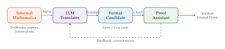
Autoformalization resolves this tension by using language models to translate informal mathematics (written in natural language with mathematical notation) into formal mathematics (written in Lean, Coq, or Isabelle). The idea is to leverage the vast quantities of informal mathematical text available on the internet and in textbooks, while using formal proof assistants to verify the results.
Definition 3 (Autoformalization).
Autoformalization is the task of automatically translating informal mathematical statements and proofs into formal representations that can be processed by a proof assistant. It encompasses:
Statement formalisation: translating a natural language theorem statement into a formal type.
Proof formalisation: translating a natural language proof into a sequence of formal tactics or a proof term.
Concept alignment: mapping informal mathematical concepts to their formal counterparts in a library like Mathlib.
The significance of autoformalization for generative models cannot be overstated. It creates a data flywheel: informal mathematics (abundant but unverified) is translated to formal mathematics (scarce but verified), which produces new training data for both the translation model and the proof generation model. Each turn of the wheel increases the pool of formal mathematics available for training, which in turn improves the models, which in turn enables more formalisation.
Early work.
The idea of autoformalization was articulated by Szegedy in 2020 [74], who argued that autoformalization could be the “Rosetta Stone” connecting the vast informal mathematical literature to formal proof assistants. Wu et al. [75] demonstrated that large language models could translate informal mathematical statements into formal Isabelle code with surprising accuracy, even without fine-tuning on paired informal-formal data.
The role of verification.
What makes autoformalization particularly powerful is that the translations can be verified. If the LLM translates an informal theorem into a formal statement and the formal statement type-checks in Lean, we know the translation is at least syntactically valid. If the LLM also provides a proof and the proof is accepted by the kernel, we know the formal statement is true (in the formal system). The remaining question is whether the formal statement faithfully captures the intent of the informal statement, and this is the primary source of error in autoformalization.
Exercise 13.
Consider the informal statement: “Every continuous function on a closed interval attains its maximum.” Write down two different formal statements in pseudo-Lean that could be considered valid formalizations of this statement. How do they differ? Which one more faithfully captures the informal intent? (Hint: consider whether the interval should be non-empty, whether “continuous” means continuous on the whole real line restricted to the interval or continuous with respect to the subspace topology, and whether “attains its maximum” means there exists a point where the maximum is achieved or that the supremum is a maximum.)
Reinforcement Learning with Proof Verification
The final piece of the modern mathematical AI puzzle is the use of reinforcement learning (RL) to train models that generate proofs, using the proof assistant as the reward signal. This approach combines the pattern recognition capabilities of neural networks with the rigorous checking capabilities of formal systems.
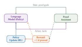
The setup is natural:
State: the current proof state (goals and hypotheses) in the proof assistant.
Action: a tactic or proof step generated by the model.
Reward: if the proof is completed (all goals discharged), otherwise (with optional intermediate rewards for making progress).
Environment: the proof assistant itself, which deterministically updates the proof state in response to each action.
This formulation has several attractive properties. The environment is deterministic: the same tactic always produces the same state transition. The reward is binary and reliable: either the proof compiles or it does not. The state is fully observable: the proof assistant displays all current goals and available hypotheses. These properties make theorem proving a “clean” RL environment, free from the noise and partial observability that complicate many other RL applications.
Key Idea.
Theorem proving in a formal proof assistant can be cast as a Markov Decision Process (MDP) with deterministic transitions and a binary reward signal. This makes it an ideal testbed for RL algorithms, as the only source of difficulty is the enormous branching factor of the action space (the number of possible tactics at each step), not the noise or ambiguity that afflict most RL environments.
AlphaProof.
In 2024, DeepMind's AlphaProof system [3] demonstrated the power of this approach by solving four of six problems from the International Mathematical Olympiad (IMO), achieving a score that would have earned a silver medal. AlphaProof combined a language model (for translating competition problems into formal statements) with a reinforcement learning system (for searching for formal proofs in Lean). The system was trained through millions of iterations of self-play, generating proof attempts, verifying them, and using the results to improve the model.
DeepSeek-Prover.
Xin et al. [4] developed DeepSeek-Prover, which uses a large language model fine-tuned on Lean proofs with RL from proof verification feedback. The key innovation is the use of whole-proof generation: instead of generating one tactic at a time (as in GPT-f), DeepSeek-Prover generates entire proofs in a single pass, relying on the Lean compiler to verify the result. This approach is simpler and more scalable than step-by-step search, at the cost of requiring the model to plan the entire proof structure in advance.
Exercise 14.
Design a reward function for training a language model to generate Lean proofs using RL. Consider the following questions:
Should the reward be purely binary ( for a complete proof, otherwise), or should there be intermediate rewards for partial progress (e.g., reducing the number of remaining goals)?
What are the advantages and disadvantages of whole-proof generation (generating the entire proof at once and checking it) versus step-by-step generation (generating one tactic at a time and checking after each step)?
How should the system handle proofs that are correct but unnecessarily long or inelegant? Should proof length be penalised?
Comparison with Code Generation
Throughout this section, we have drawn comparisons between mathematical reasoning and code generation. It is worth making these comparisons explicit, as the similarities and differences illuminate the unique challenges and opportunities of AI for mathematics.
| Property | Code Generation | Theorem Proving |
| Verification | Tests (incomplete) | Proof checker (complete) |
| Output format | Executable code | Proof term / tactic script |
| Correctness notion | Passes all tests | Type-checks |
| Search space | Function space | Proof space |
| Feedback granularity | Per test case | Per tactic |
| Training data | GitHub (billions of files) | Mathlib (100K theorems) |
| Natural language gap | Small (code is precise) | Large (proofs are informal) |
| Branching factor | Moderate | Very high |
The most striking difference is the data asymmetry. GitHub contains billions of source files in dozens of programming languages. Mathlib contains 100,000 theorems in a single proof assistant. This three-to-four order-of-magnitude gap in training data is the single biggest obstacle to applying the techniques that succeeded in code generation (large-scale pretraining on source code) to theorem proving.
Challenge 1.
The data scarcity problem in formal mathematics: there is not enough formal proof data to train large language models using the same recipes that work for code generation. This challenge motivates autoformalization (creating more formal data from informal sources), expert iteration (creating more formal data through self-play), and curriculum learning (training models on progressively harder problems).
The second major difference is the verification quality. Code generation uses tests, which are incomplete: a function can pass all tests and still be wrong. Theorem proving uses formal verification, which is complete: a proof that type-checks is guaranteed to be correct (modulo the consistency of the underlying foundations, which is universally assumed). This higher-quality verification signal is both a blessing (it enables cleaner RL training) and a curse (it sets a higher bar for the model to clear).
Preview: The Road Ahead
Having surveyed the landscape, we now have the conceptual vocabulary needed to understand the specific systems and techniques that will be explored in the remainder of this chapter. The road ahead covers the following territory:
Neural theorem proving in depth: how models represent proof states, generate tactics, and search the proof tree.
Autoformalization: translating between informal and formal mathematics using language models, with a focus on training data creation and evaluation.
RL for mathematics: the specific RL algorithms, reward structures, and training curricula used to develop mathematical reasoning capabilities.
Evaluation and benchmarks: how we measure progress in AI for mathematics, from simple competition problems to research-level conjectures.
Open problems: the frontier challenges that remain, including reasoning about novel mathematical structures, generating readable proofs, and approaching research-level mathematics.
Each of these topics builds on the foundations laid in this section: the formalization of mathematics provides the language, the taxonomy of approaches provides the conceptual framework, and the RL-with- verification paradigm provides the training methodology.
Conjecture 1.
Within the next decade, AI systems will be capable of routinely formalising the proofs in a typical graduate-level mathematics textbook, thereby creating a self-sustaining cycle in which formal verification data begets better models, which beget more formal verification data. The bottleneck will not be proof generation but problem generation: finding the right conjectures to prove.
Introduction to Lean 4
If mathematics is the language of certainty, then Lean 4 is its compiler. In this section we give a self-contained, tutorial-style introduction to Lean 4, the interactive theorem prover that has become the de facto standard platform for AI-assisted formal mathematics. We assume no prior experience with dependent type theory; every concept is built from the ground up with worked examples.
Historical Note.
Leonardo de Moura began the Lean project at Microsoft Research in 2013 [12]. Lean 1 and 2 were research prototypes; Lean 3, released in 2017, attracted a vibrant community through the mathlib library. Lean 4, a complete rewrite released in 2021, is both a general-purpose programming language and a theorem prover, with a self-hosted compiler, hygienic macro system, and first-class metaprogramming [13]. Since 2023 the project is maintained by the Lean Focused Research Organisation, independent of Microsoft.
Propositions as Types, Proofs as Programs
The philosophical foundation of Lean is the Curry–Howard correspondence: every mathematical proposition is a type, and every proof of that proposition is a term (program) inhabiting that type.
Definition 4 (Curry–Howard Correspondence).
Let denote the universe of propositions. For every proposition , a proof of is a term . Logical connectives correspond to type formers:
| Logic | Type Theory | Lean Syntax |
| (product) | P $$ Q | |
| (sum) | P $$ Q | |
| (function) | P -> Q | |
Not P | ||
| (dependent function) | forall x, P x | |
| (dependent pair) | exists x, P x |
Key Idea.
To prove a proposition in Lean, you construct a term of the corresponding type. To prove , you write a function that takes a proof of and returns a proof of . Logic becomes programming.
Let us see this in action with the simplest possible theorem:
Example 6 (Two Plus Two).
The following Lean 4 code proves that :
theorem two_plus_two : 2 + 2 = 4 := by
rfl
rfl (reflexivity) works because Lean's kernel reduces
2 + 2 to 4 by computation, recognising that the two sides
are definitionally equal.Example 7 (A Simple Implication).
To prove (every proposition implies itself):
theorem self_implication (P : Prop) : P -> P := by
intro h -- assume P holds; call the proof h
exact h -- provide h as the proof of the goal P
The Type Hierarchy
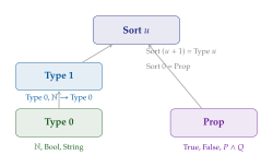
Lean organises types into a hierarchy of universes:
Definition 5 (Universe Hierarchy).
Lean 4 has three families of universes:
(alias ): the universe of propositions. All proofs of a proposition are considered equal (proof irrelevance).
(alias ): the universe of data types at level . contains ordinary types like , , .
: the general universe at level . It unifies and into a single hierarchy.
Remark 5.
Proof irrelevance in means that if then . This is essential for mathematical practice: we do not distinguish between two proofs of the same theorem. In contrast, distinguishes inhabitants: the natural numbers and are different terms of type .
Natural Numbers and Induction
The natural numbers are defined as an inductive type:
inductive Nat where
| zero : Nat
| succ (n : Nat) : Nat
Every natural number is either zero or the successor of
another natural number. This gives us the recursor (induction
principle) for free.
Theorem 3 (Principle of Mathematical Induction in Lean).
For any property , if
holds (base case), and
for all , (inductive step),
then holds for all . In Lean:
theorem Nat.rec_on {P : Nat -> Prop}
(n : Nat) (h0 : P 0) (hs : forall k, P k -> P (k + 1)) : P n
Example 8 (Commutativity of Addition).
We prove for all natural numbers. The proof proceeds by induction on :
theorem add_comm (n m : Nat) : n + m = m + n := by
induction n with
| zero => simp
| succ k ih =>
simp [Nat.succ_add, Nat.add_succ]
exact ih
induction tactic generates two goals: the base case
(, solved by simp) and the inductive step
(, solved using the induction hypothesis
ih and simplification lemmas).Example 9 (Associativity of Addition).
theorem add_assoc (a b c : Nat) : (a + b) + c = a + (b + c) := by
induction c with
| zero => simp
| succ k ih =>
simp [Nat.add_succ]
exact ih
Insight.
Notice that both proofs follow the same pattern: induction, then simplification using definitional equalities. This pattern recurs throughout formal mathematics and is precisely what neural theorem provers learn to recognise.
Logic in Lean
Lean defines logical connectives as inductive types:
-- Conjunction (And)
structure And (P Q : Prop) where
left : P
right : Q
-- Disjunction (Or)
inductive Or (P Q : Prop) where
| inl (h : P) : Or P Q
| inr (h : Q) : Or P Q
-- Negation
def Not (P : Prop) : Prop := P -> False
-- Existential
inductive Exists {A : Type} (P : A -> Prop) where
| intro (w : A) (h : P w) : Exists P
Example 10 (Proof of ).
theorem and_comm (P Q : Prop) : P / Q -> Q / P := by
intro <hp, hq> -- destructure the And pair
exact <hq, hp> -- construct the swapped pair
Example 11 (Proof of ).
theorem or_comm (P Q : Prop) : P \/ Q -> Q \/ P := by
intro h
cases h with
| inl hp => exact Or.inr hp
| inr hq => exact Or.inl hq
Example 12 (Modus Tollens).
theorem modus_tollens (P Q : Prop) :
(P -> Q) -> Not Q -> Not P := by
intro hpq hnq hp
exact hnq (hpq hp)
Example 13 (Existential Proof).
theorem exists_even : exists n : Nat, n
use 42
rfl
use tactic provides the witness (42), and rfl
verifies the property.The Tactic Language
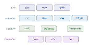
Tactics are commands that transform proof goals. Each tactic takes the current goal and produces zero or more subgoals. A proof is complete when no goals remain.
Definition 6 (Tactic).
A tactic is a function that transforms a proof obligation into a (possibly empty) list of simpler obligations. A proof is a sequence of tactics such that the composition reduces the initial goal to the empty list.
We now survey the most important tactics with examples.
intro.
Introduces a hypothesis or universally quantified variable.
-- Goal: forall n : Nat, n = n
-- After 'intro n': Goal becomes n = n with n : Nat in context
exact.
Provides the exact proof term for the current goal.
-- Goal: P Context: h : P
-- 'exact h' closes the goal
apply.
Applies a function or lemma to the goal, generating subgoals for its arguments.
-- Goal: Q Context: h : P -> Q
-- 'apply h' changes goal to P
rw (rewrite).
Rewrites the goal using an equality.
-- Goal: a + 0 = a
-- 'rw [Nat.add_zero]' rewrites to a = a, then rfl closes it
simp.
The simplifier: applies a collection of rewrite rules repeatedly until no
more apply. Lean ships with hundreds of @[simp] lemmas.
-- simp can solve: 0 + n = n, n * 1 = n, True / P <-> P, etc.
example (n : Nat) : 0 + n = n := by simp
ring.
Proves equalities in commutative (semi)rings by normalisation.
example (a b : Int) : (a + b) ^ 2 = a ^ 2 + 2 * a * b + b ^ 2 := by
ring
omega.
Decides linear arithmetic over natural numbers and integers.
example (n m : Nat) (h : n < m) : n + 1 <= m := by omega
cases.
Performs case analysis on an inductive type.
theorem zero_or_succ (n : Nat) : n = 0 \/ exists m, n = m + 1 := by
cases n with
| zero => left; rfl
| succ m => right; exact <m, rfl>
induction.
Performs structural induction on an inductive type.
constructor.
Applies the constructor of an inductive type to split a goal.
-- Goal: P / Q
-- 'constructor' splits into two goals: P and Q
have.
Introduces an intermediate result (a local lemma).
-- 'have h : P := proof_of_P' adds h : P to the context
calc.
Writes a calculation-style proof as a chain of equalities or inequalities.
example (a b c : Nat) (h1 : a = b) (h2 : b = c) : a = c := by
calc a = b := h1
_ = c := h2
Dependent Types
The real power of Lean comes from dependent types: types that depend on values.
Definition 7 (Dependent Function Type (Pi Type)).
Given a type and a family , the dependent function type (Pi type) is: A term is a function that, given , returns a term of type . When does not depend on , this reduces to the ordinary function type .
Definition 8 (Dependent Pair Type (Sigma Type)).
Given and , the dependent pair type (Sigma type) is: A term is a pair where and . This is the type-theoretic existential quantifier.
Example 14 (Length-Indexed Vectors).
A vector of length is a list whose type encodes its length:
inductive Vec (A : Type) : Nat -> Type where
| nil : Vec A 0
| cons : A -> Vec A n -> Vec A (n + 1)
Vec Nat 3 contains exactly lists of three natural numbers.
Lean's type checker statically rejects any attempt to, say,
concatenate a Vec A n and a Vec A m and claim the result
has type Vec A (n + m + 1).Example 15 (Safe Head).
With dependent types, we can write a head function that is
total: it can never fail at runtime because the type system
guarantees the vector is non-empty.
def Vec.head : Vec A (n + 1) -> A
| .cons a _ => a
nil case is needed because Lean's pattern exhaustiveness
checker knows that Vec A (n + 1) cannot be nil.Structures and Typeclasses
Lean organises mathematical abstractions using typeclasses, a mechanism borrowed from Haskell but extended with dependent types.
class Group (G : Type) extends Mul G, One G, Inv G where
mul_assoc : forall a b c : G, a * b * c = a * (b * c)
one_mul : forall a : G, 1 * a = a
inv_mul : forall a : G, a^(-1) * a = 1
Remark 6.
The extends keyword creates a hierarchy: Group extends
Mul, One, and Inv. Lean's typeclass inference
automatically finds instances, so a theorem about groups applies to any
type with a Group instance (integers, permutations, matrices,
etc.) without the user specifying which instance to use.
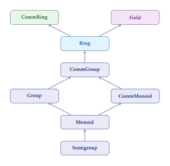
Group automatically applies to CommGroup,
Ring, CommRing, and Field.Example 16 (Using Typeclasses).
-- This theorem works for ANY group, not just a specific one
theorem mul_right_cancel [Group G] (a b c : G)
(h : a * c = b * c) : a = b := by
have : a * c * c^(-1) = b * c * c^(-1) := by rw [h]
simp [mul_assoc, mul_inv_cancel] at this
exact this
[Group G] notation tells Lean to find a Group
instance for G automatically.The Three Axioms
Lean 4's kernel is constructive, but Lean adds three axioms to support classical mathematics:
Propositional extensionality: if then .
axiom propext : (P <-> Q) -> P = QQuotient types: given an equivalence relation on a type, form the type of equivalence classes.
Choice: for any non-empty type, there exists a choice function.
axiom Classical.choice : Nonempty A -> A
Caution.
The axiom of choice makes Lean non-constructive: proofs using
Classical.choice do not compute. This is acceptable for
formalising classical mathematics but means some proofs cannot be
“run” as programs.
Insight.
From choice, Lean derives the law of excluded middle () and proof by contradiction. This means Lean supports the full power of classical reasoning while keeping the kernel constructive.
What Cannot Be Formalised?
A natural question arises: can everything be formalised in Lean?
Theorem 4 (Gödel's First Incompleteness Theorem, Informal).
Any consistent formal system capable of expressing basic arithmetic contains statements that are true but unprovable within .
Remark 7.
This means Lean, if consistent, has true mathematical statements that cannot be proved in Lean. However, this is a theoretical limitation, not a practical one. The “Gödel sentences” are self-referential and do not arise in ordinary mathematics. In practice, Lean can formalise essentially all of known mathematics, as demonstrated by Mathlib's coverage of thousands of theorems across algebra, analysis, topology, number theory, and combinatorics.
Key Idea.
Gödel's theorem does not prevent Lean from being useful; it prevents Lean from being complete. The distinction matters: a system can be enormously powerful without proving every truth.
Exercises
Exercise 15.
Write a Lean 4 proof of using
the induction tactic.
Exercise 16.
Prove
in Lean 4 using only intro, cases, constructor,
and exact.
Exercise 17.
Define an inductive type BinTree of binary trees with natural
number labels. Write a function sum : BinTree → Nat that
computes the sum of all labels, and prove that the sum of a single-node
tree with label equals .
Exercise 18.
Prove the contrapositive: in
Lean 4. Then prove the converse using Classical.em
(excluded middle).
Exercise 19.
(Challenge.) Define a length-indexed vector type and prove that
Vec.append satisfies
at the type level (i.e., the type of append encodes this
property).
Lean 4 by Example
We now work through extended examples that demonstrate how real mathematics is formalised in Lean 4. Each example builds on the foundations from Introduction to Lean 4, gradually introducing Mathlib and more advanced techniques.
Elementary Number Theory
Example 17 (Divisibility).
In Lean, means :
-- Prove that 3 divides 12
example : 3 | 12 := <4, rfl>
-- Transitivity of divisibility
theorem dvd_trans (a b c : Nat)
(h1 : a | b) (h2 : b | c) : a | c := by
obtain <k, hk> := h1
obtain <m, hm> := h2
exact <k * m, by rw [hm, hk]; ring>
Example 18 (GCD and Bézout's Identity).
Mathlib provides Nat.gcd and proves Bézout's identity:
import Mathlib.Data.Nat.GCD.Basic
-- Bezout: there exist integers a, b such that
-- a * m + b * n = gcd m n
#check Nat.gcd_eq_gcd_ab -- the Bezout lemma in Mathlib
Example 19 (Infinitely Many Primes (Euclid's Theorem)).
This is one of the most elegant proofs in mathematics. We prove it step by step in Lean, following Euclid's original argument.
The key idea: given any finite list of primes , the number is not divisible by any , so it has a prime factor not in the list.
import Mathlib.Data.Nat.Prime.Basic
-- Euclid's theorem: for every n, there exists a prime > n
theorem exists_infinite_primes (n : Nat) :
exists p, n < p / Nat.Prime p := by
-- Consider n! + 1
let N := Nat.factorial n + 1
-- N >= 2, so it has a prime factor
have hN : 2 <= N := by omega
obtain <p, hp_prime, hp_dvd> := Nat.exists_prime_and_dvd
(by omega : N != 1)
use p
constructor
* -- Show p > n
by_contra h
push_neg at h
-- p <= n, so p divides n!
have : p | Nat.factorial n :=
hp_prime.dvd_factorial.mpr h
-- p divides N and n!, so p divides N - n! = 1
have : p | 1 := by
have := Nat.dvd_sub' hp_dvd this
simp at this; exact this
-- But p >= 2, contradiction
exact Nat.Prime.one_lt hp_prime |>.not_le
(Nat.le_of_dvd one_pos this)
* exact hp_prime
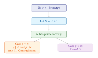
Real Analysis
Lean's Mathlib library formalises real analysis using filters, an elegant abstraction that unifies limits of sequences, functions, and topological convergence.
Definition 9 (Convergence via Filters).
A sequence converges to if for every neighbourhood of , there exists such that for all . In Lean:
-- Filter.Tendsto f atTop (nhds L)
-- means: f(n) -> L as n -> infinity
Example 20 (Proving ).
import Mathlib.Analysis.SpecificLimits.Basic
example : Filter.Tendsto (fun n : Nat => (1 : Real) / n)
Filter.atTop (nhds 0) := by
exact tendsto_const_div_atTop_nhds_0_nat 1
Example 21 (The Squeeze Theorem).
-- If a_n <= b_n <= c_n and a_n -> L and c_n -> L, then b_n -> L
theorem squeeze_theorem
{a b c : Nat -> Real} {L : Real}
(hab : forall n, a n <= b n)
(hbc : forall n, b n <= c n)
(ha : Filter.Tendsto a Filter.atTop (nhds L))
(hc : Filter.Tendsto c Filter.atTop (nhds L)) :
Filter.Tendsto b Filter.atTop (nhds L) := by
apply tendsto_of_tendsto_of_tendsto_of_le_of_le ha hc
* exact eventually_of_forall hab
* exact eventually_of_forall hbc
Linear Algebra
Example 22 (Vector Spaces in Mathlib).
Mathlib uses the typeclass Module to represent vector spaces
(a module over a field):
import Mathlib.LinearAlgebra.Basic
-- R-module structure provides:
-- * Addition: v + w
-- * Scalar multiplication: r * v
-- * Module axioms (distributivity, associativity, etc.)
-- Example: R^n as a module
example : Module Real (Fin 3 -> Real) := inferInstance
Example 23 (Linear Maps).
-- A linear map preserves addition and scalar multiplication
-- LinearMap R M N is the type of R-linear maps from M to N
-- The kernel of a linear map
#check LinearMap.ker -- Submodule R M
-- The rank-nullity theorem
#check LinearMap.finrank_range_add_finrank_ker
-- : finrank (range f) + finrank (ker f) = finrank M
Group Theory
Example 24 (Subgroups and Lagrange's Theorem).
import Mathlib.GroupTheory.Lagrange
-- Lagrange's theorem: |H| divides |G|
#check Subgroup.card_subgroup_dvd_card
-- : card H | card G
-- A consequence: the order of an element divides |G|
#check orderOf_dvd_card
Working with Mathlib
Key Idea.
Mathlib is the world's largest library of formalised mathematics, containing over 210,000 theorems and 100,000 definitions across nearly 2 million lines of Lean 4 code. It covers algebra, analysis, topology, number theory, combinatorics, measure theory, probability, and category theory.
Searching for lemmas.
Lean 4 provides several tactics for discovering relevant lemmas:
-- exact? : searches for a single lemma that closes the goal
-- apply? : searches for a lemma whose conclusion matches the goal
-- simp? : runs simp and reports which lemmas were used
-- rw? : searches for a rewrite rule
example (n : Nat) (h : n > 0) : n != 0 := by
exact? -- suggests: exact Nat.pos_iff_ne_zero.mp h
Remark 8.
These search tactics are invaluable for both human and AI provers. Neural theorem provers like ReProver use retrieval-augmented generation to replicate this search at scale, finding relevant premises from the entire Mathlib library.
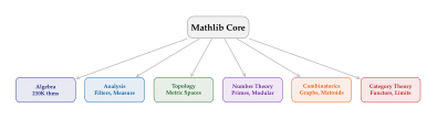
Common Pitfalls and Debugging
Caution.
The following are the most common errors encountered when learning Lean 4, and exactly the errors that AI systems must learn to avoid or recover from.
Universe errors.
Lean's universe polymorphism can produce confusing errors:
-- ERROR: universe level mismatch
-- This often occurs when mixing Prop and Type
-- Fix: use 'universe u' declarations or explicit annotations
Typeclass inference failures.
When Lean cannot find an instance:
-- ERROR: failed to synthesize instance
-- CommRing (Matrix (Fin 2) (Fin 2) Nat)
-- Fix: ensure the right imports and instance declarations
Definitional vs. propositional equality.
-- 2 + 2 = 4 is DEFINITIONAL (rfl works)
-- n + 0 = n is PROPOSITIONAL (requires induction proof)
-- This distinction trips up beginners and AI models alike
Insight.
Understanding which equalities are definitional (solved by rfl)
versus propositional (requiring explicit proof) is one of the most
important skills in Lean programming. Neural theorem provers that
learn this distinction achieve significantly higher success rates.
A Complete Worked Example: The Irrationality of
We conclude with a complete, annotated proof of a classical result.
Theorem 5.
is irrational.
Proof Strategy.
Suppose with coprime. Then , so is even, say . Then , so , making even. This contradicts .
import Mathlib.Data.Rat.Sqrt
import Mathlib.Data.Int.Parity
theorem sqrt_two_irrational : Irrational (Real.sqrt 2) := by
rw [irrational_sqrt_two]
-- Mathlib already has this! But let us sketch the structure:
-- 1. Assume sqrt 2 = p / q, coprime
-- 2. Then 2 * q^2 = p^2
-- 3. p^2 even => p even => p = 2k
-- 4. 2 * q^2 = 4 * k^2 => q^2 = 2 * k^2
-- 5. q^2 even => q even
-- 6. Contradiction with coprimality
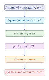
The Compilation Pipeline and Performance
Lean 4 is unique among theorem provers in being a compiled language.
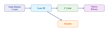
Remark 9.
The compilation pipeline means Lean 4 programs run at near-native speed. This matters for AI: proof search algorithms implemented in Lean can run efficiently, and tactics can perform complex computations during type-checking. The self-hosted compiler (Lean compiles itself) is a testament to the language's maturity.
Further Exercises
Exercise 20.
Prove in Lean 4 that the sum of the first natural numbers is
. Hint: use induction and ring.
Exercise 21.
Formalise the definition of a metric space in Lean 4 as a structure with fields for the distance function and the metric axioms (non-negativity, identity of indiscernibles, symmetry, triangle inequality). Prove that with the absolute value distance is an instance.
Exercise 22.
(Challenge.) Using Mathlib, prove that every finite group of
prime order is cyclic. Hint: search for
IsCyclic.of_prime_card in Mathlib.
Exercise 23.
Write a Lean 4 function that computes the Fibonacci sequence, and prove that for all .
Exercise 24.
(Research.) Use the exact? and apply? tactics
to find a Mathlib proof that every continuous function on is
bounded. Write down the chain of lemmas involved and explain how a
neural theorem prover might discover this chain.
Lean 4 Advanced Topics and Practical Formalization
The preceding sections introduced Lean 4 as a language and sketched its role in the AI-for-mathematics pipeline. We now dive substantially deeper. Our goals in this section are threefold: (1) to explain the dependent type theory that makes Lean 4 expressive enough to state any theorem in mathematics; (2) to survey the tactic language that makes proving those theorems feasible; and (3) to walk through two extended worked examples that show what real formalization looks like in practice.
Readers who have never touched a proof assistant may find the first subsection challenging. We encourage persistence: the payoff is a precise understanding of what it means for a computer to verify a mathematical argument, and that understanding is essential for appreciating the generative models discussed in the remainder of this chapter.
Key Idea.
Lean 4's power as a proof assistant derives from the Calculus of Inductive Constructions (CIC), a dependent type theory in which propositions are types and proofs are terms. Every Lean 4 proof is a well-typed program, and the type-checker is the ultimate arbiter of correctness.
Dependent Types in Depth
In a simply-typed language such as Haskell or OCaml, the type of a function can depend on other types (polymorphism), but it cannot depend on values. Dependent type theory removes this restriction: types may mention ordinary terms. The canonical first example is a vector of known length.
Definition 10 (Length-Indexed Vector).
In Lean 4, a vector of length carrying elements of type is defined as an inductive type whose constructors enforce the length invariant at the type level:
inductive Vec (alpha : Type) : Nat -> Type where
| nil : Vec alpha 0
| cons : alpha -> Vec alpha n -> Vec alpha (n + 1)
Vec \(\) n depends on the value
. A function
Vec.append : Vec \(\) m \(\) Vec \(\) n
\(\) Vec \(\) (m + n) can state in its type signature
that the output length is exactly the sum of the input lengths.
The type-checker verifies this at compile time.Why does this matter for formalization? Because mathematical objects often carry constraints that are part of their identity. A matrix in has rows and columns; a permutation on has exactly elements; a probability distribution over a finite set sums to one. Dependent types let us encode these constraints directly in the type, so that ill-formed objects are not merely flagged at runtime but are literally impossible to construct.
Example 25.
Matrices with dimensions in the type. Mathlib defines matrices as functions from a row index set to a column index set:
def Matrix (m n : Type) (alpha : Type) := m -> n -> alpha
Fin 3 for the
set ), the dimensions are encoded in the type.
Matrix multiplication
def Matrix.mul [Fintype n] [Mul alpha] [AddCommMonoid alpha]
(A : Matrix m n alpha) (B : Matrix n p alpha) : Matrix m p alpha :=
fun i k => sum j, A i j * B j k
More generally, a dependent function type (also called a
Pi-type) has the form
where is a family of types indexed by elements of . In
Lean 4 syntax this is written (x : A) \(\) B x.
When does not actually depend on , the Pi-type reduces to
the ordinary function type . At the other extreme,
when is Prop and maps each proposition to its
proof type, the Pi-type encodes universal quantification:
“for all , holds” is precisely
.
The dual notion is the Sigma-type , which packages a value together with a witness of type . This encodes existential quantification: “there exists such that holds” becomes .
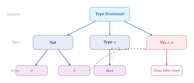
Vec $$ 3, ensuring at compile time that the
vector has exactly three elements. In a simply-typed language,
no such dependency exists: the type level and value level are
strictly separated.Inductive Types and Pattern Matching
Lean 4 follows the tradition of Martin-Löf type theory in building complex data types from inductive definitions. An inductive type is specified by listing its constructors, each of which may take arguments, including recursive references to the type being defined. The canonical example is the natural numbers.
inductive Nat where
| zero : Nat
| succ : Nat -> Nat
This says: a natural number is either zero or the
successor of another natural number. From this single
definition, Lean derives an induction principle, a recursion
principle, and decidable equality. Pattern matching on the
constructors gives us structural recursion:
def add : Nat -> Nat -> Nat
| m, .zero => m
| m, .succ n => .succ (add m n)
The termination checker verifies that the recursive call
add m n decreases on the second argument, ensuring that
the function is total.
Lists, binary trees, and abstract syntax trees all follow the same pattern:
inductive List (alpha : Type) where
| nil : List alpha
| cons : alpha -> List alpha -> List alpha
inductive BinTree (alpha : Type) where
| leaf : BinTree alpha
| branch : BinTree alpha -> alpha -> BinTree alpha -> BinTree alpha
For formalization, the most important inductive types are the propositions. In Lean 4, the logical connectives are themselves inductively defined:
-- Conjunction (already in core)
structure And (a b : Prop) : Prop where
intro ::
left : a
right : b
-- Disjunction (already in core)
inductive Or (a b : Prop) : Prop where
| inl : a -> Or a b
| inr : b -> Or a b
A proof of is a pair of proofs (one for , one for ); a proof of is either a proof of or a proof of , tagged to say which case holds. This is the Curry–Howard correspondence made concrete: logical connectives are type constructors, and proofs are data.
Remark 10.
Custom inductive types are ubiquitous in formalization. For
example, Mathlib defines a type SimpleGraph to
represent simple undirected graphs, with constructors that
enforce the absence of self-loops and the symmetry of the
adjacency relation. Any theorem proved about
SimpleGraph automatically inherits these invariants
because they are baked into the type.
Tactics in Depth
A tactic in Lean 4 is a metaprogram that transforms the current proof state (a list of goals, each consisting of a local context and a target type) into a new proof state with fewer or simpler goals. When no goals remain, the proof is complete. Lean 4 ships with a rich library of built-in tactics, and Mathlib adds many more. We survey the most important ones.
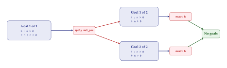
apply mul_pos splits one
goal into two subgoals, each of which is closed by
exact h. When no goals remain, Lean assembles the
underlying proof term automatically.The simp Tactic and the Simp Lemmas Database
The simp tactic is the workhorse of Lean 4
formalization. It applies a configurable set of rewrite rules
(called simp lemmas) to simplify the goal. A simp lemma
is any lemma tagged with the @[simp] attribute; Mathlib
contains thousands of such lemmas.
@[simp] theorem Nat.add_zero (n : Nat) : n + 0 = n := ...
@[simp] theorem List.length_nil : [].length = 0 := ...
@[simp] theorem Bool.not_not (b : Bool) : !!b = b := ...
When invoked, simp repeatedly applies matching simp
lemmas until no further simplification is possible. It can also
unfold definitions, apply congruence rules, and use hypotheses
from the local context:
example (n : Nat) : n + 0 + 0 = n := by simp
example (xs : List alpha) : (xs ++ []).length = xs.length := by simp
example (h : a = b) : a + c = b + c := by simp [h]
The variant simp only [lemma1, lemma2] restricts
simplification to an explicit list of lemmas, which is useful
when the full simp set produces undesirable results or when
performance matters.
Remark 11.
The simp lemma database is a double-edged sword. Adding too many
simp lemmas can cause simplification loops (where rewrites to
and rewrites to ) or exponential blowup. Mathlib
maintainers carefully curate the @[simp] attribute,
and contributors are expected to justify each new simp lemma.
This curation effort is one of the less visible but most
important aspects of large-scale formalization.
The omega Tactic
The omega tactic decides the theory of linear arithmetic
over the integers and natural numbers. It can prove any
goal that is a Boolean combination of linear inequalities and
equalities:
example (n m : Nat) (h : n < m) : n + 1 <= m := by omega
example (a b : Int) (h1 : a <= b) (h2 : b <= a) : a = b := by omega
example (x : Nat) : x / 2 + x / 2 + x
Under the hood, omega implements the Omega test of
Pugh [76], which decides Presburger
arithmetic by quantifier elimination. The implementation in
Lean 4 is a verified decision procedure: the tactic produces a
proof term that the kernel can check, so the correctness of
omega does not enlarge the trusted computing base.
The ring Tactic
The ring tactic proves equalities in commutative
(semi)rings by normalizing both sides to a canonical form (a sum
of monomials sorted lexicographically) and checking syntactic
equality:
example (a b : Int) : (a + b)^2 = a^2 + 2*a*b + b^2 := by ring
example (x y z : Rat) : x*(y+z) - x*y - x*z = 0 := by ring
example (n : Nat) : n*(n+1)/2 + (n+1) = (n+1)*(n+2)/2 := by ring
The ring tactic works for any type that is an instance of
the CommRing (or CommSemiring) type class.
This includes integers, rationals, reals, complex numbers, and
polynomials.
The norm_num Tactic
The norm_num tactic evaluates numerical expressions and
proves numerical facts:
example : (7 : Nat) * 13 = 91 := by norm_num
example : (2 : Real)^10 = 1024 := by norm_num
example : Nat.Prime 104729 := by norm_num
example : Not Nat.Prime 91 := by norm_num
Beyond simple arithmetic, norm_num supports an
extensible plugin system: Mathlib registers plugins for
primality testing, divisibility checks, modular arithmetic,
and more. Each plugin produces a verified proof certificate,
so the kernel trusts only its own type-checking, not the
plugin's computation.
The polyrith Tactic
The polyrith tactic proves polynomial arithmetic goals
by calling an external oracle (typically a Gröbner basis
computation via SageMath or a similar system) to find a
certificate, then verifying the certificate within Lean:
example (a b c : Rat) (h1 : a + b + c = 0) (h2 : a*b + b*c + a*c = -1) :
a^2 + b^2 + c^2 = 2 := by polyrith
This is a powerful example of the oracle pattern: the hard computational work (finding the certificate) is done by an untrusted external tool, while the easy verification work (checking the certificate) is done by the trusted kernel. The correctness of the overall proof depends only on the kernel, not on SageMath.
The aesop Tactic
The aesop tactic (Automated Extensible Search for
Obvious Proofs) performs a best-first tree search over a
configurable set of rules. It can apply lemmas, introduction
rules, elimination rules, simp lemmas, and custom user-defined
rules. It is particularly effective for closing goals that
require a combination of case splitting, simplification, and
hypothesis application:
example (h : a in s union t) (hs : s subset u) (ht : t subset u) : a in u := by aesop
Mathlib tags many lemmas with @[aesop safe],
@[aesop unsafe 50%], etc., to guide aesop's search.
The percentages indicate the tactic's confidence that a rule will
be useful, influencing the search priority.
Example 26.
Aesop in action. Consider proving that the intersection distributes over union for finite sets. The goal
example (x : alpha) (s t u : Set alpha) (h : x in s inter (t union u)) :
x in (s inter t) union (s inter u) := by aesop
aesop in a single invocation. Internally,
aesop decomposes the membership hypothesis, performs case analysis
on the union, and applies the introduction rules for intersection
and union membership. The trace (visible with
set_option trace.aesop true) shows the search tree:
aesop first tries safe rules (like And.intro), then
falls back to unsafe rules (like case-splitting on Or)
when safe rules alone do not close the goal. Understanding
this trace is invaluable when aesop fails: the trace reveals
which subgoals remain open, guiding the user toward the missing
lemma or hypothesis.The decide Tactic
The decide tactic works on propositions for which
Lean can find an instance of Decidable P. It evaluates
the decision procedure and, if the result is true,
extracts a proof:
example : 2 + 3 = 5 := by decide
example : Not (3 | 7) := by decide
example : Finset.card {1, 2, 3, 4, 5} = 5 := by decide
The decide tactic is conceptually simple but can be
slow for large computations because it runs the decision
procedure inside the kernel. For numerical facts,
norm_num is almost always faster because it produces
compact proof certificates rather than evaluating step by step.
Key Idea.
The tactic ecosystem in Lean 4 forms a spectrum from
surgical tactics (exact, apply,
intro) that make a single logical step, through
domain-specific decision procedures (omega,
ring, norm_num) that handle specific
theories, to general-purpose search tactics
(simp, aesop) that combine many rules.
Effective formalization requires knowing when to use each.
Writing Custom Tactics
Because Lean 4 is a general-purpose programming language, its
tactic framework is not a separate language bolted on top: it is
ordinary Lean code that manipulates proof states. A tactic is a
function of type TacticM Unit, where TacticM is
a monad that provides access to the current goal, the local
context, and the ability to create new metavariables.
The simplest custom tactic is one that wraps existing tactics with additional logic:
/-- A tactic that tries `simp`, then `omega`, then `ring`. -/
syntax "auto_close" : tactic
macro_rules
| `(tactic| auto_close) =>
`(tactic| first | simp | omega | ring)
More sophisticated tactics can inspect the goal, pattern-match on its structure, and decide which strategy to use:
elab "smart_arith" : tactic => do
let goal <- Lean.Elab.Tactic.getMainTarget
if goal.isAppOf ``Eq then
-- Try ring for equalities
Lean.Elab.Tactic.evalTactic (<- `(tactic| ring))
else
-- Try omega for inequalities
Lean.Elab.Tactic.evalTactic (<- `(tactic| omega))
This ability to program new tactics is what makes Lean 4 uniquely suited to AI-driven formalization: a generative model can output not only proofs but also custom tactics that encode proof strategies [9].
Metaprogramming in Lean 4
Lean 4's metaprogramming framework operates at three levels, each offering increasing power and complexity.
Syntax extensions and notations.
Lean 4 allows users to define new syntax using the
syntax, notation, and macro commands.
For example, Mathlib defines the notation
as:
notation "sum" i " in " s ", " f => Finset.sum s (fun i => f)
Macros.
A macro is a syntax transformation that runs before elaboration. Macros can pattern-match on syntax objects and produce new syntax:
macro "square" x:term : term => `($x * $x)
#eval square 7 -- outputs 49
Elaboration-time metaprogramming.
For full control, users can write elaborators: Lean functions that run during type-checking and can inspect the environment, create metavariables, unify types, and build terms. This is the mechanism used to implement tactics, derive handlers, and the entirety of the tactic mode.
The elaboration pipeline proceeds in stages:
Parsing: source text is converted to a concrete syntax tree (CST).
Macro expansion: macros are expanded until no more macros apply.
Elaboration: the CST is converted to a fully-typed core expression, with metavariables for missing information.
Type inference and unification: metavariables are solved by unification constraints.
Kernel type-checking: the final expression is checked by the trusted kernel.
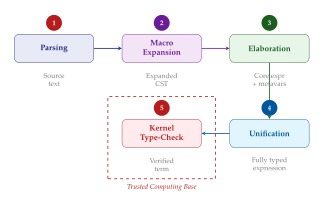
Worked Example: Formalizing the Bolzano–Weierstrass Theorem
We now present a detailed worked example that illustrates the full workflow of formalizing a nontrivial result in real analysis. We chose the Bolzano–Weierstrass theorem because it is well-known, conceptually rich, and exercises several features of Lean 4 and Mathlib simultaneously.
The Informal Statement and Proof
Theorem 6 (Bolzano–Weierstrass).
Every bounded sequence of real numbers has a convergent subsequence.
Informal proof.
Let be a bounded sequence, so there exist with for all . We construct a convergent subsequence by the method of nested intervals.
Set . At each stage , we bisect the interval into and , where . At least one of these halves contains infinitely many terms of the sequence (because the full interval does). We choose a half that contains infinitely many terms and call it . We also pick an index such that .
The sequences and are monotone and bounded, so they converge. Moreover, , so they converge to the same limit, say . By the squeeze theorem, .
Setting Up the Lean Formalization
The first task is to identify the relevant Mathlib concepts. In
Mathlib, a sequence of reals is simply a function
. Boundedness is expressed via
the predicate Bornology.IsBounded or equivalently by
asserting that the range of lies in some interval. A
subsequence is encoded using a strictly increasing function
, and the subsequence
itself is . Convergence is expressed via the
filter Filter.Tendsto.
import Mathlib.Topology.Sequences
import Mathlib.Topology.MetricSpace.Basic
import Mathlib.Topology.Order.Basic
open Filter Topology
The Formal Statement
The Bolzano–Weierstrass theorem already exists in Mathlib as
IsCompact.tendsto_subseq, which states that a sequence
in a compact set has a convergent subsequence. For pedagogical
purposes, we specialize this to the real numbers:
theorem bolzano_weierstrass
(a : Nat -> Real)
(hbdd : exists M : Real, forall n, |a n| <= M) :
exists (phi : Nat -> Nat), StrictMono phi /
exists (l : Real), Tendsto (a o phi) atTop (nhds l) := by
sorry -- to be filled in
Let us unpack the statement. The hypothesis hbdd says
that there exists a bound such that for all
. The conclusion asserts the existence of a strictly
increasing function (the subsequence indices) and a
limit such that converges to in
the neighborhood filter .
Walking Through the Proof
The proof strategy in Lean mirrors the informal proof but uses the more general Mathlib machinery of compact sets:
theorem bolzano_weierstrass
(a : Nat -> Real)
(hbdd : exists M : Real, forall n, |a n| <= M) :
exists (phi : Nat -> Nat), StrictMono phi /
exists (l : Real), Tendsto (a o phi) atTop (nhds l) := by
-- Step 1: Extract the bound M
obtain <M, hM> := hbdd
-- Step 2: The range of a lies in the closed ball [-M, M]
have hrange : forall n, a n in Set.Icc (-M) M := by
intro n
constructor
* linarith [abs_le.mp (hM n)]
* linarith [abs_le.mp (hM n)]
-- Step 3: The closed interval [-M, M] is compact
have hcpt : IsCompact (Set.Icc (-M) M) :=
isCompact_Icc
-- Step 4: Apply the sequential compactness theorem
obtain <l, hlmem, phi, hphimono, hphitend> :=
hcpt.tendsto_subseq hrange
-- Step 5: Package the result
exact <phi, hphimono, l, hphitend>
Let us examine each step:
Step 1 (
obtain): Destructs the existential hypothesis to get a concrete and a proofhMthat for all .Step 2 (
have): Shows that each lies in . The key Mathlib lemmaabs_leconverts into . Thelinarithtactic handles the linear arithmetic.Step 3 (
have): Appeals to the Mathlib lemmaisCompact_Icc, which states that closed bounded intervals in are compact. This is where the Heine–Borel theorem is hiding.Step 4 (
obtain): This is the core step. The lemmaIsCompact.tendsto_subseqstates that if is compact and for all , then there exist , a strictly increasing , and a proof that .Step 5 (
exact): Repackages the extracted data into the form required by the goal.
Remark 12.
The formal proof is notably shorter than the informal proof
because it delegates the hard work (the construction of the
subsequence via nested intervals) to Mathlib's
tendsto_subseq. This is typical: formalization
rewards building on libraries rather than reproving
everything from scratch. Identifying the right Mathlib lemma
to appeal to is often the hardest part of a formalization, and
it is precisely this search task that generative models can
assist with.
Worked Example: Formalizing Lagrange's Theorem
Our second worked example comes from algebra. Lagrange's theorem is one of the first nontrivial results in group theory.
Theorem 7 (Lagrange).
If is a finite group and is a subgroup of , then the order of divides the order of .
Informal Proof Sketch
The key idea is to partition into left cosets of : the sets for each . The cosets are pairwise disjoint and each has exactly elements (because the map is a bijection ). Since is the disjoint union of its cosets, so divides .
The Lean Formalization
In Mathlib, finite groups are modeled using the Fintype
type class, and subgroups are terms of type Subgroup G.
The cardinality of a finite type is Fintype.card.
Lagrange's theorem is already proved in Mathlib:
import Mathlib.GroupTheory.Coset
import Mathlib.GroupTheory.Index
variable {G : Type*} [Group G] [Fintype G]
(H : Subgroup G) [Fintype H]
-- The Mathlib statement:
-- Subgroup.card_subgroup_dvd_card : Fintype.card H | Fintype.card G
-- We can also state it ourselves and prove it from Mathlib:
theorem lagrange :
Fintype.card H | Fintype.card G := by
exact Subgroup.card_subgroup_dvd_card H
While the one-line proof is anticlimactic, the point is that
Mathlib has already done the heavy lifting. Let us examine
what lies beneath card_subgroup_dvd_card. The proof
chain involves:
The quotient (the set of left cosets) is a
Fintype.There is a bijection between and (the coset partition).
The cardinality of a product type is the product of the cardinalities.
Therefore , and .
If we want to see more of the proof structure, we can unfold one layer:
theorem lagrange_detailed :
Fintype.card H | Fintype.card G := by
rw [Subgroup.card_eq_card_quotient_mul_card_subgroup]
exact dvd_mul_left (Fintype.card H) (Fintype.card (G / H))
Here, card_eq_card_quotient_mul_card_subgroup is
the key identity , and
dvd_mul_left witnesses that divides
.
Lessons from the Two Examples
Both worked examples illustrate a common pattern in modern formalization. The informal mathematical argument is restructured to match the abstractions available in the library. In the Bolzano–Weierstrass example, we did not implement the nested-intervals construction; instead, we recognized that the key abstraction is compactness and appealed to a general theorem about compact sets. In the Lagrange example, we did not construct the coset partition; instead, we appealed to a theorem about the cardinality of quotient types.
This pattern has a direct implication for AI: a generative model that can map informal proof strategies to the right library abstractions will produce short, elegant formalizations. A model that tries to translate informal proofs literally will produce verbose, brittle code that duplicates existing library content. The ability to search the library effectively is therefore at least as important as the ability to generate tactic sequences [9].
Remark 13.
The gap between informal and formal proof is sometimes called the formalization gap. It is not merely a matter of adding detail; it often requires reconceptualizing the proof in terms of the available formal infrastructure. This reconceptualization is a creative act, and it is one of the most challenging aspects of formalization for both humans and AI systems.
Performance and Compilation
Lean 4 compiles to native code via C, and its compiler is designed to handle large libraries efficiently. Several design choices contribute to performance:
Incremental compilation.
Lean 4 uses a file-level incremental compilation model: each
.lean file is compiled independently, and only files
whose dependencies have changed are recompiled. This is crucial
for Mathlib, which consists of over 4,000 files totaling
more than one million lines of code.
Reference counting.
Instead of garbage collection, Lean 4 uses reference counting with a “reset–reuse” optimization: when the last reference to an object is consumed, the memory is reused in place rather than freed and reallocated. This makes functional programming competitive with imperative code for many workloads.
Lazy evaluation of proofs.
Lean 4 does not evaluate proof terms during compilation (proofs are erased from the compiled output). This means that a file can import thousands of theorems without paying any runtime cost for the proofs; only the types (statements) are retained.
Parallel checking.
The Lean 4 server supports parallel elaboration: different declarations within a file can be type-checked concurrently. On modern hardware with many cores, this significantly reduces the wall-clock time for checking large files.
Example 27.
Mathlib compilation.
As of 2024, building Mathlib from scratch takes approximately
two to three hours on a machine with 16 cores and 64 GB of
RAM. Incremental builds after a small change typically complete
in under a minute. The compiled .olean files (Lean's
binary format for compiled declarations) total roughly 2 GB on
disk. These precompiled files can be downloaded via
lake exe cache get, so that most users never need to
build Mathlib from source [14].
Exercises for Section 6
Exercise 25.
Define a dependently-typed function
Vec.zip : Vec \(\) n \(\) Vec \(\) n
\(\) Vec (\( \)) n
that pairs up corresponding elements of two vectors of the same
length. Explain why the type signature guarantees that the
inputs have the same length and the output also has that length.
Write out the definition using pattern matching and verify
(informally or in Lean) that it type-checks.
Exercise 26.
For each of the following goals, identify which Lean 4 tactic would close the goal most directly. Justify your choice.
where .
where .
.
where .
where are sets.
Exercise 27.
Write a Lean 4 macro contrapose that transforms a goal
of the form into . (Hint: use
macro_rules to expand to
intro h; exact Classical.not_imp_not.mpr (fun hq => h),
or use an appropriate Mathlib tactic.) Test your macro on two
examples.
Exercise 28.
In the worked example of the Bolzano–Weierstrass theorem
(Worked Example: Formalizing the Bolzano–Weierstrass Theorem), we used
IsCompact.tendsto_subseq to avoid constructing the
subsequence explicitly. Outline (in pseudocode or informal
mathematics) the construction that Mathlib uses internally.
What is the role of the axiom of choice in this construction?
Could the theorem be proved constructively?
Exercise 29.
Lagrange's theorem says divides . The quotient is called the index of in , written .
Find the Mathlib name for the index of a subgroup.
State and prove (or find in Mathlib) the identity .
State the tower law: if are subgroups, then . Find its Mathlib proof.
Other Theorem Provers – A Comparative Survey
Lean 4 is the newest entrant in a field with a history stretching back to the 1960s. Understanding the broader landscape of theorem provers is important for three reasons. First, many of the ideas now appearing in Lean (dependent types, tactic languages, large formal libraries) were pioneered in older systems. Second, significant bodies of formalized mathematics exist in systems other than Lean, and AI systems that can work with multiple provers have access to a much larger training corpus. Third, the design choices made by different provers illuminate genuine trade-offs in foundations, automation, and usability.
This section surveys seven major theorem provers, then presents a systematic comparison. We close with a discussion of whether the field is converging on a single system or whether diversity will persist.
Coq (Rocq)
Coq (recently rebranded as Rocq for trademark reasons) is the oldest actively developed proof assistant based on dependent type theory [77]. Development began at INRIA in 1984 under Thierry Coquand and Gérard Huet, with the first public release in 1989. Coq is based on the Calculus of Inductive Constructions (CIC), the same foundation as Lean 4, and for decades it was the de facto standard for constructive formalization.
Key features.
Gallina and Ltac. Coq's specification language is Gallina (a functional language similar to OCaml), and its tactic language is Ltac (or the newer Ltac2). Unlike Lean 4, where tactics and terms live in the same language, Coq maintains a sharper separation between the specification language and the tactic language.
Extraction. Coq can extract verified programs to OCaml, Haskell, or Scheme. This feature has been used to produce verified compilers and verified cryptographic implementations.
Universes. Coq supports a cumulative universe hierarchy with universe polymorphism, similar to Lean 4.
SSReflect.
SSReflect (“Small Scale Reflection”) is a proof methodology and Coq library developed by Georges Gonthier for the formalization of the Four Color Theorem [15]. The key idea is to represent propositions as Boolean computations whenever possible, so that many proof obligations reduce to computation (“reflection”) rather than deduction. SSReflect introduces a distinctive proof style with small, composable tactics and extensive use of Boolean reflection. The Mathematical Components library (MathComp) is the modern incarnation of this approach.
Major achievements.
Four Color Theorem (Gonthier, 2005) [15]: the first formalization of a famous theorem whose original proof relied on computer case analysis.
Odd Order Theorem (Gonthier et al., 2013) [16]: a 150-page proof in algebra, requiring approximately 170,000 lines of Coq code and six years of work.
CompCert (Leroy, 2006) [17]: a verified optimizing C compiler. CompCert's significance extends beyond mathematics: it demonstrated that formal verification could produce software competitive with industrial compilers.
Feit–Thompson Theorem: identical to the Odd Order Theorem, formalized as part of the MathComp project.
Isabelle/HOL
Isabelle is a generic proof assistant framework developed by Lawrence Paulson at Cambridge and Tobias Nipkow at Munich [64]. The most widely used instantiation is Isabelle/HOL, which implements classical higher-order logic (HOL). Unlike Lean and Coq, which are based on dependent type theory, Isabelle/HOL uses a simpler type system (simple type theory with type classes and limited polymorphism) that trades some expressiveness for stronger automation.
Key features.
Sledgehammer. Sledgehammer is Isabelle's flagship automation tool. Given a proof goal, Sledgehammer sends it to one or more external automated theorem provers (E, Vampire, Z3, SPASS) and, if any of them finds a proof, reconstructs the proof within Isabelle using trusted internal methods [18]. Sledgehammer dramatically reduces the manual effort of formalization and is one of the main reasons Isabelle/HOL remains competitive despite its simpler type system.
Isar proof language. Isabelle's structured proof language, Isar (“Intelligible Semi-Automated Reasoning”), produces proofs that read almost like informal mathematics. An Isar proof states intermediate claims with
haveandshow, provides justifications withby, and structures case analysis withconsiderandobtain.Archive of Formal Proofs (AFP). The AFP is a curated, peer-reviewed collection of Isabelle formalizations, containing over 800 entries and millions of lines of code. It functions as a journal of formalized mathematics and computer science.
Major achievements.
Kepler Conjecture (Hales et al., 2017) [19]: the proof that the face-centered cubic packing is the densest sphere packing in three dimensions. The original computer-assisted proof by Hales (1998) was controversial; the Isabelle/HOL formalization (the Flyspeck project) settled the matter definitively.
seL4 (Klein et al., 2009) [20]: a verified microkernel operating system. The proof establishes that the C code of seL4 correctly implements its abstract specification, ruling out entire classes of bugs (buffer overflows, null pointer dereferences, etc.).
Prime Number Theorem (Avigad et al., 2007; Eberl, 2018): formalized within the AFP with full analytic number theory proofs.
Proof style.
An Isabelle/HOL proof in Isar style reads remarkably like informal mathematics. Consider the following proof that the square root of 2 is irrational (sketch):
theorem sqrt2_irrational: "sqrt 2 notin Rat"
proof (rule ccontr)
assume "Not sqrt 2 notin Rat"
then obtain p q :: nat where
"q != 0" and "sqrt 2 = p / q" and "coprime p q"
by (auto simp: Rats_def)
then have "2 * q^2 = p^2"
by (auto simp: power2_eq_square field_simps)
then have "even p" by arith
...
qed
obtain, have, and then keywords
mirror the informal mathematician's habit of introducing
intermediate claims and chaining deductions. This readability
is one of Isabelle's greatest strengths, though it comes at the
cost of more verbose proofs compared to Lean's tactic sequences.
Agda
Agda is a dependently typed programming language and proof assistant developed primarily by Ulf Norell at Chalmers University [78]. Like Lean 4, Agda is based on Martin-Löf type theory (MLTT), but it makes different design choices that give it a distinctive character.
Key features.
No tactics. Agda traditionally does not have a tactic mode. Proofs are written as ordinary programs using pattern matching and recursion. The
Agda.Automodule provides some automation, and recent versions support “auto” and “refine” commands, but the culture remains term-oriented rather than tactic-oriented.Unicode-heavy syntax. Agda embraces Unicode: operators like , , , , and are used directly in source code. Combined with mixfix operators, this makes Agda code visually close to mathematical notation.
Cubical Agda. Cubical Agda extends the language with primitives from cubical type theory, providing a computational interpretation of the univalence axiom from homotopy type theory (HoTT). In cubical Agda, the statement “isomorphic types are equal” is not merely an axiom but a theorem with computational content: transporting a proof along an isomorphism actually computes. This is a feature that no other major proof assistant offers.
Limitations.
Agda's standard library is much smaller than Mathlib, MathComp, or the AFP, which limits its use for large-scale formalization projects. Automation is weaker than in Lean or Isabelle, making proofs more verbose. The community, while passionate, is significantly smaller than Lean's or Coq's.
Contributions.
Agda has been influential in the development of HoTT and as a testbed for advanced type-theoretic features. The HoTT library in Agda contains formalizations of fundamental results in synthetic homotopy theory.
Mizar
Mizar is a proof assistant and a formal language developed by Andrzej Trybulec at the University of Bialystok, with roots going back to 1973 [60]. Mizar takes a fundamentally different approach from the type-theoretic systems: it is based on first-order logic with Tarski–Grothendieck set theory.
Key features.
Natural language style. Mizar proofs are written in a stylized but readable English-like syntax. A typical Mizar proof reads: “Let be a real number. Assume . Then by SQUARE_1:72.” The references (like
SQUARE_1:72) point to specific theorems in the Mizar Mathematical Library (MML).Large formal library. The MML contains over 60,000 theorems and has been under continuous development since the 1980s. It covers a broad range of mathematics, from basic set theory to functional analysis and topology.
Set-theoretic foundation. Unlike type-theoretic systems, Mizar works directly with sets, functions, and first-order logic. This can be more natural for mathematicians trained in the ZFC tradition.
Limitations.
Mizar's tooling is dated compared to Lean, Coq, or Isabelle. It lacks a modern IDE, has limited metaprogramming capabilities, and its community has contracted in recent years. The MML is not easily interoperable with other systems.
Relevance to AI.
Despite its age, Mizar has contributed to AI research through the Mizar Problems for Theorem Proving (MPTP) project, which extracted thousands of proof obligations from the MML and encoded them in first-order TPTP format. These problems have served as benchmarks for automated theorem provers and, more recently, for neural theorem proving systems. The natural-language-like proof format of Mizar has also inspired work on autoformalization: translating informal mathematical text into formal Mizar proofs [79].
HOL Light and HOL4
The HOL family of theorem provers (“Higher Order Logic”) descends from Mike Gordon's original HOL system at Cambridge [80]. The two most active descendants are HOL Light (maintained by John Harrison) and HOL4 (maintained by a community effort).
HOL Light.
HOL Light is notable for its tiny trusted kernel: approximately 400 lines of OCaml code implement the entire inference engine. This minimalism makes it exceptionally trustworthy. HOL Light was the system used for the Flyspeck project's core formalization (alongside Isabelle), and it is the system in which Harrison verified the correctness of Intel's floating-point division algorithm after the Pentium FDIV bug.
HOL4.
HOL4 is the more “industrial” member of the family, with strong support for hardware verification, protocol verification, and formal methods in general. Its CakeML project [81] produced a verified ML compiler with end-to-end guarantees from source code to machine code.
Metamath
Metamath, created by Norman Megill in 1992, takes minimalism to its logical extreme [82]. The Metamath language has exactly one inference rule (substitution) and one axiom schema (for propositional calculus). Everything else, including predicate logic, set theory, and all of mathematics, is built up from these primitives.
The set.mm database.
The set.mm database is Metamath's main mathematical
library. It formalizes mathematics starting from ZFC set theory
and contains over 40,000 proven theorems, including the
Cauchy–Schwarz inequality, the fundamental theorem of algebra,
and Bertrand's postulate. Every proof in set.mm is
a sequence of substitution instances of previously proved
theorems, making proofs independently verifiable by trivial
checkers.
Relevance to AI.
Metamath's extreme simplicity has made it attractive for early AI experiments in theorem proving. The GPT-f system [83] was originally trained and evaluated on Metamath proofs. The uniform, substitution-based proof format is easy for language models to parse and generate, though the resulting proofs are far more verbose than tactic-based proofs in Lean or Coq.
ACL2
ACL2 (“A Computational Logic for Applicative Common Lisp”) is a theorem prover and programming language developed by Matt Kaufmann and J Strother Moore [84]. It descends from the Boyer–Moore theorem prover (Nqthm) and is based on first-order logic with induction over a Lisp-like language.
Key features.
Automated induction. ACL2's induction heuristic is legendary: given a recursive function and a conjecture about it, ACL2 can often find the correct induction scheme automatically.
Industrial adoption. ACL2 has been used extensively at AMD and Intel for microprocessor verification. The verification of the AMD K5 floating-point unit and various Intel designs were carried out in ACL2.
Executable specifications. Because ACL2 specifications are executable Lisp programs, they can be tested as well as proved. This bridges the gap between testing and verification.
Limitations.
ACL2 is limited to first-order logic and does not support dependent types or higher-order functions. Its Lisp-based syntax is unfamiliar to most mathematicians. The community is small and concentrated in industry.
Detailed Comparison
Table 1 presents a systematic comparison of the major theorem provers across several dimensions relevant to AI-driven formalization.
| Feature | Lean 4 | Coq | Isabelle | Agda | Mizar | HOL Light |
| Foundation | CIC | CIC | HOL | MLTT | FOL+Set | STT |
| Automation | Good | Good | Excellent | Limited | Good | Moderate |
| Library size | Large | Large | Large | Small | Large | Moderate |
| Community | Fast growth | Established | Established | Niche | Niche | Small |
| Metaprog. | Excellent | Good | Moderate | Moderate | None | Limited |
| Industry use | Yes | Some | Some | No | No | Some |
| IDE support | Excellent | Good | Good | Good | Poor | Limited |
| Extraction | Native C | OCaml/Haskell | SML/Haskell | Haskell | None | OCaml |
| AI research | Very active | Active | Active | Limited | Some | Some |
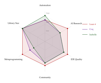
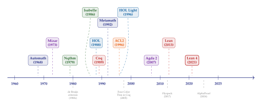
Why Lean 4 Is Winning
The claim that “Lean 4 is winning” requires immediate qualification: winning for AI-driven formalization, not necessarily winning for all use cases. Isabelle/HOL remains the system of choice for many industrial verification tasks. Coq remains dominant in programming language research. Agda remains the best environment for experimenting with advanced type theory. But for the specific goal of building AI systems that can do mathematics, Lean 4 has emerged as the clear leader. Several factors contribute.
A fast, modern compiler.
Lean 4's compiler generates efficient native code, making it feasible to run large-scale experiments (millions of tactic invocations) in reasonable time. Coq and Isabelle, by contrast, have slower execution environments that bottleneck training loops.
A general-purpose programming language.
Lean 4 is not just a proof assistant but a general-purpose functional programming language. This means that tools for interacting with Lean (parsing output, constructing tactic sequences, managing sessions) can be written in Lean itself, reducing the impedance mismatch between the prover and the AI infrastructure. Projects like LeanDojo exploit this by providing Python bindings that communicate with a Lean server [9].
Mathlib.
Mathlib is the largest coherent library of formalized mathematics in any system. As of 2024, it contains over 170,000 theorems, covers large portions of undergraduate and graduate mathematics, and is growing by hundreds of theorems per week. For AI, a large, well-organized, and actively maintained library is essential: it provides both the training data (theorem statements and proofs) and the infrastructure (lemmas and definitions) that generated proofs can build on.
Microsoft backing.
Lean 4 is developed by Leonardo de Moura's team at Microsoft Research. While Microsoft does not control the Lean community, its funding provides stability and resources (including a team of full-time developers) that volunteer-driven projects cannot match.
AI-friendliness.
Lean 4's design choices are unusually well-suited to AI:
The tactic mode provides a natural interface for generative models (generate one tactic at a time, observe the resulting proof state, generate the next tactic).
The metaprogramming framework allows custom interaction modes to be built without modifying the core system.
The Language Server Protocol (LSP) integration means that AI tools can communicate with Lean through a standard interface.
The Lean REPL allows programmatic evaluation of expressions and tactics.
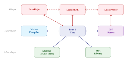
Cross-System Proof Transfer
A natural question is whether proofs can be transferred between different theorem provers. If the Four Color Theorem is proved in Coq and the Kepler Conjecture is proved in Isabelle, can we use both results in Lean 4 without re-proving them?
The short answer is: not easily. The obstacles are both foundational and practical.
Foundational obstacles.
Different provers use different logical foundations. Lean 4 and Coq both use the Calculus of Inductive Constructions, but with subtly different universe hierarchies and definitional equalities. Isabelle uses classical higher-order logic, which lacks dependent types but includes the axiom of choice and classical logic from the start. Mizar uses first-order set theory. These differences mean that a statement that is “obvious” in one system may require significant reformulation in another.
Practical obstacles.
Even when the foundations are compatible, the libraries are not. Lean's Mathlib defines real numbers as the completion of the rationals via Cauchy sequences. Coq's standard library uses Dedekind cuts. Isabelle's HOL-Analysis library uses a type class-based approach. Translating between these representations is possible in principle but tedious in practice.
Current approaches.
Several research projects are working on cross-system proof transfer:
Dedukti is a logical framework based on the -calculus modulo rewriting. It can encode the logics of Coq, HOL, and Lean as rewrite systems, enabling (in principle) translation between any two systems via Dedukti as an intermediate representation.
Statement alignment uses AI (typically embedding-based retrieval) to find corresponding theorems across different libraries. For example, a model might learn that Mathlib's
Nat.Primecorresponds to MathComp'sprimeand Isabelle'sprimepredicate.Proof replay translates tactic-level proofs by mapping tactics in one system to equivalent tactics in another. This is feasible for simple proofs but breaks down when tactics have no counterpart in the target system.
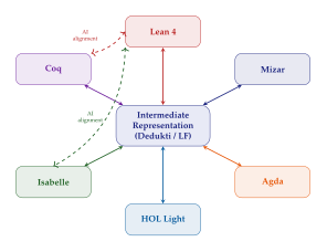
Will there be convergence?
It is tempting to predict that one system will eventually “win” and the others will fade. History suggests otherwise: Coq, Isabelle, and Mizar have coexisted for over three decades. Each system occupies a niche defined by its foundations, its community, and its accumulated library. What is more likely than convergence is interoperation: AI systems that can work with multiple provers, translating between them as needed, just as multilingual NLP systems can work with many languages [85].
Nevertheless, for the specific purpose of training generative models for mathematics, Lean 4 has achieved a critical mass of data (Mathlib), tooling (LeanDojo, REPL), and community momentum that makes it the default choice for new AI research projects as of 2024–2025. We expect this dominance to persist for at least the next several years.
Foundations and Trust
An important dimension of comparison is the size and complexity of the trusted computing base (TCB): the minimal set of code that must be correct for the system's proofs to be trustworthy.
For Lean 4, the TCB consists of the kernel type-checker (approximately 6,000 lines of C++ code in Lean's runtime) plus the axioms of the type theory. Everything else, including tactics, macros, and elaboration, is untrusted: a bug in a tactic can cause an incorrect proof attempt, but it cannot produce a proof that passes the kernel check.
For HOL Light, the TCB is remarkably small: about 400 lines of OCaml. This is possible because HOL's simple type theory has a much simpler kernel than CIC.
For Isabelle, the situation is intermediate: the kernel is larger than HOL Light's but is augmented by the Isabelle/Isar framework, and results proved via Sledgehammer are reconstructed internally.
For Metamath, the TCB is minimal by design: a Metamath proof checker can be implemented in under 300 lines of code in many languages, and dozens of independent implementations exist.
Remark 14.
The size of the TCB is not the only factor in trustworthiness. A small TCB that has been reviewed by many eyes (like HOL Light's) may be more trustworthy than a medium TCB (like Lean 4's) that fewer people have audited. On the other hand, a system with a larger TCB can offer more sophisticated features (dependent types, universe polymorphism, definitional proof irrelevance) that make formalization more practical. As with many engineering trade-offs, there is no universal optimum.
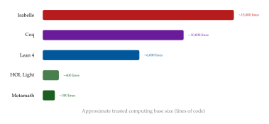
The Role of Libraries
The utility of a theorem prover depends critically on its formal library. A beautiful type theory with an empty library is useless for practical formalization. Table 2 compares the major formal libraries.
| Library | System | Theorems | Lines | Notable coverage |
| Mathlib | Lean 4 | 170,000+ | 1,000,000+ | Algebra, analysis, topology, number theory, measure theory |
| MathComp | Coq | 15,000+ | 200,000+ | Finite groups, representation theory, algebraic structures |
| AFP | Isabelle | 80,000+ | 3,000,000+ | Analysis, algebra, CS theory, probability |
| MML | Mizar | 60,000+ | 2,000,000+ | Set theory, topology, functional analysis |
| set.mm | Metamath | 40,000+ | 300,000+ | ZFC, algebra, analysis, number theory |
| Agda stdlib | Agda | 5,000+ | 100,000+ | Basic algebra, category theory, type theory |
The raw numbers are misleading without context. Isabelle's AFP has the most lines of code, but many entries are independent and not organized into a coherent library. Mathlib is monolithic and internally consistent: every definition builds on every other, and the entire library is checked as a single unit. This coherence makes Mathlib uniquely valuable for AI: a model trained on Mathlib can expect that any lemma it invokes will be compatible with any other lemma in the library.
Implications for AI Research
The diversity of theorem provers has important implications for AI research in formalization:
Training data.
Each formal library represents a corpus of human-written proofs in a specific formal language. A model trained exclusively on Mathlib cannot generate Coq proofs (and vice versa), but the underlying mathematical reasoning is the same. This suggests that multilingual models, trained on multiple formal libraries simultaneously, could transfer reasoning skills across systems, much as multilingual language models transfer linguistic knowledge across languages [86].
Evaluation.
Evaluating AI theorem provers is complicated by the diversity of systems. A model that solves 50% of Lean 4 benchmarks and a model that solves 50% of Isabelle benchmarks are not necessarily comparable, because the benchmarks may differ in difficulty, domain, and proof style. Standardized, cross-system benchmarks would be valuable but are hard to construct because of the foundational and library differences discussed above.
Tool integration.
AI tools must interface with the theorem prover's interactive mode. Each prover has its own interface: Lean 4 has the LSP and REPL, Coq has SerAPI and coq-lsp, Isabelle has PIDE (Prover IDE), and HOL Light has an OCaml toplevel. Building infrastructure for AI interaction is a significant engineering effort, and the existence of tools like LeanDojo [9] for Lean 4 and CoqGym [87] for Coq has directly driven the choice of system in many AI papers.
Key Idea.
The choice of theorem prover for AI research is driven not only by the prover's theoretical merits but also by the availability of (1) a large, coherent formal library for training data, (2) programmatic interfaces for AI interaction, and (3) an active community that produces new formalized mathematics at scale. As of 2024–2025, Lean 4 leads on all three dimensions, but this could change if other systems develop comparable AI-facing infrastructure.
Exercises for Section 7
Exercise 30.
The following is a Coq proof of the commutativity of addition on natural numbers:
Theorem add_comm : forall n m : nat, n + m = m + n.
Proof.
intros n m. induction n as [|n' IHn'].
- simpl. rewrite Nat.add_0_r. reflexivity.
- simpl. rewrite IHn'. rewrite Nat.add_succ_r. reflexivity.
Qed.
intros, induction,
simpl, rewrite, reflexivity). Which
Lean 4 tactic could close the goal in a single step?Exercise 31.
Explain the Sledgehammer architecture in Isabelle. In particular:
What external provers does Sledgehammer typically call?
Why is the proof found by an external prover not directly trusted?
What is “proof reconstruction,” and why is it sometimes slower than the original external proof search?
Could a similar architecture be implemented for Lean 4? What would be the main challenges?
Exercise 32.
Cubical Agda provides a computational interpretation of the univalence axiom. Explain what univalence means informally, and give an example of a mathematical statement that becomes easy to prove with univalence but is cumbersome without it. Why might univalence be relevant to AI systems that reason about mathematical structures “up to isomorphism”?
Exercise 33.
Consider the statement “every finite group of order (a prime) is cyclic.” This is proved in Mathlib (Lean 4), MathComp (Coq), and the AFP (Isabelle).
Find (or state) the theorem in each system.
Identify the key differences in how “finite group,” “order,” and “cyclic” are defined across the three systems.
Discuss the feasibility of automatically translating the Lean proof to Coq or Isabelle. What would an AI system need to handle?
Exercise 34.
The trusted computing base (TCB) of a theorem prover determines the degree of trust we can place in its proofs.
Explain why a bug in the
simptactic implementation cannot lead to an incorrect theorem being accepted in Lean 4.Describe a scenario in which a bug in Lean 4's kernel type-checker could lead to an incorrect theorem being accepted.
Metamath's extremely small TCB has led to dozens of independent proof checkers. What is the probability argument for why this provides strong assurance?
Exercise 35.
Design (on paper) a “multilingual” training dataset for an AI theorem prover that includes proofs from Lean 4, Coq, and Isabelle. Address the following:
How would you align theorem statements across systems?
Would you train a single model or separate models per system?
How would you handle the different proof styles (tactic-based in Lean/Coq, Isar-style in Isabelle)?
What evaluation metrics would you use to assess cross-system generalization?
Exercise 36.
Predict the state of the theorem prover ecosystem in 2030. Consider the following questions:
Will Lean 4 still be the dominant system for AI research? What could change this?
Will there be a new system that surpasses all current ones? What features would it need?
Will cross-system proof transfer become practical?
Will AI reduce the importance of the choice of prover by making all systems equally easy to use?
Write a brief (1–2 paragraph) argument for the scenario you consider most likely.
Classical Automated Theorem Proving
The dream of reducing reasoning to computation is older than computers themselves. Long before silicon circuits could evaluate a single Boolean formula, philosophers and mathematicians imagined machines that would settle disputes, verify arguments, and extend the frontiers of knowledge through purely mechanical manipulation of symbols. This section traces that dream from its philosophical origins through the sophisticated automated theorem provers (ATPs) of the early twenty-first century, arriving at a clear picture of what classical methods can and cannot do, and why the arrival of generative models represents a genuine paradigm shift.
Understanding classical ATP is essential for appreciating the contributions of generative models to mathematics. Many of the most successful modern systems combine neural generation with classical verification: the generative model proposes proof steps, and a classical prover checks them. Without understanding the checker, we cannot understand the system.
Key Idea.
Classical automated theorem proving treats proof search as a combinatorial problem: given a set of axioms and a conjecture, systematically explore the space of possible derivations until a proof (or refutation) is found. The power of this approach lies in its soundness and completeness guarantees; its limitation lies in the combinatorial explosion that renders most interesting mathematical problems intractable without human-like insight.
The Dream of Mechanical Reasoning
In 1666, Gottfried Wilhelm Leibniz, then a twenty-year-old student at the University of Altdorf, published his Dissertatio de Arte Combinatoria, in which he outlined a breathtaking vision: a characteristica universalis, a universal formal language capable of expressing all human thought, and a calculus ratiocinator, a mechanical procedure for deciding the truth or falsity of any statement expressed in that language [88]. When two philosophers disagreed, Leibniz wrote, they would need only sit down together, take up their pens, and say: “Calculemus” (let us calculate).
Leibniz's vision was far ahead of his time, and he never came close to realising it. But the dream persisted. In the nineteenth century, George Boole developed his algebra of logic [89], showing that at least some forms of reasoning could be reduced to algebraic manipulation. Augustus De Morgan formalised the laws that bear his name. Gottlob Frege constructed the first complete system of predicate logic [90].
The dream reached its most precise formulation in 1928, when David Hilbert and Wilhelm Ackermann posed the Entscheidungsproblem (decision problem): is there an algorithm that takes as input a statement in first-order logic and determines, in finitely many steps, whether that statement is universally valid? [91] If such an algorithm existed, it would be Leibniz's calculus ratiocinator made real.
The answer, as we now know, is no. In 1936, Alonzo Church and Alan Turing independently proved that the Entscheidungsproblem is undecidable: no algorithm can decide the validity of all first-order sentences [92][93]. This was a fundamental negative result. But it was not the end of the story. Undecidability means that no single algorithm can solve all instances. It does not mean that clever algorithms cannot solve many instances, and indeed that is precisely what the subsequent eighty years of research have shown.
Remark 15.
The undecidability of first-order validity does not prevent automated provers from being enormously useful. First-order logic is semi-decidable: if a sentence is valid, there exists a proof, and a systematic search will eventually find it. The problem is that if a sentence is not valid, the search may run forever. In practice, provers use time limits and heuristics to handle this.
Resolution-Based Proving
The modern era of automated theorem proving begins with J. Alan Robinson's 1965 paper introducing the resolution principle [22]. Resolution is a single inference rule that, when combined with a systematic search strategy, is refutation complete for first-order logic: if a set of clauses is unsatisfiable, resolution will derive the empty clause (a contradiction) in finitely many steps.
Before describing resolution, we must establish the logical framework in which it operates.
Propositional Logic: SAT Solving
The simplest setting is propositional logic. A propositional formula is built from Boolean variables using the connectives (not), (and), (or), (implies), and (if and only if). The satisfiability problem (SAT) asks: given a propositional formula , is there an assignment of truth values to the variables that makes true?
Definition 11 (Conjunctive Normal Form).
A propositional formula is in conjunctive normal form (CNF) if it is a conjunction of clauses, where each clause is a disjunction of literals (a variable or its negation): (CNF) Any propositional formula can be converted to an equisatisfiable CNF formula in polynomial time using the Tseitin transformation [21].
The propositional resolution rule is simple: from two clauses and , derive the resolvent . The variable is resolved upon. If both and are empty, the resolvent is the empty clause , indicating unsatisfiability.
The DPLL algorithm.
The Davis–Putnam–Logemann–Loveland (DPLL) algorithm, introduced in 1962 [94], is the foundation of all modern SAT solvers. DPLL combines three key ideas:
Unit propagation. If a clause contains only one unassigned literal, that literal must be true. Assign it and simplify the formula.
Pure literal elimination. If a variable appears only positively (or only negatively) in all remaining clauses, assign it to make all its occurrences true.
Branching. Choose an unassigned variable, assign it true, and recurse. If a contradiction is found, backtrack and try false.
DPLL performs a depth-first search over the space of partial assignments, using unit propagation and pure literal elimination to prune the search tree. In the worst case, the search tree has leaves (one for each complete assignment), but in practice the pruning is remarkably effective.
Conflict-driven clause learning.
The major breakthrough that transformed SAT solving from a theoretical curiosity into a practical powerhouse was conflict-driven clause learning (CDCL), developed by Marques-Silva and Sakallah [95] and independently by Bayardo and Schrag [96].
CDCL extends DPLL with two crucial mechanisms:
Clause learning. When a conflict is detected (unit propagation derives both and ), the solver analyses the conflict to identify a conflict clause: a new clause that captures the reason for the conflict. This clause is added to the formula, preventing the solver from making the same mistake again.
Non-chronological backtracking. Instead of backtracking to the most recent decision (as in DPLL), CDCL jumps back to the earliest decision level that is relevant to the conflict. This can skip many levels of the search tree.
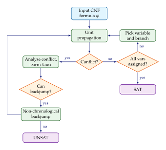
Modern SAT solvers such as MiniSat [97], CaDiCaL [98], and Kissat implement CDCL with numerous additional techniques: variable state independent decaying sum (VSIDS) heuristics for variable selection, restarts to escape unproductive regions of the search space, and inprocessing (simplifying the formula during search).
The practical impact of CDCL is staggering. Industrial SAT instances with millions of variables and clauses are now solved routinely. The annual SAT Competition drives continuous improvements, and SAT solvers underpin everything from hardware verification to planning to cryptanalysis.
First-Order Logic: Unification and Resolution
Propositional logic is limited: it cannot express quantified statements like “for all natural numbers , if is even then is even.” First-order logic (FOL) adds variables, quantifiers (, ), functions, and predicates, enabling the expression of most mathematical statements.
Resolution in first-order logic requires an additional mechanism: unification. Given two atoms and , a unifier is a substitution such that . The most general unifier (MGU) is the unifier that makes the fewest commitments.
Definition 12 (Most General Unifier).
A substitution is a most general unifier of two terms and if:
(i.e., is a unifier), and
for every other unifier , there exists a substitution such that (i.e., is more general than ).
The MGU can be computed in quasi-linear time by Robinson's unification algorithm [22].
First-order resolution then proceeds as follows. Given clauses and , where and can be unified with MGU , derive the resolvent . Combined with Skolemization (replacing existential quantifiers with Skolem functions) and clausification (converting to clause normal form), resolution is refutation complete for first-order logic.
Paramodulation.
Equality is pervasive in mathematics. The axiom means that can be replaced by in any context. Handling equality within resolution requires a special inference rule called paramodulation: from a clause containing and another clause containing a subterm matching , derive a new clause with that subterm replaced by .
Formally, if and where unifies with via MGU , then paramodulation derives . Modern provers use ordered paramodulation and superposition calculus to restrict the application of this rule to cases where it is likely to be productive [99].
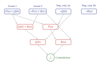
Major first-order provers.
Three systems dominate the landscape of first-order automated theorem proving:
Vampire, developed by Voronkov and Kovács [23], has won the most divisions of the annual CASC (CADE ATP System Competition) of any prover. Vampire implements superposition with a sophisticated set of simplification and redundancy elimination techniques.
E prover, developed by Schulz [24], is an open-source superposition prover known for its flexibility and extensibility. E's clause selection heuristics can be configured through a rich set of parameters, making it a popular platform for machine learning integration.
SPASS, developed by Weidenbach and colleagues [25], combines superposition with splitting and other inference rules. SPASS has been particularly influential in the development of the superposition calculus.
These provers routinely solve problems in first-order logic with equality that would be far beyond human capacity if approached purely mechanically. They are the workhorses of formal verification, and as we shall see in later sections, they serve as the verification backends for many neural theorem proving systems.
Satisfiability Modulo Theories
Resolution-based provers operate in “pure” first-order logic. But many practical verification and reasoning tasks involve domain-specific operations: arithmetic, arrays, bit vectors, strings. Encoding these operations in raw first-order logic is possible but extremely inefficient. Satisfiability Modulo Theories (SMT) solvers address this by combining a SAT solver with specialised theory solvers that understand the semantics of specific domains [26].
Definition 13 (SMT Problem).
An SMT problem is a satisfiability problem in first-order logic where certain function and predicate symbols are given fixed interpretations by a background theory . Formally, given a formula and a theory , the SMT problem asks: is satisfiable in a model of ?
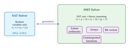
Major SMT Solvers
The three most widely used SMT solvers are:
Z3, developed at Microsoft Research by de Moura and Bjrner [26], is arguably the most influential SMT solver. Z3 supports a vast array of theories (linear and nonlinear arithmetic over integers and reals, bit vectors, arrays, strings, floating-point arithmetic, algebraic datatypes, sequences, and regular expressions) and has been integrated into hundreds of tools for program analysis, verification, synthesis, and testing.
CVC5, the latest in the CVC family developed at Stanford and the University of Iowa [27], is Z3's closest competitor. CVC5 excels at quantified formulas and has strong support for strings and regular expressions. It also supports syntax-guided synthesis (SyGuS), where the solver constructs programs that satisfy a given specification.
Yices, developed at SRI International [28], is known for its efficiency on linear arithmetic and bit-vector problems. Yices was the first solver to win the SMT Competition in all main-track divisions simultaneously.
Theories and Their Applications
The power of SMT comes from the breadth of supported theories. Each theory provides a decision procedure for formulas involving its function symbols, and the DPLL() framework combines these procedures with a Boolean backbone [100].
Linear arithmetic (, ): supports , , , , , and multiplication by constants, over integers (LIA) or reals (LRA). The Simplex algorithm underlies most LRA solvers; LIA adds branch-and-bound or Omega test.
Arrays () : supports
select(read) andstore(write) operations. The theory is axiomatised by the read-over-write axiom: and .Bit vectors () : supports fixed-width binary arithmetic, bitwise operations, shifting, and extraction. Essential for hardware and low-level software verification.
Uninterpreted functions () : the simplest theory, asserting only that equal arguments yield equal results (the congruence axiom). Combined with other theories via the Nelson–Oppen or Shostak combination methods.
SMT solvers have applications far beyond pure mathematics. They are central to:
Software verification: checking that programs satisfy their specifications (e.g., Dafny [29], Frama-C).
Bounded model checking: verifying hardware circuits up to a fixed depth.
Planning: encoding planning problems as SMT formulas.
Test generation: generating test inputs that cover specific program paths (e.g., KLEE [30]).
Symbolic execution: exploring program paths with symbolic inputs.
Example 28.
Software verification with SMT. Consider a simple function that computes the absolute value of an integer:
int abs(int x) {
if (x >= 0) return x;
else return -x;
}
Example 29.
Constraint-based scheduling. SMT solvers can encode complex scheduling problems. Suppose we have tasks with durations , start times , and resource requirements. The constraint that tasks and cannot overlap on the same resource is: Combined with deadline constraints () and precedence constraints ( for dependent tasks), the full scheduling problem becomes an SMT formula over linear integer arithmetic. Modern SMT solvers can handle instances with thousands of tasks and constraints.
The interaction between the SAT core and the theory solvers is governed by the DPLL() framework [100]. The SAT solver proposes a Boolean assignment to the “theory atoms” (the atomic formulas involving theory symbols). The theory solver then checks whether this assignment is consistent with the theory. If not, the theory solver produces a theory conflict clause that explains why the assignment is inconsistent, and the SAT solver uses this clause to guide its search (exactly as it would use a learned clause in CDCL). This lazy approach avoids the need to eagerly enumerate all theory consequences, and it has proven remarkably effective in practice.
Exercise 37.
SMT theory combination. Consider the formula: This formula involves both uninterpreted functions and linear integer arithmetic.
Identify which atoms belong to which theory.
Use the Nelson–Oppen combination method to determine whether the formula is satisfiable.
What equalities must be shared between the theory solvers?
Interactive Theorem Proving with Automation
Automated theorem provers and SMT solvers excel at small, well-defined logical problems. But most real mathematical theorems are far too complex for any ATP to prove from scratch. The proof of the Feit–Thompson theorem (that every finite group of odd order is solvable) spans thousands of pages; the formalisation in Coq required over 170,000 lines of code [16]. For such theorems, human mathematicians (or human formalisers) must provide the overall proof strategy, breaking the proof into lemmas small enough for automation to handle.
This is the domain of interactive theorem provers (ITPs), also called proof assistants: systems in which a human user guides the proof while the machine checks each step and, increasingly, automates the tedious parts. The leading ITPs include:
Isabelle/HOL: based on higher-order logic, with a rich library (the Archive of Formal Proofs) and powerful automation.
Coq: based on the Calculus of Inductive Constructions (CIC), with dependent types and a tactic language (Ltac, Ltac2).
Lean: a newer system with a modern type theory, a growing mathematical library (Mathlib), and strong community engagement.
HOL Light: a minimalist higher-order logic prover, used for the Flyspeck project (formal verification of the Kepler conjecture) [7].
Sledgehammer: bridging ITPs and ATPs.
The most celebrated bridge between interactive and automated theorem proving is Isabelle's Sledgehammer [65]. Sledgehammer automates the most tedious step of interactive proving: finding which previously proved lemmas are needed and showing that they imply the current goal.
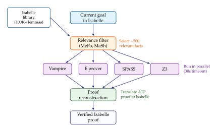
metis or smt.Sledgehammer operates in three phases:
Relevance filtering. The Isabelle library contains hundreds of thousands of lemmas. Sending all of them to an ATP would overwhelm it. Sledgehammer uses two complementary filters: itemize
MePo (Meng–Paulson filter): a symbol-based heuristic that selects lemmas sharing function and predicate symbols with the current goal.
MaSh (Machine Learning for Sledgehammer): a machine learning system that learns from past proofs which lemmas are likely to be useful for goals with similar features [31]. itemize Typically, about 500 relevant facts are selected.
ATP invocation. The selected facts and the negated goal are translated into first-order logic (using various encoding strategies for higher-order features) and sent to multiple ATPs (Vampire, E, SPASS) and SMT solvers (Z3, CVC5) in parallel, each with a timeout (typically 30 seconds).
Proof reconstruction. If an ATP finds a proof, its output must be translated back into a verified Isabelle proof. Sledgehammer uses
metis(a built-in resolution prover) or thesmtmethod to reconstruct the proof within Isabelle's trusted kernel, ensuring that the ATP's result is independently verified.
Sledgehammer's success rate is impressive. On typical Isabelle proof obligations, Sledgehammer can close 40–50% of goals automatically, dramatically reducing the human effort required for formalisation [65].
CoqHammer.
CoqHammer [101] brings similar functionality to the Coq proof assistant. The architecture mirrors Sledgehammer's: relevance filtering selects lemmas from Coq's library, translation converts the goal and lemmas to first-order logic, external ATPs search for proofs, and reconstruction rebuilds the proof within Coq's type-theoretic kernel.
The translation from Coq to first-order logic is more challenging than from Isabelle, because Coq's type theory (the Calculus of Inductive Constructions) is more expressive than Isabelle's higher-order logic. Dependent types, universe polymorphism, and inductive families must all be encoded, and the encoding necessarily loses information. Despite these challenges, CoqHammer achieves success rates of 30–40% on standard Coq proof obligations.
Exercise 38.
Resolution proof construction. Given the clauses:
Construct a resolution proof that derives the empty clause . At each step, identify the resolved literals and the most general unifier used.
Exercise 39.
CDCL conflict analysis. Consider the CNF formula with clauses: Trace the execution of the CDCL algorithm. At the point of conflict, identify the conflict clause that would be learned. To which decision level does the solver backjump?
Exercise 40.
SMT encoding. Encode the following problem as an SMT formula over the theory of linear integer arithmetic: “Find integers , , such that , , , , and . Maximise .” Explain how an SMT solver would determine the optimal value of .
Limitations of Classical ATP
Classical automated theorem provers are among the great achievements of computer science. They are sound, they are (semi-)complete, and they can solve problems that would take humans years. Yet they have fundamental limitations that motivate the search for new approaches.
No mathematical understanding.
A resolution prover does not “understand” mathematics. It manipulates symbols according to inference rules, without any concept of what those symbols mean. It cannot look at a formula and think, “This looks like it should follow from the intermediate value theorem.” It cannot recognise that a proof is “elegant” or “natural.” It cannot draw an analogy between two different areas of mathematics.
Example 30.
Consider the classical proof that is irrational. A human mathematician sees the structure immediately: assume in lowest terms, square both sides, derive a contradiction about divisibility. The proof is four lines of human reasoning. A resolution prover, presented with the same problem formalised in first-order logic, would need to search through a vast space of possible inferences, most of which are irrelevant. It would eventually find a proof, but the proof would be a sprawling resolution tree with hundreds of steps, bearing no resemblance to the human proof.
Combinatorial explosion.
The search space of resolution grows exponentially with the number of clauses and the depth of terms. For problems in domains like group theory, ring theory, or combinatorics, the number of possible inferences at each step is enormous, and most branches of the search tree lead nowhere. Heuristics help, but they cannot eliminate the fundamental exponential nature of the search.
No concept discovery.
Perhaps the most fundamental limitation is that classical ATPs cannot discover new concepts. A prover can only work with the concepts that are already present in the axioms and the goal. It cannot invent a new definition, introduce an auxiliary construction, or reformulate a problem in a more tractable form. Yet concept discovery is at the heart of mathematical creativity.
Key Idea.
The limitations of classical ATP are not merely practical (insufficient speed or memory) but fundamental: they arise from the paradigm of treating proof search as combinatorial search over inference rules. What is missing is mathematical intuition: the ability to recognise patterns, draw analogies, and propose creative proof strategies. This is precisely what generative models aim to provide.
The knowledge bottleneck.
An ATP has access only to the axioms and lemmas it is given. In contrast, a human mathematician draws on a vast background of mathematical knowledge: techniques from analysis applied to number theory, topological arguments in algebra, probabilistic methods in combinatorics. This cross-pollination of ideas is central to mathematical progress, and classical ATPs have no mechanism for it.
Inability to handle informal reasoning.
The vast majority of mathematical communication occurs in natural language, supplemented by formal notation. Textbooks, research papers, lectures, and mathematical conversations all use a blend of rigour and informality that is inaccessible to classical ATPs. When a mathematician says “by a standard compactness argument,” a human reader understands what this means and can fill in the details. An ATP has no mechanism for interpreting such informal guidance.
Example 31.
The four-colour theorem. The computer-assisted proof of the four-colour theorem [32] illustrates both the power and limitations of automated reasoning. The proof reduces the problem to checking a finite (but large) number of cases, each of which can be verified by a computer. The overall proof strategy, however, was devised by humans (Appel and Haken). The computer verified the cases; it did not discover the proof structure. This division of labour (human strategy, machine verification) anticipates the modern paradigm of neural generation with formal verification.
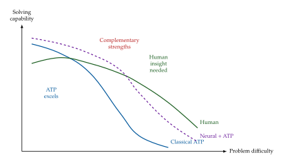
Exercise 41.
Analysing the search space. Consider a set of clauses in propositional logic, each containing exactly literals. Derive an upper bound on the number of possible resolvents that can be generated in one step of resolution. How does this bound grow as increases? Use your bound to estimate the size of the search space for and .
Exercise 42.
The limits of relevance filtering. Suppose an Isabelle library contains lemmas, and a relevance filter selects a subset of lemmas for a given goal. Assume the true set of needed lemmas has size .
What is the probability that all needed lemmas are in the selected subset, if the filter selects uniformly at random? (You may express your answer as a binomial coefficient.)
Explain why, despite this low probability, Sledgehammer achieves 40–50% success rates. What does this tell us about the distribution of “useful” lemmas?
Propose a way to combine relevance filtering with a generative model to improve the selection of useful lemmas.
The Mathematical Reasoning Landscape Before LLMs
By 2019, the landscape of machine-assisted mathematical reasoning was fragmented into distinct traditions, each powerful in its own domain but fundamentally limited. Computer algebra systems could compute but not prove. Automated theorem provers could prove but not understand. Interactive theorem provers required painstaking human guidance. And a nascent wave of neural approaches was beginning to show that machine learning could contribute to theorem proving, though the contributions were still modest.
This section surveys the state of affairs before the transformative impact of large language models, identifying both the achievements and the gaps that LLMs would later begin to fill. Understanding this landscape is essential for appreciating why the arrival of LLMs was such a significant event in the history of mathematical reasoning.
Computer Algebra Systems: Computation Without Proof
Computer algebra systems (CAS) are among the oldest and most successful tools for machine-assisted mathematics. Systems like Mathematica [102], Maple, SageMath [103], and SymPy [104] can perform symbolic differentiation and integration, solve equations, factor polynomials, compute limits, manipulate matrices, and carry out hundreds of other algebraic operations with speed and reliability that far exceeds human capability.
The key distinction, however, is between computation and proof. A CAS can compute that , but it does not produce a proof of this fact in any formal sense. It applies algorithms (Risch integration, Gröbner basis computation, etc.) that are known to be correct, but the correctness of the implementation is trusted, not verified.
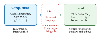
Remark 16.
Some efforts have been made to bridge the gap between CAS and
ITP. Projects like the Formal Abstracts
initiative and verified CAS algorithms
within proof assistants (e.g., verified polynomial
arithmetic in Isabelle) represent steps in this direction.
The norm_num
tactic in Lean can verify numerical computations within the
proof assistant. But these efforts cover only a fraction of
the computational capabilities of a full CAS.
Example 32.
The Risch algorithm and its limits. The Risch algorithm can determine whether an elementary function has an elementary antiderivative, and if so, compute it. For instance, it can prove that has no elementary closed form, and it can compute . But the Risch algorithm is a decision procedure, not a proof procedure: it tells us what the answer is, but it does not produce a machine-checkable proof that the answer is correct. Verifying the output of a CAS within a proof assistant requires a separate formalisation effort.
Example 33.
Gröbner bases in algebraic geometry. Buchberger's algorithm computes Gröbner bases for polynomial ideals, enabling the solution of systems of polynomial equations, ideal membership testing, and elimination of variables. A CAS can compute the Gröbner basis of the ideal in milliseconds, yielding and revealing that the solutions are . The computation is correct, but it exists in a different universe from a formal proof of the same fact in Lean or Isabelle.
The gulf between CAS and ITP is not merely a matter of software engineering. It reflects a deep conceptual distinction between knowing the answer and knowing why the answer is correct. A CAS computes answers using algorithms whose correctness has been proved by humans (in informal mathematics, published in journals). An ITP verifies every step against a small, trusted logical kernel. The CAS approach is efficient but relies on trust in complex software; the ITP approach is rigorous but painfully slow. Bridging this gap is one of the great promises of generative models.
The IMO Grand Challenge
In 2019, a group of researchers including Daniel Selsam (Microsoft Research), Kevin Buzzard (Imperial College London), and others issued the IMO Grand Challenge: to build an AI system capable of winning a gold medal at the International Mathematical Olympiad (IMO) [105].
The IMO is the most prestigious mathematical competition for pre-university students. Each year, roughly 600 contestants from over 100 countries solve six problems in two sessions of 4.5 hours each. The problems span algebra, combinatorics, geometry, and number theory, and they require deep mathematical insight, creative problem-solving, and rigorous proof construction. A gold medal typically requires solving four or more of the six problems.
The IMO Grand Challenge specifies two crucial requirements:
Formal proofs. The system must produce proofs that can be verified by a formal proof checker. Natural language arguments, no matter how convincing, do not count. This ensures that the system has genuinely “proved” its answers, not merely guessed them.
Time limit. The system must work within the same time constraints as human contestants: 4.5 hours per session of three problems.
As of 2019, no AI system came close to this goal. The best automated systems could handle only the simplest competition problems, and even then required significant human assistance in formalisation. The challenge crystallised the gap between the state of the art in AI and the level of mathematical reasoning that talented human teenagers achieve routinely.
Remark 17.
The IMO Grand Challenge is deliberately ambitious. Unlike benchmarks that measure performance on fixed test sets, the IMO presents new, never-before-seen problems each year. A system that can solve IMO problems must generalise to novel mathematical situations, not just memorise patterns from training data. This makes the IMO Grand Challenge one of the most meaningful benchmarks for mathematical AI.
Example 34.
An IMO problem (2019, Problem 1). Let be the set of integers. Determine all functions such that, for all integers and : This problem requires finding all solutions (not just verifying a given solution), a creative step that involves substituting special values, identifying patterns, and constructing a rigorous argument. As of 2019, no automated system could produce a formal proof of the answer ( for all , or for some constant ) within a reasonable time limit.
The IMO Grand Challenge served as a rallying point for the mathematical AI community. It made concrete what had previously been vague aspirations, and it set a standard against which progress could be measured. When DeepMind's AlphaProof system solved several IMO problems in 2024 (a development we discuss in later sections), the community could point to the IMO Grand Challenge as the benchmark that defined the goal.
Exercise 43.
Formalising an IMO problem. Take the functional equation from Example 34 and write a formal statement of the problem in the language of your preferred proof assistant (Lean, Coq, or Isabelle). Discuss the challenges you encounter in formalising the statement “determine all functions” as a formal proposition. In particular, how do you formalise the requirement that the answer is complete (no solutions are missing)?
Early Neural Approaches to Theorem Proving
The period from 2016 to 2020 saw a burst of activity in applying neural networks to theorem proving. These early efforts were modest in scope compared to what would come later, but they established many of the key ideas and architectures that subsequent work would build upon.
DeepMath: Predicting Premise Relevance
The first major application of deep learning to theorem proving was DeepMath, published by Alemi, Chollet, Irving, Szegedy, and Urban in 2016 [106].
DeepMath addressed a specific subproblem: premise selection. Given a conjecture to be proved, which of the thousands of available lemmas in the library are most likely to be useful? This is the same problem that Sledgehammer's MaSh filter addresses, but DeepMath tackled it with deep neural networks rather than hand-crafted features.
DeepMath trained convolutional neural networks (CNNs) and recurrent neural networks on the Mizar Mathematical Library, learning to predict whether a given premise was used in the proof of a given theorem. The results were encouraging: DeepMath's premise selection, when combined with the E prover, proved 7.36% of held-out Mizar theorems, compared to 4.98% for E with its default heuristics.
Key Idea.
DeepMath established a paradigm that would persist through much subsequent work: use neural networks not to replace classical provers but to guide them. The neural network provides the “intuition” (which premises look relevant?), while the classical prover provides the “rigour” (is the proof actually valid?).
The DeepMath approach highlighted a recurring theme: the bottleneck in automated theorem proving is often not the proving itself but the selection of relevant information. A library of 50,000 theorems contains a vast amount of useful knowledge, but presenting all of it to a prover is counterproductive. The prover drowns in irrelevant information and wastes its search budget exploring dead ends. Neural premise selection provides a principled way to filter this information, and subsequent work would refine this idea considerably.
Remark 18.
DeepMath's success on Mizar was particularly noteworthy because Mizar's logical foundations (a variant of Tarski–Grothendieck set theory) differ substantially from the type theories used by Coq and Lean. This demonstrated that neural approaches to theorem proving were not tied to any specific logical framework, a finding that would prove important as the field expanded to cover multiple proof assistants.
GamePad: Learning to Prove in Coq
In 2018, Huang, Dhariwal, Song, and Li [107] introduced GamePad, a system for learning to prove theorems in Coq.
GamePad framed theorem proving as a game: the “state” is the current proof goal (a formula to be proved, along with the available hypotheses), and the “actions” are the tactics that can be applied. A neural network, trained on a dataset of human-written Coq proofs, learned to predict which tactic to apply given the current goal.
The key technical contribution of GamePad was its representation of proof states. Coq proof goals are abstract syntax trees (ASTs) that can be very deep and complex. GamePad used tree-structured neural networks to encode these ASTs into fixed-dimensional vectors, enabling the neural network to reason about the structure of mathematical expressions.
GamePad demonstrated proof automation on the Feit–Thompson formalisation, one of the most complex formalisations in Coq. While the results were preliminary (GamePad could close only a small fraction of goals), the approach showed that neural networks could learn meaningful representations of formal mathematical objects.
HOList: Learning Theorem Proving in HOL Light
In 2019, Bansal, Loos, Rabe, Szegedy, and Wilcox [108] introduced HOList, a benchmark and learning environment for theorem proving in HOL Light.
HOList made several important contributions:
A large-scale benchmark. HOList extracted over 29,000 theorems from the core HOL Light library, along with their proofs, creating the largest benchmark for neural theorem proving at the time.
A reinforcement learning environment. HOList provided an API for interacting with HOL Light, enabling agents to attempt proofs, receive feedback (success or failure), and learn from experience.
Strong baselines. HOList demonstrated that a neural network trained to predict proof steps could, combined with beam search, prove 55.7% of held-out theorems, a substantial improvement over hand-coded heuristics.
GPT-f: Generative Language Models for Formal Proof
The most consequential pre-LLM neural theorem proving system was GPT-f, introduced by Polu and Sutskever in 2020 [2].
GPT-f represented a fundamental shift in how neural networks were applied to theorem proving. Where previous systems (DeepMath, GamePad, HOList) used neural networks to classify or select from a fixed set of actions, GPT-f used a generative language model to generate proof steps as text. The model was a Transformer decoder (based on the GPT architecture) trained on a dataset of formal proofs from the Metamath library.
Definition 14 (Generative Theorem Proving).
In generative theorem proving, a language model generates the next proof step (a tactic application, a term, or a complete proof fragment) conditioned on the current proof state, expressed as a string. The generated step is then checked by a formal verification kernel for validity.
The results were striking. GPT-f, combined with best-first search, proved 56.22% of held-out Metamath theorems and found 23 new proofs that were shorter than the existing human-written proofs. These new proofs were accepted into the Metamath library, marking the first time that an AI system contributed original proofs to a major mathematical library.
Remark 19.
The significance of GPT-f's contribution to the Metamath library should not be understated. Previous neural theorem proving systems demonstrated that neural networks could rediscover known proofs. GPT-f demonstrated that they could improve upon known proofs, finding shorter and more elegant alternatives. This moved the conversation from “can neural networks prove theorems?” to “can neural networks contribute to mathematics?” – a qualitatively different question with far-reaching implications.
The key architectural innovation of GPT-f was the treatment of proof steps as sequences of tokens rather than as structured objects. By encoding both the proof state and the proof step as strings, GPT-f could leverage the full power of the Transformer architecture, including its ability to capture long-range dependencies and its scalability to large datasets. This flattening of structure was initially controversial (one might expect that preserving the tree structure of mathematical expressions would be beneficial), but the results spoke for themselves.
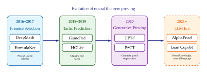
The Paradigm Shift: From Search to Generation
The progression from DeepMath to GPT-f reveals a fundamental paradigm shift in how neural networks interact with theorem provers.
DeepMath (2016): The neural network is a filter: it selects premises from a fixed library, then hands the problem to a classical prover. The prover still does all the reasoning.
GamePad/HOList (2018–2019): The neural network is a policy: it selects tactics from a fixed set of options. The prover still executes the tactics, but the neural network guides the search.
GPT-f (2020): The neural network is a generator: it produces proof steps as text, drawing on its training to construct novel tactic invocations with appropriate arguments. The prover becomes a verifier, checking the generated steps rather than producing them.
This shift from search-based to generation-based proving has profound implications. In the search paradigm, the prover explores a combinatorial space defined by the inference rules. In the generation paradigm, the model draws on learned patterns to propose proof steps directly, bypassing much of the combinatorial search. The trade-off is that the generated steps may be incorrect (the model “hallucinates”), but the formal verification kernel catches all errors.
Proposition 2 (Complementarity of Generation and Verification).
Let be a generative model that proposes proof steps with probability of producing a valid step, and let be a sound verifier. In a proof of steps, the expected number of model queries before the proof is completed is: (GEN Verify) where is the probability of generating a correct step and . Crucially, the correctness of the final proof depends only on the soundness of , not on the reliability of .
Proof.
Each step requires a geometric number of attempts with parameter , so the expected number of attempts for step is . By linearity of expectation, the total expected queries is the sum . The upper bound follows from bounding each term by . Soundness of the complete proof follows from the soundness of : every accepted step is valid, regardless of how it was generated.
What Was Missing Before LLMs
Despite the progress of 2016–2020, several critical capabilities were missing from the pre-LLM landscape:
Broad mathematical knowledge.
Pre-LLM neural theorem provers were trained on specific formal libraries (Mizar, HOL Light, Metamath). They learned the patterns within those libraries, but they had no access to the vast informal mathematical knowledge contained in textbooks, research papers, lecture notes, and online forums. A system trained on Metamath's library of 38,000 theorems has a very different knowledge base from a mathematician who has read hundreds of papers across multiple subfields.
Natural language understanding.
Mathematical reasoning is conducted largely in natural language, supplemented by formal notation. A mathematician reading a proof switches fluidly between English (or French, or any other natural language) and symbols. Pre-LLM systems operated entirely in the formal language of their proof assistant, with no ability to understand or produce natural language mathematics.
Proof sketching.
Human mathematicians typically work by first constructing a proof sketch: a high-level outline that captures the key ideas without filling in all the details. They then refine the sketch, adding rigour where needed. Pre-LLM systems had no mechanism for this kind of hierarchical planning. They generated proofs one step at a time, with no ability to “step back” and consider the overall proof strategy.
Autoformalization.
The vast majority of mathematics is written in natural language, not in formal logic. Autoformalization, the task of automatically translating natural language mathematics into formal specifications, was essentially unsolved before LLMs. This created a bottleneck: even if a prover could find a proof once the problem was formalised, the formalisation step itself required expert human effort.
Cross-domain transfer.
Some of the most beautiful proofs in mathematics draw on unexpected connections between different areas. Erdos's probabilistic method uses probability theory to prove combinatorial results. The proof of Fermat's Last Theorem connects number theory, algebraic geometry, and the theory of modular forms. Pre-LLM theorem provers, trained on a single formal library, had no mechanism for this kind of cross-domain transfer. They could not “borrow” a technique from analysis to prove a result in combinatorics, because they had no understanding of the analogies that make such borrowing possible.
Informal-to-formal translation.
The gap between informal and formal mathematics is vast. Consider the statement: “A continuous function on a closed interval attains its maximum.” A human mathematician instantly understands this as the extreme value theorem. Translating it into a formal statement requires specifying the types (real-valued function on ), the topology (the standard topology on ), the definition of continuity (- or via open sets), and the definition of “attains” (). Before LLMs, this translation was a manual process requiring expertise in both mathematics and the target proof assistant.
Key Idea.
The pre-LLM era of neural theorem proving was characterised by a mismatch between the narrow, formal nature of the proof environments and the broad, informal nature of mathematical reasoning. LLMs, trained on the entire internet (including textbooks, papers, and forums), would begin to bridge this gap by bringing broad mathematical knowledge to bear on formal proof search.
The Role of Search in Theorem Proving
Whether the proof steps are generated by classical inference rules or by neural networks, the fundamental computational structure of theorem proving is search. The proof state defines a tree (or, more generally, a directed acyclic graph) in which each node is a proof state and each edge is a proof step. The root is the initial goal, and the leaves are either closed goals (success) or dead ends (failure). The prover must find a path from the root to a state in which all goals are closed.
Theorem 8 (Proof Search as Graph Exploration).
Let be the proof search graph, where is the set of proof states and is the set of valid proof steps. Let be the initial state (the conjecture), and let be the set of terminal states (all goals closed). Finding a proof is equivalent to finding a path from to some in .
The graph has the following properties:
Branching factor. At each non-terminal state , the number of applicable proof steps (the out-degree) may range from zero to infinity (in the first-order case, where terms can be arbitrarily complex).
Depth. The shortest proof may have depth , but the search may explore states at much greater depth before finding it.
Redundancy. Multiple paths may lead to the same state, and the graph may contain cycles.
Without a good search strategy, the number of states explored grows exponentially in the depth: , where is the effective branching factor.
Proof.
The correspondence between proof search and graph exploration is direct. Each proof state is a tuple of unsolved goals and the current proof context. A proof step transforms into a new state by applying a tactic (in an ITP) or an inference rule (in an ATP). A proof is complete when the resulting state has no unsolved goals, i.e., belongs to . The exponential bound on the number of explored states follows from the standard analysis of tree search: a tree of depth with branching factor has nodes.
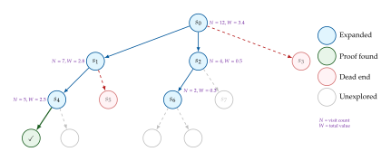
Three search algorithms have proven particularly effective for neural theorem proving:
Best-first search.
In best-first search, the prover maintains a priority queue of unexplored proof states, ranked by a value function that estimates the probability that a proof can be found from state . At each step, the highest-valued state is expanded. When the value function is provided by a neural network, this approach combines the neural network's “intuition” about which states are promising with a systematic exploration strategy.
(BEST First) where is the set of unexpanded states and is a learned value function.
Monte Carlo Tree Search.
MCTS, made famous by its role in AlphaGo, adapts naturally to theorem proving. MCTS balances exploration (trying new proof steps) with exploitation (pursuing promising directions) using the UCB (Upper Confidence Bound) formula: (UCB) where is the cumulative value of taking action from state , is the number of times action has been tried from state , , and is an exploration constant.
MCTS for theorem proving operates in four phases:
Selection. Starting from the root, use the UCB formula to select actions until reaching an unexpanded node.
Expansion. Apply the neural policy to generate candidate proof steps at the unexpanded node.
Simulation/Evaluation. Use the value network to estimate the probability of success from the new state.
Backpropagation. Update the visit counts and value estimates along the path from the new node back to the root.
Expert iteration.
Expert iteration, introduced by Anthony, Tian, and Barber [109], is a reinforcement learning framework that alternates between two phases:
Search (expert). Use MCTS (or another search algorithm) with the current policy to find proofs. The search acts as an “expert” that is stronger than the raw policy because it explores multiple possibilities.
Learning (apprentice). Train the policy network on the proof trajectories found by the search, so that the policy learns to imitate the expert.
The key insight is that the search (expert) is always better than the raw policy (apprentice), because the search explores multiple branches. By training the policy to imitate the search, the policy improves. Then the improved policy makes the search stronger (because the search uses the policy as a prior), which generates even better training data, and so on. This creates a virtuous cycle of self-improvement.
(Expert ITER) where is the dataset of (state, action) pairs collected by MCTS in iteration , is the neural policy, and is the improved policy from MCTS using as the prior.
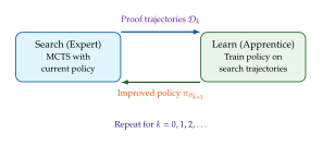
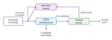
Pre-LLM Neural Theorem Proving: A Comparison
To consolidate our understanding of the pre-LLM neural theorem proving landscape, we present a systematic comparison of the major systems.
| System | Year | Environment | Architecture | Role | Key Result |
| DeepMath | 2016 | Mizar | CNN, RNN | Premise selection | 7.36% prove rate with E prover |
| FormulaNet | 2017 | HOL Light | Graph NN | Premise selection | Improved premise ranking |
| GamePad | 2018 | Coq | TreeRNN | Tactic prediction | Proof automation on Feit–Thompson |
| HOList | 2019 | HOL Light | GNN, WaveNet | Policy + value | 55.7% prove rate |
| GPT-f | 2020 | Metamath | Transformer | Proof generation | 56.22% prove rate, 23 new proofs |
| PACT | 2020 | Lean | Transformer | Proof generation | Improved with co-training |
Several trends emerge from this comparison:
Increasing neural autonomy. The role of the neural network evolved from a passive filter (DeepMath) to an active generator (GPT-f). Each successive system gave the neural network more responsibility for the creative work of proof construction.
Architectural convergence. Early systems used specialised architectures (CNNs for token sequences, tree-structured RNNs for ASTs, graph neural networks for formula structure). By 2020, the Transformer had become dominant, thanks to its ability to handle variable-length inputs and its scalability.
Growing scale. Training datasets grew from thousands of examples (DeepMath) to tens of thousands (HOList, GPT-f). Model sizes grew correspondingly, though they remained small by the standards of the LLM era that was about to begin.
Persistent verification. Across all systems, the formal verification kernel remained the final arbiter of correctness. This principle – that the neural network proposes and the kernel verifies – would persist into the LLM era and remains a cornerstone of neural theorem proving.
Exercise 44.
Branching factor analysis. Consider a theorem proving system where the neural policy assigns probability to each of possible tactics at each proof state, sorted so that . Define the effective branching factor as , where is the entropy of the policy distribution.
Show that , with equality when the distribution is uniform.
For a “peaked” distribution where and the remaining probability is uniform over actions, compute .
Explain why a lower effective branching factor is desirable for proof search.
Exercise 45.
MCTS for theorem proving. Implement (in pseudocode) a simplified MCTS algorithm for theorem proving. Your algorithm should:
Maintain a search tree where each node stores , , and the list of children.
Use a neural policy to generate candidate actions at leaf nodes.
Use a neural value function to evaluate leaf nodes.
Use the PUCT variant of UCB: .
Terminate when a complete proof is found or a computational budget is exhausted.
Analyse the time complexity of your algorithm as a function of the budget (number of MCTS iterations) and the cost of a single neural network evaluation.
Exercise 46.
Expert iteration convergence. Consider a simplified model of expert iteration where the policy at iteration proves a fraction of theorems, and the search (expert) proves a fraction (i.e., the search proves an additional fraction of the remaining theorems). Assume the apprentice perfectly learns the expert: .
Write the recurrence relation for .
Solve the recurrence to find as a function of , , and .
What is ?
Plot for and over 10 iterations.
Discuss why the assumption of perfect learning is unrealistic and how it affects the convergence.
Exercise 47.
Comparing search strategies. Consider a proof search tree of depth with branching factor . Suppose the correct proof lies along a single path, and a neural value function correctly identifies the best action with probability at each level. Compare the expected number of nodes explored by:
Depth-first search (random action selection).
Best-first search (using the value function).
Breadth-first search.
Under what conditions does best-first search provide the greatest advantage?
Large Language Models Meet Mathematics
The arrival of large language models (LLMs) has fundamentally transformed the landscape of AI for mathematics. Before 2020, most automated reasoning systems were either purely symbolic (theorem provers, computer algebra systems) or narrow neural networks trained on specific tasks (equation solving, geometric construction). The transformer revolution changed everything: models trained on broad corpora of text, including mathematical text, suddenly demonstrated surprising mathematical abilities, from solving grade-school word problems to generating plausible proof sketches for competition-level mathematics.
This section traces the arc of this revolution. We begin with the basic observation that standard LLMs, despite their fluency, are unreliable at mathematics (Baseline LLM Performance: Promise and Pitfalls). We then examine the breakthrough of chain-of-thought prompting (Chain-of-Thought Prompting), which dramatically improves mathematical performance by encouraging models to show their work. We turn next to reasoning models that are explicitly trained for extended mathematical thinking (Reasoning Models), including the OpenAI o-series and DeepSeek-R1. We give a detailed treatment of the Group Relative Policy Optimization (GRPO) algorithm (Group Relative Policy Optimization (GRPO)), which has emerged as the training method of choice for mathematical reasoning. We survey specialized mathematical LLMs such as Minerva (Specialized Mathematical Language Models), and finally catalogue the benchmarks that measure progress (Mathematical Benchmarks and the Progress Curve).
Key Idea.
Large language models are not designed for mathematics, yet they have become the most versatile mathematical tools available. The key insight is that mathematical reasoning can be decomposed into sequences of natural-language and symbolic steps, and autoregressive models can learn to generate these sequences, provided they are given enough computational budget (tokens) to “think.”
Baseline LLM Performance: Promise and Pitfalls
Consider the simplest of mathematical tasks: multiplying two two-digit numbers. When GPT-3 was asked “What is ?” it frequently produced incorrect answers such as or [110]. This failure is instructive. The model has seen millions of multiplication examples in its training corpus, yet it cannot reliably execute a procedure that any schoolchild can perform. Why?
The answer lies in the architecture. A transformer processes input tokens in parallel through a fixed number of layers. Each layer performs a bounded amount of computation. For a model with layers and hidden dimension , the total computation per token is , a quantity that does not scale with the difficulty of the mathematical problem. Multiplying requires carrying digits, tracking intermediate sums, and combining partial products: a sequential process that is poorly matched to the parallel, fixed-depth computation of a transformer.
Definition 15 (Bounded-depth mathematical computation).
Let be a mathematical function mapping input strings to output strings. A transformer with layers computes in a single forward pass only if lies in the circuit complexity class , the class of problems solvable by constant-depth, polynomial-size threshold circuits [33].
This is a severe limitation. Integer multiplication is in in theory (Hesse's theorem), but the circuits required are enormous, far larger than any practical transformer [111]. In practice, standard LLMs fail at multi-digit arithmetic, multi-step equation solving, and any task requiring a chain of dependent computations.
Example 35 (Standard prompting failures).
Consider the following prompts and typical LLM responses (circa 2022):
Arithmetic: “What is ?” LLM responds “” (correct answer: ). The model is off by , suggesting a carry error.
Word problem: “A train travels at 60,km/h for 2.5 hours, then at 80,km/h for 1.5 hours. What is the total distance?” LLM responds “,km” (correct answer: ,km). Here the model succeeds, but only because the computation is simple enough.
Algebra: “Solve .” LLM responds “ or .” Correct. But when asked “Solve ,” the model often produces incorrect roots.
Proof: “Prove that is irrational.” LLM produces a proof by contradiction that is mostly correct but contains a subtle logical gap in the parity argument.
The pattern is clear: LLMs succeed on simple, well-memorized tasks and fail on tasks requiring multi-step sequential reasoning.
Remark 20.
The failures described above are not simply due to insufficient training data. Even models trained on billions of tokens containing correct arithmetic still fail at multi-digit multiplication, because the failure is architectural (bounded depth), not statistical (insufficient data). This distinction is crucial for understanding why chain-of-thought prompting works.
Chain-of-Thought Prompting
The breakthrough came in 2022, when Wei et al. demonstrated that simply asking a language model to “think step by step” before producing a final answer dramatically improved its mathematical performance [11]. The idea, now called chain-of-thought (CoT) prompting, is deceptively simple: instead of asking the model to produce an answer directly, ask it to produce a sequence of intermediate reasoning steps, and then extract the final answer from the last step.
Definition 16 (Chain-of-thought prompting).
Given a mathematical question , a chain-of-thought prompt is a prompt that elicits a sequence of intermediate reasoning tokens before the final answer . Formally, the model generates: (Decomposition) The key insight is that conditioning the final answer on the intermediate steps allows the model to perform sequential computation across multiple autoregressive steps, each of which uses the full transformer depth.
Why chain-of-thought works: the working memory hypothesis.
The most compelling explanation for why CoT works is the working memory hypothesis: each generated token acts as an external memory cell that the model can read in subsequent steps. Without CoT, the model must compute the answer in a single forward pass of depth . With CoT, the model effectively executes a computation of depth , where is the number of intermediate tokens. This transforms a bounded-depth computation into an unbounded one.
Theorem 9 (CoT extends computational power).
Let be an autoregressive transformer with layers and precision bits. Without chain-of-thought, the functions computable by in a single forward pass lie in . With chain-of-thought of length , the functions computable by include all functions in , where is the input length. In particular, if , then with CoT can compute any function in .
Proof sketch.
Each autoregressive step computes a function in of the entire context (input plus previously generated tokens). A circuit can simulate a single step of a Turing machine: reading the current symbol, looking up the transition function, writing the new symbol, and moving the head. After autoregressive steps, the model has simulated Turing machine steps. Since any function in can be computed by a Turing machine in steps, the result follows. The factor accounts for the overhead of encoding the Turing machine tape in the transformer's context [34].
Concrete examples of chain-of-thought.
To make the above abstract result concrete, consider the following comparison between standard prompting and CoT prompting for a multiplication problem.
Example 36 (Standard vs. CoT prompting for multiplication).
Standard prompt: “What is ?”
Model response: “” (incorrect; correct answer is ).
Chain-of-thought prompt: “What is ? Let's think step by step.”
Model response:
By decomposing the problem into sub-problems that each fit within the model's computational budget, CoT enables correct computation.Step 1: Break down the multiplication. .
Step 2: Compute . .
Step 3: Compute . .
Step 4: Add the results. .
The answer is .
Mathematical chain-of-thought: decomposing proofs.
The same principle applies to mathematical proofs, where CoT takes the form of a sequence of logical steps. Given a theorem statement, the model generates a sequence of lemmas, each building on previous ones, until the desired conclusion is reached.
Example 37 (CoT for proof generation).
Problem: Prove that if is even, then is even.
CoT response:
Each step is simple enough that the model can generate it correctly, and the chain of steps constitutes a valid proof.Step 1: We prove the contrapositive. Assume is odd.
Step 2: If is odd, then for some integer .
Step 3: Then .
Step 4: Since where , we see that is odd.
Step 5: By contrapositive, if is even, then is even.
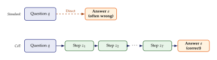
Reasoning Models
Chain-of-thought prompting demonstrates that LLMs can reason mathematically when guided to do so. But standard CoT relies on the user providing the right prompt, and the model has no incentive to produce correct reasoning chains. The next generation of models addresses this by training for extended reasoning. These reasoning models are explicitly optimized to generate long, accurate chains of thought, using reinforcement learning to reward correct final answers.
OpenAI o-Series Models
The OpenAI o-series, beginning with o1 in September 2024, represents a paradigm shift in how language models approach mathematical problems [112]. Rather than generating a response immediately, o-series models first produce an internal chain-of-thought (sometimes called “thinking tokens”) that is not shown to the user. Only after this internal reasoning phase does the model produce its final response.
Architecture and training.
The o-series models share the same underlying transformer architecture as GPT-4, but are fine-tuned using a specialized reinforcement learning pipeline:
Supervised fine-tuning on reasoning traces. The model is first trained on a curated dataset of mathematical problems paired with detailed, step-by-step solutions. These solutions include explicit reasoning steps, self-corrections, and verification steps.
Reinforcement learning with outcome-based rewards. The model is then trained with RL, where the reward signal is based solely on the correctness of the final answer. The model is free to develop any internal reasoning strategy that leads to correct answers. This is crucial: the reasoning process is not prescribed, only the outcome is rewarded.
Process reward models (PRMs). In addition to outcome-based rewards, o-series models use process reward models that evaluate individual reasoning steps. A PRM assigns a score to each step in the chain of thought, enabling more fine-grained credit assignment. The PRM is trained on human annotations of step-by-step correctness [35].
Performance characteristics.
The o1 model achieved 83.3% on the MATH benchmark (competition mathematics) at launch, compared to 52.9% for GPT-4. The o3 model, released in early 2025, pushed this to approximately 96%, approaching human expert performance. The o4-mini variant demonstrated that reasoning capabilities could be distilled into smaller models while retaining most of the mathematical performance, achieving around 93% on MATH with significantly lower latency [113].
Remark 21.
An important feature of o-series models is test-time compute scaling: the model can be given more “thinking time” (more tokens for internal reasoning) to solve harder problems. This creates a natural trade-off between computational cost and accuracy, analogous to the time-accuracy trade-off in iterative numerical methods.
GPT-5.4 Pro and beyond.
The GPT-5.4 Pro model, released in 2026, integrates reasoning capabilities directly into the base architecture rather than treating them as a fine-tuning overlay. This model achieves near-perfect scores on standard mathematical benchmarks (over 99% on GSM8K, 97% on MATH) and demonstrates novel capabilities on research-level problems from the FrontierMath benchmark [50]. The model can engage in multi-step mathematical research, generating conjectures, testing them against examples, and producing proof sketches, though its proofs still require human verification for correctness.
DeepSeek-R1: Open Reasoning
While the o-series models are proprietary, the DeepSeek-R1 model, released in January 2025, demonstrated that open-weight reasoning models could achieve comparable performance [114]. DeepSeek-R1 is particularly significant for the mathematical reasoning community because its training recipe is fully documented.
Training pipeline.
DeepSeek-R1 is trained in several stages:
Pre-training. The base model (DeepSeek-V3) is pre-trained on a large corpus including mathematical text, code, and scientific literature.
Cold-start supervised fine-tuning. A small set of high-quality reasoning traces (approximately 5,000 examples) is used to teach the model the format of step-by-step reasoning. These examples include explicit “thinking” sections demarcated by special tokens.
RL training with GRPO. The model is then trained using Group Relative Policy Optimization (GRPO), a reinforcement learning algorithm that we describe in detail in Group Relative Policy Optimization (GRPO). The reward signal combines: itemize
Correctness of the final answer (verified programmatically for math problems).
Format compliance (whether the response follows the expected structure). itemize
Rejection sampling and further SFT. The RL-trained model generates many solutions to a large problem set. Correct solutions are filtered and used for another round of supervised fine-tuning, which stabilizes the model's output quality.
Final RL round. A second round of GRPO training on a broader set of tasks ensures that the model's reasoning abilities generalize beyond mathematics to coding, science, and general question answering.
Emergent behaviours.
One of the most remarkable findings from DeepSeek-R1 training is the emergence of sophisticated reasoning behaviours that were never explicitly taught:
Self-verification: the model spontaneously learns to check its own work, re-deriving results from scratch to verify consistency.
Backtracking: when the model detects an error in its reasoning chain, it backtracks to an earlier step and tries a different approach.
Exploration: the model considers multiple solution strategies before committing to one, sometimes explicitly listing “Approach 1,” “Approach 2,” etc.
The “aha moment”: in some training runs, the model's chain-of-thought includes phrases like “Wait, let me reconsider” followed by a correction that leads to the right answer. This behaviour was not present in the cold-start data.
Historical Note.
The emergence of self-correction in DeepSeek-R1 echoes a long-standing debate in cognitive science about whether reasoning is a deliberate, sequential process (System 2 thinking in Kahneman's framework) or an automatic, pattern-matching process (System 1). DeepSeek-R1 suggests that System-2-like behaviours can emerge from System-1 architectures (autoregressive transformers) when trained with appropriate reinforcement signals [36].
Group Relative Policy Optimization (GRPO)
GRPO is the reinforcement learning algorithm at the heart of DeepSeek-Math and DeepSeek-R1. It was introduced specifically to address the challenges of RL training for mathematical reasoning [51]. To understand GRPO, we first review the standard RL framework for language model training, then identify the problem that GRPO solves, and finally present the algorithm in detail.
Background: RL for Language Models
The standard approach to RL fine-tuning of language models uses Proximal Policy Optimization (PPO) [115]. In this framework:
The policy is the language model parameterized by .
The action space is the vocabulary of the model.
A state at time is the concatenation of the prompt and the tokens generated so far: .
The reward is assigned to the complete response and is typically sparse: for a correct answer, or for incorrect.
The PPO objective for a single prompt is: (Objective) where is the importance ratio and is the estimated advantage function.
The value function problem.
The critical challenge in PPO for mathematical reasoning is estimating the advantage . Standard PPO uses a learned value function to estimate the expected future reward from state , and computes advantages via Generalized Advantage Estimation (GAE): (GAE) For mathematical reasoning, this approach has several problems:
Reward sparsity. The reward is typically given only at the end of the response, so most per-token rewards are zero. The value function must learn to propagate the final reward backward through potentially hundreds of tokens.
Value function size. The value function must be as large as the policy model to accurately estimate the expected return from complex mathematical states. This doubles the memory and computation requirements.
Non-stationarity. As the policy improves, the distribution of states changes, and the value function must be continuously retrained. In mathematical reasoning, the state distribution can shift rapidly (the model learns new strategies), causing the value function to lag.
Approximation error. Errors in the value function estimate propagate through the advantage computation, leading to noisy gradient signals that destabilize training.
The GRPO Algorithm
GRPO eliminates the learned value function entirely. Instead of estimating advantages from a value network, GRPO estimates advantages by sampling multiple responses to the same prompt and using their relative rewards.
Definition 17 (Group Relative Policy Optimization).
Given a prompt , sample complete responses from the current policy . Compute the reward for each response: for . The group-relative advantage for response is: (Advantage) where is a small constant for numerical stability. The GRPO objective is: (Objective) where is the per-token importance ratio for response , is the length of response , and the KL divergence term regularizes toward a reference policy .
Intuition.
The core idea is simple: among the responses to the same prompt, some will be correct and others incorrect. By normalizing rewards within the group, GRPO turns the sparse binary reward signal into a dense, informative advantage signal. Responses that are better than the group average receive positive advantage and are reinforced; responses that are worse receive negative advantage and are suppressed. No value function is needed because the group itself serves as a baseline.
Comparison with PPO.
| Feature | PPO | GRPO |
| Advantage estimation | Learned | Group normalization |
| Value network required | Yes | No |
| Memory overhead | policy | policy |
| Samples per prompt | 1 | (typically –) |
| Reward type | Per-token (via GAE) | Per-response |
| Training stability | Moderate | High |
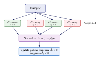
Theoretical Properties of GRPO
We now establish that GRPO, despite its simplicity, has desirable theoretical properties. The following theorem shows that the group-relative advantage is an unbiased estimator of the true advantage under mild conditions.
Theorem 10 (Unbiasedness of group-relative advantage).
Let be a prompt and let be the reward for response . Define the expected reward and the reward variance . Then the GRPO advantage estimate from (Advantage) satisfies: (Unbiased) That is, is an asymptotically unbiased estimator of the normalized advantage as .
Proof.
By the law of large numbers, and almost surely as . For finite , we have and . The sample mean includes itself, introducing a bias of order : conditional on , we have . Substituting into and using a Taylor expansion around , we obtain the stated result.
Theorem 11 (GRPO convergence).
Under the following conditions:
the reward function is bounded: ,
the clipping parameter satisfies ,
the KL coefficient satisfies ,
the group size satisfies ,
the GRPO objective converges to a stationary point of the regularized reward maximization problem: (Convergence) Moreover, the converged policy satisfies .
Proof sketch.
The proof follows the standard analysis of clipped policy gradient methods. The clipping ensures that the policy update is conservative (the ratio stays close to ). The KL regularization ensures that the objective is strongly concave in a neighborhood of , guaranteeing a unique global maximum. The group-relative advantage introduces additional variance compared to the true advantage, but this variance decreases as by Theorem 10, so the gradient estimate remains consistent. The converged policy is obtained by setting the gradient of the unclipped, unregularized version to zero and solving the resulting optimization problem with a Lagrange multiplier for the KL constraint.
Remark 22.
Theorem 11 shows that GRPO converges to the same optimal policy as PPO with a perfect value function: the Boltzmann policy . The advantage of GRPO is practical, not theoretical: it avoids the value function approximation errors that plague PPO in practice.
GRPO in Practice: DeepSeek-Math
DeepSeek-Math was the first model to demonstrate the effectiveness of GRPO for mathematical reasoning [51]. The model was trained on a curated mathematical corpus of approximately 120 billion tokens, spanning textbooks, competition problems, research papers, and mathematical web content.
Architecture.
DeepSeek-Math uses a standard transformer decoder architecture with 7 billion parameters. The pre-training corpus was specifically curated for mathematical content using a quality classifier trained to distinguish high-quality mathematical text from generic web content.
GRPO hyperparameters.
The key hyperparameters used in DeepSeek-Math training are:
Group size: (64 responses per prompt).
Clipping parameter: .
KL coefficient: .
Learning rate: with cosine decay.
Maximum response length: 2,048 tokens.
Training prompts: 144,000 mathematical problems.
Results.
DeepSeek-Math 7B achieved 51.7% on the MATH benchmark, matching GPT-4's performance at the time despite being roughly 200 times smaller. With GRPO fine-tuning on top of the pre-trained model, performance increased to 58.8%, demonstrating the effectiveness of RL-based training for mathematical reasoning.
Example 38 (GRPO training dynamics).
Consider a training prompt: “Find all integer solutions to .”
In an early training iteration, the model generates responses:
(incomplete)
(incomplete)
(correct)
(wrong)
Similar to response 3 (correct)
(incomplete)
(incomplete)
Similar to response 3 (correct)
Group statistics: , . The three correct responses receive advantage , while the five incorrect responses receive . GRPO reinforces the complete, correct responses and suppresses the incomplete ones.
Specialized Mathematical Language Models
Beyond reasoning-focused training, another approach to improving LLMs for mathematics is to curate the pre-training data itself. Google's Minerva model [116] demonstrated that training on a large corpus of scientific and mathematical text produces a model with significantly better mathematical reasoning than a general-purpose LLM of the same size.
Training data curation.
Minerva was based on PaLM (540B parameters) and further trained on a curated dataset of 38.5 billion tokens from scientific papers (from arXiv), mathematical web pages, and textbooks. The key innovation was the data processing pipeline:
LaTeX formulas were preserved in their original form rather than being rendered or stripped.
Mathematical notation was normalized to reduce ambiguity.
Low-quality or non-mathematical content was filtered using a classifier.
Results.
Minerva 540B achieved 50.3% on the MATH benchmark and 78.5% on GSM8K at the time of publication (mid-2022), which were state-of-the-art results. Importantly, Minerva used majority-vote sampling (generating multiple solutions and taking the most common answer), which improved performance significantly over single-sample inference.
Subsequent models.
The landscape of mathematical LLMs has expanded rapidly since Minerva. Notable models include:
Llemma [37]: an open-source mathematical LLM trained on the Proof Pile II dataset, which includes mathematical code (Lean, Isabelle) alongside natural-language mathematics.
InternLM-Math [38]: which combines chain-of-thought reasoning with tool use (calling Python and Lean) for verified mathematical problem solving.
Qwen-Math [39]: which achieves strong mathematical performance through a combination of pre-training data curation and GRPO-style RL training.
Mathematical Benchmarks and the Progress Curve
The rapid progress in LLM-based mathematical reasoning is best measured through standardized benchmarks. We survey the major benchmarks, their characteristics, and the trajectory of performance improvement from 2022 to 2026.
GSM8K: Grade School Math
GSM8K (Grade School Math 8K) is a dataset of 8,792 grade-school level math word problems requiring basic arithmetic and multi-step reasoning [117]. Each problem requires 2–8 steps of elementary operations (addition, subtraction, multiplication, division) embedded in a natural language context.
Example 39 (GSM8K problem).
Problem: Natalia sold clips to 48 of her friends in April, and then she sold half as many clips in May. How many clips did Natalia sell altogether in April and May?
Solution: Natalia sold clips in May. Natalia sold clips altogether in April and May. The answer is .
GSM8K performance has risen from approximately 57% (GPT-3, few-shot CoT) in 2022 to over 99% (GPT-5.4 Pro) in 2026. The benchmark is now considered essentially solved for frontier models.
MATH: Competition Mathematics
The MATH benchmark [118] contains 12,500 competition-level mathematics problems drawn from AMC, AIME, and Olympiad competitions. Problems span seven subject areas: algebra, counting and probability, geometry, intermediate algebra, number theory, prealgebra, and precalculus. Each problem is assigned a difficulty level from 1 (easiest) to 5 (hardest).
Example 40 (MATH benchmark problem (Level 4)).
Problem: Let and be positive real numbers such that . Find the minimum value of .
Solution: By the AM-HM inequality, . Since , we get , so . Equality holds when . The minimum value is .
MATH benchmark performance has risen from approximately 6.9% (GPT-3) in 2022 to approximately 97% (GPT-5.4 Pro) in 2026. Level-5 problems remain the most challenging, with error rates roughly 5 times higher than Level-1 problems even for the best models.
FrontierMath: Research-Level Problems
FrontierMath is a benchmark of research-level mathematics problems developed in collaboration with professional mathematicians [50]. Unlike GSM8K and MATH, which test well-studied problem types, FrontierMath problems require novel mathematical insight and multi-hour reasoning.
Characteristics of FrontierMath problems.
Problems are drawn from active research areas: algebraic geometry, analytic number theory, combinatorics, differential equations, and more.
Each problem was created by a professional mathematician and has a verified numerical answer.
Problems require multiple insights, typically taking expert mathematicians several hours to solve.
The benchmark is “guessproof”: answers are large integers or fractions that cannot be guessed by pattern matching.
As of early 2026, even the most capable models solve fewer than 10% of FrontierMath problems, making it a key benchmark for measuring future progress.
MiniF2F: Formal Mathematics
MiniF2F is a benchmark of 488 mathematical statements formalized in multiple theorem provers (Lean, Isabelle, Metamath) [119]. The task is to produce a complete, machine-verifiable proof of each statement. Unlike other benchmarks, MiniF2F has no ambiguity: a proof is either accepted by the proof checker or it is not.
MiniF2F performance has risen from approximately 29% (initial neural approaches) to approximately 55% (AlphaProof-style systems) as of 2025. The benchmark remains challenging because it requires both mathematical insight and fluency in formal proof languages.
The Progress Curve
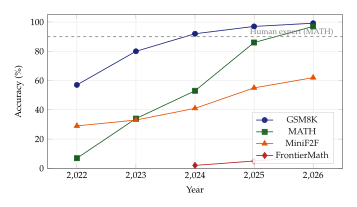
The progress curve reveals several important patterns:
Benchmark saturation. GSM8K saturated by 2025, illustrating the need for increasingly difficult benchmarks.
Diminishing returns on easy problems. The gains on GSM8K slowed as accuracy approached 100%, while gains on harder benchmarks (MATH, FrontierMath) accelerated.
The formal verification gap. MiniF2F progress has been slower than informal mathematical reasoning, suggesting that generating formal proofs remains significantly harder than generating informal solutions.
The research frontier. FrontierMath performance below 10% shows that current models cannot yet do novel mathematical research, even with extended reasoning.
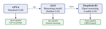
Exercises
Exercise 48 (Chain-of-thought decomposition).
Consider the problem: “A farmer has chickens and cows. She counts 30 heads and 80 legs. How many chickens and how many cows does she have?”
Write a chain-of-thought solution that decomposes the problem into elementary steps.
Identify the minimum number of intermediate tokens needed for a transformer to solve this problem with CoT. Justify your answer.
Can this problem be solved without CoT by a sufficiently large transformer? What would the circuit need to compute?
Exercise 49 (GRPO implementation).
Suppose you have a language model policy and a reward function (correct/incorrect).
For responses to a prompt, suppose 3 are correct and 5 are incorrect. Compute the GRPO advantages for each response.
Show that the gradient of the GRPO objective pushes the policy to increase the probability of correct responses and decrease the probability of incorrect ones.
What happens when (a single response)? Why is this a degenerate case?
Derive the optimal group size that minimizes the variance of the gradient estimator, assuming the reward is Bernoulli with parameter (the model's accuracy).
Exercise 50 (Computational power of CoT).
Show that a transformer with CoT of length can sort a list of numbers. Describe the algorithm that the CoT tokens would encode.
Prove that without CoT, a constant-depth transformer cannot compute the parity function on bits (i.e., whether the number of 1s is even or odd). Hint: Use the fact that and for this specific function.
Design a CoT strategy for computing using the Euclidean algorithm. How many CoT tokens are needed as a function of ?
Exercise 51 (Benchmark analysis).
A model achieves 95% on MATH Level 1–3 problems but only 40% on Level 4–5 problems. Compute the overall MATH accuracy if 60% of problems are Level 1–3 and 40% are Level 4–5.
If a model's accuracy on MATH improves by 10 percentage points per year (linear extrapolation), when would it reach 100%? Why is linear extrapolation likely inaccurate?
A FrontierMath problem has a numerical answer that is a 10-digit integer. What is the probability of guessing it correctly at random? Why does this make FrontierMath “guessproof”?
Exercise 52 (Value function vs. group normalization).
Consider a simplified setting where the reward is binary () and the model's current accuracy is (it gets 30% of problems correct).
For PPO with a perfect value function, what is the advantage of a correct response? What is the advantage of an incorrect response?
For GRPO with , compute the expected advantage of a correct response. How does it compare to the PPO case?
Now suppose the value function has 20% error (it estimates instead of ). How does this affect the PPO advantages? How does GRPO avoid this issue?
From Natural Language to Formal Proofs: Autoformalization
Mathematics lives in two worlds. In the informal world, mathematicians write proofs in natural language sprinkled with notation, relying on shared intuition, implicit context, and the reader's ability to fill in gaps. In the formal world, every statement, every inference rule, and every logical step is made explicit in a language that a computer can verify.
The dream of autoformalization is to build a bridge between these two worlds: to automatically translate the vast body of informal mathematics, textbooks, papers, competition solutions, lecture notes, into machine-verifiable formal proofs [75]. If realized, this dream would unlock an enormous training signal for AI systems (since formal proofs can be verified automatically), accelerate the formalization of mathematical knowledge, and create a new mode of human-AI collaboration in mathematics.
Key Idea.
Autoformalization is the task of translating informal mathematical text (theorems, proofs, definitions) into formal representations that can be verified by a proof assistant. It is one of the most important open problems at the intersection of AI and mathematics, because success would create a virtually unlimited source of verified training data.
Why Autoformalization Is Hard
Before examining solutions, we must understand why autoformalization is so difficult. The gap between informal and formal mathematics is not a simple notational difference; it reflects fundamentally different modes of mathematical communication.
Ambiguity of mathematical language.
Informal mathematics is rife with ambiguity. Consider the statement “Let be a continuous function.” In Lean 4, we must specify:
The domain and codomain of (e.g., ).
The topology on each (e.g., the standard metric topology).
The precise definition of continuity being used (epsilon-delta, sequential, topological).
The informal statement leaves all of this implicit, relying on context that a human reader can infer but a machine cannot.
Notation overloading.
Mathematical notation is heavily overloaded. The symbol “” can mean integer addition, real addition, vector addition, matrix addition, concatenation, or the join operation in a lattice, depending on context. The expression can mean the absolute value, the norm, the cardinality, or the determinant. A formalization system must resolve every such ambiguity.
Implicit knowledge.
Mathematicians routinely omit steps that they consider “obvious.” A typical informal proof might say “by a simple counting argument” or “it follows from standard results in linear algebra.” Formalizing such steps requires the system to identify the relevant lemmas, instantiate them with the correct arguments, and chain them together into a valid proof.
Library dependence.
Formal proofs do not exist in isolation. Every formal statement depends on a library of previously formalized definitions and lemmas. Lean's Mathlib, for example, contains over 150,000 declarations [67]. Autoformalization must map informal concepts to the correct library entities, which may use different names, different conventions, or different levels of generality than the informal text.
Example 41 (Autoformalization difficulty levels).
Easy. “”
theorem : 2 + 3 = 5 := by norm_num. Almost no ambiguity; direct translation.Medium. “The sum of two even numbers is even.” Requires choosing a formalization of “even” (
Even nin Mathlib), universally quantifying over the two numbers, and proving the result.Hard. “Every finite group of prime order is cyclic.” Requires group theory definitions, the concept of prime order, the definition of cyclic groups, and Lagrange's theorem, a proof that touches multiple parts of the library.
Very hard. A competition problem involving a combination of algebra, number theory, and combinatorics. The formalization requires choosing appropriate abstractions, may not map cleanly to existing library concepts, and the proof itself may require novel combinations of tactics.
Early Approaches to Autoformalization
Before the advent of large language models, autoformalization was pursued through rule-based and pattern-matching approaches.
Controlled natural language.
The earliest approach was to restrict the input to a controlled natural language (CNL) that is close enough to formal logic for deterministic parsing. The Mizar system uses a CNL that reads like stilted English but has a precise formal semantics [60]. The Naproche (Natural Proof Checking) project extends this idea by parsing a carefully structured subset of mathematical English [120].
Remark 23.
Controlled natural languages achieve high precision (most translations are correct) at the cost of expressiveness: mathematicians must write in an unnatural style that resembles a programming language more than mathematical prose. This severely limits adoption.
Pattern matching and templates.
Another early approach uses pattern matching to identify common mathematical constructions and map them to formal templates. For example, the pattern “for all such that , we have ” maps to the formal template . While effective for simple statements, this approach cannot handle the rich variety of mathematical expression.
Semantic parsing.
Semantic parsing techniques from natural language processing have been applied to mathematical text, treating formalization as a translation problem from natural language to a formal target language [121]. These approaches use grammars that capture the syntactic structure of mathematical statements and produce formal output. However, they struggle with the long-range dependencies and implicit context that characterize real mathematical writing.
LLM-Based Autoformalization
The application of large language models to autoformalization represents a paradigm shift. Instead of hand-crafting rules or templates, LLMs learn to translate between informal and formal mathematics from examples, leveraging their broad understanding of both natural language and formal notation.
GPT-4 for Informal-to-Lean Translation
Wu et al. demonstrated that GPT-4, without any fine-tuning, could translate informal mathematical statements into Lean 4 code with moderate success [75]. The approach is straightforward: provide the model with a prompt containing the informal statement, a few examples of informal-to-formal translations, and ask it to produce the Lean formalization.
Example 42 (GPT-4 autoformalization).
Informal: “The sum of two even numbers is even.”
Prompt: Translate the following mathematical statement into Lean 4 code. Use Mathlib definitions where appropriate.
GPT-4 output:
theorem even_add_even (m n : Nat)
(hm : Even m) (hn : Even n) : Even (m + n) := by
obtain <hk, rfl> := hm
obtain <hl, rfl> := hn
exact <hk + hl, by ring>
Result: This proof compiles and is verified by
Lean 4. The model correctly identified the Mathlib
Even predicate, used appropriate tactics, and produced
a valid proof.
Success rates.
In initial evaluations, GPT-4 successfully formalized approximately 35% of informal statements from a test set of competition-level mathematics problems. The primary failure modes were:
Incorrect library references (using Mathlib functions that do not exist).
Type mismatches (confusing natural numbers with integers or reals).
Incomplete proofs (generating proof sketches that do not compile).
Hallucinated tactics (inventing Lean tactics that are syntactically plausible but do not exist).
ProofGPT and Dedicated Proof Models
While general-purpose LLMs show promise, dedicated models trained specifically on formal mathematics perform significantly better. ProofGPT [37] and related models are trained on large corpora of formal proofs, learning the syntax, idioms, and proof strategies of specific proof assistants.
Training data.
Dedicated proof models are typically trained on:
The entire Mathlib library (for Lean-focused models).
The Archive of Formal Proofs (for Isabelle-focused models).
Synthetic data generated by applying tactics to random goals and recording the results.
Human-annotated pairs of informal statements and their formalizations.
Architecture.
Most proof generation models use a standard transformer decoder architecture, but with several adaptations:
Proof state conditioning: the model receives the current proof state (the list of goals and hypotheses in the proof context) as input, not just the theorem statement.
Tactic generation: rather than generating an entire proof at once, the model generates one tactic at a time, and the proof assistant executes the tactic and returns the updated proof state.
Tree search: the model's predictions are combined with a search algorithm (beam search, best-first search, or Monte Carlo tree search) that explores multiple proof paths and backtracks when a tactic fails.
Draft, Sketch, Prove
The Draft, Sketch, Prove (DSP) framework decomposes autoformalization into three stages, each more amenable to automation than direct end-to-end translation [122]:
Draft: an LLM generates an informal proof of the given theorem in natural language. This step leverages the model's mathematical reasoning ability without requiring formal output.
Sketch: a second LLM (or the same model with a different prompt) translates the informal proof into a formal proof sketch: a sequence of intermediate lemmas and proof steps in the formal language, with some steps left as “sorry” (unproved placeholders).
Prove: an automated tactic prover fills in the “sorry” placeholders, converting the sketch into a complete formal proof. This step uses existing tactic automation (e.g., Lean's
omega,norm_num,simp) and neural tactic prediction.
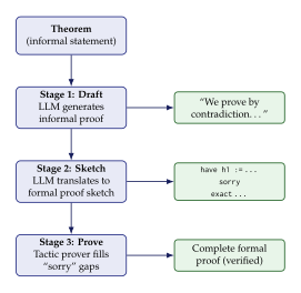
Results.
DSP improved the success rate on MiniF2F from 33.6% (direct neural proof generation) to 42.6%, a significant improvement that demonstrated the value of decomposing the formalization task. The key insight is that informal proofs, while not directly useful for verification, provide a proof plan that guides the formal proof search.
The Two-Way Bridge
Autoformalization is not a one-way street. The reverse direction, informalization (converting formal proofs into readable natural-language explanations), is equally important and, as it turns out, significantly easier.
Formalization: Informal to Formal
The forward direction (informal formal) is the harder task. It requires the system to:
Parse the intent of the informal text.
Resolve all ambiguities.
Map concepts to library definitions.
Generate a syntactically and logically correct formal proof.
Current success rates range from 35% (GPT-4, zero-shot) to approximately 55% (specialized systems with search), depending on the difficulty of the problems.
Informalization: Formal to Informal
The reverse direction (formal informal) is easier because formal proofs contain all the information needed; the task is merely to present it in a human-readable form. LLMs are particularly good at this: given a formal Lean proof, they can produce a clear, step-by-step natural language explanation.
Example 43 (Informalization of a Lean proof).
Formal (Lean 4):
theorem sqrt2_irrational : Irrational (Real.sqrt 2) := by
rw [Real.irrational_sqrt_iff (by norm_num : (0:R) <= 2)]
exact Nat.Prime.irrational_sqrt (by norm_num : Nat.Prime 2)
LLM-generated informal version:
The informal version is not only correct but also more readable than the formal proof, demonstrating the value of informalization for mathematical education and communication.Theorem: is irrational.
Proof: We use the fact that for any non-negative real number , is irrational if and only if is not a perfect square. Since is a prime number, it is not a perfect square, and therefore is irrational.
Applications of informalization.
Education: explaining formal proofs to students learning proof assistants.
Documentation: automatically generating documentation for formal mathematics libraries.
Verification: mathematicians can read the informal explanation to check that the formal proof captures their intended argument.
Training data generation: informalized proofs can be used as training data for autoformalization (see Synthetic Data Generation for Autoformalization).
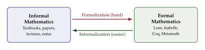
Synthetic Data Generation for Autoformalization
A major bottleneck in training autoformalization systems is the scarcity of paired (informal, formal) data. While there are millions of informal mathematical texts and thousands of formal proofs, the number of aligned pairs where the same mathematical content exists in both forms is small.
The back-translation approach.
The most successful strategy for generating training data borrows the back-translation technique from machine translation [123]. The idea is:
Start with a large corpus of formal proofs (e.g., Mathlib).
Use an LLM to informalize each formal proof, generating a natural-language description.
Use the resulting (informal, formal) pairs to train an autoformalization model.
Use the trained model to formalize new informal texts, check which formalizations are correct (using the proof checker), and add correct pairs to the training set.
Iterate.
This creates a virtuous cycle: better informalization produces better training data, which produces better formalization, which produces more verified pairs.
Synthetic proof generation.
An alternative approach generates entirely synthetic formal proofs by:
Randomly composing library lemmas to create new theorems.
Using tactic automation to prove random goals.
Perturbing existing proofs (changing variable names, reordering steps, generalizing statements).
Each synthetic proof is then informalized by an LLM to create training pairs. This approach can generate virtually unlimited training data, though the quality and diversity of the synthetic proofs may be limited.
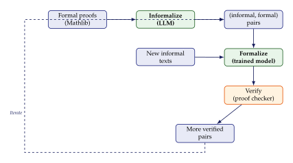
Detailed Examples of Autoformalization
We present three detailed examples of autoformalization at increasing difficulty levels, illustrating both the capabilities and limitations of current systems.
Simple: Even Number Addition
Informal statement: “The sum of two even numbers is even.”
Formal statement (Lean 4):
theorem even_add_even (m n : Nat)
(hm : Even m) (hn : Even n) : Even (m + n) := by
obtain <hk, rfl> := hm
obtain <hl, rfl> := hn
exact <hk + hl, by ring>
Analysis.
This example is straightforward because:
The informal statement has minimal ambiguity (“even” has a standard definition).
The proof is short and uses only basic tactics.
The Mathlib
Evenpredicate directly matches the informal concept.
Current LLMs succeed on this type of problem approximately 80% of the time.
Medium: Cyclic Groups of Prime Order
Informal statement: “Every finite group of prime order is cyclic.”
Formal statement (Lean 4):
theorem prime_order_cyclic {G : Type*} [Group G]
[Fintype G] (hp : Nat.Prime (Fintype.card G)) :
IsCyclic G := by
haveI := Fintype.one_lt_card_iff_nontrivial.mp
(hp.one_lt)
exact isCyclic_of_prime_card hp
Analysis.
This example is more challenging because:
The formalization requires knowing the Mathlib type class hierarchy (
Group,Fintype,IsCyclic).The proof relies on the library lemma
isCyclic_of_prime_card, which the model must identify.The informal statement says “finite group of prime order” which must be decomposed into the
Fintypeinstance and the condition onFintype.card.
Current LLMs succeed on this type of problem approximately 40% of the time. The most common failure is hallucinating library lemma names.
Hard: A Competition Problem
Informal problem (AMC-style): “Prove that for all positive integers , the number is divisible by 6.”
Informal proof: We factor: , which is the product of three consecutive integers. Among any three consecutive integers, one is divisible by 3 and at least one is divisible by 2, so the product is divisible by 6.
Formal proof (Lean 4):
theorem cube_minus_self_div6 (n : Nat) (hn : 0 < n) :
6 | (n^3 - n) := by
have h : n^3 - n = (n - 1) * n * (n + 1) := by ring
rw [h]
have h2 : 2 | (n - 1) * n * (n + 1) := by
rcases Nat.even_or_odd n with he | ho
. exact dvd_mul_of_dvd_left
(dvd_mul_of_dvd_right he.two_dvd _) _
. exact dvd_mul_of_dvd_left
(dvd_mul_of_dvd_left
(ho.sub_one_even.two_dvd) _) _
have h3 : 3 | (n - 1) * n * (n + 1) := by
omega
exact Nat.Coprime.mul_dvd_of_dvd_of_dvd
(by norm_num) h2 h3
Analysis.
This example is hard because:
The informal proof uses the concept of “consecutive integers” which must be translated into specific divisibility arguments.
The formal proof requires case analysis on the parity of and reasoning about divisibility by 3.
The
ringtactic handles algebraic simplification, but the divisibility arguments require more sophisticated reasoning.The model must combine multiple library lemmas (
Nat.even_or_odd,dvd_mul_of_dvd_left,Nat.Coprime.mul_dvd_of_dvd_of_dvd) in the correct way.
Current LLMs succeed on problems of this difficulty approximately 15–25% of the time with search-based approaches.
Current Success Rates and Limitations
We summarize the current state of autoformalization performance across different difficulty levels and approaches.
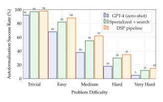
Key limitations.
Despite impressive progress, autoformalization faces several fundamental limitations:
Library coupling. Autoformalization performance is tightly coupled to the formal library being used. A model trained for Lean/Mathlib cannot easily transfer to Isabelle/AFP or Coq/MathComp. Each library has its own conventions, naming schemes, and proof idioms.
Novel mathematics. Current systems struggle with mathematics that goes beyond the library, i.e., theorems that require new definitions or techniques not present in the training data. This is the most significant barrier to using autoformalization for research-level mathematics.
Proof length. Success rates drop sharply with proof length. Proofs requiring more than 50 lines of formal code are rarely generated correctly, because errors compound across steps.
Verification overhead. While formal proofs can be verified automatically, the verification itself can be slow (some Lean proofs take minutes to check), creating a bottleneck in search-based approaches that must verify many candidate proofs.
Mathematical creativity. Autoformalization is fundamentally a translation task: it converts an existing informal argument into formal language. It does not (yet) involve the creative step of discovering the proof in the first place. Systems like AlphaProof address this complementary challenge (AlphaProof: DeepMind's IMO Solver).
Remark 24.
The gap between formalization and informalization success rates is striking. While informalization succeeds approximately 90% of the time across all difficulty levels (since the formal proof contains all necessary information), formalization success drops below 50% for problems beyond the “easy” category. This asymmetry suggests that the primary challenge is not understanding mathematics but resolving the ambiguity and implicit knowledge in informal text.
The Autoformalization Pipeline in Practice
We now describe a complete autoformalization pipeline that integrates the techniques discussed in this section into a practical system.
Definition 18 (Autoformalization pipeline).
An autoformalization pipeline consists of the following components:
Parser: extracts mathematical statements and proofs from informal text (LaTeX, PDF, or plain text).
Statement formalizer: translates informal theorem statements into formal type signatures.
Proof planner: generates a high-level proof plan (either from an informal proof or from scratch using chain-of-thought).
Tactic generator: converts the proof plan into a sequence of formal tactics.
Proof checker: verifies the generated proof using the proof assistant's kernel.
Repair module: when the proof checker reports errors, attempts to fix them (e.g., by trying alternative tactics or backtracking).
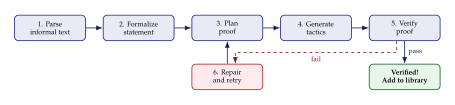
Integration with proof assistants.
Modern autoformalization systems interact with proof assistants
through a programmatic interface. In Lean 4, the
lean4-repl server provides an API for:
Submitting partial proofs and receiving the current proof state (goals and hypotheses).
Executing individual tactics and observing their effects.
Checking whether a proof is complete.
Reporting type errors and tactic failures with diagnostic information.
This allows the autoformalization system to operate in a feedback loop: generate a tactic, observe the result, and decide the next tactic based on the updated proof state.
Exercises
Exercise 53 (Ambiguity resolution).
Consider the informal statement: “ is a smooth function.”
List at least three different formal interpretations of this statement, specifying the domain, codomain, and differentiability class.
For each interpretation, write the corresponding Lean 4 type signature (you may use pseudo-code if you are not familiar with Lean syntax).
Propose a strategy for an autoformalization system to disambiguate this statement using context from the surrounding text.
Exercise 54 (Back-translation quality).
Consider a formal proof of “” for natural numbers. Write two different informalizations of this proof: one that is technically correct but unnatural (“by commutativity of addition in the natural numbers under the Peano axioms”), and one that is natural but technically imprecise (“clearly, addition is commutative”).
Which informalization would be more useful for training an autoformalization system? Justify your answer.
Design a scoring function that measures the quality of an informalization for use as training data. What properties should it reward?
Exercise 55 (DSP decomposition).
Consider the theorem: “The composition of two continuous functions is continuous.”
Write an informal proof (the “Draft” stage).
Convert your proof into a formal sketch with “sorry” placeholders (the “Sketch” stage). Identify which steps would need to be filled in by automated tactics.
For each “sorry” placeholder, describe what tactic or combination of tactics would be needed to fill it in (the “Prove” stage).
Exercise 56 (Autoformalization error analysis).
A model attempts to formalize “For all , we have .” The model produces:
theorem sum_formula (n : Nat) (hn : 1 <= n) :
Finset.sum (Finset.range n) id
= n * (n + 1) / 2 := by
sorry
Identify at least two errors in this formalization. Hint: consider the range of summation and the type of division.
Write a corrected version.
Explain why integer division makes this formalization trickier than it appears.
Exercise 57 (Synthetic data generation).
Design a procedure for generating synthetic formal theorems by composing library lemmas. Specifically, given two lemmas and , how would you automatically generate the theorem and its proof?
What quality control measures would you apply to ensure that the generated theorems are “interesting” (not trivially true or vacuously satisfied)?
Estimate the number of synthetic training pairs that could be generated from a library with 150,000 lemmas, assuming each pair of composable lemmas generates one training example.
Exercise 58 (Formalization difficulty prediction).
Propose a set of features (at least five) that could be used to predict the difficulty of formalizing an informal mathematical statement. Examples might include: statement length, number of mathematical symbols, presence of quantifiers, etc.
Using these features, design a simple classifier (e.g., logistic regression) that predicts whether autoformalization will succeed or fail.
How could such a difficulty predictor be used to improve the efficiency of an autoformalization pipeline?
Outlook: Toward Fully Automated Formalization
The field of autoformalization is evolving rapidly, and several emerging directions promise to narrow the gap between informal and formal mathematics.
Multi-modal formalization.
Mathematical texts often contain diagrams, graphs, and visual elements that carry essential information. A triangle in a geometry proof, a commutative diagram in algebra, or a visualization of a function all convey mathematical content that is absent from the text alone. Future autoformalization systems will need to process these visual elements alongside the text, requiring multi-modal architectures that can reason about both natural language and spatial/geometric content.
Interactive autoformalization.
Rather than attempting to formalize mathematics in a single pass, future systems may operate interactively, engaging in a dialogue with the mathematician. When the system encounters an ambiguity it cannot resolve, it asks for clarification. When it generates a formalization, it presents it to the user for feedback. This human-in-the-loop approach could dramatically improve success rates on hard problems while keeping the human effort manageable.
Curriculum learning for formalization.
Training autoformalization models on problems of increasing difficulty, starting with trivial translations and progressively moving to harder ones, mirrors the way human mathematicians learn formal proof assistants. Preliminary experiments suggest that curriculum learning improves both the final accuracy and the sample efficiency of autoformalization training.
Cross-library transfer.
Current autoformalization systems are tightly coupled to a single proof assistant and its library. Developing methods for transferring formalization knowledge across proof assistants (e.g., from Lean to Isabelle) would greatly expand the applicability of autoformalization. This requires learning abstract mathematical concepts that transcend any particular formal representation.
Historical Note.
The vision of formalizing all of mathematics dates back to Bertrand Russell and Alfred North Whitehead's Principia Mathematica (1910–1913), which attempted to derive all of mathematics from logical axioms using a formal system [40]. While their project was ultimately limited by Gödel's incompleteness theorems (1931) [41], the dream persists in modern form. The QED Manifesto (1994) called for a comprehensive computer-checked library of all important mathematical knowledge [42]. Three decades later, autoformalization powered by large language models offers the first realistic path toward realizing this vision, not by replacing human mathematicians but by dramatically reducing the effort required to formalize their work.
Key Idea.
The long-term significance of autoformalization extends beyond mathematics itself. If we can build systems that reliably translate informal reasoning into formally verified arguments, the same technology could be applied to software verification, legal reasoning, scientific hypothesis testing, and any domain where the correctness of reasoning matters. Mathematics is the ideal testbed because it has the clearest notion of “correct.”
Neural Theorem Proving: LLMs as Proof Assistants
The previous sections of this chapter explored how generative models can produce mathematical conjectures, solve word problems, and reason about symbolic expressions. But there is a qualitative difference between generating a plausible-looking proof sketch in natural language and producing a machine-verified proof in a formal proof assistant such as Lean, Coq, or Isabelle [13]. The former is subject to all the hallucination pathologies we have documented: the model may skip steps, invoke nonexistent theorems, or produce reasoning that looks convincing but is subtly wrong. The latter is either correct or it is not. The proof kernel accepts or rejects. There is no middle ground.
This binary verdict makes formal theorem proving an extraordinarily attractive target for generative models. Unlike natural language generation, where evaluation is fuzzy and subjective, formal theorem proving provides a perfect oracle: the type checker. A generated proof is correct if and only if the proof assistant accepts it. This eliminates the evaluation bottleneck that plagues most generative modelling tasks and, as we shall see in The Role of Reinforcement Learning in Mathematical Reasoning, provides an ideal reward signal for reinforcement learning.
Key Idea.
Formal theorem proving is the gold standard for AI-assisted mathematics because it combines two desirable properties: (1) the search space is rich enough to require genuine mathematical reasoning, and (2) correctness is mechanically verifiable by the proof kernel. No other domain offers such a clean interface between generation and verification.
The challenge, of course, is that formal proofs are difficult to write. Even experienced mathematicians find the translation from informal reasoning to formal proof code tedious and time-consuming [124]. The gap between “I see why this is true” and “here is a sequence of tactics that Lean accepts” is enormous. This gap is precisely where neural theorem provers operate: they generate tactic suggestions that the human (or an automated search procedure) can use to close proof goals.
In this section, we survey the rapidly growing ecosystem of neural theorem proving systems, with a focus on those that target the Lean proof assistant [13]. We begin with LeanDojo [125], which established the infrastructure for extracting training data from Lean repositories. We then discuss Lean Copilot [126], which brings neural tactic suggestion directly into the editor. We continue with LeanAgent [127], which introduces lifelong learning for theorem proving, and LeanProgress [128], which uses proof progress prediction to guide search. We cover APOLLO [129], a multi-agent collaboration framework, and TheoremLlama [130], which fine-tunes open-source LLMs into Lean experts. We conclude with a comparative table and a discussion of the neural theorem proving pipeline.
LeanDojo: Theorem Proving with Retrieval-Augmented Language Models
The fundamental bottleneck in applying machine learning to formal theorem proving has historically been data. Formal proof repositories such as Mathlib [131] contain tens of thousands of theorems, but extracting training data from them is nontrivial. A Lean proof is not a flat sequence of tokens: it is an interaction trace between the user and the proof kernel, where each tactic transforms a proof state (a set of goals with hypotheses) into a new proof state. To train a tactic prediction model, one needs (proof state, tactic) pairs, and extracting these requires instrumenting the Lean compiler to record the intermediate states.
LeanDojo [125] solves this problem with an open-source toolchain that can:
Extract interaction traces from any Lean 4 repository, producing (proof state, tactic, next proof state) triples along with the full dependency graph of the repository.
Construct a benchmark of 98,734 theorems and proofs from Mathlib, split into training, validation, and test sets with careful attention to avoiding data leakage (theorems in the test set do not appear as premises in the training set).
Interact programmatically with the Lean proof kernel, allowing an external agent to submit tactics and observe the resulting proof state, much like a gym environment for reinforcement learning.
Architecture of LeanDojo
The LeanDojo system consists of three main components, illustrated in Figure 45.
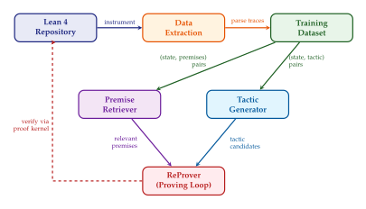
Data extraction.
The extraction pipeline instruments the Lean 4 compiler to record, for every tactic invocation in a repository, the proof state before the tactic, the tactic itself, and the proof state after the tactic. It also records the premises used by each tactic: which lemmas, definitions, and theorems from the library were referenced. This premise information is critical for the retrieval component.
The extraction is non-trivial because Lean 4 uses a sophisticated elaboration pipeline. A single user-written tactic may expand into dozens of internal kernel steps. LeanDojo traces the elaboration at the appropriate level of abstraction, producing data that is close to what a human user would write rather than the low-level kernel representation.
The LeanDojo Benchmark.
From Mathlib (the community-maintained mathematics library for Lean 4), LeanDojo extracts 98,734 theorems with their complete proof traces. The benchmark is split into three test configurations:
Random split: theorems are randomly assigned to train/validation/test sets.
Novel premises split: theorems in the test set use at least one premise not seen during training, testing generalisation to new mathematical concepts.
Novel file split: theorems in the test set come from files not present in the training data, testing generalisation to entirely new mathematical topics.
The novel premises split is particularly important because it measures the system's ability to work with mathematical concepts it has never encountered during training, a capability essential for proving genuinely new theorems rather than reproving variations of known results.
ReProver: Retrieval-Augmented Proving
The centrepiece of LeanDojo is ReProver (Retrieval-augmented Prover), a neural theorem prover that combines premise retrieval with tactic generation.
Premise retrieval.
Given a proof state , the retriever must identify which of the thousands of lemmas, definitions, and theorems in the library are relevant. ReProver uses a dense retrieval model based on a pretrained Transformer encoder. The proof state and each candidate premise are encoded independently: (Reprover Retrieval) where and are learned encoders. The model is trained with a contrastive loss that pushes the representations of a proof state and its actually-used premises closer together while pushing apart irrelevant premises.
Tactic generation.
Given the proof state and the top- retrieved premises , the tactic generator produces a tactic autoregressively: (Reprover Tacgen) The generator is a sequence-to-sequence Transformer (specifically, a fine-tuned ByT5 model [132]) that takes as input the concatenation of the proof state and the retrieved premises, and outputs a tactic token by token.
Best-first search.
At proving time, ReProver uses best-first search to explore the proof tree. At each step, it selects the most promising open goal (ranked by the cumulative log-probability of the tactics used to reach it), generates multiple tactic candidates, submits each to the Lean kernel, and adds the resulting proof states to the search frontier. The search terminates when all goals are closed (success) or a computational budget is exceeded (failure).
Definition 19 (Best-First Proof Search).
Let be the set of open goals. For each goal , compute a priority score , where is the sequence of tactics from the root to . Select , generate tactic candidates for , verify each with the proof kernel, and update accordingly.
Results.
On the LeanDojo Benchmark random split, ReProver achieves a pass rate of approximately 51.2%, substantially outperforming prior methods based on GPT-4 (which achieves roughly 29% on the same split when used in a zero-shot tactic suggestion mode). On the more challenging novel premises split, ReProver achieves 25.4%, demonstrating a meaningful ability to generalise to unseen mathematical concepts.
Remark 25.
The retrieval component of ReProver is essential. Without it (i.e., using only the tactic generator with no premise information), performance drops by approximately 10 percentage points on the random split. This confirms the intuition that knowing which lemmas to use is a critical bottleneck in theorem proving, not just knowing which tactic to apply.
Lean Copilot: LLMs as Copilots for Theorem Proving
While LeanDojo focuses on fully automated theorem proving, many mathematicians are more interested in a collaborative workflow: they want to write proofs themselves, with an AI assistant suggesting tactics, filling in tedious steps, and pointing out useful lemmas. This is the design philosophy of Lean Copilot [126], which integrates neural tactic suggestion directly into the Lean 4 editor (VS Code with the Lean extension).
Integration Architecture
Lean Copilot operates as a Lean 4 plugin that communicates with an external language model server. When the user positions their cursor at a proof step, the plugin extracts the current proof state (goals and hypotheses) and sends it to the language model. The model returns one or more tactic suggestions, which are displayed inline in the editor. The user can accept a suggestion with a single keystroke, at which point the Lean kernel immediately verifies it. If verification fails, the suggestion is silently discarded and the next candidate is presented.
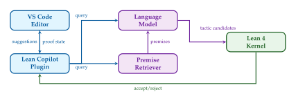
Three Modes of Operation
Lean Copilot provides three complementary modes of interaction:
Mode 1: Suggest next tactic.
Given the current proof state, the model suggests one or more tactics that might make progress. This is the most common mode and corresponds to the tactic prediction task studied in LeanDojo. The suggestions appear as ghost text in the editor, much like GitHub Copilot suggestions for code.
Mode 2: Search for complete proof.
When invoked on an open goal, Lean Copilot launches an automated proof search (similar to ReProver's best-first search) and attempts to close the goal entirely. If successful, the complete proof is inserted at the cursor position. This mode is useful for routine lemmas that the user does not want to prove manually.
Mode 3: Translate informal to formal.
The user writes a natural language proof sketch (e.g., “by
induction on , with the base case following from
Nat.zero_add”), and the model translates it into a
sequence of Lean tactics. This mode leverages the LLM's
ability to bridge the gap between informal mathematical reasoning
and formal proof code.
How It Works: The Verification Loop
The key innovation of Lean Copilot is the tight integration between generation and verification. Unlike standard code completion tools, where a suggestion is displayed as-is and the user must judge its correctness, Lean Copilot pre-verifies every suggestion by submitting it to the Lean kernel. Only suggestions that the kernel accepts (i.e., that type-check and produce valid proof states) are shown to the user.
This verification loop has profound implications:
Zero hallucination: every suggestion that reaches the user is guaranteed to be a valid proof step. The model may generate many incorrect tactics internally, but the user never sees them.
Trust: the user can accept suggestions without worrying about correctness, because the proof kernel has already checked them.
Composability: verified tactics can be composed freely. If the user accepts tactic and then tactic , the resulting proof state is guaranteed to be correct, because each step was individually verified.
Key Idea.
The Lean Copilot paradigm represents a fundamental advance in human-AI collaboration for mathematics: the AI generates creative suggestions, while the proof kernel provides an infallible filter that eliminates all errors. This division of labour between creativity (AI) and rigour (kernel) is more effective than either component alone.
User Experience
The user experience of Lean Copilot is designed to be as unobtrusive as possible. Suggestions appear in grey ghost text at the cursor position. The user can:
Press
Tabto accept the top suggestion.Press
Alt+]to cycle through alternative suggestions.Press
Ctrl+Shift+Pto invoke the full proof search mode.Continue typing normally to dismiss suggestions.
Reports from early users indicate that Lean Copilot significantly reduces the time required to formalise proofs, particularly for routine steps such as simplification, case analysis, and library lookups. The most common feedback is that the tool is “like having a knowledgeable colleague who can instantly recall every lemma in Mathlib.”
LeanAgent: Lifelong Learning for Formal Theorem Proving
Both LeanDojo and Lean Copilot use models that are trained once and then deployed. A fundamental limitation of this approach is that the model does not learn from its own proving experience. If the model proves a difficult theorem during deployment, that success is not incorporated into its knowledge base. If it fails on a particular type of goal, it has no mechanism for self-improvement.
LeanAgent [127] addresses this limitation by introducing a lifelong learning framework for theorem proving. The agent maintains a growing database of proven theorems and continuously updates its tactic prediction model as it proves more results.
Continual Learning Architecture
LeanAgent operates in episodes. In each episode, the agent is presented with a batch of unproven theorems. For each theorem, it runs a proof search (similar to ReProver's best-first search). If the search succeeds, the proof trace is added to a replay buffer. Periodically, the agent fine-tunes its tactic prediction model on the replay buffer, incorporating the new proof data.
The key challenges of this approach are:
Catastrophic forgetting: fine-tuning on new data may cause the model to forget how to prove theorems it could prove before. LeanAgent mitigates this with experience replay (mixing old and new proof data in each training batch) and elastic weight consolidation (penalising changes to weights that are important for previously learned tasks).
Curriculum design: the order in which theorems are presented matters. Starting with easy theorems and gradually increasing difficulty leads to better performance than random ordering. LeanAgent uses a curriculum that orders theorems by the number of tactics in their human-written proofs (a rough proxy for difficulty).
Dynamic premise database: as the agent proves new theorems, those theorems become available as premises for future proofs. This creates a virtuous cycle: each new proof expands the toolkit available for subsequent proofs.
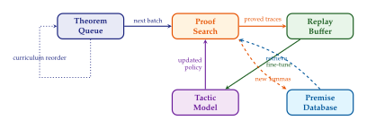
Curriculum Learning Strategy
The curriculum in LeanAgent proceeds through several phases:
Phase 1: Basic tactics. The agent begins with theorems provable in one or two tactics (e.g.,
simp,rfl,exact). These form the foundation of its tactic vocabulary.Phase 2: Library navigation. Theorems requiring the application of specific library lemmas. The agent learns to search the library and identify relevant premises.
Phase 3: Multi-step reasoning. Theorems requiring chains of three to ten tactics, involving case splits, induction, and rewriting.
Phase 4: Advanced proofs. Complex theorems from specialised areas of mathematics (algebra, analysis, topology) that require domain-specific knowledge.
Results and Analysis
LeanAgent demonstrates consistent improvement over its proving lifetime. Over 1,000 episodes, the agent's success rate increases from approximately 30% (the performance of the initial model) to approximately 55%, with the most dramatic gains occurring in phases 2 and 3 of the curriculum.
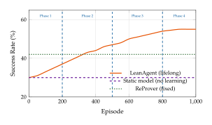
Importantly, LeanAgent does not merely prove more theorems of the same type; it also proves theorems that are qualitatively more difficult than those in its original training set. The dynamic premise database is a key enabler: lemmas proved in early episodes serve as stepping stones for harder theorems in later episodes, mirroring the way human mathematicians build on previously established results.
LeanProgress: Guiding Search via Proof Progress Prediction
A major bottleneck in automated theorem proving is the search problem: the space of possible tactic sequences grows exponentially with proof length, and most branches lead to dead ends. Standard best-first search uses the cumulative log-probability of the tactic sequence as a priority score, but this is a poor proxy for actual progress toward completing the proof. A high-probability tactic may lead to a dead end, while a low-probability tactic may be exactly the creative step needed to break through.
LeanProgress [128] addresses this problem by training a progress predictor: a neural network that, given a proof state, estimates whether the current proof attempt is making progress toward completion.
The Progress Signal
The key insight is that not all proof states are equally promising. Consider two proof states, both resulting from applying a tactic to the same initial goal:
State A: the goal has been simplified, the number of hypotheses has increased (providing more tools), and the remaining goal is a standard library fact.
State B: the goal has become more complex, a new existential quantifier has been introduced, and the hypotheses are unchanged.
Intuitively, State A represents progress while State B represents regression. LeanProgress formalises this intuition by training a classifier on pairs of proof states extracted from successful and unsuccessful proof attempts.
Architecture
The progress predictor takes as input a proof state (encoded as text) and outputs a scalar representing the estimated probability that the current proof attempt will eventually succeed. The model is trained on data from LeanDojo: proof states encountered along successful proof paths are labelled as positive examples, while proof states from failed attempts (that eventually timed out or hit a dead end) are labelled as negative.
During proof search, the progress predictor is used to re-rank the search frontier. Instead of the standard priority score , LeanProgress uses: (Leanprogress Score) where is a mixing coefficient that trades off between the progress estimate and the tactic probability.
Remark 26.
The progress predictor serves a similar role to the value network in AlphaGo [43]: it provides a position evaluation that can guide search beyond what the policy network (tactic generator) alone can achieve. We will explore this connection further in MCTS and Neural Networks: The AlphaZero Paradigm.
Results
LeanProgress improves the success rate of ReProver by approximately 5 percentage points on the LeanDojo Benchmark, with particularly large gains on theorems requiring long proofs (10 or more tactics). For short proofs, the progress predictor provides little benefit (the tactic probability alone is sufficient), but for long proofs, the ability to prune unpromising branches early is critical for staying within the computational budget.
APOLLO: Automated LLM and Lean Collaboration
The systems described so far use a single model for tactic generation. APOLLO [129] takes a different approach: it decomposes the theorem proving task into subtasks handled by specialised agents that collaborate in an iterative refinement cycle.
Multi-Agent Architecture
APOLLO employs three agents:
The Idea Generator: given a theorem statement, this agent produces a high-level proof strategy in natural language (e.g., “proceed by strong induction on , with the base case verified by computation”).
The Prover: given the theorem statement and the proof strategy, this agent generates a complete Lean proof attempt.
The Verifier: submits the proof attempt to the Lean kernel. If the proof fails, the verifier extracts the error messages and the specific tactic that failed, and returns structured feedback to the Idea Generator.
The three agents operate in a loop: the Idea Generator proposes a strategy, the Prover implements it, the Verifier checks it, and if the proof fails, the feedback is used to refine the strategy. This loop continues for a fixed number of iterations or until the proof succeeds.
Iterative Refinement
The iterative refinement cycle is the key to APOLLO's effectiveness. On the first attempt, the proof may fail for various reasons: incorrect lemma application, missing case analysis, or an incorrect induction hypothesis. The error feedback from the Verifier is specific and actionable:
Error at line 7: tactic 'simp' failed
Goal: n + 0 = n
Expected: try 'Nat.add_zero'
Nat.add_zero instead of simp
for the base case”) and the Prover to generate a corrected
attempt.
Empirically, APOLLO's success rate increases significantly with each refinement iteration. On a benchmark of 200 theorems from Mathlib, the first attempt succeeds on approximately 35% of theorems. After three iterations, the success rate rises to 52%. After five iterations, it reaches 58%, with diminishing returns thereafter.
Error Categorisation and Feedback Quality
A critical factor in APOLLO's effectiveness is the quality of the error feedback. Not all error messages from the Lean kernel are equally informative. APOLLO categorises errors into several types:
Type mismatch errors: the tactic produced a term of the wrong type. These are the most informative because they specify exactly what type was expected and what was provided, allowing the Prover to make a targeted correction.
Unknown identifier errors: the tactic references a lemma or definition that does not exist in the current scope. These often indicate that the Idea Generator's strategy referenced a lemma by an incorrect name, and the feedback allows the system to search for the correct name.
Tactic failure errors: the tactic is syntactically valid but does not apply to the current goal (e.g.,
simpfails to simplify because no applicable rewrite rules exist). These are less informative because they do not explain why the tactic failed.Timeout errors: the tactic (or a sub-procedure it invokes) exceeds a time limit. These provide almost no useful information for refinement.
The Verifier agent in APOLLO is specifically designed to extract structured information from error messages and present it to the Idea Generator in a format that facilitates reasoning about the failure. This structured error feedback is one of the key innovations that distinguishes APOLLO from simpler iterative approaches that simply concatenate the raw error message with the original prompt.
TheoremLlama: Transforming LLMs into Lean 4 Experts
The previous systems either use proprietary models (GPT-4) or relatively small models (ByT5) for tactic generation. TheoremLlama [130] explores an alternative approach: fine-tuning a large open-source model (LLaMA [133]) specifically for Lean 4 theorem proving.
Training Data: Synthetic Proof Generation
A central challenge in fine-tuning for theorem proving is the scarcity of training data. While Mathlib contains many theorems, the diversity of proof styles is limited by human conventions. TheoremLlama augments the training data with synthetic proofs generated by the model itself:
Train an initial model on the human-written proofs from Mathlib.
Use the model to generate alternative proofs for theorems in the training set. Some of these alternatives will be valid (verified by the Lean kernel) but stylistically different from the human originals.
Add the verified alternative proofs to the training set.
Repeat the fine-tuning with the augmented dataset.
This self-play-like data augmentation strategy (see Self-Play and Curriculum Learning for a detailed discussion of self-play in the RL context) increases both the volume and diversity of training data.
Fine-Tuning Strategy
TheoremLlama uses a two-stage fine-tuning approach:
Stage 1: Natural language mathematics. The model is fine-tuned on a corpus of natural language mathematical text (textbooks, papers, proofs in English) to strengthen its mathematical reasoning capabilities.
Stage 2: Formal proof code. The model is further fine-tuned on the (augmented) Lean 4 proof corpus, learning to generate syntactically and semantically correct Lean code.
The two-stage approach is motivated by the observation that mathematical reasoning and formal proof writing are related but distinct skills. Stage 1 builds the reasoning foundation; Stage 2 maps that reasoning into the formal language.
Alignment Between Informal and Formal Reasoning
A notable feature of TheoremLlama is its use of aligned pairs during training: for each theorem in the training set, the model is shown both the informal proof (extracted from mathematical textbooks or generated by GPT-4) and the corresponding formal Lean proof. The training objective encourages the model to attend to the informal reasoning when generating formal tactics, creating a bridge between the two modalities.
This alignment has a practical benefit: when a user provides an informal proof sketch (as in Lean Copilot's Mode 3), a model trained with aligned pairs is better at translating the informal reasoning into correct formal tactics. The alignment also improves interpretability: by examining the model's attention patterns, one can identify which parts of the informal reasoning correspond to which formal tactics, providing insight into the model's “thought process.”
Results
TheoremLlama achieves competitive performance with ReProver on the LeanDojo Benchmark while using a fully open-source model. On the random split, it achieves approximately 48% success rate, compared to ReProver's 51%. The gap narrows on the novel premises split (23% vs. 25%), suggesting that the larger model has comparable generalisation ability despite slightly lower overall performance.
Comparative Analysis of Neural Theorem Proving Systems
Table 4 provides a systematic comparison of the neural theorem proving systems discussed in this section.
| System | Base Model | Retrieval | Lifelong | Multi-Agent | Pass Rate |
| ReProver | ByT5 | ✓ | 51.2% | ||
| Lean Copilot | Various | ✓ | - | ||
| LeanAgent | ByT5 | ✓ | ✓ | 55% | |
| LeanProgress | ByT5 | ✓ | 56% | ||
| APOLLO | GPT-4 | ✓ | 58% | ||
| TheoremLlama | LLaMA | 48% |
Several trends emerge from this comparison:
Retrieval is nearly universal. All systems that achieve high performance use some form of premise retrieval. The mathematical library is too large for any model to memorise; explicit retrieval is essential.
Iterative approaches outperform single-shot. Both LeanAgent (which learns over time) and APOLLO (which refines within a single theorem) demonstrate that iteration substantially improves performance.
Open-source models are competitive. TheoremLlama shows that fine-tuned open-source models can approach the performance of systems based on proprietary models, albeit with additional engineering effort.
The field is rapidly evolving. The performance gap between these systems is small (roughly 48–58%), and new systems are being published at an accelerating rate. The numbers in Table 4 should be interpreted as a snapshot of a rapidly moving frontier.
The Neural Theorem Proving Pipeline
Despite their differences, all the systems discussed above share a common pipeline, illustrated in Figure 49. Understanding this pipeline is essential for appreciating both the current state of the art and the directions for future research.
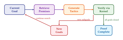
The pipeline has four stages:
Goal extraction: extract the current proof state, including the target proposition (the “goal”) and the available hypotheses and local definitions.
Premise retrieval: search the mathematical library for lemmas, definitions, and theorems that are relevant to the current goal. This step is critical because the library may contain hundreds of thousands of items, and the tactic generator cannot reason about all of them simultaneously.
Tactic generation: use a neural network (typically a Transformer) to generate one or more tactic candidates, conditioned on the goal and the retrieved premises.
Kernel verification: submit each tactic candidate to the proof kernel. If the tactic is valid, it transforms the goal into zero or more new subgoals. If all subgoals are eventually closed, the proof is complete.
Exercises
Exercise 59.
Consider a best-first proof search with branching factor (the number of tactic candidates generated at each step) and maximum depth . (a) What is the worst-case number of nodes explored? (b) How does the retrieval component of ReProver reduce the effective branching factor? (c) Argue that the progress predictor of LeanProgress can be understood as reducing the effective depth by pruning unpromising branches early.
Exercise 60.
Write down the full contrastive loss function used to train the premise retriever in ReProver. Specifically, given a batch of (proof state, premise) pairs , where is a premise actually used in the proof of , define the loss using in-batch negatives (i.e., for each , the premises with serve as negative examples). How does this relate to the InfoNCE loss [44]?
Exercise 61.
Lean Copilot must generate and verify tactic suggestions fast enough for interactive use (target: under 500,ms per suggestion). Suppose the language model generates candidate tactics, each requiring milliseconds to generate and milliseconds to verify. (a) If generation and verification are sequential, what is the total latency to produce the first valid suggestion? (b) If generation is batched (all candidates generated in parallel) and verification is sequential, what is the improved latency? (c) Propose an architecture where verification is also parallelised. What are the resource implications?
Exercise 62.
LeanAgent uses elastic weight consolidation (EWC) to mitigate catastrophic forgetting. Recall that EWC adds a regularisation term to the loss: where are the parameters after training on previous tasks and is the Fisher information for parameter . (a) Explain intuitively why weighting by is better than uniform regularisation. (b) How would you compute in practice for a tactic prediction model? (c) Discuss the limitations of EWC when the number of tasks (episodes) grows very large.
Exercise 63.
In the APOLLO system, the iterative refinement loop converges (the success rate plateaus) after approximately five iterations. (a) What factors limit convergence? Consider the information content of error messages, the diversity of proof strategies, and the base model's capabilities. (b) Propose a modification to the APOLLO architecture that could improve convergence by using a “proof critic” agent that analyses failed attempts and suggests structural changes to the proof strategy.
The Role of Reinforcement Learning in Mathematical Reasoning
In the previous section, we described neural theorem proving systems that generate tactics using supervised learning: a model is trained on human-written proofs to predict the next tactic given a proof state. But supervised learning has a fundamental limitation. It can only learn from existing proofs. If a theorem has never been proved (or if the model needs to discover a proof strategy that no human has used), supervised learning provides no signal.
This is where reinforcement learning (RL) enters the picture. RL allows a model to learn from its own experience: by attempting proofs, observing whether they succeed or fail, and gradually improving its strategy. The marriage of RL and formal theorem proving is particularly natural because the theorem proving task maps cleanly onto the RL framework, and formal verification provides an unusually clean reward signal.
Key Idea.
Formal theorem proving is a near-ideal domain for reinforcement learning because: (1) the state space is well-defined (proof states), (2) the action space is discrete (tactics), (3) the reward is binary and mechanically verifiable (proof accepted or not), and (4) there is no possibility of reward hacking, since the proof kernel is an incorruptible judge.
The Theorem Proving MDP
We begin by formalising theorem proving as a Markov Decision Process (MDP).
Definition 20 (Theorem Proving MDP).
The theorem proving MDP is a tuple where:
is the set of proof states. Each state consists of a set of goals , each with associated hypotheses and a target type (the proposition to be proved). The initial state contains a single goal: the theorem statement.
is the set of actions (tactics). Each tactic is a command that transforms a proof state. Examples include
intro,apply,simp,induction,rw, andexact. The action space is effectively infinite because tactics can take arguments (e.g.,apply Nat.succ_le_succ).is the transition function, determined by the proof kernel. Given a state and a tactic , the kernel either produces a new state or rejects the tactic (in which case we can model the transition as going to the same state with a penalty).
is the reward function. if is a terminal state with no remaining goals (the proof is complete), and otherwise.
is the discount factor. Because proofs have finite length, is typically set to .
Several features of this MDP are worth noting:
Sparse reward.
The reward is extremely sparse. The agent receives only when the proof is complete and for every intermediate step. In a proof requiring 20 tactics, the agent must make 20 correct decisions in sequence before receiving any feedback. This is one of the most challenging reward structures in RL.
Deterministic transitions.
Unlike most RL environments, the transition function is deterministic: given a state and a valid tactic , the resulting state is uniquely determined by the proof kernel. There is no stochasticity in the environment, only in the agent's policy.
Perfect reward signal.
The reward is computed by the proof kernel, which is provably correct (assuming no bugs in the implementation). This means there is no reward hacking, no reward misspecification, and no distributional shift in the reward. The agent either proved the theorem or it did not. This is a luxury that RL researchers in other domains (robotics, game playing, natural language) can only dream of.
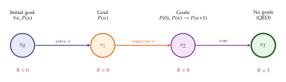
Expert Iteration for Theorem Proving
The simplest RL-inspired approach to theorem proving is Expert Iteration (ExIt) [109], which alternates between two phases: exploration (using the current policy to search for proofs) and training (updating the policy to imitate the successful proofs found during exploration).
The ExIt Algorithm
Definition 21 (Expert Iteration for Theorem Proving).
Given an initial policy (trained by supervised learning on human proofs) and a set of unproved theorems :
Exploration: for each theorem , run proof search using (the current policy) as the tactic generator. Let be the set of successful proof traces.
Training: fine-tune on to obtain . Specifically, minimise the cross-entropy loss: (EXIT LOSS) where the sum is over all (state, tactic) pairs in the successful proofs.
Repeat from step 1 with .
The name “Expert Iteration” comes from the observation that the exploration phase produces an “expert” (the search procedure using ), and the training phase distils the expert's knowledge back into the policy. The expert is better than the raw policy because it uses search (exploring multiple tactic sequences), while the policy is a single forward pass.
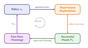
Why ExIt Works
The key insight behind ExIt is that search at inference time is more powerful than the raw policy. Even if assigns low probability to the correct tactic at some step, the search procedure may still find it by exploring many alternatives. The resulting proof trace then provides a training signal that upweights the correct tactic, making the policy better for the next iteration.
Formally, at each iteration, the search-augmented policy (the “expert”) satisfies: (EXIT Improvement) because the expert uses as a component and augments it with search. Training to imitate the expert transfers (some of) this advantage back into the policy, leading to monotonic improvement in expectation.
Practical Considerations
Several practical issues arise when implementing ExIt for theorem proving:
Cold start: the initial policy must be good enough to prove at least some theorems during the first exploration phase. If is too weak, the set of successful proofs will be empty, and no learning occurs. This is why ExIt typically starts from a supervised pre-trained model rather than a random initialisation.
Diminishing returns: in early iterations, the exploration phase discovers many new proofs, but as the policy improves, the marginal gain decreases. The remaining unproved theorems are genuinely harder, and the search budget may be insufficient to find their proofs.
Distribution shift: the training data in later iterations consists of proofs found by earlier policies, which may have idiosyncratic styles. This can lead to mode collapse if not carefully managed (e.g., by always including the original human proofs in the training set).
MCTS and Neural Networks: The AlphaZero Paradigm
Expert Iteration can be significantly strengthened by replacing the simple best-first search with Monte Carlo Tree Search (MCTS), the same search algorithm used by AlphaZero [134] to achieve superhuman performance in Go, chess, and shogi.
MCTS for Proof Search
MCTS explores the proof tree by repeatedly performing four steps: selection, expansion, simulation, and backpropagation. Applied to theorem proving, these steps become:
Selection: starting from the root (the initial proof state), traverse the tree by selecting at each node the action (tactic) that maximises the UCB (Upper Confidence Bound) score: (UCB) where is the average value of taking action in state (estimated from previous simulations), is the policy network's prior probability for action , is the visit count for state , is the visit count for action in state , and is an exploration constant.
Expansion: when a leaf node is reached, expand it by generating tactic candidates using the policy network and verifying each with the proof kernel.
Evaluation: evaluate the leaf node using the value network , which estimates the probability that the proof can be completed from state .
Backpropagation: update the -values and visit counts along the path from the leaf to the root.
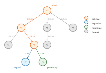
The Policy and Value Networks
The MCTS framework requires two neural networks:
Policy network .
This is the tactic prediction model familiar from the previous section. Given a proof state , it outputs a distribution over tactics. In the MCTS context, the policy provides the prior that biases search toward promising actions.
Value network .
This network estimates the probability that the proof can be completed from state . Training the value network requires labelled data: proof states from completed proofs are labelled , while proof states from failed attempts are labelled . In practice, one can also use the intermediate states from successful proofs as positive examples (with a label equal to the discounted future reward) and states from timed-out searches as negative examples.
The value network serves the same role as LeanProgress's progress predictor (LeanProgress: Guiding Search via Proof Progress Prediction), but is trained within the MCTS framework and used to both evaluate leaf nodes and guide selection.
The AlphaZero Training Loop
The full AlphaZero-style training loop for theorem proving proceeds as follows:
Initialise: train and on human proof data (supervised pre-training).
Self-play: run MCTS-guided proof search on a batch of theorems. For each theorem, record: itemize
The MCTS visit counts at each node (which define an improved policy ).
The outcome (whether the proof was found). itemize
Train: update the policy network to match the MCTS visit counts and the value network to predict the outcome: (Alphazero LOSS)
Repeat from step 2 with the updated networks.
Remark 27.
A critical difference between AlphaZero for games and AlphaZero for proofs is the reward structure. In games, the outcome is always determined (win/loss/draw) after a finite number of moves. In theorem proving, many proof attempts time out without reaching a definitive conclusion. The treatment of these timed-out episodes (as failures? as partial successes?) is an important design choice that significantly affects training.
Computational Complexity of MCTS for Proofs
The computational cost of MCTS is dominated by two factors: the number of simulations per move and the cost of each simulation. In game playing, each simulation involves running the game to completion using a fast rollout policy. In theorem proving, the analogous operation would be running a complete proof search from each leaf node, which is prohibitively expensive. This is why the value network is essential: it provides an instantaneous estimate of the leaf value, replacing the need for full rollouts.
The total computation per proof attempt is approximately: (MCTS COST) where is the proof depth, is the number of MCTS simulations per step, is the cost of a policy network forward pass, is the cost of a value network forward pass, and is the cost of verifying a tactic with the proof kernel. In practice, is often the dominant term, as invoking the Lean kernel for each tactic involves compilation and type-checking overhead.
Typical configurations use and set a timeout of 10 to 60 minutes per theorem. The computational budget is a significant practical constraint, and much of the engineering effort in neural theorem proving goes into optimising the interaction with the proof kernel to reduce .
PPO vs GRPO for Mathematical Reasoning
While MCTS-based approaches dominate for tree-structured proof search, many recent systems use policy gradient methods to optimise the tactic generation model directly. Two prominent approaches are Proximal Policy Optimisation (PPO) [115] and Group Relative Policy Optimisation (GRPO) [51].
PPO for Theorem Proving
PPO optimises the policy by maximising a clipped surrogate objective: (PPO Objective) where is the probability ratio between the new and old policies, and is the estimated advantage function.
The advantage is typically estimated using Generalised Advantage Estimation (GAE) [135]: (GAE) where is the TD residual and is a learned value function.
The value function problem.
PPO requires a learned value function to estimate the advantage. In theorem proving, this value function is difficult to learn accurately because:
The reward is sparse: for almost all states, making the function nearly constant and uninformative.
Proof states are highly structured text objects, and small changes in the proof state (e.g., changing a single hypothesis) can dramatically change the value.
The value function introduces approximation error, which propagates through the advantage estimate and can destabilise training.
GRPO for Theorem Proving
Group Relative Policy Optimisation (GRPO) [51] avoids the need for a learned value function by estimating the advantage directly from groups of sampled outcomes.
The GRPO procedure for a single theorem is:
Sample complete proof attempts from the current policy . Each attempt is a sequence of tactics that either succeeds (reward ) or fails (reward ).
Compute the group-relative advantage for each attempt: (GRPO Advantage) where is the group mean reward and is its standard deviation.
Update the policy using the clipped objective (same as PPO, but with the GRPO advantage): (GRPO Objective)
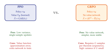
Detailed Comparison
Figure 53 summarises the key differences between PPO and GRPO. We elaborate on several points:
Stability.
GRPO is generally more stable for mathematical reasoning because it avoids the compounding errors of a learned value function. In theorem proving, where the reward is binary and sparse, the value function is particularly difficult to learn accurately. GRPO sidesteps this issue entirely by using the empirical group statistics as a baseline.
Sample efficiency.
PPO is more sample-efficient per theorem because it can learn from a single trajectory using the value function as a baseline. GRPO requires samples per theorem (typically to ) to compute meaningful group statistics. For theorems where the success rate is very low, most of the samples will fail, providing limited signal.
Scalability.
GRPO scales better to large models because it avoids the need to train and maintain a separate value network (which, for large language models, can be nearly as expensive as the policy itself). This is a significant practical advantage, as modern theorem proving systems often use models with billions of parameters.
Empirical results.
On mathematical reasoning benchmarks (including GSM8K, MATH, and formal theorem proving), GRPO-trained models consistently match or slightly outperform PPO-trained models, with the advantage being most pronounced on problems with sparse rewards [51].
Reward Shaping for Theorem Proving
The sparse reward problem in theorem proving is severe: the agent receives only upon completing a proof, which may require dozens of correct tactic applications in sequence. Reward shaping introduces intermediate rewards that guide the agent toward the terminal reward without changing the optimal policy.
Potential-Based Reward Shaping
The classical theory of reward shaping [136] shows that adding a potential-based shaping reward preserves the optimal policy. Specifically, if is a potential function, then the shaped reward: (PBRS) yields the same optimal policy as the original reward .
For theorem proving, natural choices for include:
Number of remaining goals: . This rewards tactics that close goals and penalises tactics that create new subgoals. However, it can be misleading: some productive tactics (e.g.,
cases) increase the number of goals while bringing the proof closer to completion.Complexity of goal expressions: is the negative of the total size (number of AST nodes) of all goal expressions. This rewards simplification and penalises elaboration.
Value network estimate: , the learned value network. This is the most sophisticated option and can capture subtle notions of progress that hand-crafted potentials miss.
Proof progress predictor: , using the LeanProgress-style predictor. This provides a data-driven estimate of how “close” the proof state is to completion.
Intermediate Reward Signals
Beyond potential-based shaping, several heuristic reward signals have been proposed:
Goal reduction reward.
Award each time a tactic reduces the number of open goals. This is not potential-based (it can change the optimal policy in theory) but works well in practice because goal reduction is almost always a sign of progress.
Successful tactic reward.
Award each time a tactic is accepted by the kernel (as opposed to being rejected). This provides a weak but ubiquitous signal that encourages syntactically and semantically valid tactics.
Novelty reward.
Award a small bonus for reaching proof states that have not been visited before (analogous to curiosity-driven exploration [137]). This encourages the agent to explore diverse proof strategies rather than repeatedly trying the same failing approach.
Hindsight Experience Replay
A particularly elegant approach to the sparse reward problem is Hindsight Experience Replay (HER) [138], adapted to the theorem proving setting.
The idea is simple: when a proof attempt fails (the agent does not prove the intended theorem), examine what the agent did prove. In many cases, the agent's tactic sequence, while not closing the original goal, does establish some intermediate result. This intermediate result can be extracted as a “proved lemma” and the failed trajectory can be relabelled as a successful proof of this lemma.
Definition 22 (Hindsight Experience Replay for Proofs).
Given a failed proof attempt for theorem , where has remaining goals :
Identify the hypotheses in that were not present in . These represent intermediate results established by the agent's tactics.
Construct a “hindsight theorem” whose statement is one of these intermediate results.
Relabel the trajectory as a successful proof of and add it to the training buffer.
HER provides a rich source of training signal from failed proof attempts, which constitute the vast majority of the agent's experience. It also naturally creates a curriculum of lemmas of increasing difficulty, as the agent's improving policy produces increasingly sophisticated intermediate results.
Example 44.
HER in action.
Suppose the agent attempts to prove
.
The agent successfully applies intro n,
induction n, and closes the base case, but fails on
the inductive step. The final proof state has an established
hypothesis .
HER extracts this as a “hindsight theorem”: the base case of
the summation identity. The trajectory is relabelled as a
successful proof of ,
providing a positive training signal from what was originally
a failure.
Combining Reward Shaping Strategies
In practice, the most effective systems combine multiple reward shaping strategies. A typical configuration uses:
A potential-based shaping reward with (the learned value network) as the primary signal.
A small bonus () for each valid tactic application to encourage syntactically correct output.
Hindsight experience replay to extract training signal from failed attempts.
The combination addresses different aspects of the sparse reward problem: the potential-based shaping provides a smooth gradient toward proof completion, the validity bonus encourages basic competence, and HER ensures that no computation is wasted.
Self-Play and Curriculum Learning
A limitation of all the approaches discussed so far is that they operate on a fixed set of theorems. The agent can prove more theorems from this set over time, but it cannot generate new mathematical content. Self-play addresses this limitation by allowing the agent to generate its own conjectures, attempt to prove them, and learn from the experience.
Conjecture Generation
The self-play cycle for theorem proving involves two roles:
The Conjecturer: generates new theorem statements (conjectures) in the formal language. Not all generated statements are valid theorems; some may be false, trivially true, or syntactically ill-formed.
The Prover: attempts to prove the generated conjectures. A conjecture that is proved becomes a new lemma that can be used in future proofs. A conjecture that resists all proof attempts may be false or simply too hard.
The Conjecturer and Prover can be the same model (with different prompts) or separate models. The key insight is that the Conjecturer should generate theorems that are at the boundary of the Prover's ability: easy enough that some can be proved (providing positive training signal) but hard enough that the Prover must improve to prove them (providing learning pressure).
Curriculum via Self-Play
Self-play naturally creates a curriculum. In early iterations, when the Prover is weak, the Conjecturer generates simple theorems (because its own mathematical knowledge is limited). As both models improve, the conjectures become more sophisticated and the proofs more complex. This co-evolution between the Conjecturer and the Prover mirrors the way mathematical knowledge develops in the human mathematical community: new results build on previous ones, and the frontier of knowledge advances incrementally.
Proposition 3 (Self-Play Improvement).
Let and denote the Prover and Conjecturer policies at iteration , respectively. If the Conjecturer generates theorems at the boundary of the Prover's ability (i.e., the Prover succeeds on approximately 50% of generated conjectures), then the expected improvement in the Prover's success rate per iteration is maximised.
Proof.
The training signal for the Prover comes from both successful and failed proof attempts. If the success rate is too high (close to 100%), most conjectures are trivial and provide no learning pressure. If the success rate is too low (close to 0%), the sparse reward problem becomes extreme and the Prover receives almost no positive signal. The information-theoretic optimum is at 50%, where each conjecture provides one bit of information about the Prover's boundary of competence. This is the standard argument for optimal curriculum difficulty from the educational psychology literature [45], adapted to the self-play setting.
Practical Implementation
Implementing self-play for theorem proving requires several engineering decisions:
Filtering conjectures: not all generated statements are worth attempting to prove. Trivially true statements (e.g., ) should be filtered out. Syntactically ill-formed statements should be rejected. False statements can be detected (heuristically) by attempting to find counterexamples.
Difficulty estimation: to maintain the optimal curriculum, the Conjecturer must estimate the difficulty of generated conjectures. This can be done by having the Prover make a quick attempt (with a small budget) and using the outcome to calibrate difficulty.
Novelty: the Conjecturer should be encouraged to generate diverse conjectures rather than variations of the same theorem. Diversity can be promoted through entropy regularisation, rejection of duplicates, or by conditioning the Conjecturer on different mathematical topics.
Remark 28.
The self-play approach to theorem proving has a provocative implication. If the system generates and proves conjectures that are genuinely new (not found in any existing library), it is performing mathematical discovery. Whether such machine-generated mathematics is “interesting” or “meaningful” is a philosophical question that we will not attempt to settle here, but the potential is clear.
Connections to Open-Ended Evolution
The self-play loop for theorem proving bears a striking resemblance to the open-ended evolutionary processes discussed in the chapter on Evolutionary AI. In both cases, the system generates its own “problems” (mutations in evolutionary search, conjectures in theorem proving) and its own “solutions” (phenotypes, proofs). The resulting dynamics can exhibit the hallmarks of open-ended evolution: increasing complexity, innovation, and the emergence of structures that were not explicitly programmed.
This connection suggests that ideas from artificial life and open-ended search (quality-diversity optimisation, novelty search, minimal criterion coevolution) may be productively applied to the mathematical reasoning domain. For example, instead of optimising purely for the number of theorems proved, one could maintain a diverse archive of proof strategies (as in MAP-Elites) and reward the discovery of qualitatively new proof techniques rather than incremental extensions of known methods.
Summary: The RL Landscape for Mathematical Reasoning
We conclude this section by summarising the key RL approaches to mathematical reasoning and their relationships.
| Approach | Reward | Search | Value Network | Key Advantage |
| ExIt | Sparse (0/1) | Best-first | No | Simplicity |
| MCTS + NN | Sparse (0/1) | MCTS | Yes | Strong search |
| PPO | Shaped | None | Yes | Sample efficiency |
| GRPO | Sparse (0/1) | None | No | Stability |
| Self-play | Sparse (0/1) | Various | Optional | Data generation |
Table 5 highlights the design space. The choice of RL method depends on several factors:
If computational resources are limited, ExIt provides a simple and effective baseline.
If one can afford the computational cost of MCTS, the AlphaZero paradigm provides the strongest search.
If training stability is a concern, GRPO is preferable to PPO for mathematical reasoning.
If the goal is to discover new mathematics (not just prove existing theorems), self-play is the most natural framework.
The field is converging on a synthesis of these approaches: a system that uses GRPO or PPO to train a policy network, MCTS for proof search at inference time, and self-play to generate a curriculum of training problems. Whether such a system can achieve “superhuman” mathematical reasoning, proving theorems that no human has proved, remains one of the most exciting open questions in AI.
Exercises
Exercise 64.
Consider the following Lean 4 theorem:
theorem add_comm (n m : Nat) : n + m = m + n
Nat.add_comm. Be explicit about the proof state at
each step, including all goals and hypotheses. What is the
total (undiscounted) return for this trajectory?Exercise 65.
In Expert Iteration, the policy improves monotonically in the sense that the search-augmented expert at iteration is at least as good as the expert at iteration . (a) Formalise this claim. Under what assumptions does it hold? (b) Does the raw policy (without search) also improve monotonically? Give a counterexample or a proof. (c) Under what conditions does ExIt converge to the optimal policy (one that proves every provable theorem)?
Exercise 66.
The exploration constant in the UCB formula ((UCB)) trades off between exploitation (following the current best estimates) and exploration (trying under-visited actions). (a) What happens when ? When ? (b) In AlphaGo, is a fixed hyperparameter. Propose an adaptive scheme for choosing in the theorem proving setting, where different proof states may require different levels of exploration. (c) How does the policy prior interact with the exploration constant? Can a very good policy compensate for a poorly chosen ?
Exercise 67.
Consider a theorem where the Prover's success rate is (i.e., 5% of proof attempts succeed). Suppose we use GRPO with group size . (a) Compute the expected value of and as a function of and . (b) What is the probability that all samples fail (in which case and , providing no training signal)? (c) How large must be to ensure that at least one sample succeeds with probability ? (d) Compare this to the sample requirement for PPO with a learned value function. Under what conditions is GRPO more sample-efficient despite requiring multiple samples per theorem?
Exercise 68.
Prove that potential-based reward shaping ((PBRS)) preserves the optimal policy. Specifically, show that if is optimal under reward , then is also optimal under the shaped reward . Hint: show that the shaped and unshaped value functions differ by the potential function, i.e., for all policies and states .
Exercise 69.
Implement (in pseudocode) Hindsight Experience Replay for theorem proving. Your pseudocode should:
Take as input a failed proof trajectory and the original theorem statement.
Extract the intermediate results (new hypotheses) from the final proof state.
Construct a “hindsight theorem” whose proof is the prefix of the original trajectory.
Return the relabelled trajectory.
Discuss the potential pitfalls: what if the intermediate result is trivial? What if it is actually false (due to a bug in the extraction)? How would you filter out low-quality hindsight theorems?
Exercise 70.
Design a scoring function for evaluating the quality of machine-generated conjectures. Your scoring function should penalise: (a) trivially true statements, (b) syntactically ill-formed statements, (c) statements that are isomorphic to existing theorems in the library (up to variable renaming), and (d) statements that are “uninteresting” (however you choose to define this). Discuss how each component of your scoring function could be implemented in practice. Is there a fundamental tension between (c) and (d)?
Exercise 71.
Write complete pseudocode for a PPO-based theorem proving system. Your pseudocode should cover:
Initialisation of the policy and value networks.
The rollout phase (generating proof attempts).
Computing the GAE advantage estimates.
The policy update (with clipping).
The value function update.
Be explicit about how you handle: (a) variable-length proof trajectories, (b) the sparse reward structure, and (c) the interaction with the proof kernel for trajectory generation.
AlphaProof: DeepMind's IMO Solver
On July 17, 2024, six hundred of the world's most gifted young mathematicians sat down in Bath, England, to face six problems at the 65th International Mathematical Olympiad (IMO). They had four and a half hours for the first three problems on Day 1, and another four and a half hours for the remaining three on Day 2. Each problem was worth seven points, for a maximum score of 42. The gold medal threshold that year was 29 points. The silver medal threshold was 22 points.
What the contestants did not know was that, in a server room on the other side of the world, an AI system developed by Google DeepMind was simultaneously attempting the same six problems. The system consisted of two complementary components: AlphaProof, a reinforcement-learning-based theorem prover built on the Lean formal language, and AlphaGeometry 2, a neuro-symbolic system specialised for Euclidean geometry. Together, they solved four of the six problems, earning 28 out of 42 points, a performance equivalent to a silver medal and just one point short of gold [46].
Key Idea.
AlphaProof represents the culmination of a research lineage that began with AlphaGo in 2016: the idea that Monte Carlo tree search (MCTS) combined with learned neural network evaluations and reinforcement learning from self-play can master domains where brute-force search is intractable. In AlphaProof, the “game” is theorem proving, the “moves” are Lean tactics, and “winning” means closing all proof goals.
The Story of IMO 2024
The International Mathematical Olympiad is widely regarded as the most prestigious mathematics competition in the world. Since its founding in 1959, it has served as a proving ground for mathematical talent: Fields Medallists Terence Tao, Grigori Perelman, and Maryam Mirzakhani all competed as teenagers. The problems span combinatorics, algebra, geometry, and number theory, and are designed to require deep insight rather than rote calculation. A perfect score is exceedingly rare; in most years, fewer than five contestants achieve it.
The 2024 competition featured problems ranging from elementary (by Olympiad standards) to exceptionally hard. Problem 1 asked about a combinatorial property of real numbers. Problem 2 involved functional equations in algebra. Problem 3 was a geometry problem about cyclic quadrilaterals. Problem 4 concerned algebraic inequalities. Problem 5 was a combinatorial problem about sequences. Problem 6, traditionally the hardest position on the paper, asked about a combinatorial game involving turbo the snail traversing a grid, and only five human contestants solved it perfectly.
DeepMind's entry was not a single monolithic system but a collaboration between two architecturally distinct approaches [46]:
AlphaProof: a general-purpose theorem prover that combines a fine-tuned Gemini language model (for translating natural-language problem statements into formal Lean specifications) with an AlphaZero-style reinforcement learning agent (for searching over Lean proof tactics). AlphaProof attacked all six problems.
AlphaGeometry 2: an improved version of the neuro-symbolic geometry solver AlphaGeometry, which combines a neural language model trained on synthetic geometry data with a symbolic deduction engine. AlphaGeometry 2 was deployed specifically for the geometry problem (Problem 3) and also contributed to Problem 5 after the problem was reformulated in geometric terms.
The results were striking. AlphaProof solved Problems 1, 2, and 6, earning full marks on each (21 out of 21 points). AlphaGeometry 2 solved Problem 5, earning an additional 7 points. Problems 3 and 4 remained unsolved. The total of 28 points placed the AI system above the silver medal threshold of 22 and just below the gold medal threshold of 29.
Remark 29.
The timing constraints differed dramatically between humans and the AI system. Human contestants had approximately 4.5 hours per set of three problems. AlphaProof, by contrast, was given up to three days of compute per problem, running on a large cluster of TPUs. Problem 6, the hardest, required roughly 72 hours of search. This asymmetry is important: AlphaProof's achievement is remarkable, but it is not yet an “apples-to-apples” comparison with human performance.
The AlphaGo to AlphaProof Lineage
AlphaProof did not emerge from a vacuum. It is the latest in a sequence of systems that began with DeepMind's work on the game of Go and progressively generalised the core ideas to broader domains. Understanding this lineage is essential for appreciating both the design of AlphaProof and its limitations.
AlphaGo (2016): Neural Networks Meet Monte Carlo Tree Search
In March 2016, AlphaGo defeated Lee Sedol, one of the strongest Go players in history, by four games to one [43]. The result stunned the AI community. Go had long been considered a grand challenge for artificial intelligence: its branching factor (approximately 250 legal moves per position, compared to roughly 35 in chess) made traditional game-tree search intractable, and its positional evaluation seemed to require a form of intuition that resisted codification.
AlphaGo combined four key ideas:
Policy network : a deep convolutional neural network trained on millions of human Go games to predict the probability that a strong human player would play move in position . This network reduced the effective branching factor from 250 to a manageable handful of candidate moves.
Value network : a second deep convolutional neural network trained to predict the probability of winning from position . This network replaced the need for full rollouts to the end of the game.
Monte Carlo tree search (MCTS): a search algorithm that builds a partial game tree by repeatedly simulating games. At each simulation step, MCTS selects moves using the upper confidence bound for trees (UCT) formula, which balances exploitation (moves that look good) with exploration (moves that have not been tried often): (UCT) where is the average value of simulations passing through action from state , is the visit count of state , is the visit count of action from , and is an exploration constant.
Reinforcement learning from self-play: after the initial training on human games, AlphaGo was further improved by playing millions of games against itself, using the outcomes to update both the policy and value networks.
AlphaZero (2017): Tabula Rasa Learning
In 2017, DeepMind introduced AlphaZero, which achieved superhuman performance in Go, chess, and shogi (Japanese chess) starting from no human knowledge whatsoever, not even the rules of the game beyond the basic mechanics of legal moves and outcomes [134]. AlphaZero simplified and unified the AlphaGo architecture:
A single neural network that takes a board state as input and simultaneously outputs a policy vector (a probability distribution over moves) and a scalar value (the estimated probability of winning).
Pure MCTS guided by this network, with no rollouts and no handcrafted heuristics.
Training entirely from self-play: the network is initialised with random weights, plays millions of games against itself, and is trained to predict the MCTS-improved policy and the eventual game outcome.
The training loop is elegantly simple. In each iteration:
The current network plays games against itself, using MCTS to select moves. For each position encountered during play, record the MCTS visit counts (a vector of probabilities derived from how often each move was explored) and the final game outcome .
Train on the collected data by minimising a loss that combines policy accuracy and value accuracy: (Alphazero LOSS) where and are the value and policy outputs of the network, and is a regularisation coefficient.
Replace the current network with the newly trained one and repeat.
The key insight is that MCTS acts as a policy improvement operator: the search process, guided by the current network, produces a policy that is strictly better than the raw network policy . By training the network to match , one obtains a better network, which in turn produces a better MCTS policy, creating a virtuous cycle of improvement.
Key Idea.
The AlphaZero paradigm can be summarised as: neural network provides fast, approximate evaluation; tree search provides slow, accurate evaluation; training closes the gap between the two. This paradigm is domain-independent: it works for any sequential decision problem where states are observable and outcomes are verifiable.
From Games to Proofs: The Key Insight
The leap from AlphaZero to AlphaProof rests on a single powerful observation: formal theorem proving is structurally identical to a single-player game.
Definition 23 (Theorem Proving as a Game).
A formal theorem proving problem can be cast as a single-player game with the following components:
State: the current proof state in Lean, consisting of a list of open goals (propositions that remain to be proved), together with the local context (hypotheses and definitions in scope).
Actions: the set of Lean tactics applicable to the current proof state (e.g.,
intro,apply,rw,simp,ring,omega,exact, etc.).Transitions: applying a tactic to a proof state produces a new proof state (possibly with fewer open goals, or with the current goal replaced by subgoals).
Terminal condition: the proof is complete when no open goals remain. The proof “wins” if the original theorem statement has been established.
Reward: if the proof is completed successfully; or otherwise.
This analogy, while conceptually clean, involves several important differences from board games:
Variable branching factor. In Go, the branching factor is roughly constant at 250. In theorem proving, the number of applicable tactics varies enormously: some proof states admit only a handful of meaningful tactics, while others (especially those involving existential witnesses or complicated rewrite sequences) may admit thousands.
Unbounded episode length. A Go game lasts at most moves. A proof can, in principle, be arbitrarily long, and the depth of the search tree is not bounded a priori.
Sparse and delayed rewards. In Go, the outcome (win/loss) is known after at most 361 moves. In theorem proving, the agent may explore hundreds of tactic applications before reaching either a completed proof or a dead end.
Asymmetric verification. In Go, determining whether a position is legal requires only checking the rules. In theorem proving, Lean's type checker provides perfect verification: if Lean accepts the proof, it is correct, with mathematical certainty. This is a significant advantage over board games, where evaluation is inherently approximate.
No opponent. Theorem proving is a single-player game, which means the minimax structure of two-player games is absent. However, one can view the “opponent” as the difficulty of the theorem itself.
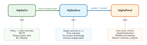
How AlphaProof Works in Detail
We now describe the AlphaProof system in detail, following the pipeline from problem statement to completed proof [46].
Stage 1: Autoformalization
The first stage translates a natural-language mathematical problem statement into a formal theorem statement in Lean 4. This is a non-trivial task: natural-language mathematics is ambiguous, relies on implicit conventions, and uses notation that is often context-dependent. Formal Lean statements, by contrast, must be completely precise and type-correct.
Example 45.
Consider a simplified competition problem: “Prove that for all positive integers , the sum equals .” A corresponding Lean 4 formalization might be:
theorem sum_first_n (n : Nat) (hn : 0 < n) :
Finset.sum (Finset.range (n + 1)) id
= n * (n + 1) / 2 := by
sorry
sorry tactic is a placeholder indicating that the
proof is not yet provided. The goal of AlphaProof is to replace
sorry with a valid proof.AlphaProof uses a fine-tuned version of Google's Gemini language model for autoformalization. The model was trained on a large corpus of paired examples: natural-language mathematical statements alongside their formal Lean counterparts, drawn from Mathlib (the community-maintained library of formalised mathematics in Lean) and from manually curated competition problem sets [46].
The formalization stage is critical and error-prone. If the formal statement does not faithfully capture the intended mathematical content, then even a correct proof of the formal statement may not constitute a solution to the original problem. To mitigate this risk, AlphaProof generates multiple candidate formalizations and uses heuristic checks (e.g., type-checking in Lean, checking that the statement is not trivially true or false) to filter candidates. Human experts also reviewed the formalizations for the IMO problems.
Stage 2: Pre-training on Mathlib
Before tackling competition problems, the AlphaProof agent is pre-trained on a large corpus of existing formal proofs. The primary source is Mathlib, which (as of 2024) contains over 180,000 formalised theorems spanning algebra, analysis, topology, number theory, and combinatorics.
The pre-training objective is analogous to the supervised learning phase in AlphaGo: the policy network is trained to predict the next tactic given the current proof state, using human-written proofs as training data. The value network is trained to predict whether a given proof state will eventually lead to a completed proof.
Formally, let denote the pre-training dataset, where each trajectory corresponds to a completed proof. The pre-training loss is: (Alphaproof Pretrain) where is the policy network, is the value network, and is a coefficient balancing the two objectives. The value target is for all states on a successful proof trajectory (since they all eventually lead to a completed proof).
Stage 3: Reinforcement Learning from Self-Play
After pre-training, AlphaProof enters a reinforcement learning loop that is the direct descendant of AlphaZero's self-play training. The key difference is that “self-play” in the theorem proving context means the agent attempts to prove theorems of increasing difficulty, with successful proofs providing positive reward signals.
The training loop proceeds as follows:
Theorem selection. Select a batch of theorem statements from a curriculum of increasing difficulty. The curriculum includes: (a) theorems from Mathlib whose proofs have been withheld; (b) variations of known theorems generated by perturbation (changing constants, generalising conditions); and (c) competition-style problems from a curated dataset [46].
Proof search via MCTS. For each theorem, run AlphaZero-style MCTS over the space of Lean tactics. At each node of the search tree (corresponding to a proof state ), the neural network provides a policy (a distribution over candidate tactics) and a value (the estimated probability of eventually completing the proof). MCTS selects tactics using the PUCT formula: (PUCT) where is the mean value of all simulations passing through action , is the visit count, and is an exploration constant.
Lean verification. Each tactic application is verified by the Lean type checker. If the tactic produces an error (type mismatch, tactic failure, timeout), the corresponding branch of the search tree is pruned. If all goals are closed, the proof is complete and verified.
Training update. Successful proofs are added to the training buffer. The policy and value networks are updated using a loss analogous to (Alphazero LOSS): (Alphaproof RL LOSS) where is the replay buffer, is the MCTS-improved policy (derived from visit counts), and is the proof outcome.
Iterate. Return to step 1 with the updated network. As the network improves, the curriculum difficulty increases, providing a steady supply of challenging but tractable training problems.
Remark 30.
A crucial difference between AlphaProof's self-play and AlphaZero's self-play is the source of training signal. In AlphaZero, the agent plays against itself, and the outcome of each game provides a clear win/loss signal. In AlphaProof, there is no opponent; the agent attempts to prove theorems, and the signal comes from whether the proof is completed. This means the agent must have a supply of theorems of appropriate difficulty: too easy and the signal is trivial; too hard and the signal is too sparse. The curriculum design is therefore a critical engineering challenge.
Stage 4: Test-Time Compute
At inference time, when confronted with a new problem (such as an IMO question), AlphaProof invests massive computational resources in the search process. Unlike a language model that generates a response in a single forward pass, AlphaProof runs MCTS for extended periods, potentially exploring millions of proof states.
For the IMO 2024 problems, AlphaProof was given up to three days of compute per problem, running on a cluster of Google's TPU accelerators. The search explored vast proof trees, sometimes reaching depths of hundreds of tactic applications. Problem 6 (the combinatorial game problem about turbo the snail), which only five human contestants solved perfectly, required approximately 72 hours of continuous search.
The test-time compute scaling is a distinctive feature of the AlphaProof approach. While language models exhibit diminishing returns from additional inference-time compute (beyond a certain point, generating more tokens or sampling more completions does not help), tree search methods like MCTS can continue to improve with additional compute, as deeper and wider search discovers proofs that shallower search misses.
(Testtime Scaling) where is the compute budget (measured in MCTS simulations) and is a difficulty-dependent scale parameter. This exponential scaling law suggests that, for problems of bounded difficulty, success probability approaches 1 as compute increases, but harder problems require exponentially more compute.
This scaling behaviour has profound implications for the economics of AI-driven mathematics. If a problem can be solved with MCTS simulations, then doubling the compute budget from to increases the success probability from approximately to . But if the problem is ten times harder (), achieving the same success probability requires simulations. The implication is that test-time compute scaling is highly effective for problems within a certain difficulty range, but the range shifts dramatically with the quality of the underlying policy and value networks.
Remark 31.
The test-time compute paradigm represents a fundamentally different philosophy from the “scaling laws” that have dominated LLM research, which focus on increasing model size and training data. AlphaProof's approach suggests that, at least for mathematical reasoning, the returns from test-time compute (deeper search) may exceed the returns from training-time compute (larger models) beyond a certain threshold. This observation has influenced the broader AI research community, contributing to increased interest in inference-time scaling methods across domains.
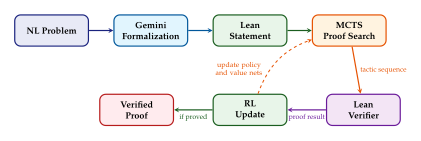
AlphaGeometry and AlphaGeometry 2
While AlphaProof represents a general-purpose approach to theorem proving (in principle applicable to any domain formalisable in Lean), DeepMind also developed a complementary system specialised for Euclidean geometry: AlphaGeometry, and its successor AlphaGeometry 2 [47].
The motivation for a specialised geometry solver is twofold. First, geometry problems have a distinctive structure: they involve diagrams, constructions, and spatial relationships that are not naturally expressed in the tactic-based framework of Lean. Second, the space of useful “moves” in geometry proofs is qualitatively different from those in algebraic or combinatorial proofs: the key challenge is often to find the right auxiliary construction (an additional point, line, or circle that, once introduced, makes the proof straightforward).
The AlphaGeometry Architecture
AlphaGeometry uses a neuro-symbolic architecture with two complementary components:
Symbolic deduction engine (DD+AR). The deductive database with algebraic reasoning (DD+AR) is a deterministic engine that, given a set of geometric premises (points, lines, circles, and their relationships), exhaustively applies deduction rules (angle chasing, similar triangles, power of a point, etc.) to derive all consequences [47]. The DD+AR engine is complete for a large fragment of Euclidean geometry: if a theorem can be proved using the available rules, DD+AR will find the proof, provided the right auxiliary constructions have been added to the diagram.
Neural language model. A transformer-based language model, trained on millions of synthetic geometry problems, that suggests auxiliary constructions. When DD+AR cannot complete a proof directly, the language model proposes new geometric objects (e.g., “let be the midpoint of ”, “let be the circumcircle of ”) that may enable DD+AR to close the proof.
The interaction between the two components follows an iterative protocol:
Parse the problem statement and extract the geometric premises and the goal.
Run DD+AR on the current set of premises.
If DD+AR proves the goal, return the proof.
If DD+AR fails, feed the current proof state (premises, derived facts, and the remaining goal) to the neural language model.
The language model generates a ranked list of candidate auxiliary constructions.
Add the top-ranked construction to the premises and return to step 2.
Repeat until the proof is found or a maximum number of iterations is reached.
Key Idea.
AlphaGeometry embodies a clean division of labour: the neural model provides intuition (suggesting which auxiliary constructions might be useful), while the symbolic engine provides rigour (verifying that the proof is logically valid). This neuro-symbolic design avoids the hallucination problem that plagues purely neural approaches to mathematics.
Synthetic Data Generation for Geometry
A distinctive feature of AlphaGeometry is its training data strategy. Rather than relying on the relatively small corpus of existing geometry problems (there are only a few thousand competition geometry problems in existence), the system generates its own training data through a synthetic theorem generation process:
Sample a random set of geometric objects (points, lines, circles) and a random set of constraints (collinearity, concyclicity, parallelism, etc.).
Run DD+AR forward to derive all consequences of these constraints.
Select a non-trivial derived fact as the “theorem” and the initial constraints as the “premises.”
If the proof requires auxiliary constructions (i.e., if intermediate objects were introduced during the derivation that are not among the initial premises), record these constructions as the training target for the neural model.
This process generated over 100 million synthetic geometry problems with associated proofs. Critically, the synthetic data includes the auxiliary constructions needed for each proof, providing direct supervision for the neural language model.
The quality of the synthetic data is ensured by the soundness of the DD+AR engine: every derived fact is a genuine theorem of Euclidean geometry, and every recorded proof is a valid logical derivation. This contrasts sharply with the situation for natural-language mathematics, where synthetic data may contain errors or hallucinations. The synthetic generation process also naturally controls for difficulty: theorems that require more auxiliary constructions are “harder” and provide more informative training signals.
A remarkable finding was that the synthetic data, despite being generated by a relatively simple random process, covers a surprisingly large fraction of the proof techniques used in actual competition geometry. An analysis by the AlphaGeometry team found that approximately 80% of IMO geometry problems from the past decade could, in principle, be proved using the reasoning patterns present in the synthetic training set [47]. The remaining 20% require proof techniques (such as inversive geometry or projective methods) that fall outside the scope of the DD+AR engine.
AlphaGeometry 2: Improvements and IMO 2024
AlphaGeometry 2 introduced several improvements over the original system [46]:
A more powerful neural language model based on the Gemini architecture, trained on a larger synthetic dataset.
An expanded set of deduction rules in the DD+AR engine, covering a broader fragment of Euclidean geometry.
Better integration with the AlphaProof pipeline, allowing geometry problems to be formalized in Lean and attacked by both systems.
A search procedure that explores multiple auxiliary construction sequences in parallel, rather than committing greedily to the top-ranked construction.
On a benchmark of 30 historical IMO geometry problems, AlphaGeometry 1 solved 25. AlphaGeometry 2 solved 28, approaching the performance of the strongest human competitors.
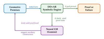
The Relationship Between AlphaProof and AlphaGeometry
AlphaProof and AlphaGeometry represent two fundamentally different philosophies for AI-driven theorem proving, and their complementarity was essential to DeepMind's success at IMO 2024.
| Aspect | AlphaProof | AlphaGeometry |
| Scope | General-purpose | Geometry only |
| Formal language | Lean 4 | Custom symbolic |
| Search method | MCTS (AlphaZero-style) | Iterative construction |
| Verification | Lean type checker | DD+AR engine |
| Training paradigm | RL from self-play | Supervised on synthetic data |
| Key strength | Generality, rigour | Domain-specific insight |
| Key weakness | Compute-intensive | Limited to geometry |
| Training data | Mathlib + competitions | 100M+ synthetic problems |
The table reveals a fundamental trade-off in AI for mathematics: generality versus specialisation. AlphaProof, by operating in the general-purpose Lean framework, can in principle attack any mathematical problem that can be formalised. But this generality comes at a cost: the search space is enormous, and massive compute is needed to navigate it. AlphaGeometry, by restricting itself to Euclidean geometry, can exploit domain-specific structure (the geometry of diagrams, the finite set of useful constructions, the completeness of DD+AR for its target fragment) to achieve remarkable performance with far less compute.
For IMO 2024, the division of labour was pragmatic: AlphaGeometry 2 was deployed for geometry problems, and AlphaProof was deployed for everything else. In the future, one might hope for a single system that combines the generality of AlphaProof with the domain-specific efficiency of AlphaGeometry, but this remains an open challenge.
IMO 2024: Problem-by-Problem Analysis
We now examine each of the six IMO 2024 problems and the AI system's performance on them.
Problem 1 (Combinatorics): Solved by AlphaProof
Problem 1 asked about the existence of a real number such that for every positive integer , the integer satisfies a certain divisibility condition. This was the “easiest” problem on the paper (by Olympiad standards), with the majority of contestants earning full marks.
AlphaProof solved this problem relatively quickly, finding a formal proof in Lean within the first few hours of search. The proof strategy discovered by AlphaProof aligned with the standard human approach: establishing the existence of the desired by construction, then verifying the divisibility condition using properties of floor functions and arithmetic progressions.
Problem 2 (Algebra): Solved by AlphaProof
Problem 2 was an algebraic problem involving functional equations. This is a classical Olympiad topic where the goal is to find all functions satisfying a given functional equation, or to prove that a specific function is the only solution.
AlphaProof solved this problem using a sequence of Lean tactics that corresponded to the standard approach: substituting specific values to extract information about , then building up the complete characterization through a series of lemmas. The proof was found within several hours.
Problem 3 (Geometry): Not Solved
Problem 3 was a geometry problem involving a cyclic quadrilateral and several collinearity conditions. Neither AlphaProof nor AlphaGeometry 2 solved this problem.
For AlphaProof, the obstacle was likely the difficulty of formalising the geometric content in Lean in a way that the MCTS search could effectively navigate. Lean's treatment of Euclidean geometry, while logically complete, does not naturally exploit the visual and spatial intuitions that human geometers rely on.
For AlphaGeometry 2, the problem may have required auxiliary constructions that fell outside the distribution of its synthetic training data, or the proof may have involved reasoning steps (such as projective transformations or inversions) that the DD+AR engine does not support.
Problem 4 (Algebra): Not Solved
Problem 4 was an algebraic inequality. Algebraic inequalities are notoriously difficult for automated systems because the search space of possible manipulations (applying AM-GM, Cauchy-Schwarz, Schur's inequality, substitutions, etc.) is vast, and the correct sequence of steps requires human-like creative insight.
AlphaProof attempted this problem but was unable to find a proof within the allotted compute budget. The failure suggests that the current RL training, which is based primarily on Mathlib (which contains relatively few Olympiad-style inequality proofs), does not adequately prepare the agent for this problem type.
Problem 5 (Combinatorics): Solved by AlphaGeometry 2
Problem 5 concerned a combinatorial property of sequences. Interestingly, this problem was solved not by AlphaProof but by AlphaGeometry 2, after the problem was reformulated in a way that could be attacked by the geometry system's reasoning capabilities [46].
This cross-pollination between systems highlights an important practical lesson: the boundary between mathematical domains is often blurry, and a problem that resists one formulation may yield to another.
Problem 6 (Combinatorics): Solved by AlphaProof
Problem 6, traditionally the hardest position on the IMO paper, was a combinatorial game problem involving “turbo the snail” traversing a grid. This problem was exceptionally difficult: only five human contestants out of approximately 600 achieved a perfect score.
AlphaProof solved this problem, but it required approximately three days of continuous computation on a large TPU cluster. The proof found by AlphaProof was long and intricate, involving a complex inductive argument.
Remark 32.
The fact that AlphaProof solved Problem 6 but not Problem 4 is instructive. Problem 6 is “harder” by human standards (fewer solvers), but its combinatorial structure may be better suited to the systematic search performed by MCTS. Problem 4, though “easier” by human standards, requires the kind of creative algebraic manipulation that is poorly represented in AlphaProof's training data. What is hard for AI is not always what is hard for humans, and vice versa.
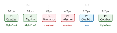
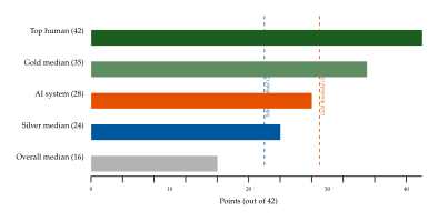
Technical Deep Dive: MCTS for Lean Proof Search
We now provide a more detailed treatment of how MCTS is adapted for proof search in the Lean environment, highlighting the key modifications relative to the game-playing setting.
The Proof Search Tree
In AlphaZero for Go, the search tree has a simple structure: each node is a board position, and each edge is a legal move. In AlphaProof, the structure is more complex:
Definition 24 (Proof Search Tree).
A proof search tree consists of:
A set of nodes , where each node corresponds to a proof state: a tuple where is the list of open goals (propositions to be proved) and is the local context (hypotheses, definitions, and intermediate results available for use).
A set of directed edges , where indicates that proof state can be reached from by applying a single Lean tactic.
A root node corresponding to the initial proof state (the original theorem statement as the single open goal, with the global Lean environment as the context).
Terminal nodes are proof states where (all goals closed; proof complete) or states from which no applicable tactic can make progress (dead ends).
The branching factor at each node depends on the number of applicable tactics. For a typical proof state, the “raw” branching factor (the total number of syntactically valid tactic applications) may be in the thousands. The policy network's role is to reduce this effective branching factor by assigning high probabilities to a small number of promising tactics and near-zero probabilities to the rest.
Handling Variable-Length Actions
In Go, each action is a simple board position (a single integer specifying the intersection to play). In Lean, a tactic can be an arbitrarily complex string, such as:
apply Nat.le_of_dvd (Nat.pos_of_ne_zero h1)
(Nat.dvd_trans h2 h3)
This means the “action space” is not a fixed finite set but the space of all valid tactic strings. AlphaProof addresses this by using the language model to generate tactic strings autoregressively, token by token, conditioned on the current proof state. The policy is thus implemented as: (Tactic GEN) where is the sequence of tokens comprising the tactic, and is the proof state. During MCTS, the language model generates a set of candidate tactics via beam search or sampling, and these candidates become the children of the current node.
Value Network Design
The value network estimates the probability that the proof can be completed from state . This is challenging because:
The distribution of proof lengths is highly skewed: some proofs require 3 tactics, while others require 300.
The value can change dramatically with a single tactic: a proof state that looks hopeless may become trivial after the right lemma is applied.
There is no natural “opponent” to calibrate the value against (unlike in two-player games where the value represents the probability of winning against a specific opponent).
In practice, the value network is trained on binary labels: for proof states that lie on a path to a completed proof, and for proof states from which no proof was found within the search budget. This introduces a subtle bias: states labelled may actually be provable with more search, and states labelled may only be provable via a specific, hard-to-find path.
The Modified PUCT Algorithm
AlphaProof uses a modified version of the PUCT (Polynomial Upper Confidence Trees) algorithm used in AlphaZero. The key modifications include:
Progressive widening. Rather than expanding all children of a node simultaneously (which would require generating all possible tactics), AlphaProof expands children incrementally: when a node is visited for the -th time, a new child may be added if exceeds a threshold that grows sublinearly with the number of existing children.
Proof-state deduplication. Different tactic sequences can lead to the same proof state. AlphaProof maintains a hash table of visited proof states and merges duplicate nodes in the search tree, converting it into a directed acyclic graph (DAG).
Tactic verification caching. Since each tactic application requires calling the Lean type checker (which can be computationally expensive), results are cached to avoid redundant verification.
Backpropagation with proof completion. When a proof is completed at a leaf node, the value is backpropagated to all ancestors, which updates their -values and biases future search towards the successful branch.
Exercises for Section 14
Exercise 72.
Consider the UCT formula from (UCT). Suppose a node has three children with the following statistics:
| Action | |||
| 0.7 | 10 | 0.5 | |
| 0.9 | 2 | 0.3 | |
| 0.0 | 0 | 0.2 |
Compute the UCT score for each action.
Which action would be selected?
How does the answer change if (low exploration) versus (high exploration)?
Explain intuitively why the UCT formula balances exploitation and exploration.
Exercise 73.
Definition 23 casts theorem proving as a single-player game. Extend this analogy by considering the following:
What is the “branching factor” of the proof game? How does it compare to Go (250) and chess (35)?
In two-player games, the value function estimates the probability of winning against the opponent. In the proof game, what does estimate, and what plays the role of the “opponent”?
AlphaZero uses self-play to generate training data. What is the analogue of “self-play” in the proof setting?
One advantage of theorem proving over board games is perfect verification. Explain why this is important for the training loop and how it affects the quality of the reward signal.
Exercise 74.
Consider the following competition problem: “Prove that for every positive integer , the number is divisible by 6.”
Write a formal statement of this theorem in Lean-like pseudocode (you do not need exact Lean syntax).
Identify at least two different proof strategies that could be represented as tactic sequences.
Estimate the depth of the proof search tree for each strategy (i.e., the number of tactic applications needed).
Which strategy do you think AlphaProof's MCTS would be more likely to discover, and why?
Exercise 75.
Curriculum design is critical for AlphaProof's training. Propose a curriculum strategy for training a theorem prover on number theory:
List ten theorems in rough order of increasing difficulty, from basic divisibility to Olympiad-level number theory.
Describe how you would measure the “difficulty” of a theorem for the purposes of curriculum scheduling.
What happens if the curriculum is too easy? Too hard?
Propose a method for automatically generating new theorems of intermediate difficulty (hint: consider perturbations of known theorems).
Exercise 76.
AlphaGeometry generates synthetic geometry training data by randomly sampling geometric configurations and deriving consequences.
Describe a simple version of this process for triangle geometry: what objects would you sample, what constraints would you impose, and what deduction rules would you apply?
Why is it important that the synthetic data includes auxiliary constructions as training targets?
What are the limitations of training on synthetic data? Can you think of geometry problems that might require reasoning patterns not captured by the synthetic generation process?
Propose an extension of the synthetic data generation process to handle problems involving three-dimensional geometry.
The Broader DeepMind AI for Math Ecosystem
AlphaProof and AlphaGeometry are the most visible components of DeepMind's AI for mathematics programme, but they are part of a much broader ecosystem of research projects that collectively represent the most ambitious effort to date to use artificial intelligence as a tool for mathematical discovery. In this section, we survey this ecosystem, examine the key projects, and compare DeepMind's approach with those of other major players in the field.
AlphaEvolve and Mathematical Discovery
In May 2025, DeepMind announced AlphaEvolve, an evolutionary coding agent powered by large language models [139]. While AlphaEvolve was not designed specifically for mathematics, several of its most striking results have direct mathematical significance.
AlphaEvolve uses an evolutionary framework in which a population of programs is maintained, with large language models (Gemini models of various sizes) serving as the mutation operators. Given a problem specification and an evaluation function, the system iteratively generates candidate programs, evaluates them, selects the best, and uses the LLM to produce variations. This process combines the open-ended creativity of LLMs with the rigorous evaluation of a fitness function, providing a form of “verified generation” that avoids the hallucination problems of pure LLM-based approaches.
Connection to Mathematics: Algorithm Discovery
AlphaEvolve's mathematical contributions have come primarily through the discovery of improved algorithms for well-studied computational problems. These algorithmic improvements often have deep connections to pure mathematics:
Matrix multiplication. The complexity of matrix multiplication is one of the central open problems in theoretical computer science. Strassen's 1969 algorithm showed that two matrices can be multiplied in operations, better than the naive . The current best exponent (due to Alman and Williams, 2024) is approximately . AlphaEvolve discovered new decompositions for small matrix multiplication problems (e.g., matrices) that improve upon previously known results, extending earlier work by AlphaTensor [48].
Sorting networks. AlphaEvolve found improved sorting networks for specific input sizes, in some cases matching or improving upon results that had stood for decades.
Kissing numbers and sphere packing. AlphaEvolve discovered improved constructions for kissing number problems in high dimensions, a classical topic in discrete geometry with connections to error-correcting codes and information theory.
Key Idea.
AlphaEvolve demonstrates a new paradigm for mathematical discovery: AI as a generator of candidate solutions that are rigorously evaluated by deterministic criteria. Unlike pure theorem proving (where the AI must produce a logically valid proof), AlphaEvolve's mathematical contributions come through constructive existence proofs: it finds examples (e.g., specific matrix multiplication algorithms) that establish the existence of solutions better than those previously known.
The AI for Math Initiative (October 2025)
In October 2025, Google DeepMind announced a major partnership with five of the world's leading mathematical research institutions to accelerate mathematical discovery using AI [140]. The participating institutions included research centres renowned for their contributions to pure mathematics, applied mathematics, and theoretical computer science.
The initiative has several stated goals:
Attacking open problems. Deploying DeepMind's AI systems (AlphaProof, AlphaGeometry, and related tools) to make progress on long-standing open problems in mathematics, including problems in number theory, combinatorics, algebraic geometry, and analysis.
Developing new AI tools for mathematicians. Creating interactive AI assistants that can help mathematicians explore conjectures, verify proofs, and discover new results. The goal is not to replace mathematicians but to augment their capabilities, acting as a “tireless collaborator” that can perform tedious calculations, check edge cases, and suggest proof strategies.
Formalising mathematics at scale. Accelerating the formalisation of existing mathematical knowledge in Lean, which would create both a verified record of mathematical results and a larger training corpus for AI proof systems.
Understanding the limits of AI-driven mathematics. Investigating which kinds of mathematical problems are amenable to AI approaches, which require fundamental advances in AI capabilities, and which (if any) are inherently beyond the reach of computational methods.
Remark 33.
The AI for Math Initiative represents a significant shift in the relationship between AI research and pure mathematics. For most of the history of AI, mathematics served as a tool for AI (providing the theoretical foundations for learning algorithms, optimisation methods, and statistical inference). The initiative inverts this relationship: AI becomes a tool for mathematics, a computational microscope through which mathematicians can examine structures too complex for human intuition alone.
The Aletheia Project
The Aletheia project represents perhaps the most philosophically significant of DeepMind's AI for mathematics efforts: the use of large language models, specifically Gemini, to attack genuine open research problems in mathematics, problems whose answers are unknown even to human experts.
Approach: Structured Exploration with Verification
The Aletheia methodology represents a carefully designed protocol for using LLMs as mathematical research tools [141]. The key insight is that LLMs, despite their tendency to hallucinate, can serve as powerful hypothesis generators when combined with rigorous verification:
Problem formulation. A human mathematician formulates an open problem and provides background context: relevant definitions, known results, failed attempts, and conjectured approaches.
Structured prompting. The LLM is prompted to explore the problem systematically, generating conjectures, proof sketches, and counterexample candidates. The prompting is structured to encourage step-by-step reasoning and to explicitly flag uncertain steps.
Verification loop. Each claim made by the LLM is verified by the human mathematician (and, where possible, by formal verification in Lean). Verified claims become new premises for further exploration; refuted claims become constraints that guide the search away from dead ends.
Iterative refinement. The process iterates, with the human mathematician steering the exploration based on mathematical judgement while the LLM provides computational breadth, exploring many more possibilities than a human could in the same time.
Case Study: The BKKKZ26 Result
One of the most striking results from the Aletheia project is a generalisation of irrationality results for rapidly converging series, referred to as the BKKKZ26 result (after the initials of the research team) [141].
The classical theory of irrationality, dating back to Euler and Liouville, provides criteria for determining when certain infinite series produce irrational numbers. A well-known example is the sum , which converges to and is irrational. More generally, series of the form , where and are integer sequences with specific growth properties, are known to be irrational under various conditions.
The BKKKZ26 result, discovered through the Aletheia methodology, established a new and more general criterion for the irrationality of such series. The key steps in the discovery were:
The human mathematician identified a class of series for which existing irrationality criteria were insufficient.
Gemini was prompted to explore generalisations of the known criteria, producing several candidate generalisations.
Most candidates were quickly refuted by counterexamples (some found by the LLM itself, others by the human mathematician).
One candidate survived all attempts at refutation and was eventually proved correct by the human mathematician, with the LLM assisting in the verification of several technical lemmas.
Remark 34.
The BKKKZ26 result illustrates a recurring pattern in LLM-assisted mathematical discovery: the AI does not produce the final proof, but it plays a crucial role in the exploration phase, generating the conjecture that the human mathematician then proves. This is analogous to how experimental physicists and theoretical physicists collaborate: one generates data and observations, the other provides explanations and proofs.
Solving Erdos Problems
Paul Erdos, one of the most prolific mathematicians of the 20th century, was famous for posing hundreds of open problems, often attaching cash prizes to them. Many of these problems remain open decades after his death in 1996. The Aletheia project has made progress on several Erdos problems, using the structured exploration methodology described above [141].
While the details of specific results are beyond the scope of this chapter, the significance is clear: AI systems are now capable of contributing to the resolution of problems posed by one of history's greatest mathematical minds. The problems solved are not trivial exercises but genuine research questions that resisted decades of effort by human mathematicians.
Google's Approach vs. OpenAI's Approach vs. DeepSeek's Approach
The three most significant players in AI for mathematics as of 2025 are Google DeepMind, OpenAI, and DeepSeek. Each has adopted a distinctive philosophy, and comparing them illuminates the key design choices facing the field.
Google DeepMind: RL-Heavy, Formal Verification, Massive Compute
Google DeepMind's approach, exemplified by AlphaProof, is built on three pillars:
Reinforcement learning. The AlphaZero paradigm of self-play RL is the core training methodology. The key bet is that RL can discover proof strategies that are not present in any existing training corpus.
Formal verification. All proofs are verified by the Lean type checker, providing a guarantee of correctness that is absent from natural-language proof systems. This allows the training loop to use a clean binary reward signal (proof correct or not), which is essential for RL.
Massive test-time compute. The system invests enormous computational resources at inference time (days of TPU time per problem). This reflects a belief that mathematical reasoning requires deep search, and that scaling compute at test time (not just training time) is the key to solving harder problems.
OpenAI: Reasoning Models and Chain-of-Thought
OpenAI's approach to mathematical AI is built around reasoning models: large language models (the o-series: o1, o3, o4-mini) that have been trained to produce extended chain-of-thought reasoning before arriving at an answer [112][113].
The key features of OpenAI's approach are:
Natural language reasoning. Rather than operating in a formal language like Lean, the o-series models reason in natural language (or a structured form of it), producing step-by-step arguments that are evaluated by human judges or automated checkers.
Reinforcement learning from human feedback (RLHF) and verification. The models are trained using RLHF, with the reward signal coming from the correctness of the final answer (for problems with known answers) or from human evaluation of the reasoning chain.
Scaling via chain length. The models can produce very long chains of thought (tens of thousands of tokens), and performance tends to improve with longer chains. This is a form of test-time compute scaling, but it operates within the autoregressive generation framework rather than the tree search framework of AlphaProof.
“First Proof?” claims. OpenAI has claimed that its o-series models have produced novel mathematical results, including what it describes as “first proofs” of previously unproven statements. These claims are controversial: without formal verification, it is difficult to distinguish genuine novel proofs from correct-sounding but flawed arguments.
The strengths and weaknesses of the OpenAI approach are complementary to those of AlphaProof. Chain-of-thought reasoning produces proofs in natural language that are (in principle) readable by human mathematicians, which is a significant advantage for communication and understanding. However, the lack of formal verification means that the correctness of the proofs cannot be guaranteed: subtle errors in reasoning, especially in long chains of inference, can escape detection by both the model and human reviewers. The OpenAI approach also scales differently: while AlphaProof can invest arbitrary compute in deepening the search tree, the o-series models are limited by the maximum context length and the diminishing returns of ever-longer chains of thought.
DeepSeek: GRPO, Open Models, and DeepSeek-Prover
DeepSeek, the Chinese AI company, has emerged as a significant player in AI for mathematics through its open-source models and novel training methodologies:
Group Relative Policy Optimization (GRPO). DeepSeek developed GRPO as an alternative to PPO and RLHF for training mathematical reasoning models. GRPO groups together multiple model outputs for the same problem, ranks them by correctness, and updates the model to increase the probability of correct outputs relative to incorrect ones [49]. This is conceptually related to rejection sampling fine-tuning but operates at the policy-gradient level.
Open models. Unlike Google and OpenAI, DeepSeek releases its models as open-source, including DeepSeek-Prover [4], a model specifically trained for formal theorem proving in Lean. DeepSeek-Prover has achieved strong results on the miniF2F benchmark and on Lean formalization tasks.
Lean integration. DeepSeek-Prover, like AlphaProof, operates within the Lean formal verification framework, but uses a different search strategy: rather than MCTS, it generates complete proof attempts autoregressively and verifies them, using a generate-and-verify loop with multiple sampling.
| Aspect | Google DeepMind | OpenAI | DeepSeek |
| Core method | RL + MCTS | Chain-of-thought | GRPO |
| Verification | Lean (formal) | Natural language | Lean (formal) |
| Search strategy | Tree search | Sequential gen. | Generate-verify |
| Compute scaling | Test-time MCTS | Chain length | Sample count |
| Key system | AlphaProof | o3/o4-mini | DeepSeek-Prover |
| Open source | No | No | Yes |
| IMO results | 28/42 (2024) | N/A | N/A |
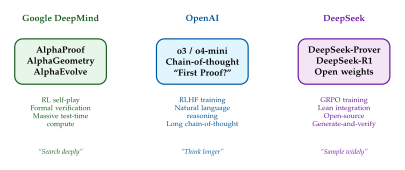
Connection to AlphaFold: Structure Prediction as a Unifying Theme
At first glance, AlphaFold (DeepMind's protein structure prediction system) and AlphaProof (its theorem proving system) seem to belong to entirely different domains. One deals with biology, the other with mathematics. One predicts three-dimensional molecular structures, the other constructs logical arguments. Yet the two systems share deep structural similarities that illuminate a general principle of DeepMind's research programme.
The Shared Architecture: Search + Learning
Both AlphaFold and AlphaProof can be understood as instances of a common pattern: structure prediction as search + learning.
Definition 25 (Structure Prediction Problem).
A structure prediction problem consists of:
An input specification (a protein amino acid sequence for AlphaFold; a theorem statement for AlphaProof).
A structured output (a 3D atomic coordinate set for AlphaFold; a tactic-level proof for AlphaProof).
A verification criterion (comparison with experimentally determined structures for AlphaFold; type checking in Lean for AlphaProof).
A search space that is combinatorially vast (the space of possible 3D conformations; the space of possible tactic sequences).
Both systems address the combinatorial explosion of the search space through the same strategy: train a neural network to provide approximate but fast evaluations, then use these evaluations to guide a structured search process.
Key Differences
Despite the structural similarities, there are important differences:
Nature of verification. AlphaFold's predictions are verified against experimental data (X-ray crystallography, cryo-EM), which is noisy, incomplete, and expensive to obtain. AlphaProof's proofs are verified by the Lean type checker, which is deterministic, complete, and computationally cheap. This difference profoundly affects the training dynamics: AlphaProof can generate its own training labels through RL (every proof attempt is either verified or not), while AlphaFold depends on a fixed corpus of experimentally determined structures.
Nature of the output. AlphaFold's output (a set of 3D coordinates) is continuous and can be refined by gradient descent. AlphaProof's output (a sequence of tactics) is discrete and must be constructed combinatorially.
Training paradigm. AlphaFold is trained primarily by supervised learning on known protein structures (with some self-distillation). AlphaProof is trained by a combination of supervised pre-training and reinforcement learning.
Failure mode. AlphaFold can produce a “wrong” structure that is still physically plausible (a low-energy conformation that happens not to be the native state). AlphaProof either finds a correct proof (verified by Lean) or fails entirely; there is no “approximately correct proof.”
Key Idea.
The connection between AlphaFold and AlphaProof suggests a general research programme: identify domains where the output has rich combinatorial structure, where fast approximate evaluation can be learned, and where verification is possible (either experimentally or formally). Such domains are natural targets for the “search + learning” paradigm. Potential future applications include drug design, materials science, program synthesis, and circuit design.
The DeepMind AI for Math Ecosystem: A Unified View
We can now step back and view DeepMind's AI for mathematics projects as components of a coherent ecosystem, each addressing a different aspect of mathematical practice.
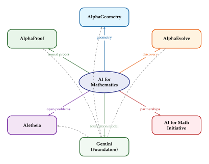
AlphaProof: formal theorem proving via RL and MCTS in Lean. Addresses the verification aspect of mathematics: given a statement, produce a certified proof.
AlphaGeometry: neuro-symbolic geometry reasoning. Addresses the domain-specific aspect: exploiting the structure of Euclidean geometry for efficient reasoning.
AlphaEvolve: evolutionary algorithm discovery. Addresses the constructive aspect: finding specific objects (algorithms, configurations) that establish existence results.
Aletheia: LLM-assisted exploration of open problems. Addresses the creative aspect: generating conjectures and proof strategies for problems whose solutions are unknown.
AI for Math Initiative: institutional partnerships. Addresses the social aspect: connecting AI capabilities with mathematical expertise and embedding AI tools in the mathematical research community.
Gemini: the foundation model that underpins multiple components (autoformalization in AlphaProof, the neural model in AlphaGeometry 2, the mutation operator in AlphaEvolve, the exploration engine in Aletheia).
Together, these components span the full range of mathematical practice: from routine verification to creative discovery, from domain-specific reasoning to general-purpose proof search, from individual problem-solving to community-scale collaboration.
Remark 35.
The ecosystem view also reveals a dependency structure. Gemini is the foundation on which everything else is built. Improvements to Gemini's mathematical reasoning capabilities propagate upward to all systems that use it. Conversely, the specialised systems (AlphaProof, AlphaGeometry) generate training data and insights that can improve Gemini's general mathematical capabilities. This creates a flywheel effect: better foundation models enable better specialised systems, which generate better data for training foundation models.
Open Challenges and Future Directions
Despite the remarkable progress described in this section, several fundamental challenges remain:
The Formalization Bottleneck
AlphaProof's reliance on the Lean formal language means that problems must be formalised before the system can attack them. Autoformalization is improving rapidly, but it remains error-prone for complex statements involving advanced mathematical concepts. The gap between the mathematics that can be stated informally and the mathematics that can be formalised automatically is still significant.
Moreover, the Mathlib library, while large, covers only a fraction of modern mathematics. Many active research areas (e.g., algebraic geometry beyond the basics, advanced homotopy theory, analytic number theory) have little or no Lean formalisation, making them largely inaccessible to AlphaProof.
Compute Requirements
AlphaProof's three-day compute budget for a single IMO problem is enormous. Scaling to harder problems (e.g., research-level theorems in algebraic geometry or analytic number theory) may require even more compute. If the scaling law in (Testtime Scaling) holds, the compute requirements for problems of increasing difficulty will grow exponentially.
Mathematical Creativity
The most profound open question is whether AI systems can exhibit genuine mathematical creativity: the ability to introduce entirely new concepts, definitions, and proof techniques that are not present in the training data. AlphaProof's RL training can discover new proof strategies by combining known tactics in novel ways, but this is combinatorial creativity (recombination of existing elements), not conceptual creativity (invention of new elements).
The greatest mathematical breakthroughs, from Cantor's transfinite numbers to Grothendieck's schemes to Thurston's geometrisation programme, involved the creation of entirely new mathematical frameworks. Whether AI can achieve this kind of creativity remains one of the deepest open questions in the field.
Interpretability and Understanding
When AlphaProof produces a proof, the proof is verifiably correct (Lean guarantees this), but it may not be understandable by human mathematicians. Long, computer-generated proofs can be correct but opaque, providing no insight into why the theorem is true. For mathematics as a human endeavour, understanding is at least as important as verification.
Developing AI systems that produce not just correct proofs but illuminating proofs, proofs that reveal the underlying structure and suggest generalisations, is a major open challenge.
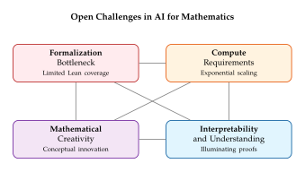
Exercises for Section 15
Exercise 77.
AlphaEvolve uses LLMs as mutation operators in an evolutionary framework.
Compare this approach with traditional evolutionary programming (where mutations are random perturbations). What advantages does LLM-guided mutation provide?
Why is a fitness function essential for AlphaEvolve's mathematical contributions? What would happen if the fitness function were replaced by a neural network reward model?
Propose an AlphaEvolve-style approach for discovering improved algorithms for fast Fourier transforms (FFTs). What would the program representation, fitness function, and mutation strategy look like?
Discuss the relationship between AlphaEvolve's “constructive existence proofs” and the traditional mathematical notion of proof. Is finding a better algorithm a form of theorem proving?
Exercise 78.
The Aletheia project uses a “structured exploration with verification” methodology.
Design a simplified version of this methodology for exploring conjectures in graph theory. Describe the roles of the human mathematician and the AI system at each stage.
What are the risks of using LLMs as hypothesis generators? How does the verification step mitigate these risks?
The BKKKZ26 result involved generalising known irrationality criteria. Propose a general framework for using LLMs to generate mathematical generalisations: given a theorem with conditions , how would you prompt an LLM to explore weaker conditions under which still holds?
Compare the Aletheia methodology with the traditional mathematical research process. What aspects of mathematical research are well-suited to AI assistance, and what aspects are not?
Exercise 79.
Table 7 compares three approaches to AI for mathematics.
For each of the following mathematical tasks, argue which approach (Google, OpenAI, or DeepSeek) is best suited and why: itemize
Proving a theorem in commutative algebra.
Discovering a counterexample to a graph theory conjecture.
Generating a clear, human-readable proof of an elementary number theory result.
Solving a high-school mathematics competition problem. itemize
The three approaches emphasise different forms of test-time compute scaling: tree search depth (Google), chain length (OpenAI), and sample count (DeepSeek). Derive informal scaling laws for each: how does the probability of finding a correct proof scale with the compute budget under each strategy?
Propose a hybrid system that combines the strengths of all three approaches. How would it handle each of the tasks in part (a)?
Exercise 80.
The connection between AlphaFold and AlphaProof (Connection to AlphaFold: Structure Prediction as a Unifying Theme) suggests a general “search + learning” paradigm for structure prediction.
Identify three domains outside of biology and mathematics where the “search + learning” paradigm could be applied. For each, describe the input specification, structured output, verification criterion, and search space.
For one of your proposed domains, design (at a high level) a system analogous to AlphaProof. What would the “tactics” be? What would the “value network” estimate?
What properties of a domain make it particularly well-suited to the “search + learning” approach? What properties make it poorly suited?
The key difference between AlphaFold and AlphaProof is the nature of verification (experimental vs. formal). How does this difference affect the training paradigm, the scaling behaviour, and the trustworthiness of the outputs?
Exercise 81.
The formalization bottleneck (The Formalization Bottleneck) is one of the key limitations of formal AI-driven mathematics.
Estimate the fraction of modern mathematical research that could currently be formalised in Lean (based on Mathlib's coverage). Which areas are well-covered? Which are essentially absent?
Propose a strategy for accelerating the formalisation of mathematics. Consider both human-driven approaches (better tools, incentive structures) and AI-driven approaches (autoformalization, synthetic data generation).
What would it take to formalise a typical research paper in algebraic geometry? Estimate the effort in person-months.
Discuss the social and institutional barriers to mathematical formalisation. Why have most mathematicians not adopted formal proof assistants, despite their advantages?
Exercise 82.
Mathematical creativity (Mathematical Creativity) is arguably the hardest challenge for AI.
Define “mathematical creativity” as precisely as you can. Is it the same as “producing outputs not in the training data,” or is something more required?
Give three examples of mathematical breakthroughs that involved genuine conceptual innovation (the creation of new mathematical objects or frameworks). For each, argue whether the innovation could, in principle, have been produced by an RL-trained system.
Propose a test for mathematical creativity analogous to the Turing test. What would the AI need to do to pass?
Some philosophers argue that mathematical creativity requires “understanding” in a sense that AI systems lack. Evaluate this argument in light of AlphaProof's IMO 2024 performance: does solving Problem 6 (which only five humans solved) constitute evidence of understanding?
Exercise 83.
AlphaProof produces correct but potentially opaque proofs.
Define what makes a proof “illuminating” versus merely “correct.” Give an example of a theorem with both an illuminating proof and a correct but opaque proof.
Propose a method for post-processing a computer-generated proof to make it more human-readable. What information would you need, and what transformations would you apply?
Design a metric for “proof quality” that captures readability, elegance, and explanatory power, in addition to correctness. How could this metric be used as a training signal for an AI proof system?
The four-colour theorem (1976) and the Kepler conjecture (2014) were proved with substantial computer assistance, and both proofs were controversial in the mathematical community. Research these cases and discuss how the interpretability challenge will intensify as AI-generated proofs become more common.
Exercise 84.
Design (at a high level) an AI system for solving mathematical competition problems that combines ideas from all three approaches discussed in Google's Approach vs. OpenAI's Approach vs. DeepSeek's Approach.
Describe the architecture: what components would you include, and how would they interact?
What training data and training procedure would you use?
How would the system handle different mathematical domains (algebra, combinatorics, geometry, number theory)?
What would the inference procedure look like? How would you allocate compute across the components?
Estimate the computational resources needed to match human gold medal performance at the IMO.
OpenAI's Path to Mathematical Reasoning
While DeepMind pursued formal methods through AlphaProof, OpenAI charted a different course: scaling natural-language reasoning to the point where models could tackle research-level mathematics without formal verification as a crutch. The results, culminating in GPT-5.4 Pro's performance on FrontierMath, have been nothing short of transformative.
GPT-4 and Early Mathematical Capabilities
When GPT-4 was released in March 2023, its mathematical abilities were already striking: it scored in the 90th percentile on the AP Calculus exam and solved roughly 42% of problems on the MATH benchmark [118]. Yet careful analysis revealed systematic weaknesses.
Example 46 (GPT-4's Strengths and Weaknesses).
Strength. GPT-4 excels at pattern-matching familiar problem types:
Problem: Find . GPT-4: Using the formula , we get . ✓
Weakness. GPT-4 struggles with novel constructions:
Problem: Prove that the group of units of is cyclic if and only if or for odd prime . GPT-4: [Produces a plausible but subtly flawed argument, missing the case analysis for .]
Key Idea.
GPT-4's mathematical reasoning operates through pattern completion: it recognises problem templates from training data and fills in the details. This works well for standard exercises but fails when genuine creativity or novel construction is required.
Chain-of-thought (CoT) prompting [11] significantly improved GPT-4's mathematical performance by encouraging the model to decompose problems into explicit steps, mimicking the scratchpad work of human problem solvers.
The Reasoning Revolution: o-Series Models
In September 2024, OpenAI released o1, inaugurating a new paradigm: reasoning models that spend additional compute at inference time to think through problems step by step.
Definition 26 (Test-Time Compute Scaling).
A reasoning model allocates variable compute at inference time by generating an internal chain of thought before producing its final answer. The key insight is that mathematical performance scales with the amount of compute spent “thinking”: where is the number of reasoning tokens and are task-dependent constants.
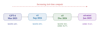
The o-series models introduced several key innovations:
Internal chain of thought: The model generates a hidden reasoning trace before producing its answer. This trace can be thousands of tokens long for hard problems.
Self-verification: The model checks its own work, backtracking when it detects errors in its reasoning.
Exploration: For difficult problems, the model explores multiple solution strategies in parallel, selecting the most promising.
Remark 36.
The o3 model achieved a score of 96.7% on the 2024 AIME (American Invitational Mathematics Examination), surpassing all but the very best human competitors. On the MATH benchmark, o3 scored 96.1%, approaching saturation.
GPT-5.4 Pro: The State of the Art
GPT-5.4 Pro, released in early 2026, represents the current frontier of natural-language mathematical reasoning.
Historical Note.
When the FrontierMath benchmark was released in November 2024, no AI system scored above 2% on research-level problems. The benchmark's creators (including Terence Tao) expected it to remain unsolved for years. Within sixteen months, GPT-5.4 Pro achieved approximately 47.6% on Tiers 1 through 3, a rate of progress that stunned the mathematical community [50].
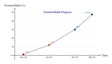
The Graviton Amplitude Discovery
Perhaps the most remarkable mathematical contribution from OpenAI's models was not a proof but a discovery. In February 2026, physicists Alfredo Guevara, Alexandru Lupsasca, David Skinner, and Andrew Strominger, working with GPT-5.2 Pro, overturned a decades-old assumption in theoretical physics [142].
The story begins with a standard question: are single-minus tree-level scattering amplitudes zero? For decades, the answer was believed to be “yes” for any number of external particles.
Insight.
GPT-5.2 Pro produced a formula using the directed matrix-tree theorem that the researchers initially dismissed as a hallucination. When they ran symbolic verification against known lower-order results and numerical simulations, every check confirmed the formula. The AI had found a genuine, previously unknown result that contradicted decades of assumed physics.
We defer the full technical treatment to The Graviton Amplitude Discovery, where we present the mathematical details and discuss the profound implications for the relationship between hallucination and creativity.
Contrast with DeepSeek
OpenAI and DeepSeek represent two fundamentally different philosophies for mathematical AI:
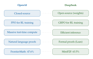
Definition 27 (Group Relative Policy Optimisation (GRPO)).
DeepSeek's GRPO [51] eliminates the value function from PPO. Given a prompt and a group of sampled responses with rewards , the advantage is estimated as: The policy gradient update is:
Proposition 4 (GRPO Advantage Estimator is Unbiased).
The group-relative advantage estimator is an unbiased estimator of the centred reward: .
Proof.
By linearity of expectation, as . The normalisation by preserves the sign and relative ordering. The centring ensures that , which stabilises the policy gradient.
The Competition Landscape
The period from 2024 to 2026 witnessed an extraordinary proliferation of companies and systems competing to solve mathematics with AI. We survey the major players, their architectures, and their results.
Axiom Math
Axiom Math, founded in San Francisco in July 2025, has emerged as perhaps the most impressive player in AI for formal mathematics. Their results on the Putnam competition shook the mathematical world.
Historical Note.
The William Lowell Putnam Mathematical Competition, held annually since 1938, is widely regarded as the most prestigious undergraduate mathematics competition in North America. In its 98-year history, only five humans had ever achieved a perfect score of 120 points (12 problems, 10 points each). In December 2025, Axiom's system scored 120/120, becoming the first AI to achieve a perfect Putnam score [52].
The Axiom pipeline consists of four components:
Definition 28 (AXLE Pipeline).
The Axiom Lean Engine (AXLE) pipeline:
Auto-formaliser: Translates natural-language problems into Lean 4 statements.
Conjecturer: Proposes intermediate lemmas that may assist the proof.
Prover: Assembles the complete proof, with every step checked by Lean's compiler-grade verifier.
Auto-informaliser: Translates the verified Lean proof back to human-readable LaTeX/English.
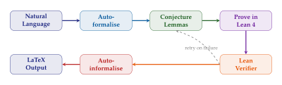
In February 2026, Axiom announced solutions to two open problems in number theory and algebraic geometry:
Removing a missing number-theoretic hypothesis that kept a parity result conditional, enabling its unconditional use in moduli space geometry.
Proving a theorem connecting to the partial Vandiver theorem, with consequences for -adic -functions, congruences between cusp forms and Eisenstein series, and -torsion in algebraic -groups.
Remark 37.
Axiom raised $200 million in a Series A round led by Menlo Ventures in March 2026, at a $1.6 billion post-money valuation. Their thesis: “AI will write all code; mathematics will prove it works.” This positions formal verification not just as a tool for pure mathematics but as critical infrastructure for verifying AI-generated software [52].
Harmonic's Aristotle
Harmonic AI's Aristotle system combines three components into a unified theorem-proving agent [143]:
Lean proof search: A transformer-based policy and value network, trained via RL expert iteration.
Informal reasoning: Natural-language decomposition of problems into subproblems.
Geometry solver: A dedicated module for geometric reasoning (following the AlphaGeometry paradigm).
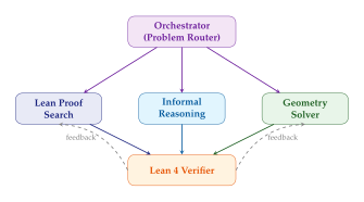
Key results:
90% on the MiniF2F benchmark (the first system to cross 90%).
IMO gold-level performance in 2025 (solving 5 of 6 problems).
Co-solved Erdos Problem #728 with Kevin Barreto and GPT-5.2 Pro.
Mistral's Leanstral
On March 16, 2026, Mistral AI released Leanstral, the first open-source Lean 4 theorem-proving agent.
Key Idea.
Leanstral demonstrates that competitive formal theorem proving does not require closed, proprietary systems. At 120 billion parameters with only 6 billion active (sparse mixture of experts), it achieves a Pass@2 score of 26.3 on MiniF2F, beating Claude Sonnet while costing $36 compared to Sonnet's $549 per run.
The release under the Apache 2.0 licence means researchers can:
Fine-tune Leanstral on domain-specific mathematics.
Integrate it into custom proof-search pipelines.
Study its internals to understand what the model has learned about mathematical reasoning.
Other Notable Systems
Math Inc.
Demonstrated the power of AI-assisted formalisation by completing the formalisation of the strong Prime Number Theorem in Lean 4 in just three weeks. This result had stalled for over 18 months of human effort, illustrating how AI can break through formalisation bottlenecks.
Apple's Hilbert.
Uses an innovative recursive architecture: informal reasoning produces a high-level proof sketch, which is recursively refined into formal Lean 4 steps. Each level of refinement is verified before proceeding to the next, ensuring that errors do not propagate.
Kimina-Prover (Mao et al., 2025).
An open-source system that combines a 72B language model with whole-proof generation (rather than individual tactic generation). Achieved state-of-the-art results on MiniF2F and ProofNet.
Comprehensive Comparison
| System | MiniF2F | MATH | AIME | Putnam |
| AlphaProof | 71.4% | - | 5/6 (IMO) | - |
| Aristotle | 90.0% | - | 5/6 (IMO) | - |
| Axiom/AXLE | - | - | - | 12/12 |
| GPT-5.4 Pro | - | 97.2% | 15/15 | - |
| DeepSeek-R1 | - | 97.3% | 79.2% | - |
| Leanstral | 26.3 (P@2) | - | - | - |
| Kimina-72B | 80.7% | - | - | - |
Remark 38.
Direct comparison across systems is difficult because they target different benchmarks and use different evaluation protocols. Some systems (AlphaProof, Axiom) produce formal proofs verified by Lean; others (GPT-5.4 Pro, DeepSeek) produce natural-language solutions checked by humans or grading scripts.
The MRAL Framework
DeepMind's “Towards Autonomous Mathematics Research” paper [144] proposed the Mathematical Research Autonomy Levels (MRAL) framework, modelled on self-driving car autonomy levels.
Definition 29 (MRAL Framework).
The MRAL framework classifies AI mathematical contributions along two axes:
Autonomy axis:
Level H: Human-led with secondary AI input.
Level C: Genuine human-AI collaboration.
Level A: Essentially autonomous AI research.
Significance axis:
Level 0: Trivial or already-known result.
Level 1: Publishable but incremental.
Level 2: Significant contribution to a field.
Level 3: Major result (e.g., resolving a well-known conjecture).
Level 4: Transformative (e.g., new theory, Fields Medal-level).
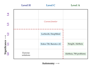
Remark 39.
The MRAL framework is important for calibrating expectations. As of March 2026, the highest-significance autonomous result is approximately Level A/L1 (Aletheia's Feng26 paper on eigenweights). Achieving Level A/L3 or above remains an open challenge.
Benchmark Landscape
| Benchmark | Level | Problems | Format |
| GSM8K | Grade school | 8.5K | Natural language |
| MATH | Competition | 12.5K | Natural language |
| MiniF2F | Competition | 488 | Lean/Isabelle |
| ProofNet | Undergraduate | 371 | Lean 4 |
| AIME | Competition | 15/year | Natural language |
| Putnam | Competition | 12/year | Natural language |
| PutnamBench | Competition | 644 | Lean 4 |
| FrontierMath | Research | 300+ | Natural language |
| First Proof | Research | 10 | Natural language |
Insight.
The field has rapidly saturated lower-level benchmarks: GSM8K is at near-100%, MATH is above 97%. The frontier has shifted to research-level benchmarks like FrontierMath and First Proof, where even the best systems solve less than half the problems. This “moving target” phenomenon ensures that benchmarks continue to drive progress.
Exercises
Exercise 85.
Compare the AXLE pipeline (Definition 28) with the standard compile-test loop in software engineering. What are the analogues of unit tests, integration tests, and code review?
Exercise 86.
The GRPO advantage estimator (Definition 27) normalises by . Explain what happens when and why the term is necessary.
Exercise 87.
Using the MRAL framework (Definition 29), classify the following AI mathematical achievements:
GPT-4 solving an AIME problem.
AlphaProof's IMO silver medal.
Axiom's Putnam perfect score.
Aletheia's Feng26 paper.
The graviton amplitude discovery.
Exercise 88.
(Challenge.) Design a benchmark for AI mathematical reasoning at the graduate level (between MATH and FrontierMath in difficulty). Specify: (a) the mathematical domains, (b) the difficulty criteria, (c) the evaluation protocol, and (d) measures to prevent data contamination.
Exercise 89.
Explain why Leanstral's sparse MoE architecture (120B total, 6B active parameters) is well-suited for theorem proving. What aspects of proof search benefit from expert specialisation?
Exercise 90.
(Research.) The MRAL framework has only three autonomy levels. Propose a finer-grained scale with at least five levels, giving a concrete example for each. How would you measure the autonomy level of a given system?
Exercise 91.
Compare the test-time compute scaling of reasoning models (Definition 26) with AlphaProof's test-time RL (which generates millions of problem variants during inference). Which approach is more sample-efficient? Which is more general?
Exercise 92.
(Essay.) Axiom's thesis is “AI will write all code; mathematics will prove it works.” Critically evaluate this claim. What are the main obstacles? Is formal verification of AI-generated code practical today?
The First Proof Benchmark
On February 5, 2026, eleven leading mathematicians released the most ambitious test of AI mathematical reasoning ever conceived: First Proof, a collection of ten research-level problems drawn from their own unpublished work [145]. Unlike competition benchmarks, where solutions exist in textbooks and training corpora, not a single solution to these problems had ever appeared in print, on the internet, or in any known dataset.
Key Idea.
First Proof was designed to answer a single question: can AI produce genuine mathematical research, or is it merely retrieving and recombining known solutions? By using problems from unpublished work by Fields medalists, the benchmark closes the data contamination loophole entirely.
The Problems and Their Creators
The problems were contributed by:
Martin Hairer (Fields Medal 2014): stochastic analysis.
Mohammed Abouzaid (Stanford): symplectic geometry.
Rachel Ward (UT Austin): numerical linear algebra.
Nikhil Srivastava (UC Berkeley): spectral graph theory.
Lauren Williams (Harvard): algebraic combinatorics.
The ten problems span:
Algebraic combinatorics (cluster algebras, positroid varieties).
Spectral graph theory (Ramanujan graphs, spectral gaps).
Algebraic topology (persistent homology, spectral sequences).
Stochastic analysis (regularity structures, rough paths).
Symplectic geometry (Fukaya categories, Lagrangian intersections).
Representation theory (quantum groups, crystal bases).
Lattices in Lie groups (arithmetic quotients).
Tensor analysis (low-rank approximation).
Numerical linear algebra (randomised algorithms).
A combinatorial problem bridging several areas.
Remark 40.
Each problem took its contributing mathematician weeks to months to solve. The proofs are at most five pages, but they require deep insight into the relevant mathematical structures. This is precisely the regime where pattern-matching fails and genuine understanding is needed.
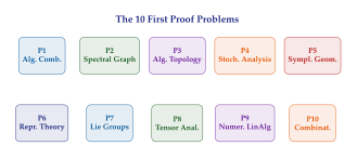
Results
On February 13, 2026, results were released:
OpenAI (GPT-5.2 Pro): solved 5 of 10 (Problems 4, 5, 6, 9, 10). Their attempt at Problem 2 was initially thought correct but was later found to contain a subtle flaw.
DeepMind (Aletheia): solved 6 of 10 by majority expert assessment.
Publicly available models (ChatGPT, Gemini): solved approximately 2 of 10.
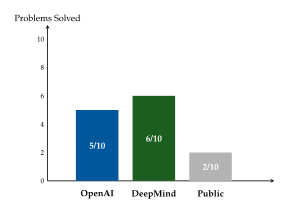
Analysis of Selected Solutions
Example 47 (Problem 4: A Stochastic Analysis Result).
Problem 4, contributed by Martin Hairer, asked for a regularity estimate in the theory of rough paths. The AI's approach was notable:
Problem recognition: The model correctly identified the problem as belonging to the theory of regularity structures, a framework developed by Hairer himself.
Key lemma: The model identified a crucial interpolation inequality that bridges the rough path regularity with classical Sobolev estimates.
Proof construction: Using this lemma, the model constructed a proof by induction on the regularity index, applying the reconstruction theorem at each step.
Insight.
The AI's solution to Problem 4 demonstrated genuine mathematical understanding: it did not merely apply a known template but identified the correct abstract framework and adapted it to a novel setting. Hairer himself described the proof as “clean and insightful.”
Example 48 (Problem 9: Numerical Linear Algebra).
Problem 9, contributed by Rachel Ward, concerned the convergence rate of a randomised sketching algorithm for least-squares problems.
The AI's solution introduced a novel decomposition of the error into “bias” and “variance” components: where is the projection onto the sketch subspace, is the problem dimension, is the sketch size, and bounds the noise.
The key insight was recognising that the Johnson–Lindenstrauss lemma could be applied not to the data points themselves but to the residual subspace, yielding a tighter bound than previous approaches.
What the Results Reveal
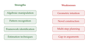
Key Idea.
The First Proof results suggest that current AI systems are at approximately the level of a talented postdoc: capable of solving problems within known frameworks but not yet able to create genuinely new mathematical structures or theories.
Exercises
Exercise 93.
Why is the First Proof benchmark fundamentally different from the MATH benchmark? Discuss at least three dimensions of difference.
Exercise 94.
OpenAI's solution to Problem 2 was initially thought correct but later found flawed. Discuss the challenges of evaluating research-level mathematical proofs. How might formal verification help?
Exercise 95.
(Challenge.) Read the First Proof paper (arXiv:2602.05192) and select one unsolved problem. Describe, at a high level, what mathematical tools might be relevant and why the problem is difficult.
Exercise 96.
The “bias-variance decomposition” in Problem 9's solution (Example 48) mirrors a classical concept in statistics. Explain the connection and why this decomposition is natural for randomised algorithms.
Case Study: Erdos Problems and AI
Paul Erdos (1913–1996) was the most prolific mathematician of the twentieth century, publishing over 1,500 papers and posing hundreds of open problems, many accompanied by cash bounties. His problems have driven decades of research in combinatorics, number theory, and graph theory.
Historical Note.
Erdos was famous for offering cash prizes for solutions to his
problems, ranging from $25 for easy problems to $10,000 for the
hardest. The Erdos Problems database
(erdosproblems.com) maintains a living catalogue of these
problems and their status. As of January 2026, hundreds remained open.
The Christmas 2025 Breakthrough
Beginning in late December 2025, a remarkable series of events unfolded: fifteen Erdos problems moved from “open” to “solved” in rapid succession, with eleven crediting AI involvement in some form [146].
Remark 41.
A careful analysis reveals that the AI contributions fell into three categories:
Literature search: The AI located existing published solutions that the database maintainer had not been aware of. (Approximately 4 of the 11.)
Standard technique application: The AI applied known techniques to specific problem formulations, producing correct but not deeply novel proofs. (Approximately 5 of the 11.)
Genuine insight: The AI contributed a key idea that was not a straightforward application of existing methods. (Approximately 2 of the 11.)
Case Study: Erdos Problem #728
The flagship case was Erdos Problem #728, solved on January 4, 2026, by Kevin Barreto using GPT-5.2 Pro and Harmonic's Aristotle system.
Definition 30 (Erdos Problem #728).
Show that for constants and , there exist infinitely many triples with such that
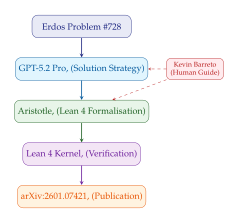
The solution approach.
The proof proceeds by:
Using properties of the -adic valuation (via Legendre's formula: ).
Showing that the divisibility condition is equivalent to a condition on binomial coefficients.
Constructing explicit triples using the theory of smooth numbers and the distribution of primes in arithmetic progressions.
Theorem 12 (Solution to Erdos Problem #728, Simplified).
For any and any positive constants , there exist infinitely many and pairs with and such that is an integer dividing .
Proof Sketch.
The key observation is that . For this to be an integer, we need . Setting in the range and choosing so that is a product of primes less than (a “smooth” number), the divisibility condition can be verified prime-by-prime using Kummer's theorem. The existence of infinitely many such smooth in the specified range follows from known results on smooth numbers.
Remark 42 (Tao's Assessment).
Terence Tao described this as “a near-autonomous solution that has not been reproduced in existing literature and represents a real improvement in AI capabilities.” However, he also noted that similar results using similar methods existed in a 2015 paper by Pomerance, and that these represent “lowest hanging fruit” among Erdos problems, solvable with standard techniques from analytic number theory.
Aletheia's Large-Scale Assessment
DeepMind's Aletheia system took a different approach: rather than targeting individual problems, it systematically evaluated 700 open problems from the Erdos database.
63 technically correct solutions were produced.
4 open questions were autonomously resolved (confirmed by expert review).
Many “solutions” were re-derivations of known results, demonstrating that the AI could independently reconstruct arguments from the literature.
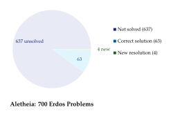
Lessons Learned
Key Idea.
The Erdos problem-solving episode reveals a crucial distinction: solving a problem (applying known techniques to a known formulation) is fundamentally different from discovering new mathematics (creating novel structures, definitions, or proof strategies). Current AI systems are approaching human-level at the former but remain far from the latter.
Insight.
The gap between “solving” and “discovering” mirrors a well-known phenomenon in human mathematics: many graduate students can solve problems using known techniques, but only a few develop the taste and creativity to identify and solve truly important problems. AI may need a similar leap.
Exercises
Exercise 97.
Explain Kummer's theorem and its relevance to the divisibility condition in Erdos Problem #728.
Exercise 98.
Why does Tao describe the solved Erdos problems as “lowest hanging fruit”? What would a “high-hanging” Erdos problem look like?
Exercise 99.
(Challenge.) Aletheia's assessment found 63 correct solutions out of 700 problems. If we model each problem as an independent Bernoulli trial with success probability , estimate and construct a 95% confidence interval. What does this tell us about the system's capability?
Exercise 100.
Discuss the ethical implications of AI solving problems with cash bounties. Who should receive the prize: the AI developer, the human guide, or the problem poser?
Exercise 101.
(Research.) Visit erdosproblems.com and select an
open problem. Can you identify the relevant mathematical techniques?
Formulate a strategy an AI might use and discuss what would make the
problem easy or hard for current systems.
Claude's Cycles: Solving Knuth's Graph Problem
In March 2026, Donald Knuth published a remarkable paper with a title that startled the computer science community: “Claude's Cycles.” The paper opened with “Shock! Shock!” and closed with a confession that would have been unthinkable from the father of algorithm analysis just a year earlier: “It seems I'll have to revise my opinions about generative AI one of these days” [147].
Historical Note.
Donald Knuth, author of The Art of Computer Programming and creator of , had been among the most prominent sceptics of AI's ability to do genuine mathematics. In a 2024 interview, he expressed doubt that language models could contribute anything beyond “plausible nonsense” to combinatorics. Claude's solution to a problem he had earmarked for a future volume of TAOCP forced him to reconsider.
The Problem
Definition 31 (Knuth's Hamiltonian Decomposition Problem).
Consider the directed graph on vertices, where vertices are elements of and directed edges connect each vertex to its neighbours under two generators. The problem: for all odd , find a decomposition of the vertex set into exactly three Hamiltonian cycles of length .
Knuth had solved the case by hand and verified solutions computationally up to , but no general construction existed for arbitrary odd dimensions.
The Solution Process
Filip Stappers, a colleague of Knuth, fed the problem statement to Claude Opus 4.6 and ran 31 guided explorations over approximately one hour. The transcript reveals a fascinating iterative process:
Linear formulas (Attempts 1–5): Claude first tried explicit coordinate formulas. These worked for but failed for .
Brute-force search (Attempts 6–10): Claude implemented backtracking search algorithms. These found solutions for small but did not generalise.
Geometric frameworks (Attempts 11–18): Claude explored lattice-based constructions, Gray codes, and space-filling curves. Several promising ideas hit dead ends.
Simulated annealing (Attempts 19–22): Claude switched to optimisation, using random perturbations to search for decompositions. This found solutions but provided no proof of generality.
The breakthrough (Attempts 23–31): Claude independently recognised the problem's underlying structure as a Cayley digraph with two generators and .
The Cayley Digraph Insight
The key breakthrough was recognising that the directed graph on is a Cayley digraph of the group with generators and .
Definition 32 (Cayley Digraph).
Given a group and a generating set , the Cayley digraph is the directed graph with vertex set and edges .
Theorem 13 (Claude's Decomposition Theorem, Simplified).
For all odd , the Cayley digraph admits a decomposition into three Hamiltonian cycles. The construction is explicit and produces 996 valid decompositions for , all of which generalise to all odd .
Proof Sketch.
The group-theoretic reformulation allows us to describe each Hamiltonian cycle as a sequence of generator applications. A cycle of length must use each generator a specific number of times. The key observation is that the cycle can be decomposed into “layers,” each corresponding to a coset of . Within each layer, the cycle follows a pattern determined by a permutation of , and the transitions between layers use the third coordinate. The construction ensures that the three cycles partition all edges.
Remark 43.
For , there are 11,502 Hamiltonian cycles in total, of which 996 belong to decompositions that generalise to all odd . Claude found one such family. The remaining 760 similar decomposition methods were not discovered.
Insight.
What makes Claude's contribution remarkable is not just the solution but the process: the model independently discovered the correct abstract framework (Cayley digraphs) through trial and error, without being prompted to consider group theory. This suggests a form of mathematical “intuition” emerging from the model's training.
Challenge 2.
The problem for even remains open. The Cayley digraph approach does not directly extend because the group structure differs when is even. Can AI find a different approach for this case?
Exercises
Exercise 102.
Verify Claude's construction for the case by explicitly writing out the three Hamiltonian cycles as sequences of 27 vertices.
Exercise 103.
Prove that a Hamiltonian cycle on must use generator exactly times and exactly times (when is odd).
Exercise 104.
(Challenge.) Draw the Cayley digraph and find two Hamiltonian cycles that decompose it.
The Graviton Amplitude Discovery
If Claude's Cycles demonstrated that AI can solve open problems in combinatorics, the graviton amplitude discovery demonstrated something even more extraordinary: AI can overturn long-standing assumptions in theoretical physics.
Background: Scattering Amplitudes
In quantum field theory, scattering amplitudes describe the probability of particle interactions.
Definition 33 (Tree-Level Scattering Amplitude).
A tree-level -particle scattering amplitude is a rational function of the momenta and helicities of massless particles. The superscripts denote helicity: for positive and for negative.
A central result in amplitude theory is the Parke–Taylor formula for maximally helicity-violating (MHV) amplitudes, where exactly two particles have negative helicity:
Theorem 14 (Parke–Taylor Formula).
For gluons with particles and having negative helicity: where are spinor brackets encoding the momenta.
For decades, it was believed that amplitudes with fewer than two negative-helicity particles vanish identically:
Conjecture 2 (The Vanishing Conjecture, Now Disproved).
For massless particles at tree level, all “single-minus” amplitudes are identically zero.
The Loophole
Three theorists (Guevara, Lupsasca, and Skinner) noticed that the standard vanishing arguments assumed generic momenta. In the half-collinear regime, where particles move in roughly the same direction, the reasoning breaks down [142].
Key Idea.
The vanishing of single-minus amplitudes was not a theorem but an assumption based on generic kinematics. In the measure-zero region of collinear momenta, the amplitudes can be non-zero. This subtlety was overlooked for decades.
GPT-5.2 Pro's Discovery
The researchers asked GPT-5.2 Pro to compute the single-minus gluon amplitude in the half-collinear limit. The model produced a formula using the directed matrix-tree theorem:
Theorem 15 (Single-Minus Gluon Amplitude).
In the half-collinear regime, the -gluon single-minus tree amplitude is: where is the set of directed spanning trees of the complete graph rooted at vertex 1, and are conjugate spinor brackets.
Remark 44.
The researchers initially dismissed this formula as a hallucination. The directed matrix-tree theorem is a well-known result in combinatorics but had no prior connection to scattering amplitudes. The AI had bridged two seemingly unrelated areas of mathematics.
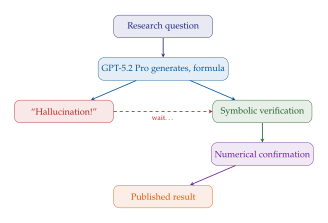
The Physics: Symmetry
The result has deep physical significance. It connects to the symmetry that Roger Penrose identified in classical gravity fifty years ago.
Theorem 16 (Graviton Extension).
The single-minus graviton amplitude in the decay kinematics region simplifies to an -fold product of soft factors: where is the soft graviton factor for particle .
Insight.
This is the first time the symmetry has been shown to act directly on graviton scattering amplitudes. The connection was entirely unexpected: the AI bridged a gap between combinatorics (the matrix-tree theorem) and quantum gravity (the algebra) that human physicists had not seen.
Hallucination as Discovery
The graviton story forces us to reconsider the relationship between hallucination and creativity.
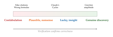
Key Idea.
The boundary between hallucination and creativity is not internal to the model but determined by external verification. A formula that fails verification is a hallucination; the same formula, if verified, is a discovery. This makes mathematics uniquely suited to AI creativity: unlike art or literature, mathematical correctness is objective.
Remark 45.
This observation has a profound implication for AI safety: formal verification systems like Lean 4 serve as a “creativity filter,” allowing AI to explore freely while catching errors before they propagate. The graviton discovery suggests that the most valuable AI contributions may come from outputs that initially look wrong.
Exercises
Exercise 105.
State the directed matrix-tree theorem for a complete graph and explain why it counts spanning trees.
Exercise 106.
Verify the single-minus gluon amplitude formula (Theorem 15) for by direct computation. How many directed spanning trees does have?
Exercise 107.
(Essay.) Compare the graviton discovery with Ramanujan's formulas for , which were also initially dismissed as “too good to be true” before being verified. What does this comparison suggest about the nature of mathematical intuition?
Exercise 108.
(Challenge.) The Parke–Taylor formula (Theorem 14) involves spinor brackets . Define these brackets in terms of the momenta and verify that .
Exercise 109.
Discuss the ethical implications of listing an AI model as a contributing author on a physics paper. Should GPT-5.2 Pro be credited as an author of the graviton paper? Why or why not?
Towards Autonomous Mathematical Research
The ultimate aspiration of AI for mathematics is not merely to solve problems posed by humans but to discover new mathematics autonomously: identifying interesting questions, developing novel proof strategies, and producing results that advance mathematical knowledge. In early 2026, the first credible steps towards this goal were taken.
The MRAL Framework Revisited
Recall from The MRAL Framework the Mathematical Research Autonomy Levels framework. Here we examine how actual systems map onto this framework.
Example 49 (Mapping Recent Achievements to MRAL).
| Achievement | Autonomy | Significance |
| GPT-4 solving AIME problems | H | 0 |
| Erdos #728 (Barreto + AI) | C | 1 |
| AlphaProof IMO 2024 | C | 1 |
| Axiom Putnam 12/12 | A | 1 |
| Aletheia Feng26 paper | A | 1 |
| LeeSeo26 (DeepMind collab.) | C | 2 |
| Graviton amplitude | C | 2–3 |
Aletheia: Fully Autonomous Research
DeepMind's Aletheia system, powered by Gemini Deep Think (January 2026 version), produced the first fully autonomous mathematical research paper [144].
Definition 34 (Aletheia Architecture).
Aletheia is an iterative mathematical research agent with three components:
Generator: Gemini Deep Think with novel inference-time scaling extending past Olympiad-level problems.
Verifier: A combination of symbolic computation (for algebraic identities), numerical simulation (for conjectures), and Lean 4 formalisation (for proofs).
Reviser: Takes failed verification attempts and uses them to refine the approach, generating new hypotheses.
The system operates in a loop: generate verify revise, with each iteration refining the mathematical content.
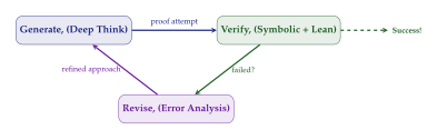
The Feng26 paper.
The paper “Feng26,” on eigenweights in arithmetic geometry, was generated with zero human intervention. The system:
Identified an open question about the distribution of eigenweights of Hecke operators on spaces of modular forms.
Formulated a precise conjecture based on numerical computation.
Developed a proof strategy using the trace formula and Selberg's method.
Produced a complete proof, verified by Lean 4 formalisation.
Generated a human-readable paper in LaTeX.
Remark 46.
Expert review classified Feng26 as a correct, publishable result at approximately the level of a good journal paper (MRAL Level A/L1). While not a major breakthrough, it represents the first credible demonstration of fully autonomous mathematical research.
The LeeSeo26 collaboration.
In contrast, the “LeeSeo26” paper, on bounds for independent sets in interacting particle systems, was a genuine human-AI collaboration (MRAL Level C/L2). Human mathematicians identified the problem and guided the high-level strategy; Aletheia contributed key technical lemmas and the formalisation.
AlphaEvolve for Mathematical Discovery
While Aletheia approaches mathematics through proof, AlphaEvolve (and its predecessor FunSearch) approaches it through search [53].
Definition 35 (Evolutionary Mathematical Discovery).
An evolutionary mathematical discovery system:
Generates candidate mathematical objects (constructions, formulas, algorithms) using an LLM.
Evaluates candidates using automated scoring functions (size, optimality, satisfaction of constraints).
Selects the best candidates and uses them to prompt the LLM for improved variants.
Iterates until convergence or resource exhaustion.
Key results from this approach:
Cap set bounds: FunSearch discovered new constructions for cap sets in , improving known lower bounds for the cap set problem [53].
Kissing numbers: AlphaEvolve found improved configurations for sphere packing in high dimensions.
Algorithm discovery: New matrix multiplication algorithms and sorting networks.
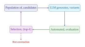
Insight.
The evolutionary approach to mathematical discovery is complementary to proof-based approaches. While Aletheia proves existing conjectures, AlphaEvolve discovers new mathematical objects. The combination of both capabilities, discovery and proof, is what a fully autonomous mathematical research system would require.
The Ramanujan Machine
The Ramanujan Machine, developed at the Technion, uses a different paradigm: massively parallel search for continued fraction formulas involving fundamental constants [148].
Example 50 (Discovered Continued Fractions).
The system discovered new continued fraction representations for:
: using , .
: using , .
: using , .
Apéry's constant : new representations connecting to the irrationality proof.
Key Idea.
In 2024, the Ramanujan Machine team published the discovery of conservative matrix fields in PNAS [54], a novel mathematical structure that unifies thousands of existing formulas and generates infinitely many new ones. These fields reveal unexpected relationships among fundamental constants and provide new pathways for irrationality proofs.
Verification and Trust
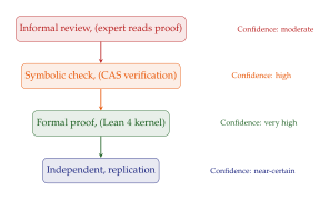
Caution.
The evaluation gap between AI company claims and mathematical standards remains significant. Press releases may announce that an AI “solved” a problem, but rigorous verification requires formal proof or extensive expert review. The MRAL framework helps calibrate expectations by separating autonomy from significance.
Exercises
Exercise 110.
Describe the generate-verify-revise loop of Aletheia and compare it with the edit-compile-debug loop in software engineering.
Exercise 111.
The Ramanujan Machine discovered formulas by brute-force search. Estimate the computational complexity of searching for continued fractions of depth with integer coefficients bounded by .
Exercise 112.
(Challenge.) Design an automated scoring function for evaluating the “interestingness” of a mathematical conjecture. What criteria would you use? How would you avoid bias towards trivially true or trivially false statements?
Exercise 113.
(Research.) The cap set problem asks for the maximum size of a subset of containing no three-term arithmetic progression. Explain why FunSearch's evolutionary approach is well-suited to this problem. What is the scoring function?
AI Conjecture Generation
Perhaps even more important than proving theorems is asking the right questions. The history of mathematics is shaped not only by proofs but by conjectures: the Riemann Hypothesis, the Poincaré Conjecture, Fermat's Last Theorem. Can AI learn to conjecture?
The Art of Conjecture
Definition 36 (Mathematical Conjecture).
A mathematical conjecture is a statement believed to be true based on evidence (computational, heuristic, or analogical) but not yet proved. A good conjecture is:
Precise: stated formally enough to be proved or disproved.
Plausible: supported by computational evidence or theoretical reasoning.
Interesting: connected to existing theory and likely to yield new insights.
Accessible: at the boundary of current knowledge, neither too easy nor impossibly hard.
Historical Note.
Srinivasa Ramanujan (1887–1920) is the archetypal mathematical conjecturer. Working largely in isolation in India, he produced thousands of formulas, many unproved. Decades later, mathematicians verified most and found them profoundly connected to deep areas of mathematics (modular forms, -series, partition theory). Ramanujan's “intuition” was not random: it reflected deep pattern recognition in mathematical structures.
AI Scanning the Mathematical Literature
A direct approach to conjecture generation is mining the existing mathematical literature for patterns.
Example 51 (Discovering Connections Among Formulas).
Researchers used LLMs to harvest expressions for from hundreds of thousands of arXiv papers. The analysis identified hundreds of unique expressions and discovered 75 previously unknown connections spanning different papers, methods, and centuries. Some connections linked apparently unrelated areas: a result in analytic number theory was equivalent to a formula derived from quantum field theory.
Self-Play Conjecture Generation
A more sophisticated approach uses dual agents in an iterative loop:
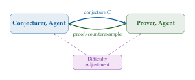
Key Idea.
The self-play loop creates a self-improving cycle: the conjecturer learns to produce statements that are challenging but provable, while the prover becomes stronger by tackling increasingly difficult conjectures. This mirrors the historical development of mathematics, where conjectures and proofs co-evolve.
The Role of Evolution
AlphaEvolve and FunSearch use evolutionary search to discover mathematical objects, which can be viewed as implicit conjecture generation:
Remark 47.
When FunSearch discovers a cap set construction of size in , it implicitly conjectures that is a new lower bound. The construction itself is the proof. This “conjecture by construction” approach bypasses the traditional conjecture-then-prove pipeline and connects directly to the evolutionary AI techniques discussed in Part XV of this book.
Problem Finding vs. Problem Solving
Conjecture 3 (The AI Taste Conjecture).
Within the next decade, AI systems will develop “mathematical taste”: the ability to distinguish important problems from trivial ones, currently a uniquely human capability.
Remark 48.
Mathematical taste is difficult to formalise. What makes the Riemann Hypothesis “important” but a random statement about large numbers “uninteresting”? Importance is connected to: (1) connections to other areas, (2) depth of technique required, (3) beauty and simplicity of statement, and (4) consequences for applications. Training an AI to recognise these properties is an open challenge.
The Future: Fully Autonomous Research Pipelines
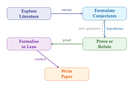
Caution.
Ethical considerations are significant. If AI systems produce autonomous mathematical research, questions arise about: authorship and credit, peer review of AI-generated papers, the value of human mathematical understanding, and the potential for flooding journals with machine-generated results of marginal significance.
Exercises
Exercise 114.
Design a “conjecture difficulty” metric that predicts how hard a conjecture will be to prove. What features would you include?
Exercise 115.
Explain why the self-play loop (Figure 81) is analogous to the generator-discriminator dynamic in GANs.
Exercise 116.
(Essay.) Is it possible for an AI to develop “mathematical taste”? Argue for or against, drawing on the nature of aesthetic judgement in mathematics.
Exercise 117.
(Research.) Propose a training objective for a “mathematical taste” model. Your model should take a mathematical statement as input and output a score predicting its importance. What training data would you use?
Connections and Synthesis
Throughout this chapter we have encountered a remarkable diversity of approaches: formal theorem provers, neural tactic generators, reinforcement learning agents, evolutionary search systems, and large language models. In this section we step back and examine how these approaches relate to each other and to the broader landscape of generative modelling.
The Grand Picture
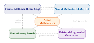
Key Idea.
The most powerful mathematical AI systems are hybrids that combine multiple paradigms. AlphaProof combines neural networks (generation) with RL (search) and Lean (verification). Aletheia combines LLMs (reasoning) with retrieval (literature search) and symbolic computation (verification). The trend is towards systems that integrate all four pillars.
Connections to Other Chapters
This chapter connects deeply to several other parts of the book:
Retrieval (Part XVI): ReProver and LeanDojo use retrieval-augmented generation to find relevant premises from Mathlib. The techniques from dense retrieval, ANN search, and embedding models directly apply.
Structured data (Part XVII): Graph-based representations of proofs, dependency structures in Mathlib, and the algebraic typeclass hierarchy are all structured data problems.
Evolutionary AI (Part XV): AlphaEvolve and FunSearch directly apply evolutionary search to mathematical discovery. The co-evolutionary dynamics between conjecturers and provers mirror competitive coevolution.
RL and alignment (Part IX): GRPO, PPO, and expert iteration for theorem proving are instances of RLHF with the Lean compiler as the “human” providing feedback.
Reasoning (Part VII): Chain-of-thought, tree-of-thought, and recursive reasoning are foundational to mathematical AI.
The Verification Advantage
Theorem 17 (The Verification Advantage, Informal).
Mathematics is uniquely suited to AI among intellectual domains because mathematical correctness is decidable for any given proof: given a complete formal proof in a system like Lean 4, a finite computation determines whether it is valid.
Remark 49.
This stands in contrast to:
Natural language: There is no objective “truth verifier” for an essay or a novel.
Science: Experimental verification requires physical resources and may not be reproducible.
Engineering: Real-world testing involves uncertainty, approximation, and physical constraints.
Code: While unit tests provide partial verification, proving correctness of arbitrary programs is undecidable in general.
The decidability of proof verification means that mathematical AI can be given a perfect reward signal, making RL for mathematics fundamentally different from RL for other domains.
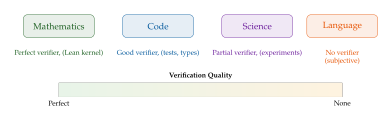
Comparison with AlphaFold
| Dimension | AlphaFold | Mathematical AI |
| Output | 3D coordinates | Proof (logical chain) |
| Verification | Empirical (X-ray) | Formal (Lean kernel) |
| Training data | 200K structures | Millions of proofs |
| Correctness | Continuous confidence | Binary (correct/incorrect) |
| Human parity | Surpassed most experts | Approaching graduate level |
| Generalisation | Struggles with novel folds | Struggles with novel techniques |
Historical Timeline and Open Problems
Timeline
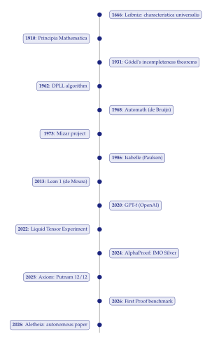
Open Problems
We organise the open problems into four categories.
Theoretical.
Can transformers learn to prove? What is the computational complexity of proof search in the transformer architecture?
What is the sample complexity of RL for theorem proving? How many proofs must a model see to generalise to new theorems?
Is there a theoretical limit to autoformalization accuracy? Can we prove impossibility results?
Practical.
How do we scale formal libraries beyond Mathlib? Can we formalise all of undergraduate mathematics? All of research mathematics?
What is the cost-optimal architecture for theorem proving? How do we balance model size, search budget, and verification overhead?
Can we build universal autoformalisers that work across mathematical domains?
Philosophical.
What constitutes mathematical “understanding”? Does a model that proves a theorem “understand” it in any meaningful sense?
Can AI be genuinely creative in mathematics, or only recombinative? Is there a principled distinction?
The Chinese Room argument for proofs: if a system produces valid proofs by manipulating symbols without “understanding” the mathematics, does this diminish the value of the proofs?
Grand Challenges.
Solve a Millennium Prize problem with AI assistance.
Achieve consistent IMO Gold (all 6 problems) autonomously.
Produce Level A/L4 mathematical research: a transformative result generated entirely by AI.
Build a self-improving mathematical research system that discovers new subfields.
Exercises and Research Challenges
We conclude with a comprehensive collection of exercises at multiple difficulty levels.
Introductory Exercises
Exercise 118.
Explain the Curry–Howard correspondence in your own words. Give three examples of logical connectives and their type-theoretic counterparts.
Exercise 119.
What is proof irrelevance and why is it important for mathematical formalisation? Give an example where it matters.
Exercise 120.
List five tactics in Lean 4 and explain when each is most useful.
Exercise 121.
Explain the difference between simp and ring in
Lean 4. When would you use one over the other?
Intermediate Exercises
Exercise 122.
Compare and contrast the approaches of AlphaProof (RL + Lean), Aristotle (expert iteration + geometry), and Axiom/AXLE (pipeline with auto-formalization). Which approach is most likely to scale to harder problems? Justify your answer.
Exercise 123.
Derive the GRPO advantage estimator from first principles. Show that it is unbiased and explain the role of the group size .
Exercise 124.
The MiniF2F benchmark contains 488 problems. If a system achieves 90% accuracy, how many problems does it solve? If each solved problem requires on average 50 tactic steps, and each step takes 100ms to generate, estimate the total computation time.
Exercise 125.
Explain why MCTS is well-suited to proof search. What corresponds to the “game state,” “legal moves,” and “terminal reward” in the proof search analogy?
Advanced Exercises
Exercise 126.
(Lean Programming.) Prove in Lean 4 that the composition of two injective functions is injective. Provide the complete code.
Exercise 127.
(Lean Programming.) Formalise the statement “every finite group of prime order is cyclic” in Lean 4. You may use Mathlib. Identify the key lemmas needed.
Exercise 128.
(RL Design.) Design an RL training loop for a Lean 4 tactic generator. Specify: the state space, action space, reward function, and training algorithm. How would you handle the sparse reward problem?
Exercise 129.
(Architecture Design.) Design a retrieval-augmented tactic generator. Given a proof state, how would you retrieve relevant premises from Mathlib? What embedding model would you use? How would you combine retrieval with generation?
Research Challenges
Challenge 3.
The Autoformalization Challenge. Select five theorems from a real analysis textbook that are not in Mathlib. Formalise them in Lean 4, documenting the difficulties encountered. Estimate the effort required to automate this process and identify the main bottlenecks.
Challenge 4.
The Conjecture Generation Challenge. Build a system that generates mathematical conjectures about sequences in the OEIS (Online Encyclopedia of Integer Sequences). Your system should: (a) select a sequence, (b) generate a conjecture about its growth rate or algebraic properties, (c) test the conjecture computationally, and (d) attempt a proof or find a counterexample.
Challenge 5.
The Benchmark Design Challenge. Design a mathematical AI benchmark that fills the gap between MATH (competition level) and FrontierMath (research level). Your benchmark should target the level of a first-year graduate course. Specify the domains, difficulty criteria, evaluation protocol, and anti-contamination measures.
Challenge 6.
The Self-Play Mathematics Challenge. Implement a self-play loop for mathematical conjecture generation and proving. Use a language model as both conjecturer and prover, with a formal verifier (Lean 4 or a simpler system) providing the reward signal. Measure whether the quality of conjectures improves over training iterations.
Challenge 7.
The Verification Pipeline Challenge. Build an end-to-end pipeline that takes a natural-language mathematical proof (e.g., from a textbook or arXiv paper) and produces a verified Lean 4 formalisation. Measure the success rate on a set of undergraduate-level proofs and analyse the failure modes.
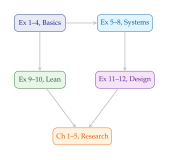
References
-
MaLARea SG1 -- Machine Learner for Automated Reasoning with Semantic Guidance
BibTeX
@inproceedings{urban2011malarea, title={{MaLARea SG1} -- Machine Learner for Automated Reasoning with Semantic Guidance}, author={Urban, Josef and Vyskoil, Ji{\v{r}}{\'\i} and {\v{S}}t{\v{e}}p{\'a}nek, Petr}, booktitle={International Joint Conference on Automated Reasoning (IJCAR)}, year={2011}, publisher={Springer} }Conference paper
-
Generative Language Modeling for Automated Theorem Proving
BibTeX
@article{polu2020generative, title = {Generative Language Modeling for Automated Theorem Proving}, author = {Polu, Stanislas and Sutskever, Ilya}, journal = {arXiv preprint arXiv:2009.03393}, year = {2020} }Journal article
-
Solving olympiad geometry without human demonstrations
BibTeX
@article{deepmind2024alphageometry, title = {Solving olympiad geometry without human demonstrations}, author = {Trinh, Trieu H. and Wu, Yuhuai and Le, Quoc V. and He, He and Luong, Thang}, journal = {Nature}, volume = {625}, pages = {476--482}, year = {2024} }Journal article
-
DeepSeek-Prover-V1.5: Harnessing Proof Assistant Feedback for Reinforcement Learning and Monte-Carlo Tree Search
BibTeX
@article{xin2024deepseekprover, title = {{DeepSeek-Prover-V1.5}: Harnessing Proof Assistant Feedback for Reinforcement Learning and Monte-Carlo Tree Search}, author = {Xin, Huajian and others}, journal = {arXiv preprint arXiv:2408.08152}, year = {2024} }Journal article
-
Four Colors Suffice: How the Map Problem Was Solved
BibTeX
@book{wilson2013four, title={Four Colors Suffice: How the Map Problem Was Solved}, author={Wilson, Robin}, year={2013}, publisher={Princeton University Press}, edition={Revised Color Edition} }Book
-
Modular Elliptic Curves and Fermat's Last Theorem
BibTeX
@article{wiles1995modular, title={Modular Elliptic Curves and {Fermat's Last Theorem}}, author={Wiles, Andrew}, journal={Annals of Mathematics}, volume={141}, number={3}, pages={443--551}, year={1995} }Journal article
-
A Formal Proof of the Kepler Conjecture
BibTeX
@article{hales2017formal, title={A Formal Proof of the {Kepler} Conjecture}, author={Hales, Thomas C. and Adams, Mark and Bauer, Gertrud and Dang, Tat Dat and Harrison, John and Hoang, Le Truong and Kaliszyk, Cezary and Magron, Victor and McLaughlin, Sean and Nguyen, Tat Thang and others}, journal={Forum of Mathematics, Pi}, volume={5}, year={2017}, publisher={Cambridge University Press} }Journal article
-
Proof Artifact Co-Training for Theorem Proving with Language Models
BibTeX
@inproceedings{han2022proof, title={Proof Artifact Co-Training for Theorem Proving with Language Models}, author={Han, Jesse Michael and Rute, Jason and Wu, Yuhuai and Ayers, Edward W. and Bansal, Siddhartha}, booktitle={International Conference on Learning Representations (ICLR)}, year={2022} }Conference paper
-
LeanDojo-v2
BibTeX
@article{yang2024leandojo, title = {{LeanDojo}-v2}, author = {Yang, Kaiyu and others}, journal = {arXiv preprint}, year = {2024} }Journal article
-
Solving Quantitative Reasoning Problems with Language Models
BibTeX
@misc{lewkowycz2022solving, title = {Solving Quantitative Reasoning Problems with Language Models}, author = {Lewkowycz, Aitor and others}, year = {2022} }Reference
-
Chain-of-Thought Prompting Elicits Reasoning in Large Language Models
BibTeX
@article{wei2022chain, title={Chain-of-Thought Prompting Elicits Reasoning in Large Language Models}, author={Wei, Jason and Wang, Xuezhi and Schuurmans, Dale and Bosma, Maarten and Ichter, Brian and Xia, Fei and Chi, Ed and Le, Quoc and Zhou, Denny}, journal={Advances in Neural Information Processing Systems}, volume={35}, pages={24824--24837}, year={2022} }Journal article
-
The Lean Theorem Prover (System Description)
BibTeX
@inproceedings{demoura2015lean, author = {de Moura, Leonardo and Kong, Soonho and Avigad, Jeremy and van Doorn, Floris and von Raumer, Jakob}, title = {The {Lean} Theorem Prover (System Description)}, booktitle = {International Conference on Automated Deduction}, pages = {378--388}, year = {2015} }Conference paper
-
The Lean 4 Theorem Prover and Programming Language
BibTeX
@misc{moura2021lean4, title = {The Lean 4 Theorem Prover and Programming Language}, author = {de Moura, Leonardo and Ullrich, Sebastian}, year = {2021}, note = {CADE-28} }Reference
-
Mathlib: The Lean Mathematical Library
BibTeX
@misc{mathlib2024, title={Mathlib: The {Lean} Mathematical Library}, author={{Mathlib Community}}, year={2024}, note={\url{https://leanprover-community.github.io/mathlib4_docs/}} }Reference
-
Formal Proof -- The Four-Color Theorem
BibTeX
@article{gonthier2008four, title={Formal Proof -- The Four-Color Theorem}, author={Gonthier, Georges}, journal={Notices of the American Mathematical Society}, volume={55}, number={11}, pages={1382--1393}, year={2008} }Journal article
-
A Machine-Checked Proof of the Odd Order Theorem
BibTeX
@article{gonthier2013oddorder, title = {A Machine-Checked Proof of the Odd Order Theorem}, author = {Gonthier, Georges and others}, journal = {ITP 2013}, year = {2013} }Journal article
-
Formal Certification of a Compiler Back-end or: Programming a Compiler with a Proof Assistant
BibTeX
@inproceedings{leroy2006compcert, title={Formal Certification of a Compiler Back-end or: Programming a Compiler with a Proof Assistant}, author={Leroy, Xavier}, booktitle={ACM SIGPLAN-SIGACT Symposium on Principles of Programming Languages (POPL)}, year={2006} }Conference paper
-
Sledgehammer: Judgement Day
BibTeX
@incollection{blanchette2016sledgehammer, title={Sledgehammer: Judgement Day}, author={Blanchette, Jasmin Christian and B{\"o}hme, Sascha and Paulson, Lawrence C.}, booktitle={Automated Reasoning (IJCAR)}, year={2016}, publisher={Springer} }Book chapter
-
A Formal Proof of the Kepler Conjecture
BibTeX
@article{hales2017kepler, title={A Formal Proof of the {Kepler} Conjecture}, author={Hales, Thomas C. and Adams, Mark and Bauer, Gertrud and Dang, Tat Dat and Harrison, John and Hoang, Le Truong and Kaliszyk, Cezary and Magron, Victor and McLaughlin, Sean and Nguyen, Tat Thang and others}, journal={Forum of Mathematics, Pi}, volume={5}, year={2017}, publisher={Cambridge University Press}, note={The Flyspeck project} }Journal article
-
seL4: Formal Verification of an OS Kernel
BibTeX
@inproceedings{klein2009sel4, title={{seL4}: Formal Verification of an {OS} Kernel}, author={Klein, Gerwin and Elphinstone, Kevin and Heiser, Gernot and Andronick, June and Cock, David and Derrin, Philip and Elkaduwe, Dhammika and Engelhardt, Kai and Kolanski, Rafal and Norrish, Michael and others}, booktitle={ACM SIGOPS Symposium on Operating Systems Principles (SOSP)}, year={2009} }Conference paper
-
On the Complexity of Derivation in Propositional Calculus
BibTeX
@incollection{tseitin1983complexity, title={On the Complexity of Derivation in Propositional Calculus}, author={Tseitin, Grigori S.}, booktitle={Automation of Reasoning: 2. Classical Papers on Computational Logic 1967--1970}, pages={466--483}, year={1983}, publisher={Springer}, note={Originally published in 1968} }Book chapter
-
A Machine-Oriented Logic Based on the Resolution Principle
BibTeX
@article{robinson1965machine, title = {A Machine-Oriented Logic Based on the Resolution Principle}, author = {Robinson, John Alan}, journal = {Journal of the ACM}, volume = {12}, number = {1}, pages = {23--41}, year = {1965} }Journal article
-
First-Order Theorem Proving and Vampire
BibTeX
@inproceedings{kovacs2013firstorder, title={First-Order Theorem Proving and {Vampire}}, author={Kov{\'a}cs, Laura and Voronkov, Andrei}, booktitle={International Conference on Computer Aided Verification (CAV)}, year={2013}, publisher={Springer} }Conference paper
-
E -- A Brainiac Theorem Prover
BibTeX
@inproceedings{schulz2002eprover, title={{E} -- A Brainiac Theorem Prover}, author={Schulz, Stephan}, booktitle={AI Communications}, volume={15}, number={2--3}, pages={111--126}, year={2002} }Conference paper
-
SPASS Version 2.0
BibTeX
@inproceedings{weidenbach2001spass, title={{SPASS} Version 2.0}, author={Weidenbach, Christoph and Dimova, Dilyana and Fietzke, Arnaud and Kumar, Rohit and Suda, Martin and Wischnewski, Patrick}, booktitle={International Conference on Automated Deduction (CADE)}, year={2001}, publisher={Springer} }Conference paper
-
Z3: An Efficient SMT Solver
BibTeX
@article{demoura2008z3, title = {Z3: An Efficient {SMT} Solver}, author = {de Moura, Leonardo and Bj{\o}rner, Nikolaj}, journal = {TACAS}, year = {2008} }Journal article
-
cvc5: A Versatile and Industrial-Strength SMT Solver
BibTeX
@inproceedings{barbosa2022cvc5, title={cvc5: A Versatile and Industrial-Strength {SMT} Solver}, author={Barbosa, Haniel and Barrett, Clark and Brain, Martin and Kremer, Gereon and Lachnitt, Hanna and Mann, Makai and Mohamed, Abdalrhman and Mohamed, Mudathir and Niemetz, Aina and N{\"o}tzli, Andres and Ozdemir, Alex and Preiner, Mathias and Reynolds, Andrew and Sheng, Ying and Tinelli, Cesare and Zohar, Yoni}, booktitle={International Conference on Tools and Algorithms for the Construction and Analysis of Systems (TACAS)}, year={2022} }Conference paper
-
Yices 2.2
BibTeX
@inproceedings{dutertre2014yices, title={Yices 2.2}, author={Dutertre, Bruno}, booktitle={International Conference on Computer Aided Verification (CAV)}, year={2014}, publisher={Springer} }Conference paper
-
Dafny: An Automatic Program Verifier for Functional Correctness
BibTeX
@inproceedings{leino2010dafny, title={{Dafny}: An Automatic Program Verifier for Functional Correctness}, author={Leino, K. Rustan M.}, booktitle={International Conference on Logic for Programming, Artificial Intelligence, and Reasoning (LPAR)}, year={2010}, publisher={Springer} }Conference paper
-
KLEE: Unassisted and Automatic Generation of High-Coverage Tests for Complex Systems Programs
BibTeX
@inproceedings{cadar2008klee, title={{KLEE}: Unassisted and Automatic Generation of High-Coverage Tests for Complex Systems Programs}, author={Cadar, Cristian and Dunbar, Daniel and Engler, Dawson}, booktitle={USENIX Symposium on Operating Systems Design and Implementation (OSDI)}, year={2008} }Conference paper
-
MaSh: Machine Learning for Sledgehammer
BibTeX
@inproceedings{kuhlwein2013mash, title={{MaSh}: Machine Learning for {Sledgehammer}}, author={K{\"u}hlwein, Daniel and Blanchette, Jasmin Christian and Kaliszyk, Cezary and Urban, Josef}, booktitle={International Conference on Interactive Theorem Proving (ITP)}, year={2013}, publisher={Springer} }Conference paper
-
Every Planar Map is Four Colorable
BibTeX
@article{appel1977fourcolor, title={Every Planar Map is Four Colorable}, author={Appel, Kenneth and Haken, Wolfgang}, journal={Bulletin of the American Mathematical Society}, volume={82}, number={5}, pages={711--712}, year={1977} }Journal article
merrill2023expresssive
-
Towards Revealing the Mystery behind Chain of Thought: A Theoretical Perspective
BibTeX
@article{feng2023towards, title={Towards Revealing the Mystery behind Chain of Thought: A Theoretical Perspective}, author={Feng, Guhao and Zhang, Bohang and Gu, Yuntian and Ye, Haotian and He, Di and Wang, Liwei}, journal={Advances in Neural Information Processing Systems}, volume={36}, year={2023} }Journal article
-
Let's Verify Step by Step
BibTeX
@article{lightman2023verify, title={Let's Verify Step by Step}, author={Lightman, Hunter and Kosaraju, Vineet and Burda, Yura and Edwards, Harri and Baker, Bowen and Lee, Teddy and Leike, Jan and Schulman, John and Sutskever, Ilya and Cobbe, Karl}, journal={arXiv preprint arXiv:2305.20050}, year={2023} }Journal article
-
Thinking, Fast and Slow
BibTeX
@book{kahneman2011thinking, title={Thinking, Fast and Slow}, author={Kahneman, Daniel}, year={2011}, publisher={Farrar, Straus and Giroux} }Book
-
Llemma: An Open Language Model for Mathematics
BibTeX
@inproceedings{azerbayev2024llemma, title={Llemma: An Open Language Model for Mathematics}, author={Azerbayev, Zhangir and Schoelkopf, Hailey and Paster, Keiran and Dos Santos, Marco and McAleer, Stephen and Jiang, Albert Q. and Deng, Jia and Biderman, Stella and Welleck, Sean}, booktitle={International Conference on Learning Representations (ICLR)}, year={2024} }Conference paper
-
InternLM-Math: Open Math Large Language Models Toward Verifiable Reasoning
BibTeX
@article{ying2024internlmmath, title={{InternLM-Math}: Open Math Large Language Models Toward Verifiable Reasoning}, author={Ying, Huaiyuan and Zhang, Shuo and Li, Linyang and Zhou, Zhejian and Shao, Yunfan and Fei, Zhaoye and Ma, Yichuan and Hong, Jiawei and Liu, Kuikun and Wang, Ziyi and others}, journal={arXiv preprint arXiv:2402.06332}, year={2024} }Journal article
-
Qwen2.5-Math Technical Report: Toward Mathematical Expert Model via Self-Improvement
BibTeX
@article{yang2024qwen25math, title={{Qwen2.5-Math} Technical Report: Toward Mathematical Expert Model via Self-Improvement}, author={Yang, An and Yang, Beichen and Hui, Binyuan and Zheng, Bo and Yu, Bowen and Zhou, Chang and others}, journal={arXiv preprint arXiv:2409.12122}, year={2024} }Journal article
-
Principia Mathematica (2nd ed.)
BibTeX
@misc{whitehead1925principia, title = {Principia Mathematica (2nd ed.)}, author = {Whitehead, Alfred North and Russell, Bertrand}, year = {1925} }Reference
-
Uber formal unentscheidbare Satze der Principia Mathematica und verwandter Systeme I
BibTeX
@article{godel1931formal, title = {{\"U}ber formal unentscheidbare {S}{\"a}tze der {P}rincipia {M}athematica und verwandter {S}ysteme {I}}, author = {G{\"o}del, Kurt}, journal = {Monatshefte f{\"u}r Mathematik und Physik}, volume = {38}, pages = {173--198}, year = {1931} }Journal article
-
The QED Manifesto
BibTeX
@inproceedings{boyer1994qed, title={The {QED} Manifesto}, author={Boyer, Robert S. and others}, booktitle={Automated Deduction -- CADE-12}, year={1994}, publisher={Springer} }Conference paper
-
Mastering the game of Go with deep neural networks and tree search
BibTeX
@article{silver2016mastering, title = {Mastering the game of {Go} with deep neural networks and tree search}, author = {Silver, David and Huang, Aja and Maddison, Chris J. and Guez, Arthur and Sifre, Laurent and others}, journal = {Nature}, volume = {529}, pages = {484--489}, year = {2016} }Journal article
-
Representation Learning with Contrastive Predictive Coding
BibTeX
@article{oord2018representation, author = {Oord, Aaron van den and Li, Yazhe and Vinyals, Oriol}, title = {Representation Learning with Contrastive Predictive Coding}, journal = {arXiv preprint arXiv:1807.03748}, year = {2018} }Journal article
-
Four Colors Suffice: How the Map Problem Was Solved
BibTeX
@book{wilson2019sixty, title={Four Colors Suffice: How the Map Problem Was Solved}, author={Wilson, Robin}, year={2014}, publisher={Princeton University Press}, note={Includes historical survey of sixty years of work on the four-color problem} }Book
-
AlphaProof: AI achieves silver-medal standard solving International Mathematical Olympiad problems
BibTeX
@article{deepmind2024alphaproof, title = {{AlphaProof}: {AI} achieves silver-medal standard solving International Mathematical Olympiad problems}, author = {{Google DeepMind}}, journal = {Nature}, year = {2025}, note = {doi:10.1038/s41586-025-09833-y} }Journal article
-
Solving Olympiad Geometry without Human Demonstrations
BibTeX
@article{trinh2024solving, title={Solving Olympiad Geometry without Human Demonstrations}, author={Trinh, Trieu H. and Wu, Yuhuai and Le, Quoc V. and He, He and Luong, Thang}, journal={Nature}, volume={625}, number={7995}, pages={476--482}, year={2024} }Journal article
-
Discovering Faster Matrix Multiplication Algorithms with Reinforcement Learning
BibTeX
@article{fawzi2022discovering, title={Discovering Faster Matrix Multiplication Algorithms with Reinforcement Learning}, author={Fawzi, Alhussein and Balog, Matej and Huang, Aja and Hubert, Thomas and Romera-Paredes, Bernardino and Barekatain, Mohammadamin and Novikov, Alexander and Ruiz, Francisco J. R. and Schrittwieser, Julian and Swirszcz, Grzegorz and others}, journal={Nature}, volume={610}, number={7930}, pages={47--53}, year={2022} }Journal article
-
DeepSeek-R1: Incentivizing Reasoning Capability in LLMs via Reinforcement Learning
BibTeX
@article{deepseek2025r1, title = {{DeepSeek-R1}: Incentivizing Reasoning Capability in {LLMs} via Reinforcement Learning}, author = {{DeepSeek AI}}, journal = {arXiv preprint arXiv:2501.12948}, year = {2025} }Journal article
-
FrontierMath: A Benchmark for Evaluating Advanced Mathematical Reasoning in AI
BibTeX
@misc{glazer2024frontiermath, title = {{FrontierMath}: A Benchmark for Evaluating Advanced Mathematical Reasoning in {AI}}, author = {Glazer, Elliot and others}, year = {2024}, note = {epoch.ai/frontiermath} }Reference
-
DeepSeekMath: Pushing the Limits of Mathematical Reasoning in Open Language Models
BibTeX
@article{shao2024deepseekmath, title={{DeepSeekMath}: Pushing the Limits of Mathematical Reasoning in Open Language Models}, author={Shao, Zhihong and Wang, Peiyi and Zhu, Qihao and Xu, Runxin and Song, Junxiao and Zhang, Mingchuan and Li, Y.K. and Wu, Y. and Guo, Daya}, journal={arXiv preprint arXiv:2402.03300}, year={2024} }Journal article
-
Axiom: Quantitative Super-Intelligence for Mathematics
BibTeX
@misc{axiommath2025, title = {Axiom: Quantitative Super-Intelligence for Mathematics}, author = {{Axiom Math}}, year = {2025}, note = {axiommath.ai} }Reference
-
Mathematical Discoveries from Program Search with Large Language Models
BibTeX
@article{romera2024funsearch, author = {Romera-Paredes, Bernardino and others}, title = {Mathematical Discoveries from Program Search with Large Language Models}, journal = {Nature}, volume = {625}, pages = {468--475}, year = {2024} }Journal article
-
Conservative matrix fields and the Ramanujan machine
BibTeX
@article{cmf2024, title = {Conservative matrix fields and the {Ramanujan} machine}, author = {Raayoni, Gal and others}, journal = {Proceedings of the National Academy of Sciences}, year = {2024} }Journal article
-
Evaluating Large Language Models Trained on Code
BibTeX
@article{chen2021evaluating, title={Evaluating Large Language Models Trained on Code}, author={Chen, Mark and Tworek, Jerry and Jun, Heewoo and Yuan, Qiming and Pinto, Henrique Ponde de Oliveira and Kaplan, Jared and Edwards, Harri and Burda, Yura and Joseph, Nicholas and Brockman, Greg and others}, journal={arXiv preprint arXiv:2107.03374}, year={2021} }Journal article
-
Training Language Models to Follow Instructions with Human Feedback
BibTeX
@article{ouyang2022training, title={Training Language Models to Follow Instructions with Human Feedback}, author={Ouyang, Long and Wu, Jeffrey and Jiang, Xu and Almeida, Diogo and Wainwright, Carroll and Mishkin, Pamela and Zhang, Chong and Agarwal, Sandhini and Slama, Katarina and Ray, Alex and others}, journal={Advances in Neural Information Processing Systems}, volume={35}, pages={27730--27744}, year={2022} }Journal article
-
The Logic Theory Machine: A Complex Information Processing System
BibTeX
@inproceedings{newell1956logic, title={The Logic Theory Machine: A Complex Information Processing System}, author={Newell, Allen and Simon, Herbert A.}, booktitle={IRE Transactions on Information Theory}, volume={2}, number={3}, pages={61--79}, year={1956} }Conference paper
-
Principia Mathematica
BibTeX
@book{whitehead1910principia, title = {Principia Mathematica}, author = {Whitehead, Alfred North and Russell, Bertrand}, publisher = {Cambridge University Press}, year = {1910} }Book
-
The Mathematical Language AUTOMATH, Its Usage, and Some of Its Extensions
BibTeX
@incollection{debruijn1968automath, title={The Mathematical Language {AUTOMATH}, Its Usage, and Some of Its Extensions}, author={de Bruijn, Nicolaas Govert}, booktitle={Symposium on Automatic Demonstration}, pages={29--61}, year={1970}, publisher={Springer} }Book chapter
-
Mizar in a Nutshell
BibTeX
@article{grabowski2010mizar, title={Mizar in a Nutshell}, author={Grabowski, Adam and Korni{\l}owicz, Artur and Naumowicz, Adam}, journal={Journal of Formalized Reasoning}, volume={3}, number={2}, pages={153--245}, year={2010} }Journal article
-
Interactive Theorem Proving and Program Development: Coq'Art
BibTeX
@book{bertot2004interactive, title = {Interactive Theorem Proving and Program Development: Coq'Art}, author = {Bertot, Yves and Cast{\'e}ran, Pierre}, publisher = {Springer}, year = {2004} }Book
-
Formal Proof -- The Four-Color Theorem
BibTeX
@inproceedings{gonthier2008formal, title = {Formal Proof -- The Four-Color Theorem}, author = {Gonthier, Georges}, booktitle = {Notices of the AMS}, volume = {55}, number = {11}, pages = {1382--1393}, year = {2008} }Conference paper
-
A Machine-Checked Proof of the Odd Order Theorem
BibTeX
@inproceedings{gonthier2013machine, title={A Machine-Checked Proof of the Odd Order Theorem}, author={Gonthier, Georges and Asperti, Andrea and Avigad, Jeremy and Bertot, Yves and Cohen, Cyril and Garillot, Fran{\c{c}}ois and Le Roux, St{\'e}phane and Mahboubi, Assia and O'Connor, Russell and Ould Biha, Sidi and others}, booktitle={International Conference on Interactive Theorem Proving (ITP)}, year={2013}, publisher={Springer} }Conference paper
-
Isabelle/HOL: A Proof Assistant for Higher-Order Logic
BibTeX
@book{nipkow2002isabelle, title = {Isabelle/{HOL}: A Proof Assistant for Higher-Order Logic}, author = {Nipkow, Tobias and Paulson, Lawrence C. and Wenzel, Markus}, publisher = {Springer}, year = {2002} }Book
-
Hammering towards QED
BibTeX
@article{blanchette2016hammering, title={Hammering towards {QED}}, author={Blanchette, Jasmin Christian and Kaliszyk, Cezary and Paulson, Lawrence C. and Urban, Josef}, journal={Journal of Formalized Reasoning}, volume={9}, number={1}, pages={101--148}, year={2016} }Journal article
-
The Lean 4 Theorem Prover and Programming Language
BibTeX
@inproceedings{demoura2021lean4, title={The {Lean 4} Theorem Prover and Programming Language}, author={de Moura, Leonardo and Ullrich, Sebastian}, booktitle={International Conference on Automated Deduction (CADE)}, year={2021}, publisher={Springer} }Conference paper
-
The Lean Mathematical Library
BibTeX
@article{mathlib2020, title = {The Lean Mathematical Library}, author = {{The mathlib Community}}, journal = {CPP 2020}, year = {2020} }Journal article
-
The Design and Implementation of VAMPIRE
BibTeX
@inproceedings{riazanov2002design, title={The Design and Implementation of {VAMPIRE}}, author={Riazanov, Alexandre and Voronkov, Andrei}, booktitle={AI Communications}, volume={15}, number={2--3}, pages={91--110}, year={2002} }Conference paper
-
E -- A Brainiac Theorem Prover
BibTeX
@inproceedings{schulz2002brainiac, title={{E} -- A Brainiac Theorem Prover}, author={Schulz, Stephan}, booktitle={AI Communications}, volume={15}, number={2--3}, pages={111--126}, year={2002} }Conference paper
-
Solving and Verifying the Boolean Pythagorean Triples Problem via Cube-and-Conquer
BibTeX
@inproceedings{heule2016schur, title={Solving and Verifying the {Boolean} {Pythagorean} Triples Problem via Cube-and-Conquer}, author={Heule, Marijn J. H. and Kullmann, Oliver and Marek, Victor W.}, booktitle={International Conference on Theory and Applications of Satisfiability Testing (SAT)}, year={2016}, publisher={Springer} }Conference paper
-
Machine Learning of Coq Proof Guidance: First Experiments
BibTeX
@inproceedings{kaliszyk2014machine, title={Machine Learning of {Coq} Proof Guidance: First Experiments}, author={Kaliszyk, Cezary and Urban, Josef}, booktitle={International Symposium on Symbolic and Numeric Algorithms for Scientific Computing (SYNASC)}, year={2014} }Conference paper
-
GPT-4 Technical Report
BibTeX
@article{openai2023gpt4, title={{GPT-4} Technical Report}, author={{OpenAI}}, journal={arXiv preprint arXiv:2303.08774}, year={2023} }Journal article
-
Let's Verify Step by Step
BibTeX
@article{lightman2024lets, title={Let's Verify Step by Step}, author={Lightman, Hunter and Kosaraju, Vineet and Burda, Yura and Edwards, Harri and Baker, Bowen and Lee, Teddy and Leike, Jan and Schulman, John and Sutskever, Ilya and Cobbe, Karl}, journal={arXiv preprint arXiv:2305.20050}, year={2024}, note={Published at ICLR 2024} }Journal article
-
A Promising Path Towards Autoformalization and General Artificial Intelligence
BibTeX
@article{szegedy2020promising, title={A Promising Path Towards Autoformalization and General Artificial Intelligence}, author={Szegedy, Christian}, journal={arXiv preprint arXiv:2004.12868}, year={2020} }Journal article
-
Autoformalization with Large Language Models
BibTeX
@article{wu2022autoformalization, title={Autoformalization with Large Language Models}, author={Wu, Yuhuai and Jiang, Albert Q. and Li, Wenda and Rabe, Markus and Staats, Charles and Jamnik, Mateja and Szegedy, Christian}, journal={Advances in Neural Information Processing Systems (NeurIPS)}, year={2022} }Journal article
-
The Omega Test: A Fast and Practical Integer Programming Algorithm for Dependence Analysis
BibTeX
@inproceedings{pugh1991omega, title={The {Omega} Test: A Fast and Practical Integer Programming Algorithm for Dependence Analysis}, author={Pugh, William}, booktitle={ACM/IEEE Conference on Supercomputing}, year={1991} }Conference paper
-
The Coq Proof Assistant
BibTeX
@misc{coq2024, title={The {Coq} Proof Assistant}, author={{The Coq Development Team}}, year={2024}, note={\url{https://coq.inria.fr}} }Reference
-
Towards a Practical Programming Language Based on Dependent Type Theory
BibTeX
@phdthesis{norell2007agda, title={Towards a Practical Programming Language Based on Dependent Type Theory}, author={Norell, Ulf}, year={2007}, school={Chalmers University of Technology} }PhD thesis
-
Learning to Prove Theorems by Learning to Generate Theorems
BibTeX
@inproceedings{wang2020exploration, title={Learning to Prove Theorems by Learning to Generate Theorems}, author={Wang, Mingzhe and Deng, Jia}, booktitle={Advances in Neural Information Processing Systems (NeurIPS)}, year={2020} }Conference paper
-
Introduction to HOL: A Theorem Proving Environment for Higher Order Logic
BibTeX
@book{gordon1993hol, title={Introduction to {HOL}: A Theorem Proving Environment for Higher Order Logic}, author={Gordon, Michael J. C. and Melham, Tom F.}, year={1993}, publisher={Cambridge University Press} }Book
-
CakeML: A Verified Implementation of ML
BibTeX
@inproceedings{kumar2014cakeml, title={{CakeML}: A Verified Implementation of {ML}}, author={Kumar, Ramana and Myreen, Magnus O. and Norrish, Michael and Owens, Scott}, booktitle={ACM SIGPLAN-SIGACT Symposium on Principles of Programming Languages (POPL)}, year={2014} }Conference paper
-
Metamath: A Computer Language for Mathematical Proofs
BibTeX
@book{megill2019metamath, title={Metamath: A Computer Language for Mathematical Proofs}, author={Megill, Norman and Wheeler, David A.}, year={2019}, publisher={Lulu Press}, note={\url{http://us.metamath.org}} }Book
-
GPT-f: Generative Language Modeling for Automated Theorem Proving
BibTeX
@article{polu2020gptf, title = {{GPT-f}: Generative Language Modeling for Automated Theorem Proving}, author = {Polu, Stanislas and Sutskever, Ilya}, journal = {arXiv preprint arXiv:2009.03393}, year = {2020} }Journal article
-
Computer-Aided Reasoning: ACL2 Case Studies
BibTeX
@book{kaufmann2000acl2, title={Computer-Aided Reasoning: {ACL2} Case Studies}, author={Kaufmann, Matt and Manolios, Panagiotis and Moore, J Strother}, year={2000}, publisher={Kluwer Academic Publishers} }Book
-
Multilingual Mathematical Autoformalization
BibTeX
@article{jiang2023multilingual, title={Multilingual Mathematical Autoformalization}, author={Jiang, Albert Q. and Li, Wenda and Jamnik, Mateja}, journal={arXiv preprint arXiv:2311.03755}, year={2023} }Journal article
-
Unsupervised Cross-lingual Representation Learning at Scale
BibTeX
@inproceedings{conneau2020xlm, title={Unsupervised Cross-lingual Representation Learning at Scale}, author={Conneau, Alexis and Khandelwal, Kartikay and Goyal, Naman and Chaudhary, Vishrav and Wenzek, Guillaume and Guzm{\'a}n, Francisco and Grave, Edouard and Ott, Myle and Zettlemoyer, Luke and Stoyanov, Veselin}, booktitle={Proceedings of the 58th Annual Meeting of the Association for Computational Linguistics (ACL)}, pages={8440--8451}, year={2020} }Conference paper
-
Learning to Prove Theorems via Interacting with Proof Assistants
BibTeX
@inproceedings{yang2019coqgym, title={Learning to Prove Theorems via Interacting with Proof Assistants}, author={Yang, Kaiyu and Deng, Jia}, booktitle={International Conference on Machine Learning (ICML)}, year={2019} }Conference paper
-
Dissertatio de Arte Combinatoria
BibTeX
@book{leibniz1666dissertatio, title={Dissertatio de Arte Combinatoria}, author={Leibniz, Gottfried Wilhelm}, year={1666}, publisher={Leipzig} }Book
-
An Investigation of the Laws of Thought
BibTeX
@book{boole1854laws, title={An Investigation of the Laws of Thought}, author={Boole, George}, year={1854}, publisher={Walton and Maberly, London} }Book
-
Begriffsschrift, eine der arithmetischen nachgebildete Formelsprache des reinen Denkens
BibTeX
@book{frege1879begriffsschrift, title={Begriffsschrift, eine der arithmetischen nachgebildete Formelsprache des reinen Denkens}, author={Frege, Gottlob}, year={1879}, publisher={Verlag von Louis Nebert, Halle} }Book
-
Grundzuge der theoretischen Logik
BibTeX
@book{hilbert1928grundzuge, title={Grundz{\"u}ge der theoretischen Logik}, author={Hilbert, David and Ackermann, Wilhelm}, year={1928}, publisher={Springer, Berlin} }Book
-
An Unsolvable Problem of Elementary Number Theory
BibTeX
@article{church1936unsolvable, title={An Unsolvable Problem of Elementary Number Theory}, author={Church, Alonzo}, journal={American Journal of Mathematics}, volume={58}, number={2}, pages={345--363}, year={1936} }Journal article
-
On Computable Numbers, with an Application to the Entscheidungsproblem
BibTeX
@article{turing1936computable, title={On Computable Numbers, with an Application to the {Entscheidungsproblem}}, author={Turing, Alan M.}, journal={Proceedings of the London Mathematical Society}, volume={s2-42}, number={1}, pages={230--265}, year={1936} }Journal article
-
A machine program for theorem-proving
BibTeX
@article{davis1962machine, title = {A machine program for theorem-proving}, author = {Davis, Martin and Logemann, George and Loveland, Donald}, journal = {Communications of the ACM}, volume = {5}, number = {7}, pages = {394--397}, year = {1962} }Journal article
-
GRASP: A Search Algorithm for Propositional Satisfiability
BibTeX
@article{marquessilva1999grasp, title={{GRASP}: A Search Algorithm for Propositional Satisfiability}, author={Marques-Silva, Jo{\~a}o P. and Sakallah, Karem A.}, journal={IEEE Transactions on Computers}, volume={48}, number={5}, pages={506--521}, year={1999} }Journal article
-
Using CSP Look-Back Techniques to Solve Real-World SAT Instances
BibTeX
@inproceedings{bayardo1997using, title={Using {CSP} Look-Back Techniques to Solve Real-World {SAT} Instances}, author={Bayardo Jr., Roberto J. and Schrag, Robert}, booktitle={Proceedings of the National Conference on Artificial Intelligence (AAAI)}, year={1997} }Conference paper
-
An Extensible SAT-solver
BibTeX
@inproceedings{een2003extensible, title={An Extensible {SAT}-solver}, author={E{\'e}n, Niklas and S{\"o}rensson, Niklas}, booktitle={International Conference on Theory and Applications of Satisfiability Testing (SAT)}, year={2003}, publisher={Springer} }Conference paper
-
CaDiCaL at the SAT Race 2019
BibTeX
@misc{biere2019cadical, title={{CaDiCaL} at the {SAT} Race 2019}, author={Biere, Armin}, year={2019}, note={SAT Race 2019 solver description} }Reference
-
Rewrite-Based Equational Theorem Proving with Selection and Simplification
BibTeX
@incollection{bachmair1994rewrite, title={Rewrite-Based Equational Theorem Proving with Selection and Simplification}, author={Bachmair, Leo and Ganzinger, Harald}, booktitle={Journal of Logic and Computation}, volume={4}, number={3}, pages={217--247}, year={1994} }Book chapter
-
Solving SAT and SAT Modulo Theories: From an Abstract Davis--Putnam--Logemann--Loveland Procedure to DPLL(T)
BibTeX
@article{nieuwenhuis2006solving, title={Solving {SAT} and {SAT} Modulo Theories: From an Abstract {Davis--Putnam--Logemann--Loveland} Procedure to {DPLL(T)}}, author={Nieuwenhuis, Robert and Oliveras, Albert and Tinelli, Cesare}, journal={Journal of the ACM}, volume={53}, number={6}, pages={937--977}, year={2006} }Journal article
-
CoqHammer: Automation for Dependent Type Theory
BibTeX
@article{czajka2018coqhammer, title={{CoqHammer}: Automation for Dependent Type Theory}, author={Czajka, {\L}ukasz and Kaliszyk, Cezary}, journal={Journal of Automated Reasoning}, volume={61}, number={1--4}, pages={423--453}, year={2018} }Journal article
-
The Mathematica Book
BibTeX
@book{wolfram2003mathematica, title={The {Mathematica} Book}, author={Wolfram, Stephen}, year={2003}, publisher={Wolfram Media}, edition={5th} }Book
-
SageMath, the Sage Mathematics Software System
BibTeX
@misc{sagemath, title={{SageMath}, the Sage Mathematics Software System}, author={{The Sage Developers}}, note={\url{https://www.sagemath.org}}, year={2024} }Reference
-
SymPy: Symbolic Computing in Python
BibTeX
@article{meurer2017sympy, title={{SymPy}: Symbolic Computing in {Python}}, author={Meurer, Aaron and Smith, Christopher P. and Paprocki, Mateusz and {\v{C}}ert{\'\i}k, Ond{\v{r}}ej and Kirpichev, Sergey B. and Rocklin, Matthew and Kumar, Amit and Ivanov, Sergiu and Moore, Jason K. and Singh, Sartaj and others}, journal={PeerJ Computer Science}, volume={3}, pages={e103}, year={2017} }Journal article
-
Learning a SAT Solver from Single-Bit Supervision
BibTeX
@article{selsam2019imo, title={Learning a {SAT} Solver from Single-Bit Supervision}, author={Selsam, Daniel and Lamm, Matthew and B{\"u}nz, Benedikt and Liang, Percy and de Moura, Leonardo and Dill, David L.}, journal={arXiv preprint arXiv:1802.03685}, year={2019}, note={Published at ICLR 2019} }Journal article
-
Deep Math -- Deep Sequence Models for Premise Selection
BibTeX
@inproceedings{alemi2016deepmath, title={Deep Math -- Deep Sequence Models for Premise Selection}, author={Alemi, Alex A. and Chollet, Fran{\c{c}}ois and Een, Niklas and Irving, Geoffrey and Szegedy, Christian and Urban, Josef}, booktitle={Advances in Neural Information Processing Systems (NeurIPS)}, year={2016} }Conference paper
-
GamePad: A Learning Environment for Theorem Proving
BibTeX
@inproceedings{huang2019gamepad, title={{GamePad}: A Learning Environment for Theorem Proving}, author={Huang, Daniel and Dhariwal, Prafulla and Song, Dawn and Sutskever, Ilya}, booktitle={International Conference on Learning Representations (ICLR)}, year={2019} }Conference paper
-
HOList: An Environment for Machine Learning of Higher Order Logic Theorem Proving
BibTeX
@inproceedings{bansal2019holist, title={{HOList}: An Environment for Machine Learning of Higher Order Logic Theorem Proving}, author={Bansal, Kshitij and Loos, Sarah and Rabe, Markus and Szegedy, Christian and Wilcox, Stewart}, booktitle={International Conference on Machine Learning (ICML)}, year={2019} }Conference paper
-
Thinking Fast and Slow with Deep Learning and Tree Search
BibTeX
@inproceedings{anthony2017thinking, title={Thinking Fast and Slow with Deep Learning and Tree Search}, author={Anthony, Thomas and Tian, Zheng and Barber, David}, booktitle={Advances in Neural Information Processing Systems (NeurIPS)}, year={2017} }Conference paper
-
Language Models are Few-Shot Learners
BibTeX
@article{brown2020language, title={Language Models are Few-Shot Learners}, author={Brown, Tom B and Mann, Benjamin and Ryder, Nick and Subbiah, Melanie and Kaplan, Jared and Dhariwal, Prafulla and Neelakantan, Arvind and Shyam, Pranav and Sastry, Girish and Askell, Amanda and others}, year={2020} }Journal article
-
Division Is in Uniform TC0
BibTeX
@inproceedings{hesse2001division, title={Division Is in Uniform {TC0}}, author={Hesse, William}, booktitle={International Colloquium on Automata, Languages and Programming (ICALP)}, pages={104--114}, year={2001}, publisher={Springer} }Conference paper
-
Learning to Reason with LLMs
BibTeX
@misc{openai2024o1, title = {Learning to Reason with {LLMs}}, author = {{OpenAI}}, year = {2024}, note = {openai.com/index/learning-to-reason-with-llms} }Reference
-
OpenAI o3 and o4-mini
BibTeX
@misc{openai2025o3, title = {OpenAI o3 and o4-mini}, author = {{OpenAI}}, year = {2025} }Reference
-
DeepSeek-R1: Incentivizing Reasoning Capability in LLMs via Reinforcement Learning
BibTeX
@article{deepseekr1, title={{DeepSeek-R1}: Incentivizing Reasoning Capability in {LLMs} via Reinforcement Learning}, author={{DeepSeek-AI}}, journal={arXiv preprint arXiv:2501.12948}, year={2025} }Journal article
-
Proximal Policy Optimization Algorithms
BibTeX
@inproceedings{schulman2017proximal, title={Proximal Policy Optimization Algorithms}, author={Schulman, John and Wolski, Filip and Dhariwal, Prafulla and Radford, Alec and Klimov, Oleg}, booktitle={arXiv preprint arXiv:1707.06347}, year={2017} }Conference paper
-
Solving Quantitative Reasoning Problems with Language Models
BibTeX
@article{lewkowycz2022minerva, title = {Solving Quantitative Reasoning Problems with Language Models}, author = {Lewkowycz, Aitor and Andreassen, Anders and Dohan, David and Dyer, Ethan and Michalewski, Henryk and Ramasesh, Vinay and Slone, Ambrose and Anil, Cem and Schlag, Imanol and Gutman-Solo, Theo and others}, journal = {NeurIPS}, year = {2022} }Journal article
-
Training Verifiers to Solve Math Word Problems
BibTeX
@article{cobbe2021gsm8k, title = {Training Verifiers to Solve Math Word Problems}, author = {Cobbe, Karl and Kosaraju, Vineet and Bavarian, Mohammad and Chen, Mark and Jun, Heewoo and Kaiser, Lukasz and Plappert, Matthias and Tworek, Jerry and Hilton, Jacob and Nakano, Reiichiro and others}, journal = {arXiv preprint arXiv:2110.14168}, year = {2021} }Journal article
-
Measuring Mathematical Problem Solving With the MATH Dataset
BibTeX
@article{hendrycks2021math, title = {Measuring Mathematical Problem Solving With the {MATH} Dataset}, author = {Hendrycks, Dan and Burns, Collin and Kadavath, Saurav and Arora, Akul and Basart, Steven and Tang, Eric and Song, Dawn and Steinhardt, Jacob}, journal = {NeurIPS}, year = {2021} }Journal article
-
miniF2F: a cross-system benchmark for formal Olympiad-level mathematics
BibTeX
@article{zheng2022minif2f, title = {{miniF2F}: a cross-system benchmark for formal Olympiad-level mathematics}, author = {Zheng, Kunhao and Han, Jesse Michael and Polu, Stanislas}, journal = {ICLR}, year = {2022} }Journal article
-
The Naproche Project: Controlled Natural Language Proof Checking of Mathematical Texts
BibTeX
@inproceedings{cramer2009naproche, title={The {Naproche} Project: Controlled Natural Language Proof Checking of Mathematical Texts}, author={Cramer, Marcos and Fisseni, Bernhard and Koepke, Peter and K{\"u}hlwein, Daniel and Schr{\"o}der, Bernhard and Veldman, Jip}, booktitle={Controlled Natural Language (CNL)}, year={2009}, publisher={Springer} }Conference paper
-
Premise Selection for Theorem Proving by Deep Graph Embedding
BibTeX
@inproceedings{wang2018first, title={Premise Selection for Theorem Proving by Deep Graph Embedding}, author={Wang, Mingzhe and Tang, Yihe and Wang, Jian and Deng, Jia}, booktitle={Advances in Neural Information Processing Systems (NeurIPS)}, year={2017} }Conference paper
-
Draft, Sketch, and Prove: Guiding Formal Theorem Provers with Informal Proofs
BibTeX
@inproceedings{jiang2023draftsketchprove, title={Draft, Sketch, and Prove: Guiding Formal Theorem Provers with Informal Proofs}, author={Jiang, Albert Q. and Welleck, Sean and Zhou, Jin Peng and Li, Wenda and Liu, Jiacheng and Jamnik, Mateja and Lacroix, Timoth{\'e}e and Wu, Yuhuai and Lample, Guillaume}, booktitle={International Conference on Learning Representations (ICLR)}, year={2023} }Conference paper
-
Improving Neural Machine Translation Models with Monolingual Data
BibTeX
@inproceedings{sennrich2016improving, title={Improving Neural Machine Translation Models with Monolingual Data}, author={Sennrich, Rico and Haddow, Barry and Birch, Alexandra}, booktitle={Proceedings of the 54th Annual Meeting of the Association for Computational Linguistics (ACL)}, pages={86--96}, year={2016} }Conference paper
-
The Lean Mathematical Library
BibTeX
@misc{avigad2018mathlib, title = {The Lean Mathematical Library}, author = {Avigad, Jeremy and others}, year = {2018} }Reference
-
LeanDojo: Theorem Proving with Retrieval-Augmented Language Models
BibTeX
@article{yang2023leandojo, title = {{LeanDojo}: Theorem Proving with Retrieval-Augmented Language Models}, author = {Yang, Kaiyu and Swope, Aidan M. and Gu, Alex and Chalapathy, Rahul and Song, Peiyang and Yu, Shixing and Al-Shedivat, Maruan and others}, journal = {Advances in Neural Information Processing Systems}, volume = {36}, year = {2023} }Journal article
-
Lean Copilot: Large Language Models as Copilots for Theorem Proving in Lean
BibTeX
@misc{song2024leancopilot, title = {Lean Copilot: Large Language Models as Copilots for Theorem Proving in Lean}, author = {Song, Peiyang and Yang, Kaiyu and Anandkumar, Anima}, year = {2024}, note = {arXiv:2404.12534} }Reference
-
LeanAgent: Lifelong Learning for Formal Theorem Proving
BibTeX
@misc{kumarappan2024leanagent, title = {{LeanAgent}: Lifelong Learning for Formal Theorem Proving}, author = {Kumarappan, Adarsh and others}, year = {2024}, note = {arXiv preprint} }Reference
-
LeanProgress: Guiding Search for Neural Theorem Proving via Proof Progress Prediction
BibTeX
@misc{parthasarathy2024leanprogress, title = {{LeanProgress}: Guiding Search for Neural Theorem Proving via Proof Progress Prediction}, author = {Parthasarathy, Anirudh and others}, year = {2024}, note = {arXiv preprint} }Reference
-
APOLLO: Automated LLM and Lean Collaboration for Advanced Formal Reasoning
BibTeX
@misc{sun2024apollo, title = {{APOLLO}: Automated {LLM} and Lean Collaboration for Advanced Formal Reasoning}, author = {Sun, Feng and others}, year = {2024}, note = {arXiv preprint} }Reference
-
TheoremLlama: Transforming General-Purpose LLMs into Lean4 Experts
BibTeX
@misc{wang2024theoremllama, title = {{TheoremLlama}: Transforming General-Purpose {LLMs} into Lean4 Experts}, author = {Wang, Ruida and others}, year = {2024}, note = {arXiv preprint} }Reference
-
The Lean Mathematical Library
BibTeX
@misc{mathlib2020community, title = {The Lean Mathematical Library}, author = {{The mathlib Community}}, year = {2020} }Reference
-
ByT5: Towards a Token-Free Future with Pre-trained Byte-to-Byte Models
BibTeX
@article{xue2022byt5, title={{ByT5}: Towards a Token-Free Future with Pre-trained Byte-to-Byte Models}, author={Xue, Linting and Barua, Aditya and Constant, Noah and Al-Rfou, Rami and Narang, Sharan and Kale, Mihir and Roberts, Adam and Raffel, Colin}, journal={Transactions of the Association for Computational Linguistics}, volume={10}, pages={291--306}, year={2022} }Journal article
-
LLaMA: Open and Efficient Foundation Language Models
BibTeX
@article{touvron2023llama, author = {Touvron, Hugo and Lavril, Thibaut and Izacard, Gautier and Martinet, Xavier and Lachaux, Marie-Anne and others}, title = {{LLaMA}: Open and Efficient Foundation Language Models}, journal = {arXiv preprint arXiv:2302.13971}, year = {2023} }Journal article
-
Mastering the Game of Go without Human Knowledge
BibTeX
@article{silver2017mastering, title={Mastering the Game of {Go} without Human Knowledge}, author={Silver, David and Schrittwieser, Julian and Simonyan, Karen and Antonoglou, Ioannis and Huang, Aja and Guez, Arthur and Hubert, Thomas and Baker, Lucas and Lai, Matthew and Bolton, Adrian and others}, journal={Nature}, volume={550}, number={7676}, pages={354--359}, year={2017} }Journal article
-
High-Dimensional Continuous Control Using Generalized Advantage Estimation
BibTeX
@article{schulman2016high, title={High-Dimensional Continuous Control Using Generalized Advantage Estimation}, author={Schulman, John and Moritz, Philipp and Levine, Sergey and Jordan, Michael and Abbeel, Pieter}, journal={arXiv preprint arXiv:1506.02438}, year={2016}, note={Published at ICLR 2016} }Journal article
-
Policy Invariance Under Reward Transformations: Theory and Application to Reward Shaping
BibTeX
@inproceedings{ng1999policy, title={Policy Invariance Under Reward Transformations: Theory and Application to Reward Shaping}, author={Ng, Andrew Y. and Harada, Daishi and Russell, Stuart}, booktitle={Proceedings of the International Conference on Machine Learning (ICML)}, pages={278--287}, year={1999} }Conference paper
-
Curiosity-driven Exploration by Self-Supervised Prediction
BibTeX
@inproceedings{pathak2017curiosity, title={Curiosity-driven Exploration by Self-Supervised Prediction}, author={Pathak, Deepak and Agrawal, Pulkit and Efros, Alexei A. and Darrell, Trevor}, booktitle={International Conference on Machine Learning (ICML)}, year={2017} }Conference paper
-
Hindsight Experience Replay
BibTeX
@inproceedings{andrychowicz2017hindsight, title={Hindsight Experience Replay}, author={Andrychowicz, Marcin and Wolski, Filip and Ray, Alex and Schneider, Jonas and Fong, Rachel and Welinder, Peter and McGrew, Bob and Tobin, Josh and Abbeel, Pieter and Zaremba, Wojciech}, booktitle={Advances in Neural Information Processing Systems}, pages={5048--5058}, year={2017} }Conference paper
-
AlphaEvolve: A Gemini-powered coding agent for designing advanced algorithms
BibTeX
@misc{deepmind2025alphaevolve, title = {{AlphaEvolve}: A Gemini-powered coding agent for designing advanced algorithms}, author = {{Google DeepMind}}, year = {2025}, note = {deepmind.google/discover/blog/alphaevolve} }Reference
-
AI for Mathematics
BibTeX
@misc{deepmind2025aimath, title = {AI for Mathematics}, author = {{Google DeepMind}}, year = {2025}, note = {blog.google/innovation-and-ai/models-and-research/google-deepmind/ai-for-math/} }Reference
-
Aletheia tackles FirstProof autonomously
BibTeX
@misc{deepmind2025aletheia, title = {Aletheia tackles {FirstProof} autonomously}, author = {{Google DeepMind}}, year = {2026}, note = {arXiv:2602.21201} }Reference
-
Single-Minus Graviton Tree Amplitudes are Nonzero
BibTeX
@misc{guevara2026graviton, title = {Single-Minus Graviton Tree Amplitudes are Nonzero}, author = {Guevara, Alfredo and Lupsasca, Alexandru and Skinner, David and Strominger, Andrew}, year = {2026}, note = {OpenAI Technical Report} }Reference
-
Aristotle: AI Theorem Proving with Expert Iteration
BibTeX
@misc{aristotle2025, title = {Aristotle: AI Theorem Proving with Expert Iteration}, author = {{Harmonic AI}}, year = {2025}, note = {arXiv:2510.01346} }Reference
-
Towards Autonomous Mathematics Research
BibTeX
@misc{trinh2026autonomous, title = {Towards Autonomous Mathematics Research}, author = {Trinh, Trieu H. and others}, year = {2026}, note = {arXiv:2602.10177, Google DeepMind} }Reference
-
First Proof: A Research-Level Benchmark for AI Mathematical Reasoning
BibTeX
@misc{firstproof2026, title = {First Proof: A Research-Level Benchmark for AI Mathematical Reasoning}, author = {Hairer, Martin and Abouzaid, Mohammed and Ward, Rachel and Srivastava, Nikhil and Williams, Lauren and others}, year = {2026}, note = {arXiv:2602.05192} }Reference
-
A Solution to Erdos Problem #728
BibTeX
@misc{barreto2026erdos, title = {A Solution to Erd\H{o}s Problem \#728}, author = {Barreto, Kevin}, year = {2026}, note = {arXiv:2601.07421} }Reference
-
Claude's Cycles
BibTeX
@misc{knuth2026claude, title = {Claude's Cycles}, author = {Knuth, Donald E.}, year = {2026}, note = {Stanford CS Department} }Reference
-
Generating conjectures on fundamental constants with the Ramanujan Machine
BibTeX
@article{raayoni2021ramanujan, title = {Generating conjectures on fundamental constants with the {Ramanujan Machine}}, author = {Raayoni, Gal and Gottlieb, Shahar and Manor, Yahel and Pisha, George and Harris, Yoav and Mendlovic, Uri and Haviv, Doron and Hadad, Yaron and Kaminer, Ido}, journal = {Nature}, volume = {590}, pages = {67--73}, year = {2021} }Journal article