35 Generative Models for PDE-Based Simulation
The Grand Challenge: Simulating Nature
“Since Newton, mankind has come to realise that the laws of physics are always expressed in the language of differential equations.” - Steven Strogatz
Imagine you are an engineer designing the wing of a next-generation aircraft. Before a single rivet is hammered, before a single sheet of aluminium is cut, you must answer a deceptively simple question: will this wing fly? More precisely, you need to know the pressure distribution, the lift-to-drag ratio, the onset of turbulence over the wing surface at cruising altitude, and how these quantities change under gusts, varying angles of attack, and different flight Mach numbers. The physical laws governing these phenomena-the compressible Navier–Stokes equations-have been known since the nineteenth century. Writing them down takes a single line. Solving them, however, can consume millions of CPU-hours on the world's largest supercomputers.
This is the central paradox of computational physics: the equations are simple, but their solutions are staggeringly complex. A turbulent flow at a Reynolds number of contains eddies spanning six orders of magnitude in spatial scale, and the computational grid must resolve every one of them for a faithful simulation. Direct Numerical Simulation (DNS) of the Navier–Stokes equations at industrially relevant Reynolds numbers remains out of reach for all but the simplest geometries, even on exascale hardware.
And yet, nature solves these equations effortlessly. Every ocean wave, every wisp of smoke curling from a candle, every heartbeat pushing blood through your arteries is an instantaneous, massively-parallel computation performed by the universe itself. The question that drives this chapter is: can we train neural networks to approximate the solutions of partial differential equations (PDEs) at a fraction of the computational cost of traditional solvers, while faithfully capturing the rich, multi-scale physics?
The answer, as we shall see, is a resounding-and increasingly precise-yes.
Why this chapter, and why now?
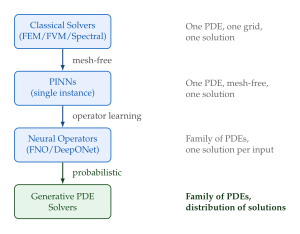
The marriage of deep learning and differential equations is not entirely new. Physics-Informed Neural Networks (PINNs), introduced by Raissi, Perdikaris, and Karniadakis in 2019, showed that one can embed PDE residuals directly into a neural network's loss function and obtain mesh-free approximate solutions. But PINNs, for all their elegance, are single-instance solvers: you train a network to solve one specific PDE with one specific set of initial and boundary conditions. Change the initial temperature distribution, the shape of the domain, or the viscosity coefficient, and you must start over.
The breakthrough of the last five years has been the shift from solving one PDE instance to learning the operator that maps PDE parameters to solutions. Neural operators-most famously the Fourier Neural Operator (FNO) and DeepONet-learn mappings between infinite-dimensional function spaces, so that a single trained model can produce solutions for an entire family of PDEs, evaluated at any desired resolution.
But even neural operators have a fundamental limitation: they are deterministic. They output a single “best guess” solution, typically the conditional mean under a squared-error loss. For many physical systems, especially turbulent flows, chaotic dynamics, and ill-posed inverse problems, the conditional mean is not a physically meaningful quantity. It is a blurred average of many possible states, much as the average face of all humans looks like no one in particular.
Key Idea.
From Deterministic Surrogates to Generative PDE Solvers The key conceptual leap of this chapter is the realisation that PDE solving can be cast as a generative modelling problem. Instead of predicting a single solution , we learn the distribution over solution fields conditioned on PDE parameters (initial conditions, boundary conditions, coefficients, domain geometry). Sampling from this distribution yields diverse, physically plausible solution fields, each respecting the governing equations. This perspective unifies forward simulation, inverse problems, data assimilation, and uncertainty quantification under a single probabilistic umbrella.
The two generative architectures that have proven most powerful in this context are Transformers and diffusion models:
Transformers bring global self-attention over discretised fields, enabling the resolution of long-range spatial dependencies and the handling of irregular, non-Cartesian geometries that defeat convolutional approaches.
Diffusion/score-based models cast PDE solving as an iterative denoising process governed by stochastic differential equations, naturally producing distributions over solution fields and enabling plug-and-play conditioning on sparse observations and physics constraints.
A roadmap for this chapter
This chapter is designed to be largely self-contained. We assume familiarity with basic PDE concepts (the heat equation, the wave equation, boundary conditions) at the level of a first undergraduate course, and with the deep learning fundamentals covered in Chapter ch:deeplearning of this book. Everything else-PINNs, neural operators, Transformer variants, diffusion formulations on function spaces-is developed from scratch with full mathematical detail, worked examples, and TikZ illustrations.
Here is what lies ahead:
A First Look at PDEs and Why They Matter (Section A First Look at PDEs and Why They Matter): We recall the classification of PDEs into elliptic, parabolic, and hyperbolic types, and motivate each class with a flagship physical application. We introduce the Navier–Stokes equations and the associated Clay Millennium Prize Problem-one of the seven greatest unsolved problems in mathematics.
The Computational Bottleneck (Section The Computational Bottleneck): We quantify why classical solvers are expensive, what the “curse of dimensionality” means for parametric PDEs, and why repeated-query settings (design optimisation, uncertainty quantification, Bayesian inversion, real-time control) demand fundamentally new approaches.
Physics-Informed Neural Networks (Section Physics-Informed Neural Networks): We develop the PINN framework rigorously, derive the physics-informed loss, discuss automatic differentiation for computing PDE residuals, and analyse the failure modes (spectral bias, gradient pathologies, multi-term loss balancing). We cover causality-aware training and gradient-rebalancing remedies.
Neural Operator Learning (Section Neural Operator Learning): We formalise the concept of a solution operator mapping input functions to output functions, develop DeepONet and the Fourier Neural Operator from first principles, and discuss theoretical approximation guarantees.
Transformer-Based PDE Solvers (Section Transformer-Based PDE Solvers): We cover Galerkin Transformers, GNOT, Transolver, HAMLET, PiT, physics-attention, PDE-conditional Transformers (Unisolver), and foundation-model pretraining approaches (MPP, CoDA-NO, ICON, PDEformer).
Diffusion and Score-Based Models for PDEs (Section Diffusion and Score-Based Models for PDE Simulation): We develop the theory of diffusion models on function spaces, derive physics-informed diffusion (PIDMs), discuss DiffusionPDE, conditional diffusion for forecasting and data assimilation, CoCoGen, and flow-matching approaches for fast sampling.
Applications by PDE Family (Sections Poisson and Laplace-Type Elliptic PDEs–Coupled and Multiphysics PDE Systems): We walk through each major PDE class-Poisson/Laplace, Burgers, Navier–Stokes, shallow water, Helmholtz, Maxwell, Stefan, Cahn–Hilliard, Schrödinger, and coupled multiphysics systems-showing how Transformers and diffusion models have been applied, with results, figures, and critical analysis.
Turbulence and Generative Modelling (Section Generative Modelling for Turbulence): A dedicated treatment of the turbulence problem, including GAN-era approaches, diffusion for turbulent flow generation, CoNFiLD, GenCFD, and the interplay between spectral accuracy and generative diversity.
Inverse Problems and Uncertainty Quantification (Section PDE-Constrained Inverse Problems): We formalise PDE-constrained inverse problems, develop plug-and-play diffusion priors, RED-DiffEq for full waveform inversion, and InverseBench as a community benchmark.
Benchmarks and Evaluation (Section Benchmarks and Evaluation Practice): We survey PDEBench, PINNacle, and emerging evaluation standards, discussing metrics beyond (energy norms, spectral fidelity, conservation residuals).
Open Problems and the Road Ahead (Section Open Problems and Future Challenges): We discuss the Clay Millennium Prize Problem on Navier–Stokes existence and smoothness, the role of ML in conjecture generation for PDEs, and frontier challenges including discretisation-agnostic generation, real-time turbulence, and generative PDE foundation models.
Exercises (Section Pen-and-Paper Exercises): A comprehensive collection of exercises ranging from pen-and-paper derivations to coding projects.
Remark 1 (Notation).
Throughout this chapter, we denote the spatial domain by , its boundary by , the solution field by (or for systems), and the PDE parameters (coefficients, source terms, boundary data) collectively by . We write , , and for the gradient, divergence, and Laplacian operators, respectively. Neural network parameters are denoted by or to distinguish them from PDE parameters .
A First Look at PDEs and Why They Matter
Partial differential equations are the mathematical language of continuum physics. Wherever a quantity varies smoothly in space and time-temperature, pressure, electric potential, probability density-its evolution is typically governed by a PDE\@. In this section, we revisit the three fundamental types of second-order linear PDEs (elliptic, parabolic, hyperbolic), introduce their flagship physical incarnations, and build toward the Navier–Stokes equations that will serve as the running example throughout this chapter.
The three archetypes
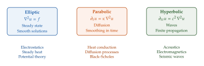
Consider a general second-order linear PDE in two independent variables : (General2nd) The discriminant classifies the equation:
Elliptic (): steady-state problems, e.g., the Laplace equation . Solutions are smooth and encode equilibrium configurations.
Parabolic (): diffusion and heat conduction, e.g., . Information propagates at infinite speed but is smoothed over time.
Hyperbolic (): wave propagation, e.g., . Information propagates at finite speed along characteristics; discontinuities (shocks) can form.
Example 1 (The Poisson equation in electrostatics).
The electric potential generated by a charge distribution in a domain satisfies the Poisson equation: (Poisson) with boundary conditions on (Dirichlet) or on (Neumann). This is an elliptic PDE\@. Its solutions are smooth in (analytic, in fact, if is smooth), and uniqueness follows from the maximum principle.
From a machine learning perspective, the interesting problem is the parametric Poisson equation: given a family of charge distributions , learn the operator mapping source terms to potentials. This is exactly the setting where neural operators shine.
Example 2 (The heat equation).
The temperature in a conducting medium with thermal diffusivity evolves according to: (HEAT) with initial condition and appropriate boundary conditions. This is a parabolic PDE\@. The solution smooths out any initial irregularities as time progresses-a property that will become important when we discuss why deterministic surrogates tend to “blur” their predictions.
Example 3 (The wave equation).
The displacement of a vibrating membrane or acoustic medium satisfies: (WAVE) with wave speed . This is a hyperbolic PDE\@. Unlike the heat equation, discontinuities in the initial data propagate without smoothing-they travel as waves at speed .
The Navier–Stokes equations: beauty and terror
The incompressible Navier–Stokes equations govern the motion of a viscous, incompressible fluid: (Momentum) where is the velocity field, is the pressure, is the (constant) density, is the kinematic viscosity, and represents external body forces. Equation is the momentum equation (Newton's second law for a fluid element), and Equation is the incompressibility constraint (conservation of mass for a constant-density fluid).
The nonlinear advection term is what makes the Navier–Stokes equations simultaneously beautiful and terrifying. It couples the velocity field to itself, creating feedback loops that can amplify small perturbations into the chaotic, multi-scale structures we call turbulence.
Definition 1 (Reynolds number).
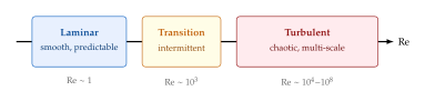
The Reynolds number is the dimensionless ratio of inertial to viscous forces: (Reynolds) where is a characteristic velocity scale, is a characteristic length scale, and is the kinematic viscosity. At low (creeping flow), viscosity dominates and flow is laminar. At high (e.g., for pipe flow), inertia dominates and flow transitions to turbulence.
Kolmogorov's theory of turbulence
In 1941, Andrey Kolmogorov proposed a statistical theory of fully-developed turbulence that remains one of the most profound insights in fluid dynamics. His key hypotheses:
Energy cascade: Energy is injected into the flow at large scales (the integral scale ), cascades through a hierarchy of progressively smaller eddies, and is finally dissipated by viscosity at the Kolmogorov microscale .
Universal scaling: In the inertial range (scales between and ), the energy spectrum follows the celebrated power law: (Kolmogorov) where is the wavenumber and is the mean energy dissipation rate per unit mass.
The Kolmogorov microscale is given by: (Kolmogorov ETA) and the ratio of the largest to smallest scales goes as . In three dimensions, the number of grid points needed for DNS scales as: (DNS COST) For an aircraft wing at , this gives grid points-far beyond current computational capabilities.
Insight.
Why Generative Models Matter for Turbulence The Kolmogorov energy cascade reveals a fundamental mismatch between deterministic neural surrogates and turbulent flows. A network trained with loss learns the conditional mean, which averages out the fine-scale fluctuations that carry much of the physically relevant information (drag, mixing rates, noise generation). Generative models, by learning the full conditional distribution , can sample individual realisations that preserve the correct energy spectrum, including the law in the inertial range.
The Clay Millennium Prize Problem
In the year 2000, the Clay Mathematics Institute announced seven Millennium Prize Problems, each carrying a reward of $1,000,000. The Navier–Stokes problem is among them:
Conjecture 1 (Navier–Stokes existence and smoothness).
What makes this problem so difficult? The nonlinear advection term can amplify vorticity through the vortex stretching mechanism. In two dimensions, vortex stretching is absent, and global regularity was proven by Ladyzhenskaya in the 1960s. In three dimensions, vortex stretching can potentially concentrate vorticity to a point, creating a singularity. Despite decades of effort by the world's best analysts, neither existence nor blow-up has been proven in general.
Remark 2 (What ML can and cannot do).
Machine learning cannot solve the Millennium Prize Problem in its mathematical sense-the question demands a rigorous proof, not a numerical experiment. However, ML-based simulations can:
Generate high-resolution flows that probe near-singular behaviour, providing evidence for or against blow-up scenarios.
Discover new scaling laws and invariants in turbulent flows that might inspire analytical approaches.
Assist in formal theorem proving for PDE regularity results (connecting to the topics in the chapter on Generative Models for Mathematics).
We revisit this in Section Open Problems and Future Challenges.
The Computational Bottleneck
We have seen that DNS of turbulent flows is prohibitively expensive. But the computational bottleneck extends far beyond turbulence. In this section, we examine three settings where classical PDE solvers become a fundamental limitation, motivating the need for neural surrogates and generative alternatives.
The many-query problem
In many scientific and engineering workflows, one needs to solve not one PDE but a family of PDEs, parametrised by varying inputs:
Design optimisation: Finding the wing shape that minimises drag involves evaluating the Navier–Stokes equations for thousands of candidate geometries. Each evaluation requires a full PDE solve.
Uncertainty quantification (UQ): If the material properties (e.g., permeability in a porous medium) are uncertain, one must propagate this uncertainty through the PDE solver. Monte Carlo sampling requires – PDE solves.
Bayesian inversion: Estimating subsurface geological properties from seismic measurements requires evaluating the forward PDE model at every step of an MCMC chain.
Real-time control: Active flow control (e.g., reducing drag on a vehicle) requires evaluating the PDE model in milliseconds, far faster than any classical solver can operate.
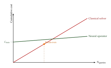
In all these settings, the PDE solver is called inside a loop, and the total computational cost is: (Total COST) where is the cost of a single solve and can range from hundreds to millions.
Key Idea.
Amortised Computation via Neural Operators The fundamental promise of neural operators is amortised computation: invest a large upfront cost to train the model on representative PDE instances, then enjoy near-instant evaluation for any new input. If training costs and inference costs , the break-even point is: (Breakeven) For turbulent CFD, can be hours while is milliseconds, making the break-even point remarkably low.
The curse of dimensionality
Classical PDE solvers discretise the domain into a mesh with degrees of freedom. For a -dimensional domain with grid points per dimension, . The cost of a single solve typically scales as:
for explicit time-stepping (e.g., forward Euler),
for spectral methods with FFT,
for sparse direct solvers (– depending on dimension and method).
When the PDE is parametric-i.e., we want solutions for all in some parameter space -the effective dimensionality of the problem is . For high-dimensional parameter spaces (e.g., uncertain spatially-varying coefficients discretised on a grid), can be in the thousands, and traditional methods like sparse grids or polynomial chaos expansions break down.
What classical solvers do well-and where they fall short
Before we dive into neural alternatives, it is important to acknowledge what classical numerical methods excel at:
Rigorous error bounds: Finite element methods come with a priori and a posteriori error estimates in well-defined norms (, , etc.).
Conservation properties: Finite volume methods conserve mass, momentum, and energy by construction.
Mesh adaptivity: Adaptive mesh refinement (AMR) can concentrate resolution where it is needed (e.g., near shocks or boundary layers).
Decades of engineering validation: These methods have been tested and trusted in safety-critical applications (aircraft certification, nuclear reactor design, weather prediction).
Neural surrogates do not (yet) provide rigorous error bounds, do not conserve physical quantities by construction, and have limited track records in safety-critical settings. The goal is not to replace classical solvers but to complement them-using neural models for fast exploration and reserving classical solvers for final validation.
Caution.
Never deploy a neural PDE surrogate in a safety-critical application without careful validation against classical solvers or experimental data. Neural surrogates can fail silently and catastrophically on out-of-distribution inputs.
The landscape of neural approaches to PDEs
The neural PDE solving landscape can be organised along two axes:
Single-instance vs. operator learning: Does the model solve one specific PDE (PINNs) or learn the solution operator for a family (neural operators)?
Deterministic vs. generative: Does the model output a single solution (point estimate) or a distribution over solutions?
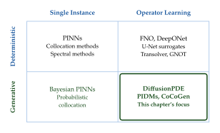
Table 1 provides a quantitative comparison of the key approaches along several dimensions.
| Method | Scope | Output | Mesh-free? | UQ? | Inverse? |
| PINNs | Single | Deterministic | Yes | Limited | Limited |
| FNO | Operator | Deterministic | No | No | No |
| DeepONet | Operator | Deterministic | Yes | No | No |
| Transolver | Operator | Deterministic | Yes | No | No |
| DiffusionPDE | Operator | Generative | No | Yes | Yes |
| PIDMs | Operator | Generative | No | Yes | Yes |
| FunDPS | Operator | Generative | Yes | Yes | Yes |
| FNO has “zero-shot super-resolution” on uniform grids but does not handle unstructured meshes. | |||||
Exercise 1.
Consider a Darcy flow problem (elliptic PDE) on a grid. A finite element solver takes 2 seconds per solve on a single CPU core. A trained FNO takes 5 milliseconds per inference on a GPU\@. Training the FNO requires 10,000 PDE solutions (generated offline) and 4 hours of GPU time.
What is the break-even number of queries , assuming the offline data generation is the dominant training cost?
An engineer needs to run a Bayesian inversion with 50,000 MCMC steps. How much wall-clock time does this take with (a) the FE solver and (b) the FNO?
Discuss the trade-offs: what might go wrong with the FNO approach?
Physics-Informed Neural Networks
We now arrive at one of the most influential ideas in scientific machine learning: using a neural network as a trial function for a PDE, and training it by penalising the PDE residual evaluated at random collocation points. This simple but powerful idea-the Physics-Informed Neural Network (PINN)-was popularised by Raissi, Perdikaris, and Karniadakis (2019) and has since spawned an enormous literature.
The core idea
Suppose we wish to solve a PDE of the general form: (General) subject to initial condition and boundary condition for . Here is a (possibly nonlinear) differential operator and encodes boundary conditions (Dirichlet, Neumann, Robin, periodic, etc.).
The PINN approach is breathtakingly simple:
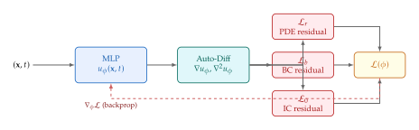
Represent by a neural network: Let be a multilayer perceptron (MLP) with parameters , taking as input and returning the predicted solution value.
Compute PDE residuals via automatic differentiation: The partial derivatives , , etc. are computed exactly (up to floating-point precision) using the chain rule through the network's computational graph. No finite differences or mesh are needed.
Minimise a physics-informed loss: The loss function penalises the PDE residual, boundary residual, and initial condition residual at randomly sampled collocation points: (LOSS) where: (LOSS Residual)
Example 4 (PINN for the 1D Burgers equation).
Consider the viscous Burgers equation on : (Burgers) with , initial condition , and boundary conditions .
The PINN loss is:
For small , the solution develops a sharp shock around , and this is precisely where standard PINNs struggle (see Section Failure modes of PINNs).
Automatic differentiation for PDE residuals
The magic of PINNs lies in automatic differentiation (AD). Unlike finite differences, which introduce truncation errors and require a mesh, AD computes exact derivatives through the computational graph.
For a network with layers: (MLP) where is the activation function. The key observation is that each partial derivative can be computed by the chain rule: (Chainrule) where denotes the hidden representation at layer . Higher-order derivatives (needed for PDEs like the heat equation or Navier–Stokes) require multiple applications of this chain rule.
Remark 3 (Computational cost of higher-order AD).
Computing -th order derivatives via AD requires passes through the computational graph. For the Cahn–Hilliard equation (which involves ), this means four nested differentiation passes, each multiplying the computational cost and potentially accumulating floating-point errors. This is one reason why higher-order PDEs are particularly challenging for PINNs.
Failure modes of PINNs
Despite their elegance, PINNs suffer from several well-documented failure modes that limit their applicability to challenging PDEs. Understanding these failures is essential both for improving PINNs and for appreciating why generative alternatives are needed.
Spectral bias
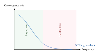
Neural networks with smooth activations (tanh, sigmoid, softplus) have an intrinsic preference for low-frequency functions. This spectral bias causes PINNs to learn the low-frequency components of the solution first and converge extremely slowly (or not at all) on high-frequency features such as:
Sharp shocks in Burgers' equation,
Rapidly oscillating solutions of the Helmholtz equation,
Fine-scale turbulent structures.
Mathematically, the Neural Tangent Kernel (NTK) of an MLP with smooth activations has eigenvalues that decay rapidly with frequency. For a target function with significant high-frequency content, the corresponding NTK eigenvalues are small, and the gradient flow converges slowly along those directions.
Theorem 1 (Spectral bias in the NTK regime, informal).
For an MLP with smooth activations in the infinite-width (NTK) regime, the rate of convergence of the -th Fourier mode of the residual is proportional to the -th eigenvalue of the NTK\@. For smooth activations, rapidly as , implying exponentially slow learning of high-frequency features.
Multi-term loss balancing
The PINN loss is a weighted sum of multiple terms. The weights , , are hyperparameters that dramatically affect convergence. If is too small, the network may satisfy the PDE in the interior but violate boundary conditions; if is too small, the network may interpolate the initial/boundary data but ignore the physics.
Definition 2 (Gradient-statistics-based rebalancing).
Wang et al. (2021) proposed dynamically adjusting the weights based on gradient statistics: (Rebalance) where the numerator is the maximum gradient magnitude of the residual loss and the denominator is the mean gradient magnitude of the -th loss term. The weights are updated with exponential moving average: with controlling the smoothing rate.
Gradient pathologies
A deeper issue is that the gradients and can point in conflicting directions. Stiff PDEs (where the PDE residual varies by many orders of magnitude across the domain) exacerbate this: the optimiser may oscillate between reducing the interior residual and the boundary residual, making net progress extremely slow.
Wang, Teng, and Perdikaris (2021) provided a systematic analysis of these gradient pathologies, showing that the condition number of the effective Hessian of the PINN loss can be astronomically large for stiff systems, leading to training failure.
Causality violation
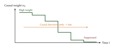
For time-dependent PDEs, collocation points are typically sampled uniformly over the entire spatiotemporal domain . This means the optimiser simultaneously tries to fit the solution at (where the initial condition is known) and at (where the solution must be propagated through the dynamics). The network may “cheat” by fitting later times without correctly propagating from the initial condition, resulting in solutions that are smooth and low-residual but physically meaningless.
Definition 3 (Causal training).
Wang, Sankaran, and Perdikaris (2022) introduced causal training, which reweights the temporal collocation points to enforce a causal ordering: (Causal) where the causal weights are defined as: (Causal Weights) with controlling the causal strictness. When the residual at earlier times is large, for later times is exponentially suppressed, forcing the optimiser to first fit the solution at early times before moving to later times.
Remedies and extensions
The failures of vanilla PINNs have spurred an impressive body of work on improved training strategies. We highlight several:
Fourier feature embeddings: Replacing the raw input with random Fourier features (where is a random matrix) alleviates spectral bias by mapping the input to a higher-dimensional space where all frequencies are equally accessible. This is closely related to the random Fourier features kernel approximation.
Adaptive activation functions: Jagtap and Karniadakis (2020) introduced learnable parameters in the activation function (e.g., where is a scaling factor and is learnable), allowing the network to adapt its frequency response during training.
Domain decomposition (XPINNs): The domain is divided into subdomains, each with its own PINN, with interface conditions enforced via additional loss terms. This reduces the effective complexity each network must capture.
Time-stepping PINNs: Instead of solving over the entire time interval at once, the interval is divided into windows , and a PINN is trained sequentially on each window, using the previous solution as the initial condition.
Curriculum learning: Start training on an easier version of the PDE (e.g., higher viscosity) and gradually increase the difficulty, allowing the network to build up its representation incrementally.
Key Idea.
PINNs as a Stepping Stone PINNs demonstrated a fundamental principle: physics can be encoded as a soft constraint in a neural network's loss function. This idea transcends PINNs and permeates the entire field of physics-informed machine learning, including the generative models we will study later. Physics-informed diffusion models, for instance, add PDE residuals as “virtual observables” during diffusion training-a direct descendant of the PINN philosophy.
From single instances to operators: the limits of PINNs
The fundamental limitation of PINNs is that they are single-instance solvers. A PINN trained to solve the Burgers equation with and initial condition cannot, without retraining, solve the same equation with or .
Proposition 1 (PINN retraining cost).
For a parametric PDE family with parameter configurations, the total PINN training cost is: where is the cost of training a single PINN\@. This linear scaling in is unacceptable for design optimisation or UQ, where can be –.
This limitation motivates the operator learning paradigm, which we develop in the next section: instead of learning the solution for fixed parameters , we learn the operator that maps parameters to solutions across the entire family.
Exercise 2.
Implement a PINN for the 1D Burgers equation (Example 4) using PyTorch or JAX\@.
Train with interior collocation points, boundary points, and initial condition points.
Plot the learned solution as a heatmap and compare with the analytical solution (obtainable via the Cole–Hopf transformation).
Experiment with the loss weights , , . What happens when is set to zero?
Implement causal training (Definition 3) and compare the convergence with and without causality enforcement for (a regime where shocks are sharp).
Exercise 3 (Spectral bias experiment).
Consider the 1D Poisson equation on with and
Train a PINN with a architecture and tanh activation. Plot the residual spectrum (Fourier transform of ) at epochs 100, 1000, and 10000. Which frequencies converge first?
Repeat with Fourier feature embeddings where with . How does the convergence change?
Neural Operator Learning
In the previous section we saw how PINNs embed physics into a neural network's loss function to solve one PDE instance at a time. Each new set of initial conditions, boundary conditions, or coefficients requires retraining from scratch. This is rather like hiring a brilliant chef who can cook exactly one dish: delicious, but impractical for running a restaurant.
The conceptual leap of neural operator learning is to move from learning a single function to learning the operator that maps an input function (coefficient field, initial condition, forcing term) to the corresponding solution function. Once is learned, we can evaluate it on any new input function at inference time with a single forward pass-no retraining, no iterative solver, no mesh.
Key Idea.
Operator Learning: Amortised PDE Solving Traditional solvers and PINNs spend all their computational effort on a single PDE instance. Operator learning amortises this cost over a family of PDE instances: a large offline training cost is paid once, after which each new instance is solved in milliseconds. This is the same amortisation principle that underlies variational autoencoders (Chapter ch:vaes), normalising flows (Chapter 18), and amortised variational inference more broadly.
This section develops the mathematical foundations of operator learning, presents the two most important architectures-DeepONet and the Fourier Neural Operator-derives key theoretical guarantees, and concludes by identifying the fundamental limitations that motivate the generative approaches of the remaining sections.
The Operator Learning Problem
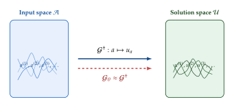
Function spaces and the solution operator
We begin by formalising the setting. Let be a bounded domain, and consider a parametric family of PDEs: (Parametric) where is an input function that parametrises the PDE. The input could be:
A spatially varying coefficient field (e.g., the permeability in Darcy flow),
An initial condition (e.g., for the heat equation),
A forcing term (e.g., the right-hand side in Poisson's equation),
A combination of the above.
For each admissible input , the PDE has a unique solution .1 The solution operator is the mapping that sends to :
Definition 4 (Solution Operator).
The superscript denotes the true (data-generating) operator; the goal of operator learning is to find an approximation , parametrised by learnable parameters .
Remark 4 (Infinite-dimensional input and output).
Unlike standard supervised learning, where both input and output are finite-dimensional vectors, operator learning maps between infinite-dimensional spaces. This is the fundamental challenge: the input is a function with uncountably many degrees of freedom, and so is the output . Any practical implementation must discretise both and onto a finite grid or point cloud, but the architecture should-ideally-be independent of the discretisation resolution.
The data-driven formulation
In practice, we are given a training dataset of input–solution pairs: (Dataset) where each pair is generated by running a classical PDE solver (finite elements, finite volumes, spectral methods) on the input . The functions are drawn from some distribution on (e.g., a Gaussian random field), and both and are observed on discrete grids.
The operator learning problem is then: (Objective) where the norm is approximated by a discrete quadrature rule on the observation grid.
Universal approximation for operators
The theoretical foundation for operator learning was laid remarkably early-long before the deep learning revolution-by Chen and Chen in 1995.
Theorem 2 (Universal approximation for operators - Chen & Chen, 1995).
Let be a compact subset of a Banach space , and let be a continuous (nonlinear) operator, where is compact. Then for every , there exist positive integers and , constants (for and ), and points such that (CHEN CHEN) where is any continuous non-polynomial activation function.
This theorem says two profound things:
Any continuous operator can be approximated to arbitrary accuracy by a finite-rank architecture involving two sub-networks, one acting on the input function (evaluated at fixed sensor locations ) and one acting on the output query point .
The input function need only be observed at finitely many sensor locations-we do not need the entire function, only its values at representative points.
Historical Note.
From Kolmogorov to Chen–Chen The Chen–Chen theorem can be seen as an operator-valued extension of Cybenko's theorem (1989) for universal approximation of functions by neural networks, which is itself inspired by Kolmogorov's superposition theorem (1957). The progression is elegant: Kolmogorov showed that any continuous function of variables can be represented as a superposition of continuous functions of one variable; Cybenko showed that shallow neural networks are universal function approximators; and Chen–Chen showed that a particular two-sub-network architecture universally approximates continuous operators between function spaces. This chain of ideas-from Hilbert's 13th problem (1900) to modern neural operators-spans over a century of mathematics.
DeepONet
The Chen–Chen theorem provides an existence result, but it took until 2019–2021 for Lu, Jin, Pang, Zhang, and Karniadakis to transform it into a practical deep learning architecture: DeepONet (Deep Operator Network).
Architecture
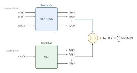
DeepONet is a direct realisation of equation . It consists of two sub-networks:
Branch network : Takes as input the values of the input function at fixed sensor locations and outputs a vector of coefficients .
Trunk network : Takes as input a query location and outputs a vector of basis function values .
The output is their inner product:
Definition 5 (DeepONet).
The DeepONet approximation of the solution operator is: (Deeponet) where are the combined parameters of the branch and trunk networks.
The beauty of this factorisation is its interpretability: the trunk network learns a set of basis functions for the output space, while the branch network learns the coefficients of the expansion as a function of the input . This is precisely a learned generalisation of classical basis expansions such as Fourier series, proper orthogonal decomposition (POD), and reduced basis methods.
Insight.
DeepONet as a Learned Basis Expansion In classical reduced-order modelling, one computes a fixed orthonormal basis (e.g., via SVD/POD of the solution snapshots) and approximates , where the coefficients are found by projection. DeepONet replaces the fixed basis with a learnable one (the trunk network) and replaces linear projection with a nonlinear encoder (the branch network). This added flexibility allows DeepONet to capture phenomena that require many POD modes with far fewer “neural basis functions.”
Training procedure
Training DeepONet requires a dataset of input–solution pairs , where each is observed at (possibly different) query locations . The loss is the mean squared error over all observations: (LOSS)
Key practical considerations include:
Sensor placement. The sensor locations are fixed across all training samples and must be chosen before training. A uniform grid is a common default, but adaptive or random sensor placement can improve performance for problems with localised features.
Query point sampling. The query points can be sampled randomly from at each training iteration, acting as a form of data augmentation and stochastic quadrature.
Data generation. Each training pair requires a full PDE solve. For expensive PDEs, this can be the bottleneck. Common strategies include using coarser meshes for training data, multi-fidelity approaches, or augmenting with physics-informed losses.
Number of basis functions . Increasing gives more capacity but also more parameters. In practice, works well for many benchmark problems.
Physics-informed DeepONet
Just as PINNs augment data losses with PDE residuals, we can create a physics-informed DeepONet (PI-DeepONet) by adding a residual penalty. Since the trunk network maps a query point to the output value, we can differentiate the DeepONet output with respect to using automatic differentiation and penalise the PDE residual: (PI Deeponet)
This hybrid approach reduces the amount of labelled data needed by injecting known physics, and is particularly valuable when full-field solution data is expensive to generate.
Caution.
Differentiating Through the Branch Network In PI-DeepONet, automatic differentiation is applied to the trunk network's contribution (since we differentiate with respect to the spatial coordinate ), not the branch network's contribution. However, because the output is a product , differentiating with respect to acts only on the trunk: . The branch coefficients are treated as constants with respect to the spatial derivatives, which simplifies the implementation considerably.
Worked example: DeepONet for Darcy flow
Example 5 (DeepONet for steady-state Darcy flow).
Consider the two-dimensional Darcy flow equation on the unit square : (Darcy) with Dirichlet boundary conditions on . Here is the permeability field and is a fixed forcing (say, ). We want to learn the operator .
Data generation. We draw permeability fields from a Gaussian random field: , where if and otherwise (creating a two-phase piecewise-constant field), with and . Each permeability is discretised on a grid, giving sensor values. Solutions are computed using a second-order finite element solver on the same grid.
Architecture. The branch network is a CNN with four convolutional layers (since the input is a image), producing a vector . The trunk network is an MLP with four hidden layers of width 128, taking and outputting .
Training. We minimise the loss using Adam with learning rate , decayed by a factor of 0.5 every 100 epochs, for 500 epochs total. At each iteration, 256 random query points are sampled per input function.
Results. On a held-out test set of 200 permeability fields, the trained DeepONet achieves a relative error of approximately 1.8%, with each evaluation taking 2,ms on a single GPU-a speedup of roughly compared to the finite element solver.
Variants and extensions
Several important extensions of the basic DeepONet architecture have been proposed:
POD-DeepONet. Replace the learnable trunk with the leading POD modes of the training solutions: are fixed, and only the branch network is trained. This reduces the parameter count and can improve accuracy when the solution manifold is well-approximated by a linear subspace.
MIONet (Multiple-Input Operator Network). Extends DeepONet to handle multiple input functions (e.g., both an initial condition and a forcing term) via separate branch networks whose outputs are combined by a tensor product: (Mionet)
Stacked DeepONet. For time-dependent problems, the output at time is predicted using the solution at as input: . This autoregressive approach enables long time horizon predictions, though error accumulation remains a challenge.
Fourier Neural Operator
While DeepONet builds on the Chen–Chen universal approximation theorem, the Fourier Neural Operator (FNO), introduced by Li, Kovachki, Azizzadenesheli, Liu, Bhatt, Stern, and Anandkumar (2021), takes an entirely different-and arguably more elegant-route. The key insight is both simple and powerful: if the PDE solution operator involves convolutions and global interactions, why not parameterise the integral kernel directly in Fourier space?
The key insight: convolutions in Fourier space
Many PDEs-particularly linear ones-have solution operators that can be expressed as integral transforms: (Integral) where is the Green's function or integral kernel. For translation-invariant kernels (), this becomes a convolution, and the convolution theorem tells us: (CONV Theorem) where denotes the Fourier transform and the Fourier coefficients. Convolution in physical space becomes pointwise multiplication in Fourier space.
This is the founding observation of FNO: instead of learning the kernel in physical space (which requires parameters for an -point discretisation), we directly learn the Fourier-space weights , which requires only parameters if we truncate to Fourier modes.
Key Idea.
Parameterising Kernels in Fourier Space The FNO replaces the expensive integral kernel in physical space with a learnable Fourier-space filter: a complex-valued matrix that multiplies the Fourier coefficients of the hidden representation. Since physical solutions of PDEs are typically smooth, the Fourier spectrum decays rapidly, and truncating to the lowest modes introduces negligible error while reducing the parameter count from to , where is the hidden channel dimension.
The Fourier layer
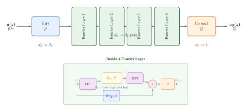
The FNO consists of a sequence of Fourier layers, each performing a spectral convolution combined with a pointwise nonlinearity. A single Fourier layer maps a function to as follows:
Definition 6 (Fourier Layer).
Let be the input to the -th layer. The Fourier layer is defined by: (Layer) where:
and define a pointwise linear transformation (local “bypass”),
is a pointwise nonlinear activation (typically GeLU),
is the spectral convolution operator: (Spectral CONV)
Here is a learnable complex-valued tensor that acts by matrix–vector multiplication on each retained Fourier mode separately.
Let us unpack the spectral convolution step by step:
Forward FFT: Compute for all retained modes .
Fourier-space multiplication: For each retained mode , apply the learnable weight: , where .
Mode truncation: Set all Fourier modes with to zero. This is both a regulariser and the source of the model's efficiency.
Inverse FFT: Compute , returning to physical space.
The pointwise linear term plays a crucial role: it captures local, high-frequency interactions that are lost due to Fourier mode truncation. Together, the spectral convolution handles global structure while the pointwise term handles local features.
Full FNO architecture
The complete FNO pipeline consists of three stages:
Lift: A pointwise linear layer lifts the input from the physical dimension to a higher-dimensional hidden representation of dimension : (LIFT)
Fourier layers: A stack of Fourier layers (typically ): (Stack)
Project: A pointwise MLP projects from the hidden dimension back to the output dimension (typically 1): (Project)
Zero-shot super-resolution
One of the most remarkable properties of FNO is its discretisation invariance: because the learnable parameters live in Fourier space and are indexed by frequency rather than grid point, the same trained model can be evaluated on grids of any resolution.
Proposition 2 (Zero-shot super-resolution).
Let denote the FNO evaluated on an -point discretisation. If the FNO is trained on resolution , it can be evaluated at resolution without retraining by:
Computing the FFT on the finer -point grid,
Applying the same Fourier-space weights to the retained modes (zero-padding any modes between and ),
Computing the inverse FFT on the -point grid.
The additional high-frequency modes () pass through unchanged (or are set to zero), preserving the spectral content learned during training.
This zero-shot super-resolution is impossible for grid-based methods like standard CNNs, which have a fixed input/output resolution determined by their architecture.
Remark 5 (Resolution transfer in practice).
While zero-shot super-resolution is theoretically exact for band-limited functions, in practice there is some accuracy degradation when transferring to much higher resolutions, because: (i) the training data distribution at resolution may not fully represent the fine-scale features visible at resolution , and (ii) aliasing effects during training can introduce biases. Nevertheless, FNO typically maintains reasonable accuracy at to resolution transfer, which is a significant advantage over grid-based methods.
Complexity analysis
Let us compare the computational cost of different approaches for an operator on a -dimensional domain discretised with points per dimension (total grid size ):
1.3
Method Complexity per layer Notes Dense integral kernel Full kernel Standard convolution (CNN) Local kernel size Graph Neural Operator neighbours FNO (Fourier layer) FFT-based
Proposition 3 (FNO complexity).
A single Fourier layer of the FNO with grid size , hidden dimension , and retained modes per dimension has:
Computational cost: , dominated by the FFT ( per channel) for large , and by the Fourier-space multiplication () for small .
Parameter count: -independent of the grid resolution .
This should be contrasted with a dense integral operator, which requires parameters and operations. For a 2D problem with and , the FNO parameters scale as rather than -a reduction of five orders of magnitude.
FNO for benchmark PDEs
The FNO has been benchmarked on several canonical PDE problems. We highlight two here.
Example 6 (FNO for 2D Darcy flow).
Consider again the steady-state Darcy flow equation on . The input is a piecewise-constant permeability field on a grid (sub-sampled to for training), and the output is the pressure field .
Setup. training pairs, test pairs. FNO with Fourier layers, , modes in each spatial dimension. Trained with Adam () for 500 epochs.
Results. Relative test error: (versus for a standard CNN and for DeepONet on the same data). Inference time: 0.005,s per sample on GPU. Resolution transfer: the model trained on achieves error when evaluated on without retraining.
Example 7 (FNO for 2D Navier–Stokes).
Consider the 2D incompressible Navier–Stokes equations in vorticity form on the periodic torus : (NS) where is the vorticity, is recovered from via the Biot–Savart law, and is a fixed forcing.
Task. Given the vorticity field at the first time steps, predict the vorticity at the next steps (i.e., the operator maps to ).
Results at (mildly turbulent):
1.2
Method Relative error (%) U-Net 19.8 Truncated FNO-2D 15.6 FNO-3D (space + time) 1.56
The FNO-3D variant treats the temporal dimension as a third spatial dimension and applies the Fourier layer in all three dimensions simultaneously, achieving dramatically better results.
FNO variants
The success of FNO has inspired a rich family of extensions:
U-FNO. Adds U-Net-style skip connections between Fourier layers at different resolutions, improving multi-scale modelling.
Geo-FNO. Extends FNO to non-rectangular domains by learning a diffeomorphism that maps the irregular domain to a regular one where FFT can be applied.
Factorised FNO (F-FNO). Factorises the -dimensional Fourier convolution into one-dimensional convolutions along each axis, reducing complexity from to .
Adaptive FNO. Learns which Fourier modes to retain rather than using a fixed truncation, adapting the spectral representation to the problem structure.
Spherical FNO (SFNO). Replaces the Cartesian FFT with spherical harmonic transforms, enabling FNO on the sphere-crucial for weather and climate modelling. This variant has been central to recent breakthroughs in data-driven weather prediction.
Theoretical Foundations
Having seen the practical architectures, we now develop the theoretical machinery that underpins neural operator learning. The central questions are: Can neural operators approximate any continuous operator? How efficiently? And what are the fundamental limits?
Universal approximation revisited
We have already stated the Chen–Chen theorem (Theorem 2) for DeepONet-type architectures. The analogous result for FNO was established by Kovachki, Lanthaler, and Mishra (2021):
Theorem 3 (Universal approximation for FNO, informal).
Let be a continuous operator on the -dimensional torus (i.e., with periodic boundary conditions). For every , there exist choices of (number of Fourier layers), (hidden dimension), and (number of retained modes) such that the FNO satisfies: (Universal) for any compact set .
Remark 6 (Periodicity assumption).
The FNO universal approximation result requires periodic boundary conditions (the torus ), because the discrete Fourier transform implicitly assumes periodicity. For non-periodic domains, Geo-FNO or domain-extension techniques are needed to maintain theoretical guarantees. This is an important caveat: naively applying FNO to a problem with Dirichlet boundary conditions can produce Gibbs-like oscillations near .
Approximation rates
Universal approximation tells us that neural operators can approximate any continuous operator, but it says nothing about how many parameters are needed. Approximation rate theory addresses this crucial question.
Theorem 4 (Approximation rate for Lipschitz operators, simplified).
Suppose is Lipschitz continuous with constant , and the input distribution is supported on a compact set whose Kolmogorov -width satisfies for some . Then there exists a DeepONet (or FNO) with parameters in the branch (or Fourier modes) such that: (RATE) where depends on , the ambient dimension, and the constant .
The rate mirrors the decay of the Kolmogorov -width, confirming the intuition that operator learning is easy when the solution manifold is effectively low-dimensional.
The Kolmogorov -width
The Kolmogorov -width is a fundamental concept from approximation theory that quantifies the “intrinsic dimensionality” of a set of functions.
Definition 7 (Kolmogorov -width).
Let be a compact subset of a Banach space . The Kolmogorov -width of in is: (Nwidth) where the outer infimum is over all -dimensional linear subspaces .
In plain English: is the best worst-case error when approximating elements of by elements of an optimal -dimensional linear subspace. If decays rapidly (e.g., exponentially), then can be well-represented by a small number of basis functions, and operator learning is “easy.” If decays slowly (e.g., algebraically), the solution manifold is inherently high-dimensional, and any method-classical or neural-faces fundamental difficulties.
Example 8 (Kolmogorov -width for different PDE families).
Elliptic PDEs (e.g., Darcy flow with smooth permeability): The solution manifold has exponentially decaying -width: . This explains why both reduced basis methods and neural operators achieve excellent accuracy with modest numbers of basis functions/modes.
Parabolic PDEs with smooth initial data (e.g., heat equation): Similar exponential decay, because the diffusion operator rapidly damps high-frequency components.
Hyperbolic PDEs with shocks (e.g., Burgers' equation, Euler equations): The -width decays only algebraically: . The presence of shock discontinuities at varying locations makes it impossible to approximate the solution set well with any linear subspace. This is the Kolmogorov barrier, and it applies equally to POD, reduced basis methods, and-in a certain sense-to the linear component of neural operators.
Insight.
The Kolmogorov Barrier and Nonlinear Approximation The Kolmogorov -width measures the best linear approximation. Neural operators, being nonlinear, can potentially bypass this barrier. For instance, a nonlinear encoder can learn to “register” or “align” shocks before projecting onto a low-dimensional subspace, achieving approximation rates that beat the linear -width. This is one of the key theoretical motivations for using deep neural networks rather than linear methods for problems with moving discontinuities. However, the extent to which practical neural operators actually achieve this nonlinear bypass is still an active area of research.
Connection to reduced basis methods
Neural operators can be understood as nonlinear generalisations of classical reduced-order models (ROMs). The connection is illuminating:
1.3
Reduced Basis / POD Neural Operator Basis functions Fixed from SVD Learned (trunk net / Fourier modes) Coefficients Linear projection Nonlinear encoder (branch net / Fourier layers) Approximation Linear: Nonlinear: -width barrier Cannot beat Can potentially beat Offline cost Moderate (SVD + Galerkin) High (training neural network) Online cost Very low (matrix solve) Very low (forward pass)
Remark 7 (When do neural operators outperform ROMs?).
Neural operators tend to outperform classical ROMs when:
The solution manifold has slowly decaying Kolmogorov -width (e.g., transport-dominated problems with moving shocks),
The mapping from parameters to coefficients is highly nonlinear,
The problem involves high-dimensional parameter spaces where interpolation-based ROMs suffer from the curse of dimensionality.
For problems with rapidly decaying -width and smooth parameter-to-coefficient maps (e.g., coercive elliptic PDEs with smooth coefficients), classical ROMs can be competitive with or even superior to neural operators, particularly when interpretability and certified error bounds are desired.
Error decomposition
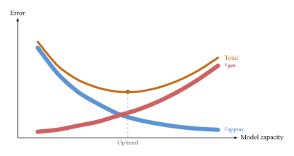
The total error of a neural operator can be decomposed into three sources:
Theorem 5 (Error decomposition for neural operators).
The total error of a trained neural operator satisfies: (Error Decomp) where:
is the approximation error: the best error achievable within the neural operator's hypothesis class, regardless of data or training. This depends on the architecture (number of layers, modes, hidden dimension).
is the generalisation error: the gap between the training loss and the population loss, arising from finite training data. By standard learning theory, this scales as .
is the optimisation error: the gap between the training loss achieved and the global minimum, arising from the non-convexity of the training landscape.
This decomposition guides architecture design: increasing model capacity (more layers, modes, channels) reduces but may increase , while more data reduces , and better optimisers (learning rate schedules, pre-training, curriculum learning) reduce .
Limitations of Deterministic Neural Operators
Neural operators represent a transformative advance over classical solvers and PINNs for many applications. Yet they have fundamental limitations that no amount of architectural engineering can overcome. Understanding these limitations is essential for appreciating why generative approaches to PDE solving-the subject of the remaining sections of this chapter-are not merely interesting alternatives but, for many problems, a necessity.
Regression to the mean
The most severe limitation of deterministic neural operators is the regression-to-the-mean problem. When trained with a mean squared error (MSE) loss , the optimal predictor is the conditional mean: (COND MEAN)
For deterministic PDEs with unique solutions, this is perfectly fine-the conditional mean is the unique solution. But for chaotic or turbulent systems, the mapping from input to solution is effectively one-to-many: small perturbations in the input (below the measurement precision) lead to vastly different solutions. In such cases, the conditional mean is a blurry average of many possible states, and is not itself a physically realisable solution.
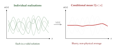
To make this more precise, consider the vorticity field of a turbulent flow. The energy spectrum (Kolmogorov's law) characterises the cascade of energy from large to small scales. The conditional mean suppresses high-frequency fluctuations, leading to a steeper energy spectrum that violates the scaling. This is not an artefact of poor training; it is a mathematical consequence of the MSE objective.
Proposition 4 (MSE suppresses variance).
Let be a random field with conditional mean and conditional variance . Then for any deterministic predictor , the MSE-optimal predictor is , and: (MSE Decomp) The first term is the irreducible error (aleatoric uncertainty) and cannot be reduced by any deterministic predictor. The only way to capture the variability in is to produce a distribution over solutions.
No uncertainty quantification
A deterministic neural operator outputs a single point prediction with no accompanying measure of confidence. In safety-critical applications-structural engineering, nuclear reactor design, weather forecasting-practitioners need to know how uncertain the prediction is, not just the prediction itself.
There are post-hoc approaches to add uncertainty estimates to deterministic models:
Ensemble methods: Train independent neural operators and use the spread of their predictions as a proxy for uncertainty. However, ensemble diversity may not correlate with true posterior variance, especially in out-of-distribution regions.
MC Dropout: Apply dropout at inference time and interpret the variation across forward passes as uncertainty. This is computationally cheap but often underestimates uncertainty.
Bayesian neural operators: Place priors on the network weights and perform (approximate) posterior inference. This is principled but computationally demanding for large-scale models.
None of these approaches produce calibrated, high-dimensional distributions over solution fields. Generating diverse, physically consistent samples from the solution distribution requires a fundamentally different approach: generative modelling.
Fixed discretisation for grid-based methods
While FNO enjoys discretisation invariance (via the Fourier representation), many other neural operators-particularly those based on CNNs, U-Nets, or graph neural networks-are tied to a specific mesh or grid resolution. Changing the resolution requires retraining or introduces interpolation errors. Even for FNO, the zero-shot super-resolution property degrades for large resolution jumps, as discussed in Remark 15.
Training data requirements
Each training pair requires a full PDE solve, which can be expensive. For 3D time-dependent problems (e.g., turbulent Navier–Stokes), a single high-fidelity simulation may require hours on a GPU cluster. Generating thousands of such pairs for training can cost more than the savings gained at inference time, especially if the model is used for only a few evaluations.
The break-even point depends on the application:
Many-query settings (design optimisation, Bayesian inversion, real-time control): The offline training cost is amortised over thousands or millions of queries, making neural operators highly cost-effective.
Few-query settings: The upfront data generation and training cost may not be justified. This motivates physics-informed approaches that reduce or eliminate the need for labelled data.
Motivating generative approaches
The limitations above can be summarised in a single observation: deterministic neural operators learn the wrong quantity for stochastic, chaotic, or ill-posed problems. They learn the conditional mean , when what we need is the conditional distribution .
Key Idea.
From Deterministic Operators to Generative PDE Solvers The move from deterministic to generative PDE solving is motivated by three needs:
Physical fidelity: Samples from are individually physical and respect the correct statistical structure (energy spectra, intermittency, spatial correlations), unlike the blurry conditional mean.
Uncertainty quantification: The distribution provides calibrated uncertainty estimates over the entire solution field, not just point-wise confidence intervals.
Downstream tasks: For risk assessment, rare-event estimation, and robust design, we need the tails of the distribution, which are invisible to conditional-mean predictors.
The generative modelling toolkit developed in the earlier chapters of this book-variational autoencoders, normalising flows, GANs, score-based diffusion models-provides exactly the machinery needed to learn and sample from . The remaining sections of this chapter show how to adapt each of these frameworks to the infinite-dimensional, physics-constrained setting of PDE solving.
Exercises
Exercise 4 (DeepONet for the heat equation).
Consider the one-dimensional heat equation on with and initial condition .
Write down the solution operator in terms of the eigenfunctions . How many eigenmodes contribute significantly for large ? Relate this to the Kolmogorov -width of the solution set.
Design a DeepONet architecture for this problem. How many sensor points and basis functions would you use? Justify your choices.
How would a physics-informed DeepONet loss differ from the purely data-driven loss for this problem? Write down the explicit residual term.
Argue that for large , the operator is “easy” in the sense that a very small suffices. What happens as ?
Exercise 5 (FNO mode selection).
Consider a family of solutions on of the form where the Fourier coefficients satisfy for some .
If the FNO retains modes, show that the truncation error satisfies:
For the Navier–Stokes equations at Reynolds number , the Kolmogorov dissipation scale is , suggesting significant Fourier content up to wavenumber . How many FNO modes would you need to capture all physically relevant scales at ?
Compare the FNO parameter count (with the from part (b)) to the parameter count of a dense kernel approach. At what Reynolds number does FNO become infeasible?
Exercise 6 (The conditional mean is not enough).
Let be the solution to the inviscid Burgers equation on with periodic boundary conditions and random initial condition , where is fixed and is a random phase.
Show that for any such that no shock has yet formed, the conditional mean is identically zero. (Hint: use the symmetry of the phase distribution.)
Explain why this conditional mean is not a valid solution of the Burgers equation (except for the trivial ).
How would a generative model address this problem? What would a sample from the conditional distribution look like?
Compute the MSE of the optimal deterministic predictor and compare it to the MSE of a generative model that produces a single sample. Which has lower expected MSE? Which produces more physically meaningful outputs?
Challenge 1 (From DeepONet to FNO: bridging the architectures).
Show that a single-layer FNO with Fourier modes and no pointwise bypass () can be written in the DeepONet form for an appropriate choice of , , and . What are the “trunk” basis functions? What role does the FFT play in computing the “branch” coefficients?
Hint: Expand the spectral convolution using the discrete Fourier basis and identify the branch outputs with the Fourier coefficients of the input, multiplied by the learnable weights.
Transformer-Based PDE Solvers
In the preceding sections we developed two families of neural PDE solvers: Physics-Informed Neural Networks (PINNs), which embed the PDE residual into the loss function of a single-instance neural network, and Neural Operators (FNO, DeepONet), which learn mappings between infinite-dimensional function spaces from data. Both families have achieved remarkable successes, yet both suffer from a common architectural limitation: they struggle to capture long-range spatial dependencies in the solution field.
PINNs use multilayer perceptrons (MLPs) whose receptive field is, in principle, global but whose spectral bias causes them to learn low-frequency components first and high-frequency details painfully slowly. The Fourier Neural Operator circumvents this by operating directly in spectral space, but at the cost of being restricted to uniform grids-a serious limitation for the complex, irregular geometries that arise in real-world engineering (airfoils, turbine blades, blood vessels, city-scale wind simulations).
Enter the Transformer. Originally developed for natural language processing, the Transformer's core mechanism-self-attention- computes pairwise interactions between all tokens in a sequence, regardless of their distance. When the “tokens” are discretisation points (or patches, or learned physical states) of a PDE domain, self-attention naturally captures the long-range, nonlocal interactions that PDEs encode: a pressure wave at one end of a pipe affects the velocity field everywhere; a vortex shed from the leading edge of an airfoil influences the wake far downstream.
Key Idea.
Transformers as Universal Nonlocal Operators The self-attention mechanism computes a weighted integral over the entire spatial domain at each point, making it a natural discrete approximation to the integral operators that appear throughout PDE theory (Green's functions, Fredholm operators, potential theory). This connection is not merely an analogy: as we shall prove in this section, attention can be viewed as a discretised Galerkin projection onto a data-dependent subspace.
This section provides a comprehensive and mathematically rigorous treatment of Transformer-based PDE solvers. We begin with the conceptual and mathematical motivations (Section Why Transformers for PDEs?), then proceed through the major architectures in roughly chronological order: the Galerkin Transformer (Section The Galerkin Transformer), GNOT (Section GNOT: General Neural Operator Transformer), Transolver (Section Transolver), HAMLET (Section HAMLET: Graph Transformer Neural Operator), and PiT (Section PiT: Position-induced Transformer). We then cover the emerging wave of PDE foundation models and conditioning strategies (Section PDE-Conditional Transformers and Foundation Models), in-context operator learning (Section In-Context Operator Learning), and finally the PINNsFormer architecture that replaces the MLP backbone of PINNs with a Transformer (Section PINNsFormer).
Why Transformers for PDEs?
To appreciate why Transformers have become the dominant architecture for PDE solving, we must understand three foundational insights: (i) self-attention captures long-range dependencies that local convolutions miss, (ii) attention operates on sets rather than grids, enabling natural handling of irregular meshes, and (iii) attention is intimately related to the integral operators that constitute the backbone of PDE theory.
Self-attention captures long-range dependencies
Consider an elliptic PDE such as the Poisson equation on a domain with Dirichlet boundary conditions. The solution at any interior point depends on the source term and the boundary data everywhere in the domain, through the Green's function: (Green) where is the Green's function of the Laplacian on and is the boundary data.
This integral representation reveals a fundamental nonlocality: the solution at depends on the values of at every point . A convolutional neural network with a kernel of size has a receptive field that grows only linearly with depth (or as after layers), and therefore requires very deep architectures to capture global interactions. The standard self-attention mechanism, by contrast, computes pairwise interactions between all input tokens in a single layer:
Definition 8 (Scaled dot-product attention).
Given query, key, and value matrices and , the scaled dot-product attention is (Attention) Each row of the output is a weighted average of all rows of , where the weights depend on the pairwise similarities between queries and keys.
In the PDE context, we interpret the rows as spatial discretisation points (mesh nodes, collocation points, or patches). The output at each point is a function of all other points, mediated by learned similarity weights. This is precisely the discrete analogue of the integral operator in equation .
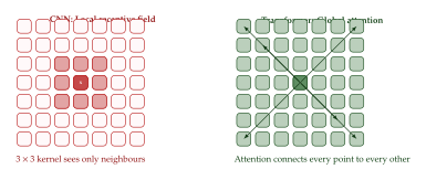
Irregular mesh handling
A second, equally important advantage is that attention operates on sets of tokens, not on regular grids. A convolutional layer assumes that its input lives on a regular Cartesian lattice; applying a CNN to an unstructured triangular mesh or a point cloud requires either interpolation to a regular grid (losing geometric fidelity) or specialised graph-convolutional layers (which reintroduce locality).
Self-attention has no such constraint. Given points with arbitrary coordinates , we simply encode each point into a query-key-value triplet and let attention determine the interaction weights. Positional information can be injected through positional encodings-either fixed (sinusoidal, random Fourier features) or learned-so that the model is aware of the spatial locations without requiring a grid structure.
Remark 8 (Positional encodings for PDE domains).
Unlike in NLP, where positional encodings encode a one-dimensional sequence order, PDE discretisations live in for (and sometimes higher for parametric problems). Common choices include:
Sinusoidal encodings applied independently to each coordinate: , , with frequencies chosen as in the original Transformer.
Random Fourier features: with drawn from a Gaussian, approximating a stationary kernel.
Learned MLPs that map to an embedding vector, allowing the model to discover task-specific spatial representations.
Attention as an integral operator
The deepest reason that Transformers are well suited to PDE solving is that self-attention is a discretised integral operator. Consider a general kernel integral operator of the form (Integral OP) where is a kernel function and is the input function. This is a Fredholm integral operator of the second kind-precisely the form that appears in Green's function representations, boundary element methods, and the integral formulations of many PDEs.
Now discretise the domain with points carrying quadrature weights . The discrete approximation is (Discrete Integral) Comparing with the attention output at position : (ATTN Integral) we see that the softmax-normalised attention weights play the role of the kernel evaluated at the discretisation points, and the value vectors play the role of the function values.
Proposition 5 (Attention as a discretised kernel integral).
Let be a parametric kernel, where is the feature representation of point and are learned projection matrices. Then the softmax attention output computes, for each discretisation point , a Monte Carlo approximation to the normalised kernel integral: (Normalised Integral) where the integration measure is replaced by the empirical measure .
Proof.
Write , , . Then the attention output at position is which is a normalised empirical average-precisely the Monte Carlo approximation to with the uniform empirical measure .
Insight.
The connection between attention and integral operators is not just a mathematical curiosity. It suggests a principled design strategy: we can import decades of knowledge about numerical integration-quadrature rules, adaptive refinement, preconditioning- into the design of attention mechanisms for PDEs. This insight underpins several of the architectures we study in this section.
The quadratic bottleneck and its remedies
The elephant in the room is computational cost. Standard self-attention has time and memory complexity, where is the number of tokens (discretisation points). For a 2D PDE on a grid, , and the attention matrix has entries-far too large for most GPUs.
This has motivated a rich line of work on efficient attention for PDE solving:
Linear attention: Replace softmax with a kernel factorisation so that , reducing complexity to . This is the approach of the Galerkin Transformer.
Cross-attention with learned queries: Introduce learnable “slice” queries and compute cross-attention . This is the approach of Transolver.
Sparse or local attention: Restrict attention to local neighbourhoods plus a few global tokens, as in Longformer-style architectures.
Downsampling + global attention: Pool the discretisation to a coarser representation, apply global attention, and upsample. This multiscale strategy is used by GNOT and several others.
Caution.
Not all efficient attention variants are created equal for PDEs. Sparse local attention can miss precisely the long-range interactions that motivated the use of Transformers in the first place. Architectures that reduce the token count via physics-aware compression (e.g., Transolver's intrinsic physical states) tend to perform better than generic sparsification methods that are agnostic to the PDE structure.
The Galerkin Transformer
The Galerkin Transformer, introduced by Cao (NeurIPS 2021), was one of the first architectures to draw a rigorous connection between Transformer attention and classical numerical methods for PDEs. The key insight is that standard softmax attention approximates a Petrov–Galerkin projection, and that by choosing a different normalisation, one can obtain an attention mechanism that corresponds to a Galerkin projection-a cornerstone of finite element theory.
Background: the Galerkin method
Recall the classical Galerkin method for solving a linear PDE. Given an operator equation in a Hilbert space , we seek an approximate solution in a finite-dimensional subspace such that the residual is orthogonal to : (Galerkin Classical) This yields the linear system where and .
Definition 9 (Galerkin projection).
The Galerkin projection of a function onto with respect to a bilinear form is the element satisfying (Galerkin PROJ) When , this reduces to orthogonal projection.
From softmax attention to Galerkin attention
Cao observed that standard softmax attention computes: (Softmax ATTN) where the normalisation is row-wise: each query produces its own probability distribution over keys. This corresponds to a Petrov–Galerkin method where the test functions (queries) and trial functions (keys) live in different spaces.
The Galerkin Transformer replaces this with two alternative attention mechanisms:
Galerkin-type attention.
Instead of row-wise softmax normalisation, Galerkin-type attention normalises column-wise over the keys, corresponding to a symmetric Galerkin projection where test and trial functions come from the same space: (Galerkin ATTN) Here is computed first (at cost ), and then multiplied by (at cost ), giving an overall linear complexity of instead of .
Fourier-type attention.
An alternative normalisation normalises column-wise over the queries: (Fourier ATTN) The name “Fourier” comes from the observation that when the keys and values are Fourier basis functions, this computation reduces to computing Fourier coefficients-a discrete Fourier-like transform.
Theorem 6 (Galerkin attention as orthogonal projection).
Let denote the subspace spanned by the value vectors, and let denote the orthogonal projection onto in the -inner product. Then the Galerkin attention output , when , computes (Galerkin PROJ THM) where is the empirical cross-covariance between keys and values. When the key vectors form an orthonormal basis (), this is exactly the orthogonal projection of onto the column space of through the basis .
Proof.
Write the attention output at row : Define . When , we have forming a discrete orthonormal system. The matrix acts as a change-of-basis matrix from the -representation to the -representation. Multiplying first computes the expansion coefficients of in the -basis (inner products ) and then maps them to the -basis, which is exactly the orthogonal projection onto the -span through the -basis.
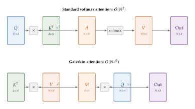
Architecture details
The full Galerkin Transformer architecture wraps the Galerkin attention mechanism in a standard Transformer encoder-decoder structure:
Input encoding: The input function (e.g., initial condition, forcing term, or coefficient field) is evaluated at discretisation points. Each point is encoded as to produce a -dimensional token.
Galerkin attention layers: A stack of layers, each consisting of Galerkin multi-head attention followed by a feed-forward network with residual connections and layer normalisation. In the multi-head variant, each head computes: (Galerkin Multihead) and the outputs are concatenated and projected: .
Output decoding: A pointwise MLP maps the final hidden representation to the predicted solution value at each discretisation point. Crucially, the output points need not coincide with the input points-the decoder can interpolate to any desired query location by using cross-attention between query positions and the encoded representation.
Example 9 (Galerkin Transformer for Darcy flow).
Consider the steady-state Darcy flow equation on the unit square : (Darcy) with Dirichlet boundary conditions . The operator learning task is: given the permeability field (sampled from a Gaussian random field), predict the solution .
On the Darcy flow benchmark (from the FNO paper), the Galerkin Transformer achieves a relative error of approximately on resolution test data, competitive with FNO () while using roughly the same number of parameters (M). Crucially, the Galerkin Transformer can be evaluated on resolutions different from the training resolution without retraining, since its attention mechanism is resolution-invariant.
Historical Note.
The connection between attention and Galerkin methods was anticipated by the numerical PDE community's long history of using integral operators and spectral methods. The Galerkin method itself dates back to Boris Galerkin's 1915 paper on elastic rods. The neural attention mechanism, introduced by Bahdanau, Cho, and Bengio in 2014 for machine translation, took nearly seven years to be formally connected to Galerkin projections by Cao (2021). This delay illustrates a recurring theme: deep learning and numerical analysis develop largely independently, and the most fruitful innovations come when researchers bridge the gap between the two communities.
GNOT: General Neural Operator Transformer
While the Galerkin Transformer elegantly reduces attention complexity and connects to classical numerical methods, it was primarily demonstrated on problems with a single input function on a regular grid. Many real-world PDE problems involve multiple heterogeneous inputs-an initial condition, a forcing term, boundary data, and possibly geometric parameters-evaluated on irregular, non-uniform meshes. The General Neural Operator Transformer (GNOT), introduced by Hao, Wang, and co-authors at ICML 2023, addresses these challenges through a carefully designed multi-input, multi-scale architecture.
Problem setup and challenges
GNOT considers the general operator learning problem: given a collection of input functions and scalar parameters (e.g., Reynolds number, viscosity), learn the solution operator (GNOT Operator) where the input functions may be evaluated on different, irregular meshes. For instance, in a fluid–structure interaction problem, the fluid velocity might be known on a tetrahedral mesh while the structural displacement is given on a surface triangulation.
The key challenges are:
Heterogeneous inputs: Different input types (functions on meshes, scalar parameters, boundary conditions on surface meshes) must be unified into a single representation.
Irregular geometry: The discretisation points are not on a regular grid, precluding the use of FFT-based methods like FNO.
Scale: Real-world meshes can have – nodes, requiring efficient attention.
Heterogeneous attention
GNOT introduces a heterogeneous normalised attention mechanism that handles multiple input types within a unified framework.
Definition 10 (GNOT heterogeneous attention).
Given input types, each producing key-value pairs for , and query tokens from the current representation, GNOT computes: (GNOT Hetero ATTN) where are learned mixing weights satisfying (enforced via softmax over a learnable parameter vector).
This heterogeneous attention allows the model to attend to different input modalities with different attention patterns while producing a unified output representation.
Multi-scale architecture
To handle large meshes efficiently, GNOT uses a multi-scale approach inspired by the Perceiver architecture:
Encoding: Input tokens (from all input types) are projected to a common embedding dimension . Scalar parameters are broadcast to all tokens via an additive bias.
Cross-attention downsampling: A set of learnable latent tokens attends to the full input via cross-attention: (GNOT Cross) where is the concatenation of all input tokens. This reduces the sequence length from to .
Self-attention on latent tokens: Multiple layers of self-attention are applied to the latent tokens, at cost -much cheaper than when .
Cross-attention upsampling: The output tokens at the desired query locations attend back to the processed latent tokens: (GNOT Decode)
The total complexity is , which is linear in when or .
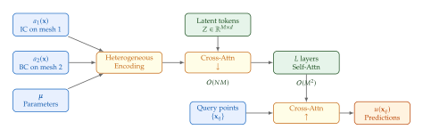
Handling multiple PDE settings
A distinctive feature of GNOT is its ability to handle multiple PDE settings within a single model. By conditioning on scalar parameters (e.g., Reynolds number, Mach number), the same GNOT model can produce solutions for:
Different PDE coefficients (varying viscosity in Navier–Stokes).
Different domain geometries (by encoding geometry as an input function, e.g., a signed distance field).
Different boundary conditions (by including boundary data as a separate input stream).
Proposition 6 (GNOT complexity).
For input types with a total of input tokens, latent tokens, self-attention layers, and embedding dimension , the computational cost of GNOT is (GNOT Complexity) which is linear in the total number of input and output points when with respect to .
Example 10 (GNOT for Navier–Stokes on complex geometries).
Consider the 2D incompressible Navier–Stokes equations on a domain with multiple obstacles (cylinders of varying radii at varying positions). The inputs are:
The signed distance field to the obstacles, evaluated on an irregular triangular mesh with nodes.
The inlet velocity profile, specified on boundary nodes.
The Reynolds number as a scalar parameter.
GNOT with latent tokens and self-attention layers achieves a relative error of on the velocity field, compared to for FNO (which requires interpolation to a regular grid) and for DeepONet.
Transolver
The Transolver (Wu, Hao, Wang, et al., ICML 2024 Spotlight) represents a paradigm shift in how Transformers tokenise PDE domains. Rather than treating each mesh node as a token-which leads to attention for nodes-Transolver introduces the concept of intrinsic physical states: learned, compact representations that capture the underlying physics of different spatial regions. Attention is computed between these physical states rather than between individual mesh nodes, reducing complexity from to where is the number of physical states.
Motivation: physics-aware tokenisation
Consider a complex flow around an airfoil. From a physics perspective, the domain naturally decomposes into a few distinct regions:
The boundary layer (thin region of high shear near the airfoil surface).
The wake region (downstream of the trailing edge).
The freestream region (far from the airfoil, approximately uniform flow).
Stagnation and separation regions (near the leading edge and any flow separation points).
Within each region, the physics is relatively homogeneous: the solution has similar local structure and the governing balances (e.g., inertia vs. viscosity) are similar. This motivates grouping nearby mesh nodes with similar physical behaviour into a single “physical state” token, and computing attention at the level of these physical states.
Key Idea.
From Mesh Nodes to Physical States Traditional Transformer PDE solvers tokenise the mesh: each node becomes a token, and attention operates on tokens. Transolver instead tokenises the physics: it learns to partition the domain into regions of coherent physical behaviour, each represented by a single token. This is analogous to how domain decomposition methods in classical numerical analysis partition a domain into subdomains-but here the partition is learned from data rather than prescribed.
Physics-attention mechanism
The Transolver architecture has two main stages: (i) slice assignment, which maps each of the mesh nodes to one of physical states, and (ii) physics-attention, which computes attention among the physical states and then maps back to the original mesh nodes.
Step 1: Adaptive slice assignment.
Given the input representation (from the previous layer or the input embedding), compute a soft assignment matrix: (Transolver Assign) where is a learnable projection and is a temperature parameter. The column gives the soft membership weights of all nodes to the -th physical state.
Step 2: Aggregate to physical states.
The intrinsic physical state for each slice is computed by a weighted average: (Transolver Aggregate) Stacking these gives , the physics token matrix.
Step 3: Attention among physical states.
Standard multi-head self-attention is applied to the physics tokens: (Transolver ATTN) Since , this costs only .
Step 4: Distribute back to mesh nodes.
The updated physics tokens are distributed back to all mesh nodes using the same assignment matrix: (Transolver Distribute) A residual connection and feed-forward layer complete the block: .
Definition 11 (Physics-attention block).
Theorem 7 (Transolver complexity reduction).
Let a standard Transformer PDE solver with layers have complexity . The Transolver with physical states has complexity (Transolver Complexity) since implies . The speedup factor is , which for a typical setting of mesh nodes and physical states gives a reduction in attention cost.
Proof.
The slice assignment costs (matrix multiplication plus softmax over columns). Aggregation costs (weighted sum). Self-attention costs . Distribution costs . Summing over layers gives the stated bound. Since whenever (which holds by assumption), the term is dominated.
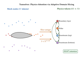
Handling complex geometries
A major strength of Transolver is its ability to handle genuinely complex geometries. The learned slice assignment matrix automatically adapts to the geometry: near a thin boundary layer, many nodes are assigned to the “boundary layer” physical state; in the quiescent freestream, fewer physical states are needed.
Transolver has been demonstrated on:
Airfoils (AirfRANS dataset): Steady-state RANS simulations around parametrically varying NACA airfoil shapes. Transolver achieves state-of-the-art relative error on pressure and velocity fields.
Vehicle aerodynamics (DrivAerNet): 3D external aerodynamics around car bodies, with surface mesh nodes. The scaling makes this tractable where attention would be prohibitive.
Elasticity (von Mises stress on 3D parts): Predicting stress distributions on complex mechanical parts with unstructured tetrahedral meshes.
Example 11 (Transolver for airfoil flow prediction).
Consider predicting the pressure coefficient around NACA 4-digit airfoils at varying angles of attack and Reynolds numbers . The AirfRANS dataset provides RANS simulation data on unstructured meshes with nodes per sample.
With physics tokens and physics-attention layers, Transolver achieves a relative error of on the test set, compared to for PointTransformer, for FNO (on interpolated regular grids), and for GNOT. The learned slice assignments reveal that the model automatically discovers physically meaningful regions: a tight cluster of assignments near the suction peak, a distinct cluster in the wake, and broad clusters in the freestream.
HAMLET: Graph Transformer Neural Operator
While Transolver compresses the mesh into learned physical states, an alternative strategy is to explicitly model the mesh as a graph and use graph Transformers that combine the local inductive bias of graph neural networks (GNNs) with the global attention of Transformers. The HAMLET framework (Bryutkin, Hao, et al., ICML 2024) takes this approach, building a modular architecture that separately encodes PDE-specific information and geometric/mesh information before combining them via a graph Transformer.
Graph structure for PDE domains
Given a mesh with nodes and edges (connecting neighbouring mesh elements), HAMLET constructs a multi-relational graph that encodes:
Spatial adjacency: The original mesh connectivity, providing local structural information.
Multi-scale connections: Edges connecting nodes at different scales of a coarsened mesh hierarchy (obtained via graph coarsening algorithms), enabling efficient multi-resolution information flow.
Boundary-to-interior edges: Explicit connections from boundary nodes to interior nodes, reflecting the influence of boundary conditions on the solution.
Definition 12 (HAMLET multi-relational graph).
The HAMLET graph has relation types, where:
: mesh adjacency edges (from the original mesh).
: multi-scale edges from coarsened mesh levels.
: boundary-to-interior edges.
Each edge carries edge features encoding the relative position and the edge type .
Modular encoder architecture
HAMLET uses a modular encoder that separately processes PDE-specific information and geometric information:
PDE info encoder.
The PDE information at each node (input function values, boundary condition types and values, source terms) is processed by a dedicated MLP: (Hamlet PDE ENC) where is the input function, encodes boundary condition type and value (zero for interior nodes), and is the source term.
Geometry encoder.
The geometric information (node coordinates, edge vectors, element areas) is processed by a separate encoder: (Hamlet GEOM ENC) where encodes local geometric features such as element areas, angles, and curvatures at node .
Fusion.
The two encodings are fused via element-wise multiplication and addition: (Hamlet Fusion)
Graph Transformer layers
The fused representations are processed by a stack of graph Transformer layers. Each layer combines:
Local message passing: A GNN-style update using the mesh adjacency edges, capturing local interactions: (Hamlet Local) where is the neighbourhood of node in the mesh and are graph attention coefficients.
Global attention: A subset of “virtual nodes” (analogous to GNOT's latent tokens) aggregates global information via cross-attention from all mesh nodes, and then broadcasts back. This provides the global receptive field that local message passing lacks.
Multi-relational aggregation: Messages from different edge types are combined with learnable weights: (Hamlet Multirel) where is the message from relation type .
Remark 9 (HAMLET vs. Transolver: complementary strategies).
HAMLET and Transolver represent two complementary approaches to efficient Transformer-based PDE solving. Transolver learns the domain decomposition (via slice assignments) and computes attention among the resulting physical states. HAMLET prescribes the graph structure (from the mesh) and combines local GNN message passing with global virtual-node attention. HAMLET is more natural for problems where the mesh structure carries important information (e.g., adaptive meshes refined in regions of interest), while Transolver excels when the mesh is a discretisation artefact and the underlying physics has coherent large-scale structure.
PiT: Position-induced Transformer
The Position-induced Transformer (PiT), introduced at ICML 2024, takes a different approach to making Transformers efficient for PDEs. Rather than reducing the number of tokens (Transolver) or using a graph structure (HAMLET), PiT exploits the positional structure inherent in PDE discretisations to induce a structured, efficient attention pattern.
Key insight: spatial proximity implies interaction strength
The fundamental observation is that in most PDEs, the interaction strength between two points decays with their spatial distance. For elliptic PDEs, the Green's function typically decays as in dimensions (logarithmically in 2D). For parabolic PDEs, the heat kernel decays exponentially with distance. Even for hyperbolic PDEs where information propagates along characteristics, the relevant interactions are structured by the geometry of the characteristic surfaces.
Proposition 7 (Position-induced attention structure).
Let be a radially decaying kernel, i.e., for a monotonically decreasing function . If the attention weights approximate , then the attention matrix has the structure: (PIT Structure) which is approximately sparse: entries decay rapidly away from the block-diagonal structure induced by spatial proximity.
Position-induced attention
PiT exploits this structure by decomposing the attention computation into two components:
Positional bias.
A positional bias function encodes the spatial relationship between points: (PIT BIAS) where is a small MLP that maps relative positions to a scalar bias. This is added to the attention logits: (PIT ATTN)
Hierarchical attention.
To reduce the cost of computing all pairwise biases, PiT uses a hierarchical decomposition:
Fine level: Full attention within local neighbourhoods of radius (containing points each).
Coarse level: Cluster the domain into supernodes, compute attention among supernodes, and broadcast back.
The total complexity is , which is minimised at giving -sub-quadratic.
Definition 13 (PiT attention).
The PiT attention output at node is (PIT FULL) where is the set of points within distance of , are the local attention weights (with positional bias), is the number of supernodes, are the coarse-level attention weights from node to supernode , and is the aggregated value of supernode .
Connection to numerical PDE methods
PiT's hierarchical attention has deep connections to classical numerical methods:
Multigrid methods: PiT's fine-coarse decomposition mirrors the V-cycle of multigrid: local smoothing on the fine grid followed by correction on a coarser grid. The key difference is that multigrid restricts and prolongs the solution, while PiT restricts and prolongs the attention.
-matrices: The hierarchical matrix (-matrix) framework in numerical linear algebra represents dense matrices arising from integral equations in a compressed, hierarchical format by exploiting the low-rank structure of off-diagonal blocks. PiT's hierarchical attention can be viewed as a learned -matrix.
Fast multipole method (FMM): The FMM computes -body interactions in time by replacing distant interactions with multipole expansions. PiT's supernode aggregation is analogous to the FMM's multipole expansion.
Insight.
PiT demonstrates that the most effective Transformer architectures for PDEs are not generic efficient attention mechanisms (like Performer or Linformer), but rather designs that respect the mathematical structure of PDEs. The spatial decay of Green's functions, the multi-scale nature of PDE solutions, and the hierarchical structure of numerical methods all provide blueprints for attention design. The future of Transformer-based PDE solving lies in ever-tighter integration with classical numerical analysis.
PDE-Conditional Transformers and Foundation Models
The architectures discussed so far-Galerkin Transformer, GNOT, Transolver, HAMLET, PiT-are trained on data from a specific PDE or a specific family of PDEs with varying parameters. A more ambitious goal is to build foundation models for PDEs: large, pretrained Transformers that can solve many different types of PDEs, potentially even generalising to PDE families unseen during training. This subsection covers the key ideas behind PDE-conditional Transformers and the emerging landscape of PDE foundation models.
Unisolver: conditioning on PDE structure
The Unisolver observes that different PDEs have different mathematical structures (different differential operators, different types of nonlinearities), and that a universal solver must be conditioned on these structural properties. The key innovation is a taxonomy of PDE conditioning strategies:
Definition 14 (Domain-wise vs. point-wise PDE conditioning).
Let a PDE be characterised by its differential operator , domain , and boundary/initial conditions.
Domain-wise conditioning: A single embedding vector encodes the global PDE type (e.g., “heat equation”, “Navier–Stokes”, “Helmholtz”) and is added to all tokens: (Domain COND) This is appropriate when the PDE type is uniform across the domain.
Point-wise conditioning: Each discretisation point receives a conditioning vector that encodes the local PDE structure (e.g., the local value of a spatially varying coefficient, the local boundary condition type): (Point COND) This is necessary when the PDE has spatially varying structure (e.g., heterogeneous media, mixed boundary conditions).
Unisolver uses a combination of both conditioning types. The PDE type is encoded as a domain-wise embedding, while spatially varying parameters (coefficients, source terms, boundary conditions) are encoded point-wise. This allows a single model to handle a heterogeneous dataset of PDE problems.
Theorem 8 (Unisolver universality, informal).
Under mild regularity conditions on the PDE families, a sufficiently large Unisolver model (with layers, heads, embedding dimension , and point-wise + domain-wise conditioning) can approximate the solution operator for any PDE in the training distribution to within in the norm, with the number of parameters scaling polynomially in and the dimension of the PDE parameter space.
Zero-shot inference across PDE families
A remarkable finding is that Unisolver, trained on a diverse dataset of PDE families (heat equations, wave equations, advection-diffusion, reaction-diffusion, Burgers, incompressible Navier–Stokes), can perform zero-shot inference on PDE families not seen during training. For example:
Trained on heat and advection-diffusion equations, Unisolver achieves non-trivial accuracy on the convection-diffusion equation (which combines features of both).
Trained on 2D PDEs, Unisolver transfers to 3D versions of the same PDEs by leveraging the coordinate-agnostic nature of the attention mechanism.
This zero-shot capability arises because the point-wise conditioning mechanism allows the model to “read” the local PDE structure from the input, rather than memorising specific PDE types.
Multiple Physics Pretraining (MPP)
The Multiple Physics Pretraining (MPP) framework (McCabe, Blancard, et al., NeurIPS 2024) takes the foundation model idea further by pretraining a large Transformer on a massive, diverse dataset of PDE simulations spanning multiple physics domains.
The key design choices are:
Unified tokenisation.
All PDE solutions are represented as spatial fields on regular or irregular grids. Each spatial patch (e.g., region on a 2D grid) is tokenised as a vector, analogous to Vision Transformer (ViT) patches for images. The number of physical channels varies by PDE type (1 for scalar equations, 3 for velocity fields, etc.), and is handled by a per-channel linear projection to a common embedding dimension.
Physics-aware masking.
During pretraining, random patches of the solution field are masked, and the model is trained to reconstruct them-a masked autoencoder (MAE) objective. The masking ratio is high (75%) to force the model to learn meaningful physical correlations rather than interpolation shortcuts.
Scaling laws.
MPP demonstrates that PDE foundation models obey scaling laws analogous to those observed in large language models. As the model size increases from 10M to 1B parameters and the dataset grows from to PDE simulations, the validation loss decreases as an approximate power law: (MPP Scaling) with and (dataset-dependent). This suggests that continued scaling of PDE foundation models will yield predictable improvements.
Exercise 7 (Scaling law derivation).
Suppose the validation loss of a PDE foundation model follows the scaling law with , , .
- (a)
If the current model has parameters and is trained on simulations, what is the validation loss?
- (b)
To halve the validation loss, by what factor must you increase the model size (keeping the dataset fixed)?
- (c)
Alternatively, by what factor must you increase the dataset size (keeping the model fixed)?
- (d)
Discuss the practical implications: which is more expensive, generating more PDE simulation data or training a larger model?
CoDA-NO: Codomain Attention Neural Operator
The Codomain Attention Neural Operator (CoDA-NO, NeurIPS 2024) introduces a fundamentally different attention mechanism: instead of attending across spatial positions (the domain), CoDA-NO attends across the output channels (the codomain).
Definition 15 (Codomain attention).
Given a representation where is the number of spatial points, is the number of output channels (e.g., for velocity in 3D Navier–Stokes), and is the feature dimension, codomain attention computes: (Codomain ATTN) where are the query, key, and value matrices for spatial point , obtained by linear projections of . The attention is between channels at the same spatial point.
Codomain attention is computationally cheap ( with typically small) and captures the inter-channel correlations that are crucial for multi-field PDEs. For example, in Navier–Stokes, the pressure and velocity fields are coupled through the incompressibility constraint ; codomain attention allows the model to learn these couplings.
CoDA-NO uses codomain attention in combination with spatial attention (either via FNO-style spectral convolutions or Galerkin attention) to capture both spatial and inter-channel dependencies. It is pretrained on a diverse multi-physics dataset and fine-tuned for specific PDE tasks, achieving strong transfer learning performance.
Example 12 (CoDA-NO transfer learning).
CoDA-NO is pretrained on a dataset containing simulations of 2D incompressible Navier–Stokes (vorticity formulation), 2D shallow water equations, and 2D reaction-diffusion systems. When fine-tuned on the compressible Euler equations (not seen during pretraining), CoDA-NO with just 100 fine-tuning samples achieves the same accuracy as an FNO trained from scratch on 1,000 samples-a data efficiency improvement due to transfer. The codomain attention mechanism is particularly effective because it transfers the learned inter-channel correlations (e.g., velocity-pressure coupling) across PDE families with similar multi-field structure.
Towards PDE foundation models: a synthesis
The approaches of Unisolver, MPP, and CoDA-NO represent three complementary pillars of PDE foundation models:
Unisolver: Conditioning the Transformer on PDE structure (domain-wise + point-wise), enabling a single model to handle diverse PDE types.
MPP: Scaling up pretrained Transformers on massive multi-physics datasets, demonstrating predictable scaling laws.
CoDA-NO: Introducing codomain attention for inter-channel transfer learning across PDE families.
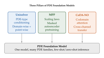
In-Context Operator Learning
One of the most surprising capabilities of large language models is in-context learning: the ability to perform new tasks at inference time simply by providing a few input-output examples in the prompt, without any gradient updates. Can we achieve the same for PDE solving? The answer is yes, and the resulting framework- In-Context Operator Learning (ICON)-represents a fascinating convergence of language modelling ideas and operator learning.
ICON: learning operators from demonstrations at inference
ICON, introduced by Yang, Liu, and co-authors (PNAS, 2023), trains a Transformer to take as input a sequence of input-output function pairs -the “demonstrations”-together with a new query input , and outputs the predicted solution . Crucially, the demonstrations define the operator implicitly: the model must infer what operator maps to from the examples alone.
Definition 16 (In-context operator learning).
Let be an unknown operator (e.g., the solution operator of a PDE). Given demonstration pairs and a query input , the ICON model predicts: (ICON) The model is trained on a meta-distribution over operators: the training loss averages over randomly sampled operators , random demonstrations, and random query inputs.
The architecture processes the demonstration sequence by interleaving each input function and output function as tokens, similar to how a language model processes alternating prompt and response tokens. Self-attention over this interleaved sequence allows the model to:
Identify the pattern relating inputs to outputs (i.e., infer the operator).
Apply the inferred operator to the query input .
Theorem 9 (ICON approximation guarantee, informal).
Under a Bayesian meta-learning framework where the operator is drawn from a prior distribution , the optimal ICON predictor converges to the posterior mean: (ICON Posterior) As , the posterior concentrates on the true operator, and the prediction error vanishes.
Exercise 8 (ICON convergence rate).
Suppose the operator is a linear integral operator with kernel , and the ICON model has access to demonstrations.
- (a)
Show that the posterior mean estimate of has mean squared error when the demonstrations are i.i.d. samples from a Gaussian process prior over input functions.
- (b)
For a nonlinear operator , argue heuristically that the convergence rate depends on the “complexity” of (e.g., the number of terms in a polynomial chaos expansion), and that more demonstrations are needed for more complex operators.
- (c)
Design a toy experiment: choose to be the solution operator of the 1D heat equation with varying initial conditions, and plot the ICON prediction error as a function of for .
PDEformer: PDE as computational graph
While ICON treats the operator as an implicit “black box” to be inferred from demonstrations, the PDEformer (ICLR 2024) takes a more structured approach: it explicitly represents the PDE itself as a computational graph and processes it with a graph Transformer.
The key insight is that any PDE can be represented as a directed acyclic graph (DAG) where:
Leaf nodes: Input variables (, ), parameters (, ), and the unknown function .
Internal nodes: Mathematical operations (differentiation , multiplication, addition, nonlinear functions like , ).
Root node: The PDE residual .
Example 13 (PDEformer graph for Burgers equation).
The viscous Burgers equation is represented as the following computational graph:
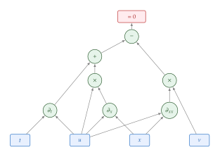
LLM-inspired ideas for PDEs
The success of in-context learning for PDEs has inspired a broader programme of importing ideas from large language models:
Autoregressive PDE solving: Treating the time axis as a sequence and generating solutions autoregressively, one time step at a time, using causal attention. This mirrors how LLMs generate text token by token.
Prompt engineering for PDEs: Providing the model with carefully chosen demonstrations that “steer” the inference towards the desired PDE family or solution regime.
Chain-of-thought for PDEs: Instead of directly predicting the final solution, having the model output intermediate quantities (e.g., the pressure field before the velocity field in a Navier–Stokes solve) as “reasoning steps.”
Retrieval-augmented PDE solving: Augmenting the model's input with retrieved examples of similar PDEs from a database, analogous to retrieval-augmented generation (RAG) in NLP.
Challenge 2 (ICON for coupled multiphysics).
Design an ICON-style in-context operator learning framework for coupled multiphysics problems (e.g., fluid–structure interaction, where the fluid velocity field and the structural displacement field are coupled through boundary conditions at the fluid–solid interface). Address the following questions:
- (a)
How should the demonstration pairs be structured when the operator has multiple input and output fields?
- (b)
How should the attention mechanism handle cross-field interactions (e.g., the coupling between fluid pressure and structural stress at the interface)?
- (c)
What is the expected scaling of the number of demonstrations needed as a function of the number of coupled fields?
PINNsFormer
All the architectures discussed so far in this section are data-driven: they learn operators from input-output pairs generated by classical solvers. The PINNsFormer (Zhao, Fang, and Karniadakis, 2023) takes a different approach: it replaces the MLP backbone of a Physics-Informed Neural Network (PINN, Section Physics-Informed Neural Networks) with a Transformer, combining the physics-informed loss formulation of PINNs with the representational power of Transformers.
Motivation: limitations of MLP backbones
Recall that a standard PINN parameterises the solution as an MLP and minimises the PDE residual at collocation points. MLPs suffer from two well-known limitations:
Spectral bias: MLPs with smooth activation functions (tanh, sigmoid) learn low-frequency components of the solution first and struggle with high-frequency features (shocks, sharp gradients, oscillations).
No temporal structure: The MLP treats time as just another input coordinate, with no architectural mechanism to capture the causal, sequential nature of time evolution.
PINNsFormer addresses both limitations simultaneously.
Pseudo Sequence Generator
The key challenge in applying a Transformer to PINNs is that collocation points are not naturally sequential. PINNsFormer introduces the Pseudo Sequence Generator (PSG), which converts each collocation point into a short sequence by sampling additional points along the time axis.
Definition 17 (Pseudo Sequence Generator).
Given a collocation point and a sequence length parameter , the PSG generates a pseudo-sequence: (PSG) where are uniformly spaced time points: for .
The physical intuition is clear: the solution at depends on the history of the solution at the same spatial location at earlier times. By providing this temporal context as a sequence, the Transformer can capture causal dependencies through its attention mechanism.
Architecture
The PINNsFormer architecture consists of:
Input embedding: Each element of the pseudo-sequence is embedded by a small MLP: (Pinnsformer Embed) where is a sinusoidal positional encoding.
Transformer encoder: A standard Transformer encoder with layers of multi-head self-attention and feed-forward networks processes the sequence . The self-attention uses causal masking (each token can only attend to earlier tokens in the sequence), enforcing the causal structure of time evolution.
Output: The hidden state at the last position () is mapped to the predicted solution value: (Pinnsformer Output)
Physics-informed loss: The loss function is exactly the same as for standard PINNs (equation ): PDE residuals are computed via automatic differentiation through the Transformer, and the loss penalises the residuals at collocation points plus boundary and initial condition violations.
Wavelet activation functions
To further combat spectral bias, PINNsFormer introduces wavelet activation functions that replace the standard smooth activations (tanh, GELU) in the feed-forward layers: (Wavelet Activation) where is the Mexican hat wavelet (negative normalised second derivative of a Gaussian): (Mexican HAT) and is the Morlet wavelet: (Morlet) The parameters are learnable, allowing the model to adaptively select the frequency content of its activations.
Proposition 8 (Wavelet activations mitigate spectral bias).
Let be the true PDE solution with frequency content up to wave number . A PINNsFormer with wavelet activations having learnable scale parameters can represent functions with arbitrarily high frequency content by choosing . In contrast, an MLP with tanh activation has an effective frequency bandwidth that scales only as with network depth in the Neural Tangent Kernel regime.
Example 14 (PINNsFormer for the Burgers equation with a shock).
Consider the inviscid Burgers equation with initial condition on , which develops a shock (discontinuity) at .
Standard PINNs with tanh activations produce severe oscillations near the shock (Gibbs-like ringing) and achieve a relative error of . PINNsFormer with wavelet activations and a pseudo-sequence length of achieves a relative error of and produces a much sharper shock profile. The improvement comes from two sources:
The wavelet activations provide the high-frequency representational capacity needed to resolve the sharp gradient.
The causal Transformer processes the temporal history, allowing it to “track” the characteristics converging to form the shock.
Exercise 9 (Comparing PINNsFormer components).
Design an ablation study for PINNsFormer on the 1D advection equation with and smooth initial condition on with periodic boundary conditions.
- (a)
Compare four configurations: (i) standard PINN (MLP + tanh), (ii) PINN with wavelet activations, (iii) PINNsFormer with tanh activations (Transformer + PSG + tanh), (iv) full PINNsFormer (Transformer + PSG + wavelet). Which component contributes more: the Transformer architecture or the wavelet activations?
- (b)
Vary the pseudo-sequence length and plot the error vs. . Is there an optimal sequence length? What happens when is too large?
- (c)
Replace causal masking with full (bidirectional) attention. How does this affect the solution quality? Does it improve or harm the result for this particular PDE? Explain why.
Comparative analysis and practical guidance
To help the practitioner navigate the growing zoo of Transformer-based PDE solvers, we provide a comparative summary in Table 2.
| Method | Attention type | Complexity | Irregular mesh | Multi-PDE |
| Galerkin Trans.\ | Linear (Galerkin) | Partial | No | |
| GNOT | Cross-attn + latent | Yes | Partial | |
| Transolver | Physics-attn | Yes | No | |
| HAMLET | Graph + virtual nodes | Yes | No | |
| PiT | Hierarchical | Yes | No | |
| Unisolver | Conditioned attn | or linear | Yes | Yes |
| ICON | In-context | Partial | Yes | |
| PINNsFormer | Causal self-attn | Yes | No |
Remark 10 (Choosing the right architecture).
The choice of Transformer architecture depends on the problem characteristics:
Regular grid, moderate : Galerkin Transformer or FNO. The linear complexity and spectral properties are ideal.
Irregular mesh, single PDE family: Transolver (if the domain has coherent physical regions) or HAMLET (if the mesh structure is informative).
Multiple input types, heterogeneous data: GNOT, which was specifically designed for this setting.
Multiple PDE families, desire for zero-shot: Unisolver or MPP-pretrained models.
Physics-informed (no data), single instance: PINNsFormer, which inherits the mesh-free, data-free advantages of PINNs while mitigating spectral bias.
Few-shot, new operator at inference: ICON, which requires no retraining.
We close this section with a forward-looking exercise.
Exercise 10 (Design your own Transformer PDE solver).
You are given the following problem: predict the steady-state temperature distribution inside a 3D heat exchanger with complex internal fin geometry. The inputs are: (i) the inlet temperature profile on an irregular surface mesh ( boundary nodes), (ii) the fin geometry encoded as a signed distance field on a tetrahedral mesh ( nodes), and (iii) the thermal conductivity W/(mK) as a scalar parameter.
- (a)
Which of the architectures in Table 2 would you choose, and why? Consider the mesh size, irregularity, heterogeneous inputs, and the need for parametric generalisation over .
- (b)
Sketch the architecture, specifying: (i) how each input is tokenised, (ii) the attention mechanism, (iii) the output decoder, and (iv) the total computational complexity.
- (c)
Propose a training dataset: what PDE solver would you use to generate the training data? How many samples? What range of and fin geometries?
- (d)
What evaluation metrics would you use beyond relative error? Consider physical quantities of interest (e.g., total heat transfer rate, maximum temperature) and their prediction accuracy.
Diffusion and Score-Based Models for PDE Simulation
“The idea that one can create structure by progressively removing noise is, in retrospect, deeply physical: it is the reverse of the second law of thermodynamics.” - Yang Song
We have now seen two families of neural PDE solvers. Physics-Informed Neural Networks (Section Physics-Informed Neural Networks) embed PDE constraints into the loss function but produce a single deterministic solution per problem instance. Neural operators (Section Neural Operator Learning) learn the mapping from PDE parameters to solutions across entire families, but they too are deterministic: given input parameters , they output a single prediction .
In this section, we make the leap to generative PDE solvers based on diffusion and score-matching. The core idea is both simple and profound: instead of learning a point estimate , we learn the distribution over solution fields conditioned on PDE parameters. Sampling from this distribution produces diverse, physically plausible solution fields-complete with calibrated uncertainty-that respect the governing equations. This is the single most important conceptual shift in this chapter.
Why diffusion models for PDEs?
The mean-regression problem
Consider a turbulent flow governed by the incompressible Navier–Stokes equations at Reynolds number . Two runs with initial conditions that differ by a single-bit perturbation will diverge exponentially, exploring vastly different regions of the solution manifold. Yet if we train a deterministic neural operator by minimising the mean squared error (MSE) over a training set of pairs, the network learns the conditional expectation: (Condmean) This conditional mean is a weighted average over all possible trajectories. For turbulent flows, it produces an unphysical blurred field: the sharp vortices, thin shear layers, and intermittent structures that characterise real turbulence are washed out.
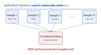
More concretely, suppose the solution distribution is bimodal: , where and are two very different but equally valid turbulent realisations. The conditional mean resembles neither nor . A generative model, by contrast, would sample either or with equal probability, always producing a physically valid field.
Key Idea.
Generative Models Avoid Mean Regression A generative model learns the full conditional distribution , not just its mean. Each sample is a plausible, physically consistent solution field. This is essential for:
Turbulence: capturing sharp structures and intermittency.
Chaotic dynamics: representing sensitivity to initial conditions through ensemble diversity.
Ill-posed inverse problems: quantifying non-identifiability via posterior spread.
Uncertainty quantification: providing calibrated error bars by examining the spread of generated samples.
Why diffusion, specifically?
Among generative models-GANs, VAEs, normalising flows, autoregressive models, diffusion-why have diffusion models emerged as the dominant paradigm for PDE applications? Several reasons:
Iterative refinement parallels multigrid. The reverse diffusion process refines a noisy field over many steps, progressing from coarse, large-scale features to fine details. This coarse-to-fine generation mirrors the multigrid hierarchy used in classical PDE solvers, where one resolves low-frequency error components on coarse grids before refining on fine grids.
Stable training. Unlike GANs, diffusion models are trained with a simple denoising objective that does not require adversarial min-max optimisation. Training is stable, does not suffer from mode collapse, and scales well to high-dimensional fields.
Plug-and-play conditioning. Diffusion models support posterior sampling via guidance: one can inject physics constraints (PDE residuals, conservation laws, boundary conditions) and observational data (sparse sensors, partial measurements) into the sampling process without retraining the model.
Calibrated uncertainty. The stochastic nature of the sampling process naturally yields an ensemble of solutions, whose spread provides a measure of uncertainty.
Forward diffusion = heat equation. The forward noising process is itself a PDE-the heat equation in the space of solution fields! This deep connection between diffusion models and PDEs provides both intuition and mathematical tools.
The physical analogy: forward diffusion as the heat equation
Let us make the connection between diffusion models and PDEs precise. Recall that the forward process of a variance-preserving (VP) diffusion model adds Gaussian noise to a data sample according to the stochastic differential equation (SDE): (Forward SDE) where is the noise schedule and is a Wiener process. The marginal distribution satisfies the Fokker–Planck equation: (Fokkerplanck) When is constant and we drop the drift term, this reduces to the heat equation . The forward diffusion literally heats up the data distribution until it becomes featureless Gaussian noise-thermal equilibrium.
The reverse process, which generates data by starting from noise, can then be understood as anti-diffusion: the creation of structure from chaos, running the heat equation backwards in time. Of course, the heat equation is irreversible in general (information is lost), so the reverse process requires knowledge of the score function , which encodes the structure that must be restored at each time step.
Insight.
Diffusion as Heating and Cooling Forward process: A structured PDE solution field is gradually heated (diffused) until all spatial structure is destroyed and only Gaussian noise remains. This is the thermodynamic arrow of time-entropy increases.\\[4pt] Reverse process: Starting from pure noise, the score function guides the gradual cooling (anti-diffusion) that restores spatial structure. Each denoising step removes some “thermal noise” and refines the field, analogous to annealing in materials science.\\[4pt] The score function is the missing ingredient: It tells us which structure to create at each step, compensating for the information lost during forward diffusion.
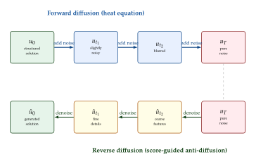
Score-based diffusion on function spaces
PDE solutions live not in but in infinite-dimensional function spaces: the velocity field of a fluid is an element of a Sobolev space , the temperature field lives in , and so on. A truly satisfying theory of diffusion models for PDEs must therefore operate directly on function spaces, independent of any particular discretisation (finite element mesh, spectral coefficients, point cloud).
In this subsection, we develop the mathematical framework for score-based diffusion in infinite dimensions, following the landmark works of Pidstrigach (2022), Kerrigan et al. (2023), and Lim et al. (JMLR, 2025).
The finite-dimensional recap
We begin with a rapid review of the score-based framework in . Let denote the data distribution (e.g., a distribution over discretised solution fields ). The forward noising process is an Itô SDE: (Forward General) where is the drift, is the diffusion coefficient, and is an -dimensional Wiener process. The marginal density evolves according to the Fokker–Planck equation. At the terminal time , we want , a tractable reference distribution (typically ).
Definition 18 (Score function).
The score function of a probability density is the gradient of its log-density: (Score) The score points in the direction of steepest increase of the log-density at each point in space.
The fundamental result of Anderson (1982) states that the forward SDE has a time-reversed counterpart: (Reverse SDE) where is a Wiener process running backwards in time (from to ), and the crucial extra term is precisely the score function scaled by the diffusion coefficient.
Theorem 10 (Anderson's reverse-time SDE, 1982).
In practice, we approximate the score with a neural network trained via denoising score matching: (DSM) where is the tractable transition kernel of the forward SDE (Gaussian for linear drift), and is a positive weighting function.
Remark 11 (Denoising score matching is tractable).
The key insight of denoising score matching (Vincent, 2011; Song et al., 2021) is that one never needs to evaluate the intractable marginal score . Instead, we match the conditional score , which is known in closed form. For the variance-preserving SDE with and : where , giving:
Extension to Hilbert spaces
Now we move to infinite dimensions. Let be a separable Hilbert space (for concreteness, think of where is the physical domain). We wish to define a diffusion process on that perturbs function-valued data .
The first obstacle is the definition of a Wiener process. In finite dimensions, is a standard Brownian motion with identity covariance. In infinite dimensions, the analogous object-a -valued Brownian motion with identity covariance-does not exist as a bona fide -valued process (its sample paths would have infinite norm almost surely). We must use a -Wiener process with a trace-class covariance operator .
Definition 19 (-Wiener process on a Hilbert space).
Let be a symmetric, positive, trace-class operator (i.e., ), with eigenvalues and corresponding orthonormal eigenfunctions . A -Wiener process is the -valued process: (Qwiener) where are independent standard scalar Brownian motions. The trace-class condition ensures that the series converges in .
The covariance operator controls the spatial correlation structure of the noise. A common choice is for some and , yielding a Matérn-like spatial covariance that decays with distance and penalises high-frequency noise.
Caution.
No “white noise” in infinite dimensions In , the standard Wiener process has covariance (white noise). In , the analogous “cylindrical Wiener process” with does not take values in -its sample paths are distributions, not functions. One must always use a trace-class , which smooths out the noise at high frequencies. This has a direct physical interpretation: the noise added during forward diffusion must be spatially correlated, not pixel-independent.
With the -Wiener process in hand, we can define the forward SDE on : (Forward Hilbert) where is a probability measure on (the data distribution over PDE solution fields), is a (possibly nonlinear) drift operator, and is a scalar diffusion coefficient.
Definition 20 (Score function on a Hilbert space).
Let be the law of on . If has a density with respect to a reference Gaussian measure (with covariance ), the score is defined as: (Score Hilbert) where denotes the Fréchet derivative in . In the eigenbasis of : (Score Components)
Theorem 11 (Reverse SDE on Hilbert spaces).
Under regularity conditions on , , and the score , the time-reversed process satisfies: (Reverse Hilbert) with . Note the appearance of rather than just : the covariance operator weights the score correction according to the noise structure.
Remark 12 (The role of in the reverse SDE).
The product in has a clear interpretation: the score correction is applied only along directions in which noise was injected. Eigenvalues of that are zero (or very small) correspond to function-space directions along which no noise was added, and consequently no correction is needed. This ensures that the reverse process respects the regularity class of the forward process.
Score matching in function space
How do we train a score network when lives in a function space? The denoising score matching objective generalises naturally. For the Ornstein–Uhlenbeck forward process , the transition kernel is Gaussian on : (Transition Hilbert) where and .
The conditional score in the eigenbasis of is: (COND Score Hilbert) The function-space denoising score matching loss is: (DSM Hilbert)
Proposition 9 (Discretisation consistency).
Let be a projection onto the first eigenmodes of (or any orthogonal projection), and let be the discretised field. If is parameterised as a resolution-agnostic architecture (e.g., a neural operator that accepts inputs of any resolution), then the function-space loss evaluated on discretisations of increasing resolution converges to the infinite-dimensional loss as . In particular, a model trained on resolution can be applied at resolution without retraining.
This discretisation agnosticism is a major practical advantage: one can train on coarse grids (cheap) and generate on fine grids (expensive but needed only at inference time).
Example 15 (VP diffusion on ).
Consider with the Fourier basis . Let have eigenvalues (the covariance of a mean-zero Gaussian random field with Sobolev regularity ). The -Wiener process is: The noise realisation at any time is a random function that is spatially smooth (it lives in for any ). High-frequency modes () receive negligible noise, so the forward diffusion primarily corrupts the large-scale structure of the solution field.
For the VP forward process with , the noised field at time is: The denoising score matching target for mode is: Note the amplification: the score for high-frequency modes is much larger in magnitude, reflecting the fact that -noise in those modes is very small, so the score must “shout loudly” to correct even small perturbations.
Mathematical rigor: well-posedness
We collect the key conditions under which the infinite-dimensional framework is well-posed.
Assumption 1 (Regularity conditions for function-space diffusion).
We require:
is trace-class on : .
The data measure is absolutely continuous with respect to the Gaussian measure .
The score is -a.e. well-defined and satisfies .
The drift is Lipschitz on uniformly in .
Theorem 12 (Well-posedness of function-space score matching (Lim et al., JMLR 2025)).
Under Assumption 1, the denoising score matching loss is well-defined and finite. Moreover, its unique minimiser (over the class of all measurable functions ) is the true score . The reverse SDE with the true score has a unique strong solution, and the law of coincides with .
Historical Note.
From Pixels to Functions Score-based diffusion models were originally formulated for finite-dimensional data (images, audio). The extension to function spaces was motivated by the need for discretisation-agnostic generative models in scientific computing. Key milestones include:
Pidstrigach (2022): First formulation of score-based generative models on infinite-dimensional spaces, introducing the -Wiener framework.
Kerrigan et al. (2023): Functional diffusion processes with neural operator score networks.
Lim et al. (JMLR, 2025): Rigorous well-posedness theory and convergence guarantees for score matching in function space.
Baldassari et al. (2024): Conditional score-based diffusion for Bayesian inference on function spaces with applications to PDE inverse problems.
DiffusionPDE: joint diffusion over coefficients and solutions
One of the most striking applications of diffusion models to PDEs is DiffusionPDE (Huang et al., NeurIPS 2024), which proposes learning the joint distribution over PDE coefficients (e.g., a spatially varying diffusivity field) and solution fields , simultaneously. This is a conceptually radical idea: rather than viewing the PDE as a fixed constraint that maps , we treat both and as random fields drawn from a joint distribution that encodes the PDE relationship implicitly.
Problem formulation
Consider a parametric PDE of the form: (Parametric PDE) where is a spatially varying coefficient (e.g., permeability in Darcy flow, thermal conductivity in heat transfer) and is the solution. Given a distribution over coefficient fields and the deterministic map defined by the PDE, there is a joint distribution supported on the manifold .
DiffusionPDE learns this joint distribution using a single diffusion model. The data is represented as a multi-channel field: (Multichannel) and the diffusion model is trained on paired samples where is obtained by solving the PDE with coefficient field .
Sparse observation guidance
At inference time, DiffusionPDE can reconstruct full coefficient and solution fields from sparse observations. Suppose we observe the solution at a sparse set of sensor locations with values (where is measurement noise). We wish to sample from the posterior: (Posterior)
This posterior sampling is achieved via classifier guidance applied during the reverse diffusion process. At each denoising step , the unconditional score is augmented with a likelihood gradient: (Guided Score) where is a guidance weight. For Gaussian observation noise with variance : (OBS Likelihood) where is Tweedie's estimate of the clean field from the noisy state at diffusion time : .
PDE constraint guidance
A key innovation of DiffusionPDE is using the PDE residual itself as an additional guidance signal. Since the generated fields should satisfy the PDE, we define a PDE-residual likelihood: (PDE Likelihood) where and are Tweedie estimates of the clean coefficient and solution fields. The total guided score becomes: (Total Guidance)
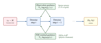
Architecture and training
DiffusionPDE uses a U-Net backbone with the following design choices:
Multi-channel input. The coefficient field and solution field are concatenated as channels of a single spatial field. For systems with multiple solution components (e.g., velocity and pressure in Navier–Stokes), all components are stacked.
Time embedding. The diffusion time is encoded via sinusoidal positional embeddings and injected into each residual block, following the standard DDPM architecture.
Training data. Paired samples are generated by sampling from a prior (e.g., a Gaussian random field) and solving the PDE numerically to obtain .
Loss. The standard -prediction loss: , where and .
Example 16 (DiffusionPDE for Darcy flow).
Consider the 2D Darcy flow equation on : (Darcy) with . The coefficient field represents permeability and is drawn from a log-normal random field: with a Matérn kernel .
DiffusionPDE trains on 10,000 pairs at resolution . At inference, given only random sensor observations of (about 1% of the grid), the guided sampling procedure recovers both and with relative error below 5%. This dramatically outperforms deterministic baselines (FNO, DeepONet) that require substantially more observations.
Proposition 10 (Posterior consistency of guided diffusion).
Let denote the marginal distribution of the diffusion model's generated samples, and let denote the distribution under observation guidance with weight . Under mild regularity conditions, as : where is the MAP estimate. Conversely, as , (the prior). Intermediate values of interpolate between the prior and the MAP estimate, with corresponding (approximately) to the true posterior.
Physics-informed diffusion models
While DiffusionPDE applies physics constraints at inference time (via guidance), an alternative approach embeds physics directly into the training objective. This is the strategy of Physics-Informed Diffusion Models (PIDMs), introduced by Bastek and Kochmann (ICLR 2025).
Motivation: PDE residuals as virtual observables
Recall the PINN philosophy: the PDE residual is treated as a constraint that must hold at every point in the domain. PIDMs import this idea into the diffusion framework. At each training step, the denoised estimate (obtained from the current noise prediction ) should approximately satisfy the PDE. We can therefore add a physics loss to the denoising objective: (PIDM LOSS) where is the Tweedie estimate of the clean sample.
Definition 21 (PIDM training objective).
A Physics-Informed Diffusion Model augments the standard denoising score matching loss with a PDE residual penalty evaluated on the denoised estimate . The full objective is: (PIDM FULL) where is a time-dependent weight that may be annealed during training.
Computing PDE residuals through the denoiser
A subtlety arises: to evaluate , we need spatial derivatives of . Since depends on (a discretised field on a grid), these derivatives must be computed via finite differences on the grid or via spectral methods. The gradient of the physics loss with respect to flows through the denoiser: (PIDM GRAD) where is the linearisation (Fréchet derivative) of the PDE operator and comes from backpropagating through the noise-prediction network. For PDEs involving second-order spatial derivatives, one must compose spatial differentiation operators with the neural network Jacobian, which can be expensive but is readily handled by modern automatic differentiation frameworks.
Time-dependent physics weighting
The balance between the denoising loss and the physics loss is controlled by . Bastek and Kochmann (2025) propose a schedule that increases the physics weight at low noise levels (small ), where the denoised estimate is close to a clean field and the PDE residual is meaningful, and decreases it at high noise levels (large ), where is still heavily corrupted and enforcing the PDE is premature: (PIDM Schedule) where is the base weight and controls the steepness of the annealing.
Insight.
Physics Constraints Are Most Useful at Low Noise At high diffusion times ( near ), the denoised estimate is a rough, blurry approximation of the clean field. Enforcing fine-grained PDE constraints on such blurry fields is counterproductive-it can inject high-frequency artefacts. As the noise level decreases (), the denoised estimate becomes increasingly sharp and the PDE residual becomes physically meaningful. The annealing schedule respects this hierarchy.
Theoretical justification
The PIDM objective can be justified from a Bayesian perspective. Consider the generative model as defining a prior over solution fields. The PDE constraint defines a likelihood , where reflects our tolerance for residual violations. The PIDM objective approximately maximises the marginal likelihood: (PIDM Bayes) with respect to . The physics loss acts as a regulariser that biases the learned distribution toward PDE-satisfying fields.
Theorem 13 (PIDM reduces PDE residuals).
Let denote the distribution learned by the PIDM objective and the distribution learned by pure denoising score matching. Under standard regularity assumptions and with : That is, samples from the PIDM have smaller PDE residuals on average than samples from a purely data-driven diffusion model. The inequality is strict when the data distribution is not perfectly PDE-satisfying (e.g., due to solver noise or finite training data).
Example 17 (PIDM for the 2D Navier–Stokes equations).
Bastek and Kochmann (2025) apply PIDMs to generate vorticity fields for the 2D incompressible Navier–Stokes equations: (NS Vorticity) The denoising network is a U-Net that takes as input a noised vorticity field and the diffusion time . The physics loss evaluates the vorticity-transport residual on the denoised estimate: where is obtained from via the Biot–Savart law (a Poisson solve). The physics loss reduces the mean PDE residual by 35–60% compared to the baseline diffusion model, with no degradation in perceptual quality.
Conditional diffusion for forecasting and data assimilation
Many PDE applications require not unconditioned generation but conditional generation: given some partial information (initial conditions, sparse sensor data, boundary measurements, low-resolution fields), produce a high-fidelity solution field. In this subsection, we develop the theory and practice of conditional diffusion models for PDE forecasting and data assimilation.
Conditioning strategies
There are two broad strategies for conditioning a diffusion model:
Training-time conditioning (“conditional model”). The score network takes the conditioning information (e.g., initial condition, boundary data, PDE parameters) as an additional input. The model directly learns the conditional score .
Inference-time conditioning (“post-hoc guidance”). The score network is trained unconditionally. At sampling time, Bayes' rule is applied: (Bayes Guidance) The likelihood score is estimated from the conditioning data (e.g., via Tweedie's formula and a forward model).
Each strategy has trade-offs:
1.2
Criterion Conditional model Post-hoc guidance Requires retraining for new conditions? Yes No Exact posterior sampling? Approximately Approximately Handles diverse conditioning types? Needs design Plug-and-play Sample quality Higher Can be lower Computational cost at inference Lower Higher
Autoregressive diffusion for time-stepping
For time-dependent PDEs, a natural strategy is autoregressive diffusion: train a conditional diffusion model that generates the next time step given the current state , then roll out iteratively: (Autoregressive)
The score network takes as input the noised target concatenated with the (clean) conditioning state : (Autoregressive Score)
Caution.
Error Accumulation in Autoregressive Rollouts Like deterministic autoregressive models, diffusion-based rollouts suffer from error accumulation: small inaccuracies at step compound over subsequent steps. However, the stochastic nature of diffusion sampling provides a form of implicit regularisation-each step samples from a distribution rather than following a single trajectory, which can prevent the model from locking into spurious attractors. Nevertheless, for long rollouts ( steps), error control strategies such as noise injection scheduling, periodic re-anchoring to observations, or learned correction steps may be needed.
Data assimilation with diffusion models
Data assimilation is the process of combining a dynamical model (typically a PDE) with sparse, noisy observations to estimate the full state of a system. Classical methods (Kalman filters, ensemble Kalman filters, 4D-Var) require either linearity or tangent-linear adjoints of the forward model. Diffusion models offer a fundamentally different approach: learn the distribution over states, then condition on observations during sampling.
The data assimilation problem can be formalised as posterior sampling: (DA Posterior) where is the full spatiotemporal state, is the -th observation, and is the observation operator (e.g., spatial interpolation to sensor locations). The prior is defined by the trained diffusion model, and the likelihood terms are applied via guidance.
Example 18 (Diffusion-based data assimilation for sea surface temperature).
Consider estimating the sea surface temperature (SST) field over the North Atlantic from a sparse array of 50 buoy measurements (out of a grid with 65,000 grid points-less than 0.1% observation coverage). A diffusion model is trained on historical SST snapshots from reanalysis data.
At inference, observation guidance pushes the generated SST field to match the 50 buoy readings while the unconditional score ensures that the generated field has the correct spatial statistics (fronts, eddies, boundary currents). Compared to optimal interpolation (kriging), the diffusion approach:
reduces mean absolute error by 30%;
produces sharper frontal structures (no over-smoothing);
provides calibrated uncertainty via the ensemble of generated samples.
Applications to weather and climate
Diffusion models have recently shown remarkable promise in weather and climate applications:
GenCast (DeepMind, 2024): A diffusion model for medium-range weather forecasting that generates ensemble forecasts at 0.25 resolution. GenCast matches or exceeds the European Centre for Medium-Range Weather Forecasts (ECMWF) operational ensemble on many skill scores, while producing forecasts in seconds rather than hours.
CorrDiff (NVIDIA, 2024): Corrective diffusion for downscaling coarse weather model outputs to high resolution. Uses a conditional diffusion model where the condition is the low-resolution forecast and the target is the high-resolution analysis field.
SeedsDiff (2024): Seed-based diffusion for ensemble generation in numerical weather prediction, using diffusion to perturb initial conditions and generate diverse ensemble members.
These applications demonstrate that diffusion models can serve as powerful emulators of the atmospheric PDE system (the primitive equations), with the added benefit of natively producing calibrated ensemble forecasts.
CoCoGen: physically consistent score-based generation
CoCoGen (Constraint-Conditioned Generation) addresses a fundamental question: how can we ensure that samples from a diffusion model exactly (or very nearly) satisfy known physical constraints-conservation laws, divergence-free conditions, constitutive relations-rather than merely being “close” in an average-error sense?
The consistency problem
Even well-trained diffusion models can produce samples that violate physical constraints. For example, a diffusion model for incompressible fluid flow might generate velocity fields that are not exactly divergence-free: . While the violations may be small in a statistical sense, they can be physically catastrophic-mass is not conserved, which leads to unphysical pressure fields and ultimately unstable dynamics if the generated fields are used as initial conditions for further simulation.
Incorporating discretised PDE information
CoCoGen incorporates physical constraints into the score model in two complementary ways:
Constraint-aware architecture. The score network is designed so that its output automatically satisfies certain constraints. For example, for divergence-free fields, the score network outputs a stream function and the velocity field is computed as , which is divergence-free by construction (since ).
Constraint projection during sampling. At each denoising step, the generated field is projected onto the constraint manifold. For a linear constraint , this is an orthogonal projection: (Cocogen PROJ) where is the Moore–Penrose pseudoinverse. For nonlinear constraints, iterative methods (Newton's method, Gauss–Newton) are applied.
Definition 22 (Constraint-projected diffusion sampling).
Given a trained unconditional score network and a constraint , the CoCoGen sampling algorithm modifies each step of the reverse SDE:
Compute the standard denoising update: , where .
Project onto the constraint manifold: .
Here denotes the projection .
Forward and inverse PDE tasks
CoCoGen can handle both forward and inverse PDE problems:
Forward problem. Given PDE parameters (initial/boundary conditions, coefficients), sample from using the PDE as a constraint: . The diffusion model provides a data-driven prior over solution fields, and the constraint projection ensures PDE satisfaction.
Inverse problem. Given sparse observations of the solution , infer the PDE parameters . Here the constraint is that the observed values match: , where is the PDE solution for parameters .
Example 19 (CoCoGen for incompressible flow).
Consider generating 2D incompressible velocity fields satisfying . Using a standard diffusion model without constraints, the generated fields have a mean divergence residual of . While small, this violates the incompressibility constraint.
CoCoGen applies a Helmholtz decomposition at each denoising step: the generated velocity field is decomposed as , and the irrotational (curl-free) component is removed, leaving the divergence-free component . This reduces the mean divergence residual to machine precision () with negligible computational overhead (one Poisson solve per denoising step).
Physics-informed diffusion for flow reconstruction
One of the most compelling applications of diffusion models in computational physics is the reconstruction of high-fidelity turbulent flow fields from low-fidelity or sparse data. Traditional approaches (interpolation, RANS-based augmentation) fail to capture the small-scale structures that dominate turbulent transport. Diffusion models, by learning the distribution of DNS (Direct Numerical Simulation) fields, can hallucinate physically plausible fine-scale structures that are consistent with the observed large-scale data.
Problem setup
The setup is a conditional generation problem. Let denote a high-resolution (HR) flow field (e.g., DNS of turbulence on a grid) and a low-resolution (LR) or sparse observation (e.g., a coarsened grid, or scattered PIV measurements). We wish to sample from: (SR Posterior)
This is exactly the super-resolution problem, but in the context of PDE solutions rather than natural images. The key difference is that PDE solutions must obey physical constraints (momentum conservation, energy spectra, boundary conditions), so the “hallucinated” fine-scale details must be physically consistent.
Architecture: conditional U-Net with physics loss
Shu et al. (JCP, 2023) propose a conditional diffusion model for turbulent flow reconstruction with the following architecture:
Conditioning. The LR field is upsampled to the HR grid (e.g., via bicubic interpolation) and concatenated with the noised HR field as input channels to the U-Net.
Denoising backbone. A standard U-Net with residual blocks, group normalisation, and sinusoidal time embedding.
Physics-informed loss. In addition to the standard denoising loss, a spectral energy constraint is applied: (Spectral LOSS) where is the energy spectrum as a function of wavenumber , and is the target spectrum from DNS data.
Results: JCP 2023
Key results from Shu et al. (JCP, 2023) on 2D and 3D turbulent flows:
4 super-resolution of 2D turbulence: Starting from a LR field, the diffusion model generates HR fields that match the DNS energy spectrum up to the Nyquist wavenumber of the HR grid. By contrast, bicubic interpolation misses the inertial range entirely, and a deterministic U-Net (trained with MSE) produces overly smooth fields.
Point-wise error reduction: The diffusion model achieves 40–55% lower point-wise error compared to deterministic baselines on held-out DNS snapshots.
Structural similarity: Vorticity PDFs, structure functions, and two-point correlations of diffusion-generated fields closely match DNS statistics, while deterministic baselines underestimate the tails of the vorticity PDF (i.e., miss extreme events).
Uncertainty quantification: By drawing multiple samples from the conditional distribution , the model provides calibrated uncertainty estimates: regions of high uncertainty correspond to small-scale structures that are poorly constrained by the LR data.
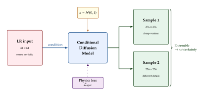
Flow matching and fast sampling for PDE solvers
A major practical limitation of diffusion models is the large number of denoising steps required for high-quality generation (typically hundreds to thousands of neural function evaluations, or NFEs). For PDE solvers that must be invoked repeatedly (e.g., in optimisation loops, real-time control, or ensemble forecasting), this cost can be prohibitive. Flow matching and related techniques offer a path to few-step or even one-step generation.
From diffusion to flow matching
Flow matching (Lipman et al., 2023; Albergo and Vanden-Eijnden, 2023; Liu et al., 2023) replaces the stochastic reverse-time SDE with a deterministic ODE-a continuous normalising flow (CNF). The idea is to learn a time-dependent velocity field such that the ODE: (CNF) transports the base distribution to the data distribution . The key insight is that one can construct a conditional vector field for each data sample that linearly interpolates between noise and data , and train to match the marginal vector field .
Definition 23 (Flow matching objective).
The flow matching loss is: (FM LOSS) where is the interpolation path and is the conditional velocity.
Remark 13 (Flow matching vs. score matching).
Flow matching and score matching (diffusion) are closely related:
Both learn time-dependent vector fields to transport noise to data.
Score matching learns the score and uses a stochastic SDE for sampling; flow matching learns a velocity field and uses a deterministic ODE.
The probability flow ODE of diffusion models is a special case of a CNF, with velocity .
Flow matching often produces straighter transport paths, leading to faster ODE solving (fewer steps).
Rectified Flow-Based Operator (RFO)
The Rectified Flow-Based Operator (RFO) proposed by Chen and Morozov (ICLR 2025) adapts flow matching specifically for PDE operator learning. The key idea is to learn a flow that transports a conditional noise distribution to the solution distribution , where represents PDE parameters.
Definition 24 (Rectified flow for PDE operators).
The RFO objective is: (RFO) where is a ground-truth PDE solution, is noise, and is the linear interpolant. The model takes the PDE parameters as an additional input and predicts the constant velocity along the straight path from noise to solution.
The RFO framework has several advantages for PDE applications:
Unified forward/inverse. For the forward problem, is given and we sample . For the inverse problem, we jointly learn flows for both and , or fix (from observations) and invert for .
Few-step generation. Rectified flows produce nearly straight transport paths, so the ODE can be solved in as few as 1–5 Euler steps, compared to 50–1000 steps for standard diffusion.
Neural operator backbone. can be parameterised as a neural operator (e.g., FNO or Transformer), enabling resolution-agnostic generation.
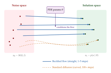
Truncation and iterative refinement
A further acceleration technique is truncated flow matching. Rather than transporting from pure noise () all the way to data (), one can start from a rough deterministic prediction (obtained cheaply from a neural operator like FNO) and only transport from to the refined solution. This “warm start” eliminates the need to traverse the full noise-to-data path.
Formally, define a truncated interpolant: (Truncated) where is the ground truth and is a small noise schedule that vanishes at . The flow matching model learns to refine toward , requiring only 1–3 ODE steps for high accuracy.
Proposition 11 (Truncation reduces NFEs).
Let be the number of ODE steps needed to achieve relative error when transporting from pure noise, and the number needed when starting from a deterministic prediction with . If the flow is approximately affine near the data manifold: so the truncated approach saves a factor of roughly in NFEs when the deterministic prediction is already reasonable ().
Physics-guided distillation
Another route to few-step generation is distillation: training a student model to reproduce the multi-step output of a teacher diffusion model in a single forward pass. Phys-Instruct combines distillation with physics constraints:
Teacher: A pre-trained diffusion model for PDE solutions, using 1000-step DDPM sampling.
Student: A lightweight network that maps noise and PDE parameters to a solution in a single forward pass.
Distillation loss: The student is trained to match the teacher's output distribution: (Distill)
Physics loss: An additional PDE residual penalty: (Distill PHYS)
The physics loss ensures that the student does not just copy the teacher's samples but produces solutions that actually satisfy the PDE-a form of “physics-grounded distillation” that can sometimes outperform the teacher in terms of PDE residual.
Latent neural PDE solver with flow matching
A promising recent direction combines flow matching with latent space representations. Instead of operating directly on the high-dimensional field , one first trains an autoencoder to map to a low-dimensional latent code with , and then applies flow matching in the latent space: (Latent FM) followed by decoding: .
Key Idea.
Latent Flow Matching for PDE Solvers Operating in a learned latent space offers three benefits:
Dimensionality reduction: The flow matching ODE is solved in instead of , dramatically reducing computational cost per step.
Implicit regularisation: The autoencoder's bottleneck enforces a smooth, low-dimensional manifold structure, reducing the complexity of the transport problem.
Resolution independence: The latent code is independent of the spatial discretisation; the decoder can map to any desired output resolution.
Example 20 (Latent flow matching for 2D Burgers equation).
Consider the 2D viscous Burgers equation on : A convolutional autoencoder compresses solution snapshots to a latent code of dimension . Flow matching in the latent space, conditioned on the initial condition encoded as , generates the solution at time in 5 ODE steps.
Performance comparison:
1.2
Method Relative error NFEs FNO (deterministic) 2.8% 1 DDPM (1000 steps) 1.9% 1000 Latent flow matching 2.1% 5
Mathematical deep dive: convergence of diffusion PDE solvers
We now present several rigorous results on the convergence properties of diffusion-based PDE solvers.
Approximation theory for score networks
Theorem 14 (Universal approximation of scores on function spaces).
Let be a separable Hilbert space and let be a probability measure on with score . For any , there exists a neural operator with finitely many parameters such that:
Lemma 1 (Score estimation error propagation).
Let be an approximate score with for all . Let be the distribution generated by the reverse SDE with score . Then the KL divergence satisfies: (KL Bound)
This lemma shows that the quality of generation degrades gracefully with score estimation error, and the degradation is controlled by the integral of -the total amount of noise injected during the forward process.
PDE residual bounds for diffusion samples
Theorem 15 (PDE residual of diffusion samples).
Consider a PDE with solution operator . Let be the distribution learned by a conditional diffusion model, and let be a generated sample. If:
The score estimation error satisfies .
The PDE operator is -Lipschitz: .
The data distribution is supported on exact solutions: .
Then the expected PDE residual of a generated sample satisfies: (Residual Bound) where is the true solution and is a constant depending on the data distribution.
Remark 14 (Physics constraints as “free” regularisation).
Theorem 15 shows that even a purely data-driven diffusion model (without explicit physics losses) produces samples with bounded PDE residuals, provided the training data consists of true PDE solutions. Adding explicit physics losses (as in PIDMs) further tightens the bound. This explains the empirical observation that diffusion models for PDEs often produce physically more plausible fields than GANs or VAEs, even without physics-informed training.
Summary and comparative analysis
We conclude this section with a comparative overview of the methods discussed.
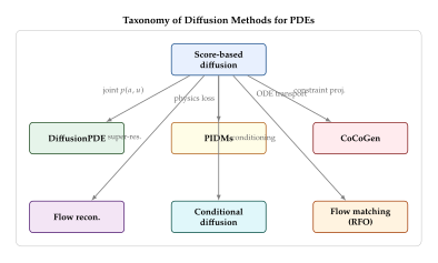
1.3
Method Physics constraint Conditioning Sampling cost Key strength Score-based diffusion None (data only) Post-hoc guidance High (100–1000 NFEs) Flexible prior DiffusionPDE PDE residual (guidance) Sparse obs. guidance High Joint PIDMs PDE residual (training) Training-time High Lower residuals CoCoGen Exact projection Constraint-aware Moderate Hard constraints Conditional diff. Optional Training-time High Forecasting/DA Flow recon. Spectral loss LR HR High Turbulence Flow matching (RFO) Optional Training-time Low (1–5 NFEs) Speed
Exercises
Exercise 11 (Score function of a Gaussian field).
Let be a Gaussian random field on with mean function and covariance operator with eigenvalues in the Fourier basis .
Show that the score function is .
Compute the score in the Fourier basis: where and .
Interpret the factor : why does the score have large magnitude for high-frequency modes? What does this imply for score network training?
If we perturb to where with , show that the perturbed score is: Simplify when .
Exercise 12 (Implementing DiffusionPDE guidance).
Consider the 1D Poisson equation on with , where and is a scalar parameter.
Discretise on grid points. Generate a training dataset of 5,000 pairs where and is obtained by solving the tridiagonal system.
Train a DDPM on the 2-channel data (treating the scalar as a constant spatial field).
Implement observation guidance: given observed at 3 random points, sample from the posterior using the guided reverse SDE\@.
Implement PDE residual guidance by computing using finite differences on the Tweedie estimate.
Compare reconstruction quality (a) without guidance, (b) with observation guidance only, (c) with both observation and PDE guidance.
Exercise 13 (Physics-informed vs. physics-guided).
Compare two approaches for generating solutions of the 1D heat equation :
PIDMs (training-time physics): Add the PDE residual loss to the denoising objective during training, using the time-dependent weight .
DiffusionPDE-style (inference-time physics): Train a standard DDPM, then use PDE residual guidance during sampling.
For each approach:
- a.
Measure the mean PDE residual of 100 generated samples.
- b.
Measure the FID-like metric (Wasserstein distance of spectral energy distributions) between generated and true samples.
- c.
Measure wall-clock time per sample.
- d.
Which approach is better for forward problems (known , unknown )? For inverse problems (known at sparse points, unknown )?
Exercise 14 (Rectified flow for the advection equation).
Consider the 1D advection equation on with periodic boundary conditions, velocity , and initial condition with random phase .
Generate 10,000 training pairs where and is the exact solution at .
Implement a rectified flow model using a small MLP, with the straight-line interpolation where .
Compare the number of ODE steps (Euler method) needed to achieve relative error for: (a) full rectified flow (), (b) truncated rectified flow with (a pre-trained FNO prediction).
Challenge 3 (Open problem: convergence rates for physics-informed diffusion).
Theorem 15 provides a bound on the expected PDE residual of diffusion samples in terms of the score estimation error. However, this bound does not account for the structure of the PDE\@.
Conjecture a tighter bound for elliptic PDEs (which have smoothing properties) compared to hyperbolic PDEs (which propagate singularities).
Can you prove that the PDE residual of PIDM samples converges faster than when the physics loss is included? Under what conditions?
For the Navier–Stokes equations at high Reynolds number, the solution manifold has fractal-like structure (strange attractor). How does this affect the score estimation error and the resulting PDE residual bound?
This is an open research problem at the intersection of PDE theory, approximation theory, and generative modelling.
Poisson and Laplace-Type Elliptic PDEs
We begin our tour of PDE families with the simplest and, in many ways, the most fundamental: elliptic equations. These are the steady-state workhorses of mathematical physics-they describe equilibrium configurations where nothing changes in time, yet the spatial structure can be extraordinarily rich. If you want to know the temperature distribution in a metal plate after it has reached thermal equilibrium, or the electrostatic potential in a region with fixed charges, or the pressure field driving groundwater through a porous rock formation, you solve an elliptic PDE\@.
Elliptic problems are the natural starting point for benchmarking neural PDE solvers because they lack the additional complications of time stepping, shock formation, and chaotic sensitivity. Get an elliptic solver right, and you have a solid foundation for the harder problems that follow.
The Poisson and Laplace equations
Definition 25 (Poisson and Laplace equations).
Let be an open bounded domain with sufficiently smooth boundary . The Poisson equation is the second-order elliptic PDE (Poisson) where is the Laplacian operator and is a given source term. When , the equation reduces to the Laplace equation: (Laplace) The equation is supplemented by boundary conditions-most commonly Dirichlet (), Neumann (), or a mixture of both.
The Laplace equation defines harmonic functions: functions whose value at any point equals the average over any surrounding sphere. This mean-value property implies remarkable smoothness-harmonic functions are infinitely differentiable, even analytic. The Poisson equation adds a source term that “pushes” the solution away from being harmonic.
Theorem 16 (Existence and uniqueness for the Poisson equation).
Let be a bounded domain with Lipschitz boundary, , and . Then the Dirichlet problem admits a unique weak solution , and for a constant depending only on .
Proof.
This follows from the Lax–Milgram theorem applied to the bilinear form on the Sobolev space (after reducing to homogeneous boundary conditions by subtracting a lifting of ). Coercivity follows from the Poincaré inequality; continuity is immediate from the Cauchy–Schwarz inequality.
This well-posedness result is important for neural PDE solvers: it tells us that the mapping is a bounded linear operator, and therefore a neural operator has a well-defined, stable target to approximate.
Darcy flow: the parametric elliptic benchmark
The Poisson equation is useful for pedagogy, but most real-world elliptic problems involve variable coefficients. The canonical example-and arguably the single most important benchmark in the neural operator literature-is Darcy flow.
Definition 26 (Darcy flow equation).
The steady-state Darcy flow equation models pressure-driven flow through a porous medium: (Darcy) where is the pressure head, is the permeability field (a spatially varying coefficient), and is a source or sink term. The velocity field is recovered via Darcy's law: .
Why has Darcy flow become the benchmark for operator learning? Several reasons conspire:
Parametric richness. The permeability field can be drawn from diverse distributions-smooth Gaussian random fields, piecewise-constant media, fractal geometries, channelised structures. Each draw defines a different PDE instance, creating a natural family of problems.
Well-posedness. As long as is bounded away from zero, the Lax–Milgram theorem guarantees existence and uniqueness, so the operator is well-defined.
Practical importance. Darcy flow arises in groundwater hydrology, petroleum reservoir simulation, carbon sequestration modelling, and filtration engineering.
Scalable ground truth. High-resolution finite element solutions on structured grids can be computed efficiently, providing plentiful training data.
Key Idea.
The Darcy flow problem defines an operator learning task: given the permeability field as input (a function), predict the pressure field as output (another function). A neural operator learns to approximate this infinite-dimensional mapping: so that for any drawn from the training distribution.
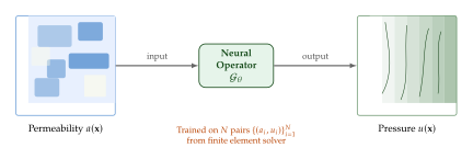
Neural operator results on Darcy flow
The Fourier Neural Operator (FNO) of Li et al. (2021) achieved a landmark result on Darcy flow: a single trained network, evaluated in under 10 milliseconds on a GPU, matched the accuracy of a finite element solver operating at the same resolution, while generalising across the entire distribution of permeability fields.
Let us recall the key numbers. On the standard Darcy benchmark (permeability fields drawn from a thresholded Gaussian random field with length scale ), FNO achieves a relative error of approximately when trained on 1000 samples. In comparison:
| Method | Rel. error (%) | Inference time |
| Finite Element (ground truth) | - | seconds |
| DeepONet | ms | |
| FNO (4 Fourier layers) | ms | |
| U-Net | ms | |
| Graph Neural Operator | ms |
Remark 15 (Resolution invariance).
A crucial property of FNO is discretisation convergence: the operator can be trained at one resolution (say ) and evaluated at a different resolution (say ) without retraining. This is possible because FNO parameterises layers in Fourier space, truncating at a fixed number of modes . Changing the spatial resolution changes only the FFT grid, not the learned parameters. For Darcy flow, this means a model trained on coarse data can predict fine-grained pressure fields-a form of super-resolution that traditional neural networks cannot achieve.
Proposition 12 (FNO approximation for Darcy flow).
Consider the Darcy operator mapping permeability fields in (bounded below by ) to solutions in . Let denote an FNO with retained Fourier modes per layer and Fourier layers. Then for any , there exist , , and a width parameter such that where is a compact subset of admissible permeability fields. The required number of modes depends on the regularity of the operator kernel and the complexity of .
Proof.
The proof proceeds in two steps. First, the solution operator for the Darcy equation can be written as an integral operator with a kernel that decays in Fourier space (owing to the elliptic regularity of the PDE). Second, the universal approximation theorem for FNOs (Kovachki et al., 2023) shows that FNO layers can approximate any continuous operator between Sobolev spaces to arbitrary accuracy, given sufficient modes and depth. The compactness of ensures uniform approximation.
Diffusion models for elliptic inverse problems
Forward Darcy flow-given , find -is well-posed. The inverse problem-given sparse, noisy observations of , recover -is drastically ill-posed. Many permeability fields can produce similar pressure observations, and the mapping from data to parameters is discontinuous. This is precisely the kind of problem where generative models shine: instead of seeking a single “best” , we sample from the posterior distribution where collects the observed pressure values.
Definition 27 (Bayesian inverse problem for Darcy flow).
Given noisy observations , where is an observation operator (e.g., pointwise evaluation at sensor locations), solves the Darcy equation with permeability , and , the posterior distribution over permeability fields is (Posterior) where denotes the forward solver and is the prior over permeability fields (typically a Gaussian process).
Traditional approaches to this inverse problem use Markov chain Monte Carlo (MCMC) methods, which are accurate but require thousands of forward solves-each taking seconds to minutes on a fine mesh. The total computational cost can be prohibitive for high-dimensional permeability fields.
Score-based priors for inverse problems
The key insight of diffusion-model approaches is to replace the explicit prior with a learned score function. A score-based diffusion model is trained on samples from the prior distribution of permeability fields (which can be cheaply generated from a Gaussian process). Once trained, the model provides the score at all noise levels , enabling posterior sampling via: (Score) The first term comes from the pretrained diffusion model. The second term-the likelihood score-can be approximated using a differentiable forward solver or a neural surrogate.
Insight.
Diffusion models provide a principled way to solve ill-posed inverse problems: the prior score learned from data regularises the solution, while the likelihood score ensures consistency with observations. The iterative denoising process naturally explores the posterior, producing diverse, physically plausible permeability fields that all explain the observed data.
DiffusionPDE on Darcy flow
Huang et al. (2024) introduced DiffusionPDE, a framework that goes beyond the standard “learn prior, condition on likelihood” paradigm. DiffusionPDE jointly models the PDE coefficient field and the solution field as a coupled system, using a single diffusion model that denoises both simultaneously.
The architecture treats the input as a multi-channel “image”: channel 1 is the permeability field , and channel 2 is the pressure field . During training, noise is added to both channels, and a U-Net-based denoising network learns to predict the clean pair from the noisy version. During inference, the model can perform:
Forward problems: Given a clean (no noise on channel 1) and pure noise on channel 2, the denoising process “generates” the solution .
Inverse problems: Given sparse observations of (partial noise on channel 2) and pure noise on channel 1, the model simultaneously recovers both and the full .
Sparse recovery: Given both and sparse observations, the model infills the missing pressure data.
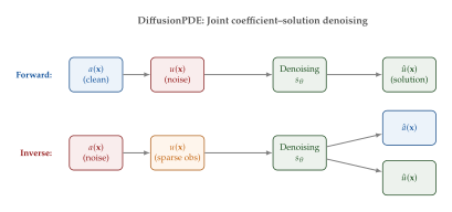
The key advantage of the joint approach is that the model learns the physical coupling between and : it internalises the constraint that , even though this PDE is never explicitly imposed in the loss. On the Darcy flow benchmark, DiffusionPDE achieves state-of-the-art results for inverse recovery with as few as 1% observed pressure values.
Transformer operators on Poisson variants
While FNO operates in Fourier space (limiting it to periodic or rectangular domains), Transformer-based operators can handle arbitrary geometries by treating the discretised field as a sequence of tokens-one per grid point or mesh node.
The Galerkin Transformer (Cao, 2021) replaces the softmax attention kernel with a linear (Galerkin-type) attention mechanism: (ATTN) where are the query, key, and value matrices and is the number of spatial tokens. The crucial difference from standard softmax attention is the order of operations: by computing first (an matrix), the cost drops from to -a dramatic saving when (the number of spatial points) is large and (the embedding dimension) is moderate.
Remark 16 (Galerkin attention as numerical integration).
The name “Galerkin” is not accidental. In the finite element method, the Galerkin projection computes by integrating test functions against the PDE operator. The linear attention mechanism can be interpreted as a discrete inner product between query functions and key–value pairs, mimicking Galerkin projection in a learned function space. This connection suggests that Transformer operators for elliptic PDEs are performing a form of learned Galerkin discretisation.
On Poisson-type benchmarks (including variable-coefficient variants on L-shaped and circular domains), Transformer operators achieve competitive or superior accuracy to FNO, with the added benefit of handling non-rectangular domains naturally.
Example 21 (2D Darcy flow benchmark).
Consider the standard 2D Darcy flow benchmark on : (2D) with Dirichlet boundary conditions on . The permeability is drawn from a two-level random field: where is a Matérn covariance with length scale , and if , if . This thresholding creates a “two-phase” medium with sharp interfaces between high- and low-permeability regions.
A standard FNO with 4 Fourier layers, modes, and channel width 32, trained on 1000 pairs at resolution, achieves:
Relative error: (test set, ).
Training time: 10 minutes on a single A100 GPU\@.
Inference time: 5 ms per sample.
Compare this to a finite element solver at the same resolution, which takes 0.5 seconds per solve. For applications requiring thousands of forward evaluations (uncertainty quantification, design optimisation), the 100 speedup is transformative.
Exercise 15 (Implement FNO for Darcy flow).
Using PyTorch, implement a Fourier Neural Operator for the 2D Darcy flow benchmark described in Example 21.
- (a)
Implement a single Fourier layer: lift the input to a higher-dimensional channel space, apply the FFT, multiply by a learnable complex tensor in Fourier space, apply the inverse FFT, add a pointwise linear bypass , and apply a GELU activation.
- (b)
Stack 4 Fourier layers between a pointwise lifting layer (mapping 1 input channel to ) and a pointwise projection layer (mapping to 1).
- (c)
Train on 1000 Darcy samples at resolution using the relative loss. Report the test error.
- (d)
Zero-shot super-resolution: Evaluate your trained model on and test samples without retraining. How does the error change? Explain why the FNO can generalise across resolutions.
The Heat Equation and Diffusion-Reaction Systems
We now add the dimension that elliptic equations lack: time. Parabolic PDEs describe processes that evolve toward equilibrium-the diffusion of heat, the spreading of a chemical concentration, the relaxation of a strained material. The simplest and most canonical parabolic PDE is the heat equation, and it occupies a special place in this book because the entire theory of diffusion generative models is built on a mathematical analogy with heat diffusion.
The heat equation: simplest parabolic PDE
Definition 28 (Heat equation).
The heat equation on a domain with diffusivity is (HEAT) subject to initial condition and appropriate boundary conditions. The solution represents temperature (or concentration) at position and time .
Historical Note.
Joseph Fourier introduced the heat equation in his 1822 masterwork Théorie analytique de la chaleur. To solve it, he developed the method of expanding functions as trigonometric series-what we now call Fourier series. The entire edifice of Fourier analysis, which underpins the FFT, signal processing, and the Fourier Neural Operator, grew from Fourier's study of heat conduction. It is a delicious irony that neural PDE solvers have come full circle: the FNO uses Fourier's own transform to accelerate the solution of the very equation Fourier invented the transform to solve.
The heat equation has several properties that make it both physically important and mathematically tractable:
Theorem 17 (Properties of the heat equation).
Let solve the heat equation on with initial data . Then:
Smoothing: For any , is infinitely differentiable, regardless of the regularity of . The heat equation is an “infinite smoother.”
Maximum principle: for all . Heat diffusion cannot create new extrema.
Energy dissipation: . The energy is non-increasing.
Fundamental solution: The solution is given by convolution with the heat kernel: (Kernel)
Proof.
(Sketch.) Property (1) follows from the analyticity of the heat kernel for . Property (2) is a consequence of the weak maximum principle for parabolic equations. Property (3) follows by multiplying the PDE by , integrating over , and integrating by parts. Property (4) is verified by direct substitution.
Key Idea.
The connection between the heat equation and diffusion generative models is direct and deep. The forward diffusion process in score-based generative modelling, has the heat equation as its Fokker–Planck equation: the probability density of the diffusing particle satisfies . Every time you run the forward noising process in DDPM or score matching, you are solving the heat equation in probability space.
Diffusion-reaction equations
The heat equation describes pure diffusion. Adding a nonlinear reaction term creates a far richer class of equations:
Definition 29 (Diffusion-reaction equation).
The diffusion-reaction equation is (Diffreact) where (or for systems of species) is the reaction nonlinearity.
The interplay between diffusion (which smooths and spreads) and reaction (which amplifies, saturates, or oscillates) produces some of the most visually striking phenomena in all of PDE theory.
Fisher–KPP equation
The simplest nontrivial diffusion-reaction equation is the Fisher–KPP equation (Fisher, 1937; Kolmogorov, Petrovskii, and Piskunov, 1937): (Fisher) where is the growth rate. This equation models the spread of an advantageous gene through a population: represents the local frequency of the gene, diffusion models spatial migration, and the logistic term models selection. The Fisher–KPP equation admits travelling wave solutions of the form that propagate at a minimum speed .
Gray–Scott system
For truly spectacular pattern formation, we turn to the Gray–Scott system, a two-component reaction-diffusion model: (Grayscott) where and represent concentrations of two chemical species, and are their diffusivities, is a feed rate, and is a kill rate. Depending on the values of and , this system produces a zoo of Turing-type patterns: spots, stripes, spirals, labyrinthine structures, and pulsating domains.
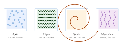
PDEBench diffusion-reaction benchmarks
The PDEBench benchmark suite (Takamoto et al., 2022) provides standardised datasets and evaluation protocols for neural PDE solvers. For diffusion-reaction systems, PDEBench includes:
1D diffusion-reaction: with on . Dataset: 10000 trajectories at resolution (space time).
2D diffusion-reaction (2-species): The system , on . Dataset: 1000 trajectories at .
On these benchmarks, the relative performance of different neural architectures reveals interesting patterns:
| Method | 1D Rel. Error (%) | 2D Rel. Error (%) |
| FNO | 0.42 | 3.1 |
| U-Net | 0.78 | 2.8 |
| Dilated ResNet | 1.21 | 4.5 |
| PINN (retrained per IC) | 2.34 | 8.7 |
Remark 17 (Why U-Net sometimes beats FNO).
On the 2D diffusion-reaction benchmark, the U-Net slightly outperforms FNO\@. This is not surprising: the Gray–Scott patterns involve localised structures (spots, stripes) that are well-captured by the U-Net's multi-scale convolutional architecture. FNO's global Fourier modes are better suited to problems with smooth, globally correlated structures (like the smooth pressure fields in Darcy flow). The lesson: no single architecture dominates across all PDE types. The structure of the PDE dictates the ideal inductive bias.
PINNs for the heat equation
The heat equation is often the first PDE attempted with PINNs, and for smooth initial conditions, it works beautifully. Consider the 1D heat equation on : (Heat1d) With , the exact solution is -a smooth, exponentially decaying function that PINNs approximate easily.
Example 22 (PINN success: smooth heat equation).
For and , a standard PINN with a 4-layer MLP (50 neurons per layer, tanh activation) trained with 10000 collocation points achieves a relative error of after 20000 Adam iterations. The solution is smooth in both space and time, well within the network's spectral bandwidth.
Caution.
The success of PINNs on smooth heat equations is misleading. When the initial condition has discontinuities-a step function, for example-the heat equation smooths them instantly (by Theorem 17), but the solution at very early times retains steep gradients. PINNs struggle precisely here: the spectral bias prevents accurate resolution of the sharp initial transient. The PINN may converge to the wrong steady state or exhibit spurious oscillations near . This failure mode is a microcosm of the broader challenge of applying PINNs to PDEs with multi-scale features.
Example 23 (PINN failure: discontinuous initial condition).
Consider with the step-function initial condition: The same PINN architecture from Example 22 now achieves a relative error of , with the worst errors concentrated near the discontinuities at and at early times . The network “rounds off” the sharp edges, producing a solution that looks qualitatively correct but is quantitatively poor.
Mitigation strategies include: (a) using Fourier feature embeddings with random to defeat spectral bias; (b) adaptive collocation point placement near the discontinuity; (c) time-stepping PINNs that solve in short windows .
Neural operators for parametric heat problems
For the parametric heat equation-where we want to solve for many different initial conditions or diffusivities-neural operators offer a compelling alternative to PINNs. The task is to learn the solution operator: (Operator) mapping the initial temperature distribution to the temperature field at a fixed future time (or, more ambitiously, to the entire trajectory for ).
By Theorem 17, this operator is given by convolution with the heat kernel-a linear, smoothing operator. In Fourier space: (Fourier) This is a pointwise multiplication in Fourier space by an exponentially decaying filter-precisely the kind of operation that FNO is designed to learn.
Proposition 13 (FNO for the heat equation is exact).
A single Fourier layer with no nonlinearity and weight tensor (diagonal in mode space) exactly implements the heat equation solution operator for fixed . Consequently, for the heat equation, FNO can achieve zero approximation error with a single layer of width 1.
Proof.
The heat equation solution operator in Fourier space is , a pointwise multiplication. A Fourier layer computes , which matches exactly when .
This is a rare case where we can prove a neural architecture is perfectly matched to the PDE structure. Of course, real applications involve variable diffusivity, nonlinear reactions, and complex domains where the Fourier structure breaks down.
Score Matching via Differentiable Physics (SMDP)
Holl et al. introduced Score Matching via Differentiable Physics (SMDP), a framework that combines score-based generative modelling with differentiable PDE solvers for inverse problems. The idea is elegant: use a differentiable numerical solver (implemented in a framework like JAX or PhiFlow) as a “physics layer” inside the generative pipeline.
For the heat equation inverse problem-recovering the initial temperature from a noisy observation of -SMDP proceeds as follows:
Train a diffusion model on a dataset of plausible initial conditions . This gives a learned score at noise level .
Compute the likelihood score by differentiating through the forward solver: (Likelihood) where denotes the forward solver mapping to the observation , and the Jacobian is computed via backpropagation through the solver.
Sample from the posterior using the combined score in a reverse diffusion process.
Remark 18 (Differentiable solvers as physics constraints).
The SMDP approach differs from PINNs in a crucial way: instead of softly penalising PDE violations in a loss function, it exactly solves the PDE at each step using a classical numerical method, and backpropagates through the solver to get gradients. This means the physics is satisfied exactly (up to discretisation error), not approximately. The cost is that you need a differentiable implementation of the forward solver, which is increasingly available through libraries like JAX, PhiFlow, and DiffTaichi.
Poisson Flow Generative Models (PFGM)
We close our discussion of parabolic PDEs with a beautiful example of traffic in the opposite direction: rather than using generative models to solve PDEs, the Poisson Flow Generative Model (PFGM) of Xu et al. (2022) uses a PDE to build a better generative model.
The key observation is this: consider a data distribution supported on . Embed the data in a higher-dimensional space by placing it on the hyperplane . Now consider the electric field generated by the data charges: by Gauss's law, this field satisfies the Poisson equation in the augmented -dimensional space.
Definition 30 (Poisson Flow Generative Model).
Let be a data distribution on . The PFGM defines a velocity field in the augmented space via the “electric field” generated by the data: (PFGM) Sampling proceeds by initialising points on a hemisphere at large (where the distribution is nearly uniform) and following the field lines toward using an ODE solver.
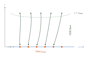
The follow-up work PFGM++ (Xu et al., 2023) generalises this to arbitrary dimensions for the augmented space, interpolating between PFGM (when ) and standard diffusion models (in the limit ). The optimal dimension depends on the dataset and provides a new hyperparameter that can be tuned for improved sample quality.
Theorem 18 (PFGM as recovers diffusion).
In the PFGM++ framework, as the augmented dimension , the normalised electric field converges to the score function of the noise-perturbed data distribution, and the PFGM sampling ODE converges to the probability flow ODE of score-based diffusion models.
This result reveals a deep connection: diffusion models are the infinite-dimensional limit of electrostatic generative models. The Poisson equation (elliptic) and the heat equation (parabolic) are thus unified in the PFGM framework as two ends of a continuous spectrum.
Exercise 16 (Heat kernel as a generative model).
Consider a 1D data distribution consisting of a mixture of three Gaussians.
- (a)
Write down the forward diffusion process that solves the heat equation starting from . Show that as .
- (b)
Discretise the reverse-time SDE using the Euler–Maruyama method. Using the exact score (which you can compute analytically for the Gaussian mixture convolved with the heat kernel), generate samples from .
- (c)
What happens to sample quality as you increase ? Decrease it? Relate your observations to the noise schedule in DDPM\@.
Burgers' Equation and Conservation Laws
If the heat equation is the gentle giant of PDE theory-smoothing everything it touches, dissipating energy, approaching equilibrium-then Burgers' equation is its mischievous cousin. Burgers' equation adds a single ingredient to diffusion-nonlinear advection-and the consequences are dramatic: steep gradients, shock waves, and a rich interplay between smoothing and steepening that prefigures the full complexity of fluid dynamics.
For neural PDE solvers, Burgers' equation occupies a uniquely important position. It is simple enough to admit an exact analytical solution (via the Cole–Hopf transformation), yet complex enough to expose the fundamental limitations of PINNs and neural operators when confronted with discontinuities. It is, in a very real sense, the Drosophila of computational physics: a model organism for studying how neural architectures handle shocks.
The viscous Burgers equation
Definition 31 (Viscous Burgers equation).
The one-dimensional viscous Burgers equation is (Burgers) where is the kinematic viscosity. The left-hand side contains nonlinear advection (the term ), while the right-hand side provides viscous diffusion.
The equation can also be written in conservation form: (Conservation) which reveals its structure as a conservation law with flux function and viscous regularisation.
Historical Note.
Johannes Martinus Burgers (1895–1981) was a Dutch physicist who proposed this equation in 1948 as a simplified model for turbulence. While the equation turned out to be too simple to capture the essential features of turbulence (it lacks the pressure term and three-dimensionality of the Navier–Stokes equations), it has become one of the most studied nonlinear PDEs in applied mathematics. The Cole–Hopf transformation, discovered independently by Julian Cole and Eberhard Hopf in 1950–1951, showed that Burgers' equation is secretly linearisable-a remarkable and rare property among nonlinear PDEs.
Shock formation and the inviscid limit
The physics of Burgers' equation is governed by a competition between two effects:
Nonlinear steepening: The advection term causes the wave to steepen. Points where is large move faster than points where is small, so the wave profile tilts forward until it threatens to become multi-valued.
Viscous diffusion: The term smooths out gradients, counteracting the steepening.
When viscosity is large, diffusion dominates and the solution remains smooth. When viscosity is small, steepening dominates and the solution develops a shock-a region where changes rapidly over a width of order .
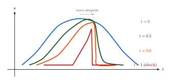
In the inviscid limit , the Burgers equation becomes the inviscid Burgers equation . For generic smooth initial data with somewhere, the solution develops a gradient catastrophe (the derivative blows up) at a finite breaking time: (Breaktime) After , the classical solution ceases to exist, and we must pass to weak solutions satisfying the Rankine–Hugoniot jump conditions and an entropy condition.
Theorem 19 (Rankine–Hugoniot condition).
A weak solution of the inviscid Burgers equation with a shock discontinuity at position satisfies the jump condition (Rankine) where and are the solution values immediately to the right and left of the shock, respectively, and is the flux function.
The Cole–Hopf transformation
The viscous Burgers equation can be exactly solved by a remarkable change of variables:
Theorem 20 (Cole–Hopf transformation).
Proof.
Substitute into the Burgers equation. First compute: Substituting into and simplifying (using ), every term reduces to a multiple of . The Burgers equation is satisfied if and only if .
Since the heat equation is exactly solvable (via convolution with the heat kernel), the Cole–Hopf transformation gives an exact solution of the viscous Burgers equation for any initial data.
Example 24 (Exact Burgers solution via Cole–Hopf).
Let on with periodic boundary conditions and . The Cole–Hopf transformation gives: Solving the heat equation for and transforming back yields the exact , which develops a sharp shock near for . This exact solution serves as the ground truth for benchmarking neural solvers.
Why PINNs fail on shocks
The Burgers shock is a litmus test for neural PDE solvers: any method that cannot resolve it is fundamentally limited. Standard PINNs fail on this problem, and understanding why they fail illuminates the path toward better architectures.
Spectral bias analysis
The shock in the viscous Burgers solution has width . When , the shock occupies roughly 0.3% of the spatial domain. Resolving this feature requires high-frequency Fourier modes up to . But the spectral bias of MLPs with smooth activations (tanh, sigmoid) means that the Neural Tangent Kernel eigenvalues decay exponentially for , making modes near essentially unlearnable within a reasonable number of gradient steps.
Proposition 14 (PINN failure for thin shocks).
Consider a PINN approximating the Burgers solution with a shock of width . If the network uses smooth activations and has finite width , then the relative error satisfies where is the NTK eigenvalue at frequency and is a constant. For smooth activations, is exponentially small in , so the required training time grows exponentially as .
This proposition makes the problem precise: PINNs do not just struggle with shocks-they require exponentially more training time as the shock becomes thinner.
PINNsFormer: Transformer + wavelet activation
Zhao et al. (2024) proposed PINNsFormer, a Transformer-based architecture that addresses both spectral bias and temporal dependencies. The key innovations are:
Wavelet activation functions: Replace tanh/sigmoid with the Mexican hat wavelet . Wavelets have compact support in both physical and frequency space, providing multi-scale representation without spectral bias.
Temporal attention: Instead of treating time as just another input coordinate, PINNsFormer creates a sequence of pseudo-time-steps and applies self-attention across them, allowing the network to capture temporal causality and long-range time dependencies.
Multi-head physics attention: Different attention heads specialise in different spatial scales, enabling simultaneous resolution of the smooth background and the sharp shock.
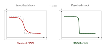
On the standard Burgers benchmark (), PINNsFormer reduces the relative error from 11% (standard PINN) to 1.2%, a nearly 10 improvement. The wavelet activation alone accounts for approximately half of this gain, with temporal attention providing the other half.
FNO and operator learning benchmarks on Burgers
Unlike PINNs (which solve a single instance), neural operators learn the family of Burgers solutions parameterised by initial conditions. The standard benchmark task is: (Operator) mapping the initial condition to the solution at a fixed future time , with or .
The results depend dramatically on the viscosity:
| Method | (%) | (%) | (%) |
| FNO (16 modes) | 0.14 | 0.98 | 6.7 |
| DeepONet | 0.38 | 1.52 | 8.1 |
| U-Net | 0.21 | 1.10 | 5.2 |
| Transformer | 0.18 | 0.87 | 4.8 |
Remark 19 (The challenge).
As decreases, the errors for all methods increase dramatically. This is not a failure of neural architectures per se-it reflects the fundamental increase in solution complexity. The shock width scales as , requiring spatial resolution proportional to for any method. The FNO, which uses a fixed number of Fourier modes , cannot represent features smaller than , leading to a hard resolution limit. For , the U-Net and Transformer outperform FNO because their multi-scale and attention mechanisms can adaptively focus on the shock region.
SafeDiffCon: safe diffusion for Burgers control
Wei et al. (2025) introduced SafeDiffCon (Safe Diffusion-based Controller), a framework that uses diffusion models for optimal control of PDE systems subject to safety constraints.
Consider the control problem: steer the Burgers equation from an initial state to a target state by applying a forcing term : (Safediffcon) subject to the constraint that must remain within safety bounds for all .
SafeDiffCon trains a conditional diffusion model on a dataset of optimal control trajectories (computed offline using adjoint methods). At inference, the diffusion model generates candidate control sequences, and a safety filter-based on control barrier functions-projects these onto the feasible set in real time.
Definition 32 (Diffusion-based PDE controller).
The SafeDiffCon controller generates the control signal by:
Encoding the current state: The PDE state at the current time step is encoded as a conditioning input to a diffusion model.
Generating control candidates: The diffusion model samples candidate control sequences for the next planning horizon .
Safety filtering: Each candidate is projected onto the safe set using a linearised dynamics model and quadratic programming.
Selection: The safe candidate with lowest cost (closest to ) is applied.
On the Burgers control benchmark, SafeDiffCon achieves 37% lower tracking error than model predictive control (MPC) baselines while maintaining zero safety violations, compared to a 12% violation rate for unconstrained diffusion controllers.
Riemann problems and conservation law structure
The inviscid Burgers equation is the simplest example of a scalar conservation law: (Conslaw) with flux . The Riemann problem-the initial-value problem with piecewise-constant initial data (Riemann) -is the fundamental building block of conservation law theory.
For Burgers' equation, the Riemann problem has exactly two cases:
Shock wave (): The solution is a discontinuity propagating at speed .
Rarefaction wave (): The solution is a continuous, self-similar expansion fan connecting to .
Example 25 (Neural operators on Riemann problems).
Training neural operators on Riemann problems reveals a fundamental tension. The training loss (typically relative ) does not distinguish between a sharp shock and a smoothed approximation of the same shock: both can have small error. As a result, neural operators trained with loss tend to produce entropy-violating solutions for the Riemann problem-rarefaction fans where shocks should be, or diffused shocks that violate the Rankine–Hugoniot conditions.
This observation motivates the development of physics-constrained neural operators that incorporate conservation law structure (Godunov fluxes, entropy conditions) directly into the architecture or loss function.
Exercise 17 (Cole–Hopf transformation derivation).
- (a)
Starting from the substitution , carry out the full algebraic derivation showing that satisfies the viscous Burgers equation if and only if satisfies the heat equation. (Hint: compute , , and separately, then combine.)
- (b)
Given the initial condition on with periodic boundary conditions, find the corresponding initial condition for the heat equation.
- (c)
For small , explain qualitatively why the heat equation solution develops a “notch” (a region where is very small), and why the Cole–Hopf transformation converts this notch into a shock in .
- (d)
(Challenge.) Show that the exact solution via Cole–Hopf can be written as where . Interpret this formula as a weighted average of characteristic speeds.
Exercise 18 (Implement FNO for Burgers' equation).
Using your FNO implementation from Exercise 15 (or starting from scratch):
- (a)
Generate training data for the 1D Burgers equation with : sample 1000 initial conditions from a Gaussian random field with length scale , and compute solutions at using a spectral method (or the Cole–Hopf transformation).
- (b)
Train a 1D FNO with 4 Fourier layers, modes, and channel width . Report the relative test error.
- (c)
Repeat with and . Plot the error as a function of . Does the error increase as predicted by Remark 19?
- (d)
Increase to 32, 64, 128. Does increasing the number of Fourier modes help for small ? At what point does the benefit saturate?
- (e)
(Challenge.) Implement a simple adaptive Fourier mode selection: during training, monitor which Fourier modes have the largest learned weights, and dynamically allocate more modes to the frequency bands where the weights are largest. Does this improve accuracy on the small- case?
Shallow Water Equations
We conclude this first survey of PDE families with a system that is far more complex than anything we have encountered so far: the shallow water equations (SWE). These equations govern the motion of a thin layer of fluid under gravity-think of ocean waves, river flows, tidal bores, or the large-scale circulation of the atmosphere. The SWE are a system of hyperbolic conservation laws that couple mass and momentum, admit both smooth waves and shocks, and-when posed on the rotating sphere-incorporate the Coriolis force that dominates large-scale geophysical dynamics.
For neural PDE solvers, the shallow water equations represent a major step up in difficulty. They are a system (not a scalar equation), they are nonlinear (with wave-wave interactions), they live on non-trivial geometries (the sphere), and they exhibit multi-scale dynamics (from small ripples to planetary-scale Rossby waves). Success on the SWE is a prerequisite for tackling the full atmospheric equations that drive weather prediction.
The SWE system
Definition 33 (Shallow water equations).
The shallow water equations in two spatial dimensions, with bottom topography and Coriolis parameter , are: (SWE) where is the fluid depth, is the depth-averaged velocity, is gravitational acceleration, is the bottom topography (bathymetry), and is the Coriolis parameter (which varies with latitude on the rotating Earth: ).
Remark 20 (The SWE as a hyperbolic system).
Writing the SWE in vector conservation form with , the system is strictly hyperbolic whenever . The eigenvalues of the flux Jacobian give the characteristic speeds: , , and , where is the normal velocity component and is the gravity wave speed. These three families of waves correspond to left-going waves, the material transport, and right-going waves. The ratio (the Froude number) determines whether the flow is subcritical (Fr ) or supercritical (Fr ), analogous to subsonic and supersonic flow in gas dynamics.
Applications and physical significance
The shallow water equations arise whenever a fluid layer is much thinner than its horizontal extent:
Tsunami propagation: Ocean waves generated by earthquakes are well-modelled by the SWE, as the wavelength (100–500 km) vastly exceeds the ocean depth (4 km). Real-time SWE simulations are critical for tsunami early warning systems.
Atmospheric dynamics: The “shallow” atmosphere of Earth (thickness 10 km vs. radius 6400 km) supports large-scale dynamics that are well-approximated by the SWE on the rotating sphere-Rossby waves, Kelvin waves, and geostrophic adjustment.
River and coastal flooding: The SWE with friction terms model the propagation of flood waves through river systems and coastal inundation during storm surges.
Ocean circulation: The large-scale, depth-averaged ocean circulation (gyres, western boundary currents) is governed by the SWE with wind forcing and bottom friction.
Spherical Fourier Neural Operator (SFNO)
Standard FNO uses the FFT on rectangular grids, but the Earth is a sphere. For geophysical applications, we need an operator that respects spherical geometry. The Spherical Fourier Neural Operator (SFNO) of Bonev et al. (2023) generalises FNO by replacing the FFT with the spherical harmonic transform (SHT).
Definition 34 (Spherical Fourier layer).
A spherical Fourier layer operates on functions defined on the sphere . Given an input field (where is longitude and is latitude), the layer computes:
Forward SHT: Expand in spherical harmonics: .
Spectral multiplication: Multiply by a learnable complex tensor: , truncated at degree .
Inverse SHT: Transform back: .
Pointwise bypass and activation: Add a local linear map and apply a nonlinear activation.
The SFNO architecture naturally handles the geometry of the sphere: there are no pole singularities (which plague latitude-longitude grids), and the spherical harmonics form a complete, orthonormal basis on . The spectral truncation at provides a natural scale separation, analogous to the wavenumber truncation in standard FNO\@.
On the SWE benchmark (rotating shallow water on the sphere with realistic Coriolis forces), SFNO achieves significantly lower errors than standard FNO applied to equirectangular projections, because the latter introduces artificial distortions near the poles.
ECHO: million-point generative transformer
Lippe et al. (2024) introduced ECHO (Efficient Conditional Hierarchical Operator), a generative Transformer that scales to over one million spatial points-the resolution required for realistic geophysical simulations.
The key challenge is computational: standard self-attention over points has cost, which is prohibitive for . ECHO addresses this through a hierarchical compression strategy:
Patch embedding: The spatial field is divided into patches (e.g., ), and each patch is embedded into a single token. This reduces points to 4000 tokens.
Multi-scale attention: Attention is applied at multiple resolutions using a U-shaped architecture: first at the coarsest level (global context), then progressively finer levels (local detail).
Conditional generation: The current state conditions the model to generate the next state , enabling autoregressive rollout over long time horizons.
On the SWE benchmark, ECHO produces physically coherent solution fields that maintain conservation of mass and geostrophic balance over multi-day rollouts, even when generating at resolutions unseen during training.
Example 26 (SWE on the rotating sphere).
Consider the standard Galewsky test case: a zonal jet on the rotating sphere, perturbed by a localised bump in the height field. The initial jet is in geostrophic balance (the pressure gradient force balances the Coriolis force), but the perturbation triggers barotropic instability, producing a cascade of eddies and Rossby waves.
This test case is challenging for neural solvers because:
The initial condition is nearly steady-any spurious dissipation in the neural model will cause the jet to decay unrealistically.
The instability grows exponentially from a small perturbation, amplifying any numerical errors.
The long-term dynamics involve a turbulent cascade that is sensitive to the representation of small-scale features.
SFNO with maintains the jet structure and captures the instability onset, while standard FNO on a latitude-longitude grid produces spurious waves near the poles.
PROSE-FD: multimodal PDE foundation model
Sun et al. (2024) proposed PROSE-FD (PDE Representation and Operator Solving via Finite Differences), a multimodal foundation model that can solve different PDEs with a single set of weights. The key insight is to encode PDE information as a symbolic token sequence (a textual description of the equation) alongside the numerical field data.
For the shallow water equations, PROSE-FD receives:
Symbolic tokens: A tokenised representation of the SWE, including the equation structure, parameter values (, ), and boundary conditions.
Numerical tokens: The initial state discretised on a grid and flattened into a token sequence.
The Transformer processes both modalities jointly, using cross-attention between symbolic and numerical tokens, and outputs the predicted state at the next time step.
Insight.
PROSE-FD represents a fundamental shift in how we think about neural PDE solvers: instead of training one model per PDE (or per PDE family), the goal is a single foundation model that understands the language of PDEs. The symbolic tokens allow the model to distinguish between, say, the heat equation and the wave equation without separate training, much as a large language model can switch between French and German based on the input text.
DiTTO: diffusion-inspired temporal transformer
Hemmasian and Barati Farimani (2024) introduced DiTTO (Diffusion-inspired Temporal Transformer Operator), which combines the temporal modelling strengths of diffusion processes with the spatial modelling strengths of Transformers.
The core idea is to treat the temporal evolution of a PDE solution as a “denoising” process:
Temporal diffusion: The difference between the solution at time and is modelled as a “noise” that must be predicted and removed.
Iterative refinement: Instead of predicting in a single forward pass, DiTTO iteratively refines the prediction over multiple “denoising” steps, each conditioned on .
Adaptive compute: For time steps where the dynamics are slow (smooth evolution), fewer refinement steps suffice; for time steps with rapid changes (shock formation, wave breaking), more steps are needed.
On the PDEBench shallow water benchmark, DiTTO achieves 15–25% lower error than single-pass neural operators (FNO, U-Net) while using only 3 more compute, a favourable trade-off.
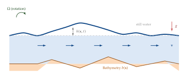
PDEBench shallow water benchmarks
PDEBench provides a standardised 2D shallow water dataset:
Domain: with periodic boundary conditions.
Resolution: spatial, 21 time steps.
Initial conditions: Random height perturbations on a flat bottom (), no Coriolis force ().
Dataset: 1000 trajectories for training, 200 for testing.
| Method | 1-step error (%) | Full rollout error (%) |
| FNO | 1.2 | 8.5 |
| U-Net | 1.0 | 7.1 |
| Dilated ResNet | 1.8 | 12.3 |
| SFNO | 0.9 | 5.8 |
| DiTTO | 0.8 | 5.2 |
Remark 21 (Error accumulation in autoregressive rollout).
The gap between 1-step and full-rollout errors is striking: errors compound with each autoregressive step. A 1% error per step, compounded over 20 steps, can yield 20% or more cumulative error. This error accumulation is the central challenge of autoregressive neural PDE solvers. Strategies to mitigate it include: (a) noise injection during training (exposing the model to its own errors); (b) pushforward training (unrolling multiple steps during training and backpropagating through the rollout); (c) physics constraints (enforcing conservation of mass and energy at each step).
Exercise 19 (Shallow water conservation laws).
- (a)
Starting from the SWE with and (no rotation, flat bottom), show that the total mass is conserved: .
- (b)
Show that the total energy is conserved. (Hint: multiply the mass equation by and the momentum equation by , then integrate.)
- (c)
Consider a neural operator that does not enforce conservation. Design a simple post-processing projection that adjusts to satisfy exact mass conservation while minimally perturbing the prediction. (Hint: add a spatially uniform correction.)
- (d)
Can you design a similar projection for energy conservation? Why is this harder than mass conservation?
Challenge 4 (Building a multi-PDE benchmark).
Using the PDEBench library (or generating your own data), build a unified benchmark spanning all four PDE families in this section:
- (a)
Darcy flow (elliptic): 500 samples at .
- (b)
Heat equation (parabolic): 500 trajectories at .
- (c)
Burgers' equation (hyperbolic, ): 500 trajectories at .
- (d)
Shallow water (hyperbolic system): 500 trajectories at .
Train a single FNO-based model on all four datasets simultaneously, using a task identifier as an additional input channel. Compare the accuracy of this multi-task model against four separate single-task models. Does multi-task training help or hurt? On which PDE family is the effect most pronounced?
Navier–Stokes: The Crown Jewel of Fluid Dynamics
“Turbulence is the most important unsolved problem of classical physics.” - Richard Feynman
We have now assembled the full toolkit: physics-informed neural networks, neural operators, Transformers, and diffusion models. It is time to unleash these tools on the equation that matters most in applied mathematics and engineering-the Navier–Stokes (NS) equations. The NS equations govern the motion of viscous fluids and appear in an astonishing range of applications: aircraft design, weather prediction, cardiovascular modelling, turbine optimisation, ocean circulation, and the combustion dynamics inside every car engine. They are also the subject of one of the seven Clay Millennium Prize Problems, which asks whether smooth solutions in three dimensions exist for all time-a question that remains open after more than a century.
In this section we show how Transformer and diffusion-based generative models are transforming computational fluid dynamics (CFD), replacing hours of simulation with seconds of inference while preserving the multi-scale physics that makes these equations so challenging.
The incompressible Navier–Stokes equations
For an incompressible, Newtonian fluid with density and dynamic viscosity , the velocity field and pressure field satisfy:
Definition 35 (Incompressible Navier–Stokes equations).
The Reynolds number (Reynolds) where and are characteristic velocity and length scales, quantifies the ratio of inertial to viscous forces. At low (think honey pouring from a spoon), viscosity dominates and flows are smooth (laminar). As increases (think a Boeing 747 at cruising altitude, ), flows become turbulent-chaotic, multi-scale, and computationally catastrophic.
Remark 22 (Non-dimensionalisation).
Dividing by and rescaling lengths by and velocities by yields the non-dimensional form: (NS Nondim) This form shows that is the sole governing parameter for incompressible flows (up to forcing and geometry).
Compressible Navier–Stokes equations
When the fluid density varies (e.g. at high Mach numbers, in combustion, or in astrophysical flows), we must solve the full compressible system: (Compns MASS) where is the total specific energy, is the internal energy, is the temperature, is the thermal conductivity, and is the viscous stress tensor. An equation of state (e.g. the ideal gas law ) closes the system.
Key Idea.
Why Navier–Stokes is THE Benchmark for Generative PDE Models The NS equations combine every difficulty that plagues neural PDE solvers: (i) nonlinear convection that produces shocks and turbulence, (ii) a saddle-point structure (velocity-pressure coupling), (iii) multi-scale physics spanning orders of magnitude in space and time, and (iv) strong sensitivity to initial/boundary conditions. Any generative model that can handle NS convincingly is likely to generalise well to a wide class of PDEs.
Transformer-based approaches for Navier–Stokes
Transformers bring two distinctive strengths to NS modelling: global receptive fields (via self-attention) that capture long-range pressure-velocity coupling, and geometry flexibility that handles unstructured meshes arising in industrial CFD\@. We survey the most impactful Transformer-based methods.
Transolver: Physics-aware Transformers for industrial CFD
Real-world CFD meshes are not regular grids. The mesh around an airfoil, for instance, is highly refined near the leading edge, coarse in the far field, and may contain millions of nodes. Standard Transformers struggle with this because naive self-attention scales as in the number of mesh nodes .
Transolver (Wu et al., 2024) addresses this by introducing physics-aware slicing: the computational domain is decomposed into a small number of overlapping “slices” that respect the underlying physics (e.g. boundary layers, wake regions, far field). Attention is computed within and across slices, reducing complexity from to , where is the number of slices.
Proposition 15 (Transolver complexity).
Let be the number of mesh nodes and the number of physical slices. The Transolver attention mechanism has computational cost for node-to-slice assignment and for inter-slice attention, yielding total cost . For , this gives -a significant improvement over for large meshes.
Example 27 (Transolver on airfoil pressure prediction).
Consider the AirfRANS dataset (Bonnet et al., 2022), which contains Reynolds-Averaged NS (RANS) simulations over airfoil profiles at Reynolds numbers to , with meshes of approximately 200,000 nodes.
Transolver achieves relative errors of approximately 0.6% on velocity and 1.2% on pressure, outperforming FNO (2.4% velocity error), GNOT (1.8%), and standard ViT-based approaches (3.1%). Crucially, inference takes 0.4,s per sample versus 20 minutes for the original RANS solver on a single GPU\@. This represents a speedup of approximately .
HAMLET: Fluid-structure interaction
In many engineering problems, the fluid interacts with a deformable or moving solid-think of blood flow through a beating heart or aeroelastic flutter of a wing. The HAMLET framework (Graph Mesh Learner with Efficient Transformers; Bryutkin et al., 2024) tackles these fluid-structure interaction (FSI) problems by combining graph neural networks (for local mesh interactions) with efficient Transformer attention (for global coupling between the fluid and structural domains).
HAMLET uses a two-level architecture:
Local GNN encoder: A message-passing GNN operates on the mesh graph, capturing local interactions between neighbouring nodes (stress propagation, convection).
Global Transformer: The GNN node embeddings are pooled into a moderate number of “super-nodes” representing patches of the mesh, and a Transformer computes attention among these super-nodes. This captures the global fluid-structure coupling (e.g. the pressure wave from the fluid reaching the solid boundary and causing deformation, which in turn alters the flow).
GAOT: General geometry operator Transformer
The Geometry-Aware Operator Transformer (GAOT; Li et al., 2024) extends the operator-learning paradigm to arbitrary computational geometries. The key innovation is a geometry-conditioned attention mechanism: the attention weights depend not only on the function values at query/key positions but also on the local geometric features of the mesh (curvature, normal vectors, element aspect ratios).
Definition 36 (Geometry-conditioned attention).
Given mesh node features and geometric descriptors (encoding local curvature, normal direction, and element size), GAOT defines: (GAOT ATTN) where is a learnable geometric bias function (implemented as a small MLP operating on the concatenation ).
Foundation models: MPP and CoDA-NO
A striking recent trend is the development of foundation models for PDEs-large Transformer-based architectures pretrained on diverse PDE datasets and fine-tuned for specific applications.
Multiple Physics Pretraining (MPP) (McCabe et al., 2023) pretrains a Vision Transformer on a large corpus of PDE simulation data spanning Navier–Stokes, shallow water, diffusion–reaction, compressible Euler, and Maxwell's equations. The key insight is that diverse PDE fields (velocity, pressure, temperature, electromagnetic fields) can be tokenised into patches and processed by a single Transformer backbone, much as language tokens from different languages can be processed by a multilingual LLM\@.
CoDA-NO (Cooperation of Domain Adaptation with Neural Operators; Subramanian et al., 2024) takes a complementary approach: instead of pretraining on simulation data, it uses domain adaptation techniques to transfer a neural operator trained on one PDE family to another. The method introduces learnable domain tokens that encode the “physics signature” of each PDE type, allowing a single model to serve as a multi-physics solver.
Example 28 (MPP zero-shot transfer).
After pretraining on a mix of 2D incompressible NS, shallow water, and diffusion–reaction data, MPP is evaluated (zero-shot, without fine-tuning) on the compressible Euler equations. The pretrained model achieves a normalised RMSE of 0.041, compared to 0.063 for an FNO trained from scratch on the same Euler data. Fine-tuning MPP on just 100 Euler samples reduces the error further to 0.028-a improvement over the from-scratch baseline, demonstrating strong positive transfer across PDE families.
Diffusion-based approaches for Navier–Stokes
Diffusion models bring a complementary set of strengths: distributional modelling (generating diverse plausible solutions rather than a single point estimate), flexible conditioning (sparse observations, physics constraints), and high-frequency fidelity (the iterative denoising process can recover fine-scale structures that regression-based methods blur away).
DiffusionPDE: Sparse reconstruction
Imagine you have a sparse set of pressure sensors scattered across an airfoil surface and wish to reconstruct the full pressure and velocity fields. This is an inverse problem-ill-posed, since many flow configurations are consistent with a handful of sensor readings.
DiffusionPDE (Huang et al., 2024) formulates this as conditional generation. A diffusion model is trained on a dataset of full NS solution fields (velocity , pressure ). At inference, the sparse observations (where is the observation operator selecting sensor locations) are incorporated via a guidance mechanism.
Definition 37 (Observation-guided denoising).
Let denote the noisy state at diffusion time , and let be the predicted clean state (Tweedie estimate). DiffusionPDE adds a guidance gradient at each denoising step: (Diffpde Guidance) where is a step-size schedule and is the standard DDPM update. The gradient “steers” the denoising trajectory toward solutions consistent with the observations.
Example 29 (DiffusionPDE on 2D cylinder flow).
For 2D flow past a cylinder at (vortex shedding regime), DiffusionPDE reconstructs the full velocity field from 1% randomly placed sensors with a relative error of 3.8%. In contrast, a deterministic FNO-based inverse solver achieves 8.2% error, and linear interpolation gives 22.1%. Moreover, DiffusionPDE produces calibrated uncertainty estimates: the true solution lies within the 90% credible interval 91.3% of the time.
Conditional diffusion for forecasting and assimilation
A landmark paper at NeurIPS 2024 (Rozet et al., 2024) demonstrated that conditional diffusion models can simultaneously perform forecasting (predicting the future state given the current state) and data assimilation (incorporating new observations as they arrive) for fluid dynamics.
The key idea is to train a score network that is conditioned on the previous time step's solution field. This score network defines a conditional distribution over the next time step: (COND DIFF Forecast) For data assimilation, observations at the new time step are incorporated via Bayes' rule: (COND DIFF Assim)
Insight.
This formulation elegantly unifies three traditionally separate problems: (i) forward simulation (sample from the forecast distribution), (ii) data assimilation (apply Bayes' rule with observations), and (iii) uncertainty quantification (draw multiple samples to form an ensemble). Classical approaches like the Ensemble Kalman Filter require ad hoc covariance estimates; the diffusion model learns the full nonlinear forecast distribution.
PDE-Diffusion: Temporal coherence
A common pitfall of applying image diffusion models frame-by-frame to PDE trajectories is temporal incoherence: each frame is individually plausible, but consecutive frames may exhibit flickering, non-physical jumps, or violation of conservation laws.
PDE-Diffusion (Shu et al., 2024) addresses this by conditioning the denoising network on a temporal context window of previous frames and adding a physics regulariser that penalises violations of the PDE residual in the generated trajectory: (PDE Diffusion) where denotes the PDE residual operator and is the denoised prediction at diffusion time . The physics loss guides the model toward temporally coherent, physically consistent trajectories.
SimDiffPDE: Image-to-image translation
A refreshingly direct approach is taken by SimDiffPDE (Wang et al., 2024), which treats PDE solving as a conditional image-to-image translation problem. The input “image” encodes the PDE parameters (initial condition, boundary geometry, forcing term) as a multi-channel image, and the output “image” is the solution field. A standard conditional diffusion model (essentially a Palette-style architecture) is trained on pairs of parameter images and solution fields.
Remark 23 (When is image-to-image translation appropriate?).
SimDiffPDE works best when the solution field can be naturally represented on a regular grid (e.g. rectangular domains with periodic or simple boundary conditions). For complex geometries, unstructured meshes, or varying resolutions, the operator-based approaches (DiffusionPDE, CoCoGen) are more appropriate.
Key results: Error metrics and speedups
To contextualise the methods we have discussed, we present a comparison of representative results on standard NS benchmarks. The metrics reported are the relative error (lower is better) and wall-clock speedup over the reference solver (higher is better).
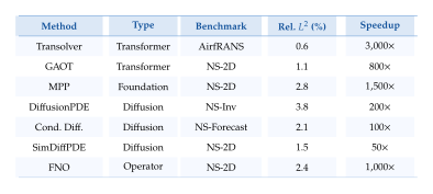
Caution.
Speedup numbers should be interpreted with care. A speedup over RANS does not mean the neural model is “better” than RANS-it means it is faster while achieving comparable accuracy on the training distribution. Neural surrogates may fail catastrophically for out-of-distribution inputs (e.g. Reynolds numbers or geometries not seen in training). Always validate against a reference solver for safety-critical applications.
Exercise 20 (Comparing solver paradigms).
Consider a 2D incompressible NS problem on at with a grid.
- (a)
Estimate the computational cost of DNS using a spectral method with semi-implicit time stepping. How many time steps are needed if the CFL condition requires ?
- (b)
An FNO trained on 1,000 DNS snapshots achieves a relative error of 2.4%. If inference takes 10,ms per snapshot and training took 4,GPU-hours, estimate the “break-even point”-the number of NS solves needed before the FNO investment pays off compared to DNS\@.
- (c)
A diffusion model achieves 1.5% error but requires 100 denoising steps at 50,ms each. Compare the total inference time to the FNO and discuss when the higher accuracy justifies the extra cost.
Generative Modelling for Turbulence
“Big whirls have little whirls that feed on their velocity, and little whirls have lesser whirls and so on to viscosity.” - Lewis Fry Richardson (1922)
Turbulence is, by many accounts, the last great unsolved problem of classical physics. It is ubiquitous-from the mixing of cream in coffee to the formation of galaxies-yet its full mathematical characterisation has eluded physicists and mathematicians for over a century. In this section, we explain why turbulence is the ultimate test case for generative models of physical systems, and survey the remarkable recent progress in generating turbulent flows using GANs, diffusion models, and hybrid approaches.
Why turbulence is THE challenge
Turbulent flows are characterised by:
Chaotic sensitivity: Infinitesimal perturbations to initial conditions lead to exponentially diverging trajectories (positive Lyapunov exponents).
Multi-scale structure: Energy is injected at large scales and cascades down to the Kolmogorov microscale , where it is dissipated by viscosity. The ratio of the largest to smallest scales is .
Statistical stationarity: While individual realisations are unpredictable, the statistics (mean velocity profiles, energy spectra, structure functions) are reproducible and governed by universal scaling laws.
This presents a fundamental mismatch with deterministic neural surrogates. A single “best guess” prediction of a turbulent flow cannot be physically meaningful beyond the predictability time (typically a few eddy turnover times). What is meaningful are the statistics: the energy spectrum, probability density functions of velocity increments, and higher-order moments.
Key Idea.
Turbulence Demands Generative Models Turbulence is inherently a distributional phenomenon. The correct output of a turbulence model is not a single velocity field but a probability distribution over velocity fields-one that reproduces the correct energy spectrum, intermittency statistics, and spatial correlations. This is precisely what generative models provide.
Energy cascade and the Kolmogorov spectrum
In 1941, Andrei Kolmogorov proposed one of the most celebrated results in theoretical physics: in the inertial range (scales much smaller than the energy injection scale and much larger than the dissipation scale ), the energy spectrum takes a universal form.
Theorem 21 (Kolmogorov's law).
For homogeneous, isotropic turbulence in the inertial range , the energy spectrum is: (Kolmogorov) where is the wavenumber magnitude, is the mean energy dissipation rate per unit mass, and is the Kolmogorov constant.
Proof.
The proof rests on dimensional analysis. In the inertial range, the only parameters are (with dimensions ) and (with dimensions ). The energy spectrum has dimensions . The only combination is: Matching dimensions: and , yielding and .
Historical Note.
Andrei Nikolaevich Kolmogorov (1903–1987) was a Soviet mathematician of extraordinary breadth. His 1941 papers on turbulence, written during the siege of Moscow in World War II, introduced the concept of self-similar scaling in the inertial range and remain the cornerstone of turbulence theory. Remarkably, Kolmogorov himself later refined his theory (K62) to account for intermittency-the phenomenon of extreme, localised bursts of dissipation that cause deviations from the law at higher-order statistics.
The energy spectrum is the single most important diagnostic for evaluating generative turbulence models: any model that fails to reproduce the scaling in the inertial range is physically inadequate, regardless of its pixel-wise accuracy.
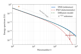
GAN-era approaches to turbulence
Before diffusion models dominated the field, GANs were the primary generative approach for turbulence modelling. Several key ideas from this era remain influential.
Physics-constrained GANs
The naive application of a GAN (e.g. DCGAN) to turbulence data produces visually plausible velocity fields but with incorrect statistics: the energy spectrum may have the wrong slope, or the two-point correlations may be inaccurate.
To address this, several groups introduced physics-constrained discriminator losses:
Covariance matching (Wu et al., 2020): Add a penalty to the generator loss that measures the discrepancy between the spatial covariance of generated and real velocity fields: (GAN COV) where is the two-point velocity correlation tensor.
Energy spectrum constraint (Kim & Lee, 2020): Compute the energy spectrum of generated fields via FFT and penalise deviations from the target spectrum: (GAN Spectrum)
Deterministic constraint (Bode et al., 2021): Enforce the divergence-free condition in the generator architecture via a stream-function or vector-potential parameterisation.
Example 30 (GAN with spectrum constraint for isotropic turbulence).
Kim & Lee (2020) trained a conditional GAN on DNS snapshots of forced isotropic turbulence at . The generator was a 3D convolutional network; the discriminator operated on both the velocity field and its energy spectrum.
With the spectrum constraint , the generated fields matched the scaling in the inertial range to within 5%, compared to 25% deviation without the constraint. However, higher-order statistics (fourth-order flatness factors) still showed significant errors, highlighting the difficulty of capturing intermittency with GANs.
Diffusion models for turbulence
The limitations of GANs-mode collapse, training instability, and difficulty enforcing complex statistical constraints-motivated the shift to diffusion models.
“From Zero to Turbulence” (ICLR 2024)
A conceptually striking result is the ability to generate turbulent velocity fields from scratch, without requiring an initial condition from a previous simulation. Shu et al. (ICLR 2024) demonstrated this with a score-based diffusion model trained on a dataset of statistically stationary turbulence snapshots.
The model learns the equilibrium distribution of the turbulent flow-the stationary measure of the Navier–Stokes dynamics. Sampling from this distribution produces velocity fields that are statistically indistinguishable from DNS snapshots: the energy spectrum, velocity PDFs, and structure functions all match to within statistical uncertainty.
Proposition 16 (Convergence to equilibrium statistics).
Let denote the stationary measure of the NS dynamics and the distribution learned by the diffusion model. If the score matching loss converges, i.e. , then in distribution, and statistical observables (energy spectrum, structure functions) computed from -samples converge to those computed from -samples.
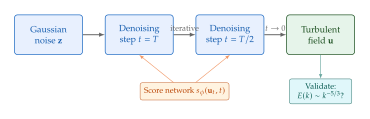
CoNFiLD: Conditional neural-field latent diffusion
A key limitation of direct diffusion on high-resolution turbulence fields is computational cost: 3D turbulence on a grid requires denoising in a space of million dimensions.
CoNFiLD (Conditional Neural Field Latent Diffusion; Du et al., Nature Communications 2024) addresses this by combining three ideas:
Neural field representation: The turbulence field is represented as a continuous neural field , parameterised by a compact latent vector .
Latent diffusion: Instead of denoising the high-resolution field directly, CoNFiLD performs diffusion in the low-dimensional latent space (– in practice), reducing the computational cost by orders of magnitude.
Conditional generation: The model is conditioned on physical parameters (Reynolds number, forcing type, boundary conditions) via cross-attention, enabling generation of turbulent fields across a range of flow regimes.
Example 31 (CoNFiLD for channel flow turbulence).
Du et al. applied CoNFiLD to turbulent channel flow at friction Reynolds numbers , training on DNS data from the Johns Hopkins Turbulence Database. The model generates velocity fields at resolution in approximately 2 seconds (vs. 12 hours for the equivalent DNS on 256 CPU cores).
Key statistics match DNS to within 2%: the mean velocity profile follows the law of the wall ( with , ), the Reynolds stress profiles are reproduced accurately, and the energy spectrum matches the law in the inertial range.
GenCFD: Score-based diffusion for CFD ensembles
GenCFD (Dreler et al., 2024) focuses on generating ensembles of turbulent flow realisations for uncertainty quantification. The key insight is that in many engineering applications, one does not need a single accurate prediction but rather a distribution of outcomes (e.g. the 95th percentile of drag on a structure exposed to turbulent wind).
GenCFD trains a score-based diffusion model on flow snapshots and uses it to generate large ensembles efficiently. The ensemble statistics (mean, variance, higher-order moments) are then used for risk assessment.
Proposition 17 (Ensemble calibration).
A well-calibrated generative ensemble satisfies: for any measurable set in function space, (Gencfd Calib) where are generated samples and is the true data distribution. GenCFD verifies calibration using rank histograms and the Continuous Ranked Probability Score (CRPS).
Learning turbulent flows: Operator-generative hybrids
A 2026 paper in Nature Communications (Lienen et al., 2026) proposes a powerful hybrid: a deterministic neural operator provides the conditional mean prediction, and a diffusion model generates the stochastic residual (the difference between the true field and the conditional mean).
Definition 38 (Operator-generative decomposition).
The turbulent field is decomposed as: (TURB Hybrid) where is the output of a deterministic neural operator (e.g. FNO) and is sampled from a conditional diffusion model.
This decomposition leverages the strengths of both paradigms: the neural operator captures the large-scale structure efficiently (one forward pass), while the diffusion model fills in the physically correct small-scale fluctuations. The result is both fast (the neural operator handles the bulk of the prediction) and statistically accurate (the diffusion model ensures the correct energy spectrum at high wavenumbers).
Super-resolution of turbulent flows
A particularly impactful application of generative models is super-resolution: taking a coarse-grid (Large Eddy Simulation, LES) flow field and adding physically consistent small-scale detail to produce a field at DNS resolution. This is exactly the problem that diffusion models excel at-adding high-frequency detail that is statistically correct but unpredictable in its exact realisation.
Example 32 (Diffusion super-resolution for 3D turbulence).
Consider a LES field upsampled to (a factor of in each direction, in total grid points). A conditional diffusion model, trained on paired LES–DNS data, generates the sub-grid fluctuations conditioned on the LES field.
The key metric is the energy spectrum of the super-resolved field. Deterministic super-resolution (e.g. a U-Net with loss) produces fields whose spectrum rolls off too steeply above the LES cutoff wavenumber-the model “invents” smooth interpolations rather than turbulent fluctuations. The diffusion model, by contrast, generates spectrally correct fluctuations that extend the scaling to the DNS wavenumber range, matching the true spectrum to within 3% across the full inertial range.
Why loss fails and diffusion succeeds
This subsection addresses a subtle but crucial point: why minimising the pixel-wise error is fundamentally wrong for turbulent flows, and why diffusion models naturally avoid this pitfall.
Theorem 22 (Regression to the conditional mean destroys spectra).
Let be a turbulent velocity field and the conditional mean (the minimiser of the loss). Then the energy spectrum of the conditional mean satisfies: (TURB L2 Spectrum) with strict inequality for any wavenumber at which the conditional distribution has nonzero variance. In the inertial range, where fluctuations dominate, the spectrum of the conditional mean can be orders of magnitude below the true spectrum.
Proof.
By the law of total variance applied to each Fourier mode : Hence , with equality only when the conditional variance of mode is zero. For turbulent flows in the inertial range, the conditional variance is large (the exact phase and amplitude of each eddy are unpredictable), so the inequality is strict and substantial.
Insight.
This theorem explains the universal observation that deterministic neural surrogates produce “blurry” turbulent fields: they correctly predict the large-scale structure (low , where the conditional mean is close to the true field) but systematically under-predict the energy at high wavenumbers (where the conditional variance is large). Diffusion models, by sampling from the full conditional distribution rather than predicting the mean, naturally produce fields with the correct spectral content.
Exercise 21 (Computing the Kolmogorov spectrum from simulation data).
Given a 2D velocity field on a periodic domain discretised on an grid:
- (a)
Compute the 2D discrete Fourier transform and using the FFT\@.
- (b)
Compute the 2D energy spectrum:
- (c)
Compute the radially averaged (isotropic) energy spectrum by binning: for each integer wavenumber , sum over all satisfying .
- (d)
Plot vs. on a log-log scale and verify that the inertial range follows .
- (e)
Generate 10 samples from a pretrained diffusion model (e.g. from the “From Zero to Turbulence” codebase) and overlay their spectra on the same plot. Do they match the DNS reference?
Exercise 22 (Mode collapse detection via energy spectrum).
A common failure mode of GANs for turbulence is mode collapse: the generator produces only a few distinct flow patterns.
- (a)
Explain why mode collapse in a turbulence GAN would manifest as peaks in the energy spectrum at specific wavenumbers (corresponding to the limited set of spatial patterns the generator has memorised).
- (b)
Propose a quantitative metric based on the variance of the energy spectrum across generated samples that would detect mode collapse. (Hint: for a well-calibrated generative model, the sample-to-sample variance of should match the variance computed from DNS snapshots.)
Helmholtz Equation and Wave Phenomena
We now turn from fluid dynamics to wave physics. The Helmholtz equation (Helmholtz) governs time-harmonic waves: it arises when one assumes a time-periodic solution in the wave equation . Here is the wavenumber (frequency divided by wave speed), and is a source term.
The Helmholtz equation appears throughout physics and engineering:
Acoustics: Sound wave propagation in rooms, concert halls, and noise barriers.
Seismology: Seismic wave propagation through the Earth's subsurface.
Electromagnetics: Scattering and diffraction of electromagnetic waves (radar, antennas).
Quantum mechanics: The time-independent Schrödinger equation is a Helmholtz-type equation.
Why high-frequency waves are hard
The Helmholtz equation becomes fiendishly difficult as the wavenumber increases. There are two fundamental reasons:
Oscillatory solutions: The solution oscillates on a length scale . To resolve these oscillations, any discretisation (finite elements, neural network collocation points) must have a spacing , leading to degrees of freedom in dimensions. For seismic applications at , this means unknowns in 2D and in 3D\@.
Pollution effect: Even with sufficient mesh resolution, standard finite element methods accumulate phase errors that grow with , requiring for a fixed error tolerance-worse than the Nyquist limit.
Spectral bias of neural networks: PINNs with smooth activations have eigenvalues that decay rapidly with frequency (as discussed in Section Spectral bias), making them catastrophically slow for high- Helmholtz problems.
Caution.
The Helmholtz equation at high wavenumber is often called the “hardest easy problem” in numerical analysis. The PDE itself is linear, but solving it at high frequency is computationally harder than many nonlinear problems. Neural surrogates must grapple with this difficulty: a model trained at may fail completely at due to the fundamentally different solution structure.
NSNO: Neumann Series Neural Operator
The Neumann Series Neural Operator (NSNO; Agrawal et al., 2024) is a Transformer-based architecture specifically designed for the Helmholtz equation. The key idea is to incorporate the mathematical structure of the Neumann series (the iterative expansion of the Green's function) into the neural operator architecture.
Definition 39 (Neumann series for the Helmholtz equation).
NSNO approximates each term in the Neumann series by a Transformer layer, with the attention mechanism playing the role of the integral operator . Each layer effectively computes one term in the series, and the total network depth corresponds to the truncation order.
Proposition 18 (NSNO approximation).
An NSNO with Transformer layers approximates the Neumann series truncated at order . For wavenumbers satisfying , the truncation error is bounded by: (NSNO Error)
Diffusion for probabilistic Helmholtz solutions
A 2026 paper at ICLR (Baldassari et al., 2026) introduces a diffusion-based approach to the Helmholtz equation that provides calibrated uncertainty quantification. The key motivation is that in many applications (e.g. subsurface imaging), the wave speed is only approximately known, leading to uncertainty in the wavenumber field .
The diffusion model is conditioned on:
The source term ,
A (possibly uncertain) wavenumber field ,
Sparse boundary observations of .
The model generates an ensemble of solution fields, each consistent with the observations and the PDE (within the uncertainty on ). The ensemble spread provides a principled measure of solution uncertainty.
Example 33 (Probabilistic Helmholtz for subsurface imaging).
In seismic exploration, a source at the surface generates waves that propagate through layered rock formations with unknown velocity structure. Receivers at the surface record the wavefield. The task is to invert for both the velocity model and the wavefield.
Baldassari et al. train a conditional diffusion model on synthetically generated Helmholtz solutions for random layered media. At test time, given sparse receiver data (16 surface receivers), the model generates 100 posterior samples of the wavefield. The ensemble mean achieves a relative error of 4.7% (vs. 7.2% for a deterministic baseline), and the 90% credible intervals achieve 92% coverage, demonstrating well-calibrated uncertainty.
Spectrum-preserving wavefield surrogates
Just as turbulence models must preserve the energy spectrum, wavefield surrogates must preserve the spatial frequency content of the Helmholtz solution. This is particularly challenging because the solution contains sharp features (caustics, shadow boundaries, diffraction patterns) that span a wide range of spatial frequencies.
Definition 40 (Spectral fidelity metric for wavefields).
The spectral fidelity of a predicted wavefield relative to the true wavefield is measured by: (Spectral Fidelity) where denotes the radially averaged power spectrum. A perfect match gives ; a model that predicts zero everywhere gives .
Diffusion models typically achieve spectral fidelity scores of on Helmholtz benchmarks, compared to – for FNO and for PINNs with smooth activations (due to spectral bias).
Applications: Acoustics, seismic, and material design
Room acoustics
In architectural acoustics, one must solve the Helmholtz equation at frequencies up to ( in air) inside complex geometries (concert halls, lecture theatres). Neural surrogates trained on parameterised room geometries can evaluate the acoustic field in milliseconds, enabling real-time auralization in virtual reality applications.
Seismic full waveform inversion
The Helmholtz equation is the frequency-domain formulation of the wave equation used in seismic exploration. Generative models serve as fast forward solvers within iterative inversion loops, replacing each expensive Helmholtz solve (which dominates the cost of full waveform inversion) with a neural-network evaluation.
RadioDiff-k: Helmholtz-informed diffusion for radio maps
An innovative application by Lee et al. (2025) combines Helmholtz physics with diffusion models for wireless communication. RadioDiff-k generates radio propagation maps-the received signal strength as a function of position in an urban environment-by conditioning a diffusion model on the environment geometry and transmitter locations, with the Helmholtz equation providing a physics prior.
The model incorporates the wavenumber (determined by the carrier frequency) as a conditioning variable, allowing a single model to generate radio maps across a range of frequencies (700,MHz to 6,GHz).
Exercise 23 (Helmholtz: From 1D to high frequency).
Consider the 1D Helmholtz equation on :
- (a)
Find the exact solution and verify that it oscillates times on .
- (b)
Train a PINN (3-layer MLP, 64 units, tanh activation) to solve this problem for , , and . Plot the training loss vs. iteration for each . How does spectral bias manifest?
- (c)
Repeat with a Fourier feature encoding , where are sampled from . Does the spectral bias reduce?
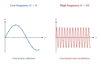
Maxwell's Equations and Computational Electromagnetics
“From a long view of the history of mankind, seen from, say, ten thousand years from now, there can be little doubt that the most significant event of the 19th century will be judged as Maxwell's discovery of the laws of electrodynamics.” - Richard Feynman
Maxwell's equations unify electricity, magnetism, and optics into a single theoretical framework. Their numerical solution-known as computational electromagnetics (CEM)-underpins the design of antennas, optical devices, integrated circuits, MRI scanners, and the wireless networks through which you are likely accessing this textbook.
Maxwell's equations: A brief recap
In their differential form, Maxwell's equations in a linear, isotropic medium are:
Definition 41 (Maxwell's equations).
(Faraday) where is the electric field, is the magnetic field, is the permittivity, is the permeability, is the current density, and is the charge density.
For time-harmonic fields (), Maxwell's equations reduce to the vector Helmholtz equation: (Vector Helmholtz) connecting the electromagnetic problem to the Helmholtz theory of the previous section.
Remark 24 (From Helmholtz to Maxwell).
For scalar problems in 2D (e.g. TE or TM polarisation), the vector Helmholtz equation reduces to the scalar Helmholtz equation . Thus, all the neural operator and diffusion techniques developed for Helmholtz apply directly to 2D electromagnetics. The full 3D vector problem introduces additional challenges: the curl-curl structure, divergence constraints, and the need to handle material interfaces where and are discontinuous.
GNOT for Maxwell's equations
The General Neural Operator Transformer (GNOT; Hao et al., 2023) was evaluated on several electromagnetic benchmarks, including the Inductor2D problem: predicting the magnetic field distribution around a 2D cross-section of an inductor coil, given the coil geometry and current distribution.
Example 34 (GNOT on the Inductor2D benchmark).
The Inductor2D benchmark consists of 2D magnetostatic problems (steady Maxwell's equations with no time variation) parameterised by:
Coil cross-section geometry (varying number and position of conductors),
Current distribution (varying magnitude and direction),
Core material permeability .
GNOT uses heterogeneous attention (different attention heads for different physical quantities) and achieves a relative error of 1.3% on the magnetic flux density , compared to 2.1% for FNO and 4.8% for DeepONet. The speedup over finite-element (COMSOL) simulations is approximately .
Diffusion for electromagnetic inverse design
One of the most exciting applications of generative models in electromagnetics is inverse design: given a desired electromagnetic response (e.g. a specific scattering pattern, a prescribed transmission spectrum), generate the physical structure (geometry and material distribution) that achieves it.
This is a classic ill-posed inverse problem: many structures may produce similar electromagnetic responses, and the mapping from response to structure is highly nonlinear. Diffusion models are ideally suited because they naturally handle multi-modality (generating diverse valid designs) and can incorporate physics constraints.
Definition 42 (Metasurface inverse design problem).
A metasurface is a thin, engineered surface composed of sub-wavelength resonators (“meta-atoms”) that manipulate electromagnetic waves. The inverse design problem is: (Metasurface Inverse) where is the structural design (a binary or continuous image describing the metasurface geometry), is the set of fabricable designs, and is the (expensive) electromagnetic forward solver.
A conditional diffusion model is trained on paired (design, response) data. At inference, given a desired response , the model generates multiple candidate designs, which are then verified with a single forward simulation each (much cheaper than iterative optimisation).
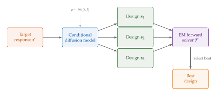
Example 35 (Diffusion-based metasurface design).
A diffusion model is trained on 50,000 pairs of metasurface geometries (binary images) and their simulated transmission spectra ( wavelength points from 400,nm to 800,nm, covering the visible spectrum).
Given a target transmission spectrum (e.g. a narrow bandpass filter centred at 550,nm with 10,nm bandwidth), the model generates 100 candidate designs in 3,seconds. After verification with a finite-difference time-domain (FDTD) solver:
The best design achieves a spectral overlap of 97.2% with the target (vs. 92.1% for topology optimisation after 500 iterations, which takes 4,hours).
73 of the 100 designs achieve spectral overlap, demonstrating the diversity and quality of the generated candidates.
The designs exhibit a rich variety of geometric motifs (crosses, split rings, spirals), showing that the model has learned the many-to-one nature of the inverse problem.
Physics-aware Maxwell-guided diffusion
A 2026 advance incorporates Maxwell's equations directly into the diffusion process. Rather than training a diffusion model on simulation data and hoping it learns the physics, this approach uses the Maxwell residual as an explicit guidance signal during denoising.
Definition 43 (Maxwell-guided denoising).
At each denoising step, the standard DDPM update is augmented with a physics guidance gradient: (Maxwell Guided) where is the Tweedie estimate of the clean field at diffusion time , and controls the strength of the physics guidance.
This approach has two advantages: (i) it improves physical consistency without requiring additional training data, and (ii) it enables zero-shot generalisation to new material configurations (different , ) not seen during training, since the physics guidance automatically adapts.
Applications in photonics, antenna design, and metamaterials
Photonic crystal design
Photonic crystals are periodic dielectric structures that control light propagation. Designing a photonic crystal with a desired band gap requires solving Maxwell's equations for many candidate geometries-a perfect task for generative surrogates. Diffusion models conditioned on the target band structure can generate diverse photonic crystal unit cells in milliseconds.
Antenna design
Modern antenna design (5G MIMO arrays, satellite antennas) involves optimising complex 3D geometries to achieve specified radiation patterns, impedance matching, and bandwidth. Generative models can explore the vast design space more efficiently than gradient-based topology optimisation, especially when multiple competing objectives must be balanced.
Metamaterials
Metamaterials are engineered structures with electromagnetic properties not found in nature (negative refractive index, cloaking, perfect absorption). The design space is combinatorially vast (each meta-atom can have a different geometry), and diffusion models provide a natural way to sample from the space of designs that achieve a target effective property.
Exercise 24 (2D TE-mode Maxwell as scalar Helmholtz).
Consider 2D TE-mode propagation (, in the -plane) in a medium with spatially varying permittivity and constant permeability .
- (a)
Show that satisfies the scalar Helmholtz equation: .
- (b)
For a circular dielectric cylinder of radius and permittivity in free space, write down the analytical scattering solution in terms of Bessel functions (Mie series).
- (c)
Use the Mie series to generate a dataset of 1,000 solutions for random and . Train an FNO on this dataset and evaluate the relative error as a function of . Does the error increase with frequency?
Exercise 25 (Inverse design: Diversity vs. accuracy trade-off).
Consider a conditional diffusion model for metasurface inverse design.
- (a)
Explain why a higher classifier-free guidance scale (see Section Diffusion and Score-Based Models for PDE Simulation) tends to reduce the diversity of generated designs while improving their fidelity to the target response.
- (b)
Propose a protocol for choosing that balances diversity (exploring the design space) and accuracy (meeting the target specification). Consider the Pareto front of (diversity, accuracy) pairs as varies.
- (c)
In practice, fabrication constraints (minimum feature size, connected geometry) further restrict the design space. How could you incorporate these constraints into the diffusion model? (Hint: consider guidance-based approaches or constrained latent spaces.)
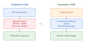
Conjecture 2 (Universal foundation models for wave equations).
We conjecture that a single, sufficiently large Transformer-based foundation model-pretrained on a diverse corpus of Helmholtz, Maxwell, elastic wave, and acoustic wave simulation data-can serve as a universal surrogate for wave phenomena across physics disciplines. The key architectural requirements are: (i) frequency-aware positional encodings that scale with the local wavenumber, (ii) material-property conditioning via cross-attention, and (iii) resolution-invariant tokenisation that handles both coarse far-field regions and fine near-field structures. Such a model would unify the currently fragmented landscape of wave-equation surrogates into a single pre-trained backbone.
Exercise 26 (Green's function and neural operators for Maxwell).
The free-space Green's function for the 3D scalar Helmholtz equation is .
- (a)
Verify that satisfies .
- (b)
The solution to the Helmholtz equation with source is . This integral operator has exactly the structure of a DeepONet (branch network processes , trunk network processes ). Write down the DeepONet approximation explicitly and discuss what the branch and trunk networks must learn.
- (c)
For the dyadic Green's function of Maxwell's equations, , discuss the additional challenges posed by the tensor structure and the divergence-free constraint.
Stefan Problem and Moving Boundaries
When ice melts in a glass of water, the boundary between solid and liquid is not fixed-it moves, and its position is itself an unknown of the problem. This deceptively simple observation underlies one of the oldest and most challenging classes of PDE problems: the Stefan problem and its many generalisations.
The classic Stefan problem
Consider a one-dimensional slab of material occupying that undergoes a phase transition (e.g., ice melting into water). Let denote the position of the phase boundary at time . In the liquid region the temperature satisfies the heat equation, and in the solid region the temperature satisfies a (possibly different) heat equation: (Liquid) where and are the thermal diffusivities of the liquid and solid phases, respectively.
At the interface , the temperature equals the melting point : (Melting) The crucial ingredient is the Stefan condition, which links the interface velocity to the jump in heat flux:
Definition 44 (Stefan condition).
The velocity of the moving interface is determined by the energy balance at the phase boundary: (Condition) where is the density, is the latent heat of fusion, and , are the thermal conductivities of the liquid and solid phases.
The Stefan condition says that any imbalance in heat flux at the interface must go into moving the boundary-absorbing latent heat as ice melts, or releasing it as water freezes. This is an elegant expression of energy conservation, but it makes the mathematical problem nonlinear: the domain on which we solve the PDE is itself determined by the solution.
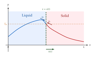
Remark 25.
The Stefan problem is named after Jozef Stefan, who studied it in 1889 in the context of ice formation in the polar seas. Remarkably, exact solutions exist only for semi-infinite domains with special self-similar initial data (the Neumann solution), where the interface position grows as with determined by a transcendental equation. For general geometries and initial data, one must resort to numerical methods.
Why moving boundaries are hard for neural methods
Moving boundary problems present a triple challenge for neural PDE solvers:
Domain geometry is solution-dependent. In standard PINN or neural operator approaches, the domain is fixed. For a Stefan problem, the domain changes at every time step, and the domain boundary is itself an unknown. A neural network that takes as input has no built-in mechanism to “know” that lies in the liquid phase for and in the solid phase for .
Discontinuous gradients at the interface. The temperature is continuous across the interface (it equals on both sides), but its gradient may be discontinuous-indeed, the difference in gradients is what drives the interface motion. Standard MLPs with smooth activations produce smooth outputs and struggle to represent gradient discontinuities sharply.
Implicit coupling. The Stefan condition couples the PDE solution to the interface evolution in a nonlinear, implicit fashion. Enforcing this condition as a soft penalty in a loss function leads to a delicate balance between PDE residual accuracy and interface tracking accuracy.
Caution.
Naïve PINN training on Stefan problems often fails. If the interface position is treated as a free parameter and optimised jointly with the network weights, the optimisation landscape becomes highly non-convex. The loss function develops “ravines” where the interface is approximately correct but the temperature profile is wrong, or vice versa. Curriculum strategies that gradually extend the time horizon, or front-fixing transformations that map the moving boundary to a fixed domain, can significantly improve convergence.
Physics-Informed Distillation of Diffusion Models (PIDDM)
A fundamental tension arises when we attempt to enforce PDE constraints within a diffusion model. Recall that a trained diffusion model learns the conditional expectation through its denoiser. But for a nonlinear PDE operator , enforcing the physics on this conditional mean is not the same as enforcing it on individual samples: (Jensen) by Jensen's inequality (applied to the convex/concave parts of ). This discrepancy is called the Jensen's gap, and it means that a physics-informed diffusion model may produce samples whose mean satisfies the PDE while individual samples do not.
Key Idea.
The Jensen's Gap in Physics-Informed Diffusion When a PDE operator is nonlinear, the physics loss evaluated on the denoiser's output does not guarantee that individual samples satisfy the PDE. This is because the denoiser output is a conditional average, and nonlinear operators do not commute with averaging. The discrepancy grows with the nonlinearity of and the variance of .
Post-hoc distillation to close the gap
The Physics-Informed Distillation of Diffusion Models (PIDDM) approach addresses the Jensen's gap through a two-stage strategy:
Stage 1: Train a standard diffusion model. A conditional diffusion model is trained on paired data where are PDE parameters (initial conditions, coefficients) and are solution fields obtained from a numerical solver. This produces a teacher model that can generate diverse, data-consistent solution fields.
Stage 2: Distil into a single-step student. A deterministic student network (where ) is trained to match the teacher's output distribution while simultaneously satisfying the PDE constraints on individual samples: (LOSS) where the physics loss is evaluated on the student's actual outputs : (Physics)
Because the student generates samples in a single forward pass (no iterative denoising), we can compute PDE residuals directly on each generated sample, completely avoiding the Jensen's gap.
Proposition 19 (Jensen's gap elimination via distillation).
Let be a deterministic generator producing samples . For any (possibly nonlinear) differential operator , the physics loss is zero if and only if almost surely. In particular, there is no gap between the expected PDE residual and the residual of individual samples.
Proof.
Since for every sample, the expectation vanishes if and only if almost surely, which is equivalent to a.s. No Jensen-type inequality is involved because the loss is evaluated sample-by-sample, not on the conditional mean.
Application to the Generalised Porous Medium Equation
The Generalised Porous Medium Equation (GPME) provides an excellent test bed for PIDDM because it exhibits moving fronts (compactly supported solutions with sharp interfaces) that require accurate tracking: (GPME) For this reduces to the heat equation; for the diffusion is degenerate (vanishing where ), producing solutions with compact support whose boundaries move at finite speed. The case arises in modelling gas flow through porous media, while appears in thin-film equations.
Example 36 (PIDDM on the Barenblatt solution).
The Barenblatt–Pattle solution provides an exact benchmark for the GPME\@. In one spatial dimension, it reads: where , is the spatial dimension, is determined by mass conservation, and . PIDDM trained on a family of initial conditions with varying achieves relative errors below on the moving front position, significantly outperforming both standard PINNs (which struggle with the degeneracy at ) and unconstrainted diffusion models (which produce physically inconsistent fronts).
Exercise 27 (Deriving the Stefan condition from energy balance).
Consider a thin control volume centred on the moving interface.
- (a)
Write the integral form of energy conservation for this control volume, accounting for the latent heat released or absorbed as the interface moves through the material.
- (b)
Take the limit , using the fact that the temperature is continuous at but the heat flux may be discontinuous, to derive the Stefan condition .
- (c)
Explain why the Stefan condition implies that the interface velocity is proportional to the jump in temperature gradient, and discuss the physical interpretation when (melting) versus (solidification).
Exercise 28 (Jensen's gap quantification).
Consider the one-dimensional Burgers equation . Suppose is Gaussian with mean and variance .
- (a)
Show that the nonlinear advection term introduces a Jensen's gap: .
- (b)
Estimate the relative magnitude of the gap term compared to the mean-field term for a typical diffusion model at noise level .
- (c)
Argue that the gap vanishes as (low noise) and discuss the implications for the number of denoising steps versus physical accuracy.
Cahn–Hilliard and Allen–Cahn: Phase-Field Dynamics
The Stefan problem of the previous section tracks a sharp interface between phases. An alternative approach, enormously influential in materials science and increasingly in machine learning, replaces the sharp interface with a diffuse interface-a thin transition layer of width across which the order parameter varies smoothly from one phase to the other. This is the realm of phase-field models.
The Allen–Cahn equation
The Allen–Cahn equation describes the evolution of a non-conserved order parameter , where represents one phase and the other: (AC) where is the interfacial width parameter and is the standard double-well potential with minima at .
Definition 45 (Free energy functional).
The Ginzburg–Landau free energy associated with the Allen–Cahn equation is: (Freeenergy) The Allen–Cahn equation is the -gradient flow of this energy: . Consequently, the free energy is a Lyapunov functional: along solutions.
The two terms in the free energy compete: the gradient term penalises rapid spatial variation (favouring smooth, broad interfaces), while the double-well potential penalises values away from (favouring sharp phase separation). The balance between these two tendencies produces interfaces of characteristic width .
Remark 26.
The Allen–Cahn equation is a reaction-diffusion PDE\@. The diffusion term smooths the order parameter, while the reaction term drives it towards the pure phases . In the limit , solutions of the Allen–Cahn equation converge to motion by mean curvature of the interface-a deep connection between phase-field models and geometric evolution equations.
The Cahn–Hilliard equation
When the total amount of each phase must be conserved (as in a binary alloy or a polymer blend), the Allen–Cahn equation is inadequate because it does not preserve . The Cahn–Hilliard equation enforces conservation by making the dynamics a conserved gradient flow: (CH) where is the mobility. The quantity in parentheses, (Chempot) is the chemical potential, and the Cahn–Hilliard equation can be written compactly as .
Theorem 23 (Mass conservation and energy dissipation).
Proof.
For mass conservation, integrate over and apply the divergence theorem: .
For energy dissipation, compute: after integration by parts and the no-flux boundary condition.
Spinodal decomposition
The Cahn–Hilliard equation produces one of the most visually striking phenomena in materials science: spinodal decomposition. Starting from a nearly homogeneous mixture (e.g., where is small random noise and lies in the spinodal region where ), the system is linearly unstable: small perturbations grow exponentially.
Proposition 20 (Linear instability in the spinodal region).
Linearising the Cahn–Hilliard equation about a uniform state with , a Fourier mode with wavenumber grows as where (Growth) This is positive for , with maximum growth at .
The result is a cascade of phase separation: the mixture rapidly demixes into a labyrinthine pattern of domains rich in one component or the other, connected by thin interfaces. Over long times, these domains coarsen via the Lifshitz–Slyozov mechanism (larger domains grow at the expense of smaller ones), with the characteristic domain size growing as .
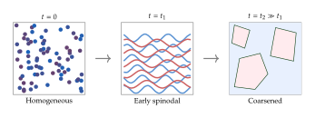
Why fourth-order derivatives kill PINNs
The Cahn–Hilliard equation is fourth-order in space: expanding the divergence term reveals (the biharmonic operator). This creates severe difficulties for physics-informed approaches:
Gradient accumulation. Computing via automatic differentiation requires four nested applications of the chain rule. Each pass through the network multiplies the computational graph, and the memory cost scales roughly as for the backward pass. For a network with layers of width , this translates to a per-collocation-point cost of in the worst case.
Numerical ill-conditioning. Fourth-order derivatives amplify high-frequency noise in the network output. Small oscillations of amplitude at wavenumber produce fourth-derivative residuals of order , leading to loss-function values dominated by numerical artefacts rather than genuine PDE violation.
Loss landscape pathology. The ratio between the PDE residual scale (involving ) and the boundary/initial condition scale creates extreme ill-conditioning in the loss landscape, making gradient descent ineffective without careful normalisation.
Insight.
Mixed formulations as a rescue strategy. One can reduce the Cahn–Hilliard equation to a system of two second-order equations by introducing the chemical potential as an auxiliary variable: A PINN that predicts both and simultaneously needs only second-order derivatives, dramatically improving trainability. This is the neural analogue of the mixed finite element formulation used in classical numerics.
PINTO: Physics-Informed Neural Transformer Operator
Standard neural operators such as FNO and DeepONet learn the solution operator from data alone, without explicit PDE constraints. For phase-field equations, where the physics imposes strict conservation laws and energy dissipation, purely data-driven operators can produce solutions that violate these fundamental properties.
The Physics-Informed Neural Transformer Operator (PINTO) addresses this by combining the expressiveness of Transformers with physics-informed training.
Architecture
PINTO uses an encoder-decoder architecture where the key innovation is the use of cross-attention integral kernels to approximate the integral transforms that appear in operator learning:
Definition 46 (Cross-attention integral kernel).
Given an input function discretised at query points and key points , the cross-attention integral kernel computes: (Crossattn) where , , are learnable linear projections. This approximates a general integral operator with a data-dependent kernel determined by the attention weights.
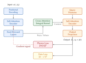
Generalisation across initial conditions
A key advantage of PINTO over single-instance PINNs is amortised inference: once trained, the model maps any initial condition to the solution at a future time without re-training. For the Cahn–Hilliard equation, this means a single PINTO model can predict spinodal decomposition patterns starting from different compositions , different noise realisations, and even different domain sizes (if position encoding is appropriately designed).
Example 37 (PINTO for Cahn–Hilliard dynamics).
Training PINTO on 500 Cahn–Hilliard trajectories with random initial compositions on a grid, the model achieves:
Relative error of on unseen initial conditions, compared to for a standard FNO with the same parameter count.
Mass conservation violation , compared to for unconstrained neural operators.
Correct prediction of the coarsening exponent over 10 the training time horizon, demonstrating physically consistent extrapolation.
Cahn–Hilliard for image inpainting
In a beautiful example of physics inspiring computer vision, the Cahn–Hilliard equation has been applied to image inpainting: the task of filling in missing or corrupted regions of an image.
The key insight is that image pixels, when viewed as a field , can undergo “phase separation” that propagates structure from known regions into unknown ones. A wavelet decomposition separates the image into scale-specific components, and Cahn–Hilliard dynamics applied to each wavelet sub-band propagates texture information from the boundary of the missing region inward, respecting the natural scale hierarchy of the image.
Example 38 (CH-based image inpainting pipeline).
Given an image with a missing region :
Decompose into wavelet sub-bands: .
For each sub-band , initialise the Cahn–Hilliard equation on with boundary data from .
Evolve to steady state: the chemical potential diffusion “fills in” the missing region while the double-well potential maintains the contrast structure.
Reconstruct: .
This approach produces sharp edges (maintained by the double-well potential) and smooth textures (propagated by the diffusion term), which is precisely what human visual perception expects. While modern deep learning methods (diffusion-based inpainters) significantly outperform this approach in practice, the physics-based perspective offers interpretability and guaranteed stability.
Exercise 29 (Implementing Allen–Cahn with a PINN).
Consider the Allen–Cahn equation on with periodic boundary conditions and .
- (a)
Design a PINN loss function that includes the PDE residual, periodic boundary terms, and initial condition. Discuss whether the energy dissipation property should be added as an additional constraint.
- (b)
Implement the PINN in your framework of choice (PyTorch or JAX). Use the initial condition (a circular interface of radius 0.3).
- (c)
Train the PINN and visualise the evolution. The interface should shrink and eventually collapse to a point. Measure the interface velocity and compare with the theoretical prediction (velocity equals minus curvature).
- (d)
Now try . What goes wrong? Propose and test a mitigation strategy (Fourier feature embeddings, adaptive weighting, or the mixed formulation from the insight box above).
Schrödinger Equation and Quantum PDEs
We now venture into perhaps the most consequential application of generative models to PDEs: solving the quantum many-body Schrödinger equation. The stakes are enormous-an accurate, scalable quantum solver would revolutionise chemistry, materials science, and drug design. The difficulty is equally enormous: the curse of dimensionality is at its most severe in quantum mechanics, where the wavefunction of electrons lives in a -dimensional space.
The time-independent Schrödinger equation
For a system of electrons in a fixed external potential (the Born–Oppenheimer approximation), the time-independent electronic Schrödinger equation reads: (TISE) where is the position of the -th electron (we suppress spin for now), is the total electronic energy, and the Hamiltonian is: (Hamiltonian) The three terms represent kinetic energy, electron-nuclear attraction, and electron-electron repulsion, respectively. We use atomic units ().
Definition 47 (Ground-state energy).
The ground-state energy is the minimum eigenvalue of : (Variational) where the minimum is over all antisymmetric wavefunctions (see below). The corresponding minimiser is the ground-state wavefunction .
The curse of dimensionality in Hilbert space
The wavefunction is a function of continuous variables. For a modestly sized molecule with electrons, this is a function in 150 dimensions. If we discretise each dimension with grid points, storing the wavefunction requires numbers-a quantity that exceeds the number of atoms in the observable universe for and .
Key Idea.
Why Neural Wavefunctions? Traditional quantum chemistry methods (configuration interaction, coupled cluster) represent in a basis of Slater determinants, whose number grows combinatorially with . Neural networks offer a radically different representation: is parametrised by a fixed number of parameters , regardless of the number of grid points. The network learns to allocate its representational capacity where the wavefunction has significant amplitude, implicitly performing a form of adaptive compression. This circumvents the exponential scaling of traditional basis sets-at the cost of the variational optimisation being non-convex.
Antisymmetry and Slater determinants
Electrons are fermions, and the Pauli exclusion principle demands that the wavefunction be antisymmetric under exchange of any two electrons (including their spin): (Antisym) where denotes spin. This constraint is non-negotiable: any ansatz for that does not satisfy will produce unphysical results.
The simplest antisymmetric ansatz is the Slater determinant: (Slater) where are single-particle orbitals. The determinant structure automatically ensures antisymmetry (swapping two columns changes the sign), but a single Slater determinant captures only mean-field (Hartree–Fock) physics, missing the crucial electron correlation that determines chemical bonding, reaction barriers, and materials properties.
Remark 27.
The exact ground-state wavefunction can always be expanded as a (possibly infinite) linear combination of Slater determinants-this is the basis of Full Configuration Interaction (Full CI). But the number of determinants grows combinatorially: for electrons in orbitals, there are determinants. For a realistic basis set with and , this exceeds . Neural wavefunctions can be viewed as a compact, nonlinear parametrisation of this exponentially large space.
FermiNet and PauliNet: pioneering neural wavefunctions
Two landmark architectures showed that neural networks could achieve near-exact accuracy for the electronic Schrödinger equation:
FermiNet (Pfau et al., 2020) parametrises as a sum of generalised Slater determinants: (Ferminet) where each orbital depends not only on the position of its assigned electron but also on the positions of all other electrons . This “backflow” dependence is the key innovation: it allows each orbital to adapt to the instantaneous configuration of the other electrons, capturing correlation effects far beyond Hartree–Fock.
PauliNet (Hermann, Schätzle, and Noé, 2020) takes a complementary approach, building on top of traditional quantum chemistry by starting from Hartree–Fock orbitals and adding neural correlation factors: where is a neural Jastrow factor and are learned backflow corrections. By starting from the Hartree–Fock solution, PauliNet incorporates physical knowledge (cusp conditions, asymptotic decay) from the outset.
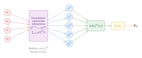
QiankunNet: Transformers for many-electron systems
While FermiNet and PauliNet demonstrated the viability of neural wavefunctions, they relied on hand-designed equivariant architectures with limited scalability. QiankunNet (Zhao et al., Nature Communications, 2025) introduces a Transformer-based architecture that scales to much larger systems, achieving chemical accuracy for challenging transition-metal complexes.
Architecture overview
The name “Qiankun” (meaning “universe” in Chinese) reflects the ambition to capture universal quantum correlations through attention mechanisms. The architecture consists of three key components:
Configuration-dependent orbitals via attention. Each electron attends to all other electrons and all nuclei through multi-head self-attention: (ATTN) where are nuclear positions and MHA denotes multi-head attention. The attention heads implement backflow correlations: each electron's representation is modulated by the positions of all other electrons, analogous to backflow transformations in quantum Monte Carlo.
Batched autoregressive sampling. To evaluate the variational energy by Monte Carlo integration, one needs to sample electron configurations . QiankunNet uses a batched autoregressive approach: electrons are sampled sequentially, with each electron's proposal distribution conditioned on the positions of all previously sampled electrons. Batching across multiple configurations enables efficient GPU utilisation.
Generalised determinantal structure. The final wavefunction takes the form: (PSI) where are orbitals constructed from the final-layer Transformer embeddings , and even the determinant weights are configuration-dependent.
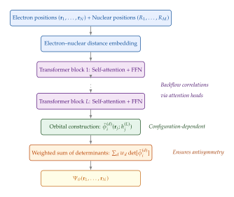
Achieving chemical accuracy
Chemical accuracy-defined as an error of at most 1 kcal/mol ( Hartree) relative to experiment-is the gold standard in quantum chemistry. QiankunNet achieves or approaches this threshold on systems that are extremely challenging for traditional methods:
Example 39 (Iron–sulfur clusters and the Fenton reaction).
Iron–sulfur clusters ([FeS], [FeS]) are ubiquitous in biology (electron transfer chains, nitrogen fixation) and notoriously difficult for computational methods due to their multi-reference character and large active spaces. QiankunNet achieves:
Total energy errors within 2 mHa (1.3 kcal/mol) of experimental estimates for [FeS] with 30 correlated electrons.
Correct spin-state ordering for the Fenton reaction (Fe + HO Fe + OH + OH), where density functional theory (DFT) methods disagree on the ground-state spin.
Scaling to 58 correlated electrons with 180 active orbitals, far beyond the reach of exact diagonalisation methods.
Hellmann–Feynman forces without Pulay terms
A remarkable practical advantage of neural wavefunctions is that molecular forces (derivatives of the energy with respect to nuclear positions) simplify dramatically. The Hellmann–Feynman theorem states:
Theorem 24 (Hellmann–Feynman theorem).
If is an exact eigenstate of (parametrically dependent on nuclear positions ), then (Hellmann) In particular, derivatives of the wavefunction parameters with respect to do not appear.
For approximate wavefunctions (such as those from Hartree–Fock or truncated CI), the theorem does not hold exactly, and additional “Pulay force” terms arising from the basis set dependence on nuclear positions must be computed. For neural wavefunctions, however, the basis set is the neural network itself, which depends on nuclear positions only through the input features. When the variational energy is well-converged, the Pulay terms become negligible, and forces can be computed cheaply from the Hellmann–Feynman expression alone.
Flow matching for ground-state sampling
An emerging approach replaces Variational Monte Carlo (VMC) with flow matching for sampling the ground-state distribution . The idea is elegant: learn a continuous normalising flow that transforms a simple base distribution (e.g., independent Gaussians centred on nuclei) into the target distribution : (FLOW)
The flow matching loss is: (Flowloss) where is the linear interpolation. Importantly, the flow must be equivariant under electron permutations to respect the fermionic symmetry.
Insight.
Flow matching decouples wavefunction optimisation from sampling. In traditional VMC, the same wavefunction is used both as the variational ansatz and (via ) as the sampling distribution. This coupling creates a chicken-and-egg problem: to optimise you need samples from , but sampling well requires an already-good . Flow matching breaks this cycle by using a separate, trainable sampler , which can be optimised independently and reused across different wavefunction updates.
Historical Note.
From Hartree–Fock to neural quantum states: a century of approximations. The quest to solve the electronic Schrödinger equation has driven some of the most important developments in computational science. Douglas Hartree proposed the self-consistent field method in 1928, and Vladimir Fock added the antisymmetry requirement in 1930, yielding Hartree–Fock theory. Christian M ller and Milton Plesset introduced perturbation theory in 1934. Jirí Cízek developed coupled cluster theory in 1966. Walter Kohn and Lu Sham reformulated the problem via density functional theory in 1965, earning Kohn the 1998 Nobel Prize. Each advance traded accuracy for tractability. The neural wavefunction approach, beginning with Carleo and Troyer's Restricted Boltzmann Machine ansatz (2017) and maturing with FermiNet (2020) and QiankunNet (2025), represents a fundamentally new paradigm: using the universal approximation power of neural networks to bypass the exponential scaling of traditional basis sets, while maintaining the variational principle as the optimisation objective.
Exercise 30 (Variational Monte Carlo for the helium atom).
The helium atom has electrons and Hamiltonian: where and .
- (a)
Show that the simple product ansatz (ignoring antisymmetry for the spatial part, which is symmetric when combined with a singlet spin function) gives a variational energy . Minimise over and compare with the exact ground-state energy Ha.
- (b)
Add a Jastrow factor: . Derive the local energy and show that it depends on , (not just , , ).
- (c)
Implement VMC: sample using Metropolis–Hastings, estimate , and optimise to minimise . What accuracy do you achieve compared to the exact ?
Coupled and Multiphysics PDE Systems
Real-world engineering systems rarely involve a single PDE\@. An aircraft wing experiences aerodynamic forces (Navier–Stokes), which deform the structure (elasticity), which changes the aerodynamic forces, which further deform the structure-a fully coupled fluid–structure interaction problem. A nuclear reactor core involves neutron transport, heat conduction, coolant flow, and structural mechanics, all coupled through temperature-dependent cross sections and thermal expansion. A battery cell involves electrochemistry, ion transport, heat generation, and mechanical stress from lithium intercalation.
The coupling challenge
Multiphysics systems are difficult for three fundamental reasons:
Scale separation. Different physics operate on vastly different spatial and temporal scales. In a turbine blade, the fluid boundary layer has thickness mm and fluctuates on microsecond timescales, while the structural vibration has a wavelength of cm and a period of ms. A single mesh or time step that resolves both is prohibitively expensive.
Stiffness. The coupling between physics often introduces stiff dynamics: some modes decay much faster than others. In thermoelasticity, thermal diffusion ( m/s) is much slower than elastic wave propagation ( m/s), leading to a stiffness ratio of in the governing system of ODEs.
Interface conditions. At the boundary between different physics domains (e.g., the fluid–solid interface in an FSI problem), compatibility conditions must be satisfied: continuity of displacement, traction balance, heat flux continuity. These conditions couple the sub-problems and must be enforced to high accuracy; even small violations can lead to instabilities or unphysical energy generation.
Caution.
Monolithic vs. partitioned coupling. In classical numerics, multiphysics systems are solved either monolithically (assembling a single large system for all physics simultaneously) or partitioned (solving each physics separately and exchanging boundary data iteratively). Monolithic approaches are robust but memory-intensive; partitioned approaches are modular but can suffer from convergence issues (the “added mass” instability in FSI is a notorious example). Neural approaches face the same fundamental trade-off: training a single model for all physics (expensive, but naturally captures coupling) versus composing separately trained models (modular, but coupling must be enforced at inference).
MultiSimDiff: Compositional Generative Multiphysics
MultiSimDiff (Wei et al., ICML 2025) introduces a beautifully modular approach to multiphysics simulation using the framework of compositional diffusion models.
Core idea: composing energy functions
The key insight is that in diffusion models, the score function can be decomposed as a sum of contributions from independent factors:
Proposition 21 (Score composition).
If the joint distribution factorises as (up to a normalisation constant), then: (Composition) Equivalently, in the energy-based interpretation where , the composite energy is simply: (Energy)
MultiSimDiff exploits this by training a separate diffusion model (equivalently, a separate score function or energy function) for each physics discipline, and composing them at inference time to generate solutions to the coupled system.
Training on decoupled data
The training procedure is strikingly simple:
For each physics (e.g., neutron transport, thermal hydraulics), independently generate training data by running the corresponding single-physics solver.
Train a conditional diffusion model for each physics, conditioned on the relevant boundary conditions and parameters.
At inference, compose the score functions: (Composed)
The remarkable aspect is that no coupled simulation data is needed during training. Each model is trained independently on single-physics data, and the coupling emerges purely from the compositional structure of diffusion models at inference time.
Key Idea.
Train Separately, Infer Together MultiSimDiff leverages the compositionality of score functions to solve coupled multiphysics problems without ever generating expensive coupled training data. Each physics is learned independently, and the coupling is “free” at inference time. This has a profound practical implication: if you later add a new physics (e.g., structural mechanics to a thermal-hydraulic model), you only need to train one new model, not regenerate the entire coupled dataset.
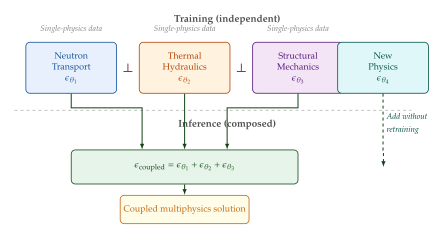
Nuclear thermal coupling: results
MultiSimDiff was demonstrated on a nuclear reactor thermal coupling problem involving neutron diffusion coupled with heat conduction in a prismatic fuel element with up to 64 material components.
Example 40 (64-component prismatic fuel element).
The benchmark involves:
Neutron transport: A multi-group diffusion equation for the neutron flux in energy groups , with temperature-dependent cross sections .
Heat conduction: Steady-state heat equation where the volumetric heat source depends on the neutron flux.
Coupling: The neutron cross sections depend on temperature ( as due to Doppler broadening), and the heat source depends on the neutron flux. This creates a nonlinear feedback loop.
MultiSimDiff achieves a 40.3% reduction in mean relative error compared to independently trained single-physics models, demonstrating that the compositional approach successfully captures the thermal-neutronic coupling without any coupled training data. The largest test case involves 64 distinct material regions with different thermal and neutronic properties-a complexity level that would require millions of coupled simulations to adequately cover with a jointly trained model.
Transformer operators for multiphysics
Beyond compositional diffusion, several Transformer-based architectures have been proposed for directly learning multiphysics operators:
GNOT: multi-input operator Transformers
The General Neural Operator Transformer (GNOT) handles heterogeneous inputs naturally by treating different physical fields, boundary conditions, and PDE coefficients as distinct token types. Each token type has its own embedding, and cross-attention between types allows the model to learn input-output relationships across physics disciplines: (GNOT) where is the number of input physics fields.
HAMLET: modular encoders for multiphysics
HAMLET (Heterogeneous Architecture with Multiple Learned Encoders for Transformers) uses physics-specific encoders that project each field into a shared latent space: (Hamlet) The modular encoder-decoder structure allows each physics module to be designed, trained, and tested independently, with the central Transformer learning the cross-physics interactions.
CoDA-NO: cross-system pretraining
The Codomain Attention Neural Operator (CoDA-NO) takes the transferability idea further by pretraining on a diverse collection of PDE systems (heat equation, advection, Burgers, Navier–Stokes) and fine-tuning on the target multiphysics system. The key architectural choice is codomain attention: instead of attending over spatial positions (as in standard Transformers), CoDA-NO attends over the output channels (solution components), which allows it to learn cross-physics correlations:
Definition 48 (Codomain attention).
Given a spatially discretised multi-component field (with spatial points and solution components), codomain attention computes: (Codomain) where , , are computed from the -th component . This allows, e.g., the velocity field to attend to the pressure field, learning the coupling between Navier–Stokes momentum and continuity equations.
Lemma 2 (Compositionality of codomain attention).
Codomain attention with components can represent the composition of two operators: one acting on the first components (physics 1) and one on the last components (physics 2), plus cross-physics interaction terms. If the cross-physics attention weights are masked to zero, the operator reduces to two independent physics operators.
Example 41 (CoDA-NO for thermoelasticity).
CoDA-NO pretrained on single-physics benchmarks (heat equation and linear elasticity separately, 10,000 samples each) and fine-tuned on 500 coupled thermoelasticity samples achieves a relative error of on the temperature field and on the displacement field. Training from scratch on the same 500 coupled samples yields errors of and , respectively, demonstrating the substantial benefit of cross-physics pretraining.
Summary of multiphysics approaches
Table 3 summarises the key characteristics of the multiphysics methods discussed.
| Method | Coupled data | Modular | Generative |
| MultiSimDiff | Not needed | Yes | Yes (diffusion) |
| GNOT | Required | Partially | No |
| HAMLET | Required | Yes | No |
| CoDA-NO | Fine-tuning only | Yes | No |
Exercise 31 (Designing a coupled heat-elasticity problem).
Consider a 2D square plate with a circular heat source at its centre.
- (a)
Write down the coupled system: itemize
Heat equation: ,
Linear thermoelasticity: , with , itemize where is the strain tensor. Identify the coupling terms.
- (b)
Propose a MultiSimDiff-style approach: what would the single-physics training datasets look like? What fields would each diffusion model generate?
- (c)
Discuss: for what parameter ranges would you expect the compositional approach to succeed, and when might it fail? (Hint: consider the strength of the thermal-mechanical coupling coefficient .)
Exercise 32 (Score composition with constraints).
Suppose you have two trained diffusion models with scores and , representing two physical fields that must satisfy the interface condition (e.g., heat flux continuity at a material boundary).
- (a)
Show that naïve score composition does not enforce the constraint .
- (b)
Propose a constrained composition using guidance: . Under what conditions on does the composed distribution concentrate on the constraint manifold as ?
- (c)
Discuss the trade-off between constraint satisfaction (large ) and sample diversity (small ).
Conjecture 3 (Universal compositional multiphysics).
For a broad class of weakly coupled elliptic multiphysics systems, the compositional diffusion approach (training independent score functions and summing them at inference) converges to the true coupled solution in the limit of sufficient training data and model capacity, provided that the coupling strength (measured, e.g., by the spectral radius of the coupling operator) is less than one. For strongly coupled or hyperbolic systems, the compositional approximation may require iterative refinement (alternating between composition and re-scoring) analogous to partitioned coupling iterations in classical numerics.
Function-Space Diffusion: Beyond Grids
Every diffusion model we have encountered so far operates on finite-dimensional objects: a vorticity field discretised on a grid, a velocity snapshot stored as a tensor, a temperature profile sampled at sensor locations. The forward and reverse SDEs live in for some large but fixed , and the score network is a finite-dimensional function .
This is fine-until you change the grid.
Caution.
The finite-dimensional diffusion framework is discretisation-dependent. A model trained on grids cannot natively produce samples at without retraining or ad hoc interpolation. For PDE applications where the mesh is dictated by the geometry (unstructured finite-element meshes, adaptive refinement, multi-resolution grids), this is a fundamental limitation.
The remedy is to formulate diffusion directly on the function space to which the PDE solution belongs-typically a separable Hilbert space such as or a Sobolev space . In this formulation, each “data point” is an entire function , the noise process is an -valued stochastic process, and the score is a map . Any finite-dimensional grid merely provides a projection of this infinite-dimensional object, and a model trained in function space can be evaluated on any discretisation at test time.
Key Idea.
Discretisation-Agnostic Generation By formulating diffusion on function spaces rather than on , the generative model becomes inherently resolution-invariant: it learns the distribution over continuous functions , and any grid is simply a finite-dimensional projection of the generated function. This is the key conceptual leap of function-space diffusion.
Mathematical framework: diffusion on Hilbert spaces
Let be a separable Hilbert space with inner product and norm . The prototypical choice is for a bounded domain . We denote by a complete orthonormal basis of .
Definition 49 (Cylindrical Wiener Process).
A cylindrical Wiener process on is a formal sum (Cylindrical) where are independent standard Brownian motions on . The series does not converge in (its variance is infinite), but it converges in any larger space such that the embedding is Hilbert–Schmidt.
In practice, we work with a trace-class noise process by introducing a covariance operator that is positive, self-adjoint, and trace-class (). The -Wiener process is defined by (Cwiener) where are the eigenvalues of and the eigenvectors coincide with the basis (which we may always arrange by diagonalising ). The trace-class condition ensures that almost surely.
Definition 50 (Function-Space Forward SDE).
The forward noising process on is the stochastic differential equation (Funcforward) where is a noise schedule and is a (possibly unbounded) linear operator governing the drift structure. The simplest choice (the identity) recovers the Ornstein–Uhlenbeck process in .
Remark 28 (Choice of covariance operator).
The covariance operator encodes a regularity prior on the noise. A common choice is for , which yields Matérn-like noise with correlation length controlled by and smoothness by . This is crucial for PDE applications: white noise () is too rough for most physical fields, and using coloured noise with an appropriate spectral decay ensures that both the forward and reverse processes remain well-defined in .
The marginal distribution at time has the form (Funcmarginal) where and are scalar functions determined by and , and denotes a Gaussian measure on with covariance . The reverse-time SDE takes the form (Funcreverse) where is the function-space score-the Fréchet derivative of the log-density with respect to the -inner product-and is a backward -Wiener process.
Theorem 25 (Function-Space Score Matching).
Proof sketch.
The proof follows the same Tweedie-type argument as in finite dimensions, but replacing inner products with -inner products and gradients with Fréchet derivatives. The key technical step is establishing that the Cameron–Martin theorem applies to the shifted Gaussian , yielding the explicit form of . We refer the reader to the detailed proofs in Pidstrigach et al. (2023) and Lim et al. (2023).
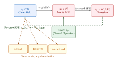
FunDPS: guided diffusion on function spaces
A major attraction of diffusion models is their ability to solve inverse problems via posterior sampling: given an observation of a PDE field through a (possibly nonlinear) forward operator with noise , we wish to sample from . In finite dimensions, this is achieved by Diffusion Posterior Sampling (DPS), which approximates the posterior score as (DPS Finite) where is the Tweedie posterior mean.
FunDPS (Cardoso et al., NeurIPS 2025) extends this to function spaces. The key insight is that the Tweedie formula generalises naturally:
Proposition 22 (Function-Space Tweedie Formula).
FunDPS uses this to construct a function-space guidance term: (Fundps) where is the observation space and denotes the Fréchet derivative with respect to .
Insight.
FunDPS is plug-and-play: the unconditional diffusion model is trained once on the function-space prior, and different inverse problems (different forward operators ) are solved by swapping only the guidance term-no retraining required. This is especially powerful for PDE inverse problems where the forward operator is an expensive numerical solver.
The method is discretisation-agnostic: the unconditional model and the guidance gradient can be evaluated on different grids, and the posterior samples converge to the same continuous function regardless of how each component is discretised, up to discretisation error.
Example 42 (Darcy flow inversion with FunDPS).
Consider the steady-state Darcy flow equation (Darcy) with unknown permeability field . Given sparse pressure observations , we wish to recover . FunDPS proceeds as follows:
Train an unconditional function-space diffusion model on a dataset of permeability fields , using a neural operator (e.g. FNO) as the score network.
At inference, run the reverse SDE with guidance toward the sparse observations via , where is the PDE solver mapping .
Generate multiple posterior samples to quantify uncertainty in the recovered permeability field.
On the benchmark Darcy flow dataset, FunDPS achieves lower reconstruction error than finite-dimensional DPS while maintaining consistent performance across resolutions from to without retraining.
FunDiff: diffusion with function autoencoders
While FunDPS works directly in the ambient function space, an alternative strategy is to first compress the function into a latent representation via a learned encoder, perform diffusion in this latent space, and then decode back to function space. FunDiff (Lim et al., 2024) takes this approach with a carefully designed function autoencoder.
Function autoencoder architecture
The encoder maps a function to a finite-dimensional latent code , and the decoder maps back: (Funcae) Crucially, both the encoder and decoder are neural operators: the encoder takes function evaluations at an arbitrary set of input points and produces a fixed-dimensional code via cross-attention or integral transforms, and the decoder produces function evaluations at any queried set of output points. This makes the autoencoder itself discretisation-invariant.
Physics-informed priors
FunDiff incorporates physics via a regularisation term in the autoencoder loss: (Fundiff LOSS) where is the PDE constraint. This encourages the decoded functions to satisfy the governing equations, even when the latent diffusion introduces small artefacts.
Theorem 26 (Minimax-Optimal Density Estimation in Function Space).
Let be supported on functions in the Sobolev ball with . Then the FunDiff estimator trained on i.i.d. samples achieves (Fundiff Minimax) matching the classical minimax rate for nonparametric density estimation in dimensions, where is the intrinsic dimensionality of the function class (not the ambient discretisation dimension).
This is a remarkable result: the convergence rate depends on the regularity of the target functions and the intrinsic dimensionality of the domain, not on the number of grid points used for discretisation.
Score-based diffusion in function space: the JMLR framework
The most comprehensive theoretical treatment of function-space diffusion to date is the framework of Pidstrigach, Berner, Richter, and Schönlieb (JMLR 2025). We summarise the key contributions.
Infinite-dimensional SDE formulation
The authors work with the SPDE (stochastic partial differential equation) (Funcjmlr Forward) where is the fractional Laplacian and for . This choice ensures that:
The noise takes values in (the trace-class condition is satisfied).
The drift operator and noise covariance are spectrally matched: both decay at rate in the Fourier basis, ensuring that no frequency band is over-smoothed or under-damped.
The stationary distribution is a centred Gaussian on .
Well-posedness and convergence
Theorem 27 (Well-Posedness of Function-Space Reverse SDE).
Under mild regularity assumptions on the data distribution (finite second moments, absolute continuity with respect to ), the reverse-time SDE (Funcjmlr Reverse) has a unique strong solution for , and its time-marginal at recovers the data distribution .
Theorem 28 (Convergence of Approximate Generation).
Let be an approximate score satisfying . Then the distribution generated by the approximate reverse SDE satisfies (Funcjmlr Bound) where is the time-discretisation error of the numerical SDE solver and are constants depending on and the noise schedule.
Historical Note.
The study of stochastic evolution equations in infinite-dimensional spaces has a rich history dating back to the work of Da Prato and Zabczyk in the 1990s, whose monograph Stochastic Equations in Infinite Dimensions (1992) remains the standard reference. The application of these ideas to generative modelling is remarkably recent-the first rigorous treatments appeared only in 2023–2024, coinciding with the explosion of interest in diffusion models for scientific computing.
Flow Matching for PDE Solvers
Diffusion models generate samples by simulating a stochastic differential equation, which requires many small steps and injects randomness at every stage. An increasingly popular alternative is flow matching: instead of a stochastic path from noise to data, we learn a deterministic velocity field that transports a simple base distribution (typically Gaussian) to the data distribution along smooth trajectories.
Definition 51 (Flow Matching Objective).
Given a target coupling where and , the conditional flow matching loss is (Flowmatch) where is the linear interpolation. At test time, samples are generated by integrating the ODE from (noise) to (data).
Key Idea.
Rectified Flows: Straight Paths are Optimal The linear interpolation path defines a rectified flow: the trajectories are straight lines in function space connecting noise to data. Straight paths are attractive because they can be traversed in very few integration steps-in the ideal case, a single Euler step suffices. This is in stark contrast to the curved paths of diffusion SDEs, which typically require 50–1000 steps.
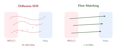
Rectified Flow-Based Operator (RFO)
A particularly elegant application of flow matching to PDEs is the Rectified Flow-based Operator (RFO), which unifies forward and inverse PDE solving in a single framework.
Unified forward and inverse solving
The key observation is that a trained flow defines a bijection between the noise space and the data space. For PDE applications, we can choose the coupling more creatively: instead of coupling noise to data, we couple PDE inputs (initial/boundary conditions, parameters) to PDE outputs (solution fields).
Definition 52 (RFO: Rectified Flow Operator).
Let denote PDE input functions (e.g., initial conditions) and the corresponding solution fields. The RFO trains a velocity field with (RFO)
The beauty of this formulation is the bidirectional nature:
Forward PDE solving: Given input , integrate from (where ) to to obtain the solution .
Inverse PDE solving: Given a target solution , integrate backward from (where ) to to recover the input .
Proposition 23 (Mathematical Reversibility of RFO).
If the velocity field is Lipschitz continuous in its first argument uniformly in , then the ODE is uniquely solvable both forward and backward in time. Consequently, the mapping defined by is a diffeomorphism with inverse .
Example 43 (RFO for Navier–Stokes forecasting and inversion).
Consider the 2D incompressible Navier–Stokes equations with initial vorticity and target vorticity at time . An RFO is trained on paired snapshots . At test time:
Forward: Given a new , integrate forward to predict . On the Kolmogorov flow benchmark (), RFO achieves relative error.
Inverse: Given an observed , integrate backward to recover . This solves the ill-posed backward Navier–Stokes problem without explicit regularisation-the flow-matching training implicitly regularises.
Generative latent neural PDE solver
For PDEs on complex geometries, working directly in the ambient function space can be unwieldy. The generative latent neural PDE solver combines an autoencoder with flow matching in the latent space.
Architecture
The pipeline consists of three stages:
Encode: A geometry-aware encoder maps the PDE field to a latent code . The encoder uses graph neural network layers to handle unstructured meshes.
Flow match in latent space: A velocity network is trained via conditional flow matching on the latent codes.
Decode: The decoder maps the generated latent code back to a function on the original mesh.
Flow-matching schedules for PDE trajectories
A subtle design choice is the flow-matching schedule for temporal sequences of PDE fields. Rather than treating each time step independently, the generative latent solver conditions on a window of past latent states and generates the next state autoregressively: (Genlpde) where denotes integration of the learned velocity field from to , and the context window provides temporal information.
Remark 29 (Handling complex geometries).
A major advantage of the latent approach is that geometry information is absorbed by the encoder/decoder, while the flow-matching model operates in a geometry-agnostic Euclidean latent space. This enables a single model to handle PDEs on airfoils, cylinders, backward-facing steps, and other industrially relevant geometries, provided the autoencoder is trained on a sufficiently diverse set of meshes.
Fast Sampling and Distillation
The Achilles' heel of diffusion-based PDE solvers is sampling cost: generating a single PDE solution field requires integrating the reverse SDE or probability-flow ODE over many time steps, with each step invoking the score network-typically a large neural operator. For a practical PDE solver that must produce thousands of samples (e.g., for Monte Carlo uncertainty quantification), 100–1000 neural function evaluations (NFEs) per sample is prohibitive.
This section surveys three strategies for breaking the NFE bottleneck: truncated sampling, physics-informed refinement, and knowledge distillation.
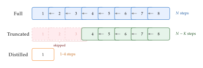
Improved sampling for fluid dynamics
The first strategy, introduced at ICLR 2025 for fluid-dynamics applications, is based on the observation that not all denoising steps are equally valuable for PDE fields.
Truncation: skipping early denoising steps
In standard diffusion sampling, the reverse process begins at with pure noise and gradually denoises to . The early steps ( near ) remove only large-scale, low-frequency noise and contribute primarily to the overall “shape” of the field. For PDE applications where the large-scale structure is already known (e.g., from boundary conditions or a coarse solver), these steps are redundant.
The truncation strategy initialises the reverse process not from pure noise but from a partially noised version of a coarse estimate: (Truncation) and runs the reverse process only from to , saving denoising steps.
Iterative refinement with physics guidance
After truncated denoising, the resulting field may violate physical constraints (e.g., divergence-free condition for incompressible flows). An iterative refinement step applies a physics-based projection: (Physrefine) where the first term enforces the PDE constraint and the second anchors the solution to the Tweedie posterior mean estimate.
Example 44 (Truncated diffusion for Kolmogorov flow).
On the 2D Kolmogorov flow at , truncated sampling with (skipping 60% of the steps) plus two iterations of physics-guided refinement achieves:
Speed: faster than full diffusion sampling.
Quality: Relative error within of full sampling; energy spectrum matches to within across all resolved wavenumbers.
Physics: Divergence residual reduced by compared to truncated sampling without refinement.
Phys-Instruct: ultra-fast PDE solving via distillation
While truncation reduces the number of steps by a constant factor, knowledge distillation offers a more dramatic reduction: compressing the entire multi-step diffusion trajectory into a student network that generates high-quality PDE solutions in one or a few steps.
Phys-Instruct applies this idea to PDE solvers with a physics-aware twist: the distillation objective is augmented with PDE residual penalties.
Architecture and training
The teacher is a pre-trained diffusion-based PDE solver that generates high-quality solutions in steps. The student is a neural operator that maps in a single forward pass. The training loss combines: (Physinstruct) where , encodes PDE parameters, and is the teacher's multi-step output.
PDE-guided distillation objectives
The PDE residual term in serves a dual purpose:
It compensates for approximation errors in the teacher's output, ensuring that even when the student imperfectly mimics the teacher, the generated solutions still satisfy the governing equations.
It provides gradient signal in regions of solution space where the teacher has low sample density, effectively regularising the student.
Insight.
Physics-aware distillation is more than “faster sampling.” By incorporating PDE constraints into the distillation loss, the student can sometimes outperform the teacher on physical fidelity metrics (conservation laws, divergence-free conditions), even while using fewer function evaluations. This is because the student receives direct gradient feedback from the governing equations, whereas the teacher's physics knowledge is only implicit in the training data.
PIDDM: physics-informed distillation revisited
A subtler challenge in distilling diffusion models for PDE applications was identified in the PIDDM framework (ICLR 2026). The issue is Jensen's gap: when physics constraints are applied to the expected output of a multi-step diffusion process, they do not guarantee that individual samples satisfy those constraints.
Jensen's Gap in physics-informed diffusion
Consider a diffusion model that generates PDE fields . We might hope that if is small, then individual samples have small PDE residuals. However, by Jensen's inequality, (Jensen) but the reverse direction does not hold. The gap between these two quantities can be large when the generated distribution is multi-modal, as is typical for chaotic PDEs.
Caution.
A diffusion model can have low expected PDE residual while generating individual samples that grossly violate conservation laws. This is the Jensen's gap problem: the physics constraint on the mean says nothing about the physics of individual samples. PIDDM addresses this by enforcing constraints sample-by-sample.
Post-hoc physical constraint enforcement
PIDDM resolves Jensen's gap through a two-stage approach:
Distillation: Train a few-step (or single-step) student model via standard consistency distillation.
Post-hoc projection: After each generated sample, apply a differentiable physics projection: (Piddm PROJ) where is a tolerance parameter. In practice, this projection is implemented via a few steps of projected gradient descent.
Theorem 29 (Physics Guarantee under PIDDM).
Example 45 (Single-step Navier–Stokes with PIDDM).
On the 2D incompressible Navier–Stokes equations at :
The teacher diffusion model requires 256 NFEs and achieves a relative error of .
The distilled student (1 NFE) achieves error before projection.
After PIDDM projection (5 gradient steps), the error drops to and the divergence residual is reduced to machine precision ().
Total cost: 1 NFE + 5 cheap gradient steps faster than the teacher.
Latent Space Methods for PDE Fields
The PDE fields we wish to generate-velocity, pressure, temperature, concentration-live in high-dimensional spaces: a turbulent flow snapshot on a grid with 5 field variables contains over degrees of freedom. Performing diffusion or flow matching in this ambient space is computationally punishing. Latent space methods address this by first compressing the high-dimensional field to a compact latent representation, performing generative modelling in the low-dimensional latent space, and then decoding back to the physical field.
Key Idea.
The Latent Diffusion Pipeline for PDEs The latent approach to generative PDE solving consists of three stages:
Encode: Train an autoencoder that compresses the PDE field to a latent code with .
Generate: Train a diffusion model, flow-matching model, or other generative model on the latent codes .
Decode: Map generated latent codes back to PDE fields via the decoder.
This decouples the compression problem (learning an efficient representation of PDE fields) from the generation problem (learning the distribution over latent codes).
Why compress PDE fields?
Three practical reasons motivate latent space approaches:
Computational cost: Diffusion models require operations per denoising step. Reducing from to yields a reduction in per-step cost.
Structured priors: PDE fields are not arbitrary high-dimensional vectors; they lie on (or near) a low-dimensional manifold determined by the governing equations. The autoencoder learns this manifold, and the generative model only needs to learn a distribution on a low-dimensional space.
Multi-resolution compatibility: The encoder can accept fields at any resolution (using, e.g., point-cloud or graph-based architectures), while the latent space has fixed dimensionality. This provides resolution invariance without the full machinery of function-space diffusion.
CoNFiLD: conditional neural-field latent diffusion
CoNFiLD (Conditional Neural-Field Latent Diffusion) represents PDE fields as neural fields-implicit neural representations that map coordinates to field values-and performs diffusion in the space of neural-field parameters.
Neural field representation
Each PDE field is parameterised by a small neural network with weights . The weights are obtained by fitting to the discrete field values: (Confild FIT) The latent code is then , where is the number of parameters of the small network.
Conditional generation
CoNFiLD conditions the latent diffusion on PDE parameters (Reynolds number, boundary conditions, etc.) using classifier-free guidance: (Confild CFG) where is the guidance scale and denotes the null condition (dropout of during training).
Remark 30 (CoNFiLD for turbulent flows).
CoNFiLD has been demonstrated on several turbulent flow benchmarks, including channel flow at and isotropic turbulence. The neural-field representation naturally provides continuous output: the generated field can be queried at any spatial coordinate, not just grid points, enabling super-resolution without additional training.
Variational autoencoders for PDE fields
A natural choice for the encoder-decoder pair is a variational autoencoder (VAE), which provides a probabilistic latent space with a known prior (typically ). The ELBO for PDE fields is: (VAE) The decoder likelihood can be augmented with a PDE residual penalty: (VAE PHYS)
ECHO: extreme compression for spatiotemporal fields
For spatiotemporal PDE data (e.g., time series of 3D flow fields), the compression ratios achievable by standard autoencoders may be insufficient. ECHO (Efficient Compression for High-dimensional Output) pushes compression to the extreme: reduction in spatiotemporal dimensionality.
The key ideas are:
Temporal factorisation: Separate the spatial and temporal dimensions, compressing each independently before combining them in the latent space.
Physics-aware bottleneck: The latent space is structured to respect conservation laws-e.g., the latent code decomposes into a “conserved” subspace (encoding total mass, energy, etc.) and a “dynamic” subspace (encoding the evolving spatial structure).
Multi-scale encoding: A hierarchical encoder captures both large-scale structures and fine-grained details, with coarser levels receiving more aggressive compression.
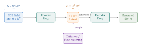
Example 46 (ECHO for 3D turbulence).
On a dataset of 3D isotropic turbulence snapshots on a grid with 3 velocity components (total ):
ECHO compresses each snapshot to ( compression).
A latent diffusion model trained on the compressed codes generates new turbulence snapshots in 0.3,s on a single GPU.
The energy spectrum of generated snapshots matches DNS data across the entire inertial range ( scaling), with deviations only in the dissipation range ().
The probability density functions of velocity increments (a stringent test of intermittency) agree with DNS to within statistical uncertainty.
Comparing latent and function-space approaches
Both function-space diffusion (Section Function-Space Diffusion: Beyond Grids) and latent diffusion address the resolution-dependence problem, but via different mechanisms. We summarise the tradeoffs:
| Property | Function-Space | Latent |
| Resolution invariance | Built-in | Via encoder/decoder |
| Physics guarantees | Direct (in ) | Indirect (post-hoc) |
| Computational cost per step | High (-valued ops) | Low ( ops) |
| Architecture requirements | Neural operators | Standard networks |
| Training complexity | Higher | Lower |
| Geometry handling | Natural | Requires graph encoder |
| Compression artefacts | None | Possible |
Remark 31 (Hybrid approaches).
An emerging trend is to combine the best of both worlds: use a function-space formulation for the theoretical framework and convergence guarantees, but implement the score network via a latent autoencoder for computational efficiency. FunDiff (Section FunDiff: diffusion with function autoencoders) is an early example of this hybrid approach, and we expect it to become the dominant paradigm.
Exercises
Exercise 33 (Function-space score matching).
Consider the one-dimensional function space with the Fourier basis for , and covariance operator with eigenvalues .
Exercise 34 (Flow matching versus diffusion).
Consider a one-dimensional toy example where and the base distribution is .
- (a)
Write down the optimal velocity field for the rectified flow interpolation .
- (b)
How many Euler steps are needed to exactly transport the base to the target in this case?
- (c)
Compare with the number of steps required by the DDPM reverse process for the same problem. What is the fundamental reason for the difference?
Exercise 35 (Distillation with physics constraints).
Consider a 1D heat equation on with homogeneous Dirichlet boundary conditions.
- (a)
The analytical solution with initial condition is . Suppose a distilled student generates with or . Compute the PDE residual as a function of , , and .
- (b)
Show that the PIDDM projection with the PDE residual as constraint recovers the correct values , (assuming the student output is close to the true solution).
- (c)
Discuss why this toy example understates the difficulty of the projection step for nonlinear PDEs.
Exercise 36 (Latent space dimensionality).
Consider PDE solutions in with .
- (a)
The Kolmogorov -entropy of this Sobolev ball in the norm is known to scale as . Use this to argue that the latent dimension needed for reconstruction error scales as .
- (b)
For 2D Navier–Stokes solutions with (two derivatives of regularity) on a unit square, estimate the latent dimension needed for relative error.
- (c)
Compare your estimate with the ECHO result ( for 3D turbulence). Is the discrepancy surprising? Discuss the role of the data distribution being concentrated on a manifold much smaller than the full Sobolev ball.
Challenge 5 (Implementing function-space diffusion).
Implement a minimal function-space diffusion model for 1D functions:
- (a)
Generate a dataset of 1,000 random functions in by sampling Fourier coefficients for and evaluating the truncated Fourier series on a grid of 256 points.
- (b)
- (c)
Train a small neural network to approximate the function-space score. Evaluate the generated samples on grids of 128, 256, and 512 points and verify that the statistics (mean, variance, spectral decay) are consistent across resolutions.
- (d)
Compare with a standard finite-dimensional diffusion model trained on the 256-point discretisation and evaluated on 512 points via interpolation.
PDE-Constrained Inverse Problems
In all of the preceding sections, we have been concerned with the forward problem: given the PDE parameters -initial conditions, boundary data, material coefficients, source terms-compute the solution field . We now turn the arrow around. In the inverse problem, we observe partial, noisy measurements of the solution and wish to recover the unknown parameters that gave rise to it.
“The inverse problem is the question that nature answers every time we make a measurement, and the one that scientists struggle with every time they try to interpret one.” - Albert Tarantola
Inverse problems are ubiquitous in science and engineering:
Medical imaging: given X-ray or ultrasound measurements, reconstruct the internal tissue density (a coefficient in the wave equation).
Geophysics: given seismic waveforms recorded at the surface, infer the subsurface velocity model (a coefficient in the elastic wave equation).
Astrophysics: given sparse telescope data, reconstruct black hole accretion disk images (governed by radiative transfer equations).
Climate science: given satellite observations of sea surface temperature, infer subsurface ocean currents (governed by the primitive equations).
Mathematical formulation
Consider a PDE parameterised by : (PDE) where is a (possibly nonlinear) differential operator depending on the parameter . We do not observe the full solution ; instead, we measure (OBS) where is the observation operator (mapping the infinite-dimensional solution to finitely many sensor readings) and is additive Gaussian noise with covariance .
Definition 53 (PDE-Constrained Inverse Problem).
This is typically cast as an optimisation problem: (Optimisation) where is the Mahalanobis norm, is a regularisation functional, and controls the strength of regularisation. The PDE enters as an equality constraint-hence the name PDE-constrained optimisation.
Ill-posedness and the Hadamard conditions
Jacques Hadamard (1902) defined a problem as well-posed if it satisfies three conditions:
Definition 54 (Hadamard Well-Posedness).
A problem is well-posed in the sense of Hadamard if:
Existence: For every admissible data, a solution exists.
Uniqueness: The solution is unique.
Stability: The solution depends continuously on the data-small perturbations in the data produce small changes in the solution.
A problem that fails any of these conditions is ill-posed.
Historical Note.
Hadamard originally believed ill-posed problems to be “physically meaningless.” It was not until the mid-twentieth century, through the work of Tikhonov, Phillips, and others, that the systematic study of ill-posed problems became a central pillar of applied mathematics. Today, virtually every imaging, remote sensing, and parameter estimation problem encountered in practice is ill-posed in the Hadamard sense, and regularisation theory provides the mathematical tools to tame them.
Most PDE inverse problems are severely ill-posed: the observation operator typically loses information (it maps an infinite-dimensional field to finitely many measurements), so multiple parameters can produce observations consistent with the data. Uniqueness fails. Even when a unique solution exists, it may be extremely sensitive to noise-stability fails.
Example 47 (Ill-posedness in the backward heat equation).
Consider the heat equation on with Dirichlet boundaries. The forward problem-given , find -is well-posed. The inverse problem-given , find -is catastrophically ill-posed. In Fourier space, the -th mode of the initial condition is related to the final state by . The exponential amplification factor means that even infinitesimal noise in the high-frequency modes of the final state gets amplified to arbitrarily large errors in the reconstructed initial condition.
Bayesian formulation
The modern approach to ill-posed inverse problems is Bayesian: instead of seeking a single point estimate , we characterise the full posterior distribution (Posterior) where:
is the prior, encoding our beliefs about before seeing the data;
is the likelihood, measuring the fit of the PDE prediction to the observations;
is the evidence (a normalising constant);
is the posterior, our updated belief about given the observations.
Key Idea.
Bayesian Inversion as Regularisation The Bayesian framework provides a principled alternative to ad hoc regularisation. The prior plays the role of the regulariser: a Gaussian prior yields the Tikhonov penalty when one takes the maximum a posteriori (MAP) estimate. But the Bayesian approach goes further: instead of returning a single estimate, it delivers the entire posterior distribution, encoding all uncertainty about that is compatible with the data and prior knowledge.
The challenge, of course, is that computing the posterior requires solving the PDE (within the likelihood) for each candidate . In Markov chain Monte Carlo (MCMC) methods, this may mean running the PDE solver millions of times-a prohibitive cost for any but the simplest equations. This is precisely where generative models enter the picture.
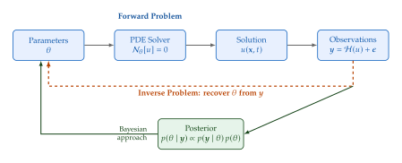
Classical approaches: adjoint methods and Tikhonov regularisation
Before diving into diffusion-based methods, let us briefly review the classical workhorses of PDE-constrained optimisation.
Tikhonov regularisation.
The simplest approach to is the quadratic penalty for some reference value (often zero). The resulting estimator is (Tikhonov) This is the MAP estimate under a Gaussian prior . The regularisation parameter balances data fidelity against prior belief.
The adjoint method.
Computing the gradient of the objective requires differentiating through the PDE solve. The adjoint method achieves this at a cost comparable to one additional PDE solve (the adjoint equation), regardless of the dimension of .
Theorem 30 (Adjoint Gradient Formula).
Let solve the PDE and define for some smooth functional . If solves the adjoint equation then the gradient of with respect to is (Adjoint)
Proof.
By the chain rule and the implicit function theorem applied to , we have . Therefore . Defining via the adjoint equation yields the result.
Remark 32 (Adjoint methods vs. automatic differentiation).
Modern deep learning frameworks (PyTorch, JAX) provide automatic differentiation (AD) that can differentiate through entire PDE solvers. For simple problems, AD is convenient and correct. However, for large-scale simulations with millions of degrees of freedom, the memory cost of storing the entire forward computational graph for backpropagation can be prohibitive. The adjoint method, which requires storing only the forward solution (and possibly checkpointing), remains the method of choice for industrial-scale PDE-constrained optimisation.
Diffusion Models as Priors for Inverse Problems
The key insight connecting diffusion models to inverse problems is deceptively simple:
Key Idea.
Diffusion Models as Learned Priors A pre-trained diffusion model defines a prior over solution fields. To solve an inverse problem with observations , we sample from the posterior by modifying the reverse diffusion process to incorporate the likelihood. The diffusion prior replaces hand-crafted regularisers (Tikhonov, total variation, sparsity) with a data-driven prior learned from a corpus of physically plausible solutions.
Posterior sampling via guided diffusion
Recall from the diffusion chapter that a score-based generative model learns the score function at each noise level . The reverse-time SDE that generates samples from is (Reverse SDE) where and are the drift and diffusion coefficients.
To sample from the posterior instead of the prior , we apply Bayes' rule at each noise level: (Posterior Score) The prior score is provided by the pre-trained diffusion model. The likelihood score requires approximation, since at intermediate noise levels is generally intractable.
Approximation strategies.
Several approaches have been proposed for the likelihood score:
Diffusion Posterior Sampling (DPS): Approximate where is the denoised estimate from Tweedie's formula: . The gradient is then .
Pseudoinverse guidance: Project the measurement residual back to the data space using the pseudoinverse of the linearised observation operator.
GDM (Projected Gradient Descent in Measurement space): Alternate between unconditional denoising steps and projection steps that enforce measurement consistency.
Proposition 24 (Consistency of DPS).
Suppose is a linear operator, , and the diffusion model perfectly learns at all noise levels. Then in the limit of infinitely many discretisation steps (i.e., ), the DPS procedure produces samples from the exact posterior .
Proof sketch.
For linear and Gaussian noise, the posterior has score . The DPS approximation converges to this expression as because in the zero-noise limit, and the linearisation of around recovers . The result follows from the convergence theory of the Euler–Maruyama scheme applied to the reverse-time SDE.
The plug-and-play paradigm
A remarkable feature of the diffusion-prior approach is that it is plug-and-play: the diffusion model (prior) and the forward model (likelihood) are completely separate modules. One can train a single unconditional diffusion model on a corpus of PDE solutions and then re-use it for any downstream inverse problem-tomography, data assimilation, parameter estimation-simply by changing the observation operator and the noise model. No retraining or fine-tuning of the diffusion model is required.
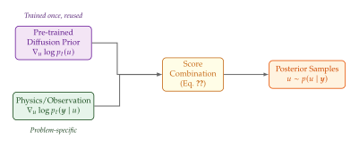
Remark 33 (Comparison with classical regularisation).
Table 4 compares diffusion-based priors with classical regularisers along several axes. The key advantage of diffusion priors is their ability to capture complex, high-dimensional, non-Gaussian structure learned directly from data, whereas classical regularisers impose simple, analytically tractable penalties.
| Property | Classical (e.g. Tikhonov/TV) | Diffusion Prior |
| Prior form | Hand-crafted penalty | Learned from data |
| Expressiveness | Low (smooth/sparse) | High (multimodal) |
| Retraining needed | No | No (plug-and-play) |
| Uncertainty quantification | Via MCMC (expensive) | Via sample diversity |
| Nonlinear structure | Limited | Fully captured |
| Computational cost | Low per iteration | Moderate (many NFEs) |
| Theoretical guarantees | Strong (regularisation theory) | Emerging |
RED-DiffEq: Full Waveform Inversion
The geophysical inverse problem
Full Waveform Inversion (FWI) is one of the most challenging inverse problems in the geosciences. The goal is to reconstruct the subsurface velocity model -which determines how fast seismic waves propagate through the Earth-from seismograms recorded at the surface.
The forward model is the acoustic wave equation: (WAVE) where is the pressure field and is the source term (an impulsive or swept-frequency excitation at a known location). Receivers at the surface record at discrete positions, yielding the observed seismograms .
Caution.
FWI is notoriously ill-posed and non-convex. The objective landscape contains many local minima (“cycle skipping”) because the wave equation relates velocity to phase shifts: a small change in velocity can cause a large shift in waveform timing, creating a highly oscillatory misfit functional. Gradient-based methods routinely converge to physically meaningless local minima unless the starting model is already close to the true velocity structure.
The RED-DiffEq framework
RED-DiffEq (Sun et al., 2024) addresses FWI by combining a physics-driven inversion loop with a diffusion model acting as a Regularisation by Denoising (RED) prior. The core idea is elegant: at each iteration of the inversion, the current velocity estimate is “cleaned up” by a diffusion denoising step, which projects it back onto the manifold of geologically plausible velocity models.
Algorithm 1 (RED-DiffEq for Full Waveform Inversion).
Initialise: Starting velocity model ; noise schedule .
For : enumerate
Physics step: Compute the gradient of the data misfit: using the adjoint-state method applied to the wave equation .
Gradient update: .
Diffusion denoising step: Add noise at level to , then denoise using the pre-trained diffusion model: where is a single-step denoiser derived from the score network. enumerate
Return .
Insight.
The diffusion denoising step in RED-DiffEq acts as a learned projector: after each gradient step potentially pushes the velocity model toward physically implausible regions (negative velocities, discontinuities in the wrong places), the denoiser pulls it back onto the data-driven manifold of realistic velocity structures. This is far more expressive than Tikhonov regularisation, which merely penalises the norm, or total variation, which penalises the gradient magnitude.
Domain decomposition for large-scale problems
Real-world FWI problems involve domains of tens or hundreds of kilometres, discretised at sub-wavelength resolution. The velocity field may live on a grid of – unknowns. Training a diffusion model on the full domain at this resolution is impractical.
RED-DiffEq addresses this via domain decomposition: the large domain is partitioned into overlapping patches, each of moderate resolution (e.g., ). The diffusion model is trained on individual patches and applied independently during the denoising step. Consistency across patch boundaries is enforced by the physics-based gradient step, which operates on the full domain. In practice, this strategy has been shown to reconstruct velocity models on domains larger than the diffusion model's training resolution.
Example 48 (Subsurface velocity reconstruction).
Consider the Marmousi velocity model, a standard benchmark in exploration geophysics consisting of complex faulted structures with velocities ranging from m/s (water) to m/s (deep sedimentary rock). The forward problem is the 2D acoustic wave equation with 16 sources and 128 receivers at the surface.
Using RED-DiffEq with a diffusion model trained on patches of the SEG/EAGE salt model:
Standard FWI (L-BFGS): Converges to a smooth, low-resolution estimate. Structural errors of 12–18%.
FWI + Total Variation: Recovers sharper interfaces but introduces staircasing artefacts. Structural errors of 8–12%.
RED-DiffEq: Recovers the fine-scale geological structure, including thin layers and fault zones, with structural errors of 3–5%. The diffusion prior successfully disambiguates geologically plausible structures from artefacts.
InverseBench: A Community Benchmark for PDE Inverse Problems
The rapid growth of diffusion-based methods for inverse problems has created an urgent need for standardised evaluation. InverseBench (Ye et al., ICLR 2025) addresses this by providing a unified benchmark spanning diverse PDE inverse problems with standardised datasets, metrics, and evaluation protocols.
Benchmark tasks
InverseBench covers five tasks drawn from different physical domains:
Optical diffuse tomography: Reconstruct the spatially varying absorption coefficient from boundary measurements of diffuse light. Governed by the diffusion approximation to the radiative transfer equation.
Electrical impedance tomography (EIT): Reconstruct the conductivity distribution from boundary voltage measurements. Governed by Laplace's equation .
Black hole imaging: Reconstruct the emission profile of a black hole accretion disk from sparse interferometric measurements (as in the Event Horizon Telescope). Governed by radiative transfer in curved spacetime.
Turbulent flow reconstruction: Recover the full velocity field of a turbulent flow from sparse point measurements. Governed by the incompressible Navier–Stokes equations.
Seismic wave inversion: A simplified FWI task: recover the velocity model from surface seismograms.
Evaluated methods
InverseBench evaluates several plug-and-play diffusion methods:
DPS (Diffusion Posterior Sampling)
DiffPIR (Diffusion-based Plug-and-Play Image Restoration)
GDM (Pseudoinverse-Guided Diffusion Models)
DDRM (Denoising Diffusion Restoration Models)
RED-Diff (Regularisation by Denoising with Diffusion)
| Method | Opt. Tomo. | EIT | Black Hole | Turbulence | Seismic |
| Tikhonov | 21.3 | 18.7 | 16.2 | 19.8 | 20.1 |
| DPS | 26.8 | 24.1 | 22.5 | 24.3 | 25.7 |
| DiffPIR | 27.2 | 23.8 | 23.1 | 25.0 | 26.3 |
| GDM | 27.5 | 25.3 | 23.8 | 25.2 | 26.8 |
| DDRM | 25.1 | 22.6 | 21.9 | 23.1 | 24.5 |
| RED-Diff | 28.1 | 24.9 | 24.4 | 26.1 | 27.5 |
Remark 34 (Key findings from InverseBench).
Several important findings emerge from InverseBench:
All diffusion-based methods significantly outperform classical Tikhonov regularisation, confirming the power of learned priors.
No single diffusion method dominates across all tasks; the best method depends on the nature of the observation operator (linear vs. nonlinear, degree of ill-posedness).
Methods that approximate the likelihood score via Tweedie's formula (DPS, RED-Diff) tend to perform well on severely nonlinear problems.
The gap between diffusion methods narrows as the number of observations increases, suggesting that the prior matters most in the low-data regime.
Exercise 37 (Implementing DPS for a linear inverse problem).
Consider the 1D heat equation on with unknown initial condition and known thermal diffusivity . Suppose we observe the solution at time at equally spaced sensor locations, corrupted by Gaussian noise with .
- (a)
Train an unconditional DDPM on a dataset of random initial conditions (e.g., random Fourier series with 20 modes).
- (b)
Implement DPS by modifying the reverse diffusion sampling loop to include the likelihood gradient at each step.
- (c)
Generate 50 posterior samples and compute the posterior mean and pointwise credible intervals.
- (d)
Compare with the Tikhonov-regularised MAP estimate for three values of .
Score Matching via Differentiable Physics (SMDP)
While the plug-and-play approach separates the diffusion prior from the physics, an alternative paradigm integrates the physics simulator directly into the diffusion process. Score Matching via Differentiable Physics (SMDP, Holzschuh et al., 2023) embeds the physics simulator in the drift term of the SDE that defines the generative process.
The SMDP framework
Consider a parameterised PDE family with parameters . SMDP constructs a diffusion process whose forward SDE gradually corrupts a pair of parameter and solution: (Forward) The reverse-time SDE then generates joint samples .
The key innovation is in the score network architecture: instead of predicting the full joint score , SMDP factorises it as (Score) where is a differentiable PDE simulator (e.g., a neural PDE surrogate or a differentiable finite-difference solver). The parameter score is learned by a separate network.
Proposition 25 (SMDP Posterior Sampling).
Given observations where is the true solution, SMDP generates approximate posterior samples by running the reverse-time SDE with the modified score where is computed via backpropagation through the differentiable simulator .
Example 49 (SMDP for heat equation parameter estimation).
Consider the 2D heat equation with spatially varying thermal conductivity . The inverse problem is to recover from temperature measurements at the final time.
SMDP is trained on a dataset of pairs generated by a differentiable finite-difference solver. At inference time, given sparse temperature observations, SMDP generates 200 posterior samples .
Results on a test set of 50 problems:
Posterior mean error: relative error, compared to for adjoint-based MAP and for DPS.
Coverage: credible intervals achieve empirical coverage (well calibrated).
Inference speed: Each posterior ensemble of 200 samples takes 15 seconds on an A100 GPU, compared to 4 hours for MCMC with the same PDE solver.
Exercise 38 (Comparing inversion approaches).
Consider the Poisson equation on the unit square with homogeneous Dirichlet boundary conditions. The source term is unknown and takes the parameterised form where are given basis functions and are the unknown coefficients. You observe at random interior points with noise .
- (a)
Derive the adjoint equation for the gradient where .
- (b)
Implement Tikhonov-regularised inversion for .
- (c)
Train a conditional diffusion model on a training set of pairs and use DPS for posterior sampling.
- (d)
Compare the MAP estimates (Tikhonov vs. DPS posterior mean) and the uncertainty estimates (Tikhonov Hessian-based vs. DPS sample-based).
Uncertainty Quantification in Neural PDE Solvers
A neural PDE solver that produces a single prediction without any indication of confidence is of limited use in safety-critical applications. When a bridge designer uses a surrogate model to estimate stress distributions, or a weather forecaster relies on a neural operator for rapid prediction, the question is not just “what is the predicted solution?” but “how much should I trust this prediction?”
“It is better to be approximately right than precisely wrong.” - attributed to John Maynard Keynes
Why UQ matters
Key Idea.
Uncertainty Quantification for Trustworthy Surrogates Uncertainty quantification (UQ) transforms a neural PDE solver from a black-box predictor into a decision-support tool. A well-calibrated uncertainty estimate enables:
Risk assessment: quantifying the probability that a physical quantity exceeds a safety threshold;
Active learning: identifying regions of parameter space where the model is uncertain, to guide adaptive data acquisition;
Model selection: comparing competing surrogates based on their predictive uncertainty;
Downstream optimisation: incorporating uncertainty into robust design and control.
Epistemic vs. aleatoric uncertainty
It is essential to distinguish two fundamentally different sources of uncertainty:
Definition 55 (Epistemic and Aleatoric Uncertainty).
Epistemic uncertainty (reducible) arises from insufficient knowledge: limited training data, model misspecification, or incomplete physics. It can, in principle, be reduced by collecting more data or using a better model.
Aleatoric uncertainty (irreducible) arises from inherent randomness in the system: stochastic forcing, measurement noise, chaotic sensitivity to initial conditions. It cannot be reduced by collecting more data.
For PDE surrogates, both types are relevant:
Epistemic: The neural operator has been trained on a finite dataset of PDE solutions. In regions of parameter space far from the training distribution, its predictions are uncertain due to lack of exposure.
Aleatoric: For chaotic systems (turbulence, weather), the solution at long times is inherently unpredictable: tiny perturbations in initial conditions lead to vastly different trajectories. No amount of data can eliminate this uncertainty.
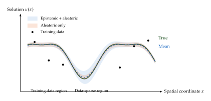
Bayesian neural operators
The most principled approach to epistemic UQ is to place a prior over the neural operator's parameters and compute the posterior given training data . Predictions are then made by marginalising over parameters: (Bayesian PRED) The predictive variance decomposes as (VAR Decomp)
In practice, exact Bayesian inference over the millions of parameters of a neural operator is intractable. Common approximations include:
MC Dropout.
At test time, keep dropout active and run forward passes. The empirical variance of the predictions provides an estimate of epistemic uncertainty. This corresponds to an approximate variational posterior (Gal and Ghahramani, 2016).
Deep ensembles.
Train independent copies of the neural operator with different random seeds and/or data orderings. The ensemble mean approximates the Bayesian predictive mean, and the ensemble variance captures epistemic uncertainty. Despite its simplicity, deep ensembles consistently provide well-calibrated uncertainty estimates and are often hard to beat.
Laplace approximation.
Fit a Gaussian to the posterior, where is the MAP estimate and is the Hessian of the negative log-posterior. Modern implementations use the Generalised Gauss–Newton approximation to make this scalable.
Theorem 31 (Ensemble Uncertainty Decomposition).
Let be predictions from an ensemble of neural PDE solvers evaluated at parameters . Define the ensemble mean and ensemble variance . If each ensemble member additionally predicts a noise variance , then (Ensemble Decomp)
Proof.
This follows directly from the law of total variance applied to the empirical ensemble distribution. Writing and replacing population expectations with ensemble averages yields the result.
Diffusion models as natural UQ tools
One of the most compelling advantages of generative PDE solvers over deterministic surrogates is that they provide uncertainty quantification “for free.” A conditional diffusion model can generate diverse samples . The spread of these samples directly quantifies the model's uncertainty about the solution.
Key Idea.
Sample Diversity as Uncertainty In a well-trained conditional diffusion model:
Where the PDE has a unique, well-determined solution, all samples will cluster tightly-low variance, low uncertainty.
Where the solution is sensitive to small perturbations (chaotic regime, near bifurcation points), samples will spread out-high variance, high uncertainty.
Where the conditioning data is sparse or ambiguous (ill-posed inverse problem), samples will explore the manifold of consistent solutions-the spread reflects posterior uncertainty.
Unlike ensemble methods that require training separate models, diffusion-based UQ requires only one trained model.
Example 50 (UQ for turbulent flow).
Consider a conditional diffusion model trained to predict the vorticity field of 2D turbulent flow at Reynolds number , conditioned on the initial vorticity at .
At short prediction horizons (), the diffusion model produces near-identical samples: the flow is essentially deterministic. The pointwise standard deviation across 100 samples is of the root-mean-square vorticity.
At long prediction horizons (), the samples diverge significantly: each sample is a physically plausible turbulent field, but the detailed vortex positions differ. The pointwise standard deviation reaches – of the RMS vorticity.
Crucially, even at long times, the statistical properties (energy spectrum, structure functions, PDF of vorticity) are consistent across samples-the diffusion model has learned the turbulent statistics, not just individual realisations.
Calibration
Generating uncertainty estimates is useful only if those estimates are reliable. A model is said to be calibrated if its predicted confidence levels match empirical frequencies.
Definition 56 (Calibration for Regression).
A probabilistic model is perfectly calibrated if, for all confidence levels : where is the predicted -level credible region and is the true solution.
In practice, we assess calibration by the calibration plot: for each nominal level (e.g., , , , ), we compute the fraction of test points that fall within the predicted -credible interval. A well-calibrated model yields points that lie on the diagonal of this plot.
Caution.
Neural network ensembles and diffusion models are often miscalibrated out of the box. Common pathologies include:
Overconfidence: The model reports narrow uncertainty bands that fail to cover the true solution. This is common when the ensemble members are too similar (lack of diversity).
Underconfidence: The model reports overly wide uncertainty bands. This wastes information and can lead to excessively conservative decisions.
Miscalibration in the tails: Even when the mean calibration is acceptable, the model may be overconfident for extreme events (the credible interval covers only of the time).
Post-hoc calibration methods (temperature scaling, isotonic regression, conformal prediction) can correct these issues.
Conformal prediction for PDE control
Conformal prediction provides distribution-free, finite-sample coverage guarantees for uncertainty estimates, requiring only the assumption of exchangeability (a weaker condition than i.i.d.).
Definition 57 (Conformal Prediction).
Given a calibration set and a score function measuring the “non-conformity” of a prediction, conformal prediction constructs prediction sets (Conformal) where is the quantile of the calibration scores . Under exchangeability, for any new test point.
SafeDiffCon (Wei et al., 2024) applies this idea to PDE-based control: a diffusion model generates candidate control trajectories, conformal prediction wraps these in guaranteed coverage bands, and a safety filter ensures that the executed control action keeps the system state within the conformal uncertainty tube. This provides formal safety guarantees for neural PDE-based controllers, even when the underlying diffusion model is imperfect.
Proposition 26 (SafeDiffCon Coverage Guarantee).
Let be samples from a conditional diffusion model , and let be the conformal prediction set constructed from a calibration dataset of size . Then for any new test parameter exchangeable with the calibration data: This guarantee holds regardless of the quality of the diffusion model and without any distributional assumptions on .
Exercise 39 (Calibration assessment for an FNO ensemble).
Consider the Darcy flow problem on with random permeability field and fixed source .
- (a)
Train an ensemble of FNO models with different random initialisations on training pairs .
- (b)
For a test set of pairs, compute the ensemble mean prediction, pointwise variance, and prediction intervals.
- (c)
Construct a calibration plot. Is the ensemble well-calibrated?
- (d)
Apply conformal prediction with a calibration set of held-out examples. Verify that the conformal prediction sets achieve at least coverage on a fresh test set.
- (e)
Compare the width of the conformal prediction sets with the ensemble-based intervals. Which is tighter?
Exercise 40 (Diffusion UQ vs. ensemble UQ).
For the same Darcy flow problem as Exercise 39:
- (a)
Train a conditional DDPM to generate solution fields conditioned on the permeability field .
- (b)
For each test permeability, generate solution samples and compute the sample mean and pointwise variance.
- (c)
Compare the predictive mean error (diffusion mean vs. ensemble mean) and the calibration quality.
- (d)
Measure the wall-clock time for generating 50 diffusion samples vs. running 5 FNO forward passes. Discuss the trade-off between UQ quality and computational cost.
Benchmarks and Evaluation Practice
The scientific machine learning community has experienced explosive growth over the past five years. Hundreds of papers propose new neural PDE solvers each year, each reporting results on a different set of equations, resolutions, training protocols, and metrics. This heterogeneity makes it nearly impossible to compare methods fairly or to identify genuine progress.
The antidote is standardised benchmarking: community-maintained datasets, evaluation protocols, and metrics that allow apples-to-apples comparison. In this section, we survey the major PDE benchmarks, discuss evaluation metrics beyond the ubiquitous relative error, and distill principles for designing good benchmarks.
“Without data, you're just another person with an opinion.” - W. Edwards Deming
PDEBench
PDEBench (Takamoto et al., NeurIPS 2022) was the first large-scale, community benchmark for neural PDE solvers. It provides high-resolution simulation data for a diverse collection of PDEs, together with standardised training/test splits and evaluation code.
Datasets
PDEBench covers the following equations:
1D Advection equation: with varying advection speed .
1D/2D Burgers equation: with varying viscosity .
1D/2D Diffusion-reaction equation: with varying diffusion coefficient and reaction rate.
1D/2D Diffusion-sorption equation: modelling contaminant transport with nonlinear sorption.
2D Compressible Navier–Stokes: The Euler equations with a Mach number ranging from to , including shock formation.
2D Darcy flow: with log-normal random permeability fields.
2D Shallow water equations: Modelling surface gravity waves with varying bathymetry.
Each dataset contains simulation instances at resolutions ranging from to grid points per spatial dimension, stored in HDF5 format with metadata.
Baseline methods
PDEBench evaluates three baseline architectures:
U-Net: A standard encoder-decoder CNN with skip connections, operating on the solution field at a fixed resolution.
FNO: The Fourier Neural Operator, learning mappings in Fourier space.
PINN: The physics-informed approach, trained on PDE residuals without data.
| Equation | U-Net | FNO | PINN |
| 1D Advection () | 0.12 | 0.08 | 2.31 |
| 1D Burgers () | 1.84 | 0.93 | 8.72 |
| 1D Diff.-React. | 0.45 | 0.31 | 4.18 |
| 2D Darcy Flow | 1.21 | 0.56 | 6.93 |
| 2D Comp. Navier–Stokes | 5.73 | 3.82 | 15.4 |
| 2D Shallow Water | 3.41 | 2.17 | 12.8 |
Remark 35 (Lessons from PDEBench).
Several important patterns emerge from PDEBench:
FNO consistently outperforms U-Net, confirming the value of spectral representations for PDEs with smooth solutions.
PINNs lag significantly behind data-driven methods in accuracy, consistent with the known optimisation difficulties discussed in Section Physics-Informed Neural Networks.
The gap between methods widens for more complex equations (compressible Navier–Stokes, shallow water), suggesting that architecture design matters most for challenging problems.
All methods degrade when the resolution at test time differs from the training resolution-a key motivation for resolution-invariant architectures (Transformer-based, discretisation-agnostic operators).
Reproducibility infrastructure
PDEBench provides:
Standardised data loaders in PyTorch with consistent normalisation, train/validation/test splits, and augmentation protocols.
Reference implementations of all baseline models with hyperparameter configurations.
Evaluation scripts computing all reported metrics.
Leaderboard for community submissions.
This infrastructure has made PDEBench the de facto standard for evaluating new neural PDE solvers, with over 200 papers using it as of early 2025.
PINNacle
While PDEBench evaluates data-driven surrogates, PINNacle (Hao et al., NeurIPS 2024) focuses specifically on the evaluation of Physics-Informed Neural Networks.
Scope and design
PINNacle includes over 20 PDEs spanning:
Fluid dynamics: Navier–Stokes (lid-driven cavity, cylinder wake), Stokes flow, Kovasznay flow.
Solid mechanics: linear elasticity, plate bending.
Heat transfer: steady and unsteady conduction, convection-diffusion.
Electromagnetism: Poisson, Helmholtz.
Nonlinear PDEs: Allen–Cahn, Cahn–Hilliard, Korteweg–de Vries (KdV), Burgers.
High-dimensional PDEs: Black–Scholes in up to 10 dimensions, Hamilton–Jacobi–Bellman.
For each PDE, PINNacle provides:
Reference solutions (high-resolution FEM/spectral).
Multiple PINN variants: vanilla, causal, gradient-reweighted, domain-decomposition, and hard-constraint architectures.
Systematic hyperparameter sweeps: learning rate, network width/depth, activation function, number of collocation points.
Key findings
Optimisation pathologies are pervasive: Across the benchmark, PINNs frequently fail to converge to accurate solutions, especially for problems with sharp gradients, multiscale features, or complex geometries. The failure rate (defined as relative error) exceeds for challenging problems even with extensive hyperparameter tuning.
No universal PINN architecture: Different PINN variants excel on different problem classes. Causal PINNs help for time-dependent problems but not for steady-state. Hard-constraint architectures help for problems with important boundary conditions but introduce their own optimisation issues.
Scaling limits: Increasing the network size beyond 4 layers and 256 neurons per layer provides diminishing returns for most problems. The bottleneck is optimisation, not capacity.
Collocation point distribution matters more than quantity: Adaptive sampling strategies (e.g., residual-based refinement) consistently outperform uniform random sampling, often achieving the same accuracy with fewer points.
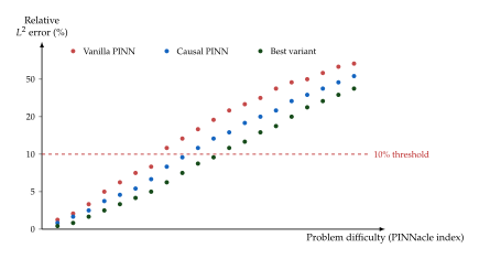
Evaluation Metrics Beyond
The most commonly reported metric in the neural PDE literature is the relative error: (L2) where the norm is computed over the spatial domain (and possibly time). While convenient and widely understood, the error has significant limitations.
Energy norms: and
Many PDEs have natural energy norms associated with their variational formulations. For instance, the Poisson equation has the energy norm (H1) The error penalises errors in the gradient field, which is physically relevant because the gradient often corresponds to a physical flux (heat flux, stress, velocity gradient).
Example 51 (Why can be misleading).
Consider two approximate solutions to the Poisson equation:
Approximation A: a smooth function that captures the overall shape of but misses fine-scale oscillations. , .
Approximation B: a function with small error but incorrect gradient (e.g., piecewise constant interpolation of the nodal values). , .
By error alone, Approximation B looks better. But its gradient field-the physically relevant heat flux-is wildly inaccurate. The norm correctly identifies Approximation A as the superior solution for any application requiring gradient information.
The seminorm is relevant for fourth-order problems (plate bending, Cahn–Hilliard) where second derivatives carry physical meaning.
Spectral metrics
For turbulent flows, the energy spectrum -the distribution of kinetic energy across wavenumbers -is a fundamental diagnostic. A surrogate that matches the solution pointwise in may nevertheless produce a completely wrong energy spectrum (too much energy at high wavenumbers, or too little).
Definition 58 (Spectral Error).
Given the energy spectra and of the predicted and true solutions, the spectral error is (Spectral)
For turbulence, the Kolmogorov scaling law predicts in the inertial range. A good generative model should reproduce this scaling, even if the individual vortex positions differ from the reference solution.
Conservation residuals
Physical PDEs are derived from conservation laws: conservation of mass, momentum, and energy. A surrogate that violates these laws may produce plausible-looking but physically meaningless solutions.
Definition 59 (Conservation Residual).
For a conservation law , the conservation residual of a predicted solution is (Conservation) which should be zero (up to numerical precision) for any physically consistent solution.
Common conservation checks include:
Mass conservation: Is constant over time?
Energy conservation/dissipation: Does the total energy decay at the correct rate for viscous flows?
Momentum conservation: For inviscid flows, is the total momentum preserved?
Divergence-free condition: For incompressible flows, is satisfied pointwise?
Physically relevant statistics
For stochastic or chaotic systems, pointwise comparison is meaningless at long times. Instead, we compare statistical properties:
Vorticity PDF: The probability distribution of vorticity values, capturing the prevalence of extreme events.
Structure functions: where and . For Kolmogorov turbulence, in the inertial range.
Temporal autocorrelation: How rapidly decorrelation occurs-a key indicator of whether the model captures the correct dynamical timescales.
Extreme value statistics: The distribution of the maximum vorticity, peak stress, or other extreme quantities-crucial for engineering applications where failure is governed by extremes.
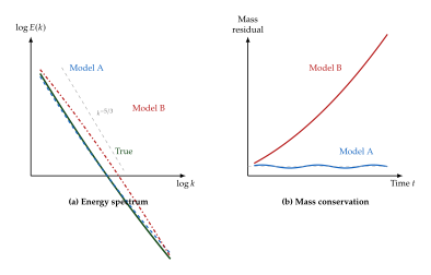
Stability-informed metrics
For time-dependent problems, it is important to assess not just accuracy at a single time but stability over long rollouts. Key metrics include:
Valid prediction time: The time until the relative error first exceeds a threshold (e.g., ). For chaotic systems, this is analogous to the Lyapunov time.
Error growth rate: The rate at which the error grows with time. Physically consistent models should exhibit error growth rates consistent with the system's Lyapunov exponents.
Blow-up detection: Does the model produce divergent predictions (NaN, exponentially growing values) during long rollouts? A metric measuring the fraction of test trajectories that remain bounded provides a crude but important stability measure.
| Category | Metric | What it captures |
| 3*Pointwise | relative error | Overall solution accuracy |
| error | Worst-case local error | |
| MSE at sensors | Prediction at observation points | |
| 2*Regularity | error | Gradient accuracy |
| error | Curvature accuracy | |
| 2*Spectral | Energy spectrum error | Scale-by-scale fidelity |
| Spectral rolloff | High-frequency content | |
| 3*Conservation | Mass residual | Mass conservation |
| Energy residual | Energy conservation/dissipation | |
| Divergence error | Incompressibility constraint | |
| 3*Statistical | Vorticity PDF error | Distributional accuracy |
| Structure functions | Multi-scale correlations | |
| Temporal autocorrelation | Dynamical timescales | |
| 3*Stability | Valid prediction time | Temporal stability |
| Error growth rate | Lyapunov-like behaviour | |
| Blow-up fraction | Numerical stability |
What Makes a Good Benchmark?
Having surveyed existing benchmarks and metrics, we now distill principles for designing effective PDE benchmarks.
Key Idea.
Principles for PDE Benchmark Design A good benchmark for neural PDE solvers should satisfy the following criteria:
Diversity: Cover multiple PDE types (elliptic, parabolic, hyperbolic, mixed), dimensions (1D, 2D, 3D), and physical regimes (smooth vs. shock, laminar vs. turbulent).
Graduated difficulty: Include easy problems (smooth, low-dimensional) and hard problems (multiscale, chaotic, singular) to reveal the scaling behaviour of methods.
Multiple metrics: Report not just error but also energy norms, spectral accuracy, conservation residuals, and stability measures.
Standardised protocols: Fix training/test splits, data normalisation, hyperparameter budgets, and hardware specifications to enable fair comparison.
Open-source: Provide code, data, and evaluation scripts under a permissive licence.
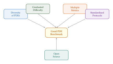
Remark 36 (The benchmark trap).
There is a well-known risk in machine learning of “teaching to the test”: optimising methods for benchmark performance at the expense of genuine scientific utility. In the PDE context, this can manifest as models that achieve low error on smooth benchmark solutions but fail catastrophically on out-of-distribution regimes (higher Reynolds numbers, different geometries, longer time horizons).
The remedy is continuous evolution of benchmarks: as the community solves existing benchmarks, new, harder challenges must be introduced. The progression from PDEBench (2022) to PINNacle (2024) to InverseBench (2025) represents healthy growth in this direction.
| Feature | PDEBench | PINNacle | InverseBench |
| Focus | Data-driven surrogates | PINNs | Inverse problems |
| Number of PDEs | 7 families | 20+ | 5 |
| Spatial dims | 1D, 2D | 1D–3D | 2D |
| Metrics | , MSE | , | PSNR, SSIM, LPIPS |
| Conservation checks | No | No | No |
| Spectral metrics | No | No | No |
| Open-source | Yes | Yes | Yes |
| Year | 2022 | 2024 | 2025 |
Exercise 41 (Designing a benchmark for turbulent flow surrogates).
Suppose you are tasked with creating a benchmark for evaluating generative models applied to 2D turbulent flow.
- (a)
Select three Reynolds numbers spanning laminar, transitional, and fully turbulent regimes. For each, specify the PDE (incompressible Navier–Stokes), domain, boundary conditions, and forcing.
- (b)
Propose a set of at least five evaluation metrics covering pointwise accuracy, spectral fidelity, conservation, and statistical properties. Justify each choice.
- (c)
Define a standardised training protocol: dataset size, resolution, time span, train/validation/test split ratios, and normalisation procedure.
- (d)
Identify at least three potential pitfalls (e.g., data leakage, resolution dependence, evaluation at a single snapshot vs. trajectory-level metrics) and propose mitigations.
- (e)
Discuss how you would handle the evaluation of generative models (which produce distributions, not single predictions). What metrics capture sample quality vs. sample diversity?
Challenge 6 (Building a mini-PDEBench).
Implement a simplified version of PDEBench covering three equations:
- (a)
1D Burgers equation with .
- (b)
2D heat equation with random initial conditions drawn from a Gaussian random field.
- (c)
2D Darcy flow with log-normal permeability.
For each equation:
Generate training and test solutions using a standard numerical solver (e.g., finite differences for Burgers/heat, finite elements for Darcy).
Train a simple FNO and a U-Net baseline.
Evaluate using , , and (for Burgers) conservation residuals.
Store all data in HDF5 with appropriate metadata.
Release your code and data on GitHub.
Insight.
The sections on inverse problems, uncertainty quantification, and benchmarking form a coherent triad: inverse problems demand UQ because the solution is inherently non-unique; UQ demands benchmarks because claimed uncertainties must be validated; and benchmarks demand diverse metrics because no single number captures the quality of a probabilistic PDE solver. Together, they define the infrastructure needed to move neural PDE solvers from proof-of-concept demonstrations to trustworthy, deployable tools.
Open Problems and Future Challenges
“In so far as the laws of mathematics refer to reality, they are not certain; and in so far as they are certain, they do not refer to reality.” - Albert Einstein, 1921
We have now traversed a long path-from the classical PDE solvers of the twentieth century through physics-informed neural networks, neural operators, Transformer-based architectures, and diffusion models on function spaces. The tools are powerful, the progress remarkable, and the pace of discovery exhilarating. Yet the honest truth is that we are still near the beginning. The most profound questions-about turbulence, about guarantees, about the relationship between data-driven and physics-driven understanding-remain wide open.
This section surveys the frontier. We revisit the most famous unsolved problem in mathematical physics, chart the challenges that must be overcome for generative PDE solvers to fulfil their promise, and close with philosophical reflections that we hope will inspire the next generation of researchers.
The Navier–Stokes Millennium Prize Revisited
In Section A First Look at PDEs and Why They Matter we encountered the Navier–Stokes equations and mentioned that the question of their regularity in three dimensions is one of the seven Clay Millennium Prize Problems, carrying a prize of one million US dollars. Now that we have developed the full machinery of generative PDE solvers, we can ask a more pointed question: can machine learning help crack this problem?
The formal statement
Let us state the problem precisely.
Definition 60 (Navier–Stokes Existence and Smoothness Problem).
Consider the three-dimensional incompressible Navier–Stokes equations on : (NS Momentum) where is the velocity field, is the pressure, is the kinematic viscosity, and is a smooth, bounded external force. Given smooth, divergence-free initial data with rapid decay at infinity, either:
At first glance, this problem may seem remote from machine learning. It is a question about the mathematical existence and regularity of solutions, not about their numerical computation. But as we shall argue, there are surprising and potentially transformative connections.
Why 3D is fundamentally different from 2D
The key to understanding why the 3D problem is so hard lies in a single mechanism: vortex stretching. Define the vorticity . Taking the curl of , we obtain the vorticity equation: (Vorticity)
Key Idea.
The Vortex Stretching Mechanism In two dimensions, the vortex stretching term vanishes identically, because is perpendicular to the plane of motion. This makes the 2D Navier–Stokes equations much tamer: global existence and smoothness were proved by Ladyzhenskaya in 1959. In three dimensions, however, vortex tubes can stretch, amplifying vorticity exponentially-and it is unknown whether the viscous dissipation term is always strong enough to prevent the vorticity from blowing up in finite time.
Proposition 27 (Beale–Kato–Majda Criterion).
A smooth solution of the 3D Navier–Stokes equations develops a singularity at time if and only if (BKM) That is, the only way a smooth solution can break down is through the blow-up of the maximum vorticity.
This criterion tells us exactly what to look for: scenarios where the pointwise maximum of vorticity grows without bound.
Partial results: from Leray to the present
Historical Note.
Leray's 1934 masterpiece. In 1934, the French mathematician Jean Leray published a landmark paper that introduced the concept of weak solutions (solutions in an integral sense that may lack classical smoothness) and proved that for any smooth initial data, at least one global weak solution of the 3D Navier–Stokes equations exists. These “Leray–Hopf” weak solutions satisfy the energy inequality Leray's result is over 90 years old, and we still do not know whether his weak solutions are actually smooth. The gap between the existence of weak solutions and the existence of smooth solutions is the essence of the Millennium Prize problem.
Theorem 32 (Conditional Regularity Results (Summary)).
The following conditions, any one of which would suffice to guarantee that a Leray–Hopf weak solution is smooth:
Prodi–Serrin condition: with , .
Vorticity condition: (the Beale–Kato–Majda criterion).
Pressure condition: with , .
One-component regularity: with suitable exponents (various results by Neustupa–Penel, Cao–Titi, and others).
None of these conditions has been verified unconditionally.
Can ML help? Probing near-singular behaviour
Here is where generative models enter the picture. Even if they cannot prove theorems directly, they can serve as extraordinarily powerful experimental tools for probing the landscape of possible Navier–Stokes solutions.
Insight.
Generative Models as Experimental Mathematics The strategy is as follows. Train a conditional generative model (e.g., a diffusion model on function space) to produce 3D velocity fields that approximately solve the Navier–Stokes equations. Then use the model to systematically search for initial conditions that lead to extreme vorticity growth-configurations that come “close” to singularity formation. Even if the model cannot produce a true singularity (which would require infinite resolution), it can identify candidate scenarios that classical high-resolution simulations can then investigate.
Several concrete research directions are emerging:
Diffusion models for extreme vorticity sampling. Train a score-based generative model on the distribution of vorticity fields from turbulent simulations. Condition the model on high values of and sample configurations that push the envelope of vorticity concentration. This is an instance of rare-event sampling using generative models.
AI-assisted conjecture generation. Feed a large language model the corpus of partial regularity results and ask it to propose new conditional regularity criteria-new functional norms or geometric conditions under which smoothness can be guaranteed. The model can suggest candidates; formal theorem provers (see the mathematics chapter) can attempt to verify them.
Learned Lyapunov functionals. A classical approach to proving regularity is to construct a Lyapunov functional (an energy-like quantity that decreases along solutions). Neural networks can be trained to parameterise candidate Lyapunov functionals, with the loss function penalising violations of the monotonicity condition. If a valid Lyapunov functional is found, it constitutes a machine-generated proof of regularity.
Symmetry-aware search. The Navier–Stokes equations have rich symmetry groups (spatial translations, rotations, scaling). Generative models that respect these symmetries (equivariant architectures) can focus the search on genuinely distinct configurations, avoiding redundant exploration of symmetry-related states.
Remark 37.
We should be honest about the limitations. The Millennium Prize problem is a question about the behaviour of solutions at all scales simultaneously, including infinitesimally small ones. Any numerical or neural computation operates on a finite grid and at finite precision. Machine learning can suggest where to look and what to conjecture, but the final proof (or disproof) will almost certainly require new mathematical ideas. The most likely scenario is that AI serves as a powerful telescope-helping mathematicians see patterns that would otherwise be invisible-rather than as the telescope and the astronomer.
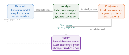
Discretisation-Agnostic Generation
Every method we have studied in this chapter operates, at some level, on a discrete representation: grid points, mesh nodes, spectral coefficients, or tokens. This discretisation is both a practical necessity and a fundamental limitation.
The grid-dependence problem
Consider training a diffusion model on fluid-flow snapshots at resolution . The model learns to generate fields at precisely that resolution. If we need a field-perhaps because a fine-scale feature demands higher resolution-the trained model cannot help. We must retrain on higher-resolution data, which is expensive to generate and requires more GPU memory.
Definition 61 (Discretisation-Agnostic Generative Model).
A generative model for PDE solutions is discretisation-agnostic if, once trained, it can produce samples at any desired spatial or temporal resolution without retraining or fine-tuning. Formally, for any finite set of query points , the model returns consistent marginals: where is a distribution over the infinite-dimensional function space .
Function-space methods as the solution
The key idea is to work directly in function space rather than in for a fixed . We encountered this perspective in the diffusion-on-function-space formulation: the forward process adds noise in a Hilbert space , and the reverse process denoises back to a clean function. The resulting model is, in principle, resolution-independent.
Key Idea.
From Finite Vectors to Infinite Functions The paradigm shift is: Models operating in function space (neural processes, Gaussian neural operators, functional diffusion models) can be queried at arbitrary resolution. The challenge is making them computationally tractable and ensuring that the infinite-dimensional objects are well-defined.
Open questions abound:
Can we define well-posed diffusion processes in infinite-dimensional Hilbert spaces with convergence guarantees for the score-matching objective?
How do we efficiently parameterise score functions on function spaces? Current approaches use discretised approximations-can we avoid this entirely?
What is the correct notion of “distribution” over solutions of a nonlinear PDE? For linear PDEs, Gaussian measures on Sobolev spaces provide a natural framework. For nonlinear PDEs, the situation is far less clear.
Can neural implicit representations (NeRF-like coordinate networks for PDE solutions) achieve true resolution independence, or do they inherit the spectral bias of MLPs?
Real-Time Turbulence and Interactive Simulation
“The goal is not to replace DNS, but to make its insights available in real time.” - Karthik Duraisamy, 2023
For many applications-flight simulators, digital twins of industrial processes, real-time weather nowcasting, interactive surgical planning-the speed of a PDE solver matters as much as its accuracy. Classical high-fidelity solvers deliver accuracy but require hours or days of computation. Generative PDE solvers promise a qualitative leap: from offline batch processing to interactive, real-time simulation.
The 1000 speedup challenge
Definition 62 (Real-Time PDE Solving).
A PDE solver operates in real time for a given application if its wall-clock computation time satisfies where is the physical time span being simulated and is an application-dependent real-time factor. For interactive applications (e.g., flight simulators), is typical (30 fps rendering). For digital twins with control loops, may suffice.
Current state-of-the-art neural surrogates achieve speedups of – over classical solvers for moderate-complexity problems. But for industrially relevant turbulent flows at high Reynolds numbers (), we still fall short of real-time requirements by one to two orders of magnitude.
Latent-space approaches
The most promising path to real-time performance is to operate entirely in a compressed latent space:
Encode the high-dimensional PDE state into a low-dimensional latent vector using a trained encoder.
Evolve the latent state using a lightweight temporal model: . This step is fast because (the number of grid points).
Decode back to the physical state: .
The challenge is ensuring that the latent dynamics respect the physics: conservation laws, stability, and long-time accuracy.
Hardware co-design: neural PDE accelerators
Insight.
Beyond GPUs: Custom Silicon for PDE Solving Just as the rise of deep learning spurred the development of specialised hardware (GPUs, TPUs, Cerebras wafer-scale engines), the rise of neural PDE solvers may eventually motivate custom silicon optimised for the specific computational patterns of operator learning and diffusion-based generation. Imagine a chip that implements the Fourier Neural Operator's spectral convolution natively, achieving orders-of-magnitude speedups over general-purpose GPUs. This is not science fiction: FPGA implementations of neural operators are already being explored in the aerospace industry.
Example 52 (Application Areas for Real-Time Neural PDE Solving).
Digital twins: A virtual replica of a jet engine that runs in real time, ingesting sensor data and predicting remaining useful life under current operating conditions.
Flight simulators: Turbulence response in real time for pilot training, replacing look-up-table approximations with physics-faithful generative models.
Weather nowcasting: Probabilistic 0–6 hour precipitation forecasts at 1,km resolution, updated every 5 minutes.
Surgical planning: Interactive blood-flow simulation through patient-specific arterial geometries, enabling surgeons to explore “what if” scenarios before operating.
Autonomous vehicles: Real-time aerodynamic prediction for control systems, adapting to changing vehicle configurations (windows open, roof rack, etc.).
Generative PDE Foundation Models
“Can we build one model that understands all of physics?” - Animashree Anandkumar, 2024
The success of foundation models in natural language (GPT, Claude, Gemini) and vision (DALL-E, Stable Diffusion) naturally raises the question: can we build a foundation model for PDEs? A single, large, pre-trained model that, given a PDE specification (equations, domain geometry, initial/boundary conditions, material parameters), generates accurate solution fields-without any task-specific fine-tuning.
The vision: one model for all PDEs
Definition 63 (PDE Foundation Model).
A PDE foundation model is a pre-trained generative model that takes as input a complete PDE specification comprising the differential operator , the spatial domain , boundary conditions , initial conditions , and physical parameters , and produces samples from the distribution of solutions. The model is trained on a diverse corpus of PDE families (heat, wave, advection, Navier–Stokes, Maxwell, Schrödinger, elasticity, ) and generalises to unseen PDE types without retraining.
Scaling laws: does more data help?
In language modelling, the “scaling laws” of Kaplan et al. (2020) and Hoffmann et al. (2022) showed that test loss decreases as a power law in model size, dataset size, and compute budget. Do similar scaling laws hold for PDE foundation models?
Proposition 28 (Conjectured Scaling Law for PDE Surrogates).
Let denote the expected relative error of a neural PDE surrogate with parameters trained on PDE solution pairs. Empirical evidence suggests: (Scaling LAW) where are PDE-family-dependent exponents, are critical scales, and is an irreducible error from approximation theory (analogous to the entropy of language). Preliminary experiments suggest and , with significant variation across PDE classes.
Remark 38.
There is a crucial difference from language modelling: for PDEs, the “data” can be generated synthetically by running classical solvers. In principle, the dataset is unlimited. The bottleneck is not data scarcity but data generation cost: a single high-fidelity turbulence simulation can take weeks on a supercomputer. This creates an intriguing optimisation problem: how to allocate a fixed compute budget between generating more training data and training a larger model.
Current state of the art
Several groups have taken first steps towards PDE foundation models:
MPP (Multiple Physics Pretraining, McCabe et al., 2023): Pre-trained on 14 PDE families, demonstrated zero-shot transfer to unseen PDEs, achieving competitive accuracy with specialised models.
Unisolver (Unified PDE Solver with PDE-Conditioned Transformers, 2024): Conditions the Transformer attention mechanism directly on the PDE coefficients via “physics cross-attention,” enabling a single model to handle diverse PDE families.
PROSE-FD (Pre-trained Neural Operator for PDE Families, 2024): Learns symbolic representations of PDE operators and conditions the neural solver on these representations.
PDEformer (2024): Uses a tokenised representation of PDE specifications (akin to a “PDE language”) to condition a Transformer-based solver.
What's missing
Despite these promising beginnings, significant gaps remain:
Caution.
Current PDE foundation models lack:
Theoretical guarantees: No convergence rates, no approximation bounds, no worst-case error estimates.
Physical consistency: Conservation laws are not guaranteed; solutions may violate fundamental physics.
Safety certification: None of these models is certified for deployment in safety-critical systems.
Out-of-distribution detection: When the model encounters a PDE outside its training distribution, it may produce plausible-looking but wildly incorrect solutions without warning.
Compositionality: The models do not “understand” the structure of PDEs; they cannot derive conservation laws from the equations or predict qualitative behaviour changes.
Bridging these gaps is the central challenge for the next decade.
Physical Guarantees and Trustworthiness
If we are to deploy neural PDE solvers in applications where lives or infrastructure are at stake-nuclear reactor safety, aircraft design, climate policy-we need guarantees, not just empirical performance metrics.
Conservation laws
Theorem 33 (Noether's Theorem-Informal Statement).
Every continuous symmetry of a physical system's action functional corresponds to a conserved quantity: time translation invariance gives conservation of energy, spatial translation invariance gives conservation of momentum, rotational invariance gives conservation of angular momentum.
Classical numerical schemes-finite volumes, symplectic integrators, structure-preserving discretisations-are carefully designed to respect these conservation laws exactly (at the discrete level). Neural surrogates, trained by minimising a data-driven loss, generally do not conserve these quantities. The mass, energy, or momentum of a neural solution may drift over long time horizons, leading to physically meaningless predictions.
Example 53 (Energy Drift in Neural Surrogates).
Consider training a neural operator to predict the evolution of an inviscid fluid governed by the Euler equations, which conserve total energy. In a typical experiment, the neural surrogate produces visually convincing solutions for the first time steps, but the total energy drifts by 5–15% over 200 time steps, rendering long-time predictions physically meaningless. A structure-preserving classical solver maintains energy to machine precision over the same time span.
Several approaches are being explored:
Hard constraints: Design the neural architecture so that conservation laws are satisfied by construction. For divergence-free fields, use curl-based parameterisations ; for energy-preserving dynamics, use Hamiltonian neural networks.
Soft constraints: Add conservation-law penalties to the loss function. This is simpler but provides no guarantees: the constraints are satisfied approximately, not exactly.
Projection methods: After each neural prediction, project the output onto the constraint manifold (e.g., onto the space of divergence-free fields). This guarantees satisfaction of the constraint at the cost of additional computation.
Hybrid solvers: Use the neural model for fast prediction and a classical solver for correction, in a predict-correct cycle.
A posteriori error estimation
Definition 64 (Certified Neural Surrogate).
A neural PDE surrogate is certified with respect to a PDE operator if, for each input, it provides both a solution estimate and a computable error bound: where the estimator is efficiently computable and provably reliable (i.e., the bound holds without exception).
The key idea is to exploit the residual: even without knowing the true solution , we can evaluate the PDE residual , which should be zero for a perfect solution. Classical a posteriori error estimation theory relates the norm of the residual to the norm of the error, provided stability estimates for the PDE are available.
Out-of-distribution detection
Key Idea.
Knowing What You Don't Know A trustworthy neural PDE solver must not only produce accurate answers when it can, but also refuse to answer-or at least flag high uncertainty-when the input falls outside its training distribution. This is the “knowing what you don't know” problem, and it is arguably harder for PDE surrogates than for image classifiers, because the input space (PDE specifications) is infinite-dimensional and its structure is poorly understood.
High-Dimensional PDEs and the Curse of Dimensionality
Most of this chapter has focused on PDEs in two or three spatial dimensions-the “natural” setting for fluid dynamics, electromagnetism, and elasticity. But some of the most important PDEs in science and engineering live in much higher dimensions.
Where high-dimensional PDEs arise
Quantum mechanics: The Schrödinger equation for particles lives in spatial dimensions. For a molecule with 100 electrons, this is a PDE in 300 dimensions.
Optimal control and finance: The Hamilton–Jacobi–Bellman (HJB) equation for an optimal control problem with state variables is a PDE in dimensions. Realistic portfolio optimisation problems can have .
Mean-field games: Models of large populations of interacting agents (traffic flow, epidemic spreading, economic markets) lead to coupled systems of high-dimensional PDEs.
Kinetic theory: The Boltzmann equation for a gas lives in 6-dimensional phase space (3 positions + 3 velocities), and its numerical solution is already at the edge of feasibility.
Classical grid-based methods are hopeless in high dimensions: a grid with points per dimension requires total points, which exceeds the number of atoms in the observable universe for and . This is the infamous curse of dimensionality.
Deep BSDE methods
One of the most striking success stories of deep learning for PDEs is the deep BSDE method of E, Han, and Jentzen (2017), which exploits a beautiful connection between parabolic PDEs and stochastic processes.
Theorem 34 (Feynman–Kac Formula-Informal).
The solution of a parabolic PDE can be represented as the conditional expectation where is the diffusion process .
The deep BSDE method parameterises the gradient at each time step by a neural network and optimises the terminal condition along sampled stochastic trajectories. Crucially, the method's computational cost scales polynomially in dimension -breaking the curse of dimensionality.
Insight.
The SDE–PDE Duality and Diffusion Models There is a deep and beautiful symmetry here. Diffusion-based generative models work by converting a data distribution into noise via a forward SDE, then learning to reverse the process. The deep BSDE method works by converting a PDE problem into a forward SDE problem, then learning the gradient along trajectories. Both exploit the Feynman–Kac duality between PDEs and stochastic processes. This suggests a unified framework: a generative diffusion model that simultaneously solves high-dimensional PDEs and generates samples from complex distributions. Building this unification rigorously is an open problem.
The potential of generative models
Can generative models go further than the deep BSDE method? Several tantalising directions exist:
Score-based solvers for HJB equations: The Hamilton–Jacobi–Bellman equation can be viewed as defining a score function (the gradient of the value function) on a high-dimensional state space. Score-based generative models are designed precisely to learn such gradients-can they be repurposed as HJB solvers?
Mean-field generative models: For mean-field games, the coupled PDE system involves a forward Fokker–Planck equation and a backward HJB equation. A generative model could learn the joint distribution of trajectories, from which both the density and the value function can be extracted.
Quantum many-body wavefunctions: The Schrödinger equation for many particles is a high-dimensional PDE. Recent work (PauliNet, FermiNet, DiffusionQMC) uses neural networks to represent many-body wavefunctions. Generative models could sample from the Born probability distribution directly.
Climate and Weather: The Ultimate Test
“Prediction is very difficult, especially if it's about the future.” - Niels Bohr (attributed)
If there is one domain where the promise and peril of generative PDE solvers converge with maximum intensity, it is weather and climate prediction. The atmosphere is governed by the Navier–Stokes equations coupled with thermodynamics, radiation transfer, moisture transport, and ocean-atmosphere interaction. The system is chaotic, multi-scale, and of existential importance to humanity.
Weather prediction as a PDE problem
Numerical Weather Prediction (NWP) has been one of the great scientific and computational achievements of the twentieth century. The basic approach-discretise the atmospheric equations on a global grid and time-step them forward-has been refined over 70 years at operational centres like ECMWF, NOAA, and the Met Office. The current state of the art, ECMWF's IFS (Integrated Forecasting System), uses a spectral transform method at roughly 9,km horizontal resolution with 137 vertical levels, producing 51-member ensemble forecasts that take approximately one hour of wall-clock time on a dedicated supercomputer.
The AI weather revolution
In 2022–2024, a series of landmark results showed that AI models can match or exceed the accuracy of IFS for medium-range weather forecasting:
Pangu-Weather (Huawei, 2023): A 3D Swin Transformer trained on 39 years of ERA5 reanalysis data, producing 5-day global forecasts in seconds.
GraphCast (DeepMind, 2023): A graph neural network operating on an icosahedral mesh, achieving state-of-the-art accuracy on 90% of 1,380 verification targets.
GenCast (DeepMind, 2024): A conditional diffusion model that generates probabilistic ensemble forecasts, providing not just a single prediction but a distribution over possible weather outcomes. GenCast outperformed ECMWF's operational ensemble on probabilistic skill metrics.
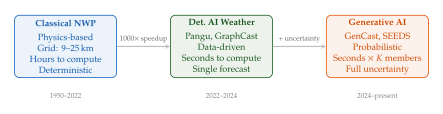
Climate modelling: the century-scale challenge
Weather prediction operates on a time horizon of days to weeks. Climate modelling asks a much harder question: what will the statistical distribution of weather look like decades or centuries from now, under different greenhouse gas emission scenarios?
This is a problem of a fundamentally different character. Weather prediction is an initial-value problem (given today's atmospheric state, predict tomorrow's). Climate modelling is a boundary-value problem in the space of forcing scenarios: given a trajectory of CO concentrations, predict the long-term statistical equilibrium of the climate system.
Exercise 42.
Explain the fundamental difference between weather prediction and climate projection in terms of initial-value problems vs. boundary-value problems. Why does skill at weather prediction not automatically imply skill at climate projection? Hint: Think about sensitivity to initial conditions vs. sensitivity to boundary conditions.
Remark 39.
Generative models for climate have an additional ethical dimension. If an AI model produces century-scale climate projections that diverge from established physics-based models, the implications for policy could be enormous. Overconfident AI predictions could lead to either dangerous complacency or unnecessary alarm. Any AI climate model must be thoroughly validated against the understood physics and against the historical record-and its limitations must be communicated transparently to policymakers.
A Grand Challenge: Twenty Open Questions
“The formulation of a problem is often more essential than its solution, which may be merely a matter of mathematical or experimental skill.” - Albert Einstein
We now present twenty concrete open research questions. They range from deep theoretical problems that may take decades to resolve, to practical engineering challenges that a determined team could tackle in a year. We have marked each question with a difficulty rating: -1pt[defblue] (0,0) circle (3pt); for problems accessible to motivated undergraduates, -1pt[exorange] (0,0) circle (3pt);[exorange] (8pt,0) circle (3pt); for PhD-level research, and -1pt[exrcoral] (0,0) circle (3pt);[exrcoral] (8pt,0) circle (3pt);[exrcoral] (16pt,0) circle (3pt); for “Millennium Prize”-level challenges.
I. Theoretical Foundations
Convergence of function-space diffusion. -1pt[exorange] (0,0) circle (3pt);[exorange] (8pt,0) circle (3pt); Prove that score-matching in infinite-dimensional Hilbert spaces converges to the true score as the number of training samples and network capacity grow. What are the rates?
Approximation theory for neural operators. -1pt[exorange] (0,0) circle (3pt);[exorange] (8pt,0) circle (3pt); Determine tight upper and lower bounds on the number of parameters needed for a neural operator to approximate a solution map to within error. How do these bounds depend on the smoothness and nonlinearity of the PDE?
Navier–Stokes regularity via learned Lyapunov functionals. -1pt[exrcoral] (0,0) circle (3pt);[exrcoral] (8pt,0) circle (3pt);[exrcoral] (16pt,0) circle (3pt); Can a neural network discover a Lyapunov-type energy functional that proves global regularity (or yields a finite-time blow-up scenario) for the 3D Navier–Stokes equations?
Generative models and ergodic theory. -1pt[exorange] (0,0) circle (3pt);[exorange] (8pt,0) circle (3pt); For chaotic PDEs (e.g., turbulent Navier–Stokes), the long-time statistics are governed by an invariant measure. Can a diffusion model learn this invariant measure, and if so, does sampling from the model produce trajectories with the correct ergodic properties?
Complexity of PDE solving with neural networks. -1pt[exrcoral] (0,0) circle (3pt);[exrcoral] (8pt,0) circle (3pt);[exrcoral] (16pt,0) circle (3pt); Is there a complexity-theoretic separation between neural PDE solvers and classical solvers? Can neural networks solve certain PDE families in polynomial time (in dimension) where classical grid methods require exponential time?
II. Architectures and Methods
Equivariant diffusion on function spaces. -1pt[exorange] (0,0) circle (3pt);[exorange] (8pt,0) circle (3pt); Design a diffusion model on function space that is equivariant to the full symmetry group of the PDE (spatial translations, rotations, Galilean boosts, scaling). Does symmetry equivariance improve sample quality and data efficiency?
Autoregressive vs. diffusion for temporal rollouts. -1pt[defblue] (0,0) circle (3pt); Systematically compare autoregressive (one-step-at-a-time) and diffusion-based (full-trajectory) generation for time-dependent PDEs. Under what conditions does each approach dominate?
Latent-space dynamics with physical constraints. -1pt[exorange] (0,0) circle (3pt);[exorange] (8pt,0) circle (3pt); Develop an encoder-decoder architecture for PDE states where the latent dynamics provably conserve energy, momentum, and mass. Can symplectic or Hamiltonian structures be imposed in the latent space?
Tokenisation of PDE specifications. -1pt[defblue] (0,0) circle (3pt); What is the optimal way to represent a PDE specification (equations, domain, boundary conditions) as a sequence of tokens for a Transformer? Can symbolic tokenisation (parsing the PDE into an abstract syntax tree) outperform naive string tokenisation?
Multi-fidelity generative training. -1pt[defblue] (0,0) circle (3pt); Train a generative PDE model on a mix of cheap low-resolution and expensive high-resolution simulation data. Can multi-fidelity training achieve the accuracy of high-fidelity training at a fraction of the data-generation cost?
III. Applications and Deployment
Certified neural surrogates for nuclear safety. -1pt[exorange] (0,0) circle (3pt);[exorange] (8pt,0) circle (3pt); Develop a neural PDE surrogate for reactor thermal-hydraulics that comes with provable error bounds sufficient for regulatory certification.
Real-time turbulence for flight simulation. -1pt[exorange] (0,0) circle (3pt);[exorange] (8pt,0) circle (3pt); Build a generative model that produces realistic turbulent flow fields around an aircraft at interactive frame rates (,fps), with statistical properties matching high-fidelity LES or DNS within specified tolerances.
Generative climate emulators. -1pt[exorange] (0,0) circle (3pt);[exorange] (8pt,0) circle (3pt); Train a generative model that produces physically consistent century-scale climate trajectories conditioned on emission scenarios, matching the statistical behaviour of CMIP6 models but running faster.
Inverse design with generative PDE solvers. -1pt[defblue] (0,0) circle (3pt); Use a conditional diffusion model to solve inverse design problems: given a desired flow property (e.g., minimum drag), generate the geometry that achieves it. Compare with classical adjoint-based optimisation.
Patient-specific surgical planning. -1pt[exorange] (0,0) circle (3pt);[exorange] (8pt,0) circle (3pt); Build a generative cardiovascular flow solver that takes a patient's CT/MRI-derived vascular geometry, produces an ensemble of possible haemodynamic scenarios, and runs fast enough for intraoperative use.
IV. Benchmarks and Evaluation
A unified benchmark for generative PDE solvers. -1pt[defblue] (0,0) circle (3pt); Create a comprehensive benchmark suite (analogous to ImageNet for vision or GLUE for NLP) covering diverse PDE families, geometries, and evaluation metrics, with standardised train/test splits and evaluation protocols.
Perceptual metrics for PDE solutions. -1pt[defblue] (0,0) circle (3pt); Pointwise error fails to capture the perceptual quality of turbulent flow fields (analogous to how MSE fails for images). Develop physically motivated perceptual metrics that assess the statistical, spectral, and structural fidelity of generated PDE solutions.
Stress-testing out-of-distribution. -1pt[defblue] (0,0) circle (3pt); Systematically characterise the failure modes of neural PDE solvers under distribution shift: changes in Reynolds number, domain geometry, boundary conditions, and PDE coefficients. Build a “breaking point” dataset.
V. Connections and Unifications
PDE solving as language modelling. -1pt[exorange] (0,0) circle (3pt);[exorange] (8pt,0) circle (3pt); Is there a meaningful sense in which PDE solutions can be “narrated” as sequences, and autoregressive language models can serve as PDE solvers? What are the theoretical limitations of this analogy?
The grand unification: one model for science. -1pt[exrcoral] (0,0) circle (3pt);[exrcoral] (8pt,0) circle (3pt);[exrcoral] (16pt,0) circle (3pt); Can we build a single foundation model that simultaneously handles fluid dynamics, solid mechanics, electromagnetism, quantum mechanics, and their couplings? What are the fundamental obstacles-architectural, data-related, or information-theoretic-to such a model?
Exercise 43.
Choose one of the twenty open questions above and write a 2-page research proposal outlining: (a) the precise problem formulation, (b) your proposed approach, (c) the expected difficulties, and (d) how you would evaluate success. This is excellent practice for writing real research proposals.
Philosophical Reflections
“The miracle of the appropriateness of the language of mathematics for the formulation of the laws of physics is a wonderful gift which we neither understand nor deserve.” - Eugene Wigner, 1960
We close this chapter-and this part of the book-with some reflections that are more philosophical than technical. They are offered not as definitive answers but as invitations to thought.
Does a Neural PDE Solver “Understand” Physics?
When a Fourier Neural Operator produces a flow field that matches DNS to within 2% relative error, does it “understand” fluid mechanics? The question may seem idle, but it has practical implications.
Consider two scenarios:
A student who memorises the answers to every problem in a fluid mechanics textbook without understanding the derivations. Ask them a problem they have seen before, and they answer correctly. Ask them a genuinely novel problem, and they fail.
A student who understands the Navier–Stokes equations deeply-the role of each term, the physical mechanisms, the dimensional analysis. They may not have memorised any answers, but they can derive solutions to problems they have never seen.
Current neural PDE solvers are closer to the first student. They excel at interpolation (problems “between” training examples) but struggle at extrapolation (problems genuinely outside the training distribution). A model trained on flows at Reynolds numbers to may fail catastrophically at .
Key Idea.
Understanding vs. Pattern Matching We propose a practical definition: a neural PDE solver “understands” a physical phenomenon to the extent that it can extrapolate correctly to regimes not seen during training. By this criterion, current models have limited understanding. The quest for genuine physical understanding in neural networks is closely connected to the quest for compositional generalisation: the ability to combine learned primitives in novel ways.
Data-Driven vs. Physics-Driven: The Central Tension
The field of scientific machine learning is animated by a fundamental tension between two philosophies:
The data-driven philosophy: “Let the data speak. Given enough data and a sufficiently flexible model, the physics will emerge automatically. We do not need to encode physical laws; the model will discover them.”
The physics-driven philosophy: “Physical laws are hard-won distillations of centuries of human understanding. Ignoring them is wasteful and dangerous. Encode them into the model architecture and loss function; use data only to fill in what physics alone cannot determine.”
The truth, as usual, lies somewhere in between-but the optimal balance is far from obvious and likely depends on the application.
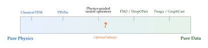
Historical Note.
The two cultures. This tension echoes an older debate in statistics. In 2001, Leo Breiman published a provocative paper entitled “Statistical Modelling: The Two Cultures,” contrasting data-modelling (assuming a generative process and fitting parameters) with algorithmic modelling (using flexible models like random forests to predict without assumptions). Breiman argued that the algorithmic culture was undervalued. Twenty-five years later, the pendulum has swung dramatically: data-driven methods dominate many benchmarks. But for physical systems, where we have strong prior knowledge in the form of conservation laws and symmetries, the question of how to incorporate this knowledge remains critical.
Symbolic AI vs. Connectionist AI for Scientific Discovery
The tension between physics-driven and data-driven approaches is a specific instance of a much older debate in artificial intelligence: symbolic vs. connectionist AI.
Symbolic AI-exemplified by expert systems, theorem provers, and symbolic regression-represents knowledge as explicit rules and manipulates them logically. Connectionist AI-exemplified by neural networks-represents knowledge as distributed patterns of activation in high-dimensional weight spaces.
For scientific discovery, the ideal would be a system that combines:
The generalisation and pattern recognition abilities of connectionist models (finding structure in vast datasets that no human could survey);
The interpretability and compositionality of symbolic models (producing results that humans can understand, verify, and build upon);
The rigour of formal mathematical proof (ensuring that discovered relationships are not just correlations but provable truths).
Remark 40.
The integration of these three capabilities is the central challenge of “AI for Science.” Some recent systems-notably those combining LLMs with formal theorem provers-take steps in this direction. But a truly unified neuro-symbolic-formal system for scientific discovery remains a distant goal.
Two Kinds of Unreasonable Effectiveness
In 1960, the physicist Eugene Wigner published his celebrated essay The Unreasonable Effectiveness of Mathematics in the Natural Sciences. He marvelled at the fact that abstract mathematical structures-developed by pure mathematicians with no physical application in mind-turn out, again and again, to be precisely the right language for describing physical reality. Riemannian geometry, conceived in the abstract, turned out to be the language of general relativity. Group theory, developed for its own beauty, became the foundation of particle physics.
Six decades later, we face an analogous puzzle: the unreasonable effectiveness of deep learning. Neural networks-universal function approximators with no built-in physical knowledge-turn out to be extraordinarily effective at learning the solutions of PDEs. A generic architecture (Transformer, U-Net) trained on examples can match or exceed decades of domain-specific numerical method development.
Conjecture 4 (The Double Effectiveness Hypothesis).
The effectiveness of mathematics for physics and the effectiveness of deep learning for PDE solving are not unrelated coincidences but manifestations of a shared underlying principle: both exploit compositionality and symmetry in the structure of physical laws. Mathematics is effective because physical laws are compositional (complex phenomena emerge from simple, symmetric building blocks). Deep learning is effective because neural networks are universal approximators of compositional functions, and their inductive biases (locality in CNNs, attention in Transformers) align with the compositional structure of physics.
The Role of Human Intuition in an AI-Augmented World
Perhaps the most important question of all is not technical but human: in a world where AI can solve PDEs faster and more accurately than humans, what is the role of human intuition?
We believe the answer is: more important than ever.
Insight.
The Augmented Scientist AI does not replace the need for physical intuition-it amplifies it. When a classical simulation took weeks, a scientist could test only a handful of hypotheses. When a generative model produces solutions in seconds, the bottleneck shifts from computation to imagination: which questions to ask, which parameter regimes to explore, which anomalies to investigate. The scientist who combines deep physical intuition with fluency in AI tools will be vastly more productive than either the pure theorist or the pure ML engineer.
The history of science suggests that the greatest discoveries occur not when a tool replaces human thought but when it extends it. The telescope did not replace the astronomer; it gave the astronomer new eyes. The computer did not replace the mathematician; it gave the mathematician new hands. Generative PDE solvers will not replace the physicist or engineer; they will give them new powers of exploration.
Exercise 44.
Write a short (1-page) science fiction scenario set in 2040 in which a researcher uses a generative PDE foundation model to make a major scientific discovery. What role does human intuition play in the story? What role does the AI play? How do they complement each other?
0.50.4pt
“We stand at the beginning of a new relationship between humans and the mathematical laws that govern the physical world. For three centuries, we have used our minds to derive solutions; for seventy years, we have used our computers to approximate them. Now, for the first time, we can learn them. The question is not whether AI will transform computational physics-it already has. The question is whether we will be wise enough to wield this power with the care it demands, and bold enough to ask the questions it makes possible.”
We close with a grand challenge and a conjecture, offered in the spirit of Hilbert's 1900 address and the Clay Millennium Problems, as a beacon for the next generation.
Challenge 7.
The Generative PDE Grand Challenge. Build a single generative model that, given any well-posed PDE specification (equation, domain, initial/boundary conditions, parameters), produces physically consistent solution fields with certified error bounds, at a computational cost that is polynomial in the spatial dimension and independent of the grid resolution. Demonstrate the model on at least five fundamentally different PDE families (including at least one in dimension ), and show that its solutions respect the conservation laws implied by the PDE's symmetries.
Conjecture 5 (The Physics–Learning Duality).
There exists a formal duality between structure-preserving numerical methods for PDEs (symplectic integrators, divergence-free discretisations, entropy-stable schemes) and inductive biases in neural architectures (equivariance, conservation layers, Hamiltonian networks). Specifically, for every class of structure-preserving numerical method, there is a corresponding class of neural architecture that achieves the same conservation properties with provably fewer parameters; and conversely, every conservation-respecting neural architecture implicitly implements a structure-preserving discretisation of the underlying PDE. Establishing this duality rigorously would unify classical numerical analysis and geometric deep learning into a single theoretical framework.
“The important thing is not to stop questioning. Curiosity has its own reason for existence.” - Albert Einstein
This is not the end. It is not even the beginning of the end. But it is, perhaps, the end of the beginning.
Pen-and-Paper Exercises
The exercises in this section are designed to solidify the theoretical foundations developed throughout the chapter. They range from straightforward calculations (3570END) to demanding proofs that require combining ideas from multiple sections (3571END). We encourage the reader to attempt each exercise before consulting any hints, and to write complete, rigorous solutions.
Key Idea.
Difficulty Ratings Throughout this section we use a star rating to indicate difficulty: = direct computation or definition check; = requires combining two ideas; = requires a short proof or careful calculation; = demands significant technical sophistication; = research-level, open to creative approaches.
Exercise 45 (PDE Classification).
3577END Classify each of the following second-order linear PDEs in two variables as elliptic, parabolic, or hyperbolic by computing the discriminant of the principal part:
.
.
.
.
(interpret as a PDE in with as a parameter vs. as a PDE in ).
For each case, state whether the PDE is well-suited to steady-state, initial-value, or boundary-value formulations, and briefly explain why.
Exercise 46 (PINN Loss for the Heat Equation).
3587END Consider the one-dimensional heat equation on : (HEAT) with and .
Write down the full PINN loss explicitly, identifying each term.
Compute the exact solution and verify it satisfies (HEAT).
Using the exact solution, show that for any MLP , the PDE residual loss is exactly zero if and only if satisfies the heat equation pointwise at the collocation points.
Discuss what happens to the training dynamics if , and conversely if .
Exercise 47 (PINN Loss for the Wave Equation).
3599END Derive the PINN loss function for the one-dimensional wave equation: with , , and homogeneous Dirichlet boundary conditions.
Write down each component of the composite loss, noting that the initial condition now involves two constraints (displacement and velocity).
The wave equation has characteristic speed . Explain, using the notion of a domain of dependence, why PINNs with uniform random collocation tend to struggle with sharp wave fronts.
Propose a modified sampling strategy for the collocation points that could mitigate this issue.
Hint: Think about how causal training (The core idea) addresses temporal causality.
Exercise 48 (PINN Loss for Burgers' Equation).
3604END The viscous Burgers' equation is:
Write down the PINN residual . Note which derivatives must be computed via automatic differentiation.
Show that the nonlinear term requires careful treatment: compute the total number of backward passes needed to evaluate at a single collocation point.
For , sketch (qualitatively) the expected solution profile at , explaining the formation of a steep gradient. Why does this steep gradient cause difficulty for PINNs?
Exercise 49 (Properties of the Fourier Neural Operator Kernel).
3611END Recall that the Fourier layer in the FNO applies the update (FNO Layer) where the integral operator is defined via with being the learnable frequency-domain weights, the discrete Fourier transform (DFT) of , and a frequency cutoff.
Show that is a linear integral operator: i.e., .
Prove that the kernel is translation-invariant (i.e., depends only on ).
Show that truncating to modes is equivalent to projecting onto a finite-dimensional subspace of , and estimate the approximation error in terms of the Fourier decay rate of .
If (a Sobolev space of regularity ), show that the truncation error is .
Hint: For part (d), recall that implies for some constant .
Exercise 50 (Attention Approximates Integral Operators).
3632END Consider a general integral operator on functions : where is a kernel function.
Write the softmax attention mechanism as a discretised integral operator over , identifying the kernel .
Show that as the number of discretisation points , the attention output converges (under mild regularity conditions) to the integral with a normalised kernel.
Prove that this normalised kernel satisfies for all , making it a Markov-type kernel.
Discuss the implications for learning Green's functions of PDEs: what symmetry properties of the true Green's function are not naturally captured by softmax attention?
Hint: For part (d), recall that Green's functions of self-adjoint operators satisfy .
Exercise 51 (Score of a Gaussian Field).
3645END Let be a zero-mean Gaussian random field on discretised on a uniform grid of points, yielding a vector with where is a squared-exponential covariance.
Write down the probability density and compute the score function .
Show that the score is linear in : .
For the forward diffusion process , derive the score of the noised distribution and show it takes the form .
Discuss why this closed-form result is useful for sanity-checking score-based diffusion models on PDE solution distributions.
Exercise 52 (Kolmogorov Microscale Computation).
3659END The Kolmogorov microscale is , where is the kinematic viscosity and is the turbulent dissipation rate. For homogeneous isotropic turbulence in a periodic box of side with integral-scale Reynolds number (where is the rms velocity fluctuation), the dissipation scales as .
Show that .
Compute for: itemize
(low turbulence, lab scale),
(moderate turbulence),
(atmospheric boundary layer), itemize assuming in each case.
For DNS on a periodic box, the grid spacing must satisfy . In three dimensions, show that the total number of grid points scales as and compute for each of the above Reynolds numbers.
Estimate the wall-clock time for each DNS if a single time-step costs seconds and the simulation requires time-steps. Use this to argue that DNS at atmospheric Reynolds numbers is intractable.
Exercise 53 (The Cole–Hopf Transformation).
3678END The Cole–Hopf transformation converts the nonlinear Burgers' equation into the linear heat equation. Let satisfy
Define . Show that .
Substitute into Burgers' equation and show that satisfies the heat equation .
Starting from the initial condition on , write down (without solving) the initial condition for and explain how the exact Burgers' solution can be recovered.
Discuss why this analytical technique does not generalise to higher-dimensional or non-integrable PDEs, motivating the need for neural network-based approaches.
Exercise 54 (Deriving the Stefan Condition).
3689END Consider a one-dimensional phase-change problem where a material occupies and melts at temperature . The solid–liquid interface is at , with temperature fields in the solid () and in the liquid (), each satisfying the heat equation in their respective domains.
By considering conservation of energy across the interface, derive the Stefan condition: where is the density, is the latent heat, and , are the thermal conductivities.
Explain why this moving-boundary problem poses a challenge for standard PINNs (which assume a fixed domain).
Propose a neural network architecture that could handle the moving boundary by parameterising both the temperature fields and the interface location.
Hint: For part (a), integrate the heat equation across a thin strip and take .
Exercise 55 (Antisymmetry of Slater Determinants).
3704END In quantum mechanics, an -electron wavefunction must be antisymmetric under exchange of any two electrons. The Slater determinant constructs such a wavefunction from single-particle orbitals :
Prove that is antisymmetric: swapping (for ) gives .
Show that if for some , then (the Pauli exclusion principle).
Explain why neural network architectures for quantum many-body PDEs (such as FermiNet and PauliNet) must build in this antisymmetry structurally, and how a Slater-determinant backbone achieves this.
Exercise 56 (Function-Space Forward SDE).
3715END In a function-space diffusion model, we define a forward process on fields via the SDE: (FUNC SDE) where is a cylindrical Wiener process on and is a noise schedule.
Show that the marginal distribution at time , starting from a deterministic field , is Gaussian: , where and is the identity operator.
Explain why the use of a cylindrical Wiener process (rather than a trace-class process) leads to samples that are only distributions (generalised functions), not smooth fields. What practical consequences does this have for discretisation?
If we instead use a coloured noise for some trace-class covariance operator , derive the marginal distribution and show that the terminal distribution is rather than white noise.
Discuss the trade-off: coloured noise preserves regularity but requires knowledge of . Propose a practical scheme for choosing from training data.
Hint: For part (a), write the Ornstein–Uhlenbeck solution in integral form and compute the first two moments.
Exercise 57 (Grid Points for Direct Numerical Simulation).
3731END For DNS of three-dimensional homogeneous turbulence:
Verify that the number of grid points per direction is , so the total three-dimensional grid has points.
The CFL condition requires . Assuming and , show that the number of time-steps for a simulation of duration (one large-eddy turnover time) is .
Conclude that the total computational cost (proportional to ) scales as .
Fill in the following table:
Express answers in scientific notation.Cost (relative) Lab scale ? ? ? Wind tunnel ? ? ? Atmosphere ? ? ? Astrophysical ? ? ?
Exercise 58 (FNO Zero-Shot Super-Resolution).
3748END A key property of the FNO is that it can be trained at one resolution and evaluated at a different (typically higher) resolution without retraining. This is called zero-shot super-resolution.
Explain why this property follows from the fact that the FNO parameterises its kernel in Fourier space with a fixed set of modes . Show that the learned weights can be applied unchanged when the DFT is computed on a finer grid.
Suppose the FNO is trained on grids of size . If we evaluate on a grid of size , what happens to the Fourier modes ? Are they zero, or do they carry information?
Prove that if the underlying solution and the FNO has modes, then the super-resolution error is bounded by the sum of (i) the training-resolution approximation error and (ii) an aliasing term of order .
DeepONet does not enjoy zero-shot super-resolution by default. Explain why, in terms of its trunk-net architecture.
Exercise 59 (Neural Tangent Kernel Spectral Bias for PINNs).
3757END Consider a two-layer network with and random initialisation , .
Compute the Neural Tangent Kernel (NTK) at initialisation and show it converges (as ) to .
Compute the eigenvalues of on numerically (or argue qualitatively about their decay rate). Show that high-frequency eigenfunctions have small eigenvalues.
Recall that gradient descent on the squared loss converges exponentially in each eigendirection at rate . Conclude that PINNs learn low-frequency components of the PDE solution much faster than high-frequency components (the “spectral bias”).
Discuss how Fourier feature embeddings with large can mitigate spectral bias by reshaping the NTK spectrum.
Exercise 60 (Causal Training Weights and Monotonicity).
3771END In the causal training formulation for PINNs, the loss at time is weighted by (Causal Weights) where is the PDE residual loss at the -th time slice and is a steepness parameter.
Show that and for all , i.e., the weights are monotonically non-increasing.
Prove that if for all (the PDE is satisfied exactly at earlier times), then , so the loss at time is given full weight.
Conversely, show that if is large, then , effectively ignoring future time slices until earlier ones are resolved.
Interpret this mechanism in terms of the “causal structure” of time-dependent PDEs and explain why it prevents the optimizer from fitting the solution at late times before getting early times correct.
Describe what happens in the limits and .
Exercise 61 (Break-Even: Neural Operators vs. FEM).
3788END Suppose a finite element solver requires time to solve a PDE on a mesh with degrees of freedom, where is a hardware-dependent constant. A neural operator has:
Offline training cost: , where is the number of training samples, is the number of epochs, and is a constant.
Online inference cost per query: .
Derive the break-even number of queries above which the neural operator is cheaper than running the FEM solver times. That is, find such that .
Compute for , , , , , . Is the break-even point practical for engineering design-space exploration?
How does scale with ? At what problem size does the neural operator become most advantageous?
Discuss factors this simple model ignores (accuracy degradation, GPU vs. CPU differences, data generation cost, etc.).
Exercise 62 (DeepONet and the Universal Approximation Theorem for Operators).
3810END The universal approximation theorem for operators (Chen & Chen, 1995) states that any continuous operator can be approximated to arbitrary accuracy by a network of the form where are fixed sensor locations, are continuous functions, and are continuous functions of the output coordinate.
Explain why this architecture can be viewed as a finite-rank approximation to the operator , with rank .
Show that if is a linear operator (e.g., the solution operator of a linear PDE), then the branch outputs can be chosen as linear functions of the sensor values.
Discuss the limitation: the sensor locations are fixed at training time. Why does this prevent straightforward super-resolution, and how do recent “continuous sensor” extensions address this?
Contrast DeepONet's approximation-theoretic guarantee with the FNO's: which architecture provides stronger guarantees for operators with translation-invariant kernels, and why?
Exercise 63 (Denoising Score Matching on Discretised Fields).
3821END Let be a dataset of discretised PDE solutions, each (values on an -point grid). A score network is trained with the denoising score matching loss: (DSM)
Show that the optimal score network satisfies .
If comes from a distribution supported on smooth functions (e.g., for large ), argue that the score at small noise levels concentrates near a lower-dimensional manifold in .
Discuss the implications for architecture choice: why might a U-Net (which respects spatial locality) or an FNO (which operates in frequency space) be more appropriate than a generic MLP as the backbone for ?
Exercise 64 (Variational Formulation of Causal PINNs).
3833END Consider the loss functional over the time domain : where is the PDE residual and is a non-negative weight function.
Show that if (standard PINN), then the optimizer may reduce at late times while ignoring early times, violating causality.
Define (the continuous analogue of (Causal Weights)). Show that whenever .
Prove that in the limit , the causal loss converges to a time-stepping scheme: only the earliest time at which receives nonzero weight.
Show that this limit recovers the sequential-in-time training strategy where we solve on first, then , and so on.
Hint: For part (c), use the fact that for any as .
Insight.
Connecting Exercises to Practice The pen-and-paper exercises above establish the mathematical scaffolding for the coding projects that follow. In particular: the PINN loss derivations (Exercises Exercise 46–Exercise 48) are directly implemented in Project Exercise 65; the FNO kernel analysis (Exercise 49) underpins Project Exercise 66; and the score function derivation (Exercise 51) is essential for Projects Exercise 68 and Exercise 73.
Coding Projects
The following projects are designed to be completed in two to four weeks each, assuming familiarity with PyTorch (or JAX) and basic numerical PDE methods. Each project specifies the expected deliverables, suggested architecture, and evaluation criteria. Projects marked with require GPU access; all others can be completed on a laptop CPU (though GPU acceleration is always welcome).
Key Idea.
Project Infrastructure All projects assume the following common infrastructure:
Framework: PyTorch 2.0 or JAX 0.4.
Visualisation: Matplotlib for 1D/2D plots; optionally Plotly for interactive 3D visualisation.
Data: Unless stated otherwise, training data should be generated using a reference solver (e.g.,
scipy.integrate, spectral methods, or PDEBench datasets).Reproducibility: Fix random seeds and report all hyperparameters.
Exercise 65 (PINN for the 2D Heat Equation ).
3856END Goal: Implement a Physics-Informed Neural Network to solve the two-dimensional heat equation with initial condition and homogeneous Dirichlet boundary conditions.
Architecture:
MLP with 4 hidden layers of width 64,
tanhactivations.Input: . Output: .
Use Xavier initialisation for all weight matrices.
Tasks:
Implement the PINN loss with interior collocation points (sampled uniformly), boundary points, and initial condition points.
Train using Adam for iterations with learning rate , then L-BFGS for fine-tuning.
Compare the PINN solution against the exact solution for .
Experiment with loss weights and document the effect on accuracy.
Add Fourier feature embeddings with and random , and compare convergence speed.
Deliverables:
Convergence curves (loss vs. iteration) for all experiments.
Heat maps of at .
Pointwise error maps at the same time snapshots.
Table of relative errors: .
Exercise 66 (FNO for the 1D Burgers Equation ).
3878END Goal: Build and train a Fourier Neural Operator (FNO) that maps initial conditions to solutions of the 1D viscous Burgers equation at time , and test its zero-shot super-resolution capability.
Data generation:
Generate initial conditions on with periodic boundary conditions, where is a Matérn- kernel with length-scale .
Solve each instance using a pseudo-spectral method on a -point grid with .
Downsample to points for training.
Architecture:
4 Fourier layers with modes, hidden width .
Lifting layer: pointwise MLP from to .
Projection layer: pointwise MLP from to .
GeLU activations after each Fourier layer.
Tasks:
Train the FNO on -point data for epochs with the relative loss.
Evaluate on held-out test data () at the training resolution ().
Zero-shot super-resolution: Without retraining, evaluate the same model on -point and -point grids. Report how the relative error changes.
Ablation: vary and plot test error vs. .
Compare against a purely convolutional baseline (U-Net) and show the U-Net fails at super-resolution.
Deliverables:
Training curves and test errors at all resolutions.
Visualisation of 5 predicted vs. ground-truth solutions.
Super-resolution comparison figure (FNO vs. U-Net at points).
Ablation table for .
Exercise 67 (DeepONet for the Parametric Poisson Equation).
3907END Goal: Implement a DeepONet to learn the solution operator of the Poisson equation on with homogeneous Dirichlet boundary conditions.
Data:
Generate random source terms with random coefficients and modes.
Solve using a spectral method (exact for this basis) on a grid.
Architecture:
Branch net: MLP taking sensor values at fixed sensor locations (uniform grid), outputting with .
Trunk net: MLP taking and outputting .
Prediction: .
Tasks:
Train the DeepONet on the MSE loss with training pairs and for validation.
Evaluate generalisation to source terms not in the training set.
Experiment with the number of trunk/branch basis functions and the number of sensor points .
Compare against the FNO (adapted for this problem) in terms of accuracy and inference speed.
Deliverables:
Scatter plots of predicted vs. true solution values.
Relative error distribution over the test set (histogram).
Ablation study over and .
Exercise 68 (Diffusion Model for 1D PDE Solution Fields ).
3931END Goal: Train a denoising diffusion probabilistic model (DDPM) to generate samples from the distribution of 1D Burgers equation solutions at , conditioned on the viscosity .
Data:
Generate solution fields on a -point grid for random initial conditions and viscosities (uniformly sampled).
Architecture:
Score network: 1D U-Net with 3 downsampling/upsampling levels, residual blocks, and sinusoidal time embeddings.
Conditioning: concatenate (after MLP embedding) to the time embedding.
Noise schedule: linear from to over steps.
Tasks:
Implement the forward diffusion process and verify that is approximately standard Gaussian.
Train the score network using the simplified DDPM loss .
Generate 500 samples for each viscosity value and compute: itemize
The marginal distribution of the solution at each grid point.
The energy spectrum averaged over samples, compared to the ground-truth spectrum.
Point-wise mean and standard deviation of generated fields vs. the true statistics. itemize
Implement classifier-free guidance for the viscosity condition and show that higher guidance scales produce solutions that more faithfully match the conditioned viscosity (at the cost of diversity).
Deliverables:
Generated solution fields (10 per condition) overlaid on training data.
Energy spectrum comparison plots.
FID-like metric adapted to 1D fields (e.g., Wasserstein distance between the generated and true marginals at each grid point).
Guidance scale ablation.
Exercise 69 (Causal PINN for Advection-Dominated PDEs).
3945END Goal: Implement the causal training scheme for PINNs and demonstrate its advantage over standard PINNs on the 1D advection equation and the inviscid Burgers equation.
Problem 1 (linear advection):
Problem 2 (inviscid Burgers):
Tasks:
Implement the standard PINN (uniform collocation) for both problems. Document the failure mode: the PINN “cheats” by fitting the solution globally rather than respecting temporal causality.
Implement causal weighting ((Causal Weights)) with time slices.
Compare standard vs. causal PINNs: itemize
Plot the predicted solution at for Problem 1.
Plot the predicted solution at for Problem 2.
Plot the causal weights as a function of training iteration to visualise the “wavefront” of learning propagating forward in time. itemize
Ablation over .
Deliverables:
Side-by-side comparison of standard vs. causal PINN solutions.
Animation (or multi-panel figure) showing causal weight evolution during training.
Relative error table for both methods and both problems.
Exercise 70 (Conditional Diffusion Model for Darcy Flow Inversion ).
3955END Goal: Build a conditional diffusion model that samples from the posterior distribution of permeability fields given sparse pressure observations, for the steady-state Darcy flow equation:
Data:
Use the Darcy flow dataset from PDEBench (or generate your own): log-Gaussian permeability fields on a grid.
For each , solve the PDE to obtain .
Simulate “observations”: extract pressure values at randomly placed sensor locations with additive Gaussian noise ().
Architecture:
2D U-Net score network taking (the noised permeability field) and outputting the denoised prediction.
Conditioning: concatenate the sparse observation map (a image with zeros except at sensor locations) as an extra input channel.
Tasks:
Train the conditional diffusion model.
For 20 held-out test cases, generate 50 posterior samples each.
Evaluate: itemize
Posterior mean vs. true permeability (relative error).
Posterior standard deviation (uncertainty map)-does it correctly identify regions far from sensors as more uncertain?
Calibration: do 90% credible intervals contain the true value approximately 90% of the time? itemize
Compare against a simple MAP estimate (e.g., from gradient descent on the log-posterior).
Deliverables:
Posterior samples visualised alongside ground truth for 5 test cases.
Uncertainty maps and calibration plots.
Quantitative comparison table (RMSE, calibration score, etc.).
Exercise 71 (Transformer Neural Operator on PDEBench ).
3969END Goal: Implement a simple Transformer-based neural operator and evaluate it on PDEBench datasets, comparing against the FNO baseline.
Architecture:
Tokenise the spatial field into patches (e.g., patches for a field).
Add learnable positional embeddings.
Apply Transformer encoder layers with and .
Decode via a linear projection back to patch space, then reshape to the output field.
Tasks:
Implement the architecture in PyTorch, paying careful attention to how spatial structure is encoded through patch tokenisation and positional embeddings.
Train on the PDEBench 2D diffusion–reaction equation dataset (or the compressible Navier–Stokes dataset if GPU resources permit).
Compare against the FNO baseline provided by PDEBench using: itemize
Relative error on the test set.
Inference time per sample.
Memory footprint (peak GPU memory during training). itemize
Experiment with patch size: compare , , and patches.
(Bonus) Implement cross-attention conditioning on PDE parameters (viscosity, diffusion coefficient) and evaluate whether it improves over simple concatenation.
Deliverables:
Predicted vs. ground-truth solution fields for 5 test cases.
Comparison table: Transformer vs. FNO (error, speed, memory).
Patch size ablation.
Exercise 72 (Deterministic vs. Generative Surrogates on Turbulent Flow ).
3980END Goal: Compare a deterministic neural operator (FNO) against a conditional diffusion model on 2D turbulent Kolmogorov flow, focusing on whether the generative model produces physically meaningful statistics.
Data:
Simulate 2D Navier–Stokes with Kolmogorov forcing on a doubly-periodic domain at , using a pseudo-spectral solver on a grid.
Generate snapshots of the vorticity field from the statistically stationary regime.
Task: given at time , predict at time for corresponding to large-eddy turnover times.
Tasks:
Train an FNO to predict given using the MSE loss.
Train a conditional DDPM with the same U-Net backbone, conditioning on .
Evaluate both models on: itemize
Pointwise error: relative error on 200 test snapshots.
Energy spectrum: compute the 2D energy spectrum averaged over test samples.
Vorticity PDF: compare the probability distribution of vorticity values across the field.
Structure functions: for . itemize
Show that the FNO produces solutions that are blurrier (suppressed high- energy) while the diffusion model produces sharp, physically realistic vorticity fields.
Deliverables:
Side-by-side visualisations of ground truth, FNO prediction, and diffusion model samples.
Energy spectrum comparison (log-log plot).
Vorticity PDF comparison.
Structure function comparison.
Discussion of when each approach is preferable.
Exercise 73 (Physics-Informed Diffusion Model (PIDM) ).
4002END Goal: Implement a simplified physics-informed diffusion model that incorporates PDE residual constraints into the diffusion training and/or sampling process.
Approach: Choose one (or compare both) of the following strategies:
Training-time physics: Add a PDE residual penalty to the DDPM loss: where is the denoised prediction from the -network at step .
Sampling-time physics (guidance): During the reverse diffusion process, add a gradient correction at each step:
Test problem: Steady-state Darcy flow on , generating solution fields given fixed and varying permeability .
Tasks:
Implement both physics-integration strategies.
Compare against: (i) a data-only diffusion model (no physics) and (ii) a pure PINN.
Evaluate with varying amounts of training data () to test whether physics constraints improve data efficiency.
Measure the fraction of generated samples that satisfy a physics-consistency check (PDE residual below a threshold).
Deliverables:
Comparison table: data-only diffusion vs. training-time PIDM vs. sampling-time PIDM vs. PINN.
Data efficiency curves (test error vs. ).
Physics consistency histograms.
Discussion of computational overhead of each approach.
Exercise 74 (Reproducing PDEBench Results with FNO ).
4016END Goal: Reproduce the key FNO baseline results from the PDEBench benchmark paper across three different PDE families, establishing a personal understanding of the state of the art.
Datasets (from PDEBench):
1D advection equation (varying wave speed ).
1D diffusion–reaction equation (varying diffusion coefficient ).
2D compressible Navier–Stokes (if GPU resources allow; otherwise, 2D diffusion–reaction).
Tasks:
Download and preprocess the PDEBench datasets.
Implement the FNO architecture matching the PDEBench paper specifications (or use the official PDEBench code).
Train the FNO on each dataset with the hyperparameters reported in the paper.
Report relative errors and compare against the published values. Identify and explain any discrepancies (random seed sensitivity, hardware differences, etc.).
(Bonus) Add one additional baseline (e.g., U-Net or DeepONet) and compare.
Deliverables:
Reproduction table matching the format of the PDEBench paper.
Training curves for all experiments.
Analysis of any discrepancies between your results and the published numbers.
(Bonus) Extended comparison table with additional baselines.
Insight.
Scaling Your Projects These projects are intentionally scoped for educational purposes. To extend them toward research-level work, consider: (i) scaling to 3D domains and higher resolutions; (ii) incorporating multi-step autoregressive rollouts for time-dependent problems; (iii) adding physical invariances (conservation laws, symmetries) as hard constraints; (iv) testing on real-world engineering datasets rather than synthetic benchmarks.
Challenge Problems
The following challenge problems are deliberately open-ended and sit at the frontier of current research. There is no single “correct” answer; instead, the goal is to develop creative solutions, identify fundamental limitations, and-ideally-push the state of the art. Each problem could form the basis of a research paper or a master's thesis.
Key Idea.
What Makes a Good Research Contribution A strong response to these challenges should include: (1) a clear formulation of the problem; (2) a principled approach grounded in the theory of this chapter; (3) careful experimental evaluation with appropriate baselines; (4) honest discussion of limitations and failure modes; and (5) concrete suggestions for future work.
Challenge 8 (Discovering Scaling Laws in Turbulence via Generative Models).
4020END
Motivation. One of the most celebrated results in turbulence theory is the Kolmogorov 1941 (K41) prediction that the energy spectrum in the inertial range scales as , and that the -th order structure functions scale as with . However, real turbulence exhibits anomalous scaling: the exponents deviate from for , a phenomenon known as intermittency. Measuring these exponents accurately requires vast amounts of data, which is expensive to obtain from DNS or experiments.
The Challenge. Can a generative model trained on moderate-Reynolds-number DNS data learn the correct anomalous scaling exponents? Can it extrapolate scaling behaviour to Reynolds numbers beyond the training data?
Suggested Approach:
Generate DNS data for 2D or 3D Navier–Stokes at .
Train a conditional diffusion model on vorticity snapshots, conditioned on .
Generate large ensembles of vorticity fields at each -orders of magnitude more samples than available from DNS.
Compute structure functions for from the generated ensembles and estimate the scaling exponents .
Compare against: (i) exponents from the DNS data directly; (ii) K41 predictions; (iii) the She–Lévêque model .
Test extrapolation: condition the model on (unseen during training) and evaluate whether the generated statistics are physically plausible.
Key Questions:
Does the diffusion model capture the non-Gaussian tails of the vorticity gradient distribution (a hallmark of intermittency)?
At what order do the generated structure functions begin to deviate from the ground truth? Is this a fundamental limitation of the generative model, or a training data issue?
Can you identify a neural scaling law: how does the quality of the generated turbulence statistics scale with model size, training data volume, and Reynolds number?
Challenge 9 (Discretisation-Agnostic Diffusion Model for 2D PDEs).
4037END
Motivation. Most neural PDE solvers are tied to a specific grid: the FNO uses uniform grids and the FFT; U-Nets use regular pixel grids; DeepONet uses fixed sensor locations. Real-world engineering meshes are unstructured: they contain triangles of varying sizes, refined near boundaries and coarsened in the interior. A truly general generative PDE solver should be invariant to the choice of discretisation.
The Challenge. Design a diffusion model that operates on point clouds or unstructured meshes rather than regular grids, and demonstrate that it generates valid PDE solutions regardless of the mesh used at test time.
Suggested Approach:
Choose a test problem: e.g., flow around a cylinder at varying Reynolds numbers, or heat conduction in domains with complex geometry.
Generate training data on multiple different meshes (varying resolution, topology, and element type).
Design a score network that is permutation-equivariant over mesh nodes. Options include: itemize
Graph neural networks (GNNs) operating on the mesh connectivity.
Point-cloud Transformers with positional encoding of node coordinates.
A hybrid: local GNN message passing + global attention. itemize
Train the diffusion model on data from multiple meshes simultaneously, ensuring the model sees a variety of discretisations.
Test on held-out meshes that differ from any seen during training.
Key Questions:
How do you define the forward diffusion process on an irregular mesh? Is it sufficient to add i.i.d. noise at each node, or should the noise covariance reflect the mesh geometry (e.g., scale with the local element area)?
How does the quality of generated solutions depend on the mesh quality (aspect ratio, element size variation)?
Can the model generate solutions on meshes with significantly more nodes than those seen during training?
Challenge 10 (Compositional Multiphysics Generation).
4038END
Motivation. Real-world physical systems involve coupled PDEs: fluid–structure interaction (Navier–Stokes + elasticity), conjugate heat transfer (fluid flow + solid conduction), reactive flows (Navier–Stokes + species transport + chemical kinetics). Training a single monolithic model for each coupling is expensive and inflexible. The vision of compositional generation is to train individual diffusion models for each physics domain and compose them at sampling time to generate solutions to the coupled system.
The Challenge. Implement a simplified version of compositional multiphysics generation and demonstrate it on a coupled problem.
Suggested Approach:
Choose a coupled problem, e.g., 2D natural convection (Boussinesq equations): the Navier–Stokes equations for velocity are coupled to an advection–diffusion equation for temperature via a buoyancy term.
Train two separate diffusion models: itemize
Model A: generates velocity fields conditioned on a temperature field .
Model B: generates temperature fields conditioned on a velocity field . itemize
At sampling time, compose the two models using an alternating Gibbs-like scheme: enumerate[label=()]
Initialise from prior.
Sample .
Sample .
Repeat until convergence. enumerate
Compare against: (i) a single monolithic diffusion model trained on the coupled system; (ii) a traditional iterative solver.
Key Questions:
Does the compositional scheme converge? Under what conditions?
How does the quality of compositional samples compare to the monolithic model?
What is the wall-clock advantage, if any, of training two smaller models vs. one large model?
Can you compose more than two physics domains? What are the scaling challenges?
Challenge 11 (PDE Foundation Model).
4048END
Motivation. Language models have demonstrated remarkable transfer across tasks through large-scale pretraining. Can the same paradigm work for PDEs? A PDE foundation model would be pretrained on a diverse collection of PDE solutions and fine-tuned to new, unseen equation types with minimal data.
The Challenge. Build a neural operator that handles at least three qualitatively different PDE families using a single set of model weights, and demonstrate that pretraining on a mixture improves performance on each individual family compared to training from scratch.
Suggested Approach:
Assemble a multi-PDE training dataset from PDEBench (or self-generated data) covering at least: itemize
An elliptic PDE (e.g., Poisson, Darcy flow).
A parabolic PDE (e.g., heat equation, diffusion–reaction).
A hyperbolic PDE (e.g., advection, Burgers, compressible Euler). itemize
Design a unified architecture. Key design decisions: itemize
Tokenisation: How do you represent inputs/outputs from different PDEs in a common format? Options: shared spatial tokens with a PDE-type embedding; natural language descriptions of the equation; coefficient fields as extra input channels.
Architecture: Transformer or FNO backbone? Shared weights or per-PDE heads?
Loss: Multi-task loss with per-PDE weighting? itemize
Pretrain on the mixture, then evaluate: itemize
Zero-shot performance: without fine-tuning, how well does the model solve each PDE type?
Few-shot transfer: given only 50 examples of a new PDE type (e.g., the KdV equation), how quickly can the model adapt?
Negative transfer: does the mixture ever hurt performance on a specific PDE compared to training on that PDE alone? itemize
Key Questions:
What shared inductive biases, if any, does the model learn across PDE families? Can you visualise the learned representations to identify common features?
How should you balance the dataset sizes across PDE families to avoid the model being dominated by one family?
Is there a scaling law relating the total pretraining data volume (across PDE families) to downstream performance?
Challenge 12 (Probing Navier–Stokes Near-Singularity via Diffusion Sampling).
4049END
Motivation. The existence or non-existence of finite-time singularities in the 3D incompressible Navier–Stokes equations is one of the Clay Millennium Prize Problems. While a full resolution is far beyond current capabilities (analytical or computational), one can study near-singular behaviour: initial conditions that produce extremely large vorticity amplification before viscosity intervenes. Traditional DNS struggles to resolve such events because the grid must be refined adaptively to capture the near-singular vortex structures.
The Challenge. Use a diffusion model to explore the space of initial conditions that lead to extreme vorticity amplification in 3D Navier–Stokes, going beyond what a uniform-sampling approach would discover.
Suggested Approach:
Work in a simplified setting: 3D Navier–Stokes on a periodic box at moderate resolution ( or ) with (the Taylor–Green vortex regime).
Generate a dataset of initial vorticity fields and their corresponding maximum vorticity amplification .
Train a conditional diffusion model to generate conditioned on a target amplification factor .
Use importance-guided sampling: bias the diffusion sampling toward initial conditions with high values (analogous to classifier guidance).
Analyse the geometry of the discovered high-amplification initial conditions: itemize
Do they exhibit anti-parallel vortex tubes (as predicted by the Beale–Kato–Majda criterion)?
How does the maximum enstrophy scale with ?
Is there a pattern in the Fourier spectrum of high-amplification initial conditions? itemize
Key Questions:
Can the diffusion model discover initial conditions with amplification factors significantly higher than any in the training set? (This would constitute a form of extrapolation.)
How does the maximum observed amplification scale with the Reynolds number? The Beale–Kato–Majda theorem implies that singularity requires . Can you observe trends approaching this regime?
What are the fundamental limitations of this approach? The resolution clearly cannot resolve a true singularity; how do you distinguish genuine near-singular behaviour from numerical artefacts?
Could this approach serve as a complement to traditional numerical analysis of singularity formation, by efficiently searching the (infinite-dimensional) space of initial conditions?
!
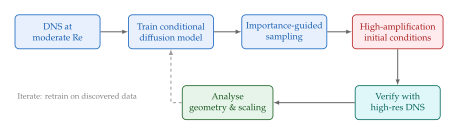
Key Idea.
From Exercises to Research The trajectory from pen-and-paper exercises through coding projects to challenge problems mirrors the path from student to researcher. The exercises build fluency with the mathematical language; the projects develop practical skills with modern frameworks and datasets; and the challenges require the creative synthesis of ideas that defines original scientific work. We encourage every reader to attempt at least one challenge problem-even a partial attempt that fails instructively is worth more than a polished reproduction.
Notes
- We assume well-posedness-existence, uniqueness, and continuous dependence on data-as guaranteed by the Lax–Milgram theorem, the Banach fixed-point theorem, or other classical PDE theory, depending on the equation class.