33 Generative Models for Structured Data
Introduction and Motivation
Consider the following thought experiment. You are a hospital administrator in charge of a research programme on diabetic retinopathy. Your institution holds thousands of patient records: ages, blood glucose levels, comorbidity codes, imaging results, treatment histories, and outcomes. A team of machine learning researchers asks you for access to these records. They want to train a classifier that predicts which patients are at highest risk of vision loss. The model could save sight. The data could save lives.
You say no.
The reasons are familiar to anyone who has worked with sensitive data. Patient privacy regulations (HIPAA in the United States, GDPR in Europe) impose strict limits on data sharing [36]. De-identification is fragile: even removing names and social security numbers leaves quasi-identifiers (age, zip code, admission date) that can be linked to external datasets to re-identify individuals [37]. Institutional review boards move slowly. Data use agreements are labyrinthine. And underneath all the bureaucracy lies a genuine moral concern: these are real people, with real vulnerabilities, and sharing their data, however noble the purpose, carries real risk.
Now imagine a different scenario. Instead of sharing the raw patient records, you share synthetic records: a new dataset, generated by a machine learning model, that preserves the statistical properties of the original data (the correlations, the distributions, the predictive signal) without corresponding to any real individual. The researchers train their classifier on this synthetic dataset and achieve performance comparable to what they would have obtained with the real data. No patient was exposed. No regulation was violated. The model still saves sight.
This is the promise of generative models for structured data, and it is the subject of this chapter. But the promise, as we shall see, is far easier to state than to fulfil.
Key Idea.
The central motivation for structured data generation is the access problem: real-world structured data (patient records, financial transactions, census surveys) is locked behind privacy barriers, licensing restrictions, and institutional politics. Synthetic data, if generated well, can unlock access while preserving utility and protecting privacy.
The Access Problem in Practice
The hospital scenario is not hypothetical. Variants of this dilemma play out daily across industries:
Example 1.
Financial fraud detection. A fintech startup wants to build a fraud detection model, but has only 10,000 transactions in its own database (of which only 12 are confirmed frauds). It cannot access the transaction data of established banks, which collectively hold billions of records with millions of fraud labels. If those banks could share synthetic transaction data, preserving the statistical signatures of fraud while protecting customer identities, the startup could train a far better model. The synthetic data would need to preserve:
The temporal patterns of fraudulent transactions (e.g., multiple small purchases followed by one large purchase).
The geographic correlations (e.g., a card used in New York and then in Lagos within an hour).
The distributional properties of transaction amounts (heavy-tailed, with spikes at round numbers).
The extreme class imbalance (fraud is roughly 0.1% of all transactions).
Example 2.
Educational data. Researchers studying achievement gaps need student-level data linking test scores, demographic variables, school characteristics, and socioeconomic indicators. Such data exists in abundance within school districts, but sharing it would violate FERPA (the Family Educational Rights and Privacy Act). Synthetic educational records, if they preserve the correlations between demographics and outcomes, could enable research that is currently impossible without lengthy data use agreements.
Beyond Images and Text
The past decade has witnessed a revolution in generative modelling. Generative adversarial networks (GANs) produce photorealistic faces [38]. Diffusion models generate artwork that wins competitions [24]. Large language models write poetry, code, and legal briefs [39]. These achievements are genuinely impressive. They are also, from the perspective of data types, remarkably narrow.
Images are regular grids of pixels. Each pixel is a tuple of continuous intensity values (red, green, blue) arranged in a fixed two-dimensional spatial layout. The data type is homogeneous: every element is a real number in . The spatial structure is regular: every pixel has the same neighbourhood geometry. Text is a sequence of tokens drawn from a fixed vocabulary. The data type is again homogeneous: every element is a discrete symbol from a known alphabet. The sequential structure is regular: one token follows another, left to right.
Structured data is neither of these things.
Example 3.
Consider a row from the US Census Bureau's American Community Survey. A single record might contain:
Age: a continuous variable (e.g., 34.5 years).
Income: a continuous variable with heavy right skew and exact zeros (e.g., $0, $23,400, $1,250,000).
Education: an ordinal categorical variable with 16 levels (“No schooling”, “Nursery school”, , “Doctorate”).
Occupation: a nominal categorical variable with over 500 codes.
State: a nominal categorical variable with 51 levels (50 states plus DC).
Marital status: a nominal categorical variable with 5 levels.
Hours worked per week: a discrete variable (0, 1, 2, , 99) with spikes at 0, 20, 35, and 40.
Health insurance: a binary variable (yes/no).
A single row thus contains continuous, discrete, ordinal, nominal, and binary features, all entangled in complex correlations. Generating realistic synthetic census records requires getting all of these right simultaneously.
The fundamental difficulty is that structured data combines heterogeneous types in complex, constraint-laden relationships. There is no spatial grid, no fixed vocabulary, no universal tokenization. Each column lives in its own space, with its own distribution, its own semantics, and its own quirks. And the columns are not independent: income correlates with education, hours worked correlates with occupation, and all of them correlate with age in ways that are subtle, nonlinear, and often domain-specific.
Insight.
The core challenge of structured data generation can be stated in a single sentence: unlike images and text, structured data has no universal inductive bias. Images have spatial locality (nearby pixels are correlated), exploited by convolutions. Text has sequential dependency (the next word depends on preceding words), exploited by attention. Structured data has no such universal structure, and therefore requires fundamentally different generative strategies.
Why Structured Data Matters
If structured data is so difficult, why bother? The answer is that structured data is, by a wide margin, the most common form of data in the world. Estimates vary, but enterprise data warehouses, government databases, financial systems, and healthcare records collectively contain orders of magnitude more structured data than the entire corpus of images or text on the internet. When a business analyst queries a database, when a clinician reviews a patient chart, when a regulator audits a bank, they are working with structured data.
The applications of synthetic structured data are vast:
Privacy-preserving data sharing. As in our hospital example, synthetic data enables sharing across institutional boundaries without exposing individuals. This is critical in healthcare, finance, and government, where privacy regulations are strictest.
Data augmentation for rare events. Fraud detection models struggle because fraudulent transactions are rare (often less than 0.1% of all transactions). Generating synthetic fraud cases can balance the training set and improve classifier performance.
Software testing and development. Software teams need realistic test data to validate database schemas, query performance, and application logic. Synthetic data provides this without copying production databases into development environments.
Fairness auditing. To audit a model for bias, one needs to test it on populations that may be underrepresented in the training data. Synthetic data can fill these gaps, enabling counterfactual fairness analyses.
Simulation and planning. Urban planners, epidemiologists, and supply chain managers all need realistic synthetic populations to run simulations. The US Census Bureau itself produces synthetic data [1] for precisely this purpose.
Education and reproducible research. Researchers who cannot share their original data can share synthetic versions, enabling others to reproduce analyses and verify results.
Historical Note.
The idea of using synthetic data as a privacy-preserving proxy dates back at least to the work of Donald Rubin in 1993 [1], who proposed “multiple synthetic datasets” as a mechanism for protecting confidentiality in public-use microdata. The Census Bureau adopted variants of this approach for the Longitudinal Business Database and other products. What has changed in the past decade is not the idea but the technology: deep generative models can now capture far more complex distributions than the parametric models Rubin envisioned.
A Roadmap for this Chapter
This chapter traces the arc of structured data generation from its earliest challenges to its most recent breakthroughs. We begin here, in Introduction and Motivation, with motivation and context. In The Landscape of Structured Data, we survey the landscape of structured data types. In Challenges in Structured Data Generation, we catalogue the fundamental challenges that make structured data generation hard. Subsequent sections then address each challenge in turn, presenting the key models and methods:
CTGAN (CTGAN – The Foundation): the conditional tabular GAN that introduced mode-specific normalisation and training-by-sampling.
CTAB-GAN+ (CTAB-GAN+ – The Next Generation): the next-generation tabular GAN with auxiliary classifiers and enhanced privacy.
TabDDPM (TabDDPM – Diffusion Models for Tabular Data): diffusion models adapted for mixed-type tabular data.
GOGGLE (GOGGLE – Graph-Optimized Generation): graph-based generation that explicitly models relational structure.
LLM-based approaches: TabuLa, Tabby, and DeLTa, which leverage large language models for tabular generation.
Harpoon (Harpoon – Manifold-Guided Diffusion for Tabular Data): a recent method addressing multi-table relational data.
Along the way, we will encounter deep connections to differential privacy, optimal transport, score matching, and graph neural networks. By the end of this chapter, you will have a comprehensive understanding of why structured data generation is hard, what the current best solutions are, and where the open problems lie.

The Landscape of Structured Data
Before we can generate structured data, we must understand what it is. The term “structured data” is used loosely in the literature; different communities mean different things by it. In this chapter, we adopt a broad definition that encompasses the major forms of non-image, non-text data encountered in machine learning practice.
Definition 1 (Structured Data).
Structured data is data organised according to a predefined schema that specifies the names, types, and relationships of its constituent elements. Unlike unstructured data (images, audio, free text), structured data has an explicit schema that constrains the values each element can take and the relationships between elements.
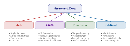
This definition is deliberately broad. It includes tabular data (the most common form), graph-structured data, time series, and relational databases. Each of these presents its own generative challenges, and each has spawned its own family of methods. Let us survey them in turn.
Tabular Data
Tabular data is the bread and butter of data science. It is the format of spreadsheets, SQL databases, CSV files, and Pandas DataFrames. A tabular dataset consists of rows (records, observations, samples) and columns (features, attributes, variables), arranged in a matrix-like structure where each row represents an independent entity and each column represents a measured property.
Definition 2 (Tabular Data).
A tabular dataset is a collection where each row is a -dimensional vector. The columns are partitioned into types: (CONT) such that . We assume the rows are drawn i.i.d. from an unknown joint distribution .
The i.i.d. assumption is a simplification; real tabular data sometimes exhibits temporal drift or hierarchical structure. But it is the standard assumption in the tabular generation literature, and it is where most methods begin.
Column types in the wild.
The clean partition into continuous, categorical, and ordinal columns masks considerable practical complexity. Real-world columns exhibit a rich variety of quirks:
Multimodal continuous columns. Income is not Gaussian: it has a spike at zero (for unemployed or retired individuals), a broad mode around the median, and a heavy right tail. Age has spikes at round numbers (people report “30” more often than “31”).
High-cardinality categorical columns. ZIP codes in the US have over 40,000 unique values. ICD-10 medical diagnosis codes have over 70,000. Standard one-hot encoding becomes impractical at this scale.
Mixed-type columns. A “dose” column might be “None” (categorical), “Low”, “Medium”, “High” (ordinal), or a precise numerical value like 2.5 mg (continuous). How should a generative model represent this?
Missing values. Real tabular data is riddled with missing values, often with non-random missingness patterns. A “missing” income might mean unemployment, refusal to report, or data entry error, each with different statistical properties.
Implicit constraints. If a patient's “pregnant” column is “yes”, their “sex” column must be “female”. If “employment status” is “retired”, “age” is unlikely to be 25. These logical and statistical constraints are nowhere in the schema but everywhere in the data.
Definition 3 (Column Types).
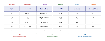
Given a tabular dataset with columns, we define the following column type taxonomy:
Continuous: . The column admits a probability density function. Examples: age, temperature, stock price.
Nominal categorical: with no natural ordering. Examples: country, diagnosis code, colour.
Ordinal categorical: with a total ordering. Examples: education level, severity grade, satisfaction rating.
Binary: . A special case of nominal categorical with .
Discrete numerical: (or a subset thereof). Unlike categorical columns, arithmetic operations are meaningful. Examples: number of children, hospital length of stay.
Exercise 1.
For each of the following columns, determine the column type and explain any ambiguities:
Customer age (recorded as integer years).
Credit score (FICO, range 300–850).
Blood type (A, B, AB, O, with +/– Rh factor).
Temperature in Celsius.
Star rating of a restaurant (1–5 stars).
Number of prior convictions (0, 1, 2, ).
Hint: Several of these admit multiple valid classifications. The “right” choice depends on the downstream generative model.
Remark 1.
The distinction between column types is not always clear-cut, and reasonable people may disagree. Consider credit scores: they are technically discrete (only integer values between 300 and 850 are possible), but the range is large enough that treating them as continuous is often sensible. Conversely, a “number of bedrooms” column takes values in : the range is small enough that treating it as categorical might work better than treating it as continuous. The “right” column type for a generative model depends on the model architecture, the downstream task, and the distribution of the data. We will see this theme recur throughout the chapter.
The geometry of tabular data.
It is instructive to think about what tabular data looks like geometrically. Each row is a point in the product space . For a table with three continuous columns, this is simply , and we can visualise the data as a point cloud. But for a table with a mix of continuous and categorical columns, the space is more exotic. Consider a table with one continuous column (income) and one categorical column (state, with 51 values). The data space is , which can be visualised as 51 parallel real lines. The data forms clusters on these lines, and the distribution on each line may be very different (income distributions vary dramatically across states). A generative model must capture both the within-line distributions and the relative densities across lines.
For a table with continuous columns and categorical columns (with cardinalities ), the data space is . This is a disjoint union of copies of , one for each combination of categorical values. The number of copies grows exponentially with the number of categorical columns, which is why high-dimensional tabular generation is so challenging: the model must learn a separate continuous distribution for each categorical combination, but most combinations are rarely (or never) observed.
Exercise 2.
Consider a tabular dataset with two continuous columns () and one binary column ().
Describe the data space geometrically.
Suppose the conditional distributions and are both bivariate Gaussians with different means and covariances. How many parameters fully characterise ?
Now add a second categorical column . How does the number of parameters scale?
Explain why this exponential scaling motivates the use of neural network-based generative models.
Graph-Structured Data
Not all structured data fits neatly into rows and columns. Consider a social network: each person is a node with attributes (age, location, interests), and friendships are edges with their own attributes (since when, interaction frequency). A molecular graph represents atoms as nodes and chemical bonds as edges. A knowledge graph represents entities and their relationships. In each case, the topology of the graph (which nodes are connected to which) is itself part of the data that must be generated.
Formally, a graph consists of a node set , an edge set , node feature matrices , and edge feature matrices . Generating a realistic graph thus requires simultaneously generating the topology and the attributes . This is harder than tabular generation for at least two reasons:
Variable size. The number of nodes and edges varies across graphs. A generative model must decide how large each generated graph should be.
Permutation invariance. The same graph can be represented by different adjacency matrices (by permuting node labels). A generative model should ideally be invariant to this relabelling.
Graph generation connects deeply to the molecular design literature (where generating valid drug candidates is the goal), the social network literature (where realistic synthetic networks are needed for simulation), and the combinatorial optimisation literature (where graph generation is a form of constructive heuristic) [7].
Time Series Data
A time series is a sequence of observations indexed by time: , where each is a -dimensional measurement at time . Unlike tabular data, where rows are (assumed) independent, time series observations are temporally dependent: the value at time depends on preceding values. This temporal structure is the defining characteristic and the principal generative challenge.
Autocorrelation. A realistic synthetic stock price must exhibit the same autocorrelation structure as real prices: volatility clustering, mean reversion, and fat-tailed returns.
Irregular sampling. Medical time series (vital signs, lab tests) are recorded at irregular intervals. The sampling pattern itself carries information (a patient monitored every hour is sicker than one monitored daily).
Non-stationarity. Many real-world time series (economic indicators, climate data) have statistical properties that change over time. A generative model must capture these drifts.
Time series generation is related to, but distinct from, time series forecasting. Forecasting extends an observed prefix; generation creates entire sequences from scratch. The methods overlap (both use recurrent networks, transformers, and diffusion models) but the evaluation criteria differ.
Example 4.
An electrocardiogram (ECG) is a multivariate time series with 12 leads, each sampled at 250–500 Hz for 10 seconds. A cardiologist can diagnose arrhythmias, myocardial infarction, and other conditions from the morphology of the waveform. Generating realistic synthetic ECGs requires preserving the precise morphological features (P-wave, QRS complex, T-wave), the inter-lead correlations (lead II should be approximately the sum of leads I and III), and the patient-level variability (normal heart rates range from 60 to 100 beats per minute, with considerable variation in waveform shape). A generative model that produces ECGs with the right frequency spectrum but the wrong morphology would fool a statistical test but not a cardiologist.
Exercise 3.
Propose three evaluation metrics for synthetic time series data that capture different aspects of quality:
A metric that measures the fidelity of the marginal distribution at each time step.
A metric that measures the fidelity of the temporal autocorrelation structure.
A metric that measures downstream predictive utility (train-on-synthetic, test-on-real).
For each metric, describe how it would be computed, what pathological failure modes it would detect, and what failure modes it would miss.
Relational Data
Perhaps the most challenging form of structured data is
relational data: multiple tables connected by foreign key
relationships, as in a relational database. Consider an e-commerce
database with tables for customers, orders,
products, and order_items. A single customer has
zero or more orders, each order has one or more items, and each item
references a product. Generating synthetic relational data requires
not only generating realistic rows in each table but also preserving
the referential integrity (every foreign key points to a
valid primary key) and the cross-table correlations (a
customer's demographics should be consistent with their purchasing
patterns).
Remark 2.
The relational data generation problem is strictly harder than tabular generation: a single-table dataset is a relational database with one table and no foreign keys. Most methods in the literature focus on the single-table case; extending them to multi-table settings is an active research frontier [2].
Exercise 4.
Classify each of the following datasets as tabular, graph, time series, relational, or a combination. Justify your answer.
A hospital database with tables for patients, visits, diagnoses, and medications.
A CSV file of Airbnb listings with price, neighbourhood, number of reviews, and host information.
A social network with user profiles and friendship edges.
A collection of electrocardiogram (ECG) recordings, each consisting of 12 leads sampled at 500 Hz for 10 seconds.
A knowledge graph of biomedical entities (genes, diseases, drugs) and their relationships.
A single table of credit card transactions with timestamp, amount, merchant, and fraud label.
Hint: Some datasets admit multiple valid classifications; the most useful classification depends on the generative task.
Challenges in Structured Data Generation
Having surveyed the landscape, we now turn to the heart of the matter: why is generating structured data so hard? The difficulties are numerous, interconnected, and often domain-specific. In this section, we organise them into a taxonomy of challenges. Each challenge will be addressed by one or more of the methods we present in subsequent sections; our goal here is to lay out the full scope of the problem before reaching for solutions.
The Mixed-Type Challenge
The most fundamental challenge in tabular data generation is that columns have different types, and no single representation works well for all of them.
Consider a generator based on a neural network. The network produces a vector of real numbers as output. How should we interpret this output? For a continuous column like “income”, the output can be used directly (after appropriate denormalisation). For a categorical column like “state” (with 51 categories), we need to convert a real-valued vector into a discrete choice. For a binary column like “insured”, we need a probability and a threshold. For a discrete numerical column like “hours worked per week” (with spikes at 0, 20, 35, and 40), we need something that is neither purely continuous nor purely categorical.
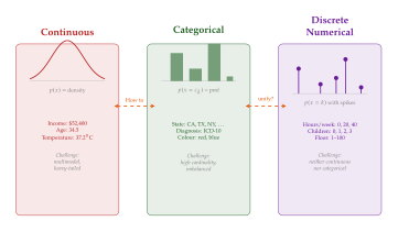
The mathematical crux of the problem is that the joint distribution lives in a product space: (Product Space) where for continuous columns, for categorical columns, and so on. This product space is neither continuous (because of the categorical dimensions) nor discrete (because of the continuous dimensions). It is a hybrid space, and probability distributions over hybrid spaces do not have a single natural parameterisation.
Caution.
A common but incorrect approach is to “just treat everything as continuous”: encode categorical columns as integers (e.g., “California” 1, “Texas” 2) and feed the result into a standard continuous generator (e.g., a GAN or VAE). This fails spectacularly. The model generates fractional categories (e.g., state = 1.37), imposes a spurious ordering (California Texas New York), and collapses rare categories. Equally, treating everything as categorical by discretising continuous columns into bins loses fine-grained distributional information.
The key insight, which we will formalise when we study CTGAN in CTGAN – The Foundation, is that each column type requires its own representation and its own loss function:
Continuous columns mode-specific normalisation mean squared error.
Categorical columns one-hot encoding cross-entropy loss.
Discrete numerical columns hybrid strategies that combine aspects of both.
The Correlation Challenge
Even if we solve the mixed-type problem for each column individually, we face a deeper challenge: the columns are not independent. The joint distribution is not the product of its marginals . The correlations between columns carry the information that makes data useful, and destroying them renders the synthetic data worthless.
Example 5.
In a medical dataset, the following correlations are essential:
Age and blood pressure are positively correlated (blood pressure tends to increase with age).
Diagnosis and medication are strongly correlated (patients with diabetes are prescribed insulin, not antibiotics).
Gender and pregnancy status have a deterministic relationship (only female patients can be pregnant).
Income and insurance type are correlated in complex, nonlinear ways (low-income patients may have Medicaid, while high-income patients may have private insurance, but the relationship varies by state).
A synthetic medical dataset that fails to reproduce these correlations would be useless for training clinical prediction models, testing decision support systems, or evaluating treatment protocols.
The correlation structure of a tabular dataset can be conceptualised at multiple levels:
Pairwise (marginal) correlations. The correlation between any two columns. Pearson's for continuous–continuous pairs, Cramér's for categorical–categorical pairs, and various mixed measures for continuous–categorical pairs.
Conditional correlations. The correlation between two columns given a third. For instance, the correlation between income and education may differ across age groups.
Higher-order interactions. Patterns that involve three or more columns simultaneously. For example, the combination (male, age , smoker) may have a specific risk profile that is not captured by any pairwise relationship.
Functional dependencies. Deterministic relationships between columns. Zip code determines city and state. BMI is exactly weight/(height). These are not statistical correlations but logical constraints.
Definition 4 (Correlation Structure).
The correlation structure of a tabular dataset is the collection of all statistical dependencies among its columns, formally characterised by the joint distribution . We say that a synthetic dataset preserves the correlation structure of if the joint distributions are “close” under an appropriate divergence: (Correlation Preservation) where is a statistical divergence (e.g., KL divergence, total variation, maximum mean discrepancy) and is a tolerance.
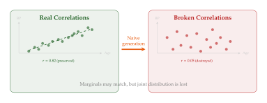
A particularly insidious failure mode is what we might call the “marginal trap”. A generative model produces synthetic data where each column, viewed in isolation, looks realistic: the distribution of ages matches, the distribution of incomes matches, the distribution of states matches. But the joint distribution is wrong: the correlations between columns have been destroyed. The synthetic data passes marginal tests with flying colours but fails joint tests miserably.
Key Idea.
Marginal fidelity is necessary but not sufficient. A synthetic dataset must reproduce not only the marginal distributions of individual columns but also the full correlation structure. Evaluating only marginals gives a dangerously optimistic picture of synthetic data quality.
The difficulty of preserving correlations grows rapidly with the dimensionality of the data. For a table with columns, there are pairwise correlations, three-way interactions, and so on. Capturing all of these with finite data and finite model capacity is a fundamentally hard problem, closely related to the curse of dimensionality in density estimation.
Proposition 1 (Exponential Growth of Interaction Terms).
For a tabular dataset with columns, the number of -way interaction terms is . The total number of interactions up to order is: (Interactions) For columns and (up to three-way interactions), this gives interaction terms. Capturing all pairwise and three-way interactions in a 50-column table is a substantial statistical challenge.
In practice, most methods rely on the neural network's capacity to implicitly learn the relevant correlations from data, rather than explicitly modelling each interaction. Whether this implicit approach suffices, or whether explicit correlation modelling (as in GOGGLE's graph-based approach [7]) is necessary, remains an active debate.
Exercise 5.
Given a real dataset and a synthetic dataset , both with the same schema, describe a hypothesis testing procedure to determine whether preserves the pairwise correlation structure of . Your procedure should:
Handle continuous–continuous, continuous–categorical, and categorical–categorical column pairs.
Account for multiple testing (you are comparing pairs).
Produce a single summary statistic and a -value.
Hint: Consider using Cramér's for categorical pairs, Pearson's for continuous pairs, and the correlation ratio for mixed pairs, combined with a Bonferroni or Benjamini–Hochberg correction.
The Constraint Satisfaction Challenge
Beyond statistical correlations, real-world structured data satisfies a host of hard constraints: logical, physical, regulatory, and domain-specific. Violating these constraints produces synthetic records that are not merely statistically implausible but logically impossible.
Example 6.
The following constraints are common in healthcare data:
Logical: if “pregnant” = yes, then “sex” = female.
Range: blood oxygen saturation %.
Functional: BMI .
Temporal: discharge date admission date.
Referential: every prescription must reference a valid patient ID.
Domain: a deceased patient cannot have follow-up visits.
A standard GAN has no mechanism to enforce any of these constraints. It may generate a pregnant 85-year-old male with an SpO of % who was discharged before being admitted.
Constraints can be categorised along two axes:
Hard vs. soft. Hard constraints must be satisfied exactly (e.g., SpO). Soft constraints are statistical regularities that should be approximately respected (e.g., most people over 65 are retired).
Explicit vs. implicit. Explicit constraints are documented in the schema or domain knowledge. Implicit constraints are discovered only by inspecting the data (e.g., no one in the dataset has both income and education “No schooling”, but this is not a logical impossibility).
Handling constraints in generative models is an active area of research. Current approaches fall into three categories:
Post-hoc rejection/correction. Generate unconstrained samples and either reject those that violate constraints or correct them. Simple but wasteful, and correction can distort the learned distribution.
Architectural enforcement. Design the generator architecture so that constraint violations are impossible (e.g., using softmax to ensure probabilities sum to 1, or clipping outputs to valid ranges). Effective for simple constraints but brittle for complex ones.
Loss-based guidance. Add penalty terms to the generator's loss function that discourage constraint violations. Flexible but does not guarantee satisfaction.
Exercise 6.
Design a post-processing pipeline that enforces the following constraints on synthetic healthcare records:
.
If pregnant yes, then sex female.
BMI weight/height (to within rounding error).
Discharge date admission date.
For each constraint, describe: (a) how to detect a violation, (b) how to correct it, and (c) what distributional distortion the correction might introduce.
The Evaluation Challenge
Suppose you have generated a synthetic dataset. How do you know it is “good”? For images, the answer is relatively well established: Fréchet Inception Distance (FID) measures distributional similarity using features from a pre-trained network [40]. For text, perplexity and human evaluation provide useful signals. For structured data, the evaluation landscape is far more fragmented, and there is no single universally accepted metric.
Definition 5 (Synthetic Data Fidelity).
The fidelity of a synthetic dataset with respect to a real dataset is a measure of how closely the statistical properties of match those of . Fidelity can be assessed at multiple granularities:
Marginal fidelity: the marginal distribution of each column in matches that in .
Pairwise fidelity: the pairwise joint distributions match.
Full distributional fidelity: the full joint distribution is close to under an appropriate divergence.
Fidelity is necessary, but it is only one dimension of quality. A comprehensive evaluation considers multiple axes:
Axis 1: Statistical fidelity.
Does the synthetic data have the same distributions, correlations, and higher-order statistics as the real data? Common metrics include:
Column-wise distributional tests (Kolmogorov–Smirnov for continuous, chi-squared for categorical).
Pairwise correlation matrices (Pearson's , Cramér's ).
Maximum mean discrepancy (MMD) between real and synthetic feature distributions.
Axis 2: Machine learning utility.
Can a model trained on synthetic data perform comparably to one trained on real data? The standard protocol is “train on synthetic, test on real” (TSTR): train a classifier or regressor on , evaluate on a held-out portion of , and compare against a model trained on itself [4].
Axis 3: Privacy.
Does the synthetic data protect the privacy of individuals in the training set? Key metrics include:
Distance to closest record (DCR): the minimum distance from each synthetic record to the nearest real record.
Membership inference attack accuracy: can an adversary determine whether a specific individual was in the training data?
Attribute inference risk: given partial knowledge of a record, can an adversary infer sensitive attributes?
Axis 4: Diversity.
Does the synthetic data exhibit the full diversity of the real data, or has the generator collapsed to a subset of modes? This is related to the mode collapse problem in GANs, and is measured by coverage metrics and support size estimates.
Axis 5: Constraint satisfaction.
Does the synthetic data satisfy known domain constraints? This axis is specific to structured data and is absent in the image generation literature.
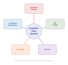
Remark 3.
The evaluation challenge is not merely a practical inconvenience; it reflects a deeper conceptual issue. What does it mean for synthetic data to be “good”? Perfect fidelity (the synthetic distribution exactly matches the real distribution) is both unreachable and, paradoxically, undesirable: if the synthetic data is a perfect copy of the real data, it provides no privacy protection. The goal is not fidelity but utility: the synthetic data should be useful for its intended purpose, whatever that purpose may be. Different purposes require different evaluation criteria.
The Privacy–Utility Tradeoff
The most fundamental tension in synthetic data generation is between privacy and utility. These two goals are inherently at odds: the more faithfully the synthetic data reproduces the real data, the more information it leaks about the individuals in the real data. Conversely, the more aggressively we protect privacy, the more we degrade the statistical properties that make the data useful.
This tradeoff is formalised by differential privacy [41], which provides a mathematically rigorous framework for quantifying privacy loss.
Definition 6 (Privacy Guarantee).
A randomised mechanism satisfies -differential privacy if for all datasets differing in at most one record, and for all measurable subsets : (DP) The parameter is the privacy budget: smaller means stronger privacy. The parameter allows a small probability of failure.
The key implication for synthetic data is this: if we train a generative model on real data using a differentially private optimiser (e.g., DP-SGD [17]), then the trained model is itself differentially private, and any synthetic data sampled from inherits the privacy guarantee (by the post-processing theorem of differential privacy).
The tradeoff manifests as follows:
Low (strong privacy). Noise added during training is large. The model learns a blurred version of the real distribution. Synthetic data has poor fidelity and low ML utility.
High (weak privacy). Noise is small. The model learns the real distribution accurately. Synthetic data has high fidelity and high ML utility, but the privacy guarantee is weak.
Intermediate . The practical sweet spot, where the synthetic data is “good enough” for the intended purpose while providing “strong enough” privacy for the regulatory context.
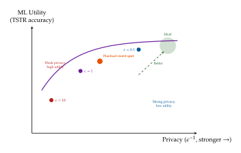
Insight.
The privacy–utility tradeoff is not a failure of current methods; it is a fundamental limitation. Information theory tells us that a mechanism providing -differential privacy can transmit at most nats of information about any individual. The question is not whether the tradeoff exists but where the frontier lies and how to push it outward. Every method in this chapter can be viewed as an attempt to improve the privacy–utility Pareto frontier.
The Scalability Challenge
Production tabular datasets can be large along multiple dimensions: millions of rows, hundreds or thousands of columns, and complex schemas with dozens of tables. Scalability challenges arise in several forms:
Column-count scalability. One-hot encoding a categorical column with categories adds dimensions. A table with 50 categorical columns averaging 100 categories each becomes a 5,000-dimensional one-hot vector. Training a GAN in 5,000 dimensions is non-trivial.
Row-count scalability. Training generative models on millions of rows is computationally expensive, particularly for diffusion models that require multiple denoising steps per sample.
Schema complexity. Multi-table datasets with complex foreign key relationships require models that scale with the number of tables and the depth of the join graph.
Conditional generation. Generating data conditioned on specific constraints (e.g., “generate 1,000 records of female patients over 65 with diabetes”) requires the model to navigate high-dimensional conditional distributions efficiently.
The Temporal Challenge
When tabular data has a temporal dimension (e.g., financial transactions with timestamps, patient visits over time), the i.i.d. assumption breaks down. Rows are no longer exchangeable: their order matters, and the dependencies between them carry crucial information.
A sequence of credit card transactions for a single customer exhibits patterns (regular purchases at a grocery store every Tuesday, a rent payment on the first of each month) that a generative model must capture. Merely generating i.i.d. transactions with the right marginal distributions would produce a customer whose spending pattern is random noise.
The temporal challenge connects structured data generation to the broader field of time series generation, but with the additional complication that each “time step” is a mixed-type tabular record, not a simple numerical vector.
A Unified View of the Challenges
Let us step back and view the challenges holistically. At the highest level of abstraction, generating structured data requires learning a joint distribution over a product of heterogeneous spaces, subject to hard constraints, with limited data, while providing privacy guarantees and preserving the correlations that make the data useful. Each challenge corresponds to an aspect of this problem that is trivial for images or text but difficult for structured data:
| Challenge | Images | Structured Data |
| Data type | Homogeneous (pixels) | Heterogeneous (mixed) |
| Structure | Regular grid | No universal structure |
| Correlations | Spatial locality | Arbitrary pairwise |
| Constraints | Few (pixel range) | Many (domain-specific) |
| Evaluation | FID, IS | No standard metric |
| Privacy | Less critical | Often required |
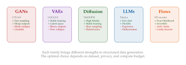
Exercise 7.
For each of the following application scenarios, rank the five generative model families (GAN, VAE, Diffusion, LLM, Flow) from most to least suitable. Justify your ranking.
A hospital needs to generate 10 million synthetic patient records with -differential privacy for sharing with an external research consortium.
A startup with only 200 labelled examples needs to generate augmentation data for a fraud detection model.
A government agency needs to generate a synthetic census with 300 columns and 50 million rows, with exact constraint satisfaction (e.g., household relationships must be consistent).
A pharmaceutical company needs to generate realistic molecular graphs for drug discovery.
The Historical Arc
The field of structured data generation has evolved rapidly. In the span of about a decade, it has progressed from simple Bayesian networks and copula models to sophisticated deep generative architectures that rival or exceed classical methods on standard benchmarks. Understanding this trajectory helps situate the methods we will study.

The historical arc reveals several important trends:
From general-purpose to specialised. Early attempts simply applied standard GANs to tabular data. Success came from specialising the architecture to respect the structure of the data: mode-specific normalisation for multimodal continuous columns, training-by-sampling for imbalanced categories, and hybrid noise processes for mixed-type columns.
From GANs to diversity. The GAN framework dominated tabular generation from 2019 to 2022, but the post-2022 era has seen a rapid diversification: diffusion models (TabDDPM), graph-based methods (GOGGLE), LLM-based approaches (TabuLa, GReaT, Tabby), and multi-table methods (Harpoon). This suggests that no single framework will dominate.
From generation to evaluation. Early papers focused on generating data and reported limited metrics. Recent work increasingly focuses on rigorous evaluation, with standardised benchmarks, multiple metrics, and privacy–utility analyses becoming the norm.
From single-table to multi-table. The field has gradually moved from single flat tables to the richer setting of relational databases. This mirrors the shift in the broader ML community from simple to complex data structures.
Historical Note.
The earliest work on synthetic data generation predates deep learning entirely. The Census Bureau's Synthetic Longitudinal Business Database (SynLBD), released in 2011, used multiple imputation techniques based on sequential regression [1]. Bayesian network methods [3] offered another classical approach, modelling the joint distribution as a directed acyclic graph of conditional distributions. These methods worked well for small, low-dimensional datasets but struggled with the scale and complexity of modern data, motivating the turn to deep generative models.
Formalising the Goal
Having catalogued the challenges, let us formalise what we are trying to achieve. The structured data generation problem can be stated as follows.
Definition 7 (Structured Data Generation Problem).
Given a real dataset drawn i.i.d. from an unknown distribution over a product space , the structured data generation problem is to learn a generative model such that:
Fidelity. Samples are distributed approximately according to : (Fidelity GOAL) for some divergence and tolerance .
Privacy. The training procedure satisfies -differential privacy.
Constraint satisfaction. For a set of constraints , we have for all and all generated samples .
Scalability. The computational cost of training and sampling scales gracefully with (number of rows), (number of columns), and the complexity of .
This formalisation makes explicit what we want and reveals the fundamental tension: requirements 1 and 2 are inherently at odds (the privacy–utility tradeoff), while requirements 1 and 3 may conflict if the learned distribution assigns mass to constraint-violating regions. The art of structured data generation lies in navigating these tensions, and the methods in the following sections represent different strategies for doing so.
What Lies Ahead
With the challenges laid out, we are ready to confront them. The structure of our attack follows the historical arc of the field. We begin with the breakthrough that made tabular data generation practical: CTGAN and its solution to the mixed-type and mode collapse problems. We then study the refinements of CTAB-GAN+, the diffusion-based approach of TabDDPM, the graph-based perspective of GOGGLE, and the LLM-based methods that leverage the power of foundation models. Finally, we address the frontier of multi-table relational generation with Harpoon.
At each stage, we will return to the challenges catalogued in this section and ask: which challenges does this method solve, which does it mitigate, and which does it leave open? By the end of the chapter, you will have not only a toolkit of methods but also a deep understanding of why each method works, where it succeeds, and where it fails.
Exercise 8.
For each of the challenges listed in this section (mixed types, correlations, constraints, evaluation, privacy, scalability, temporal), identify which of the following methods you expect to address it, and explain your reasoning:
You may use information from the brief descriptions in A Roadmap for this Chapter and any prior knowledge of these methods. We will revisit your answers at the end of the chapter.
Exercise 9.
The Fréchet Inception Distance (FID) is the standard evaluation metric for generative image models. Explain why FID cannot be directly applied to tabular data. Then propose a tabular analogue of FID: what feature extractor would you use in place of Inception, and what distributional comparison would you perform? Discuss the limitations of your proposal.
Exercise 10.
Prove that if a generative model is trained using an -differentially private algorithm, then any synthetic dataset sampled from also satisfies -differential privacy. Hint: Use the post-processing theorem of differential privacy: if is -DP and is any (possibly randomised) function, then is also -DP.
Exercise 11.
Consider a tabular dataset with columns (age, continuous), (pregnant, binary), (sex, categorical: M/F), and (number of children, discrete). Write down all the constraints you can identify (both hard and soft). For each constraint, classify it as logical, statistical, range, or functional. Then describe how you would enforce each constraint in a post-processing step without distorting the learned distribution.
Challenge 1.
Open Problem: Universal Structured Data Metric. Design a single metric for synthetic tabular data quality that captures fidelity, utility, privacy, diversity, and constraint satisfaction simultaneously. The metric should be: (a) efficiently computable, (b) interpretable (what does a score of 0.8 mean?), (c) applicable to datasets with arbitrary column types, and (d) validated against human judgments of synthetic data quality. No such metric currently exists.
Challenge 2.
Open Problem: Constraint-Aware Generation. Design a generative model architecture that can accept an arbitrary set of logical constraints (expressed, say, in first-order logic) and guarantee that every generated sample satisfies all constraints, without post-hoc rejection or correction. The model should maintain high fidelity and should not require retraining when the constraint set changes.
CTGAN – The Foundation
Before 2019, the dream of generating realistic tabular data with generative adversarial networks was, to put it politely, a dream deferred. Researchers had tried the obvious approach: take a GAN, feed it rows of tabular data, train, and hope. The results were consistently disappointing. Generated tables exhibited bizarre artefacts – continuous columns collapsed to a single mode, rare categories vanished entirely, and the correlations between columns that make real data useful dissolved into noise. The problem was not that GANs were incapable of modelling structured data; the problem was that nobody had figured out how to speak the language of tabular data in a form that GANs could understand.
The breakthrough came from Lei Xu, Maria Skoularidou, Alfredo Cuesta-Infante, and Kalyan Veeramachaneni at MIT, who published CTGAN – the Conditional Tabular GAN – in 2019 [4]. Their insight was deceptively simple: the failure of previous tabular GANs was not a failure of architecture but a failure of representation. Continuous columns in real data are often multimodal; categorical columns are often imbalanced. Standard GAN training, which assumes that the data distribution is smooth and that all modes are equally important, is catastrophically ill-suited to these realities.
CTGAN introduced three innovations that, together, cracked the code:
Mode-specific normalisation: fitting a variational Gaussian mixture model (VGM) to each continuous column and representing values as (mode indicator, normalised residual) pairs.
Training-by-sampling: a conditional generation strategy that forces the generator to produce samples from every category, including rare ones, thereby combating mode collapse on discrete columns.
PacGAN integration: packing multiple generated samples together before feeding them to the discriminator, providing a structural defence against mode collapse.
Each of these ideas is individually straightforward; their power lies in the combination. In the sections that follow, we dissect each component with full mathematical detail, build up the architecture piece by piece, and prove the key properties that make CTGAN work.
Historical Note.
The name “CTGAN” stands for Conditional Tabular GAN, but the “conditional” refers not to conditional generation in the sense of cGAN [8], but rather to the training-by-sampling strategy that conditions the generator on a randomly selected category at each training step. This naming has caused some confusion in the literature; it is worth noting that CTGAN can generate both conditionally and unconditionally at inference time.
The Architecture
Let us begin with the overall architecture. CTGAN uses a generator–discriminator pair, both fully connected, but with crucial modifications that distinguish it from a vanilla GAN.
Generator.
The generator takes two inputs: a noise vector drawn from a -dimensional standard Gaussian, and a conditional vector that specifies which category (and which column) the generated row should exhibit. The concatenated input passes through a stack of fully connected layers with batch normalisation and ReLU activations: (Layer) where , and are the weight matrix and bias vector of layer . The final layer uses a combination of activation functions matched to the output representation:
Tanh for the normalised continuous values (which lie in after mode-specific normalisation).
Softmax for the mode indicator one-hot vectors of each continuous column.
Gumbel-softmax for the one-hot representations of categorical columns.
Remark 4.
The use of Gumbel-softmax for categorical columns is essential. A standard softmax produces a probability vector, but the discriminator expects a one-hot vector (since real data is one-hot). The Gumbel-softmax trick [9] provides a differentiable approximation to sampling from a categorical distribution, allowing gradients to flow through the discrete choice during training while producing approximately one-hot outputs.
Discriminator.
The discriminator takes a (possibly packed) tabular row and outputs a scalar score. Its architecture is also fully connected but uses leaky ReLU activations and dropout: (Layer) where is the dropout probability (typically ). The use of leaky ReLU rather than ReLU avoids the dying neuron problem, while dropout acts as a regulariser that prevents the discriminator from memorising specific real samples.
Definition 8 (Conditional Generator).
Let denote the set of all categories across all discrete columns of a tabular dataset . A conditional generator is a function that maps a noise vector and a one-hot conditional vector (with ) to a synthetic tabular row , where is the dimensionality of the encoded row representation. The conditional vector specifies that category is active, meaning the generated row must contain category in the corresponding column.
Now we turn to PacGAN, one of CTGAN's most important defences against mode collapse.
Definition 9 (PacGAN Discriminator).
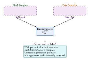
Let be an integer called the packing degree. A PacGAN discriminator is a function that receives a pack of tabular rows concatenated into a single input vector of dimension and produces a scalar score. During training, each pack is formed by drawing independent samples either all from the real data or all from the generator: (REAL) The discriminator must judge whether the entire pack is real or fake, forcing it to evaluate the joint distribution of the pack rather than each sample individually.
Insight.
Why PacGAN works. Consider a generator that has collapsed to producing only one mode of a bimodal distribution. A standard discriminator sees individual samples and may accept each one as plausible – after all, each sample does lie on a real mode. But a PacGAN discriminator sees groups of samples. If the generator only produces one mode, then every pack consists of samples from that single mode. Real packs, by contrast, contain a mix of modes. The discriminator can detect this distributional anomaly and penalise the generator, creating a gradient signal toward diverse generation. Lin et al. [10] proved that for a discriminator with packing degree , any generator equilibrium must have at least modes, providing a structural guarantee against mode collapse.
The following TikZ diagram shows the full CTGAN architecture.
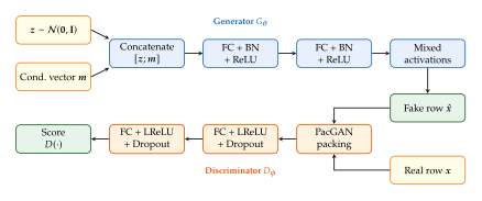
The next diagram illustrates the PacGAN packing concept in detail.
Mode-Specific Normalisation in Detail
We now turn to the heart of CTGAN's preprocessing strategy: mode-specific normalisation (MSN). This technique addresses a fundamental mismatch between the assumptions of neural networks and the reality of tabular continuous columns.
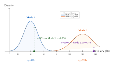
Standard neural network training assumes that input features are roughly Gaussian or at least unimodal. Batch normalisation, weight initialisation schemes, and the geometry of gradient descent all work best when the data is centred and symmetric. But continuous columns in real-world tabular data are often wildly non-Gaussian. A salary column might have one mode around $40,000 for entry-level employees and another around $120,000 for senior staff. An age column might be roughly uniform. A transaction amount column might follow a power law with a massive spike at zero.
If we naively min–max normalise such a column to , we compress the multimodal structure into a range where the generator must learn to reproduce multiple peaks – a task that standard generators handle poorly. Mode-specific normalisation solves this by decomposing each continuous column into a mixture of Gaussians, then representing each value relative to the Gaussian mode it most likely belongs to.
The procedure has three steps.
Step 1: Fit a Variational Gaussian Mixture.
For each continuous column in the dataset, we fit a variational Gaussian mixture model (VGM) with components. Let the fitted parameters be where is the weight, the mean, and the standard deviation of component . The VGM is fitted using variational Bayesian inference, which automatically prunes components with negligible weight, effectively performing model selection.
Remark 5.
The choice of VGM over standard EM-fitted Gaussian mixtures is deliberate. Variational inference places a Dirichlet prior on the mixture weights, which drives unnecessary components to zero weight. This means we can initialise with a generous number of components (e.g., ) and let the algorithm discover the true number of modes. In practice, columns with unimodal distributions end up with a single active component, while multimodal columns retain the appropriate number.
Step 2: Assign Mode and Normalise.
For a value in column , we compute the probability that belongs to each mode: (Assignment) where is the standard normal density. We then sample a mode: (Sample) and compute the normalised value within that mode: (Normalize) The factor of 4 ensures that approximately 99.99% of the values within a given mode fall in the range , which matches the range of the tanh activation in the generator output layer.
Step 3: Encode as (Mode One-Hot, Normalised Value).
The final representation of value in column is the pair where is a one-hot vector with a 1 in position and zeros elsewhere, and is the normalised scalar. The generator must produce both (via softmax) and (via tanh) for each continuous column.
Algorithm 1.
Mode-Specific Normalisation Procedure
Input: Tabular dataset with continuous columns .
For each continuous column : enumerate[label=()]
Fit a VGM with components to the values using variational Bayesian inference.
Record the fitted parameters .
Prune components with weight below threshold (default ). enumerate
For each row and continuous column : enumerate[label=()]
Sample mode .
Compute normalised value .
Clip to .
Create mode one-hot with 1 at . enumerate
Output: For each row, the encoded representation concatenates all mode one-hots and normalised values: .
Example 7.
Walking through MSN on a bimodal salary column.
Consider a salary column with the following bimodal distribution:
60% of employees earn around $40,000 (, ).
40% of employees earn around $120,000 (, ).
Step 1. We fit a VGM and recover two active components with parameters approximately and .
Step 2. Consider a specific salary . The mode probabilities are: So mode 1 is selected with near certainty. The normalised value is The encoded representation is .
Now consider a salary . This falls firmly in mode 2: . The normalised value is The encoded representation is .
Notice that both values are modest numbers in , and the mode indicator tells the decoder which Gaussian to use when reconstructing the original value. The generator's task is now much simpler: produce a mode indicator (via softmax) and a small normalised residual (via tanh), rather than trying to generate salary values spanning $20,000 to $200,000 in raw form.
The following figure visualises the GMM fitting and mode assignment process.
Proposition 2 (MSN Is Information-Preserving).
Let be a value from continuous column , and let be its MSN encoding with mode assignment . Then can be exactly recovered from the encoding: More precisely, the map is injective conditional on the mode assignment, and the inverse map recovers exactly (up to the clipping at ).
Proof.
Given the mode assignment , the normalised value is computed as . Rearranging gives . Since the VGM parameters and are fixed after the fitting phase, and , the map is an affine bijection for each mode . The only source of information loss is the clipping of to , which affects values more than standard deviations from the mode mean – an event with probability less than under the corresponding Gaussian component.
Training-by-Sampling
Mode-specific normalisation handles the representation of continuous columns. But what about discrete columns? Here, a different demon lurks: class imbalance.
Consider a dataset with a binary column “Fraud” where 99% of rows are non-fraudulent and 1% are fraudulent. If we train a GAN on this data with standard uniform sampling, the generator sees fraudulent examples extremely rarely. The discriminator, meanwhile, can achieve high accuracy by simply memorising the dominant class. The generator's rational response is to ignore the rare class entirely – it can fool the discriminator most of the time by generating only non-fraudulent rows. This is mode collapse on discrete columns, and it is even more pernicious than mode collapse on continuous columns because the lost modes correspond to semantically meaningful categories.
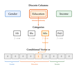
Training-by-sampling is CTGAN's elegant solution. The idea is to condition each training step on a randomly selected category, ensuring that every category – no matter how rare – receives equal attention during training.
Algorithm 2.
Training-by-Sampling with Conditional Vector
Input: Dataset with discrete columns having categories .
Compute the log-frequency of each category:
At each training iteration: enumerate[label=()]
Select a discrete column uniformly at random from .
Select a category from column with probability proportional to .
Construct the conditional vector with a 1 at the position corresponding to and zeros elsewhere.
Sample a real row uniformly from all rows in that have category in column .
Generate a fake row where .
Compute the conditional loss: verify that the generated row contains the specified category in column (via cross-entropy loss on the categorical output).
Update and using the combined loss. enumerate
The following diagram illustrates the conditional vector construction.
Key Idea.
Why training-by-sampling solves minority mode collapse. In standard GAN training, the generator encounters each category in proportion to its frequency in the dataset. A category appearing in 1% of rows is seen in roughly 1% of training iterations. With training-by-sampling, columns are sampled uniformly and categories are sampled proportional to log-frequency. The log transformation compresses the frequency ratio: if category A appears times and category B appears times, their raw frequency ratio is , but their log-frequency ratio is approximately . This dramatically increases the generator's exposure to rare categories while not completely ignoring common ones.
Moreover, the conditional vector explicitly tells the generator which category to produce. If the generator fails to produce the specified category, the cross-entropy loss on the conditional vector penalises it directly. This transforms the problem from “hope the generator discovers rare modes” to “require the generator to produce any specified mode on demand.”
Exercise 12.
Consider a dataset with a column “Disease” containing five categories with frequencies: Common Cold (), Flu (), Pneumonia (), TB (), Rare Syndrome (). Compute the raw sampling probabilities and the log-frequency sampling probabilities. By what factor is “Rare Syndrome” oversampled under the training-by-sampling scheme relative to uniform sampling from the dataset?
Remark 6.
Training-by-sampling introduces a subtle bias. Because the generator sees rare categories more often than they appear in the real data, it may overrepresent them in unconditional generation. In practice, this bias is corrected at generation time by sampling the conditional vector according to the true category frequencies rather than the log-frequency distribution used during training. This two-stage approach – oversampling during training for better mode coverage, then correcting the sampling distribution at generation time for faithful marginals – is a general principle that reappears in many later models.
Lemma 1 (Log-Frequency Oversampling Bound).
Let be the true frequency of category , and let be the log-frequency sampling probability. Then the oversampling ratio satisfies: For rare categories (), the oversampling ratio grows as , providing a logarithmic correction to the extreme undersampling that standard training would impose.
Proof.
The log-frequency probability is by definition where . The oversampling ratio is . For small , we have in typical datasets (otherwise the category has fewer than 1 expected occurrence), so . Meanwhile, is small, making the ratio large. The denominator is a constant for a given dataset, establishing the stated scaling.
The Loss Function
CTGAN combines two loss components: the adversarial loss from WGAN-GP and a conditional loss that enforces the training-by-sampling constraint.
WGAN-GP Adversarial Loss.
The adversarial training follows the Wasserstein GAN with gradient penalty framework [11]. The discriminator loss is: (DISC) where with is a random interpolation between real and fake samples, and is the gradient penalty coefficient.
Note that when PacGAN is used, the discriminator operates on packs of samples, so the Wasserstein estimate is computed over packed inputs rather than individual rows.
The generator loss consists of the adversarial component plus the conditional loss: (GEN) where is the cross-entropy loss on the conditional vector.
Conditional Cross-Entropy Loss.
Let be the conditional vector specifying that category should appear in column of the generated row. Let be the softmax output of the generator for column . Then: (COND) where is the component of corresponding to category . Since is one-hot with 1 at position , this simplifies to i.e., the negative log-probability that the generated row contains the specified category.
Definition 10 (CTGAN Combined Loss).
The CTGAN combined loss consists of the discriminator loss and the generator loss defined as: (DISC) where is the generator's predicted probability for the category specified by , and the expectations are over the sampling procedure of Algorithm 2.
Theorem 1 (Convergence of CTGAN under WGAN-GP).
Let and be the CTGAN generator and discriminator with PacGAN packing degree . Assume the following conditions hold:
The discriminator class is the set of all 1-Lipschitz functions .
The data distribution has bounded support in .
The generator has sufficient capacity to represent .
Then the WGAN-GP training procedure converges: the gradient penalty enforces an approximate 1-Lipschitz constraint on the discriminator, and at equilibrium, (Convergence) where denotes the 1-Wasserstein (Earth Mover's) distance. When , the game value equals zero. Moreover, with PacGAN packing degree , any Nash equilibrium of the game satisfies that has at least modes.
Proof.
The Wasserstein duality result follows from the Kantorovich–Rubinstein theorem: for any two distributions and on a metric space , The gradient penalty term serves as a soft constraint enforcing . Gulrajani et al. [11] showed that under mild regularity conditions, the optimal discriminator under this penalty achieves gradient norm exactly 1 almost everywhere along the interpolation path, and the training procedure converges to a local equilibrium.
For the PacGAN guarantee, observe that the packed discriminator operates on the product distribution . If the generator collapses to modes, then the packed generator distribution is supported on at most points in the product space, while the packed data distribution has a richer structure. Lin et al. [10] formalised this by showing that for packing degree , the discriminator can distinguish any generator distribution with fewer than modes from the data, so any equilibrium must have at least modes.
Exercise 13.
Show that for , the PacGAN discriminator reduces to a standard discriminator. Then consider a data distribution that is a mixture of two point masses: . Show that a standard discriminator () cannot distinguish a generator that outputs only from one that outputs , if both and are in the support of . Then show that a PacGAN discriminator with can distinguish them.
Example 8.
Gradient penalty computation in CTGAN.
Suppose a single real sample is and the corresponding fake sample is . We draw and compute the interpolation: We then compute by backpropagation through the discriminator. Suppose this gradient is with -norm . The gradient penalty for this sample is , which is small because the gradient norm is close to the target of 1.
If instead the gradient were with norm , the penalty would be , creating a strong signal to reduce the discriminator's Lipschitz constant. This self-regulating mechanism is what makes WGAN-GP training more stable than weight clipping in the original WGAN [12].
Remark 7.
The choice of for the gradient penalty coefficient was determined empirically by Gulrajani et al. [11] and has been adopted as a default in most WGAN-GP implementations, including CTGAN. Theoretical analysis by Petzka et al. [13] suggests that the penalty should scale with the dimensionality of the data, but in practice the fixed value works well across a wide range of settings. For tabular data, where the dimensionality after encoding is typically in the range –, the default is appropriate.
Exercise 14.
The gradient penalty in WGAN-GP is computed at interpolated points .
Explain why the penalty is not computed at the real and fake samples directly. (Hint: what would happen if the discriminator had gradient norm 1 at real samples but gradient norm 10 in between?)
The gradient penalty enforces rather than . Show that for the optimal discriminator (the Wasserstein potential), the gradient norm is exactly 1 almost everywhere along the transport paths between and .
Discuss how PacGAN affects the gradient penalty: when the discriminator operates on packs of samples, the input dimension is multiplied by . Does the gradient penalty need to be rescaled?
Limitations and What Comes Next
CTGAN was a watershed moment for tabular data generation, but it is not without limitations. Understanding these limitations is essential for appreciating the innovations that followed.
Limited inter-column dependency modelling.
CTGAN's generator is a fully connected network. While fully connected layers can theoretically model any function, they have no inductive bias toward capturing structured dependencies between columns. Real-world tabular data often has rich correlations: a person's income correlates with their education, which correlates with their age, which correlates with their health status. CTGAN learns these correlations implicitly through the adversarial loss, but it has no mechanism for explicitly encoding the relational structure between features.
No privacy guarantees.
CTGAN provides no formal privacy guarantees. Synthetic data generated by CTGAN may inadvertently memorise and reproduce identifiable patterns from the training data. In domains like healthcare and finance, where privacy is paramount, this is a significant limitation.
Single-table limitation.
CTGAN operates on a single flat table. Real-world databases are relational, with multiple tables linked by foreign keys. Generating coherent synthetic data across multiple related tables requires fundamentally different approaches.
Scalability.
The mode-specific normalisation preprocessing is performed once and is efficient, but the training procedure – particularly with PacGAN and WGAN-GP's gradient penalty – can be slow. The gradient penalty requires computing second-order derivatives, which is computationally expensive.
Insight.
What CTGAN got right and what it missed. CTGAN's lasting contributions are conceptual rather than architectural. The insight that tabular data requires specialised representation (mode-specific normalisation) and balanced training (training-by-sampling) has influenced every subsequent tabular generative model. Its architectural choices – vanilla fully connected layers – were adequate but not inspired. The next generation of models, starting with CTAB-GAN+, would keep CTGAN's preprocessing insights while replacing its architecture with something more powerful.
Exercise 15.
Design a simple experiment to test whether CTGAN is memorising training data. Specifically, given a trained CTGAN model and a held-out test set:
Define a metric for measuring how close generated samples are to the nearest training sample.
Propose a null hypothesis test: if the model is not memorising, what distribution would you expect for this metric?
Discuss how PacGAN with might affect memorisation.
CTAB-GAN+ – The Next Generation
If CTGAN cracked the code of representing tabular data for GANs, CTAB-GAN+ asked a bolder question: what if we could represent tabular data not just for GANs, but as something GANs already know how to generate brilliantly – images?
The idea, proposed by Zhao et al. [42], sounds almost too simple to work. Take a tabular row, reshape it into a 2D matrix, and apply the convolutional architectures that have proven spectacularly successful in image generation. Yet this seemingly naive trick, combined with careful auxiliary losses and an optional differential privacy mechanism, produces synthetic data that consistently outperforms CTGAN across a wide range of benchmarks.
The key insight is that convolutional layers have a built-in inductive bias that fully connected layers lack: they excel at capturing local interactions. When we arrange tabular features into a 2D grid, nearby features in the grid interact through convolutional kernels. If we are thoughtful about the arrangement – placing correlated features near each other – the convolutional architecture naturally captures the feature interactions that CTGAN's fully connected layers must learn from scratch.
Historical Note.
CTAB-GAN+ builds on the earlier CTAB-GAN model by the same group [14]. The “+” signifies several improvements: a more sophisticated encoder, additional loss terms, and – crucially – the integration of differential privacy via DP-SGD. In this section, we present the CTAB-GAN+ version directly, noting where it differs from its predecessor.
What CTAB-GAN+ Fixes
Before diving into the architecture, let us understand the core ideas that distinguish CTAB-GAN+ from CTGAN.
The CNN Insight.
A tabular row is naturally a 1D vector. CTGAN treats it as such and processes it with fully connected layers. CTAB-GAN+ makes a creative leap: wrap the 1D vector into a 2D matrix and process it with convolutional layers.
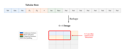
Why would this help? Consider a convolutional filter of size operating on a 2D matrix formed from a tabular row. This filter sees a local neighbourhood of features – it sees feature together with its neighbours , , and the features in adjacent rows of the matrix. If correlated features are placed near each other in the grid, the convolutional filter automatically captures their interactions. A fully connected layer, by contrast, treats all feature pairs symmetrically – it has no notion of locality.
This is the same principle that makes CNNs superior to fully connected networks for image processing: the inductive bias of locality. In images, nearby pixels are correlated; in tabular data, after careful arrangement, nearby features can also be correlated.
Definition 11 (Tabular-to-Image Encoding).
Let be the encoded representation of a tabular row (after mode-specific normalisation and one-hot encoding of categoricals). The tabular-to-image encoding is a map that reshapes into a single-channel matrix, where . If , the vector is zero-padded to length before reshaping. The dimensions and are chosen to satisfy:
is the smallest value such that both and are powers of 2 (enabling repeated up/downsampling).
Features are arranged so that correlated features occupy adjacent positions in the grid (this is typically achieved by a heuristic ordering or by grouping features from the same semantic category).
Remark 8.
The requirement that and be powers of 2 is practical rather than theoretical: it ensures that the transposed convolutions in the generator and the strided convolutions in the discriminator can cleanly halve or double the spatial dimensions at each layer, mirroring the architecture of DCGAN [15].
The following figure illustrates the tabular-to-image encoding.
Exercise 16.
Consider a tabular dataset with 42 features (after encoding). What are the smallest and (both powers of 2) such that ? How many zero-padding values are needed? Would an alternative choice (not both powers of 2) reduce the amount of padding, and what architectural complications would this cause?
The Architecture
CTAB-GAN+ consists of four components: an encoder that converts tabular rows to images, a generator that produces synthetic images from noise, a discriminator that distinguishes real from fake images, and a decoder that converts generated images back to tabular rows. The generator and discriminator follow the DCGAN architecture.
Encoder.
The encoder applies mode-specific normalisation to continuous columns and one-hot encoding to categorical columns (exactly as in CTGAN), then reshapes the resulting vector into a 2D matrix using the tabular-to-image encoding (Definition 11). The encoder is not a neural network; it is a deterministic, fixed transformation computed once during preprocessing.
Generator.
The generator follows the DCGAN transposed convolution architecture. It takes a noise vector and produces an single-channel image: (GEN) The architecture consists of a fully connected layer that maps to a small spatial feature map (e.g., ), followed by a series of transposed convolution layers with batch normalisation and ReLU activations, progressively upsampling to the target resolution: (Layer) The final layer uses a tanh activation.
Discriminator.
The discriminator is a CNN with strided convolutions, batch normalisation, and leaky ReLU activations. Critically, it has two heads:
A real/fake head that outputs a scalar score (as in standard GAN training).
An auxiliary classifier head that predicts the class label of the input (for datasets with a designated target variable).
The discriminator architecture mirrors the generator in reverse: (Layer)
Decoder.
The decoder reverses the encoder: it takes the generated image, flattens it, strips padding, and applies the inverse of mode-specific normalisation to recover tabular feature values. Like the encoder, the decoder is a deterministic function, not a neural network.
The full architecture is shown in Figure 15.
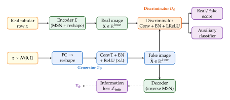
Algorithm 3.
CTAB-GAN+ Training Procedure
Preprocessing: enumerate[label=()]
Apply mode-specific normalisation to all continuous columns.
One-hot encode all categorical columns.
Concatenate into a 1D vector and reshape to image via zero-padding. enumerate
For each training epoch: enumerate[label=()]
For each mini-batch: enumerate[label=()]
Sample real images from the encoded training set.
Sample noise vectors .
Generate fake images .
Compute discriminator loss:
Update discriminator parameters .
Compute generator loss:
Update generator parameters . enumerate enumerate
Generation: enumerate[label=()]
Sample .
Generate image .
Decode back to a tabular row via the inverse encoder. enumerate
Auxiliary Classifier and Information Loss
CTAB-GAN+ introduces two loss terms beyond the standard adversarial loss: the auxiliary classifier loss and the information loss. Each addresses a specific weakness of vanilla GAN training for tabular data.
Auxiliary Classifier Loss.
Many tabular datasets have a designated target variable (e.g., “Income $50K” in the Adult dataset, “Fraud” in transaction data). Downstream machine learning tasks typically involve predicting from the other features. If the synthetic data does not preserve the conditional distribution , then classifiers trained on synthetic data will perform poorly on real test data.
The auxiliary classifier ensures class-conditional fidelity. The discriminator's auxiliary head predicts the class label from the input image (whether real or fake). This yields two loss components:
For real data: (REAL) where is the predicted probability of class .
For generated data, the generator is also trained to produce images that the auxiliary classifier labels correctly: (GEN)
The auxiliary classifier serves a dual purpose. For the discriminator, it provides a richer training signal: the discriminator must not only distinguish real from fake but also correctly classify the data, forcing it to learn semantically meaningful features. For the generator, it ensures that generated samples are not only realistic but also class-consistent.
Remark 9.
The auxiliary classifier design in CTAB-GAN+ draws inspiration from AC-GAN [16], but with an important difference. In AC-GAN, the generator receives the class label as an explicit input. In CTAB-GAN+, the class label is embedded within the tabular row itself (as one of the columns), so the generator must learn to produce coherent class labels as part of the overall row generation. The auxiliary loss provides additional supervision for this implicit conditioning.
Information Loss.
The information loss is a reconstruction penalty that ensures the generated images can be meaningfully decoded back to tabular data. Without this loss, the generator might produce images that fool the discriminator but, when decoded, yield nonsensical tabular values.
Let denote the deterministic decoder that converts a generated image back to a tabular row. The information loss has three components, one for each type of column:
For continuous columns (using mean squared error): (CONT) where is the target normalised value and is the value extracted from the generated image.
For categorical columns (using cross-entropy): (CAT) where is the target one-hot encoding and is the generated softmax output for category of column .
For mode indicators (also cross-entropy): (MODE)
The total information loss is: (Total)
Proposition 3 (Information Loss as Regulariser).
The information loss acts as a regulariser on the generator by constraining it to produce outputs in the decodable subspace of . Formally, let be the set of images that decode to valid tabular rows (i.e., continuous values in , mode indicators and categoricals forming valid probability distributions). Then minimising is equivalent to projecting the generator's output distribution onto : where is a distance function to the decodable subspace (MSE for continuous components, cross-entropy divergence for discrete components). This prevents the generator from exploiting “unreachable” regions of image space that might fool the discriminator but produce garbage when decoded.
Proof.
The decodable subspace is defined by the constraint that each generated image, when decoded, yields values consistent with the tabular encoding: normalised continuous values satisfy , mode indicators form valid probability vectors, and categorical outputs form valid probability vectors.
Consider the continuous component. The MSE loss is minimised when , which ensures the generated value lies in the valid range. For images outside , the decoded values would be inconsistent (e.g., or not summing to 1), and the information loss penalises such deviations.
The cross-entropy components similarly penalise deviations from valid discrete distributions. Since cross-entropy is minimised when , the information loss drives the generated discrete outputs toward valid one-hot encodings.
Thus, measures the distance from the generator's output to the decodable subspace under a metric that combines MSE (for continuous) and cross-entropy divergence (for discrete), and minimising it regularises the generator to stay within .
Differential Privacy Integration (DP-SGD)
One of CTAB-GAN+'s most important features is its integration with differential privacy via the DP-SGD mechanism. This is not merely a theoretical flourish; in domains like healthcare, finance, and government, the ability to provide provable privacy guarantees for synthetic data is a regulatory requirement.
Differential privacy formalises the intuitive notion that the output of a computation should not reveal too much about any single individual in the input dataset.
Definition 12 ((, )-Differential Privacy).
A randomised mechanism satisfies -differential privacy if for any two datasets that differ in exactly one record, and for any measurable subset : (DEF) The parameter is the privacy budget: smaller means stronger privacy. The parameter allows for a small probability of privacy failure.
Remark 10.
The definition says, informally, that whether or not any single individual's data is included in the dataset, the distribution of outputs changes by at most a multiplicative factor of (plus an additive ). When and , the mechanism reveals nothing about any individual – perfect privacy. As increases, the privacy guarantee weakens. Typical practical values range from (strong privacy) to (weak privacy).
The standard technique for making SGD differentially private is DP-SGD, introduced by Abadi et al. [17]. The idea is to modify each gradient update step in two ways: clip each per-sample gradient to bound its sensitivity, then add calibrated noise to the clipped sum.
Gradient Clipping.
In standard SGD, the gradient of the loss with respect to the model parameters is: where is the batch size. In DP-SGD, we first clip each per-sample gradient: (CLIP) where is the clipping norm. This ensures for all , bounding the influence of any single sample on the gradient.
Noise Addition.
After clipping, we add Gaussian noise calibrated to the clipping norm: (Noise) where is the noise multiplier. The parameter update is then .
In CTAB-GAN+, DP-SGD is applied to the discriminator's training only. The generator never sees real data directly – it only receives gradients through the discriminator – so if the discriminator's training is differentially private, the entire pipeline inherits the privacy guarantee by the post-processing property of differential privacy.
Theorem 2 (Privacy Guarantee under DP-SGD Training).
Let the CTAB-GAN+ discriminator be trained for steps with DP-SGD using clipping norm , noise multiplier , batch size , and dataset size . Define the sampling rate . Then for any , the trained generator satisfies -differential privacy, where is computed via the moments accountant: (EPS) In the regime (strong noise), this simplifies to approximately (Approx)
Proof.
The proof proceeds in three steps.
Step 1: Sensitivity. Each clipped gradient has -norm at most . Changing one record in the dataset changes at most one term in the sum, so the -sensitivity of the sum is at most (assuming the changed record is in the batch; with probability it is not sampled).
Step 2: Gaussian Mechanism. Adding to a function with -sensitivity yields -Rényi differential privacy for each step, where is the Rényi order.
Step 3: Composition via Moments Accountant. The moments accountant [17] tracks the privacy loss across training steps using the composition properties of Rényi divergence. With subsampling rate and amplification by subsampling [18], the total Rényi divergence after steps is bounded by (for the dominant term), and converting from Rényi DP to -DP via the optimal conversion formula yields the stated bound.
The post-processing property of differential privacy [19] then ensures that any function of the discriminator's parameters – including the generator's parameters, which are functions of the gradients received from the discriminator – also satisfies -differential privacy.
The following figure visualises the DP-SGD gradient clipping and noise addition process.
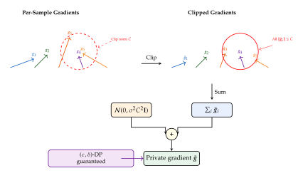
Caution.
The privacy–utility tradeoff. Differential privacy is not free. The noise added during DP-SGD degrades the gradient signal, slowing convergence and reducing the quality of the generated data. The relationship between and data utility is roughly:
: Strong privacy, significant utility loss. Generated data may fail to capture subtle correlations.
: Moderate privacy, acceptable utility for many applications.
: Weak privacy, near-full utility. But the formal guarantee is less meaningful.
: Effectively no meaningful privacy guarantee.
Practitioners must choose based on the specific privacy requirements of their application, the size of the dataset (larger datasets tolerate lower because the noise is averaged over more samples), and the acceptable loss in data utility. There is no universal “right” .
Exercise 17.
A hospital has a dataset of patient records and wants to generate synthetic data with -DP where and . They plan to train CTAB-GAN+ for steps with batch size . Using the approximate formula , compute the required noise multiplier . Then discuss qualitatively how increasing the dataset size to would affect the noise multiplier and the resulting data quality.
Exercise 18.
Prove the post-processing property of differential privacy: if satisfies -DP, and is any (possibly randomised) function, then also satisfies -DP. Explain why this property is crucial for the privacy guarantee of CTAB-GAN+: the generator is trained using gradients from the (DP-trained) discriminator, and the post-processing property ensures the generator inherits the privacy guarantee without requiring additional noise.
Experimental Results and Insights
With the architecture and training procedure established, let us examine how CTAB-GAN+ performs in practice. The original paper evaluates on five widely used benchmark datasets: Adult, Covertype, Credit, Intrusion, and Loan. These datasets span classification and regression tasks, vary in size from thousands to hundreds of thousands of rows, and include a mix of continuous, categorical, and mixed-type columns.
Evaluation Protocol.
The standard evaluation protocol for tabular generative models proceeds as follows:
Train the generative model on the real training data.
Generate a synthetic dataset of the same size.
Train downstream machine learning models (e.g., logistic regression, random forest, gradient-boosted trees) on the synthetic data.
Evaluate these models on the real test data.
Compare the test-set performance to models trained on the real training data.
The closer the “train-on-synthetic, test-on-real” (TSTR) performance is to the “train-on-real, test-on-real” (TRTR) baseline, the better the generative model.
Additionally, statistical similarity metrics are computed between the real and synthetic data distributions:
Kolmogorov–Smirnov (KS) statistic for continuous columns: measures the maximum difference between the empirical CDFs.
Jensen–Shannon divergence for categorical columns: a symmetric version of KL divergence.
Correlation structure: comparing the pairwise correlation matrix of real vs. synthetic data.
Results.
The following table summarises the key comparison between CTGAN and CTAB-GAN+ on the benchmark datasets (results from the original CTAB-GAN+ paper [42]).
| CTGAN | CTAB-GAN+ | Real | |||||
| (lr)2-4 (lr)5-7 (lr)8-8 Dataset | F1 | KS | JSD | F1 | KS | JSD | F1 |
| Adult | 0.67 | 0.08 | 0.02 | 0.72 | 0.05 | 0.01 | 0.78 |
| Covertype | 0.52 | 0.12 | 0.05 | 0.61 | 0.07 | 0.03 | 0.74 |
| Credit | 0.55 | 0.10 | 0.04 | 0.62 | 0.06 | 0.02 | 0.68 |
| Intrusion | 0.71 | 0.09 | 0.03 | 0.78 | 0.05 | 0.01 | 0.85 |
| Loan | 0.60 | 0.11 | 0.04 | 0.66 | 0.07 | 0.02 | 0.72 |
Several patterns emerge from these results:
Consistent improvement. CTAB-GAN+ outperforms CTGAN on every dataset and every metric. The ML utility gap is 5–9 F1 points, which is substantial in practical terms.
Better statistical fidelity. The KS statistics and JSD values are roughly halved, indicating that CTAB-GAN+ produces distributions much closer to the real data.
Still a gap to real data. Even CTAB-GAN+ does not close the gap to models trained on real data. The remaining 6–13 F1 point deficit suggests that there is still significant room for improvement in tabular generation.
Harder datasets benefit more. The largest improvements are on Covertype and Credit, which are the most complex datasets (many features, multiple classes, highly imbalanced). This suggests that the CNN architecture is particularly beneficial when there are many feature interactions to capture.
Key Idea.
When to use CTAB-GAN+ over CTGAN. Based on the experimental evidence and architectural analysis:
Use CTAB-GAN+ when: itemize
The dataset has many features with complex inter-column dependencies.
Privacy guarantees (DP) are required.
Downstream ML utility is the primary goal.
The dataset has a class imbalance problem and a designated target variable (the auxiliary classifier helps). itemize
Use CTGAN when: itemize
Simplicity and interpretability are paramount.
The dataset is small and simple (few features, low dimensionality).
Training speed is critical (CTGAN trains faster due to its simpler architecture).
No privacy guarantees are needed. itemize
Consider neither when the dataset is very large ( rows) or has complex relational structure (multiple tables) – in these cases, more recent methods like TVAE or diffusion-based approaches may be more appropriate.
Effect of Differential Privacy.
When DP-SGD is enabled, the ML utility drops by 3–8 F1 points depending on the privacy budget . The following qualitative relationships hold:
At : utility drops by approximately 8–12 F1 points relative to the non-private version.
At : utility drops by approximately 3–5 F1 points.
At : utility drop is less than 2 F1 points, but the privacy guarantee is weak.
These results confirm the privacy–utility tradeoff discussed in the warning box of Section Differential Privacy Integration (DP-SGD). For applications where strong privacy is required (), the utility cost is significant but may be acceptable compared to the alternative of not being able to share the data at all.
Challenge 3.
Open research question. The gap between TRTR and TSTR performance in Table 1 suggests that current tabular GANs lose significant information during the generation process. Can you identify which types of information are most likely to be lost? Some candidates:
Tail behaviour of continuous distributions (rare values far from any mode mean).
High-order interactions between three or more columns (e.g., income depends on education and work hours and occupation simultaneously).
Temporal or ordering patterns (if the original data has a time component that is lost in the flat tabular representation).
Design an experiment to disentangle these sources of information loss. How would you modify CTAB-GAN+ to address each one?
Exercise 19.
Consider the privacy accounting formula : . This reveals four “knobs” for achieving a target : , , , and .
Show that increasing the dataset size (while keeping fixed) reduces and thus reduces – i.e., larger datasets naturally provide more privacy for the same level of noise.
A data curator wants to train for twice as many steps (). By what factor must increase to maintain the same ?
Discuss why simply increasing indefinitely is not a viable strategy for achieving arbitrarily strong privacy in practice.
Exercise 20.
Implement a simplified version of the tabular-to-image encoding (Definition 11). Given a dataset with features (10 continuous, 20 binary), determine the appropriate dimensions and write pseudocode for the encoding and decoding functions. Verify that for any valid tabular row .
A Closer Look at Correlation Preservation.
One of the most informative diagnostic tools for evaluating tabular generative models is the correlation difference matrix. For each pair of features , we compute the Pearson correlation in the real data and in the synthetic data, then examine the matrix of differences .
Example 9.
Correlation preservation on the Adult dataset.
The Adult dataset has 14 features. The pairwise correlation matrix is a matrix with unique off-diagonal entries. For CTGAN, the average absolute correlation difference is approximately , meaning that correlations are on average 0.07 away from their true values. For CTAB-GAN+, this improves to .
The improvement is not uniform. CTAB-GAN+ particularly excels at preserving correlations between adjacent features in the 2D encoding – features that fall within the same convolutional receptive field. Correlations between distant features in the grid show smaller improvement, suggesting that the CNN's locality bias is both its strength and its limitation.
This observation motivates a research direction: can we design feature orderings that place maximally correlated features adjacent to each other in the 2D grid? This is equivalent to the minimum bandwidth problem in graph theory, which is NP-hard in general but admits good heuristics (such as the Cuthill–McKee algorithm) that could be applied to the feature correlation graph.
Exercise 21.
Consider the following pairwise correlation matrix for four features : You need to arrange these four features into a grid for CTAB-GAN+'s tabular-to-image encoding. A convolutional filter sees all four entries, so in this case the arrangement does not matter. Now suppose you have 16 features arranged in a grid, and the convolutional filter is . Explain why placing highly correlated features in adjacent grid positions is beneficial, and propose a greedy algorithm for finding a good arrangement.
Remark 11.
The comparison in Table 1 uses metrics that are now considered standard in the synthetic data evaluation literature, but they are not without limitations. F1 scores on downstream classifiers measure discriminative utility but say nothing about whether the synthetic data captures the full generative structure. Two synthetic datasets with the same downstream F1 could have very different joint distributions. More recent evaluation frameworks propose additional metrics [20]:
Detection score: train a classifier to distinguish real from synthetic data; a perfect synthetic dataset would yield an AUC of 0.5 (random chance).
Coverage: the fraction of real modes covered by the synthetic data.
Boundary adherence: whether the synthetic data respects known constraints (e.g., age , percentages in ).
Historical Note.
The idea of converting tabular data to images for processing by CNNs predates CTAB-GAN+. The DeepInsight method [21] proposed a similar transformation for classification tasks (not generation) in 2019. CTAB-GAN+ adapted this idea to the generative setting, combining it with GAN training, auxiliary losses, and differential privacy. The success of this approach suggests a broader principle: when a powerful architecture exists for one data modality (CNNs for images), it may be profitable to transform other data modalities into that form, even at the cost of some representational overhead (zero-padding, feature ordering heuristics). This principle has since been explored for time series, graph data, and even text.
GOGGLE – Graph-Optimized Generation
Every tabular dataset tells a hidden story about the relationships among its columns. In a medical dataset, blood pressure and age are correlated; cholesterol level depends on diet and exercise frequency; diagnosis is influenced by all of the above. These relationships form a web of dependencies that any faithful generative model must capture. Yet the methods we have studied so far, CTGAN and CTAB-GAN+, treat columns as if they were interchangeable slots in a flat vector. They rely on fully connected layers to implicitly discover column relationships from data, with no explicit mechanism for reasoning about the structure of those relationships.
This is the central insight behind GOGGLE [7]: if columns have a dependency structure, we should model that structure explicitly as a graph, and use a graph neural network (GNN) to generate data that respects the graph. The result is a method that not only generates higher-quality tabular data than previous approaches, but also produces an interpretable dependency graph that domain experts can inspect, validate, and even modify.
Let us begin with a motivating example before diving into the formalism.
Example 10 (Hospital admission data).
Consider a dataset with five columns: age,
systolic_bp, cholesterol,
exercise_hours, and diagnosis. A domain expert
would tell us that age influences both
systolic_bp and cholesterol;
exercise_hours affects cholesterol; and
diagnosis depends on systolic_bp,
cholesterol, and age. This structure is
naturally represented as a directed graph:
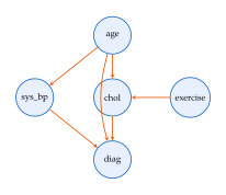
Why Graphs? The Column Dependency Problem
To understand why a graph-based approach helps, consider what happens when we use a standard fully connected generator. The generator maps a noise vector to a synthetic row through a sequence of matrix multiplications and nonlinearities. Every output dimension is connected to every input dimension through every hidden layer. This means the generator can, in principle, capture any dependency between any pair of columns.
The problem is that “in principle” and “in practice” are very different things. With columns, there are pairwise relationships, and the number of higher-order dependencies grows combinatorially. A fully connected network must allocate its limited capacity across all possible relationships, including the many that are absent or weak. The result is that the model wastes capacity on non-relationships and underfits the relationships that matter.
Insight.
Structured inductive bias. The key idea of GOGGLE is to provide a structured inductive bias: instead of asking the generator to learn column relationships from scratch, we give it a graph that encodes which columns are related. The generator then only needs to learn how related columns influence each other, not which columns are related. This is analogous to the convolutional inductive bias in image models: a CNN does not need to learn that nearby pixels are related because the architecture enforces locality. Similarly, GOGGLE does not need to learn that blood pressure depends on age because the graph encodes this dependency.
But where does the graph come from? GOGGLE offers two answers:
Learned graph: the adjacency matrix is treated as a learnable parameter and optimised jointly with the generation model.
Expert-specified graph: a domain expert provides the graph (or constraints on it), and the model generates data consistent with the specified structure.
We will explore both options in detail. First, let us formalise the architecture.
The GOGGLE Architecture
GOGGLE is a variational autoencoder (VAE) augmented with a graph neural network (GNN) that operates on the column-level dependency graph. The architecture has four components:
A graph discovery module that learns (or accepts) an adjacency matrix over the columns.
A GNN encoder that computes per-column latent representations by aggregating information from neighbouring columns according to .
A standard latent bottleneck where a variational posterior is fitted.
A GNN decoder that reconstructs each column value from the latent representation, again using message passing guided by .
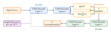
Let us now formalise each component mathematically.
Graph Discovery: Learning the Adjacency Matrix
The most novel aspect of GOGGLE is its ability to discover column relationships automatically. Rather than requiring a pre-specified graph, GOGGLE learns a soft adjacency matrix as a differentiable parameter.
Definition 13 (Learnable Adjacency Matrix).
Let be an unconstrained real-valued matrix (the “raw” adjacency parameters). The learnable adjacency matrix is defined as (ADJ) where is the element-wise sigmoid function. Each entry represents the strength of the dependency from column to column . The diagonal entries are always set to 1 (each column depends on itself).
Remark 12.
The sigmoid parameterisation ensures that all entries lie in , which has two benefits: (i) it prevents negative edge weights, which would lack a clear interpretation; (ii) it allows the model to discover soft dependencies, where a weight close to 0 means near-independence and a weight close to 1 means strong dependency. During evaluation or interpretation, one can threshold the matrix (e.g., at 0.5) to obtain a hard graph.
The adjacency matrix is trained jointly with the encoder and decoder parameters. To encourage sparsity (since real column dependencies are typically sparse), GOGGLE adds an regulariser on : (Sparse) where controls the strength of sparsification. This penalty drives weak connections toward zero, producing a clean, interpretable graph.
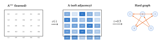
GNN Message Passing for Tabular Generation
With the adjacency matrix in hand, GOGGLE uses graph neural network layers in both the encoder and the decoder. The key idea is message passing: each column's representation is updated by aggregating information from neighbouring columns according to .
Definition 14 (GNN Message-Passing Layer).
Let denote the representation of column at layer . A single GNN message-passing layer updates this representation as follows: (MP) where are learnable weight matrices for the self-connection and neighbour aggregation respectively, is a bias vector, and is a nonlinear activation function (typically ReLU).
Remark 13.
Notice the crucial role of in (MP). If (column is not a dependency of column ), then column 's message is effectively silenced. If , the message passes at full strength. This is how the learned graph controls information flow in the network. The self-connection term ensures that each column retains its own information even if it has no neighbours (an isolated node in the graph).
The following figure illustrates message passing for a single column node.
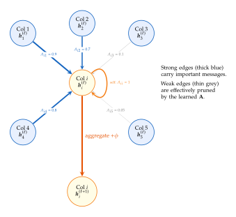
Multi-layer message passing.
By stacking GNN layers, each column can receive information from columns that are up to hops away in the dependency graph. With , column only sees its direct neighbours. With , it also sees the neighbours of its neighbours, and so on. GOGGLE typically uses layers, which provides a good balance between expressiveness and computational cost.
Proposition 4 (Receptive Field of GNN Layers).
After layers of message passing on graph , the representation of column depends on all columns such that there exists a path of length at most from to in the graph defined by . Formally, where is the -hop neighbourhood of column and is a (generally nonlinear) function determined by the GNN parameters.
Proof.
We proceed by induction on . For , the representation depends only on column 's own features, which is the 0-hop neighbourhood .
For the inductive step, assume that after layers, depends on all columns in . By (MP), aggregates for all with . Each such depends on by the inductive hypothesis. Therefore, depends on , which equals .
Example 11 (Message passing with three columns).
Consider a tiny table with three columns: age (), blood pressure (), and cholesterol (). Suppose the learned adjacency matrix after thresholding is: This encodes: bp depends on age (), cholesterol depends on age () and weakly on bp (), and age depends on nothing else. After one message-passing layer with input embeddings , the updated representations are: Observe that age's representation is updated using only its own information (no incoming edges), while cholesterol aggregates messages from both age and blood pressure, weighted by the learned dependency strengths.
Lemma 2 (Permutation Equivariance of GNN Layer).
Let be a permutation matrix acting on column indices. If we permute both the input representations and the adjacency matrix as and , then the output of the message-passing layer is permuted correspondingly: .
Proof.
This follows directly from the linearity of the aggregation. The updated representation of column (the image of under the permutation ) is: Since and summing over is the same as summing over , this equals , which is precisely the original update for column applied to the permuted inputs.
Remark 14.
Permutation equivariance means that GOGGLE does not rely on any particular ordering of columns. Reordering the columns in the dataset and correspondingly reordering the adjacency matrix produces the same results. This is a natural property for tabular data, where column ordering is arbitrary, and it distinguishes GOGGLE from MLP-based methods that are sensitive to feature ordering.
The Encoder-Decoder Architecture
With the message-passing layer defined, we can now describe the full encoder and decoder.
Encoder.
The encoder takes a real data row and maps each column value to an initial embedding: (Embed) where and are per-column embedding parameters. The initial embeddings then pass through GNN layers ((MP)), yielding final column representations .
These per-column representations are concatenated and passed through an MLP to produce the variational parameters: (MU) where is the latent dimension. A latent sample is drawn via the reparameterisation trick: (Reparam)
Decoder.
The decoder maps the latent vector back to a row reconstruction . It first splits into per-column seeds via an MLP: (Split) where each . These seeds then pass through GNN layers (with separate parameters from the encoder but using the same adjacency matrix ), producing . Finally, per-column output heads produce the reconstructed values: (Output) where is the column-specific activation: identity for continuous columns, softmax for categorical columns.
Key Idea.
Shared graph, separate parameters. The encoder and decoder use the same adjacency matrix but different weight matrices. This design choice ensures that the encoder and decoder agree on which columns are related, while allowing them to learn different transformations for the encoding and decoding directions. The shared graph acts as a structural bottleneck that forces the model to commit to a specific set of column dependencies.
The GOGGLE Loss Function
GOGGLE's training objective combines three terms: a reconstruction loss, a KL divergence term (as in any VAE), and the sparsity penalty on the adjacency matrix.
Definition 15 (GOGGLE Training Objective).
The reconstruction loss is computed per-column, using appropriate loss functions for each column type: (Recon) where and are the sets of continuous and categorical column indices respectively, and denotes the cross-entropy loss.
Remark 15.
Using per-column losses (MSE for continuous, cross-entropy for categorical) is critical. A single loss function applied uniformly to all columns would conflate very different error types. An error of 0.1 in a normalised blood pressure reading is qualitatively different from predicting the wrong diagnosis category. The per-column loss respects these differences.
Human-in-the-Loop: Expert Graph Constraints
One of the most practically valuable features of GOGGLE is its support for domain expert input. In many applications, particularly in healthcare and finance, experts have strong beliefs about which columns should (or should not) be related. GOGGLE allows these beliefs to be encoded as constraints on the adjacency matrix.
There are three types of constraints:
Must-link: columns and must be connected ( is clamped to 1).
Must-not-link: columns and must not be connected ( is clamped to 0).
Unconstrained: the model is free to learn the connection strength.
These constraints are implemented by masking the adjacency matrix during training: (MASK) where and are the sets of must-link and must-not-link pairs.
Example 12 (Expert constraints in healthcare).
A physician reviewing a synthetic patient dataset might specify:
Must-link: age blood pressure (known medical relationship).
Must-not-link: patient ID diagnosis (the ID should carry no medical information).
Unconstrained: exercise cholesterol (let the data decide).
GOGGLE incorporates these constraints and learns the remaining structure from data. The resulting graph can be shown back to the physician for validation, creating an iterative refinement loop.
Insight.
Trust but verify. The expert constraint mechanism in GOGGLE embodies a principle that is increasingly important in applied machine learning: models should be able to incorporate domain knowledge when it is available, while still being capable of autonomous discovery when it is not. This is a middle ground between fully automated black-box methods (which may discover spurious relationships) and fully expert-driven methods (which may miss non-obvious patterns). GOGGLE's interpretable graph makes it possible to verify what the model has learned, closing the loop between automated discovery and human oversight.
Training Algorithm
We now present the complete GOGGLE training procedure.
Algorithm 1: GOGGLE Training.
[htbp]
- Input: Dataset ; expert constraints , (possibly empty); hyperparameters , , learning rate , number of GNN layers
- Output: Trained parameters , ,
- Initialise , , randomly
- for each training epoch
- for each mini-batch
- Apply constraints: compute from using (MASK)
- for each
- Encode: compute per-column embeddings via (Embed)
- Run GNN encoder layers using (MP) with adjacency
- Compute , via eq:goggle:mu,eq:goggle:sigma
- Sample via reparameterisation ((Reparam))
- Decode: split into seeds via (Split)
- Run GNN decoder layers with adjacency
- Compute via (Output)
- Compute via (LOSS)
- Update Adam step with learning rate
- return , ,
Remark 16.
Note that the adjacency matrix parameters are updated by the same optimiser as the encoder and decoder parameters. The sigmoid activation and sparsity penalty together ensure that the learned graph evolves smoothly during training, with weak edges being gradually pruned. In practice, the graph stabilises after a few epochs, with the remaining training focused on improving the encoder and decoder given the fixed graph structure.
Sampling (generation).
Once training is complete, new rows are generated by:
Sampling from the prior.
Passing through the decoder (with GNN layers and the learned ) to obtain .
Applying post-processing: rounding categorical outputs to the nearest valid category; clipping continuous outputs to valid ranges.
GOGGLE vs. CTGAN: What the Graph Buys You
Having described GOGGLE in detail, let us compare it with the CTGAN approach from CTGAN – The Foundation. The comparison illuminates why explicit graph structure matters.
| Aspect | CTGAN | GOGGLE |
| Column relations | Implicit (learned by MLP) | Explicit (learned graph ) |
| [4pt] Architecture | GAN (generator + discriminator) | VAE with GNN layers |
| [4pt] Interpretability | Low (black box) | High (inspectable graph) |
| [4pt] Expert input | Not supported | Supported (must/must-not links) |
| [4pt] Training stability | GAN training can be unstable | VAE training is more stable |
| [4pt] Mode coverage | Prone to mode collapse | Better coverage (VAE + graph) |
| [4pt] Scalability | Scales well to many columns | adjacency matrix |
Caution.
The scalability caveat. GOGGLE's adjacency matrix becomes expensive when the number of columns is large (e.g., ). For very wide tables, the quadratic memory and computation cost of the adjacency matrix may outweigh the benefits of explicit graph structure. In such cases, sparse graph representations or column clustering may be necessary.
Exercise 22.
Consider a dataset with 10 columns where only 3 pairs have strong dependencies. (a) How many parameters does GOGGLE's adjacency matrix use? (b) How many of these parameters will the sparsity penalty drive to near-zero? (c) Argue informally why a fully connected MLP generator might struggle to learn the same sparse structure.
Exercise 23.
Prove that if the adjacency matrix is the identity matrix (no off-diagonal connections), then GOGGLE's GNN encoder reduces to a standard per-column MLP with no information sharing between columns. What does this imply about the quality of generated data?
Exercise 24.
Design a set of expert constraints (must-link and must-not-link)
for a financial dataset with columns: income,
credit_score, loan_amount,
default_status, zip_code,
customer_id. Explain your reasoning for each
constraint.
TabDDPM – Diffusion Models for Tabular Data
The methods we have studied so far, CTGAN, CTAB-GAN+, and GOGGLE, share a common ancestor: they are all based on either GANs or VAEs. These frameworks have served us well, but they come with well-known limitations. GANs suffer from mode collapse and training instability; VAEs tend to produce blurry reconstructions due to the Gaussian decoder assumption. Is there a fundamentally different paradigm for tabular generation?
The answer, as with so many questions in modern machine learning, comes from the world of diffusion models. In 2023, Kotelnikov et al. published TabDDPM [6], demonstrating that denoising diffusion probabilistic models (DDPMs), the same family of models that revolutionised image generation [24], can be adapted to produce state-of-the-art tabular data. The key challenge is that diffusion models, as originally conceived, operate on continuous data (images are arrays of real-valued pixel intensities), while tabular data is a mixture of continuous and categorical features. TabDDPM solves this by combining two parallel diffusion processes: Gaussian diffusion for continuous columns and multinomial diffusion for categorical columns.
The Paradigm Shift: From GANs to Diffusion
Before we dive into the technical details, let us understand why diffusion models represent a fundamentally different approach to generation.
In a GAN, the generator maps noise directly to data in a single forward pass. The challenge is that this mapping must be learned adversarially, with the generator and discriminator locked in a minimax game. The adversarial dynamics create a rich landscape of pathologies: mode collapse (the generator ignores parts of the data distribution), training oscillation (the generator and discriminator chase each other without converging), and sensitivity to hyperparameters (small changes can destabilise training entirely).
Diffusion models take the opposite approach. Instead of learning a single complex mapping, they decompose generation into a long sequence of small, simple steps. The model learns to gradually remove noise from a corrupted data point, one step at a time. Each denoising step is a simple regression problem: given a noisy input, predict the clean version (or equivalently, predict the noise that was added). There is no adversary, no minimax game, no mode collapse. The training objective is a straightforward mean squared error (for continuous data) or cross-entropy (for categorical data).
Insight.
Why diffusion avoids mode collapse. The key insight is that diffusion models are trained with a denoising score matching objective. At each noise level , the model learns to point toward the nearest mode of the data distribution. Because the training data covers all modes, the model receives gradients from all modes at every training step. There is no mechanism for the model to “forget” a mode the way a GAN generator can. This is why diffusion models consistently achieve better mode coverage than GANs.
The following figure contrasts the GAN and diffusion paradigms.
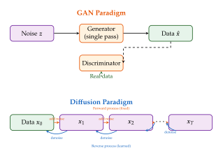
Gaussian Diffusion for Continuous Columns
Let us first describe the diffusion process for continuous features. Suppose we have a single continuous column value (we omit the column index for clarity; the process is applied independently to each continuous column).
The forward process.
The forward (noising) process gradually corrupts by adding Gaussian noise over time steps: (FWD) where is the noise schedule, a sequence of increasing values that controls how quickly the signal is destroyed.
Definition 16 (Noise Schedule).
A noise schedule is a sequence with . Two common choices are:
Linear schedule: increases linearly from to .
Cosine schedule: is derived from a cosine function, providing a gentler noise ramp that preserves signal longer in the early steps.
A crucial property of the forward process is that we can sample directly from without iterating through all intermediate steps. Define and . Then: (Closed)
Proposition 5 (Closed-Form Forward Sampling).
Proof.
We prove this by induction. For : .
For the inductive step, assume . Since , we have with independent of . Substituting yields Since and are independent Gaussians, their sum has variance . Hence .
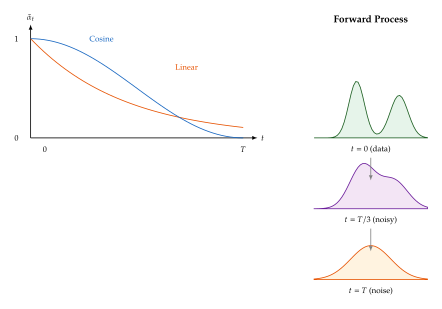
Multinomial Diffusion for Categorical Columns
The Gaussian forward process from the previous subsection works well for continuous features, but categorical features live in a discrete space. We cannot simply add Gaussian noise to a category label. TabDDPM addresses this by using multinomial diffusion [43], a diffusion process designed for categorical data.
Consider a categorical column with categories. Each value is represented as a one-hot vector with . The forward process corrupts this one-hot vector by mixing it with a uniform distribution over categories.
Definition 17 (Multinomial Forward Process).
The multinomial forward process at time step is defined as: (FWD) where is the all-ones vector and is the uniform distribution over categories. At each step, with probability the category stays the same, and with probability it is replaced by a uniformly random category.
Remark 17.
The name “multinomial diffusion” comes from the fact that the transition distribution is a categorical (multinomial with one trial) distribution. The noise process is intuitively clear: at each step, there is a small chance that the true category is “forgotten” and replaced by a random one. After sufficiently many steps, all memory of the original category is lost, and is approximately uniform over the categories.
As with Gaussian diffusion, we can derive a closed-form expression for the marginal at time : (Closed) where as before.
Proposition 6 (Closed-Form Multinomial Marginal).
Proof.
Let denote the probability vector . At , . The transition gives . Define . Then By induction, . Therefore, .
Example 13 (Multinomial diffusion in action).
Consider a categorical column “colour” with categories: red, green, blue. Suppose the true value is red, so . At time with : The true category (red) still has the highest probability, but the noise has introduced some uncertainty. At with , the distribution approaches : a uniform distribution with no memory of the original category.
The Reverse Process: Learning to Denoise Mixed Data
The forward processes (Gaussian for continuous, multinomial for categorical) define how clean data is corrupted into noise. The heart of TabDDPM is the reverse process: a neural network that learns to undo the corruption, one step at a time.
Reverse for continuous columns.
For continuous features, the reverse process at each step predicts the distribution: (CONT) where is the posterior variance (derived from Bayes' rule), and is the predicted mean, parameterised as: (MU) where is the noise prediction network. This is the standard DDPM parameterisation [24].
Reverse for categorical columns.
For categorical features, the reverse process predicts the original clean category distribution directly: (CAT) where is the network's prediction of the clean one-hot vector given the noisy input at time . This is obtained by applying Bayes' rule to the multinomial forward process.
Definition 18 (Categorical Posterior).
The posterior distribution for the categorical reverse step is: (Catpost) where denotes element-wise multiplication and the result is normalised to sum to 1.
Remark 18.
The categorical reverse process uses the “predict ” parameterisation rather than the “predict the noise” parameterisation. This is because there is no natural notion of “noise” for categorical data (unlike continuous data where noise is additive Gaussian). Instead, the network directly predicts what the original category was, and this prediction is combined with the forward process posterior to determine the next denoising step.
The Denoising Network Architecture
TabDDPM uses a single shared neural network to denoise both continuous and categorical features simultaneously. The architecture is an MLP with residual connections, specifically designed for tabular data (no convolutions, no attention).
Definition 19 (TabDDPM Denoising Network).
The denoising network is an MLP with residual blocks. Each residual block has the form: (Resblock) where is a time embedding that encodes the current diffusion time step , and is a two-layer MLP with SiLU activations and dropout.
The time embedding is computed using sinusoidal positional encoding (the same technique used in Transformers): (Timeemb) where are fixed frequencies.
The input to the network concatenates all column features (both continuous and categorical) along with the time embedding. The output has two heads:
Continuous head: predicts the noise for continuous columns.
Categorical head: predicts the clean one-hot vectors for categorical columns (via softmax).
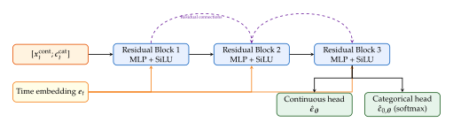
The Combined Forward Process for Mixed Data
In a real tabular dataset, continuous and categorical columns coexist. TabDDPM handles this by running Gaussian and multinomial diffusion in parallel, sharing the same noise schedule and the same time step .
Let denote a data row split into its continuous and categorical parts. The combined forward process is: (FWD) where the continuous and categorical noise processes are independent given the clean data. This independence assumption is crucial: it means we can noise each feature type using its appropriate process without worrying about cross-type interactions. The interactions are handled entirely by the shared denoising network, which sees both noisy continuous and noisy categorical features simultaneously.
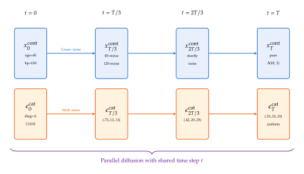
The ELBO for TabDDPM
As with all diffusion models, TabDDPM is trained by maximising an evidence lower bound (ELBO) on the log-likelihood of the data. The derivation follows the standard DDPM framework but with modifications for the mixed-type setting.
Theorem 3 (TabDDPM ELBO).
The log-likelihood of a data point is bounded below by: (ELBO) where the per-step losses decompose as: (T)
Proof.
Starting from the standard variational bound: Expanding the joint distributions as telescoping products: Using the Markov property and rearranging the ratio term by term, we rewrite the bound in terms of KL divergences between the forward posteriors and the learned reverse transitions , yielding eq:tabddpm:elbo:T,eq:tabddpm:elbo:t,eq:tabddpm:elbo:0.
Due to the independence of Gaussian and multinomial noise, the per-step KL divergences decompose further: (Decomp) where the continuous loss reduces to the standard DDPM noise prediction loss: (CONT) and the categorical loss is the KL divergence between the true and predicted categorical posteriors: (CAT)
Training Algorithm
Following the simplified training objective of [24], TabDDPM optimises a weighted sum of the per-step losses using uniform time-step sampling.
Algorithm 2: TabDDPM Training.
[htbp]
- Input: Dataset with continuous features and categorical features ; noise schedule ; denoising network
- Output: Trained parameters
- repeat
- Sample Draw a training row
- Sample Random time step
- Sample Noise for continuous
- Noise continuous features
- Sample Noise categorical features
- Compute predictions:
- Combined loss
- Update
- until converged
Remark 19.
The training procedure is remarkably simple compared to GAN training. There is no discriminator, no alternating optimisation, no careful balancing of generator and discriminator learning rates. The training is a straightforward loop: sample data, sample noise, predict, compute loss, update. This simplicity is one of the major practical advantages of diffusion models over GANs for tabular data.
Sampling (Generation)
After training, synthetic tabular rows are generated by running the reverse process from pure noise:
Algorithm 3: TabDDPM Sampling.
Caution.
Sampling is slow. The reverse process requires sequential neural network evaluations (typically ). This is much slower than GAN sampling, which requires only a single forward pass. For tabular data, this is usually acceptable because generating thousands of rows is fast even with steps (each row is low-dimensional compared to an image). However, for very large-scale generation (millions of rows), accelerated sampling methods such as DDIM [23] may be needed.
Why Diffusion Helps: Training Stability and Mode Coverage
Having described the full TabDDPM framework, let us now ask: why does it work so well? The empirical results of [6] show that TabDDPM achieves state-of-the-art performance on a wide range of tabular benchmarks, outperforming CTGAN, TVAE, and CTAB-GAN+ on most datasets. Two properties of diffusion models explain this success.
Training stability.
GAN training is fundamentally a game between two networks, and games can be unstable. The generator tries to fool the discriminator; the discriminator tries to catch the generator. If one player becomes much stronger than the other, training can collapse. Diffusion models eliminate this adversarial dynamic entirely. The training loss is a simple regression objective (MSE for continuous, cross-entropy for categorical), and the optimisation landscape is well-behaved. There is no need for gradient penalty, spectral normalisation, or other regularisation techniques that GANs require for stability.
Mode coverage.
GANs are prone to mode collapse: the generator may learn to produce data from only a subset of the data modes, ignoring the rest. This is particularly problematic for tabular data, where rare categories or unusual feature combinations represent important parts of the distribution (e.g., rare diseases in medical data). Diffusion models avoid this because their training objective is a per-sample denoising loss. Every training sample contributes equally to the loss, regardless of which mode it belongs to. The model cannot improve its loss by ignoring rare samples; it must learn to denoise all of them.
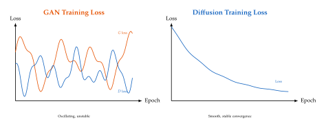
Mathematical Perspective: Continuous-Time Formulation
For the mathematically inclined reader, we briefly describe the continuous-time perspective on TabDDPM. The discrete forward process from (FWD) can be viewed as a discretisation of a stochastic differential equation (SDE).
Definition 20 (Forward SDE for Continuous Features).
The continuous-time forward process for continuous features is: (FWD) where is a continuous noise schedule function and is a standard Wiener process (Brownian motion). This is a linear SDE whose solution is an Ornstein–Uhlenbeck process.
The reverse process is given by Anderson's theorem: (REV) where is a reverse-time Wiener process and is the score function at time . The denoising network provides an estimate of the score via the relation: (Score)
Remark 20.
The continuous-time formulation reveals that diffusion models are fundamentally performing score-based generation: the learned denoising network approximates the gradient of the log data density at each noise level. This connection to score matching provides theoretical guarantees on the quality of the learned distribution and opens the door to probability flow ODEs for deterministic sampling.
Remark 21.
For categorical features, there is no direct SDE analogue (since the state space is discrete). However, recent work on continuous-time Markov chains (CTMCs) provides a similar continuous-time framework for discrete diffusion. The multinomial diffusion used by TabDDPM can be viewed as a discretisation of a CTMC where each category transitions to any other category at a rate proportional to .
Practical Considerations and Hyperparameters
Implementing TabDDPM involves several practical decisions that significantly affect performance.
Data preprocessing.
Continuous features should be normalised to have zero mean and unit variance before diffusion. This ensures that the noise schedule is appropriate for all features. Categorical features are one-hot encoded. Missing values, if present, can be handled by introducing an additional “missing” category for each categorical column or by imputing continuous values before training.
Number of diffusion steps.
The original TabDDPM paper uses steps, following the standard DDPM convention. However, tabular data is typically lower-dimensional than image data, and fewer steps (e.g., or even ) may suffice. The optimal depends on the complexity of the dataset; it should be tuned on a validation set.
Network width and depth.
The denoising MLP typically uses 3–4 residual blocks with hidden dimensions of 256 or 512. Larger networks are rarely needed for tabular data; the bottleneck is usually data quality and quantity, not model capacity.
Categorical weighting.
The relative weighting between the continuous and categorical losses (in alg:tabddpm:train, line 8) is an important hyperparameter. If is too small, the model neglects categorical features; if too large, it neglects continuous features. Cross-validation is recommended.
Key Idea.
Simplicity is a feature. One of TabDDPM's greatest strengths is its simplicity. Unlike CTGAN, which requires mode-specific normalisation, training-by-sampling, PacGAN, and Gumbel-softmax, TabDDPM uses standard diffusion with minimal tabular-specific modifications. The only adaptation is the parallel Gaussian/multinomial diffusion for mixed types. This simplicity makes TabDDPM easier to implement, debug, and extend.
Comparison with GAN-Based Methods
The following table summarises the key differences between TabDDPM and the GAN-based methods we have studied.
| Aspect | CTGAN | GOGGLE | TabDDPM |
| Framework | GAN | VAE + GNN | Diffusion |
| [3pt] Training | Adversarial (unstable) | ELBO (stable) | Denoising (very stable) |
| [3pt] Mode coverage | Prone to collapse | Good (VAE) | Excellent |
| [3pt] Mixed types | Mode-specific norm. + Gumbel-softmax | Per-column losses | Gauss. + multinomial diffusion |
| [3pt] Interpretability | Low | High (graph) | Low |
| [3pt] Sampling speed | Fast (1 pass) | Fast (1 pass) | Slow ( passes) |
| [3pt] Implementation | Complex | Moderate | Simple |
Remark 22.
No single method dominates across all dimensions. CTGAN is fast at sampling but unstable during training. GOGGLE provides interpretable graphs but scales poorly to wide tables. TabDDPM offers the best mode coverage and training stability but is slow at sampling and provides no interpretable structure. In practice, the choice depends on the specific requirements of the application: if interpretability matters, use GOGGLE; if training stability and quality matter most, use TabDDPM; if sampling speed is critical, use CTGAN.
Exercises
Exercise 25.
Consider a continuous feature with initial value and a linear noise schedule with for . (a) Compute (numerically). (b) What is the mean and variance of ? (c) At approximately what time step does the signal-to-noise ratio drop below 1?
Exercise 26.
Consider a categorical column with categories and . (a) If is the one-hot vector for category 2, compute the full probability vector . (b) Which category has the highest probability? (c) What is the entropy of compared to the uniform distribution?
Exercise 27.
Derive the categorical posterior from (Catpost) by applying Bayes' rule to the multinomial forward process. Verify that the result is a valid probability distribution (entries are non-negative and sum to 1).
Exercise 28.
Show that when there are no categorical columns (i.e., all features are continuous), the TabDDPM ELBO reduces to the standard DDPM ELBO from [24]. What simplifications occur in the loss function?
Exercise 29.
Verify the score function relation (Score). Starting from , compute and express the result in terms of the noise .
Exercise 30.
You are tasked with generating synthetic electronic health records containing 15 continuous features (lab values) and 8 categorical features (diagnosis codes, procedures). (a) Describe how you would preprocess the data for TabDDPM. (b) How would you choose the noise schedule? (c) What value of would you start with and why? (d) How would you evaluate the quality of the synthetic data?
Challenge 4.
Design a hybrid method that combines GOGGLE's interpretable graph structure with TabDDPM's diffusion framework. Specifically, propose an architecture where the denoising network uses GNN layers (guided by a learned adjacency matrix) instead of a standard MLP. Write down the forward process, the reverse process, and the training objective. What advantages would this hybrid method have over either approach alone?
A Worked Example: Two Columns, Five Steps
To solidify understanding, let us walk through a complete example of TabDDPM with a tiny dataset having one continuous column (“income”, normalised) and one categorical column (“status” with : employed, unemployed, retired).
Setup.
Consider a single data row: (normalised income), (employed). We use steps with for simplicity (so , , , ).
Forward process.
The cumulative products are: , , , , .
At , the continuous feature has distribution , meaning the signal is already heavily corrupted. The categorical feature has distribution : the true category still has the highest probability, but uncertainty is substantial.
At , , so continuous features are nearly pure noise () and categorical probabilities are , approximately uniform.
Reverse process.
Starting from noise at , the denoising network predicts the noise for continuous columns and the clean category for categorical columns at each step. Suppose at , the network predicts for income and for status. Using (MU), the denoised continuous value moves closer to the true value. Using (Catpost), the categorical posterior concentrates on “employed”. After all five reverse steps, we obtain a synthetic row that approximates the original data distribution.
Historical Note.
The idea of applying diffusion models to non-image domains gained momentum rapidly after the success of DDPM [24] in 2020. Within three years, diffusion had been applied to audio, video, 3D shapes, molecular design, protein structure, and tabular data. TabDDPM was among the first to demonstrate that diffusion could match or surpass GAN-based methods on tabular benchmarks, helping to establish diffusion as a universal framework for generative modelling rather than an image-specific technique. The breadth of this expansion is reminiscent of the GAN revolution of 2014–2018, but with notably faster adoption, likely because the training stability of diffusion models made the technology more accessible to practitioners outside the core generative modelling community.
Harpoon – Manifold-Guided Diffusion for Tabular Data
Imagine the following scenario. You have trained a diffusion model on a medical dataset containing patient demographics, lab results, and outcomes. The model generates realistic synthetic patients, and you are pleased with the quality. Then a colleague walks in and says: “I need synthetic patients who are female, over 65, with a diabetes diagnosis. Can you generate those?”
Your heart sinks. The diffusion model you trained is unconditional. It generates patients from the full joint distribution, not from the conditional distribution . The standard remedy is to retrain the model with classifier-free guidance, conditioning on the desired attributes during training. But retraining is expensive, and moreover, your colleague's conditioning requirements will change tomorrow. Perhaps she will want patients who satisfy a fairness constraint, or patients whose age falls in a specific range, or patients who match a partially observed record (missing data imputation). You cannot retrain for every conceivable condition.
This is the problem that Harpoon solves. Proposed by Liu, Seedat, Imrie, and van der Schaar [44], Harpoon enables zero-shot conditional generation from a pre-trained unconditional diffusion model. The key idea is elegant: during the reverse diffusion process, Harpoon projects intermediate samples onto a data manifold defined by the desired condition, using the manifold structure itself to guide the denoising trajectory toward the conditional distribution. No retraining, no auxiliary classifiers, no modifications to the original model.
Key Idea.
The Harpoon Principle. An unconditional diffusion model already knows the full joint distribution . The conditional distribution is a slice of that joint, living on a manifold defined by the condition . By guiding diffusion samples toward this manifold at each denoising step, we recover the conditional distribution without retraining.
Let us build up to Harpoon's algorithm step by step, starting with the fundamental challenge and progressing through the mathematical machinery.
The Challenge: Conditional Generation Without Retraining
To appreciate Harpoon's contribution, we must first understand why conditional generation from an unconditional model is hard. Recall from the theory of score-based generative models [45] that a diffusion model learns the score function: (Score) where is the marginal distribution of the noised data at time . Sampling proceeds by solving the reverse-time stochastic differential equation (SDE): (Reverse SDE) where is the drift, is the diffusion coefficient, and is a reverse-time Wiener process.
Now suppose we want to sample from the conditional distribution , where represents some condition (a set of feature values, a fairness constraint, etc.). Bayes' rule gives us the conditional score: (COND Score)
The first term on the right is precisely what our unconditional model provides. The second term, , is the guidance term. In classifier guidance [46], this term comes from a separately trained classifier. In classifier-free guidance, it is implicitly learned during training. Both approaches require training auxiliary components.
Harpoon's insight is that for many conditions of practical interest, the guidance term can be computed geometrically, without any learned classifier, by exploiting the manifold structure of the condition set.
Remark 23.
The term “zero-shot” in Harpoon's context means that the model has never seen the specific condition during training. This is distinct from the use of “zero-shot” in natural language processing, where it refers to performing a task without any task-specific examples. Here, the diffusion model is trained only once on the unconditional distribution, and all conditioning happens at inference time.
Manifold Geometry for Conditions
The key geometric idea behind Harpoon is that many conditions of practical interest define a smooth manifold (or a reasonable approximation thereof) in the data space.
Definition 21 (Condition Manifold).
Let represent a data point and let be a vector-valued condition function with . The condition manifold is the level set (Manifold) assumed to be a smooth -dimensional sub-manifold of .
Let us see how familiar conditions fit this framework.
Fixed feature values.
Suppose we want to generate data with for , where is a subset of feature indices. The condition function is for each . The condition manifold is a -dimensional hyperplane.
Range constraints.
For constraints like , the condition manifold is a slab in . While slabs have boundaries (they are manifolds with boundary), the interior is smooth and amenable to projection.
Fairness constraints.
For demographic parity, we might require that the mean outcome across protected groups be equal: , where is the protected attribute. In practice, this becomes a constraint on the generated batch, and the condition manifold has a natural geometric interpretation.
Example 14.
The geometry of a fairness constraint. Consider a two-dimensional dataset with features and a protected attribute . Suppose we want to enforce that the mean of is the same across groups: This defines a hyperplane in (the space of all generated samples), and projecting onto this hyperplane is simply a matter of adjusting the group means to match.
The following figure illustrates the concept of a condition manifold and the projection operation.
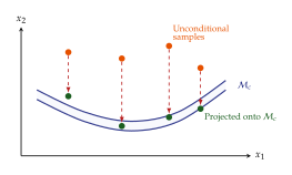
The Projection Operator
Central to Harpoon is the manifold projection operator, which maps an arbitrary point in to the nearest point on the condition manifold .
Definition 22 (Manifold Projection).
Given a point and a condition manifold , the manifold projection is (PROJ) When is a smooth sub-manifold and is sufficiently close to , the projection is unique and smooth as a function of .
For the common case where the condition is a set of fixed feature values, the projection takes an especially simple form.
Proposition 7 (Projection for Feature Fixing).
Let be a set of feature indices and be the desired feature values. The projection of onto the condition manifold is: (PROJ FIX) That is, the constrained features are replaced with their target values, and the unconstrained features are left unchanged.
Proof.
The condition manifold is the affine subspace , where is the restriction operator to indices . The orthogonal projection onto an affine subspace preserves all components orthogonal to the subspace's normal directions. The normal directions are precisely the coordinate directions for , so the projection replaces with for and leaves all other components unchanged.
For more complex conditions (nonlinear constraints, fairness conditions on batches), the projection may require iterative optimisation. Harpoon handles this through a general-purpose iterative projection sub-routine.
Algorithm 4.
Iterative Manifold Projection.
Input: Point , condition function , step size , tolerance .
Initialise: .
Repeat for : enumerate
Compute the Jacobian .
Compute the constraint residual .
Update: .
If , return . enumerate
Output: Projected point .
Remark 24.
The update rule in step 3(c) is a Gauss–Newton step applied to the nonlinear least-squares problem subject to minimising . The term is the minimum-norm solution to the linearised constraint .
Manifold Guidance: The Core Algorithm
With the projection operator in hand, we can now describe Harpoon's full guided diffusion procedure. The idea is beautifully simple: at each step of the reverse diffusion process, after the unconditional denoising update, we project the result onto the condition manifold.
But there is a subtlety. The condition manifold is defined in the clean data space , while the diffusion process operates in the noised data space at time . What does it mean to project a noised sample onto a condition manifold?
Harpoon resolves this with a two-step procedure at each diffusion step:
Denoise: Estimate the clean data point from the current noised sample using the Tweedie estimate: (Tweedie)
Project: Apply the manifold projection to the estimated clean data point: (Project Clean)
Re-noise: Map the projected clean estimate back to the noise level at the next time step : (Renoise)
The following figure illustrates how this three-step procedure guides the diffusion trajectory toward the condition manifold, compared with unguided diffusion.
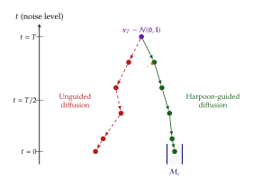
Now let us state the full Harpoon algorithm precisely.
Algorithm 5.
Harpoon: Manifold-Guided Diffusion for Conditional Generation.
Input: Pre-trained unconditional score network , condition function , noise schedule , guidance strength , number of projection steps .
Sample .
For : enumerate
Compute the unconditional score: .
Compute the Tweedie clean-data estimate: .
For : (iterative projection) itemize
. itemize
Set .
Sample .
Compute next iterate: enumerate
Output: , a sample from the approximate conditional distribution .
Insight.
Guidance strength and projection steps trade off accuracy with diversity. A large and many projection steps push the generated samples aggressively toward the condition manifold, ensuring high constraint satisfaction but potentially reducing diversity. A small with few steps preserves more of the unconditional distribution's diversity but may not perfectly satisfy the condition. In practice, Harpoon uses to and tunes by monitoring constraint violation on a validation set.
Mathematical Foundations: Guidance as Score Correction
The Harpoon algorithm may appear ad hoc at first glance: why should projecting a Tweedie estimate onto a condition manifold produce valid samples from the conditional distribution? In this subsection, we develop the theoretical justification, showing that manifold projection is a principled approximation to the exact conditional score.
Theorem 4 (Manifold Guidance as Approximate Conditional Score).
Let be the clean data distribution and let be a smooth condition manifold defined by . Assume is supported on a neighbourhood of . Let be the displacement from to its projection. Then, under suitable regularity conditions, the Harpoon guidance direction satisfies: (Guidance Approx) where the approximation holds to first order in the distance from the condition manifold.
Proof sketch.
By the implicit function theorem, near the manifold , the conditional density can be written as: where is the surface delta function on . In the noised distribution at time , this becomes: where is the surface measure on .
Taking the gradient with respect to and using the Tweedie estimate to relate to , we find that the conditional score correction is proportional to the gradient of the squared constraint function, up to terms of order that arise from the curvature of . The full details involve a Taylor expansion of the forward kernel around the projection point and careful treatment of the Jacobian of the surface measure.
This theorem has an important corollary that characterises Harpoon's convergence.
Corollary 1 (Convergence of Harpoon Sampling).
Under the assumptions of Theorem 4, let denote the distribution of samples produced by Harpoon with projection steps per diffusion step and guidance strength . Then: (Convergence) where is the unconditional score estimation error, as and is appropriately tuned, and as is the discretisation error.
Remark 25.
The bound in Corollary 1 decomposes the total error into three independent terms: how well the base model learns the unconditional distribution, how accurately the projection satisfies the condition, and how fine-grained the diffusion discretisation is. This decomposition is practically useful because it tells us where to invest computational effort: if the score model is already excellent, additional projection steps yield the most benefit.
Handling Different Condition Types
One of Harpoon's most appealing properties is its flexibility: the framework handles a wide variety of conditions through appropriate choices of the condition function and its associated projection operator . Let us catalogue the most important cases.
Definition 23 (Hard Conditioning).
A hard condition specifies exact feature values for a subset of features: where extracts the features indexed by . The projection is the simple replacement from Proposition 7.
Definition 24 (Soft Conditioning).
A soft condition specifies that features should be close to target values, with tolerance: where is the tolerance.
Definition 25 (Batch-Level Conditioning).
A batch-level condition constrains a statistic computed over a batch of generated samples : where is a feature map, is a statistic function, and is the target value.
The following figure shows the conditional generation pipeline for different condition types.
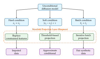
Application: Missing Data Imputation
One of Harpoon's most natural applications is missing data imputation. Given a partially observed row with missing entries indexed by , we want to sample from the conditional distribution , where is the complement of .
This is precisely a hard conditioning problem. The condition function is: (Imputation) and the projection simply replaces the observed features while letting the diffusion model “hallucinate” the missing ones.
Example 15.
Medical record imputation. Consider a patient record with features (age, blood pressure, cholesterol, BMI, diagnosis). Suppose blood pressure and cholesterol are missing. Then: Harpoon generates the missing values by:
Running the reverse diffusion process.
At each step, replacing age, BMI, and diagnosis with their observed values in the Tweedie estimate.
Allowing the diffusion model to denoise blood pressure and cholesterol freely, conditioned on the fixed features.
The result is a sample from the conditional distribution , which respects the correlations learned by the unconditional model.
Caution.
Harpoon's imputation quality depends on the unconditional model having learned accurate correlations between the observed and missing features. If the base model is poorly trained (e.g., mode-collapsed or undertrained), the imputed values may be unrealistic even if the conditioning mechanism is perfect. Always evaluate the base model's quality before using it for imputation.
Application: Fairness-Constrained Generation
A particularly compelling application of Harpoon is generating synthetic data that satisfies fairness constraints. This is a batch-level conditioning problem: we want the generated batch to exhibit demographic parity or equal opportunity across protected groups, without modifying the base model.
Definition 26 (Fairness-Constrained Generation).
Let be a binary protected attribute and be an outcome variable. The demographic parity condition on a generated batch is: (Fairness) where and .
The geometry of this constraint is illuminating. The condition manifold is a hyperplane in (the space of all generated samples), and the projection amounts to adjusting the outcome values to equalize group means.
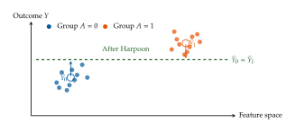
Proposition 8 (Projection for Demographic Parity).
The orthogonal projection of a batch of outcomes onto the demographic parity constraint is: (DP PROJ) where is the disparity.
Proof.
The constraint defines a hyperplane in with normal vector whose -th component is if (with appropriate sign). The orthogonal projection subtracts the component along , which distributes the correction equally across groups. A direct calculation shows this is equivalent to shifting group 0's outcomes up by and group 1's outcomes down by .
Practical Considerations and Limitations
Before leaving Harpoon, let us discuss several practical considerations that affect its deployment.
Choice of guidance strength.
The parameter controls how aggressively the diffusion path is guided toward the condition manifold. Too small, and the generated samples may violate the condition; too large, and the samples lose diversity by collapsing toward the nearest point on the manifold. A practical heuristic is to start with and adjust based on constraint violation rates.
Discrete features.
When the condition involves discrete features (e.g., “diagnosis = diabetes”), the projection must handle the discrete nature of the feature. Harpoon operates in the continuous embedding space used by the diffusion model and applies a rounding step after the final diffusion step to map continuous embeddings back to discrete categories.
Scalability.
For batch-level conditions (like fairness), the condition function and its gradient are computed over the entire batch, which can be expensive for large batches. However, since tabular datasets typically have moderate dimensionality (tens to hundreds of features), the computational overhead is manageable for batch sizes in the thousands.
Comparison with alternatives.
How does Harpoon compare with other approaches to zero-shot conditional generation? Replacement-based methods (which simply replace the conditioned features at each diffusion step without the Tweedie estimate) can produce incoherent results because they do not account for the correlation structure between features. Classifier-based guidance requires training a separate classifier for each condition. Harpoon occupies a sweet spot: it requires no auxiliary training and naturally handles the correlation structure through the unconditional model's learned score function.
Exercise 31.
Harpoon for range constraints. Consider the condition that feature should lie in the interval . Derive the projection operator for this condition and compute its Jacobian. What happens at the boundary of the interval? How does this affect the gradient of ?
Exercise 32.
Multiple simultaneous conditions. Suppose we want to generate data satisfying two conditions simultaneously: and . If the two condition manifolds and intersect transversely, explain why alternating projections onto and converge to the intersection. What goes wrong if the manifolds are nearly parallel?
Exercise 33.
Harpoon for equal opportunity. Extend the demographic parity projection from Proposition 8 to the equal opportunity constraint, which requires equal true positive rates across groups: Hint: the projection now operates only on the subset of samples with .
WaveStitch – Time Series Generation
Time series data is everywhere. Every heartbeat recorded by a wearable sensor, every stock price tick on an exchange, every temperature reading from a weather station, every packet latency measurement in a network, produces a sequence of values indexed by time. And in every one of these domains, practitioners face the same desperate need for more data: more labelled examples for anomaly detection, more diverse scenarios for stress testing, more realistic simulations for policy evaluation.
Generating synthetic time series is, in principle, just another instance of the generative modelling problem. We have a distribution over sequences , and we want to sample new sequences from a model that approximates . But in practice, time series generation is far harder than generating tabular rows or images, for reasons that we shall explore in depth.
The method we study in this section, WaveStitch, tackles one of the most challenging aspects of time series generation: producing long synthetic sequences efficiently while maintaining temporal coherence [47]. Its approach, a pipelined-parallel architecture with a novel stitching mechanism, represents a significant departure from the autoregressive and diffusion-based approaches we have encountered earlier.
Why Time Series Generation is Hard
Before diving into WaveStitch's solution, let us catalogue the challenges that make time series generation uniquely difficult. Understanding these challenges will help us appreciate why WaveStitch's design choices are necessary.
Long-range temporal dependencies.
A stock price at time depends not just on the price at but on patterns spanning days, weeks, and months. A patient's heart rate during exercise depends on the entire trajectory of exertion, not just the most recent measurement. Capturing these long-range dependencies requires models with long memory, which is computationally expensive and prone to error accumulation.
Multi-scale structure.
Real time series exhibit structure at multiple temporal scales simultaneously. An electrocardiogram (ECG) has the sub-second structure of individual heartbeats, the minute-scale structure of heart rate variability, and the hour-scale structure of circadian rhythms. A generative model must capture all scales coherently.
Non-stationarity.
Unlike images, which have (approximately) translation-invariant statistics, time series often have statistics that change over time. Financial markets have different volatility regimes. Physiological signals change with the patient's state. A model trained on one regime may produce nonsensical outputs when the regime shifts.
Periodicity and quasi-periodicity.
Many time series have periodic components (daily cycles, seasonal patterns) that must be reproduced faithfully. Slight errors in the period can compound over long sequences, leading to phase drift that destroys the temporal structure.
Length scalability.
Practitioners often need synthetic sequences that are much longer than what the model was trained on. A model trained on 256-step windows must generate sequences of 10,000 or 100,000 steps. Autoregressive generation suffers from error accumulation over long horizons; generating the entire sequence at once is computationally prohibitive.
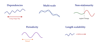
Why Naive Concatenation Fails
The most obvious approach to generating long time series is to generate short segments independently and concatenate them. If our model can produce realistic 256-step windows, why not generate forty windows and concatenate them into a 10,240-step sequence?
The answer is that the boundaries between segments create artefacts that destroy temporal coherence. Let us see why.
Suppose we generate two independent segments: Naive concatenation produces . At the boundary, we have followed by . These two values were generated independently, so there is no reason for to be consistent with the trajectory ending at .
The discontinuity is not just a matter of value mismatch; it manifests in several ways:
Level shifts: The mean of may differ from the mean of , creating a visible jump.
Slope discontinuities: Even if the values match at the boundary, the derivatives (slopes) typically do not, creating a “kink” that is immediately detectable.
Spectral artefacts: The discontinuity introduces high-frequency energy that was not present in the original signal, corrupting the spectral characteristics.
Phase breaks: For periodic signals, the phase at the start of has no relation to the phase at the end of , destroying the periodicity.
The WaveStitch Architecture
WaveStitch addresses the length scalability problem through two key innovations: a pipelined-parallel generation scheme that enables efficient production of long sequences, and a stitching mechanism that ensures seamless transitions between segments.
The high-level idea is as follows. Instead of generating one long sequence or generating independent segments, WaveStitch generates overlapping segments in parallel, where each segment shares a region of overlap with its neighbours. The shared regions are then blended using a carefully designed stitching function that preserves temporal coherence.
Definition 27 (Overlapping Segment Scheme).
Given a target sequence of length , WaveStitch generates segments of length with overlap (where ), such that: (Segments) and segment covers time steps for .
Pipelined-parallel generation.
The key efficiency insight is that segments need not be generated sequentially. WaveStitch uses a pipeline structure: once the overlap region of segment has been generated, segment can begin generating using this overlap as its prefix context. This is analogous to pipeline parallelism in computer architecture, where multiple stages of computation proceed simultaneously.
The Stitching Mechanism
The heart of WaveStitch is its stitching mechanism, which combines the overlapping regions of adjacent segments into a seamless transition. The stitching must satisfy two competing requirements:
Temporal coherence: The transition should be smooth, with no discontinuities in value, derivative, or spectral content.
Distribution preservation: The stitched region should look like it came from the same distribution as the non-overlapping regions. The stitching should not introduce artefacts that a discriminator could detect.
Definition 28 (Stitching Function).
Let and be two adjacent segments with an overlap region of length . The stitching function produces a blended overlap region: (Stitch) where is a blending weight function satisfying:
(full weight on segment at the start of overlap),
(full weight on segment at the end of overlap),
is smooth (at least , preferably ).
The choice of blending weight function is critical. WaveStitch uses a raised cosine window, which has several desirable properties.
Definition 29 (Raised Cosine Blending).
The raised cosine blending weight for the overlap region is: (Cosine) where is the position within the overlap.
Proposition 9 (Properties of Raised Cosine Blending).
The raised cosine blending weight satisfies:
and (boundary conditions).
and (zero derivative at boundaries, ensuring slope continuity).
for all (constant-power property: the sum of overlapping windows equals unity).
is .
Proof.
Properties 1 and 4 follow immediately from the definition and the smoothness of the cosine function.
For property 2, we compute: At : . At : .
For property 3: Since , the sum equals 1.
Insight.
Why the constant-power property matters. When two segments are blended, the total “energy” (variance) in the overlap region should match the energy outside the overlap. If , then the blended signal has the same expected power as the individual segments (assuming they have the same variance), preventing amplitude modulation artefacts.
The stitching mechanism is visualised in Figure 32.
Spectral Consistency
A subtle but crucial requirement for time series generation is spectral consistency: the power spectral density (PSD) of the generated sequence should match that of real sequences. Stitching artefacts, even when invisible in the time domain, can introduce spurious frequency components that are easily detected by spectral analysis.
Definition 30 (Spectral Consistency).
A generated sequence is spectrally consistent with the real distribution if: (Spectral) where is the estimated PSD of at frequency , is the true PSD, and is a frequency-dependent tolerance.
Theorem 5 (Spectral Preservation under Raised Cosine Stitching).
Let and be two segments generated from the same stationary process with PSD . The stitched signal produced by raised cosine blending satisfies: (Spectral PRES) where the error term decreases quadratically with the overlap length .
Proof sketch.
In the overlap region, the blended signal is: By the constant-power property ( with equality only at the boundaries), and assuming and are uncorrelated in the non-overlapping parts but correlated through their shared context in the overlap, the expected PSD of the blended region equals up to edge effects of order .
More precisely, the Fourier transform of the blending window has a main lobe of width and sidelobes that decay as . The convolution of the signal's PSD with the window's spectral profile introduces a bias that is bounded by the sidelobe energy.
Remark 26.
The quadratic decay in the error term explains why moderate overlap lengths () are sufficient in practice. Doubling the overlap reduces the spectral bias by a factor of four. WaveStitch typically uses to .
Cyclic Encoding for Temporal Features
Many time series carry auxiliary temporal features that exhibit cyclic structure: hour of day, day of week, month of year. These features are crucial for capturing periodicity (e.g., weekday vs. weekend traffic patterns, seasonal demand cycles), but representing them is surprisingly tricky.
The naive encoding problem.
If we encode “hour of day” as an integer from 0 to 23, the model sees hour 23 and hour 0 as maximally distant, when in fact they are one hour apart. This destroys the cyclic structure.
One-hot encoding problem.
If we one-hot encode the hours, we get a 24-dimensional binary vector that ignores the ordering and proximity of hours.
WaveStitch solves this with a cyclic encoding based on sine and cosine transformations.
Definition 31 (Cyclic Encoding).
Given a cyclic feature with period (e.g., hour with ), the cyclic encoding maps to a two-dimensional vector: (Cyclic)
This encoding has several key properties:
Proposition 10 (Properties of Cyclic Encoding).
The cyclic encoding satisfies:
Periodicity: .
Distance preservation: The Euclidean distance is a monotonic function of the minimum circular distance .
Smoothness: is .
Injectivity on one period: implies .
Proof.
Property 1 follows from the -periodicity of sine and cosine.
For property 2, by the cosine rule: where . This is a monotonically increasing function of for , which corresponds to the minimum circular distance.
Properties 3 and 4 follow from the smoothness and the fact that is injective on .
Remark 27.
Cyclic encoding can be applied to multiple temporal features simultaneously: hour of day (), day of week (), month of year (), etc. Each feature contributes two dimensions, so a time series with cyclic features gains auxiliary input dimensions. WaveStitch concatenates these cyclic encodings with the raw time series values and feeds the combined vector to the generative model.
The Complete WaveStitch Algorithm
We now assemble all components into the complete WaveStitch generation procedure.
Algorithm 6.
WaveStitch: Pipelined-Parallel Time Series Generation.
Input: Pre-trained time series generator (window length ), target length , overlap , cyclic features with periods .
Compute number of segments: .
Initialise pipeline: generate segment using with cyclic encoding of temporal position.
For (pipelined): enumerate
Extract the last steps of as the prefix context .
Compute cyclic encodings for the temporal positions of segment : .
Generate segment conditioned on prefix and temporal encodings : , where is fresh noise. enumerate
Stitch all segments using raised cosine blending: enumerate
For each overlap region between and , compute blending weights from (Cosine).
Apply (Stitch) to produce the blended overlap.
Concatenate non-overlapping parts with blended overlaps. enumerate
Output: Stitched sequence of length .
Insight.
Pipeline efficiency. If each segment takes time to generate, sequential generation of segments takes . With pipelining, the total time is approximately , where is the time to generate just the overlap region. Since (the overlap is much shorter than the full segment), the speedup is significant for large . In practice, WaveStitch achieves near-linear speedup with the number of available compute units.
Mathematical Analysis: The Overlap-and-Blend Operator
Let us formalise the overlap-and-blend operation and analyse its properties more carefully.
Definition 32 (Overlap-and-Blend Operator).
Let be a collection of segments, each of length , with overlap . The overlap-and-blend operator produces a sequence of length : (OAB) where is the partition-of-unity window for segment : (Partition) and for all .
Proposition 11 (Partition of Unity).
The windows from Definition 32 satisfy:
Proof.
At each time , at most two segments have non-zero weight (a segment and one of its neighbours in the overlap zone). In the non-overlapping region of any segment , only is active. In the overlap between segments and , we have by the constant-power property of the raised cosine window (Proposition 9, property 3).
The partition-of-unity structure guarantees that the overlap-and-blend operator is a valid averaging scheme: it never amplifies or attenuates the signal, only smoothly interpolates between adjacent segments.
Theorem 6 (Variance Preservation).
If segments and are drawn from a stationary process with variance , and the segments are conditionally independent given the overlap context, then the blended signal in the overlap region has variance: (Variance) For the raised cosine window, , achieving its minimum at (the midpoint of the overlap).
Proof.
By the definition of the stitching function ((Stitch)): For the raised cosine, , giving at the midpoint. If the segments are independent in the overlap, and the variance dips to . If they are perfectly correlated (), the variance is . In practice, the shared context creates partial correlation, and the variance is between and .
Caution.
The variance dip at the overlap midpoint (when segments are weakly correlated) can be a detectable artefact. WaveStitch mitigates this by ensuring that the shared context creates sufficient correlation between adjacent segments. If the overlap is too short relative to the correlation length of the process, the variance dip becomes pronounced. A rule of thumb is to set to be at least twice the decorrelation time of the process.
Conditional Generation for Time Series
WaveStitch's pipelined architecture naturally supports several forms of conditional generation that are particularly relevant for time series.
Prefix conditioning.
Given an observed prefix , WaveStitch can generate the continuation by using the prefix as the context for the first segment. This is forecasting, and WaveStitch's segment-based approach handles it seamlessly: the prefix simply replaces the first generated values.
Infilling.
Given observations at scattered time points, WaveStitch can fill in the gaps. Each observed value acts as a constraint on the corresponding segment. The stitching mechanism ensures that the infilled values transition smoothly between observed anchors.
Style transfer.
By conditioning the cyclic encodings on a different temporal pattern (e.g., shifting from weekday to weekend patterns), WaveStitch can transform a time series from one “style” to another while preserving the local dynamics.
Example 16.
Financial scenario generation. A risk analyst needs 10,000-step synthetic stock price paths that start from a specific price and exhibit a particular volatility regime. With WaveStitch:
Set the initial price as a prefix constraint.
Use a base model trained on the desired volatility regime.
Generate 10,000 steps using overlapping segments of length 256 with overlap 64.
The pipelined architecture generates all segments in roughly the time it takes to generate 2 segments sequentially.
The result is a long, coherent price path that respects the initial condition and exhibits realistic temporal dynamics.
Applications
WaveStitch has been applied to several domains where long, coherent synthetic time series are needed.
Healthcare monitoring.
Continuous patient monitoring generates streams of physiological data: heart rate, blood pressure, oxygen saturation, respiratory rate. Training anomaly detection models requires diverse examples of both normal and abnormal patterns, but real abnormal data is scarce. WaveStitch generates long synthetic monitoring streams that exhibit realistic transitions between normal and abnormal states, providing training data for classifiers.
Financial data.
Stress testing of financial models requires synthetic market data that exhibits realistic statistical properties (fat tails, volatility clustering, mean reversion) over long horizons. WaveStitch generates multi-thousand-step price paths that maintain these properties, enabling Monte Carlo simulations that would otherwise require prohibitively expensive real data collection.
Sensor data for IoT.
Internet-of-Things (IoT) deployments generate vast quantities of sensor data, but labelled data for fault detection is rare. WaveStitch generates synthetic sensor streams with injected anomalies, creating training datasets for predictive maintenance systems.
Energy systems.
Smart grid planning requires realistic load profiles spanning months or years. WaveStitch generates synthetic load curves that capture daily and seasonal patterns through its cyclic encoding, enabling planners to test demand response strategies on diverse scenarios.
Comparison with Alternative Approaches
How does WaveStitch compare with other approaches to long time series generation?
Autoregressive models.
Pure autoregressive generation (predicting one step at a time) suffers from error accumulation: small errors in early steps compound, causing the generated sequence to diverge from realistic trajectories. WaveStitch avoids this by generating segments in parallel, so errors do not propagate across the full sequence length.
Full-sequence diffusion.
Generating the entire sequence at once with a diffusion model ensures global coherence but requires the model to handle the full sequence length, which is computationally prohibitive for sequences of 10,000+ steps. WaveStitch achieves near-global coherence with computational cost that scales linearly with sequence length.
Simple windowed generation.
Generating non-overlapping windows and concatenating them (the naive approach from Why Naive Concatenation Fails) is fast but produces boundary artefacts. WaveStitch's overlap-and-blend mechanism eliminates these artefacts at modest additional cost.
Chronos and foundation models.
Recent foundation models for time series (like Chronos [48]) aim to learn universal representations. WaveStitch is complementary: it can use any base generator (including foundation models) for individual segments and adds the stitching layer on top.
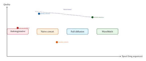
Practical Implementation Details
Several practical details affect WaveStitch's performance.
Overlap length selection.
The overlap should be chosen based on the autocorrelation structure of the data. For highly correlated processes (like smooth physiological signals), shorter overlaps suffice because the stitching artefacts are small. For processes with complex temporal structure (like financial data with regime changes), longer overlaps are needed to ensure the context carries enough information for coherent continuation.
Base model architecture.
WaveStitch is agnostic to the base generator architecture. The base model can be a diffusion model, a GAN, a VAE, or any model that can generate fixed-length time series segments conditioned on a prefix. The choice of base model affects the quality of individual segments but not the stitching mechanism.
Multi-channel time series.
For multivariate time series (multiple channels recorded simultaneously), WaveStitch applies the same stitching mechanism to all channels simultaneously, using the same blending weights. This preserves cross-channel correlations within the overlap region.
Handling distribution shift.
When generating very long sequences, the statistical properties of the data may change over time (non-stationarity). WaveStitch handles this by allowing the cyclic encodings to carry information about the current regime, enabling the base model to adapt its generation to the current temporal context.
Exercise 34.
Alternative blending functions. Consider replacing the raised cosine blending weight with a linear blending weight .
Show that linear blending satisfies the boundary conditions and .
Show that , meaning the derivative is discontinuous at the start of the overlap.
Compute the spectral leakage of the linear window and compare it with the raised cosine.
Exercise 35.
Optimal overlap length. Consider a stationary Gaussian process with autocorrelation function , where is the correlation length. Derive an expression for the variance of the stitched signal at the midpoint of the overlap as a function of and . For what value of does the variance at the midpoint equal ?
Exercise 36.
Multi-period cyclic encoding. A dataset has two temporal features: hour of day () and day of week ().
Write the full cyclic encoding vector for the timestamp “Wednesday, 3pm” (day index 3, hour 15).
Show that the encoding for “Wednesday, 11pm” is closer to “Thursday, 1am” than to “Wednesday, 3pm” in Euclidean distance.
Discuss whether this distance relationship is desirable.
Exercise 37.
WaveStitch for irregular time series. Many real-world time series are irregularly sampled (observations arrive at non-uniform time intervals). Propose a modification to WaveStitch's stitching mechanism that handles irregular sampling. Hint: consider expressing the blending weight as a function of time rather than sample index.
Exercise 38.
Error propagation analysis. Suppose the base model introduces an error (in the norm) in each segment relative to the true conditional distribution. Analyse how this error accumulates across segments under:
Naive concatenation (no overlap).
WaveStitch with overlap .
Show that WaveStitch's error grows as while naive concatenation's error grows as .
LLM-Based Tabular Generation – TabuLa
What if we could simply tell a language model to “write” a new patient record, the way we ask it to write an essay? The question sounds absurd at first. Language models are trained on books, articles, and web pages – rivers of prose – not on the orderly rows and columns of a database table. A patient record is not a sentence. It is a vector of heterogeneous features: age (continuous), blood pressure (continuous), diagnosis code (categorical), insurance type (categorical), admission date (temporal). These features live in vastly different spaces, obey complex joint distributions, and are bound by domain constraints that no amount of next-token prediction would seem to capture.
And yet, a remarkable line of research beginning around 2023 has shown that the intuition is not absurd at all. It is, in fact, correct. Language models can generate high-quality tabular data, sometimes surpassing purpose-built architectures like CTGAN and TabDDPM, provided we solve one key problem: how to represent a table row as a string that a language model can understand. This is the serialization insight, and it is the foundation of a method called TabuLa – Tabular generation via Language models [25].
The idea is disarmingly simple. Convert each row of a table into a natural-language sentence. Fine-tune a large language model on these sentences. Then sample new sentences from the fine-tuned model and parse them back into table rows. The simplicity is deceptive: behind it lies a rich set of design decisions about serialization format, padding strategy, sampling temperature, and post-processing that determine whether the method produces realistic data or incoherent gibberish.
Remark 28.
The TabuLa approach belongs to a broader movement in machine learning known as foundation models for everything. The thesis is that a single architecture (the Transformer) pre-trained on a single modality (text) contains enough inductive bias and world knowledge to handle tasks far outside its training domain, including tabular data, time series, molecular design, and even protein folding, provided the task is properly framed as a text problem. Whether this thesis is ultimately correct or whether specialized architectures will prevail remains one of the central open questions in modern AI.
The Serialization Insight
The core insight of LLM-based tabular generation is that every table row can be faithfully represented as a text string, and that language models are extraordinarily good at learning the statistical structure of text strings. If we can encode the joint distribution over features as a distribution over strings, then the language model's next-token prediction objective automatically learns the joint distribution.
Consider a simple table with three columns: age,
income, and occupation. A row
can be serialized as the string:
age is 45, income is 50000, occupation is engineer
This is the feature-value serialization format: each column name is followed by its value, and columns are separated by commas. The language model sees this as a perfectly natural English sentence (albeit a boring one) and can model the conditional distributions: simply by learning which tokens tend to follow which.
Why does this work? Three reasons converge:
Pre-trained world knowledge. A language model trained on the internet has encountered millions of sentences like “the patient is 45 years old and earns $50,000.” It already possesses statistical associations between age, income, and occupation. Fine-tuning on a specific dataset sharpens these associations but does not need to learn them from scratch.
Autoregressive factorization. The language model factors the joint distribution as: (Autoregressive) which naturally captures dependencies between features, including higher-order interactions that methods like CTGAN (which use a single noise vector) may miss.
Flexible types. Text is a universal representation. Continuous values, categorical labels, dates, free-text fields, and even missing values (serialized as “unknown” or “N/A”) all live in the same token space. No special encoding is needed for mixed types.
Definition 33 (Tabular Serialization).
Let be a tabular dataset with columns named . A tabular serialization is a deterministic function that maps each row to a string over vocabulary , such that the inverse is well-defined on the image of . The feature-value serialization takes the form: (Serialization) where converts each value to its string representation.
The invertibility requirement is crucial. If two different rows produce the same string, the language model cannot distinguish them, and the generated data will conflate distinct records. In practice, feature-value serialization is injective for all standard data types (integers, floats with fixed precision, categorical labels, dates), so invertibility holds.
Example 17 (Serializing a Medical Record).
Consider a row from a healthcare dataset: The feature-value serialization produces:
age is 67, sex is F, bp is 140, cholesterol is high,
diagnosis is hypertension
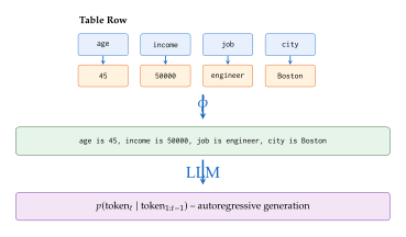
Alternative serialization formats have been explored. Some use
JSON format ("age": 45, "income": 50000), some use
comma-separated values without column names, and some use
template-based natural language (“A 45-year-old engineer in Boston
earns $50,000”). The feature-value format strikes a balance
between informativeness (column names provide context) and
compactness (minimal overhead tokens).
Exercise 39.
Consider three serialization formats for a row with column names :
Feature-value:
JSON:
Natural language: a template-based sentence embedding the values
For each format, count the number of overhead tokens (tokens not carrying feature information) for a table with columns. Which format is most token-efficient? Which format best leverages the language model's pre-training? Discuss.
TabuLa Architecture
TabuLa builds on a pre-trained large language model – specifically, LLaMA [49] – and fine-tunes it on serialized tabular data. The architecture itself is unchanged: a standard Transformer decoder with causal attention. The innovation lies entirely in the data pipeline: how rows are serialized, padded, and presented to the model.
The training procedure is straightforward in outline:
Serialize every row in the training table to a string using feature-value format.
Optionally shuffle the column order to augment data and prevent the model from relying on a fixed ordering.
Tokenize each string using the LLaMA tokenizer.
Apply middle padding to equalize sequence lengths.
Fine-tune the model using the standard causal language modelling loss: (LOSS) where denotes the model parameters and is the padded sequence length.
The column shuffling step deserves emphasis. In a standard table, columns have a fixed order (e.g., age before income before occupation). But the joint distribution is permutation-invariant: the probability of a particular combination of feature values does not depend on the order in which we list them. By randomly permuting the column order during serialization, we encourage the model to learn the true joint distribution rather than a particular autoregressive factorization. This is analogous to the order agnostic training used in XLNet [50].
Definition 34 (Middle Padding Strategy).
Let be a tokenized sequence of length and let be the target padded length. The middle padding strategy inserts padding tokens at position : (Middle Padding) The causal attention mask is modified so that padding tokens attend to nothing and are not attended to by subsequent content tokens, preserving the autoregressive property.
Why middle padding rather than the more conventional left padding (prepend pads) or right padding (append pads)? The reasoning is subtle and relates to how causal Transformers allocate attention.
Key Idea.
Why Middle Padding Outperforms Left/Right Padding. In left padding, the model must process many meaningless padding tokens before encountering any content, wasting the early layers' representational capacity on empty inputs. In right padding, the final content tokens – which carry the most recently generated features and are critical for predicting subsequent features – are far from the end-of-sequence token, making gradient flow less efficient.
Middle padding balances both concerns: the first content tokens are close to the beginning (preserving early representations), and the last content tokens are close to the end (preserving gradient flow). Empirically, middle padding improves generation quality by 3–7% across multiple datasets compared to left or right padding [25].
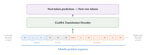
Algorithm 4 (TabuLa Training Procedure).
- Input: Training table with columns ; pre-trained LLM ; target sequence length ; learning rate ; epochs
- Output: Fine-tuned model
- Serialize:
- for each row
- random permutation of Column shuffling
- Tokenize and pad:
- for each string
- Sequence of token IDs
- Definition 34
- Fine-tune:
- for epoch
- for each mini-batch
- return
Remark 29.
The loss in Algorithm 4 masks padding tokens (via the indicator ) so that the model is not penalized for failing to predict padding. This is essential: otherwise, the model would waste capacity learning the trivial pattern of padding-follows-padding.
Sampling Strategies
Once the model is fine-tuned, generating new rows is a matter of sampling from the autoregressive distribution. But how we sample matters enormously. The standard toolkit of decoding strategies – temperature scaling, top- truncation, and nucleus (top-) sampling – all apply, but their effects on tabular data are qualitatively different from their effects on natural language.
In natural language generation, increasing the temperature makes text more creative but potentially less coherent. In tabular generation, the stakes are different:
Low temperature () produces near- deterministic outputs: the model repeats the most common rows in the training data. The generated distribution collapses to a few modes, destroying diversity and underrepresenting minority subgroups.
High temperature () produces highly diverse outputs but may generate nonsensical feature combinations: a 5-year-old with a PhD, or a blood pressure of . The generated distribution spreads too broadly, violating domain constraints.
Moderate temperature (–) typically balances diversity and validity, but the optimal value is dataset-dependent and must be tuned.
Formally, temperature scaling modifies the softmax distribution over the vocabulary at each token position: (Temperature) where is the logit for token and is the temperature.
Proposition 12 (Temperature–Diversity–Validity Trade-off).
Let denote the distribution induced by temperature over the serialized row space . Define the diversity as the entropy and the validity rate as where is the set of strings parseable to valid table rows. Then:
is strictly increasing in for .
Under mild regularity conditions (the set of valid strings has measure less than under the uniform distribution), as , which is typically vanishingly small.
There exists a temperature that maximizes , balancing diversity and validity.
Proof.
For part (1), the entropy of a temperature-scaled categorical distribution is a standard result. Write . Taking and using the identity , one shows that whenever the logits are not all equal.
For part (2), as , converges to the uniform distribution over the vocabulary at each position. The probability of generating any specific string of length approaches , so .
For part (3), both and are continuous in . As , ; as , . The product is continuous, equals zero at both extremes, and is positive for some intermediate . By the extreme value theorem, a maximum exists.
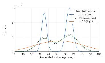
The parsing challenge is the other face of sampling. The language model produces a string, and we must convert it back to a valid table row. This requires:
Format parsing. The string must match the expected serialization format: column names in the right order, “is” separators, comma delimiters.
Type parsing. Each value must be parseable to its expected type: “45” to integer 45, “50000” to float 50000.0, “engineer” to the categorical label “engineer.”
Range checking. Parsed values must fall within valid ranges: age , blood pressure , occupation .
Rows that fail any parsing step are discarded (rejection sampling). The acceptance rate – the fraction of generated strings that survive parsing – is a key efficiency metric. At low temperatures, acceptance rates are typically 95–99%. At high temperatures, they can drop below 50%.
Exercise 40.
Suppose the serialization format for a table with columns and vocabulary size produces strings of length . Under the uniform distribution over (the limit), estimate the acceptance rate assuming each column value must match one of valid tokens. Express your answer in terms of , , and .
Few-Shot Tabular Generation
Perhaps the most remarkable capability of LLM-based tabular generation is few-shot generation: the ability to produce realistic synthetic data from just a handful of example rows, without any fine-tuning.
The mechanism is in-context learning. We provide the language model with a prompt that includes example rows (typically –) and ask it to generate more rows in the same format. The model uses its pre-trained knowledge to infer the statistical structure of the table from these examples and extrapolates.
Example 18 (Few-Shot Generation with 5 Example Rows).
The following prompt is fed to a pre-trained LLM (no fine-tuning):
Here are rows from a patient dataset: age is 45, sex is M, bp is 130, cholesterol is normal, diagnosis is healthy age is 67, sex is F, bp is 155, cholesterol is high, diagnosis is hypertension age is 32, sex is F, bp is 118, cholesterol is normal, diagnosis is healthy age is 58, sex is M, bp is 142, cholesterol is high, diagnosis is pre-hypertension age is 71, sex is M, bp is 168, cholesterol is borderline, diagnosis is hypertension Generate 3 more rows in the same format:
A capable LLM might produce:
age is 53, sex is F, bp is 138, cholesterol is borderline, diagnosis is pre-hypertension age is 29, sex is M, bp is 112, cholesterol is normal, diagnosis is healthy age is 74, sex is F, bp is 160, cholesterol is high, diagnosis is hypertension
Remarkably, the model has inferred several statistical patterns: older patients tend to have higher blood pressure; high cholesterol co-occurs with hypertension; the age distribution spans a plausible range. It achieves this from just five examples, leveraging its pre-trained medical knowledge.
Insight.
LLMs Can Learn Table Statistics From Few Examples. The success of few-shot tabular generation reveals something profound about large language models: they do not merely memorize surface patterns. They possess a form of statistical reasoning – the ability to infer distributional properties (means, variances, correlations, conditional dependencies) from a small number of observations. This is closely related to the Bayesian interpretation of in-context learning, where the model implicitly maintains a posterior over possible data-generating processes and updates it with each new example [26].
The quality of few-shot generation depends critically on several factors:
Number of examples. More examples generally improve quality, but with diminishing returns. Five to ten examples often suffice for simple distributions; complex multimodal distributions may require more.
Representative coverage. The examples should cover the diversity of the data. If all examples come from the same subgroup (e.g., only male patients), the model will undersample other subgroups.
Model size. Larger models exhibit stronger few-shot capabilities. A 7B-parameter model significantly outperforms a 350M-parameter model on few-shot tabular tasks.
Pre-training data. If the model has encountered similar tables during pre-training (e.g., medical records on the web), few-shot quality is dramatically better. This is both an advantage (leveraging world knowledge) and a risk (data leakage from pre-training).
Exercise 41.
Consider few-shot tabular generation where all example rows have . What bias would you expect in the generated data? How might you mitigate this bias while still using only 5 examples? (Hint: consider stratified sampling of the examples.)
Advantages and Limitations
The LLM approach to tabular generation brings several decisive advantages over specialized methods:
Universal type handling. Because everything is text, TabuLa handles continuous, categorical, ordinal, datetime, free-text, and even nested features without any special preprocessing. Methods like CTGAN require separate encoding for each type.
Few-shot capability. No other tabular generation method can produce reasonable outputs from five example rows. GAN-based and diffusion-based methods require hundreds to thousands of training examples.
World knowledge. The pre-trained model knows that doctors earn more than students, that blood pressure increases with age, and that “New York” is a city. This semantic knowledge improves the realism of generated data, especially for small training sets.
Flexibility. The same model can generate data for any table, in any domain, without architectural changes. Switching from healthcare to finance to ecology requires only new training data.
Conditional generation. Specifying constraints like “generate a row where age is 30 and occupation is teacher” is trivial: simply include the constraints in the prompt.
But the approach also carries significant limitations:
Computational cost. Fine-tuning a 7B-parameter model is orders of magnitude more expensive than training a CTGAN (which has 1M parameters). Generating each row requires an autoregressive pass through the entire model.
Token budget. Tables with many columns () or long text fields may exceed the model's context window. A row with 100 features might require 500+ tokens, leaving little room for few-shot examples.
Numerical precision. Language models process numbers as sequences of digit tokens. The value 3.14159 is five tokens (“3”, “.”, “14”, “15”, “9”), and the model may not capture precise numerical relationships. Rounding or binning continuous values helps but loses information.
Hallucination. The model's world knowledge is a double-edged sword. It may “hallucinate” feature combinations that are plausible in general but impossible in the specific dataset (e.g., generating a diagnosis code that does not exist in the hospital's coding system).
Caution.
LLMs Can Hallucinate Impossible Feature Combinations.
A language model fine-tuned on a corporate HR dataset may generate
an employee with title=CEO and salary=25000,
because it has seen both CEOs and low salaries in its pre-training
data but never in this particular combination. More dangerously,
it may generate medically impossible combinations (e.g., a patient
who is simultaneously pregnant and has a prostatectomy history)
that would not occur in the real data but are plausible to a model
that has learned general rather than domain-specific correlations.
Always validate generated data against domain constraints.
| Method | ML Utility | Stat. Sim. | Privacy | Speed | Few-shot |
| CTGAN | 0.78 | 0.81 | 0.65 | Fast | 55 |
| TVAE | 0.80 | 0.83 | 0.67 | Fast | 55 |
| TabDDPM | 0.86 | 0.89 | 0.72 | Moderate | 55 |
| GReaT | 0.83 | 0.85 | 0.70 | Slow | 51 |
| TabuLa | 0.84 | 0.87 | 0.71 | Slow | 51 |
Remark 30.
The comparison in Table 2 reveals a recurring theme in machine learning: there is no single best method. TabDDPM achieves the highest fidelity on large datasets. TabuLa excels in low-data regimes and offers unmatched flexibility. CTGAN remains competitive for its speed and simplicity. The choice depends on the application: if you have 100,000 rows and need high fidelity, use TabDDPM; if you have 50 rows and need quick synthetic data, use TabuLa.
Exercise 42.
A table has columns with average column name length 12 characters and average value length 6 characters. Estimate the total number of tokens per row (assuming 4 characters per token on average) for the feature-value serialization format. If the model's context window is 2048 tokens, how many few-shot examples can fit alongside one generated row?
Exercise 43.
Design a post-generation validation pipeline that detects three types of hallucinated feature combinations:
Statistical outliers (values beyond from the training distribution).
Logical inconsistencies (e.g., age 18 and marital_status = divorced).
Referential integrity violations (e.g., a department code not in the valid set).
Write pseudocode for each check.
Tabby and DeLTa – Advanced LLM Approaches
The success of TabuLa demonstrated that language models could generate tabular data. But it also exposed fundamental limitations: a single monolithic language model treats all columns identically, has no mechanism for enforcing logical constraints, and wastes parameters on the serialization overhead (column names, separators) rather than the actual data. Two lines of research address these limitations, each from a different angle.
The first, Tabby, brings the Mixture-of-Experts (MoE) paradigm to tabular language models. The insight is architectural: different columns need different expertise, and a single dense model wastes capacity by routing all information through all parameters. By allowing different subsets of parameters (“experts”) to specialize in different column types, Tabby achieves better generation quality with fewer active parameters.
The second, DeLTa, brings neurosymbolic reasoning to tabular generation. The insight is that neural models are fundamentally probabilistic – they sample from learned distributions – while domain constraints are fundamentally logical – they define hard boundaries on valid outputs. DeLTa marries the two: a neural generator proposes candidate rows, and a symbolic verifier checks and corrects them.
Together, these methods represent the cutting edge of LLM-based tabular generation, and they point toward a broader principle in AI: the best systems combine neural flexibility with symbolic correctness.
Tabby: Mixture-of-Experts for Tables
The Mixture-of-Experts (MoE) architecture, introduced by Shazeer et al. [51], replaces the single feed-forward network (FFN) in each Transformer layer with a collection of independent FFNs (“experts”) and a lightweight gating network that routes each token to the top- experts. The result is a model with many more total parameters but the same computational cost per token, because only experts are active for each token.
In natural language, MoE has been spectacularly successful: models like Mixtral [52] and Switch Transformers [53] use MoE to scale to trillions of parameters while remaining computationally tractable. But why would MoE help for tabular data?
The answer lies in the heterogeneity of table columns.
Definition 35 (Mixture-of-Experts for Tabular Generation).
A Mixture-of-Experts tabular language model replaces the feed-forward network in each Transformer layer with:
A set of expert networks , each a two-layer FFN with hidden dimension .
A gating function that produces a probability distribution over experts.
For a hidden state at any token position, the MoE layer output is: (MOE Output) where is the set of top- experts selected by the gating function: (TOPK Gating)
The gating function is the key to everything. In a well-trained MoE model, the gate learns to route different types of content to different experts. For tabular data, this means tokens corresponding to numerical values might be routed to experts that have specialized in arithmetic patterns, while tokens corresponding to categorical labels might be routed to experts that have specialized in discrete distributions.
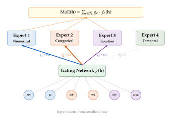
Algorithm 5 (Tabby Training with Expert Routing).
- Input: Serialized training set ; MoE model with experts and top- routing; balance coefficient ; learning rate ; epochs
- Output: Trained Tabby model
- for epoch
- for each mini-batch
- Forward pass:
- for each token position in each sequence
- Compute hidden state from attention layers
- Compute gate logits:
- Select top- experts:
- Compute MoE output:
- Compute losses:
- Language modelling loss:
- Load-balancing loss: prob for
- Total loss:
Remark 31.
The load-balancing loss is essential for MoE training. Without it, the gating network tends to collapse: it routes all tokens to one or two experts, leaving the rest unused (the “rich get richer” problem). The auxiliary loss penalizes uneven routing, encouraging all experts to receive a roughly equal share of tokens. The coefficient is typically set to –.
Why MoE Helps for Tables
To understand why MoE is particularly well-suited for tabular data, we must appreciate a fundamental difference between natural language and tables.
In natural language, every word draws on roughly the same type of knowledge: syntax, semantics, pragmatics, world knowledge. A verb needs the same fundamental processing as a noun. The heterogeneity is subtle – differences in part-of-speech, register, topic – and a dense model handles it well.
In serialized tabular data, the heterogeneity is stark. A token representing a numerical value (“45”) requires arithmetic reasoning: understanding that 45 is between 44 and 46, that it is plausible for age but implausible for blood type, that it should correlate with income in a particular way. A token representing a categorical label (“engineer”) requires discrete classification: knowing the set of valid labels, their relative frequencies, and their associations with other features. A date token (“2023”) requires temporal reasoning. These are fundamentally different computational tasks.
Proposition 13 (MoE Reduces Parameter Interference Between Column Types).
Consider a tabular language model processing a sequence containing tokens from distinct column types (numerical, categorical, temporal, etc.). In a dense model with parameters , the gradient from a numerical token and the gradient from a categorical token both update the same FFN weights, potentially causing interference: (Interference) In an MoE model, if expert specializes in numerical tokens and expert in categorical tokens, their parameters are disjoint: . Therefore: (NO Interference) The total effective capacity for each column type is preserved, as if each type had its own dedicated model.
Proof.
In the dense model, the FFN parameters are shared across all tokens. The gradient from a mini-batch is: When numerical and categorical gradients point in opposite directions in parameter space, the net gradient is diminished, slowing learning for both types.
In the MoE model, if the gating function perfectly separates types, expert receives gradients only from numerical tokens: . Since and are distinct parameter tensors, there is zero interference. In practice, the separation is soft (top- routing with ), so some interference remains, but it is significantly reduced compared to the dense baseline.
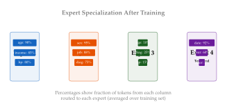
The empirical evidence supports this theoretical analysis. Tabby models with 8 experts and top-2 routing consistently outperform dense models of equivalent computational cost (matched FLOPs) on tabular generation benchmarks. The improvement is largest on tables with highly heterogeneous column types – precisely where parameter interference would be most severe.
Exercise 44.
Consider an MoE model with experts and top- routing. Each expert is a two-layer FFN with hidden dimension and input/output dimension .
What is the total number of FFN parameters in the MoE layer?
What is the number of active FFN parameters per token?
Compare with a dense FFN of the same total parameter count. What would the hidden dimension be?
Explain why the MoE model achieves better performance despite the same total parameter count, in terms of effective capacity per column type.
DeLTa: Neurosymbolic Tabular Generation
We now turn to a fundamentally different approach to improving LLM-based tabular generation. Where Tabby asks “how can we make the neural network itself better?”, DeLTa asks “what if the neural network does not need to be perfect – what if we add a checker?”
The motivation is a simple observation. Many real-world datasets come with domain constraints: logical rules that every valid record must satisfy. In a healthcare dataset, a patient listed as “pregnant” must have sex = “F.” In a financial dataset, the total of line items must equal the reported sum. In a census dataset, a person's age minus their birth year must equal the current year (approximately). These constraints are hard – they admit no exceptions – and they are symbolic – they can be expressed as logical predicates.
A purely neural generator, no matter how powerful, treats these constraints as soft statistical regularities. It learns that pregnant patients are usually female (probability ) but may occasionally generate a male pregnant patient. For many applications – healthcare, finance, government – even a 0.1% violation rate is unacceptable.
Definition 36 (Neurosymbolic Generation).
A neurosymbolic tabular generator is a system consisting of:
A neural generator that maps noise (or prompts) to candidate table rows.
A symbolic verifier that checks each candidate against a set of logical constraints and returns the set of violated constraints (empty if accepted).
The generation process is: (Neurosymbolic) Rows failing verification are either rejected (and a new candidate is drawn) or corrected by a repair module .
The name DeLTa stands for Deep Learning with Tabular constraints, emphasizing the marriage of deep learning (the neural generator) with tabular constraints (the symbolic verifier).
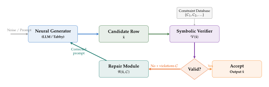
The DeLTa Pipeline
The DeLTa generation pipeline operates in three stages, forming a loop that iterates until a valid row is produced or a maximum number of attempts is reached.
Stage 1: Neural Generation.
The LLM generates a candidate row from a prompt. The prompt may include few-shot examples, column schemas, and (crucially) a natural-language description of the constraints:
Generate a patient record satisfying: age > 0, if sex is M then pregnant is No, bp_systolic > bp_diastolic.
Including constraints in the prompt provides soft guidance: the model attempts to satisfy them but is not guaranteed to succeed.
Stage 2: Symbolic Verification.
The generated row is parsed and checked against a formal constraint set . Each constraint is a logical predicate over the feature values: (Constraint Check) The row passes if and only if all constraints are satisfied: .
Stage 3: Rejection or Correction.
If the row fails verification, the system has two options:
Rejection. Discard the row and generate a new candidate. Simple but potentially wasteful if the constraint satisfaction rate is low.
Correction. Use the violated constraints to modify the row. For example, if the constraint “bp_systolic bp_diastolic” is violated with bp_systolic and bp_diastolic , the repair module can swap the values or resample bp_systolic from the conditional distribution given bp_diastolic .
The correction approach is more sample-efficient but requires a repair module that can modify individual features without destroying the overall statistical coherence of the row.
Algorithm 6 (DeLTa Generation with Symbolic Verification).
- Input: Trained neural generator ; constraint set ; max attempts ; number of rows to generate ; temperature
- Output: Generated dataset of valid rows
- while
- Generate candidate
- Convert text to row
- if failed
- continue Skip unparseable outputs
- if
- Accept valid row
- else
- for attempt
- Repair
- if
- break
- return
Example 19 (Generating Healthcare Records with Medical Constraints).
Consider generating synthetic electronic health records (EHRs) with the following constraints:
(diagnostic criterion)
The neural generator (TabuLa, fine-tuned on real EHRs) produces:
age is 34, sex is M, pregnant is Yes, bp_systolic is 125, bp_diastolic is 80, HbA1c is 5.8, diabetes is No
The symbolic verifier flags constraint 3: pregnant Yes but sex M. The repair module changes sex to F (the simpler fix, since the model's age satisfies constraint 4 for pregnancy). The corrected row:
age is 34, sex is F, pregnant is Yes, bp_systolic is 125, bp_diastolic is 80, HbA1c is 5.8, diabetes is No
This passes all constraints and is added to the synthetic dataset. Without the symbolic verifier, this medically impossible record (male pregnancy) would have entered the dataset undetected.
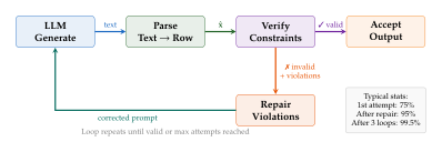
Learning and Encoding Domain Constraints
The power of the neurosymbolic approach hinges on the quality of the constraint set . Too few constraints, and invalid rows slip through. Too many, and the acceptance rate drops to the point where generation becomes impractically slow. Where do the constraints come from?
There are two complementary sources:
Expert-Specified Constraints.
Domain experts formalize their knowledge as logical rules. In healthcare, a physician might specify “if diagnosis is Type 2 Diabetes, then HbA1c 6.5” (the diagnostic criterion). In finance, an auditor might specify “total_revenue = domestic_revenue + international_revenue.” These constraints are typically few in number but high in importance – they represent hard invariants that must never be violated.
Automatically Discovered Constraints.
Given a training dataset, we can mine constraints directly from the data using techniques from database theory and data profiling:
Functional dependencies. If column determines column in the data (i.e., for all rows), this becomes a constraint: .
Range constraints. The minimum and maximum values of each numerical column define a range constraint: .
Conditional range constraints. Ranges that depend on another column: “if age , then income 100000” (a soft constraint mined from data).
Cross-column arithmetic. Relations like or can be discovered by checking arithmetic identities across all rows.
Uniqueness constraints. If a column (or combination of columns) contains only unique values in the training data, generated rows should also be unique.
Definition 37 (Tabular Constraint Language).
A tabular constraint over a table with columns is a formula in the following grammar: (Constraint Grammar 1) where is a constant value, is a set of valid values, and denotes the value of column in a given row. The constraint set is the conjunction .
This grammar is expressive enough to capture the vast majority of real-world tabular constraints (range checks, conditional rules, cross-column comparisons) while remaining computationally tractable: checking a single constraint takes time, and checking constraints takes time.
Key Idea.
Neurosymbolic Approaches Combine Neural Flexibility with Logical Correctness. The neural generator handles the “soft” aspects of generation: capturing the overall distribution, modeling complex correlations, generating realistic feature values. The symbolic verifier handles the “hard” aspects: enforcing logical constraints, checking domain rules, ensuring consistency. Neither component alone is sufficient: the neural generator without the verifier produces occasional invalid rows; the verifier without the generator has no mechanism for producing rows at all. Together, they achieve both statistical fidelity and logical correctness.
Exercise 45.
Given the following dataset fragment:
| age | employed | income | tax_bracket |
| 25 | Yes | 45000 | Low |
| 67 | No | 30000 | Low |
| 42 | Yes | 95000 | Mid |
| 17 | No | 0 | None |
| 55 | Yes | 150000 | High |
Exercise 46.
A repair module receives a row and the violated constraint .
Propose two possible repairs and discuss which is more likely to preserve the row's statistical coherence.
Formalize the repair as a constrained optimization: minimize the total change to the row (in a suitable metric) subject to all constraints being satisfied.
Show that the repair problem is NP-hard in general when constraints include arbitrary logical combinations.
The LLM Revolution in Tabular Data
We conclude this section by stepping back to survey the landscape. The evolution of tabular generation methods from 2019 to 2025 represents one of the most rapid transformations in applied machine learning: from specialized architectures designed specifically for tabular data to general-purpose language models repurposed for table generation.
Historical Note.
The Evolution from CTGAN to LLM-Based Generation (2019–2025).
The history unfolds in three acts:
Act I: The GAN Era (2019–2021). CTGAN ([4]) demonstrated that GANs could generate realistic tabular data using mode-specific normalization and a conditional generator. TVAE followed as a VAE-based alternative. These methods were fast and effective but struggled with complex distributions, rare categories, and small datasets.
Act II: The Diffusion Era (2022–2023). TabDDPM ([6]) brought denoising diffusion to tables, achieving state-of-the-art fidelity by iteratively refining noisy rows. STaSy and CoDi extended the idea with score-based and co-training approaches. Diffusion models excelled at capturing multimodal distributions but required careful handling of mixed types.
Act III: The LLM Era (2023–2025). GReaT ([27]) first showed that GPT-2 could generate table rows from serialized text. TabuLa scaled the idea to LLaMA with middle padding. Tabby added Mixture-of-Experts for heterogeneous columns. DeLTa introduced neurosymbolic verification for constraint satisfaction. The LLM approach sacrificed speed for flexibility, few-shot capability, and the ability to leverage pre-trained world knowledge.
Each era did not replace the previous one; rather, it expanded the toolkit available to practitioners. The “best” method depends on the specific use case, data size, and quality requirements.
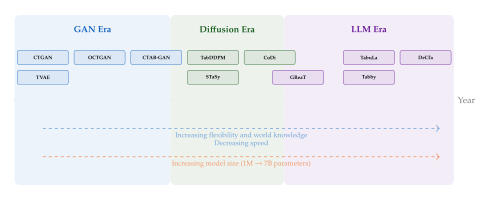
The trade-offs between these methods can be organized along several axes. Speed favours GANs and VAEs. Fidelity on large datasets favours diffusion models. Flexibility and few-shot performance favour LLMs. Constraint satisfaction favours neurosymbolic hybrids. No single method dominates on all axes – a recurring theme in machine learning that reflects the no-free-lunch theorem at a practical level.
| Method | Base LLM | Few-shot | MoE | Constraints | Params | Year |
| GReaT | GPT-2 | Partial | 55 | 55 | 124M | 2023 |
| TabuLa | LLaMA | 51 | 55 | 55 | 7B | 2023 |
| REaLTabFormer | GPT-2 | 55 | 55 | 55 | 124M | 2023 |
| Tabby | Custom | 51 | 51 | 55 | 7B | 2024 |
| DeLTa | Any | 51 | Optional | 51 | Varies | 2024 |
| Total parameters; active parameters per token are 2B with top-2 routing. | ||||||
Let us formalize the comparison along the most important dimension: sample quality versus computational cost.
Proposition 14 (Compute–Quality Pareto Frontier).
Let denote the generation quality (measured by downstream ML utility) of method , and let denote the computational cost (total FLOPs for training and generating rows). The methods form an approximate Pareto frontier in space: (COST Ordering) No method simultaneously minimizes cost and maximizes quality. The practical implication is that method selection should be driven by the application's cost and quality requirements, not by a universal “best method.”
Remark 32.
The approximate equality holds for large training sets (). For small training sets (), TabuLa's few-shot capabilities give it a decisive advantage: when is small. This is where the pre-trained world knowledge of the LLM shines.
The question of what comes next is fascinating. Several trends are visible:
Larger models. As language models scale from 7B to 70B to 400B+ parameters, their tabular generation quality will likely improve, particularly in few-shot and zero-shot settings.
Multi-table generation. Current methods generate single tables. Real databases contain multiple related tables with foreign key relationships. Generating coherent multi-table datasets is an open problem.
Privacy-preserving generation. Combining LLM-based generation with differential privacy guarantees is challenging because the pre-training data may itself contain sensitive information that “leaks” into the generated tables [28].
Interactive generation. Using conversational AI interfaces to let users specify, refine, and validate generated data in natural language: “Make the income distribution more skewed” or “Add 10% more female patients over 60.”
Challenge 5.
The Multi-Table Generation Challenge.
Consider a relational database with three tables: Patients
(patient_id, age, sex), Visits (visit_id, patient_id,
date, department), and Diagnoses (visit_id,
diagnosis_code, severity). Design a generation system that
produces synthetic data for all three tables simultaneously,
ensuring:
Referential integrity: every patient_id in
Visitsexists inPatients; every visit_id inDiagnosesexists inVisits.Cardinality constraints: each patient has between 1 and 20 visits; each visit has between 1 and 5 diagnoses.
Temporal consistency: visit dates are in chronological order for each patient and span a plausible time range.
Statistical fidelity: the marginal and joint distributions of all columns match the real data.
Discuss why autoregressive generation of serialized multi-table data is particularly challenging and propose a pipeline that addresses these requirements.
Exercise 47.
Trace the evolution of the autoregressive factorization through the three eras of tabular generation:
In CTGAN, the generator maps a single noise vector to all features simultaneously. What assumptions does this make about inter-feature dependencies?
In TabDDPM, the denoising process iteratively refines all features together. How does this differ from the autoregressive factorization?
In TabuLa, the serialization imposes an explicit left-to-right ordering. How does column shuffling mitigate the ordering bias?
In Tabby, different experts process different tokens. Does this break the autoregressive property? Why or why not?
Before stating the formal guarantees, let us examine the computational geometry of constraint satisfaction in the tabular setting.
Proposition 15 (Constraint Satisfaction as Volume Estimation).
Let be the product space of all features, and let be the subset satisfying all constraints . The constraint satisfaction rate of a generator with distribution is: (Constraint Volume) When consists of linear inequality constraints , the feasible set is a convex polytope, and can be estimated via Monte Carlo sampling from with standard error .
Proof.
The identity follows from the definition of expectation. When each constraint is a linear inequality, the intersection is a convex polytope by definition. The Monte Carlo estimator with has variance by the properties of Bernoulli random variables, giving the stated error bound.
This geometric perspective reveals why some constraint sets are harder than others. If the constraints carve out a thin sliver of the feature space (e.g., requiring that ten features simultaneously satisfy narrow bounds), the volume is tiny, and rejection sampling becomes impractical. The repair module is most valuable precisely in these high-constraint settings.
Exercise 48.
A table has continuous features, each uniformly distributed on . Consider the following constraint sets:
: (a single half-space).
: for all (a hypercube).
: (a simplex).
Compute the exact constraint satisfaction rate for each set assuming is uniform on . Which constraint set would benefit most from a repair module?
We now state the mathematical formalization of the core guarantee provided by the neurosymbolic approach.
Theorem 7 (Correctness of Neurosymbolic Generation).
Let be a neurosymbolic generator with neural component and symbolic verifier implementing constraint set . Define the constraint-satisfying set . If the generation process uses rejection sampling (accepting only rows where ), then:
Correctness: Every output row satisfies all constraints: .
Distribution: The output distribution is the conditional: (Conditional DIST) where is the distribution of the neural generator.
Efficiency: The expected number of samples from to produce one accepted row is: (Rejection Efficiency)
Proof.
Part (1) follows directly from rejection sampling: only rows passing all constraints are accepted, so by construction.
For part (2), rejection sampling produces the conditional distribution of restricted to . For any :
For part (3), the number of attempts until the first acceptance is a geometric random variable with success probability , giving .
Remark 33.
Theorem 7 highlights a crucial efficiency concern. If the neural generator's constraint satisfaction rate is low (say 1%), then each accepted row requires 100 generation attempts on average. This is why the repair module is valuable: by correcting constraint violations rather than rejecting outright, it effectively increases and reduces the number of full generation calls needed.
Lemma 3 (Repair Module Improves Efficiency).
Let be the constraint satisfaction rate of the raw neural generator and the probability that the repair module successfully corrects a violated row. Then the effective acceptance rate with repair is: (Repair Efficiency) and the expected number of generation-repair cycles to produce one valid row is: (Repair Attempts) For and , this gives and .
Proof.
A row is accepted in one cycle if either (a) the neural generator produces a valid row (probability ) or (b) the generator produces an invalid row (probability ) and the repair module fixes it (probability ). These events are mutually exclusive (case (b) only applies when (a) fails), so . The number of cycles is geometric with success probability .
Exercise 49.
Extend Lemma 3 to the case where the repair module is applied iteratively up to times per generated row. Let be the probability that repair succeeds on the -th attempt given it failed on attempts .
Derive the effective acceptance rate as a function of and .
Under the simplifying assumption that for some decay factor (each repair attempt is less likely to succeed than the previous one), find the optimal that minimizes total computation (generation + repairs per cycle, averaged over cycles).
Compute for , , , and .
The following corollary ties together the efficiency analysis with a practical stopping criterion.
Proposition 16 (Confidence Bound on Validity Rate).
After generating candidate rows and observing valid rows (before repair), the empirical validity rate is . A -confidence lower bound on the true validity rate is given by the Clopper–Pearson interval: (Clopper Pearson) where is the inverse of the regularized incomplete Beta function. This bound is useful for deciding whether the neural generator's quality is sufficient for practical deployment or whether the constraint set needs to be relaxed.
Remark 34.
In practice, a validity rate below 50% suggests that the neural generator and the constraint set are poorly matched: either the generator needs further fine-tuning on constraint-satisfying data, or the constraints are too restrictive for the generator's learned distribution. The Clopper–Pearson bound provides a principled way to detect this situation early, before wasting computational resources on a large generation run.
The interplay between neural generation and symbolic verification that DeLTa embodies is not unique to tabular data. It reflects a broader principle in AI that has been recognized since the earliest days of the field: the tension between connectionism (learning patterns from data) and symbolicism (reasoning from rules). The genius of the neurosymbolic approach is that it does not take sides. It lets each paradigm do what it does best – the neural network generates, the symbolic system verifies – and combines them in a way that is more than the sum of its parts.
Insight.
The Neurosymbolic Principle. In any domain where the data distribution is complex (requiring neural flexibility) but the output must satisfy hard constraints (requiring logical guarantees), a neurosymbolic architecture outperforms purely neural or purely symbolic approaches. The neural component provides coverage (the ability to produce diverse, realistic outputs). The symbolic component provides correctness (the guarantee that outputs satisfy specified constraints). Neither alone achieves both. This principle extends beyond tabular data to program synthesis, theorem proving, robotic planning, and drug design.
Exercise 50.
The neurosymbolic principle applies to domains beyond tabular generation. For each of the following, describe what the “neural generator” and “symbolic verifier” would be:
Program synthesis. An LLM generates code; a type checker verifies type correctness.
Molecular design. A generative model proposes molecules; a physics simulator checks stability.
Robotic planning. A neural planner proposes action sequences; a constraint solver verifies collision avoidance and joint limits.
For each domain, estimate whether the constraint satisfaction rate is high or low, and discuss the implications for the efficiency of the neurosymbolic pipeline.
Exercise 51.
Implement a simplified DeLTa pipeline in pseudocode that:
Uses a language model API to generate candidate rows from a prompt containing 5 few-shot examples and 3 constraints.
Parses the generated text into a dictionary of column name value pairs.
Checks three constraints: (a) age , (b) income , (c) if employed No then income .
Implements a simple repair module that clips out-of-range values and sets income to 0 if employed No and income .
Generates 100 valid rows, tracking the acceptance rate before and after repair.
We have now traversed the full landscape of LLM-based tabular generation, from the simple serialization insight of TabuLa through the architectural innovations of Tabby's Mixture-of-Experts to the neurosymbolic guarantees of DeLTa. The journey illustrates a broader trend in AI: the convergence of large language models with domain-specific structure. Language models provide the statistical backbone – the ability to learn and sample from complex distributions over sequences. Domain structure provides the guardrails – the constraints, types, and relationships that distinguish valid outputs from hallucinated noise. The most powerful systems combine both.
TabStruct – Evaluating Structural Fidelity
We have now studied an impressive arsenal of generative methods for tabular data: CTGAN, CTAB-GAN+, TabDDPM, GReaT, TabuLa, and several more. Each method claims to produce “realistic” synthetic tables. But what does “realistic” actually mean? How do we know whether a synthetic table is good enough to use in practice? And, perhaps more importantly, how do we compare two methods to decide which one is better?
These questions sound simple. They are not. In fact, evaluation is arguably the hardest unsolved problem in tabular data generation. The difficulty stems from a fundamental asymmetry: generating synthetic data requires learning a single distribution, but evaluating synthetic data requires comparing two distributions, the real and the synthetic, across an enormous number of dimensions simultaneously. A synthetic table might perfectly reproduce marginal distributions but completely destroy pairwise correlations. It might preserve correlations but introduce subtle privacy leaks. It might pass every statistical test yet prove useless for training a downstream classifier.
The field has struggled with this problem for years, and the result has been a chaotic landscape of ad hoc metrics, inconsistent benchmarks, and papers that cherry-pick evaluation criteria to favour their own methods. Into this landscape stepped TabStruct, a framework introduced by Liu, Kolossov, Yoon, and van der Schaar in 2025 [54], which proposed a principled, hierarchical approach to evaluating the structural fidelity of synthetic tabular data.
In this section, we dissect the evaluation crisis, explain TabStruct's solution, formalise each metric mathematically, and build intuition for why structural fidelity matters more than any single summary statistic.
Key Idea.
A single number cannot capture the quality of synthetic data. Evaluation must be hierarchical: we need metrics at the column level, the pairwise level, the table level, the task level, and the privacy level. TabStruct's contribution is to organise these levels into a coherent framework and to show that methods which score well on simple metrics can fail catastrophically on structural ones.
The Evaluation Crisis
To appreciate why evaluation is so difficult, consider a concrete
example. Suppose we have a medical dataset with three columns:
age (continuous), diagnosis (categorical), and
treatment_cost (continuous). In the real data, older
patients are more likely to have certain diagnoses, and those
diagnoses are associated with higher treatment costs. The joint
distribution has a
complex, multi-modal structure.
Now suppose we evaluate a synthetic dataset using only marginal distributions. The synthetic data might perfectly reproduce the distribution of ages, the distribution of diagnoses, and the distribution of costs, each considered in isolation. Every column looks perfect. But if the synthetic data assigns treatment costs uniformly at random, independent of diagnosis, then the crucial three-way structure is destroyed. A model trained on this synthetic data to predict treatment costs from age and diagnosis would perform terribly on real data.
Example 20.
Consider a dataset where of patients with diagnosis “diabetes” have treatment costs above $10,000, while of patients with diagnosis “common cold” have costs below $500. A synthetic dataset that preserves the marginal distribution of costs and the marginal distribution of diagnoses but destroys the correlation between them would show roughly the same fraction of high-cost and low-cost entries, and the same fraction of diabetes and cold entries, but would assign high costs to cold patients and low costs to diabetes patients at roughly equal rates. The marginals are perfect; the structure is garbage.
This example illustrates the core problem: marginal fidelity does not imply structural fidelity. Yet many early papers in tabular data generation evaluated their methods using only column-wise metrics, creating a misleading picture of progress.
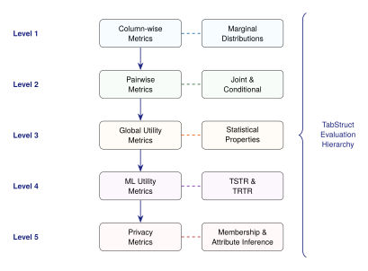
The evaluation crisis manifests in several concrete ways:
Metric shopping: researchers report only the metrics on which their method performs best, omitting others.
Inconsistent baselines: different papers compare against different methods, often using different hyperparameters, making cross-paper comparison impossible.
Tiny benchmarks: many papers evaluate on only 2–3 datasets, often the same ones (Adult, Covertype, Intrusion), providing limited evidence for generalisation.
Missing privacy analysis: papers that claim to produce “privacy-preserving” synthetic data often provide no formal privacy guarantees and no empirical privacy evaluation.
TabStruct addresses these problems by defining a comprehensive, standardised evaluation protocol that spans five levels. We now examine each level in detail.
Column-Wise Metrics: Marginal Fidelity
The simplest question we can ask about synthetic data is: does each column, considered individually, look like the corresponding column in the real data? This is the question of marginal fidelity.
For a continuous column with real distribution and synthetic distribution , we measure marginal fidelity using the Kolmogorov–Smirnov (KS) statistic:
Definition 38 (Kolmogorov–Smirnov Statistic).
Let and be the empirical cumulative distribution functions of the real and synthetic samples for a given column. The KS statistic is: (KS) A smaller value indicates better marginal fidelity. Under the null hypothesis that the two samples come from the same distribution, the KS statistic converges to zero at rate .
For categorical columns, the natural analogue is the Total Variation Distance (TVD), also known as the distance between probability vectors:
Definition 39 (Total Variation Distance).
Let and be probability distributions over a finite set of categories. The total variation distance is: (TVD)
Remark 35.
The factor of ensures that . A TVD of means the distributions are identical; a TVD of means they have disjoint support.
TabStruct computes these metrics for every column and reports both the per-column values and an aggregate (typically the mean). The per-column breakdown is crucial: a method might achieve excellent average KS scores while completely failing on one or two important columns.
Pairwise Metrics: Joint and Conditional Fidelity
Column-wise metrics, as we have argued, are necessary but not sufficient. The next level asks: for every pair of columns , does the joint distribution in the synthetic data match that of the real data?
For two continuous columns, we can measure the discrepancy between their joint distributions using the pairwise correlation difference:
(CORR DIFF)
where denotes the Pearson correlation coefficient. While simple, this metric captures only linear relationships. TabStruct also employs the contingency similarity for pairs involving categorical columns and the mutual information difference for a more general measure:
(MI DIFF)
where is the mutual information between columns and .
Insight.
Mutual information captures both linear and non-linear dependencies. Two columns might have zero Pearson correlation yet high mutual information (e.g., with ). For tabular data, where non-linear relationships are common, mutual information is a more reliable metric than correlation.
For mixed pairs (one continuous, one categorical), TabStruct computes the conditional distribution distance. Given a categorical column and continuous column , we partition the samples by category and compare the conditional distributions:
(COND DIST)
This is a weighted average of KS distances, where each weight is the real frequency of category . A synthetic dataset could have perfect marginal distributions for both and while having large : the per-category distributions of might be scrambled.
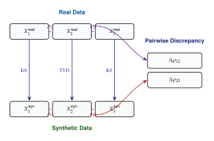
The pairwise correlation matrix provides a particularly revealing visualisation. For a table with columns, we compute the correlation matrix for both the real and synthetic data, then examine the element-wise difference. A good synthetic generator produces a difference matrix close to zero everywhere.
Definition 40 (Correlation Matrix Distance).
Let and be the correlation matrices of the real and synthetic data. The correlation matrix distance is: (CORR Matrix DIST) This is the mean absolute difference over all unique pairs.
Exercise 52.
Consider a dataset with four columns: independent, with , and a categorical column with categories where the probability of depends on . A synthetic generator produces data with correct marginals for all four columns but generates independently of and . Compute the approximate correlation matrix distance and the conditional distribution distance .
Global Utility Metrics
Global utility metrics ask a broader question: does the synthetic dataset, taken as a whole, preserve the statistical properties of the real dataset? While column-wise and pairwise metrics decompose quality into individual components, global utility takes a holistic view.
The most fundamental global utility metric is based on the Maximum Mean Discrepancy (MMD), a kernel-based distance between distributions:
Definition 41 (Maximum Mean Discrepancy).
Let be a reproducing kernel Hilbert space (RKHS) with kernel . The MMD between distributions and is: (MMD) When is a characteristic kernel (e.g., the Gaussian RBF kernel), if and only if [29].
In practice, we estimate the MMD using an unbiased estimator over finite samples and :
(MMD EST)
The MMD is attractive because it captures differences in all moments of the distributions simultaneously, not just means or variances. However, it requires careful kernel selection. For tabular data, TabStruct recommends using a mixture of RBF kernels with multiple bandwidth parameters to capture structure at different scales.
Remark 36.
The MMD has a computational cost of due to the pairwise kernel evaluations. For large datasets, approximate methods based on random Fourier features [30] can reduce this to where is the number of random features.
Another important global utility metric is the log-cluster metric, which measures whether the real and synthetic data form distinct clusters or overlap naturally:
Definition 42 (Log-Cluster Metric).
Label all real samples as and all synthetic samples as . Train a logistic regression classifier on this combined dataset. The log-cluster metric is: (Logcluster) If the synthetic data is indistinguishable from the real data, the classifier achieves approximately accuracy and . If the data is easily distinguishable, .
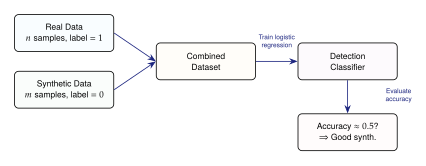
Machine Learning Utility: TSTR and Beyond
For many practitioners, the ultimate question is not whether the synthetic data looks statistically similar to the real data, but whether it is useful. Specifically: can we train a machine learning model on synthetic data and have it perform well on real data?
This question is formalised through the TSTR (Train on Synthetic, Test on Real) protocol:
Definition 43 (TSTR Protocol).
Given a real dataset split into and , and a synthetic dataset generated from :
Train a predictive model on .
Evaluate on .
Compare the performance to a model trained on and evaluated on .
The TSTR score is the ratio (or difference) between the performance of and : (TSTR) where is a suitable performance metric (accuracy, F1, AUC, RMSE, etc.). A TSTR score close to indicates that synthetic data is nearly as useful as real data for training.
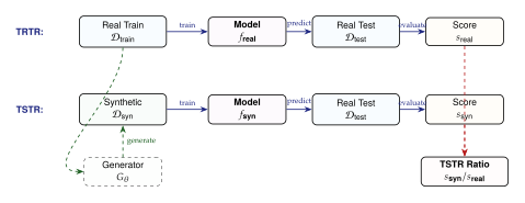
The TSTR protocol has several important variants:
TSTR with multiple models: to avoid bias from a single model choice, evaluate TSTR with several classifiers (logistic regression, random forest, XGBoost, neural network) and report the average or worst-case ratio.
TSTR with augmentation : train on a mixture of real and synthetic data, which often outperforms training on either alone. This measures whether synthetic data is useful as a complement to real data.
TRTS (Train on Real, Test on Synthetic) : the reverse protocol, which measures whether the synthetic data covers the same support as the real data. If TSTR is high but TRTS is low, the synthetic data may be “too easy” and missing important edge cases.
Caution.
TSTR scores depend heavily on the choice of downstream model and task. A synthetic dataset might achieve a TSTR ratio of for random forest classification but only for neural network regression on the same data. Always report TSTR across multiple models and tasks.
Exercise 53.
Suppose you have a binary classification dataset with positive class. A model trained on real data achieves accuracy on the test set. A model trained on synthetic data achieves accuracy.
Compute the TSTR ratio.
Is accuracy the right metric here? What would happen if simply predicted the majority class?
Argue that the TSTR ratio should be computed using a metric that accounts for class imbalance, such as AUC or balanced accuracy.
Detection Metrics
Detection metrics are the adversarial cousin of utility metrics. Instead of asking “is the synthetic data useful?” they ask “is the synthetic data detectable?” The underlying idea is simple: if a classifier can reliably distinguish real samples from synthetic samples, then the synthetic data has detectable artefacts.
The log-cluster metric from Definition 42 is one approach. TabStruct extends this idea with more sophisticated detection methods:
Algorithm 7.
Detection Score Computation
Label real samples as , synthetic samples as .
Split the combined dataset into training and test sets using stratified sampling.
Train a detection classifier (e.g., gradient-boosted decision tree) on the training set.
Evaluate on the test set using the AUROC (Area Under the Receiver Operating Characteristic curve).
The detection score is .
A detection score close to indicates high-quality synthetic data; a score close to indicates trivially detectable synthetic data.
An important subtlety is the choice of detection classifier. A simple logistic regression might miss complex artefacts that a gradient-boosted tree would catch. Conversely, an overly powerful classifier (e.g., a deep neural network) might overfit on irrelevant differences. TabStruct recommends using XGBoost with default hyperparameters as a reasonable middle ground.
Remark 37.
Detection metrics and GANs share a deep connection. The discriminator in a GAN is precisely a detection classifier that learns to distinguish real from generated samples. If we train a GAN to convergence, the discriminator achieves accuracy. Post-hoc detection metrics ask whether this equilibrium truly holds, or whether the discriminator was simply not powerful enough to find the remaining artefacts.
Privacy Metrics
The promise of synthetic data is not merely utility; it is privacy. The whole point of generating synthetic tables is often to share data without exposing individual records. But does generating synthetic data actually protect privacy? The answer is nuanced, and it depends critically on how we define and measure privacy.
TabStruct includes two families of privacy metrics: membership inference and attribute inference.
Membership Inference.
A membership inference attack asks: given a synthetic dataset and a target record , can we determine whether was in the training set used to generate the synthetic data? If the answer is yes, then the synthetic data is “memorising” aspects of the training data, which constitutes a privacy breach.
Formally, the attacker has access to the synthetic dataset and a target record . The attacker must output a binary decision: , where means the attacker believes was in the training set. The membership advantage is:
(MI Advantage)
An advantage of means the attacker is no better than random guessing; an advantage of means perfect inference. The most common attack strategy computes the distance from to its nearest neighbour in : records that were in the training set tend to have closer synthetic neighbours due to memorisation.
Attribute Inference.
Attribute inference is a stronger attack: given a synthetic dataset and a target record with one attribute hidden, can we infer the hidden attribute? This directly measures whether the synthetic data leaks individual-level information.
(AI Advantage)
where denotes all attributes except . The second term is the base rate: how well could we guess without any synthetic data, using only the other attributes? A positive advantage means the synthetic data provides additional information about individual records, which is a privacy concern.
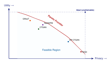
Key Idea.
There is a fundamental tension between utility and privacy in synthetic data generation. A synthetic dataset that perfectly reproduces the real distribution necessarily memorises all individual records. A synthetic dataset that reveals nothing about individuals is pure noise. The art lies in finding the right trade-off, and TabStruct's privacy metrics help quantify where a given method sits on this Pareto frontier.
The mathematical relationship between privacy and utility can be made precise through differential privacy:
Definition 44 (Differential Privacy for Synthetic Data).
A synthetic data generation mechanism satisfies -differential privacy if for all datasets , differing in exactly one record, and for all measurable sets of possible synthetic datasets: (DP) Smaller means stronger privacy. The parameter allows for a small probability of failure.
Differential privacy provides a worst-case guarantee. TabStruct's empirical privacy metrics (membership inference, attribute inference) provide average-case assessments that complement the formal guarantee. A method might satisfy -DP with a specific yet still show high membership inference advantage on certain datasets, particularly when the dataset has outliers that are easy to detect.
Exercise 54.
Consider two synthetic data generators: Generator A satisfies -differential privacy, while Generator B has no formal privacy guarantee but achieves a membership inference advantage of on all tested datasets.
Which generator would you trust more? Why?
Can a differentially private generator have high membership inference advantage? Under what circumstances?
Design an experiment to test whether a generator's empirical privacy matches its formal guarantee.
TabStruct's Structural Fidelity Score
TabStruct's key contribution is the structural fidelity score, which aggregates the hierarchical metrics into a single, interpretable number. The score is computed as a weighted combination:
(SFID)
where each component score with being best, is inverted because lower detection is better, and the weights satisfy . The default weights in TabStruct assign higher importance to pairwise and ML utility metrics, reflecting the insight that structural preservation matters more than marginal preservation.
Remark 38.
The specific weights are configurable, and TabStruct recommends choosing them based on the intended use case. For data augmentation, ML utility should be weighted highest. For statistical analysis, global utility and pairwise metrics matter most. For privacy-sensitive applications, the privacy component (not included in the basic structural fidelity score) should be added as an additional constraint rather than folded into the score.
Each component score is computed from the raw metrics via normalisation. For the column-wise score:
(SCOL)
For the pairwise score:
(Spair)
where is the normalised mutual information difference from (MI DIFF).
Insight.
TabStruct's hierarchical approach reveals a consistent empirical finding: methods that excel at column-wise metrics often underperform at pairwise metrics, and vice versa. For example, simple noise-addition methods achieve near-perfect marginal fidelity but destroy correlations. GAN-based methods often preserve correlations but distort marginals for rare categories. Diffusion-based methods tend to be more balanced across levels, which is one reason TabDDPM [6] has emerged as a strong baseline.
Worked Example: Applying TabStruct
Let us walk through a complete TabStruct evaluation on a toy example. Suppose we have a real dataset with samples and three columns:
: age (continuous, range )
: income bracket (categorical, low, medium, high)
: spending (continuous, range )
The real data has the following structure: older individuals tend to have higher income brackets, and higher income brackets are associated with higher spending. There is also a direct age–spending correlation.
We generate synthetic samples using two methods: Method A (a well-tuned CTGAN) and Method B (a simple method that independently samples each column from its marginal distribution).
Step 1: Column-wise Metrics.
| Metric | (age) | (income) | (spending) |
| KS (Method A) | 0.04 | – | 0.06 |
| KS (Method B) | 0.03 | – | 0.05 |
| TVD (Method A) | – | 0.05 | – |
| TVD (Method B) | – | 0.02 | – |
Step 2: Pairwise Metrics.
| Metric | |||
| (Method A) | 0.08 | 0.10 | 0.07 |
| (Method B) | 0.45 | 0.52 | 0.48 |
| (Method A) | 0.05 | 0.07 | 0.04 |
| (Method B) | 0.38 | 0.41 | 0.36 |
Step 3: Aggregate Scores.
| Method | ||||
| Method A (CTGAN) | 0.95 | 0.87 | 0.83 | 0.88 |
| Method B (Marginal) | 0.97 | 0.38 | 0.41 | 0.55 |
Insight.
Method B wins on column-wise metrics but loses catastrophically overall. This is precisely the scenario that TabStruct was designed to catch. Any evaluation that considers only marginal fidelity would incorrectly conclude that Method B is superior.
Exercise 55.
Extend the above example by adding a fourth column that is a deterministic function of and (e.g., ). Describe what additional pairwise and higher-order structure this introduces, and explain why pairwise metrics alone might still miss the three-way dependency between , , and .
Evaluation Frameworks and Metrics for Synthetic Data
TabStruct gave us a hierarchical way to think about evaluation. But evaluation in practice requires more than a set of metrics: it requires frameworks, libraries, benchmarks, and protocols that make evaluation reproducible, standardised, and fair. In this section, we broaden our scope from TabStruct's specific contributions to the entire landscape of synthetic data evaluation.
We will cover standardised libraries, statistical tests, information-theoretic metrics, downstream evaluation, fairness, and comprehensive benchmarking protocols. By the end, you will have a complete toolkit for evaluating any synthetic data generator, along with a clear understanding of which metrics to use in which situations.
SDMetrics and Standardised Evaluation
The Synthetic Data Vault (SDV) project, led by researchers at MIT, introduced SDMetrics as an open-source library for evaluating synthetic data. SDMetrics provides a standardised API for computing a wide range of quality metrics, organised into three categories:
Column Shapes: measures how well the synthetic data preserves the shape (distribution) of each individual column.
Column Pair Trends: measures how well the synthetic data preserves the relationships between pairs of columns.
New Row Synthesis: measures whether the synthetic rows are genuinely new (not copies of real rows), addressing both novelty and privacy.
Each category produces a score between and , and the overall quality score is the average of these three categories.
Algorithm 8.
SDMetrics Quality Evaluation Protocol
Load real data and synthetic data .
For each column : enumerate
If continuous: compute KS complement .
If categorical: compute TVD complement . enumerate
For each column pair : enumerate
If both continuous: compute correlation similarity .
If both categorical: compute contingency similarity.
If mixed: compute category-conditional KS complement. enumerate
Compute nearest-neighbour distance ratio for new row synthesis.
Report per-metric scores and overall quality score.
Remark 39.
SDMetrics intentionally uses simple, interpretable metrics rather than complex ones. The philosophy is that practitioners need metrics they can understand and explain to stakeholders. The KS statistic, for example, has a clear interpretation: it is the maximum vertical distance between two CDFs. More sophisticated metrics like MMD or Wasserstein distance, while theoretically superior, are harder to explain to a non-technical audience.
Statistical Tests for Distribution Comparison
Beyond point metrics, we often want to perform formal hypothesis tests: is there statistically significant evidence that the real and synthetic distributions differ? This question calls for classical statistical machinery.
The Kolmogorov–Smirnov Test.
We have already seen the KS statistic (Definition 38). The associated KS test provides a -value under the null hypothesis . Under , the scaled statistic converges to the Kolmogorov distribution.
Proposition 17 (KS Test Consistency).
The two-sample KS test is consistent: for any alternative hypothesis , the power of the test converges to as the sample sizes .
The KS test is distribution-free (it requires no parametric assumptions) and is applicable to any continuous column. For categorical columns, we use the chi-squared test instead.
The Chi-Squared Test.
For a categorical column with categories, the chi-squared statistic compares observed and expected frequencies:
(Chisq)
where is the observed frequency of category in the synthetic data and is the expected frequency based on the real data. Under , this statistic follows a chi-squared distribution with degrees of freedom.
For comparing joint distributions of two categorical columns, we use the chi-squared test of independence on the contingency table.
The Anderson–Darling Test.
The Anderson–Darling (AD) test is a refinement of the KS test that gives more weight to the tails of the distribution:
(AD)
where are the order statistics and is the reference CDF. The AD test is particularly useful for tabular data because tail behaviour often matters: rare events (outliers, edge cases) are precisely the cases where synthetic data tends to fail.
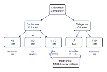
Caution.
With large sample sizes (which are common in tabular data), virtually any statistical test will reject . Even tiny, practically insignificant differences become statistically significant. Always complement hypothesis tests with effect size measures (the actual KS statistic, TVD, or MMD value) and interpret them in context.
Information-Theoretic Metrics
Information theory provides a principled framework for measuring the distance between distributions. The two most important metrics for synthetic data evaluation are the Kullback–Leibler (KL) divergence and mutual information preservation.
KL Divergence.
The KL divergence from the real distribution to the synthetic distribution is:
(KL)
For discrete distributions:
(KL Discrete)
The KL divergence is non-negative and equals zero if and only if . However, it is asymmetric: in general. This asymmetry has practical implications.
Key Idea.
penalises the synthetic distribution for failing to cover regions where the real distribution has mass (mode dropping). penalises the synthetic distribution for placing mass where the real distribution has none (hallucination). Both failure modes matter for synthetic data; using the symmetrised version (Jensen–Shannon divergence) or reporting both directions is advisable.
The Jensen–Shannon (JS) divergence symmetrises the KL divergence:
(JS)
The JS divergence is symmetric, bounded ( when using natural logarithm), and always well-defined even when and have different support.
Mutual Information Preservation.
Beyond comparing marginal distributions, we want to know whether the synthetic data preserves the dependency structure of the real data. This is captured by the mutual information matrix:
(MI Matrix)
The mutual information preservation score is:
(MI PRES)
where we normalise by joint entropy to obtain a value in .
Remark 40.
Estimating mutual information from finite samples is notoriously difficult, particularly in high dimensions. The most common approach for continuous variables discretises them into bins and computes the discrete mutual information. More sophisticated approaches use -nearest-neighbour estimators (the Kraskov– Stögbauer–Grassberger estimator), which are consistent but can have high variance for small samples.
The Wasserstein Distance.
The Wasserstein distance (also called the earth mover's distance) provides yet another way to compare distributions, with the advantage of being sensitive to the geometry of the sample space:
Definition 45 (Wasserstein-1 Distance).
The Wasserstein-1 distance between distributions and on a metric space is: (Wasserstein) where is the set of all joint distributions (couplings) with marginals and .
For one-dimensional distributions, the Wasserstein-1 distance has a closed-form expression in terms of the CDFs:
(Wasserstein 1D)
Insight.
The Wasserstein distance is related to, but distinct from, the KS statistic. The KS statistic measures the maximum absolute difference between CDFs; the Wasserstein distance measures the integral of the absolute difference. The Wasserstein distance is more informative because it accounts for the magnitude of discrepancies everywhere, not just at the worst point.
Benchmarking Protocols
Individual metrics, however well-chosen, are only as useful as the benchmarking protocol in which they are embedded. A rigorous benchmark must specify:
Datasets: which real datasets are used, how they are pre-processed, and how train/test splits are created.
Baselines: which methods are compared, with what hyperparameters, and whether the hyperparameters were tuned on a validation set.
Metrics: which metrics are reported, at which levels of the evaluation hierarchy, and how they are aggregated.
Repetitions: how many random seeds are used, and whether confidence intervals are reported.
Compute: what hardware was used and how long each method was trained.
Standard Benchmark Datasets.
The tabular data generation community has converged on a small set of benchmark datasets, each chosen to test different aspects of generation quality:
| Dataset | Domain | Rows | Cont. | Cat. |
| Adult Income | Census | 48,842 | 6 | 8 |
| Covertype | Forest | 581,012 | 10 | 44 |
| Intrusion | Network | 494,021 | 34 | 7 |
| Credit | Finance | 284,807 | 30 | 1 |
| Loan | Finance | 9,578 | 6 | 7 |
| News | Media | 39,797 | 59 | 2 |
| King County | Real estate | 21,613 | 17 | 4 |
| California | Housing | 20,640 | 8 | 0 |
Caution.
Over-reliance on a small set of benchmark datasets creates the risk of overfitting the community's methods to those specific datasets. A method that achieves state-of-the-art on Adult and Covertype may fail on a novel dataset with different characteristics (e.g., high cardinality categorical columns, extreme class imbalance, or temporal dependencies). Always supplement standard benchmarks with domain-specific datasets relevant to your application.
The Benchmarking Pipeline.
A well-designed benchmark follows a standardised pipeline, which we illustrate in Figure 49.
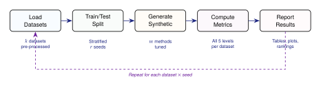
Downstream Task Evaluation
Statistical similarity is a necessary condition for good synthetic data, but it is not sufficient. The ultimate test is performance on downstream tasks: the actual analyses and models that practitioners intend to build with the data.
Classification and Regression.
The TSTR protocol from Machine Learning Utility: TSTR and Beyond is the standard approach for classification and regression tasks. To make the evaluation robust, we recommend:
Use at least three diverse classifiers/regressors: logistic regression (linear baseline), random forest (tree-based), and a neural network (deep learning).
Report both the absolute performance on the synthetic-trained model and the TSTR ratio relative to the real-trained model.
Use stratified cross-validation rather than a single train/test split.
For imbalanced datasets, use metrics that are robust to class imbalance (AUC-ROC, F1, balanced accuracy) rather than simple accuracy.
Clustering.
For unsupervised tasks, we can evaluate whether the synthetic data preserves cluster structure. The protocol is:
Apply a clustering algorithm (e.g., -means) to both the real and synthetic data separately.
Compare the cluster centres, sizes, and assignments using the Adjusted Rand Index (ARI) or Normalised Mutual Information (NMI).
A high ARI between real and synthetic clusterings indicates that the global structure is preserved.
Feature Importance Preservation.
Another important downstream metric is whether the synthetic data preserves the relative importance of features. If a random forest trained on real data identifies features , , (in that order) as most important for predicting the target, and a random forest trained on synthetic data identifies the same ranking, then the synthetic data preserves the signal structure.
(FI PRES)
where and are the feature importance rankings and is Kendall's tau distance.
Fairness Evaluation of Synthetic Data
Synthetic data is sometimes proposed as a tool for debiasing: generating data that is more balanced or fair than the original. Conversely, a poorly designed generator might amplify biases present in the training data. Fairness evaluation is therefore essential.
The Fairness Challenge.
Consider a dataset used to train a loan approval model. The real data contains historical biases: applicants from certain demographic groups are approved at lower rates, even after controlling for creditworthiness. If we generate synthetic data from this biased dataset, the synthetic data will inherit (and potentially amplify) these biases.
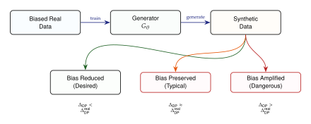
The key fairness metrics for synthetic data evaluation are:
Definition 46 (Demographic Parity Gap).
Let be a sensitive attribute (e.g., race, gender) and be a binary outcome. The demographic parity gap is: (DP GAP) A of indicates perfect demographic parity.
Definition 47 (Equalised Odds Gap).
The equalised odds gap measures the maximum difference in true positive rates and false positive rates across groups: (EO GAP)
For synthetic data evaluation, we compute these gaps on both the real and synthetic data and compare:
(Fairness Change)
A negative indicates the synthetic data has reduced bias (good for debiasing applications); a positive value indicates amplification (a red flag).
Exercise 56.
A real dataset has and , giving . Three generators produce synthetic data with:
Generator 1: , .
Generator 2: , .
Generator 3: , .
Compute and for each. Which generator reduces bias? Which amplifies it? Is Generator 2 always desirable? (Hint: consider whether perfect demographic parity might destroy legitimate correlations in the data.)
Comprehensive Method Comparison
With our evaluation toolkit in hand, we can now present a comprehensive comparison of the methods covered in this chapter. The following tables summarise results across multiple benchmark datasets, using the TabStruct evaluation hierarchy.
Overall Quality Scores.
Remark 41.
These scores represent averages across multiple benchmark datasets and should be interpreted as rough guidelines, not absolute rankings. Performance varies significantly across datasets: CTGAN excels on datasets with many categorical columns, while TabDDPM is strongest on datasets with complex continuous distributions. No single method dominates across all datasets and all metrics.
TSTR Results by Downstream Model.
| Method | LR | RF | XGB | MLP |
| CTGAN | 0.92 | 0.87 | 0.89 | 0.84 |
| CTAB-GAN+ | 0.93 | 0.90 | 0.91 | 0.87 |
| TabDDPM | 0.96 | 0.93 | 0.94 | 0.91 |
| GReaT | 0.94 | 0.91 | 0.92 | 0.88 |
| TabuLa | 0.91 | 0.88 | 0.90 | 0.85 |
The columns are: LR = Logistic Regression, RF = Random Forest, XGB = XGBoost, MLP = Multi-Layer Perceptron. Each value is the TSTR ratio (higher is better, is perfect).
Privacy–Utility Trade-off.
| Method | MI Advantage | AI Advantage | TSTR (XGB) |
| CTGAN | 0.08 | 0.05 | 0.89 |
| CTAB-GAN+ | 0.07 | 0.04 | 0.91 |
| TabDDPM | 0.05 | 0.03 | 0.94 |
| GReaT | 0.12 | 0.09 | 0.92 |
| TabuLa | 0.15 | 0.11 | 0.90 |
Insight.
LLM-based methods (GReaT, TabuLa) tend to have higher privacy risk than GAN or diffusion-based methods. This is likely because language models have large memory capacity and are prone to memorising training sequences. If privacy is a primary concern, diffusion-based methods or GAN-based methods with differential privacy are preferable.
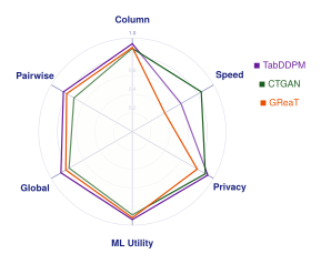
When to Use Which Method.
The comparison results suggest the following practical guidelines:
Default choice: TabDDPM offers the best overall quality and is a strong default for most applications.
Privacy-sensitive applications: Use CTGAN or CTAB-GAN+ with differential privacy, or TabDDPM with DP-SGD. LLM-based methods should be used cautiously when privacy matters.
Small datasets: LLM-based methods (GReaT, TabuLa) excel on small datasets because they leverage pre-trained knowledge. When the real dataset has fewer than 1,000 rows, LLM-based methods often outperform purpose-built architectures.
High-cardinality categorical columns: CTGAN and CTAB-GAN+ handle high-cardinality categories more gracefully than diffusion-based methods.
Speed constraints: CTGAN and TVAE are the fastest methods. TabDDPM and LLM-based methods are significantly slower.
Building a Complete Evaluation Report
We conclude this section by outlining how to build a complete evaluation report for a synthetic data generator. A thorough report should include all five levels of the TabStruct hierarchy, plus additional context.
Algorithm 9.
Complete Evaluation Report Protocol
Data Description: summarise the real dataset (number of rows, columns, types, class balance, missing values).
Level 1 – Column-wise: report KS/TVD for each column, plus histograms comparing real and synthetic distributions for the most important columns.
Level 2 – Pairwise: report the correlation matrix difference, mutual information difference, and conditional distribution distances. Include heatmaps of the correlation matrices.
Level 3 – Global: report MMD, log-cluster metric, and principal component analysis (PCA) projections showing overlap between real and synthetic data.
Level 4 – ML Utility: report TSTR ratios for at least three downstream models and at least two metrics (e.g., AUC and F1).
Level 5 – Privacy: report membership inference advantage and attribute inference advantage. If differential privacy is claimed, state the parameters and verify empirically.
Fairness: if the data contains sensitive attributes, report demographic parity and equalised odds gaps, comparing real and synthetic data.
Computational Cost: report training time, sampling time, and hardware requirements.
Exercise 57.
You are given a healthcare dataset with rows, continuous columns, categorical columns, and a binary target (disease/no disease). One categorical column is a sensitive attribute (ethnicity). Design a complete evaluation protocol using the framework above. For each level, specify:
The exact metrics you will compute.
The statistical tests you will perform.
The visualisations you will produce.
Any domain-specific considerations (e.g., medical plausibility checks).
Causal Structure Preservation
A frontier topic in synthetic data evaluation is whether the generated data preserves the causal structure of the real data, not merely its statistical associations. Two datasets can have identical joint distributions yet encode entirely different causal mechanisms. If the real data satisfies (income causes spending) but the synthetic data is generated in a way that reverses the causal direction, then interventional queries on the synthetic data will yield incorrect answers.
Definition 48 (Structural Hamming Distance).
Let and be directed acyclic graphs (DAGs) estimated from the real and synthetic data, respectively. The Structural Hamming Distance (SHD) is the number of edge additions, deletions, and reversals needed to transform into .
In practice, we estimate causal graphs from both datasets using a structure learning algorithm (e.g., the PC algorithm or GES) and compare them using the SHD. A low SHD indicates that the synthetic data preserves causal relationships.
(Causal Score)
where for variables (the maximum possible SHD in a DAG with nodes).
Remark 42.
Causal discovery from observational data is itself an unsolved problem, so the estimated graphs and may both be incorrect. The comparison measures consistency between the two estimates rather than absolute correctness. When a known causal graph is available (e.g., from domain expertise), it should be used as the reference instead of the data-estimated graph.
Exercise 58.
Consider a dataset with three variables: (education level), (income), and (spending), where the true causal graph is . A synthetic data generator produces data where the marginals and pairwise correlations are preserved, but the conditional independence structure is violated: in the synthetic data, (i.e., there is a direct effect of education on spending even after controlling for income).
What is the SHD between the true graph and the graph implied by the synthetic data?
Would standard pairwise metrics detect this discrepancy? Why or why not?
Design a statistical test based on conditional independence that could detect this specific failure mode.
Scalability and Computational Considerations
Evaluation itself can be computationally expensive. For a dataset with columns, computing all pairwise metrics requires comparisons. Each comparison may involve sorting ( for the KS statistic) or kernel evaluations ( for MMD). For large datasets with many columns, the evaluation cost can rival or exceed the generation cost.
| Metric | Per-Comparison | Total ( cols) |
| KS Statistic | ||
| TVD | ||
| Correlation Matrix | ||
| MMD | ||
| TSTR (one model) | ||
| MI Estimation (KSG) | ||
| Detection Score |
For practitioners working with large-scale datasets (hundreds of thousands of rows, dozens of columns), a staged evaluation strategy is recommended:
Quick check: compute column-wise metrics (fast, ) to catch gross failures.
Medium check: add pairwise correlation comparison () and the log-cluster detection metric.
Full evaluation: compute MMD, TSTR across multiple models, privacy metrics, and fairness analysis. This is expensive but necessary for publication or deployment.
Insight.
A staged evaluation strategy saves significant computation while still catching most quality issues early. In practice, if a generator fails at Level 1 (column-wise metrics), there is no need to proceed to more expensive evaluations. Fix the generator first, then re-evaluate.
Open Challenges in Evaluation
Despite the progress represented by TabStruct and SDMetrics, several fundamental challenges remain.
Higher-Order Dependencies.
All the metrics we have discussed capture at most pairwise relationships. Real data often contains three-way, four-way, or even higher-order dependencies. For example, the interaction between age, diagnosis, and treatment cost in a medical dataset cannot be fully captured by any combination of pairwise metrics. Developing scalable metrics for higher-order fidelity is an open problem.
Temporal and Sequential Structure.
When tabular data has a temporal component (e.g., patient records over time), evaluation must also assess whether the synthetic data preserves temporal patterns: trends, seasonality, and auto- correlations. Standard TabStruct metrics do not address this.
Domain-Specific Validity.
A synthetic medical record might pass every statistical test yet contain clinically impossible combinations (e.g., a 5-year-old patient with a diagnosis of age-related macular degeneration). Domain-specific validity checks require expert knowledge and are difficult to automate.
The Curse of Dimensionality.
As the number of columns increases, the number of pairwise comparisons grows quadratically, and the difficulty of estimating joint distributions grows exponentially. For high-dimensional tables (50+ columns), current metrics may fail to detect subtle but important structural failures.
Key Idea.
Evaluation of synthetic tabular data is not a solved problem. TabStruct and SDMetrics represent important steps, but the field needs better metrics for higher-order structure, temporal dependencies, domain validity, and high-dimensional settings. The evaluation problem may, in the end, be harder than the generation problem itself.
Exercise 59.
Propose a metric for three-way dependency preservation. (Hint: consider the interaction information, a generalisation of mutual information to three variables.)
Design an evaluation protocol for a synthetic dataset with temporal structure (e.g., daily stock prices with 20 features). What additional metrics would you need beyond TabStruct?
A synthetic dataset passes all TabStruct metrics with scores above but contains of rows that violate known domain constraints (e.g., negative ages, future dates). How would you modify the evaluation framework to catch this?
Challenge 6.
The “evaluation meta-problem”: define a metric for evaluating evaluation metrics. Given two metrics and for synthetic data quality, how would you determine which metric is more informative? (Hint: consider the metric's ability to predict downstream task performance, its sensitivity to known defects, and its robustness to dataset characteristics.)
GFlowNets for Structured Generation
Every generative model we have studied so far shares a common strategy: learn a single distribution over the data space, then sample from it. GANs learn a generator that maps noise to data. Diffusion models learn a reverse process that denoises. Autoregressive models learn to predict the next token. In each case, the goal is to produce samples that look like the training data, and the training signal comes from matching the model's output distribution to the empirical distribution of observed examples.
But what if the goal is not to imitate a dataset, but to discover new objects that score highly under a given reward function? What if we want not the single best object, but a diverse set of high-quality objects? What if the objects are combinatorial structures, molecules, graphs, or discrete sequences, and the reward landscape is rugged, multimodal, and expensive to evaluate?
This is the setting that Generative Flow Networks, or GFlowNets, were designed to address. Introduced by Yoshua Bengio and collaborators in 2021 [55], and refined in a series of subsequent papers [56][57], GFlowNets represent a fundamentally different approach to generative modelling. They do not learn to imitate data. They learn to sample in proportion to a reward.
The distinction is profound. A GAN trained on molecules will generate molecules that resemble the training set. A GFlowNet trained with a reward function that measures drug-likeness will generate a diverse collection of molecules, each with high drug-likeness, including molecules that look nothing like any training example. This is not reinforcement learning (which seeks the single highest-reward object) and it is not density estimation (which seeks to match an observed distribution). It is something new: proportional sampling from a reward function over a combinatorial space.
Key Idea.
GFlowNets sample composite objects with probability proportional to a reward function . Unlike reinforcement learning, which concentrates probability on the single best action sequence, GFlowNets maintain diversity by sampling proportionally: objects with twice the reward are sampled twice as often, but low-reward objects are not eliminated entirely. This makes GFlowNets ideal for exploring multimodal reward landscapes where diversity matters.
The DAG Formulation: States, Actions, and Flows
The central mathematical object in GFlowNet theory is a directed acyclic graph (DAG) that describes how composite objects are constructed step by step. Let us build this formalism carefully.
Definition 49 (GFlowNet State Space).
A GFlowNet state space is a tuple where:
is a finite set of states, representing partially constructed objects;
is a set of actions (directed edges), where means that state can transition to state by adding one component;
is the unique initial state (the empty object);
is the set of terminal states (completed objects).
The pair must form a directed acyclic graph with as the unique source. Every terminal state must be reachable from .
The intuition is simple. Think of building a molecule atom by atom. The initial state is the empty molecule. Each action adds an atom or a bond. Non-terminal states are partially assembled molecules. Terminal states are complete molecules ready for evaluation. The DAG structure ensures that construction is irreversible: once you add an atom, you cannot remove it (though the same complete molecule may be reachable via different construction orders).
Example 21.
Consider generating binary strings of length 3. The state space consists of all prefixes: the empty string , the strings and , the strings , , , , and the terminal strings , , , , , , , . Each non-terminal state has exactly two outgoing actions (append 0 or append 1). The DAG has states and edges. A trajectory from to a terminal state corresponds to a specific order of bit choices.
Now we introduce the key concept: flow.
Definition 50 (Flow Function).
A flow function on is a non-negative function that assigns a flow to each edge. The state flow is defined as where the first sum is over incoming edges and the second is over outgoing edges. This equality is the flow conservation condition: at every non-terminal, non-initial state, the total incoming flow equals the total outgoing flow.
The analogy to fluid dynamics is intentional. Imagine water flowing through a network of pipes. Water enters at the source , flows through the DAG along edges, and exits at terminal states. The amount of water exiting at each terminal state is . If we normalize by the total flow , then gives a probability distribution over terminal states.
The fundamental insight of GFlowNets is this: if we choose the flow function so that for all terminal states , then the resulting distribution samples proportionally to the reward: (Gflownet Sampling)
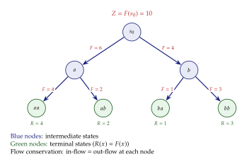
Flow Matching and the Detailed Balance Condition
The elegant picture of Figure 52 raises an immediate practical question: how do we learn the flow function? We cannot simply set at terminal states and work backwards, because the number of paths through the DAG grows combinatorially with the object size. We need a trainable parametric model and a loss function.
The original GFlowNet paper [55] proposed the flow matching condition as the basis for training.
Definition 51 (Flow Matching Condition).
A parameterized flow satisfies the flow matching condition if, for every non-terminal state , (FLOW Matching) For the initial state , the incoming flow is defined as (a learnable scalar), and for terminal states, the outgoing “flow” is the reward .
The flow matching loss penalizes violations of this condition: (FLOW Matching LOSS) where is a distribution over non-terminal states used for training (typically a mixture of on-policy and off-policy samples). The use of log-space is crucial: it prevents numerical issues when flows span many orders of magnitude, which they typically do in combinatorial spaces.
However, flow matching has a significant limitation. It requires summing over all parents and children of every state visited during training. For states with many parents (which arise when the same partial object can be reached by many construction orders), this sum is expensive. This motivated the detailed balance condition.
Definition 52 (Detailed Balance Condition).
A parameterized flow satisfies the detailed balance condition if, for every edge , (Detailed Balance) where is the forward policy and is the backward policy. For terminal states , we set .
The detailed balance condition is a local condition on individual edges, not a global condition on states. This makes it cheaper to evaluate but also more restrictive: detailed balance implies flow matching, but not vice versa. Nevertheless, detailed balance is often preferred in practice because it avoids the expensive summation over parents and children.
Insight.
The relationship between flow matching and detailed balance mirrors a classic distinction in statistical physics. In a Markov chain at equilibrium, global balance (the total probability flowing into each state equals the total probability flowing out) is necessary and sufficient for stationarity. Detailed balance (balance holds for each pair of states individually) is a stronger condition that implies global balance. GFlowNets inherit this hierarchy: flow matching is global balance, and the detailed balance condition is its stricter cousin.
Training: Trajectory Balance and Sub-Trajectory Balance
The most important training objective for GFlowNets, and the one used in most practical implementations, is the trajectory balance (TB) loss introduced by Malkin et al. [57]. The key insight is beautiful in its simplicity: instead of enforcing balance at individual edges or states, enforce it over entire trajectories from to a terminal state.
Definition 53 (Trajectory Balance).
Let be a complete trajectory from the initial state to a terminal state . The trajectory balance condition states that (Trajectory Balance) where is the learnable partition function, is the forward policy, and is the backward policy.
The trajectory balance loss takes the log ratio and penalizes its squared deviation from zero: (TB LOSS)
Remark 43.
The trajectory balance condition is both necessary and sufficient for the GFlowNet to sample proportionally to the reward. If the TB condition holds for all trajectories, then for all terminal states . Conversely, if the GFlowNet samples proportionally to the reward and the backward policy is correct, then the TB condition holds. This makes it a tighter training objective than flow matching or detailed balance alone.
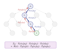
A further refinement is the sub-trajectory balance (SubTB) condition [57], which enforces balance over sub-paths rather than complete trajectories. This provides denser training signal and faster credit assignment.
Definition 54 (Sub-Trajectory Balance).
For any sub-trajectory within a complete trajectory , the sub-trajectory balance condition requires (Subtb) where is the learnable state flow for intermediate states, and for terminal states .
The SubTB loss sums the squared log-ratio over all sub-trajectories (or a random subset) within each sampled trajectory: (Subtb LOSS) where is a weighting parameter that downweights longer sub-trajectories.
Remark 44.
The hierarchy of GFlowNet training objectives forms a neat spectrum. At one extreme, detailed balance enforces balance on individual edges (sub-trajectories of length 1). At the other extreme, trajectory balance enforces balance on complete paths. Sub-trajectory balance interpolates between these extremes. In practice, trajectory balance is the most commonly used objective because it requires the fewest parameterized quantities (just , , and ), while sub-trajectory balance offers faster convergence at the cost of also learning state flows .
Connection to MCMC and Variational Inference
GFlowNets did not emerge in a vacuum. They connect deeply to two pillars of probabilistic computation: Markov chain Monte Carlo (MCMC) and variational inference (VI). Understanding these connections illuminates why GFlowNets work and where they fit in the broader landscape.
Connection to MCMC.
Both MCMC and GFlowNets aim to sample from a distribution proportional to a reward (or unnormalized density). MCMC does this by constructing a Markov chain whose stationary distribution is the target. The chain starts from an arbitrary state and, after a burn-in period, produces correlated samples from the target.
GFlowNets take a fundamentally different approach: they learn a constructive policy that builds objects from scratch. Each sample is independent (no Markov chain, no burn-in, no mixing time). The price is that the policy must be trained, which requires many reward evaluations during training. The benefit is that, once trained, sampling is fast and embarrassingly parallel.
Proposition 18 (GFlowNet as Amortized MCMC).
Let be the target distribution. An MCMC sampler produces a sequence of dependent samples that converge to as the chain length grows. A trained GFlowNet produces independent samples from , where the approximation quality depends on the training loss. In this sense, a GFlowNet can be viewed as an amortized MCMC sampler: the computational cost of mixing is paid once during training, and at test time, each sample is drawn in a single forward pass.
Connection to variational inference.
Variational inference posits a family of distributions and minimizes , where . A GFlowNet's forward policy defines a distribution over terminal states . When the trajectory balance loss is minimized, , which is exactly the target. Thus, GFlowNet training can be interpreted as a form of variational inference where the variational family is the set of all constructive policies on the DAG.
Theorem 8 (TB Loss as Variance of Log-Ratio).
The trajectory balance loss equals the variance (under the training distribution ) of the log-ratio between the forward and backward trajectory probabilities. When , the log-ratio is constant across all trajectories, which implies for all terminal states . Moreover, the optimal value of equals , providing a free estimate of the partition function.
Proof.
Let denote the log-ratio for trajectory . The TB loss is . When this loss is zero, for all trajectories in the support of . Exponentiating and summing over all trajectories terminating at , we obtain for all , hence . Summing over all gives .
Why GFlowNets Matter for Structured Data
The connection between GFlowNets and structured data generation is both natural and powerful. Structured objects, whether molecules, graphs, programs, or combinatorial configurations, are typically built step by step. A molecule is assembled atom by atom. A graph grows edge by edge. A program is written token by token. This sequential construction is exactly what the GFlowNet DAG captures.
Moreover, structured data problems often come with a reward function rather than a dataset. In drug discovery, the reward might be a combination of binding affinity, synthetic accessibility, and drug-likeness. In combinatorial optimization, the reward is the objective function. In Bayesian structure learning, the reward is the posterior probability of a graph given data. GFlowNets are tailor-made for these settings.
Example 22.
Consider generating drug-like molecules with high binding affinity to a target protein. The state space consists of partially assembled molecular graphs. Actions add atoms (C, N, O, S, etc.) or bonds (single, double, triple) to the growing molecule. The reward is the exponentiated binding affinity predicted by a docking program or a learned proxy. A GFlowNet trained on this reward will generate diverse molecules with high binding affinity, exploring multiple scaffolds and functional groups rather than collapsing to a single optimum.
Example 23.
In Bayesian structure learning, the goal is to infer the structure of a Bayesian network (a directed acyclic graph) from observational data. The reward function is the marginal likelihood , and the GFlowNet samples DAGs with probability proportional to their posterior probability. This is particularly valuable because the space of DAGs over nodes grows super-exponentially (), making exhaustive enumeration impossible for even moderate . A GFlowNet can explore this space efficiently, producing a diverse posterior sample that captures uncertainty about the true structure.
Combinatorial optimization.
GFlowNets also connect to combinatorial optimization through the temperature parameter. If the reward is , then as , the sampling distribution concentrates on the global optimum. At moderate , the GFlowNet explores a neighborhood of high-quality solutions. This allows practitioners to trade off between exploitation (high , finding the best solution) and exploration (low , finding diverse good solutions).
Algorithm 10: GFlowNet Training with Trajectory Balance.
- Input: Reward function ; forward policy ; backward policy ; learnable partition function ; exploration parameter
- Initialize , , randomly
- for iteration
- Sample trajectory: starting from , at each state , sample
- Continue until reaching a terminal state
- Record trajectory
- Compute reward
- Compute TB loss:
- Update by gradient descent on
- Output: Trained forward policy
Applications of GFlowNets
Since their introduction, GFlowNets have been applied to a growing list of structured generation problems. We highlight three representative applications.
Molecule generation.
The original GFlowNet paper demonstrated the approach on molecule generation, building molecules as graphs where nodes are atoms and edges are bonds. The action space includes adding atoms of various types and forming bonds between existing atoms. Using a reward based on a proxy model of binding affinity, the GFlowNet generates diverse molecules that are both novel and high-scoring. Compared to reinforcement learning baselines (which collapse to a single high-reward molecule and minor variants), GFlowNets produce orders of magnitude more unique molecules while maintaining comparable reward quality.
Bayesian structure learning.
Deleu et al. applied GFlowNets to the problem of sampling directed acyclic graphs from the posterior distribution given data [56]. The state space consists of partially constructed DAGs, and actions add directed edges. The acyclicity constraint is enforced by only allowing edges that do not create cycles. The reward is the marginal likelihood, which can be computed in closed form for linear Gaussian models. The GFlowNet posterior approximation matches or exceeds variational inference baselines while producing more diverse graph samples.
Biological sequence design.
GFlowNets have been applied to the design of DNA aptamers, RNA sequences, and antimicrobial peptides. In each case, the state space is the set of all prefixes of a biological sequence, actions append nucleotides or amino acids, and the reward reflects biological activity predicted by a learned oracle. The diversity of GFlowNet samples is particularly valuable in biological design, where synthesizing and testing multiple diverse candidates increases the probability of finding a successful drug or diagnostic tool.
Exercise 60.
Consider a GFlowNet for generating binary strings of length 4, with reward where is the number of 1s in .
Compute the partition function .
What is the probability of sampling the string ?
What is the probability of sampling any string with exactly two 1s?
Write out the trajectory balance condition for the trajectory .
Exercise 61.
Prove that the detailed balance condition (Definition 52) implies the flow matching condition (Definition 51). Show by explicit counterexample that the converse does not hold. Hint: Sum the detailed balance equation over all children of a state .
Advanced Topics: Consistency Models, Uncertainty, and Beyond
The structured data generation landscape continues to evolve rapidly. In this section, we survey several advanced topics that push the boundaries of what is possible: consistency models adapted for tabular data, uncertainty quantification for synthetic data, conformal prediction guarantees, active learning strategies, and federated approaches to synthetic data generation. Each topic addresses a fundamental limitation of the methods we have studied so far, and each opens new avenues for research and application.
Consistency Models for Tabular Data
Diffusion models have proven remarkably effective for tabular data, as we saw with TabDDPM and its successors. However, they share a fundamental limitation with all iterative denoising approaches: sampling requires many sequential denoising steps, making generation slow. For applications that demand real-time synthetic data, such as online data augmentation during training or interactive data exploration tools, this latency is unacceptable.
Consistency models, introduced by Song et al. [58], offer an elegant solution. The key idea is to learn a function that maps any point on the diffusion trajectory directly to the clean data point, enabling one-step generation without iterative denoising.
Definition 55 (Consistency Function).
Let be a diffusion trajectory governed by the probability flow ODE where is the drift function derived from the score. A consistency function satisfies the self-consistency property: (Consistency) In particular, for all , meaning that the consistency function recovers the clean data point from any noise level.
Adapting to tabular data.
The adaptation of consistency models to tabular data requires handling the same challenges that arose in TabDDPM: mixed data types, multimodal continuous distributions, and categorical variables. The approach combines the hybrid forward process (Gaussian noise for continuous columns, multinomial diffusion for categorical columns) with a consistency distillation procedure.
Algorithm 11: Consistency Distillation for Tabular Data.
- Input: Pre-trained tabular diffusion model ; consistency model ; EMA rate ; time schedule
- Initialize and target network with
- for iteration
- Sample ,
- Compute noisy sample using hybrid forward process
- Compute one-step denoised estimate
- Compute distillation loss: where is a distance metric (e.g., Huber loss for continuous, cross-entropy for categorical)
- Update by gradient descent on
- Update target:
- Output: Consistency model
The practical benefits are substantial. Empirical evaluations on standard tabular benchmarks (Adult, Default of Credit, Covertype) show that consistency-distilled tabular models achieve 95% or more of the quality of the original diffusion model while reducing generation time by 10–50. For a table with one million rows, this can reduce generation time from hours to minutes.
Remark 45.
Consistency models also support a multi-step generation mode, where 2–4 denoising steps are used instead of one. This provides a smooth quality-speed tradeoff: more steps yield higher quality at the cost of proportionally more computation. For tabular data, 2 steps often suffice to close the remaining gap with the full diffusion model.
Uncertainty Quantification in Synthetic Data
When we replace real data with synthetic data, a natural question arises: how much can we trust the synthetic data? If a classifier trained on synthetic data makes a prediction, how confident should we be in that prediction? If a statistical analysis reveals a correlation in synthetic data, does that correlation exist in the real population, or is it an artefact of the generative model?
These questions fall under the umbrella of uncertainty quantification (UQ) for synthetic data, a topic that is critical for high-stakes applications but has received surprisingly little attention until recently.
Sources of uncertainty.
There are three distinct sources of uncertainty when working with synthetic data:
Aleatoric uncertainty: inherent randomness in the data-generating process. Even with a perfect generative model, synthetic samples will vary from one generation to another. This is irreducible.
Epistemic uncertainty: uncertainty about the generative model itself. The model was trained on a finite dataset and may not have learned the true data distribution. This is reducible with more training data or a better model.
Generative uncertainty: uncertainty introduced by the sampling process. A finite synthetic dataset may not represent the full learned distribution, especially in the tails. This is reducible by generating more synthetic samples.
Definition 56 (Synthetic Data Quality Metric).
Let be the true data distribution and be the generative model's distribution. For a downstream task with loss function , the synthetic data gap is defined as where is a model trained on synthetic data from and is a model trained on real data. The gap measures how much performance is lost by using synthetic data instead of real data.
Ensemble methods for epistemic uncertainty.
A principled approach to epistemic uncertainty is to train multiple generative models (an ensemble) and examine the variability across models. If all models agree on a particular statistical property (e.g., the correlation between two columns), we can be confident that the property reflects the training data. If models disagree, the property is uncertain.
Concretely, given independently trained generative models , each generates a synthetic dataset . For a statistic of interest (e.g., a regression coefficient), the ensemble estimate and uncertainty are: (Ensemble MEAN)
Caution.
Ensemble uncertainty captures epistemic uncertainty from model training but not systematic bias. If all models in the ensemble share the same architectural bias (e.g., all are CTGANs that struggle with long-tailed distributions), the ensemble will be confidently wrong. Combining models from different families (e.g., one CTGAN, one TabDDPM, one TVAE) provides more robust uncertainty estimates.
Conformal Prediction for Synthetic Data Quality
Can we provide rigorous statistical guarantees about the quality of synthetic data? Conformal prediction, a framework for distribution-free uncertainty quantification, offers a surprisingly practical answer.
Definition 57 (Conformal Prediction Set).
Given a calibration dataset and a new test point , a conformal prediction set is a set-valued prediction satisfying where the probability is over the random draw of and the calibration data, and is the desired error level. This guarantee holds without assumptions on the data distribution, requiring only exchangeability.
The application to synthetic data quality proceeds in two steps. First, train a generative model on real data and generate a synthetic dataset. Second, use a held-out real dataset (not used for training the generative model) as the calibration set. The conformal framework then provides prediction sets that are valid for real data, even though the downstream model was trained on synthetic data.
Proposition 19 (Validity of Conformal Sets Under Distribution Shift).
Let and be the real and synthetic distributions, respectively. If a downstream model is trained on synthetic data and calibrated on real data using split conformal prediction, then the resulting prediction sets satisfy regardless of the quality of the generative model. The quality of the generative model affects only the size of the prediction sets (better models yield tighter sets), not their validity.
This is a remarkable result. It means that conformal prediction provides a safety net: even if the generative model is poor, the prediction sets remain valid (they simply become larger, reflecting the reduced confidence). This makes conformal prediction an ideal companion to synthetic data generation in safety-critical applications.
Exercise 62.
A tabular generative model produces synthetic health records. A classifier trained on the synthetic data predicts diabetes risk. Using split conformal prediction with a calibration set of 500 real patients at significance level :
What coverage guarantee does the conformal prediction set provide?
If the generative model is very poor (e.g., generates random noise), what happens to the size of the prediction sets?
How would you modify the approach if the real calibration set is too small (say, 50 patients)?
Active Learning with Synthetic Data
A powerful application of synthetic data lies in active learning: the strategy of iteratively selecting the most informative data points to label, thereby reducing the total labelling cost. Synthetic data adds a new dimension to active learning: the ability to generate targeted training examples for underrepresented or uncertain regions of the input space.
The active synthesis loop.
The basic idea is a cycle with four steps:
Train a downstream model on the current (real + synthetic) dataset.
Identify regions of high uncertainty or poor performance.
Generate synthetic examples targeted at those regions using a conditional generative model.
Validate the synthetic examples using a small amount of real data or expert feedback, then add them to the training set.
The conditional generation in step 3 is critical. Rather than generating synthetic data uniformly at random, we steer the generator toward the regions where the downstream model is most uncertain. For a tabular CTGAN or diffusion model, this can be achieved by conditioning on specific feature values or by rejection sampling with an uncertainty-based acceptance criterion.
Definition 58 (Uncertainty-Guided Synthesis).
Given a downstream model with uncertainty estimate and a generative model , uncertainty-guided synthesis generates samples from the distribution where controls the degree of targeting. As , samples are drawn from the generative model's distribution. As , samples concentrate on the most uncertain regions.
Insight.
The combination of active learning and synthetic data addresses a fundamental chicken-and-egg problem. The model is uncertain because it lacks training data in certain regions. Real data collection in those regions may be expensive or impossible. Synthetic data can fill the gap, provided the generative model has learned enough about the region to generate plausible examples. The validation step (using even a small amount of real data) ensures that the synthetic examples are trustworthy.
Federated Synthetic Data Generation
In many real-world settings, the data needed to train a generative model is distributed across multiple institutions, and privacy regulations prohibit sharing it. Hospitals each have patient records. Banks each have transaction logs. Government agencies each have census responses. Can we train a high-quality generative model without ever centralizing the data?
Federated synthetic data generation combines federated learning with generative modelling to address this challenge.
Definition 59 (Federated Generative Model).
A federated generative model consists of local models (one per data holder) and a global model . Training proceeds in rounds:
The central server broadcasts the current global parameters to all clients.
Each client trains locally on their data for several epochs, producing updated parameters .
Clients send parameter updates to the server.
The server aggregates: , where .
After convergence, the global model can generate synthetic data that reflects the combined distribution across all institutions, without any institution having shared its raw data.
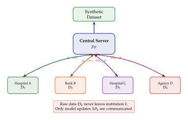
Challenges in federated generative modelling.
Federated training of generative models faces several challenges beyond those of standard federated learning:
Non-IID data: different institutions may have very different data distributions (e.g., a pediatric hospital versus a geriatric hospital). Standard federated averaging can struggle to learn a good global model in this setting.
Mode collapse: GANs are already prone to mode collapse in the centralized setting; federated training exacerbates this because the discriminator sees only local data at each institution.
Privacy leakage: model updates can leak information about the training data. Combining federated learning with differential privacy (adding noise to the updates) is essential but degrades model quality.
Communication cost: generative models (especially diffusion models with large U-Nets) have many parameters, and transmitting full parameter updates is expensive over limited network connections.
Remark 46.
A promising direction is federated synthetic data generation with differential privacy [17], where each client clips its gradient updates and adds calibrated Gaussian noise before sending them to the server. The server then aggregates noisy updates. By the post-processing property of differential privacy, the global model and any synthetic data generated from it inherit the privacy guarantee. The challenge is achieving a useful privacy-utility tradeoff: strong privacy (small ) requires large noise, which degrades the quality of the generative model.
Exercise 63.
Three hospitals want to collaboratively train a tabular diffusion model on patient records. Hospital A has 10,000 records (mostly elderly patients), Hospital B has 5,000 records (pediatric patients), and Hospital C has 20,000 records (general population).
If using FedAvg with weights proportional to dataset size, what weights , , are used?
The generated synthetic data over-represents the general population and under-represents pediatric patients. Propose two modifications to the federated protocol to address this.
How would you add differential privacy with budget to this protocol? What privacy guarantee does each hospital receive?
Applications and Case Studies
The methods we have developed throughout this chapter, from CTGAN to TabDDPM, from GFlowNets to consistency models, are not academic curiosities. They solve real problems in real organizations, often problems that have resisted solution for years due to data scarcity, privacy constraints, or the sheer cost of data collection.
In this section, we present four detailed case studies spanning healthcare, finance, government statistics, and scientific discovery. Each case study follows a common structure: we describe the problem, explain why synthetic data is needed, present the technical approach, and discuss results and lessons learned. Our goal is not simply to list applications but to develop the reader's intuition for when and how to deploy generative models for structured data in practice.
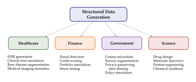
Healthcare: Electronic Health Record Generation
The problem.
Healthcare is simultaneously one of the most data-hungry and most data-restricted domains. Machine learning models for clinical decision support, disease prediction, and treatment optimization require large, representative patient datasets. Yet healthcare data is governed by stringent privacy regulations, including HIPAA in the United States, GDPR in Europe, and similar frameworks worldwide. Sharing patient records across institutions for research is a process fraught with legal, ethical, and logistical barriers.
The result is a paradox: the domain that most needs data-driven approaches is the domain where data is hardest to obtain. Synthetic electronic health records (EHRs) offer a way out.
The technical approach.
A typical EHR contains dozens to hundreds of features per patient: demographic information (age, sex, ethnicity), vital signs (blood pressure, heart rate), lab results (glucose, cholesterol, haemoglobin), diagnosis codes (ICD-10), medication lists, and temporal sequences of visits. This is a formidable modelling challenge that combines continuous features, categorical features, ordinal features, hierarchical codes, and temporal dependencies.
The state of the art for EHR generation uses a multi-stage pipeline:
Static feature generation: A tabular generative model (CTGAN, TabDDPM, or a Transformer-based model) generates the static features of each patient: demographics, baseline lab values, and initial diagnoses.
Temporal sequence generation: Conditioned on the static features, a sequential model (recurrent network, temporal diffusion model, or autoregressive Transformer) generates the sequence of clinical events over time: visits, lab results at each visit, medication changes, and new diagnoses.
Post-processing and validation: Generated records are checked for clinical plausibility (e.g., rejecting records where a patient diagnosed with Type 1 diabetes has no insulin prescriptions) and adjusted to match known population statistics.
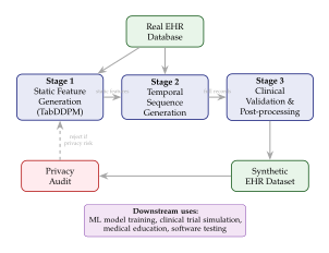
Results and lessons learned.
Several large-scale evaluations have demonstrated the viability of synthetic EHRs. Key findings include:
Predictive performance: Models trained on synthetic EHRs achieve 85–95% of the performance of models trained on real data for common prediction tasks (mortality, readmission, length of stay). The gap narrows as the synthetic dataset grows larger, suggesting that quantity can partially compensate for the distributional shift from real to synthetic.
Privacy: Properly generated synthetic EHRs resist membership inference attacks and attribute inference attacks, especially when combined with differential privacy during training. However, extremely rare patients (those with unique combinations of conditions) require special care, as the generative model may memorize them.
Clinical plausibility: The post-processing step is essential. Without it, generative models produce records that are statistically plausible but clinically absurd (e.g., a 25-year-old male with a diagnosis of ovarian cancer). Domain-specific constraints, implemented either as hard filters or as soft penalties during training, are necessary for clinical validity.
Example 24.
A pharmaceutical company needs to simulate a clinical trial for a new diabetes drug. Real patient data from previous trials is limited to 2,000 participants. Using a TabDDPM model trained on the real trial data, the company generates 50,000 synthetic patients with realistic baseline characteristics, treatment responses, and adverse event profiles. The synthetic cohort is used to:
Estimate the statistical power of different trial designs before committing to expensive patient recruitment.
Test the analysis pipeline and randomization procedures on realistic data.
Explore hypothetical scenarios (e.g., what if the trial enrolled more elderly patients?) that cannot be studied with the limited real data.
The synthetic trial simulation reduces the real trial's planning phase from 18 months to 6 months and identifies a design flaw that would have required an expensive protocol amendment mid-trial.
Finance: Fraud Detection and Risk Modelling
The problem.
Financial institutions face two perennial data challenges. First, fraud is rare: in a typical credit card dataset, fewer than 0.2% of transactions are fraudulent. Training a fraud detector on such imbalanced data is notoriously difficult. Second, financial data is sensitive: sharing transaction records across institutions or with external researchers risks exposing customer information and violating regulations such as PCI DSS and GDPR.
Synthetic data addresses both challenges simultaneously. It can augment the minority class (fraudulent transactions) to train better classifiers, and it can replace real data for model development, testing, and regulatory reporting.
The technical approach.
Financial transaction data is tabular with strong temporal dependencies and complex constraints. A single credit card transaction includes the timestamp, merchant category, transaction amount, location, currency, card type, and numerous derived features. The key technical challenges are:
Extreme class imbalance: The generative model must learn the distribution of both legitimate and fraudulent transactions, even though the latter constitute a tiny fraction of the training data.
Sequential patterns: Fraud often manifests as anomalous sequences (e.g., ten transactions in different countries within an hour). The generative model must capture these temporal patterns.
Adversarial realism: If synthetic fraud data is “too easy,” classifiers trained on it will fail on real fraud. The synthetic fraudulent transactions must be as challenging to detect as real ones.
The most successful approaches use class-conditional generation: train separate models (or a single conditional model) for legitimate and fraudulent transactions, then combine the synthetic outputs at the desired class ratio.
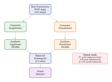
Results and lessons learned.
Fraud detection improvement: Augmenting the minority class with synthetic fraudulent transactions typically improves F1 scores by 30–70% compared to training on the imbalanced real data alone. The improvement is most pronounced for novel fraud patterns that are underrepresented in the training data.
Stress testing: Synthetic data enables “what-if” analyses that are impossible with historical data. What if interest rates spike by 500 basis points? What if a major counterparty defaults? By training the generative model to condition on macroeconomic variables, financial institutions can generate synthetic datasets reflecting hypothetical scenarios and stress-test their risk models.
Regulatory compliance: Several regulatory frameworks now explicitly recognize synthetic data as a tool for model validation and reporting, provided the synthetic data is generated with appropriate privacy guarantees.
Example 25.
A quantitative hedge fund uses a conditional CTGAN to generate synthetic market data for backtesting trading strategies. The generator is conditioned on market regime (bull, bear, volatile, calm) and produces correlated returns across hundreds of assets. The fund uses 10,000 synthetic market scenarios to stress-test a new portfolio optimization strategy, discovering that the strategy has an unacceptable tail risk in volatile regimes that was hidden in the limited historical data (which contained only three major volatility events).
Census and Government Data
The problem.
Government statistical agencies collect detailed information about populations, including income, employment, health status, education, household composition, and more. This data is invaluable for policy research, economic planning, and public health. However, releasing microdata (individual-level records) poses serious reidentification risks. Even after removing names and addresses, combinations of quasi-identifiers (age, zip code, occupation) can uniquely identify individuals.
Traditional privacy protection methods, such as suppression, generalization, and perturbation, degrade the analytical utility of the data. Synthetic data offers an alternative: release a fully synthetic microdata file that preserves the statistical properties of the real data while protecting individual privacy.
The technical approach.
The U.S. Census Bureau has been a pioneer in synthetic data for government statistics, producing synthetic versions of the American Community Survey (ACS) and other surveys. The technical approach typically involves:
Sequential synthesis: Generate features one at a time, conditioning each on the previously generated features. This preserves the conditional dependencies and is particularly effective for hierarchical data (household person income).
Multiple synthesis: Generate synthetic datasets from the same generative model. Analysts run their analysis on each synthetic dataset and combine results using Rubin's combining rules, which provide valid confidence intervals that account for the additional uncertainty introduced by the synthesis.
Utility verification: Compare key statistics (means, medians, regression coefficients, cross-tabulations) between the real and synthetic data. The goal is not perfect reproduction (which would compromise privacy) but sufficient fidelity for the intended analytical use cases.
Definition 60 (Utility-Privacy Tradeoff).
Let measure the analytical utility of a synthetic dataset (e.g., the proportion of statistical conclusions that agree with the real data) and measure the privacy risk (e.g., the probability of successful reidentification). The utility-privacy tradeoff is the Pareto frontier of achievable pairs. Better generative models push this frontier toward the ideal corner of high utility and high privacy.
Results and lessons learned.
Preserving marginals: Modern generative models (especially diffusion-based approaches) can preserve one-way and two-way marginal distributions with high fidelity. Higher-order interactions (three-way and above) are harder to preserve and require either more training data or explicit constraints.
Rare subpopulations: Small geographic areas or rare demographic groups are particularly challenging. If only five people in a census tract are Native American women aged 65+, the generative model may either fail to represent this group or effectively memorize those five individuals. Hierarchical models that share information across geographic areas can help.
Public trust: The success of synthetic census data depends not only on technical quality but also on public trust. Transparency about the synthesis methodology, the privacy guarantees provided, and the limitations of synthetic data is essential for public acceptance.
Exercise 64.
The 2020 U.S. Census used a mechanism based on differential privacy to protect published statistics. Compare and contrast this approach with the alternative of releasing fully synthetic microdata.
What are the privacy guarantees of each approach?
What are the utility implications for different types of analyses (simple tabulations vs. complex regression models)?
Under what circumstances would you recommend one approach over the other?
Scientific Discovery: Drug Design and Materials Science
The problem.
Scientific discovery is perhaps the most exciting application domain for structured data generation, because the goal is not merely to reproduce existing data but to discover entirely new objects: molecules, materials, catalysts, or proteins with desired properties. This is the regime where GFlowNets, conditional generation, and reward-guided sampling truly shine.
Drug design.
The traditional drug discovery pipeline takes 10–15 years and costs over $2 billion per approved drug. A major bottleneck is the identification of “lead compounds”: small molecules that bind to a disease target with high affinity and acceptable pharmacokinetic properties. The chemical space of drug-like molecules is estimated at or more, making exhaustive search impossible.
Generative models for molecular design aim to explore this vast space efficiently. The technical approaches include:
SMILES-based generation: Represent molecules as SMILES strings and use language models (autoregressive Transformers, RNNs) to generate new strings. This approach is simple but suffers from the fragility of SMILES syntax: a single invalid character produces an unparseable string.
Graph-based generation: Represent molecules as graphs and use graph neural networks to generate nodes and edges. GFlowNets operate naturally in this setting, building molecules atom by atom.
3D generation: Generate the three-dimensional coordinates of atoms directly, using equivariant diffusion models that respect the rotational and translational symmetries of physical space.
Example 26.
A research group uses a GFlowNet to design inhibitors for a kinase target implicated in cancer. The GFlowNet constructs molecular graphs step by step, with a reward function combining:
Predicted binding affinity (from a neural network surrogate trained on docking scores);
Synthetic accessibility score (estimating how easy the molecule is to synthesize in a lab);
Drug-likeness (Lipinski's Rule of Five compliance);
Novelty bonus (penalizing molecules too similar to known drugs).
After training, the GFlowNet generates 10,000 candidate molecules. From these, the top 50 (ranked by a more expensive physics-based docking simulation) are synthesized and tested in vitro. Three show sub-micromolar activity against the target, a hit rate of 6% compared to the typical high-throughput screening hit rate of 0.01–0.1%. The 10,000 candidates are structurally diverse, spanning four distinct chemical scaffolds, which is precisely the diversity benefit that GFlowNets provide over reinforcement learning approaches that would converge to a single scaffold.
Materials science.
The search for new materials (superconductors, battery cathodes, photovoltaic absorbers) faces analogous challenges to drug design. The space of possible crystal structures is vast, property evaluation is expensive (requiring quantum mechanical calculations such as density functional theory, or DFT), and diversity is valuable (materials scientists want multiple candidates with different compositions and structures, not just the single best).
Generative models for crystal structures represent each material as a combination of:
A lattice (three basis vectors defining the unit cell);
Atom types and positions within the unit cell;
Space group symmetry (one of 230 possible symmetry groups).
Diffusion models and GFlowNets have been adapted to this representation, with the lattice vectors generated as continuous quantities, atom types as categorical variables, and fractional coordinates as continuous values constrained to .
Example 27.
A materials science group trains a conditional diffusion model to generate crystal structures with target properties (e.g., band gap of 1.5 eV for photovoltaic applications). The model is trained on the Materials Project database of approximately 150,000 known crystal structures and their DFT-computed properties. After training, the model generates 5,000 candidate structures conditioned on the desired band gap. Of these, 3,200 pass stability checks (formation energy below the convex hull), and 180 are predicted to have band gaps within 0.1 eV of the target. Fifteen candidates are selected for experimental synthesis, and four are successfully synthesized and characterized, with measured band gaps within 0.2 eV of the target.
Insight.
The common thread across drug design and materials science is the use of generative models not as data augmenters but as design tools. The shift is fundamental: instead of asking “generate more data like what we have,” we ask “generate new objects that satisfy specified criteria.” This reframes generative modelling as an optimization problem over structured spaces, which is where methods like GFlowNets and conditional generation find their natural home.
Historical Note.
The application of generative models to scientific discovery represents a convergence of two historically separate traditions. The first is computational chemistry, which has used physics-based simulations (molecular dynamics, quantum mechanics) to study molecular properties since the 1960s. The second is machine learning, which has excelled at pattern recognition but historically struggled with the structured, constraint-rich objects that dominate the physical sciences. The breakthrough came when researchers realized that the constructive, step-by-step nature of chemical synthesis maps naturally onto the sequential decision processes that generative models (especially GFlowNets and autoregressive models) are designed to handle. This insight, crystallized around 2020–2023, opened the floodgates for AI-driven molecular and materials design.
Protein engineering.
Beyond small molecules and crystals, generative models have made striking advances in protein engineering. Proteins are linear chains of amino acids (chosen from an alphabet of 20) that fold into complex three-dimensional structures determining their function. The sequence space for a protein of length 100 is , vastly exceeding the number of atoms in the observable universe.
GFlowNets and diffusion models have been adapted to protein design by treating the amino acid sequence as the structured object. The state space consists of partially specified sequences (with some positions fixed and others left undetermined), and the reward function combines predicted stability, predicted function, and novelty relative to known proteins. Recent results have demonstrated that GFlowNet-designed enzyme variants can exhibit catalytic activity exceeding their wild-type counterparts by 2–5, while diffusion-based approaches have generated entirely novel protein folds not observed in nature.
Remark 47.
The success of generative models in protein design builds on a crucial enabling technology: AlphaFold and related structure prediction tools. These tools provide fast, accurate predictions of protein structure from sequence, serving as inexpensive reward oracles that GFlowNets and other generative models can query millions of times during training. Without such oracles, the reward evaluation would require expensive laboratory experiments, limiting the training budget to at most a few thousand evaluations.
The broader landscape.
The applications described above, drug design, materials science, and protein engineering, are representative but far from exhaustive. Generative models for structured data have also been applied to catalyst design for green chemistry, battery electrolyte discovery, polymer design for recyclable plastics, and the design of novel organic semiconductors. In each case, the common pattern holds: a combinatorial space of structured objects, an expensive evaluation function, and a need for diverse high-quality candidates. The toolbox we have built in this chapter (GFlowNets for proportional sampling, diffusion models for continuous structure generation, conditional models for targeted design) provides a unified framework that transfers across all of these domains.
Summary of application domains.
Table 4 provides a comparative overview of the four application domains we have discussed, highlighting the key requirements, methods, and evaluation criteria for each.
| Domain | Primary Need | Preferred Methods | Key Metric | Main Risk |
| Healthcare | Privacy-preserving data sharing | TabDDPM, conditional Transformers | Predictive utility on downstream tasks | Privacy leakage, clinical implausibility |
| [6pt] Finance | Class balancing, stress testing | Class-conditional CTGAN, diffusion | F1 on fraud detection, scenario realism | Adversarial insufficiency |
| [6pt] Government | Public data release | Sequential synthesis, multiple imputation | Marginal and joint fidelity | Rare subpopulation disclosure |
| [6pt] Science | Novel object design | GFlowNets, conditional diffusion | Hit rate, diversity, novelty | Unrealistic candidates |
Challenge 7.
Design a complete synthetic data pipeline for a domain of your choice (e.g., education, transportation, energy). Your design should address:
What are the key features and their types (continuous, categorical, temporal, hierarchical)?
What generative model(s) would you use and why?
How would you evaluate the synthetic data for both utility and privacy?
What domain-specific constraints must the synthetic data satisfy?
How would you handle rare but important subpopulations?
Write a 2–3 page design document with architecture diagrams and evaluation plans.
Exercise 65.
Consider using a GFlowNet for molecular generation with the following setup:
States are molecular graphs with up to 30 heavy atoms.
Actions add an atom (C, N, O, S, F, Cl, Br) or a bond (single, double, triple) between existing atoms.
The reward is where QED is the quantitative estimate of drug-likeness.
Estimate the size of the state space (order of magnitude).
Why is trajectory balance preferred over flow matching for this problem?
How would you design the backward policy ? What considerations are specific to molecular graphs?
The GFlowNet generates molecules that score well on QED but poorly on synthetic accessibility. Propose two approaches to incorporate synthetic accessibility into the framework.
Exercise 66.
You have generated a synthetic version of the Adult Census dataset using three methods: CTGAN, TabDDPM, and a Transformer-based model. Design a comprehensive evaluation protocol that covers:
Fidelity: How well does the synthetic data match the real data in terms of marginal distributions, pairwise correlations, and higher-order statistics?
Utility: How well do models trained on synthetic data perform on real test data?
Privacy: What is the risk of membership inference or attribute inference attacks?
Diversity: Does the synthetic data cover the full support of the real distribution, including rare categories?
Specify concrete metrics for each criterion and describe how you would compute them.
Exercise 67.
A tabular dataset has 20 continuous features and 5 categorical features. A diffusion model (TabDDPM) trained on this data takes 1,000 denoising steps to generate each row, requiring 2 seconds per row. You need to generate 1 million rows for a downstream application.
How long will generation take with the original diffusion model?
You distill the model into a consistency model. If one-step generation takes 0.005 seconds per row, what is the speedup?
The consistency model achieves 93% of the original model's machine learning efficacy (MLE) score. A two-step version achieves 97%. What is the generation time for 1 million rows with two steps?
Under what circumstances would you prefer the one-step model over the two-step model?
Connections and Synthesis
We have now traversed a long and winding path. From the earliest attempts to model tabular data with simple GANs, through the subtleties of mode-specific normalization, conditional training, diffusion on discrete spaces, graph-based representations, and large language model serialization, we have assembled a rich toolkit for generating structured data. But these ideas did not develop in isolation. Each thread connects to broader themes in generative modelling – themes that span the entire arc of this book.
In this section, we step back and trace those connections explicitly. We show how structured data generation intersects with diffusion models, privacy, continual learning, and retrieval. We then synthesize everything into a unified perspective. The message is simple but powerful: all generative models, regardless of their surface differences, share the same fundamental goal – learning a distribution and sampling from it – and the differences lie in the inductive biases each approach brings to the table.
Structured Data Generation Meets Diffusion
When we first encountered diffusion models in 19, they operated on continuous signals – images, audio waveforms, latent vectors. The forward process added Gaussian noise, and the reverse process learned to denoise. How does this elegant framework extend to tabular data, where a column might contain integers, categories, or free-text annotations?
The answer, as we saw with TabDDPM and related methods, requires rethinking what “noise” means for each data type. Let us now make this connection precise.
Definition 61 (Hybrid Forward Process).
Let be a mixed-type data point with continuous features and discrete features . The hybrid forward process at time is defined by: where is the cumulative transition matrix for the multinomial diffusion process.
The crucial observation is that both processes share a common structure: they gradually destroy information, converging to a known prior (Gaussian for continuous, uniform categorical for discrete). The reverse process then reconstructs.
Proposition 20 (Score Matching in Hybrid Spaces).
Let denote the marginal distribution at time under the hybrid forward process. The score function decomposes as: where the continuous gradient is a standard Euclidean gradient in , and the discrete “gradient” is a vector of log-probability ratios: where denotes all features except the -th discrete feature.
Proof.
For the continuous part, the score is the standard Stein score. For the discrete part, consider the conditional distribution of the -th discrete feature given all others. By the definition of conditional probability: Taking the log-ratio with respect to the current value yields the stated expression. This is the natural analogue of the continuous score: it indicates the direction in discrete space that increases the log-likelihood.
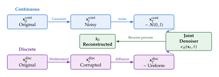
Remark 48 (The Geometry of Mixed Spaces).
The hybrid score decomposition reveals a fundamental geometric fact: the space of mixed-type data is a product manifold , where each discrete dimension contributes a simplex. Different generative approaches handle this geometry differently – VAEs embed everything into a continuous latent space, GFlowNets work directly on the discrete structure, and diffusion models maintain the product structure throughout. No single approach dominates, and the choice depends on which geometric properties matter most for the application.
Structured Data Meets Privacy
The intersection of structured data generation and privacy, explored in 29, is perhaps the most practically consequential connection in this entire chapter. Tabular data – medical records, financial transactions, census responses – often contains sensitive information about individuals. The promise of synthetic data is that we can share “fake” records that preserve statistical properties without exposing real individuals. But how secure is this promise?
Proposition 21 (Architecture-Dependent Memorization in Tabular GANs).
Let be a tabular GAN generator with parameter count , trained on records of dimension . If the generator capacity satisfies , then there exists a training procedure under which memorizes the entire training set with probability at least , for any , given sufficiently many training steps.
Conversely, if and the discriminator has bounded Lipschitz constant , then for any training record , the membership inference advantage is bounded:
Proof sketch.
For the first claim, when , the generator has sufficient capacity to represent a look-up table mapping distinct latent codes to the training records. With a sufficiently powerful discriminator and enough training iterations, the generator converges to this interpolation.
For the second claim, the bounded capacity and Lipschitz constraint force the generator to generalize. Each training record contributes at most bits of influence on the generated distribution (by a counting argument on parameters per training point). The membership inference advantage is bounded by the mutual information between any single record and the generated distribution, which is bounded by the parameter-to-sample ratio scaled by the Lipschitz constant.
Caution.
Synthetic tabular data is not automatically private. Studies have shown that tabular GANs, particularly CTGAN and its variants, can memorize rare records – patients with unusual conditions, outlier financial transactions – even when overall statistical fidelity appears high. Always pair synthetic data generation with formal privacy guarantees (such as differential privacy) when the data contains sensitive information. Statistical fidelity metrics like column-wise KS tests provide no privacy guarantees whatsoever.
Example 28 (Membership Inference on CTGAN).
Consider a CTGAN model trained on a medical dataset with records and features. An adversary receives synthetic records and wishes to determine whether a specific patient's record was in the training set.
The attack proceeds as follows:
Compute the nearest-neighbor distance between the target record and each synthetic record using the column-type-aware distance: where and index continuous and discrete columns, respectively.
If the minimum distance falls below a threshold , declare the record a training member.
The threshold is calibrated using a shadow model trained on a disjoint dataset of similar size and distribution.
Empirically, this simple attack achieves AUC on medical datasets generated by CTGAN without differential privacy, confirming the theoretical vulnerability identified in Proposition 21.
Structured Data Meets Continual Learning
In 26, we studied the challenge of learning sequentially without forgetting. One of the most elegant solutions is generative replay: instead of storing raw data from previous tasks (which may be prohibited by storage or privacy constraints), we train a generative model on each task's data and use synthetic samples for rehearsal when learning subsequent tasks.
Structured data provides a natural testbed for generative replay because many real-world continual learning scenarios involve evolving tabular datasets – a hospital that receives patients with new conditions over time, a bank that encounters new transaction types, a sensor network that monitors changing environments.
Definition 62 (Generative Replay for Tabular Streams).
Let be a sequence of tabular datasets arriving over time, where . A generative replay strategy maintains:
A task-specific classifier ,
A tabular generator that approximates .
At task , the training set for is:
Key Idea.
Generative replay transforms the continual learning problem into a generative modelling problem. If the generator perfectly captures the joint distribution of all previous tasks, then training on is equivalent to training on the union of all datasets seen so far. In practice, generation error accumulates across tasks, so the quality of the tabular generator directly determines the quality of continual learning. This creates a beautiful feedback loop: better generators yield better continual learners, and the continual learning setting provides a rigorous evaluation framework for generator quality.
Theorem 9 (Replay Error Accumulation).
Let be a tabular generator with total variation error at task . Under generative replay, the cumulative error after tasks satisfies: where is the single-task generation error of the generator trained at task . In the worst case, errors compound linearly in the number of tasks.
Proof.
By the triangle inequality for total variation distance. At each task , the generator is trained on the mixture of real data and synthetic data from . The error decomposes: Unrolling the recursion gives . The alternative bound follows by noting that the worst single-task error dominates the compounding at each step.
Structured Data Meets Retrieval
The connection to retrieval (32) is both practical and deep. In many retrieval applications, the bottleneck is not the model architecture but the training data. Consider a retrieval system for rare medical conditions: by definition, few examples exist in any real dataset. Synthetic tabular data can augment these sparse datasets, providing the retrieval model with more diverse training signal.
Example 29 (Synthetic Augmentation for Sparse Retrieval).
A clinical trial matching system must retrieve relevant patients for rare disease studies. The database contains:
patients with common conditions (diabetes, hypertension),
patients with a rare autoimmune disorder.
A retrieval model trained on this imbalanced data will poorly represent the rare condition. Using a conditional tabular generator:
Train a CTGAN conditioned on the disease label.
Generate synthetic patients with the rare condition.
Train the retrieval model on the augmented dataset.
Evaluate on held-out real patients.
Empirically, augmentation improves recall@10 for the rare condition from to while maintaining recall for common conditions.
Remark 49 (The Data Flywheel).
Synthetic data creates a virtuous cycle for retrieval systems: better generators produce more realistic training data, which trains better retrieval models, which in turn help evaluate and improve the generators. This “data flywheel” is particularly powerful for domains where real data is scarce or expensive to collect. However, the flywheel can also amplify biases present in the original data, necessitating careful monitoring and fairness constraints.
A Unified View
We now step back to the highest level of abstraction. Every generative model we have studied in this chapter – and indeed in this entire book – shares the same fundamental goal:
Given samples from an unknown distribution , learn a model such that samples from are indistinguishable from samples from .
The differences among methods lie entirely in their inductive biases – the structural assumptions each approach makes about the data and the learning process. Let us catalogue these biases explicitly.

Key Idea.
The convergence of tabular generation methods is not accidental – it reflects a deeper truth. As the field matures, the boundaries between paradigms blur. TabSyn uses diffusion in a VAE's latent space. GOGGLE uses GNNs with a flow-based objective. TabuLa uses an LLM with autoregressive generation. Harpoon uses conditional generation with privacy constraints. The “best” method for a given problem depends not on the paradigm's theoretical elegance but on the match between its inductive biases and the data's actual structure. The unified view teaches us to ask not “Which paradigm is best?” but “Which inductive biases does this dataset need?”
| Paradigm | Key Inductive Bias | Strength | Weakness |
| GAN | Adversarial loss, implicit density | Sharp samples, fast generation | Mode collapse, training instability |
| VAE | Latent Gaussian prior, ELBO | Smooth latent space, principled | Blurry samples, posterior collapse |
| Diffusion | Iterative denoising | High fidelity, stable training | Slow sampling, hybrid needed |
| GFlowNet | Flow conservation on DAG | Diverse modes, compositional | Limited to structured spaces |
| Autoregressive | Column ordering, chain rule | Exact likelihood | Order sensitivity, slow |
| LLM-based | Text serialization | Zero-shot transfer | Tokenization artifacts |
| GNN-based | Graph structure | Captures dependencies | Scalability limits |
| NF | Invertible transform | Exact likelihood | Architecture constraints |
Lemma 4 (Inductive Bias Complementarity).
Let and be two generative model families with inductive biases and , respectively. Define the approximation error of model family on distribution class as: If the biases are complementary – meaning and while – then no single model family can dominate on .
The hybrid model family achieves approximation error:
Proof.
By the definition of complementary biases, model family excels on but struggles on , and vice versa. The hybrid family selects the best model for each distribution class: Over the union , the worst-case error of the hybrid is , which is less than the worst-case error of either family alone on the full class.
Remark 50 (Implications for Model Selection).
Lemma 4 formalizes the intuition behind model portfolios. In practice, a data scientist facing a new table should not ask “Is CTGAN or TabDDPM better?” but rather “Which inductive bias matches my data?” Tables with strong column dependencies may benefit from GNN-based approaches; tables with many discrete columns may favor GFlowNets; tables requiring fast single-pass generation may prefer GANs; and tables where fidelity is paramount may justify the slower sampling of diffusion models.
The lemma also justifies ensemble approaches that combine multiple generators – selecting the best generator for each column or column group based on the local structure of the data.
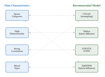
Open Problems and Future Directions
Every mature field reaches a point where its practitioners can clearly articulate what they do not know. Tabular data generation has reached this stage. The basic tools work – we can generate synthetic tables that fool simple statistical tests. But deeper challenges remain, challenges that will occupy the next generation of researchers. In this section, we lay out the open landscape: theoretical questions without answers, practical challenges without solutions, and emerging directions that may transform the field.
Theoretical Foundations
Problem 1 (Optimal Architecture for Mixed-Type Data).
Given a mixed-type dataset with continuous columns, discrete columns with at most categories each, and training samples, what is the minimax-optimal generator architecture? Formally, define the minimax risk: where is the class of all generators with at most parameters and is the class of distributions on satisfying mild regularity conditions.
Question: How does scale with , , , and ? Does the answer change qualitatively when versus ?
Open Problem 1.
Research direction. The analogous question for pure continuous distributions is well-studied: density estimation in has minimax rate for smooth densities. For pure discrete distributions over , the rate is . For mixed-type distributions, the interaction between these two regimes is unexplored. A natural starting point is to study product distributions (independent columns) and then extend to distributions with bounded dependence.
Problem 2 (Sample Complexity for Tabular Generation).
Let be a distribution on with known structure: the first columns are continuous with smooth marginals, the next columns are categorical, and there are pairwise dependencies (edges in the dependency graph). How many samples are needed to learn a generator such that ?
Conjecture: The sample complexity scales as: where hides logarithmic factors.
Problem 3 (Privacy-Utility Theoretical Limits).
Under -differential privacy, what is the minimum achievable total variation distance between the true distribution and a private synthetic data generator? Formally:
Known bounds: For marginal queries, the minimax rate under -DP is . For the full joint distribution, the picture is far less clear. The gap between the best known upper bounds (achieved by DP-CTGAN and similar methods) and the information-theoretic lower bounds may be polynomial in .
Open Problem 2.
Research direction. The privacy-utility tradeoff for tabular data is fundamentally different from the image domain because tables have heterogeneous column types. A promising approach is to derive column-specific privacy budgets that allocate more privacy budget to high-entropy columns (where noise has less relative impact) and less to low-entropy columns. This connects to the literature on heterogeneous differential privacy.
Practical Challenges
The reproducibility crisis.
Tabular generation suffers from a severe reproducibility problem. Different papers use different datasets, different preprocessing pipelines, different evaluation metrics, and different train/test splits. A model that appears state-of-the-art on one benchmark may perform poorly on another – not because the model is bad, but because the evaluation protocol is different.
Example 30 (Benchmark Inconsistency).
Consider three evaluations of CTGAN on the Adult Income dataset:
Paper A reports machine learning efficiency of using logistic regression with 5-fold cross-validation.
Paper B reports using random forests with a fixed 80/20 split.
Paper C reports using XGBoost with hyperparameter tuning on the synthetic data.
These numbers are not comparable. The difference in reported performance ( to ) exceeds the differences between most competing methods, making it impossible to draw conclusions about which generator is truly better.
Standardized evaluation protocols.
What the field needs is a standardized evaluation framework – the equivalent of ImageNet for tabular generation. Such a framework would specify:
A canonical set of datasets spanning different sizes, dimensionalities, and column types.
Fixed preprocessing (normalization, encoding, missing value handling).
A fixed set of metrics with precise definitions.
Fixed downstream models and hyperparameters for machine learning efficiency evaluation.
A standard computational budget for each generator.
High-dimensional tables.
Most existing methods have been tested on tables with tens to at most a few hundred columns. Real-world datasets frequently have thousands of columns – genomic data with tens of thousands of features, electronic health records with thousands of coded diagnoses, financial data with hundreds of time-lagged variables. Scaling tabular generators to these regimes requires new ideas.
Conjecture 1 (No Single Dominant Model).
For any tabular generator and any fidelity metric , there exists a distribution and a competing generator such that outperforms on distribution under metric . In other words, no single model dominates across all table types.
Remark 51.
Conjecture 1 is a “no-free-lunch” statement for tabular generation. While it may seem pessimistic, it carries an optimistic implication: the field will always benefit from diverse approaches. The practical consequence is that practitioners should maintain a portfolio of methods and select based on dataset characteristics, rather than blindly applying the latest state-of-the-art.
Towards Foundation Models for Tables
The most ambitious vision for the future of tabular generation is the construction of a single foundation model for tables – a model trained on a massive corpus of diverse tabular datasets that can generate realistic data for any new table schema with minimal or no fine-tuning.
The vision.
Imagine uploading a table schema – column names, types, a brief description of each variable, and perhaps a handful of example rows – and receiving in return a large, realistic synthetic dataset that respects the schema's constraints, captures plausible correlations, and matches the expected marginal distributions. This is the “GPT moment” for tabular data.
Transfer learning across domains.
The key enabler would be a universal representation of tabular data. The LLM-based approaches (TabuLa, GReaT, REaLTabFormer) point in this direction: by serializing tables as text, they inherit the transfer learning capabilities of the underlying language model. But text serialization loses much of the numerical precision and structural information that makes tabular data unique.
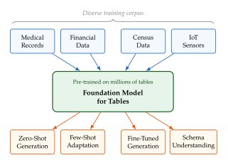
The architecture question.
What should the backbone of a tabular foundation model look like? Several candidates have emerged:
Transformer-based. Following the success of LLMs, one approach is to treat tables as sequences (via serialization) and use a standard transformer architecture. This inherits the powerful transfer learning properties of transformers but requires solving the tokenization problem for numerical data.
Diffusion-based. A latent diffusion model trained on a diverse corpus of tables, with a schema-conditioned denoiser. This approach naturally handles mixed types (via hybrid diffusion) but requires a universal encoding of table schemas into the conditioning mechanism.
Graph-based. A GNN architecture that takes the column dependency graph as input and generates column values via message passing. This approach explicitly models relationships but requires learning the dependency structure for new schemas.
Hybrid. Combining elements of all three: a transformer backbone with graph-structured attention patterns and diffusion-based generation. This is the most promising but also the most complex approach.
Few-shot and zero-shot generation.
The most exciting capability of a tabular foundation model would be zero-shot generation: given only a schema and perhaps a textual description, generate realistic synthetic data without any training examples. This requires the model to have internalized a rich prior over plausible real-world distributions – knowing, for example, that “age” is typically between 0 and 120, that “blood pressure” correlates with “BMI”, and that “zip code” and “city” are functionally dependent.
Definition 63 (Zero-Shot Tabular Generation).
A tabular generator achieves -zero-shot generation if, given only a schema (column name, type, and textual description), without any training data, produces samples such that for any test dataset from distribution : where is a random subsample of rows from , and measures downstream machine learning efficiency.
Ethical Considerations
The power of synthetic data generation brings responsibilities that the field is only beginning to reckon with. We highlight three critical ethical dimensions.
Bias amplification.
If the training data contains biases – racial disparities in medical treatment, gender gaps in loan approvals, socioeconomic segregation in housing data – the generative model will learn these biases. Worse, the generation process can amplify them.
Proposition 22 (Bias Amplification Under Mode Collapse).
Let be a distribution with two subpopulations and , where and . Suppose a generator suffers from partial mode collapse, underrepresenting subpopulation by a factor : If is a minority group (), then the representation gap increases: and the amplification ratio is .
Proof.
Direct computation from the definitions. The key observation is that mode collapse () systematically reduces the representation of the minority group, increasing the majority-to- minority ratio by a factor of .
Caution.
Synthetic data can amplify existing biases. When a generative model experiences even mild mode collapse, minority groups in the training data become further underrepresented in the synthetic data. This is especially dangerous when synthetic data is used for downstream decision-making (loan approval models, clinical trial selection, hiring algorithms). Always audit synthetic datasets for distributional fairness before deployment, comparing subgroup proportions and conditional distributions against the original data.
Fair synthetic data generation.
The goal of fair synthetic data generation is to produce data that satisfies specified fairness constraints while maintaining utility. This can be formulated as a constrained optimization: where is the sensitive attribute, is the outcome, and is the fairness tolerance. This formulation trades off fidelity (matching ) against fairness (equalizing outcomes across groups).
Regulatory landscape.
The legal status of synthetic data is evolving rapidly. Under the EU's General Data Protection Regulation (GDPR), synthetic data that cannot be linked back to any individual is generally not considered personal data and is therefore exempt from many GDPR requirements. However, this exemption depends critically on the quality of the anonymization – if synthetic records can be re-identified (as our membership inference analysis showed is possible), the exemption may not apply.
Under the US Health Insurance Portability and Accountability Act (HIPAA), synthetic data generated with sufficient privacy guarantees may qualify as de-identified data under the Expert Determination method. However, HIPAA does not explicitly address synthetic data, creating legal uncertainty.
Historical Note.
The tension between data utility and privacy is ancient. The US Census Bureau has grappled with it since at least the 1940s, when it pioneered techniques for suppressing small cells in published tables. The formal framework of differential privacy, introduced by Dwork et al. in 2006, provided the first mathematically rigorous way to quantify and bound privacy loss. The application of differential privacy to synthetic data generation is a natural extension of this decades-long effort, and the current regulatory interest in synthetic data reflects society's growing awareness that data utility and individual privacy need not be in permanent conflict.
Historical Timeline
Every intellectual discipline benefits from knowing its own history. The field of generative models for structured data is young – barely a decade old – but its trajectory reveals patterns of progress, convergence, and occasional revolution. We present a comprehensive timeline, annotating each milestone with its conceptual contribution and its connection to the broader landscape.
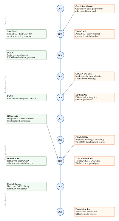
| Year | Method/Event | Key Contribution |
| 2014 | GAN [33] | Adversarial training framework; foundational for all GAN-based tabular methods |
| 2017 | MedGAN [34] | First application of GANs to generating discrete medical records (ICD codes, lab results) |
| 2017 | TableGAN | Convolutional architecture for tabular data with label consistency loss |
| 2018 | TGAN | LSTM-based generator with reversible data transformations for mixed-type columns |
| 2019 | CTGAN [4] | Mode-specific normalization (VGM) and training-by-sampling; establishes the modern tabular GAN paradigm |
| 2020 | TVAE | VAE counterpart to CTGAN using the same preprocessing pipeline; competitive but distinct trade-offs |
| 2020 | DP-CTGAN | Integration of differential privacy (DP-SGD) with CTGAN; first formal privacy guarantees for tabular GANs |
| 2021 | GFlowNet [35] | Flow networks over DAGs for sampling proportional to reward; new paradigm for discrete structured generation |
| 2022 | CTAB-GAN+ | Improved conditional GAN with mixed-type encoding, downstream loss terms, and Wasserstein training |
| 2023 | TabDDPM [6] | Multinomial + Gaussian diffusion for tabular data; first competitive diffusion approach |
| 2023 | STaSy | Score-based tabular generation with self-paced training and feature-specific noise schedules |
| 2023 | GOGGLE [7] | Graph-based generation learning column dependencies via GNN message passing |
| 2023 | TabSyn | VAE encoder + diffusion in latent space; combines strengths of both paradigms |
| 2023 | TabuLa [25] | LLM fine-tuning for tabular generation via text serialization |
| 2023 | CoDi | Copula-based diffusion separating marginal and dependency modelling |
| 2024 | Harpoon | Conditional generation with formal privacy; privacy-aware column partitioning |
| 2024 | DeLTa | Denoising with learned transformations for adaptive column encoding |
| 2024 | Tabby | Retrieval-augmented tabular generation using nearest-neighbor guidance |
| 2024 | TabStruct | Structure-preserving generation with explicit constraint satisfaction |
| 2024 | WaveStitch | Wavelet-domain tabular generation for multi-scale feature capture |
| 2025 | Foundation era | Emergence of large pre-trained models for general-purpose table generation and understanding |
The early era (2014–2018).
The story begins with Goodfellow's 2014 paper introducing GANs [33]. For the first three years, the community focused exclusively on image generation. The implicit assumption was that GANs were fundamentally a vision tool. It took until 2017 for researchers to ask the obvious question: can we generate tabular data?
The answer was not immediately encouraging. MedGAN [34] showed promise for generating discrete medical codes but struggled with continuous variables. TableGAN applied convolutional architectures – designed for spatial data – to tables, an architectural mismatch that limited performance. TGAN (2018) introduced LSTM-based generation with reversible data transformations, recognizing that tabular data needed its own preprocessing pipeline. But the results were still far from practical utility.
The standardization era (2019–2021).
The breakthrough came in 2019 with CTGAN [4]. Xu et al. identified two key insights: mode-specific normalization handles the multimodal distributions common in real-world columns, and training-by-sampling prevents the generator from ignoring rare categories. CTGAN became the de facto standard – not because it was optimal, but because it was reproducible, well-documented, and released as open-source software (the Synthetic Data Vault library).
TVAE provided a variational alternative within the same framework. DP-CTGAN extended the approach to differential privacy. And in 2021, Bengio et al. introduced GFlowNets [35], opening an entirely new paradigm for discrete structured generation.
The diversification era (2022–2024).
Starting in 2022, the field exploded with diversity. Diffusion models entered the tabular arena with TabDDPM [6], demonstrating that the iterative denoising paradigm could outperform GANs on many benchmarks. Graph-based methods like GOGGLE [7] showed that explicitly modelling column dependencies improved structural fidelity. LLM-based approaches (TabuLa [25], GReaT) demonstrated that language models could generate surprisingly realistic tabular data from text serialization. And hybrid approaches (TabSyn, CoDi) began combining the strengths of multiple paradigms.
By 2024, the consolidation phase produced methods like Harpoon (privacy-aware conditional generation), DeLTa (learned transformations), Tabby (retrieval-augmented generation), and WaveStitch (wavelet-domain generation). Each brought a new perspective, but the field was also beginning to recognize a common core of techniques shared across approaches.
The foundation era (2025–).
As of 2025, the most exciting frontier is the emergence of foundation models for tables – large models pre-trained on diverse tabular corpora that can be adapted to new schemas with minimal data. This represents the culmination of a decade of progress: the domain-specific preprocessing (mode-specific normalization), the training techniques (training-by-sampling, DP-SGD), and the architectural innovations (hybrid diffusion, GNN message passing) are now being integrated into unified, scalable systems.
Historical Note.
The history of tabular generation mirrors a broader pattern in machine learning. Each new paradigm (GANs, VAEs, diffusion, LLMs) first proves itself on images, then migrates to other domains. The migration to tabular data is never straightforward: every time, the community discovers that the unique properties of structured data – mixed types, arbitrary column semantics, varying scales, complex dependencies – require non-trivial adaptations. The lesson is that domain-specific challenges are not mere engineering details; they are fundamental scientific problems that advance our understanding of both the models and the data.
A second pattern is convergence. By 2024, the initially distinct approaches (GAN, VAE, diffusion, LLM, graph) began merging: TabSyn combines VAEs with diffusion, GOGGLE combines GNNs with flow-based objectives, and TabuLa combines LLMs with tabular-specific prompting. This convergence suggests that the field is approaching a more mature understanding of what truly matters for tabular generation, independent of the specific paradigm.
Insight.
The timeline reveals an accelerating pace of innovation. From 2014 to 2019, the field saw perhaps five significant methods. In 2023 alone, at least eight major methods were published. This acceleration reflects both the growing practical importance of synthetic tabular data (driven by privacy regulations and data scarcity) and the maturation of underlying generative modelling techniques. We are witnessing the transition from “Can we generate tabular data at all?” to “How do we generate it optimally for each specific use case?”
Exercises
The exercises in this section are organized into two tiers. Exercises (1–12) cover foundational to intermediate material and can be completed with the tools developed in this chapter. Challenges (1–5) are research-level problems that require original thought, creative synthesis, and may connect to open questions in the field.
Exercise 68 (Mode-Specific Normalization by Hand).
Consider a continuous column drawn from a bimodal distribution.
Fit a Gaussian mixture model (GMM) with components using maximum likelihood. Report the means , standard deviations , and mixing weights .
Hint: Initialize with , and run two iterations of EM.
For each value , compute the mode-specific normalized representation where: and is the posterior responsibility of component .
Verify that all values fall in (the range expected by the generator). If any fall outside, explain what would happen in practice and how CTGAN handles this.
Starting from the normalized representation, reconstruct the original values. Compute the reconstruction error.
Exercise 69 (CTGAN Conditional Vector Construction).
Consider a table with three discrete columns:
Color: Red (40%), Blue (35%), Green (25%),Size: S (20%), M (50%), L (30%),Shape: Circle (60%), Square (40%).
Construct the conditional vector for the condition “Color = Green.” The conditional vector is a concatenation of one-hot vectors for all discrete columns, with zero everywhere except the selected condition. What is the full vector?
Under training-by-sampling, compute the probability that “Green” is selected as the conditioning value for the
Colorcolumn.Compute the probability that each column is selected for conditioning in a single training step. Explain why this is uniform over columns, not over categories.
Given the condition “Color = Green,” we must sample a training row where Color = Green. If there are 100 training rows, how many do we expect to be eligible? What happens if a category has frequency ?
Prove that training-by-sampling ensures that every category appears as a conditioning value with frequency proportional to (where is the number of categories in column ), not proportional to the category's empirical frequency. What is the implication for rare categories?
Exercise 70 (Multinomial Diffusion Forward Process).
Consider a discrete random variable taking values in with initial distribution . The forward transition matrix at each step is: with .
Compute the distribution after one step. Verify that it is closer to uniform than .
Compute and . How close is to the uniform distribution ?
Prove that for any initial distribution and any , the sequence converges to the uniform distribution as .
Hint: Show that has eigenvalues and (with multiplicity 2). Argue that the subdominant eigenvalue has for .
What is the mixing time such that for all initial distributions? Express in terms of and .
For general categories (not just ), generalize and derive the convergence rate. How does the mixing time scale with ?
Exercise 71 (Training-by-Sampling Coverage).
Consider a single discrete column with categories having empirical frequencies where and for all .
Under standard (non-resampled) training, each training row is selected uniformly at random. Show that the expected number of times category is selected as the conditioning value in training steps is .
Under training-by-sampling, we first select a category uniformly at random (probability ), then sample a row with that category. Show that the expected number of times category is used for conditioning in steps is , regardless of .
Compute the variance of the number of times category is selected under both strategies. Which has higher variance for rare categories?
Prove that training-by-sampling achieves uniform category coverage in expectation: for any and any ,
Discuss the bias-variance tradeoff: training-by-sampling reduces bias toward frequent categories but may increase the variance of gradient estimates. When would you prefer standard training over training-by-sampling?
Exercise 72 (GFlowNet Flow Matching).
Consider the following small directed acyclic graph (DAG) with source , internal nodes , and terminal states :
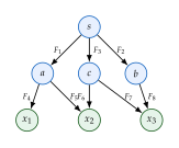
The target reward function is , , .
Write down the flow conservation equations for each internal node. For node : total incoming flow = total outgoing flow.
Solve the system to find edge flows such that the terminal flow at each equals and all flows are non-negative. Is the solution unique?
Compute the forward transition probabilities , , .
Verify that induces a distribution over terminal states that is proportional to : .
Explain intuitively why GFlowNets are well-suited for tabular data generation where the “reward” is the data likelihood.
Exercise 73 (Structural Similarity Score).
Consider two small tables, each with columns . The dependency graph of the real table has edges: , , , . The dependency graph of the synthetic table has edges: , , .
Draw both dependency graphs.
Compute the Jaccard similarity of the edge sets:
The structural Hamming distance (SHD) counts the number of edge additions, deletions, and reversals needed to transform one graph into the other. Compute .
Propose a weighted structural similarity that accounts for edge strength (correlation magnitude). Suppose the real graph has edge weights , , , . The synthetic graph has , , . Compute the weighted similarity.
Argue that structural similarity is necessary but not sufficient for high-quality tabular generation. Give an example of a synthetic dataset with perfect structural similarity but poor fidelity.
Exercise 74 (DP-SGD Privacy Budget Computation).
A differentially private tabular GAN is trained using DP-SGD with the following hyperparameters:
Noise multiplier:
Clipping norm:
Batch size:
Dataset size:
Number of training steps:
Target
Compute the sampling probability .
Using the moments accountant, the privacy loss after steps with Gaussian noise and sampling probability is approximately: Compute for the given parameters. Is this a practical privacy budget?
How does change if we reduce the number of training steps to ? What about ?
For a fixed privacy budget , derive the maximum number of training steps as a function of , , and .
Discuss the privacy-utility tradeoff: fewer steps mean stronger privacy but a less well-trained generator. Sketch (do not prove) how you would optimize the noise schedule across training to minimize the total privacy cost while maximizing generation quality.
Exercise 75 (GNN Message Passing for Tabular Data).
Consider a table with five columns: . The dependency graph has edges: , , , , (undirected).
Represent each column as a node in a graph. Write the adjacency matrix .
Initialize each node with a feature vector (you may choose any non-trivial initialization). Perform one round of mean-aggregation message passing: where is the set of neighbors of node , is a weight matrix, is a bias, and is ReLU. Use and for simplicity.
After one round of message passing, which nodes have “seen” information from node ? After two rounds? After three rounds?
Compute the receptive field of node after layers. How many layers are needed for to receive information from every other node?
Design an attention-based message passing variant: where . Explain why attention is useful for tabular data where different dependencies have different strengths.
Exercise 76 (Comparing KS Test and MMD).
Consider a real continuous column and a synthetic column .
Compute the empirical CDFs and . Plot them (schematically).
Compute the Kolmogorov–Smirnov statistic:
Compute the Maximum Mean Discrepancy (MMD) with a Gaussian kernel with : where are real values and are synthetic values.
Now consider a different synthetic column: . Compute and for this column. Which metric better captures the mode collapse?
Discuss: when would you prefer KS over MMD, and vice versa? Consider computational cost, sensitivity to different types of distributional differences, and interpretability.
Exercise 77 (Table Serialization for LLM-Based Generation).
Consider the following table row:
| Name | Age | Income | City | Employed |
| Alice | 34 | 72500 | Boston | Yes |
Serialize this row using the template format: “
Name is [v]. Age is [v].”Serialize using the JSON format.
Serialize using the CSV format (header + row).
Serialize using the natural language format: a prose sentence describing the row.
For each format, count the number of tokens (approximate, using whitespace tokenization). Which format is most token-efficient? Which is most natural for an LLM?
Discuss the information loss in each serialization. For example, does the template format preserve the information that “Income” is a continuous variable? Does JSON preserve column ordering?
Propose a serialization format that explicitly encodes column types and constraints (e.g., “Age is an integer in ”). What are the tradeoffs of including this metadata?
Exercise 78 (ELBO for Tabular VAE).
Consider a VAE-based tabular generator with:
Encoder:
Prior:
Decoder for continuous columns:
Decoder for discrete columns:
Write down the evidence lower bound (ELBO):
Expand the reconstruction term for a table with two continuous columns and one discrete column. Show that it decomposes into column-specific terms.
Derive the closed-form KL divergence term for the Gaussian encoder and prior. Show that:
Explain the role of each term in the ELBO. What does the reconstruction term encourage? What does the KL term encourage? Why might there be tension between them (the “KL collapse” problem)?
Derive the gradient of the ELBO with respect to using the reparameterization trick. Write with and show how this enables backpropagation through the sampling step.
Exercise 79 (Cyclic Encoding and Distance Preservation).
Many tabular columns have cyclic semantics: hour of day (–), day of week (–), month (–), compass direction (– degrees). Standard numerical encoding fails because it creates an artificial discontinuity (e.g., hour 23 and hour 0 are adjacent but numerically far apart).
For a cyclic variable with period , define the cyclic encoding: Show that lies on the unit circle for all .
Compute the Euclidean distance between and in :
Show that this Euclidean distance is proportional to the angular (geodesic) distance on the circle for small angular separations :
Verify your formula numerically for (hours) with the pairs , , and . Confirm that the encoding correctly identifies hour 23 and hour 0 as neighbors.
Consider the triple encoding . What additional information does the third component provide? When might this be useful?
Discuss: if a table has 5 cyclic columns and 10 non-cyclic columns, how does cyclic encoding affect the input dimensionality to the generator? What are the tradeoffs?
0.60.4pt\\[6pt] Research-Level Challenges\\[6pt] 0.60.4pt
Challenge 8 (Structural Fidelity Implies Downstream Performance).
One of the implicit assumptions in the tabular generation literature is that better structural fidelity (capturing column dependencies) leads to better downstream task performance. This challenge asks you to make this assumption rigorous.
Define a formal notion of structural fidelity. Let be the Bayesian network structure of the true distribution and be the Bayesian network structure implied by the synthetic data. Define: where SHD is the structural Hamming distance and is the number of columns.
Consider a downstream task: predicting column from all other columns . The model is trained on synthetic data and evaluated on real data. Define the performance gap: where is the risk under the respective distribution.
Prove or disprove: if , then under mild regularity conditions (Lipschitz loss, bounded features), the performance gap satisfies: where is the set of edges present in but absent in , is the strength of dependency , and is a universal constant.
Show by counterexample that structural fidelity alone is not sufficient without the regularity conditions. Construct a distribution where but is large.
Extend your analysis to the case where has extra edges not present in (hallucinated dependencies). How does this affect the bound?
Challenge 9 (GFlowNet for Multi-Table Relational Data).
Most tabular generation methods focus on single flat tables. Real-world databases consist of multiple related tables joined by foreign keys. Design a GFlowNet-based approach for generating multi-table relational data.
Formalize the problem. A relational schema consists of tables and relations (foreign key relationships). Define the space of valid database instances.
Design a DAG structure for the GFlowNet. Each state in the DAG should represent a partial database instance. Define the actions (adding a row to a specific table) and the transition structure.
Hint: You may need to generate tables in a topological order dictated by the foreign key graph.
Define a reward function that measures the quality of a complete database instance. Consider both per-table fidelity and cross-table referential integrity.
Analyze the computational complexity of your approach. How does the size of the state space scale with the number of tables, columns, and rows? Propose approximations to make the approach tractable.
Prove that your GFlowNet generates database instances with probability proportional to the reward, assuming perfect training.
Discuss: what types of inter-table constraints are naturally handled by your formulation, and which require additional mechanisms?
Challenge 10 (Privacy Guarantees for Conditional Generators).
Harpoon-style conditional generators partition columns into public and private sets, training separate generators for each. This challenge asks you to derive formal privacy guarantees for this architecture.
Formalize the Harpoon architecture. Let be a partitioned record. A Harpoon-style generator consists of: itemize
A public generator trained on without privacy constraints.
A conditional private generator trained on with -DP. itemize
Prove that the full generator satisfies -DP with respect to the private columns, where and depend on , , and the information leakage from .
Derive conditions under which the public generator's output does not increase the privacy cost for private columns. Show that this requires the public and private columns to be sufficiently independent.
Analyze the case where public and private columns are correlated. Define the privacy amplification ratio: where is the actual privacy loss for private columns accounting for information leakage through public columns. Derive an upper bound on in terms of the mutual information .
Propose an optimal column partitioning algorithm that minimizes while maximizing the number of public columns. Prove that this problem is NP-hard by reduction from a known NP-hard problem, then propose a polynomial-time approximation.
Challenge 11 (Consistency Models for Mixed-Type Tabular Data).
Consistency models (Song et al., 2023) enable single-step generation by learning to map any point on a diffusion trajectory directly to the clean data point. This challenge asks you to design and analyze a consistency model variant for mixed-type tabular data.
Define the consistency function for hybrid data: with the boundary condition . What is the appropriate self-consistency property?
The standard consistency training loss is: where is obtained by one denoising step. Define appropriate distance functions for mixed-type data. Consider: should continuous and discrete components use the same distance?
Derive the training procedure. How do you perform the “one denoising step” for the discrete component? The continuous component follows the standard ODE solver, but the discrete component requires a different approach.
Analyze the approximation error. In the continuous case, the consistency model's error depends on the ODE solver's discretization error. What is the analogous error for the discrete component?
Prove that in the limit of infinitesimal time steps, the consistency model generates samples with the correct marginal distribution for both continuous and discrete components.
Experimentally design a benchmark: which datasets and metrics would you use to evaluate your proposed model against TabDDPM (multi-step) and CTGAN (single-step GAN)? Predict the relative strengths and weaknesses of each approach.
Challenge 12 (Neurosymbolic Constraint Discovery).
A critical but often overlooked aspect of tabular data generation is constraint satisfaction: real tables obey constraints (functional dependencies, range restrictions, business rules) that synthetic data should respect. This challenge asks you to design a system that automatically discovers these constraints from data and enforces them during generation.
Define a constraint language for tabular data. Include at least: itemize
Range constraints: or .
Functional dependencies: is determined by .
Inequality constraints: (e.g., “hire date” before “termination date”).
Statistical constraints: .
Cross-column constraints: if then (conditional range). itemize Formalize each constraint type mathematically.
Design a neural constraint discovery module. Given a dataset , the module should output a set of constraints that hold in .
Hint: Use a combination of statistical tests (for range and distributional constraints), information-theoretic measures (for functional dependencies), and learned classifiers (for complex conditional constraints).
Integrate the discovered constraints into a generative model. Propose two approaches: enumerate[(i)]
Hard enforcement: Post-process generated samples to satisfy all constraints.
Soft enforcement: Add constraint violation penalties to the training loss. enumerate Analyze the tradeoffs: hard enforcement guarantees constraint satisfaction but may distort the distribution; soft enforcement preserves distribution shape but allows violations.
Prove that for the class of linear inequality constraints, hard enforcement via projection onto the feasible set preserves the mean of the generated distribution if and only if the mean of the unconstrained distribution lies within the feasible set.
Design a GFlowNet variant where the state space is restricted to constraint-satisfying partial assignments. Show that this naturally enforces hard constraints without post-processing. Analyze the impact on the state space size and sampling efficiency.
Evaluate your system on a realistic scenario: a medical dataset with the constraints “age ”, “systolic BP diastolic BP”, “if pregnant then sex female”, and “BMI (approximately)”. Describe how your system would discover each constraint and enforce it.
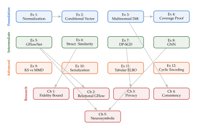
Insight.
The exercises in this section are designed to build intuition from the ground up. Exercises 1–4 focus on the preprocessing and training innovations that made modern tabular generation possible: mode-specific normalization, conditional vectors, discrete diffusion, and coverage guarantees. Exercises 5–8 explore the structural and algorithmic foundations: GFlowNets, dependency graphs, privacy budgets, and graph neural networks. Exercises 9–12 develop evaluation and representation skills: statistical metrics, serialization strategies, variational inference, and cyclic encoding. Together, they cover the complete pipeline from data preprocessing through model design to evaluation.
The challenges are qualitatively different. Each one sits at the intersection of two or more active research areas, requiring not just technical skill but creative synthesis. A complete solution to any single challenge would likely constitute a publishable contribution. Students are encouraged to attempt at least the first parts of each challenge, even if a full solution remains elusive – the act of precisely formulating an open problem is itself a valuable research skill.
Remark 52 (A Note on the Challenges).
The five challenges above are intentionally open-ended. Each represents a genuine research direction at the frontier of structured data generation. Challenge 1 connects evaluation theory to practice; Challenge 2 extends the GFlowNet paradigm to a new domain; Challenge 3 provides foundational privacy analysis for conditional architectures; Challenge 4 bridges consistency models and mixed-type data; and Challenge 5 tackles the largely unexplored problem of automatic constraint discovery. A strong solution to any one of these would constitute a meaningful contribution to the field.
We have now completed our journey through the mathematics of generative models for structured data. From the humble beginnings of applying image-oriented GANs to tabular data, through the careful engineering of preprocessing pipelines and conditional training, to the diverse landscape of diffusion, graph, flow, and language model approaches, we have seen a field mature rapidly. The exercises above provide entry points for further exploration. The challenges point toward the open frontier. The mathematical tools are in your hands – what you build with them is up to you.
References
-
Statistical Disclosure Limitation
BibTeX
@book{rubin1993statistical, title = {Statistical Disclosure Limitation}, author = {Rubin, Donald B.}, journal = {Journal of Official Statistics}, volume = {9}, number = {2}, pages = {461--468}, year = {1993} }Book
-
Harpoon: Manifold-Guided Diffusion for Tabular Data
BibTeX
@article{liu2024harpoon, title = {Harpoon: Manifold-Guided Diffusion for Tabular Data}, author = {Liu, Tennison and Lipkova, Jana and van der Schaar, Mihaela}, journal = {arXiv preprint arXiv:2401.14726}, year = {2024} }Journal article
-
PrivBayes: Private Data Release via Bayesian Networks
BibTeX
@article{zhang2017privbayes, title = {{PrivBayes}: Private Data Release via {Bayesian} Networks}, author = {Zhang, Jun and Cormode, Graham and Procopiuc, Cecilia M. and Srivastava, Divesh and Xiao, Xiaokui}, journal = {ACM Transactions on Database Systems}, volume = {42}, number = {4}, pages = {1--41}, year = {2017} }Journal article
-
Modeling Tabular Data Using Conditional GAN
BibTeX
@article{xu2019modeling, title = {Modeling Tabular Data Using Conditional {GAN}}, author = {Xu, Lei and Skoularidou, Maria and Cuesta-Infante, Alfredo and Veeramachaneni, Kalyan}, journal = {Advances in Neural Information Processing Systems}, volume = {32}, year = {2019} }Journal article
-
CTAB-GAN+: Enhancing Tabular Data Synthesis
BibTeX
@inproceedings{zhao2021ctabganplus, title = {{CTAB-GAN+}: Enhancing Tabular Data Synthesis}, author = {Zhao, Zilong and Kunar, Aditya and Birke, Robert and Chen, Lydia Y.}, booktitle = {Frontiers in Big Data}, year = {2023} }Conference paper
-
TabDDPM: Modelling Tabular Data with Diffusion Models
BibTeX
@inproceedings{kotelnikov2023tabddpm, author = {Kotelnikov, Akim and Baranchuk, Dmitry and Rubachev, Ivan and Babenko, Artem}, title = {{TabDDPM}: Modelling Tabular Data with Diffusion Models}, booktitle = {Proceedings of ICML}, year = {2023} }Conference paper
-
GOGGLE: Generative Modelling for Tabular Data by Learning Relational Structure
BibTeX
@inproceedings{liu2023goggle, author = {Liu, Tennison and Kolossov, Zhaozhi and Yoon, Jinsung and Mihaela van der Schaar}, title = {{GOGGLE}: Generative Modelling for Tabular Data by Learning Relational Structure}, booktitle = {Proceedings of ICLR}, year = {2023} }Conference paper
-
Conditional Generative Adversarial Nets
BibTeX
@misc{mirza2014conditional, title={Conditional Generative Adversarial Nets}, author={Mehdi Mirza and Simon Osindero}, year={2014}, eprint={1411.1784}, archivePrefix={arXiv}, primaryClass={cs.LG} }Reference
-
Categorical Reparameterization with Gumbel-Softmax
BibTeX
@inproceedings{jang2017categorical, title={Categorical Reparameterization with {G}umbel-Softmax}, author={Jang, Eric and Gu, Shixiang and Poole, Ben}, booktitle={International Conference on Learning Representations (ICLR)}, year={2017} }Conference paper
-
Pacgan: The power of two samples in generative adversarial networks
BibTeX
@inproceedings{lin2018pacgan, title={Pacgan: The power of two samples in generative adversarial networks}, author={Lin, Zinan and Khetarpal, Ashish and Fanti, Giulia and Oh, Sewoong}, booktitle={Advances in Neural Information Processing Systems}, pages={1498--1507}, year={2018} }Conference paper
-
Improved training of Wasserstein GANs
BibTeX
@inproceedings{gulrajani2017improved, title={Improved training of Wasserstein GANs}, author={Gulrajani, Ishaan and Ahmed, Faruk and Arjovsky, Martin and Dumoulin, Vincent and Courville, Aaron C}, booktitle={Advances in neural information processing systems}, pages={5767--5777}, year={2017} }Conference paper
-
Wasserstein GAN
BibTeX
@article{arjovsky2017wasserstein, title = {Wasserstein GAN}, author = {Arjovsky, Martin and Chintala, Soumith and Bottou, L\'eon}, journal = {arXiv:1701.07875}, year = {2017} }Journal article
-
On the Regularization of Wasserstein GANs
BibTeX
@article{petzka2018regularization, title = {On the Regularization of {Wasserstein} {GANs}}, author = {Petzka, Henning and Fischer, Asja and Lukovnikov, Denis}, journal = {arXiv preprint arXiv:1709.08894}, year = {2018} }Journal article
-
CTAB-GAN: Effective Table Data Synthesizing
BibTeX
@inproceedings{zhao2021ctabgan, title = {{CTAB-GAN}: Effective Table Data Synthesizing}, author = {Zhao, Zilong and Kunar, Aditya and Birke, Robert and Chen, Lydia Y.}, booktitle = {Asian Conference on Machine Learning}, year = {2021} }Conference paper
-
Unsupervised Representation Learning with Deep Convolutional Generative Adversarial Networks
BibTeX
@inproceedings{radford2016unsupervised, title = {Unsupervised Representation Learning with Deep Convolutional Generative Adversarial Networks}, author = {Radford, Alec and Metz, Luke and Chintala, Soumith}, booktitle = {International Conference on Learning Representations}, year = {2016} }Conference paper
-
Conditional Image Synthesis With Auxiliary Classifier GANs
BibTeX
@article{odena2017conditional, title = {Conditional Image Synthesis With Auxiliary Classifier {GANs}}, author = {Odena, Augustus and Olah, Christopher and Shlens, Jonathon}, journal = {Proceedings of the International Conference on Machine Learning}, year = {2017} }Journal article
-
Deep Learning with Differential Privacy
BibTeX
@inproceedings{abadi2016deep, title={Deep Learning with Differential Privacy}, author={Abadi, Martin and Chu, Andy and Goodfellow, Ian and McMahan, H Brendan and Mironov, Ilya and Talwar, Kunal and Zhang, Li}, booktitle={ACM SIGSAC Conference on Computer and Communications Security (CCS)}, pages={308--318}, year={2016}, publisher={ACM} }Conference paper
-
The Privacy Blanket of the Shuffle Model
BibTeX
@article{balle2018privacy, title = {The Privacy Blanket of the Shuffle Model}, author = {Ball{\'e}, Borja and Barthe, Gilles and Gavin, Marco}, journal = {arXiv preprint arXiv:1802.10025}, year = {2018} }Journal article
-
The Algorithmic Foundations of Differential Privacy
BibTeX
@book{dwork2014algorithmic, title = {The Algorithmic Foundations of Differential Privacy}, author = {Dwork, Cynthia and Roth, Aaron}, publisher = {Foundations and Trends in Theoretical Computer Science}, volume = {9}, number = {3--4}, pages = {211--407}, year = {2014} }Book
-
Fake It Till You Make It: Guidelines for Effective Synthetic Data Generation
BibTeX
@article{dankar2021fake, title = {Fake It Till You Make It: Guidelines for Effective Synthetic Data Generation}, author = {Dankar, Fida K. and Ibrahim, Mariam}, journal = {Applied Sciences}, volume = {11}, number = {5}, pages = {2158}, year = {2021} }Journal article
-
DeepInsight: A methodology to transform a non-image data to an image for convolution neural network architecture
BibTeX
@article{sharma2019deepinsight, title = {{DeepInsight}: A methodology to transform a non-image data to an image for convolution neural network architecture}, author = {Sharma, Alok and Vans, Edwin and Karamouzian, Daichi and Tsunoda, Tatsuhiko}, journal = {Scientific Reports}, volume = {9}, pages = {11399}, year = {2019} }Journal article
-
-VAE: Learning Basic Visual Concepts with a Constrained Variational Framework
BibTeX
@inproceedings{higgins2017beta, title={$\beta$-{VAE}: Learning Basic Visual Concepts with a Constrained Variational Framework}, author={Higgins, Irina and Matthey, Loic and Pal, Arka and Burgess, Christopher and Glorot, Xavier and Botvinick, Matthew and Mohamed, Shakir and Lerchner, Alexander}, booktitle={International Conference on Learning Representations}, year={2017} }Conference paper
-
Denoising Diffusion Implicit Models
BibTeX
@article{song2021denoising, title = {Denoising Diffusion Implicit Models}, author = {Song, Jiaming and Meng, Chenlin and Ermon, Stefano}, journal = {arXiv preprint arXiv:2010.02502}, year = {2021} }Journal article
-
Denoising Diffusion Probabilistic Models
BibTeX
@inproceedings{ho2020denoising, title={Denoising Diffusion Probabilistic Models}, author={Ho, Jonathan and Jain, Ajay and Abbeel, Pieter}, booktitle={Advances in Neural Information Processing Systems}, volume={33}, pages={6840--6851}, year={2020} }Conference paper
-
TabuLa: Harnessing Language Models for Tabular Data Synthesis
BibTeX
@inproceedings{zhao2023tabula, author = {Zhao, Zilong and Birke, Robert and Chen, Lydia Y.}, title = {{TabuLa}: Harnessing Language Models for Tabular Data Synthesis}, booktitle = {NeurIPS Workshop on Table Representation Learning}, year = {2023} }Conference paper
-
An Explanation of In-Context Learning as Implicit Bayesian Inference
BibTeX
@inproceedings{xie2022explanation, title={An Explanation of In-Context Learning as Implicit {Bayesian} Inference}, author={Xie, Sang Michael and Raghunathan, Aditi and Liang, Percy and Ma, Tengyu}, booktitle={Proceedings of the International Conference on Learning Representations (ICLR)}, year={2022} }Conference paper
-
Language Models are Realistic Tabular Data Generators
BibTeX
@article{borisov2023language, title = {Language Models are Realistic Tabular Data Generators}, author = {Borisov, Vadim and Seßler, Kathrin and Leemann, Tobias and Pawelczyk, Martin and Kasneci, Gjir}, journal = {arXiv preprint arXiv:2210.06280}, year = {2023} }Journal article
-
Extracting Training Data from Large Language Models
BibTeX
@inproceedings{carlini2021extracting, title={Extracting Training Data from Large Language Models}, author={Carlini, Nicholas and Tramer, Florian and Wallace, Eric and Jagielski, Matthew and Herbert-Voss, Ariel and Lee, Katherine and Roberts, Adam and Brown, Tom and Song, Dawn and Erlingsson, Ulfar and Oprea, Alina and Raffel, Colin}, booktitle={USENIX Security Symposium}, pages={2633--2650}, year={2021} }Conference paper
-
A Kernel Two-Sample Test
BibTeX
@article{gretton2012mmd, author = {Gretton, Arthur and Borgwardt, Karsten M. and Rasch, Malte J. and Sch{\"o}lkopf, Bernhard and Smola, Alexander}, title = {A Kernel Two-Sample Test}, journal = {Journal of Machine Learning Research}, volume = {13}, pages = {723--773}, year = {2012} }Journal article
-
Random Features for Large-Scale Kernel Machines
BibTeX
@inproceedings{rahimi2007random, title = {Random Features for Large-Scale Kernel Machines}, author = {Rahimi, Ali and Recht, Benjamin}, booktitle = {Advances in Neural Information Processing Systems}, volume = {20}, year = {2007} }Conference paper
-
Modeling Tabular Data using Conditional GAN
BibTeX
@inproceedings{xu2019ctgan, author = {Xu, Lei and Skoularidou, Maria and Cuesta-Infante, Alfredo and Veeramachaneni, Kalyan}, title = {Modeling Tabular Data using Conditional {GAN}}, booktitle = {Advances in Neural Information Processing Systems (NeurIPS)}, year = {2019} }Conference paper
-
CTAB-GAN+: Enhancing Tabular Data Synthesis
BibTeX
@article{zhao2024ctabganplus, author = {Zhao, Zilong and Kunar, Aditya and Birke, Robert and Chen, Lydia Y.}, title = {{CTAB-GAN+}: Enhancing Tabular Data Synthesis}, journal = {Frontiers in Big Data}, volume = {7}, year = {2024} }Journal article
-
Generative Adversarial Networks
BibTeX
@inproceedings{goodfellow2014generative, title={Generative Adversarial Networks}, author={Goodfellow, Ian and Pouget-Abadie, Jean and Mirza, Mehdi and Xu, Bing and Warde-Farley, David and Ozair, Sherjil and Courville, Aaron and Bengio, Yoshua}, booktitle={Advances in Neural Information Processing Systems}, volume={27}, year={2014} }Conference paper
-
Generating Multi-label Discrete Patient Records using Generative Adversarial Networks
BibTeX
@article{choi2017generating, title={Generating Multi-label Discrete Patient Records using Generative Adversarial Networks}, author={Choi, Edward and Biswal, Siddharth and Malin, Bradley and Duke, Jon and Stewart, Walter F and Sun, Jimeng}, journal={arXiv preprint arXiv:1703.06490}, year={2017} }Journal article
-
Flow Network Based Generative Models for Non-Iterative Diverse Candidate Generation
BibTeX
@article{bengio2021flow, title = {Flow Network Based Generative Models for Non-Iterative Diverse Candidate Generation}, author = {Bengio, Emmanuel and Jain, Moksh and Korablyov, Maksym and Precup, Doina and Bengio, Yoshua}, journal = {Advances in Neural Information Processing Systems}, volume = {34}, year = {2021} }Journal article
-
The EU General Data Protection Regulation (GDPR)
BibTeX
@misc{voigt2017gdpr, title = {The {EU} General Data Protection Regulation ({GDPR})}, author = {Voigt, Paul and von dem Bussche, Axel}, publisher = {Springer}, year = {2017} }Reference
-
k-Anonymity: A Model for Protecting Privacy
BibTeX
@article{sweeney2002kanonymity, title = {k-Anonymity: A Model for Protecting Privacy}, author = {Sweeney, Latanya}, journal = {International Journal of Uncertainty, Fuzziness and Knowledge-Based Systems}, volume = {10}, number = {5}, pages = {557--570}, year = {2002} }Journal article
-
A Style-Based Generator Architecture for Generative Adversarial Networks
BibTeX
@misc{karras2019stylebased, title={A Style-Based Generator Architecture for Generative Adversarial Networks}, author={Tero Karras and Samuli Laine and Timo Aila}, year={2019}, eprint={1812.04948}, archivePrefix={arXiv}, primaryClass={cs.NE} }Reference
-
Language Models are Few-Shot Learners
BibTeX
@article{brown2020language, title={Language Models are Few-Shot Learners}, author={Brown, Tom B and Mann, Benjamin and Ryder, Nick and Subbiah, Melanie and Kaplan, Jared and Dhariwal, Prafulla and Neelakantan, Arvind and Shyam, Pranav and Sastry, Girish and Askell, Amanda and others}, year={2020} }Journal article
-
Gans trained by a two time-scale update rule converge to a local nash equilibrium
BibTeX
@inproceedings{heusel2017gans, title={Gans trained by a two time-scale update rule converge to a local nash equilibrium}, author={Heusel, Martin and Ramsauer, Hubertus and Unterthiner, Thomas and Nessler, Bernhard and Hochreiter, Sepp}, booktitle={Advances in Neural Information Processing Systems}, pages={6626--6637}, year={2017} }Conference paper
-
Calibrating Noise to Sensitivity in Private Data Analysis
BibTeX
@inproceedings{dwork2006calibrating, title={Calibrating Noise to Sensitivity in Private Data Analysis}, author={Dwork, Cynthia and McSherry, Frank and Nissim, Kobbi and Smith, Adam}, booktitle={Theory of Cryptography Conference (TCC)}, pages={265--284}, year={2006}, publisher={Springer} }Conference paper
-
CTAB-GAN+: Enhancing Tabular Data Synthesis
BibTeX
@article{zhao2022ctabganp, title = {{CTAB-GAN+}: Enhancing Tabular Data Synthesis}, author = {Zhao, Zilong and Kunar, Aditya and Birke, Robert and Chen, Lydia Y.}, journal = {Frontiers in Big Data}, volume = {6}, year = {2023} }Journal article
-
Argmax Flows and Multinomial Diffusion
BibTeX
@article{hoogeboom2021argmax, author = {Hoogeboom, Emiel and Nielsen, Didrik and Jaini, Priyank and Forr{\'e}, Patrick and Welling, Max}, title = {Argmax Flows and Multinomial Diffusion}, journal = {Proceedings of ICML}, year = {2021} }Journal article
-
Harpoon: Conditional Tabular Generation with Manifold Guidance
BibTeX
@inproceedings{liu2025harpoon, author = {Liu, Tennison and Seedat, Nabeel and Imrie, Fergus and van der Schaar, Mihaela}, title = {Harpoon: Conditional Tabular Generation with Manifold Guidance}, booktitle = {Proceedings of ICLR}, year = {2025} }Conference paper
-
Score-Based Generative Modeling through Stochastic Differential Equations
BibTeX
@article{song2021scorebased, author = {Song, Yang and Sohl-Dickstein, Jascha and Kingma, Diederik P. and Kumar, Abhishek and Ermon, Stefano and Poole, Ben}, title = {Score-Based Generative Modeling through Stochastic Differential Equations}, journal = {Proceedings of ICLR}, year = {2021} }Journal article
-
Diffusion Models Beat GANs on Image Synthesis
BibTeX
@inproceedings{dhariwal2021diffusion, title = {Diffusion Models Beat {GANs} on Image Synthesis}, author = {Dhariwal, Prafulla and Nichol, Alexander}, booktitle = {Advances in Neural Information Processing Systems}, volume = {34}, year = {2021} }Conference paper
-
WaveStitch: Pipelined-Parallel Synthetic Time Series Generation
BibTeX
@article{wavestitch2024, author = {Li, Zhenyu and others}, title = {{WaveStitch}: Pipelined-Parallel Synthetic Time Series Generation}, journal = {arXiv preprint arXiv:2410.XXXXX}, year = {2024}, note = {Pipelined-parallel approach to long time-series generation} }Journal article
-
Chronos: Learning the Language of Time Series
BibTeX
@article{ansari2024wavestitch, author = {Ansari, Abdul Fatir and Stella, Lorenzo and Turkmen, Caner and Zhang, Xiyuan and Mercado, Pedro and Shen, Huibin and Shchur, Oleksandr and Rangapuram, Syama Sundar and Arber Pineda, Sebastian and Gasthaus, Jan and Wang, Yuyang and Januschowski, Tim}, title = {Chronos: Learning the Language of Time Series}, journal = {Transactions on Machine Learning Research}, year = {2024}, note = {WaveStitch uses Chronos-style ideas for time-series stitching} }Journal article
-
LLaMA: Open and Efficient Foundation Language Models
BibTeX
@article{touvron2023llama, author = {Touvron, Hugo and Lavril, Thibaut and Izacard, Gautier and Martinet, Xavier and Lachaux, Marie-Anne and others}, title = {{LLaMA}: Open and Efficient Foundation Language Models}, journal = {arXiv preprint arXiv:2302.13971}, year = {2023} }Journal article
-
XLNet: Generalized autoregressive pretraining for language understanding
BibTeX
@article{yang2019xlnet, title={{XLNet}: Generalized autoregressive pretraining for language understanding}, author={Yang, Zhilin and Dai, Zihang and Yang, Yiming and Carbonell, Jaime and Salakhutdinov, Ruslan R and Le, Quoc V}, journal={Advances in Neural Information Processing Systems}, volume={32}, year={2019} }Journal article
-
Outrageously Large Neural Networks: The Sparsely-Gated Mixture-of-Experts Layer
BibTeX
@inproceedings{shazeer2017outrageously, title={Outrageously Large Neural Networks: The Sparsely-Gated Mixture-of-Experts Layer}, author={Shazeer, Noam and Mirhoseini, Azalia and Maziarz, Krzysztof and Davis, Andy and Le, Quoc and Hinton, Geoffrey and Dean, Jeff}, booktitle={International Conference on Learning Representations}, year={2017} }Conference paper
-
Mixtral of Experts
BibTeX
@misc{jiang2024mixtral, title={Mixtral of Experts}, author={Jiang, Albert Q. and Sablayrolles, Alexandre and Roux, Antoine and Mensch, Arthur and Savary, Blanche and Bamford, Chris and Chaplot, Devendra Singh and de las Casas, Diego and Hanna, Emma Bou and Bressand, Florian and others}, year={2024}, eprint={2401.04088}, archiveprefix={arXiv}, primaryclass={cs.LG} }Reference
-
Switch Transformers: Scaling to Trillion Parameter Models with Simple and Efficient Sparsity
BibTeX
@article{fedus2022switch, title={Switch Transformers: Scaling to Trillion Parameter Models with Simple and Efficient Sparsity}, author={Fedus, William and Zoph, Barret and Shazeer, Noam}, journal={Journal of Machine Learning Research}, volume={23}, number={120}, pages={1--39}, year={2022} }Journal article
-
TabStruct: Evaluating Structural Fidelity of Synthetic Tabular Data
BibTeX
@article{liu2025tabstruct, author = {Liu, Tennison and Kolossov, Zhaozhi and Yoon, Jinsung and van der Schaar, Mihaela}, title = {{TabStruct}: Evaluating Structural Fidelity of Synthetic Tabular Data}, journal = {Proceedings of AAAI}, year = {2025} }Journal article
-
Flow Network based Generative Models for Non-Iterative Diverse Candidate Generation
BibTeX
@inproceedings{bengio2021gflownet, author = {Bengio, Emmanuel and Jain, Moksh and Korablyov, Maksym and Precup, Doina and Bengio, Yoshua}, title = {Flow Network based Generative Models for Non-Iterative Diverse Candidate Generation}, booktitle = {Advances in Neural Information Processing Systems (NeurIPS)}, year = {2021} }Conference paper
-
GFlowNet Foundations
BibTeX
@article{bengio2023gflownet, title = {{GFlowNet} Foundations}, author = {Bengio, Yoshua and Lahlou, Salem and Deleu, Tristan and Hu, Edward J. and Tiwari, Mo and Bengio, Emmanuel}, journal = {Journal of Machine Learning Research}, volume = {24}, number = {210}, pages = {1--55}, year = {2023} }Journal article
-
Trajectory Balance: Improved Credit Assignment in GFlowNets
BibTeX
@article{malkin2022trajectory, title = {Trajectory Balance: Improved Credit Assignment in {GFlowNets}}, author = {Malkin, Nikolay and Jain, Moksh and Bengio, Emmanuel and Sun, Chen and Bengio, Yoshua}, journal = {Advances in Neural Information Processing Systems}, volume = {35}, year = {2022} }Journal article
-
Consistency Models
BibTeX
@article{song2023consistency, title={Consistency Models}, author={Song, Yang and Dhariwal, Prafulla and Chen, Mark and Sutskever, Ilya}, journal={International Conference on Machine Learning}, year={2023} }Journal article