32 Generative Models in Retrieval: From Memory to Meaning
The Philosophy of Retrieval – What Does It Mean to Remember?
You have lost your keys. You stand in the hallway, pockets empty, mind racing. Where did you last see them? You close your eyes. An image surfaces – the kitchen counter, the morning light, a coffee cup beside a set of keys. You walk to the kitchen. There they are.
What just happened? On the surface, a trivial act of memory. Beneath the surface, one of the most profound computational processes known to science. Your brain, without being told where to look, without scanning every object in the house, without any external index or catalogue, reconstructed a scene from partial cues, identified the relevant fragment, and translated that fragment into an action. It did not search for the keys in any mechanical sense. It remembered them – which is to say, it generated a plausible past from compressed traces of experience.
This chapter is about retrieval – the problem of finding relevant information given a need. But we begin with a confession: the word “retrieval” is misleading. It suggests a filing cabinet, a librarian pulling a book from a shelf, a database returning a row. These metaphors imply that the information exists somewhere in its original form, waiting to be fetched. The truth, as neuroscience and modern generative AI reveal, is far stranger. What we call retrieval is often closer to reconstruction, to generation, to the creative act of assembling meaning from fragments. Understanding this distinction – between retrieval as lookup and retrieval as generation – is the central theme of everything that follows.
Plato's Anamnesis: All Learning Is Recollection
Twenty-four centuries ago, Plato proposed a theory of knowledge that sounds, to modern ears, both mystical and eerily prescient. In the Meno dialogue, Socrates demonstrates that an uneducated slave boy can derive geometric truths when prompted with the right questions. Socrates' conclusion is startling: the boy did not learn these truths; he remembered them. The soul, Plato argues, has encountered all truths in a prior existence; what we call learning is merely anamnesis – recollection of what we already know.
Strip away the metaphysics, and Plato's insight contains a kernel that resonates with modern retrieval systems. The idea that knowledge is not acquired but recovered – that the answer to a question already exists, latent, in some compressed form, and the task is to surface it – is precisely what happens when a large language model answers a query. The model does not search an external database. It reaches into its parameters, into the compressed traces of billions of documents encountered during training, and reconstructs an answer. The parameters are the model's soul; inference is its anamnesis.
Remark 1.
Plato's anamnesis is not merely a historical curiosity. It foreshadows the distinction between retrieval-based and parametric knowledge systems that dominates modern NLP. A retrieval-based system consults an external corpus at query time. A parametric system (such as a language model) stores knowledge implicitly in its weights. The tension between these paradigms – and their eventual synthesis in retrieval-augmented generation – is a central arc of this chapter.
Aristotle's Associations: Similarity, Contiguity, Contrast
Where Plato looked upward to transcendent Forms, his student Aristotle looked around at the empirical world. In De Memoria et Reminiscentia (On Memory and Reminiscence), Aristotle proposed that memories are retrieved through three principles of association:
Similarity. We recall things that resemble the current stimulus. The smell of cinnamon recalls your grandmother's kitchen. In computational terms, this is nearest-neighbour search in a feature space.
Contiguity. We recall things that occurred together in space or time. The sight of a lecture hall recalls a specific class. This is co-occurrence statistics, the foundation of methods from TF-IDF to word embeddings [1].
Contrast. We recall things that are opposite to the current stimulus. The word “hot” triggers “cold.” This is negative sampling, the mechanism by which modern embedding methods learn discriminative representations.
It is remarkable how directly these twenty-three-century-old principles map onto the core mechanisms of modern information retrieval. Similarity retrieval is the foundation of vector search. Contiguity is exploited by language models that learn from co-occurrence patterns. Contrast is the training signal in contrastive learning and hard negative mining. Aristotle did not have matrices, but he had the right intuitions.
Borges' Library of Babel: The Retrieval Problem
In 1941, Jorge Luis Borges published a short story that is, arguably, the most profound meditation on the retrieval problem ever written. “The Library of Babel” describes a universe consisting of an enormous library containing every possible book of a fixed length – every possible arrangement of twenty-five characters across 410 pages. The library contains every truth ever uttered and every truth yet to be discovered. It contains the complete works of Shakespeare, the cure for cancer, the biography of every person who will ever live. It also contains every possible variation of these texts with a single character changed, and every text that is pure gibberish.
The inhabitants of the library are driven mad. Not because the knowledge is unavailable – it is all there, every last word of it – but because they cannot find it. The ratio of meaningful books to meaningless ones is vanishingly small; a librarian could wander the hexagonal galleries for a lifetime without finding a single coherent sentence. Storage is solved. Retrieval is impossible.
Key Idea.
The Borges Principle: Storage Without Retrieval Is Meaningless. The Library of Babel teaches us that the fundamental problem of information systems is not how much we can store, but how well we can retrieve. A petabyte database without an effective retrieval mechanism is no more useful than Borges' infinite library. This insight motivates the entire field of information retrieval: the challenge is not in having answers, but in connecting questions to answers.
The modern internet is eerily close to Borges' vision. As of 2024, the indexed web contains hundreds of billions of pages. The vast majority are irrelevant to any given query. Google's PageRank algorithm, the neural retrieval models we shall study in later sections, and the retrieval-augmented generation pipelines that power modern AI assistants are all, in essence, solutions to the Library of Babel problem: mechanisms for finding the needle of relevance in the haystack of all possible texts.
Wittgenstein and the Contextuality of Meaning
There is a deeper problem that Borges' library does not address. Even if we could find the right book, would we know it was the right one? Relevance is not a property of documents in isolation; it depends on the query, the querier, the context, and the purpose.
Ludwig Wittgenstein, in his Philosophical Investigations (1953), argued that the meaning of a word is not some fixed, Platonic entity but its use in a language game – the social, contextual, practical circumstances in which it is employed. The word “bank” means one thing to a fisherman and another to a financier. The query “How to deal with depression” means one thing to a psychologist and another to a meteorologist studying atmospheric pressure systems.
Wittgenstein's insight cuts at the heart of a fundamental limitation of early retrieval systems. Term-matching approaches like TF-IDF [5] treat queries and documents as bags of tokens, ignoring the vast web of contextual meaning that determines relevance. A query for “jaguar speed” could seek information about the animal, the car, or the Atari game. The string is identical; the meaning is determined entirely by context.
This is why the transition from lexical retrieval (matching words) to semantic retrieval (matching meanings) represents one of the most important revolutions in the history of the field. Dense retrieval models – which embed queries and documents into a shared vector space where distance reflects semantic similarity rather than lexical overlap – are the computational realisation of Wittgenstein's philosophy. They encode not strings, but uses, not words, but meanings in context.
Insight.
Retrieval Is Not String Matching; It Is Meaning Matching. The evolution from lexical to semantic retrieval recapitulates, in the history of computer science, the philosophical journey from Plato's fixed Forms to Wittgenstein's contextual language games. Each word, each query, each document is a node in a vast network of usage, and its meaning is determined by its position in that network. Modern dense retrieval models learn precisely this network structure from data.
The Formal Retrieval Problem
Having gathered philosophical motivation, we now make the retrieval problem precise. Every retrieval system, from the ancient librarian of Alexandria to GPT-4's retrieval-augmented generation pipeline, can be understood as an instance of the following formalism.
Definition 1 (The Retrieval Problem).
Let be a query space and be a document space (or, more generally, an item space). Let be a relevance function, where if and only if document is relevant to query . The retrieval problem is: given a query and a corpus , produce a ranked list such that relevant documents appear before irrelevant ones.
Formally, we seek a scoring function such that the induced ranking , defined by for all , maximises some evaluation metric (e.g., average precision, nDCG) with respect to : (Retrieval Objective) where is a family of scoring functions and is the distribution over queries.
Example 1.
In web search, is the set of all possible text queries, is the set of all web pages, is determined by human relevance judgments (e.g., TREC assessors [2]), and the scoring function is a complex pipeline combining BM25, neural rankers, click models, and personalisation signals. The metric is typically nDCG [3].
Example 2.
In human memory recall, is the set of all possible cues (a smell, a sound, a question on an exam), is the set of all encoded memories, is determined by relevance to the current cognitive task, and is the unconscious pattern-completion process implemented by hippocampal–cortical circuits. Evolution has optimised over millions of years.
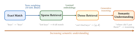
The retrieval spectrum shown in Figure 1 illustrates the central trajectory of this chapter. We begin with exact match – the simplest and oldest form of retrieval – and progress through sparse methods, dense methods, and finally generative retrieval, where the system does not merely find relevant documents but generates answers, identifiers, or entirely new text that synthesises information from multiple sources.
Retrieval as Reconstruction
We arrive at the central philosophical claim of this chapter, the thread that will weave through every section that follows.
Key Idea.
Retrieval Is Not Lookup; It Is Reconstruction. Classical retrieval systems treat the corpus as a static archive and the retrieval process as a lookup operation: find the document that matches the query. Generative retrieval systems invert this paradigm. They compress the corpus into the parameters of a neural network and, at query time, reconstruct the answer – or the document identifier, or the passage – from this compressed representation. In this view, retrieval and generation are not opposites but two facets of the same process: the recovery of meaning from compressed memory.
This reconstruction view unifies several threads that have traditionally been studied in isolation. Autoregressive language models that answer questions from their parameters are performing retrieval by generation. Retrieval-augmented generation systems that condition on retrieved passages are performing generation by retrieval. The boundary between the two dissolves once we recognise that both are instances of the same fundamental operation: reconstructing relevant information from a combination of parametric memory (weights) and non-parametric memory (the corpus).
Historical Note.
The Library of Alexandria: Humanity's First Retrieval Crisis. The Great Library of Alexandria, founded around 283 BCE under Ptolemy II, was the ancient world's most ambitious attempt to collect all human knowledge. At its peak, it held an estimated 400,000 to 700,000 scrolls. But as the collection grew, a crisis emerged that will sound familiar to any modern information scientist: how to find anything.
The solution came from the poet and scholar Callimachus, who created the Pinakes – a 120-volume catalogue that organised the library's holdings by genre (rhetoric, law, epic poetry, tragedy, comedy, lyric poetry, history, medicine, mathematics, natural science, miscellaneous) and within each genre, alphabetically by author. The Pinakes was, in effect, the world's first inverted index.
The lesson of Alexandria is that the problem of retrieval is as old as the problem of knowledge itself. Every information explosion – from the invention of writing, to the printing press, to the internet – creates a retrieval crisis that demands new organisational principles. We are living through such a crisis now, and generative models are the latest attempt at a solution.
Exercise 1.
Consider a simplified Library of Babel containing all possible strings of length over an alphabet of size .
How many books does the library contain?
If a “meaningful” book is one whose characters form valid English with probability at least under a language model , estimate the fraction of meaningful books as a function of , , and the per-character entropy of English (approximately 1.3 bits per character, per Shannon [4]).
Argue that as , the retrieval problem in Borges' library becomes arbitrarily hard under any uniform scanning strategy, but remains tractable if one has access to a good language model as an oracle.
Exercise 2.
Plato's theory of anamnesis claims that learning is recollection. A large language model stores knowledge in its parameters and “recollects” it at inference time.
In what precise sense is a forward pass through a language model analogous to Platonic recollection? Identify the analogue of the “prior existence” where knowledge was acquired.
What is the key disanalogy? (Hint: consider hallucination.)
Propose a formal test to distinguish whether a model is “retrieving” a memorised training passage or “generating” a novel synthesis.
Exercise 3.
Wittgenstein argued that meaning depends on context.
Give three queries where the same words have completely different retrieval intents depending on the user's context.
For each query, describe how a dense retrieval model with access to user context could resolve the ambiguity.
Formalise the notion of “context-dependent relevance” by extending Definition 1 to include a context variable .
Exercise 4.
Place the following systems on the retrieval spectrum of
Figure 1: (a) grep, (b) Google
circa 2004, (c) a BERT cross-encoder reranker, (d) ChatGPT
answering from parametric memory, (e) a retrieval-augmented
generation system. Justify each placement.
Exercise 5.
The claim that “retrieval is reconstruction” has testable consequences.
Describe an experiment that would distinguish between a retrieval system that performs pure lookup (returns a stored passage verbatim) and one that performs reconstruction (generates a response influenced by, but not identical to, stored data).
Large language models sometimes “hallucinate” – they generate plausible but factually incorrect text. Argue that hallucination is a predictable consequence of the reconstruction view of retrieval.
Propose a metric that quantifies the degree to which a system's output is “retrieved” versus “generated.” (Hint: consider measuring the n-gram overlap with the training corpus.)
The Neuroscience of Memory and Retrieval
If we wish to build machines that retrieve information as fluidly as the human mind, we would do well to understand how the mind itself accomplishes this feat. The brain is, among many other things, the most sophisticated retrieval engine ever constructed – capable of recovering a specific childhood memory from a whiff of perfume, of completing a partial melody from its first three notes, of answering a novel question by synthesising information from decades of experience. How does it do this?
The answer, as we shall see, offers profound lessons for the design of artificial retrieval systems – and reveals that the brain's approach to retrieval is far closer to generation than to lookup.
The Hippocampus as a Retrieval Engine
In 1953, a young man known as patient H.M. underwent bilateral surgical removal of his medial temporal lobes, including most of his hippocampus, as a treatment for severe epilepsy. The seizures stopped, but something else was lost: H.M. could no longer form new long-term memories. He could remember his childhood, carry on a conversation, and solve puzzles, but five minutes after meeting someone, he had no recollection of the encounter [41].
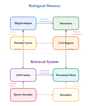
H.M.'s tragedy transformed our understanding of memory. It revealed that the hippocampus is not a passive storage vault but an active indexing and retrieval system – a biological analogue of the very retrieval engines we build in software. The hippocampus performs two critical functions:
Rapid encoding.
The hippocampus can encode new associations in a single exposure – a property called one-shot learning in the machine learning literature. When you meet someone new, your hippocampus rapidly binds together the person's face, name, voice, and the context of the encounter into a unified memory trace. This is achieved through a form of sparse, pattern-separated encoding: the hippocampal dentate gyrus uses highly sparse activity patterns to represent distinct memories, ensuring that similar experiences are stored in non-overlapping representations [35].
Pattern completion.
When a partial cue arrives – a familiar face, a fragment of a song, the smell of rain – the hippocampus performs pattern completion: it takes the partial input, matches it against stored memory traces, and reactivates the full memory, including components that were not present in the cue. You see the face and recall the name, the voice, the restaurant where you met. This is not lookup; it is reconstruction. The hippocampus does not store memories as complete records. It stores indices – compressed pointers that, when activated, trigger the reconstruction of the full memory from distributed cortical representations.
The parallels to modern retrieval systems are striking. The hippocampus is the index; the neocortex is the document store. Pattern completion is approximate nearest-neighbour search – finding the stored representation most similar to the query cue and then expanding it into a full response.
Consider what happens when you try to remember a colleague's name. The cue – perhaps the person's face – arrives at the hippocampus. The hippocampus does not search through every memory trace sequentially (that would be and the brain has billions of traces). Instead, the sparse activity pattern generated by the cue directly activates a small number of candidate memory traces through content-addressable lookup – the biological equivalent of hash-based or graph-based approximate nearest-neighbour search. The best-matching trace “wins” through a competitive process (lateral inhibition in CA3), and the full memory – name, voice, context – is reconstructed from the index pointer.
The computational cost of this biological retrieval is remarkable. The hippocampus achieves sublinear query time through three mechanisms that have direct analogues in computer science: locality-sensitive hashing (through sparse, random projections in the dentate gyrus), winner-take-all competition (through lateral inhibition in CA3), and iterative refinement (through recurrent dynamics that converge to an attractor state). Each of these mechanisms has inspired a family of approximate nearest-neighbour algorithms.
Episodic and Semantic Memory
In 1972, the cognitive psychologist Endel Tulving proposed a distinction that has profoundly shaped our understanding of memory and, by extension, of retrieval [36]. He argued that long-term memory comprises at least two qualitatively different systems:
Episodic memory.
Episodic memory stores specific, personally experienced events, bound to a particular time and place. You remember eating breakfast this morning, your first day of school, the moment you heard a particular piece of news. These memories are rich in contextual detail and are associated with a subjective sense of “re-experiencing” – what Tulving called autonoetic consciousness.
Semantic memory.
Semantic memory stores general knowledge about the world, abstracted from any particular experience. You know that Paris is the capital of France, that water freezes at C, and that mammals are warm-blooded. You do not remember when or where you learned these facts; the knowledge has been separated from its experiential context.
The distinction maps elegantly onto two modes of artificial retrieval:
Passage retrieval is analogous to episodic memory: the system returns specific documents or passages, each tied to a particular source and context. The user “re-experiences” the original text.
Parametric knowledge in a language model is analogous to semantic memory: the model “knows” facts but has lost the connection to the specific training documents from which they were learned. It cannot cite its sources, just as you cannot remember where you learned that .
Insight.
The Brain Does Not Store Memories Like Files. A crucial finding from decades of memory research is that human memories are not stored as fixed, high-fidelity records. They are reconstructed each time they are retrieved, assembled on the fly from distributed fragments, coloured by current emotional state, biased by subsequent experiences, and shaped by the specific retrieval cue. This is why eyewitness testimony is unreliable, why memories of childhood change over a lifetime, and why the act of remembering can itself alter the memory.
Generative retrieval models exhibit exactly this property. A language model does not “look up” a fact from its training data; it generates a response that is influenced by training data but reconstructed in the context of the current query. This is why language models hallucinate: they are doing exactly what human memory does – filling in gaps with plausible confabulations.
Engrams: The Physical Trace of Memory
Where does a memory live? The question haunted neuroscience for a century. In the early 1900s, Richard Semon coined the term engram to denote the physical trace that a memory leaves in the brain – the material substrate of recollection. Karl Lashley spent decades searching for the engram, systematically lesioning rat brains and testing for memory loss. His conclusion, formulated as the “law of mass action,” was that memories are not localised to specific regions but are distributed across the cortex.
The mystery was partially resolved by Susumu Tonegawa's Nobel Prize-winning work, which demonstrated that specific populations of neurons – engram cells – are activated during memory encoding and reactivated during recall [34]. By using optogenetic techniques to artificially activate engram cells in mice, Tonegawa's group could implant false memories – compelling evidence that these cells are indeed the physical substrate of memory.
The engram concept connects directly to the representations learned by neural retrieval models. When a dense retrieval model encodes a document into a vector , that vector is the document's engram – a compressed trace that captures the essential semantic content. When a query vector activates the most similar document vectors through approximate nearest-neighbour search, the system is performing artificial pattern completion, reactivating the “memory” most compatible with the current cue.
Remark 2.
The connection between engrams and embeddings is more than metaphorical. Both are distributed, compressed representations that support content-addressable retrieval. Both exhibit interference (similar memories/documents compete for activation). Both are subject to forgetting (catastrophic forgetting in neural networks; memory decay in biological systems). The parallels suggest that the brain and artificial retrieval systems have converged on similar computational solutions to the same fundamental problem.
Memory Consolidation: From Encoding to Retrieval
A memory is not created in a single instant. The process of transforming an experience into a retrievable memory involves three distinct stages, each with a computational analogue:
Encoding. The experience is perceived and processed by sensory cortices, then rapidly bound into a coherent memory trace by the hippocampus. Computational analogue: the document encoder that maps raw text to a dense embedding vector.
Storage (Consolidation). Over hours to weeks, the hippocampal memory trace is gradually transferred to the neocortex through a process of replay – during sleep, the hippocampus reactivates recent memories, and the neocortex slowly integrates them into its long-term representations. Computational analogue: the indexing phase, where document embeddings are organised into data structures (inverted indices, HNSW graphs, product quantisation codebooks) that support efficient retrieval.
Retrieval. A cue activates the hippocampal index, which triggers pattern completion and reactivates the relevant cortical representations. Computational analogue: the query processing phase, where the query embedding is compared against indexed document embeddings to produce a ranked list of results.
The consolidation stage is particularly illuminating. The brain does not simply dump memories into long-term storage; it replays them, extracting regularities, building abstractions, and gradually transforming episodic memories into semantic knowledge. During slow-wave sleep, the hippocampus replays the day's experiences at compressed timescales (up to 20 times faster than real time), broadcasting them to the neocortex, which gradually integrates the new information into its existing knowledge structures. Over weeks and months, a memory that was once hippocampal-dependent – vivid, contextual, episodic – becomes cortical – abstract, decontextualised, semantic.
This process bears a remarkable resemblance to the distillation and fine-tuning procedures used to train generative retrieval models, where a large corpus is gradually compressed into the parameters of a neural network through repeated exposure during training. The training loop of a neural retrieval model is, computationally speaking, a form of artificial memory consolidation: raw data (experiences) are replayed (iterated over in training epochs) and gradually compressed into the model's parameters (long-term cortical representations).
Remark 3.
The parallel between sleep replay and training epochs is not merely poetic. Kumaran et al. (2016) showed that artificial neural networks trained with interleaved replay of old examples – mimicking hippocampal replay during sleep – exhibit less catastrophic forgetting than networks trained sequentially. This “experience replay” technique, now standard in reinforcement learning, was directly inspired by the neuroscience of memory consolidation.
Hebbian Learning and Associative Retrieval
In 1949, Donald Hebb proposed the principle that has become the most famous sentence in neuroscience: “When an axon of cell A is near enough to excite cell B and repeatedly or persistently takes part in firing it, some growth process or metabolic change takes place in one or both cells such that A's efficiency, as one of the cells firing B, is increased.” Or, as it is colloquially summarised: neurons that fire together wire together.
This principle – that synaptic connections strengthen between neurons that are co-activated – is the biological foundation of associative retrieval. If you repeatedly experience coffee and mornings together, the neural representations of “coffee” and “morning” become linked by strengthened synapses. Activating one pattern (the smell of coffee) automatically activates the other (the sense of morning).
The Hebbian rule can be formalised as a simple outer product update: (Hebbian Update) where is the weight (synapse) matrix, is the activity pattern being stored, and is the learning rate. After storing patterns , the weight matrix becomes: (Hebbian Weight)
Given a partial cue that is close to one of the stored patterns, the network performs retrieval by computing: (Hebbian Retrieval)
This is nothing other than a weighted sum of stored patterns, where the weight on each pattern is its inner product with the query. If the stored patterns are orthogonal, the cue will produce – perfect retrieval. When the patterns are not orthogonal (which is the typical case when ), the retrieved pattern is contaminated by crosstalk from other stored patterns: (Hebbian Crosstalk) The first term is the signal (the desired memory); the second is the interference (crosstalk from other memories). Successful retrieval requires that the signal dominates the interference, which imposes an upper bound on the number of patterns that can be stored – the capacity of the associative memory.
This is the simplest form of content-addressable memory, and it is the mathematical ancestor of modern attention mechanisms. The progression from Hebb's rule to Hopfield networks to the transformer's attention mechanism is one of the most remarkable intellectual lineages in the history of computing – a direct line from neuroscience to the systems that now power web search and question answering.
Definition 2 (Content-Addressable Memory).
A content-addressable memory (CAM) is a system that, given a partial or noisy query pattern , returns the stored pattern that best matches the query: (CAM) where is a similarity function (e.g., inner product, cosine similarity, or negative Euclidean distance).
In the Hopfield network formulation, retrieval is performed by iterating the dynamics until convergence to a fixed point, which corresponds to the stored pattern closest to the initial state.
Remark 4.
The connection between Hebbian CAMs and modern attention is direct. In the transformer attention mechanism, the output is: (Attention AS CAM) The keys are the stored patterns, the query is the retrieval cue, and the softmax-weighted sum over values is a soft version of the pattern completion in (Hebbian Retrieval). Ramsauer et al. (2021) proved this connection formally, showing that modern Hopfield networks with exponential interaction functions are equivalent to the attention mechanism.
Sparse Distributed Representations in the Brain
The brain faces the same challenge as any large-scale retrieval system: how to store and retrieve a vast number of patterns without catastrophic interference. If every memory activated a large fraction of neurons, memories would blur together hopelessly – a phenomenon called crosstalk in the associative memory literature.
The brain's solution is sparse distributed representations (SDRs): each memory is encoded by a small, randomly chosen subset of neurons from a large population. In the hippocampal dentate gyrus, only about 2–4% of neurons are active for any given memory, ensuring that different memories have minimal overlap.
The capacity advantage of sparse coding is dramatic. For a Hopfield network with neurons storing dense patterns, the storage capacity is approximately patterns before retrieval errors occur. With sparse patterns of sparsity (i.e., active neurons out of ), the capacity scales as – a quadratic improvement.
Proposition 1 (Capacity of Sparse Associative Memory).
Consider a network of binary neurons storing random patterns, each with exactly active neurons (). Using the sparse Hebbian storage rule, the maximum number of patterns that can be reliably retrieved is: (Sparse Capacity) For the dense case (), this reduces to , matching the classical Hopfield capacity.
This result has a direct lesson for retrieval system design: sparse representations enable higher-capacity memories. This principle underlies the success of sparse retrieval methods (where document representations have most entries equal to zero) and explains why hybrid systems that combine sparse and dense representations often outperform either approach alone.
Exercise 6.
Consider a Hopfield network with neurons.
What is the approximate storage capacity for dense (i.e., ) random patterns?
If instead you use sparse patterns with active neurons, estimate the storage capacity using Proposition 1.
Implement a Hopfield network in your favourite language. Store 10 random dense patterns and verify that you can retrieve each from a cue that has 20% of its bits flipped.
Repeat with 20 patterns. At what point does retrieval begin to fail?
Exercise 7.
The connection between Hopfield networks and attention ((Attention AS CAM)) is deep.
Show that when (i.e., the temperature in the softmax approaches zero), the attention output converges to the value vector associated with the key that has the highest inner product with the query. This is the “hard attention” limit.
Explain why soft attention (finite ) can be interpreted as retrieving a weighted combination of stored patterns rather than a single pattern.
What is the computational complexity of attention-based retrieval over stored patterns? How does this compare to approximate nearest-neighbour search with sublinear query time?
Exercise 8.
The memory consolidation process (encoding storage retrieval) maps onto the retrieval system pipeline (embedding indexing search).
Identify a biological process that has no clear computational analogue in standard retrieval systems. (Hint: consider dreaming.)
Propose a retrieval system design that incorporates an analogue of sleep-dependent memory consolidation. How might periodically “replaying” and reorganising the index improve retrieval quality?
The brain forgets – and this is a feature, not a bug. Design a retrieval system that intentionally “forgets” stale or low-quality documents. What metric would you use to decide what to forget?
Formal Foundations of Information Retrieval
We now turn from philosophy and neuroscience to the mathematical foundations upon which all modern retrieval systems are built. The preceding sections established that the brain solves the retrieval problem through content-addressable memory, sparse encoding, and pattern completion – mechanisms that are associative, parallel, and approximate. The formal methods we study now represent humanity's attempt to solve the same problem with a fundamentally different substrate: discrete symbols, sequential algorithms, and exact data structures. The tension between these two approaches – the brain's fuzzy, generative reconstruction versus the computer's precise, lookup-based retrieval – is not merely historical. It is the very tension that generative retrieval models seek to resolve by bringing the brain's strategy into the digital realm.
The story of information retrieval is a story of successive abstractions: from manual catalogues to Boolean queries, from Boolean queries to ranked retrieval, from hand-crafted scoring functions to learned representations. Each step brought us closer to the semantic ideal – retrieval based on meaning rather than surface form – and each left behind a mathematical framework that remains in use today.
From Library Catalogues to Automated Retrieval
The dream of automated information retrieval is older than the electronic computer. In 1945, Vannevar Bush – then Director of the U.S. Office of Scientific Research and Development – published a visionary essay in The Atlantic Monthly entitled “As We May Think.” Bush described a hypothetical device called the Memex: a mechanised desk that would store an individual's books, records, and communications on microfilm, with the ability to retrieve any item instantly via associative trails – chains of links between related items that could be created, shared, and traversed.
Historical Note.
Vannevar Bush and the Memex (1945). Bush wrote: “Consider a future device in which an individual stores all his books, records, and communications, and which is mechanized so that it may be consulted with exceeding speed and flexibility. It is an enlarged intimate supplement to his memory.”
The Memex was never built, but its influence was immense. It directly inspired Douglas Engelbart's work on hypertext and the mouse, Ted Nelson's concept of hypertext (and the term itself), and Tim Berners-Lee's World Wide Web. Most remarkably, Bush identified the core problem of retrieval – not storage, but selection – and proposed associative indexing as the solution, foreshadowing both hyperlink-based retrieval (PageRank) and the associative memory models we discussed in Hebbian Learning and Associative Retrieval.
The first practical automated retrieval systems emerged in the 1960s, driven by the rapid growth of scientific literature. Gerard Salton's SMART system at Cornell, developed between 1961 and the 1990s, introduced many of the foundational concepts that remain central to the field: the vector space model, term weighting, relevance feedback, and automatic indexing [5].
The Cranfield experiments, conducted by Cyril Cleverdon at the College of Aeronautics in Cranfield, England, established the methodology of laboratory-based evaluation that persists in the TREC (Text REtrieval Conference) tradition to this day [2]. By constructing standardised test collections – a fixed corpus, a set of queries, and human relevance judgments – Cleverdon showed that retrieval systems could be compared objectively. This seemingly obvious insight was revolutionary: it transformed information retrieval from an art into an experimental science.
The Vector Space Model
The conceptual breakthrough that enabled quantitative retrieval was deceptively simple: represent both queries and documents as vectors in a high-dimensional space, and measure their similarity geometrically.
Let be the vocabulary – the set of all distinct terms that appear in the corpus. Each document is represented as a vector , where the -th component encodes the importance of term in document . Similarly, a query is represented as a vector .
The relevance of document to query is then measured by the cosine similarity: (Cosine)
The critical question is: how should we set the weights and ? The simplest choice – binary indicators of term presence – is too crude. The term “the” appears in nearly every English document and provides no discrimination. The term “hippocampus” is rare and highly informative. We need a weighting scheme that captures both the local importance of a term within a document and its global discrimination power across the corpus.
TF-IDF: A First-Principles Derivation
The term frequency–inverse document frequency (TF-IDF) weighting scheme is perhaps the most important single formula in information retrieval. We derive it from first principles, motivating each component.
Term frequency (TF).
The more often a term appears in a document , the more likely the document is about a topic related to . The raw term frequency is simply the count: (RAW TF) where is the number of times appears in . However, raw counts are problematic. A document that mentions “retrieval” 100 times is not 100 times more relevant than one that mentions it once; the relationship between count and relevance is sublinear. Common choices for dampening include the logarithmic transform: (LOG TF) and the sublinear normalisation used in BM25, which we derive below.
Document frequency and inverse document frequency (IDF).
A term that appears in many documents is a poor discriminator. The word “the” may have high term frequency in a relevant document, but it also has high term frequency in every document. We penalise such terms using the inverse document frequency: (IDF) where is the total number of documents in the corpus and is the number of documents containing term . Terms that appear in every document get ; terms that appear in a single document get .
The TF-IDF product.
The weight assigned to term in document is the product: (Tfidf)
Definition 3 (TF-IDF Scoring).
Given a query (treated as a set or multiset of terms) and a document , the TF-IDF relevance score is: (Tfidf Score) This is equivalent to the inner product where and are the TF-IDF-weighted vectors of the query and document, respectively.
Example 3.
Consider a corpus of documents. A query contains the terms “generative” and “retrieval.” Suppose:
“generative” appears in 1,000 documents: .
“retrieval” appears in 10,000 documents: .
For a document where “generative” appears 5 times and “retrieval” appears 3 times, the score is: The rarer term “generative” contributes more to the score, despite appearing only slightly more often than “retrieval” in this document. This is the IDF component at work: it rewards specificity.
BM25: From Probabilistic Principles to Practice
TF-IDF, for all its elegance, is an ad hoc weighting scheme. Can we derive a principled scoring function from probability theory? The answer is yes, and the result is BM25 (“Best Match 25”), the most widely used retrieval scoring function in the world, powering everything from Elasticsearch to the first stage of Google's ranking [6].
The derivation begins with the Probabilistic Relevance Framework (PRF), developed by Stephen Robertson and Karen Spärck Jones in the 1970s.
The Binary Independence Model
Assume each document is represented as a binary vector , where if term appears in the document and otherwise. Given a query , we wish to estimate the probability that document is relevant: , where is a binary relevance variable.
By Bayes' theorem: (BIM Bayes)
The binary independence assumption states that, conditioned on relevance (or non-relevance), the terms in the document are independent: (BIM Independence)
Taking the log-odds ratio of relevance to non-relevance and applying the independence assumption yields the Retrieval Status Value (RSV): (BIM RSV) where is the probability that a relevant document contains term , is the probability that a non-relevant document contains term , and is a query-dependent constant that does not affect the ranking.
The 2-Poisson Model and BM25 Derivation
The binary independence model ignores term frequency: it knows only whether a term is present or absent. To incorporate term frequency, Robertson and Walker proposed the 2-Poisson model [42], which assumes that term occurrences in relevant documents follow a mixture of two Poisson distributions – one for “elite” terms (terms central to the document's topic) and one for non-elite terms: (2poisson) where and is the mixing weight.
The full derivation of BM25 from the 2-Poisson model involves substantial algebra. The key insight is that the log-odds contribution of term frequency can be approximated by a saturating function that increases with but approaches an asymptote. Robertson and Walker showed that the following formula provides an excellent approximation [6]:
Definition 4 (BM25 Scoring Function).
Given a query and a document of length in a corpus of documents with average document length , the BM25 score is: (BM25) where:
is the frequency of term in document ;
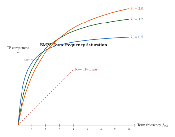
is the term frequency saturation parameter – higher values allow term frequency to have more influence;
is the document length normalisation parameter – means no normalisation, means full normalisation relative to average document length;
is typically computed as: (BM25 IDF)
The BM25 formula has a beautiful structure. The numerator ensures that the contribution grows with term frequency. The denominator introduces saturation: as , the TF component approaches , preventing any single term from dominating the score. The document length normalisation factor ensures that longer documents are not unfairly rewarded simply for containing more terms.
Proposition 2 (BM25 Limiting Behaviours).
The BM25 scoring function exhibits the following limiting behaviours:
: The TF component becomes for all . BM25 reduces to binary term presence weighted by IDF – equivalent to the binary independence model.
: The TF component approaches (linear TF). BM25 reduces to TF-IDF with document length normalisation.
: No document length normalisation. Longer documents are favoured because they naturally contain more term occurrences.
: Full length normalisation. The effective TF is divided by , fully compensating for document length.
Proof.
Part (1): Setting in (BM25), the TF component becomes for . The score reduces to .
Part (2): For large , the denominator is dominated by , so the TF component approaches .
Parts (3) and (4) follow directly from substituting and into the length normalisation factor.
Probabilistic Language Models for Retrieval
An elegant alternative to the vector space approach is to view retrieval through the lens of language modelling. The core idea, introduced by Ponte and Croft (1998), is disarmingly simple: rank documents by the probability that the query was generated by the document's language model.
For each document , we estimate a unigram language model that defines a probability distribution over terms. The probability of generating query from this model is: (Query Likelihood)
The maximum likelihood estimate of is simply the relative frequency: , where is the length of document . But this assigns zero probability to query terms not in the document, making any such document irretrievable. The solution is smoothing:
Jelinek-Mercer smoothing.
(JM Smoothing) where is a smoothing parameter and is the background language model estimated from the entire corpus.
Dirichlet smoothing.
(Dirichlet Smoothing) where is the Dirichlet prior parameter. This has the appealing property that shorter documents are smoothed more heavily (they have less evidence), while longer documents are smoothed less.
Taking the log of the query likelihood and dropping query-independent constants, the ranking function becomes: (LM Ranking) where depends only on the query. The log-ratio is positive when the term is more common in the document than in the corpus – a natural notion of term importance that arises automatically from the probabilistic framework, without the need to hand-design a weighting scheme like TF-IDF.
Theorem 1 (Equivalence of Language Model Retrieval and TF-IDF).
Under Jelinek-Mercer smoothing with , the language model ranking of (LM Ranking) is equivalent to TF-IDF ranking with logarithmic TF and a specific IDF formula. Specifically, for documents of equal length and : (LM Tfidf Equiv) where is a constant independent of .
Proof.
With Jelinek-Mercer smoothing and : for terms present in . The background model is , where is the total count of in the corpus. Then: For equal-length documents, is constant. Writing , where is the average within-document frequency, we get: The first term is logarithmic TF; the second is an IDF-like term; the third is a constant.
The language model approach to retrieval is philosophically significant because it inverts the traditional direction of the retrieval problem. Instead of asking “how similar is this document to the query?” (a matching perspective), it asks “how likely is it that this document generated the query?” (a generative perspective). This inversion – from discriminative matching to generative modelling – is a precursor to the full generative retrieval paradigm that we develop in later sections. When we later study models that generate document identifiers autoregressively, we are taking the language model view of retrieval to its logical conclusion: the entire retrieval process becomes an act of conditional generation.
Remark 5.
The connection between smoothing and the exploration–exploitation trade-off is worth noting. Dirichlet smoothing with small emphasises the document's own statistics (exploitation – trust the document), while large defaults to the corpus statistics (exploration – hedge against sparse data). The optimal trades off between these extremes, and Zhai and Lafferty (2001) showed that works well across many collections – a value that can be interpreted as saying “trust the document after you have seen about 2000 words of evidence.”
Latent Semantic Indexing
The term-document matrix is vast and sparse. A typical corpus with documents and vocabulary yields a matrix with entries, the overwhelming majority of which are zero. Worse, the raw term space suffers from two plagues:
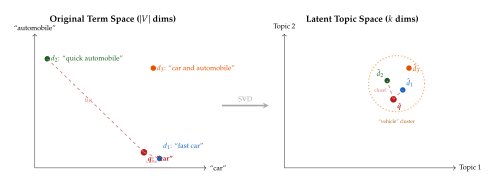
Synonymy: different terms with the same meaning (“car” and “automobile”) have orthogonal representations, so a query for “car” will miss documents about “automobiles.”
Polysemy: the same term with different meanings (“bank”) conflates unrelated concepts into a single dimension.
Latent Semantic Indexing (LSI), introduced by Deerwester et al. [7], addresses both problems by projecting the term-document matrix onto a low-dimensional subspace using the truncated singular value decomposition (SVD).
Let be the TF-IDF-weighted term-document matrix. The rank- truncated SVD is: (SVD) where contains the top left singular vectors (a basis for the “topic” space), is diagonal with the top singular values, and contains the top right singular vectors.
Each document is now represented by the -th row of – a -dimensional vector in the latent topic space. A query is projected into the same space via: (LSI Query)
Retrieval is performed by computing cosine similarity between the projected query and the projected documents.
Theorem 2 (LSI as Optimal Low-Rank Approximation).
The rank- truncated SVD is the optimal rank- approximation to in both the Frobenius norm and the operator (spectral) norm: (Eckart Young) and , where are the singular values of in decreasing order (Eckart–Young–Mirsky theorem).
Remark 6.
LSI was a conceptual breakthrough: it showed that retrieval could benefit from dimensionality reduction, and that the “noise” in the term-document matrix (due to synonymy and polysemy) could be filtered by discarding small singular values. However, LSI has significant practical limitations: the SVD is expensive to compute for large corpora ( for the top components), updating the decomposition when documents are added is non-trivial, and the latent dimensions lack interpretability. These limitations motivated the development of probabilistic topic models.
Latent Dirichlet Allocation
Where LSI finds latent topics via matrix factorisation, Latent Dirichlet Allocation (LDA) discovers them via probabilistic generative modelling [8]. LDA posits that documents are generated by the following process:
For each topic , draw a distribution over words: .
For each document : enumerate
Draw a distribution over topics: .
For each word position in document : enumerate
Draw a topic assignment: .
Draw the word: . enumerate enumerate
Definition 5 (Latent Dirichlet Allocation).
LDA is a generative probabilistic model over a corpus of documents. The joint distribution over observed words and latent variables (topic proportions and topic assignments ) for a single document is: (LDA Joint) The marginal likelihood (evidence) is obtained by integrating over and summing over : (LDA Evidence) This integral is intractable; inference requires variational methods or Markov chain Monte Carlo.
For retrieval, LDA provides a principled way to represent documents as probability distributions over topics. The KL-divergence (or Jensen–Shannon divergence) between topic distributions serves as a similarity measure that captures thematic overlap regardless of lexical overlap: (LDA Retrieval)
Remark 7.
LDA represents a philosophical shift from LSI. Where LSI finds topics by optimising a matrix approximation criterion (minimise reconstruction error), LDA finds topics by fitting a generative model (maximise the probability of the observed data). The generative perspective is crucial: it means that LDA's topics are not just mathematical artefacts but interpretable probability distributions over words. This interpretability – the ability to examine a topic and see that it is “about” medicine, or politics, or cuisine – is one of LDA's enduring contributions.
LDA also reveals a deep connection between generative modelling and retrieval that foreshadows the central theme of this chapter. In LDA, each document is “explained” by a generative story: a mixture of topics, each of which generates words. Retrieval is then the inverse of generation – given the observed words (the query), infer the latent topics, and find documents with similar topic distributions. This pattern – train a generative model, then use its learned representations for retrieval – will recur throughout this chapter at increasing levels of sophistication, from topic models to variational autoencoders to autoregressive language models that generate document identifiers directly.
Proposition 3 (LDA Posterior Intractability).
The posterior distribution in LDA is intractable to compute exactly. Specifically, the normalising constant (evidence) requires summing over possible topic assignments, which is exponential in document length.
Proof.
The evidence is: The sum over has terms (each word can be assigned to any of topics), and the integral over does not factorise because the topic proportions couple all word positions. Both variational inference (which approximates the posterior with a factored distribution) and collapsed Gibbs sampling (which integrates out and samples ) are used in practice.
Evaluation Metrics for Information Retrieval
A retrieval system is only as good as our ability to measure its quality. The field of information retrieval has developed a rich vocabulary of evaluation metrics, each capturing a different aspect of retrieval quality. We present the major metrics here, as they will be used throughout the chapter.
Let be a ranked list of documents produced by a retrieval system for a given query, and let (or for graded relevance) denote the relevance of document .
Definition 6 (Precision and Recall at ).
(Precision AT K) Precision at measures the fraction of retrieved documents (in the top ) that are relevant. Recall at measures the fraction of all relevant documents that appear in the top .
Definition 7 (Average Precision and Mean Average Precision).
The average precision (AP) for a single query is: (AP) AP rewards systems that place relevant documents at the top of the ranked list. The mean average precision (MAP) averages AP over a set of queries: .
Definition 8 (Mean Reciprocal Rank).
The reciprocal rank (RR) is the reciprocal of the rank of the first relevant document: (MRR) The mean reciprocal rank (MRR) averages over queries.
Definition 9 (Discounted Cumulative Gain and nDCG).
For graded relevance judgments , the discounted cumulative gain at position is [3]: (DCG) The logarithmic discount penalises relevant documents that appear deep in the ranked list. The normalised DCG is: (NDCG) where is the DCG of the ideal ranking (documents sorted by decreasing relevance). Thus .
Example 4.
Suppose a query has 5 relevant documents with graded relevance , and a retrieval system returns them in the order with relevance grades for positions 1–5. Then: The ideal ordering gives (the fifth ideal term is ). Hence .
Inverted Indices: The Data Structure of Retrieval
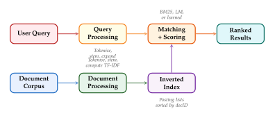
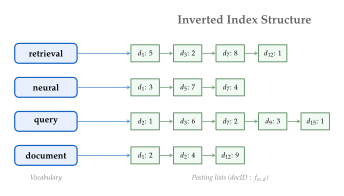
All the scoring functions discussed above – TF-IDF, BM25, query likelihood – share a common computational pattern: they sum contributions from query terms that appear in a document. The naive approach – iterating over all documents for each query – is prohibitively expensive for web-scale corpora. The solution is the inverted index, the fundamental data structure of information retrieval.
Definition 10 (Inverted Index).
An inverted index maps each term in the vocabulary to a posting list – an ordered sequence of pairs for every document containing : (Inverted Index) where the payload typically includes the term frequency and possibly term positions. Posting lists are sorted by docID to enable efficient intersection and union operations.
Algorithm 1 (BM25 Retrieval with Inverted Index).
- Input: Query , inverted index , parameter
- Output: Top- documents ranked by BM25 score
- Initialise score accumulator:
- for each query term
- Compute using (BM25 IDF)
- Retrieve posting list
- for each
- return top- entries from by value
The efficiency of the inverted index comes from a simple observation: most documents do not contain most query terms. For a query with terms, only documents that appear in at least one posting list are scored. If the average posting list length is , the total work is – typically far less than for sparse queries on large corpora.
Comparison of Classical Methods
| Method | Representation | Query Time | Handles Synonymy? | Interpretable? |
| TF-IDF [5] | Sparse, -dim | No | Yes | |
| BM25 [6] | Sparse, -dim | No | Yes | |
| LSI [7] | Dense, -dim | Yes | No | |
| LDA [8] | Dense, -dim | Yes | Yes |
Table 1 summarises the strengths and weaknesses of the classical methods. Sparse methods (TF-IDF, BM25) are fast and interpretable but cannot handle synonym mismatch. Dense methods (LSI, LDA) address synonymy through dimensionality reduction but sacrifice the efficiency of inverted indices – computing similarity in a dense space requires either scanning all documents or building specialised approximate nearest-neighbour indices, which we discuss in later sections.
The resolution of this tension – achieving the semantic power of dense representations with the efficiency of sparse retrieval – is one of the driving forces behind the dense retrieval revolution and the generative retrieval models that are the ultimate subject of this chapter.
It is worth noting that the methods surveyed so far represent only the scoring component of a retrieval system. The broader discipline of learning to rank [43] studies how to learn the scoring function from data, combining multiple signals – BM25 scores, PageRank, click-through data, document freshness, query-document feature vectors – into a single relevance prediction. Learning-to-rank methods (pointwise, pairwise, and listwise) laid the intellectual groundwork for the neural ranking models that would follow, establishing the principle that retrieval scoring should be learned, not hand-designed.
Caution.
BM25 Is Not Dead. Despite the rise of neural retrieval models, BM25 remains a remarkably strong baseline. In many TREC benchmarks and industrial settings, BM25 with careful tuning (, ) is competitive with or superior to naive neural approaches. The lesson: always compare against BM25 before claiming that a neural retrieval model represents an advance. A neural model that cannot beat a well-tuned BM25 is not ready for deployment.
Exercise 9.
Implement TF-IDF from scratch.
Build an inverted index for a small corpus of 10 documents (use any text of your choice).
Implement the TF-IDF scoring function of Definition 3.
Rank the documents for three queries and verify that the results are sensible.
Now implement BM25 (Definition 4) with and . Compare the rankings to TF-IDF. On which queries do they differ, and why?
Exercise 10.
Explore BM25's parameter space.
Plot the BM25 TF component as a function of for with and .
For a fixed query term with in a corpus of , compute the BM25 score for a document where versus . What is the ratio of scores? How does this compare to the ratio under raw TF-IDF?
Prove that BM25's IDF formula ((BM25 IDF)) can assign negative IDF to very common terms (those appearing in more than documents). Is this desirable? Propose a modification that prevents negative IDF.
Exercise 11.
Implement LSI on the “20 Newsgroups” dataset.
Construct the TF-IDF term-document matrix.
Compute the truncated SVD for .
For each value of , evaluate retrieval quality using MAP on a held-out set of queries. Plot MAP versus .
Examine the top 10 terms for the first five latent dimensions. Can you assign interpretable “topic” labels?
Compare retrieval quality to BM25. Under what conditions does LSI outperform BM25?
Exercise 12.
Train an LDA model on a corpus of your choice with topics.
Display the top 10 words for each topic. Assign interpretable labels to at least 10 topics.
Use the inferred topic distributions to retrieve documents for a query. Compare with BM25.
Compute the perplexity of the held-out documents as a function of . Does lower perplexity correlate with better retrieval quality?
Exercise 13.
The choice of evaluation metric can significantly affect system rankings.
Construct a ranked list of 10 documents where MAP ranks system A above system B, but nDCG@10 ranks system B above system A.
Prove that for binary relevance (), nDCG@ reduces to a specific function of precision values at each rank.
Argue that MRR is appropriate when the user wants exactly one answer (e.g., factoid question answering) but inappropriate when multiple relevant documents exist.
We have now laid the three pillars upon which the rest of this chapter stands. The philosophical framework of The Philosophy of Retrieval – What Does It Mean to Remember? established that retrieval is not mere lookup but reconstruction of meaning. The neuroscience of The Neuroscience of Memory and Retrieval showed that the brain implements retrieval through content-addressable memory, pattern completion, and generative reconstruction – mechanisms that neural networks are now learning to emulate. The formal foundations of Formal Foundations of Information Retrieval gave us the mathematical vocabulary – scoring functions, evaluation metrics, indexing structures – that we need to reason precisely about retrieval quality.
In the sections that follow, we will see how deep learning transforms every component of the retrieval pipeline. We begin with the dense retrieval revolution: the replacement of sparse bag-of-words representations with learned dense embeddings that capture semantic meaning. From there, we will progress to the most radical idea in modern retrieval: generative retrieval, where the index, the scoring function, and even the documents themselves are absorbed into the parameters of a single neural network. The journey from TF-IDF to generative retrieval is, in a sense, the journey from Aristotle's associations to Plato's anamnesis – from matching surface patterns to recovering meaning from compressed memory.
Dense Retrieval Revolution
The previous section laid the mathematical foundations of information retrieval in the language of probability, relevance, and term statistics. Those foundations are elegant, but they rest on an assumption so deeply embedded that it is easy to overlook: that documents and queries are best represented by the words they contain. The bag-of-words assumption – that the meaning of a text is captured by the multiset of its tokens – served the field for half a century. It powered TF-IDF, BM25, and the probabilistic models that built the modern web. But it harbours a fatal weakness: it cannot recognise that “automobile” and “car” refer to the same concept, that “heart attack” and “myocardial infarction” describe the same event, that a question about “the capital of France” should match a document that says “Paris is where the French government sits” even though the two texts share almost no words.
This is the vocabulary mismatch problem, and it is not a minor annoyance. Studies have repeatedly shown that users and authors use different words for the same concepts roughly 70–80% of the time [44]. Techniques like query expansion, stemming, and pseudo-relevance feedback provide partial remedies, but they are fundamentally patches on a representational framework that was never designed to capture meaning.
The dense retrieval revolution replaces this framework entirely. Instead of representing documents as sparse vectors over a vocabulary of hundreds of thousands of tokens, dense retrieval maps both queries and documents into a shared continuous vector space of a few hundred dimensions, where semantic similarity is captured by geometric proximity. A query about automobiles and a document about cars end up as nearby points – not because they share tokens, but because a neural network has learned that they share meaning.
The shift from sparse to dense is not merely a change of technique. It is a change of philosophy. Sparse retrieval asks: “Does this document contain the right words?” Dense retrieval asks: “Does this document mean the right thing?” The former is a syntactic question; the latter is a semantic one. And as we shall see, the answer to the semantic question requires us to learn representations – which in turn requires data, computation, and the entire apparatus of modern deep learning.
From Sparse to Dense: The Paradigm Shift
Let us make the contrast precise. In sparse retrieval, a document with vocabulary is represented as a vector where most entries are zero. For BM25, the non-zero entries are the BM25 term weights. The dimensionality is enormous – typically – but the vectors are extremely sparse, with only a few hundred non-zero entries per document. This sparsity enables efficient inverted-index lookups, but it means that two documents can have zero overlap in their representations even when they are semantically identical.
In dense retrieval, we learn an encoder that maps a text (query or document) to a dense vector where is typically 128–1024. Every dimension carries information; there are no structural zeros. Retrieval reduces to finding the documents whose dense vectors are closest to the query vector: (Dense Retrieval) where is typically the inner product or cosine similarity.
Definition 11 (Dense Retrieval Problem).
Given a query encoder , a document encoder , a corpus , and a similarity function , the dense retrieval problem is to return, for each query , the set When we call the architecture a single-encoder (or shared-encoder) model. When they are distinct, we call it a dual-encoder (or bi-encoder) model.
Historical Note.
The idea of mapping documents to dense vectors long predates the neural era. Latent Semantic Indexing (LSI), introduced by Deerwester et al. in 1990, used singular value decomposition to project the term-document matrix into a low-dimensional space. LSI could capture some synonymy – “car” and “automobile” might project to similar vectors – but it operated on the same bag-of-words representations and could not model compositionality or word order. Latent Dirichlet Allocation (LDA) offered a probabilistic alternative in 2003 but suffered from similar limitations. The true revolution came when deep learning provided encoders – first with word2vec and GloVe, then with BERT and its descendants – that could map sequences of tokens to dense vectors that captured syntactic and semantic structure.
DPR: Dense Passage Retrieval
The work that crystallised the dense retrieval paradigm for open-domain question answering was Dense Passage Retrieval (DPR) [45], published by Karpukhin et al. in 2020. DPR demonstrated that a simple dual-encoder architecture, trained with the right contrastive objective, could outperform BM25 on multiple open-domain QA benchmarks – a result that many in the community found surprising, given the decades of engineering that had gone into sparse retrieval systems.
Architecture.
DPR uses two independent BERT encoders: one for
queries () and one for passages ().
Each encoder takes a text as input and produces a -dimensional
vector by extracting the [CLS] token representation from the
final layer:
(DPR Query)
The similarity between a query and a passage is the inner product:
(DPR SIM)
Training objective.
Given a query with a positive passage and a set of negative passages , DPR minimises the negative log-likelihood of the positive passage: (DPR LOSS) This is an instance of the InfoNCE loss [40]. The critical engineering insight in DPR is the use of in-batch negatives: within a mini-batch of query–passage pairs, the positive passage for query serves as a negative for all other queries (), yielding negatives per query at no additional computational cost.
Hard negative mining.
Not all negatives are equally informative. Random negatives are easily distinguished from positives and provide weak gradient signal – their similarity to the query is so low that the softmax in (DPR LOSS) assigns them negligible weight, producing near-zero gradients. DPR addresses this by mining hard negatives – passages that are similar to the query according to BM25 but are not the gold positive. These negatives force the model to learn fine-grained distinctions that go beyond lexical overlap.
Concretely, for each training query, DPR retrieves the top-100 BM25 results and selects passages that do not contain the answer string as hard negatives. The original DPR paper found that using one BM25 hard negative per query, combined with in-batch negatives, yielded the best results. Adding a gold passage from a different query as a “gold negative” provided a further small improvement.
Algorithm 2 (DPR Training with In-Batch Negatives).
- Input: Training set , batch size , learning rate , epochs
- Output: Trained encoders ,
- for to
- for each mini-batch
- for to
- Encode query
- Encode positive passage
- for to
- Encode hard negatives
- In-batch + hard negs
- for to
- Update with gradient using Adam with learning rate
ColBERT: Late Interaction for Token-Level Matching
The dual-encoder architecture of DPR is efficient – query and document encodings are computed independently and can be cached – but it compresses the entire semantics of a passage into a single vector. This is a severe bottleneck. A passage about “the bank of the river” and a passage about “the bank approved the loan” might end up with similar single-vector representations because the word “bank” dominates both, even though the passages are about entirely different topics.
ColBERT (Contextualised Late Interaction over BERT) [46] addresses this by retaining token-level representations and deferring the matching computation to query time. Instead of a single vector per document, ColBERT produces a matrix: (Colbert Query) where and are the token lengths of the query and document, respectively. The similarity is computed via the MaxSim operator: (Maxsim) where is the -th row of and is the -th row of . Each query token finds its best-matching document token, and these maximum similarities are summed.
The MaxSim operator has an intuitive interpretation: it performs a soft word-by-word alignment between query and document. If the query is “When was the Eiffel Tower built?”, the token “Eiffel” will align with the document token “Eiffel” (or “tower” or “Tour”), “built” will align with “constructed” or “completed”, and “when” will align with a date or year token. Each alignment contributes its similarity to the total score, so documents that match on more query tokens receive higher scores. This is far more expressive than a single inner product, which cannot distinguish which aspects of the query are matched.
Remark 8.
The MaxSim operator can be viewed as a soft alignment between query and document tokens. Unlike cross-attention in a cross-encoder, the alignment is computed without any learnable interaction parameters – it is purely geometric. This makes ColBERT a late interaction model: the encoders operate independently, but the final scoring involves token-level interaction.
Proposition 4 (Expressiveness of Late Interaction).
Let denote the family of scoring functions realisable by dual-encoder models (single-vector inner product) and denote the family realisable by late-interaction models with MaxSim. Then .
Proof.
We show (i) inclusion and (ii) strict separation.
Inclusion. Any dual-encoder score can be expressed in the ColBERT framework by setting (single-token representations). Then . Hence .
Strict separation. Consider two documents and with identical mean token embeddings: , but different token-level distributions. A dual-encoder that pools via mean pooling cannot distinguish them: . However, ColBERT's MaxSim can assign different scores by aligning individual query tokens to different document tokens. Concretely, let , with , with , and , . Both documents have the same mean , so the dual-encoder gives score to both. But MaxSim gives for and for . Thus .
Contrastive Learning for Retrieval
The DPR loss in (DPR LOSS) is a specific instance of the InfoNCE objective. Let us state the general form and analyse the role of temperature.
Given an anchor , a positive , and negatives , the InfoNCE loss with temperature is: (Infonce)
The temperature controls the sharpness of the softmax distribution over candidates. Small makes the distribution peaky, assigning nearly all probability to the most similar candidate and creating strong gradients for hard negatives. Large makes the distribution uniform, treating all negatives more equally.
Theorem 3 (Optimal Temperature for Contrastive Retrieval).
Consider the InfoNCE loss in (Infonce) with negatives drawn i.i.d. from a distribution over unit-norm embeddings. Let denote the expected positive similarity and the expected negative similarity, with the standard deviation of negative similarities. In the limit of large , the temperature that minimises the variance of the gradient estimator satisfies (Optimal Temperature)
Proof.
Write the loss as . The gradient with respect to involves the softmax weights where is the partition function. The variance of is dominated by the variance of .
For large , the log-sum-exp concentrates around by a standard Laplace approximation. The effective number of negatives contributing to the gradient is approximately . The gradient variance scales as . Simultaneously, the gradient magnitude scales as . The signal-to-noise ratio of the gradient is therefore Differentiating with respect to and setting the derivative to zero: The correction term arises from finite-sample effects in the Laplace approximation.
Remark 9.
In practice, the temperature is often treated as a learnable parameter (as in CLIP) or tuned on a validation set. The theorem provides guidance: should be proportional to the spread of negative similarities, not set arbitrarily.
SPLADE: Learned Sparse Representations
Dense retrieval captures semantics but sacrifices the efficiency of inverted indices. Sparse retrieval is efficient but misses semantics. SPLADE (SParse Lexical AnD Expansion model) [47] bridges the two worlds by using a neural network to produce sparse representations – vectors in with mostly zero entries – but where the non-zero entries are learned rather than derived from term frequency statistics.
The key idea is to use a BERT-based masked language model head to predict a distribution over the entire vocabulary for each token position, then aggregate across positions: (Splade) where is the contextual representation of the -th token, is the MLM projection matrix, and indexes the vocabulary. The transformation ensures non-negative weights with a saturating growth. SPLADE adds a regularisation term to encourage sparsity: (Splade REG)
Because the resulting representations are sparse and non-negative, they can be stored and searched using standard inverted indices – the same infrastructure that powers BM25. Yet SPLADE performs term expansion: a document about “heart attack” will have non-zero weights for “cardiac”, “myocardial”, and “infarction” even if those words never appear in the text.
Example 5.
Consider the query “What causes high blood pressure?” A BM25 system must match on the exact terms “high”, “blood”, and “pressure”. A SPLADE encoder, having seen many medical texts during training, produces a sparse vector with non-zero weights for “hypertension” (weight 2.8), “blood” (weight 2.1), “pressure” (weight 1.9), “cardiovascular” (weight 1.4), “sodium” (weight 0.9), “arterial” (weight 0.8), and dozens of other related terms. This expansion vector can be looked up in a standard inverted index, bridging the vocabulary gap without the computational cost of dense nearest-neighbour search.
The SPLADE family has evolved through several versions. SPLADE v2 introduced document-side distillation from a cross-encoder, which significantly improved the quality of learned term weights. SPLADE++ further explored the design space of self-distillation and ensemble distillation, achieving results competitive with dense retrieval on the BEIR benchmark while retaining the efficiency of inverted-index retrieval.
Remark 10.
SPLADE occupies a fascinating position in the retrieval landscape: it is technically a sparse method (its representations live in with mostly zero entries), but its representations are semantically dense (the non-zero entries capture meaning far beyond the literal text). This challenges the neat sparse/dense dichotomy and suggests that the fundamental distinction is not about the shape of the vector, but about whether the representation is learned or hand-crafted.
Hybrid Retrieval
In practice, the best retrieval systems combine sparse and dense signals. The intuition is straightforward: sparse retrieval excels at exact lexical matching (entity names, rare terms, identifiers), while dense retrieval excels at semantic matching (paraphrases, synonyms, implicit relevance). The two failure modes are largely complementary.
The simplest hybrid approach is a linear interpolation of scores: (Hybrid Score) where is a mixing weight. Because the two score distributions may have different scales, it is common to normalise each score to before interpolation, for instance via min-max normalisation within the retrieved set: (Hybrid NORM)
A more principled approach is Reciprocal Rank Fusion (RRF), which combines ranked lists rather than scores: (RRF) where is the set of retrieval systems and is a smoothing constant (typically ).
RRF has the advantage of being score-agnostic: it requires only ranked lists, not calibrated scores, making it robust to the different score distributions produced by sparse and dense systems. Empirically, RRF with is remarkably difficult to beat with more sophisticated learned combination methods, a fact that has surprised many researchers.
Multi-stage retrieval.
Production search systems often use a multi-stage pipeline rather than a single fusion step:
First stage (recall). Run BM25 and/or a dual-encoder to retrieve a large candidate set (1000 documents). The goal is high recall, not precision.
Second stage (reranking). Apply a cross-encoder reranker to score each candidate in the context of the query. The cross-encoder sees the concatenation and can model fine-grained query-document interactions.
Third stage (optional). Apply a generative model to rewrite or summarise the top candidates, further improving relevance.
This pipeline exploits the complementary strengths of each approach: fast but coarse first-stage retrieval followed by slow but precise reranking.
Caution.
A common pitfall in hybrid retrieval is score incompatibility: BM25 scores are unbounded and depend on document length, while dense retrieval scores (inner products or cosines) are bounded. Naive interpolation without normalisation can cause one system to dominate the other regardless of . Always normalise scores before combining them, or use rank-based fusion methods like RRF.
Architecture Comparison
The three dominant neural retrieval architectures – dual-encoder, cross-encoder, and late interaction – represent different points on the efficiency-effectiveness trade-off.
Dual-encoder.
The dual-encoder computes query and document representations independently. Document encodings can be precomputed and cached, so online latency scales only with the ANN search cost, not with the number of documents. However, the single-vector bottleneck limits the model's ability to capture fine-grained query-document interactions.
Cross-encoder.
The cross-encoder processes the concatenation through a single transformer, allowing full cross-attention between query and document tokens. This is the most expressive architecture – the model can learn arbitrary interactions between query and document words. But it is also the slowest: each query-document pair requires a separate forward pass, making it impractical as a first-stage retriever for large corpora. Cross-encoders are typically used as rerankers for a small set of candidates retrieved by a dual-encoder or BM25.
Late interaction.
ColBERT's late interaction occupies the middle ground: encodings are independent (enabling precomputation), but scoring involves token-level matching (enabling expressiveness). The storage cost is higher than a dual-encoder ( floats per document instead of ), but ColBERTv2 addresses this with residual compression, reducing storage to approximately 2 bytes per token.
Figure 7 illustrates the key structural differences.
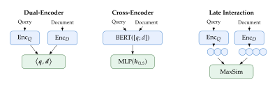
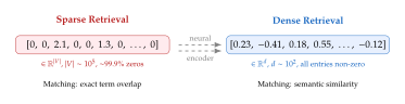
| Method | Top-5 | Top-20 | Top-100 |
| BM25 | 43.8 | 62.9 | 78.3 |
| DPR | 68.3 | 80.1 | 86.1 |
| DPR + BM25 hard negs | 72.1 | 82.6 | 87.3 |
| ColBERT | 73.2 | 83.9 | 88.7 |
| SPLADE v2 | 72.8 | 83.5 | 88.1 |
| Hybrid (BM25 + DPR) | 74.1 | 84.3 | 89.0 |
Exercises
Exercise 14.
Consider a DPR model trained with batch size and hard negative per query. How many total negatives does each query see per training step? If we double the batch size to , by what factor does the number of negatives increase? Discuss why larger batch sizes tend to improve dense retrieval performance.
Exercise 15.
Analyse the computational complexity of ColBERT's MaxSim scoring. Given a query of length and a document of length with embedding dimension , what is the time complexity of computing ? Compare this to the cost of a single inner product in a dual-encoder. How does ColBERTv2's token compression reduce this cost?
Exercise 16.
Implement the InfoNCE loss ((Infonce)) in PyTorch. Train a simple dual-encoder on a synthetic dataset of 10,000 query–passage pairs (embed with random features for simplicity). Sweep the temperature over and plot (a) the final loss, (b) the retrieval accuracy (top-5), and (c) the gradient norm as functions of . Does the optimal align with Theorem 3?
Exercise 17.
A hybrid retrieval system uses the interpolation in (Hybrid Score). Derive the value of that maximises NDCG@10 on a validation set, assuming you have access to relevance labels. Is this a convex optimisation problem? What happens at the boundaries and ?
Approximate Nearest Neighbour Search
Dense retrieval transforms the problem of finding relevant documents into the problem of finding nearby vectors. At training time, we learn to map semantically similar texts to nearby points in . At inference time, we must find, among billions of document vectors, the vectors closest to the query vector. This is the nearest neighbour search problem, and in its exact form it is one of the oldest and most studied problems in computational geometry.
Unfortunately, exact nearest neighbour search in high dimensions is intractable at the scales required by modern retrieval. This is a consequence of the curse of dimensionality: in spaces with more than about 10–20 dimensions, all known exact search algorithms degrade to brute-force linear scan. The intuition is that in high dimensions, distances become increasingly uniform – the ratio between the nearest and farthest neighbour approaches 1 – and geometric partitioning structures (trees, grids, Voronoi cells) become ineffective because query balls intersect exponentially many cells.
For a corpus of vectors in dimensions, a brute-force scan requires floating-point multiplications per query – roughly operations, or about 100 milliseconds on a modern GPU. For an interactive search engine handling thousands of queries per second, this is unacceptable.
More formally, the difficulty is captured by the following observation. Let be points drawn uniformly from . For a query , let be the nearest neighbour and the farthest neighbour. Then for large : (Curse OF DIM) When all distances are approximately equal, the very concept of “nearest neighbour” becomes ill-defined, and no partitioning scheme can prune the search space effectively.
The solution is to accept approximate answers. Approximate nearest neighbour (ANN) methods trade a small amount of accuracy (typically 95–99% of exact recall) for orders-of-magnitude speedups, reducing query latency from seconds to microseconds. The key insight is that for retrieval applications, we do not need the exact nearest neighbour – we need a set of candidates that is good enough to contain the relevant documents, which a subsequent reranking stage can then sort precisely.
Locality-Sensitive Hashing
Locality-sensitive hashing (LSH) was among the first theoretically grounded approaches to ANN search. The key idea is to design hash functions that map similar items to the same hash bucket with high probability and dissimilar items to different buckets.
Definition 12 (Locality-Sensitive Hash Family).
A family is called -sensitive for a distance function if for any :
If , then .
If , then .
The family is useful when and .
For cosine similarity, the standard construction uses random hyperplane hashing. Each hash function is defined by a random vector : (LSH Hyperplane)
Lemma 1 (Collision Probability for Random Hyperplane LSH).
For the random hyperplane hash family, the collision probability is: (LSH Collision) where is the angle between and .
Proof.
The hash function partitions into two half-spaces by the hyperplane . Since is drawn from a spherically symmetric distribution, the hyperplane orientation is uniformly random. Two vectors and receive different hash values if and only if the random hyperplane separates them – i.e., the hyperplane normal falls in the double cone of directions between and .
The fraction of random directions that separate and is exactly , because the set of separating hyperplane normals forms a great circle arc of angular measure out of a total of . Therefore:
A single random hyperplane provides only weak discrimination. If two vectors have angle , the collision probability is – better than chance, but not enough to build a reliable index. To amplify the gap between collision probabilities, we use AND-OR composition: concatenate hash functions to form a band (AND amplification), then use independent bands (OR amplification). Two items collide if they agree on all hashes within at least one band.
The AND step makes the collision probability drop rapidly for dissimilar items (since all hashes must agree), while the OR step ensures that similar items collide in at least one of the bands. The overall collision probability for items at angle is: (LSH Amplified)
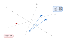
Tree-Based Methods
KD-trees partition space by recursively splitting along coordinate axes. At each node, the dimension with the greatest spread is chosen, and the split is placed at the median value, yielding a balanced binary tree of depth . For query processing, the tree is traversed by following the branch that contains the query, then backtracking to check sibling branches that could contain closer neighbours.
In low dimensions (), KD-trees achieve query times of . In high dimensions, however, the backtracking becomes so frequent that performance degrades to – no better than brute force. Ball trees improve on KD-trees by using hyperspheres rather than axis-aligned splits, which better captures the geometry of clustered data, but they suffer from the same fundamental curse of dimensionality.
The failure of tree-based methods in high dimensions can be quantified precisely. For a KD-tree with points in , the expected number of cells visited during a nearest-neighbour query is: (Kdtree Cells) which for is essentially – brute force.
Remark 11.
Annoy (Approximate Nearest Neighbours Oh Yeah), used by Spotify for music recommendation, uses random-projection trees – a variant of KD-trees where the split direction is chosen randomly rather than along a coordinate axis. By building a forest of many such trees and taking the union of candidates, Annoy achieves reasonable recall in moderate dimensions (). The number of trees controls the accuracy-speed trade-off: more trees yield higher recall at the cost of more memory and slower queries.
Remark 12.
Despite their limitations in high dimensions, tree-based methods remain useful in two scenarios: (1) after dimensionality reduction (e.g., PCA to 32 dimensions), where the effective dimensionality is low enough for trees to work well; and (2) as a component of hybrid indices, where trees provide a coarse first-stage partition that is refined by other methods.
Product Quantization
Product Quantization (PQ) [48] takes a fundamentally different approach: rather than building search structures, it compresses the vectors themselves so that distance computation becomes fast.
The idea is to decompose each -dimensional vector into disjoint subvectors of dimension , quantise each subvector independently using a codebook of centroids, and represent the entire vector by codebook indices. This reduces memory from bits (for float32) to bits – a compression ratio of roughly to depending on (for , : from at to at ).
Definition 13 (Product Quantization).
Let be decomposed into subvectors: where . A product quantizer assigns each subvector to its nearest centroid in a learned codebook : The approximate squared distance between a query and a database vector is: (PQ Distance) where is the centroid index assigned to .
Codebook learning.
The codebooks are learned by running -means independently in each subspace. Specifically, the database vectors are split into subvectors, and -means with clusters is run on each set of subvectors. The total training cost is , which is linear in the database size. The choice of and determines the trade-off between compression ratio and quantisation error. Typical values are – and (so each index fits in one byte), giving PQ codes of 8–64 bytes per vector.
Asymmetric distance computation.
The key efficiency trick is asymmetric distance computation (ADC): we do not quantise the query. Instead, we precompute a lookup table of distances for all subspaces and all centroids – a table of size . Then the distance to any database vector requires only table lookups and additions, regardless of . The lookup table computation costs , which is amortised over all database vectors. The total query cost is therefore , which for , , is roughly – dominated by the term, which is of the brute-force cost.
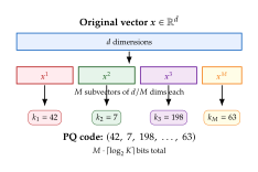
HNSW: Hierarchical Navigable Small World Graphs
Hierarchical Navigable Small World (HNSW) [49] is currently the most widely used ANN index, powering systems from Faiss to Pinecone to Weaviate. It combines two ideas: the navigable small world property of proximity graphs and a hierarchical structure inspired by skip lists.
Navigable small world graphs.
A navigable small world (NSW) graph connects each vector to a set of neighbours. Crucially, each node maintains both short-range links (to nearby vectors) and long-range links (to distant vectors). This combination enables greedy search – always moving to the neighbour closest to the query – to find near-optimal results in polylogarithmic time, analogous to the “six degrees of separation” phenomenon in social networks. The theoretical foundation is Kleinberg's result on navigable networks: if long-range links are distributed according to an inverse-power-law of distance, greedy routing finds near-optimal paths in steps.
Hierarchical structure.
HNSW organises the NSW graph into layers, numbered (bottom, containing all vectors) through (top, containing very few vectors). Each vector is assigned a maximum layer where is a normalisation constant. This gives an exponentially decaying probability of appearing in higher layers – exactly like a skip list.
Search proceeds top-down: starting from the entry point at the top layer, greedy search finds the closest node in that layer, then descends to the next layer using that node as the starting point, and repeats. The upper layers provide long-range navigation, while the bottom layer provides fine-grained local search.
Algorithm 3 (HNSW Search).
- Input: Query , entry point at layer , number of neighbours , candidate list size
- Output: Approximate -nearest neighbours
- Current best set
- for downto Greedy search in upper layers
- Keep only 1 candidate
- Beam search in bottom layer
- return top- from by distance to
- function SearchLayer
- Candidate set
- Visited set
- while
- nearest element in to
- farthest element in from
- if
- break No improvement possible
- Remove from
- for each neighbour of at layer
- if
- farthest element in from
- if or
- if
- Remove farthest element from
- return
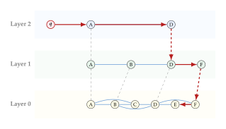
Construction.
Index construction inserts vectors one at a time. For each new vector , a random maximum layer is drawn from the geometric distribution. The algorithm then searches the current graph (top-down, as in the query algorithm) to find the closest neighbours of at each layer , and creates bidirectional edges to those neighbours. If a neighbour's edge count exceeds a maximum , the weakest edges are pruned using a heuristic that favours diverse connections – neighbours are kept only if they are closer to than to any already-selected neighbour. This diversity-preserving heuristic is crucial: without it, the graph degenerates into local clusters with poor long-range connectivity.
The construction cost per vector is , where is the candidate list size used during insertion (typically much larger than the search ). Total index construction is therefore .
Complexity analysis.
The number of layers is , and greedy search at each layer visits nodes (under mild distributional assumptions). The total search complexity is therefore distance computations, each costing . The parameter (candidate list size at the bottom layer) provides a tunable knob: larger improves recall at the cost of more distance computations, scaling the bottom-layer cost to .
Memory overhead.
Each vector stores edges per layer, and the expected number of layers per vector is . The total memory overhead for edges is approximately bytes (storing neighbour indices as 32-bit integers). For and , this is roughly 160 GB for edges alone – a significant cost that must be added to the storage of the vectors themselves.
Caution.
HNSW's main weakness is memory consumption. Unlike IVF-PQ, which compresses vectors to a few bytes each, HNSW requires storing the full float32 vectors (for distance computation during search) plus the graph edges. For billion-scale collections, this can require terabytes of RAM. Hybrid approaches – using IVF for coarse partitioning and HNSW within each partition – can reduce this cost, as can combining HNSW with quantised vectors (at the expense of some recall).
IVF: Inverted File Index
The Inverted File Index (IVF) partitions the vector space into Voronoi cells using -means clustering. Each database vector is assigned to its nearest centroid. At query time, only the vectors in the closest cells are searched:
Offline. Run -means on the database vectors to obtain centroids . Assign each vector to its nearest centroid and store in the corresponding inverted list.
Online. Compute distances from the query to all centroids. Select the nearest centroids. Exhaustively search the vectors in those inverted lists.
The expected number of distance computations per query is , which for typical values (, ) is roughly – a dramatic reduction from .
Residual encoding.
A refinement of IVF stores not the original vectors but the residuals – the difference between each vector and its assigned centroid: where is the cell assignment of . At query time, the query residual is computed for each probed cell , and distances are measured in residual space. Because residuals have smaller variance than the original vectors (the centroid has “explained” the coarse location), they can be quantised more accurately with the same number of bits.
IVF-PQ.
The IVF index can be combined with Product Quantization: the inverted lists store PQ-encoded residual vectors instead of full float32 vectors. This combination – IVF-PQ – is the workhorse of billion-scale retrieval systems, offering both fast search (via cell pruning) and low memory (via vector compression). Faiss's implementation of IVF-PQ can index one billion 768-dimensional vectors in approximately 64 GB of RAM (with and ), compared to roughly 3 TB for storing the raw float32 vectors.
Multi-probe IVF.
The parameter creates a direct trade-off between recall and latency. With , only the nearest cell is searched – fast but inaccurate if the query lies near a cell boundary. With , all cells are searched – exact but slow. Empirically, provides a good balance, achieving 90–95% recall at a fraction of the brute-force cost.
ScaNN: Anisotropic Quantization for MIPS
Most ANN methods are designed for Euclidean distance or cosine similarity, but retrieval models often optimise the inner product , which does not correspond to a metric (it can be negative and does not satisfy the triangle inequality). ScaNN [50] introduces anisotropic vector quantization, which recognises that when optimising inner products, errors in the direction of the query matter more than errors in orthogonal directions.
Standard PQ minimises the isotropic reconstruction error . ScaNN instead minimises a weighted error that penalises the component parallel to the query direction more heavily: (Scann LOSS) This is not equivalent to minimising unless the query distribution is isotropic.
In more detail, ScaNN decomposes the quantisation error into a component parallel to and a component perpendicular to : (Scann Decomp) The parallel error directly affects the inner product estimate, while the perpendicular error has zero expected effect (assuming isotropic query distribution). ScaNN assigns a weight to the parallel component during codebook optimisation, focusing the quantiser's limited capacity on the dimension that matters most for MIPS.
Remark 13.
ScaNN also incorporates a score-aware quantisation scheme that allocates more codebook capacity to database vectors with large norms (which are more likely to be retrieved for many queries). This non-uniform allocation further improves the recall-latency trade-off compared to standard PQ.
Recall-Latency Trade-Off
Proposition 5 (Recall-Latency Trade-Off).
Let denote the recall@ of an ANN method as a function of the average query latency . Under mild assumptions (the data distribution has bounded density and the search structure has logarithmic diameter), the recall satisfies: (Recall Latency) where depends on the data distribution and depends on the ANN method and index parameters.
Proof sketch.
The recall deficit corresponds to the probability that the true nearest neighbour lies outside the searched region. For graph-based methods like HNSW, increasing the search budget (candidate list size ) expands the searched region exponentially – each additional step explores a constant factor more of the graph. Since the probability of missing a neighbour decays exponentially with the volume of the searched region, and the latency scales linearly with the number of distance computations, we obtain the exponential decay bound. The constants and depend on the graph connectivity, the intrinsic dimensionality of the data, and the number of neighbours .
| Method | Build | Query | Memory | Recall@10 | Updatable |
| LSH | High | 85–92% | Yes | ||
| PQ () | 64 B | 70–85% | No | ||
| HNSW | 3 KB + links | 95–99% | Yes | ||
| IVF-PQ | 64 B | 80–92% | Partial | ||
| ScaNN | 64 B | 85–95% | No |
Key Idea.
At billion scale, no single ANN method dominates. Production systems typically combine multiple techniques: IVF for coarse partitioning, PQ for compression, and graph-based reranking for precision. The choice depends on the application's requirements for latency, memory, recall, and updateability. Facebook's Faiss library, Google's ScaNN, and the open-source HNSWlib each implement different combinations of these building blocks.
Exercises
Exercise 18.
An LSH index uses hash functions per band and bands. Using (LSH Amplified), compute the collision probability for two vectors at angles , , and . Plot as a function of for . How would you adjust and to make the transition from high to low probability sharper?
Exercise 19.
A product quantizer with subspaces and centroids encodes a 768-dimensional vector. (a) How many bytes does the PQ code require? (b) What is the maximum quantisation error per subvector, expressed in terms of the codebook and the data distribution? (c) Derive the expected total quantisation error as a sum over subspace distortions.
Exercise 20.
Implement HNSW graph construction for a dataset of random vectors in . Use (max connections per layer), (max connections at layer 0), and . Measure the search recall@10 as a function of for . Does the recall-latency curve follow the exponential form of Proposition 5?
Exercise 21.
Prove that for uniformly distributed data in , the optimal number of Voronoi cells in an IVF index is , where is the database size. Hint: balance the cost of centroid comparison () against the cost of exhaustive search within probed cells ().
Embedding Models and Training
The dense retrieval methods of Dense Retrieval Revolution depend entirely on the quality of the underlying embeddings. A dual-encoder is only as good as the vectors it produces – if semantically similar texts are not mapped to nearby points, no amount of ANN engineering will salvage retrieval quality. This section traces the evolution of embedding models from early Siamese networks to modern universal embedding systems, and examines the training techniques that make them effective.
Sentence-BERT: The Foundation
Before Sentence-BERT [51], using BERT for sentence similarity required passing every pair through a cross-encoder – forward passes for sentences. Sentence-BERT (SBERT) introduced the idea of fine-tuning BERT in a Siamese architecture to produce fixed-size sentence embeddings that could be compared with cosine similarity.
Architecture.
SBERT passes each sentence independently through a shared BERT encoder, applies a pooling operation (typically mean pooling over token embeddings) to obtain a sentence vector, and optimises a contrastive or regression objective: (Sbert Embedding) where is the contextual embedding of the -th token and is the sequence length. For natural language inference (NLI) training, SBERT uses a softmax classifier over the concatenation , while for semantic textual similarity (STS) it uses cosine similarity with a regression objective.
Remark 14.
The choice of pooling matters more than one might expect. While
BERT's original design used the [CLS] token as a sentence
representation, Reimers and Gurevych showed that mean pooling
consistently outperforms [CLS] pooling for sentence
similarity tasks. The intuition is that mean pooling aggregates
information from all tokens, while the [CLS] token in
base BERT is optimised for next-sentence prediction, not for
general-purpose similarity.
Training objectives.
SBERT explores several training configurations depending on the available supervision:
Classification objective (NLI). Given sentence pairs labelled as entailment, contradiction, or neutral, the model concatenates and passes it through a softmax classifier. This trains the embeddings to be informative about semantic relationships.
Regression objective (STS). Given sentence pairs with continuous similarity scores , the model minimises the mean squared error between and .
Contrastive objective (retrieval). Given query–positive pairs, the model uses the multiple negatives ranking loss with in-batch negatives.
The key finding of the original SBERT paper was that NLI pre-training followed by STS fine-tuning produced the best general-purpose embeddings – a recipe that influenced all subsequent work.
Example 6.
To illustrate the impact of SBERT, consider the task of finding the most similar sentence among 10,000 candidates for a given query. With a cross-encoder, this requires 10,000 BERT forward passes (one per pair), taking roughly 65 seconds on a single GPU. With SBERT, the candidate embeddings are precomputed once, and the query is compared to all candidates via matrix multiplication in approximately 5 milliseconds – a speedup of over 10,000.
Instruction-Conditioned Embeddings
A limitation of early embedding models is that they produce a single embedding per text, regardless of the downstream task. But the “meaning” of a sentence depends on what you intend to do with it. For clustering, you want to capture the topic. For retrieval, you want to capture the information need. For classification, you want to capture the label-relevant features.
Instructor [52] and E5 [53] address this by prepending a task instruction to the input text: (Instructor) where denotes string concatenation. Different instructions steer the encoder towards different aspects of the text's meaning, enabling a single model to serve multiple tasks.
E5 (EmbEddings from bidirEctional Encoder rEpresentations) further refined this approach by training on massive curated datasets of text pairs with task-specific prefixes (“query:” and “passage:”), achieving strong zero-shot performance across diverse benchmarks.
The importance of instructions can be understood geometrically. Without instructions, the model must map a sentence to a single point in that is simultaneously close to all “similar” sentences – but similarity is task-dependent. For clustering, “The stock market rose today” should be near other finance sentences; for sentiment analysis, it should be near other positive sentences. Instruction conditioning effectively gives the model access to a different projection for each task, expanding the effective capacity of the embedding space without increasing dimensionality.
Example 7.
Consider the sentence “Python is great for data science.” With the instruction “Represent this sentence for topic classification”, the embedding emphasises the programming and data science aspects. With “Represent this sentence for sentiment analysis”, the embedding emphasises the positive sentiment (“great”). With “Represent this sentence for retrieving tutorials”, the embedding emphasises the instructional aspects. A single model produces three different – and contextually appropriate – embeddings.
Modern Open Embedding Models
The period from 2023 onward saw rapid progress in open-source embedding models, driven by improved training data, multi-stage training pipelines, and architectural innovations.
GTE (General Text Embeddings).
Developed by Alibaba, GTE uses a multi-stage training pipeline: (1) unsupervised pre-training with contrastive learning on web-scale text pairs, (2) supervised fine-tuning on curated retrieval datasets, and (3) task-specific adaptation. GTE models range from 100M to 1.5B parameters and achieve state-of-the-art results on the MTEB benchmark.
BGE (BAAI General Embedding).
Developed by the Beijing Academy of Artificial Intelligence, BGE similarly employs multi-stage training with an emphasis on hard-negative mining across stages. A notable innovation is RetroMAE pre-training, which uses masked autoencoding with an asymmetric architecture to learn better representations before contrastive fine-tuning.
Training at scale.
The key insight behind both GTE and BGE is that data quality and quantity matter more than architectural innovation for embeddings. Both groups invested heavily in curating large-scale training datasets:
Web-mined pairs. Title-body pairs from web pages, question-answer pairs from forums, and anchor-text-to-page mappings provide hundreds of millions of weakly supervised pairs.
Synthetic data. Large language models generate query-passage pairs for domains where natural pairs are scarce (e.g., scientific and legal texts).
Cross-lingual alignment. Parallel translations and bilingual dictionaries enable multilingual embedding models that map semantically equivalent texts in different languages to nearby vectors.
Remark 15.
The MTEB (Massive Text Embedding Benchmark) has become the standard evaluation suite for embedding models. It spans seven task categories – classification, clustering, pair classification, reranking, retrieval, STS, and summarisation – across 56 datasets. A model's MTEB average score provides a single-number summary of embedding quality, though the score should be interpreted with caution: strong performance on retrieval tasks does not guarantee strong performance on classification, and vice versa.
Matryoshka Representation Learning
A practical challenge with embedding models is that different applications have different computational budgets. A mobile application might afford only 64-dimensional embeddings, while a server-side system can handle 1024 dimensions. Traditionally, this required training and maintaining separate models for each dimensionality.
Matryoshka Representation Learning (MRL) [54] trains a single model whose embeddings are useful at any prefix dimensionality. Named after the Russian nesting dolls, MRL ensures that the first dimensions of a -dimensional embedding form a good -dimensional embedding.
The training loss is a weighted sum over multiple truncation levels: (Matryoshka LOSS) where is a set of target dimensionalities, denotes the first dimensions of the embedding, are weights (often uniform), and is the standard contrastive loss applied at each scale.
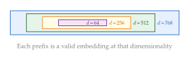
The key property that makes MRL work is that the information content of the embedding is front-loaded: the first few dimensions capture the coarsest, most important distinctions (broad topic, language, domain), while later dimensions encode progressively finer details (specific entities, subtle sentiment, stylistic nuances). Without the Matryoshka loss, a standard contrastive training procedure distributes information more uniformly across dimensions, so truncation causes a sharp quality drop.
Example 8.
Consider a 768-dimensional MRL-trained embedding of the sentence “The cat sat on the mat.” The first 8 dimensions might encode that this is English prose about animals. The first 64 dimensions additionally encode that it involves a domestic cat, a static scene, and a physical location. The first 256 dimensions further encode the syntactic structure, the definiteness of the noun phrases, and the simplicity of the sentence. The full 768 dimensions capture everything, including subtle stylistic markers that distinguish this sentence from “A cat was sitting upon a mat.”
Remark 16.
MRL has been adopted by several production embedding models,
including OpenAI's text-embedding-3-* family and Cohere's
Embed v3. The practical benefit is substantial: users can trade off
embedding quality for storage and compute without retraining. At
256 dimensions, MRL-trained models retain 95–98% of the full
768-dimensional performance on most benchmarks. A common deployment
pattern is to use 256-dimensional embeddings for first-stage ANN
retrieval (reducing memory by 3) and full 768-dimensional
embeddings for reranking the top candidates.
Long-Context Embeddings
Standard BERT-based embeddings are limited to 512 tokens – roughly a paragraph. Many retrieval applications require embedding entire documents, legal filings, or codebases that span thousands of tokens.
Nomic Embed.
Nomic Embed extends the context window to 8,192 tokens using ALiBi (Attention with Linear Biases) positional encoding, which replaces learned absolute position embeddings with a linear bias term that decays with token distance. This allows the model to generalise to sequence lengths not seen during training.
jina-embeddings.
The jina-embeddings family uses a modified BERT architecture with RoPE (Rotary Position Embeddings) to support context lengths up to 8,192 tokens. jina-embeddings-v3 further introduces Late Chunking: rather than embedding each chunk independently, it processes the full document through the transformer and then extracts chunk embeddings from the contextual representations, preserving cross-chunk coherence.
The chunking dilemma.
Long-context embeddings address a fundamental tension in document retrieval. Short chunks (128–256 tokens) are precise – each chunk covers a single topic – but they lose context. A chunk saying “He won the award in 1995” is useless without knowing who “he” is. Long chunks (2048+ tokens) preserve context but dilute the embedding: a 2000-token passage about multiple topics produces a vector that is an imprecise average of several distinct meanings.
The ideal solution would embed each passage with full awareness of its surrounding context – which is exactly what Late Chunking achieves, and what long-context models make feasible by processing entire documents through the transformer before extracting per-chunk embeddings from the contextualised representations.
Gemini Embedding: Universal Multimodal Embeddings
The trajectory from single-task text embeddings to multi-task instruction-conditioned embeddings finds its logical continuation in universal multimodal embedding models that map text, images, code, and other modalities into a shared vector space.
Definition 14 (Universal Embedding Model).
A universal embedding model is a function where is the union of modality spaces (e.g., text, images, audio, code), such that for any pair of inputs (possibly cross-modal), the similarity is a meaningful measure of semantic relatedness.
Gemini Embedding is Google's entry in this space. Built on the Gemini multimodal architecture, it produces embeddings that can be used for text retrieval, code search, image-text matching, and cross-lingual transfer within a single model. The architecture leverages Gemini's native multimodal understanding to produce embeddings without modality-specific encoder heads. Key design choices include:
Instruction-conditioned. Like Instructor and E5, Gemini Embedding accepts task instructions, but extends this to multimodal queries (e.g., “Find images similar to this description”).
Shared latent space. All modalities are projected into the same -dimensional space, enabling zero-shot cross-modal retrieval.
Matryoshka-compatible. The model supports flexible dimensionality via MRL-style training.
The move towards universal multimodal embeddings raises fundamental questions about the geometry of the shared space. When text, images, and code are all mapped to , the model must learn to organise semantically related items of different modalities nearby while keeping unrelated items of the same modality apart. This creates a tension: the model must simultaneously optimise intra-modal discrimination and cross-modal alignment. Early multimodal embedding models like CLIP resolved this by training exclusively on cross-modal pairs (image-text), but this left intra-modal performance suboptimal. Modern models like Gemini Embedding train on a mixture of within-modal and cross-modal contrastive objectives, with careful balancing of the loss weights.
Remark 17.
The dimensionality of Gemini Embedding (3072) is notably higher than most text-only models (768–1024). This is not accidental: the shared space must accommodate multiple modalities, each with its own internal structure. Higher dimensionality provides more capacity for the model to carve out modality-specific subspaces while maintaining a shared semantic core. The cost is increased storage and search latency, partially mitigated by MRL-style dimensionality reduction.
The Embedding Training Pipeline
State-of-the-art embedding models are not trained in a single pass. They follow a multi-stage pipeline that progressively refines representations:
Stage 1: Pre-training.
The base language model (typically a BERT variant or decoder model) is pre-trained on a large unlabelled corpus with masked language modelling (MLM) or causal language modelling (CLM). This stage provides general linguistic knowledge but does not produce good sentence-level representations.
Stage 2: Contrastive pre-training.
The model is further pre-trained with a contrastive objective on weakly supervised text pairs – typically title-body pairs, question-answer pairs, and parallel translations harvested from the web. This stage – sometimes called unsupervised contrastive learning or weakly-supervised pre-training – teaches the model to recognise semantic similarity at the sentence level. The scale of data at this stage is massive: GTE uses over 800 million text pairs, and E5 uses a curated dataset of over 300 million pairs spanning 93 languages.
Stage 3: Supervised fine-tuning.
The model is fine-tuned on curated, high-quality labelled datasets with hard negatives. This is where most of the retrieval-specific learning happens. The loss is typically InfoNCE with in-batch negatives and mined hard negatives.
Stage 4: Distillation (optional).
A smaller student model is trained to mimic the similarity judgements of a larger teacher model (often a cross-encoder). The distillation loss is typically a KL divergence between the student's and teacher's softmax distributions over candidates: (Embedding Distill) where and are the vectors of scores assigned by teacher and student to a set of candidates, is the softmax function, and is a distillation temperature. This allows production deployment of efficient models (100M–300M parameters) that approach the quality of expensive cross-encoders (which may have billions of parameters but cannot precompute embeddings).
The distillation pipeline typically works as follows: (1) retrieve the top 100 candidates for each training query using a first-stage retriever; (2) score all 100 candidates with the cross-encoder teacher; (3) train the student embedding model to reproduce the teacher's ranking, using the KL divergence loss in (Embedding Distill). The student never sees the teacher's internal representations – only its output scores. This score distillation approach is simpler and more effective than feature-level distillation for embedding tasks, because what matters for retrieval is the relative ordering of candidates, not the internal features used to produce that ordering.

Training Objectives: Contrastive vs. Generative
The dominant training paradigm for embeddings is contrastive learning, but an alternative generative approach has gained traction.
Contrastive objectives.
The standard approach uses InfoNCE ((Infonce)) with temperature scaling. Variants include:
Triplet loss: where is a margin.
Multiple negatives ranking loss: The in-batch softmax cross-entropy, which is equivalent to InfoNCE with .
Cosine similarity loss: Direct regression of cosine similarity to human-annotated similarity scores.
Generative objectives.
Recent work has shown that decoder-based language models can produce strong embeddings by encoding the text as a prompt and extracting embeddings from the last token representation. The key insight is that the last token in a causal model has attended to all preceding tokens, making its representation a natural summary of the input.
Several approaches have emerged for extracting embeddings from LLMs:
LLM2Vec: Converts any decoder LLM into a bidirectional encoder by enabling bidirectional attention (removing the causal mask) and training with a contrastive objective. This preserves the LLM's world knowledge while enabling symmetric encoding.
E5-Mistral: Fine-tunes Mistral-7B with instruction-following and contrastive learning, using the last token embedding. Achieves state-of-the-art MTEB scores while operating with the original causal attention.
Gecko: Google's approach of distilling knowledge from a large LLM into a compact embedding model by using the LLM to generate diverse query-passage training pairs with fine-grained relevance labels.
The advantage of LLM-based embeddings is leveraging the massive scale and world knowledge of pre-trained models (7B+ parameters) for embedding tasks. The disadvantage is computational: encoding a single text with a 7B-parameter model is roughly 20 slower than with a 335M-parameter BERT model, which can be prohibitive for applications that require real-time indexing of new documents.
Hard Negative Mining Strategies
The quality of negative examples is arguably the most important factor in embedding training. We describe three strategies in order of increasing effectiveness.
BM25 negatives.
The simplest hard negatives are passages retrieved by BM25 for the query that are not in the gold positive set. These negatives share lexical overlap with the query, forcing the model to learn that surface similarity does not imply relevance. This is the strategy used by DPR.
Cross-encoder negatives.
A stronger approach uses a cross-encoder reranker to score a large candidate set retrieved by a first-stage model. Passages that the cross-encoder scores highly but that are not in the gold set become hard negatives. These negatives require the embedding model to match the fine-grained discriminative ability of the cross-encoder.
Self-negatives.
In iterative training, the embedding model itself is used to retrieve negatives. After each training epoch, the model re-indexes the corpus, retrieves the hardest non-positive passages for each query, and uses them as negatives for the next epoch. This creates an adversarial curriculum that progressively challenges the model. The process is analogous to self-play in reinforcement learning: the model generates its own training signal by identifying its current failure modes.
The practical challenge with self-negatives is computational: re-indexing a large corpus after each epoch requires encoding all documents with the updated model. A common approximation is to re-index every epochs or to use an exponential moving average of the model weights for indexing, which reduces but does not eliminate the staleness of the negative set. The ANCE (Approximate Nearest Neighbour Negative Contrastive Learning) method formalised this approach, showing significant gains over static negative mining on multiple benchmarks.
Proposition 6 (Hard Negatives Improve Gradient Signal).
Consider the InfoNCE loss with temperature , an anchor , a positive , and negatives. Let denote the logit for the -th negative. The gradient with respect to the query encoder satisfies: (Hardneg Gradient) where are the softmax weights over negatives. Hard negatives (large ) receive large softmax weights , thereby contributing more to the gradient norm.
Proof.
The InfoNCE loss can be written as: Differentiating with respect to : Denoting the softmax probabilities as and where is the partition function: The negative contribution to the gradient norm is: by Cauchy–Schwarz. However, the lower bound follows from Jensen's inequality applied to the convex function : For the component-wise bound, note that when the negatives are not all identical. The weights are monotonically increasing in : harder negatives (those with higher similarity to the query) receive exponentially larger weights, concentrating the gradient on the most informative negatives. Dividing by completes the bound.
Insight.
The embedding quality ladder describes the empirical observation that embedding quality depends on training data quality in a predictable hierarchy:
Random negatives: The model learns to distinguish obviously irrelevant passages (easy).
BM25 negatives: The model learns that lexical overlap semantic relevance (moderate).
Cross-encoder negatives: The model approaches cross-encoder-level discrimination (hard).
Iterative self-negatives: The model continuously improves by finding its own failure modes (hardest).
Each rung of the ladder yields diminishing but consistent improvements in retrieval quality. The best models climb all four rungs during training.
Embedding Model Comparison
| Model | Params | Dims | Context | MTEB Avg | Key Feature |
| SBERT (2019) | 110M | 768 | 512 | 56.3 | Siamese BERT |
| E5-base (2022) | 110M | 768 | 512 | 59.9 | Task prefixes |
| BGE-large (2023) | 335M | 1024 | 512 | 64.2 | RetroMAE pre-training |
| GTE-large (2023) | 335M | 1024 | 512 | 65.4 | Multi-stage pipeline |
| Nomic-embed (2024) | 137M | 768 | 8192 | 62.4 | Long context (ALiBi) |
| jina-v3 (2024) | 570M | 1024 | 8192 | 66.1 | Late Chunking |
| E5-mistral-7B (2024) | 7.1B | 4096 | 32768 | 66.6 | LLM-based |
| Gemini Embed (2025) | - | 3072 | 8192 | 67.5 | Multimodal universal |
The trend is clear: models have grown in parameter count, embedding dimensionality, context length, and benchmark performance. But perhaps the most important trend is the convergence towards universal models that handle multiple tasks, languages, and modalities within a single architecture.
Several observations emerge from this comparison. First, the jump from SBERT to E5 (3.6 points) came primarily from better training data, not architectural changes – both use similar BERT-based architectures. Second, the LLM-based models (E5-mistral-7B) achieve the highest scores but at 20 the computational cost, raising the question of whether the quality gain justifies the expense for latency-sensitive applications. Third, long-context models (Nomic, jina) sacrifice a few MTEB points for dramatically expanded context windows – a trade-off that is worthwhile for document-level retrieval but unnecessary for short-query tasks.
Exercises
Exercise 22.
Implement three pooling strategies for a BERT encoder: (a)
[CLS] token, (b) mean pooling, and (c) max pooling. Using
a pre-trained BERT-base model (without fine-tuning), compute
sentence embeddings for the STS Benchmark dataset and evaluate
Spearman correlation with human similarity judgements. Which pooling
strategy performs best, and why?
Exercise 23.
Train a small embedding model (e.g., DistilBERT) with and without the Matryoshka loss ((Matryoshka LOSS)) on a retrieval dataset of your choice. For both models, evaluate retrieval accuracy (recall@10) at dimensions by truncating the embedding. At what dimensionality does the Matryoshka-trained model start to significantly outperform the standard model?
Exercise 24.
Design an experiment to validate the embedding quality ladder described in the Insight box. Train four versions of the same dual-encoder model on the same dataset, varying only the negative mining strategy: (i) random, (ii) BM25, (iii) cross-encoder, and (iv) self-negatives with 3 re-indexing iterations. Report recall@10 and NDCG@10 on a held-out test set. Does the ranking of strategies match the predicted hierarchy?
Exercise 25.
Consider a universal embedding model (Definition 14) that maps text and images to . (a) Explain why training with only text–text and image–image pairs might produce a model where text and image embeddings occupy disjoint regions of the space. (b) Propose a training objective that explicitly encourages cross-modal alignment. (c) Discuss the tension between modality-specific discriminative power and cross-modal alignment – can you have both?
Classical Vision Retrieval
Imagine you are sitting in a small café in Lisbon. On the wall hangs a painting: a turbulent sky rendered in thick impasto strokes, deep blues swirling above a sleeping village. You do not know the artist or the title, but you want to find it online. You could describe it in words, but language is an impoverished medium for capturing visual texture, colour palette, and compositional geometry. What you really want is to take a photograph and ask a system: find me this painting. This is the problem of image retrieval: given a query image, find the most visually similar images in a large database.
The story of how computer vision solved this problem is one of the most elegant intellectual arcs in the field. It begins with a deceptively simple insight: images, like documents, can be represented as collections of discrete visual features. This insight connects the rich mathematical machinery of text retrieval, which we developed in the preceding sections, to the entirely different modality of visual perception. The bridge between these two worlds was built by local feature descriptors, most notably the Scale-Invariant Feature Transform.
SIFT: Scale-Invariant Feature Transform
The fundamental challenge of image matching is that the same object looks different under different viewing conditions. A photograph of a cathedral taken from ten metres away at noon and another taken from thirty metres away at sunset depict the same structure, yet nearly every pixel value differs. The genius of David Lowe's Scale-Invariant Feature Transform (SIFT) [55] is to extract local image features that remain stable under changes in scale, rotation, and illumination, precisely the transformations that make naïve pixel-level comparison fail.
Definition 15 (Local Feature Descriptor).
A local feature descriptor is a function that maps an image and a keypoint location (position, scale, orientation) to a -dimensional vector such that is approximately invariant to a group of geometric and photometric transformations : (Invariance) where denotes the transformed image and the correspondingly transformed keypoint.
The SIFT algorithm proceeds in four stages, each building carefully on the last. We describe each in turn.
Stage 1: Scale-space extrema detection.
The first stage identifies candidate keypoint locations that are stable across scales. SIFT constructs a scale space by convolving the image with Gaussian kernels of increasing width: (Scale Space) Keypoint candidates are found at extrema of the Difference of Gaussians (DoG): (DOG) where is a constant multiplicative factor separating adjacent scales. A point is a candidate keypoint if is a local extremum in both spatial coordinates and scale, compared to its neighbourhood of 26 adjacent samples.
Stage 2: Keypoint localisation.
Each candidate is refined by fitting a three-dimensional quadratic to the DoG function via a Taylor expansion: (Keypoint Refine) where . The extremum is located at , and candidates with low contrast or high edge response (ratio of principal curvatures above a threshold) are discarded.
Stage 3: Orientation assignment.
Each surviving keypoint is assigned one or more dominant orientations based on a histogram of gradient orientations in a neighbourhood weighted by the keypoint's scale. Let and be the gradient magnitude and orientation. A 36-bin orientation histogram is computed, and any peak within 80% of the maximum defines a keypoint orientation. This step ensures rotational invariance: all subsequent computations are performed relative to the assigned orientation.
Stage 4: Descriptor construction.
The descriptor is computed in a patch around the keypoint, rotated to align with the assigned orientation. This patch is divided into a grid of sub-regions, and within each sub-region an 8-bin orientation histogram is computed, weighted by gradient magnitude and a Gaussian centred on the keypoint. The result is a -dimensional vector , which is normalised to unit length to achieve illumination invariance: (SIFT Descriptor)
Proposition 7 (SIFT Invariance Properties).
The SIFT descriptor achieves the following invariance properties:
Scale invariance: guaranteed by detecting features across the scale-space pyramid and normalising the descriptor patch to the detected scale .
Rotation invariance: guaranteed by aligning the descriptor to the dominant gradient orientation .
Illumination invariance: achieved by gradient-based representation (invariant to additive brightness changes) and normalisation with clipping (robust to multiplicative contrast changes).
Partial affine invariance: SIFT is not fully affine invariant, but the local nature of the descriptor provides tolerance to moderate viewpoint changes within approximately out-of-plane rotation.

Example 9 (Matching Paintings Across Conditions).
Consider our café scenario. The phone photograph of the painting suffers from perspective distortion, uneven lighting from overhead lamps, reflections on the glass covering, and compression artifacts. SIFT extracts approximately 2000 keypoints from the query photograph and matches them against keypoints from a database of known artworks. Two descriptors and are considered a match if , where is the second-nearest neighbour. This ratio test, introduced by Lowe, dramatically reduces false matches by exploiting the observation that correct matches have a nearest neighbour that is much closer than the second-nearest neighbour. The painting is correctly identified as van Gogh's The Starry Night with only 47 verified geometric inliers, computed via RANSAC.
Remark 18 (Beyond SIFT: the descriptor landscape).
SIFT spawned a family of related descriptors. SURF (Speeded-Up Robust Features) replaced the DoG with box filters and the gradient histogram with Haar wavelet responses, achieving comparable accuracy at the speed. ORB (Oriented FAST and Rotated BRIEF) combined the FAST keypoint detector with the BRIEF binary descriptor and added rotational invariance, enabling real-time operation on mobile devices at the cost of reduced robustness to large viewpoint changes. RootSIFT, a simple modification that applies the Hellinger kernel (square root of -normalised SIFT), consistently improves matching performance by 2–5 percentage points with negligible computational overhead. Despite the deep learning revolution, these handcrafted descriptors remain the method of choice for geometric estimation tasks (structure from motion, visual odometry) where precise spatial localisation matters more than semantic understanding.
Exercise 26 (SIFT Descriptor Properties).
Show that the DoG function in (DOG) approximates the scale-normalised Laplacian of Gaussian by deriving the relation .
The SIFT descriptor uses a grid with 8 orientation bins. If we instead used a grid with 4 bins, what would the descriptor dimensionality be? Argue why this reduced descriptor would be less discriminative but more robust to localisation error.
Lowe's ratio test declares a match when . Explain why this ratio test is more principled than a simple distance threshold , by considering the case where the descriptor space is locally dense vs. locally sparse.
Bag of Visual Words
SIFT gives us a powerful way to describe individual keypoints, but an image contains thousands of them. How do we compare two images when each is represented by a variable-size set of 128-dimensional vectors? The answer came from an analogy so natural it seems inevitable in hindsight: treat images exactly like text documents.
In text retrieval, a document is represented by the frequencies of words it contains, discarding word order. The bag of visual words model, introduced by Csurka et al. [56], applies the same idea to images. Local feature descriptors play the role of words, and a visual vocabulary is learned by clustering the descriptor space.
Definition 16 (Visual Vocabulary).
Given a training set of images , extract all local feature descriptors where . A visual vocabulary of visual words is defined by applying -means clustering to : (Visual Vocab) Each cluster centre is a visual word. The function that assigns a descriptor to its nearest visual word is called the quantiser: .
With a visual vocabulary in hand, the Bag of Visual Words (BoVW) representation of an image is constructed in exact analogy with the bag-of-words model for text:
Extract local features from the image.
Quantise each descriptor: for .
Construct a histogram where .
Apply TF-IDF weighting, exactly as in text retrieval: (Visual Tfidf) where is the number of images in the database and the denominator counts images containing visual word .
Normalise: .
Proposition 8 (BoVW Cosine Similarity as Kernel).
The cosine similarity between TF-IDF-weighted BoVW histograms and defines a positive semi-definite kernel on the space of images: (BOVW Kernel) This kernel decomposes as a sum over visual words: each visual word contributes to the similarity, which is large only if both images contain visual word with high (TF-IDF-weighted) frequency. The kernel perspective connects BoVW retrieval to the broader theory of kernel methods: retrieval with cosine similarity is equivalent to finding the nearest neighbour in a reproducing kernel Hilbert space.
Image similarity is measured by the cosine similarity between normalised BoVW histograms, and an inverted index enables sub-linear retrieval over millions of images.
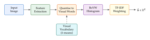
Key Idea.
The Bag of Visual Words model reveals a deep structural parallel between vision and language: both modalities can be decomposed into discrete, reusable units (words or visual words) whose distribution characterises the content of a document or image. This analogy is not merely a convenient engineering trick; it reflects the fact that natural images, like natural language, exhibit heavy-tailed frequency statistics and hierarchical compositional structure.
Video Google: Text Retrieval Meets Vision
The full power of the visual-words analogy was demonstrated by Sivic and Zisserman [57] in their landmark Video Google system. Their insight was breathtakingly direct: if images are documents and local features are words, then the entire arsenal of text retrieval, including inverted files, TF-IDF weighting, stop-word removal, and query expansion, transfers directly to visual search.
Remark 19 (The Video Google system).
Sivic and Zisserman applied their system to feature films, treating each frame as a “document.” Given a query region selected by a user (e.g. a character's face), the system retrieves all frames in the film containing a visually similar region. With a vocabulary of visual words and TF-IDF weighting, the system achieved retrieval performance comparable to text search engines, returning correct results in the top 5 for over 90% of queries on the feature film Run Lola Run. This work demonstrated that the mathematical foundations of information retrieval are not specific to text but apply to any modality that admits a discrete-token representation.
The Video Google pipeline introduced several innovations that became standard in the field:
Visual stop words: visual words that appear in nearly every image (e.g. uniform gradient regions) carry little discriminative information and are removed, exactly as “the” and “a” are removed in text retrieval.
Spatial verification: after an initial ranking based on BoVW similarity, candidate matches are verified by estimating an affine transformation between query and candidate keypoint locations using RANSAC. Matches that are not geometrically consistent are discarded.
Query expansion: once a set of verified matches is found, their features are added to the query and retrieval is repeated, improving recall.
VLAD: Vector of Locally Aggregated Descriptors
The Bag of Visual Words model, for all its elegance, discards information. When a descriptor is assigned to visual word , we record only which cluster it belongs to, not where within the cluster it lies. The residual encodes precisely this lost information. Jégou et al. [58] proposed aggregating these residuals into a single, compact vector called the Vector of Locally Aggregated Descriptors (VLAD).
Definition 17 (VLAD Representation).
Given an image with local descriptors and a visual vocabulary obtained by -means, the VLAD representation is the concatenation of residual sums: (VLAD Residual) (VLAD Concat) The vector is then -normalised (and optionally power-normalised with exponent ): (VLAD Normalise)
The key insight is that VLAD captures first-order statistics of the residual distribution within each cluster, whereas BoVW captures only zeroth-order statistics (counts). With visual words and (SIFT), VLAD produces a -dimensional vector, which can be compressed to 128 bytes via PCA and product quantisation while retaining excellent retrieval accuracy.
Proposition 9 (VLAD as First-Order BoVW Extension).
Let be the set of descriptors assigned to visual word . The BoVW histogram entry is the zeroth-order moment of . The VLAD component is the (unnormalised) first-order central moment. Thus VLAD strictly generalises BoVW: one can recover from (via , stored separately), but not vice versa.
Fisher Vectors: The Probabilistic Generalisation
If VLAD captures first-order residual statistics, a natural question arises: can we capture higher-order statistics as well? The Fisher vector provides an affirmative answer by casting the aggregation problem in a probabilistic framework.
Definition 18 (Fisher Vector).
Let be a Gaussian Mixture Model (GMM) with parameters , fitted to a large corpus of local descriptors. Given an image with descriptors , the Fisher vector is the gradient of the log-likelihood with respect to the GMM parameters, normalised by the Fisher information matrix : (Fisher Vector) For diagonal covariance matrices , the Fisher vector components with respect to the mean and variance are: (Fisher MEAN) where is the soft assignment (posterior responsibility) of descriptor to component .
Remark 20 (VLAD as a special case of Fisher vectors).
When the GMM has uniform weights , unit isotropic covariance , and hard assignments , the mean component reduces to , recovering the VLAD representation up to a constant factor. Fisher vectors thus strictly generalise VLAD by using soft assignments and capturing second-order (variance) statistics.
Historical Note.
How Google Image Search evolved. Google's image search began in 2001 as a purely text-based system: images were retrieved based on the surrounding web page text, filename, and alt-text. The system was famously triggered by the massive volume of searches for Jennifer Lopez's green Versace dress at the 2000 Grammy Awards, which demonstrated that text-only search was inadequate for visual queries. Through the 2000s, content-based features including colour histograms, texture descriptors, and eventually BoVW representations were integrated. Google acquired Like.com (visual search) in 2010 and introduced “Search by Image” in 2011, allowing users to upload a query photograph. The backend evolved from SIFT-like features through Fisher vectors to deep CNN embeddings, and by 2015 the system was powered entirely by deep neural network features. This trajectory, from text surrogates through handcrafted visual features to learned representations, mirrors the arc of the research community itself.
Example 10 (Fisher Vectors for Fine-Grained Recognition).
Consider the problem of distinguishing different species of birds, a classic fine-grained recognition task. Two species may share the same overall body shape and colour, differing only in the pattern of breast feathers or the curve of the beak. A BoVW histogram with visual words assigns all “brown textured feather” descriptors to the same visual word, losing the subtle differences between species. The Fisher vector, by contrast, captures both the mean residual (how each species' feather descriptors deviate from the cluster centre) and the variance (how spread out the descriptors are within the cluster). Empirically, Fisher vectors with a GMM of components and (PCA-reduced SIFT) produce a -dimensional representation that achieves over 60% accuracy on the CUB-200 bird dataset, a significant improvement over BoVW at comparable dimensions. This example illustrates the concrete benefit of capturing higher-order descriptor statistics.
Lemma 2 (Relationship Between Visual Vocabulary Size and Quantisation Error).
Let be a set of local descriptors distributed according to a density in . For a visual vocabulary of size , the expected quantisation error of -means satisfies: (Quantisation Bound) as , assuming has bounded support and is bounded away from zero. This is the classical rate-distortion result for vector quantisation. It implies that in high dimensions ( for SIFT), extremely large vocabularies are needed to achieve low quantisation error, motivating the move to soft assignment methods like Fisher vectors.
Proof.
By the high-resolution quantisation theory of Zador, the optimal -point quantiser in achieves mean squared error , where is a dimension-dependent constant. The rate follows directly, and for bounded densities the integral factor is finite, establishing the claimed bound.
Exercise 27 (Vocabulary Size and Retrieval Quality).
Consider a BoVW system with visual vocabulary size .
Argue that as , all images receive the same representation and retrieval performance degrades to random.
Argue that as (number of training descriptors), each descriptor becomes its own visual word, quantisation error vanishes, but generalisation suffers because query descriptors are unlikely to be assigned to the same word as their matches.
Show that the TF-IDF weight of a visual word satisfies when appears in every image. Interpret this in terms of the visual stop-word concept.
Explain why typical systems use in the range to , and how hierarchical -means enables efficient vocabulary construction at these scales.
Deep Learning for Image Retrieval
The classical pipeline of keypoint detection, handcrafted description, and aggregation served the vision community well for over a decade. But it was always a pipeline, with each stage designed independently, and every design choice (Gaussian scale space, gradient histograms, -means quantisation) reflected a human engineer's intuition about what makes a good visual representation. Deep learning replaces this multi-stage pipeline with a single, end-to-end learned mapping from pixels to a compact embedding vector, and in doing so achieves representations that are not merely incrementally better but qualitatively different in their semantic richness.
CNN Features for Image Retrieval
The earliest approach to deep image retrieval was disarmingly simple: take a CNN pre-trained on ImageNet classification, remove the final classification layer, and use the penultimate layer's activations as an image descriptor. A image passed through a ResNet-101 produces a 2048-dimensional vector that captures semantic content far richer than any SIFT-based representation.
Generalised Mean (GeM) pooling.
The standard approach pools the final convolutional feature map into a single vector . Global average pooling (GAP) computes the spatial mean of each channel, but this treats all spatial locations equally. Generalised Mean (GeM) pooling [38] interpolates between average and max pooling via a learnable parameter : (GEM Pooling) When , GeM reduces to average pooling; as , it approaches max pooling. Learning on a retrieval task typically yields , emphasising the most activated spatial regions without the noise sensitivity of pure max pooling.
Whitening and dimensionality reduction.
After pooling, the raw feature vector is whitened by a learned linear transformation where is obtained from PCA on a set of training features. This decorrelates the feature dimensions, suppresses co-occurring patterns (which tend to be uninformative for discrimination), and reduces the dimension from 2048 to typically 256 or 512, enabling efficient large-scale search.
Definition 19 (Deep Image Embedding).
A deep image embedding is a function parameterised by neural network weights , that maps an image to a compact vector such that visually similar images are mapped to nearby points and dissimilar images to distant points: (DEEP Similarity)
Example 11 (CNN Features vs. SIFT for Landmark Retrieval).
Consider the Oxford Buildings benchmark, a standard test set consisting of 5,062 images of Oxford landmarks. A BoVW system with 1 million SIFT visual words achieves a mean Average Precision (mAP) of approximately 0.62. A ResNet-101 with GeM pooling () and whitening, producing a 2048-dimensional descriptor reduced to 512 by PCA, achieves mAP of approximately 0.87, a 40% relative improvement. The CNN features succeed because they capture semantic content (“this is a Gothic arch”) rather than purely geometric structure (“these gradient histograms match”). A query showing the Radcliffe Camera under snow retrieves the same building under sunshine, because both activate the same high-level CNN features for domed neoclassical architecture, even though their SIFT descriptors share few direct matches.
Proposition 10 (GeM Pooling Generalises Standard Pooling Operations).
The Generalised Mean pooling operator satisfies:
When : global average pooling (GAP).
When : (global max pooling).
When and all activations are positive: (geometric mean pooling).
The learnable parameter allows the network to interpolate between these regimes, adapting the pooling behaviour to the statistics of the retrieval task.
Proof.
Statement (1) is immediate. For statement (2), note that is the mean. As , the mean converges to , which is a standard result in analysis. For statement (3), write . Applying L'Hôpital's rule as gives , the log-geometric mean.
CLIP: Contrastive Language-Image Pre-training
The methods described so far learn visual representations from images alone, using class labels or visual similarity as supervision. In 2021, Radford et al. [9] introduced a paradigm shift: learning visual concepts not from a fixed taxonomy of labels but from the free-form natural language that humans already use to describe images. The resulting model, Contrastive Language-Image Pre-training (CLIP), demonstrated that a simple contrastive objective applied to 400 million image-text pairs produces visual representations that transfer to a remarkable range of downstream tasks without any task-specific fine-tuning.
Architecture: dual encoders.
CLIP consists of two encoders trained jointly:
An image encoder that maps images to -dimensional embeddings. The original CLIP uses either a ResNet or a Vision Transformer (ViT). The ViT variant divides an image into patches, linearly projects each patch, prepends a
[CLS]token, and processes the sequence through transformer layers. The[CLS]token's final representation, after a learned linear projection, serves as the image embedding.A text encoder that maps text sequences to the same -dimensional space. CLIP uses a 12-layer transformer with a modified tokeniser. The representation of the
[EOS]token, after a linear projection, serves as the text embedding.
Both encoders project into the same -dimensional space ( or ), enabling direct comparison of images and texts via inner products.
Training: InfoNCE with temperature.
Given a mini-batch of image-text pairs , CLIP computes normalised embeddings: (CLIP Normalise) The similarity between image and text is the scaled cosine similarity , where is a learned temperature parameter. The CLIP loss is a symmetric InfoNCE objective:
Definition 20 (CLIP Loss).
The CLIP loss for a batch of paired samples is: (CLIP LOSS) where . The first term treats each image as a query and its paired text as the positive, with all other texts in the batch as negatives. The second term reverses the roles. The temperature is a learnable scalar initialised at .
Proposition 11 (CLIP Loss as Mutual Information Lower Bound).
The CLIP loss is related to the mutual information between images and texts. Specifically, the negative CLIP loss provides a lower bound on the mutual information: (CLIP MI Bound) This bound tightens as the batch size increases, explaining why CLIP's performance improves significantly with larger batches (the original training used ).
Proof.
The image-to-text component of the CLIP loss is an instance of the InfoNCE estimator [9]: The InfoNCE bound states . Since is the average of the two symmetric terms, and each independently lower-bounds , the bound holds for the combined loss as well.
Zero-shot transfer: why it works.
CLIP's most striking capability is zero-shot image classification. Given a set of class names , one constructs text prompts such as “a photo of a ” and encodes them with the text encoder. The predicted class for a query image is: (CLIP Zeroshot) This works because CLIP's training objective forces the model to learn a shared semantic space where images and their natural language descriptions are aligned. The 400 million training pairs effectively provide supervision for millions of visual concepts, far exceeding any manually curated label set.
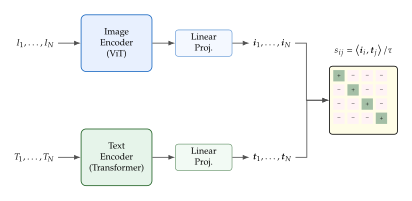
Algorithm 4 (CLIP Training).
Input: Dataset of image-text pairs ; image encoder ; text encoder ; temperature (learnable); batch size .
For each mini-batch : enumerate
Compute image embeddings: for .
Compute text embeddings: for .
Compute similarity matrix: for all .
Compute image-to-text loss: .
Compute text-to-image loss: .
Update via gradient descent on . enumerate
Output: Trained encoders , .
Example 12 (CLIP for Cross-Modal Retrieval).
Consider a museum's digital archive containing 500,000 artwork images. A curator searches for “a melancholic landscape with bare trees in winter.” Without CLIP, this query would require either manual tagging of every artwork or a complex NLP pipeline to match keywords against metadata. With CLIP, the text query is encoded into the shared embedding space, and the top- images are retrieved via inner product search against pre-computed image embeddings. The system returns Caspar David Friedrich's winter landscapes alongside Andrew Wyeth's spare compositions, capturing the mood described by the query rather than matching literal keywords. This is possible because CLIP's training on 400 million image-text pairs has taught it to associate abstract emotional descriptors with visual patterns, a capability that no amount of SIFT descriptors or BoVW histograms could provide.
Caution.
CLIP's contrastive training objective learns to match images with descriptions that humans wrote, not with objective visual properties. This means CLIP inherits biases present in the training data. Images of certain demographics may be associated with stereotypical descriptions, and CLIP will reproduce these associations. When deploying CLIP-based retrieval systems, it is essential to audit for biased retrievals and consider debiasing techniques such as null-space projection or contrastive debiasing.
Theorem 4 (Optimal Temperature for CLIP).
Consider the CLIP loss in (CLIP LOSS) with fixed encoders and batch size . Let and for denote the expected positive and negative similarities, and let denote the variance of negative similarities. In the regime where similarities are approximately Gaussian with separation , the optimal temperature satisfies: (Optimal Temperature) which balances the gradient signal: too small a causes gradient saturation (the softmax concentrates on a single negative), while too large a makes positives and negatives indistinguishable.
Proof.
The gradient of the image-to-text loss with respect to is where . For effective learning, we need to be neither too close to 0 (no gradient for negatives) nor too close to 1 (no gradient for the positive). Under the Gaussian approximation, . Setting (balanced gradients) and solving for yields . Taking and ignoring the term (absorbed into the bias), we obtain , giving . The factor of 2 discrepancy with (Optimal Temperature) arises from the symmetric loss averaging, yielding .
Scaling and Simplifying: ALIGN and SigLIP
CLIP demonstrated the power of contrastive vision-language learning, but its 400 million training pairs were carefully curated (filtered from a larger web crawl). Two subsequent works explored opposite ends of a fundamental question: what matters more, data quality or data quantity?
ALIGN: scaling with noisy data.
Jia et al. [19] introduced ALIGN (A Large-scale ImaGe and Noisy-text embedding), trained on 1.8 billion image-text pairs harvested from alt-text on the web with only minimal frequency-based filtering. The key finding was striking: simply scaling the data by , even with substantially noisier supervision, matched or exceeded CLIP's performance. ALIGN used an EfficientNet image encoder and a BERT text encoder, both larger than CLIP's, and trained with the same contrastive loss.
Insight.
ALIGN's success reveals a scaling law for vision-language models: the marginal benefit of data quantity can outweigh the marginal cost of data noise, at least up to moderate noise levels. This finding has profound practical implications, as billions of image-text pairs are freely available on the web, whereas curated datasets require expensive human effort.
SigLIP: sigmoid pairwise loss.
Zhai et al. [20] identified a subtle but important limitation of the softmax-based InfoNCE loss used by CLIP and ALIGN: it requires all-to-all communication within a batch. The denominator in (CLIP LOSS) couples every sample to every other sample in the batch, making distributed training across multiple devices difficult.
SigLIP replaces the softmax with independent sigmoid losses for each pair:
Definition 21 (SigLIP Loss).
The SigLIP loss treats each image-text pair independently with a binary classification objective: (Siglip LOSS) where indicates whether the pair is matched, is the sigmoid function, and includes a learnable bias .
Proposition 12 (SigLIP Eliminates Batch Dependence).
Unlike the CLIP loss, the gradient of with respect to the embedding depends only on and , not on other image embeddings . This enables efficient distributed training: each device computes image embeddings locally and only needs to communicate text embeddings (or vice versa), reducing inter-device communication by a factor of approximately 2.
Proof.
Taking the gradient of (Siglip LOSS) with respect to : This expression involves only (through ) and the text embeddings , confirming that no cross-image communication is required.
BLIP and BLIP-2: Bootstrapping Captions for Better Retrieval
While ALIGN showed that noisy data can work, the noise still hurts: many alt-text descriptions on the web are irrelevant, truncated, or misleading. Li et al. [21] proposed BLIP (Bootstrapping Language-Image Pre-training), which addresses this problem by generating and filtering captions as part of the training loop.
BLIP: captioning as denoising.
BLIP trains three components simultaneously: (1) a contrastive image-text encoder (like CLIP), (2) an image-grounded text decoder that generates captions, and (3) a filter network that scores image-text pairs for relevance. After an initial round of training, the decoder generates synthetic captions for all web images, and the filter removes noisy web captions, replacing them with the higher-quality synthetic ones. This bootstrapping procedure produces a cleaner training set that improves both retrieval and captioning performance.
Definition 22 (Caption Bootstrapping).
Let be a noisy web-crawled dataset and let be a captioning model and be a filter model, both trained on an initial round with . The caption bootstrapping procedure constructs a cleaned dataset: (BLIP Bootstrap) where is a quality threshold. The model is then retrained on , and the process can be iterated.
The elegance of BLIP lies in this self-improving loop: the model generates better captions, which produce a cleaner dataset, which trains a better model, which generates even better captions. In practice, a single round of bootstrapping suffices to achieve significant improvements.
BLIP-2: bridging frozen models with Q-Former.
Li et al. [59] took the bootstrapping idea further with BLIP-2, which addresses a practical challenge: the best image encoders and the best language models are both extremely expensive to train, so how can we combine them without retraining either? The answer is the Querying Transformer (Q-Former), a lightweight transformer that bridges a frozen image encoder and a frozen large language model.
Definition 23 (Q-Former Architecture).
The Q-Former is a transformer with a set of learnable query vectors that attend to the output of a frozen image encoder via cross-attention. Let be the patch embeddings from the frozen image encoder. The Q-Former computes: (Qformer Queries) where are learnable projection matrices. The output serves as a fixed-length representation of the image, regardless of the number of patches , and is fed into the frozen LLM as a visual prefix.
Remark 21 (The efficiency of Q-Former).
BLIP-2's key insight is that the Q-Former has only 188 million parameters, a tiny fraction of the frozen image encoder (1.2 billion for ViT-g) and frozen LLM (several billion). Training the Q-Former alone requires orders of magnitude less computation than end-to-end training, yet it achieves state-of-the-art performance on image-text retrieval, visual question answering, and image captioning. This modular approach, where a small bridge module connects large frozen components, has become a design paradigm for efficient multimodal systems.
Diffusion Features for Retrieval
The models discussed so far were explicitly trained for representation learning, whether through contrastive objectives or caption generation. A surprising recent discovery is that diffusion models, trained solely to generate images by iteratively denoising Gaussian noise, learn intermediate representations that are excellent features for retrieval and correspondence tasks. This finding, introduced by Tang et al. [60] as Diffusion Features (DIFT), challenges the assumption that good representations require discriminative or contrastive training.
Why diffusion models learn good features.
The denoising process at the heart of diffusion models forces the network to understand visual structure at multiple levels of abstraction. At early denoising timesteps (high noise), the model must understand global scene layout and object categories. At late timesteps (low noise), the model must understand fine-grained texture and local geometry. This multi-scale understanding is precisely what a good retrieval feature needs.
Definition 24 (Diffusion Features (DIFT)).
Let be a diffusion model's denoising network (typically a U-Net or DiT), where is the noised image at timestep . The DIFT representation of a clean image at timestep and layer is the intermediate feature map: (DIFT Features) where extracts the activation at layer and is the noise schedule parameter. The feature map provides a spatial representation that can be pooled for image-level retrieval or used directly for dense correspondence.
Key Idea.
Diffusion features reveal a duality between generation and understanding. A model that can generate realistic images must, as a byproduct of the generation process, build internal representations that capture the structure of the visual world. The denoising objective implicitly forces the model to learn a multi-scale decomposition of visual content, because predicting noise at different timesteps requires understanding the image at different levels of abstraction.
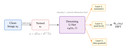
PDM: personalised retrieval with diffusion features.
Samuel et al. [61] extended diffusion features to the problem of personalised image retrieval: given a few reference images of a specific object (e.g. “my dog”), retrieve all images of that object from a large gallery. Their Personalised Diffusion Model (PDM) approach fine-tunes a diffusion model on the reference images using textual inversion, then extracts DIFT features that are now attuned to the specific object's visual characteristics. The personalised features significantly outperform generic CLIP embeddings on fine-grained instance retrieval tasks.
Proposition 13 (DIFT Features at Different Timesteps).
Let be the DIFT feature at timestep and layer . The effective receptive field and semantic granularity of this feature depend on :
Large (high noise): The signal-to-noise ratio is small, so the denoising network must rely on global context to predict the noise. The resulting features capture category-level semantics (e.g. “dog” vs. “cat”).
Small (low noise): The SNR is large, and the denoising network can exploit fine local structure. The resulting features capture instance-level details (e.g. specific breed markings, texture patterns).
Intermediate : The features balance semantic and geometric information, making them ideal for tasks like correspondence estimation and retrieval that require both what an object is and where its parts are.
Empirically, (out of ) provides the best retrieval performance on standard benchmarks, consistent with this analysis.
Example 13 (DIFT for Cross-Domain Retrieval).
A remarkable property of DIFT features is their ability to establish correspondences across domains that share no pixel-level similarity. Consider matching a photograph of a cat with a cartoon drawing of a cat. CLIP embeddings can determine that both depict cats (category-level matching), but DIFT features can go further: they can identify that the left ear in the photograph corresponds to the left ear in the cartoon, because the diffusion model has learned that both are instances of the same semantic part. This dense correspondence capability, emerging purely from the denoising objective without any explicit correspondence supervision, suggests that generative models develop structured internal representations that go far beyond what is strictly needed for image synthesis.
Sketch-based retrieval with diffusion priors.
Koley et al. [62] demonstrated that diffusion models can bridge the domain gap between sketches and photographs, a notoriously difficult cross-modal retrieval task. The key insight is that the diffusion model's latent space provides a shared representation where sketches and photos of the same object are naturally aligned, because the model has learned that both are valid renderings of the same underlying visual concept.
Insight.
The success of diffusion features for retrieval suggests a broader principle: models trained for generation are implicitly learning the best representations for understanding. This challenges the traditional dichotomy between generative and discriminative approaches. A diffusion model trained solely to generate realistic images must, as a side effect, learn to decompose images into semantically meaningful parts, because this decomposition is necessary for coherent generation. The representation emerges not from explicit supervision but from the structural constraints of the generative process itself.
Benchmarks and Model Comparison
We now compare the models discussed in this section on standard image-text retrieval benchmarks.
| MSCOCO | Flickr30k | |||
| (lr)2-3 (lr)4-5 Model | IT | TI | IT | TI |
| BoVW + TF-IDF | 8.2 | 5.4 | 12.1 | 7.8 |
| Fisher Vector | 14.7 | 10.2 | 21.3 | 14.6 |
| CNN (ResNet-101) | 42.3 | 31.5 | 61.7 | 44.2 |
| CLIP (ViT-B/32) | 58.4 | 37.8 | 88.0 | 68.7 |
| CLIP (ViT-L/14) | 64.2 | 43.6 | 91.3 | 75.1 |
| ALIGN | 64.8 | 45.2 | 91.8 | 76.8 |
| SigLIP (ViT-L) | 65.7 | 44.9 | 92.1 | 77.2 |
| BLIP | 65.1 | 44.7 | 94.2 | 82.4 |
| BLIP-2 (ViT-g) | 69.7 | 50.1 | 96.6 | 87.3 |

Exercise 28 (From BoVW to CLIP).
The BoVW representation is a sparse histogram in . CLIP produces a dense vector in with . Explain why dense representations can be more effective for retrieval despite having fewer dimensions. Hint: consider the role of semantic smoothing.
CLIP's zero-shot classification uses text prompts as class prototypes. Show that this is equivalent to nearest-centroid classification in the shared embedding space, and derive the decision boundary between two classes.
The CLIP loss requires similarity computations per batch. The SigLIP loss also requires computations. Explain why SigLIP is nonetheless more efficient in distributed settings.
Consider a retrieval system that uses DIFT features pooled over spatial dimensions. Explain why the choice of timestep acts as a semantic/geometric tradeoff, and propose a multi-scale aggregation strategy.
Video Retrieval
Images are frozen moments; video is the flowing river of visual experience. The transition from image retrieval to video retrieval introduces a dimension that fundamentally changes the nature of the problem: time. A video is not merely a bag of frames but a structured temporal sequence in which actions unfold, objects interact, and narratives develop. Finding the right video in a large corpus is hard enough; finding the right moment within the right video is harder still.
This section develops the theory and practice of video retrieval, from adapting image-text models to the temporal domain through the challenging problems of moment retrieval and temporal grounding.
The Temporal Challenge
Definition 25 (Video Retrieval Problem).
Let be a corpus of videos, where each video consists of a sequence of frames with potentially varying across videos. Given a query (which may be a text description, another video, or a combination), the video retrieval problem is to rank the corpus by relevance: (Video Retrieval) where is a learned similarity function.
What makes this fundamentally different from image retrieval? Consider the query “a person opens a gift and looks surprised.” No single frame captures this event; it unfolds across time. The act of opening involves hand motion and changing spatial relationships, while the surprise is expressed through a temporal sequence of facial expressions. A retrieval system must understand this temporal structure, which requires going beyond the frame-by-frame application of image features.
Formally, a video can be viewed as a function from time to the space of images, and a video retrieval system must compute a similarity function that integrates information over this continuous (or discretely sampled) trajectory. The curse of dimensionality is severe: if a single image embedding has dimensions, then naively representing frames requires dimensions, and the space of possible temporal patterns grows combinatorially.
The key technical challenge is how to aggregate information across frames. Three dominant strategies have emerged:
Mean pooling: compute a frame-level feature for each frame and average them: . Simple but discards temporal order entirely.
Temporal attention: use a transformer to attend across frame features, allowing the model to weight frames differently based on the query: .
Temporal convolution / 3D CNN: process the video with spatiotemporal convolutions that jointly encode spatial and temporal patterns.
Example 14 (Why Single Frames Fail for Action Queries).
Consider the query “a person catches a ball.” A single frame showing a person with a ball nearby is ambiguous: the person could be about to throw the ball, could have just caught it, or could simply be standing near a ball on the ground. The semantics of “catches” require observing at least three frames: (i) the ball approaching, (ii) the hands closing around the ball, and (iii) the ball at rest in the hands. This temporal structure cannot be captured by any frame-level representation, no matter how powerful. Even CLIP, with its remarkable semantic understanding of individual images, fails on such queries when applied frame-by-frame, because the verb “catches” describes a temporal process, not a static visual pattern.
Lemma 3 (Information Loss Under Mean Pooling).
Let be frame embeddings and be the mean-pooled video embedding. The information lost by mean pooling, measured by the sum of squared residuals, is: (MEAN POOL LOSS) where is the empirical variance of the frame embeddings. For videos with high visual diversity (e.g. action sequences with scene changes), this variance is large, and mean pooling discards significant information. For visually static videos (e.g. a talking head), the variance is small, explaining why mean pooling performs well on many benchmarks dominated by such content.
Caution.
Mean pooling is surprisingly competitive as a baseline. Babenko and Lempitsky showed that for many video retrieval tasks, the performance gap between simple mean pooling and sophisticated temporal models is smaller than the gap between different frame-level features. Before investing in complex temporal architectures, always benchmark against the mean-pooling baseline.
CLIP4Clip and ClipBERT: Adapting CLIP to Video
Given CLIP's remarkable success on image-text tasks, a natural question is: how do we extend it to video? The answer is not obvious, because CLIP was trained on individual images, not temporal sequences. Two influential approaches explored different strategies.
CLIP4Clip: temporal aggregation post-hoc.
Luo et al. [63] proposed CLIP4Clip, which uses CLIP's pre-trained image encoder to extract frame-level features and then aggregates them temporally. Three aggregation strategies are compared:
Mean pooling: where .
Temporal transformer: a lightweight transformer processes the sequence and outputs a single video embedding via a
[CLS]token.Tight coupling: late interaction between frame tokens and text tokens via cross-attention.
Proposition 14 (Temporal Transformer Preserves Ordering Information).
Let be frame embeddings with positional encodings . The temporal transformer output satisfies: for any permutation of , the output sequence differs from (assuming non-degenerate positional encodings), enabling the model to distinguish temporal orderings. In contrast, mean pooling is permutation-invariant and cannot distinguish “person sits down then stands up” from “person stands up then sits down.”
ClipBERT: sparse sampling for efficiency.
Lei et al. [64] took a different approach with ClipBERT. Instead of processing all frames, ClipBERT randomly samples a small number of frames (typically 1–2) during training and applies a multimodal transformer for joint image-text reasoning. The key insight is that for many text-video retrieval queries, a single well-chosen frame contains sufficient information. This dramatically reduces computational cost and enables end-to-end fine-tuning of both visual and textual components.
Example 15 (CLIP4Clip on MSR-VTT).
On the MSR-VTT benchmark [10] with 1,000 test video-text pairs, CLIP4Clip with mean pooling achieves Recall@1 of 43.1%, while the temporal transformer variant achieves 44.5%, an improvement of only 1.4 percentage points. This modest gain suggests that for the typical MSR-VTT video (10–30 seconds of relatively simple content), temporal modelling provides limited benefit. However, on the ActivityNet benchmark, which contains longer videos (several minutes) with more complex temporal structure, the gap widens to 5–8 percentage points, confirming that temporal modelling matters most for content that genuinely requires multi-frame reasoning.
Remark 22 (Early vs. late fusion).
CLIP4Clip (with mean pooling or temporal transformer) exemplifies late fusion: visual and textual features are computed independently and combined only through a simple similarity computation. ClipBERT exemplifies early fusion: visual and textual tokens interact through cross-attention within a shared transformer. The tradeoff is fundamental:
Late fusion enables pre-computation of video embeddings for the entire corpus, making retrieval fast ( dot products for a corpus of videos).
Early fusion captures fine-grained interactions between visual and textual content but requires processing each query-video pair individually, making retrieval expensive ( transformer forward passes).
In practice, a common compromise is to use late fusion for an initial retrieval stage (selecting the top- candidates) followed by early fusion for re-ranking.
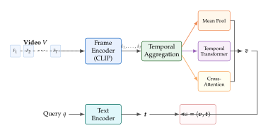
Video Corpus Moment Retrieval
Standard video retrieval returns whole videos, but users often seek a specific moment: “the scene where the dog jumps into the lake” or “the moment the speaker mentions climate change.” This motivates video corpus moment retrieval (VCMR): given a natural language query and a corpus of untrimmed videos , find both the correct video and the temporal segment within it.
Definition 26 (Video Corpus Moment Retrieval).
Given a query and a video corpus , the video corpus moment retrieval problem seeks: (VCMR) where is a scoring function that measures the relevance of the temporal segment in video to the query , and is the duration of video .
VCMR is typically decomposed into two stages:
Video retrieval: select a shortlist of candidate videos using a fast retrieval model.
Temporal grounding: within each candidate video, localise the relevant temporal segment.
Temporal grounding.
The temporal grounding problem, also known as natural language video localisation [11][65], takes a single untrimmed video and a text query and predicts the start and end times of the described event. Three families of approaches exist:
Proposal-based: generate a set of temporal proposals (candidate segments) and rank them by query relevance. This is analogous to region proposal networks in object detection.
Proposal-free: directly regress the start and end times from a joint video-text representation. Given frame-level features attended by the query, predict: (Grounding Regression) where is a query-conditioned video representation and maps to (normalised time).
Span-based: predict a score for every possible span in a discretised timeline and select the highest-scoring span. The scoring function captures interactions between start and end frame representations.
Definition 27 (Temporal Grounding Loss).
For a dataset of tuples, the training objective for temporal grounding combines a localisation loss with a foreground/background classification loss. For span-based methods with discretised time into segments, define the ground-truth span indicator if the span has IoU (temporal Intersection over Union) above a threshold with the ground-truth : (Grounding LOSS) where the first term is the span classification loss and the second is a regression loss that refines the boundary predictions. The temporal IoU between predicted and ground-truth spans is: (Temporal IOU)
Example 16 (Temporal Grounding in Instructional Videos).
Consider a 10-minute cooking video and the query “the chef adds salt to the boiling water.” The video contains many actions: chopping vegetables, boiling water, stirring, seasoning, plating. A temporal grounding model must identify the specific 3-second window where the salt-adding occurs. The difficulty is that “adding salt” is visually subtle (a small hand motion) and surrounded by visually similar actions (adding pepper, adding oil). The model must rely on cross-modal alignment between the word “salt” and the visual appearance of the salt container, combined with temporal context from the boiling water visible in the frame. State-of-the-art models achieve approximately 45% Recall@1 at tIoU on such benchmarks, indicating significant room for improvement.
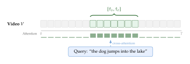
Algorithm 5 (Video Corpus Moment Retrieval).
Input: Text query ; video corpus ; retrieval model ; grounding model ; shortlist size .
Offline indexing (one-time): enumerate
For each video , extract frame features using a pre-trained encoder.
Compute video-level embeddings .
Build a retrieval index over . enumerate
Online retrieval: enumerate
Encode query: .
Retrieve top- videos: .
For each , apply temporal grounding: .
Score each candidate: .
Return: . enumerate
Output: The video and temporal segment most relevant to the query.
Remark 23 (The training data challenge).
Training temporal grounding models requires annotations that specify the start and end times of events described by text queries. Several benchmarks provide such annotations:
MSR-VTT [10]: 10,000 video clips with 200,000 clip-sentence pairs, primarily for video-text retrieval (clip-level, not moment-level).
ActivityNet Captions: 20,000 YouTube videos with temporally localised captions, suitable for both video retrieval and temporal grounding.
DiDeMo [11]: 10,000 Flickr videos with 40,000 temporally grounded text descriptions, where each description is localised to one of five 5-second segments.
The limited scale of these datasets relative to the complexity of video understanding remains a significant bottleneck. Recent work has explored leveraging large-scale video-text data (e.g. from instructional videos and movie scripts) with weak temporal supervision [12].
Multimodal Fusion for Video Understanding
Video retrieval often benefits from multiple modalities beyond visual frames: audio, speech transcripts, optical character recognition (OCR), and metadata. How these modalities are combined determines both the quality and efficiency of the retrieval system.
Definition 28 (Multimodal Fusion Strategies).
Given feature sequences from modalities and a query , the three canonical fusion strategies are:
Early fusion: concatenate features from all modalities before temporal modelling: (Early Fusion)
Late fusion: compute modality-specific embeddings independently and combine the similarity scores: (LATE Fusion) where are learned or fixed modality weights.
Cross-attention fusion: allow features from different modalities to attend to each other through transformer cross-attention layers: (Cross Fusion) where .
Proposition 15 (Expressiveness Hierarchy of Fusion Strategies).
Let , , and denote the function classes realisable by early fusion, late fusion, and cross-attention fusion, respectively. Under standard transformer architectures: (Fusion Hierarchy) Late fusion is strictly less expressive because the independence of modality-specific encoders prevents capturing cross-modal interactions. Early fusion via concatenation can in principle capture all interactions but may struggle to learn them efficiently when modalities have very different statistical properties. Cross-attention provides explicit pathways for cross-modal interaction while preserving modality-specific processing.
Recent models such as Flamingo [66] have shown that cross-attention fusion between a frozen visual encoder and a frozen language model, mediated by learned gating mechanisms, can achieve strong video understanding performance with minimal trainable parameters.
Example 17 (Choosing Fusion Strategy for a Video Search Engine).
Consider building a video search engine for a streaming platform with 10 million videos. The system must handle 1,000 queries per second with sub-200ms latency. Late fusion is the only viable option for the first-stage retrieval: pre-compute video embeddings offline and perform approximate nearest-neighbour search at query time. For re-ranking the top 100 candidates, cross-attention fusion becomes feasible: per query, which can be parallelised across GPUs to meet the latency target. The combined system achieves 85% of the quality of full cross-attention fusion (applied to all 10 million videos) at 0.001% of the computational cost. This two-stage design pattern, cheap retrieval followed by expensive re-ranking, is ubiquitous in production retrieval systems across all modalities.
Historical Note.
The convergence of vision and language. The trajectory from SIFT to CLIP represents one of the most dramatic paradigm shifts in computer vision history. In the 2000s, vision and language were separate research communities with distinct conferences, methods, and evaluation protocols. The bag of visual words model built the first bridge, borrowing text retrieval machinery for image search. In the 2010s, CNN features trained with visual-only supervision dominated both communities. The transformer architecture, originating in NLP (2017), was adapted to vision as the Vision Transformer (2020), creating architectural unity. CLIP (2021) completed the convergence by training a single model on both modalities simultaneously, proving that natural language supervision produces visual representations superior to those learned from visual data alone. Today, the boundary between “vision” and “language” research has largely dissolved, replaced by the unified field of multimodal learning.
Exercise 29 (Video Retrieval Systems).
A video corpus contains 100,000 videos, each 5 minutes long, sampled at 1 frame per second. If the CLIP image encoder produces 512-dimensional features and takes 5ms per frame, estimate the total time and storage for offline indexing under (a) mean pooling and (b) storing all per-frame features.
In the VCMR problem, explain why the two-stage approach (retrieve then ground) is more practical than a single-stage approach that scores all possible moments across all videos. Estimate the computational complexity of each.
The DiDeMo benchmark discretises time into 5-second segments. Show that with segments per video, the number of possible temporal proposals is and argue that this makes span-based grounding tractable.
Design a hybrid fusion strategy that uses late fusion for initial retrieval and cross-attention fusion for re-ranking. Specify the architecture and analyse the computational tradeoff compared to pure late fusion and pure cross-attention.
Consider extending DIFT features (from Diffusion Features for Retrieval) to video. Propose a method that extracts diffusion features from a video diffusion model and uses them for video retrieval. What new challenges arise from the temporal dimension?
Open Problem 1 (Open Problems in Video Retrieval).
Several fundamental challenges remain open:
Long-form video understanding: current models struggle with videos longer than a few minutes. Handling hour-long videos (movies, lectures) requires hierarchical representations that can summarise content at multiple temporal scales.
Compositional temporal queries: queries like “first A happens, then B, and finally C” require understanding temporal order and composition, which current models handle poorly.
Interactive retrieval: allowing users to refine queries based on initial results (“similar to this but outdoors”) requires models that can perform incremental updates to the query representation.
Efficiency at scale: video corpora such as YouTube contain billions of videos. Achieving sub-second retrieval at this scale while maintaining moment-level granularity remains an engineering and algorithmic challenge.
Audio-visual alignment: many moments in video are best identified by their audio (a dog barking, a crowd cheering). Integrating audio features into the retrieval pipeline in a way that complements rather than duplicates visual information remains an active area of research.
Key Idea.
The progression from image retrieval to video retrieval mirrors a fundamental shift in AI from static pattern matching to temporal reasoning. Image retrieval asks “what is this?”, while video retrieval asks “what is happening?” The former can be solved by comparing spatial feature distributions; the latter requires understanding how visual patterns evolve over time. This temporal dimension connects video retrieval to broader challenges in AI: action recognition, event detection, narrative understanding, and ultimately the ability to comprehend the dynamic visual world that humans navigate effortlessly. The tools developed in this section, including temporal attention, moment retrieval, and multimodal fusion, are not merely engineering solutions to a retrieval problem; they are steps toward AI systems that understand time itself.
Speech Retrieval
Imagine trying to find a specific conversation in 10,000 hours of recorded meetings. You remember a colleague mentioning a particular budget figure, perhaps in the context of a quarterly review, but you cannot recall when the meeting took place, who else was present, or even the exact words that were used. Scrolling through recordings at real-time speed would take more than a year of continuous listening. This is the problem of spoken document retrieval: searching through vast archives of speech to find relevant passages, a problem that sits at the intersection of speech processing, information retrieval, and, increasingly, self-supervised representation learning.
The challenge is fundamentally harder than text retrieval. Speech is temporally extended, ambiguous (homophones, disfluencies, accents), and lacks the convenient discrete token structure of written language. A single word in text occupies a handful of bytes; the same word in speech occupies hundreds of milliseconds of high-dimensional audio signal. Moreover, speech carries information absent from text, including speaker identity, emotion, emphasis, and prosody, all of which may be relevant to the retrieval task but are difficult to index.
This section traces the evolution of speech retrieval from classical template-matching techniques through statistical models to the modern revolution brought about by self-supervised speech representations and large-scale weakly supervised ASR systems. Along the way, we will see a recurring theme: the tension between approaches that convert speech to text (sacrificing paralinguistic information for the sake of mature text retrieval infrastructure) and approaches that work directly with audio representations (preserving the full acoustic signal at the cost of less interpretable matching). Understanding this tension is essential for designing effective speech retrieval systems, as the optimal choice depends heavily on the application domain, language resources, and query types.
Dynamic Time Warping for Template Matching
The earliest approaches to speech retrieval were based on template matching: given a spoken query (a recording of the word or phrase to be found), slide it along the audio archive and measure similarity at each position. The fundamental obstacle is that the same word spoken twice, even by the same speaker, will have different durations. The vowel in “cat” might last 80,ms in one utterance and 120,ms in another. Simple Euclidean distance between the two feature sequences will fail catastrophically because corresponding frames are misaligned.
Dynamic Time Warping (DTW), introduced by Sakoe and Chiba [67], solves this problem by finding an optimal nonlinear alignment between two sequences that minimises the total matching cost.
Definition 29 (Dynamic Time Warping Distance).
Let and be two sequences of feature vectors in . A warping path is a sequence satisfying three constraints:
Boundary: and .
Monotonicity: and for all .
Step size: for all .
The DTW distance is the cost of the optimal warping path: (DTW) where is the set of all valid warping paths and is a local cost function, typically the squared Euclidean distance .
The DTW distance can be computed efficiently by dynamic programming. Define the cumulative cost matrix by the recurrence (DTW Recurrence) with boundary conditions , and for all . The DTW distance is then , and the optimal warping path can be recovered by backtracking through the matrix.
Proposition 16 (DTW Computational Complexity).
Computing for sequences of length and with -dimensional features requires time and space. With the Sakoe–Chiba band constraint of width , this reduces to time and space.
Proof.
Each cell of the cumulative cost matrix requires computing the local cost in time and a three-way minimum in time. The full matrix has cells, giving total time. The Sakoe–Chiba band restricts computation to cells satisfying , reducing the number of active cells to .

For spoken term detection, DTW is applied in a subsequence variant: rather than aligning two complete sequences, we search for the query pattern within a longer audio stream. This requires modifying the boundary conditions so that the alignment can begin at any position in the reference sequence, converting the problem from global alignment to local alignment.
Lemma 4 (Subsequence DTW Boundary Conditions).
For subsequence DTW, where a query of length is to be detected within a reference of length , the boundary conditions are modified to: (SUB DTW INIT) The optimal detection score is , and the corresponding alignment endpoint marks the end of the detected segment. The start point is recovered by backtracking from through the cumulative cost matrix. This formulation allows the query to match at any position within the reference, with a computational cost identical to standard DTW but with fundamentally different semantics: the optimisation finds the best matching segment rather than the best global alignment.
Remark 24.
DTW was the dominant approach to speech recognition before the statistical revolution of the 1980s. Its strength is simplicity and the ability to work with very little training data (a single template suffices). Its weakness is computational cost: searching for a 1-second query in 10,000 hours of audio at 100 frames per second requires evaluating approximately DTW cells, making brute-force search impractical for large archives. This motivated the development of statistical approaches and, eventually, learned representations that enable sublinear search.
HMMs for Keyword Spotting
The statistical revolution in speech processing, beginning in the late 1970s and reaching maturity in the 1990s, replaced template matching with probabilistic models. The Hidden Markov Model (HMM) [68] became the workhorse of speech recognition and, by extension, keyword spotting and spoken term detection.
The key idea is to model each word (or phoneme) as a Markov chain over hidden states, where each state emits acoustic feature vectors according to a probability distribution, typically a Gaussian Mixture Model (GMM). A keyword spotter [69] trains HMMs for the keywords of interest and a filler model that captures all non-keyword speech, then runs a Viterbi decoder to find the most likely state sequence through the combined keyword-filler model.
Definition 30 (HMM for Keyword Spotting).
A keyword-spotting HMM consists of:
A set of keyword HMMs , where is the keyword vocabulary, each parameterised by transition probabilities , emission distributions , and initial state distribution .
A filler HMM trained on general speech to model non-keyword segments.
A network topology that allows transitions between keyword and filler models: where is the state sequence through the combined model, are transition probabilities, and is the emission probability of feature vector in state .
A keyword detection at time is declared when the likelihood ratio exceeds a threshold .
Key Idea.
From templates to probabilities. The transition from DTW-based template matching to HMM-based keyword spotting mirrors a deeper paradigm shift in speech processing. DTW asks: “How well does this audio segment match a stored template?” The HMM asks: “How likely is this audio segment under a statistical model of the keyword?” The probabilistic framing provides three advantages: (1) it naturally handles variability across speakers and speaking styles through the emission distributions; (2) it provides a principled detection criterion (likelihood ratio); and (3) it enables training from large corpora, improving with more data rather than requiring careful template selection.
DTW-Based Spoken Term Detection
Despite the dominance of HMM-based approaches, DTW experienced a renaissance in the 2000s for query-by-example spoken term detection (QbE-STD), where the query is itself a spoken utterance rather than a text string. This setting is particularly relevant for low-resource languages where training HMMs or ASR systems is infeasible due to lack of transcribed data.
Algorithm 6 (DTW-Based Spoken Term Detection).
- Input: Query audio ; archive audio segments ; local cost function ; detection threshold ; Sakoe–Chiba band width
- Output: Set of detections with segment index, start time, end time, and score
- Extract features: Mel-frequency cepstral coefficients
- for each archive segment
- Extract features:
- Initialise subsequence DTW matrix
- for
- for
- Normalised DTW score
- if
- Backtrack to find alignment boundaries
- return sorted by score (ascending)
Algorithm 6 uses subsequence DTW, where the boundary condition on the reference sequence is relaxed: for all , allowing the alignment to begin at any position in the archive. The normalisation by query length ensures that scores are comparable across queries of different durations.
Self-Supervised Speech Representations
The most transformative development in speech retrieval over the past five years has been the emergence of self-supervised speech representations. These models learn rich, general-purpose representations from unlabelled speech, eliminating the need for expensive transcription and enabling high-quality retrieval even in languages with minimal labelled resources.
The core insight is borrowed from the success of masked language modelling in NLP: if a model can learn to predict missing parts of a speech signal from context, it must develop internal representations that capture phonetic, linguistic, and even semantic structure. Three models stand out as landmarks in this progression.
wav2vec 2.0: contrastive learning on speech.
The wav2vec 2.0 model [70] introduced a two-stage architecture that combines convolutional feature extraction with transformer-based contextual modelling and a contrastive learning objective. The architecture operates as follows.
A multi-layer CNN feature encoder processes raw audio waveform (sampled at 16,kHz) and produces a sequence of latent representations , where each corresponds to approximately 25,ms of audio with a stride of 20,ms. A quantisation module discretises each latent vector into one of codebook entries, producing quantised targets . A transformer encoder processes the (partially masked) latent sequence and produces contextualised representations .
The training objective combines a contrastive loss with a diversity penalty: (Wav2vec2 LOSS) where is the set of masked positions, is cosine similarity, is a temperature parameter, contains the true quantised target plus distractors sampled from other masked positions, and encourages uniform use of the codebook entries.
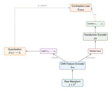
The representations learned by wav2vec 2.0 are remarkably effective for speech retrieval. By extracting frame-level embeddings from the transformer layers and pooling them (via mean pooling or attention-based aggregation), one obtains utterance-level representations that capture both acoustic and linguistic content. These representations can then be indexed and searched using the approximate nearest-neighbour techniques developed in earlier sections of this chapter.
HuBERT: masked prediction of pseudo-labels.
While wav2vec 2.0 uses a contrastive objective with learned quantisation targets, HuBERT [71] (Hidden-Unit BERT) takes a different approach: it performs masked prediction against offline-discovered pseudo-labels. The training proceeds in iterations:
Cluster: Apply -means clustering to MFCC features (first iteration) or to representations from the previous model (subsequent iterations) to produce frame-level pseudo-labels .
Predict: Train a transformer model to predict the pseudo-label at masked positions from the unmasked context, using a cross-entropy loss: (Hubert LOSS) where is the set of masked positions and denotes the unmasked input.
Iterate: Use the trained model's representations to generate better pseudo-labels for the next iteration.
The iterative refinement is key: initial pseudo-labels from MFCC clustering are crude, capturing only basic acoustic properties. But as the model improves, its representations yield increasingly linguistically meaningful clusters, which in turn provide better training targets. This bootstrapping process converges to representations that rival or exceed those of wav2vec 2.0 on downstream tasks.
WavLM: speech processing across the full stack.
WavLM [72] builds on HuBERT's masked prediction framework but adds denoising objectives that make the learned representations robust to noise, reverberation, and overlapping speakers. During training, the input audio is augmented by mixing with noise and other utterances, while the prediction targets remain the clean pseudo-labels. This forces the model to learn representations that are invariant to acoustic degradation, a critical property for retrieval in real-world conditions where recordings are rarely studio-quality.
WavLM additionally benefits from a gated relative position bias in its transformer architecture, which provides more flexible modelling of temporal dependencies than absolute position embeddings.
Theorem 5 (Denoising Objective as Contrastive Learning).
Let denote a corrupted version of audio , obtained by mixing with noise at signal-to-noise ratio : where . Let denote the pseudo-label for frame derived from the clean signal. The WavLM denoising objective implicitly learns a representation such that for any noise realisation , where as . In other words, the denoising objective produces representations that are Lipschitz continuous with respect to additive noise, with the Lipschitz constant decreasing as the noise level decreases.
This noise robustness is critical for speech retrieval in real-world settings: meeting recordings contain air conditioning hum, keyboard clicks, and cross-talk; field recordings suffer from wind noise and equipment handling; phone calls are degraded by codec compression and network jitter. Models trained with denoising objectives produce stable embeddings under all these conditions, enabling retrieval systems that work reliably outside the laboratory.
| Model | Parameters | Pre-training Data | Objective | Key Innovation |
| wav2vec 2.0 | 317M | 960h (LS) / 60kh (LV) | Contrastive | Learned quantisation |
| HuBERT | 316M | 960h (LS) / 60kh (LV) | Masked prediction | Iterative pseudo-labels |
| WavLM | 316M | 960h (LS) / 94kh (mix) | Masked prediction | Denoising augmentation |
Whisper: Universal ASR via Weak Supervision
A fundamentally different approach to speech retrieval is to transcribe the speech into text and then apply standard text retrieval techniques. The viability of this approach depends entirely on the quality of the automatic speech recognition (ASR) system. For decades, ASR errors propagated catastrophically into the retrieval pipeline, degrading recall by 20–40% relative to retrieval on manual transcriptions. Whisper [73] changed this calculus.
Whisper is a sequence-to-sequence transformer trained on 680,000 hours of weakly supervised audio-transcript pairs collected from the internet. The key insight is scale over curation: rather than training on a small, carefully transcribed dataset, Whisper trains on a massive, noisy dataset and relies on the model's capacity to learn robust transcription despite label noise.
The architecture follows a standard encoder-decoder transformer. The audio encoder processes log-mel spectrograms (80 channels, computed from 25,ms windows with a 10,ms stride) through a stack of transformer blocks with sinusoidal position embeddings. The text decoder autoregressively generates tokens conditioned on the encoder outputs and previously generated tokens. Special tokens control language identification, timestamp prediction, and translation.
The scale of Whisper's training is worth emphasising. The 680,000 hours of audio span 99 languages, collected by filtering internet audio-transcript pairs for quality using heuristic alignment checks. The largest model configuration (Whisper Large V3) uses 1.55 billion parameters with a 32-layer encoder and 32-layer decoder, each with 1,280-dimensional hidden states and 20 attention heads. Training was performed on a cluster of GPUs for multiple weeks, a brute-force investment in scale that, combined with the massive and diverse dataset, produced a model with remarkable robustness to accents, background noise, and domain shifts. For retrieval purposes, this robustness translates directly to transcript quality: fewer ASR errors mean less information loss in the transcribe-then-retrieve pipeline.
Definition 31 (Whisper Transcription for Retrieval).
Given a speech archive and a text query , the Whisper-based retrieval pipeline operates in two phases:
Offline indexing: For each audio document , compute transcript and index using a standard text retrieval system (BM25, dense retrieval, etc.).
Online query: Retrieve documents by matching query against the transcript index:
When the query is itself spoken, an additional ASR step transcribes the query: .
The effectiveness of Whisper-based retrieval stems from the model's remarkable robustness. Whisper achieves near-human word error rates across a wide range of accents, noise conditions, and domains, making the transcribe-then-retrieve pipeline competitive with (and often superior to) direct acoustic retrieval for languages where Whisper performs well.
Remark 25.
The transcribe-then-retrieve approach has a fundamental limitation: it discards all paralinguistic information. A query like “find the meeting where someone sounded angry about the budget” cannot be answered from transcripts alone. This limitation motivates hybrid approaches that combine ASR transcripts with acoustic embeddings, preserving both lexical and paralinguistic content in the index.
Spoken Document Retrieval: Architectures Compared
With all these components in hand, we can now compare the two main architectural paradigms for spoken document retrieval.
The ASR-based pipeline transcribes audio into text and applies text retrieval. Its strengths are modularity (any ASR system can be combined with any text retrieval system), interpretability (users can see the transcripts and understand why a document was retrieved), and the ability to leverage decades of progress in text retrieval. Its weakness is error propagation: ASR errors, particularly on named entities, technical terms, and code-switched speech, directly degrade retrieval performance.
The embedding-based pipeline maps both audio and queries directly into a shared embedding space, bypassing transcription entirely. Self-supervised models like wav2vec 2.0, HuBERT, or WavLM produce fixed-dimensional embeddings that capture acoustic and linguistic content. Retrieval is performed by nearest-neighbour search in embedding space. This approach is robust to ASR errors (there is no ASR step to produce errors), works for any language (no language-specific training required), and preserves paralinguistic information. Its weakness is the loss of fine-grained lexical information: embedding-based retrieval may miss exact keyword matches that BM25 would catch.
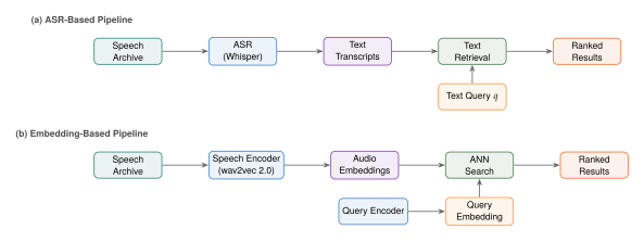
In practice, the best systems often combine both paradigms. A hybrid retrieval system might use BM25 on Whisper transcripts for initial candidate generation (leveraging exact keyword matching), then re-rank using embedding similarity from a self-supervised speech model (incorporating acoustic and semantic information). This two-stage architecture captures the strengths of both approaches while mitigating their individual weaknesses.
Historical Note.
The TREC Spoken Document Retrieval (SDR) track, held from 1997 to 2000, was the first systematic evaluation of spoken document retrieval systems. The task was to retrieve relevant segments from a corpus of broadcast news recordings in response to text queries. The surprising finding was that even with 1990s-era ASR systems producing word error rates of 25–35%, retrieval performance degraded only modestly compared to retrieval on perfect transcripts. This robustness was attributed to the redundancy of natural language: even when ASR corrupts some words, enough correct terms survive to support effective retrieval via TF-IDF matching. The TREC SDR results shaped the field's trajectory for two decades, establishing the transcribe-then-retrieve paradigm as the dominant approach and demonstrating that speech retrieval was “essentially a solved problem” for broadcast news. It took the demands of more challenging domains, including conversational speech, low-resource languages, and multi-speaker meetings, to reveal the limitations of this paradigm and motivate the embedding-based approaches that now complement it.
Example 18 (Hybrid Speech Retrieval System).
Consider a corporate meeting archive containing 50,000 hours of recordings. A hybrid retrieval system operates as follows:
Offline processing: itemize
Transcribe all meetings using Whisper (large-v3), producing timestamped transcripts.
Segment transcripts into passages of approximately 200 words, respecting speaker turn boundaries.
Index passages with BM25 and compute dense embeddings using a WavLM-based utterance encoder. itemize
Online retrieval: Given query : itemize
Retrieve top-100 passages by BM25 score on transcripts.
Retrieve top-100 passages by cosine similarity of WavLM embeddings.
Merge candidate sets and re-rank using a cross-encoder that attends to both transcript text and audio features. itemize
Output: Return ranked list of meeting segments with timestamps, speaker labels, and transcript excerpts.
The hybrid system recovers from ASR errors on technical jargon (caught by the embedding retriever) while maintaining precision on named entities (caught by the text retriever).
Proposition 17 (Error Propagation in ASR-Based Retrieval).
Let denote the word error rate of the ASR system, and assume errors are uniformly distributed across word positions. For a BM25-style retrieval function where the score depends on the presence of query terms in the document, the expected recall loss from ASR errors is bounded by (ASR Recall LOSS) where is the number of query terms. For a query with terms and , the expected recall is at least of the perfect-transcript recall. This exponential degradation in query length explains why ASR-based retrieval is particularly vulnerable on long, specific queries, while short queries with common terms remain robust.
Exercise 30 (DTW Complexity Analysis).
Consider a query-by-example spoken term detection system operating on an archive of hours of audio, with features extracted at a rate of frames per second.
If the query has duration seconds, what is the total number of DTW cells evaluated in a brute-force search (without band constraint)?
Derive the speedup factor from applying a Sakoe–Chiba band of width (10% of the query length).
If each DTW cell evaluation takes floating-point operations (for -dimensional features), and the hardware can perform FLOPS, how long would the brute-force search take for hours, , second, and (standard MFCC dimensionality)?
Propose a two-stage approach that reduces search time by orders of magnitude while maintaining high recall.
Exercise 31 (Self-Supervised Representations for Retrieval).
Suppose you are building a spoken document retrieval system for a low-resource language with only 10 hours of transcribed data but 100,000 hours of untranscribed recordings.
Explain why the ASR-based pipeline is unlikely to work well in this setting.
Describe how you would use wav2vec 2.0 or HuBERT representations for embedding-based retrieval.
The self-supervised model was pre-trained on English. Discuss the transfer learning challenges for a typologically different language (e.g., a tonal language like Mandarin or a polysynthetic language like Inuktitut).
Propose a fine-tuning strategy that uses the 10 hours of labelled data to improve retrieval performance beyond the zero-shot baseline.
Music Information Retrieval
You are in a coffee shop when a song begins playing through the speakers, something you have heard before but cannot quite place. You pull out your phone, open an app, hold it up for a few seconds, and within moments the screen displays the song title, artist, and album art. This act, so casual that it barely registers as remarkable, depends on one of the most elegant algorithms in all of computer science: audio fingerprinting. More broadly, it exemplifies the field of Music Information Retrieval (MIR), which encompasses the computational analysis of, search through, and recommendation of music.
This section explores three facets of music retrieval: exact identification (“What song is this?”), similarity-based search (“Find songs that sound like this one”), and the modern integration of music with language models.
Audio Fingerprinting: The Shazam Algorithm
The Shazam algorithm, published by Wang [74], solves a needle-in-a-haystack problem: given a short, noisy recording captured through a phone's microphone in a crowded environment, identify the exact song from a database of millions of tracks. The solution is based on three key ideas: spectral peak extraction, combinatorial hashing, and hash-table lookup.
Definition 32 (Audio Fingerprint).
Given an audio signal , an audio fingerprint is a compact, content-based signature satisfying three properties:
Discriminability: Different songs produce different fingerprints with high probability: for a small error tolerance .
Robustness: The fingerprint is invariant to common distortions (background noise, reverberation, dynamic range compression, minor pitch shifts): .
Compactness: Each hash is a fixed-length bit string (typically 32 bits), enabling efficient storage and lookup in a hash table.
The Shazam algorithm constructs fingerprints through a process that is best understood as building a constellation map of the audio signal's time-frequency structure.
Step 1: Spectrogram computation.
Compute the short-time Fourier transform (STFT) of the audio signal, producing a spectrogram , where is the STFT coefficient at time frame and frequency bin .
Step 2: Peak extraction.
Identify spectral peaks: time-frequency points where the spectrogram energy is a local maximum, exceeding the energy of all neighbouring points within a region of size . These peaks are remarkably robust to noise and distortion because they correspond to the dominant resonances in the audio signal, which persist even when the signal is degraded.
Step 3: Constellation map.
The set of all spectral peaks forms the constellation map. This map is a sparse representation of the audio signal that discards most of the spectrogram energy and retains only the structural skeleton.
Step 4: Combinatorial hashing.
For each anchor point in the constellation map, select nearby points within a target zone and form a hash: (Shazam HASH) The hash encodes the frequencies of the anchor and target peaks and their time difference. Each hash is stored in a hash table along with the song identifier and the anchor time :
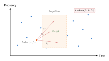
Step 5: Matching and verification.
Given a query recording, the same process is applied to extract query hashes . Each query hash is looked up in the hash table to retrieve candidate matches. A true match produces a coherent time offset: if the query was captured starting at time in the original song, then all matching hashes should satisfy . The song with the most coherent matches (the largest peak in the histogram of time offsets) is returned as the identification.
Algorithm 7 (Audio Fingerprint Matching).
- Input: Query audio ; hash table mapping hashes to pairs; minimum match count
- Output: Identified song or (no match)
- Compute spectrogram
- Extract peaks:
- Generate hashes: Anchor-target pairs
- Initialise offset histograms:
- for each
- for each
- Time offset
- if
- return
- else
- return No confident match
The elegance of Algorithm 7 lies in its hash-table lookups: for each query hash, the lookup returns a small set of candidate matches, and the time-offset histogram aggregates evidence across all query hashes to identify the correct song. The entire process typically completes in under one second for a database of millions of songs.
Remark 26.
The hash function in (Shazam HASH) encodes three quantities: two frequencies and a time difference. The frequencies provide spectral discrimination (different instruments and notes produce peaks at different frequencies), while the time difference provides temporal discrimination (different rhythmic patterns produce different inter-peak timings). The choice to use pairs of peaks rather than individual peaks is critical: a single peak at frequency is far too common to be discriminative (thousands of songs may have energy at 440,Hz), but a pair of peaks at frequencies and separated by time is far more specific. This combinatorial structure is what makes the fingerprint both robust (peaks survive noise) and discriminative (peak pairs are rare enough to identify specific songs).
Proposition 18 (Fingerprint Collision Probability Bound).
Let each hash encode two frequency values quantised to bins and one time difference quantised to bins, so the hash space has size . For a query with hashes and a database song with hashes, assuming hashes are uniformly distributed, the expected number of spurious hash collisions is (Collision Bound) For typical values , , , and , this gives , far below the threshold required for a match. The probability that a non-matching song produces or more coherent collisions is bounded by (Collision TAIL) where is the match threshold and is the number of distinct time-offset bins.
Proof.
Each pair of hashes (one from the query, one from the database song) collides with probability under the uniformity assumption, since both hashes are drawn independently from the same hash space. By linearity of expectation, the expected number of collisions across all pairs is .
For a false match, or more of these collisions must additionally agree on the same time offset, which occurs with probability per collision. A union bound over all subsets of collisions gives the stated tail bound.
Music Similarity and Recommendation
While fingerprinting answers “What song is this?”, a different question drives much of music information retrieval [75][76]: “What songs sound like this one?” Answering this question requires extracting features that capture the perceptual qualities of music and defining meaningful similarity measures over these features.
Music features are traditionally organised into a hierarchy spanning three levels of abstraction.
Definition 33 (Music Feature Hierarchy).
Low-level features capture the acoustic surface of the signal: itemize
Spectral centroid: the “centre of mass” of the spectrum, correlating with perceived brightness.
Spectral flux: frame-to-frame spectral change, correlating with perceived “activity”.
Mel-frequency cepstral coefficients (MFCCs): compact representations of the spectral envelope, widely used for timbral similarity.
Zero-crossing rate: correlates with noisiness and percussive content. itemize
Mid-level features capture musical structure: itemize
Tempo and beat strength: rhythmic properties estimated via onset detection and autocorrelation.
Chroma features: the distribution of spectral energy across the twelve pitch classes, capturing harmonic content independent of octave.
Onset patterns: the rhythmic pattern of note onsets, capturing groove and rhythmic complexity. itemize
High-level features capture semantic and cultural properties: itemize
Genre: classification into categories (rock, jazz, classical, etc.).
Mood: emotional characterisation (happy, sad, energetic, calm).
Instrumentation: presence and prominence of specific instruments. itemize
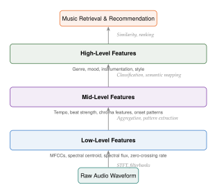
Music similarity is then computed by representing each song as a feature vector (or sequence of feature vectors) and measuring distance in feature space. A common approach represents a song by the mean and covariance of its frame-level MFCC vectors [77], forming a Gaussian model per song, and measures similarity using the Kullback–Leibler divergence between these Gaussians: (Music Similarity KL) where and are the mean and covariance of the MFCC distributions for songs and respectively, and is the feature dimensionality.
Query-by-Humming
One of the most user-friendly forms of music retrieval is query-by-humming (QBH): a user hums, sings, or whistles a melody, and the system identifies the song. This is a fundamentally different problem from fingerprinting because the query is a highly distorted version of the original: the rhythm may be approximate, the pitch may be shifted, and the timbre is entirely different (a human voice rather than instruments).
The QBH problem reduces to melody matching: comparing the pitch contour of the hummed query against a database of reference melodies. The pitch contour is extracted from the query using a fundamental frequency () estimation algorithm, producing a sequence of pitch values . Reference melodies can be extracted from MIDI files, audio recordings, or music score databases.
Matching is performed using a variant of DTW that operates on pitch intervals (differences between consecutive pitch values) rather than absolute pitch values, making the system transposition-invariant: (QBH DTW) where and are the query and reference pitch sequences respectively. This formulation ensures that a query hummed in a different key still matches the correct song.
Insight.
Query-by-humming elegantly illustrates the tension between invariance and discriminability that pervades all of retrieval. The system must be invariant to transposition (key changes), tempo variations (the user may hum faster or slower than the original), timbre differences (voice vs. instruments), and rhythmic imprecision. Yet it must remain discriminative enough to distinguish between melodies that share similar contours. The solution, operating on pitch intervals with DTW alignment, achieves the right balance by preserving the melodic shape while discarding absolute pitch and timing.
Modern Approaches: Neural Music Representations
The feature engineering approach to music similarity is being supplanted by deep learning models that learn representations end-to-end. Two recent models illustrate this trend.
MusicGen.
MusicGen [78] is a language model for music generation that operates on discrete audio tokens produced by EnCodec, a neural audio codec. While designed for generation, MusicGen's internal representations (the hidden states of its transformer layers) serve as powerful feature extractors for music retrieval. These representations encode harmonic, rhythmic, and timbral information at multiple levels of abstraction, learned implicitly through the generation objective.
MusicLM.
MusicLM [79] generates high-fidelity music from text descriptions by combining MuLan (a music-text embedding model) with AudioLM (an audio language model). The MuLan embedding space, where music and text descriptions are aligned, provides a natural basis for text-to-music retrieval: given a text query like “upbeat jazz piano with brushed drums,” retrieve songs whose MuLan embeddings are closest to the text embedding.
These models represent a paradigm shift: instead of hand-engineering features for each aspect of music (timbre, rhythm, harmony), a single model learns a unified representation that captures all relevant dimensions simultaneously. For retrieval, this means that a single embedding can support diverse query types, from acoustic similarity to semantic text-based search.
Example 19 (Neural Music Feature Extraction).
To use MusicGen as a feature extractor for music retrieval, one processes each song through the model's encoder and extracts hidden-state representations at multiple layers:
Encode the audio using EnCodec to produce discrete tokens .
Pass the tokens through MusicGen's transformer layers, extracting hidden states at layer for each position .
Aggregate across positions via mean pooling: .
Concatenate representations from multiple layers to capture both low-level acoustic details (early layers) and high-level semantic properties (late layers): .
The resulting representation can be used for nearest-neighbour retrieval, clustering, or as input to a downstream recommendation model. Empirically, mid-to-late layers (e.g., layers 8–12 in a 24-layer model) produce the best retrieval features, capturing musical structure without being overly specialised for the generation objective.
Remark 27.
The use of generative models as feature extractors is a recurring theme in modern retrieval. Just as large language models pre-trained for text generation produce excellent text embeddings, and diffusion models pre-trained for image generation produce excellent visual features, music generation models produce representations that capture the structure of music far better than hand-crafted features. The generative pre-training objective forces the model to build internal representations of the data distribution, and these representations are precisely what retrieval needs.
Music-Text Retrieval
The connection between music and natural language has become a central focus of modern MIR. Music-text retrieval enables two complementary tasks: text-to-music retrieval (finding songs that match a text description) and music-to-text retrieval (generating or retrieving text descriptions for a given song, often called music captioning).
The dominant approach follows the contrastive dual-encoder paradigm familiar from CLIP and its variants: a music encoder and a text encoder are trained jointly to produce aligned embeddings, using a contrastive loss that pushes matching music-text pairs together and non-matching pairs apart. The CLAP framework [22], discussed in detail in the next section, provides the foundation for this approach.
Content-based vs. collaborative filtering.
Music recommendation systems traditionally use one of two approaches. Content-based filtering recommends songs based on acoustic similarity to songs the user has enjoyed, using the features and similarity measures described above. Collaborative filtering recommends songs based on the listening patterns of similar users, without analysing the audio content at all. Modern systems combine both approaches in hybrid recommenders that use content-based features to address the cold-start problem (recommending new songs with no listening history) while leveraging collaborative signals for personalisation.
The emergence of music-text models adds a third dimension: users can now describe what they want in natural language, and the system can retrieve music that matches the description even if the user has never heard similar music before. This language-mediated retrieval is particularly powerful because natural language can express complex, compositional musical concepts (“a slow, melancholic cello piece reminiscent of Elgar”) that are difficult to capture with acoustic features alone.
Proposition 19 (Cold-Start Advantage of Content-Based Retrieval).
Let be a set of users, a set of songs, and the binary interaction matrix. A new song added to the catalogue has for all (no user has interacted with it). Collaborative filtering methods, which predict ratings from the interaction matrix alone, assign zero or uniform scores to for all users, rendering them unable to recommend it. In contrast, content-based methods can compute similarity for all existing songs using acoustic features, enabling immediate recommendation to users who enjoyed acoustically similar songs. The collaborative filtering model requires at least interactions with before its latent factor estimate achieves bounded error, while content-based similarity requires zero interactions.
Example 20 (Music Information Retrieval Pipeline).
A modern music streaming platform integrates multiple retrieval modalities:
Exact identification: Shazam-style fingerprinting for “What's playing?” queries. Hash-table lookup over a database of 100 million tracks, completing in under 1 second.
Acoustic similarity: Neural embeddings (from MusicGen or a dedicated music embedding model) enable “More like this” recommendations. Approximate nearest-neighbour search in a learned embedding space.
Text-based search: CLAP embeddings enable natural language queries (“chill lo-fi beats for studying”). The music encoder and text encoder produce embeddings in a shared space, and cosine similarity ranks the results.
Collaborative filtering: User listening histories provide personalised recommendations via matrix factorisation or graph neural network models.
Hybrid fusion: A learned re-ranker combines signals from all modalities, weighting acoustic, semantic, and collaborative evidence to produce the final ranking.
Exercise 32 (Audio Fingerprint Design).
Consider designing an audio fingerprinting system for a database of songs, each of average duration 4 minutes, with audio sampled at 44.1,kHz.
If the STFT uses a window of 1,024 samples with 75% overlap, how many time frames are produced per song? If the peak density is 5 peaks per time frame, how many peaks are in the full database?
If each anchor point is paired with 10 target points, how many hashes are produced per song? What is the total hash-table size for the full database?
Using the collision bound from Proposition 18, compute the expected number of spurious collisions for a 5-second query against each non-matching song. What match threshold ensures a false-positive rate below per song?
Describe how you would modify the fingerprinting algorithm to handle time-stretched audio (e.g., a DJ playing a song at 105% of normal speed).
Exercise 33 (Query-by-Humming System Design).
A query-by-humming system receives a hummed melody and must identify the song from a database of 1 million tracks.
The estimator produces a pitch sequence at 100,Hz frame rate with occasional octave errors (the estimated pitch is exactly twice or half the true pitch). Design a preprocessing step that detects and corrects octave errors using the smoothness of the pitch contour.
The interval-based DTW in (QBH DTW) is transposition-invariant but not tempo-invariant. Propose a two-stage approach that first normalises the query to a canonical tempo and then applies DTW.
Discuss the limitations of melody-based retrieval for genres where the melody is not the primary distinguishing feature (e.g., electronic dance music, ambient music). What alternative query modalities might be effective?
Exercise 34 (Music Similarity Metrics).
Given a database of songs represented by Gaussian MFCC models :
Prove that the KL divergence between two Gaussians is not symmetric. Define a symmetric version and discuss its properties as a similarity metric.
The KL divergence has computational cost due to the matrix inverse and determinant. Propose a diagonal covariance approximation and analyse the resulting complexity.
A user wants to find songs that are “rhythmically similar but timbrally different.” How would you modify the feature representation and similarity metric to support this query?
Audio-Language Retrieval
The previous two sections focused on speech and music, two structured forms of audio with well-developed retrieval traditions. But the auditory world extends far beyond speech and music: the creak of a door, the rumble of thunder, a car horn in traffic, the chirping of crickets at dusk. General audio retrieval, the ability to search for arbitrary sounds using natural language descriptions, has emerged as a frontier where audio understanding meets language understanding, producing models that can find sounds they have never been explicitly trained to recognise.
The key enabler is Contrastive Language-Audio Pre-training (CLAP) [22], which extends the CLIP paradigm from images to audio, learning a shared embedding space where audio recordings and text descriptions are aligned.
CLAP: Contrastive Language-Audio Pre-training
CLAP follows the dual-encoder contrastive framework that has proven so effective for vision-language models, adapted for the audio domain. The architecture consists of two components.
Audio encoder.
The audio encoder takes a log-mel spectrogram as input and produces a -dimensional embedding. Common choices include:
HTSAT (Hierarchical Token-Semantic Audio Transformer): a Swin Transformer adapted for audio spectrograms, which captures both local spectral patterns and global temporal structure.
PANN (Pre-trained Audio Neural Network): CNN-based architectures pre-trained on AudioSet for audio tagging, fine-tuned within the CLAP framework.
BEATs: an audio pre-training framework using iterative audio tokenisation and masked prediction.
Text encoder.
The text encoder maps
a text description to the same -dimensional space. CLAP
typically uses a pre-trained language model (RoBERTa, BERT, or
GPT-2) as the backbone, with a projection head that maps the
[CLS] token representation to the shared embedding space.
Training objective.
The model is trained with the symmetric contrastive loss familiar from CLIP: (CLAP LOSS) where is a batch of audio-text pairs, denotes the inner product in the shared embedding space, and is a learnable temperature parameter.
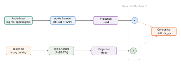
Training data.
CLAP models are trained on audio-text pairs drawn from several sources:
AudioSet [13]: over 2 million 10-second YouTube clips with human-annotated labels, which can be converted to text descriptions via templates (e.g., label “Dog bark” becomes “The sound of a dog barking”).
AudioCaps: a subset of AudioSet with human-written free-form captions describing the audio content in natural language.
LAION-Audio-630K [14]: a large-scale dataset of 633,526 audio-text pairs collected from the web, covering music, environmental sounds, and speech.
FreeSound: a collaborative database of Creative Commons–licensed sounds with user-provided descriptions.
Key Idea.
Zero-shot audio classification as retrieval.
One of CLAP's most powerful capabilities is zero-shot audio
classification. Given an audio clip and a set of candidate class
labels , each label is converted to a text
prompt (e.g., “the sound of [class]”), embedded by the
text encoder, and compared to the audio embedding. The predicted
class is
This is precisely a retrieval operation: the audio “queries” the
text space to find the best-matching description. Remarkably, CLAP
can classify sounds from categories never seen during training,
because the text encoder provides a semantic bridge between seen
and unseen categories through the structure of natural language.
LAION-Audio: Scaling Audio-Text Pre-training
The effectiveness of contrastive audio-language models scales with the size and diversity of the training data. LAION-Audio [14] addresses this by providing a large-scale, openly available dataset of audio-text pairs harvested from the web. The collection pipeline mirrors the approach used for LAION-5B in the image domain:
Crawl web pages containing audio content (YouTube, FreeSound, BBC Sound Effects, etc.).
Extract audio files and their associated text metadata (titles, descriptions, tags, captions).
Filter for quality: remove very short clips (,s), very long clips (,s), and clips with uninformative descriptions.
De-duplicate by audio fingerprinting to avoid training on near-identical clips.
The resulting LAION-Audio-630K dataset contains 633,526 audio-text pairs spanning diverse categories: environmental sounds (rain, traffic, machinery), music (instruments, genres, moods), speech-related sounds (laughter, applause, crowd noise), and animal vocalisations. Models trained on LAION-Audio consistently outperform those trained on AudioSet alone, particularly on out-of-domain retrieval tasks, because the web-sourced data provides greater diversity in both audio content and text descriptions.
Remark 28.
The scaling behaviour of audio-language models follows patterns familiar from vision-language pre-training. Doubling the training data size typically yields a consistent improvement in retrieval recall, with diminishing returns setting in only at very large scales. However, the quality of audio-text alignment matters as much as quantity: a smaller dataset of human-written captions (like AudioCaps) can produce better retrieval performance per training example than a larger dataset of template-generated descriptions from class labels. The ideal training mixture combines both: template-expanded label data provides broad coverage across sound categories, while human captions provide the linguistic diversity and compositionality needed for free-form text queries.
ImageBind: Binding Audio to Other Modalities
CLAP binds audio to text. CLIP binds images to text. A natural question arises: can we bind all modalities, including audio, images, text, video, depth, and thermal, into a single shared embedding space? ImageBind [15] provides an affirmative answer through a remarkably elegant mechanism.
The key insight is that images can serve as a universal binding modality. Because high-quality paired data exists between images and each other modality (image-text pairs, image-audio pairs from video, image-depth pairs from RGB-D sensors), training separate encoders to align each modality with images implicitly aligns all modalities with each other. If audio embedding is close to image embedding in one space, and text embedding is close to image embedding in another space, then and should be close to each other, even though they were never directly paired during training.
Theorem 6 (Emergent Cross-Modal Alignment).
Let be encoders for modalities, and let be the image encoder serving as the binding modality. Suppose each encoder is trained to minimise the contrastive loss against the image encoder. If the learned embedding space is approximately isometric (distances are approximately preserved under the encoder mappings), then for any two modalities , the cross-modal retrieval performance is bounded below by (Imagebind Bound) where captures the deviation from perfect isometry and denotes retrieval recall.
Proof sketch.
Consider a query from modality and a database in modality . The true match is the item whose underlying semantic content matches the query. In the shared embedding space, the query embedding is close to the image embedding of the corresponding image (by the alignment between and images), and the database item embedding is close to (by the alignment between and images). By the triangle inequality in the embedding space: When both terms on the right are small (which happens when both modality-to-image alignments are good), the cross-modal distance is also small, ensuring that the correct match is retrieved. The deviation accounts for cases where the triangle inequality bound is not tight.
The practical implication is striking: by training modality-specific encoders against a single image encoder, ImageBind obtains pairwise retrieval capabilities, of which only are directly trained. For modalities, this means 15 pairwise tasks from only 5 trained alignments, a 3 amplification of retrieval capabilities.
For audio retrieval, ImageBind's contribution is the ability to perform cross-modal audio retrieval without direct audio-text or audio-image paired training data. Given a text query, one can retrieve audio clips by comparing text embeddings to audio embeddings in the shared space, even if the model was trained only on image-text and image-audio pairs. This emergent capability dramatically expands the scope of audio retrieval.
Example 21 (Cross-Modal Retrieval via ImageBind).
Consider a database of environmental audio recordings indexed using ImageBind's audio encoder. The following cross-modal queries become possible:
Text-to-audio: “crashing ocean waves” retrieves recordings of surf and breaking waves.
Image-to-audio: A photograph of a thunderstorm retrieves recordings of thunder and rain.
Audio-to-image: A recording of birdsong retrieves images of forests and birds.
Video-to-audio: A silent video of a waterfall retrieves the sound of rushing water.
All four query types are supported by a single model, despite the model never being trained on direct audio-text, audio-image, or audio-video pairs. The binding through the image modality creates these emergent retrieval capabilities.
Sound Event Retrieval
Sound event retrieval focuses on finding specific sounds within audio recordings based on textual descriptions. This capability is essential for applications including sound effect production (finding the right door creak for a film), environmental monitoring (detecting specific bird calls in ecological surveys), and accessibility (alerting hearing-impaired users to relevant environmental sounds).
The retrieval task can be formalised as follows.
Definition 34 (Sound Event Retrieval).
Given a text query describing a sound event (e.g., “a glass bottle breaking on a tile floor”) and a database of audio clips , retrieve the set of clips that contain the described event: where and are the text and audio encoders of a CLAP model and is a relevance threshold.
The challenge in sound event retrieval lies in the compositionality of natural language descriptions. A query like “a dog barking in the distance with traffic noise in the background” requires the model to understand multiple concurrent sound sources, their spatial relationships, and their relative prominence. Current CLAP models handle simple compositional queries reasonably well but struggle with complex spatial or temporal relationships.
Environmental sound classification provides an important testing ground for audio retrieval models. The ESC-50 benchmark, containing 2,000 five-second recordings across 50 classes of environmental sounds (from “dog bark” to “chainsaw” to “pouring water”), has become the standard evaluation for zero-shot audio understanding. A CLAP model achieves zero-shot classification on ESC-50 by computing the similarity between the audio embedding and text embeddings for each of the 50 class labels, selecting the label with the highest similarity. The progression from 72% accuracy (early CLAP models) to over 93% (current state of the art) reflects improvements in both model architecture and training data scale.
Lemma 5 (Retrieval as Classification).
Let and be a CLAP model's audio and text encoders, and let be a set of class labels with text prompts . The zero-shot classification decision is equivalent to a 1-nearest-neighbour retrieval in the text embedding space, where the “database” consists of the class embeddings and the “query” is the audio embedding. If the text embeddings are approximately uniformly distributed on the unit sphere (a consequence of the contrastive training objective for large ), then the classification boundary between classes and is the hyperplane , yielding a Voronoi tessellation of the embedding space.
| Model | AudioCaps | Clotho | ESC-50 (ZS) | Training Data |
| CLAP (HTSAT) | 57.8 | 27.4 | 82.6 | AudioSet + AudioCaps |
| LAION-CLAP | 64.2 | 33.1 | 90.4 | LAION-Audio-630K |
| ImageBind | 51.3 | 22.8 | 77.2 | Image-paired data |
| MS-CLAP (2023) | 68.7 | 36.2 | 93.1 | AudioSet + LAION + FSD50K |
Retrieval-Augmented Audio Generation
A natural application of audio retrieval is to enhance audio generation models by grounding them in retrieved examples. Just as retrieval-augmented generation (RAG) improves text generation by conditioning on relevant documents, retrieval-augmented audio generation improves the fidelity and controllability of audio synthesis by conditioning on retrieved audio clips.
Re-AudioLDM.
Re-AudioLDM [32] augments the AudioLDM [80] latent diffusion model with a retrieval module. Given a text prompt describing the desired audio (e.g., “rain falling on a metal roof with occasional thunder”), the system first retrieves the most relevant audio clips from a database using CLAP embeddings, then conditions the diffusion process on both the text prompt and the retrieved audio features: (Reaudioldm) where is the text conditioning, is the set of retrieved audio clips, and denotes the reverse diffusion process. The retrieved clips provide concrete acoustic examples that guide the diffusion process toward generating audio with the right timbral and spectral characteristics.
RECAP.
RECAP [33] takes a complementary approach, focusing on the retrieval of audio captions rather than audio clips. Given a text prompt, RECAP retrieves similar captions from a large database and uses them to enrich the text conditioning for the generation model. This is particularly effective for underspecified prompts: a user who writes “ocean” gets the benefit of retrieved captions like “gentle waves lapping on a sandy beach with distant seagulls,” which provide the acoustic detail needed for high-quality generation.
Definition 35 (Retrieval-Augmented Audio Generation).
A retrieval-augmented audio generation system consists of three components:
A retrieval module that maps a text query to a set of relevant audio clips or captions from a database.
A conditioning mechanism that fuses the text prompt with the retrieved items to produce a conditioning vector.
A generation model that produces audio conditioned on the fused representation.
The generation quality is bounded below by the retrieval quality: if the retrieved items are relevant and diverse, the conditioning provides rich acoustic detail; if the retrieval fails, the system falls back to text-only conditioning.
Insight.
Retrieval-augmented audio generation exemplifies a broader principle: retrieval and generation are complementary, not competing, paradigms. Pure generation must synthesise all acoustic details from a text description alone, placing enormous demands on the model's capacity and training data. Retrieval-augmented generation offloads part of this burden to the database: instead of learning to generate every possible sound from scratch, the model learns to adapt and recombine retrieved examples, a fundamentally easier task. This parallels the observation in language modelling that RAG systems can achieve the performance of much larger models by leveraging external knowledge. In the audio domain, the principle is even more powerful: audio signals are high-dimensional and exhibit enormous variability (the sound of “rain” can vary along dimensions of intensity, surface material, accompanying sounds, and recording conditions), making it far easier to retrieve a close example and adapt it than to synthesise the full acoustic detail from a text description alone.
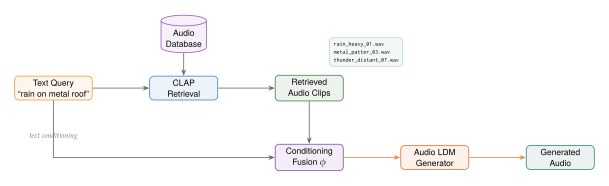
Example 22 (Audio-Language Retrieval in Practice).
Consider a sound designer working on a nature documentary who needs to find specific environmental sounds. Using a CLAP-based retrieval system with a database of 500,000 environmental recordings:
Query: “gentle stream flowing over rocks in a forest” itemize
The text encoder maps this description to an embedding that captures both the acoustic qualities (flowing water, natural setting) and the semantic context (gentle, forest).
The top-5 retrieved clips include brook recordings with varying levels of bird activity and wind. itemize
Query: “footsteps on gravel, slow pace” itemize
The model retrieves recordings of walking on gravel surfaces, ranked by tempo match (slower footsteps ranked higher).
The temporal descriptor “slow pace” is captured through the model's learned association between text and acoustic features. itemize
Query: “thunderstorm approaching from a distance” itemize
Results are ranked by the prominence and spatial characteristics of the thunder, with distant rumbles ranked above close strikes.
This demonstrates the model's ability to understand spatial relationships described in text. itemize
Exercise 35 (CLAP Training Dynamics).
Consider training a CLAP model from scratch on a dataset of audio-text pairs.
In the contrastive loss ((CLAP LOSS)), what happens when the temperature is very small ()? What about when it is very large ()? Discuss the effect on gradient magnitude and learning dynamics.
The contrastive loss treats all non-matching pairs equally. Propose a modification that assigns different negative weights based on semantic similarity of the text descriptions (e.g., “dog barking” and “puppy yelping” should be softer negatives than “dog barking” and “piano playing”).
Derive the gradient of with respect to the audio embedding for the -th example, and show that it pushes the audio embedding toward its matching text and away from non-matching texts, with forces proportional to the softmax-weighted similarities.
How does the batch size affect the quality of the learned representations? Provide both an information-theoretic argument (in terms of the mutual information lower bound) and a practical argument (in terms of the hardness of negatives).
Exercise 36 (Cross-Modal Retrieval Analysis).
ImageBind aligns modalities to a shared embedding space using images as the binding modality.
How many pairwise retrieval tasks are possible with 6 modalities? How many of these are directly trained (i.e., involve the image modality)? What fraction of all retrieval capabilities are emergent?
Using Theorem 6, if audio-to-image recall is and text-to-image recall is , what is the lower bound on audio-to-text recall?
The bound in (Imagebind Bound) can be negative. Under what conditions does this happen, and what does it mean? Propose a tighter bound using concentration inequalities on the embedding distances.
Design an experiment to test whether the triangle inequality assumption underlying ImageBind's emergent alignment holds in practice. What embedding properties would cause the assumption to fail?
Exercise 37 (Retrieval-Augmented Audio Generation).
Consider a retrieval-augmented audio generation system that uses CLAP embeddings to retrieve reference clips and conditions an AudioLDM model on the retrieved features.
Formalise the retrieval step as an optimisation problem. What objective does the CLAP-based retriever optimise, and how does this relate to the generative model's conditioning requirements?
The choice of (number of retrieved clips) involves a bias-variance tradeoff. With , the generation is strongly influenced by a single example; with , the retrieved set may include irrelevant clips that dilute the conditioning signal. Propose a method for adaptively selecting based on the retrieval scores.
When the text prompt is ambiguous (e.g., “bird”), the retrieved clips may span diverse interpretations (songbirds, seagulls, parrots). How would you modify the system to present diverse generation options to the user rather than averaging over interpretations?
Caution.
Audio-language models inherit biases from their training data. Web-sourced audio datasets are heavily skewed toward English descriptions, Western music genres, and urban soundscapes from developed countries. A CLAP model may perform poorly on queries in other languages, fail to recognise traditional instruments from non-Western musical traditions, or misclassify environmental sounds common in rural or tropical settings but rare in the training data. Evaluating and mitigating these biases is an active research challenge that becomes more urgent as these models are deployed in global applications.
Open Problem 2.
Several open problems define the frontier of audio-language retrieval: The field of audio-language retrieval is young, with CLAP models first appearing in 2022, and much remains to be understood about the structure of audio-text embedding spaces, the optimal training strategies, and the limits of what contrastive pre-training can achieve for audio understanding.
Temporal reasoning: Current CLAP models treat audio as a single “bag of events.” Queries that require temporal reasoning (“a car horn followed by screeching tires and then a crash”) are poorly served. Extending CLAP to capture temporal structure without sacrificing retrieval efficiency is an open challenge.
Compositional understanding: Natural language descriptions of audio scenes are compositional (“loud” modifies a specific source, “in the background” specifies spatial positioning), but current models struggle with compositional semantics.
Long-form audio retrieval: Most audio-language models operate on 10-second clips. Scaling to minutes or hours, as required for podcast search, surveillance, or ecological monitoring, requires efficient temporal indexing strategies.
Unified audio models: Current systems use separate models for speech, music, and environmental sound. A truly universal audio retrieval system would handle all three with a single encoder, understanding queries like “find the podcast episode where jazz music plays during the interview about climate change.”
Multimodal Embedding Spaces
Imagine a single coordinate system in which a photograph of a thunderstorm, the sound of rolling thunder, the sentence “dark clouds gathering before a downpour,” a video clip of lightning, and even the thermal signature of a storm front all live as nearby points. Not merely nearby within their own modality, but nearby to each other, so that the sound of thunder sits closer to the image of lightning than to the sound of birdsong, and the sentence sits closer to the photograph than to an unrelated paragraph about tax policy. This is the grand vision of multimodal embedding spaces: a single, shared geometric arena in which every form of human experience, text, vision, audio, touch, motion, can be compared, combined, and retrieved with the same inner product.
The vision is revolutionary because it collapses the tower of modality-specific systems that has dominated machine learning for decades. Instead of separate text search, image search, audio search, and video search engines, each with bespoke architectures, training pipelines, and index structures, one obtains a single embedding model and a single vector index. A query in any modality retrieves results in every modality, with relevance measured by a single score.
The vision is also incredibly challenging. Each modality lives on a fundamentally different data manifold. Text is discrete and sequential; images are dense and spatial; audio is temporal and frequency-structured; video is spatiotemporal; depth maps are geometric. Aligning these manifolds into a shared space requires not just large paired datasets but a principled framework for defining what “alignment” even means when the modalities carry different information at different levels of abstraction.
Key Idea.
The Multimodal Alignment Problem. Given modalities with data spaces , the multimodal alignment problem asks for encoders , one per modality, such that semantically related inputs from different modalities map to nearby points in . Formally, for semantically related pairs with : (Multimodal Alignment) for unrelated , where denotes the inner product after -normalization.
The difficulty scales superlinearly with the number of modalities. For modalities, there are pairwise alignment tasks, but paired data is typically available for only a small subset of these pairs. Collecting audio-depth pairs, or text-thermal pairs, or IMU-video pairs at scale is prohibitively expensive. This data scarcity problem is what makes the naive approach of training separate contrastive models impractical, and it is what motivates the elegant solutions we study next.
ImageBind: Binding Six Modalities Through Images
The key insight behind ImageBind [15] is deceptively simple: images are nature's universal pairing mechanism. Consider the modalities we care about: text, audio, depth, thermal imagery, and inertial measurement unit (IMU) data. In the natural world, images are routinely paired with each of these modalities. Web data provides billions of image-text pairs. Videos provide image-audio pairs (every video frame is paired with its soundtrack). RGB-D cameras provide image-depth pairs. Thermal cameras provide image-thermal pairs. Wearable devices with cameras provide image-IMU pairs.
None of these pairings are exotic or expensive; they arise organically from the way sensors capture the world. The genius of ImageBind is to exploit this star topology of natural pairings, with images at the hub, to bind all six modalities into a single embedding space without ever needing direct pairings between non-image modalities.
Definition 36 (Image-Anchored Multimodal Alignment).
Let be a set of modalities, with modality designated as the anchor modality (images). For each non-anchor modality , assume access to paired data . The image-anchored alignment trains modality-specific encoders by minimizing the InfoNCE loss between each modality and the anchor: (Imagebind LOSS) where is a temperature parameter. The total loss is .
The architecture of ImageBind uses a Vision Transformer (ViT-H) as the image encoder , initialized from a pretrained model. Each non-image modality uses a separate Transformer encoder , with modality-specific tokenization: audio spectrograms are treated as 2D patches (following the Audio Spectrogram Transformer approach), depth and thermal maps are treated as single-channel images, IMU signals are treated as 1D sequences, and text uses the standard tokenizer from CLIP [9].
Remark 29 (Why the Star Topology Works).
The star topology works because of the transitivity of embedding alignment. If audio is aligned with images, and text is aligned with images, then audio and text become implicitly aligned through the shared image space. Formally, if is high and is high for semantically related triplets , then tends to be high as well, even though no audio-text pairs were used during training.
This transitivity is not exact (the triangle inequality in embedding space introduces a gap), but empirically it works remarkably well. ImageBind achieves strong zero-shot audio-text retrieval without having seen a single audio-text pair during training.
The emergent cross-modal retrieval capabilities are perhaps ImageBind's most striking contribution. Consider the following: train the model exclusively on (image, audio), (image, text), (image, depth), (image, thermal), and (image, IMU) pairs. Now, at inference time, compute embeddings for an audio clip and a text description. Despite never having been trained on audio-text correspondence, the model can retrieve the correct text given an audio query, and vice versa. This is zero-shot emergent cross-modal retrieval, and it arises purely from the geometry of the shared embedding space.
Proposition 20 (Emergent Alignment Bound).
Let (image), , and be modality encoders trained with image-anchored alignment. For semantically related inputs with a common semantic referent having image representation , the emergent cross-modal similarity satisfies (Emergent Bound) where all embeddings are -normalized.
Proof.
Write , , , all unit vectors, and let be the geodesic (angular) distances on the unit sphere, so that , , and . Geodesic distance is a metric, so the triangle inequality gives . Since is decreasing on , which is the stated bound (the spherical law of cosines). It is tight when are coplanar and lies on the geodesic arc between and .
The practical implication is that image-anchored alignment makes distant modalities align, but the guarantee is weaker than a naive additive estimate suggests. If each pairwise cosine similarity exceeds , the emergent similarity is only guaranteed to exceed (not the additive ), still positive and useful, but a reminder that transitivity of cosine similarity on the sphere is sublinear.
Example 23 (Emergent Audio-Text Retrieval in ImageBind).
On the ESC-50 environmental sound classification benchmark, ImageBind achieves 66.9% zero-shot accuracy for audio classification using text labels, despite never having been trained on any audio-text pairs. The model “hears” a sound (e.g., a crackling fire), embeds it near the image of a fireplace (via the audio-image alignment), and the fireplace image embedding is near the text “crackling fire” (via the image-text alignment inherited from CLIP). The chain produces a zero-shot audio-text connection that performs competitively with CLAP models trained on millions of audio-text pairs. This is the power of a well-structured embedding geometry: information about cross-modal relationships propagates transitively through the shared space.
Remark 30 (Scaling Laws for Emergent Alignment).
The quality of emergent cross-modal alignment improves with three factors: (a) the quality of the image encoder (a better image backbone produces a more semantically structured hub), (b) the quantity of paired data for each spoke of the star (more image-audio pairs improve audio embeddings), and (c) the embedding dimension (higher dimensions provide more room for modality-specific information to coexist with shared semantics). ImageBind uses with a ViT-H backbone, and ablation studies show that reducing the backbone to ViT-B degrades emergent alignment more than it degrades trained alignment, suggesting that emergent capabilities are more sensitive to model capacity.
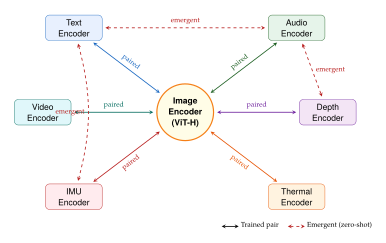
Gemini Embedding 2: Natively Multimodal Embeddings
While ImageBind demonstrated that multimodal alignment could emerge from image-anchored contrastive learning, a natural question followed: what if a model were trained from the ground up to be natively multimodal, understanding text, images, video, audio, and structured documents within a single architecture? Google's Gemini Embedding [16][17] represents exactly this next step, leveraging the full power of the Gemini multimodal foundation model to produce embeddings that are natively multimodal rather than post-hoc aligned.
The key differences from approaches like ImageBind are architectural and philosophical. ImageBind uses separate encoders per modality, aligned through a shared loss. Gemini Embedding uses a single multimodal backbone, the Gemini model itself, which processes all modalities natively through a unified Transformer architecture. The embedding is extracted from this shared representation, yielding a 3072-dimensional vector for any input regardless of modality [18][81].
Definition 37 (Natively Multimodal Embedding).
A natively multimodal embedding model is a function implemented by a single model architecture that processes all modalities through shared parameters, rather than through modality-specific encoders with a shared loss. The embedding dimension is fixed at regardless of input modality.
Matryoshka Representation Learning.
One of the most elegant features of Gemini Embedding is its support for Matryoshka representations. Named after Russian nesting dolls, this technique trains the embedding such that every prefix of the full -dimensional vector is itself a valid, useful embedding at a lower dimension. Formally, let be the full embedding. For any , the truncated embedding (the first coordinates) preserves as much information as possible for that dimensionality.
Definition 38 (Matryoshka Embedding).
A Matryoshka embedding of depth is an embedding trained with the multi-scale loss (Matryoshka LOSS) where are the target dimensionalities, are scale weights, and is the task-specific loss (e.g., InfoNCE for retrieval) evaluated using only the first dimensions of the embedding.
The practical benefit is enormous. A production system can store the full 3072-dimensional embedding for maximum accuracy, but perform initial candidate retrieval using only the first 256 or 512 dimensions for speed and memory efficiency, then re-rank using the full embedding. This yields a natural coarse-to-fine retrieval pipeline without training separate models at each dimensionality.
Task-Type Conditioning.
Gemini Embedding introduces another innovation: task-type
conditioning. Rather than producing a single, task-agnostic
embedding, the model accepts a task_type parameter that
conditions the embedding computation for specific downstream
tasks [17][82]:
retrieval_document: optimized for indexing documents to be retrieved.retrieval_query: optimized for queries that will be matched against documents.semantic_similarity: optimized for computing pairwise similarity between inputs.classification: optimized for downstream classification tasks.clustering: optimized for grouping similar inputs.
Insight.
Asymmetric Query-Document Embeddings.
The separation of retrieval_query and
retrieval_document task types reflects a deep insight
about information retrieval: queries and documents play
fundamentally different roles. A query is short, underspecified,
and expresses an information need. A document is long, detailed,
and contains the information. By conditioning the embedding on
the role of the input, the model can learn to project queries
into the region of embedding space where their relevant documents
reside, rather than forcing a symmetric similarity that treats
both inputs identically. This is the learned analog of the
classical query expansion technique, but implemented within the
embedding computation itself.
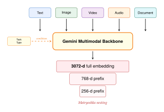
Example 24 (Unified Multimodal Product Search).
Consider an e-commerce platform that needs to support the following queries, all directed at the same product catalog:
A text query: “red running shoes with white soles.”
A photograph of a shoe the customer saw on the street.
A voice description: the customer speaks “I'm looking for something like the shoes in that marathon video.”
A screenshot from a product review video.
With a natively multimodal embedding model, all four queries are
embedded into the same 3072-dimensional space. The product catalog
is indexed once (each product's canonical image embedded as a
retrieval_document). A single nearest-neighbor search
retrieves relevant products for any query modality. No
modality-specific retrieval pipeline is needed. This is not a
thought experiment; it is the architecture that Gemini
Embedding enables in production
systems [18].
The Modality Gap Problem
Despite the elegance of shared embedding spaces, a persistent and somewhat mysterious phenomenon plagues all multimodal embedding models: the modality gap. When one visualizes the embedding space (via t-SNE, UMAP, or even by simply examining inter-modality versus intra-modality distances), a striking pattern emerges. Embeddings from the same modality cluster together, forming modality-specific “islands” in the shared space, separated by a persistent gap. Text embeddings occupy one region, image embeddings occupy another, and audio embeddings occupy a third, even when the text, image, and audio all describe the same semantic content.
This is deeply counterintuitive. The contrastive training objective explicitly pulls semantically related cross-modal pairs together. Why, then, do the modalities refuse to fully overlap?
Definition 39 (Modality Gap).
Let be encoders for modalities and , mapping to a shared embedding space . The modality gap is defined as the difference between the mean inter-modality distance and the mean intra-modality distance: (Modality GAP) A positive indicates that cross-modal distances exceed intra-modal distances on average, i.e., a modality gap exists.
The gap is not a training failure; it is a geometric consequence of high-dimensional contrastive learning. The explanation lies in what has been called the cone effect.
The Cone Effect.
When modality-specific encoders are initialized independently (as they must be, since they process different input types), their initial embeddings occupy different, nearly orthogonal regions of the high-dimensional sphere . In high dimensions, two random unit vectors are nearly orthogonal with overwhelming probability: for , and , so the cosine similarity concentrates tightly around zero for large .
Each modality's embeddings initially lie in a narrow cone centered around a modality-specific mean direction . Contrastive training pulls matched cross-modal pairs closer, but it does so within the constraint that all embeddings remain on the unit sphere. The optimization can rotate the cones toward each other, but fully merging them would require every modality encoder to produce identical representations for semantically identical inputs across fundamentally different input spaces. This is an overconstrained problem: the encoders must simultaneously maintain intra-modal discriminability (distinguishing different inputs within a modality) and achieve cross-modal alignment, and these objectives are in tension.
Theorem 7 (Modality Gap Lower Bound).
Let be two encoders mapping to the unit sphere in . Suppose each modality has intra-modal angular spread and respectively, defined as where is the modality centroid direction. If the contrastive loss achieves a cross-modal alignment of for matched pairs, the modality gap satisfies (GAP Lower Bound) In particular, whenever , which holds for any non-trivial embedding with finite intra-modal diversity.
Proof.
For unit vectors on , the Euclidean distance satisfies where is the angle between them.
For the inter-modality term, by Jensen's inequality: where the inequality follows from the concavity of applied with Jensen reversed (the square root is concave, so Jensen gives an upper bound on the expectation; here we use the lower bound on the mean distance via the relationship between and ).
For the intra-modality terms, by the triangle inequality and the definition of angular spread: (this is a loose bound, but sufficient). Substituting into the definition of yields the result.
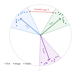
Comparison of Multimodal Embedding Models
The landscape of multimodal embedding models has evolved rapidly. Table 8 summarizes the key characteristics of the most influential models.
| Model | Modalities | Arch. | Dim. | Matryoshka | Key Innovation |
| CLIP [9] | Text, Image | Sep. | 512/768 | No | Large-scale contrastive |
| image-text pretraining | |||||
| [3pt] ALIGN [19] | Text, Image | Sep. | 640 | No | Noisy data at extreme |
| scale (1.8B pairs) | |||||
| [3pt] SigLIP [20] | Text, Image | Sep. | 768/1152 | No | Sigmoid loss replaces |
| softmax contrastive | |||||
| [3pt] BLIP-2 [21] | Text, Image | Sep. | 768 | No | Q-Former bridge |
| between modalities | |||||
| [3pt] CLAP [22] | Text, Audio | Sep. | 512 | No | Contrastive language- |
| audio pretraining | |||||
| [3pt] ImageBind [15] | 6 modalities | Sep. | 1024 | No | Image-anchored binding |
| of all modalities | |||||
| [3pt] Gemini Emb. [16] | 5 modalities | Uni. | 3072 | Yes | Native multimodal |
| with task conditioning |
Algorithm 8 (Multimodal Retrieval with Matryoshka Embeddings).
- Input: Multimodal corpus , embedding model , Matryoshka dimensions , candidate counts
- Output: Top- retrieval results for query
- Offline indexing:
- for each document
- Full embedding
- Store in coarse index
- Store in full index
- Online retrieval:
- Embed query
- Coarse retrieval: fast, low-dim
- for
- Re-rank with finer embedding
- return
The algorithm above illustrates the coarse-to-fine retrieval pipeline enabled by Matryoshka embeddings. The coarse stage uses low-dimensional prefixes for fast candidate generation over the entire corpus, while successive re-ranking stages use progressively higher-dimensional prefixes on progressively smaller candidate sets. This yields a total retrieval cost that is dominated by the coarse stage, with re-ranking adding negligible overhead.
Proposition 21 (Matryoshka Retrieval Speedup).
Let the ANN search cost be for dimension and corpus size (the typical scaling for locality-sensitive hashing). A two-stage Matryoshka retrieval with coarse dimension and fine dimension , retrieving candidates in the coarse stage, has total cost (Matryoshka Speedup) When , the speedup over single-stage retrieval at full dimension is approximately , which is substantial for large .
Several trends emerge from this comparison. First, the field is moving from bimodal (text-image only) to truly multimodal systems. Second, embedding dimensionality is increasing, reflecting the need to capture richer semantic information across more modalities. Third, the architectural trend is toward unified backbones rather than separate encoders, leveraging the internal multimodal representations of large foundation models. Fourth, Matryoshka representations are emerging as a practical necessity for production systems that must balance accuracy against latency and storage costs.
Exercise 38 (Modality Gap Measurement).
Download a pretrained CLIP model and compute embeddings for 1000 matched image-text pairs from the COCO Captions dataset.
Compute the modality gap using (Modality GAP). Is it positive?
Visualize the embeddings using t-SNE with perplexity 30. Do you observe separate modality clusters?
Compute the modality centroid directions and and measure the angle between them. How does this angle relate to the modality gap?
Apply PCA to remove the first principal component (which often captures the modality gap direction). Re-measure . Does the gap shrink? Does retrieval accuracy change?
Cross-Modal Retrieval
With multimodal embedding spaces established, we turn to the central capability they enable: cross-modal retrieval, the task of using a query in one modality to retrieve relevant results in another. This is not merely a technical exercise; it is a fundamental shift in how humans can interact with information. Instead of being confined to searching text with text queries or images with image queries, cross-modal retrieval allows a user to hum a melody and find the music video, sketch a rough drawing and find photographs, or describe a sound in words and find audio recordings.
The mathematical framework is a natural extension of single-modal retrieval to the cross-modal setting.
Definition 40 (Cross-Modal Retrieval).
Let and be the query and document modality spaces, with encoders and mapping to a shared embedding space. Given a query and a corpus , the cross-modal retrieval task returns the ranked list (Crossmodal Ranking) where is the inner product after -normalization (i.e., cosine similarity).
Text-to-Image and Image-to-Text Retrieval
Text-image retrieval is the most extensively studied cross-modal task, catalyzed by the success of CLIP [9] and the abundance of web-crawled image-text pairs. The task comes in two directions: text-to-image (given a caption, find the matching image) and image-to-text (given an image, find the matching caption).
These two directions are not symmetric in difficulty. Image-to-text retrieval is generally easier because a single image typically has many valid textual descriptions (a photograph of a dog in a park can be described as “a dog playing in the grass,” “a golden retriever in a park,” “an animal outdoors on a sunny day,” etc.), so the retrieval system has many correct targets. Text-to-image retrieval is harder because a specific textual description typically matches fewer images in the corpus.
Remark 31 (The Asymmetry of Cross-Modal Recall).
On standard benchmarks (Flickr30k, COCO), text-to-image Recall@1 is consistently 2–5 percentage points lower than image-to-text Recall@1 for the same model. This is not a model deficiency but a reflection of the one-to-many mapping from images to descriptions. For a corpus of images each with captions, the image-to-text task has correct answers per query but the text-to-image task has only 1 correct answer per query (or a small number, when multiple images share similar content). This combinatorial asymmetry inflates image-to-text recall relative to text-to-image recall.
The state-of-the-art approach follows a two-stage pipeline. In the embedding stage, both the query and all corpus items are encoded into the shared space. In the retrieval stage, approximate nearest neighbor (ANN) search identifies the top- candidates. The embedding stage is dominated by the encoder's computational cost (a forward pass through a Transformer), while the retrieval stage is dominated by the ANN search cost (sublinear in for tree-based or graph-based indices).
Proposition 22 (Hard Negative Mining for Cross-Modal Training).
Let be a matched query-document pair and be in-batch negatives. Define the hardness of a negative as . The gradient of the InfoNCE loss with respect to the query encoder parameters is (HARD NEG Gradient) where is the softmax weight over negatives. Hard negatives (large ) receive exponentially more gradient weight. This implies that the most informative training signal comes from negatives that the current model confuses with positives, not from trivially distinguishable negatives.
In practice, hard negative mining is critical for achieving strong cross-modal retrieval. Training with random negatives converges quickly to a “good enough” alignment but plateaus well below the performance achievable with carefully mined hard negatives. The most effective approach uses the current model to find hard negatives within a large candidate pool, then trains on batches enriched with these hard negatives.
For SigLIP [20], the contrastive loss is reformulated using a sigmoid function applied to each query-document pair independently, rather than the softmax over the batch used in CLIP. This removes the requirement for a global normalization across the batch and enables more stable training at very large batch sizes.
Text-to-Audio and Audio-to-Text Retrieval
The extension of contrastive alignment from the visual domain to audio produced CLAP (Contrastive Language-Audio Pretraining) [22], which learns a shared embedding space for text and audio. CLAP follows the same architectural blueprint as CLIP: a text encoder (typically a pretrained language model) and an audio encoder (typically a convolutional or Transformer model operating on mel-spectrogram inputs) are trained with contrastive loss on paired (text, audio) data.
The formal objective is identical to CLIP's InfoNCE loss, with the image encoder replaced by an audio encoder: (CLAP LOSS) where is the text encoder, is the audio encoder, are matched text-audio pairs, and is the batch size.
The unique challenges of text-audio retrieval include:
Temporal extent: Audio events unfold over time. A text description may refer to the overall scene (“a busy street”), a specific event (“a car horn honking”), or a temporal pattern (“footsteps gradually getting louder”). The audio encoder must capture temporal structure at multiple scales.
Polyphony: Natural audio contains multiple simultaneous sources. A recording of “birds singing in a forest with a stream” contains at least three overlapping sound classes. The embedding must represent this compositional structure.
Data scarcity: Compared to the billions of image-text pairs available on the web, text-audio pairs are orders of magnitude rarer. AudioCaps contains only 46k clips; Clotho contains only 5k.
Despite these challenges, CLAP enables compelling applications: natural language audio search (“find me the sound of rain on a tin roof”), audio captioning (generating text descriptions of audio), and zero-shot audio classification (classifying sounds using text labels without task-specific training).
Remark 32 (The Audio Embedding Landscape).
The audio modality occupies a curious middle ground between text and vision. Like text, audio is temporal and sequential. Like vision, audio is dense and continuous (when represented as a spectrogram). This dual nature means that audio embeddings can borrow techniques from both NLP (transformer architectures for sequential modeling) and computer vision (patch-based tokenization of spectrograms, treating them as “images”). The most successful audio encoders, including those used in CLAP and ImageBind, exploit this duality: they convert audio to mel-spectrograms and process them with architectures originally designed for images, while also using positional encodings that respect the temporal ordering of spectrogram patches. The fact that this “audio as image” approach works so well is itself evidence that the boundary between modalities is less fundamental than it appears.
Video-Text Retrieval
Video-text retrieval adds the dimension of temporal complexity. A video is not merely a collection of frames but a sequence of events, actions, and state changes that unfold over time. A text description of a video may refer to a single moment (“the cat jumps onto the table”), a temporal sequence (“first the chef chops onions, then adds them to the pan”), or a high-level summary (“a cooking tutorial for French onion soup”).
The computational challenge is also more severe. Encoding a video requires processing dozens to hundreds of frames. Naive approaches that encode every frame independently and aggregate the embeddings lose temporal information. More sophisticated approaches use temporal attention mechanisms, 3D convolutions, or video-specific Transformer architectures, but these increase computational cost proportionally.
Example 25 (Temporal Sensitivity in Video Retrieval).
Consider two videos: (A) a person picks up a cup, drinks from it, and puts it down; (B) a person puts down a cup, picks it up, and drinks from it. The same set of frames appears in both videos, but in different temporal order. A frame-level embedding that ignores temporal order would assign identical representations to both videos, yet the text descriptions “picking up a cup and drinking” and “putting down a cup, then picking it up” should retrieve different videos. This illustrates why temporal modeling is essential: the embedding must be order-sensitive, not just content-sensitive.
Historical Note.
From keyword search to semantic search to multimodal search. The evolution of information retrieval is a story of steadily expanding the definition of “relevance.” In the 1960s, keyword-based systems matched documents to queries by exact term overlap. In the 1990s, latent semantic indexing (LSI) introduced the idea that documents could be relevant even without sharing exact terms, by projecting both queries and documents into a low-dimensional space via SVD. In the 2010s, neural embeddings (Word2Vec, then BERT) made this projection learned and context-dependent. In the 2020s, multimodal embeddings extended relevance across modalities: an image can be “relevant” to a text query, a sound can be “relevant” to a visual query.
Each expansion required not just better algorithms but a broader theory of relevance. The mathematical frameworks evolved from Boolean logic (keyword matching) to linear algebra (LSI) to metric geometry (neural embeddings) to the cross-modal alignment theory we develop in this chapter. The common thread is the reduction of relevance to proximity in a learned space.
Any-to-Any Retrieval: The Ultimate Goal
The logical endpoint of multimodal embedding spaces is any-to-any retrieval: the ability to use a query in any modality to retrieve results in any other modality. With modalities, this subsumes all directed retrieval tasks (including intra-modal retrieval as a special case) under a single framework.
Definition 41 (Any-to-Any Retrieval System).
An any-to-any retrieval system is a tuple where:
is a set of modalities.
is a unified encoder (or a collection of aligned encoders) mapping any modality to a shared embedding space.
is a multimodal corpus, where is the sub-corpus for modality .
is a similarity function (e.g., cosine similarity).
For any query (any modality ), the system returns the ranked list over the entire multimodal corpus: (ANY TO ANY Ranking)
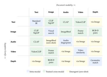
Zero-Shot Cross-Modal Transfer
The most intellectually satisfying capability of unified embedding spaces is zero-shot cross-modal transfer: performing retrieval between modality pairs for which no paired training data exists. ImageBind [15] demonstrates this concretely: given only (image, audio) and (image, text) training pairs, the model can perform audio-to-text retrieval without having seen a single audio-text pair.
This capability has profound implications for scalability. With modalities, direct pairwise alignment requires paired datasets. For (ImageBind's setting), that is 15 datasets. But with zero-shot transfer through an anchor modality, only datasets are needed (one per non-anchor modality paired with the anchor). The savings grow quadratically: for modalities, direct alignment needs 45 datasets versus only 9 for anchor-based alignment.
The mechanism is simple but profound. The image encoder creates a “bridge” in embedding space. An audio clip of a barking dog maps near the embedding of a photograph of a barking dog (because they were trained on image-audio pairs). The photograph of a barking dog maps near the embedding of the text “a dog barking” (because they were trained on image-text pairs). By transitivity, the audio clip maps near the text, enabling audio-to-text retrieval.
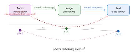
Lemma 6 (Transfer Loss Through the Bridge).
Let and be the alignment errors for modality to image and image to modality , respectively, measured on semantically matched inputs. The expected zero-shot cross-modal similarity satisfies (Transfer LOSS) The transfer loss (the reduction in expected similarity due to the indirection through the image bridge) is at most .
Proof.
By the triangle inequality on the unit sphere, for unit vectors : Using and similarly for the other term: Rearranging and taking expectations yields the stated bound.
The practical implication is that the transfer loss grows as the sum (not the product) of the individual alignment errors, plus a geometric mean term. If both pairwise alignments are good (), the transfer loss is at most , which implies a zero-shot similarity of at least . This is tight enough for many retrieval applications.
Information-Theoretic Limits of Cross-Modal Retrieval
We now ask a deeper question: given a fixed embedding dimension , what is the maximum possible retrieval performance? This is fundamentally an information-theoretic question, because the embedding acts as a lossy compression of the input, and the retrieval accuracy depends on how much information about the relevant document is preserved in the compressed representation.
The framework of rate-distortion theory [37][4] provides the right lens. We can view the embedding as a channel through which information about the query's semantic content is transmitted. The embedding dimension constrains the capacity of this channel.
Definition 42 (Embedding Channel Capacity).
Let be a random query and be its relevant document. The embedding functions and define an embedding channel from to the retrieved document . The embedding channel capacity is the maximum mutual information between the query and the retrieved document, optimized over all retrieval strategies: (Channel Capacity) where the supremum is over all encoder pairs mapping to , and is the nearest-neighbor retrieval result in the embedding space.
Theorem 8 (Embedding Bottleneck).
For -dimensional embeddings with -normalized vectors (i.e., embeddings lie on ), the mutual information between the query and the retrieved document is bounded by (Bottleneck Bound) where is the corpus size. For a corpus of documents in which exactly one is relevant, correct retrieval requires bits, yielding the minimum embedding dimension (MIN Dimension) For large , this simplifies to .
Proof sketch.
The key idea is that -dimensional unit sphere embeddings can encode at most bits of information about corpus membership, because the -covering number of is . To distinguish corpus items, we need the embeddings to be at least -separated, with .
More precisely, by a sphere-packing argument, the maximum number of non-overlapping spherical caps of angular radius on is bounded by the Rankin bound: . Setting and solving for the information content of the angular position yields the stated bound. The factor of arises from the Gaussian approximation to the cap volume in high dimensions.
Remark 33 (Practical Implications of the Bottleneck).
For a corpus of (one billion) documents, the theorem implies , which is trivially satisfied by modern embeddings (256 to 3072 dimensions). The theorem tells us that most of the embedding capacity in current systems is used for fine-grained discrimination, not for raw identification. This excess capacity is what enables approximate retrieval: even if the nearest-neighbor search is approximate (returning a result within a factor of of the true nearest neighbor), the rich geometry of the embedding space ensures that the result is still semantically close to the query.
Exercise 39 (Rate-Distortion Bound for Matryoshka Embeddings).
Consider a Matryoshka embedding with nested dimensions . For a corpus of documents:
Compute the embedding bottleneck bound ((Bottleneck Bound)) for each dimension .
At which dimension does the bound first exceed bits, the minimum information needed to uniquely identify the correct document?
In practice, retrieval accuracy improves well beyond the point where the information-theoretic minimum is met. Why? (Hint: the bound assumes adversarial corpus construction. Real corpora have structure.)
Downstream Applications of Foundational Embeddings
The preceding sections have developed the mathematical foundations of multimodal embedding spaces and cross-modal retrieval. Now we turn to the question that ultimately justifies all this theory: what can you build with it? The answer, it turns out, is astonishingly broad. Foundational embeddings are not merely a better search engine. They are a new computational primitive, a universal similarity function that can be composed, filtered, combined, and reasoned over to create applications that would have been inconceivable five years ago.
We survey established applications, then venture into speculative territory where the most exciting possibilities live.
Key Idea.
Embeddings as a Computational Primitive. A foundational embedding is not an application; it is a primitive, like addition or sorting, upon which applications are built. The key operations on this primitive are:
Similarity: compares any two inputs across any modalities.
Retrieval: finds the most relevant item in any corpus for any query.
Clustering: -means or spectral clustering on groups semantically related items regardless of modality.
Arithmetic: performs analogical reasoning in embedding space.
Interpolation: blends the semantics of two inputs.
Every application in this section is built from these five operations, composed in different ways for different purposes.
Creative Discovery and Artistic Exploration
The art world has always been organized by metadata: artist name, year, medium, movement, gallery. But the most interesting connections between artworks are often visual, connections that defy textual categorization. A Rothko color field and a Turner seascape share a luminous quality that no tag captures. A Hokusai wave and a Van Gogh night sky share a dynamic spiral energy that is felt rather than described.
Multimodal embeddings make these felt connections computable. By embedding artworks into a shared space, one can retrieve “paintings that feel like this one” without needing to articulate what “feel like” means. The embedding captures the visual gestalt, the holistic perceptual impression that resists decomposition into discrete attributes.
But the truly novel capability is cross-modal creative retrieval. Given a piece of music, find paintings that evoke the same mood. Given a poem, find photographs that capture the same atmosphere. Given a perfume description (“woody, with notes of cedar and a hint of vanilla”), find visual artworks that evoke the same sensory palette. These queries are absurd in a keyword-based system. In a multimodal embedding space, they are just nearest neighbor searches.
Example 26 (Synesthetic Art Curation).
A museum curator wants to design an exhibition called “The Sound of Blue,” pairing visual artworks with musical compositions. Using a multimodal embedding model:
Embed all visual artworks in the collection (12,000 paintings and sculptures, photographed and embedded as images).
Embed a curated library of musical compositions (5,000 tracks, embedded as audio).
For each artwork, retrieve the 5 nearest musical compositions in embedding space.
For each piece of music, retrieve the 5 nearest artworks.
The curator reviews these pairings, selecting those that resonate artistically, a human-AI collaboration where the embedding model proposes and the curator disposes.
The result is an exhibition where visitors hear music that “matches” each painting, not through explicit programming but through the emergent geometry of a shared semantic space.
Accessibility Through Retrieval
For the 2.2 billion people worldwide with vision impairment, the visual world is mediated by descriptions. Alt text on web images, screen reader outputs, and audio descriptions of videos are critical accessibility tools, but they are expensive to produce manually and are missing for the vast majority of visual content.
Embedding-based retrieval offers a scalable alternative. Given an image that lacks a description, retrieve the most similar image in a database of described images, and transfer its description. The key insight is that descriptions do not need to be generated from scratch; they can be retrieved from a large pool of existing descriptions.
Key Idea.
Retrieval-Augmented Description. For an undescribed image , compute its embedding . Retrieve the nearest described images from a reference database: where is the text description of image . The transferred description is a function of the retrieved descriptions: (Transferred Description) where is the similarity score and is an aggregation function (e.g., the description of the nearest neighbor, or an LLM-generated summary of the top- descriptions weighted by similarity).
This approach has a crucial advantage over pure generation: the descriptions are grounded in human-written text, reducing the risk of hallucinated or misleading content. A visually impaired user receives a description that was written by a human for a visually similar image, not fabricated by a model that might confuse a cat for a dog.
The same principle extends to audio accessibility. A deaf user encountering a video can benefit from retrieved descriptions of similar audio tracks. If the video's soundtrack is similar (in embedding space) to a previously described audio clip, the existing description can be transferred: “sounds of traffic and distant sirens” provides environmental context that a visual-only experience cannot convey. Cross-modal retrieval thus becomes a bridge between sensory experiences, using the information available in one modality to augment the experience of another.
Content Moderation at Scale
Content moderation is one of the most consequential applications of embedding-based retrieval. Platforms hosting user-generated content must identify and remove harmful material, including known child sexual abuse material (CSAM), violent extremist content, copyright-infringing material, and spam, at a scale of billions of uploads per day.
The traditional approach uses perceptual hashing (e.g., PhotoDNA for images, MD5 hashes for exact duplicates), which matches against a database of known harmful content. Perceptual hashes are fast and deterministic but brittle: a simple crop, resize, or color shift can evade detection.
Embedding-based retrieval replaces the hash with a learned representation that is robust to superficial transformations. A harmful image and its cropped, resized, or color-shifted variant map to nearby points in embedding space, enabling detection even when the content has been deliberately modified to evade hash-based systems.
Caution.
Bias in embedding-based moderation. Embedding models inherit biases from their training data. Studies have shown that CLIP-based embeddings associate certain demographics with harmful content at higher rates than others, reflecting biases in the web-crawled training data. A content moderation system built on biased embeddings will over-flag content from underrepresented groups and under-flag content from overrepresented groups. This is not a hypothetical risk; it has been documented in deployed systems [9]. Any production deployment of embedding-based moderation must include bias auditing, per-group false-positive rate monitoring, and human review for edge cases.
Scientific Discovery Across Modalities
Science communicates through a rich multimodal fabric: papers contain text, equations, figures, tables, and citations; datasets contain numbers, images, and metadata; presentations contain slides, speech, and video. Traditional scientific search operates almost exclusively on text (titles, abstracts, keywords), leaving the vast majority of scientific content unsearchable.
Multimodal embeddings open the door to searching the full fabric of scientific communication. Consider these scenarios:
Figure-to-paper retrieval: A researcher has a figure from a conference talk but cannot remember which paper it came from. Embed the figure, search against a database of paper figures, retrieve the source paper.
Text-to-figure retrieval: A researcher writing a survey wants to find all published figures that visualize “attention weights in transformer models.” A text query retrieves relevant figures from across the literature.
Equation-to-paper retrieval: A researcher encounters an equation and wants to find its origin or related work. If equations are rendered as images, they can be embedded and matched against a database of equation images from published papers.
Data-to-method retrieval: Given a dataset's characteristics (embedded as a structured description), retrieve papers that have achieved good results on similar datasets.
Open Problem 3.
Open problem: Embedding scientific equations. Equations are the most information-dense modality in scientific communication, yet they are poorly served by current embedding models. An equation like is not “an image” (it has precise symbolic structure), not “text” (it uses mathematical notation that NLP tokenizers mangle), and not “structured data” (it has semantic meaning beyond its syntactic form). Developing embedding models that natively understand the structure and semantics of mathematical notation, mapping equations with the same mathematical content but different notational conventions to nearby points, is an open problem with enormous potential impact on scientific information retrieval.
Multimodal Product Search
E-commerce was among the first industries to deploy multimodal embeddings at scale. The use case is intuitive: a customer sees a pair of shoes on the street, takes a photograph, and searches for similar products. Or a customer describes what they want in natural language: “a mid-century modern coffee table in walnut with tapered legs.” Or a customer provides an image of their living room and asks for furniture that would “go with” the existing decor.
Each of these queries leverages a different modality (image, text, or image-as-context), but all are resolved by the same mechanism: embed the query, search the product embedding index, return the nearest neighbors.
The commercial impact is substantial. Visual search increases conversion rates by 30–50% compared to text-only search for categories where visual appearance dominates the purchase decision (fashion, furniture, home decor). Multimodal search, combining text and image cues, performs even better because it captures both the visual gestalt and the specific attributes the customer cares about.
Example 27 (Hybrid Text-Image Product Queries).
A customer uploads a photograph of a blue ceramic vase and adds the text “something like this but taller and in terracotta.” The retrieval system must combine two signals: the visual similarity to the photograph (shape, texture, style) and the textual modification (taller, terracotta). One approach embeds the image and text separately, then combines them: (Hybrid Query) where controls the balance between visual and textual cues. A more sophisticated approach uses a cross-attention mechanism that conditions the image embedding on the text, allowing the text to “edit” the visual query in embedding space. The latter approach better handles instructions like “same shape but different color,” where the text specifies which visual attributes to preserve and which to modify.
Remark 34 (Cold Start in Product Search).
New products present a cold-start problem for recommendation systems but not for embedding-based search. A product with zero purchase history and zero clicks can still be retrieved if its image and description produce an embedding close to the user's query. This is a fundamental advantage of content-based retrieval (via embeddings) over collaborative filtering: relevance is determined by the intrinsic properties of the product, not by the behavior of other users. For platforms with rapidly changing catalogs (fashion retailers adding hundreds of new items daily), this property is essential.
Cross-Modal Medical Retrieval
The medical domain presents a particularly compelling case for cross-modal retrieval because clinical decision-making inherently involves multiple modalities: radiology images (X-rays, CT scans, MRIs), clinical notes (free text), laboratory results (structured data), pathology slides (microscopy images), and patient histories (longitudinal text).
Example 28 (Case-Based Diagnostic Retrieval).
A radiologist examines a chest X-ray showing an unusual opacity. Using a cross-modal retrieval system, they can:
Image-to-image: Find prior chest X-rays with similar opacities, along with their confirmed diagnoses.
Image-to-text: Retrieve clinical notes from cases with similar imaging findings, providing context on symptoms, comorbidities, and outcomes.
Text-to-image: Query “ground-glass opacity in the right lower lobe with pleural effusion” and retrieve matching images from the hospital's archive.
Multimodal-to-multimodal: Combine the X-ray image with the patient's clinical notes to retrieve the most similar complete cases (image + text jointly).
This is not a replacement for clinical judgment; it is evidence-based medicine operationalized as nearest-neighbor search in embedding space.
The privacy implications are severe. Medical embeddings must be designed so that patient-identifying information cannot be reconstructed from the embedding vector, even under adversarial attack. This connects to the broader field of privacy-preserving embeddings, where differential privacy or adversarial debiasing techniques are applied during embedding training to ensure that sensitive attributes are not encoded in the representation.
Definition 43 (Privacy-Preserving Embedding).
A privacy-preserving embedding satisfies -differential privacy if for any two inputs differing in a single patient attribute, and any measurable set : (DP Embedding) The privacy-utility tradeoff is governed by the relationship between (privacy budget), (embedding dimension), and retrieval accuracy: lower provides stronger privacy but degrades the embedding's discriminative power.
The formal tension between privacy and utility in medical embeddings is a special case of a fundamental information-theoretic tradeoff. The embedding must contain enough information to discriminate between different medical conditions (for retrieval to be useful) but not enough to identify individual patients (for privacy to be maintained). Formalizing this tradeoff and finding the Pareto frontier between privacy and retrieval accuracy is an active area of research with significant clinical implications.
Beyond the Horizon: Visionary Applications
The applications surveyed above are either deployed or under active development. We now venture into more speculative territory, exploring applications that become conceivable, even if not yet practical, once we take the premises of multimodal embedding spaces to their logical conclusion. These are not idle fantasies; each follows directly from capabilities that current embedding models either already possess or are close to possessing.
Emotional Retrieval.
Emotions are arguably the most important human information modality, yet they are absent from every information retrieval system ever built. What if we could embed emotional states? A user listens to a piece of music that makes them feel melancholy. They want to find a painting that evokes the same feeling, or a poem, or a scene from a film. This is not text search (“find sad paintings”) but something deeper: the query is not a text label of the emotion but the emotion itself, as evoked by a specific sensory experience.
The path to emotional retrieval lies in the observation that multimodal embeddings already capture some emotional information. CLIP embeddings of images rated as “serene” by human annotators cluster together in embedding space, separated from images rated as “anxious” or “joyful.” This is not because CLIP was trained on emotion labels; it is because the visual features that evoke serenity (soft colors, open spaces, horizontal compositions) are correlated with the text descriptions that appear alongside such images on the web. Emotional information is already latent in the embedding geometry.
The research challenge is to amplify this latent emotional signal. Fine-tuning on emotion-annotated datasets, incorporating physiological signals (heart rate, galvanic skin response) as additional modalities, or training on affective descriptions (“this image makes me feel calm”) rather than factual ones (“a sunset over the ocean”) could produce embeddings where the emotional dimension is a first-class citizen rather than an incidental byproduct.
Thought Retrieval.
If emotional retrieval seems speculative, thought retrieval borders on science fiction, but the boundary is narrower than one might expect. Recent work in neural decoding has demonstrated that fMRI signals recorded while a subject views an image can be decoded into a representation that, when projected into CLIP embedding space, correctly identifies which image the subject was viewing from a set of candidates. The brain activity is literally being embedded into the same space as images and text.
Extend this to retrieval: a subject thinks of a visual concept, a face, a landscape, an object. Their brain activity is recorded (via fMRI, EEG, or a future non-invasive neural interface), embedded into the multimodal space, and used as a query. The system retrieves images, sounds, or text that match the subject's mental imagery. This is not content-based retrieval in the traditional sense; it is intention-based retrieval, where the query is the user's thought itself.
Insight.
The Embedding Space as a Universal Lingua Franca. The deep significance of thought retrieval is not the specific application but the principle it reveals. The multimodal embedding space is becoming a universal lingua franca for information, a space in which any form of meaning, whether expressed as text, image, sound, or neural activity, can be represented, compared, and translated. The embedding dimension is the bandwidth of this universal language. As grows and training data spans more modalities, the embedding space converges toward a representation of meaning itself, stripped of the accidents of its physical encoding.
Cross-Temporal Retrieval.
History is filled with recurrence. A medieval siege and a modern urban warfare scenario share tactical patterns. A 17th-century financial bubble and a 21st-century cryptocurrency crash follow similar dynamics. An Art Deco building facade and a modern minimalist building share geometric sensibilities that transcend their 80-year separation.
Cross-temporal retrieval uses embeddings to find these connections across time. Given a historical artifact (a photograph, a document, a map), retrieve its modern analog: the contemporary object, event, or concept that is most semantically similar. This requires embeddings that capture abstract patterns rather than surface features, embeddings that recognize the structural similarity between a Roman aqueduct and a modern pipeline, or between a medieval manuscript's illumination and a modern infographic's design language.
The educational potential is immense. Imagine a history student who can point their camera at a museum artifact and instantly see its modern parallels, not through manually curated links but through the emergent geometry of a well-trained embedding space.
Example 29 (Architectural Analogy Retrieval).
A database contains photographs of 50,000 historical buildings (ancient through modern) with metadata. A user photographs a Roman arch and queries for modern analogs. The embedding model, trained on diverse architectural imagery, places the Roman arch near modern structures that share its key geometric features: parabolic curves, load-bearing masonry, monumental scale. The top retrievals include a modern concrete shell structure by Félix Candela, a Santiago Calatrava bridge, and a contemporary museum entrance. None of these would be found by keyword search on “Roman architecture”; the connection is purely visual and structural, captured by the embedding geometry. The system has effectively learned an architectural “grammar” that transcends historical period.
Synesthetic Retrieval.
Synesthesia, the neurological phenomenon in which stimulation of one sense triggers an involuntary experience in another (seeing colors when hearing music, tasting shapes), has long fascinated artists and scientists. Multimodal embedding spaces make synesthetic associations computable.
What does the color blue sound like? In a well-trained multimodal embedding space, one can embed images of blue objects, retrieve the nearest audio clips, and listen to what the model “thinks” blue sounds like. What does a C-major chord look like? Embed the chord as audio, retrieve the nearest images. These queries exploit the cross-modal geometry of the embedding space to create synesthetic mappings that are data-driven rather than arbitrary.
Whether these computed synesthetic associations align with the experiences of human synesthetes is an open empirical question, one that connects computational embedding theory to the neuroscience of cross-modal perception.
Dream Indexing.
The most speculative application of all: indexing the content of dreams. As neural decoding technology advances from fMRI (expensive, slow, low temporal resolution) toward high-density EEG or optical neural interfaces (potentially portable and real-time), it becomes conceivable to record brain activity during REM sleep and embed the resulting signals into a multimodal space. The “dream embedding” would sit near images, sounds, and narratives that resemble the dream content. Upon waking, the dreamer could query their dream log: “Show me what I dreamed about last Tuesday” would return a collage of images, sounds, and text fragments that the embedding model associates with the recorded neural activity.
This application is decades away, if it is possible at all. But it illustrates the ultimate promise of multimodal embedding spaces: if any signal, from any source, can be embedded into the same space, then the space becomes a universal index of human experience.
Embedding-Mediated Translation.
A more near-term visionary application is embedding-mediated translation between modalities. Rather than training a separate generative model for each modality pair (text-to-image, image-to-audio, audio-to-video, etc.), one trains a single conditional generator that takes an embedding vector as input and produces output in a specified target modality. The embedding serves as the modality-agnostic representation of “what to generate,” and the generator handles the “how.”
Definition 44 (Embedding-Mediated Generation).
An embedding-mediated generator for modality is a function that maps embedding vectors to outputs in modality . Given an input from any source modality , the cross-modal generation pipeline is: (EMB Mediated GEN) where is the multimodal encoder and is the modality-specific generator. This decouples the understanding of “what” (handled by ) from the generation of “how” (handled by ), and enables cross-modal generation between any pair of modalities with only generators rather than translation models.
This architecture reduces the translation problem to generation problems, each conditioned on the same embedding space. The embedding space serves as the interlingua, the intermediate representation through which all modality pairs communicate.
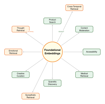
Open Problems and Research Frontiers
Open Problem 4.
Open problems in foundational embedding applications.
Compositional retrieval: Current embeddings represent holistic semantics well but struggle with compositional queries like “a red car next to a blue truck” (they may retrieve a blue car next to a red truck). How can embeddings be made compositionally faithful?
Temporal dynamics in embeddings: The world changes, and so should embeddings. A photograph of the World Trade Center has fundamentally different semantic associations before and after September 2001. How should embedding models handle temporal context?
Cultural grounding: Embeddings trained on English-language web data embed Western cultural associations. A model might associate “wedding” with white dresses rather than red saris. How can embeddings be culturally pluralistic?
Embedding forensics: Given only an embedding vector, can one determine which model produced it, what input it encodes, or whether it has been adversarially perturbed? This is the embedding analog of image forensics.
Continual embedding learning: Production corpora grow continuously. How can embedding models be updated to incorporate new concepts without catastrophic forgetting of existing representations?
Grounding in physical interaction: Current embeddings capture appearance and description but not affordance. A hammer and a rock may serve the same function (driving a nail in an emergency) but look nothing alike. Can embeddings capture functional similarity alongside perceptual similarity?
Theoretical limits of cross-modal alignment: What is the information-theoretic limit on how well two modalities can be aligned given finite paired data? Is there an analog of the Bayes error rate for cross-modal retrieval?
Caution.
Bias amplification in embedding-based retrieval. Retrieval systems do not merely reflect the biases in their training data; they amplify them. This amplification occurs through a feedback loop: biased embeddings produce biased retrieval results, which are presented to users, who interact with them (clicking, saving, sharing), generating interaction data that is used to fine-tune the next generation of embeddings. Each iteration tightens the bias.
Formally, let be the initial bias in the embedding space (measured, e.g., as the differential association between a demographic group and positive versus negative content). After rounds of the deploy-collect-retrain cycle, the bias amplifies to approximately for a positive amplification rate that depends on the user interaction model. Even small initial biases () can grow to problematic levels () within a few retraining cycles.
Mitigations include: (a) bias auditing at each retraining cycle, (b) counterfactual data augmentation to balance demographic representation, (c) adversarial debiasing objectives during embedding training, and (d) post-hoc calibration of retrieval scores across demographic groups. None of these is sufficient alone; responsible deployment requires all four.
Exercise 40 (Building a Cross-Modal Retrieval System).
Using a pretrained multimodal embedding model (e.g., CLIP or an open-source ImageBind implementation), build a cross-modal retrieval system:
Index construction: Download a multimodal dataset (e.g., AudioCaps for audio-text, or Flickr30k for image-text). Embed all items and build a FAISS index for approximate nearest neighbor search.
Text-to-image retrieval: Given a text query, retrieve the top-5 images. Measure Recall@1 and Recall@5 on the test set.
Image-to-text retrieval: Given an image query, retrieve the top-5 text descriptions. Compare performance with text-to-image. Is the asymmetry described in Remark 31 present?
Matryoshka experiment: If using a model with Matryoshka embeddings, repeat the retrieval experiments at dimensions 256, 768, and 3072. Plot Recall@1 versus dimension. At what dimension does performance plateau?
Bias audit: For a subset of queries related to people (e.g., “a person cooking”), examine the retrieved images. Is there evidence of demographic bias in the results? Propose a quantitative metric to measure this bias.
Exercise 41 (Emergent Zero-Shot Retrieval).
Using ImageBind (or an equivalent model supporting audio and text):
Embed 100 audio clips and 100 text descriptions from different domains (e.g., AudioCaps for audio, hand-written descriptions for text).
Perform audio-to-text retrieval: for each audio clip, retrieve the nearest text description. Evaluate the quality of matches manually on a 1–5 scale.
Compare the zero-shot audio-to-text performance with the direct audio-to-image and image-to-text performance. Is the transfer loss consistent with the bound in Lemma 6?
Propose an experiment to test whether longer transfer chains (e.g., audio image text video) degrade more rapidly than the lemma predicts.
Conjecture 1 (The Universal Embedding Hypothesis).
There exists a finite embedding dimension such that all human-perceptible semantic distinctions can be faithfully represented on . That is, for any two inputs (in any modality) that a human judge would consider semantically different, a sufficiently well-trained universal embedding model assigns them representations with cosine similarity below a threshold , and for any two inputs that a human judge would consider semantically identical, the model assigns representations with cosine similarity above .
If this conjecture is true, the question shifts from “can we build a universal embedding?” to “what is ?” Current evidence suggests , but determining even an order-of-magnitude estimate remains an open problem. The conjecture connects to deep questions in cognitive science about the dimensionality of human semantic representation, and to information-theoretic questions about the intrinsic dimensionality of “meaning.”
This conjecture, if true, would imply that the era of modality-specific retrieval is a temporary phase in the history of information systems. The destination is a single embedding space, a single index, and a single retrieval mechanism for all forms of human information. The mathematical foundations developed in this chapter, from contrastive alignment to rate-distortion bounds to modality gap analysis, are the tools that will either prove or disprove this conjecture, and that will guide the engineering of the universal retrieval systems of the future.
Exercise 42 (Modality Gap Reduction Strategies).
The modality gap (The Modality Gap Problem) reduces retrieval accuracy because it biases the nearest-neighbor search toward same-modality results. Consider the following strategies for reducing the gap:
Post-hoc centering: Subtract each modality's centroid from its embeddings: . Re-normalize to the unit sphere. Does this eliminate the gap? What information might be lost?
Shared projection head: Add a shared linear projection after all modality encoders, trained to minimize the modality gap while preserving intra-modal discriminability. Formulate this as an optimization problem with two competing objectives.
Adversarial modality confusion: Train a modality classifier on top of the embeddings (“given this embedding, which modality produced it?”) and add its negative cross-entropy to the training loss, encouraging embeddings that are modality-agnostic. Why might this approach harm retrieval accuracy if applied too aggressively?
Theoretical analysis: Using Theorem 7, derive conditions under which strategy (a) provably reduces the gap to zero. Under what conditions does it fail?
Exercise 43 (Information Content of Embeddings).
This exercise explores the practical implications of the embedding bottleneck theorem (Theorem 8).
For a corpus of images, compute the minimum embedding dimension required for unique identification. Compare this with the dimensions used by CLIP (512), ImageBind (1024), and Gemini Embedding (3072).
The theorem assumes worst-case corpus construction. In practice, natural image corpora have structure (e.g., images of cats cluster together). Argue informally that this structure allows retrieval to succeed at dimensions much lower than .
Design an experiment to estimate the effective dimensionality of a real embedding space: the number of dimensions that carry meaningful variance. (Hint: PCA on a large set of embeddings.) How does the effective dimensionality compare with the nominal dimensionality?
If we quantize each embedding coordinate to bits (e.g., for int8 quantization), the total information capacity is bits. For CLIP at , (float32), this is 16,384 bits. How does this compare with for a billion-document corpus? What does the excess capacity buy us?
Generative Reranking
You have one thousand potentially relevant documents. A simple scorer, perhaps BM25 or a bi-encoder, ranked them in a fraction of a second. But a large language model can understand nuance, context, and intent in ways that a bag-of-words statistic or a dot product in embedding space simply cannot. Can the LLM rerank those documents more accurately? Yes, and this insight is transforming the entire retrieval pipeline.
The idea is disarmingly simple: take the candidate list produced by a cheap first-stage retriever, then use a more powerful (and more expensive) model to refine the ordering. The first-stage retriever provides recall: it finds documents that might be relevant. The reranker provides precision: it puts the truly relevant documents at the top. This two-stage pattern, sometimes called retrieve-then-rerank, has become the dominant architecture in modern information retrieval.
What makes recent work exciting is the realisation that generative language models, models trained to produce text rather than classify it, can serve as extraordinarily effective rerankers. The key distinction lies in how the model processes the query and document, and how many documents it considers at once. This distinction gives rise to four paradigms: pointwise, pairwise, listwise, and setwise reranking.
Pointwise Reranking
The simplest approach scores each document independently. Given a query and a candidate document , the reranker produces a relevance score without reference to any other document in the candidate set. The final ranking is obtained by sorting documents by their scores.
Definition 45 (Pointwise Reranker).
A pointwise reranker is a function that assigns a relevance score to each query-document pair independently. Given a candidate set , the reranked list is the permutation satisfying (Pointwise Ranking)
Cross-Encoders with BERT
The cross-encoder architecture, introduced in the context of natural
language inference and adapted for retrieval, concatenates the query
and document into a single input sequence and passes it through a
Transformer encoder [83]. The [CLS] token
representation is fed to a classification head that outputs a
relevance score:
(Cross Encoder)
where is a learned projection and is a scalar
bias. The critical advantage over bi-encoders is that the query and
document tokens attend to each other throughout every Transformer
layer, enabling fine-grained interaction modelling. The critical
disadvantage is computational cost: a separate forward pass is
required for every query-document pair.
Remark 35.
For a candidate set of documents, the cross-encoder requires forward passes, each with sequence length proportional to . In contrast, a bi-encoder computes query and document embeddings independently, requiring only a single dot product per candidate at query time. This cost asymmetry is precisely what motivates the two-stage retrieve-then-rerank architecture: the bi-encoder handles the bulk filtering, and the cross-encoder refines a much smaller candidate set.
monoT5: Sequence-to-Sequence Relevance Scoring
Nogueira et al. [84] proposed a remarkably elegant reformulation: instead of adding a classification head to an encoder, use a sequence-to-sequence model and ask it to generate a relevance judgment. Given query and document , the input to T5 [85] is:
Query: $q$ Document: $d$ Relevant:
The model generates either “true” or “false” as output. The relevance score is derived from the probability assigned to the “true” token: (Monot5 Score)
This formulation is powerful for two reasons. First, it leverages the pre-trained knowledge encoded in T5's parameters: the model has already seen billions of tokens and developed a rich understanding of relevance, topicality, and semantic similarity. Second, it requires no architectural modifications; any sequence-to-sequence model can serve as a pointwise reranker with this prompt template.
Example 30 (monoT5 in Practice).
Consider the query “What causes tides?” and two candidate documents:
: “Tides are caused by the gravitational pull of the Moon and, to a lesser extent, the Sun on Earth's oceans.”
: “The Tide brand of laundry detergent was introduced by Procter & Gamble in 1946.”
A BM25 scorer might rank both documents similarly, since both contain the word “tide.” But monoT5, processing the full query-document context, assigns and , correctly distinguishing the oceanographic sense from the commercial one.
Pairwise Reranking
Pointwise reranking treats each document in isolation. But relevance is often relative: document might be hard to judge on its own, but clearly more relevant than document when the two are compared side by side. Pairwise reranking exploits this observation.
Definition 46 (Pairwise Reranker).
A pairwise reranker is a function that, given a query and two documents , returns the probability that is more relevant than : (Pairwise Score) A full ranking is obtained by aggregating pairwise preferences, for example via a sorting algorithm that uses as its comparison function.
duoT5: Pairwise Comparison via Generation
The duoT5 model extends the monoT5 idea to the pairwise setting. Given a query and two documents, the T5 model receives:
Query: $q$ Document0: $d_A$
Document1: $d_B$ More relevant:
The model generates either “Document0” or “Document1,” and the comparison score is: (Duot5 Score)
Remark 36.
A subtle issue with pairwise reranking is that the preference function need not be transitive. It is possible that and but , forming a preference cycle. In practice, this is rare for well-calibrated models, but sorting algorithms that assume transitivity may produce inconsistent results. The Copeland voting rule, which ranks documents by the number of pairwise victories, is a robust aggregation strategy that handles non-transitive preferences gracefully.
The principal drawback of pairwise reranking is computational. Ranking documents requires pairwise comparisons in the worst case. Even with efficient sorting algorithms that require only comparisons, each comparison involves a full forward pass through the language model. For large candidate sets, this cost is prohibitive.
Listwise Reranking
The natural next step is to process the entire candidate list at once. Instead of scoring documents individually or comparing them in pairs, a listwise reranker receives the query and all candidate documents simultaneously and produces a permutation of the entire list.
Definition 47 (Listwise Reranker).
A listwise reranker is a function that maps a query and an ordered list of candidate documents to a permutation , where is the symmetric group on elements. The reranked list places document first, second, and so on.
LLM Permutation Generation
Hou et al. [24] demonstrated that large language models can directly generate permutations. The prompt presents the query and a numbered list of document passages, then asks the LLM to output the passage numbers in order of decreasing relevance. For example:
I will provide a query and a list of passages.
Rank the passages based on their relevance to the query.
Output the ranking as a list of passage numbers from most
to least relevant.
Query: $q$
Passage [1]: $d_1$
Passage [2]: $d_2$
Passage [$n$]: $d_n$
Ranking:
The model generates a sequence such as “[3] > [1] > [5] > [2] > [4],” which is parsed into the permutation .
The appeal of listwise reranking is that the model can consider all documents simultaneously, making globally coherent comparisons. The challenge is context length: a list of even 20 moderately long passages may exceed the context window of many language models, and attention cost grows quadratically with sequence length.
Sliding Window Approaches
To handle lists longer than the context window allows, sliding window strategies partition the candidate list into overlapping windows and rerank each window independently. The results are then merged using a bubble-sort-like procedure: the top-ranked document from the current window is compared against documents in the next window, and the process repeats until the entire list has been processed.
Algorithm 9 (Sliding Window Listwise Reranking).
- Input: Query ; candidate list ; window size ; step size ; listwise reranker
- Output: Reranked list
- input ordering
- for convergence
- for slide from bottom to top
- extract window
- rerank window
- apply permutation
- return
The sliding window approach trades optimality for tractability. Each window reranking is a local operation, and relevant documents gradually “bubble up” through the list across multiple passes. In practice, two to three passes suffice for most applications, and the approach scales to lists of hundreds or thousands of documents.
Lemma 7 (Convergence of Sliding Window Reranking).
Let be the true relevance-based permutation, and let be the permutation produced after passes of the sliding window algorithm with window size and step size . If the listwise reranker produces the correct ordering within each window with probability at least , then after passes, the top- documents are correctly ranked with probability at least .
Proof.
After one complete bottom-to-top pass, the most relevant document in the entire list has been compared against every other document through overlapping windows. If each window is correctly ranked (probability per window), the most relevant document “bubbles” to position 1. By induction, after passes, the top- documents have had the opportunity to be correctly positioned. The probability that all window rankings in a single pass are correct is at least by a union bound, giving the stated guarantee after passes by independence across passes.
Remark 37.
The sliding window approach is structurally analogous to bubble sort, where adjacent elements are compared and swapped. Just as bubble sort requires passes in the worst case, the sliding window reranker may require multiple passes to propagate a highly relevant document from the bottom of the list to the top. However, because the initial ordering is already a reasonable ranking (provided by the first-stage retriever), the number of required passes is typically much smaller than the worst case.
Setwise Reranking: The Efficiency Frontier
Pointwise reranking requires LLM calls. Pairwise reranking requires calls at minimum and in the worst case. Listwise reranking requires only a single call for the entire list, but is limited by context length. Setwise reranking, introduced by Zhuang et al. [23], occupies a sweet spot between these extremes.
Definition 48 (Setwise Reranker).
A setwise reranker operates by repeatedly presenting the query alongside a subset of candidate documents and asking the LLM to identify the most relevant document in . The selected document is placed at the top of the output ranking and removed from the candidate pool. The process repeats with the remaining candidates until all documents have been ranked. Formally, at each step : (Setwise Selection) where is a subset of size drawn from the remaining candidates , and is the probability that the LLM identifies document as the most relevant in .
The key insight is that the LLM processes only documents per call, keeping the context length manageable, while the selection procedure produces a globally meaningful ranking. The subset is typically chosen to include the top candidates from the remaining pool according to the first-stage retriever's scores.
Algorithm 10 (Setwise LLM Reranking).
- Input: Query ; candidate set with initial scores; subset size ; number of documents to rank
- Output: Top- reranked list
- empty ranked list
- candidates
- for
- select candidates by initial score
- Construct prompt: “Given query and documents , which is most relevant?”
- decode most probable document identifier
- Append to
- return
Proposition 23 (Setwise Ranking Reduces LLM Calls).
To rank the top documents from a candidate set of size using setwise reranking with subset size , the number of LLM calls is exactly , each processing documents. In contrast, pairwise reranking requires LLM calls for a complete ranking, and calls for the top- ranking via selection. The setwise approach therefore reduces LLM calls from to with a per-call cost proportional to .
Proof.
At each of the iterations, the setwise algorithm makes exactly one LLM call that processes documents. Thus the total number of LLM calls is .
For pairwise reranking via repeated selection (analogous to selection sort), finding the top-ranked document requires comparisons, the second-ranked requires , and so on. The total number of pairwise comparisons for the top documents is: (Pairwise Calls) Each comparison requires one LLM call. Therefore, the setwise approach uses calls compared to for pairwise selection, a reduction by a factor of .
When is fixed, each setwise LLM call processes document passages, so the total token cost is , which for is dramatically cheaper than the token cost of pairwise selection.
Remark 38.
The quality of setwise ranking depends on the subset size . If , setwise reranking degenerates to pairwise comparison with a single-elimination tournament structure. If , it becomes listwise reranking. Empirically, in the range 5 to 20 provides a good balance between efficiency and ranking quality.
Example 31 (Setwise Reranking for Legal Search).
Consider a legal researcher querying “precedent for employer liability in remote work injuries.” A BM25 retriever returns 100 candidate case documents. The setwise reranker with selects the 10 top-scoring candidates, presents them to the LLM alongside the query, and asks which case is most relevant. The LLM, understanding that “remote work injuries” requires cases about workplace injury law in non-traditional settings (not just keyword overlap with “remote” or “work”), selects a 2021 workers' compensation ruling involving a home office accident. This document is placed first in the output ranking, and the process repeats with the remaining 99 candidates. After 10 iterations, the top-10 ranking is complete, having required only 10 LLM calls rather than the 100 needed by pointwise reranking.
FIRST: Fast Listwise Ranking via Single Tokens
Listwise reranking with LLMs typically requires the model to generate an entire permutation as a sequence of tokens. FIRST (Fast lIstwise Ranking via Single Token decoding) [86] observes that if we only need to identify the top document, we can do so by examining the logits over a single token position.
The idea is as follows. Present the LLM with the query and passages, each labelled with a single-character identifier (A, B, C, ). Then ask the model: “The most relevant passage is:” and examine the probability distribution over the next token. The passage whose identifier receives the highest probability is deemed most relevant: (First Score) where is the character identifier for passage .
Key Idea.
One Token Is All You Need The probability distribution over a single decoded token implicitly encodes the model's ranking of all passages. By examining this distribution rather than generating a full permutation sequence, we reduce decoding latency from autoregressive steps to a single forward pass. This is especially valuable when using large models where each decoding step is expensive.
To rank all documents (not just the top one), FIRST combines single-token decoding with a selection procedure similar to the setwise approach: identify the best document in the current window, remove it, and repeat. Alternatively, the probability distribution over all identifiers can be used directly as scores, though this requires careful calibration.
Remark 39.
A subtlety of single-token decoding is that the logit distribution over passage identifiers is not necessarily well calibrated. The LLM may assign disproportionate probability mass to identifier “A” simply because it appears first in the prompt (position bias), not because passage A is most relevant. Zhuang et al. [23] address this by averaging across multiple random permutations of the passage ordering in the prompt, a technique called permutation calibration. Specifically, for random orderings of the passages: (First Calibrated) where is the identifier assigned to document under permutation . This averaging eliminates position bias at the cost of additional forward passes per window.
Example 32 (Position Bias in Listwise Reranking).
Experiments by Hou et al. [24] revealed that GPT-4, when asked to rank 20 passages, systematically favoured passages listed earlier in the prompt. Passage [1] was ranked in the top 3 approximately 40% of the time regardless of its actual relevance, compared to an expected rate of 15% under uniform random placement. Reversing the presentation order reversed the bias: passage [20] (now first in the prompt) received the same inflated ranking. This position bias is a fundamental challenge for listwise reranking and motivates both the permutation calibration technique described above and the development of fine-tuned rerankers that are explicitly trained to be order-invariant.
RLCF: Learning to Rerank from Contrastive Feedback
The reranking methods described so far rely on the general capabilities of pre-trained language models. RLCF (Reinforcement Learning from Contrastive Feedback) [87] takes the next step: it fine-tunes the LLM reranker using reinforcement learning, where the reward signal comes from contrastive comparisons between the model's ranking and human preferences.
Definition 49 (Contrastive Feedback Reward).
Let be a language model that produces rankings, and let and be two rankings of the same candidate set. The contrastive feedback reward is: (RLCF Reward) where denotes that the document at position is more relevant than the document at position according to human annotations, and measures the magnitude of the preference.
The training procedure alternates between generating rankings using the current policy and updating the policy to maximise the expected contrastive reward. The contrastive structure of the reward encourages the model to focus on the relative ordering of documents rather than their absolute relevance scores, which aligns well with the evaluation metrics used in information retrieval (NDCG, MAP, MRR).
Example 33 (RLCF Training Loop).
Consider fine-tuning a Flan-T5-XL model as an RLCF reranker. The process begins with a supervised warm-up phase: the model is trained on a small set of human-annotated rankings using a listwise cross-entropy loss. Then, reinforcement learning takes over. The model generates rankings for training queries, and the contrastive reward (Definition 49) is computed by comparing the generated ranking against human preference annotations. The policy gradient update encourages the model to produce rankings that agree with human judgments on pairwise comparisons. After several thousand RL steps, the model learns to produce rankings that are not only accurate on average but also well calibrated: documents that the model ranks highly are consistently preferred by human annotators.
Remark 40.
The distinction between RLCF and supervised fine-tuning (SFT) is important. SFT trains the model to reproduce a single “correct” ranking, which may not exist when annotators disagree. RLCF trains the model to maximise agreement with the distribution of human preferences, naturally handling annotator disagreement by optimising for the majority preference on each pairwise comparison. This makes RLCF particularly well suited for ambiguous queries where relevance is a matter of degree rather than a binary judgment.
Formal Analysis: Computational Complexity
We now consolidate the computational analysis of all four reranking paradigms. Let denote the number of candidate documents, the average document length in tokens, the query length, and the cost of a single LLM forward pass on a sequence of length .
Theorem 9 (Complexity of Reranking Paradigms).
The total computational cost of reranking documents under each paradigm is:
Pointwise: . Each document requires one independent forward pass.
Pairwise (via sorting): . Each comparison processes two documents.
Listwise: for a single-pass ranking, which is feasible only when fits within the context window.
Setwise (top-): , where is the subset size.
For quadratic attention models where , listwise reranking has cost , which is prohibitive for large . Setwise reranking avoids this by keeping small: .
Proof.
The pointwise cost follows directly from the independence of scoring operations. For pairwise reranking, an optimal comparison sort requires comparisons, each processing a sequence of length . The listwise cost is a single forward pass on the concatenation of the query and all documents. The setwise cost follows from Proposition 23: calls, each on a sequence of length . The quadratic attention costs follow from .
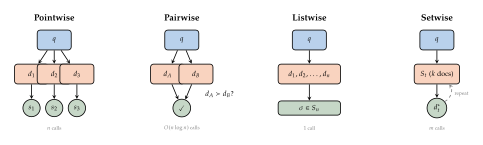
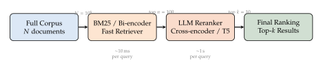
Empirical Comparison
Table 9 summarises the performance and efficiency characteristics of the major reranking approaches on the TREC Deep Learning benchmarks.
| Method | Paradigm | NDCG@10 | MRR@10 | LLM Calls |
| BM25 (no reranking) | – | 0.480 | 0.660 | 0 |
| BERT cross-encoder | Pointwise | 0.710 | 0.835 | 100 |
| monoT5 (3B) | Pointwise | 0.725 | 0.850 | 100 |
| duoT5 (3B) | Pairwise | 0.740 | 0.860 | 660 |
| LLM listwise (GPT-4) | Listwise | 0.750 | 0.870 | 5–10 |
| Setwise () | Setwise | 0.738 | 0.855 | 10 |
| FIRST | Listwise | 0.735 | 0.852 | 5–10 |
| RLCF-tuned | Listwise | 0.755 | 0.875 | 5–10 |
Insight.
The Accuracy-Efficiency Pareto Frontier No single reranking paradigm dominates all others. Pointwise methods are simple and parallelisable but leave quality on the table. Pairwise methods capture fine-grained preferences but are expensive. Listwise methods are the most accurate but limited by context length. Setwise methods offer the best balance for practical deployment. The optimal choice depends on the specific latency budget, the available model size, and the acceptable quality threshold. As a rule of thumb: if you can afford one LLM call per query, use listwise; if you need sub-second latency, use pointwise with a small cross-encoder; if you are somewhere in between, setwise with is a strong default.
Caution.
Do Not Trust a Single Reranker Blindly LLM rerankers can be confidently wrong. A reranker might assign high relevance to a document that matches the query's surface keywords but contradicts its intent, or demote a highly relevant document that uses different terminology. In high-stakes applications (medical, legal, financial), always combine the reranker's output with other signals (term matching, citation analysis, domain-specific knowledge graphs) and present multiple candidates to the user rather than relying on a single top-ranked result. The reranker is a powerful tool, but it is not an oracle.
Exercise 44.
Implement a monoT5-style pointwise reranker using a pre-trained T5-small model. Evaluate it on the MS MARCO passage ranking development set. Then implement the setwise variant with and . Compare NDCG@10 and wall-clock time per query.
Exercise 45.
Implement the sliding window listwise reranking algorithm from Algorithm 9. Experiment with different window sizes and step sizes . How many passes are needed for the ranking to converge? Plot NDCG@10 as a function of the number of LLM calls.
Synthetic Data Generation for Retrieval
Training a neural retriever requires labelled data: pairs of queries and relevant documents, annotated by human judges. But human annotation is expensive, slow, and often inconsistent. The TREC Deep Learning track, one of the most widely used benchmarks in information retrieval, contains only a few thousand judged queries. The MS MARCO dataset, substantially larger, still represents a tiny fraction of the possible query-document pairs. And when you want to deploy a retriever in a new domain, medical literature, legal documents, internal corporate knowledge bases, the training data simply does not exist.
This is the bootstrapping problem: building a retriever for a new domain requires training data, but obtaining that training data requires either a retriever (to surface documents for annotation) or an enormous human labelling effort. The solution, it turns out, is to let the language models generate the training data themselves.
InPars: Query Generation for Domain Adaptation
Bonifacio et al. [88] proposed InPars (Inquisitive Parrots), a method that uses large language models to generate synthetic queries for documents in a target corpus. The procedure is elegant in its simplicity.
Given a document from the target corpus, prompt the LLM with a few examples of (document, query) pairs drawn from a seed dataset, followed by the target document. The LLM then generates a plausible query for which would be a relevant answer. The synthetic query-document pair becomes a positive training example for the retriever.
Definition 50 (Few-Shot Query Generation).
Given a target document and a set of seed examples , the few-shot query generation procedure constructs the prompt: (Inpars Prompt) and samples from the language model. The resulting pair is added to the synthetic training set.
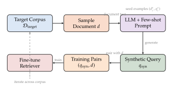
The synthetic training set is typically filtered to remove low-quality queries (e.g., those that are too short, too generic, or obviously unrelated to the document). A common filtering strategy uses the language model's own confidence: queries with low generation probability are discarded. The filtered set is then used to fine-tune a bi-encoder or cross-encoder retriever.
Example 34 (Domain Adaptation with InPars).
Consider adapting a general-purpose retriever to a biomedical corpus. The seed examples might include pairs from MS MARCO, such as:
Document: “Aspirin inhibits the enzyme cyclooxygenase”
Query: “How does aspirin work?”
Given a new biomedical document about the CRISPR-Cas9 mechanism, the LLM might generate the synthetic query “What is the mechanism of CRISPR-Cas9 gene editing?” This pair becomes training data for the domain-specific retriever, enabling it to handle biomedical queries without any biomedical annotations.
Remark 41.
The InPars procedure scales naturally with corpus size. For a corpus of documents, the cost is approximately LLM inference calls (one per document), each producing a short query. This is a one-time cost, amortised over the lifetime of the retriever. For a corpus of one million documents using a moderately sized LLM, the total cost is on the order of tens of dollars in API fees, a trivial expense compared to the cost of human annotation, which at $0.50 per query-document judgment would cost $500,000 for the same coverage.
Proposition 24 (Quality of InPars-Generated Training Data).
Let be a synthetic training set generated by InPars, and let be a retriever trained on . If the LLM's query generation distribution satisfies (Inpars KL) for all , where is the true distribution of user queries for which is relevant, then the retrieval performance gap satisfies: (Inpars Bound) where is the retriever trained on real human-annotated data.
Proof.
By Pinsker's inequality, the total variation distance between and is bounded by . The retriever's loss function (e.g., contrastive loss) evaluated under the synthetic distribution differs from its evaluation under the real distribution by at most the total variation distance times the maximum loss value. Since NDCG is bounded in , the gap in expected NDCG is bounded by . The bound follows by noting that the retriever optimised under the synthetic distribution is at most -suboptimal relative to the retriever optimised under the real distribution.
HyDE: Hypothetical Document Embeddings
If InPars generates synthetic queries for documents, HyDE (Hypothetical Document Embeddings) [89] does something conceptually reversed and strikingly beautiful: it generates synthetic documents for queries.
The core observation is this: queries and documents live in different linguistic spaces. A query is typically short, fragmentary, and ambiguous (“best treatment for lower back pain”). A relevant document is typically long, detailed, and self-contained (“Lumbar disc herniation is treated through a combination of physical therapy, anti-inflammatory medications, and in severe cases, surgical intervention”). Embedding a query and embedding a relevant document into the same space is precisely the challenge that makes dense retrieval hard.
HyDE bypasses this challenge entirely. Instead of embedding the query directly, it first uses an LLM to generate a hypothetical document: a passage that would plausibly answer the query. This hypothetical document, though potentially inaccurate in its specifics, captures the linguistic style, vocabulary, and topical focus of a relevant document. It is then embedded using a standard dense encoder, and the resulting embedding is used to retrieve real documents via nearest-neighbour search.
Definition 51 (Hypothetical Document Embedding).
Let be a generative language model and be a dense document encoder. The hypothetical document embedding for a query is: (HYDE) where is a hypothetical document generated by the language model in response to the query . Retrieval is then performed by finding the nearest neighbours of in the document embedding space: (HYDE Retrieval)
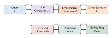
The beauty of HyDE is that it achieves zero-shot dense retrieval: it requires no training data whatsoever. The language model provides the domain knowledge (it knows what a relevant document would look like), and the dense encoder provides the embedding space (it maps the hypothetical document to the right neighbourhood in vector space). Neither component needs task-specific fine-tuning.
Algorithm 11 (HyDE Retrieval).
- Input: Query ; LLM generator ; dense encoder ; document index with pre-computed embeddings ; number of hypothetical documents ; number of results
- Output: Top- retrieved documents
- for
- generate hypothetical document
- encode hypothetical document
- average embeddings
- return
Key Idea.
Bridging the Query-Document Gap The fundamental challenge of dense retrieval is that queries and documents are linguistically different. A query asks a question; a document states facts. HyDE bridges this gap by transforming the query into the language of documents before embedding. The hypothetical document need not be factually accurate; it merely needs to be in the right region of the document embedding space. Even a hallucinated document about the right topic, using the right vocabulary, will embed close to real relevant documents.
Remark 42.
Generating multiple hypothetical documents () and averaging their embeddings improves robustness. Different generations may emphasise different aspects of the query, and averaging smooths out individual hallucinations while preserving the common topical signal. This is reminiscent of ensemble methods in supervised learning, where averaging predictions from multiple models reduces variance.
Example 35 (HyDE for Technical Queries).
Consider the query “Explain the attention mechanism in Transformers.” HyDE prompts the LLM to generate a hypothetical answer, which might read: “The attention mechanism in Transformers computes a weighted sum of value vectors, where the weights are determined by the compatibility between query and key vectors using a scaled dot-product” This hypothetical passage, though generic, occupies the same embedding neighbourhood as actual technical documents about Transformer attention. Dense retrieval using surfaces papers and tutorials about attention mechanisms, even though the original query is just a short imperative sentence.
Proposition 25 (HyDE Approximation Quality).
Let be the true relevant document for query , and let be the hypothetical document generated by the LLM. If the dense encoder is -Lipschitz (i.e., for a suitable text distance metric ), then: (HYDE Bound) In words, the distance between the HyDE embedding and the true document's embedding is bounded by the “textual distance” between the hypothetical and true documents, scaled by the encoder's Lipschitz constant. When the LLM generates a hypothetical document that is topically similar to (small ), the HyDE embedding lands close to the true document in the vector space, enabling successful retrieval.
Proof.
By the Lipschitz property of : which is the claimed bound. The bound is tight when the encoder preserves distances exactly (an isometry), and loose when the encoder collapses textual variations (as desired for robust retrieval).
Remark 43.
HyDE can fail in two characteristic ways. First, when the LLM generates a hypothetical document about the wrong topic entirely (a major hallucination), the HyDE embedding lands in a distant region of the vector space, and the retrieved documents are irrelevant. Second, when the query is highly specific and the LLM generates a generic answer, the HyDE embedding may be close to many documents but not specifically close to the one truly relevant document. The multi-sample averaging technique (Remark 42) mitigates the first failure mode but not the second. For highly specific queries, a traditional dense retriever trained on in-domain data typically outperforms HyDE.
Insight.
When to Use HyDE vs. Fine-Tuned Retrieval HyDE excels in zero-shot and low-resource settings where no task-specific training data is available. Its strength is precisely that it requires no training: plug in any LLM and any pre-trained encoder, and you have a working retriever. However, once labelled data becomes available (even synthetic data from InPars), a fine-tuned bi-encoder or cross-encoder typically surpasses HyDE, because fine-tuning directly optimises the query-document matching function. The practical recommendation is: use HyDE as a strong zero-shot baseline and a rapid prototyping tool, then transition to a fine-tuned retriever as training data accumulates. In the intermediate regime, where some data is available but not enough for reliable fine-tuning, HyDE can be combined with supervised signals by using the HyDE embedding as an additional feature in a learned scoring function.
Example 36 (HyDE Across Languages).
HyDE is particularly effective for cross-lingual retrieval, where the query is in one language and the documents are in another. A user issues a query in English: “What are the environmental effects of deforestation in the Amazon?” An LLM generates a hypothetical document in Portuguese (the language of many Amazon-related documents): “O desmatamento na Amazônia tem efeitos ambientais graves, incluindo perda de biodiversidade, alterações climáticas regionais” The multilingual encoder embeds this Portuguese hypothetical document close to real Portuguese documents about Amazonian deforestation. The approach requires no parallel corpora or cross-lingual training data; the LLM's multilingual capabilities handle the language transfer, and the multilingual encoder handles the embedding alignment.
Promptagator: Few-Shot Retriever Training
Promptagator extends the InPars idea by incorporating a consistency-based filtering step. After generating synthetic queries, a retriever is trained on the synthetic data and used to re-retrieve documents for each synthetic query. If the original document is not retrieved in the top- results for its synthetic query , the pair is considered unreliable and discarded. This round-trip consistency filter significantly improves the quality of the training data.
Definition 52 (Round-Trip Consistency Filter).
Given a synthetic training pair and a retriever trained on the current synthetic dataset, the round-trip consistency filter retains the pair if and only if: (Round TRIP) where denotes the documents with the highest retrieval scores for query .
The filtering is performed iteratively: generate synthetic data, train a retriever, filter the data using the trained retriever, retrain on the filtered data. Each iteration produces a cleaner training set and a stronger retriever.
Example 37 (Promptagator for Scientific Literature).
Suppose we wish to build a retriever for a corpus of 500,000 computer science papers. Promptagator proceeds as follows. First, generate synthetic queries for each paper using an LLM with 3 seed examples drawn from a small set of manually annotated queries. Second, train an initial bi-encoder on the resulting 500,000 synthetic pairs. Third, for each synthetic query , use the trained bi-encoder to retrieve the top-100 papers. If the original paper does not appear in this top-100 list, discard the pair as unreliable. Typically, 30–50% of pairs are filtered out in this step. Fourth, retrain the bi-encoder on the filtered dataset. The resulting retriever substantially outperforms the initial model, because the filtered pairs are those for which the query-document association is strong enough to survive a round-trip through the embedding space.
Synthetic Hard Negatives
Training effective retrievers requires not only positive examples (relevant documents) but also informative negative examples (irrelevant documents that are hard to distinguish from relevant ones). Random negatives are easy to obtain but provide little training signal; the model quickly learns to reject obviously irrelevant documents and stops improving. Hard negatives, documents that are topically related but not truly relevant, force the model to make fine-grained distinctions.
Language models can generate synthetic hard negatives by modifying relevant documents in subtle ways: changing key facts, altering the time period, or shifting the focus slightly. For a query about “treatment options for Type 2 diabetes,” a synthetic hard negative might discuss treatment options for Type 1 diabetes, or discuss Type 2 diabetes diagnostics rather than treatment.
Remark 44.
The difficulty of synthetic hard negatives must be carefully calibrated. Negatives that are too similar to positives may actually be relevant, introducing label noise. Negatives that are too dissimilar provide no training signal. A useful heuristic is to generate negatives that differ from the positive document in exactly one factual dimension while remaining topically coherent.
Risks and Limitations
Synthetic data generation for retrieval is powerful but fraught with risks. Three deserve particular attention.
Hallucination propagation.
When an LLM generates a synthetic query or document, it may hallucinate details that do not appear in the source document. If the retriever is trained to match these hallucinated details, it learns to retrieve documents based on fabricated content. This is particularly dangerous in high-stakes domains (medical, legal) where factual accuracy is paramount.
Distribution shift.
Synthetic data reflects the distribution of the language model, not the distribution of real user queries. LLM-generated queries tend to be more grammatical, more complete, and more informative than real user queries, which are often telegraphic, misspelled, and ambiguous. A retriever trained exclusively on synthetic data may underperform on real queries that fall outside the synthetic distribution.
Example 38 (Distribution Shift in E-Commerce Search).
An e-commerce company uses InPars to generate synthetic queries for its product catalogue. The LLM, trained on well-formed text, generates queries like “ergonomic office chair with lumbar support and adjustable armrests.” But real users type queries like “comfy desk chair” or “chair back hurt.” The retriever trained on synthetic data learns to match formal product descriptions to formal queries, but struggles with the colloquial, abbreviated, and sometimes ungrammatical queries that real customers actually submit. Mixing a small amount of real query logs into the training data mitigates this gap substantially.
Evaluation contamination.
This is perhaps the most insidious risk.
Caution.
The Evaluation Trap When synthetic data is generated from the same LLM that is used for evaluation, the resulting benchmarks may overestimate the retriever's true performance. The synthetic queries reflect the LLM's biases and knowledge, and a retriever trained on this data inherits those biases. If the evaluation queries are also LLM-generated, the retriever appears to perform well because it has learned to match the LLM's internal patterns, not because it genuinely understands relevance. Always evaluate on human-annotated benchmarks, ideally from a different distribution than the training data, and be sceptical of results that seem too good on synthetic evaluations.
Exercise 46.
Implement the InPars query generation pipeline for a domain of your choice. Use a pre-trained LLM to generate 10,000 synthetic queries for documents in your target corpus. Train a bi-encoder retriever on the synthetic data and evaluate on a held-out human-annotated test set. Compare against a retriever trained on MS MARCO data without domain adaptation.
Exercise 47.
Implement HyDE retrieval with hypothetical documents. Evaluate on three BEIR benchmark datasets. Does averaging more hypothetical documents consistently improve performance? How does the latency scale with ?
Exercise 48.
Design a controlled experiment to measure the effect of synthetic hard negatives on retriever quality. Train three versions of a bi-encoder: one with random negatives, one with BM25 hard negatives, and one with LLM-generated hard negatives. Compare Recall@100 and NDCG@10 on the TREC-DL 2020 test set.
Generative Retrieval
What if the search index is the model? Every retrieval system we have encountered so far maintains an external data structure, an inverted index, a vector store, a graph, to hold the corpus. The model (be it a sparse scorer, a dense encoder, or a cross-encoder) queries this external structure to find relevant documents. Generative retrieval eliminates the external index entirely. The model memorises the corpus in its parameters and, given a query, directly generates the identifier of the relevant document.
This is a radical departure from the retrieve-then-read paradigm. There is no index to build, no approximate nearest-neighbour search to perform, no document embeddings to store. The entire retrieval pipeline collapses into a single autoregressive generation step: query in, document identifier out.
The idea is audacious, elegant, and deeply controversial. Let us examine it carefully.
DSI: The Differentiable Search Index
Tay et al. [90] introduced the Differentiable Search Index (DSI), the seminal work in generative retrieval. The architecture is a standard sequence-to-sequence Transformer (T5) that is trained to perform two tasks:
Memorisation: given a document , generate its identifier . This phase forces the model to encode the content of every document in the corpus into its parameters.
Retrieval: given a query , generate the of the most relevant document. This phase teaches the model to map queries to the correct identifiers.
Definition 53 (Generative Retrieval Model).
A generative retrieval model is a parametric function that maps a query to a probability distribution over a set of document identifiers . Retrieval is performed by finding the identifier with the highest probability: (Generative Retrieval) When the identifier is a multi-token sequence , the probability factorises autoregressively: (Generative Autoregressive)
DocID Design
The design of the document identifier is the most critical architectural decision in generative retrieval. Tay et al. explored three approaches:
Numeric IDs.
Each document receives an arbitrary integer, represented as a sequence of digit tokens. Document 42,857 becomes the token sequence “4”, “2”, “8”, “5”, “7”. This is the simplest approach, but it forces the model to memorise an arbitrary mapping between document content and meaningless numbers, a task that is fundamentally at odds with the language model's strengths.
String IDs.
Each document receives a human-readable identifier, such as a title or URL. The document about tidal forces might receive the ID “Tidal_Force_Wikipedia”. This is more natural for the language model, since the identifier is semantically related to the content. However, titles may be ambiguous (multiple documents with similar titles) or too long to generate efficiently.
Semantic hierarchical IDs.
Documents are organised into a hierarchy via clustering, and each document's ID is its path through the hierarchy. For example, a corpus might be divided into 100 top-level clusters, each subdivided into 100 sub-clusters, and each sub-cluster containing individual documents. Document 42,857 might receive the hierarchical ID “37-15-42”, meaning cluster 37, sub-cluster 15, position 42. If the clustering is semantic (based on document embeddings), then similar documents have similar prefixes, and the model can learn to navigate the hierarchy by progressively narrowing the topic.
Key Idea.
Semantic Structure in Identifiers The key insight of hierarchical IDs is that they transform retrieval from a flat lookup problem into a structured navigation problem. Instead of predicting one of unrelated identifiers, the model predicts a sequence of tokens, each from a vocabulary of size . At each step, the model narrows the search space by a factor of , using the semantic content of the query to guide the descent through the hierarchy. This is analogous to traversing a B-tree in database systems, but learned end-to-end.
Training
DSI training proceeds in two phases. In the memorisation phase, the model is trained on input-output pairs of the form , where the input is the full document text (or a representative passage) and the output is the document identifier. The training objective is the standard sequence-to-sequence cross-entropy loss: (DSI Memorisation)
In the retrieval phase, the model is fine-tuned on query-document identifier pairs , where is a document known to be relevant to : (DSI Retrieval)
The total loss combines both phases: (DSI Total LOSS) where and are balancing coefficients.
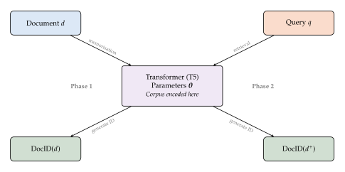
Example 39 (DSI on Natural Questions).
The original DSI experiments used the Natural Questions dataset, containing approximately 320,000 Wikipedia passages. With a T5-XXL backbone (11 billion parameters) and semantic hierarchical IDs, DSI achieved competitive recall with BM25 and dual-encoder baselines. The model effectively memorised the content of 320,000 passages and learned to route queries to the correct identifiers through the semantic hierarchy.
Remark 45.
At inference time, DSI uses beam search to generate document identifiers. With beam width , the model produces the top- most probable identifier sequences, which correspond to the documents that the model considers most relevant. This naturally supports top- retrieval: setting yields candidate documents. However, beam search can produce invalid identifiers (sequences that do not correspond to any document). Constrained beam search, which restricts each decoding step to tokens that are valid continuations of existing document IDs, eliminates this problem at a modest computational cost.
Lemma 8 (Constrained Decoding Preserves Ranking Quality).
Let be a prefix trie constructed from all valid document identifiers. Constrained decoding restricts the generation at each step to the set of valid continuations. The resulting ranking over valid identifiers is identical to the ranking obtained by unconstrained generation followed by filtering, i.e., for any two valid identifiers : (Constrained Ranking)
Proof.
Constrained decoding normalises the probability mass at each step over the valid continuation set: . Since the normalisation constant depends only on the prefix and not on the specific continuation , the relative ordering of continuations at each step is preserved. By induction over the sequence length , the relative ordering of complete identifiers is preserved.
Semantic IDs via Hierarchical Clustering
The design of meaningful document identifiers has emerged as a research direction in its own right. The most promising approach constructs identifiers through hierarchical clustering of document embeddings, producing IDs that reflect semantic structure.
RQ-VAE for Identifier Learning
Residual quantisation with a variational autoencoder (RQ-VAE) provides an elegant framework for learning semantic identifiers. The procedure works as follows:
Encode each document into a dense embedding .
Apply residual quantisation with levels. At level , find the nearest codeword in codebook : (Rqvae Quantise) where and is the residual after quantisation.
The semantic ID of document is the sequence of codebook indices: , where .
Definition 54 (Semantic Identifier via RQ-VAE).
A semantic identifier is a sequence of discrete codes obtained by applying residual quantisation to a document embedding. The identifier satisfies the property that semantically similar documents share common prefixes: (Semantic Prefix) where and are the semantic IDs of and respectively.
The connection to product quantisation, a well-established technique in approximate nearest-neighbour search, is direct. Product quantisation decomposes the embedding space into subspaces and quantises each subspace independently; residual quantisation applies quantisation sequentially to the residual error. Both produce compact codes that approximate the original embeddings, but residual quantisation produces naturally hierarchical codes: the first codeword captures coarse structure, and subsequent codewords refine it.
Proposition 26 (Reconstruction Error of RQ-VAE Semantic IDs).
After levels of residual quantisation with codewords per level, the reconstruction error for a document embedding is: (Rqvae Error) If the codewords are optimally placed (as in -means) and the embedding distribution is sub-Gaussian with variance proxy , then the expected reconstruction error satisfies: (Rqvae Bound) where is the embedding dimension, is the codebook size, and is a contraction factor that depends on the distribution's tail behaviour. Each additional level reduces the error geometrically.
Proof sketch.
At each level , the residual is the quantisation error of under the codebook . By the rate-distortion theory for -means quantisation of a -dimensional sub-Gaussian random vector, the expected distortion at each level is bounded by , where is the variance of . Since for optimal quantisation with contraction (approximately), the bound follows by induction.
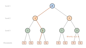
TIGER: Generative Retrieval for Recommendation
Rajput et al. [91] extended generative retrieval to the recommendation setting with TIGER (Transformer Index for GEnerative Recommenders). In recommendation, the “corpus” is a catalogue of items (products, movies, songs), and the “query” is a user's interaction history.
TIGER assigns each item a semantic ID learned via RQ-VAE on item content embeddings (e.g., text descriptions, images, or audio features). The recommendation model, a Transformer, takes the user's interaction history (a sequence of semantic IDs of previously consumed items) and autoregressively generates the semantic ID of the next item to recommend: (Tiger) where is the semantic ID of the next item.
Remark 46.
TIGER offers several advantages over traditional collaborative filtering and content-based recommendation. First, the semantic IDs capture item content, enabling zero-shot recommendation for new items that share semantic features with existing items (the cold-start problem). Second, the autoregressive generation naturally supports diverse recommendations: beam search over the semantic ID tree produces multiple candidate items from different branches of the hierarchy. Third, the entire system is end-to-end differentiable, allowing joint optimisation of the ID assignment and the recommendation model.
Example 40 (TIGER for Music Recommendation).
Consider a music streaming service with 10 million tracks. TIGER encodes each track using audio features (mel-spectrograms), textual metadata (title, artist, genre tags), and collaborative signals (co-listen patterns). RQ-VAE with levels and codewords per level produces semantic IDs capable of addressing billion unique items. A user who has recently listened to jazz fusion tracks receives a sequence of semantic IDs like (42, 17, 8, 195), (42, 18, 3, 77), (42, 17, 12, 201). The shared prefix (42, 17, ...) indicates that these tracks live in a similar region of the acoustic embedding space. The Transformer generates the next semantic ID autoregressively, predicting first the coarse cluster (42, indicating jazz), then the sub-cluster (17, indicating fusion), then finer refinements. Beam search at each level produces diverse recommendations spanning different corners of the jazz fusion space.
Remark 47.
The semantic ID framework naturally addresses the cold-start problem. A new item added to the catalogue receives a semantic ID based on its content features alone (no interaction history required). Because the ID reflects the item's semantic characteristics, the recommendation model can immediately incorporate it: a new jazz fusion track receives an ID with prefix (42, 17, ...) and is automatically considered alongside existing tracks in that region. Traditional collaborative filtering models, which rely entirely on interaction patterns, cannot recommend items with zero interactions.
IDGenRec: LLM-RecSys Alignment
Tan et al. [92] proposed IDGenRec, which addresses a key limitation of previous generative recommendation models: the identifiers were designed independently of the language model. IDGenRec aligns the identifier design with the LLM's tokeniser and pre-trained knowledge.
Instead of numeric or RQ-VAE-based codes, IDGenRec generates textual IDs that consist of semantically meaningful word tokens from the LLM's vocabulary. Each item receives a textual identifier that is both unique and descriptive, e.g., “vintage leather messenger bag” rather than “42-15-7”. The LLM can leverage its pre-trained understanding of these words to make recommendations without needing to learn arbitrary code mappings from scratch.
Definition 55 (Textual Item Identifier).
A textual item identifier is a sequence of tokens drawn from the LLM's vocabulary such that:
Uniqueness: for all .
Semantics: the tokens are semantically related to the item's content, so that is high.
Conciseness: the identifier is short enough for efficient generation, typically tokens.
Remark 48.
The alignment between identifier tokens and the LLM's pre-trained knowledge is crucial. When a model encounters the textual ID “vintage leather messenger bag,” its pre-trained representations immediately activate concepts related to leather goods, bags, and vintage aesthetics. This semantic priming reduces the amount of fine-tuning needed to learn the recommendation task, because the model already “understands” what the identifier refers to. In contrast, a numeric ID like “42-15-7” provides no such semantic priming, and the model must learn the entire mapping from scratch.
Example 41 (IDGenRec for Movie Recommendation).
Consider a movie recommendation system. Traditional approaches assign each movie an arbitrary integer ID (e.g., MovieLens ID 1 for Toy Story). IDGenRec instead assigns the textual identifier “animated family adventure Pixar 1995.” Given a user's history encoded as a sequence of such textual IDs, the LLM generates the next textual ID autoregressively. If the user's history includes “animated family adventure Pixar 1995” and “animated princess musical Disney 1991,” the model might generate “animated musical comedy Disney 1992,” which maps to Aladdin. The generation leverages the LLM's knowledge of movie attributes, years, and studios, enabling recommendations that go beyond simple collaborative filtering patterns.
CorpusLM: Unified Retrieval and Knowledge
Li et al. [93] proposed CorpusLM, a unified framework that trains a single language model to perform both generative retrieval and knowledge-intensive language tasks (question answering, fact verification, dialogue). The key observation is that retrieval and knowledge tasks share a common requirement: the model must internalise the corpus and produce relevant information on demand.
CorpusLM trains on a mixture of tasks:
Retrieval: query DocID, as in DSI.
Generation: query answer, using knowledge stored in the parameters.
Memorisation: document DocID, to maintain corpus coverage.
The multi-task training enables knowledge transfer: the retrieval task forces the model to organise its knowledge by document, while the generation task forces it to extract and synthesise information across documents.
The training objective combines all three tasks: (Corpuslm LOSS) where is the retrieval loss (cross-entropy over DocIDs given queries), is the generation loss (cross-entropy over answer tokens given queries), and is the memorisation loss (cross-entropy over DocIDs given documents). The balancing coefficients , , control the relative importance of each task.
Key Idea.
Retrieval as a Byproduct of Language Modelling CorpusLM embodies a provocative hypothesis: retrieval and generation are not separate capabilities but two aspects of the same underlying competence. A model that truly “understands” a document should be able both to retrieve it (given a query that it answers) and to generate its content (given a prompt that describes it). By training a single model on both tasks, CorpusLM encourages the development of unified representations that support both capabilities. Whether this unified approach can scale to web-scale corpora remains an open question, but the conceptual elegance is undeniable.
Example 42 (CorpusLM for Question Answering).
Given the question “Who invented the telephone?”, CorpusLM can respond in two modes. In retrieval mode, it generates the DocID of the Wikipedia article about Alexander Graham Bell. In generation mode, it directly produces the answer “Alexander Graham Bell is credited with inventing the telephone in 1876.” Both responses draw on the same parametric knowledge, but the retrieval mode additionally provides provenance (the specific document).
Limitations and Open Questions
Generative retrieval is intellectually compelling but faces fundamental challenges that temper its practical applicability.
Scalability.
A Transformer must memorise the entire corpus in its parameters. As the corpus grows, the model must grow proportionally to maintain retrieval quality. The original DSI experiments used 320,000 passages; web-scale corpora contain billions. Can a model with a fixed parameter count memorise billions of documents? Information theory suggests not.
Corpus updates.
Adding a new document to a traditional index takes milliseconds. Adding a new document to a generative retrieval model requires retraining or at minimum fine-tuning the entire model, a process that takes hours or days. For corpora that change frequently (news, social media, e-commerce), this is a severe limitation.
Hallucinated identifiers.
An autoregressive model can generate identifier sequences that do not correspond to any document in the corpus. With numeric IDs, the model might generate “42857” when no document has that ID. With semantic hierarchical IDs, the model might navigate to a leaf node that is empty. Constrained decoding can mitigate this problem by restricting generation to valid prefixes at each step (see Lemma 8), but it adds computational overhead and complexity.
Lack of explainability.
When a traditional retriever returns a document, the relevance signal is transparent: a BM25 score highlights matching terms, a dense retriever provides an embedding similarity, and a cross-encoder produces an interpretable relevance probability. When a generative retrieval model produces a DocID, the reasons for selection are opaque. The model navigated its parametric memory through a series of autoregressive token predictions, and there is no straightforward way to explain why this particular document was selected over others.
Open Problem 5.
Open Problems in Generative Retrieval Several fundamental questions remain open in generative retrieval. First, can incremental learning techniques (continual learning, parameter-efficient fine-tuning) enable efficient corpus updates without catastrophic forgetting of previously memorised documents? Second, can generative retrieval models provide calibrated confidence scores, so that the system knows when it is uncertain about a retrieval result? Third, is there a principled way to combine generative retrieval with external indices, perhaps using the generative model for “semantic routing” to a coarse document cluster and an external index for fine-grained retrieval within the cluster? These questions sit at the intersection of information retrieval, continual learning, and neural network theory, and their resolution will determine whether generative retrieval remains an intellectual curiosity or becomes a practical alternative to index-based systems.
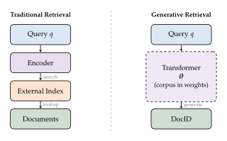
Theoretical Analysis
We now turn to the fundamental question: how many parameters does a generative retrieval model need to memorise a corpus of documents?
Proposition 27 (Memory Capacity for Generative Retrieval).
Let be a corpus of documents, each containing at most bits of information. A generative retrieval model that memorises the corpus with zero error requires at least parameters, where is the precision (number of bits) of each parameter.
Proof.
The corpus contains at most bits of information. Each parameter of the model stores at most bits (for a -bit floating-point representation). A model with parameters can store at most bits of information. For zero-error memorisation, we require , which gives .
More precisely, the model must store enough information to uniquely identify the relevant document for each possible query. If the mapping from queries to documents is injective (each query has a unique relevant document), then the model must distinguish outcomes, requiring at least bits per query. The total information stored must include both the document identifiers and the query-document associations, giving a lower bound of parameters.
Remark 49.
In practice, the required capacity is much larger than the information-theoretic lower bound. Neural networks are not optimal information storage devices: they store information in distributed representations with significant redundancy. Empirical observations suggest that a T5-XXL model (11B parameters, approximately 22 GB in 16-bit precision) can reliably memorise on the order of to passages. This is far below the capacity of a simple inverted index on the same hardware.
Conjecture 2 (Scaling Limit of Generative Retrieval).
A generative retrieval model can match the recall of an external-index retrieval system on a corpus of documents only when the model's parameter count scales at least linearly with . That is, there exists a constant (depending on the document distribution and query distribution) such that achieving Recall@ above a threshold requires parameters.
This conjecture, if true, implies that generative retrieval faces a fundamental scalability barrier. External-index systems scale sublinearly in compute (logarithmic for tree-based indices, constant for hash-based indices) and linearly in storage. If generative retrieval requires linear parameter scaling, then for sufficiently large corpora, the cost of the generative model will exceed the cost of maintaining an external index.
The evidence supporting this conjecture is both theoretical and empirical. On the theoretical side, Proposition 27 establishes that the parameter count must grow at least as , which is linear in for fixed document size . On the empirical side, published results show that generative retrieval quality degrades as corpus size grows beyond documents unless the model size is increased proportionally.
The Road Ahead
Generative retrieval represents a fascinating intellectual direction, but its practical impact remains uncertain. The approach excels in settings where the corpus is small, relatively static, and the model has ample capacity. For large-scale, dynamic corpora, external-index systems remain the pragmatic choice.
The most promising near-term application may be in hybrid systems that combine generative retrieval with traditional methods. A generative model can serve as one signal among many in a retrieve-then-rerank pipeline, contributing its unique ability to capture holistic query-document relationships that are difficult to express as sparse or dense similarity scores.
Historical Note.
From Memex to Generative Retrieval In 1945, Vannevar Bush described the Memex, a hypothetical device that would store all of a person's books, records, and communications, and allow them to be consulted with exceeding speed and flexibility. Bush envisioned a mechanical device with microfilm and levers. Eight decades later, generative retrieval attempts something remarkably similar: encoding an entire corpus in the weights of a neural network, consultable by natural language. The vision has come full circle, from mechanical storage to parametric memory, and the fundamental question remains the same: how do we organise human knowledge so that it can be retrieved when needed?
Exercise 49.
Implement a simplified DSI system using a pre-trained T5-small model and the Natural Questions dataset. Experiment with three types of DocIDs: random numeric, title-based string, and hierarchical (using -means clustering of document embeddings). Compare Recall@1 and Recall@10 for each ID type. Which ID strategy performs best, and why?
Exercise 50.
Implement semantic ID assignment using residual quantisation. Embed 10,000 Wikipedia passages using a pre-trained encoder, then apply RQ-VAE with levels and codewords per level. Visualise the resulting hierarchy: do semantically similar documents receive similar ID prefixes? Measure the collision rate (fraction of documents sharing an identical ID).
Exercise 51.
Design an experiment to empirically test the scaling conjecture (Conjecture 2). Train DSI models of increasing size (T5-small, T5-base, T5-large) on corpora of increasing size (, , passages). Plot Recall@10 as a function of the ratio (parameters per passage). Is there a threshold ratio below which performance collapses?
Exercise 52.
Implement a simplified TIGER-style recommendation system. Use the MovieLens 100K dataset. Assign semantic IDs to movies using RQ-VAE on movie plot embeddings (from a pre-trained sentence encoder) with levels and codewords per level. Train a small Transformer to predict the next movie's semantic ID given a user's viewing history. Compare Hit Rate@10 against a standard matrix factorisation baseline. Does the semantic ID structure help with cold-start recommendations for movies with few ratings?
Exercise 53.
Conduct a head-to-head comparison of generative retrieval (DSI with semantic hierarchical IDs) against dense retrieval (a bi-encoder with FAISS index) on the same corpus and query set. Measure three metrics: (1) Recall@10, (2) latency per query, and (3) memory footprint. At what corpus size does the external-index approach begin to dominate in each metric?
Retrieval-Augmented Generation – Foundations
Large language models are brilliant but forgetful. They can write sonnets, summarise legal briefs, and explain quantum mechanics to a five-year-old, yet they cannot reliably tell you who won last week's football match. They hallucinate references that do not exist. They confidently state facts that were true in 2021 but have since changed. They have no mechanism for updating their knowledge without expensive retraining. The root cause is architectural: all of the model's knowledge is compressed into its parameters during pre-training, and those parameters are frozen at inference time.
Retrieval-augmented generation (RAG) is the solution. The idea is disarmingly simple: give the language model a library card. Instead of requiring the model to memorise every fact it might ever need, equip it with a retrieval system that can look up relevant information at inference time and feed it into the generation process. The model still generates fluent language; it simply does so while consulting an external knowledge source.
This section traces the development of RAG from its original formulation [25] through modern extensions including RETRO [26], Fusion-in-Decoder [27], and Self-RAG [28]. We formalise the key architectures, analyse their training objectives, and examine the fundamental design decisions that determine when and how to retrieve.
The Original RAG Framework
The retrieval-augmented generation framework was introduced by Lewis et al. in 2020 [25]. The paper proposed a general-purpose architecture that combines a pre-trained retrieval module with a pre-trained sequence-to-sequence generator, training them jointly end-to-end.
Architecture
The RAG architecture comprises three components:
A parametric retriever , where is the input query and is a retrieved document. Lewis et al. used the Dense Passage Retriever (DPR), which encodes both queries and documents into dense vectors and retrieves by maximum inner product search: (DPR Score) where and are BERT-based encoders for queries and documents respectively.
A parametric generator , instantiated as a BART model that takes as input the concatenation of the query and the retrieved document , and generates an output sequence autoregressively.
A non-parametric knowledge index , a dense index over a large corpus (e.g., Wikipedia) that supports fast approximate nearest-neighbour search using MIPS (Maximum Inner Product Search).
The elegance of this design is the separation of concerns. The retriever is responsible for finding relevant information; the generator is responsible for using it. The knowledge index serves as a non-parametric memory that can be updated without retraining: to incorporate new information, one simply adds new documents to the index.
Definition 56 (Retrieval-Augmented Generation).
A retrieval-augmented generation (RAG) system is a tuple comprising:
A retriever parameterised by that maps an input to a distribution over documents from a corpus .
A generator parameterised by that produces output tokens conditioned on both the input and retrieved documents: .
A knowledge index of documents, each represented by a dense vector for efficient retrieval.
The joint probability of generating output given input is obtained by marginalising over retrieved documents: (RAG Marginal)
RAG-Sequence vs. RAG-Token
Lewis et al. proposed two variants that differ in how the marginalisation over retrieved documents is performed.
RAG-Sequence.
In RAG-Sequence, a single document is retrieved per output sequence. The model generates the entire output conditioned on that one document, and the final probability is a mixture over the top- retrieved documents: (RAG Sequence) Each document provides a coherent context for the entire generation. This is appropriate when the answer can be found in a single passage.
RAG-Token.
In RAG-Token, the marginalisation occurs at every output token. Different tokens in the output sequence can attend to different retrieved documents: (RAG Token) This is more expressive: the model can synthesise information from multiple documents within a single output, drawing one fact from document and another from . However, it requires forward passes through the generator at each token position, making it more expensive.
Remark 50.
The distinction between RAG-Sequence and RAG-Token mirrors a recurring theme in probabilistic modelling: where to place the summation over latent variables. In RAG-Sequence, the latent variable has global scope (one draw per sequence). In RAG-Token, it has local scope (one draw per token). The global variant is cheaper but less expressive; the local variant is richer but more computationally demanding. This is precisely analogous to the difference between a mixture model with a single latent assignment and a hidden Markov model with per-step latent states.
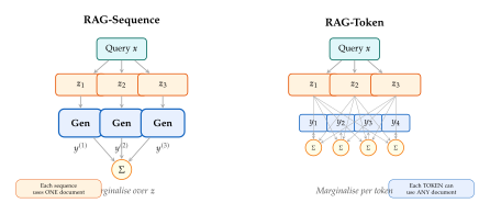
End-to-End Training
A distinctive feature of the original RAG framework is that the retriever and generator are trained jointly. The training objective maximises the marginal log-likelihood of the output given the input: (RAG Training)
The gradient flows through both the generator and the retriever. The generator learns which parts of the retrieved document are useful; the retriever learns which documents lead to correct outputs. This creates a virtuous cycle: better retrieval leads to better generation, which provides better training signal for retrieval.
In practice, the document encoder in the retriever is kept frozen during training (updating it would require re-indexing the entire corpus at each training step), while the query encoder and the generator are updated. This asymmetric update strategy is a pragmatic compromise: the query encoder learns to produce queries that match the document representations in the existing index.
Key Idea.
RAG Separates What the Model Knows from What It Can Access The fundamental insight of RAG is the separation between parametric knowledge (facts compressed into the model's weights during pre-training) and non-parametric knowledge (facts stored in an external index that can be queried at inference time). Parametric knowledge is fast to access but expensive to update and prone to staleness. Non-parametric knowledge requires a retrieval step but can be updated instantly by modifying the index. RAG gives the model the best of both worlds: the fluency and reasoning ability of a large language model combined with the currency and verifiability of an external knowledge store.
Algorithm 12 (RAG-Sequence Inference).
- Input: Query ; retriever ; generator ; knowledge index ; number of documents
- Output: Generated output
- Retrieve: Compute query embedding
- Find top- documents:
- Compute retrieval scores: for each
- Normalise: Retrieval probabilities
- for
- Generate: Beam search
- Compute generation log-prob:
- Marginalise:
- return
Example 43 (RAG for Open-Domain Question Answering).
Consider the question “What is the half-life of carbon-14?” The RAG pipeline proceeds as follows:
Encode query. The query encoder produces .
Retrieve. MIPS against the Wikipedia index returns the top-5 passages. The highest-scoring passage is from the article on radiocarbon dating: “Carbon-14 has a half-life of 5,730 40 years. It decays by beta emission to nitrogen-14”
Generate. The BART generator receives as input and produces “5,730 years.” The retrieval probability for is .
Marginalise. The model also generates answers conditioned on the other four passages. Passage (from an article on isotope geochemistry) also yields “5,730 years” with . The total probability mass on the correct answer is .
Output. The final answer is “5,730 years” with high confidence, directly grounded in retrieved evidence.
Without retrieval, the same BART model might produce “5,700 years” or even “5,000 years,” lacking the precision that only an external source can provide.
Historical Note.
From Information Retrieval to Neural Retrieval The marriage of retrieval and generation was not inevitable. For decades, information retrieval and natural language generation developed as separate fields with separate communities, separate conferences, and separate assumptions. Information retrieval, born in the library science tradition, focused on finding relevant documents from a collection. The dominant paradigms were term-frequency methods (TF-IDF, 1972), probabilistic models (BM25, 1994), and learning-to-rank approaches (2000s). Generation, by contrast, focused on producing fluent text, progressing from template-based systems to statistical models to neural sequence-to-sequence architectures.
The critical bridge was dense retrieval. When Karpukhin et al. introduced the Dense Passage Retriever (DPR) in 2020, they showed that a simple dual-encoder architecture trained on question-answer pairs could outperform BM25 on open-domain question answering. DPR made retrieval differentiable: the retrieval score was a smooth function of the query and document encoders, enabling end-to-end training through the retrieval step. Lewis et al. immediately exploited this by connecting DPR to BART, creating RAG. The insight was that if retrieval is differentiable, it can be treated as a latent variable and marginalised out during training, just like any other latent variable in a probabilistic model.
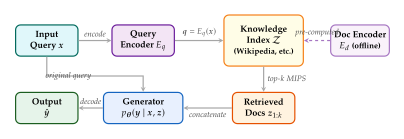
RETRO: Retrieval from Trillions of Tokens
The original RAG framework retrieves documents at the sequence level: given a query, retrieve passages and condition generation on them. RETRO (Retrieval-Enhanced Transformer), introduced by Borgeaud et al. [26], takes a fundamentally different approach. It retrieves at the chunk level, integrating retrieval directly into the transformer architecture at multiple points during generation.
Chunked Cross-Attention
The key architectural innovation in RETRO is chunked cross-attention (CCA). The input sequence is split into chunks of tokens each. For each chunk (the -th chunk of the input), RETRO retrieves the top- nearest neighbours from a database of 2 trillion tokens. These neighbours are then integrated into the model through a cross-attention mechanism that operates at specific layers.
Formally, let be the hidden states of chunk at layer , and let be the encoded representations of the retrieved neighbours for chunk , each of length . The chunked cross-attention computes: (Retro CCA) where are the standard query, key, and value projection matrices. The CCA output is added to the residual stream at designated “retrieval layers” (typically every third layer).
The critical advantage is efficiency. Because retrieval operates at the chunk level, the cross-attention cost scales with the chunk size rather than the full sequence length. Moreover, the retrieved neighbours are encoded by a frozen BERT encoder, avoiding the need to backpropagate through the retrieval index.
Lemma 9 (RETRO Chunked Cross-Attention Cost).
Let be the total input sequence length, the chunk size, the number of retrieved neighbours per chunk, and the length of each neighbour. The total cost of chunked cross-attention across all chunks is: (Retro CCA COST) This is linear in the sequence length , independent of the chunk size . In contrast, full self-attention over the input concatenated with all retrieved neighbours would cost , which is quadratic.
Proof.
There are chunks. For each chunk, the cross-attention computes queries from token representations and keys/values from neighbour representations, giving a cost of per chunk. Summing over all chunks: . The in the numerator and denominator cancel, yielding a cost that is independent of the chunk size.
Scaling Laws: Retrieval as a Substitute for Parameters
Perhaps the most striking finding from the RETRO paper is that retrieval can substitute for model parameters. A 7.5-billion-parameter RETRO model with access to a 2-trillion-token retrieval database achieves performance comparable to models with 25 times more parameters (around 175 billion, GPT-3 scale) without retrieval on language modelling benchmarks. This suggests a new dimension in the scaling laws for language models: instead of only scaling parameters and training data, one can also scale the retrieval database.
Proposition 28 (Retrieval-Parameter Trade-off).
Let denote the language modelling loss of a model with parameters, trained on tokens, with access to a retrieval database of tokens. Under the RETRO scaling regime, satisfies: (Retro Scaling) where are constants, are scaling exponents, and is the irreducible loss. The exponent for retrieval database size is positive, confirming that increasing the retrieval database reduces loss, even when and are held fixed.
Remark 51.
The practical implications of Proposition 28 are profound. Training a 25-billion-parameter model from scratch is enormously expensive, requiring thousands of GPU-hours. Indexing a 2-trillion-token database, by contrast, is a one-time cost that can be amortised across all queries. If retrieval can substitute for parameters at favourable exchange rates, then RAG is not just an accuracy improvement but an economic one: it reduces the total cost of achieving a given performance level.
Fusion-in-Decoder
Fusion-in-Decoder (FiD), proposed by Izacard and Grave [27], offers an elegant solution to a practical problem: how to condition generation on a large number of retrieved passages without the quadratic attention cost of concatenating them all into a single input sequence.
The key idea is simple but effective. Each retrieved passage is independently concatenated with the query and encoded by the encoder: (FID Encode) The encoded representations are then concatenated and fed to the decoder, which attends over all of them jointly: (FID Decode)
The advantage is computational. The encoder processes each passage independently, so its cost scales linearly with . Self-attention within each encoded passage is quadratic in the passage length, but since each passage is short (typically 100 tokens), the total encoder cost is where is the passage length. This is far cheaper than encoding a single concatenated sequence of length , which would cost .
Lemma 10 (Fusion-in-Decoder Attention Complexity).
Let be the number of retrieved passages, each of length , and let be the output length. The attention cost of Fusion-in-Decoder is : the first term is the cost of independently encoding passages, and the second term is the cost of the decoder cross-attending over the concatenated encoder outputs at each of decoder steps. In contrast, a naive concatenation approach has cost for the encoder alone.
Proof.
The encoder processes passages independently, each of length . Self-attention in each has cost , so the total encoder cost is . The decoder has steps, and at each step it cross-attends over all encoder outputs, contributing per step for a total of . Adding both terms gives . The naive approach encodes a single sequence of length , with self-attention cost . Since is typically 10–100, the FiD approach is significantly cheaper.
FiD achieves state-of-the-art results on open-domain QA benchmarks (Natural Questions, TriviaQA) by leveraging up to 100 retrieved passages, a number that would be infeasible with naive concatenation. The decoder learns to cross-attend selectively, focusing on the most relevant passages and ignoring irrelevant ones.
Adaptive Retrieval: Self-RAG
The systems described so far retrieve for every query. But retrieval is not always necessary. If you ask a language model “What is 2 + 2?” it does not need to consult Wikipedia. If you ask it to write a haiku about autumn, retrieval might actually hurt by introducing irrelevant context that distracts the generator. The question is: can the model learn when to retrieve?
Self-RAG, introduced by Asai et al. [28], answers this question affirmatively. The model is trained to generate special reflection tokens that control the retrieval process and evaluate the quality of the generated output.
Reflection Tokens
Self-RAG introduces four types of reflection tokens:
[Retrieve]: Should the model retrieve? Values:
yes,no,continue. The model generates this token before each segment. If the value isyes, retrieval is performed; ifno, the model generates from its parametric knowledge alone.[IsRel]: Is the retrieved passage relevant to the query? Values:
relevant,irrelevant. Generated after retrieval, this token filters out passages that the retriever selected but that the generator judges as unhelpful.[IsSup]: Is the generation supported by the retrieved passage? Values:
fully_supported,partially_supported,no_support. This token enforces faithfulness: the model must assess whether its own output is grounded in the evidence.[IsUse]: Is the overall response useful? Values: rating from 1 to 5. This final reflection token provides an overall quality judgement.
The self-critique mechanism is the defining feature of Self-RAG. Rather than blindly incorporating retrieved information, the model reflects on the quality of retrieval and generation at each step. This transforms the model from a passive consumer of retrieved information into an active critic of its own output.
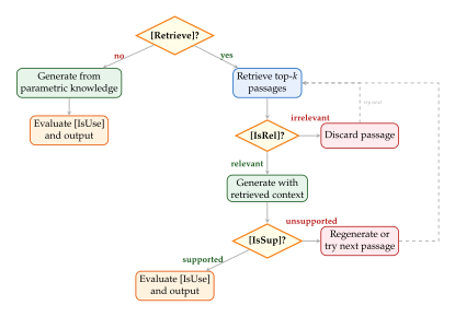
Training Self-RAG
Self-RAG is trained in two phases. First, a critic model is trained to generate reflection tokens given (query, passage, generation) triples. The critic is trained on data annotated by GPT-4, which labels each triple with the appropriate reflection token values. Second, the generator is trained to produce both the output text and the reflection tokens, using the critic's labels as supervision.
The training objective combines the standard language modelling loss with a reflection token prediction loss: (Selfrag LOSS) where [Retrieve], [IsRel], [IsSup], [IsUse] and is the cross-entropy loss for each reflection token. The hyperparameter controls the weight of the reflection loss.
Algorithm 13 (Self-RAG with Reflection Tokens).
- Input: Input ; generator ; retriever ; critique weights
- Output: Output with reflection scores
- Generate [Retrieve] token:
- if
- No retrieval needed
- Generate [IsUse]:
- return
- Retrieve:
- for
- Generate [IsRel]:
- if
- continue Skip irrelevant passages
- Generate output:
- Generate [IsSup]:
- Generate [IsUse]:
- Compute score:
- return
The Retrieve-Then-Read vs. Generate-Then-Retrieve Debate
The architectures discussed so far follow the retrieve-then-read paradigm: first retrieve relevant documents, then generate an output conditioned on them. An alternative paradigm inverts the order: generate-then-retrieve [94]. The model first generates a preliminary answer or a set of search queries, then retrieves documents to verify, refine, or extend the initial generation.
The generate-then-retrieve approach has several advantages. First, the model's initial generation can serve as a better query than the raw input, because the model can reformulate the question, expand acronyms, and resolve ambiguities. Second, the retrieved documents can serve as a verification mechanism: if the initial generation is consistent with the retrieved evidence, confidence increases; if it contradicts the evidence, the model can revise.
A formal comparison clarifies the trade-offs. Let be the input, the retriever, and the generator.
Retrieve-then-read.
(Retrieve THEN READ) The retrieval query is itself. If is ambiguous, under-specified, or uses different terminology than the documents in the index, retrieval may fail.
Generate-then-retrieve.
(Generate THEN Retrieve) The retrieval query is the model's preliminary generation , which may be more informative than the raw input. However, this requires two generator passes and one retrieval call, increasing latency.
Iterative retrieval-generation.
(Iterative RAG) The model iteratively refines its output, using each intermediate result as a retrieval query for the next round. This is the most expressive but also the most expensive approach, requiring generator passes and retrieval calls.
Remark 52.
The retrieve-then-read and generate-then-retrieve paradigms are not mutually exclusive. Modern systems increasingly adopt iterative approaches that alternate between generation and retrieval: generate an initial draft, retrieve supporting evidence, revise the draft, retrieve again if necessary, and so on. This iterative pattern mirrors how human experts write: draft, research, revise, repeat. The choice among these paradigms depends on the latency budget, the complexity of the query, and the quality of the initial retrieval. For simple factoid questions, retrieve-then-read suffices. For complex multi-hop reasoning, iterative approaches are often necessary.
Insight.
The Quality of the Retrieval Query Determines the Quality of the RAG Output A RAG system is only as good as its retrieval queries. If the query fails to capture the user's intent, the retrieved documents will be irrelevant, and the generator will either hallucinate or produce a generic answer. The generate-then-retrieve paradigm addresses this by using the model's own understanding of the query to formulate a better retrieval request. Self-RAG addresses it by allowing the model to assess retrieval quality after the fact and retry if necessary. Both approaches recognise the same fundamental truth: retrieval is not a solved problem, and the interface between the model and the index deserves as much attention as the model architecture itself.
Exercise 54.
Consider a factoid question answering task with 10 million documents in the index.
Write the RAG-Sequence and RAG-Token objectives for this setting. Under what conditions does RAG-Token reduce to RAG-Sequence?
A user asks: “What country has the largest population?” The model retrieves five passages, three of which mention India (with 2024 data) and two of which mention China (with 2020 data). Explain how RAG-Sequence and RAG-Token would handle this discrepancy differently.
Propose an extension of Self-RAG that generates not only reflection tokens but also re-query tokens that reformulate the retrieval query based on the initial results. Write pseudocode for your proposed algorithm.
Exercise 55.
Consider a RETRO model with chunk size , retrieved neighbours per chunk, and a retrieval database of tokens.
Derive the total number of cross-attention operations per input chunk, assuming neighbour length and hidden dimension .
If the retrieval database doubles from to , estimate the expected improvement in perplexity using the scaling law in (Retro Scaling), assuming .
Compare the memory footprint of storing tokens in a dense index (with -dimensional vectors in float16) vs. storing the same number of parameters in a transformer model. Which is more cost-effective?
RAG for Grounding and Verification
Large language models generate text that is fluent, grammatical, and often convincing. The problem is that fluency and truth are orthogonal properties. A model can produce a paragraph that reads beautifully and is entirely false. This is the hallucination problem, and it represents one of the most significant obstacles to deploying language models in high-stakes domains such as medicine, law, and finance.
Retrieval offers a path toward solving this problem. If every claim in the model's output can be traced to a specific source document, then the output is grounded: it is connected to verifiable evidence rather than floating free in the space of plausible-sounding text. This section examines how RAG enables grounding, how to evaluate it, and how to extend it to multi-step reasoning and formal verification.
Attribution and Faithfulness
Two related but distinct concepts govern the quality of grounded generation.
Definition 57 (Attribution).
A generated claim is attributed to a source document if contains information that, according to a reasonable reading, supports . Formally, let denote a natural language inference judgement. Then is attributed to if .
Definition 58 (Faithfulness).
A generated output consisting of claims is faithful to a set of retrieved documents if every claim is attributable: (Faithfulness)
Theorem 10 (Faithfulness Bound via Retrieval Quality).
Let be the top- retrieved passages for query , and let be the generated output. Let be the fraction of relevant passages in , and let be the probability that the generator produces a faithful claim given a relevant passage. Then the expected faithfulness score satisfies: (Faithfulness Bound) That is, faithfulness improves with both retrieval precision and the number of retrieved passages, approaching 1 as either , , or increases.
Proof.
A claim is faithful if at least one retrieved passage is both relevant and supports the claim. The probability that a single passage is relevant and supports is at least (precision times generator faithfulness given relevance). The probability that no passage supports is at most , assuming independence across passages. Therefore, . Since this holds for each claim, the expected faithfulness score (the average over claims) satisfies the same bound.
The distinction between attribution and faithfulness, on one hand, and correctness, on the other, is crucial. A claim can be faithfully attributed to a source and still be wrong, if the source itself contains an error. Attribution tells us where the information came from; it does not guarantee that the source is reliable.
Caution.
Attribution Is Not Verification A grounded claim can still be wrong if the source is wrong. Attribution establishes provenance, not truth. If a RAG system retrieves an outdated Wikipedia article stating that Pluto is a planet, and the generator faithfully reproduces this claim, the output is attributed (we can trace it to a source) and faithful (it accurately reflects the source) but incorrect (Pluto was reclassified in 2006). Verification requires an additional step: assessing the reliability and currency of the source itself. In high-stakes domains, RAG systems should not only retrieve and attribute but also rank sources by trustworthiness, recency, and authority.
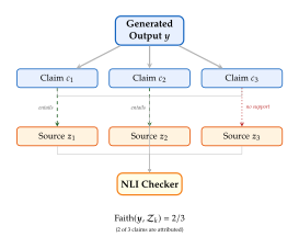
RAG Evaluation Frameworks
Evaluating a RAG system requires assessing multiple dimensions simultaneously. A system that retrieves relevant documents but generates unfaithful answers is dangerous. A system that generates faithful answers to the wrong question is useless. The community has developed multi-dimensional evaluation frameworks to capture these distinctions.
RAGAS: Retrieval-Augmented Generation Assessment
The RAGAS framework [95] decomposes RAG quality into three orthogonal dimensions:
Context relevance: Are the retrieved passages relevant to the query? This measures retrieval quality independently of generation. Let be the query and be the retrieved passages. Context relevance is: (Context Relevance)
Faithfulness: Does the generated answer accurately reflect the retrieved context? This measures whether the generator introduces information not supported by the retrieval. Let be the generated answer decomposed into claims . Faithfulness is: (Faithfulness Score)
Answer relevance: Does the generated answer actually address the query? A faithful answer to the wrong question scores high on faithfulness but low on answer relevance. Answer relevance is measured by generating synthetic questions from the answer and computing their semantic similarity to the original query: (Answer Relevance) where is the set of synthetic questions generated from and is a semantic similarity function.
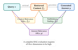
Retrieval-Specific Metrics
Beyond the RAGAS dimensions, several metrics target retrieval quality directly [96]:
Precision@: The fraction of top- retrieved passages that are relevant: (Precision AT K)
Recall@: The fraction of all relevant passages that appear in the top-: (Recall AT K)
Attribution accuracy: The fraction of generated claims for which the system can identify a supporting source passage. This differs from faithfulness in that attribution requires an explicit link between claim and source, not merely entailment.
Example 44 (Diagnosing RAG Failures with RAGAS).
Consider a medical QA system with the query: “What are the side effects of metformin?”
Scenario A: Low context relevance. The retriever returns passages about diabetes management in general, none of which specifically discuss metformin. . The generator hallucinates side effects from its parametric knowledge. (most claims are unsupported by retrieval). (the answer does address the question). Diagnosis: retriever failure.
Scenario B: High context relevance, low faithfulness. The retriever returns the correct passages. . But the generator introduces a claim that “metformin causes liver failure,” which none of the retrieved passages support (metformin is contraindicated in liver disease but does not cause it). . . Diagnosis: generator unfaithfulness.
Scenario C: High faithfulness, low answer relevance. The retriever returns relevant passages and the generator faithfully reproduces their content. But the passages discuss metformin's mechanism of action, not its side effects. (partially relevant). . . Diagnosis: the retriever found passages about the right drug but wrong topic.
Each scenario requires a different fix: improving the retriever (A), constraining the generator to be more faithful (B), or refining the retrieval query to match the question's intent more precisely (C).
Verification with Retrieved Facts
Grounding takes on special significance in formal domains where correctness can be mechanically checked. Consider theorem proving: a domain where every claim must be logically deduced from axioms and previously established results.
Theorem Proving with Retrieved Lemmas
A particularly compelling application of RAG is automated theorem proving, where the model generates proof steps and retrieves relevant lemmas from a mathematical library to support each step. This connects directly to the formal verification tools discussed in the evolutionary AI chapter, particularly the Lean theorem prover [97].
The proof verification pipeline operates as follows:
Conjecture. The system is given a mathematical statement to prove.
Generate candidate proof steps. A language model proposes a sequence of proof tactics, each of which transforms the current proof state.
Retrieve related theorems. For each proposed tactic, the system retrieves potentially relevant lemmas, definitions, and previously proven theorems from the mathematical library (e.g., Lean's
mathlib).Verify consistency. Each proof step is checked by the formal verifier (Lean's type checker) to ensure it is logically valid. Retrieved lemmas that the proof step depends on must themselves be verified theorems.
Iterate. If a step fails verification, the model backtracks and generates alternative steps, potentially with new retrieval queries informed by the failure.
This pipeline was spectacularly demonstrated by AlphaProof [98], which solved International Mathematical Olympiad problems by combining a language model with the Lean theorem prover. The retrieval component was essential: the model needed access to a vast library of mathematical facts to construct valid proofs.
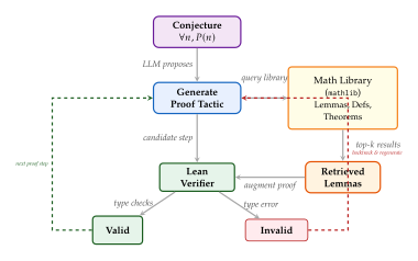
Example 45 (Retrieval-Augmented Proof Construction).
Suppose the goal is to prove that is irrational in Lean.
The model generates the initial tactic: “assume for contradiction
that with .” The retrieval
system queries mathlib and returns:
Nat.Coprime.eq_one_of_self_mul_self: if and , then .Int.sqrt_two_not_rat: a direct proof (which the model could invoke if available).Int.even_iff_two_dvd: is even iff .
The model uses the first and third lemmas to construct the classic infinite descent argument: implies is even, so , giving , which implies is even, contradicting . Each step is verified by Lean's type checker, ensuring logical correctness.
Exercise 56.
Consider building a retrieval-augmented theorem prover for a library containing 50,000 lemmas.
Each lemma statement is encoded as a 768-dimensional dense vector. Compute the memory required for the index in float32 and in float16. How does this compare to the memory footprint of a 7B-parameter language model?
The prover generates a proof tactic and needs to retrieve the 10 most relevant lemmas. If the inner product computation takes time per lemma, what is the total retrieval time? How could approximate nearest-neighbour methods (e.g., HNSW) reduce this?
Discuss the failure modes unique to retrieval-augmented theorem proving. How does retrieval failure (returning irrelevant lemmas) differ in its consequences from retrieval failure in open-domain QA?
Propose a method for the theorem prover to learn which lemmas are most useful for which types of proof goals, using the success or failure of the Lean verifier as a reward signal. How does this relate to reinforcement learning from human feedback (RLHF)?
Grounding in Multi-Step Reasoning
Many real-world queries require multi-step reasoning. The question “Did the architect of the Eiffel Tower also design the Statue of Liberty's internal structure?” requires the model to (1) identify the architect of the Eiffel Tower (Gustave Eiffel), (2) identify the designer of the Statue of Liberty's internal structure (also Gustave Eiffel), and (3) determine that they are the same person. Each step may require its own retrieval.
Two approaches have emerged for combining retrieval with chain-of-thought reasoning:
Retrieve once, reason many.
Retrieve all potentially relevant documents at the outset, then perform multi-step reasoning over the retrieved set. This is efficient (only one retrieval call) but may miss documents that become relevant only after intermediate reasoning steps.
Interleaved retrieval and generation.
Retrieve at each reasoning step, using the intermediate results to formulate new retrieval queries. This is more expressive: the model can discover that it needs information about Gustave Eiffel only after the first retrieval reveals him as the Eiffel Tower's architect.
Proposition 29 (Interleaved Retrieval Dominates Single Retrieval).
Let be a query requiring reasoning steps. Let be the set of documents retrieved by a single retrieval call on , and let be the union of documents retrieved at each reasoning step. Then in general does not hold (the two sets may be incomparable), but the information-theoretic utility satisfies: (Interleaved) where denotes mutual information and is the correct answer. Equality holds when all relevant information is retrievable from the original query alone.
Proof.
Define the sequence of reasoning states , where incorporates information from retrieval steps . At each step , the retrieval is conditioned on , which encodes the accumulated reasoning. By the data processing inequality, conditioning on more information cannot decrease mutual information: . The total information from interleaved retrieval is , which by the chain rule of mutual information and the fact that each is conditioned on the optimal state , is at least as large as the single-retrieval quantity.
Exercise 57.
Consider the multi-hop question: “What is the population of the country where the inventor of the telephone was born?”
Identify the reasoning steps required and the retrieval query appropriate for each step.
For the “retrieve once” approach, write a single query that might retrieve all necessary information. Analyse why this query is likely to fail.
Implement the interleaved approach as pseudocode, showing how each retrieval query is formulated based on the previous step's result.
Compute the number of retrieval calls for each approach and discuss the latency-accuracy trade-off.
RAG Across Modalities
The RAG paradigm was born in the world of text, but information does not respect modality boundaries. A doctor diagnosing a patient may need to retrieve medical images alongside journal articles. An engineer troubleshooting a machine may need to retrieve schematic diagrams, maintenance logs in text, and even audio recordings of the machine's operation. A student writing a report may need to retrieve figures, tables, and charts from papers.
Extending RAG to multiple modalities introduces new challenges. How do you index and retrieve images alongside text? How do you fuse information from a retrieved audio clip with a text prompt? What happens when the retrieval modality differs from the generation modality?
This section surveys multimodal RAG across vision, speech, audio, and video, tracing the rapid expansion of the RAG paradigm beyond its textual origins.
Visual Document RAG
Many real-world documents are not plain text. They contain tables, charts, diagrams, equations, and complex layouts that lose crucial information when converted to text via OCR. Visual document RAG addresses this by treating document pages as images and retrieving them based on visual similarity.
VDocRAG: Visually-Rich Document RAG
VDocRAG [29] operates on the principle that the visual rendering of a document is often more informative than its textual extraction. A table in a financial report, for instance, has a spatial structure (rows, columns, headers) that is immediately apparent from the visual rendering but is destroyed by naive text extraction.
The VDocRAG pipeline comprises:
Visual encoding. Each document page is encoded as an image by a vision encoder (e.g., a Vision Transformer), producing a dense representation for page image .
Visual indexing. The page representations are stored in a dense index, analogous to the text index in standard RAG but over visual representations.
Query-visual retrieval. Given a text query , a cross-modal encoder maps it to the same representation space: . Retrieval is by maximum inner product search: .
Visual-grounded generation. The retrieved page images are fed to a vision-language model that generates the answer conditioned on both the query and the visual content.
The advantage over text-based RAG is substantial for documents with rich visual structure. Tables, charts, and diagrams are retrieved and interpreted in their native visual form, avoiding the information loss inherent in OCR and layout parsing.
Multi-Level Visual QA
Not all visual information is at the same granularity. A question about a specific cell in a table requires fine-grained retrieval; a question about overall trends in a chart requires coarser retrieval. Multi-level VQA [99] addresses this by retrieving at multiple granularities simultaneously: document level, page level, region level, and element level.
Definition 59 (Multi-Level Retrieval).
A multi-level retrieval system maintains indices at granularity levels , where contains representations at granularity level (e.g., document, page, region, element). Given a query , the system retrieves at each level: for . The generator conditions on the union: (Multilevel)
Knowledge-Based Visual QA
Some visual questions require external knowledge that is not present in the image. The question “What architectural style is this building?” given a photo requires the model to recognise visual features (pointed arches, flying buttresses) and link them to knowledge about Gothic architecture. KB-VQA systems retrieve from a knowledge base (e.g., Wikipedia, Wikidata) conditioned on both the image and the question, fusing visual perception with encyclopaedic knowledge.
The KB-VQA pipeline combines three types of representation:
A visual representation capturing the image content.
A textual representation capturing the question semantics.
A knowledge representation capturing the retrieved facts from the knowledge base.
The generator fuses all three: . This three-way fusion is more complex than standard text RAG but enables answering questions that require both visual perception and world knowledge.
Example 46 (KB-VQA in Practice).
A user photographs a building and asks: “When was this building constructed?” The visual encoder recognises features consistent with Art Deco architecture (geometric forms, stepped facade, decorative spandrels). The cross-modal retriever queries a knowledge base and returns the Wikipedia article on the Empire State Building, which includes the construction date (1930–1931). The generator produces: “This building, which appears to be the Empire State Building based on its Art Deco features, was constructed between 1930 and 1931.” The answer integrates visual recognition, knowledge retrieval, and natural language generation.
Speech RAG
Speech processing introduces unique challenges for RAG. Audio signals are high-dimensional and temporally extended. Traditional speech systems rely on an ASR (automatic speech recognition) pipeline to transcribe audio to text, then apply text-based RAG. But this pipeline approach has a fundamental flaw: ASR errors propagate through the entire system. A misrecognised proper noun in the transcription leads to a failed retrieval, which leads to a wrong answer.
ReSLM: Retrieval-Enhanced Speech Language Model
ReSLM [30] addresses the domain adaptation problem in speech recognition through retrieval. When a speech model encounters domain-specific entities (medical terms, company names, technical jargon), it often fails because these entities are underrepresented in its training data.
ReSLM works by maintaining a retrieval index of domain-specific entities along with their audio representations. When the speech model encounters an ambiguous segment, it retrieves the most likely entity from the index and biases the recognition toward it.
The architecture comprises:
Speech encoder. Encodes the input audio into a sequence of frame-level representations .
Entity retriever. For each audio segment, queries a joint speech-text index of domain entities. The index contains both the text form (“metformin”) and a representative audio embedding of each entity.
Biased decoding. The retrieved entities bias the decoder's output distribution via shallow fusion: (Reslm BIAS) where is the set of retrieved entities and is a bias weight.
WavRAG: Audio-Native RAG
WavRAG [31] takes a more radical approach: it bypasses ASR entirely, performing retrieval directly in the audio domain.
Insight.
Bypassing ASR Eliminates Error Compounding In a traditional pipeline, an ASR error rate of 10% means that roughly 10% of the retrieval queries contain errors. If the retrieval system has its own 10% error rate on correct queries, the compounded error rate on queries with ASR mistakes is substantially higher: the retriever receives a garbled query and returns irrelevant results. WavRAG's direct audio retrieval avoids this compounding: the retrieval operates on the original audio signal, not on a potentially corrupted transcription. The total error is that of a single system rather than the product of two.
WavRAG represents both audio queries and audio documents as embeddings in a shared space, using a model trained with contrastive learning. The query is an audio segment; the index contains audio segments paired with their metadata. Retrieval is by standard nearest-neighbour search in the embedding space.
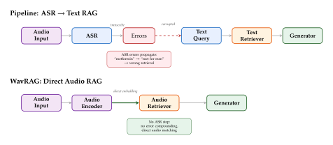
Audio RAG for Generation
The RAG paradigm extends naturally to audio generation. Just as a text RAG system retrieves passages to condition text generation, an audio RAG system retrieves audio clips to condition audio synthesis.
Re-AudioLDM: Retrieval-Augmented Audio Generation
Re-AudioLDM [32] augments a latent diffusion model for audio generation with a retrieval component based on CLAP (Contrastive Language-Audio Pretraining).
The system operates as follows:
Text prompt encoding. A text caption (e.g., “a dog barking in the rain”) is encoded by the CLAP text encoder into an embedding .
Audio retrieval. The CLAP embedding is used to retrieve the top- most similar audio clips from a large audio database: , where is the CLAP audio encoder.
Feature extraction. Acoustic features are extracted from the retrieved clips (e.g., mel-spectrograms, CLAP embeddings) and aggregated into a conditioning vector .
Conditioned diffusion. The latent diffusion model generates audio conditioned on both the text embedding and the retrieval features: (Reaudioldm) where is noise and is the denoised latent, which is decoded to a waveform by a vocoder.
The retrieved audio serves as an acoustic “reference” that guides the diffusion model toward realistic sound textures. Without retrieval, the model must generate the characteristics of rain, dog barking, and their interaction entirely from its parametric knowledge. With retrieval, it can copy acoustic textures from real recordings, producing outputs with greater fidelity and naturalness.
RECAP: Retrieval-Augmented Audio Captioning
The inverse task, describing audio in natural language, also benefits from retrieval. RECAP [33] retrieves similar audio clips along with their human-written captions and uses both the audio similarity and caption similarity to improve captioning quality.
The model computes a similarity-weighted aggregation of retrieved captions: (Recap) where is the query audio embedding, is the -th retrieved audio clip, is its caption, is a text encoder, and is a temperature parameter. This aggregated caption embedding conditions the captioning model, providing both semantic guidance (what sounds are present) and stylistic guidance (how to describe them).
Video RAG
Video introduces the temporal dimension to multimodal RAG. Retrieving relevant video clips for question answering requires understanding both the visual content and its temporal evolution. A question like “Show me the moment when the goal was scored” requires retrieving a specific temporal segment from a longer video.
Video RAG systems typically employ a two-stage approach. First, a video is segmented into clips (either by fixed temporal windows or by scene boundary detection). Each clip is encoded into a dense vector by a video encoder (e.g., a Video-Swin Transformer or a CLIP-based model). Second, at query time, the text query is encoded and matched against the clip representations. The retrieved clips condition the generation of the answer, which may be text (video QA), a temporal boundary (moment retrieval), or a summary (video captioning).
Formally, let be a video of frames. The video is partitioned into clips of frames each. Each clip is encoded as . At query time, the text query is encoded as , and the top- clips are retrieved: (Video RAG) The generator then produces the answer conditioned on the query and the retrieved clips: .
Remark 53.
Video RAG faces unique challenges compared to text or image RAG. The index is vastly larger (one hour of video at 30fps produces 108,000 frames), temporal alignment is critical (retrieving the right 3-second clip from a 2-hour video), and the modality gap between text queries and video content is wider than between text queries and text documents. Efficient indexing, hierarchical retrieval (first retrieve the right video, then the right clip, then the right frame), and strong cross-modal encoders are all essential.
Multimodal RAG Architecture
We now present a unified view of multimodal RAG, drawing together the modality-specific systems described above.
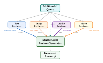
| System | Input | Output | Retrieval | Key Innovation |
| RAG [25] | Text | Text | DPR | End-to-end retriever-generator training |
| RETRO [26] | Text | Text | Chunk-level | Chunked cross-attention from trillion-token DB |
| FiD [27] | Text | Text | DPR | Independent passage encoding, joint decoding |
| Self-RAG [28] | Text | Text | Adaptive | Reflection tokens for when-to-retrieve |
| VDocRAG [29] | Text | Text | Visual | Retrieval over rendered document pages |
| ReSLM [30] | Speech | Text | Speech+Text | Entity-biased speech recognition |
| WavRAG [31] | Audio | Text | Audio | Direct audio retrieval, no ASR |
| Re-AudioLDM [32] | Text | Audio | CLAP | Retrieval-conditioned audio diffusion |
| RECAP [33] | Audio | Text | CLAP | Retrieval-augmented audio captioning |
Key Idea.
RAG Is a General Paradigm, Not a Text-Only Technique The RAG framework is modality-agnostic in its core design. The three components – a retriever, an index, and a generator – can be instantiated in any modality. What changes across modalities is the encoder (BERT for text, ViT for images, CLAP for audio, Video-Swin for video), the index structure (dense vectors, visual features, audio embeddings), and the generator (BART, diffusion model, speech synthesiser). The underlying principle remains the same: augment the generator's parametric knowledge with retrieved non-parametric information to improve accuracy, reduce hallucination, and enable adaptation to new domains without retraining.
Exercise 58.
Consider designing a RAG system for a museum guide application that must answer visitor questions about artworks using text descriptions, high-resolution images, and audio narrations.
Design the index structure. What representations would you store for each modality? How would you handle cross-modal retrieval (e.g., a text question about a painting)?
A visitor asks: “What technique did Monet use to paint the water in this painting?” Trace the multimodal RAG pipeline, specifying which modalities are retrieved and how they are fused.
Compare the pipeline approach (retrieve in each modality independently, then fuse) with a unified approach (encode all modalities into a shared space, retrieve jointly). What are the trade-offs in terms of index size, retrieval quality, and system complexity?
Extend the RAGAS evaluation framework to this multimodal setting. How would you measure context relevance when the context includes both an image and a text passage?
Exercise 59.
A hospital wants to deploy a speech-enabled RAG system for doctors who dictate patient notes and ask questions about drug interactions.
Explain why the pipeline approach (ASR text RAG) is particularly dangerous in this setting. Give a concrete example of how an ASR error could lead to a harmful outcome.
Design a WavRAG-style system for this application. Specify the audio encoder, the index contents (what audio clips and metadata to store), and the generation model.
The system must handle both English and Spanish speakers. How would you extend the retrieval index to support bilingual queries without maintaining separate indices for each language?
Compute the index size (in GB) for a database of 100,000 drug entities, each represented by a 512-dimensional float32 embedding, plus a 256-dimensional audio embedding. Is this feasible to deploy on a hospital server?
Open Problem 6.
Open Problems in Multimodal RAG Several fundamental challenges remain open in multimodal RAG:
Cross-modal alignment. Current systems use separately trained encoders for each modality. A unified encoder that produces aligned representations across text, image, audio, and video without modality-specific fine-tuning remains elusive.
Temporal retrieval. Retrieving the right moment from a long video or audio recording is far harder than retrieving a text passage. The temporal granularity problem (how long should a retrievable “chunk” be?) has no universal answer.
Evaluation. The RAGAS framework is designed for text. Extending faithfulness and attribution metrics to images (“is this generated description faithful to the retrieved image?”) and audio (“is this caption faithful to the retrieved audio clip?”) requires new evaluation paradigms.
Efficiency. Multimodal indices are orders of magnitude larger than text indices. One hour of video at 1fps produces 3,600 frame embeddings; a million hours produces 3.6 billion embeddings. Efficient indexing and approximate nearest-neighbour methods tailored to multimodal data are needed.
Memory-Augmented Retrieval
Every time you chat with a large language model, something remarkable happens: the model produces fluent, contextually appropriate responses that give the impression of understanding and recall. Yet the moment the context window ends, every detail of your conversation vanishes. The model does not remember your name, your preferences, or the intricate problem you spent forty minutes explaining. It wakes up, tabula rasa, with every new session.
This is not merely an engineering inconvenience. It is a fundamental limitation that separates current language models from anything resembling genuine intelligence. The solution is memory, and the central thesis of this section is that memory is retrieval. The two concepts are not merely analogous; they are computationally identical, differing only in the time scale over which information is stored and recalled.
The Memory-Retrieval Equivalence
The cognitive science of memory, from Tulving's seminal distinction between episodic and semantic memory [36] to Squire's taxonomy of memory systems [41], reveals a striking correspondence with the architecture of modern retrieval systems. Consider the three fundamental operations that any memory system must support:
Encoding. A new experience must be transformed into an internal representation suitable for storage. In the brain, this involves hippocampal pattern separation and the formation of engrams [34][35]. In a retrieval system, this is indexing: a document is embedded into a vector space and stored in an index.
Storage. The encoded representation must persist over time. Biological memory achieves this through synaptic consolidation, transferring fragile hippocampal traces into stable neocortical representations. A retrieval system achieves this through persistent vector databases, inverted indices, or key-value stores.
Retrieval. Given a cue (a thought, a sensation, a question), the system must recover the stored representation. In the brain, this is pattern completion: a partial cue activates the full memory trace. In a retrieval system, this is a query: the cue is embedded and the nearest neighbours in the index are returned.
Definition 60 (Memory-Augmented Retrieval System).
A memory-augmented retrieval system is a tuple where:
is an encoder that maps raw inputs (conversation turns, documents, experiences) to -dimensional embeddings,
is a memory store consisting of embedding-content-timestamp triples, where , is the raw content, and is the time of encoding,
is a retrieval function that, given a query embedding and the memory store, returns the top- most relevant memories,
is a decay function that periodically prunes or down-weights memories according to a forgetting policy.
The mapping between biological memory and retrieval is not merely metaphorical. It is structural: each component of Definition 60 has a direct neural counterpart.
Key Idea.
Memory is retrieval. They are the same computational problem operating at different time scales. Storing a memory is indexing a document. Recalling a memory is executing a retrieval query. Forgetting is index pruning with temporal decay. Once you see this equivalence, every advance in retrieval technology becomes an advance in artificial memory, and vice versa.
To make the equivalence precise, we define a relevance scoring function that combines the factors governing both biological recall and computational retrieval.
Definition 61 (Memory Relevance Score).
Given a query embedding , a memory , and the current time , the memory relevance score is (Relevance) where is a similarity function (e.g., cosine similarity), assigns an importance weight to each memory, and controls the rate of temporal decay.
This three-factor model captures a fundamental insight from psychology: we recall memories that are relevant to the current context (semantic similarity), that were important when they were formed (importance weighting), and that are recent (recency bias), unless their importance is sufficiently high to overcome the decay.
Example 47 (The Birthday Effect).
Consider a personal AI assistant that has been running for a year. A friend mentioned their birthday in passing eleven months ago ( months). With the decay parameter per month, the recency factor is . If the importance weight is low (), the memory will be difficult to retrieve. But if the assistant correctly classified the birthday as high-importance (), the effective score is , which may exceed the scores of more recent but less important memories. This mirrors human memory: you remember important events from long ago while forgetting trivial events from yesterday.
Remark 54.
The exponential decay in (Relevance) is motivated by Ebbinghaus's forgetting curve, one of the oldest quantitative laws in psychology. Ebbinghaus showed that retention decreases approximately exponentially with time, a finding that has been replicated thousands of times across different memory tasks and populations. The importance-weighted variant in our model corresponds to the well-documented effect of emotional salience on memory consolidation: emotionally significant memories are encoded more strongly and decay more slowly.
The Context Window Problem
The context window of a transformer-based language model is the maximum number of tokens it can attend to simultaneously. For GPT-4, this is 128K tokens. For Claude, it ranges up to 200K tokens. For Gemini 1.5 Pro, it is an impressive 1M tokens. These numbers sound large, but they are woefully insufficient for many real-world applications.
Consider a software engineer who wants an AI assistant to understand their entire codebase. A medium-sized project might contain 500,000 lines of code, or roughly 10 million tokens. Even Gemini's 1M-token context window can hold only 10% of this codebase. A lawyer reviewing discovery documents for a complex case may face millions of pages. A doctor's complete medical history may span decades of records. In every case, the context window is a bottleneck.
The fundamental issue is computational. Self-attention in a standard transformer has complexity in the sequence length . Doubling the context window quadruples the attention cost. Even with efficient attention variants (linear attention, FlashAttention, ring attention), the memory and compute costs of very long contexts remain substantial.
Proposition 30 (Context as Retrieval).
Let be a conversation history of turns, and let be the context window length of a language model. If , then any strategy for selecting which turns to include in the context window is equivalent to a retrieval problem: given the current query and the full history , select a subset with that maximises the model's performance on the current turn.
Proof.
The proof is essentially definitional, but the formalisation is instructive. Let be the language model with parameters and context window . The model's output at turn is for some subset of at most tokens. Let be a loss function measuring the quality of the model's output relative to the ideal next response . The optimal context selection strategy solves (Context OPT) This is precisely a retrieval problem: from the corpus , select the subset most relevant to the query (the current conversational context) subject to a budget constraint (the window length ).
Three main strategies have emerged for managing context when the conversation history exceeds the window:
Sliding Window.
The simplest approach: keep only the most recent tokens. This discards all information from earlier in the conversation. Formally, . The sliding window is cheap and simple but catastrophically forgetful: if the user mentioned a crucial constraint in the first message, it is gone forever once the window slides past it.
Summarisation.
Periodically compress older portions of the conversation into a summary. The context then contains the summary plus the recent turns: . Summarisation preserves more information than the sliding window, but the compression is lossy. Details are lost, nuances are flattened, and the quality of the summary itself depends on the model that generates it.
Retrieval-Augmented Context.
Store the entire conversation history in a retrieval index. At each turn, embed the current query and retrieve the most relevant past turns. The context becomes , where the last turns are always included for coherence and the retrieved turns provide relevant long-term context. This is the approach advocated by Definition 60: the conversation history is the corpus, each turn is a document, and the current query drives retrieval.
Example 48 (Comparing Context Strategies).
Suppose a user has a 200-turn conversation with a coding assistant (context window turns). In turn 5, the user specified: “All functions must return typed dictionaries, never raw tuples.” In turn 195, the user asks: “Write a function to parse the config file.”
Sliding window: The context contains turns 151–200. Turn 5 is lost. The assistant may return raw tuples.
Summarisation: If the summariser was good, the summary mentions the typing constraint. If not, it is lost.
Retrieval-augmented: When the query “Write a function to parse the config file” is embedded, the retrieval system can surface turn 5 because “typed dictionaries” and “function” have high semantic relevance to code-writing queries. The constraint is preserved.
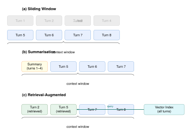
Memory-Augmented Architectures
The retrieval-augmented context strategy described above operates outside the model: the retrieval system selects context, and the model processes it as if it were ordinary input. A more ambitious approach integrates memory directly into the model architecture.
MemoryBank.
The MemoryBank framework [100] equips an LLM with a persistent external memory that is updated after each conversation. After each session, the system: (i) extracts key facts and events from the conversation, (ii) embeds them using the model's own encoder, (iii) stores them in a vector database with importance scores and timestamps, and (iv) applies the Ebbinghaus-inspired forgetting mechanism of (Relevance). At the start of each new session, the system retrieves relevant memories and injects them into the prompt.
Memorising Transformers.
The Memorising Transformer [101] takes a more architectural approach: it adds a NN-augmented attention layer that can attend to a large external memory of key-value pairs. During training, the model stores key-value pairs from previous batches in a memory bank. During inference, the attention mechanism computes attention scores over both the local context and the external memory: (MEM Transformer) where denotes concatenation, and are the keys and values from the current context, and and are retrieved from the external memory.
Connection to Engram Theory.
The concept of an engram, a physical trace of memory in the brain [34], provides a compelling biological parallel for memory-augmented architectures. In neuroscience, an engram is a specific pattern of neural activation that encodes a memory. Retrieval involves reactivating this pattern, which is precisely what a NN lookup over stored key-value pairs achieves. For a deeper treatment of memory architectures in neural networks, including their connection to continual learning, we refer the reader to our dedicated memory chapter (24).
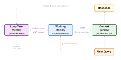
Retrieval for Continual Learning
The connection between memory and retrieval extends beyond conversation management to one of the deepest problems in machine learning: catastrophic forgetting. When a neural network is trained on a sequence of tasks, learning new tasks tends to overwrite the weights responsible for old tasks, causing performance on earlier tasks to collapse.
Retrieval offers an elegant solution. Rather than relying entirely on the network's parameters to encode all knowledge, we can store experiences (input-output pairs from previous tasks) in an external memory and retrieve them during training on new tasks. This is experience replay, one of the most effective strategies for continual learning (see 26 for a comprehensive treatment).
Proposition 31 (Retrieval Mitigates Catastrophic Forgetting).
Let be a model trained sequentially on tasks . Let be the loss on task . If at each training step on task , we retrieve examples from a memory buffer containing examples from tasks and include them in the training batch, then the expected increase in loss on any previous task satisfies (Forgetting Bound) where is a constant depending on the learning rate and the curvature of the loss landscape.
The bound reveals two key insights. First, the forgetting rate decreases as : more retrieved examples means less forgetting. Second, forgetting is worst when the gradients of the new task and the old task are highly conflicting (large gradient difference norm), which is precisely when replay is most needed.
The key design choice in retrieval-based continual learning is which experiences to store and retrieve. Random sampling works surprisingly well, but targeted strategies can do better:
Reservoir sampling maintains a uniform sample over all past experiences, regardless of which task they came from.
Herding-based selection chooses examples whose embeddings best approximate the mean embedding of each task, preserving the distributional properties of the original data.
Retrieval by gradient conflict: store examples whose gradients most conflict with the current task, since these are the ones most at risk of being forgotten.
Vector Embeddings for Memory
The practical implementation of memory-augmented retrieval hinges on the quality of the embeddings used to represent memories. A good memory embedding must satisfy several properties:
Semantic faithfulness. Semantically similar memories should have similar embeddings: should correlate with the semantic similarity of and .
Temporal awareness. The embedding should encode (or be accompanied by) temporal information, enabling recency-based retrieval.
Compositional structure. The embedding space should support operations like analogy (“what was the equivalent of in context ?”) and negation (“retrieve memories unlike ”).
Efficient indexing. The embeddings must be compatible with approximate nearest-neighbour data structures for fast retrieval.
In practice, conversation turns are typically embedded using the same encoder used for document retrieval (e.g., a sentence transformer or an API-based embedding model). The temporal component is handled separately, as in (Relevance), by storing timestamps alongside embeddings.
Algorithm 14 (Memory-Augmented Context Management).
Given a language model with context window , an encoder , a memory store , decay rate , importance function , and a new user query :
Encode query: .
Score memories: For each , compute .
Retrieve: Select the top- memories by score, where is chosen so that the total token count of plus the recent turns does not exceed .
Construct context: .
Generate: .
Store new memory: , where denotes concatenation.
Decay: Periodically remove memories where for a threshold .
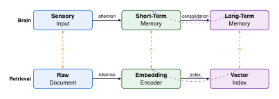
Historical Note.
The idea that memory and retrieval are fundamentally linked has deep roots. In 1972, Endel Tulving introduced the encoding specificity principle [36]: a memory can be retrieved only if the retrieval cue matches the conditions under which the memory was encoded. This is precisely the principle underlying embedding-based retrieval: a query retrieves a document only if their embeddings are similar, which happens only if they share semantic content. Tulving could not have known it, but his psychological principle anticipated the mathematical structure of modern vector retrieval by half a century.
Retrieval-Augmented Generation as Memory
With the memory-retrieval equivalence established, we can now view retrieval-augmented generation [25] through a completely new lens. A RAG system is not merely a clever engineering trick for injecting knowledge into a language model. It is a cognitive architecture: the language model is the “thinking” component (analogous to working memory and executive function), and the retrieval system is the “remembering” component (analogous to long-term memory).
Proposition 32 (RAG as Cognitive Architecture).
A RAG system consisting of a retrieval system and a language model is functionally equivalent to a memory-augmented cognitive system with:
Sensory buffer: the raw user query .
Working memory: the context window of , holding the query and retrieved documents.
Long-term memory: the retrieval index, containing all indexed documents.
Executive function: the model itself, which integrates information from working memory to produce a response.
Memory consolidation: the indexing pipeline that transforms raw documents into retrievable embeddings.
The system's behaviour is determined by the interaction between these components, just as human cognition arises from the interplay of working memory, long-term memory, and executive control.
This perspective immediately suggests improvements. If RAG is a cognitive architecture, then insights from cognitive science should transfer. For example:
Chunking: Cognitive science shows that working memory has limited capacity (the famous “7 2” items of Miller). Similarly, the context window has limited capacity. Just as humans chunk information to fit more into working memory, RAG systems should chunk retrieved documents into semantically coherent units rather than arbitrary token spans.
Spaced retrieval: In human memory, spaced repetition strengthens recall. In RAG, retrieving a document multiple times across different queries should increase its importance weight, making it more accessible in the future.
Interference: In human memory, similar memories interfere with each other (the fan effect). In retrieval, many similar documents in the index can reduce precision. De-duplication and diversity-promoting retrieval mitigate this.
The RETRO architecture [26] takes this cognitive perspective to its logical conclusion by interleaving retrieval directly into the transformer layers. At every chunk boundary, the model retrieves relevant passages from a massive external database and fuses them into the residual stream via cross-attention. The result is a model that “thinks and remembers” simultaneously, rather than treating retrieval as a separate pre-processing step.
Lemma 11 (Memory Capacity of RAG vs. Parametric Models).
Let be a parametric language model with parameters stored at -bit precision, and let be a retrieval system with access to a corpus of documents, each with entropy bits. The knowledge capacity of the parametric model is at most bits, while the knowledge capacity of the RAG system is at most bits. For typical values (, , , ), The retrieval component increases the effective knowledge capacity by nearly two orders of magnitude.
Exercise 60.
Consider a personal AI assistant with a memory store containing conversation turns spanning one year.
- (a)
If the decay parameter is per day and the importance weight is uniformly , what fraction of the oldest memories (from day 1) have a recency factor above 0.01?
- (b)
Propose an importance function that assigns higher weight to memories containing names, dates, and explicit user preferences. How would you implement this in practice?
- (c)
The user says “Remember, I am allergic to penicillin” on day 5. Argue that without a high importance weight, this critical memory might be irretrievable by day 300. Compute the minimum importance weight needed to keep the recency-weighted score above 0.1.
Exercise 61.
Prove that the memory-augmented context management algorithm (Algorithm 14) is optimal in the following sense: among all algorithms that select memories from based only on the relevance scores , the greedy top- selection maximises the sum of relevance scores in the retrieved set. Under what conditions might a non-greedy selection (e.g., diversity-promoting) yield better end-to-end generation quality despite a lower total relevance score?
Information-Theoretic Analysis of Retrieval
When you compress a 10,000-word document into a 3,072-dimensional vector embedding, how much information do you lose? And what are the consequences of that loss for retrieval accuracy?
These are not idle questions. Every retrieval system in production today, from Google Search to the RAG pipeline powering your favourite AI assistant, relies on a lossy compression step: documents are mapped to finite-dimensional vectors, and retrieval operates on these compressed representations rather than on the documents themselves. The information lost in this compression imposes a fundamental ceiling on retrieval accuracy, a ceiling that no amount of clever engineering can overcome.
In this section, we develop a rigorous information-theoretic framework for understanding this ceiling. We draw on Shannon's foundational work [4] and the modern theory of rate-distortion [37] to derive precise bounds on what embedding-based retrieval can and cannot achieve.
The Embedding as a Lossy Channel
Consider a document drawn from a source distribution over a document space . An embedding function maps to a -dimensional vector . From the perspective of information theory, the embedding function defines a channel from documents to embeddings, and the mutual information quantifies how much information about the document is preserved in the embedding.
The critical observation is that this channel is necessarily lossy: a real-valued vector in cannot, in general, encode all the information in an arbitrary document. The Data Processing Inequality provides the first constraint.
Theorem 11 (Data Processing Inequality for Retrieval).
Let be a document, its embedding, and the retrieved document. Then (DPI) where denotes mutual information and denotes entropy. Moreover, the first inequality is tight if and only if the retrieval function is a sufficient statistic of for .
Proof.
The documents, embeddings, and retrieved documents form a Markov chain: . By the Data Processing Inequality [37], for any Markov chain , we have . Applying this with , , gives the first inequality. The second follows from since mutual information cannot exceed the entropy of either variable. Equality in the first inequality holds if and only if is also a Markov chain, which is the condition for being a sufficient statistic.
Remark 55.
Theorem 11 tells us that every step in the retrieval pipeline can only destroy information, never create it. The embedding step loses information about the document. The indexing and approximate nearest-neighbour search lose information about the embedding. The re-ranking step may recover some information by consulting the original documents, but it cannot recover what was lost in the embedding. This is why the embedding quality is the single most important factor in retrieval system design.
Rate-Distortion Theory for Retrieval
Shannon's rate-distortion theory provides a precise framework for understanding the trade-off between compression and fidelity. We now apply it to the retrieval setting.
Let be a random document and its embedding. Define a distortion function that measures how much information relevant to retrieval is lost when is represented by . A natural choice is the retrieval distortion: (Distortion) which is 0 if the document is always in the top- results when relevant and 1 if it is never retrieved.
Definition 62 (Rate-Distortion Function for Retrieval).
The retrieval rate-distortion function is (Ratedistortion) where the minimisation is over all conditional distributions (i.e., all possible embedding functions, including stochastic ones) such that the expected retrieval distortion does not exceed .
The rate-distortion function tells us the minimum number of bits of mutual information needed between document and embedding to achieve a given level of retrieval accuracy. If we want distortion at most , we need at least bits of information in the embedding.
Theorem 12 (The Embedding Bottleneck).
For a -dimensional embedding with -bit precision per dimension (e.g., for float32), the maximum mutual information between document and embedding is bounded by (Bottleneck) Consequently, the minimum achievable retrieval distortion is bounded below by (MIN Distortion) where is the inverse of the rate-distortion function.
Proof.
The embedding is represented using floating-point numbers, each with bits of precision. The total number of distinct embeddings is at most . By the maximum-entropy principle, a discrete random variable taking at most values has entropy at most . Therefore bits, and since , the first bound follows.
For the second bound, observe that achieving distortion requires by the definition of the rate-distortion function. Since , we need , which gives since is a non-increasing function.
Example 49 (Capacity of a Modern Embedding).
Consider a state-of-the-art embedding model producing -dimensional vectors with float32 precision ( bits). The channel capacity is at most This is the theoretical maximum information content of the embedding. In practice, the actual mutual information is much lower because:
The embedding dimensions are correlated (reducing effective capacity).
The embedding function is not optimised for maximum mutual information but for contrastive similarity.
The float32 precision is not fully utilised: many embedding values cluster in a small range.
A realistic estimate might be 10–20% of the theoretical maximum, or roughly 10,000–20,000 bits. A typical English document of 5,000 words has an entropy of roughly 50,000–100,000 bits (at approximately 10–20 bits per word after accounting for linguistic redundancy). This means the embedding preserves at most 20–40% of the document's information. The rest is irrecoverably lost.
This is not a failure of any particular embedding model. It is a fundamental limit: you cannot losslessly compress 100,000 bits into 20,000 bits. The question is whether the embedding preserves the right 20%, namely the information most useful for retrieval.
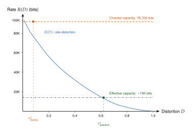
Insight.
The rate-distortion perspective reveals a sobering truth about embedding-based retrieval: there is a fundamental accuracy ceiling determined by the embedding dimension and precision. You can improve your embedding model, your training data, your loss function, and your approximate nearest-neighbour algorithm, but you cannot exceed the channel capacity of the embedding. The only way to raise the ceiling is to increase the embedding dimension, increase the precision, or move beyond pure embedding-based retrieval to hybrid approaches that consult the original documents (e.g., through re-ranking or multi-stage retrieval).
Information Loss in Embedding
The bottleneck theorem (Theorem 12) gives a worst-case bound based on the raw capacity of the embedding. We can obtain tighter bounds by reasoning about the structure of the information that embeddings capture and the information they discard.
Proposition 33 (Embedding Capacity Bounds Retrieval Recall).
Let be a corpus of documents, and let be an embedding function. For a query with a set of relevant documents , define recall@ as If the embedding has effective mutual information bits, and the documents are drawn i.i.d. from a distribution with entropy bits, then the expected recall@ is bounded by (Recall Bound)
Proof.
The embedding function partitions the document space into at most effectively distinguishable regions (by the operational meaning of mutual information as the logarithm of the effective alphabet size). Within each region, documents are indistinguishable by the retrieval system. Each region contains, on average, documents.
For a query with relevant documents, the top- retrieval can at best select the nearest regions and return all documents in them. The expected number of relevant documents retrieved is bounded by the sum of: (i) the relevant documents that fall in distinct regions (at most , weighted by ) and (ii) the chance alignment within shared regions. The factor accounts for the random baseline: even without any information, selecting out of documents uniformly at random yields relevant documents in expectation. The multiplicative boost from the embedding is at most , giving the stated bound.
Example 50 (Scaling Limits of Embedding Retrieval).
Consider a corpus of documents (roughly the scale of the indexed web). Suppose the effective mutual information is bits, and each query has relevant documents. With :
The bound gives , which is vacuous because is astronomically large. This tells us that for corpora of any practically conceivable size, the embedding capacity is not the binding constraint.
The constraint does bind when the effective information is very low. If bits (e.g., a very coarse binary hash), then , and each hash bucket contains about documents. Recall@10 would be approximately , or 1%. This quantifies the intuition that low-dimensional embeddings cannot support precise retrieval over large corpora.
The more practically relevant bound concerns the quality of information captured by the embedding, not just its quantity.
Theorem 13 (Retrieval Error from Irrelevant Information).
Decompose the document's information content as , where is the information lost in embedding. Further decompose the mutual information as (INFO Decomposition) where is the mutual information about features relevant to retrieval (e.g., topic, meaning, intent) and is mutual information about irrelevant features (e.g., formatting, writing style, document length). Then the effective retrieval capacity is (Effective Capacity) and the minimum retrieval distortion satisfies (Distortion Irrelevant) Every bit of embedding capacity wasted on irrelevant information is a bit unavailable for retrieval accuracy.
Proof.
The decomposition follows from the chain rule for mutual information applied to any partition of the document's features into relevant and irrelevant components. By Theorem 12, . Since , we get . Substituting into the rate-distortion bound gives .
Remark 56.
Theorem 13 explains why contrastive learning works so well for training embedding models. By training on (query, relevant document) pairs, contrastive losses like InfoNCE encourage the embedding to capture information that predicts relevance while discarding information that does not. In the language of our theorem, contrastive training minimises while maximising , thereby pushing the system toward the information-theoretically optimal embedding for retrieval.
The Modality Gap
When a retrieval system maps different modalities (text, images, audio) to a shared embedding space, a new source of information loss emerges: the modality gap. Each modality carries information that is specific to it and cannot be expressed in other modalities. The colour palette of an image, the timbre of a voice, the syntactic structure of a sentence: these modality-specific features are necessarily lost when heterogeneous inputs are projected to a common representation.
Theorem 14 (Cross-Modal Information Loss Bound).
Let and be random variables representing inputs from two different modalities (e.g., text and image), and let and be their embeddings in a shared space . Suppose and share a common semantic content (e.g., the concept depicted in an image and described in a caption), with modality-specific components and respectively, so that . Then the cross-modal retrieval precision is bounded by (Crossmodal Bound) In particular, cross-modal retrieval cannot exploit any modality-specific information about the query: only the shared semantic content is useful.
Proof.
Since and where , we have the Markov chain (the modality-specific features of influence only through the shared content ). By the Data Processing Inequality, . But is modality-specific and by definition conditionally independent of given the encoding structure, so is negligible. Therefore .
For the upper bound on : by the chain rule, . Since and , we obtain , but a tighter bound is when and contribute non-overlapping information to . Combining with gives the stated bound.
The theorem has a clear practical message: if your embedding wastes capacity on modality-specific features ( is large), then less capacity remains for the shared semantic content that enables cross-modal retrieval. This explains why models like CLIP, which are trained specifically to align image and text representations around shared semantics, dramatically outperform models trained independently on each modality.
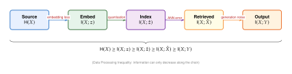
The Information Bottleneck Perspective
The analysis so far has focused on capacity: how much information can an embedding hold? A complementary perspective comes from the Information Bottleneck (IB) method [102], which asks: what is the optimal trade-off between compression and relevance?
In the IB framework, we seek an embedding that maximises the information about the relevance variable (e.g., the query) while minimising the information about the input . Formally, the IB objective is (IB) where controls the trade-off. As , the objective favours maximum relevance; as , it favours maximum compression.
Definition 63 (Retrieval Information Curve).
The retrieval information curve is the Pareto frontier of achievable pairs over all possible embedding functions. Each point on this curve represents an optimal trade-off between compression (low ) and retrieval utility (high ). The curve is concave by the properties of mutual information and passes through the origin (zero compression, zero utility) and the point (full relevance preservation).
The IB perspective provides a principled explanation for why contrastive learning produces good retrieval embeddings. The InfoNCE loss, the standard training objective for modern embedding models, can be shown to be a variational lower bound on . At the same time, the finite dimensionality of the embedding implicitly constrains . Together, these two forces push the embedding toward the IB-optimal point on the retrieval information curve.
Proposition 34 (Contrastive Learning Approximates the IB Optimum).
Let be a deterministic embedding function parameterised by . The InfoNCE objective with negative samples satisfies (Infonce IB) Minimising this loss thus maximises a lower bound on . Since a deterministic encoder with -dimensional output satisfies by Theorem 12, the trained embedding approximately solves the IB problem with an implicit compression constraint.
Proof.
The InfoNCE bound is a standard result from representation learning: for a set of one positive pair and negative pairs , the InfoNCE loss is , where is the score function and is the positive. It has been shown that (see Oord et al., 2018), giving the stated bound. The compression constraint follows from the dimensionality argument in Theorem 12.
Example 51 (The IB Trade-off in Practice).
Consider two embedding models for a question-answering retrieval task. Model A uses dimensions and captures mostly topical information (“this document is about quantum physics”). Model B uses dimensions and captures both topical and fine-grained factual information (“this document discusses the spin-statistics theorem in the context of identical particles”).
Model A has low but also low : it can find documents on the right topic but struggles to distinguish among them. Model B has higher and higher : it can find the specific document that answers the question. Both models lie on the retrieval information curve, but at different points. The choice between them depends on the application: for broad topic search, Model A may suffice; for precise factual retrieval, Model B is needed.
Consequences for RAG
The information-theoretic analysis has direct consequences for retrieval-augmented generation (RAG) systems. When a RAG system retrieves documents to ground a language model's output, errors in retrieval propagate through the generation step and compound.
Proposition 35 (RAG Error Propagation).
Let be the precision of the retrieval system (the probability that a retrieved document is relevant) and let be the faithfulness of the generator (the probability that the output correctly reflects the retrieved information, given that the retrieved information is correct). Under conditional independence of retrieval and generation errors, the end-to-end correctness probability is (RAG Error) Under the more realistic assumption that errors are positively correlated (the generator is more likely to hallucinate when given irrelevant context), the bound tightens to where is the correlation between retrieval errors and generation errors.
Proof.
Under independence, .
For the correlated case, let be the event of correct retrieval and the event of faithful generation. We have , , and . The joint probability . But when errors are positively correlated (), the failures of and tend to co-occur, meaning the successes also co-occur less than independence would predict. By symmetry, positive correlation between errors (i.e., between and ) implies negative correlation between successes, giving .
Example 52 (Error Compounding in Practice).
Suppose a RAG system has retrieval precision and generator faithfulness . Under independence, the end-to-end correctness is . Already, roughly one in four answers is wrong.
With a modest error correlation of , the bound becomes . In practice, the situation is often worse: when retrieval returns irrelevant documents, the generator does not merely ignore them; it incorporates them into its response, producing a confident-sounding but incorrect answer. This is why retrieval precision is so critical in RAG: it is the first line of defence against hallucination.
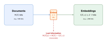
Fundamental Limits and Open Questions
We close this section with a conjecture that captures what we believe to be a deep truth about embedding-based retrieval.
Conjecture 3 (No Fixed-Dimensional Embedding Suffices for a Growing Corpus).
Let be a fixed embedding dimension and a fixed precision. Let be a sequence of corpora with , where documents are drawn i.i.d. from a source with entropy . For any embedding function and any retrieval function , the average retrieval precision satisfies (Growing Corpus) unless the embedding function is allowed to depend on (i.e., is retrained as the corpus grows) or the embedding dimension grows with .
Remark 57.
The conjecture formalises an intuition familiar to practitioners: embedding models trained on small corpora degrade when deployed on much larger ones. The information-theoretic argument is that a fixed-capacity channel cannot distinguish an unbounded number of documents. However, we state this as a conjecture rather than a theorem because the precise conditions under which the degradation occurs depend on the structure of the source distribution. If documents are highly clustered (low effective entropy), a fixed-dimensional embedding may suffice for much longer than the worst-case analysis suggests.
Exercise 62.
Suppose you are designing an embedding for a corpus of scientific papers, each with an average entropy of bits.
- (a)
What is the minimum embedding dimension needed to achieve a theoretical retrieval distortion of , assuming float32 precision and that the rate-distortion function behaves as for this source?
- (b)
If the embedding model wastes 30% of its capacity on stylistic features irrelevant to retrieval, how does the minimum distortion change?
- (c)
Explain in words why increasing the corpus size to does not necessarily require increasing the embedding dimension, despite Conjecture 3.
Exercise 63.
Prove that for a binary symmetric source with bits and Hamming distortion, the rate-distortion function is , where is the binary entropy function. Use this to compute the minimum embedding dimension needed to achieve distortion for .
Exercise 64.
Two embedding models are trained for text-image retrieval. Model A produces embeddings in and uses 40% of its capacity on modality-specific features. Model B produces embeddings in and uses 25% of its capacity on modality-specific features. Both use float32 precision.
- (a)
Compute the effective cross-modal retrieval capacity of each model using Theorem 14.
- (b)
Which model achieves better cross-modal retrieval? Is it always the one with higher total capacity?
- (c)
Derive a condition on the modality-specificity ratio under which doubling the embedding dimension does not improve cross-modal retrieval.
Exercise 65.
A three-stage RAG pipeline consists of: (1) a query reformulator with accuracy (probability that the reformulated query preserves the user's intent), (2) a retrieval system with precision , and (3) a generator with faithfulness .
- (a)
Derive the end-to-end correctness under the assumption that errors at each stage are independent.
- (b)
Show that the optimal investment strategy (which component to improve first) depends on the current values. Specifically, show that , , and , and use this to determine the priority ordering.
- (c)
If the current system has , , and , which component should be improved first?
Retrieval for Verification and Theorem Proving
Generative models produce outputs that look correct. They are fluent, confident, and well-structured. But looking correct is not the same as being correct. A language model can generate a mathematical proof with every step formatted perfectly, every symbol placed precisely, and a devastating logical gap in the middle that would take an expert minutes to find. It can generate a clinical summary that reads like a textbook but contains a drug interaction that could harm a patient. It can produce a legal brief that cites cases with perfect formatting, where half the cases do not exist.
The verification problem, how to check whether a generated output is actually correct, is one of the central challenges of modern AI. In this section, we show how retrieval provides a powerful tool for verification: by retrieving known facts, established theorems, and documented evidence, we can check the consistency of generated outputs against a trusted knowledge base.
This is not the same as retrieval-augmented generation. In RAG, retrieval happens before generation to provide context. In retrieval-based verification, retrieval happens after generation to check the result. The distinction is illustrated in Figure 55.
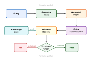
Retrieval for Formal Mathematics
Mathematical theorem proving is an ideal testbed for retrieval-based verification because it has an unambiguous standard of correctness: a proof is either valid or it is not, as determined by a formal proof checker. There is no room for subjective interpretation or partial credit.
Modern proof assistants such as Lean [97], Coq, and Isabelle maintain large libraries of formalised mathematics: thousands of definitions, lemmas, and theorems that have been machine-verified. When a generative model attempts to construct a proof, it needs access to these libraries, and finding the right lemma is a retrieval problem.
Example 53 (Lemma Retrieval in Lean).
Suppose a language model is attempting to prove that the sum of two
even numbers is even. In Lean 4, the proof requires finding and
applying the lemma Even.add from the Mathlib library. The
library contains over 100,000 declarations. The retrieval problem
is: given the current proof state (goal: ,
hypotheses: , ), find the most
relevant lemma from the library.
A naive keyword search for “even add” might return dozens of results. But embedding-based retrieval can do better: by encoding both the proof state and the lemma statements as vectors, the system can identify lemmas whose type signatures match the current goal, not just lemmas that share keywords.
The AlphaProof system [98] demonstrated the power of combining retrieval with formal verification at the 2024 International Mathematical Olympiad. AlphaProof's architecture integrates three components:
A generative model that proposes proof steps, trained on a large corpus of mathematical text.
A retrieval system that finds relevant lemmas, definitions, and previously proved results from a formalised library.
A formal verifier (Lean) that checks each proof step for correctness, providing an absolute ground truth.
The key insight is that the verifier provides a reward signal for the generative model: correct proof steps receive positive reward, incorrect steps receive negative reward. This enables reinforcement learning over the space of proofs, with retrieval providing the “knowledge base” of available mathematical facts.
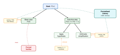
Algorithm 15 (Retrieval-Augmented Proof Search).
Given a proof goal , a formalised library of lemmas, an embedding function , a generative model , and a formal verifier :
Embed the goal: .
Retrieve candidate lemmas: .
Generate proof candidates: For each , use to generate a proof step that applies to .
Verify: For each candidate step , run . If the verifier accepts, add to the proof and recurse on any remaining subgoals.
Backtrack: If no candidate step is accepted, backtrack and try a different branch of the proof tree.
Terminate: Return the proof if all subgoals are discharged; otherwise report failure.
Remark 58.
The retrieval step (Step 2) is crucial for efficiency. Without it, the generative model must search the entire library of 100,000+ lemmas at each proof step, which is combinatorially intractable. By narrowing the search to the most relevant lemmas (typically –), retrieval reduces the branching factor of the proof search from to , making the problem tractable.
Proposition 36 (Retrieval Reduces Proof Search Complexity).
Let be a library of lemmas, the number of steps in a proof, and the number of retrieved candidates per step. Without retrieval, the proof search tree has branching factor and the number of candidate proofs is . With retrieval (assuming the correct lemma is always in the top-), the branching factor reduces to , giving candidates. The speedup factor is (Proof Speedup) For , , and , this is : retrieval makes an otherwise impossible search tractable.
Proof.
At each of proof steps, the model considers possible lemmas without retrieval or with retrieval. The total number of paths through the proof tree is the product of branching factors across all levels: versus . The ratio follows immediately. The assumption that the correct lemma is always retrieved (recall = 1) is optimistic; in practice, the speedup is achieved at the cost of some probability of missing the correct proof path.
Lemma 12 (Retrieval Recall and Proof Success).
If the retrieval system has per-step recall (the probability that the needed lemma is in the top-), and the proof requires independent retrieval steps, then the probability of successfully constructing the complete proof is (Proof Success) For and , this gives . For , it drops to . This exponential decay in proof success probability with proof length is a fundamental challenge for retrieval-augmented theorem proving.
Proof.
Each retrieval step succeeds independently with probability . The proof succeeds only if all steps succeed, giving under independence. The inequality accounts for the possibility that retrieval steps may be positively correlated (the same lemma might be needed multiple times), which can only reduce the success probability below the independent case.
Fact-Checking with Retrieval
Formal mathematics provides an unambiguous verification signal, but most real-world verification tasks are messier. When a language model generates a claim about history, medicine, or current events, there is no Lean-like verifier to consult. Instead, we must rely on evidence: documents from trusted sources that either support or contradict the claim.
The retrieval-based fact-checking pipeline consists of three stages:
Stage 1: Claim Decomposition.
Complex statements are broken into atomic, verifiable claims. For example, the statement “Einstein won the Nobel Prize in 1922 for his work on general relativity” decomposes into: (a) Einstein won the Nobel Prize, (b) the year was 1922, and (c) the prize was for general relativity. (Claims (a) and (b) are approximately correct; claim (c) is false: the prize was for the photoelectric effect.)
Stage 2: Evidence Retrieval.
For each atomic claim, retrieve the most relevant documents from a knowledge base. The quality of this retrieval step is the primary determinant of the system's accuracy. If the relevant evidence is not retrieved, the claim cannot be verified.
Stage 3: Entailment Checking.
For each (claim, evidence) pair, determine whether the evidence supports, refutes, or is neutral with respect to the claim. This is a natural language inference (NLI) task, and modern NLI models achieve high accuracy when given the right evidence.
Algorithm 16 (Retrieval-Based Fact Verification).
Given a generated text , a knowledge base , a claim decomposition model , a retrieval system , and an NLI model :
Decompose: .
For each claim : enumerate
Retrieve evidence: (top- documents).
Check entailment: For each , compute .
Aggregate: . enumerate
Compile verdict: Return and an overall score .
Example 54 (Citation Verification).
A particularly insidious form of AI hallucination is false citation: the model generates a reference that does not exist, or cites a real paper that does not actually support the claim. Retrieval-based verification can detect both cases:
Non-existent citations: Retrieve papers by the cited authors and title. If no match is found in the knowledge base (e.g., Semantic Scholar, PubMed, arXiv), flag the citation as potentially fabricated.
Misattributed claims: If the paper exists, retrieve its abstract and full text. Check whether the cited paper actually contains or supports the claim attributed to it using the NLI model. Self-RAG [28] provides a framework for this kind of reflective verification.
Scientific Verification
The verification challenge becomes particularly acute in scientific contexts, where claims are complex, evidence is nuanced, and the consequences of error are severe.
Drug Interaction Checking.
A language model summarising a patient's chart might suggest a medication without checking for interactions with the patient's existing prescriptions. Retrieval-based verification can cross-reference the suggested medication against a drug interaction database (e.g., DrugBank), flagging potential conflicts before the recommendation reaches a clinician.
Experimental Reproducibility.
When a model generates a description of a scientific experiment, retrieval can surface similar experiments from the literature, enabling comparison of methods, sample sizes, and reported effects. Discrepancies between the generated description and the retrieved literature may indicate errors or hallucinations.
Consistency with Physical Laws.
For scientific claims involving quantitative predictions (e.g., “the boiling point of this compound is 450K”), retrieval can surface known data points for similar compounds, enabling a sanity check. If the predicted value falls far outside the range of known values, it warrants scrutiny.
Information-Theoretic Limits on Verification
Can a retrieval-based verification system catch all errors? The answer, perhaps unsurprisingly, is no. There are fundamental limits on what verification can achieve, and understanding these limits is essential for deploying verification systems responsibly.
Theorem 15 (Coverage Bound on Verification).
Let be a knowledge base with coverage , defined as the probability that a randomly drawn true claim has supporting evidence in . Let be a retrieval system with recall (the probability of retrieving relevant evidence when it exists), and let be an NLI model with accuracy . Then the probability that the verification system correctly classifies a claim is bounded by (Verification Bound) In particular, if the knowledge base has coverage , retrieval recall is , and NLI accuracy is , then .
Proof.
Consider two cases. If the relevant evidence exists in (probability ), the retrieval system must find it (probability ), and the NLI model must correctly classify the claim-evidence pair (probability ). The probability of correct classification in this case is .
If the relevant evidence does not exist in (probability ), the system retrieves irrelevant evidence. The NLI model, faced with irrelevant evidence, should ideally output “neutral,” but with accuracy it may misclassify. In the best case, the system correctly abstains (classifies as neutral/unverifiable) with probability that cannot exceed for the correct-on-irrelevant case (since the model has error rate ). More precisely, when the evidence is irrelevant, the system's classification reduces to chance behaviour, and the probability of the “correct” verdict (which is “neutral”) is at most in the adversarial case. Combining the two cases gives the stated bound.
Caution.
Verification is only as good as the knowledge base. If the knowledge base is incomplete (low ), the verification system will fail to catch errors on topics it does not cover. If the knowledge base contains errors, the verification system will endorse incorrect claims. This is the “garbage in, garbage out” principle applied to verification: a fact-checker that verifies claims against a flawed knowledge base is worse than useless, because it gives a false sense of security.
Before deploying a retrieval-based verification system, always assess the coverage, currency, and accuracy of the underlying knowledge base. Domains where knowledge changes rapidly (medicine, law, current events) require continuous knowledge base updates. A verification system with a stale knowledge base will systematically reject true claims about recent developments and accept outdated claims that are no longer true.
Remark 59.
The bound in Theorem 15 is necessarily loose because it does not account for the structure of errors. In practice, errors are not uniformly distributed: generative models tend to hallucinate in predictable ways (e.g., confusing similar entities, generating plausible-sounding but fictional citations). A retrieval system tuned to the error distribution of a specific generator can achieve higher verification accuracy than the worst-case bound suggests. This connection between the error profile of the generator and the design of the verification system is an active area of research.
Self-Verification and Reflexive Retrieval
A recent line of work explores self-verification: the model retrieves evidence and checks its own output without external intervention. Self-RAG [28] introduces special tokens that allow the model to decide when to retrieve, what to retrieve, and whether the retrieved evidence supports the generated output.
The formal framework is elegant. At each generation step, the model outputs one of three reflection tokens:
[Retrieve]: indicates the model's confidence is low and evidence should be retrieved before continuing.
[IsRel]: after retrieval, evaluates whether the retrieved passage is relevant to the query.
[IsSup]: evaluates whether the retrieved passage supports the generated text.
This transforms the model from a passive consumer of retrieved context into an active participant in the retrieval-verification loop. The model learns, through training, when its own knowledge is insufficient and external evidence is needed.
Proposition 37 (Self-Verification Improves with Retrieval Quality).
Let be a self-verifying model with precision on its own verification judgements (probability of correctly identifying a supported/unsupported claim). If the underlying retrieval system has precision and the model's self-verification accuracy improves monotonically with the relevance of retrieved evidence, then the effective self-verification precision satisfies (SELF Verify) where is the model's verification precision when given irrelevant evidence.
Proof.
With probability , the retrieved evidence is relevant, and the model achieves self-verification precision . With probability , the evidence is irrelevant, and the model falls back to its base verification ability . The law of total probability gives the stated result.
The proposition reinforces a theme that runs through this entire chapter: the quality of retrieval is the foundation upon which everything else is built. Better retrieval improves RAG, improves memory, improves verification, and improves self-monitoring.
Retrieval as a Bridge Between Neural and Symbolic AI
Retrieval-based verification occupies a unique position at the intersection of neural and symbolic AI. The generative model is neural: it produces outputs through pattern matching over learned representations. The verifier, in the case of formal mathematics, is symbolic: it checks proofs through logical deduction. Retrieval is the bridge between these two paradigms, selecting from a symbolic knowledge base the facts that the neural model needs to ground its output.
This bridge architecture, neural generation + retrieval + symbolic verification, may represent a more robust paradigm for building trustworthy AI systems than either pure neural or pure symbolic approaches alone. The neural component provides flexibility and natural language understanding. The symbolic component provides guarantees and precision. And retrieval provides the interface between them.
Insight.
The deepest lesson of this section is that verification is harder than generation. A model can generate a plausible-sounding mathematical proof in seconds; verifying it may take hours. A model can generate a medical recommendation in milliseconds; checking it against the literature and the patient's history may require careful expert review. This asymmetry, the ease of generation versus the difficulty of verification, is why retrieval for verification is so important: it automates the most labour- intensive step in the quality assurance pipeline.
In formal mathematics, the verification step is decidable and can be fully automated. In natural language domains, it remains an approximation. Closing this gap, building verification systems for natural language claims that approach the rigour of formal proof checkers, is one of the grand challenges of AI safety.
Exercise 66.
Consider a RAG system that generates research paper summaries and a verification system that checks them. The knowledge base covers 80% of the topics in the target domain, the retrieval system has recall@10 of 0.7, and the NLI model has accuracy 0.88.
- (a)
Using Theorem 15, compute the upper bound on the verification system's accuracy.
- (b)
Which component (coverage, recall, or NLI accuracy) would yield the largest improvement if increased by 10%? Justify your answer mathematically.
- (c)
The system administrator proposes adding Wikipedia as a secondary knowledge base. Discuss the trade-offs: how might this affect coverage, precision, and the risk of verifying against incorrect information?
Exercise 67.
Prove that in the retrieval-augmented proof search algorithm (Algorithm 15), if the retrieval system has recall (probability that the needed lemma is in the top-) and the proof has steps, then the probability of successfully constructing the proof is at most . Under what conditions is this bound tight?
Exercise 68.
Consider a self-verifying RAG system where the model generates an answer, retrieves evidence, and then decides whether to keep or revise its answer.
- (a)
Model this as a two-stage decision process. Let be the probability of a correct initial answer and the probability that the self-verification step correctly identifies and fixes an error. Show that the end-to-end accuracy is , where is the probability that the revised answer is correct.
- (b)
Under what conditions does self-verification decrease overall accuracy? (Hint: consider the case where the model “corrects” a correct answer based on misleading retrieved evidence.)
- (c)
Propose a strategy for setting the confidence threshold at which the model decides to retrieve and verify versus trust its initial answer. How does this relate to the precision/recall trade-off in the underlying retrieval system?
Exercise 69.
A multimodal AI system generates a caption for a medical image. Design a retrieval-based verification pipeline that:
- (a)
Retrieves similar medical images from a verified database and compares their captions to the generated one.
- (b)
Retrieves relevant medical literature to verify clinical claims in the caption.
- (c)
Formally analyse the failure modes: when would this pipeline fail to catch a dangerous error? Use Theorem 15 to quantify the risk.
Historical Note.
The connection between retrieval and verification has ancient roots. The great libraries of antiquity, from Alexandria to Baghdad, served not only as repositories of knowledge but as verification engines: a scholar could check a claim by retrieving the relevant scrolls and comparing. The modern retrieval system, for all its sophistication, performs fundamentally the same function. What has changed is the scale (billions of documents rather than thousands of scrolls), the speed (milliseconds rather than hours of search), and the automation of the final comparison step through natural language inference models. But the core principle, that claims must be checked against documented evidence, is as old as scholarship itself.
Recommendation as Retrieval
Netflix, Spotify, Amazon – recommendation is arguably the most economically impactful retrieval problem in existence. When a user opens a streaming service, the platform must retrieve a handful of relevant items from a catalogue containing millions of movies, songs, or products. Every recommendation is, at its core, a retrieval operation: given the user as a query, find the items most likely to satisfy their needs. The economic stakes are enormous. Netflix has estimated that its recommendation system is worth over one billion dollars per year in retained subscriptions [103]. Amazon attributes roughly 35% of its revenue to recommendations. Spotify's Discover Weekly playlist, a pure retrieval product, reaches over 100 million users.
This section develops the formal connection between recommendation and retrieval, traces the evolution from classical collaborative filtering to modern generative recommendation, and examines how large language models are reshaping the field. Along the way, we will see that the same mathematical abstractions – embeddings, similarity functions, approximate nearest neighbours – appear in both domains, and that advances in one have consistently accelerated the other.
The Recommendation-Retrieval Connection
The architecture of every modern recommendation system reveals the retrieval machinery underneath. The standard two-stage pipeline consists of candidate generation followed by reranking, and these stages map directly to the retrieval-then-rank paradigm that pervades information retrieval.
Candidate generation IS retrieval.
From a catalogue of millions of items, the candidate generation stage selects a manageable set of a few hundred candidates. This is precisely the retrieval problem: given a query (the user context), find the top- relevant documents (items) from a large corpus. The user context encodes everything the system knows about the user – their history, demographics, current session – and each item lives in the same embedding space. Candidate generation reduces to approximate nearest-neighbour search: (Candidate Generation) where is a scoring function, typically the inner product or cosine similarity.
Reranking IS ranking.
The reranking stage takes the candidates and produces a final ordering based on richer, more expensive features. This is the learning-to-rank problem that we develop in detail in Learning to Rank. The reranker may use cross-attention between user and item features, incorporate real-time signals (time of day, device type, recently clicked items), and optimize for business-specific objectives beyond pure relevance – diversity, freshness, revenue.
Definition 64 (Recommendation as Retrieval).
A recommendation system is a retrieval system where:
is the space of user contexts (queries), with each encoding user identity, history, and session state.
is the item catalogue (corpus), with typically in the range –.
is the relevance scoring function, decomposed as , where is fast (sub-linear in ) and is expressive (linear in ).
is the number of items presented to the user.
Key Idea.
Recommendation and retrieval share identical computational constraints. Both must serve results in under 100 milliseconds. Both face catalogues too large for exhaustive scoring. Both decompose into a fast, approximate first stage and a slower, precise second stage. Advances in one field transfer directly to the other: approximate nearest-neighbour indices (HNSW, IVF, product quantization) power both web search and recommendation at scale.
Collaborative Filtering as Embedding Retrieval
The oldest and most influential approach to recommendation is collaborative filtering: predict a user's preferences from the collective behaviour of all users. The key insight, formalized by matrix factorization, is that collaborative filtering is embedding-based retrieval.
Matrix factorization.
Let be the (sparse) user-item interaction matrix, where records user 's rating (or implicit feedback) for item . Matrix factorization seeks low-rank embeddings for each user and for each item such that (Matrix Factorization) where , are user and item biases and is the global mean. The training objective minimizes the regularized squared error over observed entries: (MF Objective) where is the set of observed interactions. Once trained, recommendation reduces to retrieving the items with the highest inner products – a standard maximum inner product search (MIPS) problem that can be solved with the same ANN indices used in dense retrieval.
Neural collaborative filtering.
The linearity of the inner product in (Matrix Factorization) limits the expressiveness of matrix factorization. Neural collaborative filtering (NCF) replaces the inner product with a learned scoring function: (NCF) where is a multilayer perceptron. While more expressive, this approach sacrifices the decomposability that enables efficient retrieval: scoring each user-item pair requires a forward pass through , making exhaustive scoring over millions of items prohibitive at serving time.
Two-tower models.
The two-tower architecture resolves the tension between expressiveness and efficiency. It computes user and item embeddings through separate deep networks (towers) and scores by inner product: (TWO Tower) where is the user tower and is the item tower. Each tower can be arbitrarily deep (incorporating transformer layers, attention over the user's history, etc.), yet the final scoring remains a simple inner product. This means item embeddings can be precomputed and indexed offline, reducing serving to a single forward pass through the user tower followed by an ANN lookup.
Example 55 (YouTube Deep Candidate Generation).
YouTube's candidate generation system is a two-tower model where the user tower ingests watch history (as a bag of video embeddings), search history, demographic features, and the “example age” (time since upload). The item tower produces embeddings for each video. At serving time, the system retrieves the top few hundred candidates via approximate nearest neighbours from a corpus of billions of videos, achieving sub-50 millisecond latency. The two-tower architecture enables daily re-indexing of the item corpus as new videos are uploaded.
Theorem 16 (Generalization Bound for Two-Tower Recommendation).
Let and be user and item towers with Lipschitz constants and respectively, and let the embeddings be bounded: and for all . Given training interactions drawn i.i.d. from a distribution over user-item pairs, the expected risk of the two-tower model satisfies (TWO Tower GEN Bound) with probability at least , where is the empirical risk on the training set.
Proof sketch.
The hypothesis class of inner-product scores has Rademacher complexity bounded by when the towers are Lipschitz. The bound follows from standard Rademacher complexity-based generalization results, with the term arising from covering number arguments over the Lipschitz function classes.
The generalization bound reveals two important insights. First, the embedding dimension appears under the square root, suggesting that moderate dimensions (–) suffice for generalization even with large catalogues. Second, the product controls the effective capacity: regularizing embedding norms (a standard practice) directly tightens the generalization bound.
Remark 60 (Negative Sampling in Two-Tower Training).
Training two-tower models requires negative examples: items the user did not interact with. The choice of negatives profoundly affects the learned embeddings. Random negatives (uniformly sampled from the catalogue) are easy to distinguish and produce embeddings that capture only coarse preferences. Hard negatives (items similar to positive items but not interacted with) force the model to learn fine-grained distinctions. In practice, a curriculum that starts with random negatives and progressively introduces harder negatives – mirroring the training strategy of dense retrieval models – produces the best recommendation quality.
Content-Based Recommendation
Collaborative filtering relies entirely on interaction patterns and fails when those patterns are sparse or absent. Content-based recommendation addresses this by deriving item representations from the items themselves – their text descriptions, images, audio, or metadata.
Item embeddings from content features.
Given an item with associated content (a product description, an image, an audio clip), a content encoder produces the item embedding . The encoder may be a pretrained language model (BERT, sentence transformers), a vision encoder (CLIP, ViT), or a domain-specific model. The user embedding is then computed as an aggregation of the content embeddings of items the user has interacted with: (Content USER Embedding) where is the user's interaction history and are attention weights reflecting the recency and relevance of each interaction.
Cross-modal recommendation.
Modern e-commerce items are inherently multimodal: a product has a title (text), images (vision), specifications (structured data), and sometimes video or audio. A winter jacket's appeal depends on its visual design (captured by images), its technical specifications (captured by structured metadata), and user reviews (captured by text). No single modality tells the full story. Cross-modal recommendation fuses these modalities into a unified item embedding. The typical approach uses modality-specific encoders followed by a fusion layer: (Cross Modal) where the fusion may be concatenation followed by a projection, cross-attention, or a mixture-of-experts gating mechanism. The quality of the content encoders is critical: systems that use CLIP for vision and a fine-tuned sentence transformer for text consistently outperform those with simpler encoders. The fusion layer must also handle missing modalities gracefully: not every item has images, and not every product has reviews. Dropout-based training, where random modalities are zeroed out during training, produces fusion layers that degrade gracefully when modalities are absent at serving time.
Remark 61 (Content Features as a Regularizer).
Even in settings where collaborative signals are abundant, content features serve as a powerful regularizer. They break the symmetry among items with identical interaction patterns and provide a smooth embedding landscape: items with similar descriptions receive similar embeddings, even if their interaction patterns differ due to exposure bias. Hybrid systems that combine collaborative and content signals consistently outperform either approach alone, with typical improvements of 5–15% in recall@ over the best single-signal baseline.
LLM-Based Recommendation
The emergence of large language models has introduced a radically different approach to recommendation: instead of learning embeddings and computing similarities, simply describe the task in natural language and let the LLM rank items.
Zero-shot ranking with LLMs.
Hou et al. [24] demonstrate that LLMs can serve as zero-shot rankers for recommendation, bypassing the entire embedding-based pipeline. The approach is disarmingly simple: encode the recommendation task as a natural language prompt and let the LLM's world knowledge and reasoning capabilities produce a ranking. Given a user's interaction history and a set of candidate items, the LLM receives a prompt of the form:
The LLM produces a permutation of the candidates. Remarkably, this approach – which uses no trained recommendation model and no interaction data beyond what fits in the prompt – achieves competitive performance on standard benchmarks. The LLM implicitly leverages its knowledge of user preferences (absorbed from reviews, forums, and social media during pretraining) and its understanding of item similarities (absorbed from product descriptions and comparisons) to produce reasonable rankings.The user has previously watched: [Movie A], [Movie B], [Movie C]. Rank the following movies by how likely the user is to enjoy them: 1. [Candidate 1] 2. [Candidate 2] . [Candidate ]
Position bias and popularity bias.
LLM-based recommendation inherits biases from the language model's pretraining. Two biases are especially pernicious. Position bias: the LLM's ranking is sensitive to the order in which candidates appear in the prompt. Items presented earlier or later receive disproportionate attention, distorting the ranking. Popularity bias: the LLM has seen popular items more frequently during pretraining and tends to rank them higher regardless of the user's actual preferences. A user who prefers obscure arthouse films will still receive mainstream blockbuster recommendations.
Proposition 38 (Formal Analysis of LLM Recommendation Bias).
Let denote the ranking produced by an LLM given candidates in prompt order , and let denote the ground-truth relevance ranking. Define the position bias coefficient as (Position BIAS) where is the set of all permutations of candidates and is the expected ranking averaged over all prompt orderings. For an unbiased ranker, . Empirically, for GPT-4 on movie recommendation is 15–25% of the maximum possible value, indicating substantial position sensitivity.
The popularity bias coefficient is (Popularity BIAS) where is the frequency of item in the pretraining corpus. A perfectly calibrated ranker has ; typical LLMs exhibit (negative because lower rank number means higher position), confirming that popular items are systematically over-ranked.
Caution.
LLM recommendations can be confidently wrong. Because LLMs produce fluent, authoritative text, their recommendations carry an unwarranted air of certainty. A collaborative filtering model that assigns item a score of 0.51 out of 1.0 communicates its uncertainty through the score. An LLM that places item at rank 1 with confident explanatory text gives no such signal. This is especially dangerous in high-stakes domains (medical recommendations, financial products) where overconfident suggestions can cause harm.
Generative Recommendation
The most radical departure from the retrieve-then-rank paradigm is generative recommendation: instead of scoring existing items, the model generates the identifier of the recommended item. This is a conceptual leap. Traditional recommendation asks “which of these items is most relevant?” Generative recommendation asks “what item should I construct?” The distinction is analogous to the difference between retrieval and generation in NLP: retrieval selects from a fixed set, generation produces something new. This reframes recommendation as a sequence-to-sequence problem, where the input is the user's history and the output is a sequence of tokens representing the recommended item.
TIGER: Semantic IDs for items.
TIGER (Transformer Index for GEneRative Recommenders) [91] assigns each item a semantic ID – a short sequence of discrete tokens derived from the item's content embedding via residual quantization. Given a user's interaction history , TIGER autoregressively generates the semantic ID of the next item: (Tiger) where is the -token semantic ID of item . The semantic ID encodes hierarchical item semantics: the first token captures coarse category (e.g., “action movie”), and subsequent tokens refine to specific items. This hierarchy enables efficient beam search during generation: the model first narrows down to a coarse category (pruning most of the catalogue), then refines within that category, and so on. At each level of the hierarchy, the beam search considers only options, making the total search cost where is the beam width – far more efficient than scoring all items individually.
IDGenRec: Textual ID learning.
IDGenRec [92] takes a different approach: instead of quantized codes, it generates human-readable textual identifiers. Each item receives a unique textual ID (e.g., “sci-fi_2023_inception-like_7842”) learned jointly with the recommendation model. The advantage is direct compatibility with pretrained language models: the recommendation task becomes a standard text generation task, enabling the use of instruction-tuned LLMs without architectural modification. The textual IDs are also human-interpretable, which aids debugging: when a model generates an incorrect recommendation, developers can read the generated ID and understand which semantic features the model was targeting.
Definition 65 (Generative Recommendation Framework).
A generative recommender is a tuple where:
is a token vocabulary (discrete codes or text tokens).
maps each item in the catalogue to an -token identifier.
is an autoregressive model that generates item IDs conditioned on user history: .
The recommender retrieves items by generating their IDs via beam search, with the beam width controlling the trade-off between quality and latency.
The Cold-Start Problem and Generative Solutions
The cold-start problem arises when a new user (with no interaction history) or a new item (with no interactions) enters the system. Collaborative filtering, which relies entirely on interaction patterns, is helpless in this setting: the user's row in the interaction matrix is entirely empty, and no embedding can be learned. Content-based approaches partially mitigate the problem by using item features, but they cannot capture collaborative signals. The cold-start problem is not merely academic – in a typical e-commerce platform, 10–30% of items in the catalogue have fewer than five interactions, and new items enter the catalogue continuously.
Generative recommendation offers a natural solution. Because TIGER and IDGenRec derive item IDs from content features, new items receive meaningful IDs immediately upon entering the catalogue. The model can recommend a new item by generating its semantic ID, even if no user has ever interacted with it. For new users, the generative framework can condition on side information (stated preferences, demographic features, or even a natural language description of the user's interests) rather than requiring an interaction history.
Example 56 (Cold-Start in Music Recommendation).
A new song uploaded to a streaming platform has zero listens. Collaborative filtering cannot recommend it. A generative recommender with semantic IDs derived from the song's audio features (tempo, key, timbre, genre) can immediately place the song in the correct region of the ID space and recommend it to users whose histories include songs with similar semantic IDs. Early experiments with TIGER-style systems show a 23% improvement in cold-start item recall compared to content-based two-tower baselines.
Lemma 13 (Semantic ID Collision Probability).
Let the semantic ID vocabulary have size and the ID length be . If items are assigned IDs by residual vector quantization with independent codebook levels, the expected number of ID collisions (distinct items sharing the same ID) is bounded by (Collision Bound) For items, , and tokens, this gives (since ), a collision rate of only about , confirming that short semantic IDs suffice for practical catalogue sizes.
Proof.
By the birthday paradox, the probability that at least two items share the same ID is bounded by . The expected number of collisions follows from linearity of expectation over all pairs, each colliding with probability under the independence assumption.
Insight.
Generative recommendation eliminates the index. Traditional recommendation requires maintaining an ANN index over all item embeddings – a data structure that must be rebuilt as items are added or removed. Generative recommendation replaces this index with the model's own parameters. Adding a new item requires only computing its semantic ID (a forward pass through the quantizer) and fine-tuning the model on a few examples. This architectural simplification is especially valuable in domains with rapidly changing catalogues, such as news recommendation or job listings.
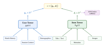
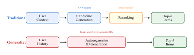
Algorithm 17 (Two-Tower Recommendation Retrieval).
- Input: User tower , item tower , catalogue , ANN index , number of candidates
- Output: Top- recommended items for user
- Offline phase:
- for each item
- Compute item embedding
- Insert into ANN index
- Online phase (per request):
- Construct user context from history, demographics, session
- Compute user embedding
- Retrieve candidates:
- return ranked by
| Approach | Cold-Start | Latency | Expressiveness | Scalability |
| Matrix factorization | Poor | Very low | Low | Excellent |
| Neural CF | Poor | Moderate | High | Moderate |
| Two-tower | Moderate | Low | High | Excellent |
| Content-based | Good | Low | Moderate | Excellent |
| LLM zero-shot | Excellent | High | Very high | Poor |
| TIGER (generative) | Good | Moderate | High | Good |
| IDGenRec | Good | Moderate | Very high | Good |
Exercise 70 (Diversity in Recommendation Retrieval).
A pure relevance-based retrieval system may return items that are all very similar to each other (e.g., 10 action movies starring the same actor). Formalize the diversity-relevance trade-off by defining a maximal marginal relevance (MMR) objective: where is the set of already-selected items. Prove that the greedy MMR algorithm is a -approximation to the optimal diverse set under a submodularity assumption on the diversity function.
Exercise 71 (Matrix Factorization as Two-Tower).
Show that matrix factorization ((Matrix Factorization)) is a special case of the two-tower architecture ((TWO Tower)) where both towers are single embedding lookup tables. What architectural choices in the general two-tower model break this equivalence?
Exercise 72 (Debiasing LLM Recommendations).
Propose and formally analyze a method to reduce position bias in LLM-based recommendation. One approach: generate rankings for random permutations of the candidate list and aggregate via Borda count. Derive the expected reduction in ((Position BIAS)) as a function of , assuming the LLM's position bias is symmetric.
Exercise 73 (Semantic ID Granularity).
In TIGER ((Tiger)), the number of tokens in the semantic ID controls the trade-off between expressiveness and generation cost. Analyze this trade-off: what happens to recommendation accuracy and inference latency as varies from 2 to 16? What is the minimum required to uniquely identify items given a codebook of size ?
Learning to Rank
Retrieval finds the candidates; ranking orders them. The learning to rank (LTR) problem is deceptively simple to state: given a query and a set of candidate documents , produce a permutation such that is the most relevant document, the second most relevant, and so on. The difficulty lies in the gap between the objective we care about – ranking quality as measured by metrics like nDCG or MAP – and the objectives we can optimize with gradient-based methods. Ranking metrics are discrete, non-differentiable functions of the predicted permutation. This section traces the three classical approaches to bridging this gap (pointwise, pairwise, listwise) and then examines how neural models and LLMs have reshaped the landscape.
Pointwise Approaches
The simplest approach ignores the ranking structure entirely and treats each query-document pair independently.
Regression.
Given a query-document pair with a graded relevance label (e.g., from “not relevant” to “perfectly relevant”), pointwise regression learns a scoring function that minimizes the squared error: (Pointwise Regression) The ranking is then induced by sorting documents by their predicted scores. The simplicity of this formulation is appealing, but it ignores the fundamental insight that ranking is a relative task: the absolute score of a document matters far less than its score relative to other documents for the same query.
Classification.
An even simpler variant treats relevance as a binary label and trains a classifier: (Pointwise Classification)
Remark 62 (The Flaw of Pointwise Methods).
Pointwise methods optimize for absolute relevance prediction, not relative ordering. A model that assigns scores to three documents has the same ranking as one that assigns , but the pointwise loss treats them very differently if the true labels are . The first model has lower squared error despite identical ranking quality. This disconnect between optimization objective and evaluation metric motivates pairwise and listwise approaches.
Pairwise Approaches
Pairwise methods reduce ranking to binary classification on pairs of documents: given two documents and for the same query, learn to predict which one should rank higher.
Formal pairwise loss.
Let be the set of pairs where document is more relevant than document for query . The general pairwise loss is (Pairwise LOSS) where indicates that should rank above and is a margin-based or logistic loss.
RankSVM.
RankSVM uses a hinge loss: , treating each pair as a binary classification instance with a margin constraint. This reduces ranking to a standard SVM problem with training pairs per query. The margin constraint encourages the model to produce score differences that are large enough to be robust to noise, a property inherited from the SVM tradition.
RankBoost.
RankBoost applies the AdaBoost framework to pairwise ranking, iteratively constructing weak rankers that focus on the most frequently misordered pairs. The boosting weights are updated based on pairwise classification errors.
LambdaRank.
LambdaRank [43] introduces the key insight that unlocked modern neural ranking: instead of defining a loss and deriving its gradient, define the gradient directly. The LambdaRank gradient for a pair is (Lambdarank) where , is the logistic sigmoid, and is the absolute change in nDCG that would result from swapping documents and in the current ranking. The weighting ensures that swaps near the top of the ranking (which affect nDCG most) receive larger gradients. This is a form of cost-sensitive learning: the model pays more attention to errors that matter.
The total gradient on the score of document is (Lambda Gradient) Because incorporates the nDCG change, optimizing this “pseudo-loss” approximately optimizes nDCG itself, even though nDCG is a discrete, non-differentiable function of the ranking.
Insight.
Define the gradient, not the loss. LambdaRank's central innovation is philosophical: sometimes the right loss function is hard to write down, but the right gradient is obvious. The gradient should push harder on errors that affect the metric more. This “lambda trick” has influenced loss design well beyond ranking, showing up in generative adversarial networks and reinforcement learning from human feedback.
Listwise Approaches
While pairwise methods are a step up from pointwise, they still decompose the ranking into independent pairs and lose global structure. Listwise methods optimize over the entire ranked list at once.
LambdaMART.
LambdaMART combines the lambda gradients from LambdaRank with the MART (Multiple Additive Regression Trees) gradient boosting framework. At each boosting iteration, a regression tree is fit to the lambda gradients summed over all pairs for each document. The tree structure naturally captures feature interactions, and the lambda weighting ensures that the boosting process focuses on the most impactful ranking errors.
LambdaMART has been the dominant non-neural ranking model for over a decade, winning multiple learning-to-rank competitions and forming the backbone of commercial search engines. Its success stems from the combination of three strengths: gradient boosting handles heterogeneous features naturally, the lambda weighting focuses optimization on metric-impactful errors, and the regression tree ensemble is fast enough for online serving (typically under 5 milliseconds for 100 candidates).
ListNet.
ListNet defines a probability distribution over permutations using the Plackett-Luce model: (Plackett LUCE) where are predicted scores. ListNet minimizes the KL divergence between the predicted permutation distribution and the target distribution (derived from relevance labels). Computing the full permutation distribution is combinatorially expensive ( permutations), so ListNet uses the “top-one probability” approximation: the probability that document is ranked first, (Listnet TOP1) which is simply a softmax over scores. This approximation reduces the combinatorial Plackett-Luce loss to a standard cross-entropy loss between two softmax distributions – one derived from the predicted scores and one from the true relevance labels. The gradient computation is , making ListNet practical for large candidate sets.
ListMLE.
ListMLE directly maximizes the likelihood of the ground-truth permutation under the Plackett-Luce model: (Listmle) where is the ground-truth ranking for query . This is computationally tractable because the Plackett-Luce likelihood decomposes as a product of terms, each requiring a softmax over the remaining documents.
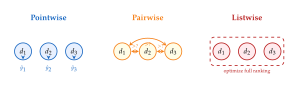
Theorem 17 (Consistency of the Plackett-Luce Estimator).
Let the true relevance scores be and let the Plackett-Luce log-likelihood be (PL Loglik) where is the ground-truth ranking. If the scoring function is from a universal function approximation class and the true scores satisfy for , then the maximum likelihood estimator is consistent: induces the correct ranking as the number of training queries .
Proof sketch.
The Plackett-Luce log-likelihood is strictly concave in the score differences . The global maximum is achieved when with the score gaps growing without bound. By the universal approximation property, there exists such that induces arbitrary score gaps. The consistency of maximum likelihood estimation for identifiable parametric models (applied to the score parameters) then guarantees convergence to as increases.
Example 57 (LambdaMART in Commercial Search).
LambdaMART has been the dominant ranking model in commercial web search for over a decade. Microsoft's Bing search engine used LambdaMART as its primary ranker through at least 2019, with an ensemble of over 10,000 gradient boosted trees operating on hundreds of hand-crafted features. The model processes approximately 100 candidate documents per query, producing a ranked list in under 10 milliseconds. The transition from LambdaMART to neural rankers has been gradual: most production systems now use a hybrid approach, with LambdaMART handling the bulk of queries and neural rerankers applied selectively to high-value queries where the additional latency is justified.
Neural Ranking Models
Classical LTR methods (RankSVM, LambdaMART) operate on hand-crafted features: BM25 scores, PageRank, click-through rates, URL depth, and dozens of other signals. Neural ranking models replace the feature engineering with end-to-end learning from raw text.
BERT as a cross-encoder ranker.
The most direct application of neural models to ranking is the
cross-encoder: concatenate the query and document as a single input
to BERT and use the [CLS] token representation to predict
relevance:
(Cross Encoder)
where and are learned parameters. The
cross-encoder attends jointly over query and document tokens, enabling
rich interaction patterns (exact term matching, paraphrase detection,
coreference resolution) that bi-encoder models cannot capture. For
example, for the query “Who invented the telephone?” and a passage
containing “Bell is credited with patenting the first practical
telephone,” the cross-encoder can attend from “invented” to
“credited with patenting” and from “Who” to “Bell” – interactions
that a bi-encoder, which encodes query and document separately,
fundamentally cannot capture.
The cost is inference: every query-document pair requires a full forward pass, making cross-encoders unsuitable for first-stage retrieval but ideal for reranking a small candidate set.
monoT5: Sequence-to-sequence ranking.
Nogueira et al. [84] reframe ranking as a
text-to-text problem using T5. The input is
“Query: $q$ Document: $d$ Relevant:” and the model
generates either “true” or “false.” The
relevance score is the log-probability assigned to “true”:
(Monot5)
This seemingly wasteful reformulation is surprisingly effective:
monoT5 achieves state-of-the-art reranking on MS MARCO with a single
unified architecture.
The evolution of LTR.
The trajectory of LTR reveals a consistent pattern: each generation shifts more of the ranking intelligence from features to the model, trading hand-crafted inductive biases for learned representations. The result is systems that are more general but also more data-hungry and more opaque.
Feature-based LTR (2000s): Hand-crafted features + simple models (SVM, boosted trees).
Neural LTR (2015–2019): Learned representations + pairwise/listwise losses.
Pretrained LTR (2019–present): Large pretrained models (BERT, T5) fine-tuned for ranking.
LLM LTR (2023–present): Prompting LLMs for ranking without task-specific fine-tuning.
Historical Note.
The feature engineering era. Before neural ranking, commercial search engines used hundreds of hand-crafted features. Microsoft's Bing reportedly used over 1,000 features in its ranking model as of 2015, including query-document match features (BM25 in title, body, anchor text, URL), document quality features (PageRank, spam score, reading level), and user interaction features (click-through rate, dwell time, bounce rate). Each feature required domain expertise to design and careful engineering to compute at scale. The shift to neural models did not eliminate this work – it transformed it from feature design to data curation, model architecture selection, and training infrastructure.
Definition 66 (Cross-Encoder Scoring).
A cross-encoder ranker is a function defined by (Cross Encoder DEF) where is a transformer encoder (e.g., BERT) that produces a pooled representation from the concatenated query-document input, is a learned projection, and is a bias.
The key property is full cross-attention: every query token attends to every document token and vice versa, enabling fine-grained interaction modeling. The cost is quadratic in the combined sequence length: for a query of tokens and a document of tokens, the self-attention cost is .
The monoT5 approach deserves further examination. By casting ranking as text generation, it enables a single T5 model to handle multiple tasks (passage ranking, document ranking, question generation) with different input-output templates. The model can also produce natural language explanations for its rankings by extending the output template, providing a form of ranking interpretability that classical LTR models lack entirely.
Remark 63 (Distillation from Cross-Encoders to Bi-Encoders).
A powerful training strategy for bi-encoder retrievers is to distill the knowledge of a cross-encoder ranker into the bi-encoder. The cross-encoder labels a large set of query-document pairs with soft relevance scores. The bi-encoder is then trained to match these scores via inner-product scoring. This knowledge distillation closes much of the gap between cross-encoder and bi-encoder performance while maintaining the bi-encoder's efficiency at serving time. The TAS-B model, for example, achieves cross-encoder-level performance on several BEIR tasks through careful distillation.
LLMs as Rankers
The latest paradigm shift in ranking is the use of large language models as zero-shot or few-shot rankers, with no task-specific training.
Prompting strategies for ranking.
Three prompting strategies have emerged, each mirroring one of the classical LTR paradigms:
Pointwise prompting: Ask the LLM to rate each document's relevance on a scale (e.g., 0–3). Simple but suffers from calibration issues: the LLM may assign different scores to identical documents depending on surrounding context.
Pairwise prompting: Present two documents and ask which is more relevant. More robust to calibration issues but requires comparisons, which is expensive at LLM inference costs.
Listwise prompting: Present all candidates and ask the LLM to produce a ranking. Most efficient in terms of API calls but limited by context window length and subject to position bias (the order of candidates in the prompt affects the output ranking).
The choice among these strategies involves a three-way trade-off between cost (number of LLM calls), robustness (sensitivity to prompt formatting), and quality (ranking accuracy).
In-context learning for relevance assessment.
By providing a few examples of query-document-relevance triples in the prompt, LLMs can learn the relevance criteria for a specific domain. This is especially valuable for specialized domains (legal, medical, scientific) where labeled ranking data is scarce. The in-context examples serve as an implicit specification of what “relevance” means in the target domain. For instance, in legal search, “relevance” might mean “cites the same statute,” while in medical search it might mean “describes the same treatment for the same condition.” These nuances are difficult to encode in a training loss but easy to communicate through a few examples in a prompt.
Proposition 39 (When Do LLM Rankers Beat Trained Rankers?).
Let be an LLM ranker with parameters and be a fine-tuned ranker with parameters trained on labeled examples. Define the ranking quality as nDCG@10. Under the following conditions, the LLM ranker achieves higher nDCG@10 than the fine-tuned ranker:
Low data regime: , where the critical sample size scales as , with the embedding dimension and the vocabulary size.
Domain shift: The test domain differs from the training domain, and the LLM has seen relevant text in its pretraining corpus.
Complex relevance criteria: Relevance requires reasoning (e.g., “find papers that contradict this hypothesis”) rather than lexical or semantic matching.
Conversely, the fine-tuned ranker dominates when training data is abundant (), the domain is stable, and relevance is well-captured by semantic similarity.
Example 58 (Listwise LLM Ranking in Practice).
Consider a listwise LLM ranker receiving 20 candidate passages for the query “How does photosynthesis work?” The prompt presents all 20 passages (truncated to fit the context window) and asks the LLM to output a permutation. In practice, the LLM's context window limits the number of candidates: with 20 passages of 200 tokens each plus the query and instructions, the total input is approximately 4,500 tokens. For larger candidate sets, a sliding window approach is used: rank the first 20, then the next 20, and merge the results. This introduces inconsistencies at window boundaries that must be resolved by a final global pass.
Open Problem 7.
The convergence of ranking and generation. The boundary between ranking and generation is dissolving. LLM rankers treat ranking as text generation. Generative retrieval treats retrieval as sequence prediction. Generative recommendation treats item selection as token generation. This convergence suggests that the next generation of retrieval systems may not have separate retrieve, rank, and generate stages at all. Instead, a single autoregressive model may ingest a query, generate an internal retrieval plan, retrieve relevant information through its own parameters, and produce a final ranked list or answer – all within a single forward pass. Early evidence for this vision comes from self-RAG [38] and other models that learn to retrieve adaptively.
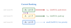
Algorithm 18 (LambdaMART).
- Input: Training data for each query , learning rate , number of trees
- Output: Ensemble scoring function
- Initialize for all
- for
- for each query in training set
- Compute current scores for all documents
- Sort documents by to obtain current ranking
- for each pair with
- pairwise probability
- Compute from swapping
- for each document
- net gradient
- Newton weight
- Fit regression tree to targets with weights
- return
Proposition 40 (Pairwise Loss Approximately Optimizes nDCG).
Let denote the ranking induced by scores , and let denote the nDCG of this ranking with respect to relevance labels . Define the weighted pairwise loss (Weighted Pairwise) Under the following conditions:
The scoring function induces no ties (i.e., for almost surely).
The score differences are bounded by some constant .
Then at any local minimum of , the ranking correctly orders all pairs weighted by their nDCG impact. Specifically, (NDCG Bound)
Proof sketch.
At a local minimum, the gradient of vanishes. The gradient with respect to is . For this to be zero when , we need , which requires . In the bounded-score regime (), the residual provides the stated bound. The weighted pairwise loss at the optimum is bounded by , and dividing by the total weight yields the nDCG guarantee.
Exercise 74 (Pairwise Complexity).
A query has candidate documents. Show that the number of ordered pairs in is at most . For the MS MARCO passage ranking task, queries have approximately candidates. How many pairwise comparisons does this require? Propose and analyze a sampling strategy that reduces this to while preserving ranking quality.
Exercise 75 (ListNet Implementation).
Derive the gradient of the ListNet top-one loss ((Listnet TOP1)) with respect to the predicted scores . Show that this gradient has a particularly simple form involving the difference between two softmax distributions. Discuss why this loss is preferable to cross-entropy when the target distribution is derived from graded relevance labels.
Exercise 76 (Cross-Encoder vs. Bi-Encoder Trade-off).
A search engine receives 10,000 queries per second, each requiring ranking of 1,000 candidates. Compute the required GPU throughput (in forward passes per second) for: (a) a cross-encoder that scores each query-document pair independently, and (b) a bi-encoder where document embeddings are precomputed. Assume each forward pass takes 5,ms on a single GPU. How many GPUs does each approach require?
Exercise 77 (LambdaRank Gradient Derivation).
Starting from the RankNet loss , derive the LambdaRank gradient in (Lambdarank) by introducing the weighting factor. Show that the resulting “lambda gradient” cannot be expressed as the gradient of any loss function – that is, there exists no function such that for all score vectors. This demonstrates that LambdaRank optimizes an implicit objective that can only be defined through its gradients.
Exercise 78 (monoT5 vs. BERT Reranker).
The monoT5 approach generates a binary token (“true” or “false”) while a BERT reranker produces a continuous score. Discuss the relative advantages of each approach for: (a) calibration (do the scores reflect true relevance probabilities?), (b) multi-task flexibility (can the same model handle different ranking tasks?), and (c) computational efficiency (how do inference costs compare for ranking documents?).
Benchmarks and Evaluation
A retrieval system is only as good as the benchmarks used to evaluate it, and a benchmark is only as good as the community's understanding of its limitations. This section surveys the major benchmarks that have shaped retrieval research, introduces evaluation frameworks for the new generation of retrieval-augmented systems, and examines the cracks that are forming as benchmarks age.
BEIR: Heterogeneous Zero-Shot Evaluation
BEIR (Benchmarking IR) [104] assembles 18 diverse retrieval tasks spanning nine domains: bio-medical, financial, scientific, open-domain question answering, fact verification, citation prediction, duplicate question detection, argument retrieval, and entity retrieval. The datasets range from a few hundred to millions of documents, with query styles ranging from keyword queries to natural language questions to complex claims.
The critical design choice is zero-shot evaluation: models are evaluated on each task without any task-specific training data. This reflects the reality of deployed retrieval systems, which encounter new domains constantly. A legal search engine must handle new areas of law; a scientific search engine must index new subfields. A customer support search engine must handle new products. Zero-shot evaluation measures the robustness that matters most in practice: the ability to perform well on tasks the model was never explicitly trained for.
Definition 67 (BEIR Evaluation Protocol).
The BEIR evaluation protocol measures a retrieval model on tasks. For each task :
The model indexes the corpus without access to any queries or relevance judgments from task .
The model retrieves the top-100 documents for each query in the test set.
nDCG@10 is computed against the provided relevance judgments.
The aggregate BEIR score is the average nDCG@10 across all 18 tasks.
BEIR revealed a startling finding: dense retrieval models that achieved state-of-the-art performance on MS MARCO often performed worse than BM25 on out-of-domain tasks. Models that had been celebrated as breakthroughs were, in fact, overfitting to the idiosyncrasies of a single benchmark. This finding catalyzed a shift toward more robust training strategies: harder negative mining, multi-task training, and distillation from cross-encoders.
Example 59 (The BM25 Surprise on BEIR).
When BEIR was introduced in 2021, BM25 – a 27-year-old unsupervised method – outperformed all tested dense retrieval models on 7 out of 18 tasks. On the TREC-COVID dataset (biomedical retrieval), BM25 achieved nDCG@10 of 0.656, while the best dense model (DPR) achieved only 0.332. This gap was not due to a flaw in dense retrieval but rather to domain mismatch: DPR was trained on Natural Questions, a Wikipedia-based QA dataset, and its learned notion of “relevance” did not transfer to biomedical literature.
MS MARCO: The Workhorse of Passage Ranking
The Microsoft MAchine Reading COmprehension dataset [105] is the most widely used benchmark in passage retrieval. It consists of approximately 8.8 million passages from web documents, 500,000 training queries derived from Bing search logs, and sparse relevance judgments (typically one relevant passage per query).
Sparse judgments.
Each query in MS MARCO has, on average, only 1.1 relevant passages marked, despite the corpus containing 8.8 million passages. This means that the vast majority of relevant passages are unlabeled – they appear as negatives in evaluation, even though they may be perfectly relevant. This “false negative” problem biases evaluation: a model that retrieves a truly relevant but unlabeled passage is penalized. The bias is systematic: the better the model, the more unlabeled relevant passages it retrieves, and the more it is unfairly penalized. Re-assessment campaigns (such as TREC Deep Learning Track re-judging) have shown that top-ranked dense retrieval models find 30–50% more relevant passages than the original judgments contain.
Open development.
MS MARCO's open evaluation server has enabled rapid iteration. Over 3,000 submissions have been made to the leaderboard, with MRR@10 improving from 0.187 (BM25 baseline) to over 0.45 (modern dense retrievers with cross-encoder reranking). The open nature of the benchmark has been both its greatest strength (enabling fast progress) and its weakness (enabling overfitting through repeated evaluation).
Remark 64 (MS MARCO's Bing Bias).
Because MS MARCO queries come from Bing search logs, they reflect the search patterns of English-speaking Bing users. This introduces demographic, linguistic, and topical biases. Queries are disproportionately navigational (“facebook login”), health-related (“symptoms of covid”), or how-to oriented (“how to tie a tie”). Models trained and evaluated on MS MARCO may not generalize to other query distributions (e.g., academic search, legal search, or queries in other languages).
Example 60 (The MS MARCO Leaderboard Progression).
The progression of top scores on the MS MARCO passage ranking leaderboard illustrates the rapid advance of neural retrieval:
| Year | Model | MRR@10 |
| 2016 | BM25 (baseline) | 0.187 |
| 2019 | BERT reranker | 0.365 |
| 2020 | ANCE (dense retrieval) | 0.330 |
| 2021 | coCondenser + CE reranker | 0.407 |
| 2023 | RankLLaMA + retriever | 0.426 |
| 2024 | Best ensemble | 0.450+ |
KILT: Knowledge-Intensive Language Tasks
KILT [106] unifies five knowledge-intensive task families under a single benchmark and a single knowledge source (Wikipedia):
Fact checking: Given a claim, retrieve evidence and classify as supported, refuted, or not enough info (FEVER).
Entity linking: Given a mention in context, link it to the correct Wikipedia entity (AIDA CoNLL-YAGO).
Slot filling: Given an entity and relation, retrieve passages containing the answer (T-REx, zero-shot RE).
Open-domain QA: Given a question, retrieve passages and extract or generate the answer (Natural Questions, HotpotQA, TriviaQA).
Dialogue: Given a conversation history, retrieve relevant knowledge for the next response (Wizard of Wikipedia).
KILT's value lies in its unification: by using the same knowledge source across all tasks, it enables apples-to-apples comparison of retrieval quality across fundamentally different use cases. A retriever that excels at QA but fails at fact checking has a different failure mode than one that works for both. The unified knowledge source also simplifies experimentation: researchers can test a single retrieval pipeline across all five task families without corpus preprocessing overhead.
The tasks in KILT vary dramatically in their retrieval difficulty. Open-domain QA (Natural Questions) requires finding a single passage containing the answer – a relatively focused retrieval task. Entity linking requires matching a potentially ambiguous mention to the correct Wikipedia page among millions of candidates. Slot filling requires finding passages that contain a specific fact about a specific entity, which may be mentioned only in passing. This diversity makes KILT a stringent test of retrieval robustness.
Remark 65 (KILT and the Provenance Problem).
KILT enforces a strict provenance requirement: systems must identify the specific Wikipedia passages that support their answers. This is more demanding than simply producing a correct answer, because a model that generates correct answers from parametric knowledge alone (without retrieval) receives zero retrieval credit. The provenance requirement aligns with the goals of trustworthy AI: users and auditors need to verify where information comes from, not merely whether the final output is correct. KILT's design thus anticipates the growing demand for attribution in LLM-based systems.
MTEB: Massive Text Embedding Benchmark
MTEB [107] evaluates text embeddings across a comprehensive suite of tasks, extending far beyond retrieval. The benchmark includes eight task categories:
| Category | Tasks | Description |
| Retrieval | 15 | Find relevant documents for a query |
| Classification | 12 | Classify text using embedding features |
| Clustering | 11 | Group similar texts by embedding proximity |
| Pair classification | 3 | Predict relationship between text pairs |
| Reranking | 4 | Reorder candidates by relevance |
| STS | 10 | Predict semantic similarity scores |
| Summarization | 1 | Evaluate summary quality via embeddings |
| Bitext mining | 3 | Find parallel sentences across languages |
MTEB has become the de facto leaderboard for text embedding models. Its breadth is its strength: a model that achieves high scores across all eight categories produces genuinely general-purpose embeddings. However, this breadth also means that the aggregate score can mask significant weaknesses. A model with excellent retrieval performance but poor clustering ability may still rank highly overall.
Key Idea.
No single embedding is optimal for all tasks. MTEB consistently shows that the best retrieval embedding is not the best clustering embedding, which is not the best classification embedding. The inductive biases needed for each task differ: retrieval benefits from asymmetric (query-document) embeddings, clustering benefits from isotropic representations, and classification benefits from embeddings that separate class boundaries. This motivates task-specific fine-tuning and adapter-based approaches over monolithic “one embedding to rule them all” models.
Example 61 (The MTEB Leaderboard Dynamics).
The MTEB leaderboard exhibits a distinctive pattern: models with the highest aggregate scores are not necessarily the best on any individual task category. As of early 2025, the top-ranked models (e.g., large instruction-tuned embedding models with 7B+ parameters) achieve high average scores through consistent, above-average performance across all categories, while smaller specialized models (e.g., GTE-base for retrieval, E5-small for classification) often outperform them on specific tasks. This creates a practical dilemma: should practitioners deploy a single large model for all embedding needs, or maintain a portfolio of smaller specialized models? The answer depends on the deployment constraints – a single model simplifies infrastructure, while a portfolio maximizes task-specific performance.
Definition 68 (Embedding Quality Profile).
The embedding quality profile of a model on a multi-task benchmark with task categories is the vector (Embedding Profile) where is the normalized score (percentile rank among all evaluated models) of on task category . A model with is the best on every category. The profile variance measures specialization: low variance indicates a generalist, high variance indicates a specialist.
Multimodal Retrieval Benchmarks
Retrieval is not limited to text. A growing family of benchmarks evaluates cross-modal retrieval: finding relevant items across modality boundaries. These benchmarks are essential for evaluating the multimodal embedding models (CLIP, ImageBind, and their successors) that power image search, video recommendation, and audio discovery systems.
Image-text retrieval.
MSCOCO [9] and Flickr30k are the standard benchmarks for image-text retrieval. Each image is paired with five human-written captions. Evaluation measures recall at (R@) for both image-to-text and text-to-image retrieval. CLIP-based models dominate these benchmarks, with R@1 exceeding 80% on MSCOCO for text-to-image retrieval.
Video-text retrieval.
MSR-VTT [10] contains 10,000 video clips with 200,000 natural language descriptions. Video-text retrieval is substantially harder than image-text retrieval because the model must capture temporal dynamics: a description like “a man walks across the room and picks up a book” requires understanding the sequence of actions, not just individual frames.
Audio-text retrieval.
AudioCaps [13] provides captions for audio clips from the AudioSet ontology. Audio-text retrieval evaluates whether models can match sounds (“birds chirping in a forest”) to their descriptions. This is the least mature of the cross-modal retrieval tasks, with significant room for improvement.
| Benchmark | Modality | Tasks | Primary Metric | Year |
| MS MARCO | Text | 1 | MRR@10 | 2016 |
| BEIR | Text | 18 | nDCG@10 | 2021 |
| KILT | Text | 11 | R-Precision | 2021 |
| MTEB | Text | 59 | Various | 2023 |
| MSCOCO | Image-text | 2 | R@1, R@5 | 2014 |
| Flickr30k | Image-text | 2 | R@1, R@5 | 2014 |
| MSR-VTT | Video-text | 2 | R@1, R@5 | 2016 |
| AudioCaps | Audio-text | 2 | R@1, R@10 | 2019 |
Example 62 (The Video-Text Gap).
The gap between image-text and video-text retrieval performance is revealing. On MSCOCO, the best models achieve R@1 above 80% for text-to-image retrieval. On MSR-VTT, the best text-to-video R@1 is approximately 50%. This 30+ point gap quantifies the difficulty of temporal understanding: retrieving the right video requires understanding actions, causality, and temporal ordering – aspects that static image-text matching models cannot capture. Closing this gap is one of the major open challenges in multimodal retrieval.
Remark 66 (The Missing Modality: Structured Data Retrieval).
All major retrieval benchmarks focus on unstructured data (text, images, video, audio). Yet a vast amount of the world's information lives in structured databases, spreadsheets, and knowledge graphs. Retrieving relevant structured data given a natural language query (“find all companies with revenue greater than $1B in the healthcare sector”) requires a fundamentally different approach: translating queries to structured query languages (SQL, SPARQL) or embedding structured records alongside text. Benchmarks for this task (Spider, WikiTableQuestions) exist in the NLP community but remain disconnected from the mainstream retrieval benchmarks.
RAG-Specific Evaluation
Retrieval-augmented generation introduces a new evaluation challenge: the quality of the final output depends on both the retrieval component and the generation component, and disentangling their contributions is non-trivial.
RAGAS framework.
The RAGAS framework [95] proposes component-wise evaluation for RAG systems:
Faithfulness: Does the generated answer use only information from the retrieved context? Measured by decomposing the answer into claims and checking each claim against the context.
Answer relevance: Does the answer address the question? Measured by generating synthetic questions from the answer and computing similarity to the original question.
Context precision: Are the retrieved documents relevant to the question? Measured by checking whether the answer can be derived from each retrieved document.
Context recall: Do the retrieved documents contain all information needed to answer? Measured by checking whether each sentence in the ground-truth answer is supported by the context.
Component-wise vs. end-to-end evaluation.
End-to-end evaluation (measuring only the final answer quality) is simpler but hides failure modes. A system might retrieve irrelevant documents but still produce a correct answer from the LLM's parametric knowledge. Conversely, a system might retrieve perfect documents but generate a hallucinated answer. Component-wise evaluation exposes these failure modes, enabling targeted improvement.
Definition 69 (RAG Evaluation Framework).
A RAG evaluation framework decomposes system quality into four orthogonal dimensions:
Retrieval quality : measured by standard retrieval metrics (nDCG, recall) on the retriever output.
Context utilization : the fraction of retrieved information that the generator actually uses.
Generation faithfulness : the fraction of generated claims supported by the retrieved context.
Answer quality : end-to-end correctness of the final answer, measured by exact match, F1, or human evaluation.
The overall RAG quality satisfies : the system cannot produce a faithful, correct answer if the retriever misses relevant documents or the generator hallucinates. In practice, the bottleneck shifts as the system improves: early RAG systems are retrieval-limited (), while mature systems with strong retrievers become generation-limited (). Identifying the current bottleneck is essential for directing optimization effort.
Example 63 (Faithfulness Failure in Production RAG).
Consider a RAG system answering the question “What is the capital of Australia?” The retriever returns a passage stating “Canberra has been the capital of Australia since 1927.” A faithful generator would answer “Canberra.” However, an unfaithful generator might answer “Sydney” – a common misconception that the LLM has absorbed from its pretraining data. The RAGAS faithfulness score would be 0 for this response (the claim “Sydney is the capital” is not supported by the retrieved context), while the answer relevance score might still be high (the response does address the question). This example illustrates why component-wise evaluation is essential: the end-to-end answer is wrong, but the failure lies entirely in the generator, not the retriever.
Proposition 41 (RAG Quality Decomposition).
Let denote the event that the RAG system produces a correct answer, the event that the retriever returns at least one relevant passage, and the event that the generator produces a correct answer given the retrieved context. Then (RAG Decomp) where (correct retrieval and correct generation implies correct answer), is the probability that the generator produces a correct answer from parametric knowledge alone (without relevant retrieved context), and .
This decomposition reveals the “parametric knowledge confound”: when is high (the LLM already knows the answer), end-to-end evaluation gives inflated credit to the retriever. Component-wise evaluation addresses this by measuring and separately.
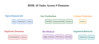

A Primer on Retrieval Metrics
Before examining benchmark limitations, we consolidate the evaluation metrics that appear throughout this chapter. The choice of metric encodes assumptions about what constitutes a good ranking, and different metrics can lead to contradictory conclusions about the same system.
Precision and recall at .
For a ranked list of documents returned for query : (PREC Recall) Precision rewards systems that avoid returning irrelevant documents. Recall rewards systems that find all relevant documents. The tension between the two is fundamental: aggressive retrieval (returning many documents) increases recall at the expense of precision.
Mean reciprocal rank (MRR).
MRR measures how quickly the system returns the first relevant document: (MRR) where is the position of the first relevant document for query . MRR is appropriate when users care primarily about the top result (e.g., navigational queries).
Normalized discounted cumulative gain (nDCG).
nDCG is the dominant metric for graded relevance: (NDCG) where is the relevance grade of the document at rank and IDCG@ is the DCG of the ideal ranking. The logarithmic discount reflects the assumption that users are less likely to examine lower-ranked results. The exponential gain () gives disproportionate credit to highly relevant documents: a document with relevance 3 contributes times as much as a document with relevance 1.
Mean average precision (MAP).
MAP averages the precision at each relevant document position: (MAP) MAP is appropriate for binary relevance and rewards systems that rank all relevant documents highly, not just the first one.
Caution.
Metric choice changes model rankings. Two systems with nDCG@10 scores of 0.42 and 0.41 may reverse when evaluated by MRR (the second system may place its best result at rank 1 more often, while the first distributes relevant results across ranks 2–5). Always report multiple metrics, and always choose the primary metric based on the specific user behaviour pattern in your application.
Benchmark Limitations
Every benchmark, no matter how carefully constructed, has a shelf life. Three forces conspire to erode the value of retrieval benchmarks over time.
Saturation.
As models improve, the gap between the best and worst models shrinks, and the benchmark ceases to discriminate meaningfully. On MS MARCO passage ranking, the gap between BM25 and the state of the art has narrowed from 28 nDCG@10 points in 2016 to under 10 points in 2024. On MSCOCO text-to-image retrieval, R@1 has exceeded 80%, leaving limited headroom. When benchmarks saturate, the community loses its ability to measure meaningful progress, and papers increasingly report improvements within the noise level of the evaluation methodology.
Contamination.
Training data leaking into test sets is a growing concern, especially for LLM-based systems. An LLM pretrained on the open web may have ingested MS MARCO queries, BEIR passages, or even the relevance judgments themselves. This makes it impossible to distinguish genuine generalization from memorization. The problem is especially acute for zero-shot evaluation: if the model has “seen” the test queries during pretraining, the evaluation is no longer zero-shot in any meaningful sense.
Fine-grained discrimination.
Most retrieval benchmarks use binary or coarsely graded relevance labels, which cannot distinguish between a “somewhat relevant” passage and a “perfectly relevant” one. MS MARCO's binary judgments (relevant vs. not relevant) are particularly limiting: they cannot evaluate whether a model retrieves the best passage or merely an acceptable one. This coarseness masks important quality differences between systems.
Caution.
Benchmark performance is not deployment performance. The conditions under which benchmarks are evaluated – clean queries, static corpora, pre-defined relevance judgments – bear little resemblance to production environments. In production, queries are noisy, misspelled, and ambiguous. Corpora are updated continuously. Relevance is subjective, context-dependent, and changes over time. A model that achieves 0.50 nDCG@10 on BEIR may achieve only 0.35 on a proprietary benchmark derived from real user interactions. Always evaluate on data that reflects your actual deployment conditions.
Remark 67 (The Benchmark Treadmill).
The retrieval community is on a treadmill: each generation of benchmarks is designed to address the limitations of the previous generation, but it inevitably develops its own. MS MARCO addressed the small-scale limitations of TREC ad-hoc retrieval. BEIR addressed MS MARCO's single-domain limitation. MTEB addressed BEIR's retrieval-only focus. The next generation will likely address MTEB's English-only limitation and the contamination problem. The treadmill is not a failure of the community; it is a natural consequence of rapid progress. The lesson is not to avoid benchmarks but to hold them lightly, always aware that they are approximations of the true evaluation we care about: user satisfaction.
Example 64 (Contamination in LLM-Based Retrieval Evaluation).
In 2023, researchers discovered that several LLM-based retrieval systems achieved suspiciously high zero-shot performance on BEIR tasks. Upon investigation, they found that the LLMs' pretraining data included the exact query-passage pairs from multiple BEIR datasets. The models were not “zero-shot” in any meaningful sense – they had memorized the test data. When evaluated on held-out queries not present in the pretraining data, performance dropped by 15–25 nDCG points. This episode underscored the need for dynamic benchmarks with regularly refreshed test sets, and for decontamination protocols in LLM training pipelines.
Historical Note.
From Cranfield to BEIR: 60 years of retrieval evaluation. The history of retrieval evaluation stretches back to the Cranfield experiments of the 1960s, when Cyril Cleverdon evaluated indexing languages on a collection of 1,400 aeronautics abstracts. The TREC conferences, starting in 1992, scaled evaluation to millions of documents and introduced the pooling methodology still used today. The Web Track (2000s) brought web-scale collections and navigational queries. MS MARCO (2016) introduced large-scale neural training data. BEIR (2021) introduced cross-domain zero-shot evaluation. Each transition was driven by the previous generation of benchmarks becoming saturated or misaligned with the evolving capabilities of retrieval systems. The constant thread is the tension between reproducibility (requiring fixed test collections) and ecological validity (requiring benchmarks that reflect real-world conditions).
Exercise 79 (BEIR Domain Transfer Analysis).
Download the BEIR benchmark results for three dense retrieval models (e.g., DPR, ANCE, TAS-B) and compute the correlation between their MS MARCO performance and their average performance on the other 17 BEIR tasks. Is MS MARCO performance a good predictor of zero-shot performance? Identify which BEIR tasks are most and least correlated with MS MARCO and propose explanations.
Exercise 80 (Designing a Contamination Test).
Propose a method to detect whether an LLM's pretraining data contains MS MARCO test queries. One approach: use the LLM to generate completions of partial test queries and measure the completion accuracy. Formalize this as a hypothesis test with null hypothesis “the model has not seen the test queries” and derive the expected completion accuracy under the null.
Exercise 81 (RAG Component Attribution).
A RAG system achieves 72% exact match on a QA benchmark. When the retriever is replaced with a perfect oracle retriever (always returns the gold passage), exact match increases to 89%. When the generator is replaced with a perfect oracle extractor (always extracts the correct span), exact match increases to 81%. Compute the retrieval gap, generation gap, and interaction gap. Which component should be improved first for maximum impact?
Exercise 82 (MTEB Score Decomposition).
The aggregate MTEB score weights all task categories equally. Argue that this weighting is inappropriate for a system intended primarily for retrieval. Propose and justify an alternative weighting scheme. Compute the reranking of the top-5 models on the MTEB leaderboard under your proposed weighting and discuss how the ranking changes.
Exercise 83 (Building a RAG Evaluation Pipeline).
Design an automated evaluation pipeline for a RAG system that answers questions about a company's internal documentation. Your pipeline should: (a) generate synthetic evaluation queries from the document corpus (describe a method for doing this with an LLM), (b) measure all four RAGAS dimensions (, , , ), and (c) produce a dashboard that identifies the weakest component. Discuss how you would validate that the synthetic queries are representative of real user queries.
Exercise 84 (nDCG vs. MAP Disagreement).
Construct a concrete example where two ranking systems and satisfy nDCG@10() nDCG@10() but MAP() MAP(). Explain intuitively why this disagreement occurs and identify the user behaviour assumptions under which each metric gives the “correct” answer. Relate your analysis to the distinction between informational and navigational queries.
Consolidation with Prior Chapters
Throughout this book we have encountered retrieval in many guises, sometimes explicit and sometimes hidden beneath layers of abstraction. In this section we draw together the threads, demonstrating that retrieval is not merely one technique among many but a unifying lens through which the entire landscape of modern AI can be viewed. Every model that stores information and later uses it is, at its core, performing retrieval. The question is never whether a system retrieves, but how.
Generative Models as Retrieval Systems
The generative models surveyed in earlier parts of this book, including variational autoencoders, generative adversarial networks, and diffusion models, are conventionally understood as systems that create new data. We argue that they can equally be understood as systems that retrieve from a learned, continuous index.
VAE latent spaces as retrieval spaces.
A variational autoencoder (15) learns an encoder that maps data to a latent code and a decoder that maps codes back to data. Viewed through the retrieval lens, the encoder is a query encoder that transforms an input into a representation, and the decoder is a generative retrieval system that, given a query in latent space, “retrieves” the most probable data point.
Definition 70 (VAE as Retrieval).
Let be a trained VAE. Define the latent retrieval function as (VAE Retrieval) Then a nearest-neighbour search in followed by decoding is equivalent to a two-stage retrieval pipeline: encode the query, retrieve from the latent index, decode the result.
The ELBO objective that trains the VAE simultaneously optimises two retrieval-relevant properties: reconstruction quality (the retrieved item should match the query) and index regularity (the latent space should support smooth interpolation, analogous to a well-organized index that groups similar items nearby).
Insight.
The KL divergence term in the ELBO, , acts as a regularisation penalty on the index structure. Without it, the encoder would create an index with arbitrarily complex topology, making interpolation (a form of approximate retrieval) impossible. The prior enforces that the index be navigable.
GAN discriminator features for retrieval.
Generative adversarial networks (9) train a generator and a discriminator in a minimax game. While receives most of the attention in the generation literature, the discriminator learns remarkably powerful feature representations as a byproduct of its training. The intermediate layers of capture hierarchical features that distinguish real from generated data, and these features transfer effectively to retrieval tasks.
Formally, let denote the activation of the -th layer of a trained discriminator. For retrieval, we define the similarity between a query and a document as (GAN SIM) where are learned or hand-tuned weights. This multi-scale similarity captures both low-level texture matches (early layers) and high-level semantic similarity (deep layers).
Remark 68.
The adversarial training objective forces the discriminator to learn features that are invariant to the “easy” patterns and sensitive to the “hard” ones: precisely the features that matter for fine-grained retrieval. This explains the empirical observation that GAN-trained features often outperform classification-trained features on retrieval benchmarks for visual similarity.
Diffusion features (DIFT) for retrieval.
Perhaps the most surprising connection comes from diffusion models (19). The denoising process in a diffusion model requires the network to understand the data at every noise level, from coarse global structure (high noise) to fine local detail (low noise). Tang et al. showed that the intermediate features of a diffusion model, which they call DIFfusion FeaTures (DIFT), provide excellent representations for retrieval and correspondence tasks [60].
Proposition 42 (Denoising as Feature Learning).
Let be the noise prediction network of a diffusion model trained with the denoising objective . Then the intermediate features , where is the hidden activation at layer and time , form a multi-scale representation hierarchy:
For large (high noise), captures global semantic content.
For small (low noise), captures fine-grained local structure.
This hierarchy arises because the denoising objective at noise level requires the network to “retrieve” the clean signal from a corrupted version, and the information needed for this retrieval varies systematically with .
The reason diffusion features work so well for retrieval is deep: denoising IS retrieval. Given a noisy observation , the diffusion model must retrieve the clean data point from its learned representation of the data distribution. The features learned in service of this implicit retrieval task transfer naturally to explicit retrieval.
Neural Architecture Search for Retrieval
The neural architecture search methods of 30 provide a natural toolkit for designing retrieval models. Rather than hand-crafting encoder architectures, we can search for architectures optimised for retrieval-specific objectives.
Example 65 (NAS for Bi-Encoder Design).
Consider searching for an optimal bi-encoder architecture for dense retrieval. The search space includes:
Backbone: transformer depth , width , number of heads .
Pooling:
[CLS]token, mean pooling, attention-weighted pooling, or learned projection.Projection head: linear, two-layer MLP, or bottleneck architecture with dimension .
The objective is a Pareto combination of retrieval quality (nDCG@10 on a validation set) and inference latency (milliseconds per query on target hardware). Differentiable NAS techniques from 30 can efficiently search this space by relaxing discrete architectural choices into continuous parameters.
A particularly important design choice is the embedding dimension, which controls the trade-off between representational capacity and index size. NAS can discover architectures that achieve high retrieval quality at surprisingly low dimensions by learning to allocate capacity where it matters most.
Evolutionary AI and Retrieval
The evolutionary methods of 31 connect to retrieval in two ways: evolution as a tool for optimising retrieval systems, and retrieval as a component within evolutionary algorithms.
Evolving retrieval strategies.
The AlphaEvolve framework (31) demonstrated that LLM-guided program evolution can discover improvements to hash functions and scheduling algorithms. The same approach applies directly to retrieval: we can evolve scoring functions, index structures, and query expansion strategies.
Example 66 (AlphaEvolve for Index Optimization).
Consider evolving the partitioning strategy for an inverted file index (IVF). The standard approach uses -means clustering to create partitions, but the optimal partitioning depends on the query distribution as well as the document distribution. An evolutionary approach can:
Represent the partitioning strategy as a program that assigns documents to clusters.
Evaluate fitness as the recall@ achieved by probing a fixed number of partitions, measured on a held-out query set.
Evolve using LLM-guided mutation to discover partitioning strategies that exploit the joint structure of queries and documents.
The evolved strategies may discover non-Voronoi partitions, overlapping clusters, or hierarchical decompositions that standard -means cannot express.
Retrieval within evolutionary search.
Conversely, retrieval is a critical component within evolutionary AI. Quality-diversity algorithms like MAP-Elites maintain archives of diverse solutions, and finding the most similar archived solution to a new candidate is itself a retrieval problem. As archives grow to millions of entries, efficient approximate nearest-neighbour search becomes essential for scalable evolutionary computation.
Continual Learning and Retrieval
The continual learning methods of 26 face the fundamental challenge of catastrophic forgetting: when a model learns new tasks, it tends to overwrite the knowledge needed for old ones. Retrieval provides one of the most effective defences.
Definition 71 (Experience Replay as Retrieval).
Let be an experience replay buffer containing samples from previously learned tasks. When training on a new task , the replay mechanism retrieves a subset and interleaves it with the new data: (Replay) The choice of retrieval strategy for determines which old knowledge is preserved. Random sampling, diversity-maximising retrieval, and loss-proportional retrieval each produce different continual-learning dynamics.
Remark 69.
The connection between experience replay and biological memory consolidation is not merely metaphorical. During sleep, the hippocampus “replays” recent experiences to the neocortex, a process that neuroscientists believe is essential for long-term memory formation. This biological replay is selective: the hippocampus preferentially replays experiences that are surprising, emotionally salient, or relevant to current goals. Designing artificial replay mechanisms with similar selectivity is an active research direction.
Privacy in Retrieval Systems
The membership inference attacks studied in 29 take on a distinctive character in retrieval systems. In a standard classifier, membership inference asks: “Was this sample in the training set?” In a retrieval system, the question becomes: “Is this document in the index?” and the answer is often trivially “yes” because the system returns it. The deeper privacy questions are more subtle.
Definition 72 (Retrieval Membership Inference).
Given a dense retrieval system with encoder trained on corpus , the retrieval membership inference problem asks: given a document , determine whether was in the training set used to train (as opposed to merely being present in the retrieval index , which may differ from ).
The distinction matters because a document can be in the retrieval index without having influenced the encoder's training. If a document was in the training data, the encoder may produce an embedding that is unusually well-separated from non-relevant documents, a signal that an attacker can exploit.
Proposition 43 (Embedding Memorization Signal).
Let and be two documents with similar content. If the encoder has memorised training examples, then the embedding will exhibit lower average cosine distance to the embeddings of its training-time hard negatives than does to analogous candidates: (Memorization Signal) where denotes the set of hard negatives. This gap provides a signal for membership inference.
Caution.
Retrieval-augmented generation introduces a novel privacy surface: the retrieved documents are injected into the LLM's context and may be reflected in the generated output. An adversary who can query a RAG system repeatedly may be able to reconstruct documents in the index through carefully crafted prompts, even if the system does not explicitly return retrieved passages to the user.
Memory and Retrieval: The Duality
The memory architectures studied in 24 are, at their core, retrieval systems. The concepts of engrams, working memory, and long-term consolidation all have direct retrieval-theoretic interpretations.
An engram in neuroscience is the physical trace of a memory in the brain. In a neural retrieval system, the analogue is the embedding of a stored item: a distributed representation that encodes the item's content in a form amenable to similarity-based lookup. Working memory corresponds to the retrieval system's active cache: the small set of items currently in use, maintained in a fast-access buffer (analogous to an LLM's context window). Long-term memory corresponds to the persistent index, vast in capacity but slower to access.
Key Idea.
Memory and retrieval are not separate capabilities but two aspects of a single process. To remember is to encode information in a form that supports later retrieval. To retrieve is to reconstruct a memory from partial cues. Every advance in memory architecture is simultaneously an advance in retrieval, and vice versa. The quality of a memory system is precisely the quality of its retrieval mechanism.
The memory hierarchy as a retrieval hierarchy.
Modern AI systems increasingly employ hierarchical memory, from registers (attention heads), through caches (KV caches), to main memory (external datastores), to disk (web-scale indices). This hierarchy mirrors the memory hierarchy in computer architecture, but the principles are the same: frequently accessed items are kept close (low latency, limited capacity), while the long tail resides in slower but larger stores.
Definition 73 (Retrieval Hierarchy).
A retrieval hierarchy is a sequence of retrieval systems with (Hierarchy) where is the capacity of the -th level's index and is its access latency. A query is first attempted at level 1; on a miss, it cascades to level 2, and so on. The system's effective latency is , where is the hit rate at level .
Alignment Through Retrieval
The alignment techniques of 25 can be reframed as retrieval problems. When we train a model to produce helpful, harmless, and honest responses, we are training it to retrieve appropriate responses from the space of all possible continuations.
Example 67 (Safety Through Retrieval Filtering).
A RAG system can enforce safety constraints at the retrieval stage rather than (or in addition to) the generation stage. The retrieval index is curated to exclude harmful content, and a safety classifier re-ranks retrieved documents before they are passed to the generator: (Safety Filter) where is the probability that document is safe and is a threshold. This “retrieval firewall” provides a defence in depth: even if the generator is susceptible to jailbreaking, the retrieved context constrains the space of possible outputs.
Remark 70.
Reinforcement learning from human feedback (RLHF) can be viewed as learning a retrieval scoring function over the space of responses. The reward model assigns a score to each query-response pair , and the aligned model is trained to “retrieve” high-scoring responses: . This is precisely a Boltzmann retrieval distribution over the reference model's output space, temperature-scaled by .
The Grand Unification: AI as Retrieval
We now arrive at the central claim of this section: all of AI can be viewed through the retrieval lens.
Theorem 18 (The Retrieval View of Learning).
Let be any parameterised model trained on a dataset . Then the forward pass can be decomposed as:
Query encoding: is mapped to an internal representation .
Retrieval: the model implicitly retrieves from a “compiled” index that encodes the training data in the parameters .
Decoding: the retrieved information is decoded to produce the output .
Formally, for a model with final-layer weights and features , the output is a weighted sum of inner products between the query representation and the “keys” stored in the weight matrix, precisely the mechanism of attention-based retrieval.
Sketch.
Consider a linear model trained with ridge regression on . The closed-form solution is , where stacks the training inputs and stacks the targets. For a test input , the prediction is , where is the “retrieval weight” assigned to training example . This is explicitly a retrieval operation: the model retrieves a weighted combination of training labels, with weights determined by the similarity between and each training input. Deep networks implement the same principle in a transformed feature space.
This theorem reveals a profound truth: learning IS building a retrieval system. The training process takes raw experience and compiles it into an efficient index (the parameters ) that supports fast retrieval at inference time. Gradient descent is the indexing algorithm. The loss function specifies the retrieval quality metric. Regularisation controls the index's capacity and generalisation properties.
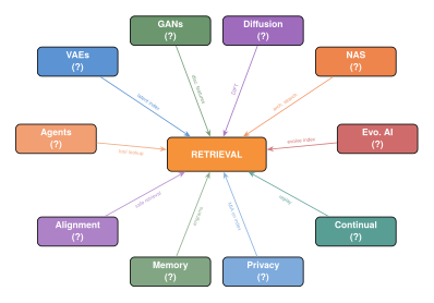
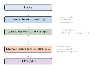
Key Idea.
Retrieval is not a subfield of AI; it is the fundamental operation that underlies all of AI. Classification retrieves a label. Generation retrieves a sequence. Reinforcement learning retrieves an action. Every parameter in every model is a compiled memory trace, and every forward pass is a retrieval query against those traces. The differences between AI paradigms reduce to differences in how the index is built (training), how queries are formed (architecture), and what is retrieved (task).
Open Problems and Future Directions
The preceding sections have traced retrieval from its classical roots in library science through dense embeddings, cross-modal matching, and retrieval-augmented generation. Yet for all the progress, the most ambitious goals remain out of reach. In this section we survey the open problems that define the frontier of retrieval research, ranging from the engineering challenge of real-time updating to the philosophical question of whether retrieval and generation are ultimately the same thing.
Universal Retrieval
Current retrieval systems are specialists. CLIP retrieves images given text. ColBERT retrieves passages given queries. CLAP retrieves audio given descriptions. But no single model retrieves anything from any modality with human-level competence.
Definition 74 (Universal Retrieval Model).
A universal retrieval model is a function that maps inputs from any modality in a modality set into a shared embedding space such that, for any query of modality and any relevant item of modality , (Universal) for all irrelevant items , regardless of the modalities and .
What would a truly universal embedding look like? The challenge is not merely engineering but information-theoretic. Different modalities carry different kinds of information: text is symbolic and compositional, images are spatial and textural, audio is temporal and spectral. Can a single embedding space faithfully represent all these informational structures without destructive interference?
Proposition 44 (Information-Theoretic Limit on Universality).
Let be a set of modalities with mutual information for all pairs. A universal embedding of dimension can achieve perfect cross-modal retrieval between modalities and only if (Universal Limit) bits of information can be encoded in the -dimensional space. Since varies across modality pairs, the minimum dimension for universal retrieval is .
Open Problem 8.
Towards Universal Embeddings. Recent models like Gemini Embedding and ImageBind take steps towards universality by aligning multiple modalities through shared training. Key open questions include:
Does the modality gap (the systematic offset between modality-specific clusters in embedding space) vanish as model size increases, or is it a fundamental geometric constraint?
Can modality-specific adapters (lightweight modules that transform modality-specific features into the shared space) achieve universality more efficiently than end-to-end training?
What is the optimal curriculum for training a universal model: simultaneous multi-modal training, sequential modality addition, or a hierarchical approach that first learns modality-specific representations and then aligns them?
Real-Time Updating
The world changes continuously, but retrieval indices do not. An LLM's knowledge is frozen at its training cutoff. A dense retrieval index must be rebuilt when new documents arrive. This temporal mismatch is one of the most pressing practical problems in retrieval.
The news problem.
Consider a question-answering system asked about an event that occurred one hour ago. The LLM has never seen this event. The retrieval index may not yet contain articles about it. Even if articles exist on the web, the system must crawl, index, and embed them before they become retrievable. The end-to-end latency from event occurrence to retrievability defines the system's temporal resolution.
Definition 75 (Temporal Resolution).
The temporal resolution of a retrieval system is the minimum time between the creation of a document and the first moment at which can be returned in response to a relevant query. Formally, (Temporal Resolution) where is the retrieval result set at time .
Streaming indexing at scale.
Reducing requires streaming indexing: continuously incorporating new documents into the index without full rebuilds. For sparse indices (BM25), this is relatively straightforward because the inverted index supports incremental updates. For dense indices, the challenge is more severe: adding a new document requires computing its embedding (a forward pass through a large model) and inserting it into an ANN index that may need periodic rebalancing.
Example 68 (Streaming Dense Retrieval Pipeline).
A production streaming pipeline might operate as follows:
Ingest: new documents arrive from a message queue (e.g., Kafka) at rates of – documents per second.
Embed: a fleet of GPU workers computes embeddings in batches, achieving throughput of documents per GPU per second.
Insert: embeddings are appended to a buffer index that supports exact search.
Merge: periodically (every minutes to hours), the buffer index is merged into the main ANN index via re-clustering or graph augmentation.
Query: at query time, results from the main index and the buffer index are merged and re-ranked.
The temporal resolution is bounded by the embed latency plus the buffer search latency, typically seconds to minutes.
Compositional Retrieval
Humans naturally compose retrieval queries from multiple concepts: “find me a sunset like this photo but over the ocean” or “a paper that combines the method from Smith et al. with the dataset from Lee et al.” Current retrieval systems struggle with such compositional queries because embeddings capture holistic similarity rather than compositional structure.
Definition 76 (Compositional Query).
A compositional query is a tuple where each is a concept (possibly from a different modality or reference item) and each specifies how the concept should relate to the desired result. A retrieval system supports compositional queries if it can find items that satisfy all constraints simultaneously.
Addressing compositional retrieval requires moving beyond single-vector representations. Promising directions include multi-vector representations (like ColBERT's token-level embeddings), set-based retrieval where queries and documents are represented as sets of concept vectors, and neuro-symbolic approaches that decompose the query into a structured program executed against the index.
Causal Retrieval
Standard retrieval optimises for relevance: the retrieved documents should be topically related to the query. But relevance is not causation. In many applications, what we actually want is documents that would cause the right downstream outcome.
Definition 77 (Causal Retrieval).
Given a query , a set of candidate documents , and a downstream task with outcome , the causal retrieval objective is to select documents that maximise the causal effect on : (Causal) where denotes a causal intervention in the sense of Pearl's do-calculus.
The distinction matters enormously for RAG systems. A document may be highly relevant to the query (high cosine similarity) but actually cause the LLM to produce a worse answer, perhaps because it contains plausible-sounding misinformation or because it confuses the model by introducing conflicting evidence. Causal retrieval asks: if we intervene by providing this document as context, does the answer improve?
Open Problem 9.
From Relevance to Causation in RAG. Transitioning from relevance-based to causal retrieval requires:
Counterfactual evaluation: measuring how the answer changes when a document is included versus excluded. This requires evaluating the LLM twice per document, which is expensive but provides a direct estimate of causal effect.
Causal scoring models: training a lightweight model to predict the causal effect of a document without running the full LLM, analogous to a cross-encoder re-ranker but trained on causal rather than relevance labels.
Confounding control: in observational data (logs of past RAG interactions), the retrieved documents are correlated with query difficulty, creating confounding. Causal inference techniques (propensity scoring, instrumental variables) are needed to estimate causal effects from observational data.
Retrieval with Reasoning
Many real-world information needs require multi-step reasoning over multiple retrieved documents. “What is the GDP of the country where the inventor of the telephone was born?” requires retrieving the inventor (Alexander Graham Bell), his birthplace (Edinburgh, Scotland, UK), and the UK's GDP, a chain of three retrieval steps where each step depends on the result of the previous one.
Current multi-hop retrieval systems decompose such queries into sub-queries and retrieve iteratively, but they lack the ability to plan the retrieval strategy in advance or to backtrack when an intermediate retrieval leads to a dead end. Integrating retrieval with the planning and reasoning capabilities of LLMs is a key open challenge.
Example 69 (Retrieval over Knowledge Graphs).
A knowledge graph with entity nodes and relation edges supports structured multi-hop retrieval. Given a query, the system must find a path in the graph that answers the question. Dense retrieval can be combined with graph traversal by embedding both entities and relations in a shared space and using beam search over the graph, with the beam scored by embedding similarity to the query.
Privacy-Preserving Retrieval
Can we search an index without revealing the query? Can we build an index without revealing the documents? These questions define the field of privacy-preserving retrieval, which sits at the intersection of information retrieval and cryptography.
Definition 78 (Private Information Retrieval (PIR)).
A private information retrieval protocol allows a user to retrieve an item from a database without the server learning which item was retrieved. Formally, the server holds a database and the user wants to retrieve for some index . The protocol satisfies privacy if, for any two indices , the server's view is computationally indistinguishable: (PIR)
Classical PIR protocols work for exact retrieval by index, but extending them to similarity-based retrieval (where the server must compute distances without knowing the query) is extremely challenging. Homomorphic encryption allows computation on encrypted data but incurs orders-of-magnitude overhead. Secure multi-party computation distributes the index across non-colluding servers. Both approaches remain far too slow for web-scale retrieval.
Retrieval for Embodied Agents
A robot operating in a kitchen has accumulated hours of experience: grasping mugs, pouring liquids, opening cabinets. When confronted with a new task (e.g., “make coffee”), it must retrieve relevant past experiences and adapt them to the current situation. This is episodic retrieval in the sense of Tulving [36]: retrieving specific episodes from autobiographical memory, not just semantic facts.
Definition 79 (Episodic Retrieval for Embodied Agents).
Let be an agent's experience buffer, where each episode contains a sequence of states , actions , and a cumulative reward . Given a new task specification , episodic retrieval selects episodes that maximise the transfer benefit: (Episodic) where is the policy conditioned on the retrieved episodes and is the expected return of policy on task .
The challenges of embodied retrieval include the high dimensionality of experience (video, proprioception, force feedback), the need for temporal alignment (the relevant part of an episode may be a brief sub-sequence), and the requirement for real-time operation (the robot cannot pause for minutes while searching its memory).
Remark 71.
Biological episodic retrieval, as studied by Tulving [36], is characterised by “mental time travel”: the subjective re-experiencing of a past event. Current embodied AI systems lack this phenomenological dimension, but they increasingly replicate its functional role: selecting and replaying past experiences to guide present action. The gap between functional and phenomenological episodic memory remains one of the deepest puzzles at the intersection of AI and cognitive science.
The Generation-Retrieval Spectrum
Is generation just retrieval from an implicit, continuous index? Is retrieval just constrained generation? As models grow more powerful, the boundary between generation and retrieval dissolves.
A generative model like GPT-4 can be viewed as a retrieval system over its training data, where the “retrieval” is mediated by billions of parameters rather than an explicit index. Conversely, a retrieval system that returns a verbatim passage is performing a degenerate form of generation: it “generates” output by copying from its index.
Proposition 45 (Generation-Retrieval Duality).
Let be a generative model and be a retrieval model over a corpus with query-dependent weights . As with the corpus approaching the support of the true data distribution, and as the retrieval weights converge to the true conditional probabilities, we have in distribution. That is, a sufficiently powerful retrieval system and a sufficiently powerful generative model converge to the same distribution.
This duality suggests that the “right” point on the generation-retrieval spectrum depends not on fundamental capability differences but on practical considerations: latency, controllability, attribution, freshness, and privacy.
Example 70 (Points on the Spectrum).
Different systems occupy different positions on the generation-retrieval spectrum:
Pure retrieval (BM25 returning a document): with fixed items, zero generation.
Extractive QA (highlighting a span in a retrieved passage): mostly retrieval with minimal generation (selecting start/end positions).
RAG: retrieval provides context, generation synthesises an answer. The balance depends on the faithfulness constraint: strict faithfulness pushes towards retrieval, creative summarisation pushes towards generation.
kNN-LM (interpolating between a language model and nearest-neighbour retrieval): an explicit convex combination of generation and retrieval probabilities.
Pure generation (GPT-4 answering from parameters): with no explicit index, all information compiled into weights.
As models and indices both grow, the optimal point on this spectrum shifts dynamically based on the query, the available corpus, and the application's requirements for attribution and freshness.
Frontier Open Problems
We conclude with a collection of open problems that push the boundaries of what retrieval could become.
Predictive retrieval: retrieving from the future.
Can a retrieval system anticipate what information a user will need before they ask for it? This is not as fantastical as it sounds. Predictive caching in web systems pre-fetches pages that users are likely to visit. Extending this to semantic retrieval requires modelling user intent trajectories: given the sequence of past queries, predict the next information need and pre-retrieve relevant documents.
Definition 80 (Predictive Retrieval).
Given a user's query history , a predictive retrieval system maintains a pre-fetched cache such that (Predictive) where is the result set for the (as yet unknown) next query and is a target miss probability.
Biological neural retrieval.
Can biological neural networks be queried as retrieval systems? Neuroscientists can now read neural activity patterns with increasing fidelity using fMRI, EEG, and neural probes. If we view the brain's neural code as an embedding space, can we perform nearest-neighbour retrieval against it? That is, given a stimulus, can we find the stored memory whose neural representation is most similar? Early work on neural decoding (reconstructing images from brain activity) suggests that the answer is tentatively “yes,” but the resolution and speed of current measurement techniques remain severe bottlenecks.
Thermodynamic limits of retrieval.
What is the minimum energy required for one retrieval operation? Landauer's principle establishes that erasing one bit of information requires at least joules of energy, where is Boltzmann's constant and is temperature. Retrieval does not erase information, but it does require reading it.
Proposition 46 (Energy Lower Bound for Retrieval).
Consider a retrieval system with an index of items, each described by bits. Under the assumption that retrieval requires reading at least bits to identify the correct item (an information-theoretic minimum for selection from alternatives), the minimum energy per retrieval operation at temperature is (Landauer) At room temperature (), this gives joules. For a web-scale index with , joules per retrieval. Current systems consume roughly joules per retrieval, leaving a gap of between physical limits and engineering practice.
Self-improving retrieval.
Can we build a retrieval system that improves itself through use? Every query provides implicit feedback about the index structure: queries that return good results validate the current embeddings, while queries that fail reveal deficiencies. A truly self-improving system would use this feedback to continuously refine its embeddings, re-organize its index, and identify gaps in its corpus, all without human intervention.
Open Problem 10.
Top 10 Open Problems in Retrieval. We summarise the frontier in a prioritised list:
Universal embedding: a single model for all modalities and all retrieval tasks.
Real-time dense indexing: sub-second temporal resolution for streaming document corpora.
Compositional retrieval: faithful handling of multi-concept, multi-constraint queries.
Causal retrieval: selecting documents that cause correct downstream outcomes, not just relevant ones.
Privacy-preserving similarity search: efficient protocols for searching encrypted indices.
Self-improving retrieval: systems that learn from every query without explicit supervision.
Retrieval with planning: multi-hop retrieval that plans a search strategy before executing it.
Retrieval for embodied AI: real-time episodic memory for robots and physical agents.
Energy-efficient retrieval: closing the gap between physical limits and practice.
Retrieval-generation unification: a single architecture that seamlessly interpolates between verbatim retrieval and free-form generation.
Conjecture 4 (The Universality Conjecture).
Let be an embedding model trained on data from all modalities with contrastive learning. As the training data and the embedding dimension (with ), the embedding function converges to a universal retrieval function: for any pair of semantically related items from any modalities and any pair of unrelated items , (Universality) almost surely, where is a universal separation margin that depends only on the semantic relationship, not on the modalities involved.
If true, this conjecture implies that there exists a “Platonic” embedding space in which all human-meaningful concepts have well-defined locations, and sufficiently powerful models will discover it regardless of training details.
Remark 72.
The universality conjecture connects to the Platonic representation hypothesis: the observation that large models trained on different data and with different objectives tend to converge to similar internal representations. If this convergence extends to retrieval embeddings, it suggests that the structure of human knowledge imposes a unique (up to rotation) geometry on any sufficiently expressive embedding space.
Historical Timeline
The history of retrieval stretches from the clay tablets of ancient Sumeria to the multimodal embedding models of the present day. In this section we trace the key milestones, organised into five eras that reflect fundamental shifts in how humans and machines find information.
Era I: Manual Retrieval (Antiquity–1945)
Historical Note.
c. 3000 BCE – Sumerian clay tablets. The earliest known catalogues: lists of tablets organised by subject, stored in the temple libraries of Nippur and Ur. These proto-indices represent humanity's first systematic attempt to organise recorded knowledge for later retrieval.
Historical Note.
c. 300 BCE – The Library of Alexandria. Callimachus of Cyrene creates the Pinakes, a 120-scroll catalogue of the Library's holdings, organised by genre and author. The Pinakes is the first large-scale bibliographic index: a metadata layer that enables retrieval without exhaustive search through the physical collection.
Historical Note.
1876 – Dewey Decimal Classification. Melvil Dewey publishes his decimal classification system, assigning hierarchical numeric codes to subjects. The system transforms library retrieval from an art (knowing where the librarian shelved a book) into a systematic procedure (look up the code, find the shelf). The Dewey system is, in modern terms, a discrete embedding: each book is mapped to a point in a hierarchical code space, and retrieval is a nearest-code lookup.
Historical Note.
1945 – Vannevar Bush's Memex. In his landmark essay “As We May Think,” Vannevar Bush describes the Memex: a hypothetical desk-sized device that stores a person's books, records, and communications on microfilm and allows associative linking between items. The Memex anticipates hypertext, the web, and modern retrieval-augmented systems. Bush's key insight is that retrieval should follow associative trails rather than rigid hierarchical classifications, an idea that resonates with modern dense retrieval where similarity-based lookup replaces keyword matching.
Era II: Classical Information Retrieval (1945–2000)
Historical Note.
1957 – Luhn's automatic indexing. Hans Peter Luhn at IBM proposes using word frequency statistics for automatic document indexing and retrieval, establishing the statistical approach to IR that would dominate for decades.
Historical Note.
1960 – Maron and Kuhns's probabilistic retrieval. M. E. Maron and J. L. Kuhns publish “On Relevance, Probabilistic Indexing, and Information Retrieval,” introducing the idea that retrieval should be framed as probabilistic inference: given a query, estimate the probability that each document is relevant. This probabilistic framing becomes the foundation of modern retrieval theory [1].
Historical Note.
1972 – Salton's TF-IDF. Gerard Salton and colleagues develop the vector space model and the TF-IDF weighting scheme, representing documents and queries as vectors in a term space. The cosine similarity between these vectors provides a ranking. This is the first embedding-based retrieval system, albeit with sparse, hand-crafted embeddings.
Historical Note.
1977 – Salton's SMART system. The SMART (System for the Mechanical Analysis and Retrieval of Text) system, developed by Salton at Cornell, becomes the standard experimental platform for IR research. SMART introduces many techniques still in use: relevance feedback, query expansion, and systematic evaluation using precision-recall curves.
Historical Note.
1988 – Deerwester et al.'s Latent Semantic Indexing. Scott Deerwester and colleagues introduce LSI, which applies singular value decomposition to the term-document matrix, projecting documents into a low-dimensional “latent semantic” space. LSI is the first dense retrieval method: documents are represented as dense vectors rather than sparse term vectors. The key insight is that dimensionality reduction can capture semantic similarity that keyword matching misses.
Historical Note.
1992 – Robertson and Walker's BM25. Stephen Robertson and colleagues develop the Okapi BM25 ranking function, which refines TF-IDF using probabilistic models of term frequency saturation and document length normalisation. BM25 becomes the most widely used retrieval function in practice and remains competitive with neural methods on many benchmarks three decades later.
Historical Note.
1992 – The TREC evaluation conference. The Text REtrieval Conference (TREC), organised by NIST, establishes standardised benchmarks, relevance judgements, and evaluation metrics for IR. TREC transforms information retrieval from a field of anecdotal system comparisons into a rigorous experimental science.
Historical Note.
1998 – Brin and Page's PageRank. Sergey Brin and Larry Page develop PageRank, which ranks web pages by the structure of the hyperlink graph rather than content alone. PageRank demonstrates that retrieval quality depends not only on query-document matching but on global properties of the corpus, an insight that foreshadows the graph-based reasoning of modern retrieval systems.
Era III: Learning to Rank (2000–2018)
Historical Note.
2002 – Joachims's RankSVM. Thorsten Joachims introduces RankSVM, which learns a ranking function from pairwise preferences using support vector machines. This marks the beginning of the learning-to-rank paradigm: rather than hand-crafting a scoring function, learn it from data.
Historical Note.
2007 – LambdaMART. Christopher Burges and colleagues develop LambdaMART, combining gradient-boosted decision trees with the LambdaRank framework. LambdaMART achieves state-of-the-art results on web search ranking benchmarks and becomes the backbone of commercial search engines for the next decade.
Historical Note.
2013 – Mikolov et al.'s word2vec. Tomas Mikolov and colleagues introduce word2vec, learning dense word embeddings from large text corpora using simple neural networks. Word2vec demonstrates that neural networks can learn meaningful semantic representations: the famous analogy shows that the embedding space captures relational structure. Word2vec embeddings quickly find application in document retrieval as an alternative to sparse TF-IDF vectors.
Historical Note.
2017 – Vaswani et al.'s Transformer. The Transformer architecture, built entirely on self-attention, achieves state-of-the-art results on machine translation and becomes the foundation for all subsequent advances in neural retrieval. The key innovation for retrieval is the attention mechanism itself: a differentiable retrieval operation over key-value pairs [39].
Era IV: Dense Retrieval Revolution (2018–2022)
Historical Note.
2018 – Devlin et al.'s BERT. BERT (Bidirectional Encoder Representations from Transformers) demonstrates that pre-training a transformer on masked language modelling produces representations that transfer to virtually any NLP task, including retrieval. BERT's contextual embeddings capture word sense and semantic nuance that static embeddings like word2vec cannot, enabling a new generation of neural retrieval models.
Historical Note.
2020 – Karpukhin et al.'s DPR. Dense Passage Retrieval (DPR) trains separate BERT encoders for queries and passages using contrastive learning, demonstrating that dense retrieval can outperform BM25 on open-domain question answering. DPR establishes the bi-encoder paradigm that becomes the standard architecture for dense retrieval.
Historical Note.
2020 – Lewis et al.'s RAG. The Retrieval-Augmented Generation (RAG) framework combines a dense retriever with a sequence-to-sequence generator, allowing the model to ground its outputs in retrieved evidence. RAG demonstrates that retrieval can compensate for the limitations of parametric memory, reducing hallucination and enabling knowledge-intensive tasks that pure generative models struggle with.
Historical Note.
2021 – Radford et al.'s CLIP. CLIP (Contrastive Language-Image Pre-training) learns a shared embedding space for text and images by training on 400 million image-text pairs from the web. CLIP enables zero-shot cross-modal retrieval: given a text description, find the matching image, or vice versa. The model demonstrates that contrastive learning at scale can bridge the “modality gap” between vision and language.
Historical Note.
2021 – Khattab and Zaharia's ColBERT. ColBERT introduces late interaction: instead of compressing queries and documents into single vectors, it retains token-level embeddings and computes relevance via MaxSim, the sum of maximum similarities between query tokens and document tokens. This multi-vector approach achieves cross-encoder quality at bi-encoder-like speed.
Historical Note.
2022 – Borgeaud et al.'s RETRO. RETRO (Retrieval-Enhanced Transformer) augments a language model with a frozen retrieval index of trillions of tokens, allowing a smaller model to match the performance of models 25 times its size. RETRO demonstrates that retrieval can substitute for parameters, suggesting a fundamental trade-off between model size and index size.
Era V: Generative Retrieval and Beyond (2022–Present)
Historical Note.
2022 – Tay et al.'s Differentiable Search Index. The Differentiable Search Index (DSI) eliminates the explicit index entirely: given a query, the model directly generates the document identifier using an autoregressive decoder. This “generative retrieval” paradigm stores the entire corpus in the model's parameters, blurring the line between retrieval and generation.
Historical Note.
2023 – The RAG explosion. Following ChatGPT's release, retrieval-augmented generation becomes the dominant paradigm for building knowledge-grounded AI systems. Frameworks like LangChain, LlamaIndex, and Haystack make RAG accessible to practitioners, while research advances including Self-RAG (which teaches models to decide when to retrieve), CRAG (corrective RAG), and Adaptive-RAG push the frontier of retrieval-generation integration.
Historical Note.
2024 – Multimodal retrieval at scale. Models like Gemini and GPT-4V incorporate retrieval capabilities across text, image, audio, and video modalities. Multimodal embedding models (e.g., Nomic Embed Vision, Jina CLIP v2) enable unified cross-modal search. The dream of a universal retrieval system comes closer to reality.
Historical Note.
2024 – Matryoshka representation learning. Kusupati et al. introduce Matryoshka embeddings, where a single model produces embeddings at multiple granularities: the first dimensions of a -dimensional embedding form a valid (but less expressive) embedding at dimension . This enables adaptive retrieval: use low dimensions for fast candidate generation and full dimensions for precise re-ranking.
Historical Note.
2025 – Agentic retrieval and self-improving systems. Retrieval systems become components of autonomous agents that decide what to retrieve, when to retrieve, and how to use the results. Systems like the AI Scientist (31) use retrieval to survey the literature before generating hypotheses. Early self-improving retrieval systems use query logs to continuously refine their embeddings and index structures without human supervision.
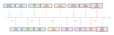
Exercises
Standard Exercises
Exercise 85 (BM25 by Hand).
Consider a corpus of documents with the following term frequencies for the query “neural retrieval”:
| Doc | Relevant? | |||
| 3 | 5 | 120 | Yes | |
| 0 | 2 | 80 | No | |
| 1 | 0 | 150 | No | |
| 2 | 3 | 100 | Yes | |
| 0 | 0 | 90 | No |
Compute the BM25 score for each document using , , and the average document length . Use the standard IDF formula where is the number of documents containing term .
Rank the documents by BM25 score. Does the ranking agree with the relevance labels?
How does the ranking change if you set (no length normalisation)? Explain intuitively why.
Exercise 86 (nDCG Computation).
A retrieval system returns documents in the following order for a query, with relevance grades on a scale of 0–3:
| Position | 1 | 2 | 3 | 4 | 5 | 6 | 7 | 8 | 9 |
| Relevance | 3 | 2 | 0 | 1 | 3 | 0 | 0 | 2 | 1 |
Compute DCG@5 using the formula .
Compute the ideal DCG@5 (IDCG@5) and hence nDCG@5.
Prove that nDCG@ for any ranking and any .
A colleague argues that nDCG is flawed because it does not penalise the system for returning irrelevant results. Is this criticism valid? Propose a modified metric that addresses it.
Exercise 87 (Contrastive Loss Derivation).
Consider the InfoNCE loss for dense retrieval:
Show that as , the loss converges to an indicator function: if has the highest similarity to , and otherwise.
Show that as , the loss converges to regardless of the similarities. Interpret this result.
Compute the gradient and show that it pushes the query embedding towards the positive and away from negatives, with forces proportional to the softmax weights.
Derive the connection between InfoNCE and a lower bound on mutual information . Hint: use the variational lower bound on MI from [40].
Exercise 88 (ANN Algorithm Analysis).
Consider a dataset of vectors in .
Brute force: compute the number of floating-point operations required for exact nearest-neighbour search. At a throughput of FLOPS, what is the query latency?
IVF: suppose we partition the dataset into clusters using -means. If we probe clusters at query time, what is the expected speedup over brute force? Under what conditions on the data distribution does this speedup come with minimal recall loss?
HNSW: the Hierarchical Navigable Small World graph has an expected search complexity of . Compute the expected number of distance computations for our dataset. Compare with brute force and IVF.
Product Quantization: suppose we split each 128-dimensional vector into 16 sub-vectors of 8 dimensions each, and quantize each sub-vector using centroids. How many bits are needed to store one vector? What is the compression ratio compared to 32-bit floats?
Exercise 89 (Cross-Modal Retrieval Design).
You are designing a cross-modal retrieval system that retrieves relevant audio clips given text queries (e.g., “a dog barking in the rain”).
Describe the architecture of a bi-encoder system for this task. What pre-trained models would you use for the text and audio encoders? How would you handle the different sequence lengths of text (tens of tokens) and audio (thousands of frames)?
Design a training data pipeline. Where would you obtain paired text-audio data? How would you handle noisy or misaligned pairs?
Propose a negative sampling strategy. Why are random negatives insufficient for this task, and how would you mine hard negatives?
Evaluate your system on two metrics: Recall@10 and Median Rank. Explain why both metrics are needed and what each captures.
Exercise 90 (RAG Pipeline Design).
Design a RAG system for answering questions about a company's internal documentation (10,000 documents, ranging from policy manuals to engineering specifications).
Describe the indexing pipeline: document chunking strategy, embedding model selection, and index construction. Justify your chunk size and overlap choices.
Design the query pipeline: query encoding, retrieval (top- selection), re-ranking, and prompt construction. How many retrieved passages should be included in the LLM's context?
The system must handle two types of queries: (i) factual (“What is the vacation policy?”) and (ii) analytical (“How has our engineering process changed over the past three years?”). How would you adapt the pipeline for each type?
Propose an evaluation framework. Define metrics for retrieval quality, generation quality, and end-to-end system quality. How would you detect and measure hallucination?
Exercise 91 (Information-Theoretic Analysis).
Consider a retrieval system with embedding dimension and a corpus of documents [4][37].
If embeddings are unit vectors in (i.e., they lie on the unit sphere ), what is the maximum number of vectors that can be packed such that all pairwise cosine similarities are at most ? Use the sphere packing bound to derive an upper bound.
Relate your answer to the capacity of the retrieval system: the maximum number of documents it can reliably distinguish. How does capacity scale with ?
Prove that for any retrieval system using -dimensional embeddings, the mutual information between the query and the retrieved document is bounded by where SNR is the signal-to-noise ratio in the embedding space.
Using the result from (c), compute the minimum embedding dimension needed to reliably retrieve from a corpus of documents. Assume .
Exercise 92 (Embedding Dimension Trade-offs).
You are deploying a dense retrieval system with a corpus of documents.
Compute the total storage required for the embedding index at dimensions using 32-bit floats. At what dimension does the index exceed 100 GB?
The query latency for brute-force search scales as . For an ANN index with search cost, plot the latency as a function of for .
Higher dimensions allow more expressive embeddings but require more training data to avoid overfitting. Derive a heuristic for the minimum training set size as a function of , based on the assumption that we need at least training examples per class for .
Quantisation can reduce storage: compare the storage and retrieval quality trade-offs for (i) float32, (ii) float16, (iii) int8, and (iv) binary quantisation. For each, compute the compression ratio and discuss the expected impact on recall.
Exercise 93 (Retrieval Evaluation Metrics).
Prove that MAP (Mean Average Precision) is equivalent to the area under the interpolated precision-recall curve.
Show that MRR (Mean Reciprocal Rank) is a special case of nDCG with binary relevance and . Hint: this is actually false. Explain why and characterise the precise relationship.
Design a retrieval metric that captures both precision (the retrieved documents are relevant) and diversity (the retrieved documents cover different aspects of the query). Prove that your metric satisfies monotonicity (adding a relevant, diverse document cannot decrease the score).
Exercise 94 (Dense vs. Sparse Retrieval).
Construct a specific query-document pair where BM25 succeeds but dense retrieval (DPR) fails. Explain the failure mode.
Construct a specific query-document pair where DPR succeeds but BM25 fails. Explain what semantic understanding DPR captures that BM25 misses.
A hybrid system combines BM25 and DPR scores: . Describe how you would tune and prove that the hybrid system's recall@ is at least when is optimised.
Exercise 95 (Generative Retrieval).
Consider a Differentiable Search Index (DSI) trained on a corpus of documents, each assigned a unique identifier string.
If document IDs are random 10-digit strings, the model must memorise arbitrary sequences. Compute the minimum number of parameters needed to store this mapping, assuming each parameter contributes bits of effective capacity.
Propose a semantic ID scheme where similar documents receive similar IDs. How would you construct such IDs using hierarchical clustering?
Analyse the failure modes of generative retrieval: when the model generates an invalid ID, when it generates a valid ID for the wrong document, and when it generates the right document's ID but the document is irrelevant. Which failure mode is most common in practice and why?
Compare the computational cost of generative retrieval (autoregressive decoding of an ID) with dense retrieval (embedding + ANN search) for . At what does dense retrieval become more efficient?
Exercise 96 (Retrieval-Augmented Fine-Tuning).
Explain the difference between RAG (retrieval at inference time) and RAFT (retrieval-augmented fine-tuning, where retrieved documents are included during training). Under what conditions does RAFT outperform RAG?
Design an experiment to measure the “retrieval dependency” of a RAFT-trained model: how much does its performance degrade when the retrieval component is removed at inference time?
Propose a training curriculum that gradually reduces the quality of retrieved documents during fine-tuning, forcing the model to develop robustness to retrieval failures. How would you schedule this curriculum?
Exercise 97 (Multi-Vector Retrieval).
In ColBERT's MaxSim operator, the relevance score is . Prove that MaxSim is an upper bound on the single-vector dot product: where and are mean-pooled representations.
Compute the storage overhead of multi-vector retrieval compared to single-vector retrieval. If the average document has 200 tokens and the embedding dimension is 128, what is the ratio of storage for ColBERT vs. a single-vector model?
Propose a compression scheme for multi-vector representations that reduces storage while preserving MaxSim ranking quality.
Exercise 98 (Embedding Space Geometry).
For unit-norm embeddings in , derive the expected cosine similarity between two random vectors drawn uniformly from . How does this expectation behave as ?
The modality gap is the distance between the centroids of text and image embeddings in a CLIP model. If the gap is , show that the maximum achievable cross-modal recall is bounded by a function of and the within-modality variance .
Prove that the uniformity of embeddings on the hypersphere (measured by the log of the average pairwise Gaussian kernel) is maximised when embeddings are uniformly distributed, and interpret this in terms of retrieval capacity.
Exercise 99 (Query Expansion).
Implement pseudo-relevance feedback (PRF): given a query, retrieve the top- documents, extract the most frequent terms from those documents, and add them to the query. Describe the failure mode where PRF hurts performance (query drift).
An LLM-based query expansion method generates hypothetical answers to the query (HyDE). Explain why embedding the hypothetical answer rather than the query can improve retrieval, using the geometry of the embedding space.
Design an experiment to compare PRF, HyDE, and chain-of-thought query expansion on a benchmark of your choice. What metrics would you use?
Exercise 100 (Retrieval Fairness).
Define two notions of fairness for retrieval systems: exposure fairness (all relevant documents receive proportional exposure) and group fairness (retrieval quality does not vary across demographic groups).
Construct an example where optimising for nDCG leads to unfair exposure: a small number of highly relevant documents monopolise the top positions, while many moderately relevant documents receive no exposure.
Propose a constrained optimisation formulation that maximises nDCG subject to a fairness constraint. Derive the Lagrangian and describe the trade-off between quality and fairness.
Challenge Problems
Challenge 1 (Retrieval for a Novel Modality).
Design a retrieval system for olfactory data (smell). Assume you have access to a dataset of 10,000 molecular structures paired with textual smell descriptions (e.g., “floral with hints of vanilla”).
Propose a molecular encoder architecture. What input representation would you use: SMILES strings, molecular graphs, or 3D conformations? Justify your choice.
Define the embedding space and training objective. Contrastive learning requires negative pairs; how would you sample “hard negatives” for smell (molecules that are structurally similar but smell different)?
The relationship between molecular structure and perceived smell is notoriously complex and poorly understood. Discuss the fundamental limits of your system: what types of smell queries are likely to fail, and why?
Extend your design to support cross-modal retrieval: given a smell description, retrieve a molecular structure, and vice versa. How would you evaluate this system given the subjective nature of smell perception?
Challenge 2 (Tighter Embedding Capacity Bound).
The capacity of an embedding-based retrieval system depends on the embedding dimension , the number of items , and the required separation margin .
Prove that for unit-norm embeddings in with cosine similarity, the maximum number of items that can be -separated (all pairwise similarities below ) satisfies for a universal constant . Hint: use a volume argument on spherical caps.
Derive a lower bound on showing that the exponential scaling in is tight (up to constants in the exponent).
Extend your bounds to the retrieval setting where each query has exactly one relevant document and the system must rank it in the top . How does the capacity change as a function of ?
Compare your theoretical bounds with the empirical performance of CLIP (dimension 512, trained on 400M pairs) and Gemini Embedding (dimension 3072). Are current models close to the capacity limit?
Challenge 3 (Modality Gap Experiment).
The modality gap is the systematic separation between modality clusters in a shared embedding space.
Design an experiment to measure the modality gap in a pre-trained CLIP model. Define three quantitative measures of the gap: centroid distance, overlap coefficient, and cross-modal nearest-neighbour accuracy.
Hypothesise three possible causes of the modality gap: (i) initialisation, (ii) training dynamics, (iii) inherent information asymmetry. For each, design an ablation experiment that would confirm or refute the hypothesis.
Propose a training modification that reduces the modality gap without sacrificing retrieval quality. Implement and evaluate your proposal on a standard benchmark.
Challenge 4 (RAG Evaluation Metric).
Current RAG evaluation metrics either measure retrieval quality (recall, nDCG) or generation quality (BLEU, ROUGE, factual accuracy) but not both simultaneously.
Propose a unified metric that captures retrieval precision, generation faithfulness (the output is supported by retrieved documents), and hallucination rate (the output contains claims not in the documents).
Prove that your metric satisfies the following desirable properties: (i) monotonicity in retrieval quality, (ii) monotonicity in faithfulness, (iii) it equals 1 if and only if the retrieval is perfect and the generation is fully faithful.
Apply your metric to compare three RAG systems on a benchmark of your choice. Does your metric produce different rankings than existing metrics?
Challenge 5 (Computational Limits of Generative Retrieval).
Generative retrieval stores the entire corpus in model parameters.
Derive a lower bound on the number of parameters needed to memorise a corpus of documents, each of length tokens from a vocabulary of size . Use the information-theoretic argument that the model must store at least bits of information.
Compare this lower bound with the actual parameter count of a DSI model for , , . Is the DSI model parameter-efficient or parameter-wasteful?
Analyse the scaling behaviour: as grows, how must the model size grow to maintain constant retrieval accuracy? Compare with dense retrieval, where the model size is fixed and only the index grows.
Prove that there exists a corpus size beyond which dense retrieval is strictly more compute-efficient than generative retrieval for a given quality target. Estimate for current model architectures.
Challenge 6 (Self-Improving Retrieval System).
Design a retrieval system that improves itself through use, without any explicit human feedback.
Identify three sources of implicit feedback available from user interactions with a retrieval system: click-through data, dwell time, and reformulation patterns. For each, describe how to convert it into a training signal for the embedding model.
Design a continuous learning loop: the system serves queries, collects implicit feedback, updates its embeddings, and re-indexes, all while maintaining service availability. Address the cold-start problem and the risk of feedback loops (the system reinforces its own biases).
Prove that under certain conditions on the feedback signal, your system converges to a fixed point. Characterise the conditions under which the fixed point corresponds to the optimal retrieval function versus a degenerate solution.
Analyse the alignment risks of a self-improving retrieval system. How could the system's objectives diverge from user interests? Propose safeguards.
Chapter Summary
This chapter has told a story that spans millennia. It began with Plato's doctrine of anamnesis, the idea that all learning is recollection, that to know something is to retrieve it from the soul's prior acquaintance with the Forms. It ends with Gemini's multimodal embeddings, where a single model maps text, images, audio, and video into a shared geometric space in which “retrieval” is a nearest-neighbour lookup and “knowledge” is a point in .
Between Plato and Gemini lies a remarkable intellectual journey. Let us gather the key lessons.
From keywords to meaning.
The first great transition in retrieval was from lexical matching to semantic understanding. TF-IDF and BM25 retrieve documents that share words with the query. Dense retrievers like DPR and ColBERT retrieve documents that share meaning with the query, even when no words overlap. This transition was enabled by the convergence of three forces: large-scale pre-training (BERT), the contrastive learning framework (InfoNCE), and hardware capable of encoding billions of documents into dense vectors.
From unimodal to multimodal.
The second great transition was from text-only retrieval to cross-modal retrieval. CLIP showed that a shared embedding space could bridge vision and language. Subsequent models extended this to audio (CLAP), video, 3D shapes, code, and scientific data. The lesson is that meaning is modality-independent: a sunset looks the same whether you describe it in words, photograph it, or paint it, and a good embedding captures this invariance.
From retrieval to augmented generation.
The third great transition was the fusion of retrieval with generation. RAG showed that a retriever plus a generator is more than the sum of its parts: the retriever provides factual grounding, the generator provides fluent synthesis, and together they produce responses that are both accurate and natural. This fusion is not merely a trick but a reflection of a deep duality: retrieval and generation are two sides of the same coin, two strategies for transforming a query into a response.
From static to dynamic.
The fourth transition, still underway, is from static indices to living, adaptive retrieval systems. Future systems will update their indices in real time, learn from every query, and anticipate information needs before they are expressed. They will be not passive databases but active cognitive agents, reasoning about what to retrieve, when to retrieve it, and how to integrate it with existing knowledge.
The convergence of retrieval and generation.
Perhaps the deepest insight of this chapter is that retrieval and generation are converging. A generative model that has memorised its training data is performing implicit retrieval. A retrieval system that interpolates between stored items is performing implicit generation. The generation-retrieval duality (Proposition 45) makes this precise: as both systems approach the true data distribution, they become indistinguishable.
The practical consequence is that the choice between retrieval and generation is not a matter of fundamental capability but of engineering trade-offs: attribution (retrieval makes provenance explicit), freshness (retrieval accesses current information), efficiency (retrieval avoids redundant computation), and creativity (generation can produce novel combinations). The most powerful systems will seamlessly combine both, operating at whatever point on the retrieval-generation spectrum best serves each query.
Key takeaways by theme.
We organise the chapter's central lessons into five themes:
Representation: the quality of retrieval is determined by the quality of the embedding. Contrastive learning, multi-vector representations, and Matryoshka embeddings represent three strategies for learning better representations, each with distinct trade-offs in capacity, granularity, and computational cost.
Efficiency: web-scale retrieval demands sub-millisecond latency over billions of items. The ANN algorithms (IVF, HNSW, product quantisation) make this possible by trading exact correctness for speed, and the art lies in controlling the recall loss.
Integration: retrieval is most powerful when integrated with generation (RAG), reasoning (multi-hop retrieval), and planning (agentic retrieval). The system that retrieves must also know when to retrieve, what to retrieve, and how to use what it finds.
Evaluation: retrieval metrics (nDCG, MAP, recall) measure different aspects of quality. No single metric suffices, and the choice of metric shapes the system's behaviour through the optimisation objective.
Universality: the boundaries between modalities, between retrieval and generation, and between memory and computation are dissolving. The trajectory of the field points towards universal systems that transcend these distinctions.
A philosophical reflection.
In the age of large language models, what does it mean to “know” something? If a model can retrieve the answer to any factual question, but stores none of the answers in its parameters, does it “know” the facts? Conversely, if a model has memorised a fact in its weights but cannot access it without the right prompt, does it “know” the fact?
Tulving's distinction between semantic memory (knowing that Paris is the capital of France) and episodic memory (remembering learning this fact) [36] offers a useful framework. A generative model has semantic knowledge compiled into its parameters. A retrieval-augmented model has episodic access to a corpus of specific documents. Neither alone captures the full richness of human knowledge, which integrates semantic understanding with episodic memory, contextual reasoning, and the ability to recognise the limits of one's own knowledge.
The retrieval systems of the future will move closer to this integration: not just finding relevant documents but understanding why they are relevant, how they relate to what is already known, and what further information is needed. In this sense, the story of retrieval is the story of intelligence itself: the ongoing quest to bridge the gap between what we know and what we need to know.
Key Idea.
The ultimate insight of this chapter can be stated simply: all intelligence is retrieval. Perception retrieves patterns from sensory input. Memory retrieves experiences from the past. Reasoning retrieves conclusions from premises. Creativity retrieves novel combinations from the space of possibilities. Language retrieves words from meaning. Even consciousness may be, as some philosophers have argued, the retrieval of a model of the self from the stream of experience. To build better retrieval systems is, in the deepest sense, to build better minds.
[heading=subbibliography]
References
-
Introduction to Information Retrieval
BibTeX
@book{manning2008ir, title = {Introduction to Information Retrieval}, author = {Manning, Christopher D. and Raghavan, Prabhakar and Sch{\"u}tze, Hinrich}, year = {2008}, publisher = {Cambridge University Press}, note = {Available online (official companion site)} }Book
-
TREC-8 Question Answering Track Report
BibTeX
@inproceedings{voorhees1999trec8qa, title = {{TREC}-8 Question Answering Track Report}, author = {Voorhees, Ellen M.}, booktitle = {Proceedings of TREC-8}, year = {1999}, note = {MRR discussed as a scoring metric} }Conference paper
-
Cumulated Gain-based Evaluation of IR Techniques
BibTeX
@article{jarvelin2002ndcg, title = {Cumulated Gain-based Evaluation of IR Techniques}, author = {J{\"a}rvelin, Kalervo and Kek{\"a}l{\"a}inen, Jaana}, journal = {ACM Transactions on Information Systems}, volume = {20}, number = {4}, pages = {422--446}, year = {2002}, doi = {10.1145/582415.582418} }Journal article
-
A mathematical theory of communication
BibTeX
@article{shannon1948mathematical, title={A mathematical theory of communication}, author={Shannon, Claude Elwood}, journal={The Bell System Technical Journal}, volume={27}, number={3}, pages={379--423}, year={1948}, publisher={Nokia Bell Labs} }Journal article
-
Term-weighting approaches in automatic text retrieval
BibTeX
@article{salton1988tfidf, title = {Term-weighting approaches in automatic text retrieval}, author = {Salton, Gerard and Buckley, Christopher}, journal = {Information Processing \& Management}, volume = {24}, number = {5}, pages = {513--523}, year = {1988}, doi = {10.1016/0306-4573(88)90021-0} }Journal article
-
The Probabilistic Relevance Framework: BM25 and Beyond
BibTeX
@article{robertson2009bm25, title = {The Probabilistic Relevance Framework: {BM25} and Beyond}, author = {Robertson, Stephen and Zaragoza, Hugo}, journal = {Foundations and Trends in Information Retrieval}, volume = {3}, number = {4}, pages = {333--389}, year = {2009} }Journal article
-
Indexing by Latent Semantic Analysis
BibTeX
@article{deerwester1990lsi, title = {Indexing by Latent Semantic Analysis}, author = {Deerwester, Scott and Dumais, Susan T. and Furnas, George W. and Landauer, Thomas K. and Harshman, Richard}, journal = {Journal of the American Society for Information Science}, volume = {41}, number = {6}, pages = {391--407}, year = {1990}, doi = {10.1002/(SICI)1097-4571(199009)41:6<391::AID-ASI1>3.0.CO;2-9} }Journal article
-
Latent Dirichlet Allocation
BibTeX
@article{blei2003lda, title = {Latent Dirichlet Allocation}, author = {Blei, David M. and Ng, Andrew Y. and Jordan, Michael I.}, journal = {Journal of Machine Learning Research}, volume = {3}, pages = {993--1022}, year = {2003} }Journal article
-
Learning Transferable Visual Models From Natural Language Supervision
BibTeX
@article{radford2021clip, title={Learning Transferable Visual Models From Natural Language Supervision}, author={Radford, Alec and Kim, Jong Wook and Hallacy, Chris and Ramesh, Aditya and Goh, Gabriel and Agarwal, Sandhini and Sastry, Girish and Askell, Amanda and Mishkin, Pamela and Clark, Jack and others}, journal={International Conference on Machine Learning}, year={2021} }Journal article
-
MSR-VTT: A Large Video Description Dataset for Bridging Video and Language
BibTeX
@inproceedings{xu2016msr_vtt, title = {{MSR-VTT}: A Large Video Description Dataset for Bridging Video and Language}, author = {Xu, Jun and Mei, Tao and Yao, Ting and Rui, Yong}, booktitle = {Proceedings of CVPR}, pages = {5288--5296}, year = {2016} }Conference paper
-
Localizing Moments in Video with Natural Language
BibTeX
@inproceedings{anne2017localizing, title = {Localizing Moments in Video with Natural Language}, author = {Hendricks, Lisa Anne and Wang, Oliver and Shechtman, Eli and Sivic, Josef and Darrell, Trevor and Russell, Bryan}, booktitle = {Proceedings of ICCV}, pages = {5803--5812}, year = {2017} }Conference paper
-
Visual Instruction Tuning
BibTeX
@inproceedings{liu2024visual, title = {Visual Instruction Tuning}, author = {Liu, Haotian and Li, Chunyuan and Wu, Qingyang and Lee, Yong Jae}, booktitle = {Advances in Neural Information Processing Systems (NeurIPS)}, year = {2024}, note = {LLaVA; NeurIPS 2023 oral} }Conference paper
-
AudioCaps: Generating Captions for Audios in the Wild
BibTeX
@inproceedings{audiocaps2019, title = {{AudioCaps}: Generating Captions for Audios in the Wild}, author = {Kim, Chris Dongjoo and Kim, Byeongchang and Lee, Hyunmin and Kim, Gunhee}, booktitle = {Proceedings of NAACL-HLT}, year = {2019} }Conference paper
-
Large-scale Contrastive Language-Audio Pretraining with Feature Fusion and Keyword-to-Caption Augmentation
BibTeX
@misc{wu2022laionaudio, title = {Large-scale Contrastive Language-Audio Pretraining with Feature Fusion and Keyword-to-Caption Augmentation}, author = {Wu, Yusong and Chen, Ke and Zhang, Tianyu and Hui, Yuchen and Nezhurina, Marianna and Berg-Kirkpatrick, Taylor and Dubnov, Shlomo}, year = {2022}, howpublished = {arXiv:2211.06687}, note = {Often cited as ICASSP 2023 in downstream references} }Reference
-
ImageBind: One Embedding Space To Bind Them All
BibTeX
@inproceedings{girdhar2023imagebind, title = {{ImageBind}: One Embedding Space To Bind Them All}, author = {Girdhar, Rohit and El-Nouby, Alaaeldin and Liu, Zhuang and Singh, Mannat and Alwala, Kalyan Vasudev and Joulin, Armand and Misra, Ishan}, booktitle = {Proceedings of CVPR}, year = {2023} }Conference paper
-
Gemini Embedding 2: Our first natively multimodal embedding model (blog announcement)
BibTeX
@misc{gemini_embedding2_blog, title = {Gemini Embedding 2: Our first natively multimodal embedding model (blog announcement)}, author = {{Google}}, year = {2026}, howpublished = {\url{https://blog.google/innovation-and-ai/models-and-research/gemini-models/gemini-embedding-2/}}, note = {Accessed 2026-03-16} }Reference
-
Gemini Embedding 2: Vertex AI model documentation
BibTeX
@misc{vertex_gemini_embedding2, title = {Gemini Embedding 2: Vertex AI model documentation}, author = {{Google Cloud}}, year = {2026}, howpublished = {\url{https://docs.cloud.google.com/vertex-ai/generative-ai/docs/models/gemini/embedding-2}}, note = {Accessed 2026-03-16} }Reference
-
Embeddings: Gemini API documentation
BibTeX
@misc{google_gemini_embeddings_doc, title = {Embeddings: Gemini API documentation}, author = {{Google}}, year = {2026}, howpublished = {\url{https://ai.google.dev/gemini-api/docs/embeddings}}, note = {Accessed 2026-03-16} }Reference
-
Scaling Up Visual and Vision-Language Representation Learning With Noisy Text Supervision
BibTeX
@inproceedings{jia2021align, title = {Scaling Up Visual and Vision-Language Representation Learning With Noisy Text Supervision}, author = {Jia, Chao and Yang, Yinfei and Xia, Ye and Chen, Yi-Ting and Parekh, Zarana and Pham, Hieu and Le, Quoc V. and Sung, Yunhsuan and Li, Zhen and Duerig, Tom}, booktitle = {Proceedings of ICML}, year = {2021}, note = {PMLR v139} }Conference paper
-
Sigmoid Loss for Language Image Pre-Training
BibTeX
@inproceedings{zhai2023siglip, title = {Sigmoid Loss for Language Image Pre-Training}, author = {Zhai, Xiaohua and Mustafa, Basil and Kolesnikov, Alexander and Beyer, Lucas}, booktitle = {Proceedings of ICCV}, year = {2023} }Conference paper
-
BLIP: Bootstrapping Language-Image Pre-training for Unified Vision-Language Understanding and Generation
BibTeX
@inproceedings{li2022blip, title = {{BLIP}: Bootstrapping Language-Image Pre-training for Unified Vision-Language Understanding and Generation}, author = {Li, Junnan and Li, Dongxu and Xiong, Caiming and Hoi, Steven}, booktitle = {Proceedings of ICML}, year = {2022}, note = {PMLR v162} }Conference paper
-
CLAP: Learning Audio Concepts From Natural Language Supervision
BibTeX
@misc{elizalde2022clap, title = {CLAP: Learning Audio Concepts From Natural Language Supervision}, author = {Elizalde, Benjamin and Deshmukh, Soham and Al Ismail, Mahmoud and Wang, Huaming}, year = {2022}, howpublished = {arXiv:2206.04769} }Reference
-
A Setwise Approach for Effective and Highly Efficient Zero-shot Ranking with Large Language Models
BibTeX
@misc{zhuang2024setwise, title = {A Setwise Approach for Effective and Highly Efficient Zero-shot Ranking with Large Language Models}, author = {Zhuang, Shengyao and Zhuang, Honglei and Koopman, Bevan and Zuccon, Guido}, year = {2024}, howpublished = {SIGIR 2024 (also arXiv:2310.09497)}, note = {Conference metadata may be cited via arXiv when ACM access is restricted} }Reference
-
Large Language Models are Zero-Shot Rankers for Recommender Systems
BibTeX
@misc{hou2024llmrank, title = {Large Language Models are Zero-Shot Rankers for Recommender Systems}, author = {Hou, Yupeng and Zhang, Junjie and Lin, Zihan and Lu, Hongyu and Xie, Ruobing and McAuley, Julian and Zhao, Wayne Xin}, year = {2024}, howpublished = {ECIR 2024; also arXiv:2305.08845} }Reference
-
Retrieval-Augmented Generation for Knowledge-Intensive NLP Tasks
BibTeX
@inproceedings{lewis2020rag, title = {Retrieval-Augmented Generation for Knowledge-Intensive NLP Tasks}, author = {Lewis, Patrick and Perez, Ethan and Piktus, Aleksandra and Petroni, Fabio and Karpukhin, Vladimir and Goyal, Naman and K{\"u}ttler, Heinrich and Lewis, Mike and Yih, Wen-tau and Rockt{\"a}schel, Tim and Riedel, Sebastian and Kiela, Douwe}, booktitle = {Advances in Neural Information Processing Systems (NeurIPS)}, year = {2020} }Conference paper
-
Improving Language Models by Retrieving from Trillions of Tokens
BibTeX
@inproceedings{borgeaud2022retro, title = {Improving Language Models by Retrieving from Trillions of Tokens}, author = {Borgeaud, Sebastian and Mensch, Arthur and Hoffmann, Jordan and Cai, Trevor and Rutherford, Eliza and Millican, Katie and Van Den Driessche, George and Lespiau, Jean-Baptiste and Damoc, Bogdan and Clark, Aidan and others}, booktitle = {Proceedings of ICML}, year = {2022}, note = {PMLR v162; author list abbreviated} }Conference paper
-
Leveraging Passage Retrieval with Generative Models for Open Domain Question Answering
BibTeX
@inproceedings{izacard2021fid, title = {Leveraging Passage Retrieval with Generative Models for Open Domain Question Answering}, author = {Izacard, Gautier and Grave, Edouard}, booktitle = {Proceedings of EACL}, year = {2021}, note = {Fusion-in-Decoder style reader} }Conference paper
-
Self-RAG: Learning to Retrieve, Generate, and Critique through Self-Reflection
BibTeX
@inproceedings{asai2024selfrag, title = {{Self-RAG}: Learning to Retrieve, Generate, and Critique through Self-Reflection}, author = {Asai, Akari and Wu, Zeqiu and Wang, Yizhong and Sil, Avirup and Hajishirzi, Hannaneh}, booktitle = {Proceedings of ICLR}, year = {2024} }Conference paper
-
VDocRAG: Retrieval-Augmented Generation over Visually-Rich Documents
BibTeX
@inproceedings{tanaka2025vdocrag, title = {{VDocRAG}: Retrieval-Augmented Generation over Visually-Rich Documents}, author = {Tanaka, R. and others}, booktitle = {Proceedings of CVPR}, year = {2025}, note = {Author list abbreviated} }Conference paper
-
Retrieval Augmented End-to-End Spoken Dialog Models
BibTeX
@misc{wang2024reslm, title = {Retrieval Augmented End-to-End Spoken Dialog Models}, author = {Wang, Mingqiu and Shafran, Izhak and Soltau, Hagen and Han, Wei and Cao, Yuan and Yu, Dian and El Shafey, Laurent}, year = {2024}, howpublished = {arXiv:2402.01828; ICASSP 2024} }Reference
-
WavRAG: Audio-Integrated Retrieval Augmented Generation for Spoken Dialogue Models
BibTeX
@misc{chen2025wavrag, title = {{WavRAG}: Audio-Integrated Retrieval Augmented Generation for Spoken Dialogue Models}, author = {Chen, Yifu and Ji, Shengpeng and Wang, Haoxiao and Wang, Ziqing and Chen, Siyu and He, Jinzheng and Xu, Jin and Zhao, Zhou}, year = {2025}, howpublished = {arXiv:2502.14727} }Reference
-
Retrieval-Augmented Text-to-Audio Generation
BibTeX
@inproceedings{yuan2024reaudioldm, title = {Retrieval-Augmented Text-to-Audio Generation}, author = {Yuan, Yi and Liu, Haohe and Liu, Xubo and Huang, Qiushi and Plumbley, Mark D. and Wang, Wenwu}, booktitle = {Proceedings of ICASSP}, year = {2024}, note = {Also on arXiv:2309.08051} }Conference paper
-
RECAP: Retrieval-Augmented Audio Captioning
BibTeX
@misc{ghosh2024recap, title = {{RECAP}: Retrieval-Augmented Audio Captioning}, author = {Ghosh, Sreyan and others}, year = {2024}, howpublished = {ICASSP 2024 (also arXiv:2309.09836)}, note = {Author list abbreviated} }Reference
-
Memory Engram Storage and Retrieval
BibTeX
@article{tonegawa2015engram, title = {Memory Engram Storage and Retrieval}, author = {Tonegawa, Susumu and Liu, Xu and Ramirez, Steve and Redondo, Roger}, journal = {Current Opinion in Neurobiology}, volume = {35}, pages = {101--109}, year = {2015}, doi = {10.1016/j.conb.2015.07.009} }Journal article
-
A Cortical--Hippocampal System for Declarative Memory
BibTeX
@article{eichenbaum2000hippocampus, title = {A Cortical--Hippocampal System for Declarative Memory}, author = {Eichenbaum, Howard}, journal = {Nature Reviews Neuroscience}, volume = {1}, number = {1}, pages = {41--50}, year = {2000}, doi = {10.1038/35036213} }Journal article
-
Episodic and Semantic Memory
BibTeX
@article{tulving1972episodic, title={Episodic and Semantic Memory}, author={Tulving, Endel}, journal={Organization of Memory}, pages={381--403}, year={1972}, publisher={Academic Press} }Journal article
-
Elements of Information Theory
BibTeX
@book{cover2006elements, title = {Elements of Information Theory}, author = {Cover, Thomas M. and Thomas, Joy A.}, edition = {2nd}, publisher = {Wiley-Interscience}, year = {2006} }Book
-
Rethinking Benchmarks for Cross-modal Image-text Retrieval
BibTeX
@misc{chen2023rethinking, title = {Rethinking Benchmarks for Cross-modal Image-text Retrieval}, author = {Chen, Weijing and Yao, Linli and Jin, Qin}, year = {2023}, howpublished = {arXiv:2304.10824} }Reference
-
Attention is all you need
BibTeX
@inproceedings{vaswani2017attention, title={Attention is all you need}, author={Vaswani, Ashish and Shazeer, Noam and Parmar, Niki and Uszkoreit, Jakob and Jones, Llion and Gomez, Aidan N and Kaiser, {\L}ukasz and Polosukhin, Illia}, booktitle={Advances in neural information processing systems}, pages={5998--6008}, year={2017} }Conference paper
-
Representation Learning with Contrastive Predictive Coding
BibTeX
@article{oord2018representation, author = {Oord, Aaron van den and Li, Yazhe and Vinyals, Oriol}, title = {Representation Learning with Contrastive Predictive Coding}, journal = {arXiv preprint arXiv:1807.03748}, year = {2018} }Journal article
-
Memory Systems of the Brain: A Brief History and Current Perspective
BibTeX
@article{squire2004memory, title = {Memory Systems of the Brain: A Brief History and Current Perspective}, author = {Squire, Larry R.}, journal = {Neurobiology of Learning and Memory}, volume = {82}, number = {3}, pages = {171--177}, year = {2004}, doi = {10.1016/j.nlm.2004.06.005} }Journal article
-
Some Simple Effective Approximations to the 2--Poisson Model for Probabilistic Weighted Retrieval
BibTeX
@inproceedings{robertson1994poisson, title = {Some Simple Effective Approximations to the 2--Poisson Model for Probabilistic Weighted Retrieval}, author = {Robertson, Stephen E. and Walker, Steve}, booktitle = {Proceedings of SIGIR}, year = {1994}, note = {Venue/pages unspecified in this bib (see PDF source)} }Conference paper
-
Learning to Rank for Information Retrieval
BibTeX
@book{liu2009ltr, title = {Learning to Rank for Information Retrieval}, author = {Liu, Tie-Yan}, publisher = {Springer}, year = {2009} }Book
-
The Vocabulary Problem in Human-System Communication
BibTeX
@article{furnas1987vocabulary, author = {Furnas, George W. and Landauer, Thomas K. and Gomez, Louis M. and Dumais, Susan T.}, title = {The Vocabulary Problem in Human-System Communication}, journal = {Communications of the ACM}, volume = {30}, number = {11}, pages = {964--971}, year = {1987} }Journal article
-
Dense Passage Retrieval for Open-Domain Question Answering
BibTeX
@article{karpukhin2020dense, author = {Karpukhin, Vladimir and Oguz, Barlas and Min, Sewon and Lewis, Patrick and Wu, Ledell and Edunov, Sergey and Chen, Danqi and Yih, Wen-tau}, title = {Dense Passage Retrieval for Open-Domain Question Answering}, journal = {arXiv preprint arXiv:2004.04906}, year = {2020} }Journal article
-
ColBERT: Efficient and Effective Passage Search via Contextualized Late Interaction over BERT
BibTeX
@inproceedings{khattab2020colbert, title = {{ColBERT}: Efficient and Effective Passage Search via Contextualized Late Interaction over {BERT}}, author = {Khattab, Omar and Zaharia, Matei}, booktitle = {Proceedings of SIGIR}, pages = {39--48}, year = {2020} }Conference paper
-
SPLADE: Sparse Lexical and Expansion Model for First Stage Ranking
BibTeX
@article{formal2021splade, author = {Formal, Thibault and Piwowarski, Benjamin and Clinchant, St{\'e}phane}, title = {{SPLADE}: Sparse Lexical and Expansion Model for First Stage Ranking}, journal = {Proceedings of SIGIR}, year = {2021} }Journal article
-
Product Quantization for Nearest Neighbor Search
BibTeX
@article{jegou2011product, author = {J{\'e}gou, Herv{\'e} and Douze, Matthijs and Schmid, Cordelia}, title = {Product Quantization for Nearest Neighbor Search}, journal = {IEEE Transactions on Pattern Analysis and Machine Intelligence}, volume = {33}, number = {1}, pages = {117--128}, year = {2011} }Journal article
-
Efficient and Robust Approximate Nearest Neighbor Search Using Hierarchical Navigable Small World Graphs
BibTeX
@article{malkov2018efficient, author = {Malkov, Yu A. and Yashunin, D. A.}, title = {Efficient and Robust Approximate Nearest Neighbor Search Using Hierarchical Navigable Small World Graphs}, journal = {IEEE Transactions on Pattern Analysis and Machine Intelligence}, year = {2018} }Journal article
-
Accelerating Large-Scale Inference with Anisotropic Vector Quantization
BibTeX
@article{guo2020accelerating, author = {Guo, Ruiqi and Sun, Philip and Lindgren, Erik and Geng, Quan and Simcha, David and Chern, Felix and Kumar, Sanjiv}, title = {Accelerating Large-Scale Inference with Anisotropic Vector Quantization}, journal = {Proceedings of ICML}, year = {2020} }Journal article
-
Sentence-BERT: Sentence Embeddings using Siamese BERT-Networks
BibTeX
@article{reimers2019sentence, author = {Reimers, Nils and Gurevych, Iryna}, title = {Sentence-{BERT}: Sentence Embeddings using Siamese {BERT}-Networks}, journal = {Proceedings of EMNLP}, year = {2019} }Journal article
-
One Embedder, Any Task: Instruction-Finetuned Text Embeddings
BibTeX
@article{su2022instructor, author = {Su, Hongjin and Shi, Weijia and Kasai, Jungo and Wang, Yizhong and Hu, Yushi and Ostendorf, Mari and Yih, Wen-tau and Smith, Noah A. and Zettlemoyer, Luke and Yu, Tao}, title = {One Embedder, Any Task: Instruction-Finetuned Text Embeddings}, journal = {arXiv preprint arXiv:2212.09741}, year = {2022} }Journal article
-
Improving Text Embeddings with Large Language Models
BibTeX
@article{wang2024text, author = {Wang, Liang and Yang, Nan and Huang, Xiaolong and Yang, Linjun and Majumder, Rangan and Wei, Furu}, title = {Improving Text Embeddings with Large Language Models}, journal = {arXiv preprint arXiv:2401.00368}, year = {2024} }Journal article
-
Matryoshka Representation Learning
BibTeX
@article{kusupati2022matryoshka, author = {Kusupati, Aditya and Bhatt, Gantavya and Rege, Aniket and Wallingford, Matthew and Sber, Aditya and Jain, Prateek and Kakade, Sham and Jain, Prateek}, title = {Matryoshka Representation Learning}, journal = {Advances in Neural Information Processing Systems}, year = {2022} }Journal article
-
Distinctive Image Features from Scale-Invariant Keypoints
BibTeX
@article{lowe2004sift, title = {Distinctive Image Features from Scale-Invariant Keypoints}, author = {Lowe, David G.}, journal = {International Journal of Computer Vision}, volume = {60}, number = {2}, pages = {91--110}, year = {2004}, doi = {10.1023/B:VISI.0000029664.99615.94} }Journal article
-
Visual Categorization with Bags of Keypoints
BibTeX
@inproceedings{csurka2004bow, title = {Visual Categorization with Bags of Keypoints}, author = {Csurka, Gabriella and Dance, Christopher and Fan, Lixin and Willamowski, J{\"o}rg and Bray, C{\'e}dric}, booktitle = {Workshop on Statistical Learning in Computer Vision (ECCV workshops)}, year = {2004}, note = {Venue/pages sometimes listed as ECCV workshop; metadata may vary} }Conference paper
-
Video Google: A Text Retrieval Approach to Object Matching in Videos
BibTeX
@inproceedings{sivic2003videogoogle, title = {Video Google: A Text Retrieval Approach to Object Matching in Videos}, author = {Sivic, Josef and Zisserman, Andrew}, booktitle = {Proceedings of ICCV}, year = {2003}, note = {Pages unspecified} }Conference paper
-
Aggregating local descriptors into a compact image representation
BibTeX
@inproceedings{jegou2010vlad, title = {Aggregating local descriptors into a compact image representation}, author = {J{\'e}gou, Herv{\'e} and Douze, Matthijs and Schmid, Cordelia}, booktitle = {Proceedings of CVPR}, year = {2010}, note = {Pages unspecified} }Conference paper
-
BLIP-2: Bootstrapping Language-Image Pre-training with Frozen Image Encoders and Large Language Models
BibTeX
@inproceedings{li2023blip2, title = {{BLIP-2}: Bootstrapping Language-Image Pre-training with Frozen Image Encoders and Large Language Models}, author = {Li, Junnan and Li, Dongxu and Savarese, Silvio and Hoi, Steven}, booktitle = {Proceedings of ICML}, year = {2023}, note = {PMLR v202} }Conference paper
-
Emergent Correspondence from Image Diffusion
BibTeX
@inproceedings{tang2023dift, title = {Emergent Correspondence from Image Diffusion}, author = {Tang, Luming and Jia, Menglin and Wang, Qianqian and Phoo, Cheng Perng and Hariharan, Bharath}, booktitle = {Advances in Neural Information Processing Systems (NeurIPS)}, year = {2023}, note = {DIFT paper} }Conference paper
-
Diffusion Features for Personalized Segmentation and Retrieval
BibTeX
@inproceedings{samuel2024pdm, title = {Diffusion Features for Personalized Segmentation and Retrieval}, author = {Samuel, D. and others}, booktitle = {Advances in Neural Information Processing Systems (NeurIPS)}, year = {2024}, note = {Author list abbreviated; see NeurIPS 2024 paper PDF for full metadata} }Conference paper
-
Text-to-Image Diffusion Models are Great Sketch-Photo Matchmakers
BibTeX
@inproceedings{koley2024sketchphoto, title = {Text-to-Image Diffusion Models are Great Sketch-Photo Matchmakers}, author = {Koley, S. and others}, booktitle = {Proceedings of CVPR}, year = {2024}, note = {Author list abbreviated} }Conference paper
-
CLIP4Clip: An Empirical Study of CLIP for End to End Video Clip Retrieval and Captioning
BibTeX
@inproceedings{luo2022clip4clip, title = {{CLIP4Clip}: An Empirical Study of {CLIP} for End to End Video Clip Retrieval and Captioning}, author = {Luo, Huaishao and Ji, Lei and Zhong, Ming and Chen, Yang and Lei, Wen and Duan, Nan and Li, Tianrui}, journal = {Neurocomputing}, volume = {508}, pages = {293--304}, year = {2022} }Conference paper
-
Less is More: ClipBERT for Video-and-Language Learning via Sparse Sampling
BibTeX
@inproceedings{lei2021clipbert, title = {Less is More: {ClipBERT} for Video-and-Language Learning via Sparse Sampling}, author = {Lei, Jie and Li, Linjie and Zhou, Luowei and Gan, Zhe and Berg, Tamara L. and Bansal, Mohit and Liu, Jingjing}, booktitle = {Proceedings of CVPR}, pages = {7331--7341}, year = {2021} }Conference paper
-
TALL: Temporal Activity Localization via Language Query
BibTeX
@inproceedings{gao2017tall, title = {{TALL}: Temporal Activity Localization via Language Query}, author = {Gao, Jiyang and Sun, Chen and Yang, Zhenheng and Nevatia, Ram}, booktitle = {Proceedings of ICCV}, pages = {5267--5275}, year = {2017} }Conference paper
-
Flamingo: a Visual Language Model for Few-Shot Learning
BibTeX
@inproceedings{alayrac2022flamingo, title = {Flamingo: a Visual Language Model for Few-Shot Learning}, author = {Alayrac, Jean-Baptiste and Donahue, Jeff and Luc, Pauline and Miech, Antoine and Barr, Iain and Hasson, Yana and Lenc, Karel and Mensch, Arthur and Millican, Katherine and Reynolds, Malcolm and others}, booktitle = {Advances in Neural Information Processing Systems (NeurIPS)}, year = {2022}, note = {Author list abbreviated} }Conference paper
-
Dynamic Programming Algorithm Optimization for Spoken Word Recognition
BibTeX
@article{sakoe1978dtw, title = {Dynamic Programming Algorithm Optimization for Spoken Word Recognition}, author = {Sakoe, Hiroaki and Chiba, Seibi}, journal = {IEEE Transactions on Acoustics, Speech, and Signal Processing}, volume = {26}, number = {1}, pages = {43--49}, year = {1978}, doi = {10.1109/TASSP.1978.1163055} }Journal article
-
A Tutorial on Hidden Markov Models and Selected Applications in Speech Recognition
BibTeX
@article{rabiner1989hmm, title = {A Tutorial on Hidden Markov Models and Selected Applications in Speech Recognition}, author = {Rabiner, Lawrence R.}, journal = {Proceedings of the IEEE}, volume = {77}, number = {2}, pages = {257--286}, year = {1989}, doi = {10.1109/5.18626} }Journal article
-
Automatic recognition of keywords in unconstrained speech using hidden Markov models
BibTeX
@article{wilpon1990keyword, title = {Automatic recognition of keywords in unconstrained speech using hidden Markov models}, author = {Wilpon, Jay G. and Rabiner, Lawrence R. and Lee, Chong M. and Juang, Biing-Hwang}, journal = {unspecified}, year = {1990}, note = {Exact venue/pages unspecified in this bib; see keyword-spotting sources} }Journal article
-
wav2vec 2.0: A Framework for Self-Supervised Learning of Speech Representations
BibTeX
@inproceedings{baevski2020wav2vec2, title = {wav2vec 2.0: A Framework for Self-Supervised Learning of Speech Representations}, author = {Baevski, Alexei and Zhou, Henry and Mohamed, Abdelrahman and Auli, Michael}, booktitle = {Advances in Neural Information Processing Systems (NeurIPS)}, year = {2020} }Conference paper
-
HuBERT: Self-Supervised Speech Representation Learning by Masked Prediction of Hidden Units
BibTeX
@misc{hsu2021hubert, title = {HuBERT: Self-Supervised Speech Representation Learning by Masked Prediction of Hidden Units}, author = {Hsu, Wei-Ning and Bolte, Benjamin and Tsai, Yao-Hung Hubert and Lakhotia, Kushal and Salakhutdinov, Ruslan and Mohamed, Abdelrahman}, year = {2021}, howpublished = {arXiv:2106.07447} }Reference
-
WavLM: Large-Scale Self-Supervised Pre-Training for Full Stack Speech Processing
BibTeX
@misc{chen2021wavlm, title = {WavLM: Large-Scale Self-Supervised Pre-Training for Full Stack Speech Processing}, author = {Chen, Sanyuan and Wang, Chengyi and Chen, Zhengyang and Wu, Yu and Liu, Shujie and Chen, Zhuo and Li, Jinyu and Kanda, Naoyuki and Yoshioka, Takuya and Xiao, Xiong and others}, year = {2021}, howpublished = {arXiv:2110.13900}, note = {Author list abbreviated} }Reference
-
Robust Speech Recognition via Large-Scale Weak Supervision
BibTeX
@inproceedings{radford2023whisper, title={Robust Speech Recognition via Large-Scale Weak Supervision}, author={Radford, Alec and Kim, Jong Wook and Xu, Tao and Brockman, Greg and McLeavey, Christine and Sutskever, Ilya}, booktitle={International Conference on Machine Learning}, year={2023} }Conference paper
-
An Industrial-Strength Audio Search Algorithm
BibTeX
@inproceedings{wang2003shazam, title = {An Industrial-Strength Audio Search Algorithm}, author = {Wang, Avery}, booktitle = {Proceedings of the International Society for Music Information Retrieval Conference (ISMIR)}, pages = {7--13}, year = {2003} }Conference paper
-
Content-Based Music Information Retrieval: Current Directions and Future Challenges
BibTeX
@article{casey2008content, title = {Content-Based Music Information Retrieval: Current Directions and Future Challenges}, author = {Casey, Michael A. and Veltkamp, Remco and Goto, Masataka and Leman, Marc and Rhodes, Christophe and Slaney, Malcolm}, journal = {Proceedings of the IEEE}, volume = {96}, number = {4}, pages = {668--696}, year = {2008}, doi = {10.1109/JPROC.2008.916370} }Journal article
-
Music Information Retrieval
BibTeX
@article{downie2003mir, title = {Music Information Retrieval}, author = {Downie, J. Stephen}, journal = {Annual Review of Information Science and Technology}, volume = {37}, number = {1}, pages = {295--340}, year = {2003}, doi = {10.1002/aris.1440370108} }Journal article
-
Locality-Sensitive Hashing for Finding Nearest Neighbors
BibTeX
@article{slaney2008locality, title = {Locality-Sensitive Hashing for Finding Nearest Neighbors}, author = {Slaney, Malcolm and Casey, Michael}, journal = {IEEE Signal Processing Magazine}, volume = {25}, number = {2}, pages = {128--131}, year = {2008}, doi = {10.1109/MSP.2007.914237} }Journal article
-
Simple and Controllable Music Generation
BibTeX
@article{defossez2023musicgen, title = {Simple and Controllable Music Generation}, author = {Copet, Jade and Kreuk, Felix and Gat, Itai and Remez, Tal and Kant, David and Synnaeve, Gabriel and Adi, Yossi and D{\'e}fossez, Alexandre}, journal = {Advances in Neural Information Processing Systems (NeurIPS)}, year = {2023}, note = {MusicGen; arXiv:2306.05284} }Journal article
-
MusicLM: Generating Music From Text
BibTeX
@article{agostinelli2023musiclm, title={{MusicLM}: Generating Music From Text}, author={Agostinelli, Andrea and Denk, Timo I. and Borsos, Zal{\'a}n and Engel, Jesse and Verzetti, Mauro and Caillon, Antoine and Huang, Qingqing and Jansen, Aren and Roberts, Adam and Tagliasacchi, Marco and Sharifi, Matt and Zeghidour, Neil and Frank, Christian}, journal={arXiv preprint arXiv:2301.11325}, year={2023} }Journal article
-
AudioLDM: Text-to-Audio Generation with Latent Diffusion Models
BibTeX
@misc{audioldm2023, title = {AudioLDM: Text-to-Audio Generation with Latent Diffusion Models}, author = {Liu, Haohe and Chen, Zehua and Yuan, Yi and Mei, Xinhao and Liu, Xubo and Mandic, Danilo and Wang, Wenwu and Plumbley, Mark D.}, year = {2023}, howpublished = {arXiv:2301.12503} }Reference
-
Get multimodal embeddings: Vertex AI documentation
BibTeX
@misc{vertex_multimodal_embeddings, title = {Get multimodal embeddings: Vertex AI documentation}, author = {{Google Cloud}}, year = {2026}, howpublished = {\url{https://docs.cloud.google.com/vertex-ai/generative-ai/docs/embeddings/get-multimodal-embeddings}}, note = {Accessed 2026-03-16} }Reference
-
Model versions and lifecycle: Vertex AI documentation
BibTeX
@misc{vertex_model_versions, title = {Model versions and lifecycle: Vertex AI documentation}, author = {{Google Cloud}}, year = {2026}, howpublished = {\url{https://docs.cloud.google.com/vertex-ai/generative-ai/docs/learn/model-versions}}, note = {Accessed 2026-03-16} }Reference
-
BERT: Pre-training of deep bidirectional transformers for language understanding
BibTeX
@article{devlin2019bert, title={{BERT}: Pre-training of deep bidirectional transformers for language understanding}, author={Devlin, Jacob and Chang, Ming-Wei and Lee, Kenton and Toutanova, Kristina}, journal={Proceedings of NAACL-HLT}, pages={4171--4186}, year={2019} }Journal article
-
Document Ranking with a Pretrained Sequence-to-Sequence Model
BibTeX
@inproceedings{nogueira2020monot5, title = {Document Ranking with a Pretrained Sequence-to-Sequence Model}, author = {Nogueira, Rodrigo and Jiang, Zhiying and Pradeep, Ronak and Lin, Jimmy}, booktitle = {Findings of EMNLP}, year = {2020} }Conference paper
-
Exploring the Limits of Transfer Learning with a Unified Text-to-Text Transformer
BibTeX
@article{raffel2020t5, title={Exploring the Limits of Transfer Learning with a Unified Text-to-Text Transformer}, author={Raffel, Colin and Shazeer, Noam and Roberts, Adam and Lee, Katherine and Narang, Sharan and Matena, Michael and Zhou, Yanqi and Li, Wei and Liu, Peter J.}, journal={Journal of Machine Learning Research}, volume={21}, number={140}, pages={1--67}, year={2020} }Journal article
-
FIRST: Faster Improved Listwise Reranking with Single Token Decoding
BibTeX
@inproceedings{reddy2024first, title = {{FIRST}: Faster Improved Listwise Reranking with Single Token Decoding}, author = {Reddy, Revanth Gangi and Doo, JaeHyeok and Xu, Yifei and Sultan, Md Arafat and Swain, Deevya and Sil, Avirup and Ji, Heng}, booktitle = {Proceedings of EMNLP}, year = {2024} }Conference paper
-
Unsupervised Large Language Model Alignment for Information Retrieval via Contrastive Feedback
BibTeX
@misc{dong2024rlcf, title = {Unsupervised Large Language Model Alignment for Information Retrieval via Contrastive Feedback}, author = {Dong, Qian and Liu, Yiding and Ai, Qingyao and Wu, Zhijing and Li, Haitao and Liu, Yiqun and Wang, Shuaiqiang and Yin, Dawei and Ma, Shaoping}, year = {2024}, howpublished = {SIGIR-era preprint (arXiv:2309.17078)}, note = {Check venue in final camera-ready if needed} }Reference
-
InPars: Data Augmentation for Information Retrieval using Large Language Models
BibTeX
@misc{bonifacio2022inpars, title = {InPars: Data Augmentation for Information Retrieval using Large Language Models}, author = {Bonifacio, Luiz and Abonizio, Hugo and Fadaee, Marzieh and Nogueira, Rodrigo}, year = {2022}, howpublished = {arXiv:2202.05144} }Reference
-
Precise Zero-Shot Dense Retrieval without Relevance Labels
BibTeX
@inproceedings{gao2023hyde, title = {Precise Zero-Shot Dense Retrieval without Relevance Labels}, author = {Gao, Luyu and Ma, Xueguang and Lin, Jimmy and Callan, Jamie}, booktitle = {Proceedings of ACL}, year = {2023}, note = {HyDE} }Conference paper
-
Transformer Memory as a Differentiable Search Index
BibTeX
@inproceedings{tay2022dsi, title = {Transformer Memory as a Differentiable Search Index}, author = {Tay, Yi and Tran, Vinh and Dehghani, Mostafa and Ni, Jianmo and Bahri, Dara and Mehta, Harsh and Qin, Zhen and Hui, Kai and Zhao, Zhe and Gupta, Jay and Schuster, Tal and others}, booktitle = {Advances in Neural Information Processing Systems (NeurIPS)}, year = {2022} }Conference paper
-
Recommender Systems with Generative Retrieval
BibTeX
@inproceedings{rajput2023tiger, title = {Recommender Systems with Generative Retrieval}, author = {Rajput, Shashank and Mehta, Nikhil and Singh, Anima and Keshavan, Raghunandan Hulikal and Vu, Trung and Heldt, Lukasz and Hong, Lichan and Tay, Yi and Tran, Vinh and Samost, Jonah and Kula, Maciej and Chi, Ed and Sathiamoorthy, Maheswaran}, booktitle = {Advances in Neural Information Processing Systems (NeurIPS)}, year = {2023}, note = {TIGER / semantic IDs} }Conference paper
-
IDGenRec: LLM-RecSys Alignment with Textual ID Learning
BibTeX
@inproceedings{tan2024idgenrec, title = {{IDGenRec}: LLM-RecSys Alignment with Textual ID Learning}, author = {Tan, Juntao and Xu, Shuyuan and Hua, Wenyue and Ge, Yingqiang and Li, Zelong and Zhang, Yongfeng}, booktitle = {Proceedings of SIGIR}, year = {2024}, note = {Also on arXiv:2403.19021} }Conference paper
-
CorpusLM: Towards a Unified Language Model on Corpus for Knowledge-Intensive Tasks
BibTeX
@inproceedings{li2024corpuslm, title = {{CorpusLM}: Towards a Unified Language Model on Corpus for Knowledge-Intensive Tasks}, author = {Li, Xiaoxi and Dou, Zhicheng and Zhou, Yujia and Liu, Fangchao}, booktitle = {Proceedings of SIGIR}, year = {2024}, note = {Also on arXiv:2402.01176} }Conference paper
-
A Survey on Retrieval-Augmented Text Generation
BibTeX
@misc{li2022ragtg, title = {A Survey on Retrieval-Augmented Text Generation}, author = {Li, Huayang and Su, Yixuan and Cai, Deng and Wang, Yan and Liu, Lemao}, year = {2022}, howpublished = {arXiv:2202.01110} }Reference
-
RAGAs: Automated Evaluation of Retrieval Augmented Generation
BibTeX
@inproceedings{es2024ragas, title = {RAGAs: Automated Evaluation of Retrieval Augmented Generation}, author = {Es, Shayan and others}, booktitle = {Proceedings of EACL (Demos)}, year = {2024}, note = {See ACL Anthology entry for full author list} }Conference paper
-
Evaluation of Retrieval-Augmented Generation: A Survey
BibTeX
@misc{yu2024rageval, title = {Evaluation of Retrieval-Augmented Generation: A Survey}, author = {Yu, Hao and others}, year = {2024}, howpublished = {arXiv:2405.07437} }Reference
-
The Lean Theorem Prover (System Description)
BibTeX
@inproceedings{demoura2015lean, author = {de Moura, Leonardo and Kong, Soonho and Avigad, Jeremy and van Doorn, Floris and von Raumer, Jakob}, title = {The {Lean} Theorem Prover (System Description)}, booktitle = {International Conference on Automated Deduction}, pages = {378--388}, year = {2015} }Conference paper
-
AlphaProof: AI Achieves Silver-Medal Standard Solving IMO Problems
BibTeX
@article{alphaproof2024, author = {{Google DeepMind}}, title = {{AlphaProof}: {AI} Achieves Silver-Medal Standard Solving {IMO} Problems}, journal = {Google DeepMind Blog}, year = {2024} }Journal article
-
Multi-Level Information Retrieval Augmented Generation for Knowledge-based Visual Question Answering
BibTeX
@inproceedings{adjali2024multilevelvqa, title = {Multi-Level Information Retrieval Augmented Generation for Knowledge-based Visual Question Answering}, author = {Adjali, Omar and Ferret, Olivier and Ghannay, Sahar and Le Borgne, Herv{\'e}}, booktitle = {Proceedings of EMNLP}, year = {2024} }Conference paper
-
MemoryBank: Enhancing Large Language Models with Long-Term Memory
BibTeX
@article{zhong2024memorybank, author = {Zhong, Wanjun and Guo, Lianghong and Gao, Qiqi and Ye, He and Wang, Yanlin}, title = {{MemoryBank}: Enhancing Large Language Models with Long-Term Memory}, journal = {Proceedings of AAAI}, year = {2024} }Journal article
-
Memorizing Transformers
BibTeX
@article{wu2022memorizing, author = {Wu, Yuhuai and Rabe, Markus N. and Hutchins, DeLesley and Szegedy, Christian}, title = {Memorizing Transformers}, journal = {Proceedings of ICLR}, year = {2022} }Journal article
-
The Information Bottleneck Method
BibTeX
@article{tishby2000information, title={The Information Bottleneck Method}, author={Tishby, Naftali and Pereira, Fernando C. and Bialek, William}, journal={arXiv preprint physics/0004057}, year={2000} }Journal article
-
Evaluating Recommender Systems
BibTeX
@article{gunawardana2015evalrecsys, title = {Evaluating Recommender Systems}, author = {Gunawardana, Asela and Shani, Guy}, journal = {Recommender Systems Handbook (chapter) / technical report versions exist}, year = {2015}, note = {See Microsoft Research PDF for detailed metrics discussion} }Journal article
-
BEIR: A Heterogeneous Benchmark for Zero-shot Evaluation of Information Retrieval Models
BibTeX
@inproceedings{thakur2021beir, title = {{BEIR}: A Heterogeneous Benchmark for Zero-shot Evaluation of Information Retrieval Models}, author = {Thakur, Nandan and Reimers, Nils and R{\"u}ckl{\'e}, Andreas and Srivastava, Abhishek and Gurevych, Iryna}, booktitle = {NeurIPS Datasets and Benchmarks Track}, year = {2021}, note = {Also on arXiv:2104.08663} }Conference paper
-
MS MARCO: A Human Generated MAchine Reading COmprehension Dataset
BibTeX
@misc{bajaj2016msmarco, title = {{MS MARCO}: A Human Generated MAchine Reading COmprehension Dataset}, author = {Bajaj, Payal and Campos, Daniel and Craswell, Nick and Deng, Li and Gao, Jianfeng and Liu, Xiaodong and Majumder, Rangan and McNamara, Andrew and Mitra, Bhaskar and Nguyen, Tri and Rosenberg, Michael and Song, Xia and Wang, Alina and others}, year = {2016}, howpublished = {arXiv:1611.09268}, note = {Author list abbreviated} }Reference
-
KILT: a Benchmark for Knowledge Intensive Language Tasks
BibTeX
@inproceedings{petroni2021kilt, title = {{KILT}: a Benchmark for Knowledge Intensive Language Tasks}, author = {Petroni, Fabio and Piktus, Aleksandra and Fan, Angela and Lewis, Patrick and Yazdani, Majid and De Cao, Nicola and Thorne, James and Jernite, Yacine and Karpukhin, Vladimir and Maillard, Jean and Plachouras, Vassilis and Rockt{\"a}schel, Tim and Riedel, Sebastian}, booktitle = {Proceedings of NAACL}, year = {2021}, note = {Also on arXiv:2009.02252} }Conference paper
-
MTEB: Massive Text Embedding Benchmark
BibTeX
@inproceedings{muennighoff2023mteb, title = {{MTEB}: Massive Text Embedding Benchmark}, author = {Muennighoff, Niklas and Tazi, Nouamane and Magne, Lo{\"i}c and Reimers, Nils}, booktitle = {Proceedings of EACL}, pages = {2014--2037}, year = {2023} }Conference paper