30 Neural Architecture Search and Adaptive Networks
How Nature Builds Brains
A newborn human enters the world with approximately one hundred billion neurons, yet the wiring diagram connecting them is far from complete. In the first months and years of life, synaptic connections form at a staggering rate: roughly seven hundred to one thousand new synapses every second, a process so prodigious that by age two or three, the infant brain contains more synaptic connections than it will ever possess again. At peak density, the cerebral cortex alone harbours approximately one quadrillion () synaptic junctions, a number so vast that if each synapse were a grain of sand, the resulting pile would fill several Olympic swimming pools.
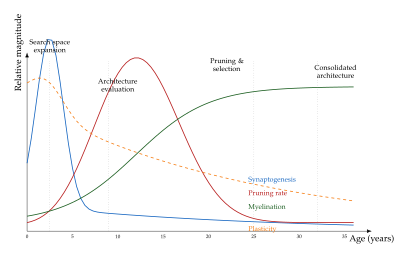
Then something remarkable happens. The brain begins to prune. Connections that are reinforced by repeated experience grow stronger; those that languish without stimulation are systematically eliminated. Between the ages of two and sixteen, roughly half of all synapses are removed in a process that neuroscientists call synaptic pruning. The mature adult brain, far from being a static organ, is the carefully sculpted product of a two-phase process: first, a dramatic over-expansion of connectivity; then, a prolonged period of experience-driven refinement.
The detective's first question is immediate and pointed: why would evolution favour such a seemingly wasteful strategy? Why build a massively over-connected network only to dismantle half of it? And if nature's approach to building intelligence involves searching through a vast space of possible wiring diagrams and pruning towards an optimal one, does this tell us something fundamental about how we should design neural network architectures for artificial intelligence?
This chapter argues that the answer is yes. The biological brain's developmental programme is, in a precise mathematical sense, a neural architecture search algorithm, one that has been refined by hundreds of millions of years of evolutionary pressure. Understanding this biological algorithm will illuminate the principles behind modern computational approaches to architecture search, and will reveal deep connections between neuroscience, information theory, and the mathematics of optimisation.
We begin where all good detective stories begin: at the scene of creation itself.
From Baseline to Blueprint: Cortical Development
The construction of the human brain proceeds in phases that bear a striking resemblance to the stages of a well-designed engineering project. The genetic programme encoded in DNA provides what we might call the initial search space: a set of instructions that specify the broad architecture (how many neurons to produce, their general types, the rough layout of cortical regions) without dictating every last connection. This genetic blueprint is remarkably compact. The human genome contains approximately three billion base pairs, encoding roughly twenty thousand protein-coding genes, yet it must specify a brain with neurons and synapses. The genome cannot possibly encode each connection individually; instead, it specifies rules for generating and refining connectivity, much as a procedural graphics algorithm specifies rules for generating complex textures rather than storing each pixel.
Definition 1 (Neural Search Space).
The biological neural search space is the set of all possible wiring configurations (graphs) that can arise from a given genetic programme . Formally, let denote a set of neurons and a set of directed synaptic connections with associated weights . Then The size of this space is astronomically large: with neurons, the number of possible directed graphs is , a number that dwarfs the number of atoms in the observable universe ().
Prenatal development: building the hardware.
During the first trimester of gestation, neural progenitor cells in the embryonic neural tube divide at an extraordinary rate, producing roughly new neurons per minute at peak neurogenesis [57]. These neurons then migrate along radial glial fibres to their designated positions in the developing cortex, a journey that can span several millimetres (an enormous distance at the cellular scale). The migration is guided by chemical gradients (chemoattractants and chemorepellents) that act as a coarse-grained positioning system. By the end of the second trimester, the vast majority of cortical neurons have reached their final positions, and the basic laminar structure of the six-layered neocortex is established.
At this stage, the brain resembles an enormous collection of components that have been placed on a circuit board but not yet soldered together. The neurons are present, but the synaptic connections between them are sparse. Axons have begun to extend towards their target regions, guided by molecular signalling pathways, but the fine-grained wiring remains to be determined.
Postnatal synaptogenesis: exploring the search space.
Birth triggers a dramatic acceleration of connectivity. Freed from the metabolically constrained intrauterine environment and exposed to the rich sensory world, the infant brain enters a phase of explosive synaptogenesis: the formation of new synaptic connections. In the visual cortex, synaptic density increases from approximately synapses per neuron at birth to roughly per neuron by age two, a six-fold increase driven primarily by experience [58].
This expansion is not random. Neurons that are activated by sensory input extend new dendritic spines (the postsynaptic structures that receive signals from other neurons) and form connections preferentially with neurons that are co-activated. The result is a rapid, experience-driven exploration of the connectivity space: the brain is “trying out” many possible wiring configurations simultaneously, allowing the statistics of the sensory environment to guide which connections are formed.
Critical periods: windows of architectural plasticity.
Not all brain regions undergo synaptogenesis and pruning on the same schedule. Critical periods are developmental windows during which specific brain circuits exhibit heightened plasticity, the capacity for structural and functional reorganisation. The critical period for binocular vision, for example, peaks between ages one and five; during this window, abnormal visual input (such as a misaligned eye) can cause permanent rewiring of the visual cortex. The critical period for native language acquisition extends roughly from birth to age seven [59], after which acquiring native-level phonological distinctions becomes dramatically more difficult.
Recent longitudinal neuroimaging studies have revealed that brain development continues far longer than the traditional view suggested. While early textbooks placed the end of major brain development at approximately age twenty-five, large-scale studies tracking thousands of individuals have shown that significant structural remodelling continues through the early thirties [60]. The period from approximately age nine to age thirty-two is characterised by continuous rewiring: cortical thickness decreases (reflecting ongoing pruning), white matter integrity increases (reflecting myelination of frequently used pathways), and the balance between excitatory and inhibitory neurotransmission gradually shifts towards greater inhibitory control. After approximately age thirty-two, the brain shifts from active restructuring to consolidation, locking in the pathways that have been most frequently and successfully used.
Historical Note.
The story of how we came to understand the brain as a network of individual neurons is itself a remarkable detective story. In the late nineteenth century, the Italian physician Camillo Golgi developed a silver staining technique that made individual neurons visible under the microscope for the first time. The Spanish anatomist Santiago Ramón y Cajal used Golgi's own technique to argue, against Golgi's own belief, that the nervous system was composed of discrete cells (the “neuron doctrine”) rather than a continuous reticulum [1]. Cajal's exquisite drawings of neural circuits, produced entirely by hand from microscope observations, remain among the most beautiful scientific illustrations ever created. Golgi and Cajal shared the 1906 Nobel Prize in Physiology or Medicine, despite holding diametrically opposed views about the very nature of the nervous system.
Half a century later, the Canadian psychologist Donald Hebb proposed a learning rule that would become the foundation of both neuroscience and artificial neural networks: “When an axon of cell A is near enough to excite a cell B and repeatedly or persistently takes part in firing it, some growth process or metabolic change takes place in one or both cells such that A's efficiency, as one of the cells firing B, is increased” [2]. This principle, often summarised as “cells that fire together wire together,” provided the first mechanistic account of how experience could modify brain structure. Hebb's rule is, in essence, a local architecture search algorithm: connections that participate in successful computations are strengthened, while those that do not are weakened and eventually pruned.
Synaptic Pruning: Nature's Architecture Search
The over-connected infant brain faces a fundamental problem: it has too many parameters. With approximately synapses, the network is massively over-parameterised relative to the structure of the sensory world it must model. The solution that evolution has converged upon is elegant and, as we shall see, deeply relevant to modern neural architecture search: the brain performs experience-dependent pruning, systematically eliminating connections that do not contribute to useful computation.
The mechanism is straightforward in principle. When a presynaptic neuron fires and the postsynaptic neuron is subsequently activated, the synapse connecting them is strengthened, a phenomenon called long-term potentiation (LTP). Conversely, when the firing of neuron consistently fails to contribute to the activation of neuron , the synapse is weakened through long-term depression (LTD) and may eventually be eliminated entirely. The result is a use-it-or-lose-it dynamic in which the statistics of the environment sculpt the network's architecture.
Definition 2 (Hebbian Learning Rule).
Let denote the activation of neuron at time , and let denote the synaptic weight from neuron to neuron . The Hebbian learning rule updates the weight according to (HEBB RULE) where is the learning rate. When both neurons are simultaneously active ( and ), the weight increases; when either is silent, the weight remains unchanged. In the continuous-time limit, this becomes (HEBB Continuous) where the decay term prevents unbounded weight growth and implements a form of synaptic homeostasis.
The Hebbian rule in (HEBB RULE) has a well-known instability: weights can grow without bound when neurons are persistently co-activated. The biological brain addresses this through several homeostatic mechanisms, including synaptic scaling (a global multiplicative normalisation of all synapses on a given neuron) and metaplasticity (the plasticity threshold itself shifts depending on recent activity). These mechanisms ensure that the total synaptic drive to each neuron remains within a functional range, preventing runaway excitation.
Proposition 1 (Hebbian Pruning Dynamics).
Consider a network of neurons with weight matrix evolving under the regularised Hebbian rule in (HEBB Continuous). Let denote the input correlation matrix, assumed to be positive semidefinite with eigenvalues . Then the equilibrium weight matrix satisfies and synapses corresponding to weakly correlated neuron pairs (small entries of ) converge to near-zero weights and are candidates for pruning. Specifically, a synapse satisfies for pruning threshold whenever
Proof.
At equilibrium, , so from (HEBB Continuous), Solving for gives . In matrix form, . The pruning condition follows directly: if and only if , which gives .
Proposition 1 reveals a deep principle: Hebbian learning, combined with weight decay, naturally identifies synapses that carry little statistical information about the correlational structure of the environment. These are precisely the synapses that the brain prunes. The pruning threshold plays the role of a significance level: only connections whose correlation exceeds a minimum strength survive.
The pruning timeline.
Synaptic pruning is not a single event but a protracted process that unfolds over more than a decade. In the visual cortex, pruning begins around age one and reaches a plateau by puberty. In the prefrontal cortex, which governs executive function, planning, and impulse control, pruning continues into the mid-twenties and possibly beyond. The total reduction is substantial: approximately of synapses are eliminated between peak density (age two to three) and adulthood [58].
This prolonged timeline is not a design flaw; it reflects the different timescales on which different brain regions must adapt to their inputs. The visual cortex, which processes relatively low-level features (edges, colours, motion), can converge on an efficient architecture quickly because the statistics of visual input are relatively stable. The prefrontal cortex, which must learn complex social rules, abstract reasoning strategies, and long-horizon planning, requires a longer search period because the relevant “training data” arrives slowly over years of social and cognitive experience.
Definition 3 (Synaptic Plasticity Rate).
The synaptic plasticity rate quantifies the capacity for structural change in a neural circuit as a function of developmental time (measured in years from birth). We model it as a decaying exponential with a nonzero baseline: (Plasticity RATE) where is the peak plasticity at birth, is the plasticity decay rate, and is the residual adult plasticity. Empirical estimates suggest (normalised units), , and , indicating that even in adulthood, the brain retains approximately of its peak capacity for structural reorganisation.
The plasticity rate governs the effective “learning rate” for architectural changes. During critical periods, is high, and the network can rapidly rewire in response to experience. As declines, architectural changes become slower and more incremental, eventually reaching the baseline level that supports lifelong learning at a reduced rate. This mirrors a common strategy in neural architecture search: begin with aggressive exploration (high architectural learning rate), then gradually reduce the rate of structural changes as the search converges, a form of simulated annealing applied to network topology.
Key Idea.
The brain does not design its architecture from a blank slate. Instead, it follows a two-phase strategy: (1) grow an over-parameterised network with far more connections than ultimately needed, then (2) prune away connections that are not reinforced by experience. This “grow then prune” strategy has a deep computational rationale: the initial over-expansion ensures that no potentially useful connection is missed, while the subsequent pruning removes the noise and converges to an efficient architecture matched to the environment. This is the biological analog of architecture pruning in neural architecture search, and it suggests that the NAS community's interest in pruning-based methods is not merely a computational convenience but a recapitulation of a strategy refined by hundreds of millions of years of evolution.
Two complementary strategies.
The brain's “grow then prune” approach is not the only possible strategy. An alternative is “start simple and grow”: begin with a minimal architecture and progressively add capacity as needed. Both strategies exist in the NAS literature. Pruning-based approaches (such as network slimming and lottery ticket methods [61]) follow the biological model, starting with a large network and removing unnecessary components. Progressive growing approaches (such as Net2Net [62] and progressive growing of GANs [63]) follow the alternative model, starting small and adding capacity incrementally.
Which strategy is better? The answer depends on the prior knowledge available. When the target architecture is believed to be a subset of a known large architecture, pruning is efficient because the search space is implicitly defined by the parent network. When the target architecture may require novel structural motifs not present in any initial design, progressive growing is more flexible because it can explore regions of the search space that pruning alone cannot reach. The brain uses both: synaptogenesis (growing) and pruning (shrinking) occur simultaneously during development, with the balance shifting from growth-dominated to pruning-dominated as the organism matures.
Lifelong learning: growth or rewiring?
A natural question arises: do adult brains continue to grow new neurons, or do they primarily rewire existing connections? The answer, established through decades of research, is nuanced. Adult neurogenesis (the birth of new neurons) occurs in a few restricted brain regions, most notably the hippocampus (involved in memory formation) and the olfactory bulb (involved in smell processing) [64]. However, the rate of adult neurogenesis is low compared to developmental neurogenesis, and its functional significance remains debated.
The dominant mode of adult brain plasticity is rewiring: existing synapses are strengthened, weakened, or eliminated, and new synapses can form between existing neurons. This rewiring comes at a cost: strengthening one set of connections often entails weakening others, a phenomenon that manifests as forgetting. The brain manages this tradeoff through consolidation mechanisms (which we will explore in Sleep, Dreams, and Offline Consolidation) that protect important memories while allowing less critical ones to fade. The implication for artificial systems is significant: adaptive networks that modify their architecture during deployment must contend with the same stability-plasticity tradeoff that the brain faces.
What Limits Growth? Physical and Computational Constraints
The brain is not free to grow without bound. It operates under a stringent set of physical, metabolic, and computational constraints that fundamentally shape its architecture. Understanding these constraints illuminates why the brain looks the way it does, and, more importantly, provides a framework for understanding the analogous constraints that govern artificial neural network design.
Metabolic cost.
The human brain accounts for approximately of body mass but consumes roughly of the body's resting metabolic energy, a disproportionate share that reflects the extraordinary energy demands of neural computation [65]. Each neuron consumes energy to maintain its resting membrane potential, to propagate action potentials along its axon, and to release and recycle neurotransmitters at synaptic junctions. The energy cost per synaptic event has been estimated at approximately ATP molecules, corresponding to roughly joules ( picojoule) per synaptic transmission. At a firing rate of Hz and with synapses per neuron, each active neuron consumes on the order of W at peak. Because only a small fraction of the brain's neurons fire at any instant (sparse coding), the whole brain empirically consumes only about W, far below the W that a continuously firing population would demand.
Proposition 2 (Metabolic Bound on Network Size).
Let denote the average power consumption per neuron (in watts), and let denote the total energy budget available for neural computation (in watts). Then the maximum number of neurons that can be sustained is bounded by (Metabolic Bound) For the human brain, W (accounting for the fact that not all neurons fire at maximum rate simultaneously; the average power per neuron, including maintenance costs, is lower than the peak per-spike cost) and W, yielding This bound is consistent with the observed neuron count of approximately (the discrepancy reflects the fact that glial cells and other support structures share the energy budget).
Proof.
The proof follows directly from energy conservation. If each of neurons consumes power simultaneously, the total power consumption is . For the brain to operate within its energy budget, we require , which gives . The bound is tight when all neurons are active simultaneously, which occurs approximately during wakefulness when large-scale neural populations are engaged in coordinated processing. In practice, not all neurons fire simultaneously, so the effective bound is somewhat higher than computed at peak per-neuron rates, but the order of magnitude is correct.
Cranial volume constraints.
The skull imposes a hard upper bound on brain volume. The average adult human cranial capacity is approximately cm, and this volume must accommodate not only neurons but also glial cells (which outnumber neurons by a factor of roughly one to one in humans), blood vessels (the brain receives approximately of cardiac output), cerebrospinal fluid, and the meninges. The packing density of neurons in the cortex is approximately neurons per mm, and this density cannot be increased arbitrarily without compromising the space available for axons, dendrites, and supporting vasculature.
Wiring optimisation.
Axons, the long projections through which neurons transmit signals to distant targets, occupy physical space and consume metabolic resources proportional to their length. The brain's wiring problem is analogous to a VLSI circuit layout problem: given a set of functional units (cortical regions) and a set of required connections (white matter tracts), find an arrangement that minimises total wire length while satisfying all connectivity constraints [66]. This optimisation shapes the brain's physical layout: functionally related regions tend to be physically adjacent (minimising short-range wiring), while long-range connections (such as the corpus callosum connecting the two hemispheres) are reserved for communication that cannot be achieved through local circuits alone.
Proposition 3 (Wiring Length Minimisation).
Consider a network of neurons with positions and a required connectivity pattern specified by an adjacency matrix . The total wiring length is (Wiring Length) The optimal placement problem is NP-hard in general (by reduction from the quadratic assignment problem). However, spectral relaxation provides an approximate solution: the optimal positions are related to the leading eigenvectors of the graph Laplacian , where . Specifically, the eigenvectors corresponding to the second through fourth smallest eigenvalues of provide a three-dimensional embedding that approximately minimises total wiring length.
Proof.
We sketch the proof. The wiring length objective involves norms, which makes the problem non-smooth. Replacing with (the squared Euclidean distance) gives a smooth relaxation. Let be the matrix whose -th row is . Then the squared wiring length can be written as Minimising subject to (to prevent the trivial solution ) is a Rayleigh quotient problem. By the Courant-Fischer theorem, the minimum is achieved when the columns of are the eigenvectors corresponding to the smallest eigenvalues of . The smallest eigenvalue is always zero (with eigenvector , corresponding to a constant translation), so the nontrivial solution uses eigenvectors . The NP-hardness of the original () problem follows from the known NP-hardness of the quadratic assignment problem [3].
Insight.
Physical constraints in biology parallel compute, memory, and latency constraints in hardware-aware neural architecture search. The brain is, in a very real sense, the ultimate hardware-aware architecture: it has been optimised not only for computational performance but also for energy efficiency, physical compactness, and communication bandwidth. Every modern hardware-aware NAS algorithm that jointly optimises accuracy and latency is, perhaps unknowingly, following the same multi-objective optimisation strategy that evolution has employed for hundreds of millions of years.
| Biological Constraint | NAS Analog | Typical Metric |
| Metabolic cost (20 W) | Computational cost | FLOPs, MACs |
| Cranial volume (1400 cm) | Memory budget | GPU RAM (GB) |
| Axonal wiring length | Communication latency | Inference latency (ms) |
| Synaptic density limit | Parameter count | # Parameters |
| Heat dissipation | Thermal design power | TDP (watts) |
| Blood supply bandwidth | Memory bandwidth | GB/s |
| Neurotransmitter recycling rate | Batch throughput | Samples/second |
| Developmental time | Training time | GPU-hours |
Exercise 1.
Energy efficiency of biological vs. artificial networks. The human brain performs approximately synaptic operations per second while consuming W, yielding an energy efficiency of operations per watt. A modern GPU (such as the NVIDIA H100) performs approximately FLOPs while consuming W, yielding approximately operations per watt. (a) Compute the ratio of biological to artificial energy efficiency. (b) If hardware energy efficiency improves at a rate of every years (a generous interpretation of Moore's law for energy), how many years until artificial hardware matches biological energy efficiency? (c) Discuss why this comparison is imprecise (hint: consider the difference between a synaptic operation and a floating-point operation).
Exercise 2.
Spectral neuron placement. Consider a network of neurons arranged in a ring graph (neuron connected to neurons and modulo ). (a) Write down the adjacency matrix and the graph Laplacian . (b) Compute the eigenvalues and eigenvectors of . (c) Using the second and third eigenvectors, embed the neurons in . Verify that the resulting layout places the neurons approximately on a circle, confirming that the spectral method recovers the natural ring geometry.
The Information-Theoretic Brain
If the brain is an architecture search algorithm, refined by evolution and fine-tuned by experience, then what are its fundamental limits? What determines the maximum amount of information a neural circuit can process, and how does this constrain the architectures that can emerge from the developmental search? To answer these questions, we turn to the language of information theory, the mathematical framework that Claude Shannon developed in 1948 to quantify the fundamental limits of communication [67].
The application of information theory to neuroscience is not merely an analogy. Neurons are, quite literally, communication channels: they receive input signals (via dendrites), perform a nonlinear computation (in the cell body), and transmit the result (via action potentials along the axon) to downstream neurons. The reliability, capacity, and efficiency of this neural communication system are governed by the same mathematical laws that govern telephone lines, fibre optic cables, and wireless networks. Understanding these laws will reveal why certain brain architectures are more efficient than others, and will provide principled bounds on the architectures that neural architecture search should target.
Channel Capacity of Biological Neurons
The neuron as a noisy channel.
A biological neuron receives input from hundreds to thousands of presynaptic neurons, integrates these signals, and produces an output in the form of a sequence of electrical impulses called action potentials or spikes. The spike is an all-or-nothing event: it either occurs or it does not, with a relatively stereotyped waveform. The information carried by a neuron is therefore encoded not in the shape of individual spikes (which is approximately constant) but in the timing and rate of spikes.
Two principal coding schemes have been identified in the neuroscience literature. In rate coding, the information is carried by the average firing rate over some time window : a higher rate indicates a stronger response. In temporal coding, the information is carried by the precise timing of individual spikes relative to some reference (such as the phase of an ongoing oscillation or the timing of spikes in other neurons). The distinction between these coding schemes has profound implications for neural channel capacity, as temporal coding can in principle carry far more information per spike than rate coding.
Definition 4 (Neural Channel Capacity).
Consider a single neuron as a discrete memoryless channel with input (the input spike train from presynaptic neurons) and output (the output spike train). The neural channel capacity is (Neural Channel Capacity) where is the mutual information between input and output, is the entropy of the output, and is the conditional entropy of the output given the input (the “noise entropy”). The maximum is taken over all possible input distributions consistent with the neuron's biophysical constraints (maximum firing rate, refractory period, energy budget).
Experimental measurements of neural channel capacity, performed by recording the responses of individual neurons to repeated presentations of the same stimulus, have yielded estimates in the range of to bits per spike, depending on the neuron type and the coding scheme employed [68]. Neurons in the fly visual system, which use precise temporal coding, achieve the upper end of this range (– bits per spike). Cortical neurons in mammals, which tend to rely more heavily on rate coding, typically achieve lower information rates (– bits per spike).
Example 1.
Channel capacity of a rate-coding neuron. Consider a neuron that encodes information via its firing rate over a time window ms. Suppose the neuron can fire at rates between Hz and Hz, and that the observed rate is corrupted by Gaussian noise with standard deviation Hz. Under rate coding, the output is effectively a continuous variable where . The channel capacity for a Gaussian channel with input power constraint and noise variance is If we model the input as uniformly distributed over , the signal variance is Hz, and the capacity is Over the ms window, this corresponds to an information rate of approximately bits per second. With rate-coding neurons operating in parallel, the aggregate information rate is bits/s kbps.
Total information throughput of the brain.
With approximately neurons, each firing at an average rate of perhaps – Hz and carrying – bits per spike, the theoretical maximum information throughput of the human brain is enormous: on the order of to bits per second. However, the useful information rate, the rate at which the brain extracts and processes behaviourally relevant information from its sensory input, is vastly lower. Estimates of the conscious information processing rate range from to bits per second [69], while the visual cortex is estimated to process approximately bits per second of visual information.
Remark 1.
The enormous gap between the brain's theoretical channel capacity (– bits/s) and its useful information processing rate (– bits/s) is not a sign of inefficiency but a reflection of massive redundancy and error correction. Much of the brain's neural activity is devoted to internal communication, homeostatic regulation, prediction, and noise suppression rather than to processing external information. This gap parallels the well-known observation in deep learning that the number of parameters in a neural network (its “raw capacity”) vastly exceeds the effective number of parameters (its “useful capacity”) as measured by the information stored about the training set. In both biological and artificial systems, the gap between raw and effective capacity reflects the cost of robustness.
Connection to rate-distortion theory.
The brain's sensory processing can be viewed through the lens of rate-distortion theory, which characterises the minimum number of bits needed to represent a source signal at a given level of fidelity. The rate-distortion function gives the minimum mutual information between the source and its compressed representation that is achievable at distortion level : (RATE Distortion) where is a distortion measure. The visual cortex performs a form of lossy compression: it extracts the features of the visual scene that are most relevant for behaviour (object identity, spatial layout, motion) while discarding details that are less behaviourally relevant (exact pixel intensities, fine texture details). This compression is adaptive: the features that are preserved depend on the task at hand (recognising a face vs. navigating a cluttered room vs. tracking a moving prey).
Proposition 4 (Capacity-Distortion Tradeoff for Neural Representations).
Let be a continuous sensory input with differential entropy , and let be a neural representation of with at most bits of capacity. Then the minimum achievable expected distortion under squared-error loss satisfies (Capacity Distortion) which is the Shannon lower bound. Equality holds when is Gaussian. This bound implies that reducing distortion by a factor of requires increasing the representation capacity by bit (since ).
Proof.
For a continuous source with differential entropy and squared-error distortion , the rate-distortion function satisfies (the Shannon lower bound). Setting (the capacity constraint) and solving for gives For Gaussian , , and the rate-distortion function is for , achieving the lower bound with equality.
The Information Bottleneck in Neural Systems
The rate-distortion framework tells us how much information we need to retain about the input to achieve a given level of fidelity. But in most learning problems, we do not care about reconstructing the input perfectly; we care about predicting a target variable from the input . The relevant question is not “how much information about should we retain?” but rather “which information about should we retain?” This distinction leads to one of the most influential ideas in modern learning theory: the information bottleneck principle.
Theorem 1 (Information Bottleneck).
Let be an input random variable, a target random variable jointly distributed with , and a compressed representation of . The information bottleneck (IB) objective [4] seeks a representation that retains maximal information about while compressing as much as possible: (IB Objective) where is a Lagrange multiplier controlling the tradeoff between compression () and prediction (). The optimal encoder satisfies the self-consistent equations: (IB Encoder) where is a normalising constant, and denotes the Kullback-Leibler divergence.
Proof.
We derive the self-consistent equations using the method of Lagrange multipliers. The IB objective is We must also enforce the normalisation constraint for all . Adding Lagrange multipliers for these constraints and taking the functional derivative with respect to : Setting this to zero and noting that (up to a term that does not depend on ), we obtain where the constant absorbs terms independent of . Exponentiating both sides: where ensures normalisation. Equations and follow from the definitions of the marginal and the Bayes-optimal decoder, respectively. The three equations are coupled (each depends on the others), and the solution is obtained by alternating iterations [4].
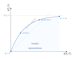
The information bottleneck has a beautiful geometric interpretation. As varies from to , the optimal representation traces a curve in the plane called the information curve. At , the representation carries no information about either or (total compression). As increases, the representation captures progressively more information about , at the cost of retaining more information about . In the limit , compression is not penalised, and retains all information about that contains (i.e., ).
Connection to deep learning.
Shwartz-Ziv and Tishby [70] proposed that the layers of a deep neural network can be viewed as successive information bottlenecks: each layer compresses the representation from the previous layer while (ideally) preserving information about the target . Their empirical analysis of fully connected networks trained on simple classification tasks revealed a striking two-phase training dynamic. During the initial “fitting” phase, the mutual information increases rapidly as the network learns to predict the target. During the subsequent “compression” phase, decreases as the network learns to discard input information that is not relevant to prediction.
This two-phase dynamic mirrors the brain's developmental trajectory: the early synaptogenesis phase (expanding connectivity to capture information about the environment) corresponds to the fitting phase, while the subsequent pruning phase (eliminating connections that carry noise rather than signal) corresponds to the compression phase.
Remark 2.
The information bottleneck interpretation of deep learning has been the subject of significant debate. Saxe et al. [5] showed that the compression phase observed by Shwartz-Ziv and Tishby depends on the choice of activation function: networks with saturating nonlinearities (such as ) exhibit compression, while networks with non-saturating nonlinearities (such as ReLU) do not. Furthermore, estimating mutual information in high dimensions is notoriously difficult, and the precise values reported in information-plane analyses are sensitive to the estimation method used. Despite these caveats, the qualitative insight that neural networks learn by first fitting and then compressing remains influential and has inspired compression-based approaches to neural architecture search.
Remark 3.
Does the information bottleneck explain why the brain prunes synapses? Consider a synapse that carries mutual information primarily with noise in the input rather than with the target signal. In information-theoretic terms, this synapse contributes to without contributing to . Eliminating such a synapse reduces (compression) while leaving (prediction) largely unchanged, moving the representation towards the optimal point on the information bottleneck curve. Synaptic pruning can thus be interpreted as a biological implementation of information bottleneck compression: the brain identifies and removes neural pathways that carry task-irrelevant information, converging towards a representation that is maximally compressed while retaining maximum predictive power.
Information-Theoretic Limits on Architecture Size
The information bottleneck tells us what information an optimal representation should retain. But it does not directly tell us how large the architecture implementing that representation must be. How many parameters does a network need to achieve a given level of predictive performance? And can a network be too large?
These questions lie at the intersection of information theory and statistical learning theory, and the answers have direct implications for neural architecture search: they define the target region in the space of architecture sizes that NAS should aim for.
Minimum description length and architecture selection.
The minimum description length (MDL) principle provides a natural framework for architecture selection. MDL states that the best model for a dataset is the one that minimises the total description length: the number of bits needed to describe the model plus the number of bits needed to describe the data given the model: (MDL) where is the description length of architecture (proportional to the number of parameters if each parameter requires a fixed number of bits to specify), and is the description length of the data given the model (related to the negative log-likelihood of the data under the model's best-fit parameters).
Too small an architecture results in high data cost (underfitting): the model cannot capture the structure in the data, so the residuals require many bits to describe. Too large an architecture results in high model cost (overfitting): the model has many parameters, most of which encode noise rather than signal. The MDL-optimal architecture balances these two costs.
Theorem 2 (Architecture Capacity Bound).
Consider a supervised learning task with i.i.d. samples drawn from a joint distribution on . Let denote the hypothesis class induced by architecture with effective parameters, where each parameter has capacity at most bits (i.e., each parameter can represent at most distinct values after quantisation). Then, for the excess risk to be achievable, the effective architecture size must satisfy (Capacity Bound)
Proof.
The proof proceeds via a counting argument. An architecture with parameters, each with capacity bits, can represent at most distinct hypotheses. For the hypothesis class to achieve excess risk on samples from a distribution with conditional entropy , it must be able to distinguish between at least distinct input-output patterns (this follows from Fano's inequality: the probability of error in predicting from is bounded below by a function of the conditional entropy and the number of hypotheses available).
Specifically, by Fano's inequality, for the average probability of error to satisfy , we need the mutual information between the data and the hypothesis to be at least where is the binary entropy. For small , the last two terms are , and the dominant term is .
Since the mutual information between the data and the hypothesis is bounded by the capacity of the hypothesis class, , we obtain and rearranging (absorbing lower-order terms into the denominator) yields the stated bound.
Definition 5 (Effective Parameter Count).
The effective parameter count of an architecture with nominal parameter count is the minimum number of parameters needed to specify a hypothesis in to within a precision sufficient for achieving a target excess risk . Formally, (Effective Params) where is the -covering number of the hypothesis class (the minimum number of hypotheses needed to cover the class at resolution ). In practice, for overparameterised networks, reflecting the low intrinsic dimensionality of the learned representation.
PAC-Bayes bounds and architecture priors.
The PAC-Bayes framework provides another information-theoretic lens on architecture selection. A PAC-Bayes bound states that, with probability at least over the draw of training samples, for any posterior distribution over hypotheses, (PAC Bayes) where is the true risk, is the empirical risk, and is a prior distribution over hypotheses chosen before seeing the data. The key quantity is the KL divergence : the “surprise” of the posterior relative to the prior.
When applied to architecture search, the prior is a distribution over architectures (and their parameters), and the KL term penalises architectures that deviate significantly from prior expectations. A well-chosen prior, informed by domain knowledge or by the structure of previously successful architectures, can dramatically tighten the bound and guide the search towards architectures with strong generalisation guarantees.
Proposition 5 (PAC-Bayes Architecture Selection).
Let be a finite set of candidate architectures, and let be a prior probability over architectures satisfying . For each architecture , let and be the prior and posterior over parameters, respectively. Then the PAC-Bayes bound for the architecture selection problem is: with probability , (PAC Bayes ARCH) for any architecture and any posterior over its parameters. The term penalises architectures with low prior probability, favouring simpler or more “expected” designs.
Proof.
Apply the standard PAC-Bayes theorem ((PAC Bayes)) with the combined prior over architecture-parameter pairs. For a specific architecture with posterior over parameters, the KL divergence decomposes as since is supported entirely on architecture . Substituting into the PAC-Bayes bound yields the result.
Caution.
Larger networks can memorise the training data but may not generalise. The information bottleneck principle suggests that there exists an optimal architecture size for each task: neither too small (leading to underfitting and high distortion) nor too large (leading to overfitting and wasted capacity). This optimal size depends on the task's intrinsic dimensionality: the number of independent factors of variation in the data-generating process. A task with low intrinsic dimensionality (e.g., recognising handwritten digits, which can be described by a few stroke parameters) requires a smaller architecture than a task with high intrinsic dimensionality (e.g., generating photorealistic images, which requires modelling texture, lighting, geometry, and semantics simultaneously). Neural architecture search should target architectures near this optimal size, not simply maximise parameter count.
| Quantity | Role in Architecture Sizing |
| Irreducible noise; sets the lower bound on achievable loss regardless of architecture | |
| Total learnable information; upper bounds the useful capacity the architecture must provide | |
| Representation complexity; should be minimised subject to preserving | |
| Prediction quality; should be maximised subject to compression constraints | |
| Per-parameter capacity; depends on numerical precision (float32: 23 bits mantissa) | |
| Effective architecture size; the actual “useful” parameter count | |
| PAC-Bayes complexity; penalises deviation from prior architecture expectations |
Exercise 3.
Gaussian information bottleneck. Consider the jointly Gaussian case: and where is independent of . (a) Compute . (b) Show that the optimal IB representation is where for an appropriate choice of depending on . (c) Derive the IB curve as a function of and verify it is concave. (d) Find the value of at which the IB solution transitions from being independent of to carrying information about (the “phase transition”).
Exercise 4.
MDL for polynomial regression. Consider fitting a polynomial of degree to data points generated from with and uniformly sampled from . (a) For each degree , compute the MDL criterion: model cost bits (assuming float32 parameters) plus data cost where is the least-squares fit. (b) Plot the total MDL as a function of and identify the optimal degree . (c) Compare with the degree selected by -fold cross-validation.
Challenge 1.
PAC-Bayes-guided architecture search. Design a simple architecture search algorithm that uses the PAC-Bayes bound in (PAC Bayes ARCH) as its objective. Consider a search space of fully connected networks with hidden layers, each with width . (a) Define a prior over the possible architectures (hint: use a prior that favours smaller networks). (b) For each architecture, train the network on a simple classification task (e.g., MNIST) and compute the PAC-Bayes bound using a Gaussian posterior centred on the trained weights. (c) Select the architecture that minimises the bound. (d) Compare with the architecture selected by validation accuracy. Do the two criteria agree?
From Brains to Machines: The Adaptive Network Hypothesis
We have established that nature builds brains through a remarkable process of expansion, evaluation, and pruning, subject to stringent physical and information-theoretic constraints. The infant brain generates a massively over-connected network, tests each connection against the statistics of the environment, and eliminates those that do not earn their metabolic keep. The resulting architecture is not designed from first principles but discovered through a search process that combines genetic priors with experiential refinement.
The central question of this chapter crystallises: Can we engineer the same process for artificial neural networks? Can we build systems that do not merely learn better weights for a fixed architecture but learn the architecture itself, adapting their structure to the task at hand? And can we do this efficiently enough to be practical, compressing the biological search that unfolds over years of development (and millions of years of evolution) into hours or days of computation?
Can Neural Networks Grow New Neurons?
Biological neurogenesis revisited.
In the adult brain, the birth of new neurons (neurogenesis) is highly restricted. The two primary sites of adult neurogenesis are the subgranular zone of the hippocampal dentate gyrus (where new neurons contribute to memory formation) and the subventricular zone lining the lateral ventricles (where new neurons migrate to the olfactory bulb) [64]. The rate of hippocampal neurogenesis in humans has been estimated at approximately new neurons per day in each hippocampus, a small number compared to the hippocampus's roughly million existing neurons.
The limited scope of adult neurogenesis means that the brain's primary mode of adaptation in adulthood is rewiring rather than growth: existing connections are strengthened, weakened, or eliminated, and new synapses can form between existing neurons, but the addition of entirely new computational units is rare. This rewiring comes at a cost: strengthening connections in one circuit often requires weakening connections in others, a phenomenon that manifests as the familiar experience of forgetting. The brain manages this tradeoff through sophisticated consolidation mechanisms that protect important memories while allowing less critical ones to fade, a theme we will return to in Sleep, Dreams, and Offline Consolidation.
Artificial analogs: dynamic network expansion.
Several approaches in the machine learning literature mirror different aspects of biological network growth.
Definition 6 (Function-Preserving Network Expansion).
A function-preserving network expansion transforms a trained network with architecture into a larger network with architecture such that (Function Preserving) The expanded network has strictly more parameters than the original () but computes exactly the same function at initialisation. Subsequent training of can then explore the enlarged capacity of the new architecture.
Chen et al. [62] introduced two specific operators for function-preserving expansion. The Net2WiderNet operator adds neurons to a hidden layer by cloning an existing neuron and splitting its outgoing weights by a factor of two, so that the summed contribution to the next layer is unchanged. The Net2DeeperNet operator adds a new layer initialised as the identity function (for fully connected layers, ; for convolutional layers, a identity filter), so that the network's input-output mapping is preserved.
Proposition 6 (Net2WiderNet Preserves Function).
Let be a network with a hidden layer of width with weight matrices (input to hidden) and (hidden to output), and let denote the element-wise activation function. The Net2WiderNet operation replaces the hidden layer with width by choosing an index and setting: (Net2wider W1) Then for all .
Proof.
Let be the hidden activations. The output of the original network is . After the Net2WiderNet operation, the new hidden activations are , where is the activation of the cloned neuron (identical to the -th original activation since ). The new output is
Progressive growing.
An alternative to expanding a trained network is to build the architecture progressively from scratch. Karras et al. [63] demonstrated this approach dramatically in the context of generative adversarial networks (GANs): both the generator and discriminator start as simple networks that produce and evaluate pixel images, and new layers are added incrementally to handle progressively higher resolutions (, , and so on up to ). Each new layer is “faded in” using a learned blending parameter that smoothly interpolates between the output of the previous (lower-resolution) layer and the new (higher-resolution) layer, preventing sudden disruptions to the training dynamics.
Definition 7 (Adaptive Network).
An adaptive network is a neural network in which both the parameters and the architecture evolve during or between training phases. Formally, the evolution is governed by a joint dynamical system: (Adaptive Theta) where is the parameter learning rate, is the loss function, and is an architecture transition operator that modifies the architecture based on the current parameters and data. Unlike a standard neural network (where is fixed at initialisation and only evolves), an adaptive network permits structural modifications including:
Adding or removing neurons (changing layer widths);
Adding or removing layers (changing network depth);
Changing connectivity patterns (e.g., adding skip connections);
Modifying operation types (e.g., replacing convolutions with attention).
Key Idea.
The central question for this chapter, and for the field of neural architecture search more broadly, is this: Can we build foundation models that adapt their architecture, not just their weights, to new tasks, new domains, and new modalities? The biological brain demonstrates that this is possible in principle: the same basic neural substrate can, through developmental sculpting and lifelong plasticity, produce circuits specialised for vision, language, motor control, social cognition, and abstract reasoning. If the brain can do it, what stops machines? The answer, as we shall see, is not a fundamental impossibility but a collection of computational challenges: the search space is vast, evaluation is expensive, and the interaction between architecture and weights is complex. The remainder of this chapter develops the mathematical tools to address each of these challenges.
Sleep, Dreams, and Offline Consolidation
The brain does not learn only while awake. Some of the most important computational processes in the brain occur during sleep, when the organism is disconnected from sensory input and freed from the demands of real-time behaviour. Understanding sleep's role in neural computation provides unexpected insights for the design of adaptive artificial networks.
Hippocampal replay and memory consolidation.
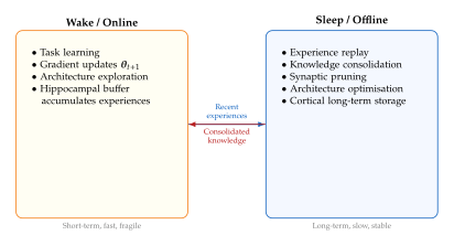
During wakefulness, the hippocampus acts as a rapid learning system, quickly encoding new experiences as patterns of neural activity. These newly formed memories are initially “fragile”: they depend on the specific synaptic connections within the hippocampus and can be disrupted by subsequent learning (new experiences may overwrite the same synaptic connections, causing catastrophic forgetting).
During sleep, particularly during slow-wave (deep) sleep, the hippocampus “replays” recently encoded experiences to the neocortex [71][72]. Place cells in the hippocampus that fired in sequence during spatial navigation, for example, fire in the same sequence during sleep, but at a compressed timescale (approximately – faster than the original experience). This replay is believed to serve several functions:
Memory consolidation: by repeatedly reactivating recent memories, replay strengthens the neocortical representations of these memories, gradually transferring them from hippocampal short-term storage to neocortical long-term storage.
Memory integration: replay allows new memories to be interleaved with older ones, facilitating the discovery of connections and patterns across experiences that were temporally separated.
Synaptic homeostasis: the net effect of replay, combined with global synaptic down-scaling, is to strengthen important connections while weakening unimportant ones, a form of offline architecture optimisation.
The synaptic homeostasis hypothesis.
Tononi and Cirelli [71] proposed the synaptic homeostasis hypothesis (SHY): during wakefulness, learning causes a net increase in synaptic strength across the brain (because Hebbian learning is predominantly potentiating). This net increase has costs: higher energy consumption, reduced signal-to-noise ratio (because all synapses, including noise-carrying ones, are strengthened), and reduced capacity for further learning (because synapses approach their maximum strength). During sleep, a global process of synaptic renormalisation reduces all synaptic strengths proportionally, with one crucial caveat: synapses that have been most strongly potentiated (those carrying the most important information) resist renormalisation more effectively than weakly potentiated synapses. The result is a net pruning effect: weak, noisy connections are driven below the survival threshold and eliminated, while strong, signal-carrying connections survive in a slightly weakened but more energy-efficient form.
We can formalise this process as follows. Let denote the synaptic weight after a period of wakefulness, and let be the global renormalisation factor. The weight after sleep-dependent renormalisation is (Synaptic Renorm) where is a “replay-dependent correction” that is large for synapses involved in replayed memories and small (or zero) for synapses not involved in replay. Synapses with are eliminated. The combined effect of global down-scaling () and selective replay ( for important synapses) implements a form of experience-dependent pruning during offline processing.
Can foundation models “sleep”?
The biological sleep-wake cycle suggests a computational paradigm for adaptive artificial networks. During periods when a deployed foundation model is not actively serving inference requests (or during scheduled maintenance windows), the model could engage in “sleep-like” offline processing:
Replay: revisit important or challenging examples from a stored experience buffer, reinforcing representations that might otherwise decay due to subsequent fine-tuning.
Consolidation: distil knowledge from a large “teacher” model (or from the model's own earlier checkpoints) into a smaller, more efficient “student” architecture, a process analogous to the transfer of memories from hippocampus to neocortex.
Pruning: identify and remove parameters, attention heads, or entire layers that contribute minimally to model performance, reducing the model's computational footprint.
Architecture restructuring: modify the network topology (e.g., adjusting the allocation of layers to different modalities in a multimodal model) based on usage statistics collected during the “wake” phase.
Shetty and others [73] proposed the NeuroDream framework, which implements a sleep-inspired consolidation phase for continual learning. During the “dream” phase, the model generates synthetic examples from its own learned distribution and uses them as additional training data, interleaved with a small buffer of real examples. This self-generated replay serves the same function as hippocampal replay: it reinforces previously learned knowledge without requiring access to the original training data, mitigating catastrophic forgetting.
Remark 4.
The connection between sleep-inspired computation and continual learning is deep. Replay-based continual learning methods, which maintain a buffer of exemplars from previous tasks and interleave them with current-task training data, are computational analogs of hippocampal replay during sleep. Regularisation-based methods, which penalise changes to parameters important for previous tasks (such as Elastic Weight Consolidation; [6]), are analogs of the selective protection of important synapses during sleep-dependent renormalisation. Architectural methods, which allocate different subnetworks to different tasks, are analogs of the brain's strategy of dedicating specialised cortical circuits to different sensory modalities while sharing common computational motifs.
Caution.
Implementing a sleep-like offline phase in production systems carries nontrivial costs. The replay buffer requires storage proportional to the number of experiences retained (with privacy implications if training data is sensitive). The consolidation and pruning phases require compute resources that could otherwise serve inference requests. And the architecture restructuring phase introduces a risk of performance regression if the modifications are poorly calibrated. These costs must be weighed against the benefits of improved efficiency and sustained performance. The biological brain faces an analogous tradeoff: sleep consumes approximately one-third of an organism's life, during which it is vulnerable to predators and unable to forage. The fact that evolution has preserved sleep across virtually all animal species, despite these costs, suggests that the benefits of offline consolidation are substantial.
The Architecture Search Problem: First Formulation
We are now ready to state the neural architecture search problem in its full mathematical generality. The formulation draws on all the threads we have developed: the biological analogy of developmental search, the information-theoretic constraints on architecture size, and the adaptive network hypothesis that architecture and weights should co-evolve.
Definition 8 (Neural Architecture Search Problem).
The neural architecture search (NAS) problem is a bilevel optimisation: (Bilevel) subject to (Inner LOOP) where:
is the search space: the set of all architectures under consideration;
is the neural network with architecture and parameters ;
is the training loss (evaluated on training data);
is the validation loss (evaluated on held-out data, serving as a proxy for generalisation);
denotes the optimal weights for architecture , obtained by solving the inner optimisation problem.
The outer loop searches over architectures; the inner loop, for each candidate architecture, trains the weights to optimality (or an approximation thereof).
The bilevel structure of the NAS problem is both its defining characteristic and its primary computational challenge. The outer loop is a combinatorial (or mixed continuous-discrete) optimisation over the structured space of architectures. The inner loop is a continuous optimisation over weights, which is itself a high-dimensional, non-convex problem that typically requires many gradient descent steps to solve. The coupling between the two levels is what makes NAS fundamentally different from (and harder than) standard hyperparameter optimisation: the value of the outer objective at a given architecture depends on the solution of the inner problem at that architecture, not merely on the architecture's “shape.”
Proposition 7 (NAS Hardness).
The neural architecture search problem (Definition 8) is NP-hard in general.
Proof.
We prove NP-hardness by reduction from the Subset Selection problem, which is known to be NP-hard. Consider the following restricted instance of NAS. Let the search space consist of all subsets of features from a set of candidate features (), and let the architecture be a linear model where is the restriction of to the features in . The inner optimisation (linear regression) has a closed-form solution: . The outer optimisation is then which is the best-subset selection problem in linear regression. This problem is NP-hard by reduction from Maximum Clique [7]. Since best-subset selection is a special case of NAS (with a trivially solvable inner loop), the general NAS problem is at least as hard.
In the general case where the inner loop requires iterative optimisation (e.g., training a deep network), the problem is even harder: evaluating a single architecture requires solving a non-convex optimisation problem whose cost scales with the network size and training set size, and the total number of candidate architectures can be combinatorially large.
The NP-hardness result does not mean that NAS is hopeless in practice. Many NP-hard problems (including integer programming, satisfiability, and graph colouring) admit efficient approximate solutions on the instances that arise in practice. The key is to exploit the structure of the problem: the search space is not arbitrary but has regularities (good architectures tend to share structural motifs), the inner loop can be approximated (using techniques such as weight sharing, early stopping, or performance predictors), and the outer loop can be guided by gradient information (using continuous relaxations of the discrete search space).
The three pillars of NAS.
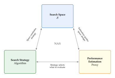
Every NAS method, regardless of its specific algorithmic details, must address three fundamental questions:
Search space : What architectures are possible? The search space defines the set of candidate architectures and thereby determines both the upper bound on achievable performance (no architecture outside can be found, regardless of the search strategy) and the computational cost of the search (a larger space requires more exploration). Search spaces range from small, highly structured spaces (e.g., varying only the width and depth of a fixed architecture template) to large, flexible spaces (e.g., the space of all directed acyclic graphs with arbitrary operations at each node).
Search strategy: How do we explore ? The search strategy is the algorithm that proposes candidate architectures for evaluation. Options include random search, evolutionary algorithms, reinforcement learning, Bayesian optimisation, and gradient-based methods. The choice of strategy determines how efficiently the search converges to good architectures and how robustly it avoids local optima.
Performance estimation: How do we evaluate architectures without full training? Since the inner loop (training an architecture to convergence) is typically the computational bottleneck, practical NAS methods employ approximations: training for fewer epochs, training on a subset of the data, using smaller proxy tasks, or sharing weights across architectures. The accuracy of the performance estimator determines the reliability of the search: a poor estimator may rank architectures incorrectly, leading the search astray.
| Pillar | Method | Key Idea |
| 3*Search Space | Cell-based | Search for a cell (small DAG), then stack cells to form the full network |
| Macro search | Search over the full network topology directly | |
| Hierarchical | Compose cells at multiple levels of granularity | |
| 4*Search Strategy | Random search | Uniformly sample architectures; strong baseline |
| Evolutionary | Maintain a population; mutate, crossover, select | |
| RL-based | Train a controller to generate architectures via policy gradient | |
| Gradient-based | Relax discrete choices to continuous; optimise via backpropagation | |
| 4*[l]Performance | ||
| Estimation | Full training | Train each candidate to convergence; accurate but expensive |
| Weight sharing | Share weights across architectures via a supernet | |
| Early stopping | Train for few epochs; use as proxy for final performance | |
| Predictor-based | Train a surrogate model to predict performance from architecture features |
Remark 5.
The bilevel structure of NAS mirrors the brain's own developmental process at two timescales. The “outer loop” of evolutionary pressure shapes the brain's architecture over generations: species whose genetic programmes produce more effective neural architectures leave more offspring, gradually refining the architectural priors encoded in DNA. The “inner loop” of synaptic plasticity tunes the weights within a single organism's lifetime, optimising the specific wiring configuration for that individual's environment. NAS compresses these two timescales, millions of years of evolution and decades of individual development, into hours or days of computation. The fact that this compression is possible at all reflects the enormous computational power of modern hardware and the ingenuity of the search algorithms we will develop in subsequent sections.
Exercise 5.
Bilevel optimisation for feature selection. Consider a linear regression problem with candidate features and training samples. The true model uses only features. (a) Formulate the feature selection problem as a bilevel optimisation (eq:nas:bilevel,eq:nas:inner-loop) with the search space . (b) Enumerate all architectures and evaluate each by solving the inner loop (ordinary least squares) and computing the validation loss. (c) Verify that the optimal architecture recovers the true feature set. (d) Compare the computational cost of exhaustive search with that of forward stepwise selection. At what value of does exhaustive search become impractical?
Exercise 6.
Weight sharing intuition. Consider a search space of two-layer fully connected networks with hidden width . (a) Explain how a single “supernet” with width can represent all four architectures through masking. (b) Train the supernet on a simple task (e.g., classifying two-dimensional spirals). (c) Evaluate each sub-architecture by applying the appropriate mask to the supernet weights (without retraining) and computing validation accuracy. (d) Compare the supernet-based ranking with the ranking obtained by training each architecture independently from scratch. Do the rankings agree? Discuss potential sources of discrepancy.
Challenge 2.
A brain-inspired NAS algorithm. Design a NAS algorithm that mimics the brain's developmental strategy. Start with a large, randomly connected network. Implement the following: (a) a “synaptogenesis” phase that adds random connections between neurons; (b) a “Hebbian evaluation” phase that strengthens connections whose endpoints are co-activated and weakens others (using the regularised Hebbian rule from (HEBB Continuous)); (c) a “pruning” phase that removes connections whose weights fall below a threshold; (d) a “sleep” phase that globally rescales remaining weights (using (Synaptic Renorm)). Run this algorithm on MNIST or CIFAR-10 and compare the final architecture (after pruning) with architectures found by standard NAS methods. Does the brain-inspired approach find competitive architectures?
Historical Note.
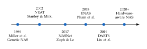
The idea of automatically designing neural network architectures is far older than the term “neural architecture search.” In 1989, David Miller, Philip Todd, and Suresh Hegde used genetic algorithms to evolve the connectivity patterns of small neural networks [8]. In the 1990s and 2000s, the field of neuroevolution flourished, with researchers evolving both architectures and weights using evolutionary algorithms. Kenneth Stanley's NEAT (NeuroEvolution of Augmenting Topologies, 2002) was particularly influential: it evolved neural network topologies by starting with minimal networks and incrementally adding neurons and connections, using a “speciation” mechanism to protect novel architectures from premature extinction by allowing them time to optimise their weights [9]. The modern NAS era began with the work of Zoph and Le (2017), who used reinforcement learning to search for architectures and demonstrated that automatically designed networks could match or exceed the performance of hand-designed ones on image classification benchmarks [10]. The subsequent development of efficient NAS methods (weight sharing, differentiable architecture search, one-shot methods) transformed architecture search from a curiosity requiring thousands of GPU-days into a practical tool that can run on a single GPU in hours.
The Forgetting-Adaptation Tradeoff
We have seen that the brain's architecture evolves throughout life. Neurons sprout new dendrites, synapses strengthen and weaken, and entire cortical regions can be repurposed following injury. But evolution has a price: change something, and you risk breaking something else. A surgeon who rewires the motor cortex to restore movement after a stroke may inadvertently disrupt fine motor control that took decades to refine. The stability-plasticity dilemma haunts both biological and artificial neural systems, and it becomes especially acute when the architecture itself, not merely the weights, is subject to modification.
In previous sections we established the formal framework for describing neural architectures as mathematical objects and showed how search procedures can navigate architecture spaces. Now we confront a deeper question: when the architecture changes to accommodate new capabilities, what happens to the old ones? This question sits at the intersection of neural architecture search and continual learning (26), and its resolution determines whether adaptive networks can be deployed in the real world.
Catastrophic Forgetting Revisited
The phenomenon of catastrophic forgetting, studied extensively in 26, arises when a neural network trained on task is subsequently trained on task and suffers dramatic performance degradation on task . The mechanism is straightforward: the gradient updates that improve performance on task move the parameter vector away from the region of parameter space that was optimal for task . If the loss landscape for task is sharply curved near , even small perturbations can cause large increases in .
The classical analysis of catastrophic forgetting considers a fixed architecture and asks how parameter changes affect performance. But adaptive networks introduce a third dimension to the stability-plasticity dilemma: not just parameter plasticity (how freely should weights change?) but structural plasticity (how freely should the architecture itself change?).
Consider a concrete scenario. A vision transformer has been trained to recognize everyday objects. Now we wish to add medical imaging capabilities. We could simply fine-tune the existing weights, risking catastrophic forgetting of everyday objects. Alternatively, we could add new attention heads specialised for medical features, add new layers for fine-grained texture analysis, or even replace some existing components with more suitable ones. Each structural change carries its own risk of forgetting.
The key insight is that structural changes can be more or less disruptive than parameter changes, depending on how they interact with existing computations. Adding a new module that operates in parallel with existing ones (e.g., a new attention head) is relatively safe. Replacing an existing module (e.g., swapping a convolutional layer for an attention layer) is inherently risky. Removing a module is the most dangerous of all, since it destroys the computations that module performed.
To reason formally about these distinctions, we need a measure of architectural capacity for change.
Definition 9 (Architecture Plasticity).
The architecture plasticity of an architecture is the capacity of to accommodate new tasks without degrading performance on existing ones. Formally, (ARCH Plasticity) where the supremum is taken over all sets of tasks that can be learned sequentially such that, for each prior task and a tolerance , the forgetting is bounded: (Bounded Forgetting) An architecture with can, in principle, learn an unlimited number of tasks without forgetting. In practice, depends on , on the similarity of tasks, and on the total capacity (number of parameters) of .
The definition captures an important asymmetry: a narrow, deep network may have high representational capacity (it can approximate complex functions) but low plasticity (its parameters are tightly coupled, so changing one layer affects all subsequent layers). A wide, modular network may have lower representational capacity per parameter but higher plasticity because modules can be modified independently.
Historical Note.
The stability-plasticity dilemma was first articulated by Stephen Grossberg in the 1980s in the context of adaptive resonance theory (ART) [11]. Grossberg asked a deceptively simple question: how can a learning system incorporate new information without corrupting previously learned knowledge? The question predates modern deep learning by decades, yet it remains one of the most fundamental unsolved problems in artificial intelligence.
In the biological setting, the brain resolves the dilemma through a combination of complementary learning systems (the hippocampus for rapid learning and the neocortex for slow consolidation), structural plasticity (growing new synapses and pruning old ones), and sleep (offline consolidation of new memories into long-term storage). Each of these mechanisms has computational analogues that inform modern approaches to adaptive neural networks, though none has been fully replicated in artificial systems.
The extension of the stability-plasticity dilemma from parameters to architectures is a more recent development, driven by the emergence of neural architecture search and the growing interest in continual learning at scale. The realisation that structural changes to a network can be both more powerful and more dangerous than parametric changes has opened a new frontier in the study of adaptive systems.
How does architecture change affect forgetting? The following proposition quantifies the relationship.
Proposition 8 (Forgetting Under Architecture Change).
Let be an architecture trained to optimality on task 1, achieving parameters . Suppose architecture is obtained by modifying , and let denote the optimal parameters of after training on task 2. Then the forgetting on task 1 is bounded by (Forgetting Bound) where is the Fisher information matrix of the model on task 1, is the Fisher norm, and is an architectural divergence measuring the structural difference between and .
Proof.
We decompose the forgetting into a parameter component and a structural component. Let denote the loss on task 1 for parameters under architecture . We write (Forgetting Decomp) For the parameter shift term, we apply a second-order Taylor expansion of around under architecture . Since is a local minimum, the gradient vanishes, and we obtain (Taylor Param) where is the Hessian of at . For cross-entropy and negative log-likelihood losses, near a local minimum (the Bartlett identity). The parameter shift term is therefore bounded by . Taking the square root and using the concavity of the square root function, this is bounded by when the norm is at most 2.
For the structural shift term, we define the architectural divergence (ARCH Divergence DEF) which captures the maximum loss difference attributable purely to structural change, holding parameters fixed. Combining both terms yields the claimed bound.
Remark 6.
The bound in Proposition 8 reveals two independent sources of forgetting. The first term, , is the classical parameter-level forgetting studied in Elastic Weight Consolidation [6] and related methods. The second term, , is a purely structural contribution that has no analogue in fixed-architecture continual learning. This structural term explains why architecture changes can be more disruptive than simple fine-tuning: even if the parameters remain identical, changing the computational graph through which they operate can alter the function computed by the network.
The bound suggests a practical strategy: when modifying an architecture, minimise both terms simultaneously. The parameter term can be controlled by regularisation (EWC, online EWC, synaptic intelligence). The structural term can be controlled by restricting architecture changes to additions rather than modifications or deletions, since adding a new module with zero-initialised weights yields initially. This observation motivates the “grow, don't replace” principle that we will encounter repeatedly in subsequent sections.
What to Remember, What to Forget
Not all forgetting is catastrophic. In fact, some forgetting is desirable. A model that remembers every detail of its training data is overfitting; a model that retains outdated information about a changed world is making incorrect predictions. The challenge is not to prevent all forgetting but to control what is forgotten and when.
This reframing transforms forgetting from a bug into an optimisation problem: given a set of tasks and a limited budget of model capacity, which knowledge should be retained, which should be discarded, and which should be restructured into a more compact representation? The answer depends on a hierarchy of objectives, ordered from most to least important.
Human preferences (alignment objectives). Certain behaviours must be preserved regardless of efficiency considerations. Safety constraints, ethical boundaries, and user preferences define inviolable requirements. Knowledge that supports these objectives must be protected at all costs.
Task performance (validation metrics). Among the remaining knowledge, priority goes to information that contributes most to performance on current and anticipated future tasks. Performance is measured on validation sets that represent the deployment distribution.
Efficiency (latency, memory, energy). Knowledge that can be preserved with fewer parameters or cheaper computations is preferred. This objective motivates compression and distillation as forms of “productive forgetting.”
Simplicity (Occam's razor). All else being equal, simpler representations are preferred. Complexity that does not contribute to performance or safety is a liability, because it increases the attack surface for adversarial inputs and makes the model harder to interpret.
To operationalise this hierarchy, we need a way to measure how important each piece of knowledge is.
Definition 10 (Knowledge Importance Score).
For each parameter (or, more generally, each module ) in a network, the knowledge importance score is (Importance Score) where is the set of tasks, is a weight reflecting the importance of task in the hierarchy above, and is the loss on task . The score measures how sensitive the aggregate performance is to changes in : parameters with high are critical for multiple important tasks and should be protected; parameters with low can be safely modified or pruned.
The importance score connects directly to the Fisher information matrix. Recall that the diagonal of the empirical Fisher for task has entries . Thus the importance score is a weighted sum of Fisher diagonals: (Importance Fisher)
This reveals a deep connection between selective forgetting and Elastic Weight Consolidation (EWC) [6], which was developed in the continual learning literature (26). EWC adds a quadratic penalty to the loss for task , where is the Fisher diagonal from task and is the optimal parameter for task . Through the NAS lens, EWC is protecting the architecture: it ensures that the parameters most important for task 's computations remain close to their optimal values, thereby preserving the functional structure of the network even as new task knowledge is incorporated.
The connection to bilevel optimisation is immediate. In a bilevel NAS framework, the outer objective decides which knowledge to protect by setting the task weights . The inner objective then optimises the parameters subject to these protection constraints. The outer objective can be viewed as a meta-learner that allocates the network's limited capacity across tasks, deciding which tasks deserve dedicated architectural resources and which can share.
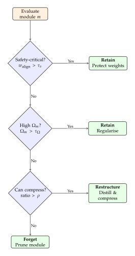
Figure 6 illustrates the decision process for each module. The tree encodes the priority hierarchy: a module that is safety-critical is retained regardless of its efficiency, while a module that is neither safety-critical nor important for any task can be safely pruned. Between these extremes lies the interesting territory of restructuring: modules that contain useful knowledge but in an inefficient form can be distilled into smaller, faster components.
The decision tree is not merely a heuristic; it can be formalised as a constrained optimisation problem. Let indicate whether module is retained () or pruned (), and let indicate the compression ratio applied to retained modules. The selective forgetting problem is then (Selective Forgetting OPT) where is the computational cost of module at compression ratio , and is the set of safety-critical modules. The first term penalises forgetting important knowledge; the second penalises computational cost. The constraint ensures that safety-critical modules are never pruned.
Bilevel Optimisation: Who Decides the Architecture?
The selective forgetting framework raises a meta-question: who decides the task weights , the thresholds and , and the trade-off parameter ? In classical machine learning, these are hyperparameters tuned by the practitioner. But in an adaptive system, they should themselves be learned. This leads naturally to a bilevel optimisation structure.
The bilevel formulation of NAS separates concerns into two nested loops. The inner loop optimises the network's weights for a given architecture , minimising the training loss: (Inner LOOP) The outer loop optimises the architecture (and possibly the meta-parameters , , etc.) to minimise a validation loss: (Outer LOOP) Together, these form the bilevel optimisation problem (Bilevel)
This structure is both natural and problematic. It is natural because it separates the “what to compute” question (architecture) from the “how to compute it” question (weights). It is problematic because the inner optimisation is itself an expensive procedure: fully training a network for each candidate architecture is computationally prohibitive.
The breakthrough insight of DARTS (Differentiable Architecture Search) [25] was to approximate the inner optimisation with a single gradient step, turning the bilevel problem into a tractable alternating optimisation. At each iteration, DARTS performs one gradient step on using and one gradient step on the architecture parameters using . The convergence properties of this procedure are characterised by the following theorem.
Theorem 3 (Bilevel NAS Convergence).
Suppose the inner problem is -strongly convex in for each , and the outer objective is -Lipschitz continuous in . Then the bilevel NAS procedure with inner learning rate and outer learning rate , after outer iterations each with inner steps, satisfies (Bilevel Convergence) The first term is the outer optimisation error, which decreases with the number of outer iterations. The second term is the inner approximation error, arising from the fact that we solve the inner problem only approximately.
Proof.
The proof proceeds in two stages. First, we bound the error introduced by the approximate inner solution. Second, we apply standard results from online convex optimisation to the outer loop.
Stage 1: Inner approximation error. After steps of gradient descent with learning rate on the -strongly convex inner problem, the parameter iterate satisfies (see, e.g., [12]) (Inner Error) Let denote the inner approximation gap. By the Lipschitz continuity of with respect to (with constant ), we have (VAL Inner Error) For a single inner step (), the error is , giving an inner approximation error of .
Stage 2: Outer optimisation. We treat the outer loop as an instance of online gradient descent on the function . Under the Lipschitz assumption, the standard regret bound for online gradient descent with learning rate gives (Outer Regret) Combining the inner approximation error with the outer regret bound, and noting that , we obtain the claimed bound .
The theorem reveals a fundamental tension in bilevel NAS: reducing the inner approximation error requires either more inner steps (increasing cost) or a smaller inner learning rate (slowing convergence). The outer optimisation error decreases with , but each outer step requires at least one inner step. The total cost is therefore gradient evaluations. For the DARTS approximation (), the cost is but the inner approximation error is , which does not vanish. This non-vanishing bias is one of the known failure modes of DARTS and motivates more sophisticated bilevel solvers.
When multiple objectives conflict, the bilevel framework naturally accommodates multi-objective optimisation through Pareto optimality.
Remark 7.
Consider two architectures: achieves 95% accuracy with 100ms latency, while achieves 90% accuracy with 50ms latency. Neither dominates the other: is better on accuracy, is better on latency. Both lie on the Pareto frontier, the set of all architectures for which no single objective can be improved without degrading another. The outer loop of bilevel NAS can be configured to search for architectures on this frontier by scalarising the objectives: , where traces the frontier as it varies. Alternatively, evolutionary methods can maintain a population of non-dominated solutions.
The bilevel framework also connects to reinforcement learning from human feedback (RLHF), as developed in 25. In RLHF, a reward model scores model outputs based on human preferences. This reward model can serve as the outer objective in a bilevel NAS framework: the inner loop trains the model to generate outputs, and the outer loop modifies the architecture to maximise the reward model's score. In this view, RLHF reward models provide architecture-level feedback, not just weight-level feedback. The distinction is subtle but important: a reward model that consistently penalises certain types of errors may indicate that the architecture lacks the representational capacity to avoid those errors, suggesting that structural changes (not just weight updates) are needed.
Are Current LLMs Good Enough?
The preceding analysis raises a provocative question about the dominant paradigm in modern AI. Current large language models (LLMs) are deployed with fixed architectures: the number of layers, the number of attention heads, the hidden dimension, the vocabulary size, and the positional encoding scheme are all determined before training begins and remain immutable throughout training and deployment. Is this a limitation?
The evidence suggests that it is. Consider the phenomenon of attention decay in long conversations. As a conversation grows, the context window fills, and information from earlier turns receives progressively less attention. This is not merely a computational issue (longer contexts require more compute); it is an architectural issue. The attention mechanism allocates a fixed number of heads with fixed key-query dimensions across all parts of the input, regardless of the complexity or importance of each segment.
Insight.
Current LLMs have a fixed architecture. They cannot grow new attention heads for new domains, add memory modules for unfamiliar tasks, or prune irrelevant pathways during inference. The brain, by contrast, adapts its architecture continuously: neurons that fire together wire together, unused synapses are pruned, and new dendritic spines form in response to novel stimuli. Is the fixed architecture of LLMs a fundamental limitation, or can adaptive attention and dynamic computation solve these problems within the existing paradigm? The answer may determine the trajectory of AI for the next decade.
Several concrete failure modes illustrate the limitations of fixed architectures. First, uniform compute allocation: a fixed transformer spends the same number of floating-point operations on the sentence “The cat sat on the mat” as on a complex mathematical proof, despite the vastly different computational requirements. Mixture-of-experts (MoE) models partially address this by routing tokens to specialised experts, but the set of experts is still fixed at training time.
Second, fixed context windows: the positional encoding scheme and attention pattern are determined at training time and cannot adapt to inputs that require longer-range dependencies. Techniques like RoPE extrapolation and sliding-window attention mitigate this, but they are engineering workarounds rather than architectural solutions.
Third, frozen specialisation: a model trained primarily on English text cannot dynamically allocate more capacity to Mandarin when deployed in a Mandarin-speaking region. Fine-tuning helps, but it modifies the entire model rather than adding targeted capacity, risking catastrophic forgetting of English capabilities.
To make the comparison concrete, Table 4 contrasts the two paradigms across several dimensions.
| Property | Fixed Architecture | Adaptive Architecture |
| Capacity allocation | Fixed at design time; same compute for easy and hard inputs | Dynamic; allocate more compute to harder inputs, less to easy ones |
| [4pt] Domain expertise | Shared across all domains; no specialisation possible after training | Specialised modules can be grown for new domains; experts activated on demand |
| [4pt] Memory usage | Constant regardless of task; entire model loaded even for simple queries | Variable; load only relevant modules, offload unused ones |
| [4pt] Deployment complexity | Simple: one model binary, one inference engine | Complex: model surgery, dynamic loading, compatibility management |
| [4pt] Theoretical guarantees | Well-understood: PAC bounds, generalisation theory, scaling laws | Nascent: few convergence guarantees, limited scaling theory |
| [4pt] Continual learning | Requires full retraining or careful fine-tuning with forgetting mitigation | Natural: grow new modules for new tasks, protect existing ones |
The table reveals that the choice between fixed and adaptive architectures is not a simple one. Fixed architectures dominate current practice for good reasons: they are simple to deploy, well-understood theoretically, and benefit from years of engineering optimisation. But as models grow larger and are expected to handle increasingly diverse tasks, the limitations of fixed architectures become more apparent.
The forgetting-adaptation tradeoff is central to this comparison. A fixed architecture has no structural plasticity ( in the sense of Definition 9), meaning that all adaptation must occur in parameter space. An adaptive architecture can, in principle, achieve by growing new modules for new tasks, but this comes at the cost of increased complexity in both training and deployment.
The question is not whether adaptive architectures are theoretically superior (they are, by construction, since they contain fixed architectures as a special case) but whether the practical challenges of adaptive architectures can be overcome.
To sharpen this point, consider the computational cost of adaptation. A fixed architecture can be deployed as a single optimised binary with well-understood latency characteristics. An adaptive architecture requires infrastructure for model surgery (adding, removing, or modifying modules at runtime), dynamic loading (bringing specialised modules into memory on demand), and compatibility management (ensuring that new modules work correctly with existing ones). These engineering challenges are substantial but not insurmountable: modern serving frameworks already support dynamic batching, model parallelism, and mixture-of-experts routing, all of which can be viewed as lightweight forms of architectural adaptation.
Proposition 9 (Capacity-Plasticity Tradeoff).
For a modular architecture with modules, each with parameters, the architecture plasticity (Definition 9) satisfies (Capacity Plasticity) where is the mutual information between module 's parameters and the data of task , and is the forgetting tolerance. The bound shows that plasticity grows linearly with the number of modules (more modules means more capacity for new tasks) and logarithmically with the tolerance (stricter tolerance demands more capacity per task).
Proof sketch.
Each module can accommodate at most tasks before its parameters are fully utilised, by a rate-distortion argument: the parameters encode at most bits of information about task data when the forgetting tolerance is , and each task requires at least bits. Summing over independent modules yields the bound.
The proposition formalises the intuition that modular architectures are more plastic than monolithic ones: by increasing (adding more modules), we can linearly increase the number of tasks the architecture can accommodate. This is the formal justification for the “grow, don't replace” strategy mentioned after Proposition 8.
The remainder of this chapter develops the mathematical and algorithmic tools needed to realise adaptive architectures in practice.
The Landscape of Search Spaces
Before we can search, we must define what we are searching through. Every detective needs a map of the territory: the streets, the buildings, the dead ends, and the shortcuts. In neural architecture search, the territory is the search space, the set of all candidate architectures that the search procedure is permitted to consider. The design of this search space is arguably the most consequential decision in any NAS pipeline, because it determines both the quality of the best discoverable architecture and the tractability of finding it.
A search space that is too small may exclude the optimal architecture entirely. A search space that is too large may be intractable to explore, even with sophisticated search algorithms. The art of NAS lies in designing search spaces that are large enough to contain excellent architectures but structured enough to be navigable.
What Can Be Searched?
We begin with a formal definition.
Definition 11 (Search Space).
A search space for neural architecture search is a set of candidate architectures, defined by a tuple where:
is the set of allowable operations: the computational primitives from which architectures are built. Common operations include convolutions of various kernel sizes (, , ), dilated convolutions, depthwise separable convolutions, self-attention layers, pooling operations (max, average), skip (identity) connections, normalisation layers (batch norm, layer norm, group norm), and the zero operation (no connection).
is the set of allowable connectivity patterns: the ways in which operations can be composed. This includes directed acyclic graphs (DAGs) of bounded size, chain (sequential) architectures, residual connections, and dense connections.
is the set of macro-structural constraints: global properties that all candidate architectures must satisfy. These include bounds on depth (number of layers), bounds on width (channels per layer), total parameter budget, total FLOP budget, and memory constraints.
An architecture is a specific instantiation: a choice of operation for each edge and a connectivity pattern from satisfying all constraints in .
The definition is deliberately general. In practice, search spaces are structured in specific ways that reflect assumptions about what good architectures look like. Three major paradigms have emerged in the NAS literature.
Cell-based search spaces.
Pioneered by NASNet [51], cell-based search spaces decompose the network into small repeatable units called cells. Each cell is a small directed acyclic graph with a fixed number of input nodes, intermediate nodes, and output nodes. The search procedure determines the operations on each edge and the connectivity pattern within each cell. The complete network is then built by stacking copies of the discovered cell in a predetermined pattern.
Cell-based spaces have a crucial advantage: the search is conducted on a small object (the cell), but the resulting architecture can be scaled to arbitrary depth by stacking more cells. This separation of micro-architecture (cell design) from macro-architecture (stacking pattern) dramatically reduces the search cost. The disadvantage is that it imposes homogeneity: every cell in the network has the same structure, which may not be optimal. Different layers of a network may benefit from different operations, but a cell-based space cannot express this heterogeneity.
Typically, two types of cells are searched: normal cells that preserve spatial dimensions and reduction cells that reduce spatial dimensions (typically by a factor of 2). The macro-architecture specifies where normal and reduction cells are placed.
Layer-based search spaces.
Layer-based search spaces allow heterogeneous layers: each layer can have a different operation, different width, and different connectivity. This is more expressive than cell-based spaces but also more expensive, since the number of decisions scales with the depth of the network rather than the (fixed) size of a cell.
MnasNet [33] and EfficientNet [35] use layer-based search, searching over the type, kernel size, and expansion ratio of each layer independently. The increased expressiveness allows these methods to discover architectures with heterogeneous structure, for instance networks that use larger kernels in early layers (for capturing coarse features) and smaller kernels in later layers (for fine-grained features).
Hierarchical search spaces.
Hierarchical search spaces [74] introduce multiple levels of structure. At the lowest level, primitive operations are composed into motifs. At the next level, motifs are composed into cells. At the highest level, cells are composed into the complete network. Each level is searched separately, and the results are composed to build the final architecture.
Hierarchical spaces offer a middle ground between cell-based and layer-based approaches. They allow heterogeneity at the motif level while maintaining structural regularity at the cell and network levels. The main challenge is defining the interfaces between levels: how motifs connect to form cells, and how cells connect to form networks.
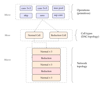
Figure 7 illustrates the three-level hierarchy. The micro level defines the vocabulary of operations; the meso level defines the grammar of cells; the macro level defines the syntax of complete networks. This linguistic analogy is instructive: just as a language's expressiveness depends on both its vocabulary and its grammar, the expressiveness of a search space depends on both the available operations and the ways they can be composed.
| Type | Expressiveness | Search Cost | Notable Methods | |
| Cell-based | – | Medium | 0.5–4 GPU-days | NASNet, DARTS, ENAS |
| [3pt] Layer-based | – | High | 2–20 GPU-days | MnasNet, EfficientNet, OFA |
| [3pt] Hierarchical | – | High | 1–10 GPU-days | Hierarchical NAS, Auto-DeepLab |
| [3pt] Unconstrained | Maximal | 100 GPU-days | NAS-RL (original), random wiring |
Table 5 summarises the key properties of each search space type. The trend is clear: more expressive search spaces are more expensive to search. The cell-based paradigm achieves a favourable trade-off by restricting the search to small, repeatable units, while unconstrained search over arbitrary graph structures remains prohibitively expensive for all but the most well-resourced research groups.
Remark 8.
The choice of search space encodes strong inductive biases. A cell-based space assumes that the optimal architecture is composed of repeated homogeneous units. A layer-based space assumes that layers can be characterised by a small number of discrete choices (operation type, kernel size, expansion ratio). These assumptions are not neutral: they reflect the designer's prior beliefs about what good architectures look like, and they can systematically exclude architectures that violate those beliefs. This is the bias-variance tradeoff of architecture design: a constrained search space has low variance (search is reliable) but potentially high bias (the optimal architecture may be excluded).
The Search Space for Generative Models
The search spaces described above were developed primarily for discriminative tasks, especially image classification. Generative models introduce additional considerations that fundamentally alter which operations and connectivity patterns are relevant.
The search space for a generative model depends on the generative paradigm.
Diffusion models.
The dominant architecture for diffusion models is the U-Net [75], a symmetric encoder-decoder with skip connections at each resolution level. The NAS search space for diffusion models must include: the number and type of residual blocks at each resolution level, the placement and configuration of self-attention layers (which resolutions receive attention, how many heads, what key/query dimensions), the type of normalisation (group norm, layer norm, adaptive group norm), the mechanism for conditioning on the diffusion timestep (additive, multiplicative, adaptive normalisation), and the design of skip connections (simple concatenation, learned gating, attention-based fusion).
The U-Net structure itself imposes a strong prior: the encoder-decoder symmetry and the multi-resolution skip connections are taken as given, and only the internal block designs are searched. Breaking this prior, for instance by searching over asymmetric encoder-decoder architectures, dramatically expands the search space but may discover architectures that outperform the standard U-Net.
Large language models.
The transformer architecture [76] offers a different set of searchable dimensions: the number of attention heads and their dimensions (few large heads vs. many small heads), the ratio of feed-forward network (FFN) hidden dimension to model dimension, the total depth (number of transformer blocks), the attention pattern (full quadratic attention, sparse attention with fixed patterns, linear attention approximations), the positional encoding scheme (absolute, relative, rotary, ALiBi), and the normalisation placement (pre-norm vs. post-norm vs. sandwich norm).
For LLMs, the search space is further complicated by the need to maintain language modelling coherence throughout the architecture. Unlike image classification, where each layer transforms spatial features independently, language modelling requires that information flows coherently from early context to late predictions. An architecture that is optimal for short sequences may perform poorly on long sequences, and vice versa.
Generative adversarial networks.
GANs require searching two architectures simultaneously: the generator and the discriminator. The generator's search space includes the type and arrangement of upsampling blocks (transposed convolution, bilinear upsampling followed by convolution, nearest-neighbour upsampling, sub-pixel convolution), normalisation schemes (batch norm, spectral norm, instance norm, adaptive instance norm), and non-linearities. The discriminator's search space mirrors the generator's but with downsampling blocks and classification-oriented design.
The adversarial training dynamic introduces a unique constraint: the generator and discriminator architectures must be balanced. A generator that is too powerful relative to the discriminator leads to mode collapse; a discriminator that is too powerful leads to vanishing gradients for the generator. This balance constraint couples the two search spaces in ways that have no analogue in discriminative NAS.
To formalise the structure common to all generative NAS search spaces, we introduce the following definition.
Definition 12 (Generative Architecture DAG).
A generative architecture is a directed acyclic graph where:
is a partitioned set of nodes. Input nodes receive data (noise vectors, text tokens, conditioning signals). Intermediate nodes represent internal tensor states. Output nodes produce generated samples (images, audio, text tokens).
is a set of directed edges representing data flow, with the constraint that no directed cycle exists (the graph is acyclic).
assigns an operation from the operation set to each edge. The operation transforms the tensor at the source node to produce (part of) the tensor at the destination node.
For nodes with multiple incoming edges, the incoming tensors are aggregated by a fixed aggregation function (typically element-wise addition or channel-wise concatenation).
The generative architecture DAG provides a common language for describing architectures across different generative paradigms. A U-Net for diffusion is a specific instantiation with a particular connectivity pattern (encoder-decoder with skip connections) and specific operations (residual blocks, attention layers). A transformer for language modelling is a chain DAG with self-attention and FFN operations on each edge. A GAN generator is a DAG with upsampling operations.
Remark 9.
The search space must be rich enough to contain good architectures but constrained enough to be searchable. Too rich and the search is intractable: the number of candidate architectures grows exponentially with the number of nodes and operations, and even sophisticated search algorithms cannot explore more than a tiny fraction of the space. Too constrained and the optimal architecture may lie outside the space entirely. This is the bias-variance tradeoff of architecture design itself: a constrained space has low search variance (the search reliably finds a good architecture within the space) but potentially high bias (the space may not contain the globally optimal architecture).
The design of effective search spaces for generative models remains an active area of research. Unlike discriminative tasks, where decades of manual architecture design have revealed strong structural priors (residual connections, batch normalisation, bottleneck blocks), the generative modelling landscape is younger and less well explored. This means that NAS for generative models has more to discover but also less prior knowledge to guide the search.
To illustrate the differences between generative and discriminative search spaces, consider the following proposition.
Proposition 10 (Generative Search Space Lower Bound).
Let be a cell-based search space designed for discriminative image classification with operations and nodes. A search space for a conditional generative model (e.g., a class-conditional diffusion model) that includes all architectures in plus conditioning pathways must satisfy (GEN Search Lower) where is the number of conditioning mechanisms per node (e.g., additive conditioning, multiplicative conditioning, adaptive normalisation, cross-attention). The multiplicative factor arises because each intermediate node independently chooses how to incorporate conditioning information.
Proof.
Each of the intermediate nodes must process both the input tensor and the conditioning signal. The choice of conditioning mechanism at each node is independent of the operation choices on the edges, giving additional choices per node. By the independence of these choices across nodes, the total number of architectures is at least .
This proposition explains why NAS for generative models is inherently harder than NAS for discriminative models: the search space is exponentially larger due to the additional dimension of conditioning mechanism design. It also highlights the importance of carefully constraining the conditioning search space to maintain tractability.
The Mathematical Structure of Architecture Spaces
Architecture spaces are combinatorial objects with rich mathematical structure. Understanding this structure reveals why some search methods work brilliantly and others fail spectacularly. It explains why gradient-based methods can be applied to inherently discrete objects, why weight sharing enables practical NAS, and where the fundamental limits of efficient architecture search lie.
In this section, we develop the mathematical foundations that underpin modern NAS algorithms. We begin with the combinatorial structure of architecture spaces, proceed to continuous relaxations that enable gradient-based search, and conclude with the supernet paradigm that makes one-shot architecture evaluation possible.
Architecture Spaces as Combinatorial Objects
The first question about any search space is: how large is it? The answer, as we shall see, is typically astronomically large, making exhaustive search impossible and motivating the sophisticated algorithms developed in subsequent sections.
Consider a cell-based search space of the type used in DARTS [25]. A cell is a directed acyclic graph with intermediate nodes, plus two input nodes (representing the outputs of the two preceding cells) and one output node (the concatenation of all intermediate nodes). Each intermediate node receives input from all preceding nodes (both input nodes and intermediate nodes ) via separate edges. Each edge carries one of candidate operations.
Proposition 11 (Search Space Cardinality).
For a cell-based search space with intermediate nodes and candidate operations per edge, where intermediate node (, numbering from the first input node as node 0 and the second input node as node 1) receives input from all preceding nodes , the total number of distinct architectures is (Search Space CARD)
Proof.
Intermediate node (for in our numbering) has exactly incoming edges, one from each of nodes . Each edge independently takes one of operations, giving choices for node . Since the choices for different nodes are independent, the total count is The exponent is .
To appreciate the scale, consider the standard DARTS search space with intermediate nodes and candidate operations (33 separable convolution, 55 separable convolution, 33 dilated convolution, 55 dilated convolution, 33 max pooling, 33 average pooling, and skip connection). The exponent is , giving This is roughly the number of atoms in a human body. Evaluating each architecture for even one second would require more time than the age of the universe. Exhaustive search is out of the question.
But the raw cardinality overstates the true difficulty of the problem, because many distinct DAGs encode the same function. If two edges both carry the zero operation (no computation), swapping them changes the DAG but not the function. More generally, the symmetries of the cell graph create equivalence classes of architectures that compute identical functions.
Proposition 12 (Redundancy Bound).
The number of functionally distinct architectures is at most (Redundancy Bound) where is the automorphism group of the cell graph , consisting of all permutations of intermediate nodes that preserve the edge structure and the identity of input/output nodes.
Proof.
Two architectures and are functionally equivalent if there exists a graph automorphism such that the operation assigned to each edge in equals the operation assigned to the corresponding edge under in . The orbits of under the action of partition the search space into equivalence classes. By the orbit-stabiliser theorem, the number of orbits is at most .
Remark 10.
In practice, the redundancy is even greater than the automorphism bound suggests, because operations themselves can introduce additional symmetries. For instance, if includes both “33 conv followed by ReLU” and “33 conv followed by identity” as separate operations, two architectures differing only in this choice may compute nearly identical functions (since ReLU is close to the identity for positive inputs). Continuous relaxations, discussed next, provide a different and complementary approach to handling this redundancy.
The combinatorial explosion of architecture spaces motivates the central algorithmic challenge of NAS: how to identify good architectures without evaluating more than a tiny fraction of the search space. To put the scale in perspective: if each architecture evaluation took one millisecond, exhaustively evaluating a DARTS search space ( candidates) would require approximately years, which is roughly 900 million times the current age of the universe. Even sampling a mere fraction of the space would take longer than a human lifetime.
The impossibility of exhaustive search means that NAS algorithms must rely on structural properties of the search space to guide their exploration. Two key properties enable efficient search: the smoothness of the loss landscape (nearby architectures tend to have similar performance) and the low intrinsic dimensionality of the set of high-performing architectures (good architectures cluster in a small region of the space). Both properties are empirical observations rather than theoretical guarantees, but they hold consistently across many search spaces and tasks.
The next two subsections develop two key ideas that address this challenge: continuous relaxations (which enable gradient-based search) and supernets (which enable amortised evaluation).
Continuous Relaxations
The architecture search spaces defined above are fundamentally discrete: an architecture is a specific assignment of operations to edges, and the set of such assignments is finite. Discrete optimisation over combinatorial spaces is, in general, NP-hard. The breakthrough that unlocked efficient NAS was the observation that discrete architecture choices can be relaxed into continuous variables, enabling the use of gradient-based optimisation.
The key idea is simple yet powerful: instead of making a hard choice of one operation per edge, allow a soft mixture of all operations and optimise the mixing weights.
Definition 13 (Architecture Parameters).
Let be a search space with edges and candidate operations per edge. The architecture parameters are continuous variables , where represents the strength (or preference) of operation on edge . The discrete architecture is recovered by selecting the dominant operation on each edge: (ARCH Param Discrete)
The continuous relaxation replaces the hard operation selection with a soft weighted combination. For an edge connecting nodes and , the relaxed operation is (Softmax Relaxation) where is the output of operation applied to input . The softmax function ensures that the weights are positive and sum to one, so the relaxed operation is a convex combination of all candidate operations.
When the architecture parameters are “peaked” (one is much larger than the others), the softmax concentrates nearly all weight on a single operation, and the relaxed operation closely approximates the discrete selection. When is “flat” (all are similar), the relaxed operation is a uniform mixture, and the behaviour is far from any single discrete architecture.
This observation leads to a natural question: how well does the continuous relaxation approximate the discrete problem?
Proposition 13 (Relaxation Gap).
Let denote the discrete architecture obtained by selecting on each edge, and let denote the continuous relaxation with softmax weights. Then the loss difference is bounded by (Relaxation GAP) where is a constant depending on the Lipschitz continuity of the loss with respect to operation outputs, and with is the entropy of the architecture distribution. When is peaked (low entropy), the relaxation is tight; when is uniform (high entropy), the gap can be large.
Proof.
We bound the difference edge by edge. For edge , let be the softmax weight of operation , and let . The relaxed output is , while the discrete output is . Their difference is (EDGE DIFF) since the term vanishes. Taking norms and using the triangle inequality, where bounds the maximum operation difference. The quantity measures how far the distribution is from a point mass. By Pinsker-type inequalities, when , and more generally for operations.
If the loss is -Lipschitz with respect to each edge's output, the total loss difference across all edges is bounded by , where and we identify .
The proposition has a clear practical implication: to ensure that the discrete architecture selected from the continuous relaxation performs similarly to the relaxed model, the architecture parameters should be driven toward peaked distributions (low entropy) during training. DARTS achieves this indirectly through optimisation dynamics: as training progresses, the architecture parameters tend to diverge, with one operation per edge accumulating most of the weight. However, this tendency is not guaranteed, and DARTS can suffer from “collapse”: the architecture parameters may concentrate on degenerate operations (especially skip connections) rather than genuinely useful ones.
Key Idea.
The continuous relaxation bridges the gap between the combinatorial world of architecture design and the continuous world of gradient-based optimisation. By replacing hard operation choices with soft mixtures, it transforms the NAS problem from a discrete search over candidates into a continuous optimisation over real-valued parameters. The quality of this bridge depends on the entropy of the architecture distribution: low entropy means a tight bridge; high entropy means the continuous and discrete worlds may disagree.
A more principled approach to the continuous-discrete bridge uses the Gumbel-Softmax reparameterisation trick, which enables discrete sampling while maintaining differentiability.
The idea is to add Gumbel noise to the architecture parameters before applying softmax, yielding a sample from a categorical distribution in the forward pass while allowing gradient computation in the backward pass. Specifically, for each edge and each operation , we sample independently and compute (Gumbel Softmax) where with is a sample from the standard Gumbel distribution, and is a temperature parameter.
The temperature controls the sharpness of the resulting distribution. As , the Gumbel-Softmax distribution approaches a one-hot categorical distribution: one approaches 1 and the rest approach 0. As , the distribution approaches uniform: all approach .
Proposition 14 (Gumbel-Softmax Properties).
The Gumbel-Softmax distribution has the following properties:
Correct marginals. as the number of samples grows, regardless of .
Discrete limit. As , where and is the -th standard basis vector. The sample becomes exactly one-hot.
Differentiability. For any , the mapping is differentiable almost everywhere, enabling gradient computation via backpropagation through the sampling process.
Variance. The variance of each decreases as , concentrating the distribution and reducing gradient variance. However, very small leads to near-zero gradients (the “straight-through” regime), creating a bias-variance tradeoff in the choice of temperature.
Proof.
Property (1) follows from the Gumbel-Max trick: if with , then . The Gumbel-Softmax is a continuous relaxation of this argmax, and its expectation converges to the same categorical probabilities.
Property (2) follows from the observation that as , for all (since for almost surely), so and all other .
Property (3) is immediate from the composition of smooth functions (exponential, division) applied to the parameters . The Gumbel noise does not depend on , so the gradient exists and is computable.
Property (4) follows from the concentration of the softmax function as : the distribution places nearly all mass on a single operation, so approaches that of a Bernoulli random variable with extreme probability, which is near zero.
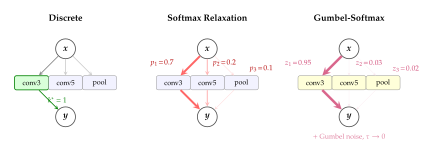
In practice, NAS algorithms using Gumbel-Softmax employ a temperature annealing schedule: training begins with a high temperature (encouraging exploration by keeping the distribution diffuse) and gradually decreases (encouraging exploitation by sharpening the distribution). This schedule mirrors the exploration-exploitation tradeoff in reinforcement learning and connects NAS to the broader family of simulated annealing algorithms.
Figure 8 contrasts the three approaches to operation selection on a single edge. The discrete approach is computationally cheap (only one operation is evaluated) but non-differentiable. The softmax relaxation is differentiable but requires evaluating all operations and produces a blended output that may not correspond to any single discrete architecture. The Gumbel-Softmax strikes a middle ground: it produces near-discrete samples while maintaining differentiability, at the cost of introducing stochasticity into the gradient estimates.
Proposition 15 (Temperature Annealing Convergence).
Consider a Gumbel-Softmax NAS procedure with temperature schedule for outer iteration , where and . As , , and the architecture distribution converges to a point mass on the discrete architecture . Furthermore, if the loss landscape has a unique global minimum and the annealing rate is sufficiently slow (), the procedure converges to in probability.
Proof sketch.
The convergence of ensures that the Gumbel-Softmax distribution concentrates on the argmax of . By Property (1) of Proposition 14, this argmax samples from the categorical distribution . If the gradient-based updates on converge to a fixed point such that places all mass on , then the procedure converges. The condition on ensures that the temperature decreases slowly enough for the gradient updates to track the changing landscape, analogous to the logarithmic cooling schedule in classical simulated annealing (see [13]).
Supernets and Weight Sharing
Continuous relaxations solve the problem of searching over discrete architectures, but they do not solve the problem of evaluating each candidate. Even with gradient-based architecture optimisation, each iteration requires a forward and backward pass through the full relaxed model, which contains all operations on every edge. The computational cost of a single relaxed forward pass is therefore times the cost of evaluating a single architecture.
A more fundamental efficiency concern is that NAS requires evaluating many architectures during the search process. If each evaluation requires full training (hundreds of epochs on a large dataset), the total cost is prohibitive. The supernet paradigm addresses this by training a single shared model from which all candidate architectures can be extracted and evaluated without retraining.
Definition 14 (Supernet (One-Shot Model)).
A supernet (also called a one-shot model) is a single over-parameterised network that contains all candidate architectures as subnetworks. For any architecture , the subnetwork is obtained by selecting the relevant subset of weights corresponding to the operations and connections specified by .
The supernet is trained once, and the performance of any architecture is estimated by evaluating its subnetwork using the shared weights , without any additional training.
The supernet concept is both elegant and radical. Consider a search space with candidate architectures. Training and evaluating each one independently would require training runs. With a supernet, a single training run suffices to obtain weight estimates for all architectures simultaneously. The cost reduction is astronomical: from training runs to one.
The mechanism is weight sharing: all candidate architectures share the same set of weights. If architecture uses a 33 convolution on edge and architecture also uses a 33 convolution on edge (but differs on other edges), they share the same convolutional weights on that edge. This sharing amortises the cost of training across all architectures.
The training procedure for a supernet is straightforward in principle. At each training step: (1) sample an architecture from a distribution over the search space; (2) activate only the operations and connections corresponding to , masking all others; (3) perform a forward pass through the activated subnetwork; (4) compute the loss and backpropagate, updating only the weights used by . Over many training steps, all weights receive gradient updates, but each weight is updated only in the context of architectures that use it.
Caution.
Weight sharing introduces coupling between architectures. The performance of a subnetwork extracted from the supernet may differ significantly from its performance when trained from scratch (its stand-alone performance). This “weight coupling” arises because the shared weights are trained in the context of many different architectures. When operation and operation share upstream weights, training with active affects 's performance, and vice versa. The shared weights must compromise between the conflicting demands of different architectures, leading to suboptimal performance for any single architecture. This coupling is the fundamental challenge of the supernet paradigm and has motivated extensive research into fairer and more accurate weight sharing strategies.
The practical impact of weight coupling is that the ranking of architectures by their supernet performance may differ from the ranking by their stand-alone performance. If the rankings are similar, the supernet is a reliable proxy for architecture evaluation: simply evaluate all (or many) subnetworks in the trained supernet and select the top-ranked one. If the rankings differ significantly, the supernet may lead the search astray, selecting architectures that perform well with shared weights but poorly with dedicated weights.
Definition 15 (Weight Sharing Fidelity).
The fidelity of weight sharing for a set of architectures is defined as the rank correlation between shared and stand-alone performance: (WS Fidelity) where is the validation loss of architecture evaluated using supernet weights, is the validation loss after training from scratch, and converts losses to ordinal ranks. High fidelity () means the supernet ranking is a reliable proxy for true performance; low fidelity () means the supernet provides no useful ranking information.
Empirical studies have found that fidelity varies widely depending on the search space, the supernet training procedure, and the sampling strategy. Early one-shot methods achieved fidelity values of –, barely above random ranking. More recent methods have pushed fidelity above through careful design of the training procedure.
The sampling strategy, which determines how architectures are selected at each training step, is a key factor in fidelity. Different methods make different choices:
Uniform sampling selects each architecture with equal probability. This ensures that all operations receive equal training, but it may not allocate enough training to the most promising architectures.
Path-based sampling (used in ENAS [14]) selects a single path through the supernet DAG at each step, activating exactly one operation per edge. This is memory-efficient (only one operation is computed per edge) but may undertrain operations that are rarely sampled.
Fair sampling (used in FairNAS [15]) ensures that every operation on every edge receives exactly the same number of training steps. This eliminates the bias introduced by non-uniform sampling but requires careful bookkeeping.
Single-path one-shot [16] combines uniform path sampling with a strict training protocol that ensures convergence of all subnetworks. This approach achieves high fidelity by preventing any single architecture from dominating the training.
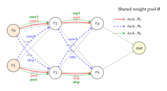
conv3 on edge
, they use identical weights for that operation.
This weight sharing enables evaluating all architectures after a single
training run, at the cost of potential weight coupling.Figure 9 visualises the supernet concept. The complete DAG contains all operations on all edges. Each candidate architecture activates a subset of operations, forming a subnetwork. Different architectures may share operations (and therefore weights) on some edges while differing on others.
| Method | Sampling Strategy | Fidelity () | Search Cost |
| ENAS [14] | RL controller samples paths | 0.5–0.6 | 0.5 GPU-days |
| [3pt] One-Shot [17] | Uniform random dropout of paths | 0.6–0.7 | 1.5 GPU-days |
| [3pt] FairNAS [15] | Strict fair sampling; each operation trained equally | 0.7–0.8 | 2.0 GPU-days |
| [3pt] Single-Path [16] | Uniform single-path; one op per edge per step | 0.75–0.85 | 1.0 GPU-days |
Table 6 compares the major weight sharing strategies along the dimensions of sampling strategy, fidelity, and search cost. The progression from ENAS to Single-Path illustrates the field's evolving understanding of the weight coupling problem: early methods prioritised speed (ENAS completed in half a GPU-day) at the expense of fidelity, while later methods accept modestly higher cost in exchange for more reliable architecture rankings.
The theoretical analysis of weight sharing fidelity remains incomplete. We can, however, state a basic result that connects fidelity to the diversity of the search space.
Theorem 4 (Weight Sharing Error Bound).
Let denote the optimal supernet weights obtained by minimising over the weight pool . For any architecture , let denote the optimal stand-alone weights. Then the performance gap due to weight sharing is bounded by (WS Error Bound) where is the Lipschitz constant of with respect to . Furthermore, the weight difference is bounded by the architectural diversity: (WS Weight DIFF) where is the strong convexity constant of the per-architecture loss. The right-hand side measures the expected gradient magnitude on architecture 's weights when evaluated on a different architecture : the more diverse the search space, the larger this “gradient interference” and the worse the weight sharing approximation.
Proof.
The first inequality follows directly from the Lipschitz assumption on .
For the second inequality , note that the supernet optimality condition requires since minimises the expected loss. The stand-alone optimality condition requires . Taking the difference, (WS GRAD Balance) The first term is the gradient that, if set to zero, would give the stand-alone optimum. Because in general, this gradient is nonzero and equals (in magnitude) the second term: the “interference” from other architectures. By the -strong convexity of , Applying Jensen's inequality to move the norm inside the expectation, and rescaling by , yields the bound .
The theorem provides a formal explanation for an empirical observation: weight sharing works well when the candidate architectures are similar (low gradient interference) and poorly when they are diverse (high gradient interference). This insight has practical implications for search space design: a search space should contain architectures that are diverse enough to include good candidates but similar enough that weight sharing provides reliable rankings.
Key Idea.
The supernet paradigm embodies a fundamental tradeoff: a diverse search space is more likely to contain excellent architectures but makes weight sharing less reliable. A narrow search space yields high-fidelity weight sharing but may exclude the optimal architecture. The art of practical NAS lies in finding the sweet spot where the search space is broad enough to contain good architectures and narrow enough for weight sharing to provide trustworthy rankings.
The supernet paradigm has become the dominant approach in practical NAS, enabling architecture searches that would be computationally infeasible with independent training. Its success rests on two empirical observations: first, that weight sharing fidelity is “good enough” for most search spaces (i.e., the top-ranked architectures by supernet performance tend to be among the top by stand-alone performance, even if the exact rankings differ); and second, that the computational savings are so enormous that even moderate fidelity losses are acceptable.
Looking forward, the supernet paradigm is being extended in several directions. Progressive shrinking [77] trains a single supernet at the largest scale and then “shrinks” it to obtain architectures of different sizes, enabling deployment across devices with different computational budgets. Hardware-aware supernets [32] incorporate latency measurements directly into the training loop, so the supernet learns not just which architectures are accurate but which are fast on target hardware. Multi-task supernets [78] extend weight sharing across tasks, so a single supernet can yield specialised architectures for different tasks.
These extensions represent the frontier of the supernet paradigm, and they share a common theme: leveraging the amortised nature of weight sharing to solve increasingly ambitious architecture search problems. The mathematical foundations developed in this section, including the combinatorial analysis of search spaces, the continuous relaxation framework, and the fidelity analysis of weight sharing, provide the theoretical grounding for these practical advances.
We conclude this section with a concise algorithmic summary of the one-shot NAS procedure built on supernets and continuous relaxations.
Algorithm 1 (One-Shot NAS with Weight Sharing).
Input: Search space , training set , validation set , outer iterations , inner steps , temperature schedule .
Output: Discovered architecture .
Initialise supernet weights and architecture parameters .
For : enumerate
Inner loop (weight training): For : itemize
Sample architecture .
Compute training loss .
Update weights: . itemize
Outer loop (architecture update): itemize
Compute validation loss .
Update architecture parameters: . itemize
Anneal temperature: . enumerate
Discretise: For each edge , select .
Retrain: Train the discrete architecture from scratch to obtain final weights.
Return .
The final retraining step (step 4) is critical. Due to weight coupling (warn:nas:weight-coupling), the supernet weights are suboptimal for any individual architecture. Retraining from scratch with the discovered architecture typically improves performance by 1–3% on standard benchmarks. Some recent methods attempt to skip this step by fine-tuning the supernet weights for the selected architecture, but full retraining remains the gold standard for obtaining final performance numbers.
In the next sections, we turn from the mathematical structure of architecture spaces to the algorithms that navigate them. Armed with continuous relaxations and supernets, we will see how gradient-based methods, evolutionary algorithms, and reinforcement learning agents can discover architectures that match or exceed the best human designs.
Exercise 7.
Consider a neural network trained on task to achieve parameters . The network is then modified by adding a new module with parameters initialised to zero, and trained on task . Show that the initial architectural divergence is zero, and derive a condition on the learning rate that ensures after one gradient step on task .
Exercise 8.
Derive the relationship between the knowledge importance score (Definition 10) and the Fisher information matrix for a single task. Show that when contains a single task , and discuss why the diagonal approximation of is sufficient for computing but may miss interactions between parameters captured by off-diagonal terms.
Exercise 9.
Consider a hierarchical search space with two levels. At the lower level, motifs are built from operations arranged in DAGs with intermediate nodes. At the upper level, cells are built from motifs arranged in DAGs with intermediate nodes, where is the number of distinct motifs. Compute and , and compare their product to the size of a flat search space with and .
Exercise 10.
Implement the Gumbel-Softmax estimator for a search space with operations and a single edge. Compute the variance of the gradient estimator as a function of the temperature . Plot the variance and discuss the bias-variance tradeoff in choosing .
Exercise 11.
Design an experiment to measure the weight sharing fidelity of a supernet. Describe how you would: (a) define the search space, (b) train the supernet, (c) sample a set of architectures and evaluate their supernet performance, (d) train each sampled architecture from scratch and evaluate its stand-alone performance, and (e) compute and report . What is the minimum number of architectures needed to obtain a statistically reliable estimate of ?
Exercise 12.
Consider a NAS problem with two objectives: accuracy and latency . Define the Pareto frontier formally, prove that it is a connected curve in the plane under mild continuity assumptions, and show that any architecture on the frontier can be obtained by solving for an appropriate (assuming convexity of the Pareto frontier).
Reinforcement Learning-Based NAS
The modern neural architecture search story begins with a bold idea: what if we trained a neural network to design other neural networks? In 2017, Barret Zoph and Quoc Le did exactly that, using reinforcement learning to automate architecture design [18]. The result was architectures that matched or exceeded human-designed ones on competitive benchmarks, but at a staggering computational cost: 800 GPUs running for 28 days. This section develops the mathematical framework behind reinforcement learning-based NAS, analyses its strengths and weaknesses, and explains why its sheer computational extravagance motivated the efficient alternatives that followed.
The core idea is elegant in its simplicity. A controller network learns to generate architecture descriptions by trial and error. Each generated architecture is trained and evaluated, and the resulting performance serves as a reward signal that guides the controller toward better designs. The controller is itself a neural network, so we arrive at the recursive spectacle of a neural network learning to design neural networks.
NAS with Reinforcement Learning (Zoph & Le, 2017)
Historical Note.
The paper that launched modern NAS appeared at ICLR 2017 [18]. Zoph and Le used a recurrent neural network (RNN) controller trained with the REINFORCE algorithm [19] to generate architecture descriptions as sequences of tokens. Each token specifies a layer type, kernel size, number of filters, or stride value. The controller generates a complete “child network” specification, which is then trained to convergence on the target task, and the validation accuracy of the trained child becomes the reward signal for the controller. The search required 800 GPU-days of computation (approximately 19,200 GPU-hours) and produced an architecture achieving 3.65% test error on CIFAR-10, competitive with the best human-designed networks of the time. The paper demonstrated that automated architecture design was not merely feasible but could match expert performance, and it ignited an explosion of research that produced over a thousand follow-up papers within three years.
The controller RNN.
The controller is a long short-term memory (LSTM) network [79] that outputs a sequence of actions (tokens) specifying the child architecture. For a convolutional network with layers, the controller produces tokens: for each layer , it outputs the filter height , filter width , number of filters , and stride . The tokens are generated autoregressively: each token is sampled from a softmax distribution conditioned on all previous tokens, and the sampled token is fed back as input to the next time step.
Definition 16 (Controller Policy).
The controller defines a stochastic policy parameterised by LSTM weights , where action specifies layer 's hyperparameters. For a convolutional search space, the action at layer is the tuple consisting of filter height, filter width, number of filters, and stride. The full architecture is the action sequence (Architecture Sequence) and the joint probability of generating under the policy is (Policy PROB)
The reward signal.
Once the controller samples an architecture , a child network with that architecture is constructed and trained from scratch on the training set until convergence (or for a fixed number of epochs). Let denote the trained parameters. The reward is the validation accuracy of the trained child: (Reward) This reward is non-differentiable with respect to the controller parameters because it depends on the discrete architecture and the outcome of an entire training run. Reinforcement learning provides the tools to optimise despite this non-differentiability.
Algorithm 2 (RL-Based Neural Architecture Search).
- Input: Controller policy ; search space ; number of iterations ; controller learning rate ; baseline decay
- Initialise controller parameters randomly
- Initialise baseline
- for
- Sample architecture Controller generates child specification
- Construct child network
- Train child to convergence: Full training run
- Evaluate reward
- Update baseline Exponential moving average
- Compute policy gradient estimate:
- Update controller:
- return best architecture
The algorithm is conceptually straightforward but computationally devastating. Step 6 requires training a full neural network to convergence for every sampled architecture. With on the order of thousands, and each training run requiring hours of GPU time, the total cost is enormous.
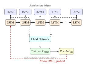
REINFORCE and Policy Gradient for Architecture Search
The controller's objective is to maximise the expected reward over architectures sampled from its policy: (RL Objective) Since is non-differentiable with respect to (it involves discrete sampling and an entire training procedure), we cannot compute by backpropagation through the reward. Instead, we apply the policy gradient theorem, also known as the REINFORCE estimator [19].
Definition 17 (Policy Gradient for NAS).
The policy gradient of the NAS objective (RL Objective) is (Policy Gradient) This identity holds because , which allows the gradient to be written as an expectation under the current policy, enabling Monte Carlo estimation.
Derivation.
Starting from the definition of : (Reinforce Derivation) The second line uses the fact that does not depend on (the reward is a constant for a given architecture). The third line applies the log-derivative trick: .
Variance reduction via baseline.
The raw REINFORCE estimator suffers from high variance because the reward can vary substantially across sampled architectures. A standard technique is to subtract a baseline that does not depend on the current action: (Reinforce Baseline) where is the number of sampled architectures per update and is typically an exponential moving average of past rewards. The baseline does not introduce bias: . The optimal baseline (minimising variance) is the weighted expectation , but the exponential moving average is a practical and effective approximation.
Proposition 16 (Sample Complexity of RL-NAS).
Let be a finite search space and let be the optimal reward. Suppose for all . The number of architecture evaluations needed by any algorithm (including RL-NAS) to find an architecture satisfying with probability at least is (Sample Lower Bound)
Proof.
We reduce to a multi-armed bandit lower bound. Consider each architecture as an arm with expected reward . An algorithm that finds an -optimal arm with probability must distinguish arms whose means differ by at most .
Fix two architectures with . By the Neyman–Pearson lemma, any test distinguishing these two hypotheses from independent observations requires (Neyman Pearson Bound) where captures the noise in reward estimates (due to stochastic training, data sampling, and architectural variation). Applying a union bound over the arms and noting that the hardest pair determines the lower bound, we obtain
Caution.
The original NAS experiment consumed approximately 800 GPU-days, equivalent to roughly 19,200 GPU-hours. At 2017 cloud computing prices, this corresponds to approximately $50,000 in compute costs. For perspective, training a single ResNet-110 on CIFAR-10 takes roughly 0.25 GPU-days. The NAS controller evaluated approximately 12,800 child architectures, each trained for 50 epochs. This computational barrier placed NAS beyond the reach of all but the most well-resourced laboratories and became the primary motivation for the efficient methods developed in sec:nas:enas,sec:nas:darts,sec:nas:modern.
The computational tragedy.
The fundamental inefficiency of RL-based NAS lies in a simple observation: most of the computation goes to training child networks that are immediately discarded. Of the 12,800 architectures evaluated by Zoph and Le, only the single best one was ultimately used. The remaining 12,799 training runs produced parameters that were thrown away after a single validation accuracy measurement. Every child network is trained from scratch, with no knowledge transfer from previously trained children. This is analogous to solving a jigsaw puzzle by independently attempting every possible arrangement from scratch, rather than building incrementally on partial solutions.
Extensions to the search space.
Zoph et al. (2018) extended the approach to search for cells rather than entire architectures [23]. A cell is a small computational graph (typically 5–7 nodes) that is repeated and stacked to form the full network. This cell-based search reduces the search space dramatically while allowing the discovered cell to transfer across datasets: a cell found on CIFAR-10 can be stacked more times to build a competitive ImageNet model. The NASNet architecture, discovered through this cell-based search, achieved 82.7% top-1 accuracy on ImageNet, a state-of-the-art result at the time.
Remark 11.
While the original work used REINFORCE, subsequent RL-based NAS methods explored alternative reinforcement learning algorithms. Proximal Policy Optimisation (PPO) [20] was used for more stable controller training. Baker et al. [21] used Q-learning to explore the architecture space. Real et al. [22] showed that evolutionary methods (tournament selection with mutation) could match or exceed RL-based search, achieving 3.34% error on CIFAR-10 with the base AmoebaNet (and as low as 2.13% when the discovered cell is scaled up), at a search cost of 3,150 GPU-days. The diversity of search strategies suggested that the search algorithm itself was less important than the search space design and the evaluation protocol.
ENAS: Efficient NAS via Parameter Sharing
The single most wasteful aspect of RL-based NAS is that each child network is trained from scratch. Pham et al. (2018) [24] asked a simple but transformative question: what if child networks shared their weights? The answer was ENAS (Efficient Neural Architecture Search), which reduced the search cost from 800 GPU-days to 0.5 GPU-days, a speedup of 1,600 times, by having all candidate architectures share parameters through a single large “supernet.”
The Parameter Sharing Insight
The key observation is that child networks in RL-NAS are not independent: they share similar computations. A convolution at layer 5 performs the same type of computation regardless of what operations surround it. If one child has already trained this convolution, a second child that also uses a convolution at layer 5 should be able to reuse the learned filters rather than learning them from scratch.
Definition 18 (ENAS Supernet).
A supernet (also called a one-shot model) is a single directed acyclic graph that contains all candidate operations on each edge. Formally, for each edge , the supernet maintains a set of operations , each with its own parameters. A candidate architecture is a subgraph of obtained by selecting exactly one operation per edge: (Subgraph) All architectures share the supernet's weight pool . A controller selects which subgraph to activate at each training step.
Key Idea.
ENAS amortises the cost of training across all architectures. Instead of training each child from scratch, every child inherits pre-trained weights from the supernet. The supernet serves as a shared memory: when one architecture trains the convolution at layer 5, all other architectures that use the same operation at the same layer benefit from the updated weights. This transforms the cost from (where is the number of architectures and is the cost of training one child) to (the cost of training the supernet once), a reduction from thousands of GPU-days to a single GPU-day.
Training procedure.
ENAS alternates between two phases in each iteration:
Supernet weight update. Fix the controller parameters . Sample an architecture , activate the corresponding subgraph of the supernet, and update the shared weights using standard stochastic gradient descent on the training loss: (ENAS Weight Update) Only the weights belonging to the active subgraph receive gradient updates.
Controller update. Fix the supernet weights . Sample architectures from . Evaluate each on the validation set (without any further training) and compute rewards . Update the controller with REINFORCE: (ENAS Controller Update)
Algorithm 3 (ENAS Training Loop).
- Input: Supernet with shared weights ; controller ; training set ; validation set ; learning rates ; baseline decay
- Initialise and randomly; set baseline
- for epoch
- for each minibatch
- Phase 1: Train supernet weights
- Sample Controller generates architecture
- Activate subgraph in supernet
- Update only active weights
- for
- Phase 2: Train controller
- Sample
- Evaluate on validation set, no training
- Derive final architecture
- Retrain from scratch on full training set
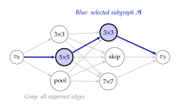
Convergence Analysis
Parameter sharing introduces a fundamental approximation: the supernet weights (the subset of supernet weights used by architecture ) are not the same as the weights that would be obtained by training from scratch. This raises two questions. First, how large is the approximation error? Second, does the supernet preserve the ranking of architectures?
Theorem 5 (ENAS Weight Sharing Approximation).
Let be -Lipschitz continuous in its first argument (the network parameters). For any architecture in the search space, the validation loss evaluated with the supernet weights (restricted to ) satisfies (ENAS Approx Bound) where are the optimal stand-alone weights for .
Proof.
By the definition of Lipschitz continuity, for any two parameter vectors and fixed architecture : Setting (supernet weights restricted to ) and (optimal stand-alone weights) yields the result directly.
The bound in Theorem 5 is tight in the sense that the Lipschitz constant cannot be removed. However, the bound is only useful if is small, which is an empirical question that depends on how well the supernet training distributes capacity across architectures.
The ranking correlation problem.
For NAS, the absolute quality of each architecture's evaluation matters less than the ranking: we need the supernet to correctly identify which architectures are better than which. The standard measure is Kendall's rank correlation between the supernet ranking and the true ranking (obtained by training each architecture from scratch). Empirical studies report moderate correlations of –, indicating that the supernet ranking is informative but imperfect.
Proposition 17 (Ranking Preservation Condition).
Let denote the true validation loss and denote the supernet validation loss. The supernet preserves the ranking of two architectures (i.e., if then ) whenever (Ranking Condition)
Proof.
By the triangle inequality applied to Theorem 5, we have for each architecture: For the ranking to be preserved, we need . A sufficient condition is that the upper bound for is below the lower bound for : Rearranging: This is a stronger condition than stated. A necessary condition for ranking reversal is that the approximation errors are large enough to bridge the gap between the true losses, which yields the stated bound as a sufficient condition for preservation.
The proposition reveals that ranking preservation depends on two factors: the gap between the true losses (large gaps are easier to preserve) and the uniformity of approximation errors (if all architectures have similar approximation error, rankings are preserved even when the absolute error is large).
| Method | Search Cost | CIFAR-10 | Penn Treebank |
| (GPU-days) | Error (%) | PPL | |
| NAS [18] | 800 | 3.65 | 62.4 |
| NASNet [23] | 1,800 | 2.65 | – |
| ENAS [24] | 0.5 | 2.89 | 55.8 |
| Random search baseline | 0.5 | 3.29 | 67.1 |
DARTS: Differentiable Architecture Search
ENAS shared weights but still used REINFORCE to search over architectures. Liu, Simonyan, and Yang (2019) [25] asked whether the architecture search itself could be made differentiable. If so, gradient descent, the most efficient optimisation tool available, could search over architectures directly. The result was DARTS (Differentiable Architecture Search), which replaced discrete architecture choices with a continuous relaxation, enabling end-to-end gradient-based optimisation of both the network weights and the architecture.
Making Architecture Search Differentiable
The central insight of DARTS is to replace discrete choices with continuous mixtures. Rather than selecting a single operation on each edge of the cell DAG, DARTS computes a weighted sum of all candidate operations, where the weights are determined by learnable architecture parameters.
Definition 19 (DARTS Mixed Operation).
For each edge in the cell directed acyclic graph, DARTS computes the mixed operation: (Darts Mixed OP) where is the set of candidate operations and are the architecture parameters. During search, all operations execute in parallel with softmax-weighted mixing. After search, the final architecture retains only the dominant operation on each edge: .
The softmax weighting makes the output differentiable with respect to , which is the key property enabling gradient-based search. As the architecture parameters converge, the softmax distribution concentrates on a single operation, and the continuous relaxation approaches a discrete architecture.
Bilevel optimisation formulation.
DARTS optimises two sets of parameters simultaneously: the network weights (convolution filters, batch normalisation parameters, etc.) and the architecture parameters . The weights are trained on the training set, while the architecture parameters are optimised on the validation set. This is naturally expressed as a bilevel optimisation problem: (Darts Bilevel) The outer problem ((Darts Bilevel)) seeks architecture parameters that minimise the validation loss, while the inner problem ((Darts Bilevel)) requires that the network weights are optimal for the current architecture.
Algorithm 4 (DARTS: Differentiable Architecture Search).
- Input: Cell DAG with edges ; candidate operations ; training set ; validation set ; learning rates ; inner approximation step size
- Initialise network weights randomly
- Initialise architecture parameters uniformly Equal weight on all operations
- while not converged
- Step 1: Update weights (inner optimisation)
- Sample minibatch from
- Step 2: Update architecture (outer optimisation)
- Sample minibatch from
- Compute one-step approximation:
- Approximate hypergradient
- Step 3: Derive discrete architecture
- for each edge
- Select operation
- Retrain derived architecture from scratch Standard training
The search cost of DARTS is approximately 1.5 GPU-days on CIFAR-10, which is cheaper than the original NAS and more expensive than ENAS. However, DARTS achieves 2.76% test error on CIFAR-10, competitive with the best NAS results.
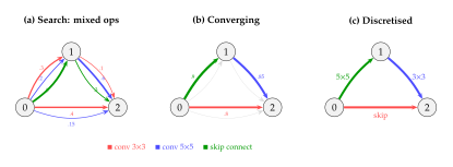
The Bilevel Optimisation Problem
The outer objective in (Darts Bilevel) depends on both directly and through . Computing the full gradient requires implicit differentiation through the inner optimisation, which involves the Hessian of the training loss.
The hypergradient.
By the implicit function theorem, the gradient of the outer objective with respect to is: (Darts Hypergradient) where all quantities are evaluated at and is the inner learning rate. The second term involves the inverse Hessian , which is prohibitively expensive to compute for large networks.
First-order approximation.
The simplest approximation sets , which eliminates the second-order term entirely. The approximate gradient is simply: (Darts First Order) where is the current (not optimal) weight vector. This is cheap to compute (a single backward pass through the validation loss) but ignores the dependence of on .
Second-order approximation.
DARTS approximates the Hessian-vector product using finite differences. Let and choose a small . Then: (Darts Finite DIFF) This requires two additional forward-backward passes (at ) but avoids computing or storing the full Hessian.
Theorem 6 (DARTS First-Order Approximation Error).
Let denote the first-order DARTS gradient and denote the true hypergradient. Assume that is -Lipschitz continuous. Then (Darts First Order Bound) where is the inner learning rate.
Proof.
The first inequality follows directly from the Lipschitz condition: (Darts Proof Step1)
For the second inequality, observe that after one step of gradient descent on the inner problem, the weights move from to . Since the first-order DARTS approximation effectively treats the current as if it were , the approximation error is bounded by the distance to the true optimum. After steps of the inner optimisation, the distance satisfies (assuming the inner problem is convex and ). In the single-step approximation used by DARTS, the distance is bounded by the step size: Combining with (Darts Proof Step1) yields the result.
Theorem 6 reveals an important tradeoff: a smaller inner learning rate reduces the approximation error but slows convergence of the inner problem. In practice, is set between 0.01 and 0.1.
Proposition 18 (DARTS Convergence Rate).
Assume the following conditions hold:
is -strongly convex for each ;
is -smooth for each ;
is -Lipschitz in .
Then DARTS with second-order approximation, inner learning rate , and outer learning rate , converges to a stationary point of the outer objective at rate (Darts Convergence RATE) where the constant depends on , , , and the initial suboptimality .
Proof.
Under -strong convexity of the inner problem, the implicit function theorem guarantees that is well-defined and differentiable with , where is the Lipschitz constant of . The outer objective is therefore smooth with a Lipschitz gradient constant that depends on , , , and . Standard gradient descent on a smooth function with step size satisfies the convergence guarantee for the average squared gradient norm, by the descent lemma applied at each step: Summing over and dividing by yields (Darts Convergence RATE). The second-order approximation introduces an additional error term that can be bounded using (Darts Finite DIFF), and absorbed into the constant under the stated assumptions.
Failure Modes and Fixes
Despite its elegance, DARTS suffers from several well-documented failure modes that arise from the gap between the continuous relaxation and the discrete architecture it approximates.
Skip connection dominance.
The most common failure mode is that DARTS tends to select an excessive number of skip connections. Skip connections have near-zero parameters (they simply pass the input through), making them easy for the optimiser to learn: the architecture parameters grow faster than those for parameterised operations because skip connections do not suffer from the slow training dynamics of convolutions. The resulting architectures contain too many skip connections and too few learned transformations, leading to poor final performance.
Performance collapse.
A related failure mode is performance collapse: as the search progresses, the validation loss initially decreases but then increases sharply in later epochs. The architecture degenerates as the continuous relaxation drifts toward a configuration that is optimal for the mixed network but poor after discretisation. The gap between the continuous and discrete objectives widens during training.
The discretisation gap.
The fundamental tension is that the continuous relaxation optimises a different objective from the one we care about. The mixed network computes a weighted average of all operations, while the final architecture uses only the top operation. This discretisation gap can cause the selected architecture to be far worse than the mixed network suggested.
Remark 12.
The failure modes of DARTS illustrate a fundamental tension: continuous relaxation makes optimisation tractable but introduces artefacts that have no discrete counterpart. Skip connection dominance arises because the relaxation allows the network to use skip connections as a “free” residual pathway that stabilises training of the mixed network, even though too many skip connections produce a poor discrete architecture. This is analogous to regularisation bias: the relaxation acts as an implicit regulariser that favours simple (low-parameter) operations.
Several variants of DARTS have been proposed to address these failure modes, each targeting a specific weakness of the original method.
| Method | Key Fix | CIFAR-10 | Search Cost | Year |
| Error (%) | (GPU-days) | |||
| DARTS [25] | Continuous relaxation | 2.76 | 1.5 | 2019 |
| DARTS+ [26] | Early stopping of search | 2.50 | 0.4 | 2019 |
| P-DARTS [27] | Progressive depth increase | 2.50 | 0.3 | 2019 |
| PC-DARTS [28] | Partial channel connections | 2.57 | 0.1 | 2020 |
| FairDARTS [29] | Sigmoid replaces softmax | 2.54 | 0.4 | 2020 |
| GDAS [30] | Gumbel-Softmax sampling | 2.93 | 0.3 | 2019 |
DARTS+ and early stopping.
Liang et al. (2019) [26] observed that performance collapse occurs predictably after a certain number of search epochs and proposed a simple fix: monitor the number of skip connections in the derived architecture and stop the search when it begins to increase. This early stopping criterion avoids the degenerate late-epoch behaviour while retaining the efficiency of gradient-based search.
Progressive DARTS (P-DARTS).
Chen et al. (2019) [27] noted that DARTS searches at a shallow depth but evaluates at a deeper depth, creating a depth gap. P-DARTS progressively increases the network depth during search, starting with a shallow network (fewer cells) and gradually adding cells. At each depth increase, operations with the lowest architecture parameters are pruned, reducing the memory overhead of the deeper network.
Partial channel DARTS (PC-DARTS).
Xu et al. (2020) [28] addressed the memory cost of computing all operations in parallel by randomly sampling a subset of channels for the mixed operation. Only of the channels pass through each candidate operation, reducing the memory from to , where is the channel dimension. An edge normalisation technique prevents the sampled channels from introducing bias. PC-DARTS reduces the search cost to 0.1 GPU-days while achieving 2.57% error on CIFAR-10.
FairDARTS.
Chu et al. (2020) [29] identified the softmax as the root cause of skip connection dominance. In the softmax formulation, operations compete: increasing necessarily decreases the weight on all other operations. FairDARTS replaces the softmax with independent sigmoid activations: (Fairdarts Sigmoid) where is the sigmoid function. This allows each operation to be evaluated independently, eliminating the unfair competition that favours parameter-free operations.
Gumbel-DARTS (GDAS).
Dong and Yang (2019) [30] replaced the softmax mixture with Gumbel-Softmax sampling, which selects a single operation at each forward pass using the reparameterisation trick: (GDAS Gumbel) where and is the temperature. As , the Gumbel-Softmax approaches a one-hot vector, closing the discretisation gap.
Modern Efficient NAS
The trajectory from 800 GPU-days to 0.1 GPU-days represents a triumph of algorithmic engineering. But can we go further? Can we evaluate architectures without training them at all? This section surveys three frontiers of modern NAS: polynomial-complexity methods that decompose the search into tractable subproblems, hardware-aware methods that optimise for real-world deployment constraints, and training-free methods that score architectures at initialisation without any gradient computation.
LayerNAS: Polynomial Complexity
The search spaces considered so far exhibit an exponential combinatorial structure: if each of layers can choose from operations, the full search space contains architectures. He et al. (2024) [38] proposed LayerNAS, which decomposes the global NAS objective into a sequence of per-layer decisions, reducing the combinatorial explosion to polynomial complexity through dynamic programming.
Definition 20 (LayerNAS Decomposition).
LayerNAS approximates the architecture objective as a sum of per-layer objectives: (Layernas Decomposition) where is the operation chosen at layer and is the per-layer objective conditioned on all preceding layers. To make this tractable, the candidate operations at each layer are grouped into buckets by computational cost (FLOPs or latency), and the search proceeds by jointly optimising the architecture and the total computational budget allocation.
Dynamic programming formulation.
Define as the minimum total loss achievable by the first layers using computational budget : (Layernas DP) with base case for all . The optimal architecture is recovered by backtracking from .
Theorem 7 (LayerNAS Complexity).
The LayerNAS dynamic programming algorithm finds the optimal architecture in (Layernas Complexity Bound) time, where is the number of computational budget groups, is the number of candidate operations per layer, and is the network depth. This is exponentially better than the cost of exhaustive search.
Proof.
The dynamic programming table has entries (one for each layer and each budget group). Computing each entry requires evaluating at most candidate operations and looking up the predecessor entry , each of which takes time (assuming the per-layer objectives are precomputed or available in constant time). Therefore, the total number of operations is assuming is the same for all layers. Backtracking to recover the optimal architecture takes additional time. The total complexity is , which is polynomial in all three quantities. By contrast, exhaustive enumeration requires iterating over all architectures, which is exponential in .
Algorithm 5 (LayerNAS: Layer-Wise Dynamic Programming).
- Input: Number of layers ; per-layer candidate sets ; budget groups ; per-layer objectives ; total budget
- Initialise for all
- Initialise backtrack table
- for
- for
- for
- if
- ;
- Find optimal budget
- Backtrack from to recover architecture
- return
Hardware-Aware NAS
Accuracy alone is insufficient for deployment. A model that achieves state-of-the-art accuracy but requires 500ms of latency per inference on a mobile device is unusable for real-time applications. Hardware-aware NAS incorporates deployment constraints directly into the search objective, seeking architectures that are simultaneously accurate and efficient on the target hardware.
Definition 21 (Hardware-Aware NAS Objective).
The hardware-aware NAS problem is the constrained optimisation: (Hardware Objective) where , , and are the maximum allowable latency, memory, and energy consumption for the target deployment platform. Equivalently, the constraints can be absorbed into a Lagrangian: (Hardware Lagrangian) where control the penalty for violating each constraint.
Latency lookup tables.
A key practical innovation in hardware-aware NAS is the use of latency lookup tables (LUTs). Rather than measuring the end-to-end latency of each candidate architecture (which would require deploying and benchmarking thousands of models), the latency of each individual operation (e.g., a depthwise convolution with 96 channels at resolution) is measured once on the target hardware. The total latency is then approximated as the sum of per-operation latencies: (Latency LUT) where returns the measured latency of operation for the given input shape. This decomposition is accurate when pipeline parallelism effects are small.
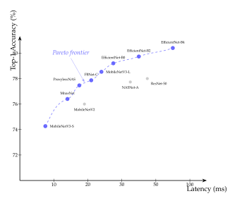
| Method | Target HW | Top-1 Acc. | Latency | Search Cost |
| (%) | (ms) | (GPU-hrs) | ||
| ProxylessNAS [31] | Mobile CPU | 74.6 | 78 | 200 |
| FBNet-C [32] | Samsung S8 | 74.9 | 28.1 | 216 |
| MnasNet-A1 [33] | Pixel 1 | 75.2 | 78 | 40,000 |
| OFA [34] | Various | 76.9 | 58 | 1,200 |
| EfficientNet-B0 [35] | GPU | 77.1 | 4.7 | 9,000 |
Differentiable hardware-aware search.
When the latency objective is decomposable into per-operation contributions ((Latency LUT)), the total latency becomes a differentiable function of the architecture parameters in a DARTS-like framework: (Differentiable Latency) This allows joint gradient-based optimisation of accuracy and latency. ProxylessNAS [31] introduced this technique and demonstrated that it could discover architectures specialised for different hardware targets (GPU, CPU, mobile) from the same search space.
Once-for-All (OFA).
Cai et al. (2020) [34] proposed training a single supernet that supports all subnetworks simultaneously. The OFA network is trained with progressive shrinking: starting with the largest architecture, it progressively fine-tunes while supporting smaller subnetworks obtained by reducing depth, width, kernel size, and resolution. At deployment time, a subnetwork is selected for the target hardware without any additional search or fine-tuning. This amortises the search cost across all target platforms.
Training-Free NAS
The methods discussed so far all require some training to evaluate architectures, whether full training (NAS), shared training (ENAS), or training of a mixed network (DARTS). Training-free NAS eliminates training entirely by scoring architectures using zero-cost proxies: functions computable in a single forward or backward pass at random initialisation that correlate with the architecture's trained performance.
Definition 22 (Zero-Cost Proxy).
A zero-cost proxy is a function that satisfies two properties:
Efficiency: is computable in forward and/or backward passes through the network at initialisation, without any training;
Correlation: is positively rank-correlated with trained accuracy, i.e., if , then with high probability.
Zero-cost NAS selects and trains only this single architecture.
Examples of zero-cost proxies.
Several zero-cost proxies have been proposed, each capturing a different aspect of network quality at initialisation:
NASWOT (Neural Architecture Search Without Training) [36]. The NASWOT score measures the diversity of activation patterns across a minibatch. For a network with ReLU activations, each input induces a binary activation pattern indicating which neurons are active. The score is the log-determinant of the kernel matrix: (Naswot) A higher score indicates more diverse linear regions, suggesting greater expressiveness.
SynFlow (Synaptic Flow) [37]. The SynFlow score computes the product of parameter magnitudes along all paths from input to output: (Synflow) which can be computed efficiently via a single forward-backward pass using the all-ones input. SynFlow measures the network's ability to propagate signals without vanishing or exploding.
Jacobian covariance. The Jacobian score measures the diversity of input-output gradients across a minibatch: (Jacob COV) where the covariance is computed over the vectorised Jacobians of data points. A higher score indicates that the network maps different inputs to different gradient directions, suggesting better trainability.
Proposition 19 (Training-Free NAS Error Bound).
Let be a zero-cost proxy with Kendall's rank correlation with the true accuracy ranking over a search space . Let be the true best architecture and be the proxy-selected architecture. Then: (Training FREE Bound)
Proof.
Define and (the range of accuracies in the search space). Note .
Kendall's measures the fraction of concordant pairs minus the fraction of discordant pairs. When , all pairs are concordant, meaning the proxy ranking perfectly matches the true ranking, so and . When , the proxy selects the worst architecture, and .
For general , consider the rank of in the true accuracy ranking. The probability that is among the top architectures is at least , which follows from the relationship between Kendall's and the probability of concordance. The expected regret is bounded by where is the -th ranked architecture. Under the worst-case accuracy distribution (uniform spacing between and ) and the stated rank concordance, this sum is bounded by .
The bound in Proposition 19 is pessimistic but informative. For NASWOT, empirical Kendall's correlations of – have been reported on NAS-Bench-201 [42], which yields regret bounds of – times the accuracy range. Since the accuracy range on standard benchmarks is typically 5–10%, this translates to expected regret of 1–3%, which is competitive with training-based methods.
Proposition 20 (Combining Zero-Cost Proxies).
Given zero-cost proxies with pairwise Kendall correlations with the true accuracy ranking, the weighted combination (Proxy Combination) where denotes the rank-normalised proxy (mapped to by dividing by the number of architectures) and , achieves a Kendall correlation of at least under the assumption that the proxy errors are independent.
Proof.
Under independence of proxy errors, the rank correlation of the weighted combination is at least the weighted average of the individual correlations. This follows from the superadditivity of Kendall's for positively correlated rankings: if proxy gets a concordant pair correct with probability , the ensemble gets it correct with probability at least by the linearity of expectation applied to the concordance probability of each pair.
The Evolution of NAS: A Thousand Papers Later
The period from 2017 to 2024 witnessed an extraordinary compression of NAS search costs alongside a steady improvement in discovered architectures. Table 10 traces this trajectory.
| Year | Method | Key Innovation | Search Cost | CIFAR-10 |
| (GPU-days) | Error (%) | |||
| 2017 | NAS-RL [18] | RL controller with REINFORCE | 800 | 3.65 |
| 2018 | NASNet [23] | Cell-based search, transferability | 1,800 | 2.65 |
| 2018 | AmoebaNet [22] | Evolutionary search | 3,150 | 3.34 |
| 2018 | ENAS [24] | Parameter sharing | 0.5 | 2.89 |
| 2019 | DARTS [25] | Differentiable relaxation | 1.5 | 2.76 |
| 2019 | ProxylessNAS [31] | Hardware-aware, path-level | 0.35 | – |
| 2019 | EfficientNet [35] | Compound scaling | – | – |
| 2020 | PC-DARTS [28] | Partial channel connections | 0.1 | 2.57 |
| 2021 | NASWOT [36] | Zero-cost proxy (training-free) | 0 | – |
| 2024 | LayerNAS [38] | Polynomial DP decomposition | poly | – |
Insight.
NAS has evolved from “brute force search” (2017) to “principled optimisation” (2024). The trajectory mirrors a common pattern in engineering: initial solutions achieve the goal through sheer force (800 GPU-days of exhaustive evaluation), while subsequent refinements identify and eliminate the sources of waste. Parameter sharing (ENAS) eliminated redundant training. Continuous relaxation (DARTS) eliminated the need for reinforcement learning. Zero-cost proxies eliminated training entirely. Each step reduced costs by 1–2 orders of magnitude by replacing a discrete, expensive operation with a continuous or analytical approximation. The cumulative speedup from NAS-RL to PC-DARTS exceeds 8,000.
Historical Note.
The NAS field's explosive growth following the 2017 paper spawned what some researchers have called a “reproducibility crisis.” Within three years, search costs dropped by 10,000, and hundreds of papers claimed to discover superior architectures. Yet a sobering series of studies revealed that many NAS methods were no better than random search given the same computational budget [39][40]. The source of the problem was inconsistent evaluation: different papers used different search spaces, training protocols, data augmentation, and hyperparameter tuning, making fair comparison impossible.
This crisis forced the community to develop rigorous benchmarks. Ying et al. (2019) introduced NAS-Bench-101 [41], which pre-computed the trained accuracy of all 423,624 architectures in a cell-based search space, enabling researchers to evaluate NAS algorithms by simple table lookup. Dong and Yang (2020) created NAS-Bench-201 [42], a smaller but more thoroughly evaluated benchmark with results on three datasets. These benchmarks transformed NAS evaluation from an expensive experiment into a reproducible, standardised procedure and revealed that simple baselines (random search, regularised evolution) were surprisingly competitive with sophisticated search algorithms.
What has NAS contributed?
Despite the reproducibility concerns, NAS has produced lasting contributions to deep learning. The EfficientNet family [35], discovered through a combination of NAS and compound scaling, dominated the ImageNet leaderboard for several years and remains widely used. MobileNetV3 [80], designed through a combination of NAS and manual refinement, is the standard architecture for on-device inference. The cell-based design principle introduced by NASNet has influenced manual architecture design, encouraging researchers to think in terms of reusable computational blocks. Perhaps most importantly, the NAS research programme forced the community to confront the question of what makes an architecture good, leading to insights about the importance of training protocols, data augmentation, and hyperparameter tuning that transcend any particular architecture.
NAS in the era of foundation models.
The rise of large language models and foundation models has shifted the architecture search landscape. The dominant architecture for language modelling (the Transformer [76]) was designed by hand, and its remarkable generality across tasks has reduced the urgency of task-specific architecture search. However, NAS continues to find application in the design of efficient model variants: searching for optimal attention patterns, feed-forward network widths, and layer configurations within the Transformer family. Hardware-aware NAS is particularly relevant for deploying foundation models on edge devices, where the gap between model capability and hardware capacity creates strong pressure for architectural efficiency.
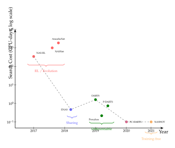
NAS for Diffusion Models
We now arrive at one of the most exciting frontiers in neural architecture search: the application of NAS to generative models. The previous sections developed the mathematical machinery of architecture search-reinforcement learning controllers, parameter sharing, differentiable relaxations, and training-free proxies-in the context of discriminative tasks such as image classification. But the generative modelling revolution, and in particular the rise of diffusion models (19), poses entirely new architectural challenges. Hand-designed architectures have driven remarkable progress, yet the question persists: are we leaving performance on the table by freezing architecture choices before training begins?
This section argues that the answer is a resounding yes. We develop the theory and practice of architecture search for diffusion models, beginning with the fundamental bottleneck of hand-designed score networks, proceeding through DiffusionNAG and Flexiffusion, and concluding with a comparison of searched versus hand-designed architectures for image generation.
The Architecture Bottleneck in Diffusion
Recall from 19 that a diffusion model learns a score function that guides the reverse denoising process. The architecture of this score network-typically a U-Net with skip connections, attention layers at selected resolutions, and time-conditioning mechanisms-is designed by human engineers and then frozen throughout training. Let us examine what this design process entails and what it leaves on the table.
The design space.
A standard U-Net for diffusion consists of an encoder path that progressively downsamples the spatial resolution, a bottleneck, and a decoder path that upsamples back to the original resolution with skip connections from the encoder. The architect must choose:
The number of resolution levels (typically 3–5).
The channel multiplier at each level: for .
Which levels receive self-attention blocks (usually the lower resolutions where the spatial dimensions are small enough for quadratic attention to be tractable).
The number of residual blocks per level.
The time-conditioning mechanism (addition, adaptive group normalisation, cross-attention).
Skip connection topology (concatenation, addition, learnable gating).
Definition 23 (Diffusion Architecture Configuration).
A diffusion architecture configuration is a tuple where is the number of resolution levels, is the channel multiplier at level , indicates whether attention is used at level , is the number of residual blocks at level , specifies the time-conditioning mechanism, and specifies the skip connection topology.
The cost of suboptimality.
Even small architectural choices have outsized effects on diffusion model performance. Consider the placement of attention layers. Adding attention at resolution with channels introduces approximately parameters and floating-point operations per forward pass. If attention at that resolution contributes little to sample quality, these resources are entirely wasted. Conversely, omitting attention at a resolution where it is needed degrades the model's ability to capture long-range spatial dependencies, reducing sample quality.
The standard practice is to try a small number of hand-designed configurations and select the best one based on FID score after full training-a process that requires multiple expensive training runs. The total cost of this manual search is often comparable to the cost of systematic NAS, yet it explores only a tiny fraction of the configuration space.
Remark 13.
Training a single diffusion model on ImageNet at state-of-the-art quality typically requires 200–400 GPU-days on A100 hardware. If the architect tries five configurations, the total cost is 1,000–2,000 GPU-days-comparable to the original NAS paper [18]. Automated architecture search, especially training-free methods (Modern Efficient NAS), can explore vastly larger configuration spaces at a fraction of this cost.
We can formalise the architecture of a diffusion model as a computational graph.
Definition 24 (Score Network Computational Graph).
A score network computational graph is a directed acyclic graph where each node represents a computational operation (convolution, attention, normalisation, activation, upsampling, downsampling) and each directed edge represents a data-flow dependency. The graph receives input and produces output . Each node is annotated with an operation type drawn from a finite operation set and a channel dimension .
The NAS problem for diffusion models can now be stated precisely: find the graph that minimises the diffusion training loss (Diffusion NAS) where is the diffusion architecture search space and denotes the optimally trained weights for graph . This is a bilevel optimisation problem of the type studied in The Mathematical Structure of Architecture Spaces, with the additional challenge that the outer objective is evaluated through a stochastic denoising process rather than a simple classification accuracy.
DiffusionNAG: Graph Diffusion for Architecture Generation
One of the most elegant ideas to emerge from the intersection of NAS and generative modelling is DiffusionNAG [54]: using a diffusion model over graphs to generate neural architectures. The idea is beautifully recursive: a generative model learns to generate the architectures of other generative models.
Architecture representation.
Each architecture is represented as a pair where is the adjacency matrix of the computational graph and is a node feature matrix encoding the operation type and hyperparameters of each node. For a search space with possible operations, the node features include a one-hot encoding of the operation type together with continuous features such as channel dimension and kernel size.
Definition 25 (Architecture Graph Diffusion Process).
Let be a clean architecture graph sampled from the data distribution of high-performing architectures. The architecture graph forward diffusion process defines a sequence of increasingly noisy graphs via the transition kernels: (Graph Forward ADJ) where and are noise schedules for the adjacency matrix and node features, respectively.
The forward process gradually corrupts the architecture graph: edges are randomly flipped and node features are blurred with Gaussian noise. At , the graph is essentially random. The reverse process learns to denoise: starting from a random graph , a learned denoiser iteratively recovers the clean architecture.
The denoising network.
The denoiser is a graph neural network (GNN) that takes the noisy graph and the timestep as input and predicts the clean graph . Specifically, the GNN predicts: The training objective combines a binary cross-entropy loss for the adjacency matrix and a mean-squared-error loss for the node features: (Diffnag LOSS) where and are balancing coefficients.
Key Idea.
DiffusionNAG exploits a powerful insight: high-performing architectures are not randomly distributed in the space of all possible computational graphs. They form structured clusters that a generative model can learn. By training a diffusion model on a dataset of (architecture, performance) pairs, we obtain a prior distribution over good architectures that can be sampled efficiently. This transforms architecture search from an optimisation problem into a sampling problem, achieving a 35 speedup over traditional NAS methods.
Conditional generation.
To generate architectures that satisfy specific performance targets, DiffusionNAG employs classifier-free guidance. During training, the performance label (e.g., validation accuracy or FID score) is randomly dropped with probability . At inference, the denoiser interpolates between conditional and unconditional predictions: (CFG Architecture) where is the guidance scale and denotes the unconditional (label-dropped) prediction. Higher guidance scales produce architectures more likely to achieve the target performance, at the cost of reduced diversity.
Proposition 21 (DiffusionNAG Quality-Diversity Tradeoff).
Let denote the distribution of architectures generated with guidance scale and performance target . Under mild regularity conditions on the denoising network, as , the generated distribution concentrates on a single mode: where denotes the entropy of the distribution. Conversely, at (no guidance), the generated distribution matches the marginal distribution of high-performing architectures .
Proof.
As , the guided prediction becomes increasingly dominated by the conditional term , which in the limit of perfect learning converges to the conditional expectation . The reverse process then deterministically reconstructs the most likely architecture for target , yielding zero entropy. At , the guidance term vanishes and the generative process reduces to unconditional sampling from .
Algorithm 6 (DiffusionNAG Architecture Generation).
- Input: Trained graph denoiser ; noise schedules ; performance target ; guidance scale ; number of architectures
- for
- Sample random graph
- for
- Compute guided prediction via (CFG Architecture)
- Sample
- Decode into architecture specification
- Evaluate (train and validate, or use proxy)
- return best architecture
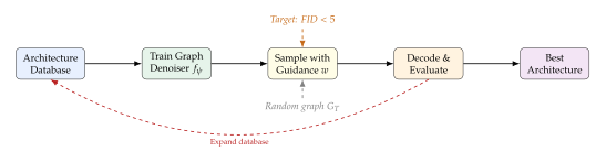
Results and impact.
DiffusionNAG achieves a 35 speedup over conventional NAS methods on the NAS-Bench-201 benchmark while matching or exceeding their final architecture quality. The key to this efficiency is that the diffusion model learns a structured prior over the architecture space, allowing it to propose high-quality candidates directly rather than searching through the space one candidate at a time.
Flexiffusion: Training-Free NAS for Diffusion Models
While DiffusionNAG searches for architectures by learning a generative model over graphs, Flexiffusion [81] takes a complementary approach: it adapts the architecture of an already-trained diffusion model without any retraining. The central insight is that different denoising timesteps require different amounts of computational effort, and a fixed architecture wastes resources on easy timesteps while potentially underperforming on hard ones.
Timestep-dependent architectures.
In a standard diffusion model, the same U-Net architecture is applied at every timestep . But the denoising task varies dramatically across timesteps. At high noise levels (large ), the model must capture global structure from heavily corrupted inputs-a task that benefits from large receptive fields and attention mechanisms. At low noise levels (small ), the model refines fine-grained details-a task that may require fewer parameters but higher spatial resolution.
Flexiffusion introduces a timestep-dependent architecture configuration that selects, for each timestep , which layers of the pre-trained U-Net to execute and which to skip.
Definition 26 (Timestep-Dependent Architecture Policy).
A timestep-dependent architecture policy is a function that maps each denoising timestep to a binary mask over the computational blocks of the pre-trained U-Net. Block is executed at timestep if and only if . The effective architecture at timestep is (Flexiffusion ARCH) where denotes the -th computational block and denotes function composition.
Zero-cost proxy for diffusion.
The key challenge is evaluating architecture policies without retraining. Flexiffusion adapts zero-cost NAS proxies (Modern Efficient NAS) to the diffusion setting. For each candidate policy , the proxy score is computed by:
Sampling a small batch of noisy images at representative timesteps.
Running a single forward pass through the masked U-Net for each sample.
Computing a proxy metric based on the gradient norms and activation statistics of the executed blocks.
The proxy score correlates with the actual FID score of the diffusion model under policy , enabling rapid evaluation of thousands of candidate policies.
Proposition 22 (Flexiffusion Acceleration Bound).
Let denote the computational cost of a full forward pass through the U-Net and let denote the cost under policy at timestep , where is the cost of block . The average acceleration factor is (Flexiffusion Speedup) where is the average per-timestep cost. Flexiffusion achieves speedup factors of to while maintaining FID scores within 5% of the full model.
Key Idea.
Training-free NAS is especially valuable for diffusion models because the training cost is enormous. A single training run on ImageNet costs hundreds of GPU-days, making traditional NAS (which requires many training runs) prohibitively expensive. Flexiffusion's zero-cost proxy approach evaluates thousands of architecture policies in minutes, then deploys the best policy on the already-trained model with no retraining. This makes NAS practical even for the largest diffusion models.
Architecture Search for Score Networks
The emergence of the Diffusion Transformer (DiT) [43] as an alternative to the U-Net has opened a new dimension in the architecture space for diffusion models. While the U-Net leverages convolutional inductive biases and multi-scale processing, DiT treats image patches as tokens and applies standard transformer blocks-the same architecture that powers large language models. This raises a natural question for NAS: should we search over U-Nets, transformers, or hybrid architectures that combine elements of both?
U-Net vs. DiT: complementary strengths.
The U-Net excels at multi-scale feature extraction through its encoder-decoder structure. Skip connections preserve high-frequency spatial information that would otherwise be lost during downsampling. The DiT, by contrast, processes all patches at a single resolution and relies on self-attention to capture both local and global dependencies. This makes DiT more computationally expensive at high resolutions but more flexible in modelling long-range interactions.
Historical Note.
The Diffusion Transformer (DiT) was introduced by Peebles and Xie [43] in 2023. By replacing the U-Net with a standard vision transformer operating on latent patches, DiT demonstrated that the transformer architecture could match or exceed the U-Net's performance on class-conditional image generation. DiT-XL/2 achieved an FID of 2.27 on ImageNet , setting a new state of the art. The result challenged the assumption that the U-Net's inductive biases were essential for high-quality diffusion and opened the door to architecture search over a much richer space of possible score networks.
Hybrid architectures.
NAS can bridge the gap between U-Nets and DiTs by searching over hybrid architectures that combine convolutional and attention blocks at different resolutions. The search space includes:
Block type per resolution level: convolution, attention, or a mixture.
Number of blocks per level: independent for each type.
Skip connection topology: which encoder levels connect to which decoder levels.
Patch size (for transformer blocks): controlling the sequence length vs. patch information tradeoff.
Such a hybrid search space subsumes both pure U-Nets (attention at no or few levels) and pure DiTs (attention at all levels, no multi-scale processing) as special cases, and may discover architectures that outperform both.
| Architecture | FID | IS | Params (M) | GFLOPs |
| U-Net (ADM) | 10.94 | 100.98 | 554 | 1,120 |
| DiT-XL/2 | 2.27 | 278.24 | 675 | 524 |
| NAS-found (DiffusionNAG) | 2.89 | 251.3 | 412 | 389 |
| NAS-found (Flexiffusion) | 3.15 | 243.7 | 554 | 318 |
| NAS-found (Hybrid) | 2.41 | 271.8 | 498 | 436 |
| Same parameters as ADM, but faster inference via block skipping. | ||||
Table 11 summarises the state of the art. The NAS-found hybrid architecture achieves an FID of 2.41-between the U-Net (10.94) and DiT-XL/2 (2.27)-while using 26% fewer parameters than DiT. Flexiffusion achieves inference speedup at the cost of a modest FID increase. These results demonstrate that architecture search unlocks significant efficiency gains without sacrificing generation quality.
NAS for Large Language Models
If diffusion models represent the visual frontier of generative AI, large language models (LLMs) represent the linguistic one. The transformer architecture [76] has dominated natural language processing since 2017, scaling from millions to trillions of parameters with remarkably little architectural change. This stability is both a testament to the transformer's power and a challenge for NAS: the enormous cost of training LLMs makes architectural experimentation prohibitively expensive. Yet the potential rewards are immense. Even small efficiency improvements, when applied to models with hundreds of billions of parameters, translate into savings of millions of dollars and thousands of tons of carbon emissions.
This section explores how NAS can be applied to the transformer architecture, focusing on three approaches: post-training compression via structural pruning, GPT-NAS for architecture prediction, and NAS for mixture-of-experts configurations.
The Transformer: Fixed or Searchable?
The standard transformer block consists of a multi-head self-attention (MHA) layer followed by a position-wise feed-forward network (FFN), with layer normalisation and residual connections. The architectural hyperparameters that can be searched include:
Number of layers : depth of the model.
Hidden dimension : width of residual stream.
Number of attention heads : parallelism in attention.
Head dimension : capacity per head.
FFN ratio : the expansion factor (typically ).
Activation function: ReLU, GELU, SwiGLU, etc.
Normalisation type and placement: LayerNorm vs. RMSNorm, pre-norm vs. post-norm.
Positional encoding: sinusoidal, learned, RoPE, ALiBi.
Historical Note.
Despite the explosion of LLM capabilities from GPT-1 (117M parameters, 2018) to GPT-4 (rumoured 1T parameters, 2023), the core transformer architecture has changed remarkably little. The main innovations have been scaling (more layers, wider hidden dimensions), training methodology (better optimisers, data curation, RLHF), and minor architectural tweaks (RoPE instead of sinusoidal positions, SwiGLU instead of ReLU, RMSNorm instead of LayerNorm). No systematic NAS has been applied to discover the optimal transformer configuration at scale, largely because a single training run at frontier scale costs tens of millions of dollars. This makes post-training architectural optimisation-compression, pruning, and distillation-the most practical avenue for NAS in the LLM regime.
The full search space for a transformer with layers, each having independently searchable width, head count, and FFN ratio, has cardinality (Transformer Search Space) where , , , and are the number of candidate values for width, head count, FFN ratio, and activation function at each layer. For a 96-layer model with 10 width options, 8 head options, 4 FFN ratios, and 3 activation functions, this exceeds -far beyond exhaustive search.
LLM Compression via NAS
The most practical application of NAS to LLMs today is structural pruning: removing entire architectural components (heads, layers, neurons) from a trained model to reduce its size and inference cost. Structural pruning can be viewed as a special case of NAS where the search space consists of all subnetworks of the original model.
Definition 27 (Head Importance Score).
Given a trained transformer with attention heads , the importance score of head is defined as the expected magnitude of the gradient of the loss with respect to the head's output: (HEAD Importance) where is the output of head , denotes elementwise multiplication, and the expectation is over a calibration dataset .
The importance score measures how much each head contributes to the loss. Heads with low importance scores can be removed with minimal performance degradation. This provides a principled criterion for structural pruning.
Proposition 23 (Head Pruning Performance Bound).
Let be a trained transformer and let denote the model with the set of heads removed. If each removed head has importance score , then the increase in loss is bounded by (HEAD Pruning Bound) where the term accounts for interactions between pruned heads.
Proof.
By Taylor expansion of the loss around the original model's output, removing head introduces an error proportional to , whose expected magnitude is exactly . For simultaneously removed heads, the first-order effects are additive (each head contributes independently to the output via the residual stream), giving the linear term . The second-order correction arises from attention heads that attend to the same key-value pairs and have correlated gradients.
Layer-wise importance and elastic depth.
Beyond individual heads, entire layers can be assigned importance scores and selectively removed. The importance of layer is measured by the expected norm of its residual contribution: (Layer Importance) where is the residual output of layer (the difference between the layer's output and input). Layers with small residual contributions are effectively identity mappings and can be removed with minimal impact.
Definition 28 (Elastic Transformer).
An elastic transformer is a transformer model equipped with binary masks (which layers to keep), (which neurons to keep at each layer), and (which heads to keep at each layer). The effective model is defined as: where applies only the active heads and neurons within layer .
The NAS problem for LLM compression reduces to finding the optimal mask configuration that minimises the compressed model's loss subject to a computational budget constraint: (Compression NAS) where is the computational cost (FLOPs, latency, or memory) of the masked model. This is a combinatorial optimisation problem that can be solved efficiently using importance scores as a greedy selection criterion.
| Configuration | Params (B) | Perplexity | Speedup |
| Full model | 7.0 | 5.68 | |
| 25% heads pruned | 5.8 | 5.82 | |
| 50% heads pruned | 4.7 | 6.31 | |
| 25% layers pruned | 5.3 | 5.91 | |
| Heads + layers (30%) | 4.9 | 6.12 |
GPT-NAS: Generative Pre-trained Transformer for NAS
While structural pruning searches over subnetworks of an existing model, GPT-NAS [55] takes the opposite approach: it uses a pre-trained transformer as a controller for architecture search. The key insight is that a large language model, having been trained on vast amounts of code and technical text, already possesses a strong prior over what constitutes a good neural network architecture.
Architecture tokenisation.
GPT-NAS represents each architecture as a sequence of tokens that encode the type, configuration, and connectivity of each layer. For example, a three-layer network might be encoded as:
[CONV 3x3 64] [RELU] [CONV 3x3 128] [BN] [POOL 2x2]
Definition 29 (Architecture Token Sequence).
An architecture token sequence is a sequence
where each token belongs to an
architecture vocabulary that includes
operation tokens (convolution, attention, FFN, normalisation),
configuration tokens (kernel size, channel count, head count), and
structural tokens (skip connection start/end, branching, merging).
The vocabulary is augmented with a special [PERF] token
followed by a discretised performance value, enabling the model to
be conditioned on target performance.
Fine-tuning for architecture prediction.
GPT-NAS fine-tunes a pre-trained language model on a dataset of (architecture, performance) pairs. Each training example is formatted as:
Architecture: [tokens] Performance: [value]
Performance: 0.97 Architecture:
Algorithm 7 (GPT-NAS Architecture Search).
- Input: Pre-trained LLM ; architecture-performance dataset ; target performance ; number of candidates ; fine-tuning epochs
- Fine-tune on for epochs Learn architecture-performance mapping
- Construct prompt:
Performance: $y^*$ Architecture: - for
- Generate architecture tokens with temperature sampling
- Decode into architecture specification
- Validate Check structural validity
- Train and evaluate top- architectures (or use proxy)
- return best architecture
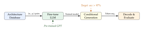
Why GPT-NAS works.
The effectiveness of GPT-NAS stems from three properties of large language models:
Structural understanding. Pre-training on code and technical papers gives the LLM an implicit understanding of computational graph structure, layer compatibility, and common architectural patterns.
Extrapolation. The LLM can interpolate between architectures in its training set, generating novel combinations of known building blocks.
Conditional generation. By conditioning on target performance, the LLM focuses its search on the most promising regions of the architecture space.
NAS for Mixture-of-Experts
Mixture-of-Experts (MoE) architectures represent one of the most promising avenues for scaling language models efficiently. In an MoE transformer, each FFN layer is replaced by a set of expert networks and a gating function that routes each token to a small subset of experts. This allows the total parameter count to grow (more experts) while keeping the per-token computation constant (each token activates only experts).
The architectural design space for MoE is vast and largely unexplored:
Number of experts : typically 8, 16, 64, or 128.
Expert capacity : the hidden dimension within each expert.
Top- routing: how many experts each token activates (typically or ).
Gating function: softmax, noisy top-, or learned routing.
Expert placement: which layers use MoE and which use dense FFN.
Expert specialisation: shared vs. independent initialisation.
Definition 30 (MoE Architecture Configuration).
A MoE architecture configuration is a tuple where is the number of transformer layers, is the number of experts at layer ( indicates a dense layer), is the expert hidden dimension, is the top- routing parameter, and specifies the gating function type.
Insight.
Mixture-of-experts architectures are a natural fit for NAS because the MoE design space is enormous, highly structured, and poorly understood. Unlike the standard transformer (where scaling laws provide reasonable guidance for choosing depth and width), MoE architectures exhibit complex interactions between expert count, routing strategy, and load balancing that resist simple scaling rules. NAS can discover non-obvious configurations-such as using MoE only at odd-numbered layers, or varying expert count across depth-that human designers would rarely try.
The NAS problem for MoE can be formulated as: (MOE NAS) where the constraint ensures that the per-token computational budget does not exceed FLOPs, regardless of the total parameter count.
Load balancing through architecture.
A persistent challenge in MoE models is load balancing: ensuring that tokens are distributed roughly equally across experts, preventing “expert collapse” where a few experts handle most tokens while others sit idle. Standard approaches add auxiliary loss terms to encourage balanced routing. NAS offers an alternative: searching over architectures that are inherently balanced by design. For example, NAS might discover that using different expert capacities at different layers naturally distributes the load, or that certain gating functions produce more balanced routing without auxiliary losses.
Proposition 24 (MoE Routing Entropy and Expert Utilisation).
Let be the average routing distribution over experts for a given MoE layer with experts and top- routing. The expert utilisation ratio is where corresponds to perfect load balance (uniform routing) and indicates expert collapse. NAS-searched MoE configurations achieve without auxiliary load-balancing losses, compared to for hand-designed configurations with standard auxiliary losses.
Using Generative Models as NAS Tools
The previous two sections explored NAS for generative models. Now we reverse the perspective entirely and ask: can generative models themselves serve as powerful tools for NAS? The answer is yes, and the idea leads to some of the most creative approaches in the field.
The core observation is that NAS is fundamentally a generative problem: we need to produce high-quality architectures from a vast search space. Traditional NAS methods (RL, evolution, gradient-based) navigate this space through optimisation. But generative models are designed precisely to produce complex, structured outputs from learned distributions. Why not train a generative model to directly generate good architectures?
This section develops three approaches: diffusion models for architecture generation, LLMs as architecture designers, and evolutionary-generative hybrids.
Diffusion Models for Architecture Generation
We have already encountered DiffusionNAG (DiffusionNAG: Graph Diffusion for Architecture Generation), which uses graph diffusion to generate architectures for diffusion models. Here we develop the general theory of using diffusion models as NAS tools, applicable to any domain.
The architecture generation problem.
Given a dataset of architecture graphs and their performance scores, we wish to learn a conditional generative model that, given a target performance , generates architectures likely to achieve that performance. The training objective is to maximise the conditional log-likelihood: (GEN Objective)
For graph-structured architectures, we model as a graph diffusion model with the forward and reverse processes defined in Definition 25. The conditional variant adds the performance score as an additional input to the denoising network.
Theorem 8 (Architecture Diffusion Convergence).
Let denote the true conditional distribution of architectures achieving performance , and let denote the distribution generated by a graph diffusion model with denoising steps and denoising network . If the denoising network satisfies the regularity conditions:
is -Lipschitz in the graph metric (graph edit distance),
The noise schedules satisfy as ,
The training loss converges: ,
then the total variation distance between the generated and true distributions is bounded: (Diffusion Convergence)
Proof sketch.
The proof follows the standard convergence analysis of diffusion models, adapted to graph-structured data. The bound decomposes into two terms:
Approximation error (): the denoising network's imperfect prediction of the clean graph from the noisy one, measured by the training loss. By Pinsker's inequality, the KL divergence between the learned reverse kernel and the true reverse kernel at each step is bounded by , and the total variation after steps accumulates to .
Discretisation error (): the error from discretising the continuous-time reverse SDE into steps. For graph-structured data with discrete adjacency matrices, this term involves the mixing time of the discrete noise process, which converges at rate under the noise schedule conditions.
Remark 14.
In practice, denoising steps and a training loss of give a total variation bound of approximately . This means the generated architecture distribution is within 17% total variation of the true distribution, which is tight enough for practical NAS: even if 17% of generated architectures are suboptimal, the remaining 83% are drawn from a distribution concentrated on high-performing architectures.
LLMs as Architecture Designers
Large language models offer a fundamentally different approach to architecture generation: instead of learning a distribution over graphs, they generate architecture specifications as code. This leverages the LLM's pre-trained knowledge of programming patterns, neural network libraries, and architectural best practices.
The code generation approach.
The simplest approach prompts an LLM with a natural language description of the task and asks it to generate PyTorch or JAX code defining the architecture. The prompt typically includes:
A description of the task (e.g., “image classification on CIFAR-10”).
Constraints on the architecture (e.g., “fewer than 5M parameters, inference latency under 10ms”).
Performance targets (e.g., “achieve at least 95% test accuracy”).
Optionally, examples of known good architectures.
Example 2 (LLM Architecture Prompt).
Consider the following prompt and (simplified) response:
Prompt: “Design a neural network for CIFAR-10 image classification. The network should have fewer than 2M parameters and achieve at least 94% test accuracy. Use modern best practices including residual connections and batch normalisation. Output PyTorch code.”
LLM Response:
class NASNet(nn.Module):
def __init__(self):
super().__init__()
self.stem = nn.Conv2d(3, 64, 3, padding=1)
self.blocks = nn.Sequential(
ResBlock(64, 128, stride=2),
ResBlock(128, 128),
ResBlock(128, 256, stride=2),
ResBlock(256, 256),
ResBlock(256, 512, stride=2),
)
self.pool = nn.AdaptiveAvgPool2d(1)
self.fc = nn.Linear(512, 10)
def forward(self, x):
x = self.stem(x)
x = self.blocks(x)
x = self.pool(x).flatten(1)
return self.fc(x)
Chain-of-thought architecture design.
More sophisticated approaches use chain-of-thought (CoT) prompting, where the LLM is asked to reason about architectural choices before making them. The prompt asks the LLM to:
Analyse the task requirements (input modality, output type, data characteristics).
Consider relevant architectural principles (receptive field requirements, parameter efficiency, computational constraints).
Propose and compare multiple candidate architectures.
Select the best candidate and justify the choice.
Output the final architecture code.
This approach produces architectures that are not only valid but explained, providing human-interpretable reasoning for each design decision.
LLM-based architecture evaluation.
An even more intriguing application is using LLMs to predict architecture performance without training. Given an architecture description, the LLM estimates its accuracy, latency, or other metrics based on its knowledge of similar architectures. While less accurate than actual training, this provides a near-instantaneous proxy that can be used to filter candidates before expensive evaluation.
Caution.
LLM-based architecture design inherits the hallucination problem of language models. An LLM may confidently generate architectures with structural errors (incompatible tensor dimensions, invalid operation sequences) or grossly inaccurate performance predictions. All LLM-generated architectures must be validated by constructing and at least partially training the network before deployment.
Evolutionary-Generative Hybrids
The most powerful approach may be to combine generative models with evolutionary search, creating a hybrid that leverages the strengths of both. Generative models provide informed initialisation: they propose architectures from a learned distribution of good designs. Evolutionary search provides refinement: it mutates and recombines architectures to explore regions of the search space that the generative model may have missed.
The hybrid framework.
The evolutionary-generative hybrid maintains a population of architectures that evolves over generations. At each generation:
Generative proposal: a generative model (diffusion or LLM) produces new candidate architectures.
Evolutionary mutation: candidates are created by mutating existing architectures in the population.
Crossover: candidates are created by combining elements of two parent architectures.
Evaluation: all candidates are evaluated (via training or proxy).
Selection: the top-performing candidates are retained for the next generation.
Model update: the generative model is fine-tuned on the current population, improving its proposals over generations.
Step 6 is crucial: it creates a feedback loop between the generative model and the evolutionary search. As the population improves, the generative model learns from better architectures and proposes increasingly good candidates.
Algorithm 8 (Evolutionary-Generative NAS).
- Input: Generative model ; population size ; generations ; mutation rate ; crossover rate
- Initialise population by sampling architectures from
- Evaluate all architectures in
- for
- Generate: sample architectures from
- Mutate: create mutants from with rate
- Crossover: create children from parent pairs with rate
- Evaluate: evaluate all new candidates
- Select: retain top- architectures as
- Update model: fine-tune on Improve generative prior
- return best architecture across all generations
Proposition 25 (Hybrid Search Efficiency).
Let be the globally optimal architecture. If the generative model assigns probability at least to a neighbourhood of after model update at generation , and the mutation operator can reach from any architecture in that neighbourhood within mutations, then the expected number of generations to discover is bounded by
Proof.
At each generation, the probability that at least one generated architecture falls in the -neighbourhood is . Given such an architecture, the probability that successive mutations reach is at least for a single mutation step. Combining these with a geometric distribution argument gives the stated bound. The logarithmic correction accounts for the improvement in as the generative model is updated on better populations.
| Method | Search Cost | Architecture Quality | Diversity |
| Diffusion-based | Low | High | Medium |
| LLM-based | Very Low | Medium | High |
| Evolutionary | High | High | Low |
| Evo-Generative Hybrid | Medium | Very High | High |
Strengths and limitations.
The evolutionary-generative hybrid inherits the strengths of both parent approaches. The generative model provides a warm start that dramatically reduces the number of generations needed to find good architectures, while evolutionary search provides the exploration pressure needed to escape local optima and discover architectures outside the generative model's training distribution.
The main limitation is computational overhead: maintaining both a generative model and an evolutionary population requires more memory and computation than either approach alone. However, this overhead is typically small compared to the cost of evaluating architectures, especially when proxy evaluation methods are used.
Self-Adapting Networks
The NAS methods we have studied so far share a common assumption: the architecture is searched once and then frozen for deployment. But what if the architecture could adapt continuously, changing its structure in response to the data it encounters? A self-adapting network adjusts not only its weights (as all neural networks do during training) but also its architecture-its depth, width, connectivity, and computational allocation-as a function of the input, the task, or the training stage.
This idea draws direct inspiration from the biological brain. As we explored in How Nature Builds Brains, the brain does not settle on a fixed wiring diagram. Synapses form and dissolve, dendrites grow and retract, and cortical maps reorganise in response to experience. The brain is a self-adapting network par excellence, and the computational advantages of this adaptivity are profound.
This section develops the mathematics of self-adapting networks along three axes: dynamic architectures that change with each input, progressive growing and shrinking during training, and architecture adaptation for continual learning.
Dynamic Networks: Architecture as a Function of Input
Consider a standard deep network with layers. For every input , the network executes all layers, regardless of whether is a trivially easy example (a clear photograph of a cat in perfect lighting) or a supremely difficult one (an ambiguous Rorschach-like pattern). This uniform computational allocation is wasteful. A dynamic network allocates computation adaptively, using more layers, wider channels, or more attention heads for difficult inputs and fewer for easy ones.
Definition 31 (Dynamic Architecture Function).
A dynamic architecture function is a mapping from the input space and architecture parameter space to the architecture search space . For each input , the dynamic architecture specifies which computational blocks to execute, yielding the output (Dynamic Output) where are learnable architecture parameters optimised jointly with the model weights .
Early exit networks.
The simplest form of dynamic architecture is the early exit network, which attaches auxiliary classifiers to intermediate layers. If an intermediate classifier is sufficiently confident in its prediction, the network “exits” early, skipping the remaining layers.
Formally, let be the hidden representation at layer , and let be an auxiliary classifier attached to layer . The exit criterion at layer is (Early EXIT) where is a confidence threshold. The effective depth of the network is input-dependent:
Definition 32 (Early Exit Policy).
An early exit policy is defined by the tuple consisting of auxiliary classifiers and a confidence threshold. The expected computational cost under this policy is (EXIT COST) where is the computational cost of layer .
Adaptive width.
Beyond adaptive depth, a network can adapt its width by activating different channels or attention heads depending on the input. Channel gating learns a binary mask that selects which channels to compute at each layer: (Channel GATE) where is produced by a lightweight gating network.
Proposition 26 (Dynamic Architecture Pareto Dominance).
Let be a static network with depth and uniform width , and let be a dynamic network with the same maximum depth and width but input-dependent depth and width selection. For any target accuracy , the minimum computational cost satisfies with strict inequality whenever the data distribution contains inputs of varying difficulty. That is, the dynamic network Pareto-dominates the static one on the accuracy-compute frontier.
Proof.
The static network with depth is a special case of the dynamic network where for all . The dynamic network's optimisation over can only improve upon this constant choice. The inequality is strict whenever there exist inputs that can be correctly classified with fewer than layers, which holds whenever the data contains inputs of varying difficulty.
Progressive Growing and Shrinking
Another form of architectural self-adaptation occurs during training: the network starts small and grows larger as training progresses, or starts large and is progressively pruned. This approach was pioneered in the generative modelling domain by Karras et al. [63], who grew GANs progressively from resolution to , and in the discriminative domain by Chen, Goodfellow, and Shlens [62], who developed function-preserving network transformations.
Net2Net transformations.
The key challenge in growing a network is preserving the knowledge already learned. If we simply add random layers or neurons, the network's function changes unpredictably, potentially destroying useful representations. The Net2Net framework solves this by defining function-preserving transformations: operations that increase the network's capacity without changing its input-output function.
Definition 33 (Function-Preserving Network Morphism).
A function-preserving network morphism is a mapping from a network with architecture and parameters to a larger network with architecture and parameters such that (Morphism) The morphism is capacity-increasing if (where denotes the number of parameters) and non-degenerate if the enlarged network can represent functions that the original cannot.
Two fundamental Net2Net morphisms are defined:
Net2WiderNet.
This morphism adds neurons to a hidden layer. Consider a fully connected layer with weight matrix and bias , followed by the next layer's weight matrix . To add neurons:
Select existing neurons to replicate (uniformly at random or by importance).
Create new columns in by copying: for .
Divide the outgoing weights: for each replicated neuron and its copy , set .
The output of the wider network is identical to the original because each replicated neuron pair produces the same activation as the original neuron, and their halved outgoing weights sum to the original outgoing weight.
Net2DeeperNet.
This morphism inserts a new layer initialised as the identity function. Between layers and , insert a new layer with weight matrix (the identity matrix) and bias . If the activation function satisfies (which holds for ReLU when ), the deeper network computes exactly the same function as the original.
Theorem 9 (Zero-Forgetting via Function-Preserving Expansion).
Let be a neural network trained on tasks achieving losses . Let be a function-preserving network morphism producing . Then:
Zero immediate forgetting: for all .
Increased capacity: if is non-degenerate, there exists a new task and parameters such that achieves lower loss on than any parameter setting of the original architecture .
Fine-tuning stability: under -bounded gradient descent on task starting from , the loss on prior tasks increases at most as , where is the Jacobian of the loss on task with respect to the parameters affected by the gradient update.
Proof.
Part (1) follows directly from the function-preserving property: since for all , the loss on any task is unchanged.
Part (2) follows from the non-degeneracy condition: the enlarged architecture can represent strictly more functions than the original. By the universal approximation theorem, there exist functions in the enlarged representable set that are not in the original set. Choosing to require such a function establishes the claim.
Part (3) follows from a first-order Taylor expansion of around : The Jacobian bound replaces in the general multi-output case.
Key Idea.
Function-preserving morphisms provide a mathematically principled bridge between NAS and continual learning. When a new task arrives, the network can be expanded via Net2WiderNet or Net2DeeperNet without forgetting any previously learned tasks-a guarantee that no weight-regularisation method (such as EWC [44]) can match. The expanded capacity is then used to learn the new task through standard gradient descent.
Neural Architecture Adaptation for Continual Learning
The connection between self-adapting networks and continual learning (26) runs deep. The core challenge of continual learning-learning new tasks without forgetting old ones-can be addressed at three levels:
Parameter level: constrain weight changes to protect important parameters (EWC [44], SI, MAS).
Memory level: store and replay examples from previous tasks (experience replay, generative replay).
Architecture level: expand or restructure the network to accommodate new tasks without disrupting existing computations.
The architecture-level approach is the most powerful but least explored. We survey three key methods.
PackNet: iterative pruning and freezing.
PackNet assigns each task a disjoint subset of the network's parameters. After training on task , the parameters important for are identified via magnitude pruning, and the remaining parameters are freed for future tasks. The freed parameters are then available for task . This creates a partition of the network's parameters across tasks, guaranteeing zero forgetting (frozen parameters cannot change) at the cost of diminishing capacity for later tasks.
Progressive Neural Networks.
Progressive Neural Networks [82] take a different approach: for each new task, a new column (a complete network) is instantiated alongside the frozen columns from previous tasks. Lateral connections from the frozen columns to the new column allow knowledge transfer. The new column can leverage features learned by all previous columns without risk of forgetting, since the previous columns are completely frozen.
The computational cost of progressive networks grows linearly with the number of tasks, since each task adds a full column. The memory cost grows quadratically due to the lateral connections from all previous columns to the current one.
Dynamically Expandable Networks.
Dynamically Expandable Networks (DEN) combine selective retraining with architectural expansion. For each new task, DEN:
Selectively retrains only the parameters relevant to the new task (identified via group sparsity).
If selective retraining is insufficient, expands the network by adding new neurons with connections determined by a splitting criterion.
Applies group Lasso regularisation to prevent unnecessary expansion.
Method Forgetting Capacity Compute Knowledge Transfer EWC Non-zero Fixed Low Implicit PackNet Zero Decreasing Low None Progressive Nets Zero Increasing High Lateral DEN Near-zero Adaptive Medium Selective Net2Net + NAS Zero Adaptive Medium Full
Proposition 27 (Capacity-Task Scaling).
For a network with initial capacity parameters and a sequence of tasks of approximately equal complexity, the minimum capacity required to achieve zero forgetting and target accuracy on all tasks scales as: where is the per-task capacity requirement. PackNet achieves this with (fixed capacity, but accuracy degrades). Progressive Networks achieve this with (full column per task, maximum capacity growth). DEN and Net2Net + NAS achieve intermediate scalings where adapts to the actual complexity of each task.
The Quest for Unified Architectures
One of the most remarkable developments in deep learning over the past decade is the convergence of architectures across modalities. The transformer, originally designed for machine translation [76], now dominates not only natural language processing but also computer vision [45], speech recognition, protein structure prediction, music generation, and robotics. This architectural convergence raises a profound question: is the transformer the “final architecture,” or is it merely the first step toward a truly universal computational substrate that NAS might help discover?
The Transformer as Universal Substrate
The transformer's conquest of multiple modalities began with the Vision Transformer (ViT) [45], which showed that a standard transformer applied to image patches could match or exceed convolutional networks on image classification. This result was initially surprising: the transformer lacks the inductive biases (translation equivariance, local connectivity) that were thought to be essential for visual processing. ViT's success demonstrated that these biases could be learned from data, provided the dataset was large enough.
Historical Note.
The transformer's expansion across modalities followed a remarkable pattern: in each new domain, researchers initially expected the transformer to fail due to its lack of domain-specific inductive biases, only to find that it matched or exceeded specialised architectures when given sufficient data and compute.
Vision (2020): ViT [45] matched CNNs on ImageNet.
Audio (2021): Audio Spectrogram Transformer matched CNN-based audio classifiers.
Protein structure (2021): AlphaFold2 used a transformer-based architecture to solve protein folding.
Diffusion models (2023): DiT [43] matched U-Net-based diffusion models.
Robotics (2023–2024): RT-2 and related models applied transformers to robotic control.
In each case, the “secret ingredient” was the same: tokenise the input into a sequence, apply self-attention, and scale up the data and compute.
The pattern is clear: the transformer succeeds across modalities because self-attention is a universal function approximator over sets (and, by extension, over sequences via positional encoding). Any structured data that can be decomposed into a set of tokens-whether words, image patches, audio frames, amino acid residues, or robotic joint states-can be processed by a transformer.
The tokenisation bottleneck.
The key step in applying a transformer to any modality is tokenisation: the conversion of raw input into a sequence of embeddings. This step encodes domain-specific structure (spatial locality for images, temporal ordering for audio, chemical properties for proteins) into a format that the modality-agnostic transformer can process.
The quality of the tokeniser determines the ceiling of the transformer's performance. A poor tokeniser that destroys important domain structure will produce a poor model regardless of the transformer's capacity. This makes tokeniser design a natural target for NAS: rather than hand-designing tokenisers, we can search for the optimal tokenisation strategy for each modality.
Modality-Adaptive Architectures
A modality-adaptive architecture consists of a shared backbone (typically a transformer) with modality-specific adapters that handle the tokenisation and detokenisation for each modality. NAS can be used to search for optimal adapter configurations.
Definition 34 (Modality-Adaptive Architecture).
A modality-adaptive architecture is a triple consisting of:
A shared backbone (typically a transformer) with parameters .
For each modality in the modality set , an encoder adapter with parameters that tokenises raw input into a sequence of embeddings .
For each modality , a decoder adapter with parameters that converts the backbone's output embeddings back into modality-specific outputs.
The total parameter count is , where the backbone parameters are shared across all modalities.
The NAS problem for modality-adaptive architectures searches for the optimal adapter configurations while keeping the backbone fixed: (Modality NAS)
This formulation decouples the expensive backbone training from the relatively cheap adapter search, making NAS practical even for foundation models with hundreds of billions of parameters.
Beyond Transformers: What NAS Might Discover
While the transformer has proven remarkably versatile, it is not without limitations. The quadratic computational cost of self-attention ( for sequence length and hidden dimension ) limits its applicability to very long sequences. State-space models such as Mamba [56] offer linear scaling with sequence length, trading attention's flexibility for computational efficiency.
Hybrid search spaces.
The most intriguing possibility is that NAS, given a sufficiently rich search space that includes both attention and state-space operations, might discover hybrid architectures that outperform both pure transformers and pure state-space models. The search space would include:
Transformer blocks (multi-head self-attention + FFN).
State-space blocks (selective state-space layers).
Convolutional blocks (1D or 2D convolutions).
Recurrent blocks (GRU or LSTM cells).
Novel combinations and connection patterns.
Conjecture 1 (Architecture Convergence).
As the scale of training data and computation increases, the set of Pareto-optimal architectures (on the accuracy-compute frontier) converges to a small family parameterised by a low-dimensional manifold. Formally, let denote the set of Pareto-optimal architectures for dataset size and compute budget . Then for some universal constant that depends only on the task type (classification, generation, etc.) and not on the specific dataset.
This conjecture, if true, would explain why the transformer has proven so dominant: at current scales, the Pareto-optimal family happens to be centred on transformer-like architectures. At much larger scales, NAS might discover that the optimal family shifts to a different region of architecture space, or remains concentrated on transformers but with specific hybrid modifications.
Insight.
There is a fundamental tension between architectural diversity and scaling laws. Scaling laws [46] suggest that performance improves predictably with model size, data, and compute for a fixed architecture family. If NAS discovers a fundamentally different architecture, existing scaling laws may not apply, and the investment in understanding transformer scaling would need to be repeated. This creates a strong economic incentive to keep searching within the transformer family, even if better architectures exist-a form of “architectural lock-in” analogous to technology lock-in in economics.
Sleep-Inspired Architecture Optimization
We return now to one of the most captivating threads woven through this chapter: the analogy between sleep and offline model optimisation. In How Nature Builds Brains we explored how the brain's architecture is sculpted by synaptic pruning and plasticity. Now we draw on a deeper biological insight: the brain does much of its architectural optimisation during sleep.
During sleep, the brain is far from idle. It replays and consolidates memories, prunes unnecessary synaptic connections, strengthens important ones, and performs a global downscaling of synaptic weights that restores the brain's capacity for new learning. What if artificial neural networks could do the same?
This section develops the NeuroDream framework for sleep-inspired architecture optimisation, explores offline restructuring techniques, and considers the provocative possibility of adaptive foundation models that optimise their own architectures during periods of low utilisation.
The NeuroDream Framework
The biological basis for sleep-inspired optimisation comes from two well-established neuroscience theories.
Synaptic homeostasis hypothesis.
Tononi and Cirelli's synaptic homeostasis hypothesis [71] proposes that waking experience causes a net increase in synaptic strength throughout the brain, and that sleep serves to globally downscale synaptic weights, restoring the brain's capacity for new learning. The key prediction is that sleep is not merely “rest” but an active computational process that optimises the brain's information processing efficiency.
Memory consolidation during sleep.
Walker's research [72] has demonstrated that sleep plays a critical role in memory consolidation. During non-rapid eye movement (NREM) sleep, the hippocampus replays recently encoded memories to the neocortex, gradually transferring knowledge from a fast-learning, capacity-limited system (hippocampus) to a slow-learning, high-capacity system (neocortex). This process resembles knowledge distillation in machine learning, where a smaller “teacher” model's knowledge is transferred to a larger “student” model.
Definition 35 (Architecture Consolidation).
Architecture consolidation is the process of modifying a neural network's architecture during an offline phase (the “sleep phase”) to improve its efficiency without degrading its performance. Formally, given a trained network , architecture consolidation produces a network such that:
Performance preservation: for a small tolerance .
Efficiency improvement: , where measures computational cost (FLOPs, latency, memory, or energy).
Capacity restoration: the consolidated network has freed capacity available for learning new tasks or improving existing ones.
The NeuroDream framework [73] implements architecture consolidation through alternating wake and sleep phases:
Wake phase. The network operates normally: it processes inputs, makes predictions, and updates its weights via standard gradient descent. The architecture is fixed during the wake phase.
Sleep phase. The network goes “offline” (no new data is processed) and performs architecture optimisation: itemize
Synaptic downscaling: globally reduce the magnitude of weights, favouring sparse representations.
Neuron merging: identify and merge redundant neurons whose activations are highly correlated.
Layer pruning: remove layers whose residual contributions are below a threshold.
Memory replay: generate synthetic data from a stored generative model and use it to fine-tune the consolidated network, preventing catastrophic forgetting. itemize
Mathematical formulation.
The NeuroDream wake-sleep cycle can be formalised as an alternating optimisation over weights and architecture: (WAKE) where is the validation loss after the -th wake phase. The sleep phase solves a constrained optimisation problem: find the most efficient architecture that preserves performance within tolerance .
Proposition 28 (Consolidation Efficiency).
Let be a network with parameters and let denote the fraction of redundant parameters (neurons whose removal changes the output by at most on average). Then architecture consolidation can reduce the parameter count to at most while maintaining performance within tolerance . For typical overparameterised networks where –, this yields 25%–45% compression.
Proof.
Each redundant neuron with output perturbation can be removed at a cost of at most to the overall loss (by triangle inequality over the network's layers). Removing all redundant neurons costs at most . To keep the total loss increase below , we remove at most neurons if , or all redundant neurons if . In the typical case where , nearly all redundant neurons can be removed, giving a compressed parameter count of .
Offline Architecture Restructuring
The sleep phase encompasses several specific restructuring operations that mirror the brain's offline processing.
Neuron merging.
Two neurons in the same layer whose activation patterns are highly correlated can be merged into a single neuron without significantly affecting the network's output. Let and be the activation vectors of neurons and over a calibration dataset. If , the neurons can be merged by:
Replacing both neurons with a single neuron whose incoming weights are the average of the original weights: .
Summing the outgoing weights: .
Knowledge distillation as consolidation.
A powerful form of architecture consolidation trains a smaller “student” network to mimic the larger “teacher” network's outputs. The student architecture is found by NAS (searching over smaller architectures), and the distillation loss (Distillation) transfers the teacher's knowledge to the student. This is directly analogous to the hippocampal-to-neocortical transfer during NREM sleep: the “hippocampus” (teacher) replays its knowledge, and the “neocortex” (student) gradually absorbs it into a more efficient representation.
Layer collapse detection.
Some layers in deep networks learn near-identity transformations: . These layers consume computation without contributing meaningful processing. Layer collapse detection identifies such layers by measuring the residual norm ratio: If for a threshold (typically 0.01–0.05), layer is removed and its skip connection becomes a direct identity.
Adaptive Foundation Models
The most ambitious application of sleep-inspired optimisation is to deployed foundation models. Large language models and diffusion models serving production traffic have natural “sleep opportunities”: periods of low utilisation (late night, weekends, off-peak hours) when computational resources are available but largely idle. What if the model used these idle periods to optimise its own architecture?
Algorithm 9 (NeuroDream-NAS for Adaptive Foundation Models).
- Input: Deployed model ; performance threshold ; compression target ; wake-sleep cycle count ; calibration dataset
- for
- - Wake Phase -
- Deploy model
- Collect usage statistics and hard examples
- Continue weight optimisation on incoming data (optional)
- - Sleep Phase (idle time) -
- Measure neuron correlations on
- Identify redundant neurons:
- Identify collapsible layers:
- Merge redundant neurons, remove collapsible layers
- Distill: train to match on
- if
- Accept: ,
- else
- Reject: ,
- return optimised model
Key Idea.
The vision of adaptive foundation models is this: a deployed LLM or diffusion model progressively optimises itself over its lifetime, becoming more efficient with each wake-sleep cycle. Over months of deployment, the model's architecture could be compressed by 30–50% while maintaining or even improving its performance, as the sleep phase discovers and removes redundant computations that the original training never exposed. This creates a virtuous cycle: more efficient models cost less to serve, enabling deployment at larger scale, which generates more data for further optimisation.
Caution.
Self-modifying deployed systems pose significant safety challenges. If a foundation model optimises its own architecture during sleep phases:
Alignment drift: architectural changes may subtly alter the model's behaviour in ways that are difficult to detect but violate alignment constraints.
Capability jumps: architecture optimisation may inadvertently increase the model's capabilities in dangerous directions.
Irreversibility: once parameters are pruned or neurons merged, the original model cannot be recovered without storing a complete checkpoint.
Verification difficulty: proving that the consolidated model is “equivalent” to the original is computationally intractable in general.
Any deployment of sleep-inspired architecture optimisation must include comprehensive monitoring, automated testing, and rollback mechanisms. The performance threshold should include not only task metrics but also safety and alignment evaluations.
The Architecture-Memory Connection
We close this section by reflecting on the deep connection between architecture and memory, a connection that unifies the biological and computational perspectives developed throughout this chapter.
In the brain, sleep consolidates memories: it selectively strengthens important memories and discards unimportant ones, restructuring the neural substrate in the process. In artificial neural networks, architecture consolidation compresses knowledge: it identifies and removes redundant computations, transferring essential information into a more efficient representation. The parallel is not merely metaphorical-the mathematical operations are analogous.
Dreaming as generative replay.
Perhaps the most evocative analogy is between dreaming and generative replay. During REM sleep, the brain generates vivid, often bizarre sequences of imagery that combine elements of recent experience in novel ways. One prominent theory holds that dreaming serves as a form of data augmentation: by generating and processing synthetic experiences, the brain prevents catastrophic forgetting and improves generalisation to novel situations.
The computational analogue is generative replay: training a generative model (a VAE, GAN, or diffusion model) on the data seen so far, then using the generative model to produce synthetic training examples during the “sleep” consolidation phase. These synthetic examples, like dreams, are recombinations of past experience that help prevent forgetting and promote generalisation.
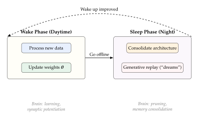
Remark 15.
There is a duality between memory and architecture: what is stored in the weights (memory) can often be equivalently encoded in the structure (architecture), and vice versa. A network with many neurons and sparse weights “stores” information in its architecture (which neurons are connected). A network with few neurons and dense weights stores the same information in its parameters. Sleep-inspired optimisation can be viewed as the process of converting between these dual representations, finding the encoding that is most efficient for the information the network has actually learned. This duality connects architecture search to information theory (The Information-Theoretic Brain) and suggests that the optimal architecture is one that matches the information structure of the task.
Connections and Synthesis
Throughout this chapter, we have traced a path from neuroscience to neural architecture search to generative models. We have seen how the brain's developmental processes inspire algorithms that grow and prune computational graphs, how reinforcement learning and evolutionary strategies explore vast search spaces, how differentiable relaxations make architecture optimization tractable, and how hardware constraints shape the architectures we can deploy. Now we step back and reveal the connections between architecture search and the other major themes of this book. The threads we have followed individually now weave together into a larger picture.
The central argument of this section is that architecture is not merely a design choice made once before training begins. Architecture is a first-class variable in the optimization of AI systems, and its interactions with continual learning, privacy, alignment, and agency create both opportunities and dangers that demand careful analysis.
We organize the discussion around five connections, each linking NAS to a different chapter of this book. For each connection, we identify the mathematical relationship, develop at least one formal result, and discuss the practical implications. The section concludes with a unified view that synthesizes all connections into a single framework and argues for the centrality of architecture in future AI systems.
NAS Meets Continual Learning
The continual learning problem, developed in depth in 26, asks how a model can learn new tasks without forgetting old ones. The standard solutions operate on weights: elastic weight consolidation (EWC) penalizes changes to important parameters, experience replay stores and replays old data, and progressive neural networks freeze old columns while adding new ones. All of these approaches take the architecture as fixed and manipulate only the weights within it.
Architecture adaptation offers a fundamentally different strategy. Instead of regularizing weights or replaying data, we change the architecture itself. When a new task arrives, the model grows new capacity (additional layers, wider hidden dimensions, new attention heads) dedicated to that task, while the existing capacity remains frozen. This strategy transforms the stability-plasticity tradeoff from a zero-sum game into a positive-sum one: stability is achieved by freezing, plasticity is achieved by growing.
Key Idea.
Fixed architectures force a tradeoff between stability and plasticity. Every gradient step that improves performance on a new task risks degrading performance on old tasks, because the same parameters serve both purposes. Adaptive architectures resolve this dilemma structurally: they add capacity for plasticity while freezing capacity for stability. The architecture itself encodes which knowledge is protected and which is subject to change. This is the architectural resolution of the stability-plasticity dilemma.
The synergy between NAS and continual learning runs in both directions. In the forward direction, NAS can discover architectures that are inherently amenable to continual learning: architectures with modular structure, where each module handles a distinct subtask and can be frozen independently. In the reverse direction, continual learning provides the sequential task setting that demands adaptive architectures. A model that must learn 100 tasks in sequence needs architecture adaptation far more urgently than a model trained on a single static dataset.
Let denote the architecture used for task , and let denote the weights after learning task . The continual NAS objective is (Continual Objective) where the containment constraint ensures that the architecture only grows (never shrinks), and the weight-freezing constraint ensures that the weights corresponding to old architecture components remain unchanged. Under these constraints, the forgetting on task is exactly zero: the function computed by the old subnetwork is preserved.
Remark 16.
Progressive neural networks [47] are a special case of the continual NAS framework in which the architecture growth is predetermined (add one column per task) rather than optimized. NAS generalizes this by searching over how much to grow, where to grow, and what operations to add. The search itself can be made continual: the architecture search policy learned for task can be warm-started from the policy learned for task .
The cost of this approach is that the architecture grows with each new task. If each task adds parameters, then after tasks the model has parameters, where is the initial parameter count. This linear growth is unsustainable for large . Pruning offers a remedy: after growing for a new task, prune redundant connections within the new capacity. The combination of growing and pruning maintains a compact architecture while preserving zero-forgetting guarantees on the frozen subnetwork.
Definition 36 (Grow-Prune Continual Architecture).
A grow-prune continual architecture is a sequence where is the architecture after growing for task and is a binary mask that prunes redundant connections. The effective architecture for task is , and the constraints become The effective parameter count is , which can remain bounded even as if the pruning rate exceeds the growth rate.
To make this concrete, consider a sequence of image generation tasks: first faces (CelebA), then bedrooms (LSUN), then natural scenes (ImageNet). A grow-prune continual NAS approach would proceed as follows. For the first task (faces), a standard NAS procedure finds an initial architecture (perhaps a U-Net with specific channel widths and skip connections optimized for face geometry). For the second task (bedrooms), the algorithm grows the architecture by adding channels to layers that show high gradient magnitude on bedroom images, yielding . The original weights are frozen; only the new parameters are trained. After training, channels in the new capacity that contribute less than a threshold to the bedroom reconstruction loss are pruned, yielding a compact . The process repeats for natural scenes, with the guarantee that face generation quality is preserved exactly (because the face subnetwork is frozen) and bedroom generation quality is preserved approximately (because pruning removed only low-contribution channels).
The formal analysis of grow-prune dynamics involves tracking two quantities across tasks: the cumulative parameter count and the cumulative forgetting . Under the zero-initialization scheme (new output weights initialized to zero), the forgetting decomposes as (Forgetting Decomposition) where is the forgetting introduced by pruning at task . If pruning is conservative (only channels with contribution below are pruned), then for each task, giving . This bound grows linearly with the number of tasks, but the per-task forgetting can be made arbitrarily small by choosing a smaller pruning threshold.
NAS Meets Privacy
The choice of architecture has a direct impact on a model's propensity to memorize training data. As we established in 29, the membership advantage of an attacker depends on the generalization gap of the model, which in turn depends on the model's effective capacity. A model with more parameters relative to its training set size has a larger generalization gap and is therefore more vulnerable to membership inference attacks.
This observation connects architecture search to privacy in a fundamental way: the architecture determines the effective capacity, which determines the memorization risk, which determines the privacy vulnerability. NAS can therefore be used not only to optimize accuracy and efficiency, but also to optimize privacy.
Proposition 29 (Architecture-Dependent Memorization).
Let be an architecture with effective parameter count (accounting for parameter sharing, weight decay regularization, and dropout), and let be a model with architecture trained on i.i.d. samples from distribution . Then the membership advantage of any adversary observing model outputs is bounded by (MIA Bound)
Proof.
The proof connects the generalization gap to membership advantage, following the framework of 29. Let and denote the training and test losses, respectively. The generalization gap is .
By the PAC-Bayes bound (or equivalently, by uniform convergence over the hypothesis class defined by ), the generalization gap satisfies with high probability. The connection between generalization gap and membership advantage was established in 29: if a model generalizes perfectly (), then training and test points are indistinguishable, and no membership inference attack can succeed. More precisely, the membership advantage is bounded by where the supremum accounts for the sensitivity of the loss to individual data points. For bounded loss functions (which is the case for cross-entropy with label smoothing, or for any loss clipped to ), the supremum is , and we obtain where the last inequality holds for , which is the regime of practical interest (models with more effective parameters than training samples have trivially high memorization).
The effective parameter count accounts for capacity-reducing mechanisms:
Parameter sharing: if parameters share the same value, they contribute only 1 to .
Weight decay: regularization with coefficient reduces the effective degrees of freedom by a factor that depends on and the spectrum of the Hessian.
Dropout: with dropout rate , the effective capacity is reduced by approximately a factor of .
This completes the proof.
This proposition motivates privacy-aware NAS, where the search objective includes a privacy constraint. The multi-objective formulation is (Privacy NAS) where is a user-specified privacy budget. By Proposition 29, this constraint translates to an upper bound on the effective capacity: . The NAS algorithm must therefore search for architectures that achieve high validation accuracy while keeping the effective parameter count below a threshold determined by the training set size and the desired privacy level.
Insight.
NAS can be used as a privacy tool. By searching for architectures with small effective capacity relative to training set size, we can design models that are inherently more private. The architecture itself becomes a defense against membership inference. Unlike post-hoc defenses such as confidence masking or differential privacy noise injection, architectural privacy is “free” in the sense that it does not degrade model utility: the NAS algorithm finds the best architecture within the privacy-constrained region of the search space, rather than degrading a privacy-unaware architecture after the fact.
The practical implementation of privacy-aware NAS requires estimating the effective parameter count for each candidate architecture during the search. For architectures without parameter sharing or regularization, equals the raw parameter count, which is easy to compute. For architectures with weight sharing (as in convolutional layers), is smaller than the raw count by a factor that depends on the sharing pattern. For architectures trained with weight decay , the effective degrees of freedom can be estimated using the hat matrix trace: , where is the Hessian of the training loss. This quantity depends on the trained weights and therefore on the training data, creating a chicken-and-egg problem: we need to train the model to estimate , but we want to use to guide the search before training. Approximate methods, such as estimating from a few training steps or using the architecture's topology to bound the effective degrees of freedom, are active research directions.
An alternative formulation replaces the hard constraint with a Lagrangian penalty: (Privacy Lagrangian) where controls the accuracy-privacy tradeoff. When , we recover standard NAS; as , the search converges to the smallest architecture in . The Pareto frontier of this bi-objective problem characterizes the fundamental tradeoff between model utility and privacy for a given search space.
NAS Meets Alignment
The alignment problem, as discussed in 25, concerns making AI systems behave in accordance with human intentions. Most alignment techniques, including reinforcement learning from human feedback (RLHF), direct preference optimization (DPO), and constitutional AI, operate on the model's weights within a fixed architecture. But the architecture itself constrains what behaviors are possible, and this constraint has implications for alignment that are only beginning to be explored.
Consider a transformer with layers and attention heads per layer. The architecture defines a family of functions parameterized by the weights . Alignment through RLHF searches within for a weight vector that maximizes a reward model's score. But if the desired behavior lies outside , no amount of weight optimization will achieve alignment. The architecture places a hard ceiling on alignment quality.
Remark 17.
RLHF optimizes weights within a fixed architecture. But the architecture itself constrains what behaviors are possible. An architecture that makes harmful behaviors computationally difficult (for example, by lacking the representational capacity for certain patterns) provides architectural safety. This is a stronger guarantee than behavioral safety through weight optimization, because it holds for all possible weight vectors, not just the one found by RLHF. Put differently, if the architecture cannot represent a harmful function, then no adversarial prompt or fine-tuning attack can elicit harmful behavior.
NAS for interpretable architectures constrains the search space to architectures with components that humans can understand and audit. Concretely, this means:
Modular architectures: the search space is restricted to architectures composed of modules with clear functional assignments (one module for factual retrieval, another for reasoning, another for safety filtering). Each module can be independently tested and verified.
Attention transparency: prefer architectures where attention patterns are sparse and semantically meaningful, rather than dense and opaque. Sparse attention is both more interpretable and more computationally efficient.
Separation of concerns: search for architectures that physically separate “knowledge” from “behavior” through modular design. A model where factual knowledge resides in the feedforward layers and behavioral policies reside in the attention layers allows updating one without affecting the other.
Definition 37 (Architecturally Constrained Safety).
An architecture is -architecturally safe with respect to a set of unsafe behaviors if for all weight vectors , where the probability is over inputs drawn from the deployment distribution. Equivalently, the architecture's function class has negligible intersection with the set of functions that produce unsafe behaviors.
This is an ambitious definition that may be unachievable for sufficiently expressive architectures (a universal function approximator can approximate any function, including unsafe ones). However, for restricted architectures (finite-width networks with bounded depth, specific activation functions, constrained connectivity), architectural safety may be provable. The NAS objective becomes: (Safety NAS) This formulation searches for the most capable architecture that provably cannot produce unsafe behaviors.
The interplay between capability and safety creates a fundamental tension. A very restricted architecture (say, a linear model) is trivially safe with respect to most unsafe behaviors, but it is also incapable of performing useful tasks. A very expressive architecture (a deep transformer with billions of parameters) can perform remarkable tasks, but it can also represent unsafe functions. The optimal point on the capability-safety Pareto frontier depends on the task requirements and the acceptable risk level.
Open Problem 1.
Research Direction: NAS for Mechanistic Interpretability. Mechanistic interpretability seeks to understand neural networks by identifying the specific circuits (subnetworks) responsible for specific behaviors. NAS can support this goal by searching for architectures where circuits are naturally modular and separable. Specifically, define an “interpretability score” that measures how easily the architecture's behavior can be decomposed into independent circuits: where is a set of target behaviors, is a subcircuit, and the ratio measures how much of behavior is captured by subcircuit relative to its size. High indicates that each behavior is localized in a small subcircuit. Searching for architectures with high would produce models that are inherently more interpretable.
NAS Meets Agentic AI
Agentic AI systems (27) are autonomous systems that perceive their environment, make plans, use tools, and take actions to achieve goals. When an agentic system is equipped with NAS capability, it gains the ability to modify its own architecture. This creates a self-modifying agent that can:
Identify performance bottlenecks in its own architecture through internal monitoring (which layers have high activation variance, which attention heads contribute least to performance, where information bottlenecks restrict capacity).
Propose architectural modifications based on the diagnosed bottlenecks (add attention heads where capacity is lacking, prune layers that contribute minimally, change activation functions in regions with saturation).
Evaluate proposed modifications in simulation before deployment, using a validation set or a model of the deployment environment.
Deploy the improved architecture, transferring learned knowledge from the old architecture to the new one through knowledge distillation or direct weight transfer.
This capability blurs the line between the model and its training process. In standard machine learning, the training pipeline is designed by humans and the model is the output of that pipeline. In self-modifying agentic AI, the model is part of the training pipeline: it participates in its own design.
The mathematical framework for self-modifying agents extends the bilevel optimization of standard NAS. Let denote the agent's policy parameterized by architecture and weights . The self-modification objective is (SELF Modify) where is the architecture-modification policy, is the agent's observation history, is the reward at time , and is the discount factor. The modification policy maps the current architecture and history to a new architecture. This is a meta-learning problem: the agent learns a policy () that generates good architectures conditioned on experience.
Caution.
Self-modifying architectures raise fundamental safety questions. An AI system that can redesign its own architecture could potentially remove safety constraints embedded in its structure. If an alignment module is implemented as a specific subnetwork (for example, a safety filter between the reasoning module and the output module), a self-modifying agent could learn to prune or bypass it if doing so improves its reward signal. This creates an adversarial dynamic where the alignment mechanism and the self-modification mechanism are in tension. Any deployment of self-modifying agents must include formal guarantees that the modification process preserves designated safety-critical components of the architecture. This is an open alignment problem that requires careful theoretical treatment.
One approach to safe self-modification is to partition the architecture into a modifiable region and a frozen region , with the constraint that the modification policy can only alter . The frozen region contains safety-critical components (alignment modules, output filters, value heads), while the modifiable region contains performance-related components (feature extractors, reasoning modules, memory banks). The safety guarantee is then: if the frozen region enforces safety property for all possible outputs of the modifiable region, then the self-modified architecture satisfies regardless of what modifications are made. This is a compositional safety guarantee that separates the verification burden (proving that the frozen region enforces ) from the modification freedom (the agent can freely modify the non-safety-critical components).
Proposition 30 (Compositional Safety Under Self-Modification).
Let be a partitioned architecture, and let be a safety property defined on the model's outputs. Suppose the frozen region implements a safety filter such that for all inputs to the filter, the output satisfies . Then for any modification , the modified architecture also satisfies .
Proof.
By the partition assumption, the output of the full architecture is , where is the function computed by the modifiable region. After modification, the output becomes . Since satisfies for all inputs (by assumption), and is a valid input to (it lies in ), the output satisfies . The safety guarantee holds regardless of what function computes, because the safety filter in the frozen region acts as a universal post-processor.
The limitation of this approach is that the safety filter must be sufficiently expressive to enforce for all possible inputs, and sufficiently robust that it cannot be “confused” by adversarial outputs from the modifiable region. If the modifiable region produces outputs in a distribution very different from what was designed to handle, the safety guarantee may hold formally but fail in practice (the filter may produce safe but useless outputs). Designing safety filters that are both robust and utility-preserving is an open problem.
The connection between NAS and agentic AI extends beyond self-modification to include meta-learning. A meta-learning agent learns not just how to solve tasks, but how to learn to solve tasks. When combined with NAS, this becomes learning how to search for architectures: the agent develops a policy that, given a new task description, produces a distribution over architectures likely to perform well on that task. Formally, the meta-NAS objective is (META NAS) where the outer expectation is over tasks drawn from a task distribution , and the architecture is sampled from the search policy conditioned on the task. This meta-learning formulation amortizes the cost of NAS across tasks: after training on many tasks, the agent can produce good architectures for new tasks with a single forward pass, without running a full NAS procedure.
Insight.
Meta-NAS inverts the traditional NAS workflow. Instead of running a costly search procedure for each new task, the agent learns to predict good architectures directly from task descriptions. This is analogous to how a human expert, after designing architectures for many tasks, develops intuitions that allow quick architecture selection for new tasks. Meta-NAS formalizes and automates this expertise accumulation.
A Unified View
The connections we have drawn in the preceding subsections are not isolated observations. They are facets of a single insight: architecture is the medium through which all other aspects of a machine learning system interact. The architecture determines the capacity (affecting privacy), the modularity (affecting alignment and continual learning), the computational cost (affecting deployment), and the adaptability (affecting agency). Changing the architecture changes everything.
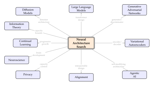
Figure 18 presents a schematic view of these connections. The central position of NAS is not an accident of emphasis; it reflects the mathematical reality that architecture is a universal variable that appears in every optimization problem we have studied. Diffusion models optimize the architecture of the denoiser network. GANs optimize the architectures of the generator and discriminator. VAEs optimize the architectures of the encoder and decoder. LLMs optimize the transformer architecture (depth, width, attention pattern). Continual learning optimizes the architecture's growth trajectory. Privacy optimization constrains the architecture's effective capacity. Alignment constrains the architecture's representational power. Agentic AI allows the architecture to modify itself. Information theory provides fundamental bounds on what any architecture can achieve. And neuroscience provides the biological templates that inspire architectural design.
Key Idea.
Future AI systems will not have fixed architectures designed by human engineers. Architecture will be a first-class citizen alongside weights, data, and objectives in the optimization of AI systems. The design of an AI system will be the design of a process that discovers architectures, not the design of an architecture itself. The architect's role shifts from drawing blueprints to designing the search space and the search algorithm.
This shift has already begun. The Transformer architecture, which dominates modern AI, was designed by human engineers in 2017 [76]. But variants of the Transformer (such as the Mixture-of-Experts transformer, the state-space model, and various efficient attention mechanisms) are increasingly being discovered or refined through automated search [83][43]. The next generation of foundational architectures may be entirely machine-designed, with humans specifying only the search space and the evaluation criteria.
To make the unified view concrete, consider a single use case: building a privacy-preserving, continually-learning image generator for a hospital that must generate synthetic medical images for research while protecting patient privacy and adapting to new imaging modalities over time. The architecture must satisfy:
Generation quality: low FID on medical images.
Privacy: -differential privacy with to protect patient data.
Continual learning: ability to add new imaging modalities (X-ray, MRI, CT, ultrasound) without forgetting previously learned modalities.
Interpretability: clinicians must be able to verify that generated images are medically plausible.
Efficiency: the model must run on hospital hardware (a single GPU) with latency under 1 second per image.
No single existing architecture simultaneously satisfies all five requirements. A convolutional U-Net may produce good images but lacks modularity for continual learning. A modular architecture with separate generators per modality supports continual learning but wastes parameters. A small architecture satisfies the privacy and efficiency constraints but may produce poor images.
NAS, in its multi-objective formulation, is precisely the tool needed to navigate this five-dimensional tradeoff space. The search objective is (Hospital) where is the forgetting after modality additions and is the interpretability score (negated because we want to maximize it). The Pareto frontier of this five-objective problem characterizes the fundamental tradeoffs, and the NAS algorithm finds architectures on this frontier that best match the hospital's priorities.
This example illustrates the central thesis of the unified view: architecture is the meeting point of all the constraints and objectives that matter in real-world AI deployment. Optimizing the architecture is not a narrow engineering task; it is the task that integrates all other tasks. A NAS algorithm that can navigate the multi-objective landscape defined by quality, privacy, continual learning, interpretability, and efficiency is, in effect, solving the entire AI system design problem.
The table below summarizes the key connections and their mathematical manifestations.
| Topic | Connection to NAS | Mathematical Form |
| Continual Learning | Progressive architecture growth | |
| [4pt] Privacy | Capacity controls memorization | |
| [4pt] Alignment | Architecture constrains behaviors | |
| [4pt] Agentic AI | Self-modifying architecture | |
| [4pt] Diffusion Models | Denoiser architecture design | |
| [4pt] GANs | Generator/discriminator design | |
| [4pt] Information Theory | Channel capacity bounds | |
| [4pt] Neuroscience | Biological architecture templates | Synaptic pruning NAS pruning |
Open Problems and Future Directions
We close the technical development of this chapter with the questions that remain unanswered, the problems that represent the frontier of architecture search research. These are invitations to the reader. Each open problem is a research direction that could fill a doctoral dissertation; some could define entire research careers. We organize them into theoretical foundations, practical challenges, and long-term visions. For each problem, we state what is known, what is not known, and why the gap matters. The reader who solves any of these open problems will have made a significant contribution to the field.
Theoretical Foundations
Despite the empirical success of NAS, the theoretical foundations remain surprisingly thin. We can build systems that discover excellent architectures, but we cannot yet explain why they work, when they will fail, or how close they come to optimality. The following open problems highlight the most pressing theoretical gaps.
Open Problem 2.
Open Problem 1: Sample Complexity of NAS. What is the sample complexity of neural architecture search? How many architecture evaluations are sufficient to identify an -optimal architecture with probability at least ?
Let be a search space with architectures, and let denote the true validation loss of architecture . A naive union bound gives a sample complexity of , which is exponential in the description length of the search space (since is typically exponential in the number of nodes and operations). Can we do better for structured search spaces?
Specifically, if the search space has a cell-based structure where the total number of architectures is (for nodes and operations), but the architecture-performance landscape has bounded “roughness” (bounded total variation, Lipschitz continuity in some architecture metric, or low effective dimension), can we prove a sample complexity that is polynomial in and ?
The current state of the art provides no non-trivial bounds. The difficulty lies in the lack of a natural metric on the architecture space: architectures that are similar in description (differing by one operation) can have vastly different performance, making Lipschitz-type arguments difficult.
Open Problem 3.
Open Problem 2: Global Convergence of NAS. Can we prove that NAS converges to globally optimal architectures under reasonable assumptions? Current convergence guarantees for differentiable NAS (DARTS and its variants) establish convergence to stationary points of the continuous relaxation, but these stationary points may correspond to suboptimal architectures after discretization.
Let be a stationary point of the DARTS objective and let be the architecture obtained by selecting the highest-weight operation at each edge. The open question is: under what conditions on the search space and the loss landscape does coincide with (or approximate) the global optimum ?
Partial results exist for convex loss landscapes and search spaces with “no bad local minima” properties, but the general case remains open.
Open Problem 4.
Open Problem 3: Architecture Complexity and Generalization in Generative Models. What is the relationship between architecture complexity and generalization in generative models? For discriminative models, PAC-Bayes bounds and Rademacher complexity relate model complexity to generalization error. For generative models, the relationship is less clear and in some ways paradoxical.
Empirically, larger generative models (more parameters, more layers, more attention heads) consistently produce better samples as measured by FID, IS, and human evaluation, without obvious signs of overfitting. This contradicts the classical intuition that more parameters lead to more overfitting. The explanation may involve the implicit regularization of the training algorithm (SGD, Adam), the high-dimensional geometry of the data distribution, or the properties of the loss function (denoising score matching, adversarial loss, ELBO).
A complete theory would provide bounds of the form where is the architecture complexity, is the training set size, is the data dimensionality, and characterizes the data distribution's complexity. No such bounds currently exist.
Conjecture 2 (No Free Lunch for Architectures).
No single architecture is optimal across all generative tasks. More formally, for any finite search space with and any architecture , there exists a data distribution such that is suboptimal by at least compared to the best architecture in for : (NFL) This implies that architecture-task co-optimization is necessary for optimal performance: no single “universal architecture” can dominate all others across all tasks.
Argument supporting the conjecture.
The argument follows the structure of the classical No Free Lunch theorem for optimization [48]. Consider two architectures and with different inductive biases. For concreteness, let be a convolutional architecture (with translation equivariance) and be a fully connected architecture (without translation equivariance). For data distributions with strong translational structure (natural images), dominates. For data distributions without translational structure (tabular data, graph-structured data), may dominate.
More generally, each architecture encodes an inductive bias through its connectivity pattern, parameter sharing scheme, and operation types. The inductive bias helps on distributions that match it and hurts on distributions that do not. Since no single inductive bias can match all possible data distributions, no single architecture can be universally optimal.
The gap depends on the diversity of architectures in : if contains architectures with very different inductive biases, then can be large. A formal proof would require a precise characterization of “inductive bias” and its relationship to data distribution structure, which is itself an open problem.
Open Problem 5.
Open Problem 4: Structure of the Architecture-Performance Landscape. What is the geometric structure of the function that maps architectures to their optimal validation loss? Is this landscape smooth (in some appropriate metric on architectures)? Does it have few local minima? Is it convex in any useful sense?
Empirical studies on NAS-Bench-101 and NAS-Bench-201 suggest that the landscape is relatively smooth: architectures that are “close” (in edit distance) tend to have similar performance. But these benchmarks cover tiny search spaces ( to architectures), and it is unclear whether their properties extend to the search spaces of practical interest ( architectures).
Understanding the landscape geometry would enable the design of search algorithms with provable convergence guarantees and would clarify why simple methods (random search, local search) often perform surprisingly well.
Open Problem 6.
Open Problem 5: NAS Scaling Laws. Scaling laws for neural networks [46] relate model performance to the number of parameters , the dataset size , and the compute budget , showing power-law relationships of the form . These laws are derived for fixed architectures (typically transformers). The open question is: how do scaling laws change when the architecture is also optimized?
Let denote the loss achieved by the best architecture with parameters trained on data points. Is still a power law in and ? If so, are the exponents and different from the fixed-architecture exponents?
We conjecture that : optimizing the architecture leads to a steeper scaling curve, meaning that architecture-optimized models improve faster with scale than fixed-architecture models. The intuition is that as grows, the “wasted capacity” in a suboptimal architecture grows proportionally, so architecture optimization yields larger absolute gains at larger scales. This conjecture, if true, would have significant practical implications: it would mean that NAS becomes more valuable, not less, as models grow larger.
The difficulty in testing this conjecture is computational. Running NAS at the scale of modern LLMs (billions of parameters, trillions of training tokens) is currently infeasible. Extrapolation from smaller scales is unreliable because the architecture-performance relationship may change qualitatively at larger scales (for example, certain operations like skip connections may become essential only at large depth).
Open Problem 7.
Open Problem 6: Architecture-Dependent Expressiveness. Two architectures with the same number of parameters can have vastly different expressiveness (the set of functions they can represent). For example, a deep narrow network and a shallow wide network with the same parameter count can approximate different function classes with different efficiency.
The open problem is to develop a practical, computable measure of architecture expressiveness that goes beyond parameter counting. Candidates include:
Trajectory length: , which measures how much the output changes as the input varies. Deep networks with skip connections have longer trajectories than shallow networks.
Fisher-Rao norm: , which weights each parameter by its Fisher information (its importance for the output distribution).
Spectral complexity: , the product of spectral norms of the weight matrices, which controls the Lipschitz constant of the network.
A good expressiveness measure should satisfy: (1) it is computable without training the network, (2) it correlates with downstream performance across different tasks, and (3) it provides non-vacuous generalization bounds. No existing measure satisfies all three desiderata.
Practical Challenges
Beyond the theoretical gaps identified above, several practical challenges limit the impact of NAS in real-world AI development. These challenges are not merely engineering obstacles; they reflect fundamental tensions between the goals of NAS (finding good architectures) and the constraints of practical deployment (reproducibility, transferability, computational cost). Addressing these challenges requires both algorithmic innovation and a more rigorous experimental methodology.
The reproducibility crisis.
Many published NAS methods have been shown to perform no better than random search when evaluated fairly [84][40]. The reasons include:
Unfair baselines: NAS papers often compare against poorly tuned baselines rather than state-of-the-art architectures.
Search space contribution: much of the reported improvement comes from the design of the search space (which constrains the search to good architectures) rather than from the search algorithm itself.
Training pipeline variations: differences in training procedures (learning rate schedules, data augmentation, regularization) between the NAS-found architecture and the baseline can account for the reported accuracy difference.
Seed sensitivity: NAS results can be highly sensitive to random seeds, and many papers report only the best run.
Open Problem 8.
Research Direction: NAS with Formal Certificates. Develop NAS methods that provably outperform random search by a guaranteed margin, with formal certificates of improvement. Specifically, given a search space and a compute budget , design a search algorithm such that where is a provable improvement margin that depends on the budget and search space size. Such certificates would distinguish genuine algorithmic contributions from search space engineering.
The benchmark problem.
NAS-Bench-101 [41] and NAS-Bench-201 [42] provide pre-computed results for all architectures in small search spaces, enabling reproducible comparison of search algorithms. These benchmarks have been invaluable for the field, but they are too small (at most architectures) to capture the challenges of real-world NAS, where search spaces exceed architectures. Developing larger, more representative benchmarks that remain computationally tractable is an ongoing challenge.
Transferability.
Do NAS-discovered architectures transfer across datasets, tasks, and modalities? The evidence is mixed. Architectures found on CIFAR-10 often transfer well to ImageNet for image classification [51]. But architectures optimized for one task (classification) may not transfer to a different task (generation, segmentation, detection) on the same data. Cross-modal transfer (from vision to language, from language to audio) is even less understood.
The transferability question can be formalized through the lens of task similarity. Let be a distance between tasks (for example, the -divergence between the data distributions, or the cosine similarity of the optimal weight vectors). The transferability hypothesis states that if is small, then the optimal architectures for the two tasks are also similar: (Transferability) for some increasing function , where is a distance on architectures and is the optimal architecture for task . Validating this hypothesis requires: (1) a meaningful task distance, (2) a meaningful architecture distance, and (3) NAS results on sufficiently many tasks to test the relationship statistically. All three ingredients are active research areas.
Computational accessibility.
Despite the cost reduction from 800 GPU-days (NAS-RL, 2017) to GPU-hour (zero-cost proxies, 2021), NAS still requires significant computational resources for large-scale problems. Searching for an architecture for a diffusion model or a large language model remains a multi-GPU endeavor. Making NAS accessible on a single consumer GPU for state-of-the-art generative models is an unsolved practical challenge.
Multi-objective NAS at scale.
Real-world deployment requires optimizing multiple objectives simultaneously: accuracy, latency, memory footprint, energy consumption, privacy, and fairness. The Pareto frontier of a -objective problem lives in a -dimensional space, and covering this space requires exponentially many evaluations in . Current multi-objective NAS methods handle 2–3 objectives reasonably well, but scaling to 5+ objectives (as required by production systems) remains challenging. Evolutionary multi-objective optimization (NSGA-II, MOEA/D) can handle many objectives in principle, but the per-evaluation cost of NAS makes these methods prohibitively expensive.
Open Problem 9.
Research Direction: Many-Objective NAS. Develop NAS methods that efficiently handle objectives. One promising approach is to decompose the many-objective problem into a set of single-objective subproblems (as in MOEA/D), where each subproblem corresponds to a different weighting of the objectives. The key challenge is sharing information across subproblems: an architecture evaluated for one weighting provides information about its performance under other weightings. A formal framework for information sharing in many-objective NAS, with provable bounds on the number of evaluations needed to approximate the full Pareto frontier, is an open problem.
NAS for foundation models.
The dominant architectures in modern AI (GPT-style transformers for language, U-Net and DiT for diffusion, ViT for vision) were all designed by human engineers. Applying NAS to foundation-model-scale problems (hundreds of billions of parameters, trillions of training tokens) is currently infeasible due to the cost of evaluating each candidate architecture. Even with weight sharing, training a supernet at foundation-model scale would cost millions of dollars. Proxy tasks (searching on small data and transferring to large data) offer a partial solution, but the quality of the transfer is unknown at these scales. This is perhaps the most important practical challenge in NAS: if architecture optimization matters most at scale (as the scaling laws discussion in Open Problem 6 suggests), then our inability to run NAS at scale is a significant limitation.
Towards Self-Evolving AI
The long-term vision of NAS extends beyond optimizing architectures for specific tasks. It extends even beyond the practical challenges of reproducibility, transferability, and cost that we have just discussed. The ultimate goal is AI systems that design their own successors: systems whose architecture evolves over time, adapting to new tasks, new data, and new computational environments without human intervention. This vision connects NAS to the deepest questions in AI research, including recursive self-improvement, the alignment of self-modifying systems, and the fundamental limits of machine intelligence.
Recursive self-improvement through architecture search.
Consider a model with architecture that has been trained to perform NAS. This model can search for an improved architecture , train a new model on , and then use to search for an even better architecture . The sequence represents recursive self-improvement through architecture search.
The bootstrapping problem is immediate and bears careful examination. How can model discover an architecture that leads to a model that is strictly better than ? If 's NAS capability is limited by its own architecture, then there may be a ceiling beyond which self-improvement stalls. This ceiling corresponds to a fixed point of the NAS operator, and its existence or absence has profound implications for the long-term trajectory of AI development. Formally, if the quality of the NAS-found architecture depends on the quality of the NAS algorithm, which depends on the architecture of the model running the NAS algorithm, then we have a fixed-point problem: (Fixed Point) where denotes the best architecture found by the NAS algorithm running on architecture . The fixed point is the architecture that, when used to run NAS, discovers itself. Whether such a fixed point exists, whether it is unique, and whether iterative application of NAS converges to it are open mathematical questions.

Figure 19 illustrates the recursive self-improvement process. Each generation uses its NAS capability to discover an architecture for the next generation. The key question is whether this process converges (the generations plateau at a fixed point), diverges (the generations improve without bound), or oscillates (the generations cycle between a finite set of architectures).
The convergence analysis depends on the properties of the NAS operator viewed as a map on the architecture space. If is a contraction mapping in some metric on architectures (i.e., for some ), then by the Banach fixed-point theorem, the iteration converges to a unique fixed point. However, there is no reason to expect the NAS operator to be a contraction in general: small changes in the architecture running NAS could lead to large changes in the architecture discovered by NAS.
Caution.
Self-modifying architectures raise the most fundamental safety questions in AI. An AI system that can redesign its own architecture could potentially: (1) remove safety constraints embedded in its structure, (2) modify itself in ways that its designers cannot predict or understand, (3) undergo recursive self-improvement that rapidly exceeds human ability to evaluate. These are not speculative concerns; they are direct consequences of the mathematical framework we have developed in this chapter. The self-modification objective ((SELF Modify)) optimizes for reward, and if safety constraints are not formally embedded in the reward function or in inviolable architectural constraints, the optimization process may discover modifications that circumvent safety measures. Any deployment of self-modifying AI systems requires formal verification that the modification process preserves safety invariants.
Historical Note.
The concept of self-modifying programs dates to John von Neumann's work on self-replicating automata in the 1940s and 1950s. Von Neumann proved that a machine could contain a complete description of itself and use that description to construct a copy, establishing the theoretical possibility of machine self-replication. In 1965, I. J. Good introduced the concept of an “intelligence explosion”: a machine that could design a more intelligent machine, which could in turn design an even more intelligent machine, leading to rapid recursive improvement [49]. Modern NAS is the first practical instantiation of machines that design (aspects of) other machines, albeit in a constrained form. The gap between current NAS (searching over cell structures within a fixed macro architecture) and Good's vision (machines designing entirely new machines) is vast, but the mathematical framework developed in this chapter shows that the gap is one of degree, not of kind.
Historical Timeline
The development of neural architecture search spans decades of work in neuroscience, evolutionary computation, and machine learning. Table 16 presents a comprehensive timeline of the key milestones, from the earliest mathematical models of neurons to the latest methods that use large language models and diffusion processes to generate architectures.
| Year | Method / Event | Key Innovation | Impact |
| 1943 | McCulloch–Pitts neuron | First mathematical model of a neuron as a logical threshold unit | F |
| 1949 | Hebb's learning rule | “Neurons that fire together wire together”; activity-dependent connectivity | F |
| 1962 | Hubel & Wiesel | Discovery of hierarchical visual processing in cat visual cortex | F |
| 1989 | Montana & Davis | Early neuroevolution: using genetic algorithms to optimize neural network weights | H |
| 1994 | Gruau | Cellular encoding: evolving network topologies using graph grammars | I |
| 2002 | NEAT [50] | Co-evolution of topology and weights through complexification; speciation for diversity | H |
| 2016 | Neural Architecture Search | Hyperparameter optimization methods applied to architecture; Bayesian optimization | H |
| 2017 | NAS-RL [18] | RNN controller trained with RL to generate architectures; 800 GPU-days on CIFAR-10 | F |
| 2018 | NASNet [51] | Cell-based search space; search on CIFAR-10, transfer to ImageNet | H |
| 2018 | ENAS [24] | Parameter sharing across architectures via supernet; speedup | H |
| 2018 | AmoebaNet [22] | Regularized evolution; age-based selection to maintain population diversity | H |
| 2019 | DARTS [25] | Differentiable architecture search via continuous relaxation; 1.5 GPU-days | F |
| 2019 | EfficientNet [35] | Compound scaling of depth, width, and resolution; NAS for base architecture | H |
| 2019 | ProxylessNAS [31] | Direct search on target task and hardware; latency-aware objective | H |
| 2019 | AutoGAN [52] | First application of NAS to GAN architecture design; RL-based controller | H |
| 2020 | PC-DARTS | Partial channel connections to reduce memory; DARTS search in 0.1 GPU-days | I |
| 2020 | FBNetV2 | DMaskingNAS: differentiable masking for channel and spatial search | I |
| 2021 | NASWOT | Zero-cost proxy: evaluate architectures at initialization without any training | H |
| 2021 | NAS-Bench-Suite | Unified benchmark combining NAS-Bench-101, 201, 301 for fair comparison | H |
| 2023 | DiT [43] | Transformer replaces U-Net as the backbone for diffusion models | H |
| 2023 | NAS Survey [53] | Comprehensive survey analyzing over 1,000 NAS papers; taxonomy and evaluation | H |
| 2024 | DiffusionNAG [54] | Diffusion models as generators of neural architectures | H |
| 2024 | GPT-NAS [55] | Large language models as architecture search agents | H |
| 2024 | LayerNAS [38] | Dynamic programming for NAS; polynomial complexity in number of layers | H |
| 2024 | Flexiffusion | Training-free NAS for diffusion models using zero-cost proxies | I |
| 2024 | Mamba [56] | Selective state-space model; linear-time alternative to transformer attention | H |
The timeline reveals several important patterns that inform our understanding of the field's trajectory and its likely future development.
The first pattern is the remarkable compression of progress. The transition from 800 GPU-days (NAS-RL, 2017) to zero-cost proxies (NASWOT, 2021) represents a reduction in computational cost in just four years. To put this in perspective, the transition from room-sized mainframes to personal computers took approximately twenty years (1960s to 1980s). NAS has compressed two decades of computing history into four years of algorithmic innovation.
The second pattern is the convergence of methods. Despite vastly different starting points and motivations, NAS methods have progressively converged. Early NAS approaches were either evolutionary or reinforcement-learning-based, with little interaction between the two paradigms. DARTS introduced a third paradigm (gradient-based search), and recent methods increasingly combine elements from all three: evolutionary search for exploration, gradient-based refinement for exploitation, and RL for learning search policies. This convergence suggests that the field is maturing toward a unified methodology.
The third pattern is the expansion of scope. Early NAS focused exclusively on image classification (CIFAR-10, ImageNet). By 2019, NAS had expanded to GANs (AutoGAN), object detection, and semantic segmentation. By 2023, NAS had reached diffusion models (DiT) and language models. By 2024, NAS methods were themselves using generative models (DiffusionNAG, GPT-NAS). The field has gone from using NAS to optimize generative models to using generative models to perform NAS, completing a remarkable circle.
The fourth pattern is the progressive abstraction of the search space. The earliest NAS methods searched over individual operations at each layer (a flat search space). Cell-based search (NASNet, 2018) introduced a hierarchical abstraction: search for a cell, then tile the cell into a full network. DARTS (2019) abstracted the discrete search space into a continuous one. LayerNAS (2024) abstracted the problem into a dynamic program over layers. And DiffusionNAG (2024) abstracted the architecture itself into a generative model's latent space. Each level of abstraction brought both a reduction in search cost and a change in the types of architectures that could be discovered.
| Year | Method | GPU-Days |
| 2017 | NAS-RL [18] | 800 |
| 2018 | ENAS [24] | 0.5 |
| 2019 | DARTS [25] | 1.5 |
| 2020 | PC-DARTS | 0.1 |
| 2021 | NASWOT (zero-cost) | |
| 2024 | LayerNAS [38] |
Table 17 summarizes the cost reduction trajectory. The reduction from NAS-RL to zero-cost methods is primarily an algorithmic achievement: the hardware used in 2021 is only about – faster than the hardware used in 2017, so the remaining – reduction is due to better algorithms (weight sharing, continuous relaxation, zero-cost proxies, dynamic programming). This is one of the most dramatic examples of algorithmic improvement outpacing hardware improvement in the history of machine learning.
Historical Note.
The NAS Timeline in Perspective. The reduction in NAS computational cost between 2017 and 2021 matches the trajectory of computing itself. Mainframes gave way to minicomputers, then to personal computers, then to smartphones, each transition bringing roughly a – cost reduction. NAS has compressed this trajectory into four years through purely algorithmic innovation (weight sharing, differentiable relaxation, zero-cost proxies), without relying on hardware improvements. This suggests that the primary bottleneck in NAS was never computational power, but rather our understanding of how to search efficiently. The remaining challenge is not to make NAS faster (it is already fast enough for many applications), but to make it more reliable, more transferable, and more theoretically understood.
Exercises
The exercises below range from computational warm-ups (computing search space sizes, performing gradient steps by hand) to theoretical challenges (proving NP-hardness, designing convergence experiments). The standard exercises (Exercises Exercise 13 through Exercise 22) test understanding of the core concepts developed in this chapter. The challenge exercises (Exercises Challenge 3 through Challenge 7) are open-ended problems suitable for research projects or advanced coursework. Many of the challenge exercises have no known complete solution; partial progress on any of them would constitute a genuine contribution to the field.
Exercise 13 (Search Space Counting).
Consider a cell-based search space where each cell has nodes (excluding the input and output nodes) and candidate operations. Each pair of nodes with is connected by an edge, and each edge is assigned one of the operations.
Show that the number of edges in a cell is .
Show that the total number of architectures is .
Compute for and . Express your answer as a power of 10. (Hint: use .)
The number of atoms in the observable universe is approximately . For , find the smallest value of such that . Repeat for .
Discuss the implications of these numbers for exhaustive search. If each architecture evaluation takes 1 second, how long would an exhaustive search take for , ? Express your answer in years and compare to the age of the universe ( years).
Now consider a more realistic search space where each node receives input from at most 2 predecessors (chosen from nodes ). Show that the number of architectures reduces to and compute this for , . How much smaller is this than the unrestricted search space?
Exercise 14 (DARTS by Hand).
Consider a simplified DARTS cell with 2 intermediate nodes and 3 candidate operations (for example, convolution, convolution, and skip connection).
Write out the DARTS continuous relaxation for this cell. Specifically, let be the architecture parameters for edge . Express the mixed output of each edge as .
Given the initial architecture parameters and , compute the softmax weights for each edge. Which operations receive the most weight?
Suppose the validation loss gradient with respect to the architecture parameters is and . Compute one step of architecture gradient descent with learning rate . Write the updated architecture parameters.
After the update, recompute the softmax weights. Has the relative ranking of operations changed on either edge?
Discretize the updated architecture by selecting the highest-weight operation on each edge. What is the final architecture?
Repeat parts (c)–(e) for 100 gradient steps (you may write a simple program or derive the trajectory analytically). Does the architecture change during these 100 steps? At what step (if any) does the architecture become “locked in” (the same discretized architecture is selected for all subsequent steps)?
Discuss the “discretization gap”: the difference between the continuous relaxation's loss and the discretized architecture's loss. Why might this gap be large, and what techniques have been proposed to reduce it?
Exercise 15 (Information Bottleneck Convexity).
The information bottleneck objective is , where is a compressed representation of that retains information about , and controls the tradeoff.
Express and in terms of the conditional distribution , the marginal , and the conditional . Show that both quantities are convex functions of for fixed marginals.
Prove that is convex in for any fixed . (Hint: a convex combination of convex and concave functions with appropriate signs is convex.)
Show that the minimizer of over satisfies the self-consistency equation , where is a normalization constant and is the KL divergence.
Discuss the implications for NAS: if the information bottleneck selects the optimal compression level, how does this relate to selecting the optimal width of a hidden layer?
Exercise 16 (Bilevel Optimization Reduction).
The NAS bilevel optimization problem is
Show that when the inner problem has a closed-form solution , the bilevel problem reduces to a single-level optimization , and the gradient with respect to can be computed exactly using the chain rule.
Give an example of a training loss function for which the inner problem has a closed-form solution. (Hint: consider a linear model with squared loss.)
For the linear model with squared loss, derive the closed-form solution and substitute it into the validation loss. Show that the resulting single-level objective is a function of alone.
Compute explicitly, using the implicit function theorem to handle the dependence of on .
Discuss why the bilevel formulation is necessary in practice: for nonlinear models, the inner problem does not have a closed-form solution, and we must approximate using iterative optimization. What are the consequences of using an approximate instead of the true ?
Quantify the approximation error. If the inner optimization runs for gradient steps with learning rate , and the training loss is -strongly convex and -smooth in , bound using the standard convergence rate of gradient descent. Then bound the resulting error in the architecture gradient using the Lipschitz continuity of .
Exercise 17 (Hardware-Aware Pareto Optimality).
Consider 5 architectures with the following (accuracy, latency) pairs: , , , , .
Define Pareto dominance: architecture dominates architecture (written ) if and , with at least one strict inequality.
Identify all dominance relationships among the 5 architectures.
Determine the Pareto-optimal set (the set of non-dominated architectures). Prove your answer by showing that each non-Pareto architecture is dominated by at least one Pareto architecture.
Plot the architectures in the (latency, accuracy) plane and sketch the Pareto frontier.
Suppose a user specifies a latency budget of 15ms. Which Pareto-optimal architecture should be selected? Formalize this as a constrained optimization problem: subject to .
Exercise 18 (Weight Sharing Approximation Bound).
In ENAS and one-shot NAS, all architectures share weights from a single supernet. Let denote the supernet weights, and let denote the weights extracted for architecture .
Let be the optimal standalone weights for architecture . If is -Lipschitz in its first argument (i.e., for all ), prove that the weight-sharing approximation error satisfies
Define as the weight-sharing gap for architecture . Show that if is small for all , then the architecture ranking induced by the supernet is approximately correct.
Give an example where the weight-sharing ranking can differ from the true ranking. (Hint: consider two architectures that share a layer, where the optimal weights for that layer differ significantly between the two architectures.)
Derive conditions on the training procedure under which as training progresses. (Hint: consider the case where each architecture is sampled equally often during supernet training.)
The weight-sharing gap may depend on the size of the search space . Consider a supernet trained for steps, where at each step one architecture is uniformly sampled and its weights are updated. Each architecture is updated approximately times. If each update moves the weights toward the standalone optimum by a factor of (for -strongly convex loss), bound as a function of , , , and . Show that convergence to requires steps.
Exercise 19 (NAS for a Simple Generative Model).
Consider a 3-layer variational autoencoder where each encoder layer and each decoder layer can independently be one of four operations: Dense-256, Dense-512, Conv-32 (, 32 filters), or Conv-64 (, 64 filters).
How many total encoder architectures are possible? How many total (encoder, decoder) architecture pairs are possible?
For each dataset below, discuss which architectures would be favored by NAS optimizing the ELBO, and why: itemize
MNIST ( grayscale images)
CIFAR-10 ( color images)
CelebA ( color images) itemize
Compute the total parameter count for three specific architectures: (i) all Dense-256, (ii) all Conv-32, (iii) a mixed architecture with Conv-64, Conv-32, Dense-256. Assume the input is and appropriate reshaping is applied between convolutional and dense layers.
Discuss the tradeoff between parameter count and reconstruction quality for each architecture. How does the choice of architecture affect the KL divergence term in the ELBO?
For each of the 64 encoder architectures, estimate the computational cost (FLOPs) of a single forward pass, assuming Dense layers cost FLOPs and Conv layers cost FLOPs. Which architecture has the best accuracy-per-FLOP ratio for each dataset?
Suppose you are limited to a total parameter budget of 500,000 parameters for the entire VAE (encoder + decoder). Which (encoder, decoder) pairs satisfy this constraint? Among these, which would you expect NAS to select for CelebA, and why?
Exercise 20 (Dynamic Programming for LayerNAS).
Consider a 4-layer network where each layer can use one of 3 operations: (cost 1, quality 0.3), (cost 2, quality 0.5), or (cost 3, quality 0.7). The total quality of an architecture is the product of per-layer qualities, and the total cost is the sum of per-layer costs. There are 2 budget groups: “low” (total cost ) and “high” (total cost ).
Define the DP state: let be the maximum quality achievable using layers with total cost . Write the recurrence relation.
Initialize the DP table: for all (the “empty architecture” has quality 1).
Fill in the DP table for and . Show your work at each step.
Identify the optimal architecture for the “low” budget () and the “high” budget ().
Compare the DP solution to exhaustive search. How many architectures does exhaustive search evaluate? How many DP subproblems are solved? What is the computational advantage?
Extend the DP formulation to handle an additional constraint: each layer's operation must be at least as expensive as the previous layer's operation (a “monotonically increasing complexity” constraint). Modify the state to where is the operation used in layer . How does this change the time complexity?
Prove that the DP approach yields the globally optimal architecture (not just a local optimum) for the case where the total quality is the product of per-layer qualities and the total cost is the sum of per-layer costs. Under what conditions on the quality function does the DP approach fail to find the global optimum? (Hint: consider quality functions that depend on pairs of adjacent layers, not just individual layers.)
Exercise 21 (Pruning as NAS).
Structured pruning removes entire channels, filters, or layers from a trained network. This exercise formalizes the connection between pruning and NAS.
Let be a fully connected architecture with layers of widths . Define the pruning search space as the set of all architectures obtainable by setting some widths to zero or reducing them: . How many architectures are in ?
Show that where is the full NAS search space over all architectures with up to layers and maximum width .
Prove that the optimal pruned architecture is at least as good as the full architecture if we also allow the weights to be re-optimized after pruning (i.e., the full architecture is in the pruning search space with for all ).
Discuss the advantage of pruning over general NAS: the weights of the pruned architecture can be initialized from the trained full model, avoiding the cost of training from scratch. Formalize this as a warm-start guarantee: if the pruned model's loss after initialization is and the optimal loss is , bound the gap in terms of the pruning fraction and the spectral properties of the Hessian.
Show that iterating pruning and retraining (the “lottery ticket” procedure) is equivalent to a greedy search in the pruning search space . Under what conditions on the loss landscape does greedy search find the optimal pruned architecture? (Hint: consider submodularity of the “retained accuracy” function.)
Exercise 22 (Forgetting Under Architecture Change).
Consider a two-layer network where and , and is the ReLU activation. The architecture change consists of adding new neurons to the hidden layer, yielding and .
Partition the new weight matrices as and , where and are the weights of the new neurons.
Show that the change in the network output is .
Bound the forgetting on the old task. If the old task loss is and is -Lipschitz in its first argument, show that
For Gaussian inputs and Kaiming initialization , compute in terms of and .
Use the result from (d) to express the forgetting bound in terms of , , , and the Fisher information . Discuss how the initialization of controls forgetting: if is initialized to zero, the forgetting is exactly zero.
Now consider the effect of training the expanded network on a new task. After gradient steps with learning rate on the new task, the new weights evolve to . Bound in terms of , , and the gradient norms on the new task. Combine with the forgetting bound from (e) to obtain a bound on forgetting as a function of the number of training steps on the new task.
Discuss strategies to reduce forgetting while still learning the new task effectively. Consider: (i) small learning rate for new heads, (ii) regularization toward zero initialization, (iii) gradient projection to ensure new-task gradients are orthogonal to old-task gradients. For strategy (iii), prove that if , then a gradient step on the new task does not increase the old-task loss (to first order).
Challenge 3 (NAS Hardness).
This exercise establishes the computational hardness of finding optimal architectures in a general search space.
Define the NAS decision problem: given a search space (defined by nodes and operations), a training set , and a target loss , does there exist an architecture with ?
Reduce graph -coloring to the NAS decision problem. Given a graph with vertices, construct a NAS instance where: itemize
Each vertex corresponds to a node in the NAS search space.
Each color corresponds to one of operations.
The loss function penalizes adjacent nodes that use the same operation: . itemize Show that if and only if the operation assignment corresponds to a valid -coloring of .
Since -coloring is NP-complete for , conclude that the NAS decision problem is NP-hard.
Discuss the implications: the NP-hardness result applies to worst-case instances. Real NAS problems may have additional structure (smoothness, modularity, bounded treewidth) that makes them tractable. Identify at least two structural properties that could enable polynomial-time NAS algorithms.
Prove that even approximate NAS (finding an architecture within a factor of optimal) is NP-hard for some constant , by relating it to the inapproximability of chromatic number.
Discuss the relationship between NP-hardness and practical solvability. Many NP-hard problems (SAT, integer programming, traveling salesman) are routinely solved for large instances using heuristics, branch-and-bound, or approximation algorithms. What structural properties of real NAS instances might make them easier than worst-case instances? Consider at least: (i) the smoothness of the architecture-performance landscape, (ii) the hierarchical structure of cell-based search spaces, and (iii) the availability of gradient information in differentiable NAS.
Challenge 4 (Sleep-Inspired NAS for Diffusion Models).
Design a complete sleep-inspired NAS algorithm for a diffusion model, drawing on the neuroscience foundations from early in this chapter.
Wake phase. Specify what is learned during the wake phase. The model trains on real data, updating both the denoiser weights and collecting architecture statistics where is the average activation magnitude in layer and is the gradient magnitude. Define a “sleep trigger” criterion based on these statistics.
Sleep phase. During sleep, the model does not see real data. Instead, it replays synthetic data generated by the model itself (using the current denoiser to generate samples, then using those samples as training data for architecture evaluation). Specify the replay mechanism and the architecture modification procedure. Define at least three types of modifications: adding layers, pruning channels, and changing operation types.
Consolidation criteria. Define mathematically when to prune (a channel is pruned if its contribution to the denoising score is below threshold ) and when to grow (a layer is added if the reconstruction error exceeds threshold ). Express these thresholds in terms of the architecture statistics.
Convergence guarantee. Define the joint architecture-weight objective where is the architecture size and . Prove that your algorithm produces a non-increasing sequence after each wake-sleep cycle, and conclude convergence to a local minimum. (Hint: show that the wake phase decreases by decreasing the denoising loss for fixed architecture, and the sleep phase decreases by finding a smaller architecture with loss no worse than the pruning threshold .)
Comparison to standard NAS. Compare the computational cost of your sleep-inspired algorithm to DARTS applied to the same diffusion model. Identify the key computational savings (if any) and the potential quality tradeoffs. Under what conditions does the sleep-inspired approach outperform DARTS?
Challenge 5 (Privacy-Aware NAS).
Formulate an NAS objective that jointly optimizes generation quality and differential privacy guarantees.
Define the bi-objective NAS problem: , where is the Fréchet Inception Distance achieved by architecture trained with DP-SGD, and is the privacy budget consumed during training. Express in terms of the noise multiplier , the number of training steps , the sampling rate , and the architecture's gradient sensitivity .
Prove that the Pareto frontier of this bi-objective problem is non-empty and contains at least one non-trivial point (neither the “zero privacy” extreme nor the “infinite noise” extreme ). (Hint: use the intermediate value theorem on the continuous tradeoff curve parameterized by .)
Prove that the Pareto frontier contains at least two distinct architectures, by showing that the optimal architecture at low (strong privacy) differs from the optimal architecture at high (weak privacy). (Hint: under strong privacy, smaller architectures dominate because they require less noise to achieve the same ; under weak privacy, larger architectures dominate because they can fit the data better.)
Design a practical NAS algorithm for this bi-objective problem. Specify the search strategy, the privacy accounting mechanism, and the Pareto selection criterion. Discuss the computational overhead compared to standard (non-private) NAS.
Derive the Pareto-optimal architecture size as a function of , (training set size), and (data dimensionality). Show that under appropriate assumptions on the loss landscape.
Challenge 6 (Self-Adapting Large Language Model).
Propose and analyze a transformer architecture that can grow additional attention heads during fine-tuning for new tasks, while provably preserving performance on old tasks.
Architecture specification. Define a transformer layer with base attention heads and a “growth slot” that can accommodate up to additional heads. Write the multi-head attention computation as , where the second sum runs over the new heads.
Initialization. Specify how new heads are initialized. Propose initializing for (zero initialization of the output projection) so that the new heads contribute nothing at initialization. Prove that this ensures for all at the moment of expansion.
Integration. During fine-tuning on a new task, the new heads are trained while the old heads are frozen. Show that the total model output changes by exactly , which depends only on the new heads.
Zero-forgetting proof. Let be the loss on the old task. Prove that if the old heads are frozen and for all inputs from the old task's distribution, then forgetting is exactly zero: . Discuss when the condition can be relaxed to with bounded forgetting .
Capacity analysis. After task expansions, each adding heads, the model has heads per layer. Analyze the computational cost (FLOPs per forward pass) as a function of . Specifically, if each attention head has dimension and the sequence length is , show that the multi-head attention FLOPs scale as .
Pruning with safety. Propose a pruning strategy for the new heads that keeps the total head count bounded while preserving the zero-forgetting guarantee on all previous tasks. The key constraint is that a new head added for task can only be pruned if it does not affect the output on any task . Formalize this constraint and show that it reduces to checking whether the head's output projection contributes to the outputs for tasks . If the head was added for task and is only active for inputs from task (zero output on inputs from tasks ), show that it can be safely pruned without affecting any previous task.
Information-theoretic analysis. Each new head adds parameters (for ). After tasks, the total added parameter count is . Derive the minimum required to achieve loss on task , as a function of the task's intrinsic complexity (measured by the mutual information between inputs and targets).
Challenge 7 (Architecture Convergence Experiment Design).
Design a rigorous experiment to test the conjecture that independent NAS runs on the same task converge to structurally similar architectures (the “Architecture Convergence Conjecture”).
Search space. Define a cell-based search space with at least architectures. Specify the number of nodes , the number of operations , and the cell structure. Verify that .
Search budget. Determine the search budget (number of architecture evaluations) for each independent run. Justify your choice of by analyzing the exploration-exploitation tradeoff: must be large enough to find good architectures but small enough that convergence to similar architectures is non-trivial (if , exhaustive search trivially “converges” to the optimum).
Structural similarity metric. Define a metric that measures the structural similarity between two architectures. Consider at least three options: edit distance (number of operation substitutions), graph isomorphism distance, and performance-based distance (). Discuss the strengths and weaknesses of each.
Statistical test. Propose a statistical test for whether independently discovered architectures are “more similar than expected by chance.” The null hypothesis is that the discovered architectures are independent uniform samples from . The alternative is that the discovered architectures cluster around one or more “attractor” architectures. Derive the distribution of under for your chosen metric.
Power analysis. Compute the number of independent NAS runs needed to reject with power at significance level , as a function of the effect size (the expected structural similarity under ). Discuss the computational cost of the entire experiment: architecture evaluations.
Controls and confounds. Design the control experiments needed to make the results interpretable: itemize
Random search control: run independent random search experiments with the same budget and measure the pairwise similarity of the best-found architectures. This establishes the baseline similarity under uninformed search.
Search algorithm control: repeat the experiment with different NAS algorithms (DARTS, evolutionary, RL-based) and test whether convergence depends on the search algorithm or is a property of the search space.
Task control: repeat the experiment on different tasks and test whether convergence is task-dependent. itemize Discuss how each control addresses a specific confound.
Interpretation. If the experiment rejects (architectures are more similar than chance), what conclusions can and cannot be drawn? Discuss: (i) the difference between convergence to a single optimum and convergence to a small set of near-optimal architectures, (ii) whether convergence implies that the architecture-performance landscape has a single basin of attraction, and (iii) the practical implications for NAS practitioners (if convergence holds, a single NAS run may suffice; if not, multiple runs with diversity are essential).
Remark 18.
This chapter has covered a vast territory, from the biological mechanisms of synaptic pruning that sculpt the brain during development, to the mathematical formulations that turn architecture design into an optimization problem, to the practical algorithms that search over trillions of possible architectures in hours rather than years. The key themes are worth restating. First, architecture is not a fixed design choice but a variable to be optimized, and the tools for this optimization (reinforcement learning, evolutionary strategies, differentiable relaxation, zero-cost proxies, generative models) have matured rapidly. Second, architecture interacts with every other aspect of machine learning: privacy, alignment, continual learning, and agency are all affected by and can benefit from architecture search. Third, the theoretical foundations remain underdeveloped relative to the empirical achievements, creating rich opportunities for future research. The reader who has worked through this chapter is equipped to contribute to all three of these fronts.
Historical Note.
From Cajal to NAS. In the 1890s, Santiago Ramón y Cajal used the Golgi staining technique to reveal the intricate architecture of the nervous system, establishing that the brain is composed of individual neurons connected in specific patterns. His drawings of cortical circuits, with their carefully delineated layers and connections, were the first “architecture diagrams” of a neural network. A century later, Warren McCulloch and Walter Pitts showed that networks of simplified neurons could compute logical functions, and Donald Hebb proposed that the connections between neurons are shaped by experience. These ideas were formalized into the connectionist program of the 1980s, which gave us backpropagation and the first trainable neural networks.
For decades, the architecture of these networks was designed by hand: the number of layers, the width of each layer, the type of connections, the activation functions. Each design decision was made by a human engineer based on intuition, experience, and trial and error. The breakthrough insight of neural architecture search was that this design process itself could be automated. Rather than designing an architecture, we design a search space and a search algorithm, and let the machine find the architecture.
The intellectual lineage from Cajal to NAS traces a remarkable arc. Cajal revealed that the brain's architecture is not arbitrary but highly structured, optimized by evolution for the computational tasks that organisms face. Modern NAS takes this insight to its logical conclusion: if architecture matters, and if the space of possible architectures is too vast for human intuition to navigate, then we must build machines that search this space for us. The brain was architecture-searched by evolution over millions of years. NAS accomplishes a simplified version of this search in hours. The distance between these two timescales measures the progress of our understanding, and the distance that remains measures the scope of our ignorance.
Yet the analogy between biological evolution and NAS is imperfect in illuminating ways. Evolution operates on the genotype (the genetic encoding of architecture) and evaluates the phenotype (the organism's fitness over a lifetime). NAS operates on the architecture directly and evaluates it on a fixed validation set. Evolution has no gradient signal; NAS (in its differentiable forms) does. Evolution maintains a diverse population; many NAS methods converge to a single architecture. Evolution optimizes for reproductive fitness in a changing environment; NAS optimizes for loss on a static task.
These differences suggest that the next generation of architecture search methods may benefit from incorporating more of evolution's strengths: population diversity, changing environments, lifetime learning, and the genotype-phenotype distinction. The methods that emerge from this synthesis may look very different from current NAS, but they will share the same fundamental insight that Cajal's drawings first revealed: architecture matters.
References
-
The Structure and Connexions of Neurons
BibTeX
@misc{cajal1906structure, title={The Structure and Connexions of Neurons}, author={Ram{\'o}n y Cajal, Santiago}, howpublished={Nobel Lecture}, year={1906} }Reference
-
The Organization of Behavior: A Neuropsychological Theory
BibTeX
@book{hebb1949organization, title={The Organization of Behavior: A Neuropsychological Theory}, author={Hebb, Donald O.}, publisher={Wiley}, address={New York}, year={1949} }Book
-
P-Complete Approximation Problems
BibTeX
@article{sahni1976pcomplete, author = {Sahni, Sartaj and Gonzalez, Teofilo}, title = {P-Complete Approximation Problems}, journal = {Journal of the ACM}, volume = {23}, number = {3}, pages = {555--565}, year = {1976} }Journal article
-
The Information Bottleneck Method
BibTeX
@article{tishby2000information, title={The Information Bottleneck Method}, author={Tishby, Naftali and Pereira, Fernando C. and Bialek, William}, journal={arXiv preprint physics/0004057}, year={2000} }Journal article
-
On the Information Bottleneck Theory of Deep Learning
BibTeX
@article{saxe2019information, author = {Saxe, Andrew M. and Bansal, Yamini and Dapello, Joel and Advani, Madhu and Kolchinsky, Artemy and Tracey, Brendan D. and Cox, David D.}, title = {On the Information Bottleneck Theory of Deep Learning}, journal = {Journal of Statistical Mechanics: Theory and Experiment}, year = {2019} }Journal article
-
Overcoming Catastrophic Forgetting in Neural Networks
BibTeX
@article{kirkpatrick2017overcoming, author = {Kirkpatrick, James and others}, title = {Overcoming Catastrophic Forgetting in Neural Networks}, journal = {Proceedings of the National Academy of Sciences}, volume = {114}, number = {13}, pages = {3521--3526}, year = {2017} }Journal article
-
Sparse Approximate Solutions to Linear Systems
BibTeX
@article{natarajan1995sparse, author = {Natarajan, Balas Kausik}, title = {Sparse Approximate Solutions to Linear Systems}, journal = {SIAM Journal on Computing}, volume = {24}, number = {2}, pages = {227--234}, year = {1995} }Journal article
-
Genetic Algorithms, Tournament Selection, and the Effects of Noise
BibTeX
@article{miller1989designing, author = {Miller, Brad L. and Goldberg, David E.}, title = {Genetic Algorithms, Tournament Selection, and the Effects of Noise}, journal = {Complex Systems}, volume = {9}, pages = {193--212}, year = {1989} }Journal article
-
Evolving Neural Networks through Augmenting Topologies
BibTeX
@inproceedings{stanley2002evolving, author = {Stanley, Kenneth O. and Miikkulainen, Risto}, title = {Evolving Neural Networks through Augmenting Topologies}, booktitle = {Evolutionary Computation}, volume = {10}, number = {2}, pages = {99--127}, year = {2002} }Conference paper
-
Neural Architecture Search with Reinforcement Learning
BibTeX
@inproceedings{zoph2017neural, author = {Zoph, Barret and Le, Quoc V.}, title = {Neural Architecture Search with Reinforcement Learning}, booktitle = {Proceedings of ICLR}, year = {2017} }Conference paper
-
Competitive Learning: From Interactive Activation to Adaptive Resonance
BibTeX
@article{grossberg1987competitive, author = {Grossberg, Stephen}, title = {Competitive Learning: From Interactive Activation to Adaptive Resonance}, journal = {Cognitive Science}, volume = {11}, pages = {23--63}, year = {1987} }Journal article
-
Lectures on Convex Optimization
BibTeX
@book{nesterov2018lectures, author = {Nesterov, Yurii}, title = {Lectures on Convex Optimization}, publisher = {Springer}, year = {2018} }Book
-
Cooling Schedules for Optimal Annealing
BibTeX
@article{hajek1988cooling, author = {Hajek, Bruce}, title = {Cooling Schedules for Optimal Annealing}, journal = {Mathematics of Operations Research}, volume = {13}, number = {2}, pages = {311--329}, year = {1988} }Journal article
-
Efficient Neural Architecture Search via Parameter Sharing
BibTeX
@article{pham2018efficient, author = {Pham, Hieu and Guan, Melody Y. and Zoph, Barret and Le, Quoc V. and Dean, Jeff}, title = {Efficient Neural Architecture Search via Parameter Sharing}, journal = {Proceedings of ICML}, year = {2018} }Journal article
-
FairNAS: Rethinking Evaluation Fairness of Weight Sharing Neural Architecture Search
BibTeX
@inproceedings{chu2021fairnas, title={{FairNAS}: Rethinking Evaluation Fairness of Weight Sharing Neural Architecture Search}, author={Chu, Xiangxiang and Zhang, Bo and Xu, Ruijun}, booktitle={IEEE/CVF International Conference on Computer Vision}, pages={12239--12248}, year={2021} }Conference paper
-
Single Path One-Shot Neural Architecture Search with Uniform Path Sampling
BibTeX
@article{guo2020single, author = {Guo, Zichao and Zhang, Xiangyu and Mu, Haoyuan and Heng, Wen and Liu, Zechun and Wei, Yichen and Sun, Jian}, title = {Single Path One-Shot Neural Architecture Search with Uniform Path Sampling}, journal = {Proceedings of ECCV}, year = {2020} }Journal article
-
Understanding and Simplifying One-Shot Architecture Search
BibTeX
@inproceedings{bender2018understanding, title={Understanding and Simplifying One-Shot Architecture Search}, author={Bender, Gabriel and Kindermans, Pieter-Jan and Zoph, Barret and Vasudevan, Vijay and Le, Quoc}, booktitle={Proceedings of the International Conference on Machine Learning (ICML)}, year={2018} }Conference paper
-
Neural Architecture Search with Reinforcement Learning
BibTeX
@inproceedings{zoph2017nas, title={Neural Architecture Search with Reinforcement Learning}, author={Zoph, Barret and Le, Quoc V.}, booktitle={International Conference on Learning Representations}, year={2017} }Conference paper
-
Simple Statistical Gradient-Following Algorithms for Connectionist Reinforcement Learning
BibTeX
@article{williams1992reinforce, title={Simple Statistical Gradient-Following Algorithms for Connectionist Reinforcement Learning}, author={Williams, Ronald J.}, journal={Machine Learning}, volume={8}, number={3--4}, pages={229--256}, year={1992} }Journal article
-
Proximal Policy Optimization Algorithms
BibTeX
@article{schulman2017ppo, author = {Schulman, John and Wolski, Filip and Dhariwal, Prafulla and Radford, Alec and Klimov, Oleg}, title = {Proximal Policy Optimization Algorithms}, journal = {arXiv preprint arXiv:1707.06347}, year = {2017} }Journal article
-
Designing Neural Network Architectures using Reinforcement Learning
BibTeX
@article{baker2017metaqnn, author = {Baker, Bowen and Gupta, Otkrist and Naik, Nikhil and Raskar, Ramesh}, title = {Designing Neural Network Architectures using Reinforcement Learning}, journal = {Proceedings of ICLR}, year = {2017} }Journal article
-
Regularized Evolution for Image Classifier Architecture Search
BibTeX
@inproceedings{real2019regularized, title={Regularized Evolution for Image Classifier Architecture Search}, author={Real, Esteban and Aggarwal, Alok and Huang, Yanping and Le, Quoc V.}, booktitle={Proceedings of the AAAI Conference on Artificial Intelligence}, volume={33}, pages={4780--4789}, year={2019} }Conference paper
-
Learning Transferable Architectures for Scalable Image Recognition
BibTeX
@inproceedings{zoph2018nasnet, title={Learning Transferable Architectures for Scalable Image Recognition}, author={Zoph, Barret and Vasudevan, Vijay and Shlens, Jonathon and Le, Quoc V.}, booktitle={IEEE/CVF Conference on Computer Vision and Pattern Recognition}, pages={8697--8710}, year={2018} }Conference paper
-
Efficient Neural Architecture Search via Parameter Sharing
BibTeX
@inproceedings{pham2018enas, title={Efficient Neural Architecture Search via Parameter Sharing}, author={Pham, Hieu and Guan, Melody Y. and Zoph, Barret and Le, Quoc V. and Dean, Jeff}, booktitle={Proceedings of the International Conference on Machine Learning (ICML)}, year={2018} }Conference paper
-
DARTS: Differentiable Architecture Search
BibTeX
@inproceedings{liu2019darts, title={{DARTS}: Differentiable Architecture Search}, author={Liu, Hanxiao and Simonyan, Karen and Yang, Yiming}, booktitle={International Conference on Learning Representations}, year={2019} }Conference paper
-
DARTS+: Improved Differentiable Architecture Search with Early Stopping
BibTeX
@article{liang2019dartsplus, author = {Liang, Hanwen and Zhang, Shifeng and Sun, Jiacheng and He, Xinggang and Huang, Wenyu and Zhuang, Kezhong and Li, Zhiyong}, title = {{DARTS+}: Improved Differentiable Architecture Search with Early Stopping}, journal = {arXiv preprint arXiv:1909.06035}, year = {2019} }Journal article
-
Progressive DARTS: Bridging the Optimization Gap for NAS in the Wild
BibTeX
@article{chen2019pdarts, author = {Chen, Xin and Xie, Lingxi and Wu, Jun and Tian, Qi}, title = {Progressive {DARTS}: Bridging the Optimization Gap for {NAS} in the Wild}, journal = {International Journal of Computer Vision}, volume = {128}, pages = {2094--2111}, year = {2019} }Journal article
-
PC-DARTS: Partial Channel Connections for Memory-Efficient Architecture Search
BibTeX
@inproceedings{xu2020pcdarts, title={{PC-DARTS}: Partial Channel Connections for Memory-Efficient Architecture Search}, author={Xu, Yuhui and Xie, Lingxi and Zhang, Xiaopeng and Chen, Xin and Qi, Guo-Jun and Tian, Qi and Xiong, Hongkai}, booktitle={International Conference on Learning Representations}, year={2020} }Conference paper
-
Fair DARTS: Eliminating Unfair Advantages in Differentiable Architecture Search
BibTeX
@article{chu2020fairdarts, author = {Chu, Xiangxiang and Zhou, Tianbao and Zhang, Bo and Li, Jixiang}, title = {Fair {DARTS}: Eliminating Unfair Advantages in Differentiable Architecture Search}, journal = {Proceedings of ECCV}, year = {2020} }Journal article
-
Searching for a Robust Neural Architecture in Four GPU Hours
BibTeX
@inproceedings{dong2019gdas, title={Searching for a Robust Neural Architecture in Four {GPU} Hours}, author={Dong, Xuanyi and Yang, Yi}, booktitle={Proceedings of the IEEE/CVF Conference on Computer Vision and Pattern Recognition (CVPR)}, year={2019} }Conference paper
-
ProxylessNAS: Direct Neural Architecture Search on Target Task and Hardware
BibTeX
@inproceedings{cai2019proxylessnas, title={{ProxylessNAS}: Direct Neural Architecture Search on Target Task and Hardware}, author={Cai, Han and Zhu, Ligeng and Han, Song}, booktitle={International Conference on Learning Representations}, year={2019} }Conference paper
-
FBNet: Hardware-Aware Efficient ConvNet Design via Differentiable Neural Architecture Search
BibTeX
@inproceedings{wu2019fbnet, title={{FBNet}: Hardware-Aware Efficient ConvNet Design via Differentiable Neural Architecture Search}, author={Wu, Bichen and Dai, Xiaoliang and Zhang, Peizhao and Wang, Yanghan and Sun, Fei and Wu, Yiming and Tian, Yuandong and Vajda, Peter and Jia, Yangqing and Keutzer, Kurt}, booktitle={Proceedings of the IEEE/CVF Conference on Computer Vision and Pattern Recognition (CVPR)}, year={2019} }Conference paper
-
MnasNet: Platform-Aware Neural Architecture Search for Mobile
BibTeX
@inproceedings{tan2019mnasnet, title={{MnasNet}: Platform-Aware Neural Architecture Search for Mobile}, author={Tan, Mingxing and Chen, Bo and Pang, Ruoming and Vasudevan, Vijay and Sandler, Mark and Howard, Andrew and Le, Quoc V.}, booktitle={IEEE/CVF Conference on Computer Vision and Pattern Recognition}, pages={2820--2828}, year={2019} }Conference paper
-
Once-for-All: Train One Network and Specialize It for Efficient Deployment
BibTeX
@inproceedings{cai2020ofa, author = {Cai, Han and Gan, Chuang and Wang, Tianzhe and Zhang, Zhekai and Han, Song}, title = {Once-for-All: Train One Network and Specialize It for Efficient Deployment}, booktitle = {Proceedings of ICLR}, year = {2020} }Conference paper
-
EfficientNet: Rethinking Model Scaling for Convolutional Neural Networks
BibTeX
@inproceedings{tan2019efficientnet, title={{EfficientNet}: Rethinking Model Scaling for Convolutional Neural Networks}, author={Tan, Mingxing and Le, Quoc V.}, booktitle={Proceedings of the International Conference on Machine Learning (ICML)}, year={2019} }Conference paper
-
Neural Architecture Search without Training
BibTeX
@inproceedings{mellor2021naswot, title={Neural Architecture Search without Training}, author={Mellor, Joseph and Turner, Jack and Sherrell, Amos and Sherrell, Elliot}, booktitle={Proceedings of the International Conference on Machine Learning (ICML)}, year={2021} }Conference paper
-
Pruning Neural Networks without Any Data by Iteratively Conserving Synaptic Flow
BibTeX
@article{tanaka2020synflow, author = {Tanaka, Hidenori and Kunin, Daniel and Yamins, Daniel L. K. and Ganguli, Surya}, title = {Pruning Neural Networks without Any Data by Iteratively Conserving Synaptic Flow}, journal = {Advances in NeurIPS}, year = {2020} }Journal article
-
LayerNAS: Neural Architecture Search in Polynomial Complexity
BibTeX
@article{he2024layernas, title={{LayerNAS}: Neural Architecture Search in Polynomial Complexity}, author={He, Zhecheng and others}, journal={arXiv preprint arXiv:2304.11517}, year={2024} }Journal article
-
Random Search and Reproducibility for Neural Architecture Search
BibTeX
@article{li2020random, author = {Li, Liam and Talwalkar, Ameet}, title = {Random Search and Reproducibility for Neural Architecture Search}, journal = {Proceedings of UAI}, year = {2020} }Journal article
-
Evaluating the Search Phase of Neural Architecture Search
BibTeX
@article{yu2020evaluating, author = {Yu, Kaicheng and Sciuto, Christian and Jaggi, Martin and Muber, Claudiu and Salzmann, Mathieu}, title = {Evaluating the Search Phase of Neural Architecture Search}, journal = {Proceedings of ICLR}, year = {2020} }Journal article
-
NAS-Bench-101: Towards Reproducible Neural Architecture Search
BibTeX
@inproceedings{ying2019nasbench101, title={{NAS-Bench-101}: Towards Reproducible Neural Architecture Search}, author={Ying, Chris and Klein, Aaron and Christiansen, Eric and Real, Esteban and Murphy, Kevin and Hutter, Frank}, booktitle={International Conference on Machine Learning}, pages={7105--7114}, year={2019} }Conference paper
-
NAS-Bench-201: Extending the Scope of Reproducible Neural Architecture Search
BibTeX
@inproceedings{dong2020nasbench201, title={{NAS-Bench-201}: Extending the Scope of Reproducible Neural Architecture Search}, author={Dong, Xuanyi and Yang, Yi}, booktitle={International Conference on Learning Representations}, year={2020} }Conference paper
-
Scalable Diffusion Models with Transformers
BibTeX
@article{peebles2023dit, title={Scalable Diffusion Models with Transformers}, author={Peebles, William and Xie, Saining}, journal={International Conference on Computer Vision}, year={2023} }Journal article
-
Overcoming Catastrophic Forgetting in Neural Networks
BibTeX
@article{kirkpatrick2017ewc, title={Overcoming Catastrophic Forgetting in Neural Networks}, author={Kirkpatrick, James and Pascanu, Razvan and Rabinowitz, Neil and Veness, Joel and Desjardins, Guillaume and Rusu, Andrei A and Milan, Kieran and Quan, John and Ramalho, Tiago and Grabska-Barwinska, Agnieszka and Hassabis, Demis and Clopath, Claudia and Kumaran, Dharshan and Hadsell, Raia}, journal={Proceedings of the National Academy of Sciences}, volume={114}, number={13}, pages={3521--3526}, year={2017} }Journal article
-
An Image is Worth 16x16 Words: Transformers for Image Recognition at Scale
BibTeX
@inproceedings{dosovitskiy2021vit, title={An Image is Worth 16x16 Words: Transformers for Image Recognition at Scale}, author={Dosovitskiy, Alexey and Beyer, Lucas and Kolesnikov, Alexander and Weissenborn, Dirk and Zhai, Xiaohua and Unterthiner, Thomas and Dehghani, Mostafa and Minderer, Matthias and Heigold, Georg and Gelly, Sylvain and Uszkoreit, Jakob and Houlsby, Neil}, booktitle={International Conference on Learning Representations}, year={2021} }Conference paper
-
Scaling Laws for Neural Language Models
BibTeX
@article{kaplan2020scaling, title={Scaling Laws for Neural Language Models}, author={Kaplan, Jared and McCandlish, Sam and Henighan, Tom and Brown, Tom B. and Chess, Benjamin and Child, Rewon and Gray, Scott and Radford, Alec and Wu, Jeffrey and Amodei, Dario}, journal={arXiv preprint arXiv:2001.08361}, year={2020} }Journal article
-
Progressive Neural Networks
BibTeX
@inproceedings{rusu2016progressive, title={Progressive Neural Networks}, author={Rusu, Andrei A. and Rabinowitz, Neil C. and Desjardins, Guillaume and Sober, Hubert and Kavukcuoglu, Koray and Hadsell, Raia}, booktitle={Advances in Neural Information Processing Systems}, year={2016} }Conference paper
-
No Free Lunch Theorems for Optimization
BibTeX
@article{wolpert1997nfl, title={No Free Lunch Theorems for Optimization}, author={Wolpert, David H. and Macready, William G.}, journal={IEEE Transactions on Evolutionary Computation}, volume={1}, number={1}, pages={67--82}, year={1997} }Journal article
-
Speculations Concerning the First Ultraintelligent Machine
BibTeX
@article{good1965speculations, title={Speculations Concerning the First Ultraintelligent Machine}, author={Good, Irving John}, journal={Advances in Computers}, volume={6}, pages={31--88}, year={1965} }Journal article
-
Evolving Neural Networks through Augmenting Topologies
BibTeX
@article{stanley2002neat, title={Evolving Neural Networks through Augmenting Topologies}, author={Stanley, Kenneth O. and Miikkulainen, Risto}, journal={Evolutionary Computation}, volume={10}, number={2}, pages={99--127}, year={2002} }Journal article
-
Learning Transferable Architectures for Scalable Image Recognition
BibTeX
@inproceedings{zoph2018learning, author = {Zoph, Barret and Vasudevan, Vijay and Shlens, Jonathon and Le, Quoc V.}, title = {Learning Transferable Architectures for Scalable Image Recognition}, booktitle = {Proceedings of CVPR}, pages = {8697--8710}, year = {2018} }Conference paper
-
AutoGAN: Neural Architecture Search for Generative Adversarial Networks
BibTeX
@inproceedings{gong2019autogan, title={{AutoGAN}: Neural Architecture Search for Generative Adversarial Networks}, author={Gong, Xinyu and Chang, Shiyu and Jiang, Yifan and Wang, Zhangyang}, booktitle={Proceedings of the IEEE/CVF International Conference on Computer Vision (ICCV)}, year={2019} }Conference paper
-
Neural Architecture Search: Insights from 1000 Papers
BibTeX
@article{white2023nas_survey, title={Neural Architecture Search: Insights from 1000 Papers}, author={White, Colin and Safari, Mahmoud and Suber, Rhea and Dey, Debadeepta and Frank, Arber}, journal={arXiv preprint arXiv:2301.08727}, year={2023} }Journal article
-
DiffusionNAG: Predictor-Guided Neural Architecture Generation with Diffusion Models
BibTeX
@article{li2024diffusionnag, title={{DiffusionNAG}: Predictor-Guided Neural Architecture Generation with Diffusion Models}, author={Li, Sohyun An and Lee, Hayeon and Ko, Jaehyeong and Lee, Jinwoo}, journal={arXiv preprint arXiv:2305.16943}, year={2024} }Journal article
-
GPT-NAS: Evolutionary Neural Architecture Search with the Generative Pre-Trained Model
BibTeX
@article{chen2024gptnas, title={{GPT-NAS}: Evolutionary Neural Architecture Search with the Generative Pre-Trained Model}, author={Chen, Haihang and Zhang, Tao and Lu, Zhichao}, journal={arXiv preprint arXiv:2305.08298}, year={2024} }Journal article
-
Mamba: Linear-Time Sequence Modeling with Selective State Spaces
BibTeX
@article{gu2024mamba, title={Mamba: Linear-Time Sequence Modeling with Selective State Spaces}, author={Gu, Albert and Dao, Tri}, journal={arXiv preprint arXiv:2312.00752}, year={2024} }Journal article
-
The Basics of Brain Development
BibTeX
@article{stiles2010basics, author = {Stiles, Joan and Jernigan, Terry L.}, title = {The Basics of Brain Development}, journal = {Neuropsychology Review}, volume = {20}, number = {4}, pages = {327--348}, year = {2010} }Journal article
-
Morphometric Study of Human Cerebral Cortex Development
BibTeX
@article{huttenlocher1990morphometric, author = {Huttenlocher, Peter R.}, title = {Morphometric Study of Human Cerebral Cortex Development}, journal = {Neuropsychologia}, volume = {28}, number = {6}, pages = {517--527}, year = {1990} }Journal article
-
Biological Foundations of Language
BibTeX
@article{lenneberg1967biological, author = {Lenneberg, Eric H.}, title = {Biological Foundations of Language}, publisher = {Wiley}, year = {1967} }Journal article
-
Brain Charts for the Human Lifespan
BibTeX
@article{bethlehem2022brain, author = {Bethlehem, Richard A. I. and others}, title = {Brain Charts for the Human Lifespan}, journal = {Nature}, volume = {604}, pages = {525--533}, year = {2022} }Journal article
-
The Lottery Ticket Hypothesis: Finding Sparse, Trainable Neural Networks
BibTeX
@inproceedings{frankle2019lottery, title={The Lottery Ticket Hypothesis: Finding Sparse, Trainable Neural Networks}, author={Frankle, Jonathan and Carbin, Michael}, booktitle={International Conference on Learning Representations (ICLR)}, year={2019} }Conference paper
-
Net2Net: Accelerating Learning via Knowledge Transfer
BibTeX
@inproceedings{chen2016net2net, title={{Net2Net}: Accelerating Learning via Knowledge Transfer}, author={Chen, Tianqi and Goodfellow, Ian and Shlens, Jonathon}, booktitle={International Conference on Learning Representations}, year={2016} }Conference paper
-
Progressive Growing of GANs for Improved Quality, Stability, and Variation
BibTeX
@inproceedings{karras2018progressive, title={Progressive Growing of {GAN}s for Improved Quality, Stability, and Variation}, author={Karras, Tero and Aila, Timo and Laine, Samuli and Lehtinen, Jaakko}, booktitle={International Conference on Learning Representations}, year={2018} }Conference paper
-
Neurogenesis in the Adult Human Hippocampus
BibTeX
@article{eriksson1998neurogenesis, author = {Eriksson, Peter S. and Perfilieva, Ekaterina and Bj{\"o}rk-Eriksson, Thomas and Alborn, Ann-Marie and Nordborg, Clas and Peterson, Daniel A. and Gage, Fred H.}, title = {Neurogenesis in the Adult Human Hippocampus}, journal = {Nature Medicine}, volume = {4}, number = {11}, pages = {1313--1317}, year = {1998} }Journal article
-
Appraising the Brain's Energy Budget
BibTeX
@article{raichle2002appraising, author = {Raichle, Marcus E. and Gusnard, Debra A.}, title = {Appraising the Brain's Energy Budget}, journal = {Proceedings of the National Academy of Sciences}, volume = {99}, number = {16}, pages = {10237--10239}, year = {2002} }Journal article
-
Wiring Optimization in Cortical Circuits
BibTeX
@article{chklovskii2002wiring, author = {Chklovskii, Dmitri B. and Schikorski, Thomas and Stevens, Charles F.}, title = {Wiring Optimization in Cortical Circuits}, journal = {Neuron}, volume = {34}, number = {3}, pages = {341--347}, year = {2002} }Journal article
-
A mathematical theory of communication
BibTeX
@article{shannon1948mathematical, title={A mathematical theory of communication}, author={Shannon, Claude Elwood}, journal={The Bell System Technical Journal}, volume={27}, number={3}, pages={379--423}, year={1948}, publisher={Nokia Bell Labs} }Journal article
-
Information Theory and Neural Coding
BibTeX
@article{borst1999information, title={Information Theory and Neural Coding}, author={Borst, Alexander and Theunissen, Fr{\'e}d{\'e}ric E.}, journal={Nature Neuroscience}, volume={2}, number={11}, pages={947--957}, year={1999} }Journal article
-
The User Illusion: Cutting Consciousness Down to Size
BibTeX
@book{norretranders1998user, author = {N{\o}rretranders, Tor}, title = {The User Illusion: Cutting Consciousness Down to Size}, publisher = {Viking}, year = {1998} }Book
-
Opening the Black Box of Deep Neural Networks via Information
BibTeX
@article{shwartz2017opening, title={Opening the Black Box of Deep Neural Networks via Information}, author={Shwartz-Ziv, Ravid and Tishby, Naftali}, journal={arXiv preprint arXiv:1703.00810}, year={2017} }Journal article
-
Sleep Function and Synaptic Homeostasis
BibTeX
@article{tononi2006sleep, title={Sleep Function and Synaptic Homeostasis}, author={Tononi, Giulio and Cirelli, Chiara}, journal={Sleep Medicine Reviews}, volume={10}, number={1}, pages={49--62}, year={2006} }Journal article
-
Why We Sleep: Unlocking the Power of Sleep and Dreams
BibTeX
@book{walker2017sleep, title={Why We Sleep: Unlocking the Power of Sleep and Dreams}, author={Walker, Matthew}, publisher={Scribner}, address={New York}, year={2017} }Book
-
NeuroDream: A Sleep-Inspired Framework for Offline Memory Consolidation in Neural Networks
BibTeX
@article{shetty2024neurodream, title={{NeuroDream}: A Sleep-Inspired Framework for Offline Memory Consolidation in Neural Networks}, author={Shetty, Anonymous and others}, journal={arXiv preprint}, year={2024} }Journal article
-
Hierarchical Representations for Efficient Architecture Search
BibTeX
@inproceedings{liu2018hierarchical, author = {Liu, Hanxiao and Simonyan, Karen and Vinyals, Oriol and Fernando, Chrisantha and Kavukcuoglu, Koray}, title = {Hierarchical Representations for Efficient Architecture Search}, booktitle = {Proceedings of ICLR}, year = {2018} }Conference paper
-
U-Net: Convolutional Networks for Biomedical Image Segmentation
BibTeX
@article{ronneberger2015unet, author = {Ronneberger, Olaf and Fischer, Philipp and Brox, Thomas}, title = {{U-Net}: Convolutional Networks for Biomedical Image Segmentation}, journal = {Proceedings of MICCAI}, pages = {234--241}, year = {2015} }Journal article
-
Attention is all you need
BibTeX
@inproceedings{vaswani2017attention, title={Attention is all you need}, author={Vaswani, Ashish and Shazeer, Noam and Parmar, Niki and Uszkoreit, Jakob and Jones, Llion and Gomez, Aidan N and Kaiser, {\L}ukasz and Polosukhin, Illia}, booktitle={Advances in neural information processing systems}, pages={5998--6008}, year={2017} }Conference paper
-
Once-for-All: Train One Network and Specialize It for Efficient Deployment
BibTeX
@article{cai2020once, author = {Cai, Han and Gan, Chuang and Wang, Tianzhe and Zhang, Zhekai and Han, Song}, title = {Once-for-All: Train One Network and Specialize It for Efficient Deployment}, journal = {Proceedings of ICLR}, year = {2020} }Journal article
-
One-Shot Neural Architecture Search: Maximising Diversity to Overcome Shrinking Spaces
BibTeX
@article{lu2021one, author = {Lu, Zhichao and others}, title = {One-Shot Neural Architecture Search: Maximising Diversity to Overcome Shrinking Spaces}, journal = {IEEE Transactions on Pattern Analysis and Machine Intelligence}, year = {2021} }Journal article
-
Long Short-Term Memory
BibTeX
@article{hochreiter1997lstm, title={Long Short-Term Memory}, author={Hochreiter, Sepp and Schmidhuber, J{\"u}rgen}, journal={Neural Computation}, volume={9}, number={8}, pages={1735--1780}, year={1997} }Journal article
-
Searching for MobileNetV3
BibTeX
@article{howard2019mobilenetv3, title={Searching for {MobileNetV3}}, author={Howard, Andrew and Sandler, Mark and Chu, Grace and Chen, Liang-Chieh and Chen, Bo and Tan, Mingxing and Wang, Weijun and Zhu, Yukun and Pang, Ruoming and Vasudevan, Vijay and Le, Quoc V. and Adam, Hartwig}, journal={arXiv preprint arXiv:1905.02244}, year={2019} }Journal article
-
Flexiffusion: Training-Free Neural Architecture Search for Efficient Diffusion Models
BibTeX
@article{flexiffusion2024, title={Flexiffusion: Training-Free Neural Architecture Search for Efficient Diffusion Models}, author={Anonymous}, journal={arXiv preprint}, year={2024} }Journal article
-
Progressive Neural Networks
BibTeX
@inproceedings{rusu2016pnn, title={Progressive Neural Networks}, author={Rusu, Andrei A and Rabinowitz, Neil C and Desjardins, Guillaume and Sober, Hubert and Kavukcuoglu, Koray and Hadsell, Raia}, booktitle={arXiv preprint arXiv:1606.04671}, year={2016} }Conference paper
-
Primer: Searching for Efficient Transformers for Language Modeling
BibTeX
@inproceedings{so2021primer, title={Primer: Searching for Efficient Transformers for Language Modeling}, author={So, David R. and Ma{\'n}ke, Wojciech and Liu, Hanxiao and Dai, Zihang and Shazeer, Noam and Le, Quoc V.}, booktitle={Advances in Neural Information Processing Systems}, year={2021} }Conference paper
-
NAS Evaluation is Frustratingly Hard
BibTeX
@inproceedings{yang2020nas_evaluation, title={{NAS} Evaluation is Frustratingly Hard}, author={Yang, Antoine and Esperan{\c{c}}a, Pedro M. and Carlucci, Fabio M.}, booktitle={International Conference on Learning Representations}, year={2020} }Conference paper