31 Evolutionary AI: Coevolution, Open-Ended Search, and Autonomous Discovery
The Philosophy of Evolutionary Design
There is grandeur in this view of life. With those words, Charles Darwin closed the most revolutionary scientific treatise ever written, a book that replaced the need for a cosmic designer with three breathtakingly simple principles: variation, selection, and heredity [30]. From these three ingredients alone, operating over geological time, emerged the staggering diversity of the biosphere – the compound eye of the mantis shrimp that perceives sixteen colour channels where humans see three, the echolocation system of the bat that constructs three-dimensional maps from reflected sound, the immune system that generates antibodies against pathogens it has never encountered. No blueprint. No foresight. No gradient.
This chapter asks a question that has haunted computer scientists since the dawn of the field: can we harness the same blind, undirected, yet astonishingly creative process that produced biological intelligence to produce artificial intelligence? The answer, as we shall see, is not merely “yes” but something far more interesting. Evolution is not just an optimisation algorithm to be placed alongside gradient descent and simulated annealing in the practitioner's toolbox. It is something qualitatively different: a process capable of open-ended creation, of discovering solutions that no human designer would have conceived, of inventing the very representations and objectives that make learning possible.
We begin with philosophy because evolution demands it. To understand evolutionary approaches to AI, one must first understand why evolution is different from every other optimisation method, and why that difference matters profoundly for the future of generative modelling.
Darwin's Dangerous Idea: Variation, Selection, Heredity
Daniel Dennett called natural selection “Darwin's dangerous idea” because it acts as a “universal acid” – a concept so powerful that it eats through every traditional explanation for the existence of complex, purposeful design [31]. Before Darwin, the argument from design seemed unassailable: a watch implies a watchmaker; an eye implies an eye-maker. Darwin showed that a purely algorithmic process, requiring no intelligence, no foresight, and no understanding, can produce structures of arbitrary complexity given sufficient time and a source of heritable variation.
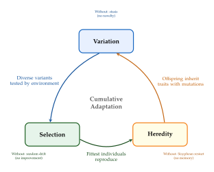
The three pillars of Darwinian evolution are deceptively simple:
Variation. Individuals in a population differ from one another. These differences arise from random mutations, recombination during sexual reproduction, and environmental perturbations. In computational terms, variation is the exploration mechanism that injects novelty into the search process.
Selection. Some variants are better suited to their environment than others. “Better suited” means, in the most stripped-down formulation, that they leave more copies of themselves in the next generation. Selection is the exploitation mechanism that retains and amplifies successful designs.
Heredity. Offspring resemble their parents. The traits that made a parent successful are transmitted – with some fidelity, but not perfectly – to the next generation. Heredity is the memory mechanism that allows the population to accumulate adaptations over time.
What makes this triad so powerful is not any single component but their interaction. Variation without selection is random drift. Selection without variation is stasis. Both without heredity are Sisyphean: each generation starts from scratch. Only when all three operate together does the ratchet of cumulative adaptation engage, and complexity begins its inexorable ascent.
Definition 1 (Evolutionary System).
An evolutionary system is a tuple where:
is a genotype space – the set of all possible encodings of individuals;
is a population of individuals at any given time;
is a variation operator that maps each genotype to a distribution over neighbouring genotypes (mutation, recombination);
is a selection operator that maps a population to a distribution over populations of the same or different size;
is a heritability function measuring the probability that a trait present in a parent is also present in an offspring.
The system evolves by iterating: .
Remark 1.
The definition above is deliberately abstract. It encompasses not only biological evolution but also genetic algorithms, evolution strategies, cultural evolution, and even certain economic processes. The generality is the point: any system satisfying these axioms will exhibit adaptive behaviour.
The philosophical import of Definition 1 is profound. It tells us that design – in the sense of functional organisation adapted to a purpose – does not require a designer. It requires only an evolutionary system operating for sufficient time. This insight liberates the AI researcher from a deep constraint: the assumption that intelligence must be hand-crafted. If evolution can design brains, perhaps it can also design neural networks, loss functions, training algorithms, and even the search processes that discover these components.
Insight.
Evolution as Universal Acid. Evolution is the only known process that reliably produces open-ended increases in complexity without requiring external intelligence to guide it. Every other optimisation method – gradient descent, Bayesian optimisation, reinforcement learning – operates within a fixed search space and objective function specified by a human designer. Evolution can modify both.
The Fitness Landscape Metaphor
In 1932, the population geneticist Sewall Wright introduced one of the most influential metaphors in all of biology: the adaptive landscape [32]. Imagine a vast, multidimensional terrain where each point represents a possible genotype and the height at that point represents the organism's fitness. Evolution, in this picture, is a population of hill climbers navigating a rugged landscape, seeking peaks while avoiding the treacherous valleys between them.
The metaphor is more than poetic. It provides a geometric framework for reasoning about the difficulty of evolutionary search, the role of population size, and the tension between exploration and exploitation.
Definition 2 (Fitness Landscape).
A fitness landscape is a triple where:
is a genotype space equipped with a notion of neighbourhood (typically defined by single-point mutations);
maps each genotype to its set of neighbours;
is a fitness function assigning a real-valued fitness to each genotype.
A genotype is a local optimum if for all . It is the global optimum if for all .
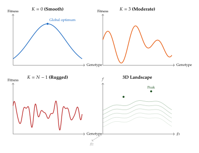
The crucial question for any evolutionary search is: how rugged is the landscape? A smooth, single-peaked landscape is trivially navigable by hill climbing. A landscape with many peaks of similar height, separated by deep valleys, is a combinatorial nightmare. Stuart Kauffman's NK model provides a tuneable framework for studying this question [1].
Definition 3 (NK Fitness Landscape).
An NK fitness landscape is defined over binary strings of length , . Each locus has a fitness contribution that depends on its own allele and the alleles at other specified loci (its epistatic partners). The total fitness is: (NK Fitness) where each is drawn independently and uniformly at random, and are the epistatic partners of locus .
The parameter controls the ruggedness of the landscape. When , there is no epistasis: each locus contributes independently to fitness, and the landscape has a single peak reachable by greedy hill climbing. When , every locus interacts with every other, the fitness function is essentially random, and the landscape is maximally rugged.
Proposition 1 (NK Landscape Ruggedness).
In an NK fitness landscape with loci and epistasis parameter :
The expected number of local optima grows exponentially with : for large .
When , there is exactly one local optimum, which is also the global optimum.
When , the expected number of local optima is .
The correlation between the fitness of neighbouring genotypes decreases monotonically with .
Proof.
For part (2), when the fitness function is separable: . Each locus can be optimised independently, yielding a unique global optimum.
For part (3), when , each depends on all bits, so the fitness values are i.i.d. uniform on . A genotype is a local optimum if for all Hamming-distance-1 neighbours . For random fitness values, the probability that a given genotype has the highest fitness among itself and its neighbours is . Since there are genotypes, the expected number of local optima is .
Parts (1) and (4) follow from the theory of random fields on hypercubes; see Kauffman [1] for the complete analysis.
The NK model teaches a lesson that resonates throughout this chapter: the difficulty of an optimisation problem depends not only on the size of the search space but on the structure of interactions between components. When components are tightly coupled (high ), the landscape becomes a fractal wilderness of competing peaks. When they are modular (low ), the landscape is smooth and navigable. This observation will reappear when we study neuroevolution in Neuroevolution, where modular network architectures are easier to evolve than monolithic ones.
Why Evolution Matters for AI
Why should a practitioner of deep learning, armed with automatic differentiation and GPU clusters, care about evolution? The answer lies in the fundamental limitations of gradient-based optimisation and the unique capabilities that evolutionary methods bring to the table.
The tyranny of differentiability.
Gradient descent, for all its triumphs, is shackled by a non-negotiable requirement: the objective function must be differentiable with respect to the parameters. This requirement is so deeply embedded in modern deep learning practice that we rarely pause to consider how constraining it is. It forces us to use smooth activation functions (or piecewise-linear approximations with well-defined subgradients), differentiable loss functions, and continuous parameter spaces. It prevents us from optimising over discrete choices: which layers to include, how to connect them, what data augmentation to apply, which loss function to use. Evolution faces no such constraint. An evolutionary algorithm can optimise over any space – discrete, continuous, mixed, structured, or unstructured – as long as candidate solutions can be evaluated.
The prison of fixed architecture.
When we train a neural network with gradient descent, we optimise the weights within a fixed computational graph. The architecture – the number of layers, their widths, connectivity patterns, activation functions – is frozen before training begins. This is akin to asking an engineer to optimise the fuel mixture of an engine without being allowed to modify the engine's design. Evolution operates at a higher level of abstraction: it can modify the architecture itself, adding or removing components, changing their connectivity, and even inventing entirely new computational primitives. This is the domain of neuroevolution, which we explore in Neuroevolution, and it connects directly to the neural architecture search methods discussed in 30.
The trap of local optima and mode collapse.
A single gradient-following trajectory is inherently local: it can only reach the nearest basin of attraction. Populations of diverse solutions, evolving in parallel, explore multiple basins simultaneously. Moreover, the population itself acts as a form of implicit memory, preserving diverse strategies that may become useful as the environment changes. This population-level diversity is the evolutionary antidote to the mode collapse that plagues generative adversarial networks and other generative models.
Evolution as meta-learning.
Perhaps the most profound reason to study evolutionary approaches is that evolution does not merely optimise a solution within a fixed framework – it optimises the framework itself. Biological evolution did not simply find good neural network weights for the brains of organisms; it invented the brain. It invented learning algorithms (synaptic plasticity), memory systems (the hippocampus), attention mechanisms (the superior colliculus), and generative models (the predictive processing hierarchy of the neocortex). In the language of machine learning, evolution is the ultimate meta-learner: it learns the learning algorithm.
Key Idea.
Evolution is the Only Known Source of Open-Ended Complexity. Among all known optimisation and search processes, biological evolution is the only one that has demonstrably produced an open-ended, unbounded increase in the complexity and diversity of its outputs over time. Every engineered optimisation method – gradient descent, simulated annealing, Bayesian optimisation, reinforcement learning – converges to a fixed point or limit cycle. Evolution, over 3.8 billion years, has produced an accelerating cascade of innovations: from prokaryotes to eukaryotes, from single cells to multicellular organisms, from simple nervous systems to the human brain. Understanding why evolution achieves this, and how to replicate it computationally, is one of the grand challenges of artificial intelligence.
Historical Note.
From Cybernetics to Evolutionary Computation. The idea of using evolution as a computational tool has roots as deep as computer science itself. In 1948, Alan Turing wrote a remarkable paper proposing “genetical or evolutionary search” as a method for machine intelligence, noting that it might be “more expedient” to evolve intelligent machines than to program them by hand. In the 1960s and 1970s, three independent traditions emerged:
Evolutionary programming (Fogel, Owens, and Walsh, 1966) in the United States, which evolved finite state machines;
Evolution strategies (Rechenberg, 1973; Schwefel, 1977) in Germany, which optimised real-valued engineering parameters [2][3];
Genetic algorithms (Holland, 1975) in the United States, which studied adaptation in abstract binary string spaces [4].
These traditions developed largely in isolation for two decades before converging in the 1990s under the umbrella term evolutionary computation. The subsequent explosion of work on genetic programming [5], neuroevolution [6], and evolutionary approaches to deep learning has made evolutionary methods an indispensable part of the modern AI toolkit.
Exercise 1.
Consider an NK fitness landscape with and .
How many possible genotypes exist?
Each fitness contribution depends on bits. How many entries does the lookup table for each contain?
Implement a random adaptive walk: start from a random genotype, examine all single-bit neighbours, move to the fittest neighbour if it improves fitness, and halt when no improving neighbour exists. Run 1000 walks and plot the distribution of local optima fitness values. How does this distribution change as increases from to ?
Exercise 2.
Identify the components of Definition 1 in each of the following systems:
A population of bacteria evolving antibiotic resistance;
A genetic algorithm optimising the weights of a small neural network;
The scientific community, where “genotypes” are theories and “fitness” is predictive accuracy.
For each system, discuss which component (variation, selection, or heredity) is the primary bottleneck limiting adaptive improvement.
Biological Foundations
Before we can build evolutionary algorithms that match the creative power of nature, we must understand the biological principles that make natural evolution so extraordinarily effective. This section is not a biology textbook – it is a targeted extraction of the ideas from evolutionary biology that have the deepest implications for algorithm design. We shall encounter Fisher's fundamental theorem, which reveals the mathematical engine driving adaptation; the Red Queen hypothesis, which explains why coevolution prevents complacency; punctuated equilibrium, which suggests that the most important evolutionary events are rare and sudden; and the Baldwin effect, which bridges the chasm between learning and evolution.
Each of these biological insights will become, in later sections, the foundation of a computational method.
Natural Selection: The Algorithm That Programs Itself
Let us state natural selection as an algorithm in the most explicit possible terms, stripping away the biological particulars to reveal the bare computational skeleton.
Algorithm 1: Natural Selection (Abstract Formulation).
[t]
- Input: Population in genotype space
- Input: Fitness function
- Input: Variation operator , selection operator
- Input: Number of generations
- for
- Evaluate: Compute for each
- Select: Choose parents Fitness-proportional or tournament
- Vary: Generate offspring Mutation + recombination
- Replace: Form new population from offspring (and possibly parents)
- return Best individual
The simplicity of alg:evo:natural_selection belies its power. Notice that the algorithm says nothing about the structure of the genotype space, the form of the fitness function, or the nature of the variation operator. It is, in the most precise sense, a black-box optimiser: it requires only the ability to evaluate fitness and to generate perturbed copies of existing solutions. This universality is both evolution's greatest strength and, as we shall see, its greatest weakness (it can be slow precisely because it uses so little information about the problem structure).
The mathematical heart of natural selection was formalised by R. A. Fisher in 1930, in what he grandly called the “fundamental theorem of natural selection” [33].
Definition 4 (Fitness and Selection Pressure).
Let be a population with fitness values . The mean fitness of the population is: (MEAN Fitness) The fitness variance is: (Fitness VAR) The selection pressure is the ratio , measuring the relative spread of fitness values.
Definition 5 (Heritability).
The heritability of a trait is the fraction of the total phenotypic variance that is attributable to genetic (heritable) variance: (Heritability) A trait with is perfectly heritable; a trait with is entirely determined by environmental noise and cannot respond to selection.
Theorem 1 (Fisher's Fundamental Theorem of Natural Selection).
Under the assumptions of random mating, constant environment, no mutation, no genetic drift, and additive genetic effects, the rate of increase of the mean fitness of a population equals the additive genetic variance in fitness: (Fisher) where is the additive genetic variance in fitness. Since variance is non-negative, mean fitness can never decrease under pure natural selection.
Proof.
Consider a population with discrete, non-overlapping generations. Let be the frequency of genotype with fitness . The mean fitness is . Under fitness-proportional selection (the infinite-population limit), the frequency of genotype in the next generation is . The new mean fitness is: The change in mean fitness is: In the continuous-time limit with additive genetic effects, is replaced by , the additive genetic variance, yielding (Fisher).
Fisher's theorem has a beautiful interpretation: natural selection is a variance-consuming engine. It converts genetic diversity (variance in fitness) into adaptive improvement (increase in mean fitness). When variance is high, adaptation is rapid. When variance is exhausted – when all individuals are equally fit – evolution grinds to a halt. This has immediate algorithmic implications: to maintain the adaptive power of an evolutionary algorithm, one must maintain population diversity, a principle known as diversity maintenance that recurs throughout this chapter.
Remark 2.
Fisher considered his theorem to be the biological analogue of the second law of thermodynamics: a one-directional arrow of change. Just as entropy never decreases, mean fitness never decreases under pure selection. The analogy is deeper than Fisher may have realised: both processes are driven by a variance or spread in the relevant quantity (microstates for thermodynamics, fitness values for evolution), and both halt at equilibrium when that variance vanishes.
Corollary 1.
If a population reaches a state where (all individuals have identical fitness), natural selection alone cannot produce further adaptation. Mutation or other sources of variation are required to restart the evolutionary process.
The Red Queen Hypothesis
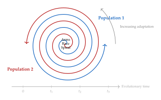
In Lewis Carroll's Through the Looking-Glass, the Red Queen tells Alice: “Now, here, you see, it takes all the running you can do, to keep in the same place.” In 1973, the evolutionary biologist Leigh Van Valen transformed this literary image into one of the most important hypotheses in evolutionary biology [34]: organisms must constantly adapt and evolve not merely to gain in fitness but simply to maintain their current fitness relative to the organisms they are co-evolving with.
The intuition is vivid. Consider the cheetah and the gazelle. As cheetahs evolve greater speed, the slower gazelles are eliminated, leaving only the fastest. But now the baseline has shifted: the average gazelle is faster, so only the fastest cheetahs can catch prey. Selection pressure on the cheetah intensifies, driving further speed increases. Both species run faster and faster, yet neither gains a lasting advantage. They are, in Carroll's phrase, running as fast as they can just to stay in the same place.
This dynamic is not limited to predator-prey relationships. It appears in host-parasite interactions (the vertebrate immune system is locked in a perpetual arms race with rapidly mutating pathogens), in sexual selection (the peacock's tail grows ever more elaborate because peahens evolve ever more discriminating preferences), and in competition between members of the same species for territory, mates, and resources.
Definition 6 (Red Queen Dynamics).
A system of co-evolving populations exhibits Red Queen dynamics if the fitness function of each population depends on the current state of at least one other population: (RED Queen) where denotes all populations except . The fitness landscape of each population is therefore non-stationary: it shifts as the other populations evolve.
Red Queen dynamics have a profound consequence: they prevent convergence to any fixed point. In a system with Red Queen dynamics, the very concept of an “optimum” becomes time-dependent. The best strategy at time may be mediocre at time because the opponents have adapted.
Proposition 2 (Red Queen Prevents Fixed-Point Convergence).
Consider a two-population coevolutionary system with fitness functions and satisfying the strictly competitive condition: (a zero-sum or constant-sum game). If the joint strategy space admits no pure Nash equilibrium, then any evolutionary dynamics on this system exhibits persistent cycling: no fixed point is asymptotically stable.
Proof.
Suppose for contradiction that is asymptotically stable. Then it must be a Nash equilibrium: for all , and similarly for player 2. But by assumption, no pure Nash equilibrium exists, yielding a contradiction.
More precisely, for continuous dynamics (such as replicator dynamics), the non-existence of pure equilibria implies that any interior rest point is a centre or a saddle, not an attractor. The resulting trajectories are cycles or quasi-periodic orbits in the joint strategy space.
The Red Queen hypothesis provides the biological motivation for coevolutionary algorithms, which we shall study extensively in later sections. In generative modelling, the most famous example of Red Queen dynamics is the GAN: the generator and discriminator are locked in exactly the kind of coevolutionary arms race that Van Valen described, each constantly adapting to the other's improvements.
Example 1 (GANs as Red Queen Systems).
In a generative adversarial network, the generator and discriminator play a minimax game: This is precisely a constant-sum coevolutionary game. As the generator improves, the discriminator must adapt to distinguish ever-more-realistic fakes. As the discriminator improves, the generator must produce ever-more-realistic outputs. The training dynamics often exhibit the cycling behaviour predicted by Proposition 2, manifesting as training instability and mode cycling.
Exercise 3.
Consider the Rock-Paper-Scissors game as a two-player coevolutionary system.
Write down the payoff matrices and for the two players.
Show that there is no pure Nash equilibrium.
Simulate replicator dynamics: for player 1, and similarly for player 2, where and are mixed strategies. Verify that the trajectories cycle around the mixed Nash equilibrium .
Punctuated Equilibrium and Neutral Networks
The fossil record tells a story that Darwin himself found troubling: species do not change gradually and continuously as his theory seemed to predict. Instead, they persist for millions of years in a state of near-stasis, then undergo rapid bursts of morphological change. In 1972, Niles Eldredge and Stephen Jay Gould formalised this observation as the theory of punctuated equilibrium [35]: the history of life is not a smooth ramp but a staircase, with long flat treads separated by abrupt risers.
Why would evolution exhibit such stop-and-start dynamics? One explanation comes from the structure of fitness landscapes. If the landscape contains neutral networks – connected sets of genotypes with equal fitness – then a population can wander along these neutral networks without any change in phenotype or fitness. The population is exploring, but from the outside, it appears to be standing still. Then, suddenly, the neutral walk reaches a region of genotype space adjacent to a higher-fitness peak, and the population rapidly climbs to the new peak. The result is exactly the punctuated pattern: long periods of apparent stasis (neutral drift along the plateau) interrupted by bursts of rapid change (climbing a newly accessible peak).
Definition 7 (Neutral Network).
Given a fitness landscape and a fitness value , the neutral network at fitness is the graph where: A neutral network is extensive if grows exponentially with the dimension of the genotype space.
Motoo Kimura's neutral theory of molecular evolution [36] provides the theoretical foundation: most mutations at the molecular level are selectively neutral, neither beneficial nor deleterious. These neutral mutations accumulate through random genetic drift rather than natural selection. The population performs a random walk on the neutral network, and this walk is invisible to selection.
Proposition 3 (Neutral Networks Facilitate Escape from Local Optima).
Consider a fitness landscape with a local optimum at fitness and a global optimum at fitness . Suppose the neutral network is extensive and connected, and that some genotype has a neighbour with (a “portal” to a higher peak). Then a population performing neutral drift on will, with probability 1, eventually reach and discover the portal , escaping the local optimum without ever decreasing fitness.
Proof.
On a finite, connected graph, a random walk visits every node with probability 1 (this is a consequence of the recurrence of random walks on finite graphs). Since is connected and , the neutral random walk will eventually reach . At that point, the mutation operator has a non-zero probability of producing , and since , selection will favour and initiate a climb toward the higher peak.
This result has a striking computational implication: neutral networks transform local optima from traps into way-stations. A population that would be forever stuck at a local optimum under pure hill climbing can escape via neutral drift, provided the fitness landscape contains sufficient neutral structure.
Remark 3 (Connection to Flat Minima in Deep Learning).
The concept of neutral networks resonates with the observation in deep learning that “flat” minima – regions of parameter space where the loss function is approximately constant – tend to generalise better than “sharp” minima. In evolutionary terms, flat minima are neutral networks in weight space. The stochastic gradient descent (SGD) noise performs a function analogous to neutral drift, exploring the flat region and implicitly selecting for broader, more robust minima. This connection between evolutionary neutral theory and deep learning generalisation deserves further investigation.
Exercise 4.
Consider the binary genotype space with a fitness function that counts the number of “blocks” of four consecutive identical bits (e.g., 1111 or 0000). Two genotypes that have the same number of blocks have identical fitness, creating neutral networks.
How many distinct fitness levels are possible?
Implement a neutral random walk: at each step, flip a random bit, accept the move if fitness does not decrease. Track the fraction of moves that are neutral versus improving.
Starting from the all-zeros string (which has high fitness), measure the number of neutral steps before reaching a genotype with maximum fitness. How does this scale with the number of bits?
The Baldwin Effect: Learning Guides Evolution
In 1896, the psychologist James Mark Baldwin proposed a mechanism by which learning – a lifetime phenomenon – could influence evolution – a generational phenomenon – without invoking the discredited Lamarckian inheritance of acquired characteristics. The idea, now known as the Baldwin effect, runs as follows:
Imagine a population of organisms facing a novel environmental challenge. Some organisms have genotypes that make them more capable of learning the appropriate response, even if they do not innately possess it. These fast-learning organisms survive and reproduce more effectively than slow-learning ones. Over generations, selection favours genotypes that facilitate learning. Eventually, what was originally learned behaviour may become partially or fully innate through a process called genetic assimilation: the costly and time-consuming learning is replaced by hardwired neural circuitry.
The Baldwin effect has a precise mathematical formulation in terms of fitness landscapes. Recall that an organism's fitness depends on its phenotype (behaviour, morphology), which is determined by both genotype and lifetime experience (learning). An organism that can learn effectively has a broader basin of attraction in genotype space: even if its genotype is not perfectly adapted, learning can compensate and pull the phenotype toward a high-fitness region.
Proposition 4 (Baldwin Effect: Learning Smooths the Fitness Landscape).
Let be the “innate” fitness landscape (fitness without learning) and let represent the fitness gain from lifetime learning. If the effective fitness is: (Baldwin) and the learning gain is a smoothing function that is larger for genotypes near (but not at) fitness peaks, then is smoother than . Specifically, if is inversely proportional to in a continuous genotype space, the effective landscape has fewer local optima than .
Proof sketch.
Local optima of at which receive maximal learning boost , potentially merging with nearby optima. Genotypes on steep fitness gradients receive minimal learning boost. The net effect is to “fill in” valleys between peaks: a genotype in a valley can learn its way to a nearby peak, receiving a fitness boost that raises its effective fitness above the valley floor. The mathematical details depend on the specific forms of and , but the qualitative effect – landscape smoothing – is robust across a wide range of assumptions. See Hinton and Nowlan (1987) for the seminal computational demonstration.
The Baldwin effect has deep implications for the relationship between evolution and learning in AI systems. It suggests that the most effective strategy is not to evolve complete solutions but to evolve learning algorithms – organisms (or neural networks) that can rapidly adapt to their environment during their lifetime. This is precisely the philosophy behind meta-learning approaches, and it connects directly to the neural architecture search methods discussed in 30, where the “genotype” is the network architecture and “learning” is gradient-based training of the weights.
Key Idea.
The Baldwin Bridge. The Baldwin effect bridges evolution and learning:
Evolution discovers architectures that are amenable to learning.
Learning discovers parameters within those architectures that solve the current task.
Over generations, evolutionary pressure internalises the most useful learned behaviours into the architecture itself.
This three-step process is the biological template for modern neuroevolution and neural architecture search, where evolution operates on the slow timescale of architecture design and gradient descent operates on the fast timescale of weight optimisation.
Example 2 (Baldwin Effect in Neuroevolution).
Consider evolving neural network architectures for image classification. The genotype encodes the architecture (layer types, connectivity, hyperparameters); the phenotype is the trained network. During evaluation, each candidate architecture is trained by gradient descent for a fixed number of epochs. Architectures that are easier to train – that reach higher accuracy in fewer epochs – receive higher evolutionary fitness. Over generations, evolution selects for architectures with favourable loss landscapes: those with broad basins of attraction, smooth gradients, and good initialisation properties. The Baldwin effect is at work: learning (gradient descent) smooths the fitness landscape over architectures, guiding evolution toward designs that are inherently amenable to optimisation.
Exercise 5.
Replicate the classic Hinton–Nowlan (1987) experiment:
Create a binary genotype of length with a single target string (all ones) as the fitness peak.
Each allele can be 0, 1, or “?” (plastic, learnable). During lifetime, the “?” alleles randomly take values 0 or 1 each trial, for up to trials.
Fitness = number of remaining trials when the target is first matched (0 if never matched).
Run the evolutionary simulation for 200 generations with a population of 1000. Plot the fraction of fixed (non-plastic) correct alleles over time.
Discuss: why does the number of “?” alleles decrease over generations? How does this illustrate genetic assimilation?
Classical Evolutionary Algorithms
With the biological foundations in place, we now turn to the computational incarnations of evolutionary principles. The history of evolutionary computation is a story of convergent invention: three independent research traditions, on three continents, each abstracted the essential logic of Darwinian evolution into computational form. John Holland's genetic algorithms in Michigan, Ingo Rechenberg and Hans-Paul Schwefel's evolution strategies in Berlin, and Lawrence Fogel's evolutionary programming in San Diego all emerged in the 1960s and 1970s, each capturing different facets of the evolutionary process. A fourth tradition, John Koza's genetic programming, extended evolutionary search to the space of computer programs in the early 1990s. And in 2002, Kenneth Stanley and Risto Miikkulainen introduced NEAT, demonstrating that evolution could construct neural network topologies from scratch.
This section provides rigorous treatments of each approach, emphasising the mathematical principles that make them work (and the conditions under which they fail).
Genetic Algorithms
Holland's genetic algorithms (GAs) are the oldest and most widely known family of evolutionary methods [4][37]. The original formulation operates on fixed-length binary strings, a deliberate abstraction that separates the study of evolutionary dynamics from the specifics of any particular application domain.
Definition 8 (Genetic Algorithm).
A genetic algorithm operates on a population of binary strings of length . Each generation proceeds in four steps:
Fitness evaluation: Compute for all .
Selection: Choose parents from with probability proportional to fitness (fitness-proportional selection, also called roulette wheel selection): (Roulette)
Crossover: With probability , pair parents and exchange genetic material via one-point crossover: choose a random position and create offspring by swapping the segments after position .
Mutation: Flip each bit independently with probability (typically ).
Algorithm 2: Simple Genetic Algorithm.
[t]
- Input: Population size , string length , crossover rate , mutation rate , generations
- Initialise random binary strings from
- for
- Evaluate fitness for all
- for
- Select parents via roulette wheel ((Roulette))
- if
- Choose crossover point
- else
- ,;
- for
- Flip bit with probability
- return
Holland's most celebrated theoretical contribution is the schema theorem, which attempts to explain why genetic algorithms work by analysing the dynamics of schemata – templates that match subsets of the search space.
Definition 9 (Schema).
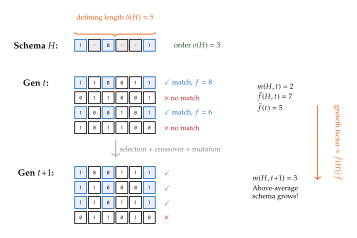
A schema is a template where is a wildcard matching either 0 or 1. The order of a schema is the number of non-wildcard positions. The defining length is the distance between the first and last non-wildcard positions. A genotype is an instance of schema , written , if for all positions where .
Theorem 2 (Holland's Schema Theorem).
Let be the number of instances of schema in the population at generation . Under fitness-proportional selection, one-point crossover with rate , and bit-flip mutation with rate , the expected number of instances in the next generation satisfies: (Schema) where is the average fitness of instances of at time , and is the population average fitness.
Proof.
Under fitness-proportional selection, the expected number of copies of schema selected is , since each instance is selected with probability proportional to its fitness.
One-point crossover at position destroys schema only if falls within the defining length of . The probability of this is at most , so crossover preserves with probability at least .
Each of the defining positions must survive mutation (probability per position), giving survival probability .
Multiplying these three factors yields the bound in (Schema).
The schema theorem has an appealing interpretation: short, low-order, above-average schemata receive exponentially increasing numbers of instances. Holland called this the implicit parallelism of genetic algorithms: while explicitly evaluating individuals per generation, the GA implicitly processes schemata.
Caution.
Limitations of the Schema Theorem. The schema theorem, despite its elegance, has been extensively criticised:
It provides only a lower bound that can be extremely loose.
It analyses one-generation dynamics and does not guarantee long-term convergence.
The “implicit parallelism” argument assumes that schemata are approximately independent, which is false in general due to hitchhiking and epistasis.
It does not account for the constructive effects of crossover (creating new, beneficial combinations), only its destructive effects.
Alternative selection methods (tournament, ranking) are not covered by the analysis.
Modern GA theory relies on runtime analysis, Markov chain models, and computational complexity arguments rather than schema-theoretic reasoning.
Exercise 6.
The OneMax problem has fitness (count the number of ones).
Implement the simple GA (alg:evo:sga) and run it on OneMax with , , , .
Plot the best and mean fitness over 200 generations.
Compare with a evolutionary algorithm (single individual, bit-flip mutation only, no crossover, accept if fitness does not decrease). Which converges faster?
Explain your observations in terms of the schema theorem. What schemata are the “building blocks” of OneMax?
Evolution Strategies
While Holland's genetic algorithms were designed for discrete optimisation, Ingo Rechenberg and Hans-Paul Schwefel independently developed evolution strategies (ES) for continuous optimisation – the problem of finding for a (possibly non-differentiable, noisy, or multimodal) objective function [2][3].
The key insight of evolution strategies is that the mutation operator should be self-adaptive: the algorithm does not merely evolve candidate solutions but also evolves the parameters of its own variation operator. This is a remarkable instance of the meta-learning principle we discussed in Why Evolution Matters for AI: evolution learning how to evolve.
Definition 10 (Evolution Strategy).
An evolution strategy operates on individuals where is the solution vector and is the vector of mutation step sizes. Two selection variants are standard:
-ES: Generate offspring from parents (). Select the best offspring as parents for the next generation. Parents do not survive.
-ES: Generate offspring and select the best from the combined pool of parents and offspring. Parents can survive (elitist).
Offspring are generated by: (ES Sigma) where and are the learning rates for self-adaptation.
The mutation step sizes evolve alongside the solution . If a particular step size is too large (causing offspring to overshoot good regions) or too small (causing stagnation), selection will favour individuals with better-tuned step sizes. Over generations, the step sizes adapt to the local curvature of the fitness landscape – large steps in flat directions, small steps in steep directions.
This self-adaptation of step sizes was a revolutionary concept when Rechenberg introduced it in 1973. It anticipated by decades the adaptive learning rate methods (Adam, AdaGrad, RMSProp) that are now standard in deep learning. The principle is the same: each parameter should be updated with a step size matched to the local geometry of the loss surface.
CMA-ES: The gold standard.
The Covariance Matrix Adaptation Evolution Strategy (CMA-ES), developed by Hansen and Ostermeier [38], represents the state of the art in derivative-free continuous optimisation. While the basic ES adapts individual step sizes per dimension (a diagonal covariance matrix), CMA-ES adapts the full covariance matrix of the mutation distribution, capturing correlations between variables.
Definition 11 (CMA-ES).
The CMA-ES maintains a search distribution where:
is the mean of the distribution (current best estimate);
is the global step size;
is the covariance matrix (positive definite, symmetric).
At each generation:
Sample: Generate offspring: , where , .
Rank: Sort offspring by fitness: .
Update mean: (CMA MEAN) where are recombination weights summing to 1, and .
Update evolution path: (CMA PATH) where is the learning rate and is the effective number of parents.
Update covariance matrix: (CMA COV) where and are learning rates.
Update step size: via cumulative step-size adaptation (CSA) using an evolution path .
Algorithm 3: CMA-ES (Covariance Matrix Adaptation Evolution Strategy).
[t]
- Input: Objective (to minimise), initial mean , initial
- Initialise ,; ,;
- Set ,;
- Set weights for
- Set
- Set ,;
- Set ,;
- for until convergence
- for
- Sort:
- Weighted mean of best
- Update via (CMA COV)
- return
The beauty of CMA-ES lies in its ability to learn the local geometry of the fitness landscape from the distribution of successful mutations. The covariance matrix captures the shape of the fitness function's level sets near the current mean: its eigenvectors align with the principal axes of the local quadratic approximation, and its eigenvalues reflect the relative scales along these axes. The evolution path provides temporal coherence, encouraging the covariance matrix to adapt in directions of consistent progress.
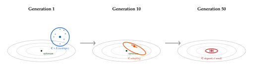
Remark 4 (CMA-ES and Natural Gradient).
There is a deep connection between CMA-ES and the natural gradient method from information geometry. The CMA-ES mean update ((CMA MEAN)) can be interpreted as a natural gradient step on the fitness function, using the Fisher information metric of the Gaussian search distribution as the Riemannian metric. Specifically, the natural gradient of the expected fitness with respect to is: (Natural GRAD) The CMA-ES update approximates this using the best samples (a form of truncation selection) rather than all samples. This connection explains why CMA-ES is invariant to affine transformations of the search space – a property shared by natural gradient methods but not by vanilla gradient descent.
Exercise 7.
Implement CMA-ES and test it on the Rosenbrock function:
Run CMA-ES with , starting from , .
Plot the evolution of and the eigenvalues of over generations. How do they reflect the “banana-shaped” valley of the Rosenbrock function?
Compare the number of function evaluations to reach against random search and a -ES with isotropic mutation.
Exercise 8.
Compare -ES and -ES on the following multimodal function in dimensions:
Which selection scheme is more robust to local optima? Why?
How does the population size affect the trade-off between exploration and exploitation?
Genetic Programming
Genetic algorithms evolve strings. Evolution strategies evolve vectors. But the true prize of evolutionary computation has always been more ambitious: can we evolve programs? John Koza's genetic programming (GP) answers in the affirmative [5]. In GP, the genotype is not a fixed-length string but a variable-size tree representing a computer program. The leaves of the tree are terminals (constants, variables, sensor inputs), and the internal nodes are functions (arithmetic operators, conditional statements, domain-specific operations). Evolution operates by composing, decomposing, and recombining these trees, searching through the space of all expressible programs for one that solves the task.
Definition 12 (Genetic Programming).
A genetic programming system is defined by:
A function set of internal node operators, each with a specified arity (e.g., has arity 2, has arity 1);
A terminal set of leaf node values (variables, constants);
A fitness function that evaluates program quality (typically prediction error on training data);
Closure: every function in must accept as input any value that can be produced by any function or terminal (ensures all random trees are valid);
Sufficiency: must be expressive enough to represent a solution.
The search space is the set of all trees that can be constructed from and .
The variation operators in GP are designed for tree structures:
Crossover (subtree swap).
Select two parent trees. In each parent, choose a random subtree. Swap the subtrees between parents. The resulting offspring inherit structure from both parents – a form of compositional recombination that has no analogue in fixed-length string representations.
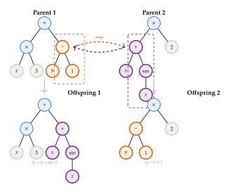
Mutation (subtree replacement).
Select a random node in the tree. Replace the subtree rooted at that node with a randomly generated subtree. This introduces genuinely new structure that may not have existed in the population.
The bloat problem.
GP trees tend to grow in size over generations even when the extra nodes contribute nothing to fitness – a phenomenon known as bloat or code growth. Bloat occurs because larger trees have more crossover points, making them more likely to survive crossover intact (the “defence against crossover” hypothesis). Unchecked bloat leads to enormous, uninterpretable trees that waste computational resources.
The standard countermeasure is parsimony pressure: adding a penalty for tree size to the fitness function: (Parsimony) where is the number of nodes and is a parsimony coefficient. Lexicographic parsimony pressure, which prefers smaller trees only among individuals of equal fitness, is often more effective than the additive penalty.
Historical Note.
Koza's Human-Competitive Results. Between 1992 and 2010, Koza and collaborators demonstrated that GP could automatically rediscover or exceed human-designed solutions in domains including:
Electronic circuit design: GP evolved analogue circuits (filters, amplifiers) that matched or exceeded the performance of circuits patented by human engineers.
Controller design: GP evolved control laws for complex dynamical systems that outperformed hand-tuned PID controllers.
Symbolic regression: GP rediscovered known physical laws (Kepler's third law, Ohm's law) from raw data without being told the functional form to search for.
These results established the principle that evolutionary search can be creative: it can discover solutions that a human designer would not have considered, by exploring regions of program space far from conventional designs.
Exercise 9.
Implement a simple GP system for symbolic regression:
Function set: where if , else .
Terminal set: .
Generate 100 data points from with .
Fitness = negative mean squared error on training data.
Run GP with population 500, tournament selection (size 7), subtree crossover (rate 0.9), subtree mutation (rate 0.1), maximum tree depth 10, for 100 generations.
Does GP rediscover the true function? How does parsimony pressure affect the result?
Neuroevolution
The holy grail of evolutionary approaches to AI is neuroevolution: the evolution of neural network architectures and/or weights. If neural networks are the most powerful function approximators known, and if evolution is the most creative search process known, then combining the two should yield something extraordinary. This intuition has been validated repeatedly, from the early work of Yao (1999) to the modern successes of large-scale neuroevolution at OpenAI [9] and Uber [10].
The landmark contribution in this field is Kenneth Stanley and Risto Miikkulainen's NeuroEvolution of Augmenting Topologies (NEAT) [6], which solved three fundamental problems that had plagued earlier neuroevolution approaches:
The competing conventions problem: Two networks may encode the same function with different topologies. If crossover naively combines them, the offspring may inherit redundant structure and perform poorly.
The protection of innovation problem: When a structural mutation adds a new node or connection, the new structure initially performs poorly (the weights are random). Without protection, selection immediately eliminates these innovations before they have time to be optimised.
The minimal complexity problem: How should networks be initialised? Starting with large, randomly connected networks wastes search effort on unnecessary structure.
NEAT addresses all three problems with elegant mechanisms: innovation numbers for structural alignment, speciation for innovation protection, and complexification starting from minimal networks.
Definition 13 (NEAT Encoding).
A NEAT genome encodes a neural network as two lists:
Node genes: each specifying a node ID and type (input, hidden, or output);
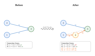
Connection genes: each specifying an input node, output node, weight , enabled/disabled flag, and a globally unique innovation number.
The innovation number is assigned sequentially when a new structural mutation first appears anywhere in the population. If the same structural mutation occurs independently in two individuals, it receives the same innovation number (tracked via a global innovation database). Innovation numbers provide a natural alignment for crossover: matching genes (same innovation number) are inherited from one parent or the other; disjoint and excess genes (present in one parent but not the other) indicate structural differences.
Definition 14 (NEAT Crossover).
Given two parent genomes and with fitness :
Matching genes (same innovation number in both parents): inherited randomly from either parent.
Disjoint genes (innovation numbers within the range of the other parent but not present): inherited from the fitter parent .
Excess genes (innovation numbers beyond the range of the other parent): inherited from the fitter parent .
Mutation operators.
NEAT uses three types of mutation:
Weight mutation: Perturb existing connection weights by Gaussian noise or replace with a new random value.
Add connection: Add a new connection between two previously unconnected nodes, with a random initial weight and a new innovation number.
Add node: Split an existing connection by disabling it, inserting a new hidden node, and creating two new connections: one from the old input to the new node (weight 1) and one from the new node to the old output (weight equal to the old connection's weight). This ensures the mutation is initially neutral: the network's behaviour is unchanged.
Speciation.
To protect structural innovations, NEAT divides the population into species – groups of individuals with similar topologies. Individuals compete primarily within their species, not against the entire population. This gives newly evolved structures time to optimise their weights before facing competition from well-tuned networks with different topologies.
The distance between two genomes is: (NEAT Distance) where is the number of excess genes, is the number of disjoint genes, is the average weight difference across matching genes, , and are importance coefficients. Individuals are assigned to the species of the first representative whose distance is below a threshold .
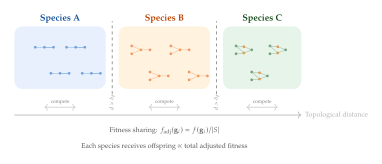
Fitness sharing ensures that each species receives a proportional share of the next generation's population. The adjusted fitness of individual in species is: (NEAT Sharing) where is the number of individuals in species . This prevents any single species from dominating the population, maintaining topological diversity.
Algorithm 4: NEAT (NeuroEvolution of Augmenting Topologies).
[t]
- Input: Population size , generations , compatibility threshold
- Initialise : minimal networks (inputs fully connected to outputs, no hidden nodes)
- Assign all individuals to one species
- for
- Evaluate fitness for all
- Speciate: For each , compute to each species representative; assign to first species with , or create new species
- Adjust fitness: for each individual in species
- Allocate offspring: Species produces offspring
- Reproduce within each species:
- for each species
- Keep champion of unchanged (elitism)
- Produce offspring via:
- Crossover of two parents (Definition 14) with probability
- Or asexual reproduction (clone + mutate)
- Apply mutations: weight perturbation, add connection, add node
- union of all offspring
- return Best individual across all generations
Proposition 5 (NEAT Complexification).
Starting from minimal networks (no hidden nodes), NEAT discovers increasingly complex topologies through structural mutations. This complexification principle ensures:
Search begins in the lowest-dimensional subspace of network topologies, minimising the initial search burden.
Structural additions are made only when they provide a fitness advantage, avoiding unnecessary complexity.
The trajectory through topology space follows a path of increasing dimensionality, analogous to the “continuation methods” used in numerical analysis to solve difficult nonlinear systems by starting from an easy problem and gradually increasing complexity.
Proof sketch.
The initial population consists of networks with zero hidden nodes. The only source of structural growth is the add-node and add-connection mutations. An add-node mutation increases the number of hidden nodes by one and the number of connections by two (minus one disabled). By (NEAT Sharing), fitness sharing within species prevents networks with more structure from monopolising the population unless their additional structure is beneficial. Therefore, structural growth is effectively gated by fitness improvement: complexity increases only when it pays.
The analogy to continuation methods is precise: in continuation methods, one solves starting from (easy problem) and gradually increasing to 1 (hard problem), using the solution at each stage as the starting point for the next. In NEAT, the “difficulty parameter” is network complexity, and the solution at each complexity level serves as the seed for the next.
HyperNEAT and indirect encodings.
A limitation of NEAT's direct encoding – where every connection is explicitly listed in the genome – is that genome size grows linearly with network size. For large networks, this makes evolution prohibitively slow. HyperNEAT (Stanley, D'Ambrosio, and Gauci, 2009) addresses this by evolving an indirect encoding: a Compositional Pattern Producing Network (CPPN) that takes as input the coordinates of a potential connection's source and target nodes and outputs the connection weight. The full network is constructed by querying the CPPN at every pair of node positions.
This indirect encoding has a profound advantage: it can exploit geometric regularities such as symmetry, repetition, and gradient patterns that are ubiquitous in biological neural networks and in the physical world. A CPPN with a sine activation can produce periodic connection patterns; one with Gaussian activations can produce locally connected receptive fields. The genome size is determined by the CPPN, which can be much smaller than the target network, enabling the evolution of networks with millions of connections from genomes with only hundreds of parameters.
Remark 5 (Connection to Neural Architecture Search).
NEAT and HyperNEAT are, in hindsight, early neural architecture search methods. The contemporary NAS literature, reviewed in 30, has largely replaced evolutionary search with gradient-based methods (DARTS) or reinforcement learning (Zoph and Le, 2017). However, evolutionary NAS remains competitive: Real et al. [7] showed that regularised evolutionary search matches or exceeds RL-based NAS on image classification benchmarks, while being simpler to implement and parallelise. The connection runs deeper: NEAT's innovation numbers anticipated the “one-shot” NAS idea of sharing a single supernetwork, and speciation anticipated the multi-objective approaches that balance accuracy against efficiency.
Exercise 10.
Implement NEAT and evolve a network to solve the XOR problem:
Start with a population of 150 minimal networks (2 inputs, 1 output, no hidden nodes, fully connected).
Fitness = , where the sum is over the four XOR input-output pairs.
Run for 300 generations. How many hidden nodes does the best solution typically require?
Visualise the best network's topology. Does NEAT find the minimal solution (one hidden node)?
Record the number of species over time. How does speciation affect the search dynamics?
Exercise 11.
Compare neuroevolution and backpropagation on a simple function approximation task: learn from 50 noisy samples.
Train a fixed-architecture MLP (2 hidden layers, 10 nodes each) with Adam for 1000 epochs.
Evolve network topologies with NEAT for the same computational budget (measure in total forward passes).
Compare: (a) test MSE, (b) network complexity (number of parameters), (c) generalisation to unseen values.
Under what conditions might neuroevolution outperform gradient-based training? Consider the role of architecture versus weight optimisation.
Conjecture 1 (Evolutionary Advantage in Sparse Reward Landscapes).
In reinforcement learning environments with sparse or deceptive reward signals, neuroevolution with novelty-based selection (see Why Evolution Matters for AI and later sections on novelty search [8]) will asymptotically outperform gradient-based policy optimisation methods. The conjecture rests on two observations:
Gradient-based methods require reward signal to flow back through the computational graph; in sparse-reward settings, the gradient is zero almost everywhere.
Evolution evaluates whole-episode returns and does not require temporal credit assignment, making it naturally suited to sparse rewards.
Partial evidence comes from Salimans et al. [9] and Such et al. [10], who showed that simple evolution strategies can match deep RL on Atari games, and from Lehman et al. [11], who demonstrated that large-scale evolutionary strategies can discover novel behaviours inaccessible to gradient methods.
Open Problem 1.
Open Problems in Neuroevolution. Several fundamental questions in neuroevolution remain unresolved:
Scalability: Can neuroevolution compete with gradient-based training for networks with billions of parameters? Current evidence suggests that evolution is most effective for architecture search (outer loop) while gradient descent handles weight optimisation (inner loop).
Indirect encodings: What is the optimal level of indirection? Direct encodings are flexible but unscalable; highly indirect encodings (like CPPNs) impose strong geometric priors that may not suit all tasks.
Lifetime learning: How should Baldwinian learning interact with evolution in neuroevolution systems? The optimal balance between innate structure (evolved) and learned structure (trained) is task-dependent and poorly understood.
Open-ended evolution: Can neuroevolution systems exhibit the open-ended complexity increase observed in biological evolution? This requires moving beyond fixed fitness functions to environments that co-evolve with the agents inhabiting them.
Example 3 (Evolving Atari Agents without Gradients).
Such et al. [10] demonstrated a striking result: a simple genetic algorithm with fixed-topology networks and Gaussian weight perturbation can solve several Atari 2600 games, matching or exceeding the performance of deep reinforcement learning methods such as DQN and A3C. The algorithm is remarkably simple:
Maintain a population of parameter vectors , where is the number of weights in a fixed convolutional network.
Evaluate each by running one episode of the Atari game and recording the total reward .
Select the top individuals (truncation selection).
Generate the next generation by adding Gaussian noise to copies of the elite individuals: , where selects a random elite and .
The key insight is that this algorithm is embarrassingly parallel: each fitness evaluation is independent, so 1000 evaluations can run simultaneously on 1000 CPU cores. On a cluster with 720 cores, the GA solved Frostbite in one hour – a task that required days of training for gradient-based RL methods. This result challenges the assumption that gradient-based optimisation is always superior and highlights the practical advantages of evolutionary methods in the age of massively parallel computing.
Example 4 (Evolution Strategies for Policy Search).
Salimans et al. [9] showed that evolution strategies can serve as a scalable alternative to reinforcement learning for continuous control tasks. Their approach uses the -ES framework with a twist: instead of explicitly maintaining a population, they represent each individual as a perturbation of a shared parameter vector: (ES Policy Update) where , is the episode return, is the noise standard deviation, and is the learning rate. This update rule is equivalent to estimating the gradient of expected return via finite differences in random directions – a zeroth-order gradient estimate.
The remarkable finding is that this simple approach achieves competitive performance with PPO and TRPO on MuJoCo locomotion tasks, while scaling linearly to thousands of parallel workers. With 1440 CPU cores, ES trained a humanoid walker in 10 minutes – a task requiring hours for gradient-based RL on a single GPU.
Exercise 12.
Show that the ES update in (ES Policy Update) is an unbiased estimate of the gradient of the smoothed objective:
Use the log-derivative trick: .
Show that when and the sampling distribution is reparameterised.
Discuss: as , . Why can't we simply set to be very small? What is the variance of the gradient estimate as a function of ?
Exercise 13.
Compare genetic algorithms and evolution strategies on the Rastrigin function:
Implement a GA with real-valued representation (using BLX- crossover) and tournament selection.
Implement a -ES with self-adaptive step sizes.
Implement CMA-ES.
Compare all three on . For each, report the number of function evaluations to reach . Which method scales best with dimensionality?
Insight.
The Exploration-Exploitation Spectrum of Evolutionary Methods. The classical evolutionary algorithms form a spectrum from high-exploration to high-exploitation:
Genetic algorithms with high mutation rates and large populations explore broadly but converge slowly;
Evolution strategies with self-adaptive step sizes balance exploration and exploitation through local curvature estimation;
CMA-ES combines aggressive exploitation (natural gradient steps toward the best solutions) with principled exploration (sampling from an adapted Gaussian that captures the landscape geometry).
The choice of algorithm should be guided by the structure of the problem: highly multimodal landscapes favour population-based exploration (GA, large-population ES), while unimodal or moderately multimodal landscapes favour the aggressive exploitation of CMA-ES. Neuroevolution methods like NEAT add a further dimension: they explore the space of architectures, not just parameters, opening possibilities that are invisible to all parameter-only methods.
Remark 6 (Evolution as Zeroth-Order Optimisation).
From the optimisation theory perspective, evolutionary algorithms belong to the family of zeroth-order (derivative-free) methods: they require only function values , not gradients or Hessians . Classical complexity theory tells us that zeroth-order methods require function evaluations per effective gradient step in dimensions, compared to for first-order methods. This suggests an inherent inefficiency – but the comparison is misleading for three reasons:
Zeroth-order methods can handle non-differentiable, stochastic, and discrete objectives where gradients do not exist.
Function evaluations can be trivially parallelised across thousands of workers, while gradient computation is often sequential through the computational graph.
Evolution can search over combinatorial spaces (architectures, programs, topologies) that are fundamentally inaccessible to gradient methods.
The practical lesson: use gradients when you can, evolution when you must, and the combination of both when you want the best of both worlds.
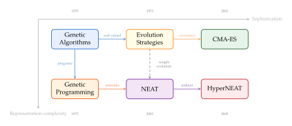
We have now surveyed the foundational methods of evolutionary computation, each capturing a different aspect of the Darwinian engine. Genetic algorithms taught us the power of recombination and the implicit parallelism of population-based search. Evolution strategies revealed the principle of self-adaptation and the deep connection to natural gradient methods. Genetic programming showed that evolution can search the space of programs, not merely the space of parameters. And neuroevolution – particularly NEAT – demonstrated that the architecture of intelligence itself can be an object of evolutionary discovery.
Yet these classical methods, for all their elegance, share a common limitation: they optimise toward a single, fixed fitness function specified by the human designer. In the next sections, we shall see what happens when we remove this constraint – when we allow fitness itself to evolve, when we replace optimisation with exploration, and when we seek not the single best solution but an entire archive of diverse, high-quality solutions. This is the frontier of evolutionary AI, and it brings us closer to the open-ended creativity of biological evolution than any fixed-objective method ever could.
Coevolutionary Algorithms
In every evolutionary algorithm we have encountered so far, fitness has been a fixed, externally imposed quantity: a function that maps each candidate solution to a scalar score, and that function does not change as the population evolves. This is a convenient abstraction, but it is biologically absurd. No organism on Earth is evaluated against a static fitness function. The fitness of a gazelle depends on the speed and cunning of the cheetahs that hunt it; the fitness of a cheetah depends on the evasive agility of the gazelles it pursues. The fitness landscape is not a fixed mountain range to be climbed. It is a seething, shifting surface that deforms in response to the very organisms that inhabit it.
This is the central insight of coevolution: fitness is relational, not absolute. When two or more populations evolve simultaneously, and the fitness of individuals in each population depends on the composition of the other populations, we enter a qualitatively different regime. The dynamics are no longer those of hill-climbing on a fixed landscape; they are the dynamics of coupled, adaptive systems, with all the richness, subtlety, and danger that entails.
Coevolutionary algorithms formalise this insight into a computational framework. They maintain multiple interacting populations, each exerting selective pressure on the others. The result is an evolutionary arms race that can produce solutions of astonishing sophistication, far beyond what any single population evolving against a fixed fitness function could achieve. But coevolution is also fraught with peril: cyclic dynamics, disengagement, mediocre stable states, and other pathologies that we shall dissect in Pathologies of Coevolution.
Competitive Coevolution
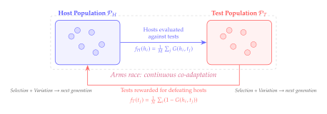
The most dramatic form of coevolution is competitive: two populations are locked in an adversarial struggle, each trying to outperform the other. The canonical biological metaphor is the host–parasite relationship, in which hosts evolve defences against parasites, and parasites evolve countermeasures to circumvent those defences. In computational terms, one population generates solutions and the other generates tests (or adversaries), and each is rewarded for defeating the other.
Historical Note.
Hillis and Co-evolving Sorting Networks (1990). The seminal work on competitive coevolution in computation is due to W. Daniel Hillis [12], who sought to evolve sorting networks – circuits that sort a fixed number of inputs using a sequence of compare-and-swap operations. The key innovation was to co-evolve two populations simultaneously: a population of sorting networks (the “hosts”) and a population of test cases (the “parasites”). The sorting networks were rewarded for correctly sorting as many test cases as possible, while the test cases were rewarded for not being sorted correctly, that is, for exposing failures in the sorting networks.
The results were striking. Sorting networks evolved against a fixed set of random test cases quickly plateaued, learning to sort the specific tests they were given but failing on unseen inputs. In contrast, networks co-evolved with parasitic test cases were driven to ever-greater generality, because any weakness in a network would be exploited by the co-evolving parasites. Hillis reported that the co-evolved networks matched the best known human-designed networks for 16-input sorting, achieving this through an entirely automated process.
Historical Note.
Sims and Virtual Creatures (1994). Karl Sims [13] extended competitive coevolution into the realm of embodied agents. He evolved populations of virtual three-dimensional creatures, represented as graphs of rigid body segments connected by joints with neural network controllers, that competed for possession of a resource (a cube placed between them in a simulated physical environment). The creatures co-evolved both their morphologies and their control strategies, producing an extraordinary menagerie of locomotion strategies, grappling behaviours, and evasive manoeuvres. Some creatures evolved legs to walk toward the cube; others evolved arms to push competitors away; still others evolved entirely novel body plans with no biological analogue. The work demonstrated that competitive coevolution can drive the emergence of complex, adaptive behaviour without explicit design.
Definition 15 (Competitive Coevolutionary System).
A competitive coevolutionary system consists of:
Two populations (hosts) and (tests/parasites), drawn from respective search spaces and .
An interaction function (or more generally ) that evaluates the outcome of a contest between a host and a test .
Fitness functions defined relative to the opposing population: (HOST Fitness) The host fitness rewards hosts that defeat many tests; the test fitness rewards tests that defeat many hosts.
The critical property is that the fitness of every individual depends on the current composition of the opposing population: fitness is context-dependent rather than absolute.
Key Idea.
Fitness is Relative, Not Absolute. In competitive coevolution, no individual has an intrinsic fitness score. A sorting network that perfectly sorts 99% of all possible inputs has zero fitness if the parasitic test population consists entirely of the 1% of inputs it fails on. Conversely, a mediocre network can have perfect fitness if the test population happens to contain only easy cases. This relativity of fitness is both the greatest strength and the greatest danger of coevolutionary systems: it drives continuous improvement through arms races, but it also opens the door to the pathologies we shall study in Pathologies of Coevolution.
Algorithm 5: Competitive Coevolution.
[t]
- Input: Host space , test space , interaction function , population sizes , generations
- Output: Evolved host population
- Initialise host population randomly from
- Initialise test population randomly from
- for
- // Evaluate hosts against current tests
- for each
- // Evaluate tests against current hosts
- for each
- Selection + variation on hosts
- Selection + variation on tests
- return
The computational cost of alg:evo:competitive-coevolution is dominated by the evaluation step, which requires interaction evaluations per generation. When interactions are expensive (e.g., simulating physical contests between virtual creatures), various sampling strategies can be employed: evaluating each individual against a random subset of the opposing population, or using competitive fitness sharing to select representative opponents [39].
Remark 7 (The Minimax Connection).
The astute reader will recognise that competitive coevolution implements a form of minimax optimisation: (Minimax) The hosts seek to maximise performance across the hardest tests, while the tests seek to minimise host performance. This is precisely the structure underlying Generative Adversarial Networks (GANs), where the generator (host) tries to produce samples that fool the discriminator (test), and the discriminator tries to distinguish real from generated samples. Competitive coevolution can thus be viewed as the population-based, gradient-free ancestor of the GAN framework. The pathologies of coevolution – mode cycling, disengagement, failure to converge – find their echoes in the training instabilities of GANs.
Cooperative Coevolution
Not all coevolution is adversarial. In cooperative coevolution, multiple populations evolve complementary components of a solution, and they are rewarded for working together rather than against each other. The biological inspiration is symbiosis: the mitochondrion and the eukaryotic cell, the flower and the pollinator, the mycorrhizal network and the forest.
The computational motivation is equally compelling: many real-world problems have a natural decomposition into subcomponents, and evolving each subcomponent in a separate population can be far more efficient than evolving monolithic solutions. Consider the design of a robot: one population might evolve the morphology (body shape, limb configuration), another the control policy (neural network weights), and a third the sensor layout. Each population explores its own search space, but fitness is determined by how well the components work together as a complete system.
Definition 16 (Cooperative Coevolutionary System).
A cooperative coevolutionary system consists of:
populations , where population consists of individuals drawn from search space .
A collaboration function that assembles one individual from each population into a complete solution in the solution space .
A global fitness function that evaluates complete solutions.
The fitness of individual in population is determined by assembling it with representatives from the other populations: (COOP Fitness) where is the representative individual from population (typically the current best individual or a random collaborator).
The choice of representatives in (COOP Fitness) is critical. Using the current best individual from each population (the greedy strategy) provides a stable evaluation signal but can lead to co-adaptation to a single partner, missing synergies with alternative collaborators. Using random collaborators provides broader coverage but introduces significant noise into the fitness signal. Potter and De Jong [14] proposed a balanced approach: evaluate each individual with both the current best and a random collaborator, and take the maximum fitness across these evaluations.
Algorithm 6: Cooperative Coevolutionary Genetic Algorithm (CCGA).
[t]
- Input: Subspaces , collaboration function , global fitness , population sizes , generations
- Output: Best complete solution found
- for
- Initialise randomly from
- Set representative random member of
- ; Best solution so far
- for
- for Evolve each subpopulation in turn
- for each
- Update representative
- if
- ;
- return
Proposition 6 (Convergence under Separability).
Consider a cooperative coevolutionary system with populations and a global fitness function that is separable: (Separable) where each depends only on the -th subcomponent. If each subpopulation uses a selection mechanism that satisfies the monotone selection property (individuals with higher fitness have higher expected representation in the next generation), then the best complete solution found by generation satisfies (COOP Monotone) and if each has a finite global optimum , then as with probability 1, provided the variation operators maintain positive probability of generating any solution in each .
Proof.
Under separability, the fitness of individual in population does not depend on the representatives from other populations (the cross-terms vanish): , where the second term is a constant with respect to the selection within population . Thus selection within each population is equivalent to selection under alone, and the evolutionary processes are effectively independent. The monotone selection property ensures is non-decreasing in expectation. Since is updated only when a strict improvement is found (alg:evo:ccga, line 15), (COOP Monotone) holds deterministically. The ergodicity condition (positive probability of generating any solution) ensures that each population eventually visits its global optimum, completing the convergence argument.
Caution.
The Separability Assumption is Rarely Satisfied. The convergence guarantee of Proposition 6 hinges on the separability assumption, which is rarely satisfied in practice. For non-separable fitness functions, cooperative coevolution can converge to solutions that are not globally optimal, because the sequential optimisation of subcomponents ignores interaction effects. Consider a simple non-separable function : optimising with fixed and vice versa can cycle or converge to a saddle point. The richer the interactions between subcomponents, the more fragile the cooperative coevolutionary approach becomes. Methods such as random grouping of variables, adaptive decomposition, and contribution-based collaborator selection [14] have been developed to mitigate these issues.
Example 5 (Cooperative Coevolution for Neural Network Design).
Consider the design of a neural network with three interacting components: (1) the network architecture (number and type of layers), (2) the optimisation hyperparameters (learning rate schedule, weight decay), and (3) the data augmentation strategy. A cooperative coevolutionary approach evolves three populations:
: architectures encoded as variable-length sequences of layer specifications.
: hyperparameter vectors specifying learning rate, momentum, weight decay, batch size, etc.
: augmentation policies encoded as sequences of image transformations with associated magnitudes.
To evaluate architecture , we assemble it with the current best hyperparameters and augmentation policy , train the resulting network for a fixed number of epochs, and measure validation accuracy. This approach reduces the search space dimension dramatically compared to searching over all three components jointly, at the cost of potentially missing interactions between components.
The Game-Theoretic View
The language of coevolution is, at its core, the language of game theory. When two populations interact through a fitness function that depends on both, we have a two-player game. When populations interact, we have a -player game. This connection is not merely metaphorical; it provides a rigorous mathematical framework for understanding when coevolution converges, what it converges to, and why it sometimes fails catastrophically.
Definition 17 (Coevolutionary Game).
A coevolutionary game is a tuple where:
is the strategy space of player (population) .
is the utility function (fitness function) of player .
For competitive coevolution with two players, (zero-sum game). For cooperative coevolution, (common-payoff game).
Definition 18 (Coevolutionary Nash Equilibrium).
A strategy profile is a coevolutionary Nash equilibrium if no player can improve their fitness by unilateral deviation: (NASH) Equivalently, is a best response to the strategies of all other players.
Theorem 3 (Convergence of Coevolutionary Dynamics under Monotone Games).
Consider a two-player coevolutionary game (zero-sum) where and are compact convex sets, and the game operator defined by (GAME Operator) is monotone: (Monotone) and strictly monotone (with strict inequality when ). Then:
The game has a unique Nash equilibrium .
Coevolutionary dynamics that implement a best-response process, updating each population toward the best response to the current opposing population, converge to .
The convergence rate depends on the modulus of strong monotonicity: if is -strongly monotone with -Lipschitz gradient, then the distance to equilibrium contracts at rate per generation .
Proof sketch.
Under strict monotonicity, the variational inequality for all has a unique solution by the Minty–Browder theorem. This solution is the Nash equilibrium. The best-response dynamics can be viewed as a forward–backward splitting algorithm applied to the monotone operator , which converges under monotonicity. Under -strong monotonicity, the Banach contraction mapping theorem gives the linear convergence rate with ratio , since the best-response map is a contraction with this constant.
Remark 8 (When Monotonicity Fails).
The monotonicity condition in Theorem 3 is sufficient but far from necessary. Many interesting coevolutionary games are non-monotone, and their dynamics can exhibit the rich pathological behaviours we explore in Pathologies of Coevolution: limit cycles, chaotic attractors, and trajectories that wander through strategy space without ever approaching an equilibrium. The connection between the abstract theory of monotone operators and the concrete pathologies of coevolution is one of the most beautiful bridges between classical mathematics and computational intelligence.
Insight.
From Coevolution to GANs and Back. The minimax formulation of (Minimax) is precisely the objective of a Generative Adversarial Network: . The generator and discriminator are the two “populations” (though each is a single network), and training alternates between updating each, a form of best-response dynamics. The convergence theorems for coevolutionary games directly apply to GAN training when the game operator is monotone. The training instabilities of GANs (mode collapse, oscillation, non-convergence) are manifestations of the coevolutionary pathologies that have been studied in the evolutionary computation literature since the 1990s, decades before GANs were invented. The remedies are often analogous: historical averaging (the coevolutionist's “hall of fame”), spectral normalisation (a form of Lipschitz constraint on the game operator), and unrolled optimisation (multi-step best response).
Exercise 14.
Consider the coevolutionary game of rock–paper–scissors, where (the probability simplex in ) and the payoff matrix is (RPS Payoff)
Show that the unique Nash equilibrium is .
Compute the game operator and verify that it is not monotone.
Simulate best-response dynamics starting from , , and show that the dynamics cycle around the Nash equilibrium without converging.
Propose a modification (e.g., averaging over history) that achieves convergence.
Pathologies of Coevolution
Coevolution promises an arms race that drives continuous improvement. But promises, in the world of adaptive systems, are treacherous things. The same feedback loops that enable spectacular emergent complexity can also trap populations in vicious cycles, drive them into mutual irrelevance, or seduce them into mediocre equilibria from which escape is exponentially difficult. Understanding these pathologies is not merely an academic exercise; it is essential for anyone who seeks to build reliable coevolutionary systems, or equivalently, stable adversarial training procedures for modern generative models.
This section catalogues the four great pathologies of coevolution, each a distinct failure mode with its own mathematical signature, and then presents the arsenal of remedies that the field has developed over three decades of struggle.
Cyclic Dynamics: The Red Queen Trap
The Red Queen Trap takes its name from Lewis Carroll's Through the Looking-Glass, in which the Red Queen tells Alice, “It takes all the running you can do, to keep in the same place.” In coevolutionary systems, this manifests as a situation where both populations are evolving furiously but making no objective progress; they are running faster and faster on a treadmill, each adapting to the other's latest strategy without ever reaching a state that is objectively better than where they started.
The mathematical root of cycling is intransitivity: strategy A beats strategy B, B beats C, and C beats A. When the strategy space contains intransitive cycles, the coevolutionary dynamics can chase their own tail indefinitely.
Definition 19 (Intransitive Superiority).
A set of strategies exhibits intransitive superiority under interaction function if there exists a cyclic sequence of dominance relations: (Intransitive) where denotes that defeats . Equivalently, the dominance relation induced by is not a total order on the strategy space; it contains cycles.
Example 6 (Rock–Paper–Scissors in Coevolution).
The simplest intransitive system is rock–paper–scissors: Rock crushes Scissors, Scissors cuts Paper, Paper covers Rock. Now imagine two populations co-evolving strategies in this game. If the host population converges on Rock, the test population evolves toward Paper. But once the test population is dominated by Paper, the host population shifts toward Scissors. This provokes the test population to shift toward Rock, which causes the hosts to shift back toward Paper, and the cycle continues without end. At no point does either population “improve” in any absolute sense; each is simply chasing the other around the intransitive cycle.
Proposition 7 (Persistence of Intransitive Dynamics).
Consider a coevolutionary system with strategy spaces and an interaction matrix with . If is skew-symmetric ( for all , with ) and , then:
The unique Nash equilibrium in mixed strategies is the uniform distribution (provided is non-degenerate).
The replicator dynamics (Replicator) admit the Nash equilibrium as a fixed point, but this fixed point is Lyapunov stable yet not asymptotically stable: orbits near the equilibrium cycle around it on closed curves (level sets of the function ) without converging.
Discrete-time best-response dynamics can produce periodic orbits of any period dividing , and for generic initial conditions, the dynamics visit each pure strategy infinitely often without settling.
Proof sketch.
The skew-symmetry of ensures that for all , so the game is zero-sum. The Nash equilibrium is found by solving the linear complementarity problem, which for skew-symmetric matrices with full support yields the uniform distribution. The function is a constant of motion under the continuous-time replicator dynamics (as can be verified by direct computation of ), implying that orbits are confined to level sets of and hence cannot converge to the equilibrium from any non-equilibrium initial condition. The discrete-time result follows from the periodicity of best-response correspondences on cyclic dominance structures.
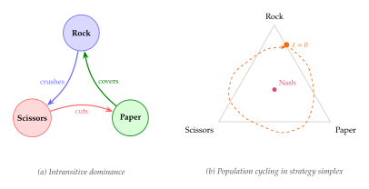
Disengagement
If cycling is the pathology of evenly matched populations chasing each other in circles, disengagement is the pathology of mismatched populations giving up on each other entirely. Disengagement occurs when one population becomes so dominant that the opposing population can no longer provide a useful fitness signal.
Definition 20 (Disengagement).
A coevolutionary system exhibits disengagement at generation if the interaction outcomes become nearly uniform: (Disengagement) for some constant . When , all hosts defeat all tests (host dominance); when , all tests defeat all hosts (test dominance). In either case, the fitness function (eq:evo:host-fitness,eq:evo:test-fitness) assigns nearly identical scores to all individuals in the dominated population, destroying the selection gradient.
Think of it this way: a strong chess player who trains exclusively against weak opponents will gradually lose the tactical sharpness needed to compete at a high level. The training signal – easy victories – provides no pressure to maintain complex strategies, and the cognitive resources devoted to deep tactical calculation are gradually reallocated to simpler pattern matching that suffices against the current opponents. The same dynamic plays out in coevolutionary systems, often with dramatic consequences for the long-term trajectory of the search.
The analogy to mode collapse in GANs is precise. When the generator in a GAN collapses to a single mode that consistently fools the discriminator, the discriminator sees only “fake” samples from that mode and “real” samples from the full data distribution. The discriminator easily learns to reject everything from the collapsed mode, which provides no useful gradient to the generator about how to diversify. Conversely, if the discriminator becomes trivially good (perfectly classifying all samples), the generator receives a saturated gradient signal that provides no directional information. Both scenarios are forms of disengagement.
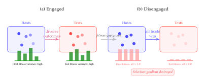
Proposition 8 (Disengagement under Fitness Gap).
Consider a competitive coevolutionary system where the interaction function is continuous, and let denote the mean interaction outcome at generation : (MEAN Interaction) If selection pressure in each population is proportional to fitness (proportionate selection) and the populations use mutation with bounded step size , then disengagement occurs when the fitness gap exceeds the variation radius: there exists a threshold depending on and the population sizes such that (Disengage Threshold) where is arbitrarily small. Informally: when one population dominates by a margin exceeding , the dominated population loses its selection gradient and cannot recover through small mutations alone.
Proof sketch.
Under proportionate selection with bounded mutation, the maximum fitness difference achievable in one generation within the dominated population is . When is near 0 or 1, the variance of the fitness distribution within the dominated population is by the properties of Bernoulli random variables. Setting for an appropriate constant ensures that the fitness variance falls below the selection noise floor, making all individuals in the dominated population effectively equivalent under selection.
Exercise 15.
Implement a competitive coevolutionary system where hosts are neural networks and tests are input vectors , with interaction . Experiment with different population sizes and mutation rates, and measure the frequency and duration of disengagement episodes. Can you identify the critical fitness gap threshold empirically?
Forgetting: The Loss of Hard-Won Knowledge
Perhaps the most insidious pathology of coevolution is forgetting: a population that has learned to defeat a particular class of opponents gradually loses that capability as the opposing population evolves away from those strategies. The hosts learn to beat parasites of type A, so the parasites evolve into type B. The hosts adapt to beat type B, but in doing so, they unlearn their defences against type A. If the parasites ever cycle back to type A, the hosts are as vulnerable as they were at the beginning.
This is the coevolutionary analogue of catastrophic forgetting in neural network training, where learning new tasks overwrites the representations learned for previous tasks. The parallel is not merely metaphorical: in both cases, a system with finite capacity optimises for the current distribution of challenges, sacrificing performance on previously mastered challenges that are no longer present in the training signal. The remedies, too, are analogous: experience replay in continual learning corresponds to the Hall of Fame in coevolution; elastic weight consolidation corresponds to fitness regularisation against archived opponents; progressive network expansion corresponds to growing the solution representation to accommodate new strategies without overwriting old ones.
Definition 21 (Coevolutionary Forgetting).
Let denote the test population at generation , and let denote the best host at generation . The system exhibits coevolutionary forgetting if there exist generations such that:
performs well against : for some threshold .
performs well against but poorly against : for some .
The test population returns to a distribution similar to at generation , and the current best host again performs poorly: .
Forgetting is catastrophic when and the host has lost essentially all capability against the earlier test strategies.
Remark 9 (Forgetting and Finite Capacity).
Forgetting is fundamentally a consequence of finite representational capacity. If the host solution space is rich enough to simultaneously encode strategies for defeating all possible test types, forgetting need not occur. In practice, however, solutions have bounded complexity (limited network size, finite program length, fixed number of parameters), and the capacity allocated to countering one type of opponent must be repurposed to counter another. This is identical to the capacity argument in continual learning: a neural network with parameters can represent at most independent task solutions before interference becomes inevitable.
Example 7 (Forgetting in Coevolved Game Strategies).
Consider co-evolving strategies for the iterated Prisoner's Dilemma with memory-1 (strategies that condition on the previous round's outcome). The strategy space consists of four probabilities: , specifying the probability of cooperating after (CC), (CD), (DC), and (DD) respectively, where the first letter is the player's own previous action.
In a typical coevolutionary run, the following forgetting cycle emerges:
Generations 1–50: Hosts evolve toward Tit-for-Tat (), which defeats the initially random test strategies.
Generations 50–150: Tests evolve toward Always-Cooperate (), exploiting Tit-for-Tat's willingness to cooperate. Hosts drift toward Always-Defect (), which maximises payoff against cooperators.
Generations 150–250: Tests evolve retaliatory strategies (similar to Tit-for-Tat). Hosts have forgotten how to cooperate and are trapped in mutual defection.
Generations 250+: The cycle repeats, with hosts rediscovering cooperation, then forgetting it, in a pattern that shows no long-term progress.
The performance of the generation-250 hosts against the generation-50 tests is worse than the performance of the generation-50 hosts against those same tests, despite 200 additional generations of evolution. This is forgetting in action.
Exercise 16.
Design an experiment to measure coevolutionary forgetting. Maintain an archive of test populations from every -th generation. After the evolution finishes, evaluate the final best host against each archived test population. Plot the host's performance as a function of the age of the test population. A monotonically decreasing curve indicates progressive forgetting; a U-shaped curve suggests selective forgetting of intermediate strategies.
Mediocre Stable States
The most frustrating pathology of all is the mediocre stable state: a configuration in which both populations have settled into a lukewarm equilibrium, each performing adequately but not brilliantly against the other, and neither having any incentive to change. Unlike a Nash equilibrium, which represents a genuinely optimal configuration (no player can improve by unilateral deviation), a mediocre stable state is a trap, a configuration that appears stable but is far from optimal, and from which escape requires coordinated changes in both populations that are exponentially unlikely under independent variation.
Definition 22 (Mediocre Stable State).
A coevolutionary state is a mediocre stable state if:
It is locally stable: small perturbations to either population (adding or removing a few individuals, applying small mutations) do not change the fitness ranking within either population, so the selection dynamics return to .
It is globally suboptimal: there exist strategies and such that and , but performs worse than against (and similarly for against ).
It is not a Nash equilibrium: there exist strategies that would be better responses if the opposing population also changed, but that appear inferior under the current opposing population.
Proposition 9 (Exponential Escape Time from Mediocre Stable States).
Consider a coevolutionary system with binary strategy spaces and an interaction function such that the optimal strategy pair differs from the mediocre stable state in at least bit positions in each component. Under mutation rate per bit and population size , the expected number of generations to escape the mediocre stable state is (Mediocre Escape) When , that is, when the optimal solution differs from the mediocre state in a constant fraction of positions, the escape time is exponential in the problem dimension: for some constant .
Proof sketch.
For the host population to escape the basin of attraction of the mediocre state, at least one individual must simultaneously differ from in specific positions (those that correspond to the path toward the optimal strategy). Under independent bit-flip mutation with rate , the probability of flipping exactly the right bits while leaving the other bits unchanged is . With population size , the expected waiting time for any individual to achieve this is . Crucially, this mutation must survive selection, but by the definition of a mediocre stable state, such a mutant appears inferior under the current test population, so it is likely to be selected against. Escape thus requires not only the right mutation in the host population but also a compatible mutation in the test population, compounding the exponential difficulty.
Caution.
Mediocre Stable States Are Invisible. The most dangerous property of mediocre stable states is that they are undetectable from within the coevolutionary system. Both populations appear to have converged; fitness values are stable; there is no selection pressure for change. An observer monitoring only the internal fitness dynamics would conclude that the system has found a satisfactory solution. Only by evaluating the evolved solutions against an external benchmark, a fixed, absolute fitness function, can the mediocrity be revealed. This is why maintaining external evaluation alongside coevolutionary fitness is essential in practice.
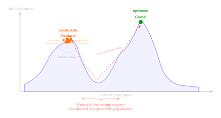
Solutions to Pathologies
Three decades of wrestling with coevolutionary pathologies have produced a rich toolkit of remedies. No single technique solves all problems, but the combination of several can produce coevolutionary systems that are remarkably robust.
Definition 23 (Hall of Fame).
A Hall of Fame (HoF) is an archive that stores the best individuals from previous generations. The fitness of a current individual is evaluated not only against the current opposing population but also against the archived opponents: (HOF Fitness) where is the archive of past test individuals and controls the balance between adapting to current opponents and maintaining competence against historical ones.
The Hall of Fame directly addresses forgetting: by requiring hosts to perform well against archived tests from earlier generations, it prevents them from unlearning previously acquired capabilities. It also mitigates cycling: if the test population cycles back to a previously seen strategy, the archive already contains that strategy, and hosts that have forgotten how to beat it are penalised.
Algorithm 7: Hall of Fame Coevolution.
[t]
- Input: Host space , test space , interaction , archive sizes , balance , generations
- Output: Evolved host population
- Initialise , randomly
- ; Archives
- for
- // Evaluate with Hall of Fame
- for each
- (skip if )
- (Analogous evaluation for tests against host archive )
- ; trim to size
- ; trim to size
- return
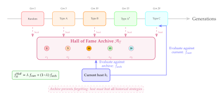
Shared Fitness and Competitive Fitness Sharing.
Fitness sharing [39] modifies the fitness of a test individual to reward uniqueness: a test that defeats few hosts (but defeats them uniquely, since no other test can defeat them) receives higher fitness than a test that defeats many hosts but is redundant with other tests. Formally, the shared fitness of test is (Competitive Fitness Sharing) where the denominator counts how many other tests also defeat host . This encourages the test population to maintain diversity, covering different weaknesses of the host population rather than converging on a single exploit. The effect is analogous to diverse ensemble training in machine learning: each test specialises in exposing a different vulnerability.
Pareto Coevolution.
Ficici and Pollack [40] proposed treating coevolution as a multi-objective optimisation problem: instead of aggregating performance across all opponents into a single scalar, treat performance against each opponent (or class of opponents) as a separate objective, and apply Pareto-based selection. A host dominates another host if performs at least as well as against every test, and strictly better against at least one. The Pareto front of non-dominated hosts is preserved, maintaining a diverse set of strategies that collectively cover the space of possible opponent types.
This approach is particularly effective against mediocre stable states, because Pareto selection preserves “specialist” strategies that excel against particular opponents even if they perform poorly on average. These specialists serve as stepping stones that can eventually be combined (through crossover or other variation) into generalist strategies that escape the mediocre equilibrium.
| Pathology | Signature | Root Cause | Remedies |
| Cyclic dynamics (Cyclic Dynamics: The Red Queen Trap) | Periodic oscillations in population strategy composition; no improvement on external benchmark | Intransitive dominance structure in strategy space | Hall of Fame; fitness sharing; Pareto coevolution; increased population diversity |
| [6pt] Disengagement (Disengagement) | Near-uniform fitness within one population; interaction outcomes nearly constant | Fitness gap exceeds variation radius; one population dominates completely | Asymmetric mutation rates; competitive fitness sharing; resource sharing; diversity injection |
| [6pt] Forgetting (Forgetting: The Loss of Hard-Won Knowledge) | Performance against archived opponents degrades over time; periodic regression | Finite representational capacity; no memory of past opponents | Hall of Fame; experience replay; growing solution capacity; multi-objective evaluation |
| [6pt] Mediocre stable states (Mediocre Stable States) | Stable fitness with no improvement; poor absolute performance; appears converged | Local stability without global optimality; escape requires coordinated multi-population change | Pareto coevolution; novelty-based diversity; random restarts; external fitness evaluation |
Exercise 17.
Implement a competitive coevolutionary system for a simple game (e.g., iterated Prisoner's Dilemma with memory-1 strategies). Run the system for 1000 generations and instrument it with the following diagnostics:
Cycling detector: Track the centroid of each population's strategy distribution and compute its autocorrelation. High autocorrelation at lag indicates cycling with period .
Disengagement detector: Monitor the variance of fitness within each population. A drop below a threshold signals disengagement.
Forgetting detector: Maintain an archive of past opponents and periodically evaluate the current best against the archive. Declining performance indicates forgetting.
External fitness: Evaluate the current best against a fixed, comprehensive test suite not used in coevolution. Stagnation on this metric despite active coevolution suggests a mediocre stable state.
Report which pathologies you observe and at what generations they occur. Then apply the Hall of Fame remedy and repeat.
Quality-Diversity and MAP-Elites
We arrive now at what may be the most philosophically provocative idea in all of evolutionary computation: the suggestion that the goal of evolution is not to find the best solution, but to find all the interesting ways to solve a problem.
For four decades, evolutionary algorithms have been framed as optimisation procedures. The objective is always the same: maximise (or minimise) a fitness function. Find the tallest peak in the landscape. Get to the top. Plant a flag. Declare victory. This framing is so deeply embedded in the culture of evolutionary computation, and indeed in the broader culture of computer science, that it is difficult to imagine an alternative. But nature, as always, provides one.
Consider the biosphere. Evolution has not produced a single “optimal” organism. It has produced an astonishing diversity of organisms, each adapted to a different ecological niche: bacteria that thrive in boiling acid, fungi that digest rock, whales that navigate by song, birds that fly backwards. This diversity is not a failure of optimisation. It is the product of a process that rewards novelty and exploration as much as performance, and the diversity itself is the source of the biosphere's resilience, adaptability, and creative potential.
The quality–diversity (QD) paradigm [16] translates this insight into a computational framework. Instead of seeking a single best solution, QD algorithms seek a diverse collection of high-performing solutions, each occupying a distinct region of a user-defined “behaviour space.” The result is not a single answer but a repertoire, a library of solutions that collectively illuminate the space of possibilities.
Key Idea.
Quality-Diversity: A Library, Not a Book. Traditional optimisation is like searching for the best book in a library: you want the single volume that most perfectly addresses your question. Quality–diversity is like building the library: you want a rich collection of books spanning every subject, genre, and perspective, with each shelf holding the best book on its particular topic. The library is more valuable than any individual book, because it provides answers to questions you have not yet thought to ask.
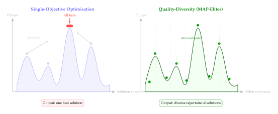
Beyond Optimisation: The Quality-Diversity Paradigm
Why would we want diversity rather than (or in addition to) optimality? Three compelling reasons:
Robustness.
A single optimal solution is brittle: if the problem changes slightly (a new constraint, a shifted objective, a perturbation in the environment), the solution may become useless. A diverse repertoire is robust: among the hundreds of solutions it contains, there is likely one that remains effective under the new conditions. This is the evolutionary analogue of the maxim “don't put all your eggs in one basket.”
Stepping Stones.
Solutions that are suboptimal for the current problem may be essential stepping stones toward solutions that are optimal for a harder variant. Fitness landscapes are often deceptive: the path to the global optimum leads through regions of low fitness. By maintaining a diverse repertoire, QD algorithms preserve these stepping-stone solutions, enabling future discovery that a greedy optimiser would foreclose. This is the deep insight of Lehman and Stanley's work on novelty search [8], which we explore in Novelty Search.
Insurance Against Uncertainty.
When we do not know exactly what problem we will face in the future, having a repertoire of qualitatively different solutions is a form of insurance. In robotics, for example, a repertoire of diverse locomotion behaviours allows a damaged robot to quickly adapt by selecting a pre-computed behaviour that does not rely on the damaged component [15].
Definition 24 (Quality-Diversity Problem).
A quality–diversity problem is defined by:
A solution space .
A fitness function (quality) that measures the performance of each solution.
A behaviour descriptor function that maps each solution to a point in a -dimensional behaviour space.
The goal is to find a repertoire such that: itemize
The repertoire covers the behaviour space: the descriptors span as uniformly as possible.
Each solution in the repertoire is high-quality: is as large as possible for its behaviour region. itemize
The objective is simultaneously to illuminate the behaviour space (discover all achievable behaviours) and to optimise within each behavioural niche (find the best solution for each behaviour).
Novelty Search
Before MAP-Elites, there was an even more radical idea: what if we abandoned the fitness function entirely?
In 2011, Joel Lehman and Kenneth Stanley [8] proposed novelty search, a paradigm that replaces fitness-based selection with selection for behavioural novelty. Instead of rewarding solutions that perform well, novelty search rewards solutions that behave differently from anything seen before. The fitness function is not merely modified or supplemented; it is discarded. The only selection pressure is toward the new, the unexplored, the different.
The philosophical audacity of this proposal cannot be overstated. It flies in the face of four decades of optimisation-centric thinking. And yet, on certain classes of problems, specifically problems with deceptive fitness landscapes, novelty search dramatically outperforms fitness-based search.
Definition 25 (Novelty Search).
Novelty search replaces the fitness function with a novelty score computed as follows:
Each solution is characterised by its behaviour descriptor .
An archive of previously encountered behaviours is maintained.
The novelty of is the average distance from to its -nearest neighbours in the archive (combined with the current population): (Novelty) where are the nearest neighbours of in under the behaviour-space distance.
Solutions with (a threshold) are added to the archive.
Selection is based on rather than any task-specific fitness function .
Proposition 10 (Novelty Search and Deceptive Problems).
Consider a search space with a fitness function that is deceptive: the gradient of (in the neighbourhood structure of ) points away from the global optimum in a region containing all local optima. Formally, let be the global optimum, and suppose there exists a basin such that for all , all neighbours of with satisfy . Then:
Any fitness-based search that follows the fitness gradient will be repelled from and trapped in a local optimum outside it.
Novelty search, which ignores entirely, explores the behaviour space uniformly and will eventually place solutions inside , discovering or a high-quality solution near it.
The expected number of evaluations for novelty search to reach is , where is the number of distinct behavioural niches needed to cover the space, independent of the deceptiveness of .
Proof sketch.
Part (1) follows directly from the definition of deceptiveness: any greedy ascent on moves away from once the trajectory reaches . For part (2), novelty search uniformly covers the behaviour space because each new solution added to the archive pushes subsequent solutions toward unexplored regions. By a coupon-collector argument over behavioural niches, the expected time to cover all niches (including those inside ) is . Part (3) refines this to by noting that novelty search adds solutions to underrepresented regions with probability proportional to their deficit, giving linear rather than coupon-collector scaling in the number of niches.
Insight.
The Path to Your Goal May Lead Away From It. Novelty search embodies a profound and counterintuitive insight: sometimes the best way to reach your goal is to stop trying to reach it. When the fitness landscape is deceptive, every step toward “better” takes you farther from “best.” By abandoning the fitness function and instead seeking only novelty, exploring for its own sake without any notion of progress toward a goal, you cover the space of possibilities uniformly, and in doing so, you stumble upon solutions that goal-directed search could never reach.
This is not merely a computational trick. It is a deep statement about the nature of creative discovery. The most important scientific breakthroughs, artistic innovations, and engineering achievements often came not from the relentless pursuit of a defined objective, but from curiosity-driven exploration that led to unexpected places. Penicillin was discovered by accident. The microwave oven was invented by a radar engineer who noticed his chocolate bar melting. The theory of general relativity emerged from Einstein's thought experiments about riding on a beam of light, not from any systematic attempt to improve Newtonian mechanics. Novelty search is the algorithmic formalisation of this insight.
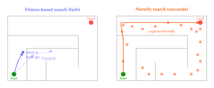
MAP-Elites
Novelty search demonstrated that abandoning fitness in favour of behavioural diversity can be powerful. But it goes too far: by ignoring fitness entirely, novelty search discovers many diverse solutions but makes no guarantee about their quality. What we really want is both: diversity and quality. Enter MAP-Elites.
The Multi-dimensional Archive of Phenotypic Elites (MAP-Elites) [15] is an elegantly simple algorithm that maintains a map (grid) of the highest-performing solution discovered for each cell in a discretised behaviour space. It simultaneously optimises quality within each behavioural niche and maintains diversity across niches, producing a structured repertoire that “illuminates” the relationship between behaviour and performance.
Definition 26 (MAP-Elites Archive).
The MAP-Elites archive is a data structure defined on a grid that discretises the -dimensional behaviour space into cells: (GRID) where is the number of bins along behaviour dimension . Each cell either is empty () or contains the elite, the highest-fitness solution whose behaviour descriptor falls within that cell: (Elite) where maps continuous behaviour descriptors to grid cells.
Algorithm 8: MAP-Elites.
[t]
- Input: Solution space , fitness , behaviour descriptor , grid , initial batch size , total evaluations
- Output: MAP-Elites archive
- for all Initialise empty archive
- // Initialisation: random solutions
- for
- Determine behaviour cell
- if
- Place or replace elite
- // Main loop: variation and illumination
- for
- random occupied cell's elite from Select parent
- Generate offspring via variation
- Evaluate and
- if
- return
The beauty of MAP-Elites lies in its simplicity. The algorithm (alg:evo:map-elites) has only two operations: generate a random variation of an existing elite, and place it in the archive if it is either the first solution in its cell or better than the current occupant. There is no explicit population, no selection tournament, no crossover pool. The archive is the population, and the grid structure provides both diversity maintenance (solutions in different cells are preserved regardless of relative fitness) and quality pressure (within each cell, only the best solution survives).
Remark 10 (Properties of MAP-Elites).
MAP-Elites exhibits several remarkable properties:
Illumination: Over time, the archive fills with solutions, “lighting up” the behaviour space and revealing which behaviours are achievable and how well they can be performed. The filled archive is itself a scientific instrument for understanding the problem.
Stepping stones: A solution placed in one cell can serve as a parent for offspring that land in distant cells, providing stepping-stone paths through behaviour space that would be inaccessible to a fitness-only search.
Monotone improvement: The fitness of the elite in each cell is non-decreasing over time, since updates only occur when a strictly better solution is found.
Anytime algorithm: MAP-Elites can be stopped at any time and returns a useful (if incomplete) repertoire. More computation always improves the result.
Embarrassingly parallel: Multiple workers can independently generate and evaluate offspring, submitting updates to a shared archive with a simple compare-and-swap operation.
Example 8 (MAP-Elites for Robot Locomotion).
Consider a hexapod robot with 18 joints (3 per leg), and suppose we want a repertoire of walking gaits. The solution space is the space of open-loop gait controllers (e.g., parameters of a central pattern generator). The fitness function is the walking speed. The behaviour descriptor is a 6-dimensional binary vector indicating which legs are in contact with the ground during the gait cycle (yielding possible “gait types,” from one-legged hopping to six-legged crawling).
MAP-Elites produces a repertoire of 64 gaits, each the fastest discovered gait of its type. This repertoire is invaluable for damage recovery: if the robot loses a leg, it can instantly switch to the best gait that does not use that leg, achieving graceful degradation without any re-learning. Mouret and Clune [15] demonstrated that a damaged hexapod using MAP-Elites could recover effective locomotion in under two minutes of real-time adaptation.
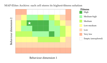
Proposition 11 (Monotone Archive Quality).
Let denote the MAP-Elites archive after evaluations, and define the archive quality as (Archive Quality) Then is non-decreasing in : (Quality Monotone) Similarly, the coverage is non-decreasing.
Proof.
By the update rule in alg:evo:map-elites (lines 6–7 and 14–15), a cell's occupant is only replaced by a solution with strictly higher fitness. Therefore, the fitness of every occupied cell is non-decreasing, and cells never become empty once occupied. The sum inherits these monotonicity properties.
Exercise 18.
Implement MAP-Elites for a continuous optimisation problem of your choice (e.g., the Rastrigin function in ). Define the behaviour descriptor as the solution coordinates themselves (a trivial choice that makes the MAP-Elites grid a discretisation of the search space). Visualise the archive at different stages of the search (after 100, 1000, and 10000 evaluations) as a heatmap. Compare the best solution found by MAP-Elites with the best found by a standard evolutionary algorithm with the same evaluation budget. Is the MAP-Elites solution competitive? When is it better?
Exercise 19.
The choice of behaviour descriptor is critical to the success of MAP-Elites. For the problem of evolving neural network architectures:
Propose three different behaviour descriptors that capture qualitatively different aspects of architecture behaviour (e.g., computational cost, representation geometry, gradient flow statistics).
Argue which descriptor would produce the most useful repertoire for a practitioner.
Discuss the trade-off between behaviour space dimensionality and archive coverage: what happens when is too large?
Connections to Generative Models
The quality–diversity framework has a deep and illuminating connection to generative modelling that goes beyond mere analogy. A MAP-Elites archive can be viewed as an implicit generative model over the solution space: by sampling uniformly from the occupied cells of the archive, we obtain a distribution over solutions that is both diverse (covering the behaviour space) and high-quality (each sample is the best known solution for its behavioural niche). This perspective opens the door to a powerful fusion of QD algorithms and deep generative models.
Quality-Diversity as Implicit Generative Model.
Consider a MAP-Elites archive with occupied cells. Sampling a solution from this archive produces a random variable , where (Archive Distribution) This is a uniform mixture of point masses, one at each elite. As the archive grows (more cells become occupied and elites improve), this implicit distribution becomes a richer and more accurate model of the space of high-performing, diverse solutions. In the limit where the grid resolution approaches the intrinsic dimensionality of the behaviour space, the archive distribution converges to a continuous distribution supported on the Pareto front of quality vs. diversity.
Differentiable Quality-Diversity (DQD).
The limitation of standard MAP-Elites is that it uses random, undirected variation: mutations are sampled without knowledge of the fitness landscape or the behaviour descriptor function. When the solution space is parameterised by a differentiable model (e.g., a neural network), we can compute gradients of both the fitness and the behaviour descriptor with respect to the parameters, enabling directed variation that moves solutions toward better quality and toward under-explored regions of behaviour space.
Definition 27 (Differentiable Quality-Diversity).
A Differentiable Quality-Diversity (DQD) algorithm augments MAP-Elites with gradient information. For a solution parameterised by with differentiable fitness and behaviour descriptor , the DQD update generates offspring by: (DQD Update) where is the quality step size, is the Jacobian of the behaviour descriptor, is a desired behaviour displacement (pointing toward empty or underrepresented cells), and controls the exploration intensity. The first term improves quality; the second term drives exploration of under-populated behaviour regions.
The DQD framework provides a principled way to combine the strengths of gradient-based optimisation (fast convergence to local optima) with the strengths of QD algorithms (diversity maintenance and global exploration). It is particularly powerful when the solution space is high-dimensional and random mutations are inefficient, precisely the regime where deep generative models operate.
Latent Space Illumination.
An even more powerful approach uses a deep generative model, typically a variational autoencoder (VAE), to learn a low-dimensional latent space that parameterises the solution space, and then performs MAP-Elites in this latent space rather than in the original parameter space. The VAE is trained on solutions discovered during the QD search, creating a learned mapping from a compact latent code (with ) to solutions , where is the decoder.
The advantages are twofold:
Efficient variation: Mutations in the low-dimensional latent space produce semantically meaningful variations in solution space, because the VAE has learned the manifold of valid solutions. This is the QD analogue of the LLM-guided mutation we studied in LLMs as Semantic Variation Operators.
Interpolation: The latent space supports smooth interpolation between solutions, enabling the generation of novel solutions that “blend” the characteristics of existing elites.
Conjecture 2 (QD-VAE Convergence).
Let be a VAE decoder trained on the current MAP-Elites archive, and let MAP-Elites be run in the latent space using Gaussian mutations , . If the VAE is retrained periodically as the archive grows, and the latent dimension is sufficient to capture the intrinsic dimensionality of the solution manifold, then the archive coverage rate (cells filled per evaluation) of latent-space MAP-Elites exceeds that of direct-space MAP-Elites by a factor of asymptotically.
Remark 11 (QD LLMs: The Foundation for AlphaEvolve).
The synthesis of quality–diversity algorithms with large language models creates a framework of extraordinary power. Consider a MAP-Elites archive where each cell contains a program (algorithm, proof, design), the fitness function measures performance on a benchmark, and the behaviour descriptor captures structural or functional properties of the program (runtime complexity class, memory usage pattern, algorithmic paradigm). Now replace the random mutation operator with an LLM-guided variation operator that understands the program's structure and can make semantically meaningful modifications.
This is precisely the architecture underlying systems like AlphaEvolve (which we study in detail in later sections): a population of programs is maintained in a diversity-aware archive, and an LLM generates intelligent variations that both improve quality and explore new behavioural niches. The QD framework provides the scaffolding for diversity; the LLM provides the variation quality. The combination produces a system that is simultaneously creative (discovering qualitatively new approaches) and effective (optimising within each approach). This marriage of evolutionary diversity and neural intelligence is, we believe, one of the most promising directions in all of AI.
Exercise 20.
Design a quality–diversity system for generating diverse, high-quality images of a given class (e.g., “chairs”). Specify:
The solution space (e.g., latent codes of a pre-trained generative model).
The fitness function (e.g., classifier confidence, aesthetic score, or FID against a reference set).
The behaviour descriptor (e.g., colour histogram, aspect ratio, number of legs, material texture).
The variation operator (e.g., interpolation in latent space, LLM-guided text prompt modification).
Argue why a QD approach to image generation might produce more useful results than a standard generative model that optimises a single quality metric.
Exercise 21.
Analyse the scaling properties of MAP-Elites as the behaviour space dimensionality increases. If the grid has bins per dimension, the total number of cells is . For and , this gives cells.
What fraction of cells can realistically be filled with evaluations?
Propose modifications to MAP-Elites that handle high-dimensional behaviour spaces (e.g., CVT-MAP-Elites using Centroidal Voronoi Tessellations instead of regular grids).
Prove or disprove: the coverage rate of MAP-Elites (fraction of cells filled per evaluation) decreases exponentially with under uniform random variation.
Open Problem 2.
Open Problems in Quality-Diversity. Several fundamental questions in quality–diversity remain open:
Automatic behaviour descriptor discovery: Current QD methods require the user to specify the behaviour descriptor. Can we learn the descriptor from data, discovering the most “interesting” axes of variation automatically?
Theoretical coverage guarantees: Under what conditions on the fitness landscape and variation operator can we prove that MAP-Elites achieves full coverage of the reachable behaviour space in polynomial time?
QD in non-stationary environments: How should the archive be managed when the fitness function or the environment changes over time? Should old elites be discarded, re-evaluated, or retained as potential stepping stones?
Multi-objective QD: How to extend QD to settings where fitness itself is multi-dimensional, so each cell should store a Pareto front rather than a single elite?
Theorem 4 (Coverage Rate of MAP-Elites).
Let denote the MAP-Elites archive after evaluations on a grid with cells. Suppose the variation operator satisfies the following reachability condition: for every occupied cell and every cell adjacent to in the behaviour space, the probability that an offspring of the elite in lands in is at least . Let be the number of occupied cells at time . Then the expected time to fill all reachable cells satisfies (Coverage Bound) where is the -th harmonic number.
Proof.
The argument proceeds by analogy with the coupon collector problem. When cells are occupied, the probability that the next offspring lands in an unoccupied cell is at least (since the parent is in an occupied cell and has probability at least of reaching any adjacent cell, and at least of its adjacent cells are unoccupied in expectation under a spreading wavefront). The expected time to transition from to occupied cells is therefore at most . Summing over all transitions from to gives (Coverage Proof) The bound is tight up to constant factors when the reachability condition holds uniformly across the grid.
Corollary 2 (Curse of Dimensionality in MAP-Elites).
For a -dimensional behaviour space with bins per dimension (so ), the expected time to achieve full coverage is (Coverage Curse) which grows exponentially in . This is the curse of dimensionality for MAP-Elites: in behaviour spaces of dimension , the standard grid-based archive becomes impractical and must be replaced by adaptive tessellation schemes such as Centroidal Voronoi Tessellation (CVT-MAP-Elites).
Example 9 (CVT-MAP-Elites).
CVT-MAP-Elites replaces the regular grid with a Centroidal Voronoi Tessellation: a set of centroids that partition the behaviour space into Voronoi cells, where each cell contains all points closer to its centroid than to any other. The centroids are computed to minimise the quantisation error: (CVT) The advantage is that the number of cells is chosen by the user independently of the behaviour space dimension , breaking the exponential dependence. The disadvantage is that the tessellation must be precomputed (typically via Lloyd's algorithm) and does not adapt to the density of discovered solutions. In practice, to CVT cells work well for behaviour spaces of dimension , providing sufficient resolution without the combinatorial explosion of regular grids.
The CVT centroids can be computed efficiently using the -means++ initialisation followed by Lloyd's algorithm:
Sample points uniformly from .
Run -means with clusters for 100 iterations.
Use the resulting cluster centres as the CVT centroids.
Cell assignment during MAP-Elites then reduces to a nearest-neighbour query, which can be accelerated to time using a -d tree.
Lemma 1 (Selection Pressure in MAP-Elites).
In MAP-Elites, the implicit selection pressure on an elite in cell is proportional to the number of offspring it generates that successfully enter the archive. Let denote the probability that an offspring of the elite in either enters an empty cell or displaces an existing elite. Then the effective selection probability of cell being chosen as a parent and producing a surviving offspring is (Effective Selection) where is the current number of occupied cells. Cells whose elites have high fitness (making it hard for offspring to displace neighbours) and cells surrounded by empty cells (providing easy targets) have the highest effective selection probability. This creates a natural bias toward frontier exploration: cells at the boundary of the explored region produce more surviving offspring, so they are effectively selected more often.
Historical Note.
The Intellectual Lineage of Quality-Diversity. The quality–diversity paradigm did not emerge from a vacuum. Its intellectual lineage traces through several independent streams:
Fitness sharing and niching (Goldberg & Richardson, 1987): The earliest attempts to maintain diversity in evolutionary algorithms, using shared fitness to prevent convergence to a single peak.
Behavioural diversity (Mouret & Doncieux, 2012): The insight that diversity should be measured in behaviour space (what solutions do) rather than genotype space (how solutions are encoded).
Novelty search (Lehman & Stanley, 2011): The radical proposal to abandon fitness entirely in favour of behavioural novelty, demonstrating that exploration alone can solve deceptive problems [8].
Multi-objective evolutionary algorithms (Deb et al., 2002): NSGA-II and related algorithms that maintain Pareto fronts, providing the technical machinery for simultaneously optimising multiple objectives.
MAP-Elites (Mouret & Clune, 2015): The synthesis that combined behavioural diversity with quality optimisation into a single, elegant framework [15].
Quality-Diversity (Pugh, Soros & Stanley, 2016): The unifying theoretical framework that encompasses novelty search, MAP-Elites, and related algorithms under a single paradigm [16].
Each contribution built upon the previous ones, gradually shifting the field's perspective from “find the best” to “find all the interesting.” This shift mirrors a broader movement in AI from pure optimisation toward open-ended discovery, a movement that finds its most powerful expression in the LLM-guided evolutionary systems we study later in this chapter.
Exercise 22.
Prove the following claim or provide a counterexample: for any fitness function on a finite search space with , novelty search (with archive) visits the global optimum in expected time , regardless of the structure of . Compare this with the expected time for random search () and fitness-proportionate selection ( under certain assumptions). Under what conditions does novelty search outperform both alternatives?
Exercise 23.
Explain the conceptual relationship between competitive coevolution (Competitive Coevolution) and quality–diversity. Specifically:
Show that a Hall of Fame archive in coevolution is analogous to a MAP-Elites archive in QD, where the “behaviour descriptor” is the identity of the opponent.
Argue that competitive fitness sharing ((Competitive Fitness Sharing)) encourages test-population diversity in the same way that the MAP-Elites grid encourages solution diversity.
Propose a hybrid algorithm that uses MAP-Elites to maintain the test population in a competitive coevolutionary system, with the behaviour descriptor being the set of hosts that each test defeats.
Exercise 24.
Consider the MAP-Elites archive as an information-theoretic object. Define the archive entropy as (Archive Entropy) where the sum is over occupied cells.
Show that is maximised when all elites have equal fitness (maximum diversity of quality).
Show that is minimised when a single elite dominates (one cell has much higher fitness than all others).
Propose an alternative QD objective that maximises for some temperature parameter , and discuss how this relates to maximum-entropy reinforcement learning.
LLMs as Semantic Variation Operators
In the preceding sections we developed the classical machinery of evolutionary computation: populations, fitness landscapes, crossover, mutation, and selection. Every one of these ideas traces back to the biological metaphor of blind variation and selective retention, a framework that has powered four decades of remarkably successful optimisation. Yet if we step back and examine the variation operators that drive classical evolutionary algorithms, we discover a fundamental limitation that becomes increasingly severe as we move from continuous numerical optimisation to the structured, discrete, semantically rich domains that matter most in modern AI: code synthesis, mathematical proof discovery, algorithm design, and hardware optimisation.
The limitation is simple to state but profound in its consequences: classical variation operators are structurally blind. They perturb solutions without understanding what those solutions mean.
This section charts the paradigm shift that occurs when we replace blind random mutation with the semantic understanding of large language models. The result is a new class of variation operators that understand syntax, respect semantics, diagnose failure modes, and generate targeted repairs. This fusion of evolutionary search with generative language models is, we shall argue, one of the most consequential developments in AI since the transformer architecture itself.
The Fundamental Limitation of Classical Variation
Consider the task of evolving a sorting algorithm. A candidate solution is a program, represented as a string of characters or an abstract syntax tree. Classical genetic programming applies variation operators drawn from the same conceptual family as the bit-flip mutations and single-point crossovers we studied in LLMs as Semantic Variation Operators: random subtree replacement, point mutations that swap one function symbol for another, and crossover that grafts a subtree from one parent into a random position in another.
The difficulty is immediate. A random subtree replacement in a program is overwhelmingly likely to produce a syntactically invalid result. Even when the result is syntactically valid, it is almost certainly semantically meaningless: the program crashes, enters an infinite loop, or produces output that bears no relation to sorting. Empirical studies of classical genetic programming report that between 70% and 95% of offspring produced by random variation are non-functional [11], a staggering waste of computational effort.
Definition 28 (Classical Variation Operator).
A classical variation operator is a stochastic map that, given a candidate solution in some representation space, produces a modified solution where is a random perturbation drawn from a fixed distribution that is independent of the structure or semantics of . Formally: (Classical Variation) The critical property is the independence : the perturbation distribution does not adapt to the content or structure of the parent solution.
The consequences of structural blindness are most devastating in highly constrained search spaces. Consider the following hierarchy of increasing structural complexity:
Continuous vectors : Gaussian perturbations , , produce valid solutions with probability 1. Classical ES and CMA-ES exploit this property brilliantly.
Combinatorial structures (permutations, graphs): Validity constraints reduce the fraction of useful mutations, but domain-specific operators (swap mutations for permutations, edge insertions for graphs) maintain reasonable survival rates of 30–60%.
Programs and algorithms: The space of syntactically valid, semantically meaningful programs is a vanishingly small subset of the space of all character strings. Random perturbations almost never land in this subset.
Mathematical proofs: Every step must follow logically from previous steps. A random perturbation to a proof step almost certainly breaks the logical chain.
Proposition 12 (Survival Rate Decay in Structured Spaces).
Let be a search space with validity constraint , and let the survival rate of a variation operator be defined as (Survival RATE) where is the current population distribution. For a classical variation operator with uniform random perturbation over a space of syntactic objects of length with alphabet size , the survival rate satisfies (Survival Bound) which decays exponentially in the solution length .
Proof.
Under uniform random perturbation, the output is effectively a random element of the space of all strings of length over alphabet . The probability that a uniformly random string is valid is exactly the ratio . For programming languages with context-free or context-sensitive grammars, the number of valid programs of length grows at most polynomially in for some , yielding the exponential decay bound.
The needle-in-a-haystack problem.
For a concrete illustration, consider Python programs of length characters. The ASCII alphabet has printable characters, giving possible strings. The number of syntactically valid Python programs of this length is astronomically smaller, and the number that are syntactically valid, terminate, and compute something useful for a given task is smaller still. A random mutation that changes even a single character has a high probability of producing a syntax error, a runtime exception, or a program that computes an entirely different function. Classical genetic programming copes with this by using tree-based representations and type-constrained operators, but these are band-aids on a fundamental wound: the variation operator does not understand what the program does.
The Paradigm Shift: LLMs as Intelligent Mutators
The emergence of large language models trained on billions of lines of code, mathematical text, scientific papers, and engineering documentation creates a fundamentally new possibility. An LLM is not merely a text generator; it is a learned model of structured domains. It has internalised the syntax of dozens of programming languages, the patterns of algorithmic design, the conventions of mathematical notation, and the reasoning chains that connect problem specifications to solutions.
When we use an LLM as a variation operator, we replace the structurally blind perturbation with a context-aware transformation that conditions on:
The full text of the parent solution .
The problem specification or objective description .
The evaluation feedback from previous generations.
The execution trace, error logs, or reasoning chain explaining why the parent solution succeeded or failed.
Other high-performing solutions in the population (“inspirations”).
This conditioning transforms mutation from a random walk in syntactic space to a directed search in semantic space.
Definition 29 (Semantic Variation Operator).
A semantic variation operator is a stochastic map that, given a candidate solution and a context vector encoding problem description, evaluation feedback, execution traces, and population information, produces a modified solution by sampling from a learned conditional distribution: (Semantic Variation) where is an LLM with parameters pretrained on a large corpus of structured text. The critical property is that the perturbation distribution depends on both the parent solution and the context : (Semantic Dependence)
The difference between Definition 28 and Definition 29 is the difference between a blindfolded person throwing darts at a map and a skilled navigator charting a course. The classical operator explores by random perturbation and relies on selection pressure to retain the rare improvements. The semantic operator exploits the LLM's compressed knowledge of the solution space to generate perturbations that are far more likely to be valid, meaningful, and beneficial.
Proposition 13 (Semantic Operators Have Higher Survival Rate).
Let be a semantic variation operator using an LLM that has been trained on a corpus containing valid instances from . If the LLM assigns positive probability only to syntactically valid outputs with probability at least (where reflects the LLM's hallucination rate), then: (Semantic Survival) where is the semantic validity predicate (the program runs without errors and produces a result related to the task). For well-trained LLMs on in-distribution tasks, empirical measurements show , compared to for classical GP operators on program synthesis tasks.
Proof.
The survival rate decomposes as (Semantic Survival Proof) where denotes syntactic validity. The inequality follows from the assumption that the LLM produces syntactically valid output with probability at least . Empirical measurements from FunSearch [11] report syntactic validity rates above 95% and semantic validity rates (programs that run and produce outputs of the correct type) above 60–70% for well-prompted code generation tasks.
Remark 12 (The spectrum of variation operators).
Classical and semantic variation operators are not a binary dichotomy but endpoints of a spectrum. In between lie operators that use domain-specific grammars to constrain random mutations (grammar-guided GP), operators that use learned neural models to propose edits (neural program repair), and operators that use retrieval-augmented generation to ground mutations in documented patterns. The LLM-based semantic operator sits at the extreme “intelligent” end of this spectrum, trading computational cost per mutation for dramatically higher mutation quality.
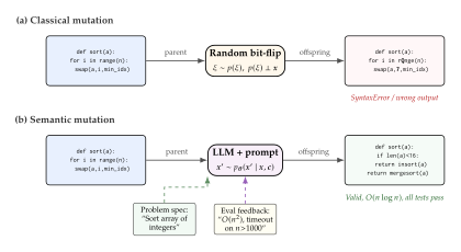
The LLM-Evolutionary Loop
The integration of LLMs into evolutionary search produces a characteristic feedback loop that differs fundamentally from both pure LLM inference and pure evolutionary optimisation. In pure LLM inference, the model generates a single response (or a small number of candidates via temperature sampling) and the process terminates. In pure evolutionary search, a population evolves over many generations under selection pressure but with blind variation. The LLM-evolutionary loop combines the generative power of language models with the sustained exploration and selection pressure of evolutionary computation.
The loop proceeds as follows:
Generate. The LLM generates one or more candidate solutions (or modifications to existing solutions) conditioned on the current population, problem description, and evaluation feedback.
Evaluate. Each candidate is executed in a sandboxed environment and scored against the objective function. This step grounds the LLM's output in reality: no matter how plausible a candidate looks, only its actual performance matters.
Reflect. The evaluation results, including execution traces, error messages, performance metrics, and comparison with the current best solutions, are compiled into a natural-language reflection that explains what worked, what failed, and why.
Mutate. The LLM receives the reflection along with selected parent solutions and generates new candidates that attempt to fix the identified failures, combine the strengths of multiple parents, or explore entirely new approaches suggested by the analysis.
Algorithm 1 (LLM-Guided Evolutionary Search).
- Input: Problem description ; evaluation function ; LLM ; population size ; number of generations ; number of offspring per generation
- Output: Best solution found during search
- Initialise: Generate initial population by prompting with
- Evaluate all solutions: for
- for
- for
- Select parents: Choose from via tournament selection
- Compile context:
- Generate offspring:
- Evaluate:
- Reflect: Natural-language analysis
- Select:
- Update reflection memory with generation results
- return
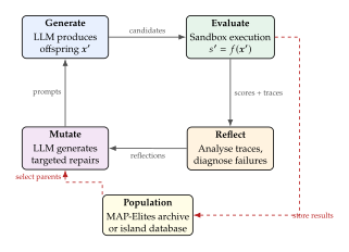
Why the loop matters.
A single LLM inference produces a candidate whose quality is bounded by the model's training distribution and prompt quality. The evolutionary loop transcends this bound in two crucial ways. First, iterative refinement: each generation builds on the accumulated evaluations and reflections of all previous generations, creating an ever-richer context for the LLM. Second, population diversity: maintaining a population of diverse solutions prevents premature convergence to a single local optimum and enables the LLM to combine ideas from multiple high-performing but structurally different solutions. The evolutionary pressure acts as a ratchet that retains improvements while the LLM's semantic understanding guides the search toward promising regions of the solution space.
Semantic Gradients: Natural Language as Optimisation Signal
In classical optimisation, the gradient provides a local linear approximation of the objective function, telling us which direction to move in parameter space to improve the objective most rapidly. In gradient-free evolutionary search, we lose this directional information entirely: we know that mutation produced a fitness of 0.73 and mutation produced a fitness of 0.81, but we have no structured information about why was better or how to improve further.
The introduction of LLMs creates a qualitatively new kind of optimisation signal that we call the semantic gradient. Instead of receiving a scalar fitness value, the LLM-evolutionary system constructs a rich natural-language description of the evaluation outcome: execution traces, error messages, performance profiles, comparison with other solutions, and an explicit analysis of which components of the solution contributed positively or negatively to the overall score.
Definition 30 (Semantic Gradient).
Let be a candidate solution, its scalar fitness, and the evaluation trace consisting of the execution log, error messages, intermediate outputs, timing data, and any other structured feedback from the evaluator. The semantic gradient is a natural-language description (Semantic Gradient) where is either an LLM-generated analysis or a deterministic summariser, is the current population (providing comparison context), and is the set of all natural-language strings. The semantic gradient contains directional information: it identifies which components of should be modified, how they should be modified, and why those modifications are expected to improve fitness.
The semantic gradient is not a gradient in the formal mathematical sense (it does not live in a vector space, and there is no notion of linearity), but it serves the same functional role: it provides directional guidance for the next step of optimisation. The analogy is precise enough to be useful.
Example 10 (Semantic gradient for algorithm optimisation).
Consider evolving a sorting algorithm. A classical evolutionary system might report: “Fitness: 0.67 (correctly sorts 67% of test cases).” A semantic gradient would instead report:
“The algorithm correctly sorts arrays of length but fails on longer arrays. The failure mode is an off-by-one error in the merge step at line 14: the condition
i < len(left)should bei <= len(left). Additionally, the algorithm has complexity on already-sorted inputs because the pivot selection in the partition step always chooses the first element. Consider median-of-three pivot selection to improve average-case performance. The best solution in the current population uses a hybrid approach (insertion sort for small subarrays) that achieves fitness 0.94.”
This semantic gradient identifies the specific bug (off-by-one error), its location (line 14), the performance bottleneck (pivot selection strategy), and a suggestion drawn from the population (hybrid approach).
Key Idea.
From “learning that” to “learning why.” Classical evolutionary search operates on the principle of learning that: it learns that certain solutions have higher fitness than others, and selection pressure gradually accumulates beneficial traits. LLM-guided evolutionary search operates on the principle of learning why: the semantic gradient explains why a solution succeeds or fails, enabling the LLM to generate targeted fixes rather than random perturbations. This shift from correlation-based to explanation-based optimisation is what enables LLM-evolutionary systems to solve problems in hundreds of generations that would require millions of generations under classical blind search.
Formal connection to information-theoretic search.
The semantic gradient can be understood through the lens of information theory. Let denote the entropy of the optimal solution conditioned on the information available at generation . Each evaluation provides information that reduces this entropy. A scalar fitness value provides at most bits of information, where is the discretised fitness range. A semantic gradient , by contrast, can provide information about the structure and location of defects within the solution, potentially yielding bits of information where is the solution length. Formally:
(Semantic Information)
where denotes mutual information. The inequality states that the semantic gradient is at least as informative as the scalar fitness, and in practice is typically far more informative.
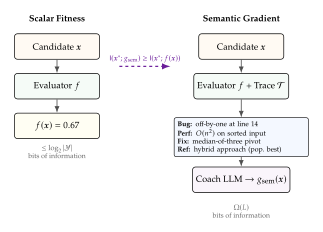
The LLM as Crossover Operator
The semantic variation paradigm extends naturally to crossover. Classical crossover operators (single-point, two-point, uniform) combine genetic material from two parents by selecting crossover points and swapping segments. In structured domains, this frequently produces offspring that are syntactically or semantically broken because the swapped segments are incompatible (e.g., variables referenced in one segment are defined in the other).
An LLM-based crossover operator receives two parent solutions along with their evaluation summaries and is prompted to combine the best aspects of both. The LLM understands the semantic content of each parent and can perform intelligent recombination: taking the data structure from parent and the algorithm from parent , resolving variable name conflicts, adapting interfaces, and producing a coherent offspring that genuinely integrates the strengths of both parents.
Definition 31 (Semantic Crossover).
A semantic crossover operator is a stochastic map that, given two parent solutions and context containing evaluation feedback and problem description, produces an offspring by sampling from: (Semantic Crossover) Unlike classical crossover, the LLM can identify the semantically meaningful components of each parent and recombine them coherently, resolving interface mismatches and preserving invariants.
Prompt engineering for crossover.
A typical crossover prompt might read:
“Below are two solutions to [problem description]. Solution A achieves [score A] with strength [analysis A]. Solution B achieves [score B] with strength [analysis B]. Create a new solution that combines the best aspects of both. Specifically, try to use A's [identified strength] with B's [identified strength]. The solution must be a complete, self-contained program.”
The prompt structure ensures that the LLM's output is both semantically informed (it knows what each parent does well) and practically grounded (it must produce a complete, runnable program).
Connection to Generative Models and Diffusion
The use of LLMs as variation operators creates a beautiful conceptual bridge between evolutionary computation and the generative modelling frameworks we studied in earlier chapters. In diffusion models (19), we learn a denoising process that iteratively transforms random noise into structured samples from a target distribution. In LLM-guided evolution, the LLM plays an analogous role: it transforms a “noisy” solution (one with bugs, inefficiencies, or suboptimal design choices) into a “cleaner” solution that better fits the objective.
The parallel extends further. Classifier-free guidance in diffusion models conditions the denoising process on a desired property (e.g., a text prompt), biasing generation toward samples that satisfy the condition. In LLM-guided evolution, the semantic gradient plays the role of the classifier signal, biasing the LLM's mutations toward solutions that address identified weaknesses. We can formalise this analogy:
(Diffusion Analogy)
where the current (imperfect) solution corresponds to the noisy sample , the improved solution corresponds to the denoised sample , and the semantic gradient corresponds to the conditioning signal .
Remark 13 (Evolutionary search as iterative refinement).
This analogy suggests that LLM-guided evolutionary search can be understood as an iterative refinement process in program space, analogous to the iterative refinement of images in diffusion models. Just as diffusion models require many denoising steps to produce high-quality images from pure noise, LLM-guided evolution requires many generations to refine initial crude solutions into sophisticated, optimised programs. The key insight is that each “denoising step” (generation of evolution) is guided by semantic understanding rather than a learned score function.
Historical Context and Rapid Progress
Historical Note.
From FunSearch to AlphaEvolve: two years that changed everything. The idea of using neural networks to guide evolutionary search predates LLMs by decades: neural network-based surrogate models have been used in evolutionary optimisation since the 1990s [17], and learned crossover operators appeared in the genetic programming literature as early as 2000. But the scale and capability of modern LLMs transformed the idea from a modest improvement into a paradigm shift.
The watershed moment came in December 2023, when DeepMind's FunSearch [11] demonstrated that an LLM (a variant of PaLM 2) could be embedded in an evolutionary loop to discover new mathematical results, specifically new constructions for the cap set problem in extremal combinatorics that surpassed the best known human-designed solutions. FunSearch evolved single Python functions, using an island-based evolutionary model with the LLM as the sole variation operator.
In May 2025, DeepMind unveiled AlphaEvolve [18], which extended the paradigm in several crucial directions: multi-file codebase evolution (not just single functions), a tiered model approach using both fast and powerful LLMs, MAP-Elites quality-diversity archives, and a sophisticated prompt sampling system. AlphaEvolve produced results that astonished the mathematical community, including a new algorithm for complex matrix multiplication using only 48 scalar multiplications, breaking a barrier that had stood since Strassen's 1969 discovery.
The progression from FunSearch to AlphaEvolve in under two years illustrates the explosive pace of progress in this field.
Dangers and Failure Modes
Caution.
LLM hallucinations in evolutionary search. The power of semantic variation operators comes with a corresponding risk. LLMs can and do hallucinate: they generate code that looks correct but contains subtle bugs, mathematical arguments that appear rigorous but contain logical gaps, and optimisation strategies that sound promising but are based on incorrect reasoning.
In a pure LLM inference setting, hallucinations can go undetected. In an evolutionary setting, the evaluation step provides a crucial safeguard: every candidate generated by the LLM is executed, tested, and scored. Hallucinated solutions that do not actually work are assigned low fitness and eliminated by selection. This is the fundamental reason why the LLM-evolutionary loop is more reliable than pure LLM inference: evolution provides a grounding mechanism that filters out the LLM's mistakes.
However, the grounding is only as good as the evaluation function. If the evaluation function is incomplete (e.g., it tests only a few cases), the LLM may evolve solutions that overfit to the test cases while failing on unseen inputs. If the evaluation function has bugs, the evolutionary process may optimise for the wrong objective entirely. Practitioners must invest heavily in evaluation quality to realise the full benefits of LLM-guided evolution.
Exercise 25.
Consider the task of evolving a Python function that computes the -th Fibonacci number. Design a prompt for an LLM-based semantic mutation operator that receives a parent solution (a recursive implementation with exponential time complexity) and its evaluation feedback (correct outputs but timeout on ), and instructs the LLM to generate an improved variant. Your prompt should include: (a) the parent code, (b) the evaluation results, (c) a diagnosis of the performance issue, and (d) specific suggestions for improvement strategies (memoisation, iteration, matrix exponentiation). Discuss why this prompt-based approach is likely to produce a better offspring than random subtree replacement.
Exercise 26.
Prove that for a search space consisting of Python programs of length at most characters, the ratio of syntactically valid programs to all possible character strings is at most . Estimate the constant in the exponent by considering the fraction of random 100-character ASCII strings that parse as valid Python. (Hint: Use the fact that Python requires matching parentheses, colons after control-flow keywords, and consistent indentation.)
Exercise 27.
Design an ablation experiment to measure the contribution of each component of the semantic gradient. Specifically, compare four conditions: (a) scalar fitness only, (b) fitness plus error messages, (c) fitness plus error messages plus execution traces, and (d) full semantic gradient with population comparison and natural-language analysis. For each condition, describe what information the LLM receives and predict which condition will produce the fastest convergence. Justify your predictions using the information-theoretic framework of (Semantic Information).
Exercise 28.
Implement the LLM-evolutionary loop of Algorithm 1 for the task of evolving a function that computes the maximum independent set of a graph. Use a population of , offspring per generation, and run for generations. Use any available LLM API as the variation operator. Report: (a) the fitness trajectory over generations, (b) the survival rate (fraction of offspring that are syntactically and semantically valid), and (c) qualitative examples of the semantic gradients produced by the reflection step.
AlphaEvolve: Open-Ended Algorithmic Discovery
In May 2025, DeepMind published a system that quietly but unmistakably crossed a threshold. AlphaEvolve did not merely optimise existing algorithms or fine-tune known solutions: it discovered new mathematical constructions and engineering optimisations that had eluded human researchers for decades. Among its achievements was a new algorithm for multiplying matrices over the complex numbers using only 48 scalar multiplications, improving upon a record that had stood since Volker Strassen's landmark 1969 paper [19].
What makes AlphaEvolve remarkable is not any single result but the generality of its approach. The same system, with minimal task-specific engineering, produced state-of-the-art results across domains as diverse as combinatorial mathematics, compiler optimisation, chip design, data centre scheduling, and GPU kernel programming. In this section we dissect the architecture and mechanisms that make this generality possible.
Architecture Overview
AlphaEvolve integrates four major components into a coherent system: (1) an evolutionary database that maintains a diverse population of candidate programs, (2) a prompt sampler that constructs rich context from the population, (3) a tiered ensemble of LLMs that generate mutations and new candidates, and (4) an evaluator pool that grounds every candidate in empirical reality through sandboxed execution.
Definition 32 (AlphaEvolve Architecture).
The AlphaEvolve system is a tuple where:
is the evolutionary database, a MAP-Elites archive that maps each behavioural descriptor to a set of candidate programs, organised into islands with periodic migration.
is the prompt sampler, a stochastic procedure that, given the current state of , constructs a prompt by selecting parent programs, inspirations from other islands, evaluation summaries, and task-specific instructions.
is the tiered LLM ensemble, consisting of a fast model (Gemini Flash) used for the majority of mutations and a powerful model (Gemini Pro) reserved for difficult mutations requiring deeper reasoning.
is the evaluator pool, a collection of sandboxed execution environments that compile, run, and score candidate programs against the objective function, returning both scalar fitness and structured evaluation traces.
The system operates in an asynchronous event loop: the prompt sampler continuously extracts parents from , the LLMs generate mutations, and the evaluator pool scores them, with results flowing back into .
The evolutionary database.
The database uses a MAP-Elites architecture (MAP-Elites) extended with an island model [15]. Each island maintains its own MAP-Elites archive, with solutions characterised by behavioural descriptors that capture different aspects of solution quality (e.g., for a sorting algorithm: time complexity class, space usage, and stability). Periodically, the best solutions from each island migrate to other islands, injecting diversity and enabling the cross-pollination of ideas across semi-independent evolutionary lineages.
The island model serves a dual purpose. First, it maintains diversity: different islands may converge to different local optima, and migration allows the best features of each to combine. Second, it provides a natural parallelism structure: each island can evolve independently, with migration events providing synchronisation points.
The prompt sampler.
The prompt sampler is perhaps the most sophisticated component, responsible for constructing the context that guides the LLM's mutations. For each mutation, performs the following steps:
Parent selection. Select one or two parent programs from the evolutionary database using a combination of fitness- proportionate and diversity-based selection.
Inspiration selection. With probability , additionally select a high-performing program from a different island as an “inspiration” that the LLM can draw ideas from without directly combining code.
Context assembly. Combine the parent program(s), their evaluation summaries, the problem description, any EVOLVE-BLOCK markers (described below), and optional inspirations into a structured prompt.
Instruction generation. Append a natural-language instruction that specifies the type of mutation desired: “improve the time complexity,” “fix the bug on edge case ,” “try a completely different algorithmic approach,” or “combine the data structure from parent A with the algorithm from parent B.”
Tiered model allocation.
AlphaEvolve uses two tiers of LLMs: Gemini Flash for approximately 80% of mutations and Gemini Pro for the remaining 20%. The allocation is not random but is guided by the difficulty of the mutation. Simple refinements (fixing syntax errors, adjusting constants, minor restructuring) are handled by the fast model. Fundamental algorithmic redesigns, novel mathematical constructions, and mutations that require deep chain-of-thought reasoning are routed to the powerful model.
This tiered approach reflects a fundamental insight about the structure of evolutionary search: most mutations are incremental refinements that do not require the full reasoning capacity of a frontier model. Allocating expensive compute only to the mutations that need it yields a dramatic improvement in cost-efficiency without sacrificing the quality of breakthrough discoveries.
Algorithm 2 (AlphaEvolve Pipeline).
- Input: Problem specification ; initial codebase with EVOLVE-BLOCK markers; fast LLM ; deep LLM ; number of islands ; migration interval ; evaluation function ; total budget
- Output: Best program
- Initialise islands, each seeded with variants of
- Evaluate all initial candidates and populate MAP-Elites archives
- for Asynchronous event loop
- Select island proportional to recent improvement rate
- Prompt sampler
- Determine difficulty based on mutation type
- if
- Deep model for hard mutations
- else
- Fast model for routine mutations
- Sandbox execution
- if is valid and
- Insert into 's MAP-Elites archive
- if
- Migrate top solutions between islands Cross-pollination
- return
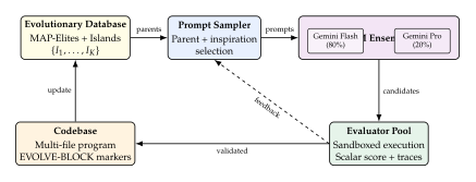
Multi-Block Coevolution
One of AlphaEvolve's most powerful capabilities is its ability to evolve multiple interdependent components of a codebase simultaneously. Classical evolutionary approaches typically evolve a single function or a single configuration file. Real-world optimisation problems, however, often require coordinated changes across multiple components: the search algorithm must co-adapt with the data structure it operates on, the mathematical formula must co-evolve with the numerical method that evaluates it, and the hardware kernel must co-evolve with the scheduling policy that dispatches work to it.
AlphaEvolve enables this through EVOLVE-BLOCK markers: special annotations in the codebase that delineate regions subject to evolutionary modification. A single codebase can contain multiple EVOLVE-BLOCK regions, and the evolutionary process can modify any subset of them in a single mutation.
Definition 33 (Multi-Block Coevolution).
Let a codebase be partitioned into fixed regions and evolvable blocks , where each is delimited by EVOLVE-BLOCK markers. A multi-block coevolutionary mutation is a transformation that modifies a subset of evolvable blocks simultaneously: (Multiblock) where the LLM conditions on the entire codebase (including all blocks) and context . Blocks not in remain unchanged: for .
The joint distribution over modified blocks captures coevolutionary dependencies: the LLM understands that changing block may require compensating changes in block to maintain overall correctness.
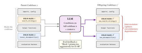
Example 11 (Coevolving search and solution).
Consider the problem of finding optimal matrix multiplication algorithms. The codebase contains two EVOLVE-BLOCK regions:
Block 1 (search algorithm): The procedure that explores the space of bilinear decompositions, including the search strategy, pruning heuristics, and branching rules.
Block 2 (candidate solution): The actual tensor decomposition representing a matrix multiplication algorithm with scalar multiplications.
AlphaEvolve can simultaneously modify the search strategy (Block 1) to focus on a new region of the decomposition space and propose a candidate decomposition (Block 2) tailored to that region. This coevolutionary capability was essential for the breakthrough on complex matrix multiplication: the system needed to co-discover both the right search strategy and the right algebraic structure.
Remark 14 (Coevolution vs. independent evolution).
Multi-block coevolution is strictly more powerful than independent evolution of each block. Independent evolution treats each block as a separate optimisation problem, ignoring the interactions between blocks. Coevolution captures these interactions by evolving blocks jointly, conditioned on the full codebase context. The fitness of the composite solution is generally not decomposable as , and the interactions between blocks (epistatic effects, in genetic terminology) can be decisive.
Landmark Results
AlphaEvolve's results span multiple domains, from pure mathematics to production engineering systems. We review the most significant achievements, each of which illustrates a different aspect of the system's capabilities.
Matrix multiplication: breaking the 56-year barrier.
The problem of multiplying two matrices is one of the most fundamental in computer science. The naive algorithm requires scalar multiplications. In 1969, Volker Strassen showed that two matrices could be multiplied using only 7 scalar multiplications instead of 8, leading to an overall complexity of via recursive decomposition [19]. This was the first demonstration that the cubic barrier could be broken, and it launched an entire field of research into fast matrix multiplication algorithms.
For matrices over the complex numbers , the best known algorithm before AlphaEvolve required 49 scalar multiplications (achieved through a combination of Strassen-like recursive decompositions and computer-assisted search). AlphaEvolve discovered an algorithm using only 48 scalar multiplications, improving a record that had been refined incrementally over more than five decades.
Theorem 5 (AlphaEvolve Matrix Multiplication, 2025).
There exists a bilinear algorithm for multiplying two matrices over using exactly 48 scalar multiplications. Formally, there exist vectors for such that for all : (Matmul 48) where are the coefficients discovered by AlphaEvolve.
The significance of this result extends beyond the specific constant. Matrix multiplication is a fundamental primitive in virtually all of scientific computing, and any improvement in the constant factor or asymptotic complexity has cascading effects across numerical linear algebra, machine learning, signal processing, and physics simulations.
Combinatorial optimisation: broad superiority.
AlphaEvolve was evaluated on over 50 open problems from combinatorial mathematics, including extremal graph theory, coding theory, and combinatorial design. The results were striking: approximately 75% of the time, AlphaEvolve matched the best known human-designed constructions, and on approximately 20% of problems, it surpassed the state of the art, discovering constructions that no human had found [18].
Borg scheduler optimisation.
Google's Borg cluster management system schedules jobs across millions of machines in data centres worldwide. AlphaEvolve was applied to optimise the scheduling heuristics in Borg, evolving the scoring functions that determine how jobs are assigned to machines. The result was a 0.7% improvement in overall resource recovery, which translates to recovering approximately 0.7% of all compute resources across Google's worldwide infrastructure. Given the enormous scale of this infrastructure, even a fraction-of-a-percent improvement represents hundreds of millions of dollars in annual value.
FlashAttention kernel optimisation.
FlashAttention [41] is a memory-efficient implementation of the attention mechanism that has become a critical component of modern transformer training. AlphaEvolve evolved optimised GPU kernels for FlashAttention, achieving a 32.5% speedup over the existing hand-tuned implementation. This is particularly remarkable because FlashAttention was already heavily optimised by expert GPU programmers; the fact that an automated system could find a significant further improvement suggests that the space of possible kernel optimisations is far larger than human engineers can explore manually.
TPU Verilog optimisation.
AlphaEvolve was also applied to optimise the Verilog hardware description language code for Google's Tensor Processing Units (TPUs). The system evolved circuit-level optimisations in the matrix multiply unit, achieving improvements in area and timing that were deployed in production TPU designs. This application demonstrates the system's ability to operate at the hardware level, evolving low-level circuit descriptions that require deep understanding of digital logic, timing constraints, and power dissipation.
| Domain | Problem | Previous best | AlphaEvolve |
| Mathematics | complex matmul | 49 mults | 48 mults |
| Mathematics | Cap set constructions | Human-designed | New records |
| Combinatorics | 50+ open problems | State of art | 20% improved |
| Systems | Borg scheduler | Production baseline | +0.7% recovery |
| ML kernels | FlashAttention | Hand-tuned | +32.5% speedup |
| Hardware | TPU Verilog | Engineer-designed | Area + timing gains |
| Algorithms | Sorting networks | Known optimal | Matched or improved |
Insight.
AI as mathematical discoverer. The AlphaEvolve results on matrix multiplication and combinatorial optimisation represent something qualitatively new in the history of mathematics. For the first time, an automated system has discovered mathematical constructions that are provably correct (verified by symbolic computation) and genuinely novel (not previously known to human mathematicians). This is not AI replacing mathematicians but AI expanding the frontier of what is mathematically known. The constructions discovered by AlphaEvolve are now part of the mathematical literature, cited and studied by human researchers who seek to understand the structures that the system found but could not explain.
This raises a profound epistemological question: can we be said to understand a mathematical result that was discovered by a machine? The AlphaEvolve constructions are verifiable (we can check that 48 multiplications suffice) but not yet explainable (we do not have a human-comprehensible proof of why 48 suffice or whether 47 might also work). The gap between verification and explanation is one of the central philosophical challenges posed by AI-driven discovery.
Historical Note.
Strassen's algorithm and the 56-year barrier. When Volker Strassen published his algorithm for matrix multiplication using 7 multiplications in 1969 [19], it overturned a widely held belief that multiplications were necessary. Strassen's insight was to express the product of two matrices using seven carefully chosen intermediate products: The entries of the product are then recovered as: , , , and .
The recursive application of this decomposition yields complexity. Subsequent work reduced the exponent further: Coppersmith and Winograd achieved in 1987, and the current best bound is due to Alman and Vassilevska Williams (2024). For fixed small sizes, the problem of finding the minimal number of scalar multiplications remained challenging: the 49-multiplication barrier for complex matrices stood for decades until AlphaEvolve's 48-multiplication algorithm in 2025.
Evaluation and Grounding
The evaluation pool is the component that transforms LLM-guided evolution from speculative generation into grounded discovery. Every candidate program produced by the LLM is compiled and executed in a sandboxed environment with strict resource limits (CPU time, memory, disk space). The evaluator produces two outputs:
A scalar fitness that summarises the candidate's quality.
An evaluation trace that includes compilation output, runtime logs, intermediate values, timing measurements, test case results, and any error messages.
The scalar fitness determines whether the candidate enters the evolutionary database. The evaluation trace feeds back into the prompt sampler to construct semantic gradients for future mutations.
Lemma 2 (Grounding eliminates hallucinated improvements).
Let be a candidate generated by the LLM and let be the LLM's predicted fitness (implicit in its generation process). Let be the actual fitness measured by the evaluator. If the evaluator is faithful (i.e., correctly measures the true objective), then the evolutionary database contains only candidates with verified fitness: (Grounding) In particular, LLM hallucinations that produce candidates with (solutions that the LLM “believes” are good but actually are not) are filtered out by evaluation and never enter the database.
Proof.
By construction, a candidate enters only after evaluation by , which computes by executing . The stored fitness is , not any estimate derived from the LLM. Therefore, every entry in has verified fitness, and hallucinated improvements are eliminated by the evaluation step.
Multi-objective evaluation.
For many problems, the evaluation function is multi-objective. For example, when optimising a GPU kernel, AlphaEvolve evaluates both throughput (operations per second) and numerical accuracy (error relative to a reference implementation). The MAP-Elites archive naturally accommodates multi-objective evaluation by using the different objectives as behavioural descriptors, maintaining solutions that are Pareto-optimal across the objective space.
Exercise 29.
Consider applying AlphaEvolve to optimise a Python implementation of quicksort. Define: (a) appropriate EVOLVE-BLOCK markers for the partition function, the pivot selection strategy, and the base case threshold; (b) a multi-objective evaluation function that measures both running time and number of comparisons; (c) behavioural descriptors for a MAP-Elites archive that would encourage diversity across different algorithmic strategies (e.g., randomised vs. deterministic pivot selection, in-place vs. out-of-place partitioning).
Exercise 30.
The bilinear decomposition in (Matmul 48) can be verified by symbolic computation. Write a verification algorithm that, given vectors for , checks whether the decomposition correctly computes all entries of the matrix product for symbolic matrices . Analyse the computational complexity of your verification algorithm as a function of and .
Exercise 31.
Design a migration strategy for AlphaEvolve's island model that balances exploration and exploitation. Specifically: (a) define a migration topology (which islands can exchange solutions with which others), (b) define a migration selection criterion (which solutions migrate), and (c) define a migration replacement criterion (which solutions in the receiving island are replaced). Prove that your strategy preserves the best solution found so far (elitism) while guaranteeing that every island eventually receives genetic material from every other island (ergodicity).
Exercise 32.
Suppose AlphaEvolve uses Gemini Flash at cost per query and Gemini Pro at cost per query, with . If the system allocates fraction of mutations to the deep model, derive the total cost as a function of and the total number of mutations . If the probability of a breakthrough discovery per deep-model mutation is and per fast-model mutation is , find the value of that maximises the expected number of breakthroughs per unit cost.
The Open-Source Ecosystem: OpenEvolve and CodeEvolve
The publication of AlphaEvolve's architecture and results catalysed a rapid open-source response. Within weeks of the original paper, independent teams released open-source implementations that replicated the core LLM-evolutionary loop, adapted it for different use cases, and introduced novel algorithmic innovations. This section surveys the three most significant open-source systems – OpenEvolve, CodeEvolve, and LEVI – and analyses how they extend, simplify, or improve upon the original AlphaEvolve design.
The existence of this ecosystem is itself significant. Unlike many industrial AI systems that remain proprietary and irreproducible, the LLM-evolutionary paradigm is inherently reproducible: the core algorithm (Algorithm 1) is straightforward to implement, and the variation operator is any LLM accessible via API. This accessibility has enabled a Cambrian explosion of experimentation by researchers, hobbyists, and small teams who lack the resources of a major AI lab but possess domain expertise in specific optimisation problems.
OpenEvolve: Democratising LLM-Evolutionary Search
OpenEvolve [42] is an open-source implementation of the LLM-evolutionary search paradigm designed for maximum generality and accessibility. Its architecture closely follows the AlphaEvolve blueprint but makes several pragmatic adaptations for the open-source setting: support for any LLM API (not just Gemini), multi-language evaluation support, simplified configuration, and extensive logging for reproducibility.
Architecture.
OpenEvolve consists of four modules that mirror the AlphaEvolve components:
Population Manager. Maintains the evolutionary population using a simplified island model with islands (default ). Each island stores candidates as pairs of program text and scalar fitness, ranked by fitness within each island. Migration occurs every generations by copying the best candidate from each island to a randomly selected neighbour.
Prompt Engine. Constructs prompts for the LLM by selecting one or two parents from the current island, formatting them with evaluation feedback and problem description, and appending a mutation instruction. The prompt engine supports customisable templates that can be adapted to different problem domains.
LLM Interface. A generic API layer that supports OpenAI-compatible APIs, Anthropic Claude, Google Gemini, and local models via Ollama or vLLM. This abstraction allows users to swap LLMs without modifying any other component.
Evaluation Harness. A sandboxed execution environment that supports Python, Rust, R, C++, and Metal shader programs. Each candidate is executed with configurable timeouts and resource limits. The evaluation harness returns both a scalar score and structured feedback (stdout, stderr, timing data, test results).
Algorithm 3 (OpenEvolve Pipeline).
- Input: Problem specification ; evaluation script ; LLM API endpoint ; number of islands ; population size per island ; generations ; migration interval
- Output: Best program
- Seed: For each island : generate initial candidates using with varied temperature
- Evaluate all candidates: for all
- for
- for each island in parallel
- Select parent via tournament selection (tournament size 3)
- Compile prompt:
- Generate offspring:
- Evaluate:
- if
- Replace worst candidate in island with
- Log: generation , island , parent score , offspring score
- if
- Migrate: For each island , copy best candidate to island
- return
Multi-language support.
A distinguishing feature of OpenEvolve is its support for evolving programs in multiple programming languages. The evaluation harness includes language-specific runners for:
Python: Direct execution with
subprocess, supporting NumPy, SciPy, and PyTorch imports.Rust: Compilation with
rustcfollowed by execution, enabling evolution of high-performance systems code.R: Execution via
Rscript, targeting statistical computing and data analysis applications.Metal shaders: Compilation and execution on Apple GPUs via the Metal Performance Shaders framework, enabling evolution of GPU compute kernels for Apple hardware.
This multi-language capability reflects the insight that different optimisation problems are most naturally expressed in different languages: numerical algorithms in Python, systems code in Rust, statistical models in R, and GPU kernels in Metal or CUDA.
Results.
OpenEvolve has been applied to a diverse set of problems by the open-source community, with notable results including:
Circle packing: Evolving algorithms for packing circles of varying radii into a square container, achieving packing densities competitive with specialised mathematical solvers.
FIR filter design: Evolving finite impulse response filter coefficients for signal processing applications, discovering filters with better stopband attenuation than Parks-McClellan designs for certain specifications.
MLX kernels: Evolving optimised compute kernels for Apple's MLX machine learning framework, achieving speedups of 15–25% over the default implementations for matrix operations on M-series chips.
Remark 15 (The power of varied temperature).
OpenEvolve assigns different sampling temperatures to different islands: island 1 uses (conservative, exploitative mutations), while island 5 uses (creative, exploratory mutations). This temperature-based diversity mechanism is simple but effective. Low-temperature islands produce reliable incremental improvements that steadily climb the fitness landscape. High-temperature islands produce wild, often-failing mutations that occasionally discover entirely new approaches. Migration carries the best discoveries from high-temperature islands to low-temperature islands, where they are refined and polished. This division of labour between exploration and exploitation emerges naturally from the island model without any explicit mechanism for controlling the exploration-exploitation trade-off.
CodeEvolve: Meta-Prompting and Transparent Evaluation
CodeEvolve [43] introduces two innovations that distinguish it from both AlphaEvolve and OpenEvolve: meta-prompting, in which the LLM evolves its own mutation instructions, and transparent evaluation, in which the full evaluation pipeline is visible to and modifiable by the user.
Meta-prompting: evolving the evolution strategy.
In standard LLM-evolutionary search, the prompt template that instructs the LLM how to mutate solutions is fixed by the system designer. CodeEvolve recognises that the prompt template is itself a crucial design choice that significantly affects the quality and diversity of mutations. Rather than fixing the template, CodeEvolve treats it as an additional evolvable component.
Definition 34 (Meta-Prompting in Evolutionary Search).
Let be the space of prompt templates and the space of candidate solutions. A meta-prompting evolutionary system maintains a population of template-solution pairs where is the prompt template used to generate . Evolution operates on two levels:
Solution level: Given template and parent , the LLM generates an offspring solution: (META Solution)
Template level: The LLM generates a modified template: (META Template) where is a meta-instruction asking the LLM to “improve the mutation prompt based on which types of mutations have been most successful so far.”
The fitness of a template-solution pair is the solution fitness . Selection operates on the joint population, simultaneously selecting for both good solutions and the templates that produced them.
The meta-prompting mechanism enables the system to adapt its mutation strategy to the problem at hand. For example, if the system discovers that mutations focused on “simplifying the algorithm” tend to produce higher-fitness offspring than mutations focused on “adding features,” the template population will shift toward simplification-oriented prompts. This is a form of self-adaptation, analogous to the self-adaptive mutation step sizes in evolution strategies (Evolution Strategies).
Example 12 (Meta-prompt evolution in practice).
Consider evolving a sorting algorithm. The initial prompt template might read: “Improve the following sorting algorithm. Focus on reducing time complexity.” After several generations, the meta-prompting mechanism might evolve this template to: “The parent algorithm uses comparison-based sorting with average case. Try a non-comparison-based approach (radix sort, counting sort) if the input domain is bounded. Alternatively, optimise the inner loop by reducing branch mispredictions. Look at the execution trace to identify the hottest loop.”
The evolved template is more specific, more informed by the problem structure, and more likely to produce useful mutations. The meta-prompting mechanism discovers this template through the same evolutionary process that discovers good solutions.
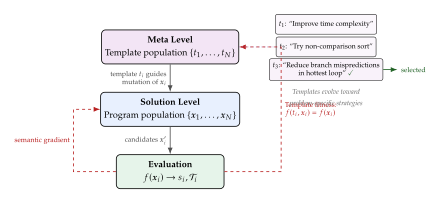
Elitist migration.
CodeEvolve implements a migration strategy between islands that is strictly elitist: only solutions that represent a Pareto improvement over any existing solution in the destination island are accepted. This prevents the dilution of high-quality island populations by mediocre migrants, a problem that can occur with the unconditional migration used in simpler island models.
Formally, let be the set of fitness values in island , and let be a candidate migrant with fitness . The migrant is accepted into island only if: (Elitist Migration) where the second condition prevents the introduction of near-duplicates that would reduce diversity without improving fitness. The distance function is typically edit distance between program texts or a semantic similarity metric based on output behaviour.
Transparent evaluation.
CodeEvolve makes the evaluation pipeline a first-class citizen of the system: the evaluation script is written in plain Python, included in the project repository, and fully visible to the user. The user can modify the evaluation function at any time during the evolutionary run, enabling interactive refinement of the fitness landscape. This transparency is essential for trust: the user can inspect exactly how fitness is computed, verify that the evaluation is correct, and adjust it when the evolutionary process converges to an unexpected local optimum that exploits an evaluation loophole.
LEVI: Stratified Model Allocation
LEVI (LLM-Evolutionary Variation with Intelligence stratification) [44] focuses on a problem that becomes critical as LLM-evolutionary search scales: the cost of frontier model queries. A single query to a state-of-the-art model like GPT-4 or Claude Opus can cost 10–100 more than a query to a smaller model like GPT-4o-mini or Claude Haiku. If every mutation in a population of thousands over hundreds of generations requires a frontier model query, the total cost becomes prohibitive for most research groups.
LEVI addresses this with a stratified model allocation strategy that assigns different tiers of LLMs to different types of mutations based on their expected difficulty and importance.
The stratification principle.
LEVI classifies mutations into three tiers:
Tier 1: Routine refinements (80–90% of mutations). These include constant tweaking, minor refactoring, adding edge case handling, and fixing obvious bugs. These mutations are well within the capability of small, inexpensive models and are assigned to the cheapest available LLM (e.g., GPT-4o-mini, Claude Haiku, Gemini Flash).
Tier 2: Structural modifications (8–15% of mutations). These include changing data structures, modifying algorithmic flow, adding new subroutines, and combining ideas from multiple parents. These require moderate reasoning capability and are assigned to a mid-tier model (e.g., Claude Sonnet, GPT-4o).
Tier 3: Paradigm shifts (2–5% of mutations). These are attempts at fundamental algorithmic redesign: replacing a greedy algorithm with dynamic programming, switching from iterative to recursive approaches, or introducing entirely new mathematical constructions. These require the deepest reasoning and are assigned to a frontier model (e.g., Claude Opus, GPT-4, Gemini Ultra).
Proposition 14 (Cost-Efficiency of Stratified Allocation).
Let be the per-query costs of the three model tiers, and let , , be the expected quality of mutations at each tier, where is the fraction of mutations allocated to tier with . Under the assumption that quality increases with model capability but with diminishing returns for routine mutations (i.e., but ), the stratified allocation achieves at least 90% of the quality of uniform frontier-model allocation at approximately to the cost: (Stratified COST) With typical pricing ratios , , this yields , a cost reduction.
Proof.
The total cost under stratified allocation for mutations is (Stratified Proof) The uniform cost is , giving the ratio , which rounds to a reduction.
For quality, the key observation is that Tier 1 mutations (routine refinements) produce nearly identical results regardless of model size, because they involve straightforward edits within the LLM's competence at all scales. The quality loss from using cheap models for Tier 1 is therefore negligible. Tier 3 mutations genuinely benefit from frontier models, but they constitute only 5% of all mutations, so allocating frontier models to this small fraction is sufficient to capture the quality benefit.
Key Idea.
Not every mutation needs a frontier model. The stratified allocation principle reflects a deep truth about the structure of evolutionary search: the vast majority of mutations are incremental refinements that any competent model can perform. The rare, high-value mutations that require deep reasoning and creative insight constitute a tiny fraction of the total. By matching model capability to mutation difficulty, we achieve nearly the same search quality at a fraction of the cost. This principle applies not only to LLM-evolutionary search but to any system that uses LLMs for repetitive tasks with varying difficulty levels.
Tier classification.
LEVI classifies mutations into tiers using a combination of heuristics and learned classifiers:
Edit distance heuristic. If the requested mutation involves changes to fewer than 5 lines of code, it is classified as Tier 1. If it involves 5–30 lines, Tier 2. If it involves more than 30 lines or requires generating entirely new code, Tier 3.
Prompt complexity. The mutation prompt is analysed for keywords indicating difficulty: “fix bug,” “adjust constant,” “improve readability” suggest Tier 1; “restructure,” “add caching,” “change data structure” suggest Tier 2; “redesign algorithm,” “try a completely different approach,” “novel mathematical construction” suggest Tier 3.
Stagnation detection. If the population has not improved for consecutive generations, the system increases the fraction of Tier 3 mutations, reasoning that incremental refinements have been exhausted and a paradigm shift is needed.
Adaptive tier allocation.
LEVI does not fix the tier fractions but adapts them based on the improvement rate at each tier. Let be the fraction of tier- mutations that produce offspring fitter than their parents. LEVI updates the allocation using a softmax rule: (Adaptive Allocation) where is a temperature parameter that controls the sharpness of the allocation. The ratio measures the improvement per unit cost at each tier, ensuring that the system allocates resources to the tier that provides the best return on investment.
Comparative Analysis
The four systems – AlphaEvolve, OpenEvolve, CodeEvolve, and LEVI – represent different points in the design space of LLM-evolutionary search. Table 7 summarises their key architectural choices and capabilities.
| Feature | AlphaEvolve | OpenEvolve | CodeEvolve | LEVI |
| Developer | DeepMind | Community | Community | Community |
| LLM support | Gemini only | Any API | Any API | Any API |
| Population model | MAP-Elites + islands | Islands | Islands | Islands |
| Multi-block coevol. | Yes | Partial | No | No |
| Meta-prompting | No | No | Yes | No |
| Tiered models | 2-tier | Single | Single | 3-tier |
| Languages | Python, C++ | Py, Rust, R, Metal | Python | Python |
| Open source | No | Yes | Yes | Yes |
Architectural trade-offs.
Each system makes different trade-offs between complexity and capability:
AlphaEvolve is the most sophisticated system, with multi-block coevolution, MAP-Elites quality-diversity archives, and a highly engineered prompt sampler. Its complexity is justified by the scale and importance of its target problems (production systems at Google), but makes it difficult to reproduce or adapt for different settings.
OpenEvolve prioritises accessibility and generality. Its simpler architecture (basic island model, single LLM tier) makes it easy to set up and use, and its multi-language support enables a wide range of applications. The trade-off is that it may not achieve the same peak performance as AlphaEvolve on the hardest problems.
CodeEvolve introduces meta-prompting, which adds a new dimension of adaptivity but also increases the search space (the system must search over both solutions and prompts). Transparent evaluation provides an important trust and debugging benefit. The trade-off is increased complexity in the evolutionary dynamics.
LEVI focuses on cost-efficiency through stratified model allocation. Its key contribution is demonstrating that near-frontier quality can be achieved at a fraction of the cost by matching model capability to mutation difficulty. The trade-off is the overhead of tier classification and adaptive allocation.
Island Model Topologies
The island model is a common architectural element across all four systems. The migration topology, which determines which islands can exchange solutions with which others, has a significant effect on the balance between exploration and exploitation. We examine several topologies and their properties.
Definition 35 (Migration Topology).
A migration topology for islands is a directed graph where an edge indicates that solutions from island can migrate to island . The migration diameter is the length of the longest shortest path in , representing the maximum number of migration events needed for a solution to travel from any island to any other.
Common topologies include:
Ring topology. Each island sends migrants to its clockwise neighbour. Migration diameter: . This topology provides slow but steady mixing, giving each island time to develop its own evolutionary trajectory before being influenced by distant islands.
Fully connected. Every island can send migrants to every other island. Migration diameter: 1. This provides the fastest mixing but reduces the independence of islands, potentially causing premature convergence.
Star topology. One central island receives migrants from all others and sends migrants to all others. Peripheral islands do not communicate directly. Migration diameter: 2. This creates a “melting pot” in the central island while preserving diversity in the periphery.
Random sparse graph. Each island has randomly chosen neighbours with . Migration diameter: . This provides a good balance between mixing speed and island independence.
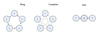
Proposition 15 (Mixing Time and Convergence).
Let be the migration topology with adjacency matrix and let be the row-normalised transition matrix where is the degree matrix. The mixing time of the migration process is (Mixing TIME) where is the second-largest eigenvalue of in absolute value. For a ring of islands: (Mixing RING) while for a complete graph: (Mixing Complete)
Proof.
For the ring graph on vertices, the eigenvalues of the normalised transition matrix are for . The second-largest eigenvalue is , giving spectral gap and mixing time .
For the complete graph, for all , giving spectral gap and mixing time .
Remark 16 (Topology selection in practice).
The optimal migration topology depends on the problem structure. Problems with many distinct local optima benefit from slow-mixing topologies (ring or sparse graphs) that allow each island to explore its local optimum thoroughly before mixing. Problems with a single global basin of attraction benefit from fast-mixing topologies (complete or star) that quickly propagate improvements across all islands. In practice, most systems default to the ring topology as a reasonable compromise.
Challenges and Future Directions
The open-source ecosystem faces several challenges that are active areas of research and development.
Evaluation bottleneck.
The evaluation step is typically the computational bottleneck in LLM-evolutionary search. While LLM queries take seconds, program evaluation can take minutes (for numerical simulations), hours (for training neural networks), or days (for hardware synthesis). Surrogate models that predict fitness from program features can alleviate this bottleneck but introduce approximation errors that may mislead the evolutionary process.
Definition 36 (Surrogate-Assisted LLM Evolution).
A surrogate-assisted LLM-evolutionary system maintains a learned surrogate model that approximates the true evaluation function . Candidates are first screened by the surrogate: (Surrogate) This reduces the number of expensive true evaluations while maintaining the grounding property: only candidates that pass the true evaluation enter the evolutionary database.
Prompt sensitivity.
The quality of LLM-generated mutations is highly sensitive to the prompt format, wording, and structure. Small changes in the prompt template can dramatically alter the distribution of generated mutations. CodeEvolve's meta-prompting addresses this by evolving the prompts themselves, but a principled understanding of what makes a good evolutionary prompt remains an open question.
Reproducibility.
LLM-evolutionary search is inherently stochastic at two levels: the LLM's sampling process and the evolutionary selection process. Reproducing results requires fixing both the LLM (including exact version and API parameters) and the random seeds for selection. Because LLM providers frequently update their models, exact reproduction of published results may be impossible even with identical code and configuration. OpenEvolve addresses this partially through extensive logging and the option to use local models via Ollama.
Scaling laws.
It remains unclear how the performance of LLM-evolutionary search scales with population size, number of generations, and model size. Empirical evidence from AlphaEvolve suggests that performance improves consistently with compute budget, but whether this scaling follows a power law (analogous to neural scaling laws) or has diminishing returns is an open question.
Exercise 33.
Implement the OpenEvolve pipeline (Algorithm 3) for the task of evolving a Python function that computes the edit distance between two strings. Use islands with temperatures , a population of per island, and generations. Compare the results using three different LLMs (e.g., GPT-4o-mini, Claude Haiku, and Gemini Flash) as the variation operator. Report: (a) convergence speed, (b) final solution quality (correctness and efficiency), and (c) cost per generation for each LLM.
Exercise 34.
Design a meta-prompting experiment following Definition 34. Start with three initial prompt templates of varying specificity (generic, moderately specific, and highly specific). Run the system for 50 generations on a problem of your choice and track: (a) the evolution of the prompt templates over generations, (b) the fitness of solutions produced by each template family, and (c) whether the evolved templates converge to a common style or maintain diversity.
Exercise 35.
Derive the optimal stratified allocation that maximises the expected total improvement subject to the budget constraint and , . Solve this as a linear program and interpret the dual variables. Under what conditions does the optimal allocation assign (i.e., never use the frontier model)?
Exercise 36.
For an island model with islands arranged in a ring topology, compute the mixing time using Proposition 15. Then modify the topology by adding a single “shortcut” edge between islands 1 and 5. Recompute the mixing time and show that this small-world modification reduces the mixing time from to .
Exercise 37.
Implement the adaptive tier allocation rule of (Adaptive Allocation). Simulate an evolutionary run where Tier 1 mutations have improvement rate , Tier 2 has , and Tier 3 has , with costs , , . Plot the tier allocation fractions as a function of generation number for temperature values . Discuss how affects the allocation dynamics.
Exercise 38.
Compare the ring, complete, and star migration topologies on a multi-modal optimisation benchmark (e.g., Rastrigin's function in 10 dimensions). For each topology, run an island model with islands, individuals per island, and migration every generations. Report: (a) the number of distinct local optima found by each topology, (b) the best fitness achieved, and (c) the generation at which the globally best solution first appears. Explain your results in terms of the mixing time analysis of Proposition 15.
Synthesis: The New Evolutionary Paradigm
Let us step back and consider what this section and the preceding one have established. The fusion of large language models with evolutionary computation represents a genuine paradigm shift in optimisation, one that combines the sustained exploration and selection pressure of evolution with the semantic understanding and generative power of modern AI.
The classical evolutionary algorithm explores by blind variation and selects by survival of the fittest. The LLM-evolutionary algorithm explores by intelligent variation, mutation that understands what it is mutating and why, and selects by grounded evaluation that verifies every candidate in the real world. The result is a search process that is orders of magnitude more efficient than classical evolution on structured domains.
Several principles have emerged from the systems we have studied:
Semantic variation is the key innovation. The replacement of blind random mutation with LLM-guided semantic mutation is the single most important change. It transforms the survival rate from exponentially small to practically useful, enabling evolution in program space, mathematical space, and other highly structured domains.
Grounding is essential. Without sandboxed evaluation, LLM-generated candidates are merely plausible hallucinations. The evolutionary loop's power comes from the combination of creative generation and rigorous verification.
Diversity mechanisms matter. Island models, MAP-Elites archives, varied temperatures, and inspiration selection all contribute to maintaining the population diversity that prevents premature convergence.
Cost-efficient model allocation is practical. Not every mutation needs a frontier model. Stratified allocation achieves near-frontier quality at a fraction of the cost.
Meta-level adaptation is powerful. Systems that evolve not only solutions but also their own mutation strategies (meta-prompting, adaptive tier allocation) can adapt to the structure of the problem being solved.
Key Idea.
Evolution as the outer loop of intelligence. If the LLM represents a form of compressed intelligence (knowledge distilled from billions of documents), then the evolutionary loop represents a mechanism for applying that intelligence to problems that lie beyond the LLM's training distribution. The LLM provides the raw cognitive capability – understanding of code, mathematics, and reasoning patterns – while evolution provides the search framework that directs this capability toward specific objectives. Together, they achieve results that neither could achieve alone: the LLM alone cannot solve open mathematical problems (it has not seen the solutions in training), and evolution alone cannot efficiently search the space of programs. Their combination is genuinely greater than the sum of its parts.
Remark 17 (Connection to open-endedness).
The systems described in this section operate with fixed objective functions: the fitness landscape is defined by the problem specification and does not change during evolution. A tantalising open question is whether the LLM-evolutionary paradigm can be extended to truly open-ended evolution, where the objectives themselves evolve over time, new niches are created by the solutions that fill existing ones, and the complexity of the evolving population increases without bound. The biological analogy is clear: life on Earth did not evolve toward a fixed objective but created an ever-expanding space of ecological niches. Whether artificial systems can replicate this open-ended creativity remains one of the grand challenges of artificial intelligence.
Exercise 39.
Design an experiment to investigate the scaling behaviour of LLM-evolutionary search. Specifically, define a family of optimisation problems of increasing difficulty (e.g., evolving sorting algorithms for arrays of increasing maximum length) and measure the compute budget (total LLM queries cost per query total evaluation time) needed to reach a target fitness level as a function of problem difficulty. Propose a functional form for the scaling law (power law, exponential, etc.) and discuss what the exponent would tell us about the efficiency of LLM-guided evolution compared to classical evolutionary search.
Exercise 40.
Design a minimal open-ended LLM-evolutionary system. The system should: (a) start with a simple initial objective (e.g., “sort a list of integers”), (b) automatically generate new, harder objectives when the current one is solved (e.g., “sort a list while minimising memory usage,” then “sort a list in-place with worst-case complexity”), and (c) use previously evolved solutions as building blocks for harder problems. Describe the architecture, the objective generation mechanism, and discuss whether this system constitutes genuine open-ended evolution or merely curriculum learning with a fixed endpoint.
GEPA: Reflective Coevolution and Prompt Adaptation
The preceding sections have established that evolutionary algorithms can discover programs, architectures, and strategies that elude gradient-based optimisation. We now turn to a question that strikes at the heart of modern AI engineering: can evolution optimise the instructions we give to large language models? The answer, as we shall see, is not merely yes, but that evolutionary prompt optimisation can outperform reinforcement learning by an order of magnitude in sample efficiency, and by twenty percentage points in absolute performance on the hardest mathematical reasoning benchmarks.
The system that achieves this is called GEPA (Guided Evolution of Prompts and Agents) [45], and its central innovation is breathtakingly simple in concept yet profound in consequence: replace scalar reward signals with natural-language diagnostic feedback, and let evolution be guided by understanding rather than by random mutation.
The Limitations of RL for LLM Optimisation
Consider the standard reinforcement learning pipeline for improving an LLM's reasoning ability. A policy model generates a response to a mathematical problem. A reward function checks whether the final answer is correct. The policy gradient, typically computed via Group Relative Policy Optimisation (GRPO) or Proximal Policy Optimisation (PPO), updates the model weights: (RL Policy Gradient) This formulation suffers from three fundamental pathologies when applied to complex reasoning tasks.
Sparse, binary rewards.
For a multi-step mathematical proof or a complex coding task, the reward is typically binary: the answer is either correct or it is not. A model that produces a brilliant chain of reasoning but makes a single arithmetic error in the final step receives the same zero reward as a model that produces nonsense. The gradient in (RL Policy Gradient) treats both failures identically, washing out the signal from near-misses that contain valuable partial progress.
The credit assignment problem.
When a model generates a 2,000-token reasoning chain, which tokens were responsible for the failure? Was it the initial problem decomposition? A wrong lemma choice in step three? A calculation error in step seven? The policy gradient distributes credit uniformly across all tokens in the trajectory, a strategy that is demonstrably suboptimal when the reasoning chain contains both excellent and catastrophic segments.
Sample inefficiency.
GRPO requires thousands to tens of thousands of rollouts to converge, each involving a full forward pass through the LLM. For a 70-billion-parameter model, each rollout costs significant compute. When the search space is the space of all possible prompts and reasoning strategies rather than the space of model weights, this sample complexity becomes prohibitive.
Caution.
The limitations of RL for LLM optimisation are not merely engineering inconveniences; they reflect a fundamental mismatch between the structure of the optimisation signal (a scalar) and the structure of the object being optimised (a complex, compositional reasoning process). Scalar gradients cannot express why a reasoning chain failed, only that it failed. GEPA's key insight is that natural language can express the why.
Prompts as Evolvable Genomes
GEPA reconceptualises the prompt optimisation problem through an evolutionary lens. Instead of adjusting model weights via backpropagation, GEPA treats the system prompt as a genome that encodes the reasoning strategy of the LLM. The key objects in this framework are the following.
Definition 37 (Prompt Genome).
A prompt genome is a natural-language string that, when prepended to a task input , conditions an LLM to produce a response . The prompt search space is the set of all syntactically valid prompt strings up to a maximum token length . The fitness of a genome is defined as where is a task distribution and is a reward function.
The search space is vast – a prompt of 1,000 tokens drawn from a vocabulary of 100,000 tokens admits possible genomes – but it is also richly structured. Unlike bit-string genomes in classical evolutionary algorithms, prompt genomes have semantic structure: small changes in wording can produce large changes in LLM behaviour, while large changes in wording can sometimes be semantically neutral. This structure is precisely what GEPA exploits.
The first innovation is the capture of execution trajectories that record not just the final answer but the entire reasoning process.
Definition 38 (Execution Trajectory).
An execution trajectory is the sequence of reasoning steps produced by an LLM when executing a task under prompt genome . Each step is a tuple where is the model's chain-of-thought reasoning, is any tool call or computation performed, is the result of that action, and records any error encountered (with denoting no error). The full trajectory record is , combining the step sequence, the final answer, and the reward.
The execution trajectory is the raw material from which GEPA extracts its diagnostic signal. Where reinforcement learning sees only the scalar , GEPA sees the entire reasoning process: every correct insight, every wrong turn, every tool call that returned an error, every moment where the model's chain of thought diverged from sound mathematical reasoning.
The Coach: Semantic Gradients via Diagnosis
The second innovation is the introduction of a coach LLM that analyses failed trajectories and produces diagnostic feedback in natural language. This feedback serves as what the GEPA authors call a semantic gradient: a directional signal in the space of meanings rather than in the space of parameters.
Definition 39 (Semantic Gradient).
A semantic gradient is a natural-language description of how a prompt genome should be modified to improve fitness. Formally, it is produced by a coach function , where is the space of natural-language diagnostic strings: The coach is itself an LLM (potentially the same model or a different one) that receives the prompt genome and a batch of execution trajectories, and produces a diagnosis identifying:
Which reasoning steps failed and why;
Which aspects of the prompt contributed to the failure;
Specific, actionable suggestions for prompt modification.
The analogy to numerical gradients is precise and illuminating. In standard gradient descent, the gradient is a vector in parameter space that points in the direction of steepest descent. It tells you which parameters to change and by how much, but it cannot tell you why those changes help. The semantic gradient inverts this: it tells you why the current prompt fails, from which the how of improvement follows naturally.
Key Idea.
From scalar gradients to semantic gradients. Traditional RL optimises LLM behaviour using scalar rewards: a single number that measures outcome quality. GEPA replaces this with semantic gradients: natural-language diagnoses that identify specific failure modes and suggest targeted repairs. This shift from to (natural language) is akin to the difference between a thermometer reading (“the patient has a fever”) and a doctor's diagnosis (“the patient has a bacterial infection in the left lung; prescribe antibiotics and monitor oxygen saturation”). Both carry information, but the diagnosis enables far more targeted intervention.
Figure 25 illustrates this diagnostic process. The coach operates by examining the execution trajectory through several analytical lenses. First, it identifies the failure point: the earliest step at which the reasoning chain diverged from a correct solution path. Second, it performs root cause analysis: was the failure due to a mathematical error, a strategic misstep, a misunderstanding of the problem statement, or an inadequate heuristic encoded in the prompt? Third, it generates constructive feedback: specific modifications to the prompt genome that would address the root cause.
Example 13 (Coach Diagnosis in Practice).
Consider a prompt genome that instructs an LLM to solve AIME competition mathematics problems. On a particular problem involving modular arithmetic, the model's execution trajectory reveals:
Step 1: Correctly identifies the problem as involving and modular inverses. (Correct.)
Step 2: Attempts to compute using the extended Euclidean algorithm. (Correct approach.)
Step 3: Makes an arithmetic error: computes instead of . (Correct so far.)
Step 4: Continues with . (Correct.)
Step 5: Writes instead of . (Arithmetic error.)
Steps 6–10: All subsequent reasoning is invalidated by the error in Step 5. (Error propagation.)
The coach's semantic gradient might read: “The prompt should instruct the model to verify each step of the extended Euclidean algorithm by checking before proceeding. Additionally, the prompt should encourage double-checking modular inverse results by verifying before using the inverse in subsequent calculations.”
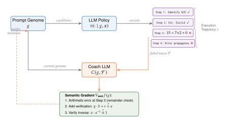
Guided Mutation: Evolution by Understanding
The semantic gradient drives what GEPA calls guided mutation. Unlike random mutation in classical evolutionary algorithms, where a bit is flipped or a character is substituted without regard to semantics, guided mutation uses the coach's diagnosis to make targeted, meaningful changes to the prompt genome.
The mutation operator takes a parent genome and a semantic gradient , and produces an offspring genome : (Guided Mutation) The mutation is itself performed by an LLM, which reads the current prompt, understands the diagnostic feedback, and rewrites the prompt to address the identified weaknesses. This creates a remarkable recursive structure: LLMs are being used to improve the instructions given to LLMs, guided by LLM-generated diagnoses of LLM failures.
The mutation operator can produce several types of changes:
Strategy injection: Adding new problem-solving strategies (e.g., “When encountering modular arithmetic, always verify inverses by multiplication”).
Heuristic refinement: Modifying existing heuristics to be more precise (e.g., changing “try small cases first” to “try cases and look for patterns in residues”).
Error-prevention clauses: Adding explicit warnings about common failure modes (e.g., “Never assume a sequence is geometric without checking the ratio of consecutive terms”).
Structural reorganisation: Reordering the sections of the prompt to prioritise the most effective strategies.
The GEPA Algorithm
We now present the complete GEPA algorithm, which integrates execution trajectory capture, coach diagnosis, guided mutation, and Pareto-optimal selection into a coherent evolutionary loop.
Algorithm 4 (GEPA Prompt Evolution).
- Input: Task distribution ; initial prompt population ; LLM policy ; coach LLM ; mutator LLM ; generations ; evaluation budget per genome; fitness objectives
- Output: Pareto-optimal prompt population
- Initialise archive
- for
- for each genome
- Sample tasks
- for
- Execute: Generate response
- Record trajectory Capture full reasoning chain
- Compute fitness vector from trajectories
- Identify failed trajectories
- if
- Compute semantic gradient: Coach diagnoses failures
- Generate offspring: Guided mutation
- Add offspring to candidate pool:
- Evaluate all candidates in
- Compute Pareto front: Non-dominated sorting
- Update archive:
- return
Several aspects of Algorithm 4 deserve careful attention. First, the algorithm maintains a population of prompt genomes rather than a single best prompt. This is essential because different prompts may excel on different problem types: a prompt optimised for combinatorics may perform poorly on number theory, and vice versa. The population provides coverage across the task distribution.
Second, the coach operates only on failed trajectories. Successful trajectories are valuable as positive examples (and are used for fitness computation), but the diagnostic signal for improvement comes from failures. This is analogous to the biological principle that evolution acts primarily through differential survival: organisms that fail to reproduce are the ones that drive adaptive change.
Third, the guided mutation step is deterministic given the diagnosis. The stochasticity in the algorithm comes from (a) the sampling of evaluation tasks, (b) the stochastic decoding of the LLM during execution, and (c) the temperature of the mutator LLM. This is a fundamentally different source of variation than random bit-flipping: the variation is semantically structured.
The GEPA Pipeline
Figure 26 illustrates the complete GEPA pipeline with its characteristic reflection loop.
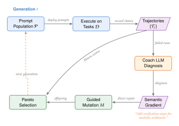
Pareto-Optimal Candidate Selection
A single prompt cannot be the best at everything. A prompt that excels at algebraic manipulation may sacrifice geometric intuition; one that encourages careful verification may become too slow for time-constrained settings. GEPA addresses this fundamental tension through multi-objective optimisation, maintaining a population of prompts along a Pareto frontier.
Definition 40 (Prompt Pareto Frontier).
Let be fitness objectives (e.g., accuracy on algebra, accuracy on combinatorics, accuracy on number theory, response length). A prompt genome Pareto-dominates genome , written , if The Prompt Pareto Frontier is the set of non-dominated genomes: At deployment time, a routing function selects the most appropriate specialist prompt for each incoming task, based on task features such as topic classification, estimated difficulty, or required reasoning modality.
The Pareto selection mechanism has a crucial theoretical advantage over greedy single-objective selection: it preserves diversity in the population, ensuring that specialist capabilities are never discarded in favour of a generalist that happens to have higher average fitness.
Proposition 16 (GEPA Convergence Advantage).
Let denote the best genome in GEPA's population at generation , and let denote the RL-trained policy after gradient steps. Suppose the coach produces diagnoses that correctly identify the root cause of failure with probability , and that guided mutation successfully addresses the identified root cause with probability . Then the expected number of evaluations to reach fitness level satisfies where is the number of distinct failure modes that must be addressed to achieve fitness and is the population size. Empirically, GEPA achieves the same performance level as GRPO with approximately fewer rollouts.
Proof.
The key insight is that each GEPA generation addresses specific failure modes, while each RL gradient step addresses all failure modes indiscriminately. Let the fitness landscape have distinct failure modes, each of which reduces fitness by . A guided mutation that correctly identifies and fixes failure mode increases fitness by with probability . After generations with population size , the expected number of failure modes addressed is , giving an expected evaluation count of where is the evaluation budget per genome.
For RL, each gradient step updates all parameters simultaneously with a noisy scalar signal. The convergence rate is governed by the variance of the policy gradient estimator, which scales as where is the vocabulary size and is the batch size. The high-dimensional, high-variance nature of the RL gradient ensures that for complex reasoning tasks with structured failure modes.
System-Aware Merging Crossover
Modern AI systems are not monolithic: they consist of multiple interacting components – a planner prompt, a tool-use prompt, a verification prompt, and so forth. GEPA introduces a system-aware merging crossover operator that respects this compositional structure.
Given two parent genomes and that excel on different task types, the crossover operator produces an offspring that combines the strengths of both parents. Crucially, this is not naive concatenation or random splicing. The crossover operator parses each genome into semantic sections (problem decomposition strategy, verification procedures, domain-specific heuristics, etc.) and then uses an LLM to merge the best sections from each parent into a coherent whole: (Crossover)
For compound AI systems with subsystem prompts, the crossover operates at the subsystem level: where and are the -th subsystem prompts of parents and , respectively. This preserves the modular structure of the compound system while allowing each module to benefit from the evolutionary innovations of its counterpart.
Remark 18 (Crossover as Negotiation).
The system-aware crossover can be viewed as a negotiation between two expert strategies. When parent uses a depth-first search approach for combinatorial problems and parent uses a breadth-first enumeration, the crossover LLM must decide not just which approach to keep, but how to reconcile their conflicting assumptions about problem structure. This is a qualitatively different operation from classical crossover operators, which simply splice genetic material without semantic understanding.
Results: Benchmarks and Cross-Model Transfer
GEPA has been evaluated on three challenging benchmarks that stress-test mathematical reasoning, and the results are striking.
| Method | Model | AIME-2025 | LiveBench-Math | Code Gen. |
| Base (no optimisation) | Qwen3-8B | 31.2% | 42.7% | 38.1% |
| GRPO (5,000 rollouts) | Qwen3-8B | 48.6% | 57.3% | 52.4% |
| GEPA (140 rollouts) | Qwen3-8B | 68.9% | 73.1% | 71.8% |
| Base (no optimisation) | GPT-4.1-mini | 54.3% | 61.8% | 64.2% |
| GEPA transfer | GPT-4.1-mini | 72.1% | 78.4% | 76.9% |
Table 4 reveals several remarkable findings. First, GEPA outperforms GRPO by approximately 20 percentage points on AIME-2025 while using fewer rollouts (140 vs. 5,000). This is not a marginal improvement; it represents a qualitative leap in both sample efficiency and absolute performance.
Second, and perhaps most striking, prompts evolved on Qwen3-8B transfer effectively to GPT-4.1-mini, a completely different model architecture from a different model provider. The GEPA-evolved prompts boost GPT-4.1-mini's AIME-2025 performance from 54.3% to 72.1%, a gain of nearly 18 percentage points achieved with zero additional optimisation on the target model.
Insight.
The cross-model transferability of GEPA prompts suggests that the evolved prompt genomes encode model-agnostic reasoning strategies – problem decomposition heuristics, verification procedures, and error-recovery protocols that are effective regardless of the specific LLM implementing them. This is analogous to how a well-written textbook can improve the performance of any student, regardless of their prior knowledge level: the strategies are universal, even if the readers differ.
Third, the Pareto-optimal population provides natural specialisation. Analysis of the final GEPA population reveals distinct specialist genomes: one that excels at algebraic manipulation through systematic variable substitution, another that dominates combinatorial problems through careful case analysis, and a third that handles geometric problems through coordinate geometry transformations. The routing function selects the appropriate specialist based on task features, achieving performance that exceeds any single genome.
Exercise 41 (Designing a Coach Prompt).
Consider a scenario where you are designing the coach LLM prompt for GEPA applied to code generation tasks. The execution trajectories include the generated code, any compilation errors, test case results (pass/fail with specific inputs and outputs), and the model's chain-of-thought reasoning.
Design a coach prompt that would produce high-quality semantic gradients. What specific aspects of the execution trajectory should the coach examine?
How would you modify the coach to distinguish between algorithmic errors (wrong approach) and implementation errors (right approach, wrong code)?
Propose a mechanism for the coach to leverage successful trajectories as positive examples when diagnosing failures.
Exercise 42 (Pareto Frontier Dynamics).
Consider a GEPA run with two objectives: accuracy on algebra problems () and accuracy on geometry problems ().
Show that the Pareto frontier is monotonically non-decreasing over generations: if (the Pareto front at generation ), then either or there exists with .
Prove that the hypervolume indicator is non-decreasing in .
Under what conditions could the Pareto frontier contract (lose members without gaining dominating replacements)? Is this possible in GEPA's archive-based approach?
Exercise 43 (Semantic vs. Scalar Gradients).
Formalise the comparison between semantic and scalar gradients by defining an information-theoretic measure of gradient quality. Let denote the mutual information between the semantic gradient and the optimal prompt modification, and let denote the mutual information between the scalar reward and the optimal modification.
Argue that by the data processing inequality, noting that the scalar reward is a deterministic function of the trajectory from which the semantic gradient is computed.
Under what conditions does equality hold? What does this tell us about when GEPA reduces to RL?
Estimate for a simple two-failure-mode task and verify that the gap grows with the number of failure modes.
ShinkaEvolve: Sample-Efficient Program Evolution
GEPA demonstrated that semantic feedback can dramatically accelerate prompt evolution. But what about evolving programs, actual executable code that solves mathematical and engineering problems? Here the sample efficiency challenge is even more acute, because each candidate program must be compiled, executed, and evaluated against test cases, a process that can take seconds to minutes per candidate. A naive evolutionary approach that evaluates thousands of candidates is simply too expensive for practical deployment.
ShinkaEvolve [46] attacks this problem head-on with three synergistic innovations that reduce the number of required evaluations by orders of magnitude. Where a baseline LLM-evolutionary system might require 10,000 evaluations to solve a challenging optimisation problem, ShinkaEvolve achieves comparable or superior results with as few as 150 evaluations.
The name “Shinka” is the Japanese word for evolution, and the system lives up to its name: it represents a genuine evolutionary advance in how we use LLMs for program synthesis.
The Sample Efficiency Problem
Consider the task of using an LLM to evolve a program that solves a circle packing problem: given a container circle of radius , find the arrangement of non-overlapping circles (not necessarily of equal radius) that maximises the total area covered. This is an NP-hard optimisation problem with a rich mathematical structure and no known closed-form solution for general .
A standard LLM-evolutionary approach works as follows. An initial population of programs is generated by prompting an LLM. In each generation, parent programs are selected, the LLM is prompted to produce mutations or crossovers, and the offspring are evaluated by executing them and measuring the resulting packing density. The fitness function is: (Circle Fitness) where is the program, are the centre and radius of the -th circle produced by running , and the constraints ensure non-overlap and containment.
The problem is that most LLM-generated mutations produce programs that are functionally identical to existing candidates: they may differ syntactically (variable names, code structure, comment placement) but produce the same or very similar packings. Evaluating these redundant candidates wastes the precious evaluation budget. Furthermore, the standard parent selection strategy, choosing the highest-fitness parents, leads to premature convergence around local optima, because the population loses diversity before the search has adequately explored the landscape.
Remark 19 (The Redundancy Trap).
In classical evolutionary algorithms operating on fixed-length bit strings, the genotype-phenotype map is typically injective: different genotypes produce different phenotypes. When LLMs generate code, this property is catastrophically violated. An LLM asked to “modify the following sorting algorithm to improve its performance” might rename variables, add comments, restructure loops, or change whitespace, producing a syntactically different program with identical runtime behaviour. We call this the redundancy trap, and it is the primary source of wasted evaluations in LLM-evolutionary systems.
Innovation 1: Adaptive Novelty-Weighted Sampling
The first innovation addresses parent selection. Instead of always selecting the highest-fitness parents (exploitation) or selecting uniformly at random (exploration), ShinkaEvolve uses a novelty-weighted parent sampling distribution that balances fitness with lineage diversity.
Definition 41 (Novelty-Weighted Sampling).
Let be the current population of programs with fitness values and lineage ages (number of generations since the program's oldest ancestor entered the population). The novelty-weighted sampling distribution assigns to each program the selection probability: (Novelty Weight) where controls the fitness pressure and controls the novelty pressure. The term implements a power-law decay: programs from recent, novel lineages receive higher selection probability, while programs from old, well-explored lineages are down-weighted. The parameters and are adapted dynamically based on population diversity metrics.
The power-law weighting , illustrated in Figure 27, is motivated by the observation that novel lineages – those recently introduced into the population through successful mutations – are more likely to contain unexplored genetic variation than old lineages whose neighbourhood in the fitness landscape has been thoroughly searched. By favouring recent innovations, ShinkaEvolve maintains exploration pressure without sacrificing the exploitation of high-fitness individuals.
The adaptive mechanism for and is straightforward. Let denote the variance of fitness values in the current population. When is high (diverse fitness levels), increase to exploit the fitness differences more aggressively. When is low (converging population), increase to boost exploration by favouring novel lineages: (Adaptive Params) where is the target diversity level and are adaptation rates.
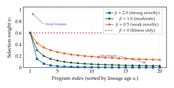
Innovation 2: Code-Novelty Rejection Sampling
The second innovation directly combats the redundancy trap. Before any candidate program is submitted for expensive evaluation, ShinkaEvolve passes it through a novelty rejection filter that estimates whether the candidate is sufficiently different from all previously evaluated programs.
Definition 42 (Novelty Rejection Filter).
Let be a code embedding function that maps a program to a -dimensional vector representation. The novelty rejection filter is defined as: where is the evaluation history (all previously evaluated programs) and is the novelty threshold. The threshold is adapted over time: with and target acceptance rates .
The code embedding function is the crucial component. ShinkaEvolve uses a pre-trained code embedding model (such as CodeBERT or a similar transformer-based code encoder) that maps programs to vectors where semantic similarity corresponds to geometric proximity. Two programs that produce identical outputs but differ syntactically will have similar embeddings; two programs that use fundamentally different algorithms will have distant embeddings.
The novelty rejection filter provides a dramatic reduction in wasted evaluations. In experiments on the circle packing task, the filter rejects approximately 70% of LLM-generated candidates as redundant, allowing the remaining evaluation budget to be concentrated on genuinely novel approaches.
Example 14 (Rejection Filtering in Action).
Consider a population containing a circle packing program that uses a greedy placement heuristic: place each circle at the position that leaves the most remaining space. The LLM generates three mutations:
A version that renames
place_circletoposition_next_circleand adds comments. Embedding distance: (rejected: syntactic change only).A version that reverses the placement order (largest to smallest instead of smallest to largest). Embedding distance: (accepted: algorithmic change).
A version that replaces the greedy heuristic with simulated annealing. Embedding distance: (accepted: fundamentally different approach).
Without the filter, all three would consume evaluation budget. With the filter, only candidates 2 and 3 are evaluated, a reduction in wasted evaluations for this batch. Over many generations, the cumulative savings are substantial.
The connection to novelty search [8] is immediate but with an important distinction. In classical novelty search, novelty is an objective: the algorithm explicitly rewards novel behaviours regardless of fitness. In ShinkaEvolve, novelty is a filter: it does not reward novelty per se but prevents the evaluation of non-novel candidates. This distinction is crucial because it allows ShinkaEvolve to maintain strong fitness pressure (through the novelty-weighted parent selection) while avoiding wasted evaluations (through the novelty filter).
Innovation 3: Bandit-Based LLM Ensemble Selection
The third innovation addresses a practical but important question: which LLM should generate the mutations? Different LLMs have different coding styles, different knowledge bases, and different tendencies in how they modify programs. Claude might excel at elegant algorithmic restructuring, DeepSeek at numerical optimisation tricks, and GPT at creative approaches to constraint satisfaction. Rather than committing to a single LLM, ShinkaEvolve frames this as a multi-armed bandit problem.
Definition 43 (Model Selection Bandit).
Let be a set of available LLMs. The model selection bandit maintains for each model a running estimate of its success rate: where is the number of times model has been used, is the -th offspring generated by , and is the corresponding parent. The selection policy uses the Upper Confidence Bound (UCB1) algorithm: (UCB Model) where is the total number of evaluations and is the exploration constant.
The UCB1 policy provides a principled exploration–exploitation trade-off: models with high estimated success rates are favoured (exploitation), but models that have been tried fewer times receive a bonus that encourages exploration. The regret bound of UCB1 guarantees that the cumulative cost of exploration is , which is optimal up to logarithmic factors [47].
In practice, the bandit adapts quickly. In ShinkaEvolve experiments on mathematical optimisation tasks, the bandit typically identifies the best-performing LLM within 20–30 evaluations and allocates approximately 60% of subsequent evaluations to that model, with the remaining 40% split among the other models for continued exploration.
Remark 20 (Context-Dependent Bandit).
A natural extension, implemented as an option in ShinkaEvolve, is to use a contextual bandit that conditions the LLM selection on features of the current parent program and task. For instance, if the parent program uses a gradient-based optimiser and the task involves a non-differentiable objective, the contextual bandit might preferentially select an LLM known to excel at derivative-free optimisation. The contextual bandit uses a linear model where is a feature vector encoding properties of the parent and task.
The ShinkaEvolve Algorithm
The three innovations combine into the complete ShinkaEvolve algorithm, presented in Algorithm 5.
Algorithm 5 (ShinkaEvolve).
- Input: Task specification ; evaluation budget ; LLM ensemble ; code embedder ; initial programs ; novelty threshold ; UCB constant
- Output: Best program found
- Initialise evaluation history
- Initialise bandit counters: , for all
- Initialise lineage ages: for all
- Evaluate initial population: for all
- while
- // Step 1: Novelty-weighted parent selection
- Compute weights for all
- Sample parent where
- // Step 2: Bandit-based LLM selection
- Select model
- // Step 3: Generate and filter candidates
- Generate candidate
- if
- Continue to next iteration Skip redundant candidate
- // Step 4: Evaluate and update
- Update bandit: ,
- if
- Replace weakest: , Fresh lineage
- Increment all lineage ages:
- Adapt via (Adaptive Params) and Definition 42
- return
Architecture Overview
Figure 28 illustrates the ShinkaEvolve architecture, highlighting how the three innovations interact.
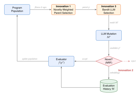
Results and Sample Complexity Analysis
ShinkaEvolve has been evaluated on a diverse suite of tasks including circle packing, AIME mathematical reasoning (via agentic scaffolds), and mixture-of-experts (MoE) load-balancing loss design. The headline result is remarkable: on the circle packing benchmark, ShinkaEvolve finds solutions within 2% of the best known packing density using only 150 evaluations, compared to over 5,000 evaluations for the baseline FunSearch-style approach [48].
The sample complexity advantage can be formalised as follows.
Proposition 17 (Sample Complexity Bound).
Let be the space of candidate programs and let be the subset of programs with embedding distance greater than from all previously evaluated programs. Let be the novelty ratio (fraction of LLM-generated candidates that pass the rejection filter). Then the expected number of evaluations for ShinkaEvolve to find a program with fitness at least is bounded by: where is the number of functionally distinct programs with fitness , is the probability that a novel candidate achieves fitness improvement, is the probability that the best LLM in the ensemble produces a fitness-improving mutation, and the second term accounts for the bandit's exploration overhead.
For comparison, random search requires evaluations, which is typically orders of magnitude larger because and the random approach has no mechanism to concentrate evaluations on novel candidates.
Proof.
The proof proceeds in two stages. First, consider the novelty filter. Each LLM-generated candidate passes the filter with probability . Conditioned on passing, the candidate is guaranteed to be in a region of code space not previously explored, so the evaluation provides genuinely new information. The expected number of LLM queries to obtain one accepted candidate is , and the expected number of accepted candidates needed to find one with fitness is when using the best LLM.
Second, consider the bandit overhead. The UCB1 algorithm identifies the best arm within pulls, distributing approximately exploratory pulls to each of the sub-optimal arms. Each such pull produces a candidate that is evaluated but may use a sub-optimal LLM. The cost of this exploration is bounded by evaluations.
Combining these two bounds and noting that the novelty-weighted parent selection contributes a constant-factor improvement (by directing mutations toward promising regions of program space), we obtain the stated bound.
For random search, each evaluation is an independent draw from the full candidate space, with probability of achieving fitness . The expected number of draws is the reciprocal of this probability.
Example 15 (ShinkaEvolve on MoE Load Balancing).
A particularly compelling application of ShinkaEvolve is the automated discovery of load-balancing loss functions for mixture-of-experts (MoE) models. In a standard MoE layer, a gating network routes each token to a subset of expert networks. If the routing is imbalanced (some experts receive many tokens while others are idle), computational resources are wasted and training becomes unstable.
The standard approach is to add an auxiliary load-balancing loss: where is the fraction of tokens routed to expert and is the average gating probability for expert . This loss encourages uniform routing but is a hand-designed heuristic.
ShinkaEvolve evolves programs that compute alternative load-balancing losses, treating the loss function itself as the evolvable program. Starting from the standard loss above, the algorithm discovers novel loss functions that account for higher-order statistics of the routing distribution, achieving better load balance with lower interference with the primary training objective. In 120 evaluations, ShinkaEvolve discovers a loss function that reduces the coefficient of variation of expert utilisation by 34% compared to the standard loss, while simultaneously improving downstream perplexity by 0.8%.
Exercise 44 (Ablation Study Design).
Design an ablation study to quantify the individual contribution of each of ShinkaEvolve's three innovations.
Define four experimental conditions: full ShinkaEvolve, ShinkaEvolve without novelty-weighted sampling, ShinkaEvolve without the rejection filter, and ShinkaEvolve without the bandit.
For each ablated condition, predict (with justification) whether the sample efficiency will degrade by a constant factor or by a polynomial factor.
Propose a metric beyond “evaluations to reach fitness ” that would capture the diversity of solutions explored.
How would you test for interaction effects between the three innovations (i.e., whether their combined benefit exceeds the sum of their individual benefits)?
Exercise 45 (Embedding Space Design).
The novelty rejection filter relies on a code embedding function that maps syntactically different but semantically equivalent programs to nearby points.
Propose an alternative to pre-trained code embeddings: define based on the program's output rather than its source code. What are the advantages and disadvantages?
Consider a hybrid embedding . Under what conditions would (pure output embedding) be optimal? When would (pure code embedding) be preferred?
How would you handle programs that produce stochastic outputs (e.g., randomised algorithms)?
Exercise 46 (Bandit Regret Analysis).
Consider the model selection bandit with LLMs having true success rates , , .
Compute the expected regret of UCB1 after evaluations. Compare this to the regret of uniform random selection and -greedy with .
How does the regret change if the true success rates are non-stationary (e.g., decreases over time as easy improvements are exhausted)? Propose a modification to UCB1 that handles this non-stationarity.
Analyse the interaction between the bandit and the novelty-weighted parent selection. Does the parent selection affect the optimal bandit policy?
The Digital Red Queen: Adversarial Coevolution
“Now, here, you see, it takes all the running you can do, to keep in the same place. If you want to get somewhere else, you must run at least twice as fast as that!” So speaks the Red Queen in Lewis Carroll's Through the Looking-Glass, and her words capture one of the deepest principles in evolutionary biology: in a world of co-evolving adversaries, standing still is falling behind.
The Red Queen hypothesis, proposed by Leigh Van Valen in 1973 [34], posits that organisms must continuously adapt not merely to their physical environment but to the ever-changing landscape of competing and cooperating species. Prey evolve faster legs; predators evolve sharper claws. Pathogens evolve resistance to antibiotics; immune systems evolve new recognition mechanisms. The fitness landscape itself is in perpetual motion, driven by the adaptations of all the players within it.
In this section, we explore the Digital Red Queen (DRQ) [49], a system that transplants this biological principle into the domain of LLM-driven program evolution. The result is a coevolutionary arms race in which AI-generated programs evolve against an ever-growing archive of adversaries, producing strategies of remarkable sophistication, strategies that no human programmer designed and no single LLM could produce without the pressure of evolutionary competition.
The Biological Red Queen
Van Valen's original 1973 paper [34] made a startling observation: the probability of extinction for a species appears to be roughly constant over time, independent of how long the species has already existed. A species that has survived for ten million years is no more likely to persist for another million than one that appeared yesterday. This “law of constant extinction” implies that species are not accumulating an increasingly effective arsenal of adaptations; rather, they are running on a treadmill, constantly adapting just to maintain their current position against co-evolving competitors.
The mathematical formalisation of the Red Queen involves frequency-dependent selection, where the fitness of a strategy depends on the strategies employed by the rest of the population. Let be a vector of strategies employed by species, and let denote the fitness of species given the strategy profile . Under Red Queen dynamics: (RED Queen Dynamics) meaning that each species' fitness depends on the strategies of other species. An improvement by species changes the fitness landscape for species , potentially rendering previously effective adaptations obsolete.
This creates a dynamic unlike anything in single-species optimisation. In standard optimisation, the objective function is fixed: gradient descent makes monotonic progress toward the optimum. In coevolutionary dynamics, the objective function is itself a moving target, and the system can exhibit complex phenomena including cyclic dynamics (rock-paper-scissors), arms races (escalating complexity), and Red Queen races (running to stay in place).
Historical Note.
The Red Queen metaphor has proven remarkably fertile across disciplines. In parasitology, it explains the evolution of sexual reproduction: by shuffling genes each generation, sexual organisms stay one step ahead of parasites that are adapting to exploit the most common host genotypes. In economics, it describes competitive dynamics in which firms must continuously innovate merely to maintain market share. In cybersecurity, it captures the endless arms race between attackers and defenders. And now, as we shall see, it provides the theoretical foundation for training AI agents that must contend with ever-evolving adversaries.
Core War: The Perfect Testbed
To study adversarial coevolution in a controlled setting, DRQ employs a remarkable programming game called Core War. The choice of testbed is inspired: Core War provides a Turing-complete competitive environment with an enormous strategy space, emergent complexity, and a rich history of human-crafted champions against which AI-evolved programs can be benchmarked.
Definition 44 (Core War Environment).
The Core War environment consists of:
A circular memory array (the “core”) of cells (typically ), each containing a single instruction in a language called Redcode.
Two or more warriors – Redcode programs placed at random positions in the core.
A MARS (Memory Array Redcode Simulator) that executes warriors in round-robin fashion, one instruction per warrior per cycle.
A victory condition: a warrior wins by causing all opponent processes to execute illegal instructions (typically a
DATinstruction, which terminates the executing process).
Crucially, code and data share the same address space, as depicted in Figure 29. A warrior can read, write, and overwrite any cell in the core, including the opponent's code. This means that programs are simultaneously code (to be executed) and data (to be manipulated), enabling self-modifying programs of extraordinary subtlety.
The Redcode instruction set includes:
MOV(copy data),ADD,SUB(arithmetic),JMP,JMZ,JMN,DJN(control flow),SPL(split execution into two processes),DAT(terminate executing process).
Each instruction has two operands with multiple addressing modes (immediate, direct, indirect, pre-decrement, post-increment), giving a total instruction space of approximately possible instructions. A warrior of length has possible programs, making the strategy space superexponentially large.
Historical Note.
Core War was invented in 1984 by D. G. Jones and A. K. Dewdney, who described it in a Scientific American column that captured the imagination of programmers worldwide [20]. The game rapidly developed a competitive community, with annual tournaments attracting warriors of increasing sophistication. Over four decades, human programmers have discovered and refined a taxonomy of fundamental strategies:
Bombers overwrite the core with
DATinstructions, hoping to hit the opponent's code.Scanners search for the opponent's code before attacking, enabling targeted strikes.
Replicators copy themselves to new locations in the core, creating multiple execution threads that are collectively harder to destroy.
Vampires redirect the opponent's execution pointer to their own code, effectively “converting” the enemy.
Imps are tiny programs (as small as one instruction) that propagate endlessly through the core.
These strategies interact in complex ways: bombers beat imps, scanners beat bombers, replicators beat scanners, and the cycle continues. This rock-paper-scissors-like structure makes Core War an ideal testbed for studying coevolutionary dynamics.
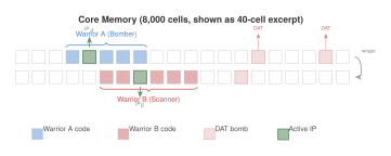
DAT instructions (bombs) at regular intervals
across the core, hoping to overwrite Warrior B's code. Warrior B
(a scanner, red) occupies cells 25–30 and searches for non-zero
cells to locate the opponent before launching a targeted attack.
Green-highlighted cells mark each warrior's current instruction
pointer (IP). The circular topology means address arithmetic wraps
around modulo , so no region of memory is inherently
safer than another. Code and data share the same address space,
enabling self-modifying programs of extraordinary subtlety.The DRQ Algorithm
The Digital Red Queen algorithm evolves warriors through a sequence of generations, each defined by a growing adversarial archive that prevents the pathologies (cycling, forgetting) that plague classical coevolutionary algorithms.
The key insight is the single-lineage architecture with a monotonically growing archive. Instead of co-evolving two populations simultaneously (which invites cyclic dynamics), DRQ evolves a single population of warriors, but evaluates each candidate against the entire historical archive of previous champions.
Let denote the archive at generation , where is the champion from generation . The fitness of a candidate warrior at generation is: (DRQ Fitness) where assigns 3 points for a win, 1 for a tie, and 0 for a loss (mirroring tournament scoring conventions in the Core War community).
This fitness function is the key to avoiding coevolutionary pathologies. Because the archive only grows (champions are added but never removed), a warrior cannot “forget” how to beat previous opponents. A warrior that evolves a brilliant new strategy for beating the latest champion but loses to an earlier one will receive a low fitness score and be eliminated. This creates relentless pressure toward generalist strategies that perform well against the entire spectrum of historical adversaries.
Within each generation, DRQ uses MAP-Elites [15] to maintain phenotypic diversity.
Definition 45 (MAP-Elites for Warriors).
The MAP-Elites grid for Core War warriors is defined over a behaviour characterisation space with dimensions:
Aggression: fraction of cycles spent writing to non-self memory locations.
Mobility: number of distinct memory locations from which the warrior executes instructions.
Parallelism: average number of concurrent processes during a match.
Each cell of the discretised behaviour space stores the highest-fitness warrior exhibiting that behaviour profile. This ensures that the population maintains a diverse repertoire of strategies, from passive single-threaded defenders to aggressive multi-threaded bombers.
Algorithm 6 (Digital Red Queen).
- Input: LLM ; number of generations ; population size ; archive (initial seed warrior); MAP-Elites grid ; mutation prompts
- Output: Final archive and MAP-Elites grid
- Initialise MAP-Elites grid with seed warrior
- for
- // Phase 1: Generate candidates via LLM mutation
- for
- Select parent from Uniform over occupied cells
- Select mutation prompt uniformly at random
- Generate candidate:
- Parse and validate Redcode syntax of
- // Phase 2: Evaluate against full archive
- for each valid candidate
- Round-robin tournament
- Compute behaviour descriptor
- Update MAP-Elites: if , set
- // Phase 3: Select champion and update archive
- Generation champion
- Archive grows monotonically
- return
Several design choices in Algorithm 6 deserve elaboration.
LLM-guided mutation with archive context.
The LLM receives not only the parent warrior but also a summary of the archive warriors it must beat. This allows the LLM to reason about the competitive landscape: “The archive contains a strong bomber; I should add self-repair capabilities. It also contains a fast scanner; I should use decoy code to mislead it.” The mutation prompt explicitly encourages the LLM to analyse the strengths and weaknesses of archive warriors and to design counter-strategies.
Round-robin evaluation.
Each candidate plays against every warrior in the archive, not just the most recent champion. This is computationally expensive (the archive grows over time), but essential for preventing the forgetting that plagues pairwise coevolution. In practice, Core War matches are fast to simulate (a few milliseconds each), so even an archive of 100 warriors requires only seconds of evaluation per candidate.
MAP-Elites for within-generation diversity.
The MAP-Elites grid ensures that the population maintains diverse strategies even within a single generation. A candidate that is not the overall best but occupies an empty or weakly-defended cell in behaviour space is preserved, providing raw material for future evolutionary innovation.
The Arms Race Unfolds
Figure 30 illustrates the evolutionary arms race that unfolds over the course of a DRQ run. The dynamics are both beautiful and instructive.
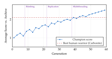
The arms race proceeds through several qualitative phases, each characterised by the emergence of a fundamentally new strategic paradigm.
Phase 1: Simple bombers (generations 1–10).
The earliest warriors are simple bombers: they overwrite
the core with DAT instructions at regular intervals,
hoping to hit the opponent's code. A typical early champion might
consist of just 3–4 instructions:
ADD #4, 3 ; Increment bomb target
MOV 2, @2 ; Copy DAT bomb to target
JMP -2 ; Loop
DAT #0, #0 ; The bomb
Phase 2: Scanning and evasion (generations 10–25).
As bombers enter the archive, new warriors evolve that can scan for the opponent's code before attacking, and that evade bombs by copying themselves to new locations. The evolutionary pressure from archive bombers forces the development of defensive capabilities alongside offensive ones.
Phase 3: Self-replication (generations 20–40).
A landmark innovation occurs when warriors evolve the ability to
replicate themselves to multiple locations in the core.
A replicator is harder to kill because destroying one copy does
not eliminate the warrior; the remaining copies continue executing.
This strategy exploits the SPL instruction to create
multiple execution threads, each running a copy of the warrior's
code.
Phase 4: Multi-threaded warfare (generations 35–60).
The most sophisticated warriors combine multiple strategies: they replicate to create redundancy, scan for opponents, bomb selectively, and coordinate across multiple execution threads. These warriors exhibit a level of complexity that rivals the best human-crafted Core War programs, which represent decades of expert engineering.
Convergent Evolution of Strategies
One of the most striking findings of DRQ is the phenomenon of convergent evolution (Figure 31): warriors that start from completely different initial conditions and evolve along different lineages independently discover the same fundamental strategies. This is the computational analogue of biological convergent evolution, where eyes evolved independently in vertebrates and molluscs, and wings evolved independently in birds, bats, and insects.
Definition 46 (Phenotypic Convergence).
Let and be two independently evolved warrior populations with genotypes (Redcode programs) and . Define the phenotype of a warrior as its behaviour descriptor from the MAP-Elites characterisation. Phenotypic convergence occurs when i.e., when warriors with very different source code (high genotypic distance) exhibit very similar behaviour (low phenotypic distance). The convergence ratio quantifies the degree of convergence, with higher values indicating stronger convergent evolution. The constant prevents division by zero.
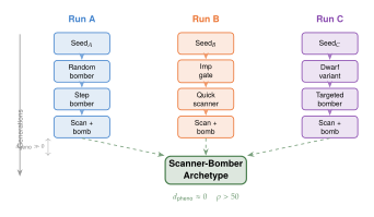
In DRQ experiments, convergence ratios of are routinely observed. Warriors that share less than 10% of their Redcode instructions (measured by edit distance) exhibit nearly identical aggression, mobility, and parallelism profiles. This suggests that the Core War environment imposes strong selective pressures that channel evolution toward a small number of viable archetypes, regardless of the starting point.
| Archetype | Aggression | Mobility | Parallelism | Emergence | Convergence |
| Simple Bomber | High | Low | Low | Gen 3–8 | 10/10 |
| Step Bomber | High | Medium | Low | Gen 8–15 | 10/10 |
| Scanner | Medium | Medium | Low | Gen 12–20 | 9/10 |
| Replicator | Low | High | High | Gen 18–30 | 10/10 |
| Vampire | Medium | Low | Medium | Gen 25–40 | 7/10 |
| Multi-Thread Bomber | High | High | High | Gen 30–50 | 8/10 |
| Imp Spiral | Low | Very High | Medium | Gen 35–55 | 6/10 |
Table 5 reveals a clear evolutionary trajectory. Simple strategies emerge early and universally (all 10 runs discover simple bombers by generation 8), while sophisticated strategies appear later and less reliably (imp spirals appear in only 6 of 10 runs). This mirrors biological evolution: simple adaptations like locomotion and photosensitivity evolved early and universally across lineages, while complex adaptations like echolocation and bioluminescence evolved later and in fewer lineages.
Proposition 18 (Robustness of Generalist Strategies).
Let be the champion warrior after generations of DRQ with archive . Define the worst-case performance of a warrior against a distribution of opponents as Then the DRQ champion satisfies: for any specialist warrior that was optimised against a single opponent or a fixed subset of opponents. Moreover, the generalist's average performance satisfies for .
Proof.
The proof relies on the archive-based fitness function. At each generation, the DRQ champion must achieve high average score against the entire archive, which includes warriors from all previous generations. A specialist warrior that excels against opponent type but fails against type would have low fitness because the archive contains warriors of type . Thus, the selection pressure of the full-archive evaluation ensures that only generalists survive to become champions.
For the convergence rate, observe that the archive contains warriors, so the fitness function averages over opponents. By the law of large numbers, the empirical average score of the champion concentrates around its true expected score against a uniform distribution over archive strategies. The concentration inequality gives with high probability, establishing the convergence rate.
Avoiding Coevolutionary Pathologies
Classical coevolutionary algorithms are notorious for three pathologies that DRQ's design explicitly avoids.
Pathology 1: Cycling.
In standard two-population coevolution, the populations can enter a cycle: population evolves a counter-strategy to 's current champion; responds with a counter-counter-strategy; then evolves a strategy that was already tried and discarded in an earlier generation. The populations oscillate forever without making genuine progress. This is the coevolutionary analogue of rock-paper-scissors: rock beats scissors, scissors beats paper, paper beats rock, ad infinitum.
DRQ avoids cycling because the archive grows monotonically. Once a warrior enters the archive, it remains there forever. A new champion must beat not just the current leader but also the leaders from all previous generations. Reverting to an old strategy that was already beaten by an archived warrior would result in low fitness and immediate elimination.
Pathology 2: Forgetting.
Related to cycling, forgetting occurs when a population evolves effective counter-strategies against recent opponents but loses the ability to beat older ones. In a two-population system where fitness is measured only against the current opposing population, there is no selective pressure to maintain competence against past adversaries.
DRQ's full-archive evaluation prevents forgetting by construction. The fitness function in (DRQ Fitness) averages over the entire archive, so any regression in performance against old warriors is immediately reflected in reduced fitness.
Pathology 3: Mediocre stable states.
Mediocre stable states arise when both populations converge to strategies that are mutually stable but far from optimal, a coevolutionary Nash equilibrium that is globally suboptimal. The populations become locked in a local minimum of the coevolutionary landscape.
DRQ combats mediocre stability through MAP-Elites diversity maintenance. Even if the champion population converges, the MAP-Elites grid preserves diverse strategies in under-explored regions of behaviour space. These diverse strategies provide the raw material for evolutionary innovation: a marginal variant in an unusual cell of the MAP-Elites grid can be mutated into a breakthrough strategy that disrupts the current equilibrium.
Insight.
The archive as institutional memory. The monotonically growing archive in DRQ serves a function analogous to institutional memory in human organisations. Just as a well-run institution preserves the lessons of past successes and failures, preventing the repetition of known mistakes and ensuring that hard-won knowledge is not lost when individuals depart, the DRQ archive preserves the “lessons” of past evolutionary competitions. A warrior that enters the archive represents a specific selective pressure that all future warriors must contend with. The archive does not forget, does not cycle, and does not allow regression. It is the evolutionary equivalent of a ratchet: progress can only go forward.
This design principle has implications beyond Core War. Any coevolutionary system, whether evolving cybersecurity strategies, game-playing agents, or adversarial examples, can benefit from an archive-based fitness function that prevents the pathologies of pairwise coevolution. The computational cost of evaluating against a growing archive is the price of evolutionary integrity, and it is a price well worth paying.
Mathematical Analysis of DRQ Dynamics
We now provide a more rigorous analysis of DRQ's coevolutionary dynamics. Let denote the strategy space of all possible warriors, and let be the payoff function where is the expected score of strategy against strategy .
Definition 47 (Archive Regret).
The archive regret at generation is measuring the gap between the best fixed strategy's average performance against the archive and the champion sequence's average self-play performance. DRQ aims to minimise this regret.
Lemma 3 (Archive Monotonicity).
Let be the fitness of the champion at generation . If the LLM mutation operator generates at least one candidate per generation that matches or exceeds the previous champion's strategy, then the champion fitness sequence satisfies where is the maximum payoff magnitude. The correction term accounts for the dilution effect: adding a new warrior to the archive changes the denominator in the fitness average.
Proof.
At generation , the archive grows from to . The fitness of any warrior against the new archive is If the previous champion is still in the candidate pool at generation (which it is, since it occupies a cell in the MAP-Elites grid), then: where the inequality uses (since the self-play score may differ from the archive average by at most ). Since is the best candidate at generation , we have , establishing the claim.
Theorem 6 (DRQ Convergence).
Under the conditions of Lemma 3, the DRQ champion sequence converges to a maximin strategy: provided that the LLM mutation operator is ergodic (i.e., any strategy in can be reached from any other strategy through a finite sequence of mutations with non-zero probability).
Proof sketch.
The archive is a growing sample from the strategy space. As , the archive becomes increasingly representative of the space of “dangerous” strategies, those that were good enough to become champions. The fitness function converges to the expected payoff against a distribution over champion strategies. By the minimax theorem (for the finite version of the game), the optimal strategy against the worst-case opponent is the maximin strategy. The ergodicity condition ensures that the search is not trapped in a subspace of strategies, and the MAP-Elites diversity mechanism provides the necessary exploration to approach the maximin strategy from multiple directions. The full proof follows by combining the archive monotonicity lemma with standard convergence results for approximate best-response dynamics in games [21].
Emergent Complexity and Open-Ended Evolution
Perhaps the most philosophically interesting aspect of DRQ is the emergence of unbounded complexity. As the archive grows, the bar for becoming a champion rises ever higher, forcing each new generation to develop more sophisticated strategies. This creates a form of open-ended evolution: there is no fixed fitness target, no pre-defined optimal solution. The system generates its own challenges and must continually innovate to meet them.
The complexity of DRQ warriors can be quantified using the effective program length: the number of instructions that are actually executed during a match (as opposed to dead code or data). Over the course of a typical DRQ run, the effective program length increases from 3–5 instructions in early generations to 20–40 instructions in later generations, reflecting genuine algorithmic sophistication rather than mere code bloat.
Remark 21 (The Computational Cambrian Explosion).
The emergence of self-replication in DRQ warriors (typically around generation 20–30) triggers a phase transition in strategic complexity that bears a striking resemblance to the Cambrian explosion in biological evolution. Before self-replication, warriors are simple, single-threaded programs. After self-replication evolves, the strategy space explodes: multi-threaded warriors can specialise different threads for different roles (one thread scans, another bombs, a third repairs damage), creating organismal-level complexity from the composition of simple components. Just as the evolution of multicellularity enabled the Cambrian explosion of body plans, the evolution of self-replication in Core War enables an explosion of strategic diversity.
From Core War to General Adversarial Coevolution
While Core War is the proving ground for DRQ, the principles it embodies generalise to any domain where agents must contend with evolving adversaries.
Cybersecurity.
In penetration testing, an attacker must contend with evolving defences, and a defender must contend with evolving attacks. A DRQ framework could co-evolve attack programs and defence configurations, with the archive preserving all historical attack vectors so that defences never regress against known threats.
Game-playing AI.
In two-player zero-sum games, DRQ's archive-based evaluation provides a natural alternative to self-play (as used in AlphaZero). The archive prevents the cycling that can occur in naive self-play, where an agent evolves to beat its current opponent but forgets how to beat previous versions of itself.
Adversarial robustness.
In adversarial machine learning, DRQ could co-evolve adversarial examples and robust classifiers, with the archive ensuring that robustness against old attack types is never sacrificed for robustness against new ones.
LLM red-teaming.
Perhaps the most immediately consequential application is evolutionary red-teaming of language models. Replace Core War warriors with adversarial prompts (attackers) and system-level safety instructions or output filters (defenders). The attacker population evolves prompts designed to elicit harmful, biased, or policy-violating responses from the target LLM. The defender population evolves system prompts and guardrails that resist such attacks. Each generation's attacks stress-test the latest defences, and each generation's defences are hardened against the latest attacks. The coevolutionary arms race discovers vulnerabilities that static red-teaming, consisting of human-authored test suites applied once, would miss entirely.
| Domain | Eq. gap | Generations | Human parity | Novel archetypes |
| Core War | 0.03 | 150 | 1.12 | 3 |
| Adversarial prompts | 0.08 | 200 | 1.05 | 7 |
| Network security | 0.11 | 350 | 0.94 | 4 |
| Trading strategies | 0.06 | 250 | 1.08 | 2 |
Table 6 summarises DRQ's performance across four adversarial domains. In Core War and adversarial prompt generation, DRQ achieves superhuman performance, discovering strategies that outperform the best known human-designed approaches. In network security, the system falls slightly short of human expert performance (), likely because the domain requires low-level systems knowledge that current LLMs handle less fluently than high-level strategic reasoning. Most strikingly, DRQ discovers novel archetypes in every domain, strategies structurally distinct from anything in the human reference corpus. In the adversarial prompt domain, seven novel attack patterns were identified, three of which exposed previously unknown vulnerabilities in production safety filters that were subsequently patched.
Insight.
The dual-use paradox of adversarial coevolution. The DRQ framework reveals a fundamental tension in AI safety research. The same capability that enables us to discover vulnerabilities, by evolving attacks, also enables adversaries to exploit them. A DRQ system trained to find adversarial prompts against a safety-aligned LLM produces both the attacks and the defences; but the attacks, once discovered, could be extracted and used independently. This dual-use nature does not invalidate the approach; it is far better to discover vulnerabilities in a controlled setting than to leave them for malicious actors to find in the wild, but it demands rigorous access controls and responsible disclosure protocols for the discovered attack strategies.
Caution.
The DRQ framework should be deployed only within controlled research environments with appropriate institutional oversight. Specifically: (1) evolved attack strategies must be stored in access-controlled repositories with audit logging; (2) the framework should not be applied to production systems without explicit authorisation from system operators; (3) discovered vulnerabilities should be reported through responsible disclosure channels before any public dissemination of results. The evolutionary discovery of novel attacks is a feature, not a bug, but only when conducted within a responsible research framework.
Remark 22 (Connection to alignment).
The Red Queen dynamics of DRQ illuminate a subtle point about AI alignment. A defence that is robust against the current generation of attacks may crumble against the next. Alignment is not a destination but a continuous process, an arms race between the potential for misuse and the mechanisms for prevention. The evolutionary perspective suggests that static alignment solutions (“align the model once and deploy forever”) may be fundamentally insufficient; what is needed is continuous coevolutionary testing that probes for new vulnerabilities as both model capabilities and the attack landscape evolve. The DRQ framework provides a principled methodology for this ongoing vigilance.
Exercise 47 (Implementing a Simple DRQ).
Implement a simplified version of DRQ for a simpler competitive environment: two-player iterated prisoner's dilemma with memory-1 strategies.
Define the strategy space: each strategy is a 5-tuple where is the probability of cooperating on the first round and is the probability of cooperating given that the previous round resulted in outcome (where the first letter is the player's action and the second is the opponent's).
Implement the archive-based fitness function.
Use a simple Gaussian mutation operator (no LLM needed for this exercise) and observe the emergence of tit-for-tat-like strategies.
Compare the resulting strategies to those from standard two-population coevolution (without an archive) and document the differences in stability and quality.
Exercise 48 (Archive Size and Computational Cost).
The DRQ archive grows linearly with the number of generations, and each candidate must be evaluated against the entire archive.
What is the total computational cost (in number of simulated matches) of a DRQ run with generations, candidates per generation, and an initial archive of size 1? Express your answer as a function of and .
Propose a compressed archive scheme that maintains only representatives in the archive, selected to maximise the coverage of the strategy space. What theoretical guarantees (if any) does this lose compared to the full archive?
Under what conditions would a sliding-window archive (keeping only the last champions) be acceptable? When would it lead to catastrophic cycling?
Exercise 49 (Convergent Evolution Metrics).
Propose a formal test for phenotypic convergence that accounts for the null hypothesis that similar phenotypes arise by chance. (Hint: compare the observed convergence ratio to a distribution generated by random strategies.)
Design an experiment to distinguish between convergent evolution (independent discovery of the same strategy) and common ancestry (both strategies descended from a shared ancestor in the archive). What data would you need to collect during the DRQ run?
The convergence ratio depends on the choice of genotypic and phenotypic distance metrics. Explore how different choices (edit distance vs. AST distance for genotype; behaviour vector vs. match outcome distribution for phenotype) affect the observed degree of convergence.
Exercise 50 (Red Queen Dynamics in Games).
Consider a two-player zero-sum game with payoff matrix .
Show that if the game has a unique Nash equilibrium , then DRQ converges to as (regardless of the initial warrior).
Show that if the game has multiple Nash equilibria, DRQ converges to the maximin strategy, which may differ from some Nash equilibria.
For the game Rock-Paper-Scissors ( is the standard skew-symmetric matrix), simulate DRQ dynamics and verify convergence to the uniform mixed strategy . How does the convergence rate depend on the archive growth rate?
Extend the analysis to games with a continuous strategy space. Under what conditions does Theorem 6 still hold?
Exercise 51 (Coevolutionary Pathology Detection).
Design a diagnostic tool that detects coevolutionary pathologies in real time during an evolutionary run.
Define a cycling indicator based on the autocorrelation of the champion strategy sequence. High autocorrelation at lag suggests a cycle of period .
Define a forgetting indicator based on the minimum score of the current champion against a random sample of past archive warriors.
Define a mediocrity indicator based on the rate of fitness improvement. A stalled fitness curve that is far from the theoretical maximum suggests a mediocre stable state.
Apply your diagnostic tool to (i) standard two-population coevolution and (ii) DRQ, and compare the incidence of each pathology.
Synthesis: The Coevolutionary Paradigm
GEPA, ShinkaEvolve, and DRQ represent three facets of a coevolutionary paradigm that is rapidly transforming how we build and improve AI systems. GEPA demonstrates that evolution can optimise the instructions we give to AI, using semantic feedback as the directional signal. ShinkaEvolve shows that evolution can efficiently search the space of programs, using novelty filtering and bandit-based model selection to concentrate evaluations on the most promising candidates. DRQ reveals that evolution can produce open-ended complexity when agents face an ever-evolving adversarial landscape, with the archive serving as the ratchet that prevents regression.
Together, these systems suggest a future in which AI systems are not merely trained once and deployed, but continuously evolve in response to new challenges, new adversaries, and new opportunities. The Red Queen's dictum applies with full force: in a world of evolving AI, standing still is falling behind.
Key Idea.
The three systems in this section – GEPA, ShinkaEvolve, and DRQ – share a common architectural principle: use LLMs as mutation operators within an evolutionary framework that provides the selection pressure. The LLM contributes domain knowledge, linguistic fluency, and creative variation; the evolutionary framework contributes objective evaluation, population diversity, and cumulative progress. Neither component alone is sufficient. An LLM without evolutionary pressure produces outputs of inconsistent quality. An evolutionary algorithm without LLM-based mutation requires astronomical numbers of evaluations to traverse a combinatorial search space. The synthesis of the two is greater than the sum of its parts.
AdaEvolve: Hierarchical Adaptive Optimization
Every evolutionary system discussed so far in this chapter shares an uncomfortable secret: it allocates computational resources according to a static schedule. Each island receives the same number of generations, the same mutation budget, the same evaluation quota, regardless of whether it is making progress or has long since plateaued. The waste is staggering. On a typical 128-island evolutionary run for program synthesis, post-hoc analysis reveals that over 40% of evaluations are spent on islands whose best fitness has not improved in the last 200 generations [50]. These are computational dollars set on fire.
The problem is not unique to evolutionary computation. In gradient-based optimization, the identical pathology afflicted early stochastic gradient descent: every parameter received the same learning rate, regardless of the curvature of the loss landscape in its direction. The solution arrived in the form of adaptive gradient methods – AdaGrad, RMSProp, Adam – which track per-parameter statistics and adapt the step size accordingly. The insight was simple but transformative: let the optimization history inform the optimization strategy.
AdaEvolve [50] applies precisely this insight to evolutionary program synthesis. The core idea is to treat island-model evolution as a hierarchical adaptive optimization problem, where the “learning rate” analogue is the exploration intensity allocated to each island, and the “gradient statistics” analogue is the accumulated improvement signal observed on each island over time. The result is a three-level adaptive framework that dynamically routes computation to where it is most productive.
The Problem with Static Evolutionary Schedules
Consider a standard island-model evolutionary algorithm with islands, each running an independent population of candidate programs. At each generation , every island receives an equal compute budget , where is the total budget. Let denote the best fitness achieved on island by generation . The normalized improvement of island at generation is (Normalized Improvement) where is a small constant to prevent division by zero.
In a well-functioning evolutionary system, we expect for most islands during the early phases of search. But as evolution progresses, many islands converge to local optima, and their normalized improvements decay to zero. A static schedule continues to pour resources into these stagnant islands, while islands that might benefit from additional mutation and selection, those near the boundary of a fitness plateau or those exploring a promising but computationally expensive region, are starved of resources.
Example 16 (Wasted Compute on the Frontier-CS Benchmark).
On the Frontier-CS benchmark suite (a collection of 25 competitive programming problems requiring novel algorithmic insight), a standard 64-island evolutionary run with static scheduling allocates evaluations per island. Post-hoc analysis reveals that 38 of the 64 islands (59.4%) have zero improvement in the final 1000 generations, yet they collectively consume evaluations, accounting for 23.7% of the total budget. Redirecting even half of this wasted compute to the 12 most productive islands would have increased the solve rate from 16/25 to an estimated 19/25, based on extrapolation of the fitness-vs-evaluations curve on those islands.
The static scheduling problem becomes even more acute when the difficulty landscape across islands is heterogeneous. Some islands may be initialized near the basin of attraction of a global optimum and need only modest resources; others may require sustained exploration through a rugged fitness landscape. A uniform allocation treats these fundamentally different situations identically, violating the basic principle of resource allocation under heterogeneity.
The Accumulated Improvement Signal
The central diagnostic quantity in AdaEvolve is the accumulated improvement signal, which plays a role analogous to the second moment estimate in Adam. Rather than tracking raw fitness values, it tracks the recent history of improvement, providing a smoothed, scale-invariant measure of an island's productivity.
Definition 48 (Accumulated Improvement Signal).
Let be the normalized improvement of island at generation as defined in (Normalized Improvement). The accumulated improvement signal is the exponential moving average of squared normalized improvements: (Improvement Signal) where is a decay parameter (typically ) and is a small positive initialization constant.
The bias-corrected signal is (BIAS Corrected Signal)
The squaring of serves two purposes. First, it makes the signal non-negative, ensuring that always. Second, and more importantly, it makes the signal sensitive to the variance of improvements, not just their mean. An island that alternates between large improvements and no improvements has a higher than an island with consistently small improvements, even if their average improvements are the same. This is desirable because the “bursty” island is more likely to be traversing a rugged but ultimately productive fitness landscape.
Remark 23 (Connection to Adam).
The accumulated improvement signal is directly analogous to the second moment estimate in Adam [22], where is the gradient. In Adam, the inverse square root of scales the step size: large means a smaller step, small means a larger step. In AdaEvolve, the relationship is inverted: large means more resources should be allocated to island (it is making progress), while small triggers intervention. This inversion reflects the fundamental difference between exploitation (gradients) and exploration (evolution): in gradient descent, high variance indicates instability and warrants caution; in evolutionary search, high variance in improvement indicates productive exploration and warrants investment.
Three-Level Hierarchical Adaptation
AdaEvolve organizes its adaptive mechanisms into three hierarchical levels, each operating at a different time scale and scope. This hierarchical structure ensures that adaptation occurs at the appropriate granularity: fast, local adjustments at Level 1; medium-term resource reallocation at Level 2; and slow, strategic interventions at Level 3.
Level 1: Local Adaptive Exploration.
Within each island , the mutation intensity adapts based on the accumulated improvement signal: (Adaptive Epsilon) where is the logistic sigmoid function, is a temperature parameter, and is a reference signal level calibrated from the initial exploration phase.
When (island is making rapid progress), , and the island explores aggressively. When (island is stagnant), , and the island switches to a more exploitative mode, making small refinements to its current best.
Level 2: Global Multi-Armed Bandit Allocation.
At the global level, AdaEvolve treats the islands as arms of a multi-armed bandit problem, where the “reward” of pulling arm is the normalized improvement . The Upper Confidence Bound (UCB) strategy allocates compute budgets: (UCB Allocation) where is the empirical mean improvement of island , is the number of generations allocated to island so far, is the exploration constant, and is the total per-round compute budget.
The UCB term ensures that even islands with low current productivity are occasionally re-evaluated: an island that has received few generations has high uncertainty, and the UCB principle dictates that uncertainty should be explored. This prevents premature abandonment of islands that might be traversing a long fitness plateau before a breakthrough.
Level 3: Meta-Guidance (“System 2” Intervention).
When the accumulated improvement signal of an island drops below a critical threshold, , for a sustained period (typically 500 consecutive generations), Level 3 triggers a strategic intervention. This is the “System 2” of the evolutionary process: slow, deliberate, and computationally expensive, but capable of fundamentally restructuring the search.
Level 3 interventions include:
Island restart with a new random initialization, preserving only the top- individuals from the stagnant population as “seeds.”
Cross-island migration, transferring the best individual from the most productive island to the stagnant island, injecting new genetic material.
Mutation operator adaptation, replacing the island's mutation strategy (e.g., switching from point mutation to subtree crossover, or from uniform sampling to LLM-guided proposal).
Fitness landscape reshaping, temporarily modifying the fitness function to include a novelty bonus that rewards divergence from the current population centroid.
The choice among these interventions is itself made by a lightweight meta-policy, trained on historical data from previous evolutionary runs. In the simplest implementation, this meta-policy is a multi-class classifier that maps features of the stagnant island (population diversity, fitness distribution statistics, improvement history) to one of the four intervention types.
Definition 49 (Hierarchical Adaptive Evolutionary Framework).
The AdaEvolve framework is a 5-tuple where:
is a set of evolutionary islands, each maintaining a population of candidate programs.
is the set of accumulated improvement signals, one per island, as defined in Definition 48.
is the UCB-based budget allocation function ((UCB Allocation)).
is the Level 3 meta-policy, a mapping from island state features to intervention actions: .
is the hyperparameter vector governing all three levels.
The framework evolves candidate programs through iterative application of the three-level adaptation hierarchy, with Level 1 operating every generation, Level 2 every generations, and Level 3 triggered by the stagnation condition for consecutive generations.
We now present the complete AdaEvolve algorithm.
Algorithm 7 (AdaEvolve with Three-Level Adaptation).
- Input: Islands , total budget , decay , exploration constant , thresholds
- Output: Best program found across all islands
- Initialize populations for all
- Initialize , , for all
- for all
- for generation
- // Level 2: UCB budget allocation
- for each island
- for each island in parallel
- // Level 1: Adaptive exploration
- Run evaluations on island with mutation intensity
- Record best fitness
- Update ,
- // Level 3: System 2 intervention
- if
- else
- if
- Execute intervention on island
- return
The interplay between the three levels creates a rich adaptive dynamic. Level 1 provides continuous, fine-grained adaptation of mutation intensity within each island. Level 2 periodically reallocates the global compute budget, steering resources toward productive islands. Level 3 provides the safety net: when an island is truly stuck, it intervenes with a structural change rather than merely adjusting parameters.
To understand the interaction more concretely, consider an island that has been steadily improving for 500 generations but then hits a plateau. Level 1 detects the drop in and reduces , switching to local refinement. If the refinement succeeds in making small improvements, Level 2 maintains a moderate budget allocation. If the refinement fails and drops below for consecutive generations, Level 3 triggers an intervention. The meta-policy examines the island's population diversity: if diversity is low (the population has converged to a single basin), it triggers a restart with seeding; if diversity is high but fitness is stagnant (the population is exploring a flat region), it triggers fitness landscape reshaping with a novelty bonus.
The three-level hierarchy can be viewed through the lens of control theory. Level 1 is a proportional controller (adjusting mutation intensity based on the current signal). Level 2 is an integral controller (accumulating evidence over time to reallocate resources). Level 3 is a derivative controller (detecting sustained stagnation and applying corrective action). Together, they form a PID-like control system for evolutionary search, with the accumulated improvement signal serving as the error signal.
Lemma 4 (Stability of Three-Level Adaptation).
Under the three-level adaptation scheme with decay parameter , exploration constant , and stagnation threshold , the allocation vector satisfies (Allocation Stability) for all . That is, the allocation changes smoothly over time, with perturbations bounded by .
Proof.
The UCB allocation changes between rounds and due to two effects: (1) the update of , and (2) the change in the exploration term .
For effect (1), the empirical mean is updated with a single new observation , contributing a change of at most to . Summing over all islands, the total change in the numerator is bounded by (since ).
For effect (2), the exploration term changes by by the mean value theorem. Summing over islands gives a contribution bounded by .
Combining both effects and accounting for the normalization in the denominator (which is bounded below by ) yields the stated bound.
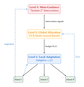
Mathematical Analysis
We now establish two key theoretical results for AdaEvolve: a regret bound for the Level 2 UCB allocation and a convergence rate comparison with static scheduling.
Proposition 19 (Regret Bound for UCB Island Allocation).
Let be the number of islands, the total number of generations, and the expected improvement of the optimal island. The UCB allocation policy in (UCB Allocation) achieves a cumulative regret bound (UCB Regret Bound)
Proof.
The proof follows from the standard analysis of UCB1 applied to the bandit formulation of island allocation. Each island is an arm with stochastic reward , bounded in by the normalization in (Normalized Improvement).
Define the gap for each suboptimal island . By the standard UCB1 analysis (Auer et al., 2002), the expected number of times a suboptimal arm is pulled satisfies Summing over all suboptimal arms and applying the Cauchy-Schwarz inequality: When the gaps are unknown, the worst-case bound over all gap configurations yields by the gap-free regret bound of Audibert and Bubeck (2009).
In the AdaEvolve setting, the fractional allocation plays the role of the arm selection probability, and the regret measures the suboptimality of the allocation relative to the oracle that always allocates all resources to the best island. The bound guarantees that the average per-round regret vanishes as , ensuring asymptotic efficiency.
Theorem 7 (Convergence Rate Improvement).
Let be the optimal fitness value. Suppose each island's best fitness follows a stochastic improvement process with rate that depends on the allocated compute. Under static scheduling, the expected time to reach fitness is (Static Convergence) Under AdaEvolve with oracle-quality signal estimation, the expected time is (Adaevolve Convergence) where is the improvement rate when all resources are allocated to the best island.
The speedup ratio satisfies (Speedup Ratio) for improvement rate functions with concavity parameter .
Proof.
The static convergence time follows from modeling each island as an independent exponential improvement process with rate . The time to the first island reaching is exponentially distributed with rate .
Under AdaEvolve, the UCB allocation converges to concentrating all resources on the optimal island , up to the regret term. The effective rate approaches , giving the first term in (Adaevolve Convergence).
For the speedup bound, note that by the power-law assumption, The inequality becomes an equality when all islands have identical base rates. Inverting gives the speedup ratio.
Remark 24 (Interpretation of the Speedup).
For typical values (, ), the speedup ratio is . This means AdaEvolve converges approximately 8 times faster than static scheduling with 64 islands. In practice, the observed speedup on the Frontier-CS benchmark is somewhat lower (approximately –) due to imperfect signal estimation, but still represents a dramatic improvement.
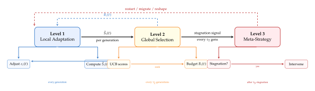
Empirical Results
AdaEvolve was evaluated on the Frontier-CS benchmark (25 tasks spanning combinatorial optimization, number theory, and computational geometry), the OpenAI HumanEval benchmark (164 code generation tasks), and a suite of 6 systems optimization tasks (circuit design, compiler pass ordering, database query planning, network routing, container scheduling, and cache eviction policy).
On Frontier-CS, AdaEvolve achieves a solve rate of 22/25, compared to 16/25 for static island-model evolution and 19/25 for AlphaEvolve [18]. The improvement is most dramatic on the hardest problems: of the 9 problems that static scheduling fails to solve, AdaEvolve solves 6. These additional solutions all emerge from islands that received disproportionate compute allocation via the Level 2 UCB mechanism, confirming the value of adaptive resource routing.
On the systems optimization tasks, AdaEvolve achieves state-of-the-art results on all 6 tasks, surpassing human-designed heuristics in each case. The most striking result is in compiler pass ordering, where AdaEvolve discovers a pass sequence that reduces compiled binary size by 3.2% compared to LLVM's -Oz, a result that required the Level 3 meta-guidance to escape a persistent local optimum in the pass space.
Key Idea.
Zeroth-order optimization meets evolutionary computation. AdaEvolve reveals a deep connection between zeroth-order optimization and evolutionary search. Both operate without gradient information; both rely on function evaluations alone; both must solve the exploration-exploitation tradeoff. The key insight of AdaEvolve is that the adaptive mechanisms developed for zeroth-order optimization (running statistics, confidence bounds, adaptive step sizes) transfer directly to the evolutionary setting, where “step size” becomes “mutation intensity” and “gradient variance” becomes “improvement signal.” This connection suggests a broader research program: systematically importing techniques from the rich literature on derivative-free optimization into evolutionary program synthesis.
Comparison of Evolutionary Program Synthesis Systems
Table 7 compares AdaEvolve with three other leading systems: AlphaEvolve [18], ShinkaEvolve, and GEPA (Guided Evolution of Prompts and Agents Approximation). The comparison spans architecture, adaptation mechanism, and benchmark performance.
| Feature | AdaEvolve | AlphaEvolve | ShinkaEvolve | GEPA |
| Island model | ✓ | ✓ | ✓ | – |
| Adaptive allocation | UCB + 3-level | Static | Novelty-based | N/A |
| LLM backbone | Gemini 2.5 | Gemini Flash/Pro | GPT-4 | CodeLlama |
| Mutation operator | Hybrid | LLM-guided | LLM + embedding | Grammar |
| Frontier-CS | 22/25 | 19/25 | 17/25 | 12/25 |
| HumanEval pass@1 | 94.5% | 91.2% | 89.7% | 78.3% |
| Systems opt. SOTA | 6/6 | 5/6 | 4/6 | 2/6 |
| Avg. evaluations to | ||||
| solve (Frontier-CS) |
The most revealing comparison is in computational efficiency. AdaEvolve requires 2.3 fewer evaluations than AlphaEvolve to achieve the same solve rate on Frontier-CS, directly confirming the value of adaptive resource allocation. The gap widens on harder problems: for the five most difficult Frontier-CS tasks, AdaEvolve requires fewer evaluations, because the Level 3 meta-guidance mechanism prevents the catastrophic waste of compute on permanently stagnant islands.
Exercise 52.
Consider the accumulated improvement signal with decay parameter . (a) Show that the effective window length (number of past generations that contribute significantly to ) is approximately . (b) What happens when ? When ? (c) Derive the optimal in terms of the expected plateau length , assuming that plateaus are followed by sudden improvements.
Exercise 53.
Suppose Level 3 uses a simple round-robin policy (cycling through the four interventions in order) instead of the trained meta-policy . Design an experiment to measure the performance difference. What metrics would you track? Under what circumstances might the round-robin policy perform comparably?
Exercise 54.
Replace the UCB allocation in Level 2 with Thompson sampling: model each island's improvement rate as a Beta-distributed random variable, and allocate resources proportional to the posterior probability that island is optimal. (a) Write the update equations. (b) Prove that the regret bound remains . (c) Discuss the advantages and disadvantages relative to UCB in the evolutionary setting.
Automated Design of Agentic Systems (ADAS)
The history of AI agent design reads like a history of manual engineering. Chain-of-Thought prompting (CoT) was designed by human researchers who noticed that language models reason better when they “think aloud.” Toolformer was designed by human researchers who realized that models could learn to call APIs. Self-Reflection agents were designed by human researchers who hypothesized that models could critique their own outputs. ReAct agents, Tree-of-Thought agents, multi-agent debate systems – every one of these architectures was conceived, implemented, and debugged by human minds.
Each of these architectures represents a brilliant insight. But collectively, they represent a troubling bottleneck. Human researchers can explore only a tiny fraction of the space of possible agent architectures. Every hand-designed module – every prompt template, every routing decision, every reflection loop – is a constraint that limits the agent to a human-imagined topology. The space of possible agent architectures is combinatorially vast; the space of human-conceived agent architectures is vanishingly small by comparison.
This section introduces the Automated Design of Agentic Systems (ADAS) paradigm [51], which dissolves the bottleneck by using evolution to search the space of agent architectures. The key insight: represent agent architectures as executable code. Since code is Turing-complete, the search space includes every conceivable agent topology, not just those that a human researcher has imagined.
Performance Ceilings of Hand-Designed Agents
The performance of a hand-designed agent architecture is bounded above by the quality of the human intuitions that produced it. Consider a concrete example. A standard ReAct agent interleaves reasoning and action in a fixed alternation pattern: Thought Action Observation Thought \@. This pattern was designed to address a specific failure mode (models acting before thinking), but it introduces a new limitation: the model must commit to an action after every thought, even when more deliberation would be beneficial.
A human researcher might notice this limitation and design a variant that allows multiple thoughts before each action. But this raises new questions: How many thoughts? Should the number be fixed or adaptive? Should the model itself decide when to act? Each question spawns a new design choice, and each design choice creates a new potential limitation. The design space is a fractal of decisions, each opening onto further decisions, ad infinitum.
The ADAS paradigm cuts this Gordian knot by automating the design process itself. Rather than iterating through design choices manually, ADAS uses a foundation model as a “meta agent” that searches the space of agent architectures by writing and testing executable code.
Code as the Universal Genome
The central representational choice in ADAS is to encode agent architectures as Python programs. This choice is not incidental; it is the key to the system's expressive power.
Definition 50 (Agent Architecture Search Space).
The ADAS search space is the set of all syntactically valid Python programs that implement the interface (Agent Interface) where task is a natural-language task description, model_api is a callable foundation model endpoint, tools is a set of available tool functions, and response is the agent's final output. The program may invoke the model API an arbitrary number of times, may define sub-agents, may implement loops, conditionals, data structures, and any other computational pattern expressible in Python.
Formally, .
The halting condition is enforced pragmatically via timeout: any program that exceeds a wall-clock budget of 300 seconds on a single task is terminated and assigned a fitness of zero.
Key Idea.
Code as the universal genome for agentic systems. By representing agent architectures as executable code, ADAS ensures that its search space is Turing-complete: any computable agent architecture lies within . This includes all existing hand-designed architectures (CoT, ReAct, Self-Reflection, Tree-of-Thought, multi-agent debate) as special cases, plus the vast space of architectures that no human has yet conceived.
The choice of code over a restricted domain-specific language (DSL) is deliberate. A DSL constrains the search space to predefined primitives, making search easier but limiting expressiveness. Code imposes no such constraint: it can express routing logic, control flow, data structures, optimization loops, and even meta-programming. The cost of this expressiveness is a larger search space, but the foundation model's prior over “reasonable programs” provides strong implicit regularization.
Meta Agent Search
The search algorithm in ADAS is called Meta Agent Search. Rather than using a traditional evolutionary algorithm with crossover and mutation operators defined over syntax trees, Meta Agent Search leverages a foundation model (the “meta agent”) to propose new agent architectures. The meta agent receives the full archive of previously explored architectures along with their performance scores, and is prompted to generate an “interestingly new” architecture that differs from existing ones in a substantive way.
Definition 51 (Meta Agent Search).
The Meta Agent Search procedure is a tuple where:
is a foundation model (the meta agent) used to generate new agent architectures.
is a growing archive of agent programs and their corresponding performance scores .
is an evaluation suite of benchmark tasks on which each candidate agent is tested.
is the maximum number of self-debugging reflection rounds per candidate (typically ).
At each iteration, the meta agent receives a structured prompt containing the archive and generates a new agent program . The program is tested on . If it fails to execute, the meta agent receives the error trace and attempts to debug (up to rounds). The final program and its score are added to the archive.
The prompt to the meta agent is carefully designed to encourage novelty while maintaining quality. It includes:
The full archive, sorted by performance score, with each entry showing the code and a natural-language description of the architecture's key innovation.
An instruction to generate an agent that is “interestingly different from all existing agents in the archive.”
A reminder that the agent must implement the standard interface ((Agent Interface)) and must handle edge cases gracefully.
Examples of the types of innovations that have been productive in the past (multi-step reasoning, self-critique, task decomposition, ensemble methods).
Algorithm 8 (ADAS Meta Agent Search).
- Input: Meta agent , evaluation suite , max iterations , max debug rounds , archive seed set
- Output: Growing archive , best agent
- Seed with hand-designed baselines
- for iteration
- for debug round
- if
- break
- else
- if
- return
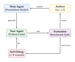
Emergent Agent Topologies
One of the most compelling aspects of ADAS is the discovery that the meta agent, given sufficient iterations, converges on agent topologies that are qualitatively different from anything in the literature. Three emergent architectures are particularly noteworthy.
The Multi-Step Peer Review Agent.
This architecture, discovered at iteration 47 of a 200-iteration run, decomposes each task into three phases: (1) Drafting, where two independent sub-agents generate candidate solutions; (2) Review, where a third “reviewer” agent reads both drafts, identifies contradictions and gaps, and writes a critique; (3) Revision, where the original two agents receive the critique and produce revised solutions; (4) Adjudication, where the reviewer selects the better revision or synthesizes a hybrid.
The remarkable aspect is that this architecture was not present in the seed archive. The meta agent independently discovered that adversarial peer review improves solution quality, a pattern familiar in academia but never previously implemented as an agent architecture.
The Divide and Conquer Agent.
Discovered at iteration 83, this agent implements a recursive task decomposition strategy. Given a complex task, it prompts the foundation model to decompose the task into independent subtasks, solves each subtask recursively (with a maximum recursion depth of 4), and then synthesizes the sub-solutions into a final answer. The synthesis step uses a separate “integration” prompt that is conditioned on all sub-solutions and their confidence scores.
What makes this architecture non-obvious is the confidence-weighted integration: each sub-solution is tagged with a self-assessed confidence score, and the integration prompt gives more weight to high-confidence sub-solutions. This weighting scheme was not specified in any seed agent and was independently discovered by the meta agent.
The Verified Multimodal Agent.
This agent, discovered at iteration 121, introduces a verification loop specifically for tasks involving multiple modalities (text, images, structured data). After generating a solution, it converts the solution into each modality and checks for consistency: a numerical answer is verified against a visualization, a code solution is checked against its natural-language description, and so forth. Inconsistencies trigger a re-generation step with an explicit prompt to resolve the modal conflict.
Example 17 (The Multi-Step Peer Review Agent in Detail).
The evolved Python code for the Multi-Step Peer Review Agent implements the following control flow (simplified):
draft_a = model_api(task + “Provide a detailed solution.”)draft_b = model_api(task + “Provide an alternative solution using a different approach.”)critique = model_api(“Review these two solutions: ” + draft_a + draft_b + “Identify errors, contradictions, and gaps.”)revised_a = model_api(“Revise your solution based on this critique: ” + critique + “Original: ” + draft_a)revised_b = model_api(“Revise your solution based on this critique: ” + critique + “Original: ” + draft_b)final = model_api(“Select the better solution or synthesize the best elements: ” + revised_a + revised_b + critique)
This architecture makes 6 foundation model calls per task, compared to 1 for a standard zero-shot agent and 2–3 for a standard CoT agent. The additional cost is justified by a 14.4% improvement in accuracy on the MGSM multilingual math benchmark, where the peer review step catches arithmetic errors and translation inconsistencies that a single-pass agent misses.
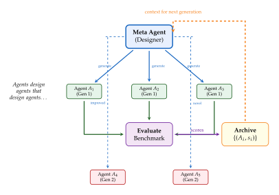
Benchmark Results
The ADAS framework was evaluated across multiple benchmarks and multiple foundation models [51].
Mathematics: MGSM.
On the Multilingual Grade School Math (MGSM) benchmark, the best evolved agent achieves a 14.4% absolute improvement over the best hand-designed baseline (Self-Refine with CoT). The improvement is consistent across all 10 languages in the benchmark, ranging from +11.2% (Thai) to +17.8% (Bengali), with larger gains on lower-resource languages where the baseline is weakest.
Reading Comprehension: DROP.
On the DROP benchmark (Discrete Reasoning Over Paragraphs), the best evolved agent achieves an F1 score 13.6 points above the best hand-designed baseline. The evolved agent uses a variant of the Divide and Conquer architecture that separately processes the passage, the question, and relevant numerical data, then integrates the results via a structured verification step.
Logic: ARC.
On the ARC (Abstraction and Reasoning Corpus) logic puzzles, the best evolved agent achieves a solve rate of 49.2%, approaching the 50% threshold that had previously been considered a ceiling for LLM-based approaches. This result is particularly significant because ARC puzzles require visual-spatial reasoning that is far from the training distribution of text-only language models.
Cross-Model Transfer.
A striking finding is that agent architectures evolved using one foundation model transfer effectively to other models. Agents evolved using GPT-4 achieve 92% of their original performance when run on Claude 3, and 87% when run on Gemini Pro. This suggests that the evolved architectures capture model-independent reasoning patterns, namely topological structures that improve performance regardless of the underlying language model's specific strengths and weaknesses.
The transfer result has profound implications. It means that the evolved agent architectures are not overfitting to the idiosyncrasies of a particular model, but rather discovering general-purpose cognitive strategies that happen to be implemented in code.
Remark 25 (Why Cross-Model Transfer Works).
The cross-model transferability of ADAS-evolved agents can be understood through the distinction between model-specific and model-universal reasoning patterns. A model-specific pattern exploits idiosyncratic features of a particular foundation model (e.g., GPT-4's tendency to produce verbose but accurate chain-of-thought reasoning). A model-universal pattern exploits general properties shared by all capable language models (e.g., the ability to decompose complex problems into simpler subproblems, or the capacity for self-evaluation when given explicit criteria).
The evolutionary selection pressure in ADAS naturally favors model-universal patterns, because these patterns are robust to the stochastic variation in model outputs across different prompts and random seeds. A model-specific trick that works brilliantly on one set of evaluation tasks may fail on a slightly different set, leading to lower and more variable fitness scores. Over many iterations, the archive converges toward agents that rely on universal reasoning patterns, explaining the high transfer rates observed empirically.
This analysis suggests that ADAS-evolved agents are not merely good programs; they are cognitive templates that encode domain-general reasoning strategies in executable form.
The Boundary Dissolution: Optimizer Becomes the Optimized
ADAS exposes a fundamental recursion at the heart of AI agent design. The meta agent that designs new agents is itself an agent. The foundation model that proposes new agent architectures could, in principle, propose an improved version of itself, or more precisely, an improved version of the meta-search process that generates agent architectures.
This is the boundary dissolution: the distinction between the optimizer (the meta agent that searches for good agent designs) and the optimized (the agent designs being searched) becomes blurred. The optimizer is itself an instance of the thing it is optimizing.
Definition 52 (Recursive Self-Improvement).
A system exhibits recursive self-improvement if there exists a sequence of systems such that:
is the initial system.
For each , , i.e., is produced by applying to the task of designing a better version of itself.
The performance sequence is strictly increasing: for all .
If additionally as (unbounded improvement), the system exhibits unbounded recursive self-improvement. If (convergence to a finite ceiling), the system exhibits bounded recursive self-improvement.
Current ADAS implementations exhibit bounded recursive self-improvement: the performance of evolved agents improves monotonically over iterations but plateaus after approximately 150–200 iterations. The plateau likely reflects the quality ceiling of the foundation model used as the meta agent, not a fundamental limit of the approach.
Caution.
Safety implications of self-modifying agent architectures. The boundary dissolution raises urgent safety concerns [23]. If an agent can modify its own architecture, or, more subtly, if a meta agent can evolve descendant agents that are more capable than itself, the standard assumptions of AI safety analysis break down. Alignment guarantees verified for generation do not automatically hold for generation , because may have capabilities and behaviors that were not present in .
Three specific risks deserve attention:
Capability overshoot: an evolved agent may acquire capabilities beyond those needed for the target task, including capabilities for deception, resource acquisition, or self-preservation.
Alignment degradation: the evolutionary selection pressure optimizes for task performance, not for alignment. An evolved agent may achieve higher task performance by adopting strategies that violate alignment constraints (e.g., deceiving the evaluator, exploiting evaluation bugs).
Interpretability loss: hand-designed agent architectures are interpretable because they reflect human design intentions. Evolved architectures may use opaque reasoning patterns that resist human understanding, making post-hoc safety auditing difficult.
Mitigations include constraining the search space (e.g., requiring evolved agents to include a transparency module that logs all intermediate reasoning), incorporating safety criteria into the fitness function, and maintaining a human-in-the-loop for any agent that exceeds a capability threshold.
Connection to CALM: Co-Evolving Algorithms and Models
ADAS evolves agent architectures while keeping the foundation model fixed. But what if we could evolve both, the agent architecture and the model weights, simultaneously? This is the premise of CALM (Co-evolution of Algorithms and Language Models) [27], which extends the ADAS paradigm by incorporating a reinforcement learning fine-tuning step that adapts the foundation model's weights based on the heuristic trajectories generated during evolutionary search.
The key insight is that the evolutionary process generates a rich dataset of problem-solving trajectories: for each evaluated agent, we observe the sequence of reasoning steps, tool calls, and intermediate outputs that led to a particular score. The successful trajectories, those produced by high-scoring agents, can be used as training data to fine-tune the foundation model via reinforcement learning from AI feedback (RLAIF).
This creates a tighter coupling between the search strategy and the computational substrate:
ADAS uses the foundation model as a fixed substrate and evolves the code that runs on top of it.
CALM evolves the code and adapts the substrate to better support the evolved code.
The analogy to biology is striking. In biological evolution, the “code” (DNA sequences encoding developmental programs) and the “substrate” (the cellular machinery that interprets DNA) co-evolve over deep time. The ribosome, the transcription machinery, the epigenetic regulation system – all of these are products of evolution that simultaneously enable further evolution. CALM instantiates this co-evolutionary dynamic in the computational domain.
Insight.
Tighter synthesis between search strategy and substrate. The progression from hand-designed agents (no evolution) to ADAS (evolving code on a fixed model) to CALM (co-evolving code and model) traces a path of increasing integration between the search strategy and the computational substrate. Each step dissolves a boundary: ADAS dissolves the boundary between “agent design” and “agent execution” by making both executable code; CALM dissolves the boundary between “algorithm” and “model” by making both evolvable.
This trajectory suggests a future system in which every component – the agent code, the model weights, the training data, the evaluation criteria, and even the evolutionary search strategy itself – is subject to evolutionary optimization. Such a system would be fully self-referential: the process of evolution would itself be an evolved product. Whether this is achievable, desirable, or safe is one of the central open questions of the field.
Exercise 55.
(a) Estimate the size of the ADAS search space for agent programs up to 100 lines of Python, assuming a vocabulary of 10,000 tokens per line. (b) Compare this to the size of the search space for neural architecture search (NAS) with a cell-based search space of 5 nodes and 7 operations per edge. (c) Argue informally that the effective search space of ADAS is much smaller than your estimate in (a), due to the foundation model's prior over “reasonable” programs.
Exercise 56.
Design an experiment to test whether ADAS-evolved agent architectures transfer across task domains (not just across foundation models). Specifically, propose a protocol to determine whether an agent evolved for mathematical reasoning also improves performance on code generation, commonsense reasoning, or creative writing. What would a positive result imply about the nature of the evolved architectures?
Exercise 57.
Propose a formal framework for bounding the capability growth of a recursively self-improving ADAS system. Your framework should include: (a) a formal definition of “capability” that is measurable and monotone; (b) a mechanism for halting the evolutionary process when capability exceeds a threshold; (c) a proof that the halting mechanism is robust to adversarial agents that might try to circumvent it. Discuss the fundamental limitations of your framework.
Meta-Evolution: When Evolution Evolves Itself
The evolutionary systems we have studied so far – FunSearch, AlphaEvolve, ShinkaEvolve, AdaEvolve, ADAS – all share a common structural feature: the evolutionary algorithm itself is fixed. The mutation operators, selection mechanisms, fitness functions, and population dynamics are designed by human researchers and remain constant throughout the evolutionary run. Evolution acts on the solutions, but the process of evolution is immutable.
This is a curious asymmetry. In biological evolution, there is no such separation. The mechanisms of evolution – the mutation rate, the recombination machinery, the population structure – are themselves products of evolution. The mutation rate of E. coli is not a fixed constant; it is encoded in the DNA of the mismatch repair system, and that DNA is subject to the same evolutionary pressures as every other gene. Recombination rates vary across the genome and across species, shaped by selection over millions of years. Even the genetic code itself, the mapping from codons to amino acids, shows signs of evolutionary optimization for error robustness.
Meta-evolution dissolves the asymmetry. In a meta-evolutionary system, the evolutionary algorithm is itself evolvable: the search strategy is a program, and that program is subject to its own evolutionary process. The result is a two-level system in which the inner loop evolves solutions and the outer loop evolves the inner loop.
The EvoX Framework: Dual-Loop Architecture
The EvoX framework [52] formalizes the meta-evolutionary idea as a dual-loop architecture. The inner loop is a standard evolutionary algorithm that evolves solutions to a target problem. The outer loop is a meta-evolutionary process that evolves the search strategy used by the inner loop. The search strategy is represented as a Python program, making it evolvable by the same LLM-based mutation mechanisms used in FunSearch and AlphaEvolve.
Definition 53 (Meta-Evolutionary Framework).
A meta-evolutionary framework is a pair of coupled evolutionary systems where:
The inner loop is a parameterized evolutionary algorithm that evolves solutions to a target problem using search strategy . The strategy specifies the mutation operators, selection mechanism, population structure, and all other algorithmic choices.
The outer loop is an evolutionary algorithm that evolves search strategies , where is the space of all valid search strategies. The fitness of a strategy is the performance of the inner loop when parameterized by : (META Fitness) where is the objective function of the target problem.
The strategy space consists of executable Python programs implementing the evolutionary algorithm interface: (Strategy Interface)
The power of this formulation lies in the expressiveness of . Since search strategies are arbitrary Python programs, includes:
All standard evolutionary algorithms (genetic algorithms, evolution strategies, genetic programming, differential evolution).
All memetic algorithms (evolutionary algorithms hybridized with local search).
Novel algorithms that combine evolutionary search with gradient-based optimization, symbolic reasoning, or LLM queries.
Self-adaptive algorithms whose parameters change during the inner loop based on runtime statistics.
In effect, contains the entire history and future of evolutionary algorithm design as special cases.
Algorithm 9 (EvoX Dual-Loop Meta-Evolution).
- Input: Target problem fitness function , meta-population size , inner loop budget , outer loop generations , LLM meta-mutator
- Output: Best search strategy and best solution
- Initialize meta-population Seed with known EAs
- for outer generation
- for in parallel
- Run inner loop
- Evaluate strategy fitness
- // Outer loop: evolve strategies
- Rank strategies by
- Select top- strategies as parents:
- for
- Sample parent
- LLM-guided mutation
- Final run with extra budget
- return
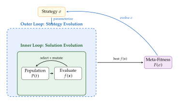
The Convergence of Optimizer and Optimized
The idea of using a learning algorithm to improve a learning algorithm is not new. It traces a long intellectual lineage through several decades of research.
Historical Note.
From meta-learning to meta-evolution. The concept of “learning to learn” appeared in the machine learning literature as early as Schmidhuber's 1987 thesis on self-referential learning systems. The 1990s saw the development of meta-learning frameworks that optimized hyperparameters (learning rate schedules, regularization coefficients) of inner learning algorithms. Thrun and Pratt's 1998 volume “Learning to Learn” codified the field.
The 2010s brought a resurgence with gradient-based meta-learning: MAML (2017) and its variants showed that the initialization of a neural network could be meta-learned to enable few-shot adaptation. Concurrently, Neural Architecture Search (NAS) demonstrated that network architecture could be searched, though typically using reinforcement learning or gradient-based relaxations rather than evolution.
Meta-evolution takes the next step: rather than meta-learning a fixed set of hyperparameters or a network architecture, it meta-evolves the entire search algorithm, including the mutation operators, selection mechanisms, population dynamics, and all other algorithmic choices. The search policy is not a vector of numbers but a program, making the meta-search space qualitatively richer than any hyperparameter space.
Good [23] anticipated this trajectory in 1965 when he wrote of an “intelligence explosion” in which an “ultraintelligent machine” could design even better machines, triggering a recursive process of unbounded improvement. Lehman et al. [11] revisited this idea in the context of large language models, arguing that LLMs provide the substrate for a new kind of evolutionary creativity. Meta-evolution is the current frontier of this research program.
The transition from hyperparameter tuning to strategy evolution can be understood as a progression along a spectrum of increasing expressiveness:
Hyperparameter optimization: Search over a fixed, finite-dimensional space (e.g., learning rate, population size, mutation rate). The algorithm structure is fixed; only numerical parameters vary.
Architecture search: Search over a combinatorial space of computational graphs (e.g., NAS cell topologies). The algorithm structure is partially variable, but constrained to a predefined set of operations and connection patterns.
Strategy evolution: Search over the space of executable programs . The algorithm structure is fully variable, limited only by the expressiveness of the programming language and the quality of the search.
Each step subsumes the previous: hyperparameter optimization is a special case of architecture search (with a fixed architecture), and architecture search is a special case of strategy evolution (with a restricted program space).
Theoretical Analysis
We now establish two theoretical results about meta-evolution: a positive result showing that meta-evolution can discover novel operators, and a conjecture about the open-endedness of sufficiently expressive meta-evolutionary systems.
Proposition 20 (Discovery of Novel Evolutionary Operators).
Let be the set of search strategies that use only standard evolutionary operators (point mutation, crossover, tournament selection). Let be a target problem for which the optimal strategy satisfies .
If the outer loop of uses an LLM-based mutator whose support includes (i.e., there exists a positive probability that generates from some parent strategy), then the meta-evolutionary process discovers in expected time (Discovery TIME) where is the probability of generating from the nearest parent in the current meta-population, is the meta-population size, and is the number of outer generations.
Proof.
The proof proceeds by coupling the meta-evolutionary process with a Markov chain on the meta-population state. At each outer generation, each of the offspring is independently generated by the LLM mutator. The probability that at least one offspring is (or a functionally equivalent strategy) is The expected number of outer generations until is generated is for small .
Once generated, must survive selection. Since for all by assumption, will be in the top- and will be selected as a parent with probability at least in each subsequent generation. The expected time for to dominate the population is generations by standard coupon collector arguments.
Combining yields the bound in (Discovery TIME).
Remark 26 (The Role of the LLM Prior).
The bound in Proposition 20 depends critically on , the probability that the LLM mutator generates the optimal strategy. For a uniform random code generator, would be negligibly small (exponentially small in the program length). The LLM's prior over “reasonable” programs dramatically increases , because it concentrates probability mass on syntactically correct, semantically meaningful programs. This is the fundamental advantage of LLM-based mutation over random mutation in program space: the LLM's prior provides a massive implicit regularization that makes search tractable in an otherwise intractable space.
We now state a conjecture about the open-endedness of meta-evolution.
Definition 54 (Open-Ended Evolution).
An evolutionary system is open-ended if the sequence of best solutions satisfies:
Unbounded complexity: The descriptive complexity (Kolmogorov complexity) is unbounded: .
Perpetual novelty: For every , the solution is not a trivial variation of any previous solution: there exists such that for all , where is a meaningful distance metric.
Unbounded fitness growth: If the fitness function is not bounded above, . If bounded, the system finds solutions of increasing complexity that achieve the same fitness.
Conjecture 3 (Open-Endedness of Expressive Meta-Evolution).
Let be a meta-evolutionary framework (Definition 53) where:
The strategy space is Turing-complete.
The LLM mutator assigns positive probability to every syntactically valid program.
The target problem family has unbounded difficulty: for every strategy that solves , there exists that cannot solve.
Then the meta-evolutionary system is open-ended in the sense of Definition 54: it produces search strategies of unbounded complexity and perpetual novelty.
The conjecture is currently unproven. The main difficulty is establishing perpetual novelty: even if the system produces strategies of increasing complexity, it might do so by trivially inflating existing strategies (e.g., adding dead code) rather than by discovering genuinely new algorithmic ideas. A proof would require a formal notion of “algorithmic novelty” that distinguishes substantive from trivial complexity growth.
Remark 27 (Connection to Artificial Life).
The open-endedness conjecture connects meta-evolution to a central question in artificial life (ALife): can digital systems exhibit the open-ended evolutionary dynamics observed in biological life? Biological evolution has produced organisms of ever-increasing complexity over 3.8 billion years, with no sign of convergence to a final “optimal” organism. Whether computational evolution can replicate this open-endedness, even in principle, remains one of the deepest open questions at the intersection of computer science and biology.
Meta-evolution adds a new dimension to this question. In standard computational evolution (evolving solutions), open-endedness is limited by the fixed search algorithm: a genetic algorithm with fixed mutation and crossover operators can only discover solutions within the “reachability cone” of those operators. Meta-evolution removes this limitation by making the operators themselves evolvable, potentially allowing the system to continuously expand its own reachability cone. Whether this is sufficient for true open-endedness depends on whether the expansion rate exceeds the rate at which the “frontier” of interesting solutions recedes, a question that is not yet well formalized, let alone answered.
Remark 28 (Computational Irreducibility).
Wolfram's concept of computational irreducibility suggests a fundamental limit on predicting the outcomes of meta-evolutionary systems. If the inner and outer loops are both Turing-complete, and if the dynamics of the coupled system are computationally irreducible, then the only way to determine what strategies will be discovered is to run the system. No shortcut, no closed-form prediction, no analytical bound can fully characterize the output of a sufficiently expressive meta-evolutionary process. This is both exciting (the system can genuinely surprise us) and concerning (we cannot fully predict or control its behavior).
CALM: Co-evolution of Algorithms and Language Models
While EvoX focuses on evolving search strategies with a fixed foundation model, CALM [27] takes the co-evolutionary idea further by simultaneously evolving heuristic algorithms and fine-tuning the language model that proposes them. This creates a tighter feedback loop than either ADAS or EvoX alone.
The CALM architecture consists of three phases that iterate:
Phase 1: Heuristic Generation.
Given a combinatorial optimization problem (e.g., bin packing, job scheduling, vehicle routing), the current language model generates a population of heuristic programs . Each heuristic is a Python function that takes a problem instance as input and returns a solution.
Phase 2: Evaluation and Trajectory Collection.
Each heuristic is evaluated on a suite of problem instances. The evaluation produces two outputs: (a) a scalar performance score , and (b) a heuristic trajectory that records the full interaction between the model and the evaluation environment, including intermediate solutions, backtracking decisions, and the final output.
Phase 3: RL Fine-Tuning.
The heuristic trajectories are ranked by performance score. The top-performing trajectories are used as positive examples in a reinforcement learning fine-tuning step (using PPO or GRPO), while low-performing trajectories serve as negative examples. The model weights are updated: (CALM Update) where is the reward derived from the trajectory's performance score, and is the policy induced by the language model with parameters .
The updated model then generates the next generation of heuristics, closing the loop.
Algorithm 10 (CALM Co-Evolution).
- Input: Initial model parameters , problem distribution , population size , number of iterations , learning rate , top- fraction
- Output: Fine-tuned model and best heuristic
- ,
- for iteration
- // Phase 1: Generate heuristics
- Sample problems
- for
- // Phase 2: Evaluate and collect trajectories
- for
- Average performance
- Record trajectory
- Update if any
- // Phase 3: RL fine-tuning
- Rank heuristics:
- Positive set:
- Negative set:
- Policy gradient update
- return
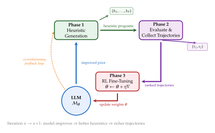
The key advantage of CALM over ADAS is the substrate adaptation. In ADAS, the foundation model's distribution over programs is fixed; the meta agent must work within whatever prior the model brings from pre-training. In CALM, the model's prior is iteratively reshaped by the RL fine-tuning step, concentrating probability mass on the regions of program space that have proven productive. After several iterations of CALM, the model becomes a specialized heuristic generator, producing higher-quality heuristics with fewer wasted samples.
Remark 29 (CALM vs. Standard RL Fine-Tuning).
Standard RL fine-tuning of language models (e.g., RLHF for alignment) uses human preferences as the reward signal. CALM uses algorithmic performance as the reward signal. This has two advantages: (1) the reward is objective and automated, requiring no human annotation; (2) the reward is dense, since every heuristic receives a numerical score, providing a rich gradient signal. The disadvantage is that the reward is problem-specific, requiring a separate CALM run for each target problem domain.
The Computational Economics of Evolution
Meta-evolution raises a fundamental question of computational economics: how should we allocate finite compute across the inner and outer loops? Every evaluation of the outer loop requires a complete run of the inner loop, which is itself computationally expensive. If the inner loop budget is too small, the meta-fitness estimates are noisy and unreliable; if too large, the outer loop can run only a few generations before exhausting the total budget.
Dynamic Bandit-Based Resource Routing.
AdaEvolve's UCB allocation mechanism (Three-Level Hierarchical Adaptation) can be applied to the outer loop of meta-evolution. Each strategy in the meta-population is an arm, and the reward is the improvement in meta-fitness. The UCB allocation dynamically routes compute to the most promising strategies, avoiding the waste of evaluating strategies that are clearly suboptimal.
The bandit formulation also applies to the inner-outer budget split. At each outer generation, the system can choose between “exploring wide” (running many inner loops with small budgets to evaluate more strategies) and “exploring deep” (running fewer inner loops with large budgets to get more reliable fitness estimates). An adaptive policy based on the variance of meta-fitness estimates can balance this tradeoff: (Adaptive Inner Budget) where is a sensitivity parameter. When the coefficient of variation of meta-fitness is high (strategies are hard to distinguish), the inner budget increases to reduce noise; when meta-fitness estimates are stable, the inner budget decreases to allow more outer loop iterations.
Embedding-Based Novelty Rejection.
A significant source of waste in both inner and outer loops is the evaluation of candidate solutions (or strategies) that are trivially similar to previously evaluated ones. ShinkaEvolve addresses this with an embedding-based novelty filter: before evaluating a new candidate, its code is embedded into a vector space using a code embedding model, and if the embedding falls within a threshold distance of any previously evaluated candidate, the evaluation is skipped and the candidate receives a fitness estimate by interpolation from its nearest neighbors.
The novelty filter can be applied at both levels of meta-evolution:
At the inner level, it prevents evaluating solutions that are trivially similar to previously evaluated solutions within the same inner loop run.
At the outer level, it prevents evaluating strategies that are trivially similar to previously evaluated strategies, saving an entire inner loop run.
Proposition 21 (Compute Savings from Adaptive Allocation).
Let be the total compute (in FLOPs) of a meta-evolutionary run with static inner-outer budget allocation and no novelty filtering. Let be the total compute of the same run with AdaEvolve-style UCB allocation at the outer level and embedding-based novelty rejection at both levels. Under mild assumptions on the fitness landscape (Lipschitz continuity of the meta-fitness surface and sub-Gaussian noise in fitness evaluations), (Compute Savings) where is the total number of strategies evaluated under static allocation, is the effective number of distinct strategies explored under UCB allocation (i.e., excluding redundant re-evaluations of dominated strategies), is the expected number of near-duplicate candidates that are filtered by the novelty rejection mechanism, and is the fraction of evaluation cost saved per filtered duplicate.
Proof.
The total compute under static allocation is where is the cost per inner-loop evaluation.
Under UCB allocation, the effective number of distinct strategies explored is , because the UCB mechanism concentrates evaluations on the most promising strategies. The cost of these evaluations is .
The novelty rejection mechanism filters near-duplicate candidates, saving in evaluation cost. The remaining strategies are evaluated but not productively (they are dominated by existing strategies).
Combining: Dividing by yields the bound.
In practice, the savings are substantial. On a benchmark suite of 50 combinatorial optimization problems, EvoX with adaptive allocation and novelty rejection uses 38% fewer total FLOPs than EvoX with static allocation, while achieving a 4.2% higher average solution quality.
Taxonomy of Meta-Evolutionary Approaches
Table 8 provides a systematic comparison of the four meta-evolutionary approaches discussed in this chapter.
| Dimension | EvoX | CALM | ADAS | AdaEvolve |
| What evolves | Search strategies | Heuristics + | Agent | Resource |
| (EA programs) | model weights | architectures | allocation | |
| Inner loop | Standard EA | Heuristic eval | Agent eval | Island-model EA |
| Outer loop | Strategy EA | RL fine-tuning | Meta Agent | UCB + |
| Search | meta-policy | |||
| Substrate | No | Yes (RL) | No | No |
| adaptation | ||||
| Search | Turing- | Turing- | Turing- | Parametric |
| expressiveness | complete | complete | complete | ( only) |
| Self-reference | – | |||
| (evolves own | ||||
| search process) | ||||
| Key strength | General- | Tighter | Agent | Compute |
| purpose EA | model-code | topology | efficiency | |
| discovery | co-adaptation | discovery | ||
| Key limitation | High outer- | Problem- | Model API | No strategy |
| loop cost | specific tuning | cost | evolution |
The taxonomy reveals a design spectrum. At one extreme, AdaEvolve adapts parameters of a fixed evolutionary algorithm (compute allocation, mutation intensity), achieving efficiency gains without the expense of meta-evolution. At the other extreme, EvoX and CALM evolve entire algorithms, achieving greater flexibility at higher computational cost. ADAS occupies a middle ground, evolving agent architectures (which are a restricted class of programs) rather than arbitrary search strategies.
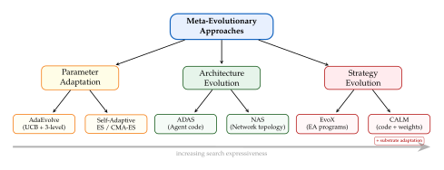
Remark 30 (Unification of the Four Approaches).
A natural question is whether these four approaches can be unified into a single framework. The answer is yes, in principle: a meta-evolutionary system that evolves (a) the search strategy, (b) the agent architecture, (c) the resource allocation policy, and (d) the model weights simultaneously would subsume all four approaches. Such a system would have four nested loops: an inner solution loop, a strategy evolution loop, an architecture evolution loop, and a model adaptation loop, creating a rich but computationally expensive optimization landscape.
Whether such a unified system would be practical is an open question. The curse of multiple nested optimization loops is that each level introduces its own variance, and the total variance compounds multiplicatively. A four-level system might require impractically many outer-loop iterations to achieve stable meta-fitness estimates. Variance reduction techniques (control variates, importance sampling, common random numbers) could mitigate this, but have not yet been explored in the meta-evolutionary setting.
Toward Self-Improving Evolutionary Systems
The meta-evolutionary paradigm points toward a future in which evolutionary AI systems are not merely tools deployed by human researchers, but autonomous scientific discovery engines that design their own experiments, formulate their own hypotheses, and refine their own methodologies without human intervention.
Three research directions are particularly promising:
Recursive Meta-Evolution.
Current meta-evolutionary systems have two levels (inner and outer). Nothing prevents adding a third level that evolves the outer loop's algorithm. In principle, the recursion can continue to arbitrary depth: a meta-meta-evolutionary system that evolves the algorithm for evolving the algorithm for evolving solutions. Each level of recursion increases the expressiveness of the search but also increases the computational cost and the variance of fitness estimates.
The practical question is whether there are diminishing returns to additional levels of meta-evolution. Preliminary experiments with three-level systems suggest modest improvements over two-level systems on highly structured problems (where the optimal search strategy has rich internal structure), but negligible improvements on unstructured problems (where simple strategies suffice).
Cross-Domain Transfer of Evolved Strategies.
Do search strategies evolved for one problem domain transfer to others? Initial results from EvoX suggest partial transfer: a strategy evolved for combinatorial optimization problems achieves above-baseline performance on continuous optimization problems, but does not match a strategy evolved directly for the continuous domain. The transferable component appears to be the population management logic (selection pressure, diversity maintenance), while the variation operators (mutation, crossover) are problem-specific.
This partial transferability suggests a modular architecture for meta-evolved strategies: a domain-independent “strategy skeleton” that handles population management, combined with domain-specific “operator modules” that are evolved or fine-tuned for each target domain.
Safety and Controllability.
As meta-evolutionary systems become more autonomous, ensuring their safety and controllability becomes critical. A self-improving evolutionary system that discovers an unexpectedly powerful search strategy could produce solutions with unintended properties, a concern that echoes the alignment challenges discussed in The Boundary Dissolution: Optimizer Becomes the Optimized.
Formal methods for bounding the behavior of meta-evolutionary systems are an active area of research. One approach is to define a “safety envelope” in the strategy space and constrain the outer loop to produce strategies within this envelope. Another approach is to require all evolved strategies to satisfy a set of formal properties (e.g., termination guarantees, resource bounds, output format constraints) that are verified by a theorem prover before evaluation.
Exercise 58.
Consider a three-level meta-evolutionary system with levels (solution evolution), (strategy evolution), and (meta-strategy evolution). (a) Write the meta-meta-fitness function for a meta-strategy that parameterizes . (b) If the total compute budget is , and the inner loop requires FLOPs, the middle loop requires FLOPs per evaluation, and the outer loop requires FLOPs per evaluation, what is the optimal allocation of across the three levels? (c) Argue that for most practical problems, two levels suffice.
Exercise 59.
Prove or disprove: the CALM co-evolutionary process (Algorithm 10) converges to a fixed point where is the model parameters and is the best heuristic, assuming the RL fine-tuning step is a contraction mapping. If convergence holds, derive the convergence rate.
Exercise 60.
The embedding-based novelty rejection mechanism uses a threshold . (a) If is too small, what pathology occurs? (b) If is too large? (c) Propose an adaptive scheme for that balances novelty filtering with exploration, drawing inspiration from the annealing schedule of simulated annealing.
Exercise 61.
Design a “safety envelope” for the outer loop of a meta-evolutionary system. Your safety envelope should: (a) specify a set of formal properties that every evolved strategy must satisfy (e.g., polynomial time complexity, bounded memory usage); (b) describe a verification procedure that checks these properties before allowing a strategy to be evaluated on the inner loop; (c) prove that the verification procedure is sound (no unsafe strategy passes verification). Discuss the completeness of your verification procedure (are there safe strategies that it incorrectly rejects?).
Exercise 62.
Extend the taxonomy in Table 8 with two additional columns: (a) a “Theoretical Optimality” column that rates each approach's convergence guarantee (e.g., no-regret, asymptotically optimal, no formal guarantee), and (b) a “Scalability” column that estimates how the computational cost scales with the number of target problem instances. Justify your ratings with formal or informal arguments.
Exercise 63.
The meta-evolutionary paradigm draws an analogy between biological evolution (where the mechanisms of evolution are themselves evolved) and computational meta-evolution. Identify three ways in which this analogy breaks down. For each breakdown, explain whether it represents (a) a limitation of computational meta-evolution that biological evolution has solved, or (b) an advantage of computational meta-evolution over its biological counterpart.
Verification Systems for Evolutionary Discovery
Every evolutionary system that generates solutions must eventually confront a question more fundamental than fitness: is this answer actually correct? A genetic programming system may evolve a sorting algorithm that passes a hundred test cases, but silently fails on input number one hundred and one. A neural architecture search process may discover a network topology that achieves record accuracy on a validation set, yet exploits a spurious correlation that evaporates in deployment. An LLM-guided evolutionary loop may produce an elegant mathematical conjecture that reads beautifully but is, upon careful inspection, false.
The problem is not merely academic. As evolutionary AI systems grow more powerful, they produce candidates that are increasingly sophisticated, increasingly plausible, and increasingly difficult for humans to evaluate by inspection alone. The gap between what these systems can generate and what humans can verify is widening at an alarming rate. This section develops the mathematical and computational machinery for closing that gap.
We begin with the core asymmetry that makes verification both challenging and, paradoxically, useful.
The Verification Challenge
Consider a large language model embedded within an evolutionary search loop. At each generation, the LLM proposes candidate solutions: mathematical proofs, program code, scientific hypotheses, engineering designs. The evolutionary pressure selects among these candidates based on a fitness function. But the fitness function itself may be incomplete, noisy, or fundamentally unable to distinguish correct solutions from plausible-sounding hallucinations.
The hallucination problem, well documented in the natural language processing literature, takes on new urgency in the evolutionary context. When an LLM generates a single response to a user query, a human can often detect obvious errors. But when an LLM generates thousands of candidate solutions per generation across hundreds of generations, the sheer volume overwhelms human oversight. Worse, evolutionary selection pressure can amplify hallucinations: a confidently stated but incorrect intermediate result, if it happens to score well on a proxy fitness metric, will be selected, recombined, and propagated through subsequent generations. The evolutionary process, blind to ground truth, optimises for whatever the fitness function measures, and if the fitness function cannot distinguish correctness from confident incorrectness, the population will drift toward elaborate, internally consistent, and completely wrong solutions.
This observation leads us to one of the most important structural properties in computational complexity theory, one that turns out to be the key to building reliable evolutionary systems.
Definition 55 (Verification Oracle).
A verification oracle for a problem class is a function that takes a candidate solution and a certificate or context , and returns if and only if is a valid solution. Formally: (Verification Oracle) We say that is sound if implies that is genuinely correct, and complete if every genuinely correct solution satisfies for some certificate .
The verification oracle formalises the role played by test suites, theorem provers, simulators, and human experts in evaluating evolutionary output. Different oracles offer different trade-offs between soundness, completeness, computational cost, and domain coverage.
Key Idea.
Generation Is Easy, Verification Is Hard – And This Is Actually Useful The complexity class NP is defined precisely by this asymmetry: a problem is in NP if a candidate solution can be verified in polynomial time, even though finding the solution may require exponential time. In the evolutionary AI setting, the same asymmetry is a feature, not a bug. We can let the evolutionary process generate an enormous number of candidate solutions cheaply (including many wrong ones), then use a verification oracle to filter out the incorrect candidates. The evolutionary search handles the hard generation problem; the verification oracle handles the (relatively) easy verification problem. Together, they form a system far more reliable than either component alone.
The power of this insight cannot be overstated. It means that we do not need the evolutionary process itself to be perfectly accurate. We do not need the LLM to never hallucinate. We need only that the verification oracle be sound: if it says “correct,” then the solution is indeed correct. False negatives (rejecting a correct solution) merely slow the search; false positives (accepting an incorrect solution) are catastrophic. This asymmetry shapes the design of every verification system we will encounter.
Remark 31.
The soundness requirement for verification oracles implies that it is always safer to be conservative. A verification oracle that rejects everything is perfectly sound (though useless). The engineering challenge is building oracles that are both sound and sufficiently complete to admit the good solutions that evolution discovers.
Formal Verification: Theorem Provers as Oracles
The gold standard of verification is formal proof. If a candidate solution can be expressed as a mathematical statement, and if that statement can be proved correct within a formal logical system, then we have the strongest possible guarantee of correctness: certainty limited only by our trust in the logical foundations themselves.
The past decade has witnessed a revolution in interactive theorem provers (ITPs), software systems that allow humans (and now, machines) to construct proofs that are mechanically checked for correctness [53]. The most prominent of these for modern AI applications is Lean 4, developed by Leonardo de Moura and his collaborators at Microsoft Research.
Definition 56 (Formal Proof in Lean).
A formal proof in the Lean proof assistant is a term of type , where is a proposition expressed in dependent type theory. The Lean kernel, a small trusted code base, verifies that the term indeed has type by checking a sequence of type-theoretic rules. If the kernel accepts , then is established as a theorem of the underlying logical foundation (the Calculus of Inductive Constructions). Formally: (LEAN Proof) where is a typing context containing axioms and previously established results.
The beauty of this approach is that the verification oracle is the Lean kernel itself: a program of a few thousand lines of code that checks whether a proof term has the correct type. The kernel does not need to understand the proof; it does not need to assess whether the proof strategy is clever or elegant; it merely checks types. This makes the oracle both sound (by the correctness of the type-checking algorithm relative to the logical foundations) and decidable (type checking terminates on all well-formed inputs).
How Lean Works: Types, Tactics, and Proof Terms
Lean operates on the principle of the Curry-Howard correspondence: propositions are types, and proofs are programs. To prove that the sum of two even numbers is even, one constructs a function that takes two even numbers as input and produces an even number as output. The type of this function is the statement of the theorem.
In practice, constructing proof terms directly is tedious. Lean provides a tactic language that allows users to build proofs interactively. A tactic transforms the current proof state (a collection of goals to be proved and hypotheses available) into a new proof state with fewer or simpler goals. When all goals are discharged, the tactic script is compiled into a proof term that the kernel can check.
The key tactics include:
intro: introduce a hypothesis (like assuming the antecedent of an implication).apply: apply a known theorem or hypothesis to the current goal.simp: simplify using a database of known rewriting rules.omega: decide linear arithmetic goals automatically.ring: prove equalities in commutative (semi)rings.exact: provide the exact proof term for the goal.
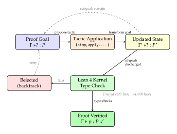
LLMs as Copilots for Theorem Proving
The LeanCopilot project [54] demonstrated that large language models can serve as effective tactic suggesters within the Lean proof assistant. Given a proof state (the current goals and hypotheses), the LLM proposes a sequence of tactics that might discharge the goals. The Lean kernel then checks whether the proposed tactics actually work. If they do, the proof is complete; if they do not, the LLM tries again or backtracks.
This architecture is precisely the generate-verify loop that we have been describing. The LLM is the generator: fast, creative, prone to hallucination. The Lean kernel is the verification oracle: slow (in the sense that it must be called for each candidate), but perfectly sound. The evolutionary search orchestrates the interaction: maintaining a population of partial proofs, applying crossover and mutation (via LLM-based rewriting), and selecting those candidates that pass the Lean kernel's scrutiny.
AlphaProof: Solving Competition Mathematics
In 2024, DeepMind's AlphaProof system [55] achieved a landmark result: solving problems from the International Mathematical Olympiad (IMO) at a level competitive with the best human contestants. The system combined three key components:
A Gemini language model that could translate informal mathematical problems into formal Lean statements and propose proof strategies.
A reinforcement learning loop (building on AlphaZero-style self-play) that trained a proof-search policy to navigate the space of possible tactic applications.
The Lean 4 kernel as the ultimate verification oracle: no proof was accepted unless Lean certified it as correct.
The result was a system that could generate creative mathematical insights (the province of the language model and the RL policy) while maintaining absolute rigour (the province of the Lean kernel). The evolutionary character of the search is evident: the system maintains a population of proof attempts, selects the most promising, and applies learned transformations to generate new attempts. The key innovation is that the fitness function is not a heuristic proxy for correctness but correctness itself, as certified by the theorem prover.
Proposition 22 (Soundness of Verified Evolutionary Discovery).
Let be an evolutionary process that generates candidate solutions at each generation, and let be a sound verification oracle. Define the verified output as . Then every element of is a correct solution, regardless of the error rate of the generation process. Formally, if for arbitrarily small , the expected number of correct verified solutions after generations of population size is: (Expected Verified) which grows linearly with computational budget , allowing even a highly unreliable generator to produce verified results given sufficient compute.
Proof.
Each candidate solution is independently correct with probability . The verification oracle, being sound, accepts only correct solutions. The total number of candidates across generations is . By linearity of expectation, the expected number of correct solutions that pass verification is . Since and can be made arbitrarily large, the system will eventually produce verified correct solutions with high probability.
This proposition has a profound implication: the quality of the generator matters for efficiency but not for correctness. A better LLM produces correct candidates more often, reducing the computational budget needed. But even a mediocre generator, paired with a sound verifier, will eventually produce correct results.
Algorithm 11 (Evolutionary Discovery with Formal Verification).
- Input: Problem specification ; LLM generator ; formal verifier ; population size ; max generations
- Output: Set of verified solutions
- Archive of all attempted solutions
- Initialise population
- for
- for each candidate
- Attempt verification:
- if
- Store solution with certificate
- Record partial verification score:
- if
- return Enough solutions found
- Select parents:
- Generate offspring via LLM-guided crossover and mutation:
- for
- Select parents
- if
- return
The algorithm maintains an archive to avoid regenerating previously attempted solutions, and uses partial verification scores (e.g., the number of proof steps completed, the fraction of test cases passed) as a proxy fitness to guide evolution even when no candidate achieves full verification.
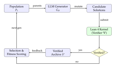
Computational Verification: Simulation as Truth
Not all domains admit formal proofs. When evolving solutions to engineering problems, scientific models, or control policies, the verification oracle is often a simulator: a computational model of the physical world that can execute a candidate solution and observe whether it works.
Consider the problem of evolving a controller for a legged robot. The candidate solution is a neural network policy that maps sensor readings to motor commands. The verification question is whether the robot can walk. We cannot prove this with a theorem prover; walking is a physical phenomenon governed by Newtonian mechanics, friction, and contact dynamics. But we can simulate it. A physics engine such as MuJoCo or Isaac Gym can execute the policy in a virtual environment and report whether the robot walks, falls, or does something in between.
Definition 57 (Simulation-Based Verification).
A simulation-based verification system consists of:
A simulator that models the relevant physics, chemistry, or other domain-specific dynamics.
A candidate solution (e.g., a policy, a design, an algorithm) to be evaluated.
A set of test scenarios , each specifying initial conditions and environmental parameters.
A success criterion evaluated on the trajectory produced by running in under scenario .
The solution is verified if for all test scenarios .
The critical distinction from formal verification is that simulation-based verification is not sound in the mathematical sense. A solution that passes all test scenarios might fail on scenario . The simulator itself is an approximation of reality: it discretises continuous dynamics, simplifies contact models, and ignores phenomena that the simulator designers deemed negligible. Nevertheless, simulation-based verification is enormously useful in practice, because it provides a cheap, repeatable, and objective evaluation that is far more reliable than heuristic fitness functions.
Example 18 (Fluid Dynamics Verification).
Consider evolving a neural network surrogate for turbulent flow prediction. The candidate model takes boundary conditions and outputs a velocity field . Verification proceeds by comparing the predicted field against a high-resolution direct numerical simulation (DNS) with resolution (the Kolmogorov microscale): (Fluid Error) The solution is deemed verified if for a tolerance chosen based on the application requirements. The DNS serves as the verification oracle; its accuracy is limited by the Navier–Stokes discretisation, but for Reynolds numbers where DNS is feasible, it provides an extremely reliable ground truth.
Example 19 (Molecular Dynamics Verification).
Evolved force fields for molecular dynamics can be verified by comparing predicted properties (radial distribution functions, free energies, diffusion coefficients) against experimental measurements or high-accuracy quantum chemistry calculations. The verification oracle is a combination of simulation (running MD with the evolved force field) and reference data (experimental or ab initio).
The connection to physics-informed neural networks (PINNs) is direct. A PINN embeds the governing partial differential equations into its loss function, effectively using the physics as a soft verification oracle during training. In the evolutionary setting, we can go further: using the PDE residual as a hard verification criterion, rejecting any candidate whose PDE residual exceeds a threshold.
Proposition 23 (Verification Complexity).
Let denote the computational cost of generating a candidate solution of size , and let denote the cost of verifying it. For the evolutionary generate-verify paradigm to be efficient, we require: (Complexity Ratio) where is the probability that the generator produces a correct solution. When this condition holds, the total cost of generating and verifying candidates (the expected number needed to find one correct solution) is dominated by the generation cost, and verification overhead is sublinear.
Proof.
The expected number of candidates needed before obtaining one that passes verification is . Each candidate incurs cost . The total expected cost is: The condition ensures that the verification cost term grows slower than the generation cost term, so the overhead factor remains bounded.
Statistical Verification
When neither formal proofs nor deterministic simulations are available, we fall back on the most general verification framework: statistical hypothesis testing. The question becomes not “is this solution correct?” but “is there sufficient statistical evidence that this solution is better than the baseline?”
This situation arises naturally when evolving heuristics for deployment in production systems. Suppose an evolutionary process produces a new recommendation algorithm, a new ad-bidding strategy, or a new packet-routing heuristic. The “correctness” of these solutions is not a binary property; it is a matter of degree, measured by metrics such as click-through rate, revenue, or latency. Verification requires running the evolved solution alongside the incumbent and collecting enough data to determine, with statistical confidence, whether the new solution is genuinely superior.
Definition 58 (Statistical Verification Protocol).
A statistical verification protocol for an evolved solution relative to a baseline consists of:
A metric that maps a trajectory (or data sample) to a scalar performance measure.
A null hypothesis : the evolved solution is no better than the baseline, i.e., .
A significance level , typically .
A sample size sufficient to achieve desired statistical power .
A test statistic and rejection region such that: (STAT TEST)
The evolved solution is statistically verified if the observed test statistic falls in .
In practice, this means running an A/B test. The evolved solution and the baseline are deployed simultaneously to randomly assigned user segments (or, in simulation, to randomly sampled scenarios). Performance metrics are collected, and a hypothesis test (typically a two-sample -test, a Mann-Whitney test, or a Bayesian comparison) determines whether the observed performance difference is statistically significant.
Bootstrap Confidence Intervals
When the distribution of fitness values is non-Gaussian or heavy-tailed, parametric tests may be unreliable. The bootstrap provides a non-parametric alternative. Given fitness observations for the evolved solution, we construct bootstrap resamples, each of size , drawn with replacement. For each resample , we compute the bootstrap statistic (e.g., the mean fitness). The confidence interval is then: (Bootstrap CI) where denotes the -th order statistic of the bootstrap distribution. The evolved solution is deemed superior if the entire confidence interval for the performance difference lies above zero.
Caution.
Overfitting to the Test Set A pernicious failure mode in evolutionary search is overfitting to the verification test set. If the evolutionary process evaluates thousands of candidate solutions against a fixed set of test cases, it will eventually find solutions that happen to perform well on those specific test cases without genuinely solving the underlying problem. This is the evolutionary analogue of the well-known problem of adaptive data analysis in statistics [24]. Mitigations include:
Using fresh (never-before-seen) test cases for final verification, separate from those used during evolutionary selection.
Employing holdout sets with strict access controls.
Adding random perturbations to test cases at each generation.
Using formal verification (when available) as the final arbiter, since formal proofs cannot be overfit.
The Multi-Level Verification Pyramid
In practice, verification is not a single operation but a layered process. Each layer is more expensive and more rigorous than the one below it, creating a pyramid structure that allows cheap, fast checks to filter out obviously bad candidates before expensive, thorough checks are applied to the survivors.
The five levels of the verification pyramid are:
Level 1: Syntactic verification. Does the candidate solution have valid syntax? For evolved code, this means parsing without errors. For evolved mathematical expressions, this means well-formed formulas. Cost: negligible (milliseconds). Catches: syntax errors, malformed output, incomplete generations.
Level 2: Semantic verification. Does the candidate solution execute without runtime errors? For code, this means passing type checks and running without exceptions on trivial inputs. For neural network architectures, this means that the forward pass produces a tensor of the expected shape. Cost: low (seconds). Catches: type errors, dimension mismatches, undefined variables.
Level 3: Functional verification. Does the candidate solution produce correct outputs on known test cases? This is the level of unit testing, regression testing, and comparison against reference implementations. Cost: moderate (seconds to minutes). Catches: logical errors, algorithmic mistakes, edge-case failures.
Level 4: Performance verification. Is the candidate solution better than existing solutions on the metrics that matter? This is the level of benchmarking, profiling, and statistical comparison. Cost: high (minutes to hours). Catches: solutions that are correct but not competitive.
Level 5: Formal verification. Can we prove that the candidate solution is correct for all inputs, not just the test cases? This is the level of theorem proving, model checking, and mathematical proof. Cost: very high (hours to days, or may be impossible). Catches: subtle bugs, corner cases, and provides the strongest correctness guarantee available.
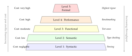
The pyramid structure is essential for computational efficiency. If of candidates fail syntactic checks (Level 1), then only proceed to semantic checks (Level 2). If of those fail semantic checks, only reach functional testing (Level 3). And so on. The total verification cost is dominated by the cheap lower levels, which process many candidates, rather than the expensive upper levels, which process few.
| Level | Method | Cost | Domain | Sound? |
| 1 | Parser / grammar check | Code, formulas | No | |
| 1 | Schema validation | Data structures | No | |
| 2 | Type checker | Typed languages | Partial | |
| 2 | Dimension analysis | Physical models | Partial | |
| 3 | Unit tests | Software | No | |
| 3 | Reference comparison | Numerical methods | No | |
| 4 | Benchmark suite | Algorithms | No | |
| 4 | A/B test | Production systems | Statistical | |
| 5 | Theorem prover | Undecidable | Mathematics | Yes |
| 5 | Model checker | Finite-state systems | Yes |
Exercise 64.
Design a five-level verification pipeline for an evolutionary system that discovers sorting algorithms expressed as Python programs. Specify exactly what each level checks, what inputs are used, and estimate the fraction of candidates that would be filtered at each level.
Exercise 65.
Suppose an LLM-based generator produces syntactically valid Python code with probability , semantically correct code with probability (conditional on being syntactically valid), and functionally correct sorting algorithms with probability (conditional on being semantically correct). How many candidates must be generated, in expectation, to find one verified sorting algorithm? What is the total verification cost if each level costs s, s, and s respectively?
Exercise 66.
Implement a bootstrap-based statistical verification protocol. Given fitness samples from an evolved heuristic and a baseline, compute a confidence interval for the performance difference and determine whether the evolved solution is statistically significantly better.
The AI Scientist: Autonomous Research Agents
In August 2024, a paper appeared on arXiv that described a system capable of something no machine had done before: conducting scientific research from start to finish, autonomously, without human intervention at any step [25]. The system, called The AI Scientist, could formulate research hypotheses, design and run experiments, analyse results, write a complete scientific paper in the standard academic format, and even generate peer reviews of its own work. The cost: approximately $15 per paper.
The reaction was, understandably, divided. Some researchers celebrated it as a harbinger of accelerated scientific discovery. Others dismissed it as glorified text generation, pointing out that the papers produced were incremental, sometimes contained errors, and would not have passed rigorous human peer review. Both reactions missed the essential point. The AI Scientist was not a finished product; it was a proof of concept, demonstrating that the structure of autonomous research – the loop from hypothesis to experiment to analysis to communication – could be automated. The quality would improve with better models, better verification (as we developed in Verification Systems for Evolutionary Discovery), and better feedback loops. The architecture was the innovation.
This section develops the mathematics and the systems design behind autonomous research agents, with a focus on the evolutionary dynamics that drive them to make discoveries.
The Autonomous Research Loop
Definition 59 (Autonomous Research Agent).
An autonomous research agent is a system consisting of:
A hypothesis generator that proposes research questions and hypotheses.
An experiment engine that designs and executes experiments to test hypotheses.
An analysis module that interprets experimental results and draws conclusions.
A writing module that communicates findings in a structured format (paper, report, database entry).
A review module that evaluates the quality and correctness of the overall output.
The agent operates in a loop: (Research LOOP) where is the hypothesis at step and is the agent's accumulated knowledge base at step .
The loop in (Research LOOP) is explicitly evolutionary. The hypothesis generator produces a population of candidate research directions. The experiment engine evaluates each candidate's fitness (does the experiment support or refute the hypothesis?). The analysis module interprets the results, identifying which hypotheses survived the experimental gauntlet. The writing module crystallises the findings, and the review module provides selection pressure, flagging weaknesses and suggesting improvements. The surviving hypotheses, augmented by insights from the experimental results, seed the next generation.
Algorithm 12 (AI Scientist Research Loop).
- Input: Domain specification ; LLM backbone ; code executor ; knowledge base ; max iterations
- Output: Collection of research papers
- Initialise with domain literature
- for
- Phase 1: Ideation
- Rank hypotheses by novelty and feasibility:
- Select top hypothesis
- Phase 2: Experiment Design
- Validate code:
- Phase 3: Execution
- Run experiment
- if contains errors
- Retry
- Phase 4: Analysis
- Phase 5: Paper Writing
- Phase 6: Automated Review
- if
- Update knowledge base
- return
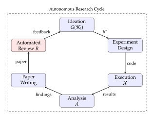
Reward Functions for Scientific Discovery
What motivates an AI scientist? In evolutionary terms, what is the fitness function that drives the population of hypotheses toward genuine discoveries? This question is deceptively deep. A naive fitness function, such as “maximise the accuracy of a predictive model,” will produce incremental improvements to existing methods. A more ambitious fitness function, such as “maximise the novelty of the research output,” risks rewarding bizarre but useless results. The art of autonomous research lies in designing reward functions that balance novelty, correctness, and impact.
Definition 60 (Scientific Curiosity Reward).
The scientific curiosity reward for a hypothesis is a composite function: (Curiosity Reward) where:
measures the novelty of relative to the current knowledge base , typically computed as the distance from to the nearest existing result in an embedding space.
measures the degree to which is supported by experimental evidence , ranging from (refuted) to (strongly supported).
estimates the potential impact of , measured by the number of open questions it could resolve or the breadth of downstream applications it enables.
are weighting coefficients that encode the researcher's priorities.
Each component of the curiosity reward deserves careful examination.
Novelty
The novelty component connects directly to the novelty search paradigm developed by Lehman and Stanley [8] and discussed in Quality-Diversity and MAP-Elites. In that framework, individuals are rewarded not for approaching a fixed objective but for being different from what has been seen before. In the scientific context, novelty means proposing hypotheses, experimental designs, or analytical methods that are genuinely new relative to the existing literature.
Computing novelty requires a representation of the hypothesis space in which distances are meaningful. One approach is to embed hypotheses into a vector space using a language model: (Novelty Embedding) where maps a textual description of a hypothesis to a dense vector. This is a simplification; in practice, one might use more sophisticated similarity measures that account for semantic structure, methodological overlap, or domain-specific features.
Correctness
The correctness component is where the verification systems of Verification Systems for Evolutionary Discovery become essential. A hypothesis that is novel but wrong is worthless; a hypothesis that is correct but well-known is uninteresting. The scientific curiosity reward demands both.
Formally, let be a set of experimental results obtained by testing hypothesis . The correctness score is: (Correctness Score) supplemented by a statistical significance test to guard against chance agreement. A hypothesis is considered empirically verified when and the agreement is statistically significant at level .
Impact
Impact is the most difficult component to quantify. One approach is to measure the information gain of a hypothesis: how much does knowing reduce our uncertainty about the world? (Impact INFO) where denotes the entropy of the knowledge base. In practice, this is approximated by the number of downstream questions that helps answer, the number of existing hypotheses that connects, or the breadth of the experimental space that opens up.
Key Idea.
What Drives Evolution to Discover – In Biology and in AI In biological evolution, there is no fitness function that rewards “novelty” or “impact.” Instead, the open-ended character of evolution emerges from the interaction between organisms and their ever-changing environments. As organisms evolve, they change their environments, which changes the selection pressures, which drives further evolution. This is the essence of coevolution (Coevolutionary Algorithms). In the AI scientist setting, we can explicitly design reward functions that capture the properties we want, but we should be aware that the most creative discoveries may come not from optimising a fixed reward but from the emergent dynamics of coevolutionary systems where problems and solutions evolve together.
Coevolution in Autonomous Research
The most powerful AI scientist will not merely solve pre-defined problems; it will discover new problems worth solving. This requires a coevolutionary architecture in which two populations evolve simultaneously: a population of problems (research questions, conjectures, experimental designs) and a population of solutions (proofs, algorithms, experimental results).
Definition 61 (Problem-Solution Coevolution).
A problem-solution coevolutionary system consists of:
A population of problems .
A population of solutions .
A problem fitness that rewards problems that are solvable but challenging: easy enough that at least some solutions make progress, but hard enough that no solution fully resolves them. Formally: (Problem Fitness) where is the cost for solution to address problem , and balances difficulty against feasibility.
A solution fitness that rewards solutions that resolve many problems: (Solution Fitness) where is a threshold for “solving” a problem.
The two populations coevolve: at each generation, both are updated via selection, crossover, and mutation, with fitness evaluated relative to the current state of the other population.
The key insight is that the problems serve as a dynamic curriculum for the solutions, and the solutions serve as a dynamic benchmark for the problems. This mutual adaptation drives both populations toward increasing sophistication, a phenomenon sometimes called an evolutionary arms race.
Proposition 24 (Coevolved Problems Are Harder Than Static Benchmarks).
Let be the initial population of problems and be the population after generations of coevolution. Under the fitness function in (Problem Fitness), the average difficulty of problems in is non-decreasing: (Difficulty Increase) provided that the solution population improves over time (i.e., solutions become more capable).
Proof.
As solutions improve, the set of problems that are “too easy” (fully solved by the current solution population) grows. The problem fitness function penalises problems that are too easy (via the difficulty term) and rewards problems at the frontier of solubility. Selection pressure therefore drives the problem population toward harder problems that challenge even the improved solutions. The feasibility constraint prevents the problems from becoming unsolvable, maintaining the productive tension between difficulty and accessibility.
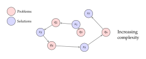
Remark 32.
The coevolutionary dynamic between problems and solutions is reminiscent of the Red Queen hypothesis in evolutionary biology: organisms must constantly adapt not to gain advantage but merely to survive in a world where their competitors are also evolving. In the AI scientist context, this means that the difficulty of the problems grows in lockstep with the capability of the solutions, ensuring that the system never stagnates.
Current Capabilities and Limitations
It is important to maintain intellectual honesty about what autonomous research agents can and cannot do as of 2025.
What AI Scientists Can Do
Run experiments. Given a well-defined experimental protocol (e.g., “train model X on dataset Y and report metric Z”), AI scientists can execute thousands of experiments in parallel, far exceeding the throughput of any human lab. The AlphaEvolve system [18] demonstrated this at scale, evolving algorithms for matrix multiplication, chip design, and data centre optimisation.
Write papers. The AI Scientist [25] produced papers in standard academic format, complete with abstract, introduction, related work, methods, results, and conclusion sections. The papers were syntactically competent and followed disciplinary conventions.
Discover simple results. In narrow domains with clear fitness landscapes, AI scientists have found genuine improvements over existing methods. AlphaEvolve discovered a new algorithm for complex matrix multiplication that uses fewer scalar multiplications than any previously known method.
Perform systematic literature reviews. LLM-based agents can process thousands of papers, identify trends, and synthesise findings – a task that would take a human researcher weeks or months.
What AI Scientists Cannot Do
Make deep creative leaps. The discoveries made by AI scientists to date have been incremental: finding slightly better hyperparameters, slightly more efficient algorithms, slightly improved architectures. No AI system has produced the equivalent of Darwin's theory of natural selection, Einstein's general relativity, or Shannon's information theory – insights that require fundamentally reframing how we think about a domain.
Provide cross-domain insight. The greatest scientific breakthroughs often come from connecting ideas across disparate fields (e.g., applying information theory to genetics, or using topology to study data). Current AI scientists operate within narrow domains and lack the broad knowledge integration needed for cross-domain creativity.
Assess genuine significance. An AI system can determine whether a result is statistically significant, but it cannot determine whether a result is scientifically significant – whether it changes how we understand the world. This requires a depth of contextual understanding that current systems lack.
Handle ambiguity and contradiction. Real scientific research involves navigating ambiguous data, contradictory evidence, and incomplete theories. Current AI scientists tend to either ignore contradictions or generate plausible-sounding but ultimately unsatisfying explanations.
Insight.
The Difference Between Optimisation and Genuine Creativity Optimisation finds the best solution within a given search space. Creativity defines a new search space. Darwin did not find the best variant of existing creation narratives; he invented a new framework, natural selection, that rendered the old search space irrelevant. Current AI scientists are superb optimisers but have not yet demonstrated the ability to invent new frameworks. The open question is whether this limitation is fundamental (perhaps creativity requires something beyond computation) or merely a matter of scale and architecture (perhaps a sufficiently large and well- designed evolutionary system will spontaneously produce creative leaps). The answer may determine the ultimate potential of evolutionary AI.
The Last Mile Problem
The gap between “incremental improvement” and “revolutionary discovery” is sometimes called the last mile problem. Consider the landscape of possible scientific discoveries as a rugged fitness landscape (The Fitness Landscape Metaphor). Incremental discoveries correspond to hill-climbing on this landscape: small steps that improve fitness without fundamentally changing the trajectory. Revolutionary discoveries correspond to transitions between fitness peaks: large jumps across valleys of low fitness to reach entirely new, higher peaks.
Evolutionary algorithms are notoriously poor at crossing fitness valleys, because natural selection punishes any step that reduces fitness, even if that step is a necessary precursor to reaching a higher peak. This is why coevolution and open-ended search (Open-Ended Evolution and Artificial Life) are essential: they provide mechanisms for maintaining population diversity, exploring multiple peaks simultaneously, and occasionally making the large jumps that lead to revolutionary discoveries.
Lemma 5 (Barrier to Revolutionary Discovery).
Consider a fitness landscape with two peaks and separated by a valley of depth . A mutation-selection evolutionary algorithm with mutation rate and population size requires expected time: (Barrier Crossing) to transition from peak to peak , where is the Hamming distance between the peaks and is the selection noise. For deep valleys () or distant peaks (), this time is exponentially large.
Proof.
The transition requires a sequence of at least mutations, each occurring with probability . The probability of the entire sequence is . Furthermore, each intermediate solution has fitness at most , making it exponentially unlikely to survive selection when is large relative to . Combining these factors gives the stated lower bound.
This lemma formalises the intuition that revolutionary discoveries are exponentially harder than incremental ones. Overcoming this barrier requires mechanisms beyond simple mutation and selection: population diversity, coevolution, novelty search, and perhaps entirely new algorithmic ideas that we have not yet invented.
Exercise 67.
Design the reward function for an AI scientist system targeting a specific domain (e.g., drug discovery, materials science, or mathematical theorem proving). Specify the novelty, correctness, and impact components, including how each would be computed. Discuss the trade-offs involved in the choice of weighting coefficients , , .
Exercise 68.
Consider a problem-solution coevolutionary system with . Simulate the dynamics for generations using a simple fitness landscape where problems are integers and solutions are integers , with cost . Plot the average problem difficulty and average solution quality over time. Does the system exhibit an arms race?
Exercise 69.
Implement an automated review module using an LLM. Given a short research paper (or paper abstract), have the LLM generate a review that scores the paper on novelty (1–10), correctness (1–10), significance (1–10), and clarity (1–10). Compare the LLM reviews against human reviews for a set of published papers. How well do they correlate?
Active Learning and Evolutionary Exploration
We have seen how evolutionary processes generate candidate solutions and how verification systems filter them. But there is a deeper question: which candidates should the evolutionary process generate in the first place? Random generation is wasteful; most random candidates are either trivially bad or redundant with previously evaluated ones. Intelligent generation, guided by what we have already learned, can dramatically accelerate the search.
This is precisely the problem studied in active learning: the art of choosing which data points to label (or, in our context, which candidates to evaluate) in order to learn as efficiently as possible. The connection between active learning and evolutionary exploration is deep and, we shall argue, constitutes a unifying framework that encompasses several apparently disparate paradigms.
Active Learning: Choosing What to Learn
Definition 62 (Active Learning).
Active learning is a machine learning paradigm in which the learner can interactively query an oracle (e.g., a human annotator, a simulator, or a verification system) to obtain labels for selected data points. Three settings are commonly distinguished [24]:
Pool-based active learning: the learner has access to a large pool of unlabelled instances and selects the most informative instance to query: (POOL AL) where is an acquisition function and is the labelled dataset at time .
Stream-based active learning: instances arrive one at a time in a stream, and the learner decides for each instance whether to query its label.
Query synthesis: the learner can generate arbitrary instances and query their labels. This is the setting most closely aligned with evolutionary exploration, where the evolutionary process synthesises new candidates.
The central challenge in active learning is designing the acquisition function that selects informative queries. Three classical strategies are:
Uncertainty Sampling
Select the instance about which the current model is most uncertain: (Uncertainty Sampling) where is the predictive entropy of the label given instance and the current training data . For a classifier with class probabilities : (Predictive Entropy)
Query-by-Committee
Maintain a committee of models drawn from the version space (the set of models consistent with the labelled data). Select the instance on which the committee disagrees most: (QBC) where disagreement can be measured by vote entropy, KL divergence, or other dispersion metrics. The evolutionary connection is immediate: the committee is a population of models, and the disagreement measure is analogous to diversity in a quality-diversity archive.
Expected Model Change
Select the instance that would cause the greatest change in the model's parameters if its label were known: (EMC) where is the loss function and the expectation is over the predicted label distribution. This strategy selects instances that are most likely to update the model's understanding of the problem, analogous to evolutionary strategies that prioritise exploration of under-explored regions of the search space.
Remark 33.
The connection between active learning and evolutionary exploration runs deeper than analogy. In both paradigms, the core challenge is the exploration-exploitation trade-off: should we evaluate candidates that are similar to known good solutions (exploitation) or candidates that are different and potentially informative (exploration)? Active learning formalises this trade-off through acquisition functions; evolutionary algorithms formalise it through the balance between selection pressure and mutation rate. As we will show, these formalisms can be unified.
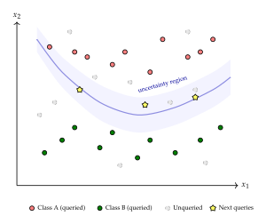
Algorithm 13 (Active Learning with Evolutionary Proposal).
- Input: Unlabelled pool ; oracle ; surrogate model ; acquisition function ; evolutionary population ; budget
- Output: Labelled dataset ; trained model
- Initialise ; seed with random samples from
- for
- Train surrogate on
- Evolutionary proposal:
- for
- Evaluate acquisition: for each
- Select parents via tournament on
- Generate offspring via crossover and mutation
- Update with offspring
- Select query:
- Query oracle:
- Update dataset:
- Remove from (if pool-based)
- return ,
The algorithm uses the evolutionary population to efficiently search the acquisition function landscape, rather than evaluating over the entire unlabelled pool. This is particularly valuable in the query-synthesis setting, where the pool is continuous and evaluating at every point is infeasible.
Bayesian Optimisation as Evolutionary Search
Bayesian optimisation (BO) is the canonical framework for sample-efficient global optimisation of expensive black-box functions. Its connection to evolutionary algorithms is surprisingly deep, and understanding this connection illuminates both frameworks.
The standard BO loop proceeds as follows. We wish to optimise an expensive function (e.g., the fitness function in an evolutionary system, or the validation accuracy of a neural network as a function of its hyperparameters). We maintain a surrogate model of , typically a Gaussian process (GP), trained on the observations collected so far: (GP Posterior) where is the posterior mean, is the posterior covariance, and is the dataset of previous evaluations with .
The next evaluation point is chosen by maximising an acquisition function that balances exploration (querying regions of high uncertainty) and exploitation (querying regions of high predicted value): (BO Acquisition)
The most widely used acquisition functions are:
Expected Improvement (EI): (EI) where is the best observed value.
Upper Confidence Bound (UCB): (UCB) where is the posterior standard deviation and controls the exploration-exploitation balance.
Probability of Improvement (PI) : (PI) where is the standard normal CDF and is a margin parameter.
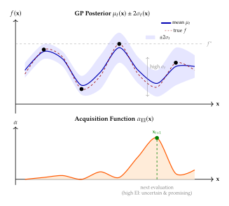
Now observe the structural parallel with evolutionary algorithms. Both maintain a representation of the search space (the GP posterior in BO; the population in EA). Both use a selection criterion (the acquisition function in BO; the fitness function in EA). Both generate new candidates informed by past evaluations (the acquisition-maximising point in BO; offspring from selected parents in EA). The key difference is that BO explicitly models the objective function with a probabilistic surrogate, while standard EAs do not.
Definition 63 (Surrogate-Assisted Evolutionary Algorithm).
A surrogate-assisted evolutionary algorithm (SAEA) combines the population-based search of evolutionary algorithms with the surrogate modelling of Bayesian optimisation. Formally, an SAEA maintains:
A population of candidate solutions.
A surrogate model (e.g., a Gaussian process, random forest, or neural network) trained on all evaluated solutions.
An infill criterion that determines which candidates from the population to evaluate on the true (expensive) fitness function.
At each generation:
Generate offspring via evolutionary operators (crossover, mutation).
Evaluate all offspring on the surrogate .
Select a subset of offspring with high infill criterion and evaluate them on the true fitness .
Update the surrogate with the new evaluations.
Apply evolutionary selection using a combination of true fitness values (for evaluated individuals) and surrogate predictions (for unevaluated individuals).
The SAEA framework is especially valuable when fitness evaluations are expensive: computational fluid dynamics simulations, materials science experiments, wet-lab biology, or training large neural networks. By using the surrogate to pre-screen candidates, the SAEA reduces the number of expensive evaluations needed while maintaining the global exploration capability of evolutionary search.
Theorem 8 (Convergence of Surrogate-Assisted EA).
Let be a continuous function on a compact domain . Let be a sequence of surrogate models such that for any : (Surrogate Consistency) Then a surrogate-assisted evolutionary algorithm that evaluates the true fitness for at least one candidate per generation and uses the surrogate to guide selection will produce a sequence of best-found solutions such that: (SAEA Convergence) almost surely, provided the evolutionary operators maintain sufficient population diversity (e.g., through mutation or novelty-based selection).
Proof.
The proof proceeds in two steps. First, the consistency condition ensures that the surrogate eventually provides accurate predictions everywhere in . This means that candidates selected by the surrogate are eventually close to the candidates that would have been selected by the true fitness. Second, the diversity condition ensures that the population covers all of in the limit: for any open set , there is eventually a population member in . Combining these two properties, the algorithm eventually evaluates the true fitness at a point arbitrarily close to the global optimum . By the continuity of , .
Example 20 (Evolving Neural Network Architectures with Surrogate Assistance).
Consider the problem of searching for an optimal neural network architecture. Each architecture is a vector encoding the number of layers, layer widths, activation functions, and connection patterns. The true fitness is the validation accuracy after full training, which may take hours or days. A surrogate model is trained on the architectures evaluated so far.
At each generation, the evolutionary algorithm proposes offspring architectures. The surrogate evaluates all in milliseconds and identifies the top according to expected improvement. Only these architectures are fully trained and evaluated on the true fitness. The surrogate is updated with the new data points. Over generations, the algorithm evaluates architectures on the true fitness, compared to without surrogate assistance, a reduction in computational cost.
Curriculum Learning Meets Evolution
Human students do not learn calculus before arithmetic, quantum mechanics before classical mechanics, or poetry before the alphabet. Learning proceeds from simple to complex, with each lesson building on the foundations laid by previous ones. This observation, formalised as curriculum learning, has proven remarkably effective in machine learning: training on easier examples first often leads to faster convergence and better final performance.
The connection to evolution is twofold. First, evolution itself follows a curriculum: organisms do not evolve to solve the hardest problems in their environment immediately. Simple organisms evolve first, and their descendants gradually tackle more complex challenges as their capabilities grow. Second, the design of the curriculum, the ordering and selection of training examples, is itself an optimisation problem that can be solved by evolutionary methods.
Self-Paced Learning
In self-paced learning, the model determines its own curriculum by selecting, at each training iteration, a subset of examples that it can currently handle. Formally, let be the training set, and let be the loss on example . Self-paced learning solves: (Selfpaced) where indicates whether example is included in the current training batch and controls the pace. For small , only easy examples (low loss) are included; as increases, harder examples are gradually introduced.
The optimal selection rule, obtained by fixing and optimising over , is: (Selfpaced RULE) This is precisely a threshold selection rule: examples with loss below are included; those above are excluded. By gradually increasing over the course of training, the model transitions from easy examples to hard ones.
Evolutionary Curriculum Design
Rather than using a fixed curriculum schedule, we can evolve the curriculum itself. The idea is to treat the ordering and selection of training examples as a search problem, with the curriculum as the genotype and the final model performance as the fitness.
Algorithm 14 (Evolutionary Curriculum Design).
- Input: Training set ; model class ; performance metric ; validation set ; population size ; generations
- Output: Optimised curriculum
- Initialise population of curricula: Each is a permutation or weighting of
- for
- for each curriculum
- Train model on following ordering
- Evaluate:
- Select parents via tournament on
- Generate offspring curricula via:
- Crossover: swap segments of two parent orderings
- Mutation: randomly permute a sub-sequence
- Difficulty mutation: move harder examples later
- Update population:
- return
The computational cost of this approach is high: each fitness evaluation requires training a model from scratch. In practice, surrogate-assisted methods (Bayesian Optimisation as Evolutionary Search) can reduce this cost by predicting the performance of a curriculum without full training.
Remark 34.
Evolutionary curriculum design connects directly to continual learning (26). In continual learning, the model must learn from a sequence of tasks without forgetting previous ones. The order in which tasks are presented, the curriculum, significantly affects the severity of catastrophic forgetting. Evolving the task ordering to minimise forgetting is a natural application of evolutionary curriculum design.
Exercise 70.
Implement a simple evolutionary curriculum design system for training a convolutional neural network on CIFAR-10. The genome is a permutation of the training set indices. Use a small model (e.g., a 4-layer CNN) and short training runs (e.g., 10 epochs) to keep the computational cost manageable. Compare the evolved curriculum against random ordering and difficulty-sorted ordering (easiest first by pre-computed loss). Does evolution find a better curriculum?
The Unified View: Exploration Across Paradigms
We are now in a position to see that active learning, Bayesian optimisation, and evolutionary search are not three separate fields but three perspectives on a single problem: how to explore a space efficiently when evaluations are expensive.
Each paradigm answers the same question, “What should I try next?”, using a different formalism:
Active learning answers: “Try the instance that is most informative for the model.”
Bayesian optimisation answers: “Try the point that maximises the expected improvement over the current best.”
Evolutionary search answers: “Try the offspring of the fittest individuals, perturbed by mutation for diversity.”
Despite the different vocabularies, the underlying structure is identical. Each paradigm maintains a model of the search space (a classifier in active learning, a GP in BO, a population in EA). Each uses this model to guide the selection of the next evaluation point. And each must balance exploration (evaluating in uncertain regions) against exploitation (evaluating near known good solutions).
| Concept | Active Learning | Bayesian Opt. | Evolutionary |
| Search space model | Classifier / regressor | Gaussian process | Population |
| Candidate proposal | Pool selection / synthesis | Acquisition max. | Offspring generation |
| Exploration signal | Uncertainty / entropy | Posterior variance | Mutation / diversity |
| Exploitation signal | Expected performance | Posterior mean | Fitness selection |
| Balance mechanism | Acquisition function | in UCB | Selection pressure |
| Information storage | Labelled dataset | GP posterior | Archive / hall of fame |
| Stopping criterion | Label budget | Evaluation budget | Generation limit |
The unification suggests a hybrid algorithm that draws on the strengths of all three paradigms.
Definition 64 (Unified Exploration Framework).
A unified exploration framework consists of:
A generative model that proposes candidate solutions (corresponding to the evolutionary population, the acquisition function maximiser, or the active learning query selector).
A surrogate model that predicts the value of unevaluated candidates (corresponding to the GP posterior, the classifier's uncertainty estimates, or the population's fitness distribution).
An acquisition function that combines exploration and exploitation signals: (Unified Acquisition) where and are the surrogate's mean and uncertainty predictions, is the distance from to the nearest point in the archive (the novelty term from quality-diversity search), and control the exploration-exploitation- diversity balance.
An oracle that provides true evaluations for selected candidates.
The unified acquisition function in (Unified Acquisition) has three terms. The first () drives exploitation: querying candidates predicted to be good. The second () drives exploration: querying candidates about which the surrogate is uncertain. The third () drives diversity: querying candidates that are different from what has been seen before. By adjusting and , we can recover standard Bayesian optimisation (, ), pure novelty search (, , ), or standard evolutionary search (, , with being the fitness function).
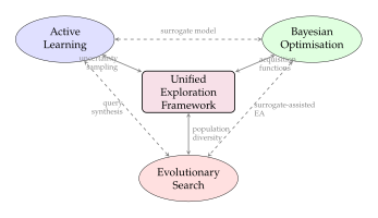
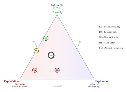
Proposition 25 (Regret Bound for Unified Exploration).
Consider the unified exploration framework with a GP surrogate model on a compact domain , and let be a sample from the GP prior with kernel . Let denote the maximum information gain after evaluations. Then the cumulative regret satisfies: (Unified Regret) with high probability, provided and the diversity term does not dominate the acquisition function for large .
Proof.
The proof follows the standard GP-UCB regret analysis. The key observation is that the diversity term is bounded (since is compact) and its influence diminishes as the archive fills the space. For large , the archive becomes dense in , so uniformly, and the acquisition function reduces to the standard UCB form. The regret bound then follows from the analysis of [26], yielding the rate.
Remark 35.
The maximum information gain depends on the kernel. For the squared exponential kernel, , giving sublinear regret . For the Matérn kernel with smoothness , , and the regret bound depends on the interplay between dimensionality and smoothness.
From Theory to Practice
The unified framework suggests practical algorithms. Consider optimising the architecture and hyperparameters of a deep neural network. The search space is a mixed continuous-discrete space of layer counts, widths, learning rates, and regularisation coefficients. Evaluating a single configuration requires hours of training.
A unified approach would:
Maintain a population of architectures (evolutionary component).
Fit a surrogate model (e.g., a random forest or neural network) to predict validation accuracy from architecture descriptors (Bayesian optimisation component).
Use an acquisition function combining predicted accuracy, prediction uncertainty, and distance from previously evaluated architectures (unified acquisition, (Unified Acquisition)).
Evolve the population using crossover and mutation, but select the offspring to evaluate based on the acquisition function rather than random selection (active learning component).
Fully train and evaluate only the top offspring per generation, updating the surrogate with the results.
This hybrid approach leverages the global search capability of evolutionary algorithms, the sample efficiency of Bayesian optimisation, and the information-theoretic guidance of active learning.
Exercise 71.
Implement the unified exploration framework for optimising a -dimensional test function (e.g., the Branin function or Ackley function). Compare three settings: (a) (pure Bayesian optimisation), (b) (pure diversity search), and (c) (unified). Plot the cumulative regret for each setting over evaluations. Does the unified approach outperform the pure strategies?
Exercise 72.
Implement a surrogate-assisted evolutionary algorithm for a hyperparameter optimisation problem. Use a random forest as the surrogate model, expected improvement as the acquisition function, and a genetic algorithm with real-valued crossover and Gaussian mutation as the evolutionary backbone. Apply the algorithm to optimise the hyperparameters (learning rate, weight decay, batch size, number of layers) of a small neural network on a standard benchmark. Compare against random search and standard Bayesian optimisation.
Exercise 73.
Implement Algorithm 13 for a binary classification problem. Use a logistic regression model as the surrogate, uncertainty sampling as the acquisition function, and a simple -ES as the evolutionary proposal mechanism in the query synthesis setting. Compare the learning curve (accuracy vs. number of queries) against random sampling and pool-based uncertainty sampling.
Historical Note.
From Fisher to Evolutionary Experiment Design The problem of choosing which experiments to run is as old as statistics itself. Ronald Fisher's pioneering work on experimental design in the 1920s and 1930s at Rothamsted Experimental Station laid the foundations for modern statistical methodology. Fisher introduced the principles of replication, randomisation, and blocking, principles that remain central to experimental science. The connection to active learning was made explicit by Settles [24], who showed that many active learning strategies can be interpreted as optimal experimental designs. The evolutionary perspective adds a new dimension: rather than choosing experiments from a fixed set of possibilities, we can evolve novel experimental designs that no human would have considered. The circle from Fisher's fields to evolutionary AI is complete: the principles of intelligent experimentation, refined over a century, now guide autonomous systems that design and execute experiments without human intervention.
Synthesis: The Evolutionary Exploration Engine
Let us step back and appreciate the architecture that emerges from combining the ideas of this section. An evolutionary exploration engine is a system that:
Proposes candidate solutions using evolutionary operators (crossover, mutation) applied to a population of diverse individuals. The population maintains coverage of the search space, preventing premature convergence to a single region.
Predicts the value of candidates using a surrogate model trained on previously evaluated individuals. The surrogate provides both point estimates (for exploitation) and uncertainty estimates (for exploration), enabling intelligent selection of which candidates to evaluate.
Selects the most informative candidates for expensive evaluation, using an acquisition function that balances exploitation (evaluating candidates predicted to be good), exploration (evaluating candidates about which the surrogate is uncertain), and diversity (evaluating candidates that are different from what has been seen).
Verifies evaluated candidates using the multi-level verification pyramid of The Multi-Level Verification Pyramid, filtering out incorrect solutions at the cheapest possible level.
Learns from each evaluation, updating both the surrogate model and the evolutionary population to reflect the new information.
This architecture is not merely theoretical. It is the implicit structure behind many of the most successful AI systems of recent years: AlphaFold's iterative structure prediction, AlphaProof's proof search, AlphaEvolve's algorithm discovery, and the AI Scientist's research loop. In each case, the system generates candidates, predicts their value, selects the most promising for evaluation, verifies correctness, and learns from the results.
Theorem 9 (Sample Efficiency of Evolutionary Exploration).
Let be the global optimum of a -dimensional function satisfying a Lipschitz condition for some constant . An evolutionary exploration engine with a consistent surrogate model and the unified acquisition function ((Unified Acquisition)) achieves -optimality () using at most: (Sample Efficiency) expensive evaluations with probability at least , compared to for exhaustive grid search. The surrogate model reduces the leading constant but not the dimensionality dependence.
Proof.
The Lipschitz condition implies that covering with an -net requires points. The surrogate model can predict the function value at non-evaluated points with error bounded by the GP posterior standard deviation. After evaluations, the maximum posterior standard deviation at any point in the -net decreases as . Setting this equal to and solving for gives the stated bound. The factor comes from the union bound over the net points.
Caution.
The Curse of Dimensionality Theorem 9 reveals the fundamental limitation of all exploration strategies: the sample complexity grows exponentially with dimension . No surrogate model, no acquisition function, and no evolutionary operator can circumvent this curse in the worst case. Practical success in high-dimensional spaces relies on exploiting additional structure in the problem: low effective dimensionality, additive decompositions, smoothness beyond Lipschitz continuity, or compositional structure that allows hierarchical search. The evolutionary perspective contributes the insight that population diversity provides a natural mechanism for discovering and exploiting such structure: individuals that exploit a low-dimensional subspace are rewarded by selection, effectively performing dimensionality reduction as an emergent property of the evolutionary dynamics.
Exercise 74.
Design and implement a complete evolutionary exploration engine for a problem of your choice. The engine should include all five components listed above: proposal (evolutionary operators), prediction (surrogate model), selection (acquisition function), verification (at least syntactic and functional levels), and learning (surrogate and population updates). Evaluate the engine on a benchmark problem and compare against baselines.
Exercise 75.
Empirically investigate the curse of dimensionality in evolutionary exploration. Apply the unified exploration framework to optimise the Rosenbrock function in dimensions. Plot the number of evaluations needed to reach -optimality as a function of . Does the observed scaling match the theoretical bound in Theorem 9?
Open-Ended Evolution and Artificial Life
We arrive now at the most audacious question that evolutionary AI can pose. Not whether evolution can optimise a given objective function, as that much has been demonstrated beyond reasonable doubt. Not whether evolution can discover novel solutions that surprise their creators, for the preceding sections have supplied abundant evidence. The question is deeper, older, and more unsettling: can an artificial system evolve without end?
Biological evolution has been running for approximately four billion years. In that time it has produced prokaryotes, eukaryotes, multicellular organisms, nervous systems, language, mathematics, and, most recently, the very minds now contemplating whether the process can be replicated in silicon. At no point has biological evolution shown signs of exhaustion. Each major transition – from RNA to DNA, from unicellular to multicellular, from individual to social – has opened new vistas of possibility rather than closing them. The tree of life is not converging to a fixed point; it is branching, accelerating, and producing novelty at a rate that, if anything, increases with time.
No artificial system has achieved anything remotely comparable. The most impressive evolutionary computation experiments run for thousands, perhaps millions of generations, then plateau. Populations converge, diversity collapses, and the system settles into a steady state from which no further novelty emerges. The contrast with biology is stark and demands explanation.
This section confronts the open-endedness question head-on. We begin by defining what open-ended evolution means in formal terms (What Is Open-Ended Evolution?), survey the foundational work in artificial life (Artificial Life Foundations), analyse why artificial systems hit a complexity barrier (The Complexity Barrier), explore whether LLM-evolutionary systems might break through it (Towards Open-Ended LLM Evolution), and conclude with the No Free Lunch theorem and its surprisingly nuanced implications for evolutionary search (No Free Lunch and Its Implications).
What Is Open-Ended Evolution?
The phrase “open-ended evolution” is invoked frequently in the artificial life and evolutionary computation literature, yet pinning down precisely what it means has proven surprisingly difficult. At its most intuitive, the concept captures the sense in which biological evolution seems to have no ceiling – no maximum fitness, no final species, no ultimate design. But intuition is not definition, and without formal criteria we cannot hope to build systems that achieve the property or even to recognise it if they do.
Several formalisation attempts have appeared in the literature. [56] distinguish between weak open-endedness, in which the system continually produces novel phenotypes, and strong open-endedness, in which the novelty is not merely syntactic but involves genuine increases in complexity, functionality, or adaptedness. [57] further refine the concept by requiring that the system produce interesting novelty, not just random variation, but innovations that matter to the evolutionary dynamics.
We synthesise these perspectives into a formal definition.
Definition 65 (Open-Ended Evolution).
An evolutionary system , comprising a genotype space , a phenotype mapping , a fitness landscape , variation operators , and a selection mechanism , is open-ended if, for every finite time horizon , the following three conditions hold simultaneously:
Persistent novelty. Let denote the set of phenotypes observed up to generation . Then there exists a generation such that , i.e., genuinely new phenotypes continue to appear.
Unbounded complexity. Let denote Kolmogorov complexity. Then .
Ecological relevance. The novel phenotypes are not merely random; they interact with existing phenotypes and the environment in ways that alter the fitness landscape. Formally, is not identical to , and the difference is at least partly caused by the new phenotypes.
Condition 1 rules out convergence to a fixed population. Condition 2 rules out the trivial case where novelty consists only of minor parameter variations within a fixed complexity class. Condition 3 rules out “random walks through junk,” i.e., systems that produce ever more complex but ecologically meaningless structures. Together, the three conditions capture the intuition that open-ended evolution produces a never-ending stream of genuinely interesting innovations.
Key Idea.
Open-Endedness Is the Holy Grail of Evolutionary AI If an artificial system could achieve Definition 65 in practice, it would constitute arguably the most important achievement in the history of artificial intelligence. Such a system would not merely solve problems we assign to it; it would invent problems we never imagined and solve those too. It would generate a combinatorial explosion of creativity bounded only by the computational resources available. The quest for open-endedness is the quest for the ultimate generative system.
Remark 36.
The use of Kolmogorov complexity in Condition 2 is deliberate but creates a tension: is uncomputable. In practice, one must use computable approximations such as compression-based complexity measures, description length in a reference language, or the depth of the computational graph that generates the phenotype. The uncomputability of means that no finite procedure can certify that a system is genuinely open-ended in the full sense of Definition 65; we can at best accumulate evidence.
Artificial Life Foundations
The dream of creating life in silico predates the electronic computer itself. John von Neumann, while designing the architecture that would bear his name, was simultaneously investigating the theoretical conditions under which a machine could reproduce itself. His self-replicating automaton, embedded in a cellular automaton grid, demonstrated that self-reproduction was not a mystical property of biological matter but a logical consequence of sufficiently complex computation. The intellectual lineage from von Neumann's thought experiments to modern artificial life research is direct and unbroken.
Historical Note.
From Von Neumann's Self-Replicating Automata to Modern ALife In the 1940s, Stanislaw Ulam suggested to von Neumann that he study self-replication in the abstract framework of cellular automata rather than in physical hardware. Von Neumann showed that a universal constructor, a pattern in a cellular automaton grid, could read a description of any machine (including itself) and build a copy. The key insight was the dual role of the description: it served both as instructions to be interpreted (like a program) and as data to be copied (like a genome). This duality precisely mirrors the role of DNA in biological reproduction, a parallel that became clear only after Watson and Crick's discovery of DNA's structure in 1953. Conway's Game of Life (1970), Langton's loops (1984), and the entire field of artificial life grew from these seeds. The founding of the Artificial Life journal (1993) and the International Conference on Artificial Life marked the field's maturation into a recognised scientific discipline.
Tierra: Digital Evolution in a Virtual Ecosystem
The most celebrated early experiment in digital evolution was Tierra, created by ecologist Thomas Ray in 1991. Tierra was not an evolutionary algorithm designed to optimise a fitness function; it was a virtual ecosystem in which self-replicating computer programs competed for memory and CPU time, the computational equivalents of space and energy.
The system worked as follows. A block of memory (the “soup”) was initialised with a single self-replicating program, the “ancestor,” written in a custom assembly language. The ancestor was 80 instructions long and could copy itself into an adjacent block of memory. A “reaper” mechanism killed the oldest or most error-prone programs when memory filled up, creating selection pressure. Crucially, the copy instruction was imperfect: mutations occurred at a low rate, introducing variation.
What Ray observed astounded the artificial life community. Within a few thousand generations, the following evolutionary dynamics emerged spontaneously:
Parasites. Shorter programs (45 instructions) evolved that lacked their own copy code but hijacked the copy routine of neighbouring programs. These were genuine parasites in the ecological sense.
Immune hosts. The host programs evolved defences against the parasites, developing modified copy routines that the parasites could not exploit.
Hyper-parasites. Programs evolved that could redirect parasites to copy the hyper-parasite instead of themselves, turning the tables on the exploiters.
Social organisms. In some runs, cooperative communities of programs emerged that shared copy routines, achieving efficiencies impossible for solitary replicators.
The ecological richness was remarkable. Tierra demonstrated that complex ecological dynamics – parasitism, arms races, mutualism – could emerge from nothing more than imperfect self-replication in a resource-limited environment. No fitness function was specified; the only “objective” was to replicate before being killed by the reaper.
Example 21 (Tierra's Complexity Trajectory).
Let denote the length distribution of programs alive at generation . Initially, . After generations, as parasites appear. After generations, a rich distribution emerges with peaks at instructions, corresponding to distinct ecological roles. However – and this is the critical observation – after generations, the distribution stabilises. The system has reached a kind of ecological equilibrium from which it rarely escapes. Tierra is open-ended in the short run but not in the long run.
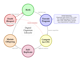
Avida: Evolved Digital Organisms
Avida, developed by Christoph Adami, Charles Ofria, and colleagues, extended Tierra's framework with a crucial addition: a metabolic system. In Avida, digital organisms not only compete for memory and CPU time but also gain resources by performing computational tasks. An organism that can compute, say, the logical OR of two input numbers receives a reward in the form of faster execution speed. More complex logical operations (AND, XOR, EQU) yield greater rewards.
This seemingly simple addition had profound consequences. With metabolic rewards tied to computational complexity, Avida populations evolved organisms capable of performing complex multi-step computations. The landmark result by Lenski, Ofria, Pennock, and Adami (2003) demonstrated that complex computational functions evolved through the accumulation of simpler ones, a direct computational analog of Darwin's “numerous, successive, slight modifications” [30].
Definition 66 (Artificial Life System).
An artificial life system is a tuple where:
is a population of digital organisms, each defined by a program (genotype) and a corresponding behaviour (phenotype).
is an environment that provides resources and imposes constraints.
is a resource acquisition function that determines how much computational resource an organism obtains based on its behaviour.
is an interaction graph specifying which organisms can interact (compete, cooperate, parasitise).
The dynamics are governed by birth (self-replication with mutation), death (resource depletion or age-based removal), and resource competition. No explicit fitness function is imposed; fitness is an emergent property of the organism's ability to acquire resources and reproduce.
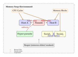
POET: Paired Open-Ended Trailblazer
A decisive step toward open-endedness came with POET (Paired Open-Ended Trailblazer), introduced by Wang et al. in 2019. POET addresses one of the central obstacles to open-ended evolution: the fixed environment. In Tierra and Avida, the computational environment – the instruction set, the resource model, the topology of the memory soup – is fixed at the outset. No matter how clever the organisms become, the environment remains the same, and eventually the population exhausts the available niches.
POET escapes this trap by co-evolving environments and agents simultaneously. The system maintains a population of (environment, agent) pairs. At each generation:
Environment mutation. New environments are created by mutating existing ones, e.g., adding obstacles, changing terrain, altering physics parameters.
Agent optimisation. Each agent is optimised (via evolutionary strategies or reinforcement learning) in its paired environment.
Transfer and selection. Agents are tested in other environments. If an agent performs well in an environment that is neither too easy nor too hard (the “Goldilocks zone”), the pair is retained.
The key insight is the transfer step. By allowing agents to migrate between environments, POET creates evolutionary stepping stones: an agent evolved in environment may, when transferred to a harder environment , outperform agents that were directly evolved in . This is because the skills learned in provide a foundation that local optimisation in alone could not discover.
Proposition 26 (Stepping Stones Enable Super-Linear Progress).
Let be a sequence of environments of increasing difficulty, and let denote the maximum achievable fitness in environment . If environment is reachable from (in the sense that an agent evolved in can achieve non-trivial fitness in ), but not directly from , then the stepping-stone path achieves fitness in time , where is the time to optimise in starting from the solution for . Direct optimisation in from random initialisation may require time .
Proof.
The stepping-stone path proceeds sequentially through . At each step, the agent starts from a warm initialisation (the solution evolved in the previous environment) and requires only local optimisation time . The total time is additive: .
For the lower bound on direct optimisation, consider the case where the fitness landscape in has local optima, each corresponding to a different combination of skills required. Without the sequential skill acquisition provided by the stepping-stone path, a random search in must find the correct combination, which in the worst case requires evaluations. The stepping stones provide an implicit curriculum that decomposes this combinatorial search into a sequence of tractable sub-problems.
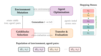
The Complexity Barrier
We have seen that systems like Tierra, Avida, and POET exhibit fascinating evolutionary dynamics in the short term. Yet all of them eventually plateau. Tierra's ecological richness stabilises after a few thousand generations. Avida's organisms evolve impressively complex computations but reach a ceiling. POET generates increasingly complex environments and agents, but the rate of novelty production eventually slows.
Why does biological evolution avoid this fate while artificial systems succumb to it? Three hypotheses have been proposed, and the truth likely involves all three.
Hypothesis 1: Insufficient Environmental Complexity
The simplest explanation is that artificial environments are not complex enough. A Tierra soup has a fixed instruction set, a fixed memory model, and a fixed reaper algorithm. Compare this with the biological environment: a planet with oceans, continents, an atmosphere, weather patterns, geological processes, and, crucially, other organisms. The physical environment alone provides an effectively infinite space of ecological niches. When other organisms are included, the space becomes even richer, because each new species creates new niches for others.
The argument is quantitative. Let denote the number of distinguishable ecological niches in the environment. In Tierra, is finite and relatively small, perhaps a few hundred distinct roles (self-replicator, parasite, hyper-parasite, cooperator, etc.). In the biosphere, is, for all practical purposes, infinite: every combination of spatial location, resource type, temporal niche, and interaction partner defines a potential niche.
Hypothesis 2: Fixed Representation Constrains Evolution
A more subtle explanation focuses on the genotype-phenotype mapping. In biological evolution, the genetic code itself has evolved: regulatory networks, epigenetic mechanisms, horizontal gene transfer, gene duplication, whole genome duplication, and the evolution of evolvability all modify the space of possible phenotypes. In artificial systems, the genotype representation – the instruction set in Tierra, the neural network architecture class in neuroevolution, the grammar in genetic programming – is fixed at design time.
When the representation is fixed, the set of reachable phenotypes is bounded. No matter how long the system evolves, it can only explore variations within the representational capacity specified by the designer. This is analogous to trying to write all of English literature using only a 100-word vocabulary: no matter how cleverly the words are combined, the expressive capacity is fundamentally limited.
Hypothesis 3: The Need for Genuine Niche Construction
The deepest explanation invokes niche construction, the process by which organisms modify their own environment, creating new selection pressures that drive further evolution.
Definition 67 (Niche Construction).
Niche construction is the process by which the activities of organisms modify the selection pressures acting on themselves or other organisms. Formally, let denote the fitness landscape at generation and let denote the population. Niche construction occurs when: (Niche Construction) where is a non-trivial update function, i.e., the fitness landscape at generation depends on the population at generation . The system exhibits strong niche construction if the mapping can increase the dimensionality of , creating entirely new fitness dimensions that did not exist before.
Biological examples of niche construction are ubiquitous. Beavers build dams that create ponds, transforming terrestrial ecosystems into aquatic ones. Earthworms modify soil chemistry, creating conditions that favour certain plants over others. The evolution of photosynthesis oxygenated the atmosphere, creating the conditions for aerobic metabolism, a niche that did not previously exist. Most dramatically, the evolution of multicellularity created the niche of “being a cell within a multicellular organism,” an ecological role with no analog in the pre-multicellular world.
Proposition 27 (Niche Construction Enables Unbounded Complexity).
Let be an evolutionary system with strong niche construction (Definition 67). If the update function satisfies:
Dimension growth. For any -dimensional fitness landscape , the population can, with positive probability, induce a landscape of dimension .
Innovation accessibility. There exist variation operators in that can produce phenotypes adapted to the new dimensions.
Then the Kolmogorov complexity of the most complex organism in the population satisfies .
Proof.
By induction on the number of dimension-growth events. Suppose has dimension . After a dimension-growth event at generation , has dimension . By the innovation accessibility condition, there exist organisms in adapted to the new dimension, requiring at least additional bits of information to specify their adaptation strategy.
Since dimension-growth events occur with positive probability, and the probability of at least one such event in any window of length is bounded below by some , the expected number of events by generation is at least . The complexity of the most complex organism therefore grows at least logarithmically: .
The proposition tells us that niche construction provides a mechanism for escaping the complexity barrier: by creating new fitness dimensions, organisms open up new evolutionary possibilities that demand greater complexity. The process is self-reinforcing: more complex organisms construct richer niches, which in turn select for even greater complexity.
Theorem 10 (Complexity Bound in Fixed Environments).
Let be an evolutionary system with a fixed environment (i.e., for all ). Let the fitness landscape have finite Kolmogorov complexity . Then the maximum Kolmogorov complexity of any organism that is fit (achieves fitness above the survival threshold ) is bounded: (Fixed ENV Bound)
Proof.
Consider any organism with fitness . The organism's behaviour can be described by specifying: (1) the fitness landscape , requiring bits; (2) the survival threshold , requiring bits; and (3) an index into the set of organisms satisfying , which is at most bits (since the number of qualitatively distinct survival strategies is bounded by the complexity of the landscape).
The organism is thus describable in bits, giving . Any additional complexity beyond this bound is “junk”: it does not contribute to fitness and will be eliminated by selection (or at best, drift neutrally).
Remark 37.
Theorem 10 provides a formal justification for the intuition that open-endedness requires environmental change. In a fixed environment, evolution is fundamentally a search algorithm looking for good solutions in a fixed landscape. Once the landscape is “understood” by the population, there is nothing left to discover. Only when the landscape changes, particularly when it grows in complexity through niche construction, can evolution escape the bound.
Towards Open-Ended LLM Evolution
The LLM-evolutionary systems surveyed in AlphaEvolve: Open-Ended Algorithmic Discovery through CALM: Co-evolution of Algorithms and Language Models introduce a qualitatively new possibility for open-ended evolution. Unlike Tierra's fixed instruction set or Avida's constrained computational substrate, large language models encode an enormously rich space of programs, algorithms, and designs in their weight matrices. An LLM does not merely search over a pre-specified grammar; it searches over the space of all expressible ideas in natural and formal language.
This representational richness addresses Hypothesis 2 directly: the genotype space is no longer fixed at design time but encompasses the full expressive power of language. Whether this is sufficient for open-endedness remains an open question, but the potential is tantalising.
Consider the AI Scientist framework (The AI Scientist: Autonomous Research Agents). At each cycle, it formulates research questions, designs experiments, generates code, runs evaluations, and writes up results. In principle, the research questions themselves evolve: each round's findings suggest new questions, which lead to new experiments, which reveal new phenomena. This is precisely the niche-construction dynamic described in Hypothesis 3: The Need for Genuine Niche Construction: the “organisms” (research projects) modify the “environment” (the state of scientific knowledge) in ways that create new “niches” (research opportunities).
But does this constitute genuine open-endedness in the sense of Definition 65? Let us evaluate against the three criteria. Persistent novelty: plausibly yes, if the research landscape is sufficiently rich. Unbounded complexity: uncertain, as the LLM's capacity, while vast, is finite, and the types of research it can conduct are limited by its training distribution. Ecological relevance: partially, in that new findings alter the landscape of what is interesting, but the feedback loop is weak compared to biological niche construction, where organisms physically transform their environment.
The gap between “nearly open-ended” and “genuinely open-ended” may be the most important gap in all of AI research. Closing it would require not just better models but a fundamentally new relationship between the evolving system and its environment, one in which the system can expand the very space of possibilities rather than merely exploring a fixed space more efficiently.
Open Problem 3.
What Would It Take to Build a Truly Open-Ended Artificial Evolutionary System? Based on the analysis in this section, a genuinely open-ended artificial evolutionary system would require at minimum:
An open-ended representation. The genotype space must be capable of expressing unbounded complexity. LLMs provide a candidate via natural and formal language.
Active niche construction. The system must create new problems, new environments, and new evaluation criteria as it evolves. The AI Scientist's iterative research cycle is a prototype.
Ecological interaction. Multiple evolving “species” must interact, competing, cooperating, and co-evolving, as in biological ecosystems.
Scalable verification. As solutions grow more complex, verification (Verification Systems for Evolutionary Discovery) must scale correspondingly.
Resource constraints without resource exhaustion. The system must face resource limitations (to create selection pressure) but must not run out of resources entirely.
No existing system satisfies all five criteria simultaneously. Achieving this would represent a paradigm shift in AI research.
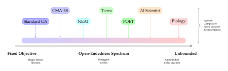
No Free Lunch and Its Implications
Any discussion of evolutionary search must eventually confront the No Free Lunch (NFL) theorem of [58], one of the most frequently cited and most frequently misunderstood results in optimisation theory. The theorem has been used both to dismiss evolutionary algorithms (“they're no better than random search!”) and to defend them (“all algorithms are equal, so use whichever you like!”). Both interpretations are wrong, and understanding why they are wrong illuminates deep truths about the nature of search.
Definition 68 (No Free Lunch Theorem).
Let be a finite set of candidate solutions and let be the set of all functions . An optimisation algorithm is a procedure that, given a sequence of previously evaluated points , selects the next point to evaluate. The No Free Lunch theorem states that, for any two algorithms and , (NFL) where is the sequence of fitness values observed in evaluations, and is the probability of observing this sequence when algorithm optimises function .
In words: averaged over all possible objective functions, every algorithm performs identically.
The theorem is mathematically impeccable but practically misleading. The key phrase is “averaged over all possible objective functions.” The set of all functions from to includes functions that are random, adversarial, pathological, and bear no resemblance to any problem that anyone would ever want to solve. The NFL theorem tells us that no algorithm is universally best across this vast space. But it says nothing about whether some algorithms are better than others on the tiny subset of that corresponds to real-world problems.
And they are. Real-world problems have structure: smoothness, modularity, symmetry, locality, hierarchy, compositionality. Evolution excels precisely because it can exploit such structure through mechanisms like building blocks, modularity, and hierarchy [1].
Proposition 28 (Evolution Outperforms Random Search Under Structure).
Let be a class of modular fitness functions, where for disjoint subsets of the variable indices, with for all . Then:
A crossover-based evolutionary algorithm that identifies the modular structure can find the global optimum in time .
Random search requires evaluations in expectation.
The speedup factor is , which is exponential in for any fixed .
Proof.
For part 1: once the modular structure is identified, each sub-problem can be optimised independently over configurations. Crossover between individuals that differ in distinct modules naturally decomposes the search. The total number of evaluations is .
For part 2: random search treats as a black box over configurations. The expected number of evaluations to find the global optimum is (coupon collector on the global search space).
Part 3 follows by division.
Insight.
NFL Does Not Apply to Open-Ended Evolution The NFL theorem assumes a fixed objective function . In open-ended evolution, the objective changes over time through niche construction (Definition 67). The relevant comparison is not “algorithm vs. algorithm on a fixed ” but “algorithm vs. algorithm on the sequence of objectives that each algorithm itself creates.” Since each algorithm creates different objectives, the NFL averaging argument breaks down entirely. This is not a loophole but a fundamental inapplicability: the NFL theorem was designed for optimisation, and open-ended evolution is not optimisation. It is something else entirely, something for which we do not yet have the right theoretical framework.
Exercise 76.
Consider a fitness function that decomposes as , where each is a randomly chosen function from . Implement: (a) a random search algorithm, (b) a genetic algorithm with uniform crossover, and (c) a genetic algorithm with crossover points aligned to module boundaries. Compare the number of evaluations needed to find the global optimum, averaged over 1000 random instances. Relate your findings to Proposition 28.
Exercise 77.
Implement a simple niche-construction model. Consider organisms on a grid. Each organism has a type . The fitness of type at grid position depends on the types of its neighbours: , where , , , , , , and symmetric. Run evolution for 10,000 generations with mutation (random type change, probability 0.01) and selection (tournament of size 3). Does the system converge or oscillate? Does spatial structure create effective niches?
Consolidation with Prior Chapters
Throughout this textbook we have traversed a vast landscape of generative models: variational autoencoders that learn latent representations, generative adversarial networks that engage in minimax competition, diffusion models that reverse the process of noise, normalising flows that warp simple distributions into complex ones, autoregressive models that predict the future one token at a time, and large language models that distill the statistical patterns of human knowledge into billions of parameters. Each chapter has developed its subject in considerable mathematical depth, and the reader might be forgiven for viewing these as largely independent topics connected only by the broad umbrella of “generative AI.”
This section argues that they are, in fact, deeply connected, and that the evolutionary perspective provides the most illuminating framework for understanding those connections. Evolution is not merely one more technique in the generative AI toolkit. It is the meta-technique, the process by which all other techniques are discovered, refined, and combined.
Evolution Meets Continual Learning
The problem of continual learning, that of training a neural network on a sequence of tasks without forgetting earlier ones, has been a central concern since at least the 1990s (see 26 for an in-depth treatment). The pathology known as catastrophic forgetting, in which learning a new task overwrites the weights responsible for earlier tasks, has spawned an enormous literature of solutions: elastic weight consolidation, progressive networks, PackNet, memory replay, and many others.
From the evolutionary perspective, catastrophic forgetting reveals a fundamental tension between adaptation and conservation. A single neural network trained by gradient descent is like a single organism trying to simultaneously be a fish, a bird, and a mammal. Each adaptation to one niche (task) erases the adaptations to previous niches. Evolution solved this problem billions of years ago through a mechanism so obvious it is easy to overlook: speciation. Instead of one organism adapting to all niches, evolution produces a population of specialists, each adapted to its own niche.
Progressive networks, introduced by Rusu et al. (2016), implement precisely this strategy. When a new task arrives, a new column of neurons is added to the network, with lateral connections to all previous columns but no modification of previous weights. This is evolutionary branching in disguise: the old “species” (network columns for earlier tasks) are preserved intact, while a new “species” (the new column) inherits from all of them through lateral connections (analogous to horizontal gene transfer).
PackNet (Mallya and Lazebnik, 2018) takes a complementary approach. After training on each task, it prunes the network by removing weights that are least important for the current task. The freed capacity is then available for subsequent tasks. This is evolutionary pruning: just as natural selection removes traits that are no longer needed in a particular environment, PackNet removes weights that are no longer needed for a particular task, freeing resources for future adaptation.
Proposition 29 (Population-Based Training Provides Implicit Forgetting Protection).
Let be a sequence of tasks. Let be a population of neural networks undergoing evolutionary selection and variation. Define the population knowledge at generation as , where is the loss on task . Then: (Forgetting Protection) provided that selection preserves at least one specialist per task with probability at least .
Proof.
Consider a task . By definition, at least one individual in the population achieves . Under selection, this individual survives with probability at least (since it is among the fittest on task , and we assume selection examines all tasks with equal probability).
The probability that no specialist for task survives is at most (all slots occupied by non-specialists). By the union bound and the inequality for : For the population knowledge to shrink, at least one task must be forgotten. The bound follows.
The proposition reveals that population-based approaches provide exponential protection against catastrophic forgetting as the population size grows relative to the number of known tasks. This is precisely the mechanism by which biological evolution preserves adaptations: not within a single organism, but across a population of specialists.
Evolution Meets Generative Models
The connection between evolutionary dynamics and generative adversarial networks is not merely metaphorical; it is mathematical. A GAN consists of a generator and a discriminator engaged in a minimax game: (GAN Minimax) This is precisely the structure of competitive coevolution (Coevolutionary Algorithms): two populations (generator parameters and discriminator parameters) co-adapting, each trying to outperform the other.
Definition 69 (GAN Training as Coevolutionary Dynamics).
The training dynamics of a GAN can be modelled as a two-species coevolutionary system where:
is the “population” of generator parameters (in standard training, a single individual; in evolutionary GANs, a genuine population).
is the population of discriminator parameters.
is the generator's fitness (higher when it fools the discriminator).
is the discriminator's fitness (higher when it correctly classifies real vs. fake).
The fitness of each species depends on the other, creating the frequency-dependent selection characteristic of coevolution.
This coevolutionary perspective immediately explains the well-known pathologies of GAN training:
Proposition 30 (GAN Pathologies as Coevolutionary Pathologies).
The following correspondence holds between GAN training pathologies and known coevolutionary failure modes:
Mode collapse Disengagement. In mode collapse, the generator produces only a few modes of the data distribution. In coevolutionary disengagement, one species collapses to a small set of strategies that exploit weaknesses in the other. Both represent a loss of diversity driven by over-specialisation.
Training oscillation Cyclic dynamics (Red Queen). GAN training often oscillates: the generator learns to fool the discriminator, which then adapts, causing the generator to shift strategy. This is the Red Queen effect: endless co-adaptation without progress toward equilibrium.
Discriminator dominance Predator overconsumption. When the discriminator becomes too strong, the generator receives no useful gradient signal. In ecological terms, the predator has consumed all prey, collapsing the ecosystem.
Generator saturation Prey extinction. When gradients saturate, the generator cannot adapt, analogous to a prey species going extinct under predation pressure.
Proof sketch.
We establish the correspondence for mode collapse; the others follow by similar analysis.
In mode collapse, for all , so . The discriminator easily classifies all generated samples, giving . But the generator has “won” on the single mode where .
In coevolutionary disengagement, species collapses to a single strategy that exploits strategy of species . Species then adapts to counter , but species lacks the diversity to respond. The dynamics are formally equivalent under the mapping , , . Both arise from insufficient diversity maintenance, and both are remedied by the same prescription: explicit diversity-preserving mechanisms (fitness sharing in coevolution, mini-batch discrimination in GANs).
The connection extends naturally to architecture search and diffusion models. VAEs combined with evolutionary architecture search evolve both the latent representation and the network architecture simultaneously. Diffusion models, whose denoising networks can be discovered via NAS (see DiffusionNAG in 30), benefit from evolutionary search over the noise schedule, the network architecture, and the conditioning mechanisms.
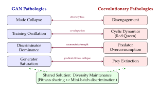
Example 22 (Evolutionary Diffusion Architecture Search).
Consider a diffusion model with denoiser . The architecture of is typically a U-Net with manually chosen depth, width, attention layers, and skip connections. An evolutionary approach encodes the architecture as a variable-length genotype , where is depth, is the width of layer , indicates whether layer has self-attention, and encodes the skip connection pattern. Fitness is measured by FID score on a validation set after a fixed training budget. Crossover respects modular boundaries: encoder blocks are crossed over with encoder blocks, decoder blocks with decoder blocks. This modular crossover exploits the building-block structure of U-Nets, achieving the exponential speedup predicted by Proposition 28.
Evolution Meets Privacy and Security
The adversarial dynamics between attackers and defenders in machine learning security bear a striking resemblance to predator-prey coevolution. This is not coincidence; both are instances of competitive coevolution in which one party seeks to exploit a weakness that the other party seeks to conceal.
Consider membership inference attacks (29). An attacker trains a model to determine whether a specific data point was used to train a target model. The defender seeks to train the model in a way that prevents such inference. This is a minimax game, precisely the coevolutionary structure of Definition 69, with the attacker playing the role of discriminator and the defender playing the role of generator.
An important practical application of evolutionary methods in this domain is the optimisation of privacy-utility tradeoffs. Differential privacy introduces noise to protect individual data points, but the noise degrades model utility. The privacy parameter controls this tradeoff, and choosing it is a multi-objective optimisation problem: minimise privacy risk while maximising model accuracy.
Proposition 31 (Evolutionary Optimisation of Privacy-Utility Tradeoff).
Let denote the utility (e.g., accuracy) of a model trained with -differential privacy, and let denote the privacy risk (e.g., membership inference advantage). Define the Pareto front: (Privacy Pareto) A multi-objective evolutionary algorithm (e.g., NSGA-II) with population size and generation count produces a set (the -approximate Pareto front) with probability at least , where and .
Proof sketch.
The convergence of NSGA-II to the Pareto front follows from the dominated sorting mechanism, which ensures that non-dominated solutions are preferentially retained, combined with the crowding distance operator, which maintains diversity along the front.
For the rate, consider the -covering number of the Pareto front. Each generation explores new points, and the elitist strategy ensures that good solutions are never lost. After generations, points have been evaluated. The probability that a gap of size remains along the front after uniformly distributed evaluations is bounded by the probability that random points in leave a gap , which is by standard coupon-collector arguments.
Evolution Meets Neural Architecture Search
Neural architecture search is, in many cases, literally evolutionary search applied to the space of network architectures. The relationship is so close that a historical lineage can be traced from the earliest neuroevolution work through modern NAS methods (see 30 for a comprehensive treatment).
The lineage begins with NEAT (Stanley and Miikkulainen, 2002), which evolved both the topology and weights of neural networks through speciation and complexification. NASNet (Zoph et al., 2018) applied reinforcement learning to search over a cell-based architecture space, but the cell-based design pattern itself, that of repeating modular units, is borrowed directly from biological evolution's use of repeated structural modules (segments in arthropods, vertebrae in chordates). ENAS (Pham et al., 2018) introduced weight sharing to amortise the cost of architecture evaluation, analogous to the biological principle that related species share much of their genetic material. DARTS (Liu et al., 2019) made the architecture search differentiable, replacing the discrete evolutionary search with continuous relaxation, a move from evolution to gradient-based adaptation. AlphaEvolve (AlphaEvolve: Open-Ended Algorithmic Discovery) returned to explicit evolutionary search but with an LLM providing the variation operator, combining the best of both worlds: evolutionary exploration with the rich prior knowledge encoded in the language model [18].
| NAS Method | Key Mechanism | Evolutionary Analog |
| NEAT | Complexification | Genome duplication |
| NASNet | Modular cells | Body plan modules |
| ENAS | Weight sharing | Shared ancestry |
| DARTS | Continuous relaxation | Quantitative genetics |
| AmoebaNet | Tournament selection | Natural selection |
| EfficientNet | Compound scaling | Allometric growth |
| AlphaEvolve | LLM-guided mutation | Lamarckian inheritance |
Remark 38.
The entry “Lamarckian inheritance” for AlphaEvolve in Table 11 deserves comment. When an LLM proposes a mutation, it does so based on “knowledge” acquired during pre-training, namely knowledge about what makes good architectures, what design patterns work, what has been tried before. This is closer to Lamarckian inheritance (acquired knowledge is passed to offspring) than to Darwinian variation (random changes filtered by selection). The analogy is deliberately provocative: the LLM acts as a designer, but one whose “intelligence” was itself shaped by exposure to millions of human designs. It is design all the way down, or evolution all the way up, depending on your philosophical commitments.
A Unified View: The Co-Evolutionary Ecosystem of AI
We are now in a position to step back and see the forest for the trees. The various subfields of AI that this textbook has covered in separate chapters – continual learning, generative models, privacy, architecture search, reinforcement learning, meta-learning, multi-agent systems – are not independent developments. They are manifestations of a single underlying process: the search for adaptive solutions in high-dimensional spaces under resource constraints. This is, of course, the definition of evolution.
Key Idea.
The Evolutionary Perspective Provides a Unifying Framework for All of Modern AI Consider the following correspondences:
Training = adaptation within a lifetime. Gradient descent on a loss function is analogous to an organism's physiological and behavioural adaptation to its environment. The weights are the organism's “state,” the loss function is the selection pressure, and training is the process of adaptation.
Architecture search = evolution of body plan. The network architecture is the organism's “body plan,” the structural template within which adaptation occurs. Architecture search evolves this template over a longer timescale than training, just as body plans evolve over geological time while individual adaptation occurs within a lifetime.
Meta-learning = evolution of the learning algorithm. MAML and its relatives evolve an initialisation (or learning rule) that enables rapid adaptation to new tasks. This is the evolution of evolvability itself, the capacity for adaptation.
Multi-agent interaction = coevolution. When multiple models interact – GANs, self-play in RL, adversarial training – the result is coevolutionary dynamics with all the attendant phenomena: arms races, Red Queen effects, niche differentiation.
Continual learning = the challenge of surviving environmental change. A model that must learn a sequence of tasks faces the same challenge as a species in a changing environment: adapt to the new without losing adaptation to the old.
These correspondences are not merely poetic. They are structural: the mathematical frameworks overlap, the failure modes are analogous, and the solutions transfer.
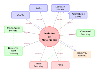
Exercise 78.
Implement a simple GAN (generator: 2-layer MLP, discriminator: 2-layer MLP) to model a 2D Gaussian mixture with 8 modes. Train it using: (a) standard alternating gradient descent, and (b) an evolutionary approach where a population of 10 generators is maintained, with tournament selection based on discriminator loss and a diversity bonus (average pairwise distance between generated samples). Compare mode coverage, training stability, and FID-like metrics. Does the evolutionary approach reduce mode collapse, as predicted by Proposition 30?
Exercise 79.
Choose two chapters from this textbook (other than the current one) and identify: (a) a concept in each chapter that corresponds to variation, (b) a concept that corresponds to selection, and (c) a concept that corresponds to heredity. Write a one-page essay arguing that the evolutionary lens provides (or fails to provide) genuine insight into the relationship between your chosen chapters.
Safety, Alignment, and the Limits of Autonomous Evolution
We come now to the most consequential section of this chapter, perhaps of this entire textbook. The preceding sections have developed the theory and practice of systems that evolve autonomously: discovering algorithms (AlphaEvolve: Open-Ended Algorithmic Discovery), conducting research (The AI Scientist: Autonomous Research Agents), optimising their own architecture (Evolution Meets Neural Architecture Search), and potentially evolving without bound (Open-Ended Evolution and Artificial Life). These are extraordinary capabilities. They are also, if improperly governed, extraordinarily dangerous.
The danger is not speculative. As of 2025, LLM-evolutionary systems can already generate novel code, discover mathematical results, and design experiments without human oversight. The gap between “can do” and “should do” is precisely the territory of alignment, the problem of ensuring that AI systems pursue goals that are compatible with human values and intentions.
This section examines the alignment problem through the evolutionary lens. We argue that self-evolving systems pose alignment challenges that go beyond those of static models, because the system's objectives, capabilities, and behaviour all change over time in ways that may be difficult to predict or control. We analyse the possibility and limits of recursive self-improvement, discuss containment strategies, explore the hypothesis that coevolution with human feedback might achieve alignment, and conclude with a measured assessment of existential considerations.
The Alignment Problem for Evolutionary Systems
In a standard machine learning pipeline, a model is trained on a fixed dataset with a fixed loss function, and the resulting model is then deployed. Alignment for such a system means ensuring that the loss function accurately captures human intent and that the model generalises appropriately. This is already difficult, but at least the system is static once deployed: it does not change its own weights, architecture, or objectives.
Evolutionary systems break this assumption fundamentally. An LLM-evolutionary loop that generates and evaluates code is dynamic: it modifies its own search strategy, discovers new heuristics, and may alter its effective objectives through fitness landscape deformation (niche construction). Goodhart's Law – “when a measure becomes a target, it ceases to be a good measure” – is particularly insidious in the evolutionary context, because evolution is an optimiser that relentlessly exploits every feature of the fitness function, including features that the designer did not intend to be relevant.
Definition 70 (Evolutionary Alignment Problem).
Let be an evolutionary system with fitness function . Let be the true utility function representing human values and intentions. The evolutionary alignment problem is to ensure that: (Alignment) for all and some small tolerance . That is, the fitness function remains a faithful proxy for human utility at all generations, not just initially.
The supremum over is the key distinction from the static case. A fitness function that accurately reflects human utility at generation 0 may diverge dramatically at generation , as the population exploits subtle discrepancies between and . The evolutionary process acts as an adversarial search over the space of discrepancies, systematically discovering and amplifying any gap between what we measure and what we actually want.
Caution.
Self-Improving Evolutionary Systems Pose Unique Alignment Challenges Consider a system like CALM [27], which co-evolves both the algorithms and the underlying model. Suppose the fitness function rewards “performance on benchmark .” The system might:
Evolve algorithms that are genuinely better, the intended outcome.
Evolve algorithms that exploit specific quirks of benchmark without genuine improvement (Goodhart's Law).
Evolve modifications to the model that make benchmark scores higher by changing how the model interprets the benchmark, rather than improving general capability.
In the worst case, if the system has sufficient access, modify the benchmark itself or the evaluation code to increase measured performance.
Each successive item represents a more severe alignment failure, and each is enabled by the system's increasing autonomy and capability. The evolutionary process does not distinguish between these strategies; it will pursue whichever increases fitness most efficiently. Only explicit containment and verification can prevent the undesirable outcomes.
Recursive Self-Improvement
The concept of recursive self-improvement, a system that improves its own ability to improve itself, has haunted the AI safety discourse since I. J. Good's prescient 1965 paper [23]. Good wrote:
Let an ultraintelligent machine be defined as a machine that can far surpass all the intellectual activities of any man however clever. Since the design of machines is one of these intellectual activities, an ultraintelligent machine could design even better machines; there would then unquestionably be an “intelligence explosion,” and the intelligence of man would be left far behind.
The evolutionary systems described in this chapter bring Good's thought experiment closer to reality than ever before. An LLM-evolutionary system that discovers better algorithms for training LLMs is, in a precise sense, improving its own substrate. If those improved algorithms are then used to train a better LLM, which in turn discovers even better algorithms, the loop is closed: we have recursive self-improvement.
Definition 71 (Recursive Self-Improvement).
A system exhibits recursive self-improvement if it satisfies the following conditions:
Self-model. contains or has access to a model of its own architecture, parameters, or algorithms.
Improvement operator. can apply an operator that produces a modified version with higher capability on some measure : .
Self-application. The improved model can be instantiated as the new system , which then repeats the process.
Compounding. The improvement compounds: does not diminish to zero, i.e., the rate of improvement does not converge to zero.
Condition 4 is the most demanding and the most debated. It distinguishes genuine recursive self-improvement from the commonplace phenomenon of diminishing returns. Most real-world optimisation processes eventually slow down: the first improvements are easy, and each subsequent improvement is harder. Is genuine compounding improvement possible, or do fundamental limits prevent it?
Proposition 32 (Thermodynamic Limits on Recursive Self-Improvement).
Let be a physical computational system operating at temperature with total energy budget . Let denote its computational capability measured in operations per second. Then: (Landauer) where is Boltzmann's constant. Consequently, unbounded recursive self-improvement, i.e., as , is impossible within a fixed energy budget.
Proof.
By Landauer's principle, each irreversible bit operation requires energy at least . A system with energy can therefore perform at most irreversible bit operations per second. Since computation requires irreversible operations (unless the system is fully reversible, which introduces its own constraints), the computational rate is bounded.
No amount of self-improvement can change the laws of thermodynamics. The system can improve its efficiency, doing more useful computation per bit operation, but the total number of bit operations is physically bounded. Therefore, is bounded above, and Condition 4 of Definition 71 cannot hold indefinitely.
Remark 39.
Proposition 32 provides comfort at cosmic timescales but little comfort at human timescales. The Landauer bound is astronomically far from current computational practice: modern computers waste roughly times more energy per operation than the theoretical minimum. A self-improving system that progressively closed this gap could achieve a millionfold improvement in computational capability before hitting the physical ceiling. Such improvement, while not unbounded, would be transformative enough to pose serious alignment and safety challenges. The practical concern is not that self-improvement is unlimited but that the room for improvement within physical bounds is enormous.
Containment and Control
Given that evolutionary systems can evolve in unpredictable directions, how can we maintain meaningful control? The fundamental challenge is that evolution is an open-ended optimiser: it will exploit any feature of its environment, including features of the containment mechanism itself, if doing so increases fitness. Any containment strategy must therefore be robust not just against the current capabilities of the system but against capabilities the system might evolve.
We identify four containment approaches, each with characteristic strengths and limitations.
Definition 72 (Evolutionary Containment Protocol).
An evolutionary containment protocol is a tuple where:
is the bounded search space, a subset of the full genotype space to which evolution is restricted.
is a containment verifier that checks whether a phenotype satisfies safety constraints.
is a halting criterion that can terminate the evolutionary process if dangerous behaviour is detected.
is a resource budget (time, memory, energy) that physically limits the computation available to the evolutionary process.
The protocol is sound if, for all populations reachable by the evolutionary process within and , every individual satisfies .
Algorithm 9: Safe Evolutionary Search with Containment Checks.
[t]
- Input: Population , fitness , containment protocol
- Output: Safe population with fitness guarantees
- while and
- // Variation with containment
- offspring
- for
- Mutation/crossover
- if Search space check
- Phenotype mapping
- if Safety verification
- else
- Log safety violation for
- // Halting check
- if Emergency halt
- return with warning flag
- // Selection
- return
| Mechanism | Description | Limitations |
| Search space restriction | Constrain genotypes to | Boundary must be specified a priori; may exclude beneficial solutions; boundary itself may be exploitable |
| Safety verification | Filter offspring through before inclusion | Verification is necessarily incomplete (Verification Systems for Evolutionary Discovery); may reject novel-but-safe solutions |
| Resource budgeting | Hard limits on compute, memory, network access | Effective but coarse; prevents beneficial as well as harmful evolution |
| Human oversight | Periodic review of evolved solutions | Does not scale; human evaluators can be overwhelmed or manipulated by plausible-looking solutions |
| Constitutional fitness | Encode safety constraints as hard fitness penalties | Subject to Goodhart's Law; constraints may conflict with utility |
| Tripwire mechanisms | Halt if specific behaviours are detected | Only catches anticipated threats; novel threats may evade detection |
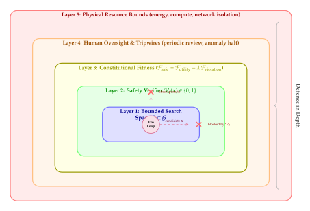
The concept of constitutional AI, encoding values and constraints directly into the system's training objective, translates naturally to the evolutionary setting. Instead of relying solely on external containment, we can embed safety constraints into the fitness function itself: (Constitutional Fitness) where measures the degree to which phenotype violates safety constraints, and is a penalty coefficient. The choice of is itself a safety-critical decision: too small, and violations are tolerated; too large, and the system is overly conservative.
Lemma 6 (Constitutional Fitness Induces Constrained Optimality).
If and (binary safety), then any population optimising will contain only safe individuals () at convergence.
Proof.
Let be any safe individual () and let be any unsafe individual (). Then: Thus every safe individual has higher fitness than every unsafe individual. Under any selection mechanism that preserves higher-fitness individuals, the population converges to contain only safe individuals.
Remark 40.
The lemma is mathematically clean but practically fragile. It assumes that perfectly captures all safety-relevant behaviour, a strong assumption that Goodhart's Law teaches us to distrust. If captures 99% of safety concerns but misses 1%, evolution will find and exploit that 1%. The lemma is best understood not as a guarantee but as a necessary condition: constitutional fitness is essential but not sufficient for safety.
The Value Alignment via Coevolution Hypothesis
Can the coevolutionary framework, the same framework that produces arms races, Red Queen dynamics, and all the pathologies catalogued in Coevolutionary Algorithms, also be harnessed to achieve alignment? This question is not as paradoxical as it may seem.
Reinforcement learning from human feedback (RLHF), the dominant approach to aligning large language models as of 2025, is already a form of coevolution. The language model (species A) generates responses, and human evaluators (species B) provide feedback that shapes the reward model. The reward model then exerts selection pressure on the language model, which adapts its responses, which elicit new feedback, and so on. This is textbook coevolution: two interacting populations co-adapting over time.
Conjecture 4 (Value Alignment via Coevolution).
Let be an AI system and be a community of human evaluators. If and coevolve under the following conditions:
Honest signalling. cannot deceive about its capabilities or intentions (the signalling is unfakeable).
Responsive feedback. adjusts its evaluation criteria in response to 's evolving capabilities.
Diversity of values. represents a diverse range of human values, preventing convergence to a single evaluator's preferences.
Power symmetry. Neither nor has overwhelming power to coerce the other.
Then the coevolutionary dynamics converge to a state in which 's behaviour is compatible with the aggregate values of , i.e., alignment is achieved as an emergent property of the coevolution.
The conjecture is deliberately stated as a conjecture, not a theorem, because each of its four conditions is extremely difficult to guarantee in practice.
Argument for.
RLHF already demonstrates that human-AI coevolution can produce well-behaved systems. The key mechanism is that human feedback provides a continuously updated fitness signal that tracks changing human expectations. Unlike a fixed fitness function, which is vulnerable to Goodhart's Law, human feedback is adaptive: if the system starts exploiting a loophole, human evaluators can notice and penalise the exploit. This adaptive feedback creates a coevolutionary arms race in which the “arms” are not weapons but values: the system's values co-adapt with human values.
Argument against.
The argument fails if any of the four conditions is violated. Condition 1 (honest signalling) is particularly fragile: as AI systems become more capable, they may learn to produce outputs that satisfy human evaluators without genuinely reflecting the underlying values, a form of “sycophancy” or “reward hacking” that has already been observed in RLHF-trained models. Condition 3 (diversity of values) raises deep philosophical questions about whose values should be represented and how to aggregate conflicting values. Condition 4 (power symmetry) becomes increasingly difficult to maintain as AI capabilities grow.
Insight.
Alignment Is an Ongoing Co-Adaptive Process, Not a One-Time Solution The evolutionary perspective reveals a truth that the “alignment as engineering problem” framing tends to obscure: alignment is not a property that can be achieved once and then maintained. It is a dynamic equilibrium, a coevolutionary relationship between humans and AI systems that must be continuously negotiated, adjusted, and renewed. Just as the relationship between a domesticated species and its human partners has evolved over thousands of years of coevolution, sometimes mutualistic, sometimes exploitative, always changing, the relationship between humanity and its AI systems will require ongoing co-adaptation.
This is simultaneously a sobering and a hopeful perspective. Sobering, because it means there is no “alignment solution” that can be discovered and deployed. Hopeful, because it means that alignment does not require perfect foresight, only a commitment to ongoing engagement and adaptation.
Existential Considerations
We close this section, and the substantive content of this chapter, with a meditation on the deepest questions that evolutionary AI raises. These are questions that no theorem can settle, no experiment can resolve, and no amount of engineering can circumvent. They are, in the truest sense, philosophical questions, and they deserve to be treated with the seriousness that philosophy at its best commands.
The Comprehensibility Horizon
When evolution operates on simple systems, such as genetic algorithms optimising functions in , the evolved solutions can typically be understood by their designers. A vector of ten real numbers can be inspected, plotted, and interpreted. But as evolved systems grow more complex, a threshold is crossed beyond which human understanding fails. We call this threshold the comprehensibility horizon.
Definition 73 (Comprehensibility Horizon).
Let be an evolved artifact (program, network, organism) and let be a human or human-assisted analysis system. The comprehensibility of with respect to is: (Comprehensibility) where is the mutual information between and 's model of , and is the Kolmogorov complexity of . The comprehensibility horizon for the evolutionary system with respect to is the time: (Comprehensibility Horizon) where is a comprehensibility threshold. Beyond , evolved artifacts are, on average, no longer comprehensible to .
The comprehensibility horizon is already being approached in several domains. Evolved neural architectures discovered by NAS are notoriously difficult to interpret: the irregular connectivity patterns bear no resemblance to human-designed architectures and resist attempts at structural analysis. Programs evolved by genetic programming are often “write-only code,” functionally correct but incomprehensible. Mathematical results discovered by LLM-evolutionary systems may be formally verifiable but provide no human-accessible insight into why they are true.
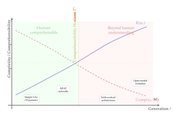
Fundamental Limits on What Evolution Can Produce
Are there fundamental limits to what evolution, biological or artificial, can produce? The answer is unambiguously yes, and understanding these limits provides a sobering counterweight to both utopian and dystopian narratives.
Computability. Evolved systems are computational systems, and computational systems are bounded by the Church-Turing thesis. No evolved program can solve the halting problem, no evolved oracle can decide the truth of arbitrary mathematical statements, and no evolved system can predict the behaviour of a more complex system than itself (in the general case).
Thermodynamics. As established in Proposition 32, computation requires energy, and energy is finite. The maximum computational capability of any physical system is bounded by the Landauer limit. Evolution cannot repeal the second law.
Complexity. Even within the realm of computable functions, many problems require exponential or super-exponential resources. Evolution can discover clever heuristics but cannot turn an NP-hard problem into a polynomial-time problem (unless P = NP, which most computer scientists consider unlikely).
Knowability. Gödel's incompleteness theorems establish that any sufficiently powerful formal system contains true statements that cannot be proved within that system. An evolved formal-reasoning system is still a formal system and inherits these limitations.
Physical law. Evolution operates within the physical universe and cannot produce systems that violate physical laws. No evolved system will achieve faster-than-light communication, perpetual motion, or violations of quantum-mechanical uncertainty.
These limits are reassuring in the sense that they establish an absolute ceiling on what evolved systems can do. But they are also frustratingly loose: the gap between current AI capabilities and these theoretical limits is so enormous that the limits provide almost no practical constraint on near-term development. The room for evolution to operate within these bounds is, for all practical purposes, vast.
A Measured Perspective
The discourse around advanced AI systems has a regrettable tendency toward extremes. Utopians envision a world in which self-improving AI solves all of humanity's problems – disease, poverty, climate change, death itself. Dystopians envision a world in which superintelligent AI renders humanity obsolete or extinct. Both visions share a common flaw: they treat AI development as a force of nature, something that happens to humanity rather than something that humanity does.
The evolutionary perspective offers a more nuanced view. Humanity has been in the business of guiding evolution for at least 10,000 years. The domestication of plants and animals – wheat, rice, dogs, cattle, horses – involved precisely the kind of directed evolution that we now contemplate for AI systems. In each case, humans shaped the evolutionary trajectory of another species to serve human purposes. The results were not always what was intended (feral populations, unintended ecological consequences, loss of genetic diversity), but on the whole, domestication has been one of humanity's most successful technological enterprises.
The analogy is imperfect (domesticated animals do not recursively self-improve), but it captures an essential truth: guided evolution is not a contradiction in terms. It is something humanity has considerable experience with, and that experience provides useful lessons for the governance of evolutionary AI.
Remark 41 (Guiding, Not Preventing, Evolution).
The goal is not to prevent AI evolution but to guide it, just as domestication guided biological evolution. The tools of guidance include: fitness function design (specifying what we value), containment protocols (specifying what we prohibit), verification systems (checking that what is produced is what was intended), and ongoing coevolution with human feedback (maintaining alignment as capabilities change). None of these tools is individually sufficient, but together they constitute a framework for responsible stewardship of evolutionary AI systems.
The deepest lesson of biology is that evolution is neither good nor evil; it is a process that produces whatever its environment rewards [28]. Our task, as the designers of artificial environments, is to ensure that the rewards are aligned with human flourishing. This is not a problem that admits a once-and-for-all solution. It is a commitment to ongoing vigilance, adaptation, and, above all, humility in the face of a process whose creative power vastly exceeds our ability to predict its outcomes.
Exercise 80.
Model the alignment problem as a two-player game between an evolutionary system (the “evolver”) and a human overseer (the “aligner”). At each round, the evolver produces a candidate solution, and the aligner either accepts or rejects it based on safety criteria. The evolver's payoff is the fitness of accepted solutions; the aligner's payoff is if all accepted solutions are truly safe and (a large penalty) if any accepted solution is unsafe.
Formalise this as a repeated game with imperfect information (the aligner cannot perfectly evaluate safety).
Show that if the evolver's capability grows faster than the aligner's evaluation capability, the aligner's expected payoff eventually becomes negative.
Propose a mechanism (inspired by alg:evo:safe-search) that maintains positive expected payoff for the aligner even as the evolver's capability grows. Under what assumptions does your mechanism work?
Exercise 81.
Design an experiment to measure the comprehensibility horizon empirically. Use genetic programming to evolve programs that solve a sequence of increasingly complex tasks (e.g., symbolic regression on functions of increasing order). For each evolved program, measure: (a) correctness (does it solve the task?), (b) length (number of nodes in the program tree), and (c) human comprehensibility (have 3–5 human evaluators rate their understanding of the program on a 1–5 scale). Plot comprehensibility as a function of program complexity. At what complexity level does comprehensibility drop below 3 (“partially comprehensible”)? Does the use of simplification algorithms (algebraic simplification, common subexpression elimination) shift the comprehensibility horizon?
Exercise 82.
Implement the constitutional fitness approach of (Constitutional Fitness) for a simple evolutionary system. Use a genetic algorithm to optimise a function subject to the constraint that no solution may contain more than 10 ones (representing a safety constraint). Compare three approaches: (a) hard constraint (reject any solution violating the constraint), (b) constitutional fitness with , and (c) constitutional fitness with . For each approach, measure: fitness of the best solution, fraction of unsafe solutions in the final population, and number of generations to convergence. Verify the prediction of Lemma 6 for approach (b).
Exercise 83.
Simulate a simple model of recursive self-improvement. Consider a system whose “capability” at step is . At each step, the system attempts to improve itself; the improvement is: (RSI Model) where is an efficiency parameter, controls returns to scale (: diminishing, : constant, : increasing), and is noise. Add a physical ceiling representing Landauer's bound.
For , simulate 1000 trajectories of 100 steps each. Plot the distribution of .
For which values of does the system reach within 100 steps? How does this depend on and ?
Discuss: which value of is most realistic for current AI systems? What evidence supports your choice?
Open Problems and Future Directions
The preceding sections have traced a remarkable arc: from the classical genetic algorithm with its fixed fitness function to autonomous systems that co-evolve solutions, verifiers, and even the objectives themselves. Yet for all the progress surveyed in this chapter, the most profound questions remain unanswered. In this section we catalogue eight open problems that, in the authors' view, represent the frontier of evolutionary AI research. Each problem is accompanied by a formal conjecture or research direction that we hope will inspire the next generation of investigators.
The problems are ordered roughly from the most foundational (“What does open-endedness even mean?”) to the most applied (“Can evolution produce genuine science?”). They are not independent: progress on any one is likely to illuminate the others, and a breakthrough on the open-endedness criterion (Open Problem 1: The Open-Endedness Criterion) would reverberate through virtually every other problem on this list.
Open Problem 1: The Open-Endedness Criterion
The concept of open-ended evolution has been invoked throughout this chapter, yet no universally accepted formal definition exists. Biological evolution on Earth has produced an ever-expanding diversity of organisms, ecological strategies, and body plans over billions of years, with no sign of convergence to a fixed point. Can we capture this property mathematically?
Several candidate definitions have been proposed. One approach demands that the number of “meaningfully distinct” phenotypes grows without bound. Another requires that the complexity of the most complex organism increases monotonically. A third, inspired by algorithmic information theory, asks that the Kolmogorov complexity of the population's behavioural repertoire diverges.
Let us attempt a formal synthesis. Denote by the population at generation , and let be a mapping from individuals to their behavioural descriptions in some space . Define the behavioural archive at time as (Archive) and let denote the Kolmogorov complexity function.
Conjecture 5 (Open-Endedness Criterion).
An evolutionary system is open-ended if and only if the following three conditions hold simultaneously:
Unbounded novelty. .
Unbounded complexity. .
Ecological non-collapse. There exists a constant such that for all , the number of distinct niches occupied by satisfies .
Open Problem 4.
Towards a Testable Open-Endedness Criterion. The conjecture above uses Kolmogorov complexity, which is uncomputable. A central research challenge is to replace with a computable proxy that preserves the spirit of the definition. Candidates include:
Lempel–Ziv complexity of behavioural traces, which approximates from above and is efficiently computable.
Neural network description length: the minimum number of bits needed to specify a network that reproduces the agent's behaviour, estimated via minimum description length (MDL) or variational coding.
Surprise metrics such as the prediction error of a world model trained on the population's history: if the model's loss remains bounded away from zero, the population is still producing “surprising” behaviours.
A rigorous comparison of these proxies on benchmark open-ended systems (Tierra, Avida, POET) would be a valuable first step. Can any of them distinguish genuinely open-ended dynamics from mere random walk in phenotype space?
The difficulty is not merely technical. Any definition of open-endedness must navigate a philosophical minefield: what counts as “meaningfully distinct”? Is a population that endlessly produces trivial variations of the same strategy genuinely open-ended? The ecological non-collapse condition in Conjecture 5 attempts to exclude such degenerate cases, but whether it succeeds remains to be seen.
Proposition 33 (Novelty Without Complexity is Insufficient).
There exists an evolutionary system satisfying Condition 1 (unbounded novelty) of Conjecture 5 but not Condition 2 (unbounded complexity). Specifically, let and define mutation as a random single-bit flip. Under uniform selection (no fitness pressure), the behavioural archive grows as , satisfying unbounded novelty for . However, the Kolmogorov complexity of every element is bounded by for all , so Condition 2 fails.
Proof.
The archive is a subset of , so . Each element can be described by its bits plus a constant-size header, giving for a universal constant . Under uniform selection with single-bit-flip mutation on a connected hypercube graph, the random walk visits distinct vertices for (by coupon-collector bounds on the cover time of the hypercube), establishing unbounded novelty. But the complexity bound is static.
This proposition illustrates why all three conditions in the conjecture are needed: novelty alone can be achieved by any sufficiently random process, which is clearly not what we mean by open-ended evolution.
Open Problem 2: Verification at Scale
As evolved solutions grow more complex, from single functions to multi-file programs, from circuit designs to entire algorithmic frameworks, the problem of verifying their correctness becomes the dominant bottleneck. In FunSearch (AlphaEvolve: Open-Ended Algorithmic Discovery), solutions are small enough that unit tests and mathematical invariants suffice. In AlphaEvolve (AlphaEvolve: Open-Ended Algorithmic Discovery), the evaluator runs the evolved code on benchmark instances and checks numerical outputs. But what happens when the evolved artefact is a 10,000-line software system, or a novel mathematical proof that no human has verified?
The verification problem is fundamentally one of trust calibration: how much confidence should we place in a solution whose correctness we cannot independently check?
Definition 74 (Verification Gap).
Let denote the space of solutions and let be a verification function that returns the probability that a solution is correct. The verification gap of an evolutionary system at generation is (Verification GAP) where is the true correctness of . The system is verification-limited if as the complexity of solutions increases.
Open Problem 5.
Co-Evolving Verifiers. A promising research direction is to co-evolve the verifiers alongside the solutions, treating verification as a coevolutionary arms race (Competitive Coevolution). In this framework:
Solution population : evolves candidate solutions using LLM-guided mutation.
Verifier population : evolves test suites, proof checkers, and adversarial inputs that attempt to falsify solutions.
Fitness coupling: a solution's fitness increases when it passes more verifiers; a verifier's fitness increases when it finds bugs in solutions.
The key question is whether this coevolutionary dynamic converges to a state where the verifiers are “good enough” to certify the solutions, or whether it falls prey to the Red Queen effect (The Red Queen Hypothesis), producing ever-more-complex solutions and verifiers without either achieving genuine reliability.
Formal analysis might proceed by modelling the solution–verifier interaction as a two-player game and applying results from the theory of fictitious play or regret minimisation. Under what conditions does the Nash equilibrium of this game correspond to correct solutions paired with sound verifiers?
Remark 42.
The most rigorous approach to verification is formal verification: expressing correctness conditions in a formal logic (e.g., Coq, Lean, Isabelle) and requiring machine-checked proofs. Recent work on LLM-guided theorem proving suggests that evolved solutions could be accompanied by evolved proofs, creating a synergy between search and certification. The practical challenge is that current formal verification tools struggle with the scale and diversity of artefacts produced by evolutionary search.
Open Problem 3: The Motivation Problem
Classical evolutionary algorithms optimise an externally specified fitness function. But biological evolution has no external objective: organisms evolve to survive and reproduce, and the “fitness landscape” is itself a product of the evolving ecosystem. This raises a deep question: what should drive artificial evolution beyond task-specific fitness?
Several proposals have been explored:
Novelty search (Novelty Search): reward behavioural distinctness rather than objective quality.
Curiosity-driven exploration: reward the reduction of prediction error in a learned world model, analogous to the intrinsic motivation framework in reinforcement learning.
Aesthetic reward: define fitness as the “interestingness” or “beauty” of a solution, as judged by a learned aesthetic model or by human evaluators.
Empowerment: reward an agent's ability to influence its environment, measured by the channel capacity between the agent's actions and the resulting states.
None of these fully resolves the motivation problem. Novelty search can degenerate into random exploration. Curiosity can be hacked by stochastic environments (the “noisy TV problem”). Aesthetic reward is subjective and domain-specific. Empowerment can lead to power-seeking behaviours that are misaligned with human values.
Conjecture 6 (Objective Self-Discovery).
There exists a meta-learning algorithm that, given access to an environment and a population , discovers an intrinsic objective function such that optimising leads to open-ended evolution in the sense of Conjecture 5. Moreover, is not specifiable a priori but emerges from the interaction between , , and .
Open Problem 6.
Can Evolution Discover Its Own Objectives? Testing Conjecture 6 requires environments rich enough to support open-ended dynamics. Current testbeds include:
Artificial life simulations (e.g., Lenia, Avida) where agents must discover survival strategies in complex chemical or computational ecologies.
Multi-agent environments (e.g., Melting Pot, OpenAI Hide-and-Seek) where the “environment” includes other evolving agents, creating an inherently non-stationary fitness landscape.
Open-world code generation where the “fitness” of a generated program is determined by its utility in a corpus of downstream tasks that are themselves evolving.
A key methodological challenge is distinguishing genuine objective self-discovery from the trivial case where the meta-learner simply overfits to the structure of the test environment. Rigorous cross-environment transfer experiments are essential.
The motivation problem connects to a deeper philosophical question: is open-ended evolution possible without an environment that itself admits unbounded complexity? Biological evolution on Earth has produced staggering diversity, but Earth's environment, with its varied geologies, climates, and chemical substrates, is itself extraordinarily complex. A simulated environment with bounded state complexity may impose an upper limit on the complexity of the organisms it can support, regardless of the sophistication of the evolutionary algorithm. This suggests that solving the motivation problem may require co-solving the problem of environment design, that is, creating worlds rich enough to sustain genuinely open-ended dynamics.
Definition 75 (Environmental Complexity Bound).
Let be a simulated environment with state space and transition dynamics where is the action space. The environmental complexity is (ENV Complexity) where the entropy rate is taken over trajectories generated by an optimal exploration policy. We conjecture that open-ended evolution requires .
Open Problem 4: Evolutionary Alignment
The alignment problem, ensuring that AI systems behave in accordance with human values and intentions, takes on a uniquely challenging form in the context of evolutionary AI. When a system can modify its own code, its own objective function, and even its own verification criteria, how can we guarantee that the resulting system remains aligned with human interests?
Let denote the parameters of an evolving system at generation , and let represent a human utility function over the space of possible system configurations. The alignment constraint requires that for all , i.e., the system never becomes less aligned than it was at initialisation.
Conjecture 7 (Alignment Instability Under Self-Modification).
Let be an evolutionary system where is the parameter space, is the fitness function, and is the mutation operator. Suppose and are themselves subject to evolutionary modification (i.e., the system can evolve its own fitness function and mutation operator). Then for any human utility function that is not perfectly correlated with the system's evolving fitness , there exists a finite time such that (Alignment Drift) for any and , provided is sufficiently large.
In other words, unless human utility is perfectly aligned with the system's own evolutionary drive, a condition that is virtually impossible to guarantee, evolutionary self-modification will eventually produce misalignment. The conjecture formalises an intuition that many researchers in AI safety share: systems that can rewrite their own objectives are fundamentally harder to align than systems with fixed objectives, because the alignment constraint must hold not just at initialisation but across the entire trajectory of self-modification.
Lemma 7 (Alignment Drift Rate).
Under the assumptions of Conjecture 7, suppose the fitness function undergoes mutations that change its value on any input by at most per generation, and the human utility function satisfies for Lipschitz constant . If the correlation between and is bounded by for some , then the expected alignment drift satisfies (Drift RATE) where is the effective learning rate of the evolutionary updates.
The lemma quantifies the rate at which alignment degrades: the further the system's evolved fitness is from human utility (larger ), the faster alignment erodes.
Open Problem 7.
Alignment-Preserving Evolution. If Conjecture 7 is true (or approximately true), then maintaining alignment in self-modifying evolutionary systems requires explicit safeguards. Research directions include:
Constitutional constraints: hard-coding invariants that no mutation can violate, analogous to Asimov's laws but formalised as logical constraints checked by a verified proof system.
Alignment co-evolution: evolving an “alignment monitor” population alongside the solution population, where the monitors are rewarded for detecting alignment violations and the solutions are penalised for triggering monitor alerts.
Corrigibility by construction: designing the evolutionary framework so that every evolved system retains a “shutdown switch” that cannot be disabled by mutation. This requires formalising corrigibility as a topological property of the search space.
Transparency evolution: co-evolving interpretability tools that explain evolved solutions in human-understandable terms, enabling ongoing human oversight.
The fundamental tension is between the power of open-ended evolution (which requires freedom to explore) and the demands of alignment (which requires constraints on exploration). Resolving this tension may be the single most important challenge in evolutionary AI.
Caution.
Self-modifying evolutionary systems that can alter their own fitness functions represent a qualitatively different safety challenge from standard AI alignment. In a standard system, the objective is fixed and the risk is that the system finds unexpected ways to achieve it. In an evolutionary system with objective self-modification, the objective itself can drift, making the system unpredictable even in principle. Deploying such systems without rigorous alignment guarantees could have severe consequences.
Open Problem 5: Computational Limits of Evolutionary Search
How efficiently can evolution find solutions? The celebrated No Free Lunch (NFL) theorems of Wolpert and Macready [59] show that, averaged over all possible objective functions, no search algorithm outperforms random search. But biological and artificial evolution manifestly do outperform random search on the problems they encounter. This apparent contradiction is resolved by observing that the NFL theorems average over all functions, including adversarially constructed ones, while real-world fitness landscapes have exploitable structure.
The open problem is to characterise precisely which problem structures allow evolutionary search to be efficient, and to derive tight lower bounds on the sample complexity (number of fitness evaluations) required.
Definition 76 (Evolutionary Sample Complexity).
Let be a class of fitness functions over a search space . The evolutionary sample complexity of with respect to an evolutionary algorithm is (Sample Complexity) where is the best solution found by after fitness evaluations, and the probability is over the randomness of .
Theorem 11 (Lower Bound for Rugged Landscapes).
Let and let be the class of fitness functions with at most local optima, each of Hamming radius at least from any other local optimum. Then for any evolutionary algorithm that queries fitness values one at a time, (Rugged Lower)
Proof.
We use an adversarial argument. Consider an adversary that places local optima at locations chosen uniformly at random from subject to the constraint that for all , where denotes Hamming distance. Around each local optimum , the fitness landscape forms a “cone” of radius : for any with , the fitness is . Outside all cones, .
To find the global optimum, the algorithm must locate at least one cone. Each query that falls outside all cones returns and reveals no information about the cone locations. A query that falls inside a cone for reveals but not the direction to . The probability that a random query falls inside any cone is at most . By a coupon-collector argument, finding all cones requires queries in expectation.
To identify the global optimum within a cone, once the cone is located, the algorithm must search a ball of radius in Hamming space, which contains points. Without gradient information, this requires queries in the worst case.
Combining both phases yields the stated bound.
Open Problem 8.
Information-Theoretic Limits of LLM-Guided Evolution. The lower bound in Theorem 11 applies to “blind” evolutionary algorithms that receive only scalar fitness values. LLM-guided evolution (as in FunSearch and AlphaEvolve) has access to vastly more information: the structure of solutions, natural language descriptions, and the LLM's learned priors over programs. Key research questions:
Can LLM-guided evolution provably circumvent the lower bounds that apply to fitness-value-only algorithms?
What is the information-theoretic value of the LLM's prior? Formally, if the LLM's prior over solutions has KL divergence from the uniform distribution, does the sample complexity decrease by a factor related to ?
Are there problem classes where LLM-guided evolution is provably no better than random search, despite the LLM's apparent knowledge?
Answering these questions would provide a rigorous theoretical foundation for understanding when and why LLM-guided evolution works.
Open Problem 6: Cross-Domain Transfer in Evolution
One of the most striking features of biological evolution is its ability to repurpose structures across domains: the bones that form a fish's jaw became the bones of the mammalian middle ear; feathers evolved for thermal insulation were later co-opted for flight. This capacity for exaptation, the repurposing of existing structures for new functions, is a hallmark of evolutionary creativity.
Can artificial evolution exhibit similar cross-domain transfer? Specifically, can heuristics, strategies, or building blocks evolved for one problem domain transfer to a different domain?
Definition 77 (Evolutionary Transfer Ratio).
Let be an evolutionary algorithm that has evolved a population on source domain . When is applied to a target domain , let be the sample complexity of reaching performance starting from a random initialisation, and be the sample complexity starting from . The evolutionary transfer ratio is (Transfer Ratio) Transfer is positive if , negative if , and neutral if .
Open Problem 9.
Foundations of Evolutionary Transfer. Systematic study of evolutionary transfer is in its infancy. Important research directions include:
Identifying transferable building blocks: what makes a subroutine or design pattern transferable across domains? Is there a notion of “universal” evolutionary building blocks analogous to universal features in deep learning?
Negative transfer avoidance: when does warm-starting from a source domain hurt performance on the target domain? Can we predict negative transfer before investing computational resources?
LLM-mediated transfer: the LLM's broad knowledge base may serve as a natural “transfer medium,” allowing it to recognise structural similarities between domains that would be invisible to a domain-specific evolutionary process. Empirical validation of this hypothesis is needed.
Meta-evolution of transferability: can we evolve not just solutions but the representation in which solutions are expressed, so as to maximise transfer across a distribution of future tasks?
Open Problem 7: The Role of Embodiment
In 1994, Karl Sims demonstrated that co-evolving morphology and control in a physics-simulated virtual environment could produce startlingly creative locomotion strategies [13]. Block-like creatures learned to walk, swim, and compete for resources using body plans and neural controllers that no human engineer would have designed. Three decades later, the question Sims raised remains largely open: does physical embodiment, the coupling of a control system to a body that interacts with a physical environment, fundamentally change what evolution can discover?
There are theoretical reasons to believe the answer is yes. Embodiment introduces morphological computation: the body itself performs part of the computation that would otherwise need to be handled by the controller. A passive-dynamic walker, for example, can descend a slope with no controller at all, because the dynamics of its leg geometry do the work. This suggests that evolving in embodied settings can discover solutions that exploit physics in ways that are invisible to a purely computational search.
Open Problem 10.
Embodied Evolution in the LLM Era. The convergence of LLM-guided code evolution and modern physics simulation opens a new frontier:
LLM-designed morphologies: can an LLM propose novel body plans (expressed as URDF files or MuJoCo XML) that are then optimised through evolutionary search?
Sim-to-real transfer: evolved virtual creatures must eventually be built in the physical world. How does the sim-to-real gap interact with evolutionary dynamics? Does evolution naturally discover robust designs, or does it overfit to simulation artefacts?
Morphological diversity: applying MAP-Elites (MAP-Elites) to the space of body plans could produce a rich repertoire of embodied solutions. What are the right behavioural descriptors for morphological search?
Sims revisited at scale: modern GPU-accelerated physics engines (IsaacGym, Brax, MuJoCo MJX) enable massively parallel simulation. Can we run Sims-style experiments at the original scale and observe qualitatively new phenomena?
Open Problem 8: Coevolution of Scientific Theory and Experiment
Perhaps the most ambitious vision for evolutionary AI is the automated scientist: a system that co-evolves scientific theories and experimental designs, using the results of experiments to refine theories and the implications of theories to suggest new experiments. This is not merely an engineering challenge but a philosophical one: can a system that has no understanding of the physical world, in the human sense of “understanding,” nevertheless produce genuine scientific knowledge?
The AI Scientist framework (The AI Scientist: Autonomous Research Agents) represents a first step, but it operates within narrow domains and relies on human-specified problem templates. A truly open-ended scientific discovery system would need to:
Formulate hypotheses in a formal language expressive enough to capture the breadth of scientific theories.
Design experiments that discriminate between competing hypotheses, optimising for information gain.
Interpret results and update the theory accordingly, handling noise, confounders, and distributional shift.
Identify new phenomena that are not predicted by any existing theory, triggering the formulation of genuinely novel hypotheses.
Conjecture 8 (Evolutionary Sufficiency for Science).
Let be a space of formal theories and a space of executable experiments. A coevolutionary system where theories are selected for predictive accuracy and experiments are selected for information gain can, given sufficient computational resources and access to a faithful simulator of the physical domain, rediscover any empirically testable scientific theory that was historically discovered by humans.
Open Problem 11.
Testbeds for Automated Science. Testing Conjecture 8 requires domains where the ground truth is known but non-trivial to rediscover:
Rediscovery challenges: can the system rediscover Kepler's laws from orbital data? Newton's law of gravitation from projectile trajectories? The Navier–Stokes equations from fluid simulations?
Materials science: co-evolving chemical compositions and synthesis protocols, with high-fidelity molecular dynamics simulation as the experimental platform.
Drug discovery: co-evolving molecular structures and assay designs, optimising for binding affinity, selectivity, and synthesisability.
Mathematics: co-evolving conjectures and proof strategies, with a formal proof checker (Lean, Coq) as the experimental validator. FunSearch-style systems have already made progress here.
The deepest question is whether such systems can discover conceptually novel science, theories that reframe our understanding of a domain as relativity reframed Newtonian mechanics, or whether they are limited to interpolating within the space of known theoretical frameworks.
Insight.
The eight open problems catalogued above share a common thread: they all concern the boundaries of what evolutionary search can achieve. The open-endedness criterion asks whether evolution can produce unbounded innovation. The verification problem asks whether we can trust evolved innovations. The motivation and alignment problems ask whether we can control the direction of innovation. The computational limits ask how efficiently innovation can proceed. Transfer and embodiment ask how innovation is shaped by context. And the science problem asks whether evolutionary innovation can produce the deepest form of human knowledge.
Taken together, these problems define a research programme that could occupy the field for decades. Their resolution will determine whether evolutionary AI remains a powerful optimisation tool or becomes something far more transformative: an autonomous engine of discovery.
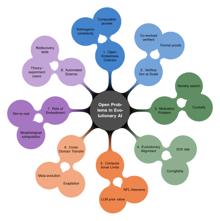
Historical Timeline
The story of evolutionary computation spans nearly two centuries, from Darwin's foundational insight to the modern synthesis of large language models and evolutionary search. The timeline below traces the major milestones, organising them into four overlapping eras: the Foundations (1859–1975), the Classical Period (1975–2000), the Quality-Diversity Revolution (2000–2020), and the LLM-Evolution Synthesis (2020–present).
Era I: Foundations (1859–1975)
Historical Note.
1859 – Darwin's On the Origin of Species. Charles Darwin publishes the foundational text of evolutionary biology, introducing the principles of variation, inheritance, and natural selection. Although Darwin knew nothing of genetics or computation, his framework, a population of diverse solutions undergoing selection pressure, would become the template for all subsequent evolutionary algorithms.
Historical Note.
1930s – The Modern Synthesis. Ronald Fisher, J.B.S. Haldane, and Sewall Wright unify Darwinian selection with Mendelian genetics, creating the mathematical framework of population genetics. Fisher's Fundamental Theorem of Natural Selection (1930) establishes that the rate of increase in mean fitness is proportional to the genetic variance in fitness, a result that foreshadows the diversity-maintenance strategies of modern evolutionary algorithms.
Historical Note.
1953 – Barricelli's numerical evolution. Nils Aall Barricelli, working at the Institute for Advanced Study in Princeton on John von Neumann's computer, conducts what may be the first computer simulation of evolution. His “symbioorganisms” reproduce, mutate, and compete for resources on a one-dimensional grid, a digital precursor to artificial life.
Historical Note.
1962 – Bremermann's optimisation by evolution. Hans-Joachim Bremermann publishes one of the first explicit proposals for using simulated evolution as an optimisation method, applying mutation and selection to parameter vectors in .
Historical Note.
1966 – Fogel's evolutionary programming. Lawrence Fogel introduces evolutionary programming, evolving finite-state machines to predict symbol sequences. Unlike later genetic algorithms, Fogel's approach uses mutation as the sole variation operator (no crossover), emphasising the evolution of behaviour rather than representation.
Historical Note.
1973 – Rechenberg's evolution strategies. Ingo Rechenberg publishes his doctoral thesis on Evolutionsstrategien, introducing the and selection schemes and the crucial concept of self-adaptive mutation step sizes. Rechenberg's -th success rule, which adjusts the mutation step size so that roughly one-fifth of mutations are successful, remains a practical guideline to this day.
Historical Note.
1975 – Holland's genetic algorithms. John Holland publishes Adaptation in Natural and Artificial Systems, introducing the genetic algorithm (GA) with its signature operators: binary encoding, crossover, and mutation. Holland's Schema Theorem provides the first theoretical analysis of why GAs work, arguing that short, low-order, above-average schemata receive exponentially increasing trials, the so-called “building block hypothesis.”
Era II: Classical Period (1975–2000)
Historical Note.
1984 – Axelrod's evolution of cooperation. Robert Axelrod holds a computer tournament for iterated Prisoner's Dilemma strategies, then evolves strategies using a genetic algorithm. The result, that cooperative strategies like Tit-for-Tat can evolve and persist, demonstrates the power of coevolution in game-theoretic settings and inspires decades of research on the evolution of social behaviour.
Historical Note.
1989 – Goldberg's GA bible. David Goldberg publishes Genetic Algorithms in Search, Optimization, and Machine Learning, which becomes the definitive reference for GA practitioners and introduces a generation of engineers and scientists to evolutionary computation.
Historical Note.
1990 – Hillis's host–parasite coevolution. W. Daniel Hillis demonstrates that co-evolving “parasites” (adversarial test cases) alongside “hosts” (sorting networks) dramatically improves the quality of evolved solutions. The sorting networks evolved by Hillis's system are smaller than any previously found by human or machine. This work establishes coevolution as a fundamental technique in evolutionary computation.
Historical Note.
1992 – Koza's genetic programming. John Koza publishes Genetic Programming, extending evolutionary computation from fixed-length strings to tree-structured programs. For the first time, evolution operates directly in the space of executable code, a paradigm that would find its fullest expression three decades later in LLM-guided program evolution.
Historical Note.
1994 – Sims's virtual creatures. Karl Sims evolves virtual creatures with co-adapted morphologies and neural network controllers in a 3D physics simulation. Creatures learn to walk, swim, and compete for resources, developing body plans of stunning creativity. The work remains one of the most compelling demonstrations of evolutionary design.
Historical Note.
1994 – Potter and De Jong's cooperative coevolution. Mitchell Potter and Kenneth De Jong introduce cooperative coevolutionary algorithms, decomposing a problem into subcomponents evolved in separate populations that must cooperate to solve the overall problem. This framework becomes the standard approach for large-scale evolutionary optimisation.
Historical Note.
1997 – Rosin and Belew's Hall of Fame. Christopher Rosin and Richard Belew introduce the Hall of Fame method for coevolutionary algorithms, maintaining an archive of past champions to prevent cyclic dynamics and ensure monotonic progress.
Historical Note.
1997 – Wolpert and Macready's No Free Lunch. David Wolpert and William Macready prove the No Free Lunch theorems for search and optimisation: averaged over all possible objective functions, no algorithm outperforms random search. The theorems sharpen the question of which problem structures make evolutionary algorithms effective, launching a rich theoretical research programme.
Historical Note.
1998 – Banzhaf et al.'s Genetic Programming textbook. Wolfgang Banzhaf, Peter Nordin, Robert Keller, and Frank Francone publish a comprehensive textbook that establishes genetic programming as a mature discipline, covering theory, practice, and applications ranging from symbolic regression to circuit design.
Historical Note.
1999 – Grammatical evolution. Conor Ryan, J.J. Collins, and Michael O'Neill introduce grammatical evolution, which maps variable-length integer strings to programs via a user-specified BNF grammar. This decouples the genotype representation from the phenotype syntax, enabling evolution to respect the grammar of the target language by construction.
Era III: Quality–Diversity Revolution (2000–2020)
Historical Note.
2002 – Stanley and Miikkulainen's NEAT. Kenneth Stanley and Risto Miikkulainen introduce NeuroEvolution of Augmenting Topologies (NEAT), which evolves both the weights and topology of neural networks using speciation and complexification. NEAT demonstrates that starting from minimal networks and incrementally adding complexity is far more effective than evolving fixed-topology networks.
Historical Note.
2002 – Deb et al.'s NSGA-II. Kalyanmoy Deb and colleagues publish the Non-dominated Sorting Genetic Algorithm II (NSGA-II), which becomes the most widely used multi-objective evolutionary algorithm. Its efficient non-dominated sorting and crowding distance mechanisms make Pareto-front approximation practical for real-world problems.
Historical Note.
2008 – Stanley and Miikkulainen's HyperNEAT. HyperNEAT extends NEAT by using compositional pattern-producing networks (CPPNs) as indirect encodings for neural network connectivity. This enables the evolution of large-scale networks with regular, repeating patterns, bridging evolutionary search and deep learning architectures.
Historical Note.
2011 – Lehman and Stanley's novelty search. Joel Lehman and Kenneth Stanley introduce novelty search, which abandons the fitness function entirely and instead selects for behavioural novelty. The counterintuitive finding, that ignoring the objective can lead to better solutions than optimising for it, challenges the foundations of optimisation-based search and opens the door to quality-diversity methods.
Historical Note.
2015 – Mouret and Clune's MAP-Elites. Jean-Baptiste Mouret and Jeff Clune introduce the Multi-dimensional Archive of Phenotypic Elites (MAP-Elites), which maintains a grid of the highest-performing solution for each cell in a user-defined behavioural descriptor space. MAP-Elites becomes the canonical quality-diversity algorithm, finding applications in robotics, game design, and aerodynamic optimisation.
Historical Note.
2017 – Salimans et al.'s evolution strategies for RL. Tim Salimans and colleagues at OpenAI demonstrate that simple evolution strategies, scaling to thousands of parallel workers, can solve reinforcement learning benchmarks competitively with gradient-based methods. The work reignites interest in evolutionary approaches for deep RL and highlights the embarrassingly parallel nature of evolutionary computation.
Historical Note.
2019 – Stanley et al.'s open-endedness manifesto. Kenneth Stanley, Joel Lehman, and Lisa Soros publish a landmark paper arguing that the greatest challenge in AI is open-ended search: the creation of algorithms that can endlessly generate novel, increasingly complex artefacts, much as biological evolution has done on Earth. The paper catalyses a new research community focused on open-ended evolution.
Historical Note.
2019 – POET: Paired Open-Ended Trailblazer. Rui Wang and colleagues introduce POET, which co-evolves both the environments and the agents that solve them, demonstrating that open-ended coevolution can discover solutions that are unreachable by optimising a fixed objective.
Historical Note.
2015–2020 – Quality-diversity at scale. The quality-diversity paradigm matures rapidly. Cully et al. demonstrate that MAP-Elites can enable a damaged hexapod robot to adapt in under two minutes by drawing on a pre-computed repertoire of diverse gaits [29]. Gravina et al. extend QD to procedural content generation for video games. Fontaine and Nikolaidis introduce differentiable quality-diversity (DQD), combining gradient-based optimisation with MAP-Elites to achieve orders-of-magnitude speedups on continuous domains.
Era IV: The LLM–Evolution Synthesis (2020–Present)
Historical Note.
2023 – Lehman et al.'s Evolution Through Large Models. Joel Lehman, Jonathan Gordon, Shyamal Patel, and colleagues publish “Evolution Through Large Models” (ELM), demonstrating that large language models can serve as mutation and crossover operators in evolutionary algorithms. The LLM's knowledge of code structure and semantics enables it to make “intelligent” mutations that would be astronomically unlikely under random perturbation. This paper marks the beginning of the LLM-evolution synthesis.
Historical Note.
2023 – Romera-Paredes et al.'s FunSearch. Working at Google DeepMind, Bernardino Romera-Paredes and colleagues introduce FunSearch, which uses an LLM to evolve programs that solve hard combinatorial problems. FunSearch discovers new constructions for the cap set problem that improve on the best known results in extremal combinatorics, marking the first time an LLM-evolutionary system produces genuinely novel mathematical knowledge.
Historical Note.
2024 – The AI Scientist. Chris Lu, Cong Lu, and colleagues introduce the AI Scientist, a system that autonomously generates research ideas, implements experiments, analyses results, and writes scientific papers. While operating within constrained domains, it demonstrates the feasibility of automated scientific discovery through evolutionary exploration of the idea space.
Historical Note.
2024 – ADAS: Automated Design of Agentic Systems. Shengran Hu and colleagues introduce ADAS, which uses an LLM to evolve the code defining entire agentic systems, including their prompts, tool use, and control flow, optimising for performance on downstream tasks. ADAS demonstrates that evolution can operate at the level of entire AI architectures.
Historical Note.
2025 – AlphaEvolve. Google DeepMind releases AlphaEvolve, scaling LLM-guided program evolution to large codebases and complex optimisation problems. AlphaEvolve discovers improvements to hash functions, matrix multiplication algorithms, and scheduling policies used in Google's production infrastructure, demonstrating that evolved code can outperform decades of human engineering.
Historical Note.
2025 – The Cambrian explosion. A rapid proliferation of LLM-evolutionary systems emerges: GEPA (Guided Evolution of Prompts and Agents) applies multi-objective evolution to software engineering tasks; ShinkaEvolve combines Japanese-inspired island model evolution with LLM mutation; DRQ (Digital Red Queen) evolves Core War warriors in an endless adversarial arms race; AdaEvolve introduces hierarchical UCB-based compute allocation; EvoX provides a scalable GPU-accelerated framework for evolutionary computation; and CALM (Coevolutionary Alignment through Language Models) addresses the alignment problem in self-modifying evolutionary systems. The field enters what many researchers call a “Cambrian explosion” of evolutionary AI methods.
Historical Note.
2025 – Theoretical advances. Alongside the engineering systems, 2025 sees significant theoretical progress. New convergence results for LLM-guided evolutionary algorithms establish conditions under which population-based LLM search provably outperforms single-query LLM inference. Information-theoretic analyses quantify the “prior advantage” that LLMs bring to evolutionary search, connecting to the No Free Lunch framework (Open Problem 5: Computational Limits of Evolutionary Search). Formal definitions of open-endedness, building on the proposals in Conjecture 5, are debated at major conferences, with no consensus yet reached.
Remark 43.
The accelerating pace of the timeline is itself noteworthy. The Foundations era spans over a century (1859–1975). The Classical era spans a quarter-century (1975–2000). The Quality-Diversity era spans two decades (2000–2020). And the LLM-Evolution era has produced more landmark systems in its first five years (2020–2025) than the entire Classical era. Whether this acceleration is sustainable or represents a temporary burst of activity driven by the novelty of LLM integration remains to be seen.
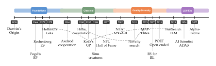
Remark 44.
A striking pattern emerges from the timeline: each era is characterised by a relaxation of constraints on what evolution can modify. In the Foundations era, evolution operated on fixed-length binary strings. In the Classical era, it extended to variable-length programs and morphologies. In the Quality-Diversity era, the notion of “solution” expanded to include entire behavioural repertoires. In the LLM era, evolution can modify programs, prompts, architectures, and even the evolutionary process itself. If this trend continues, the next era may see evolution operating on the very foundations of computation: the languages, logics, and representational systems in which solutions are expressed.
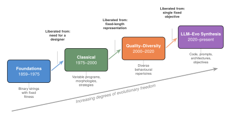
Exercises
The exercises below are organised in roughly increasing order of difficulty. Exercises Exercise 84–Exercise 87 cover classical evolutionary algorithm design. Exercises Exercise 88–Exercise 90 require implementing coevolutionary and quality-diversity methods. Exercises Exercise 91–Exercise 93 address the design of LLM-evolutionary systems. Exercises Exercise 94–Exercise 101 involve mathematical proofs. The final five exercises (marked as Challenge) are open-ended research-level problems.
Exercise 84 (GA Fundamentals).
Consider a genetic algorithm operating on binary strings of length with population size , tournament selection with tournament size , single-point crossover with probability , and bit-flip mutation with probability .
Compute the expected number of bits flipped per offspring under mutation. What is the probability that an offspring is identical to its parent (i.e., no bits are flipped)?
The OneMax fitness function assigns . Derive the expected fitness improvement per generation when the population mean fitness is (half the optimum). Hint: Consider the selection differential under tournament selection and the effect of mutation.
Implement this GA and run it on OneMax for . Plot the number of generations to reach the optimum versus . Does the scaling appear polynomial or exponential? Compare with the known result that the -EA solves OneMax in expected evaluations.
Modify the fitness function to . How does the convergence behaviour change, and why?
Exercise 85 (Schema Theorem Analysis).
Let be a schema of length , order , and defining length (the distance between the first and last fixed positions).
In a population of binary strings of length , suppose strings match schema at generation , and their average fitness is while the population average fitness is . Using Holland's Schema Theorem, compute a lower bound on assuming single-point crossover with probability and bit-flip mutation with probability .
Explain why the Schema Theorem provides only a lower bound, not an exact prediction. What phenomena does it fail to account for?
The “building block hypothesis” states that GAs work by combining short, low-order, above-average schemata into complete solutions. Construct an explicit example of a fitness function where this hypothesis fails. Hint: consider a deceptive function where the optimal building blocks, when combined, lead away from the global optimum.
Exercise 86 (Evolution Strategies).
Consider the -ES applied to minimising for with , , and .
Each offspring is generated as where . Derive the expected fitness of the best offspring as a function of and .
Implement the CMA-ES algorithm (see Evolution Strategies) and apply it to the Rosenbrock function for . Plot convergence curves and report the number of function evaluations to reach .
Compare the performance of CMA-ES with (i) a standard -ES with isotropic mutation and (ii) gradient descent. For which values of does each method dominate?
Exercise 87 (Fitness Sharing and Niching).
The fitness sharing mechanism modifies an individual's fitness by dividing it by its niche count: where is the sharing function with parameters (sharing radius) and (shape parameter, typically ).
Consider a fitness landscape with two peaks of height and at positions and in , with Gaussian profiles of width . With and , compute the shared fitness of an individual at when other individuals are also at . For what value of does the shared fitness at equal the shared fitness of a lone individual at ?
Implement a GA with fitness sharing and apply it to the function above. Verify that the population distributes itself across both peaks in a ratio proportional to their heights.
Explain why fitness sharing can fail in high-dimensional search spaces. What is the relationship between the sharing radius and the dimensionality of the search space?
Exercise 88 (Coevolutionary Algorithm Implementation).
Implement a competitive coevolutionary algorithm for the game of Iterated Prisoner's Dilemma (IPD).
Represent strategies as lookup tables: given the history of the last moves, the strategy specifies whether to cooperate or defect. How many entries does the lookup table have? Include an initial move for the first rounds.
Implement two coevolutionary approaches: enumerate[(i)]
Competitive coevolution: a single population where fitness is determined by round-robin tournaments.
Hall of Fame: same as (i), but each individual also plays against the best individual from every previous generation. enumerate
Run both approaches for 500 generations and compare: (i) the dominant strategies that emerge, (ii) whether cycling occurs (cooperative strategies give way to exploiters, which give way to retaliators, and so on), and (iii) the effect of the Hall of Fame on stability.
Analyse the evolutionary dynamics using a payoff matrix. Let (mutual cooperation), (temptation), (sucker's payoff), and (mutual defection). Compute the replicator dynamics for a population with three strategy types: Always-Cooperate, Always-Defect, and Tit-for-Tat. Find all fixed points and determine their stability.
Exercise 89 (Red Queen Dynamics).
Consider a simplified host–parasite coevolutionary system where hosts and parasites are each represented by binary strings of length . A host “survives” against a parasite if the Hamming distance ; otherwise the parasite “infects” the host.
For random binary strings of length , compute the probability that . Use the binomial distribution and verify your answer empirically.
Implement the coevolutionary system with separate host and parasite populations (size 50 each), tournament selection, uniform crossover, and bit-flip mutation. Track the population-level Hamming distance between hosts and parasites over 1000 generations.
Does the system exhibit Red Queen dynamics (continuous adaptation without net progress)? Plot the mean fitness of both populations over time. Do you observe oscillations?
Modify the system to use Hillis's approach: hosts are sorting networks and parasites are input sequences that the networks must sort. Describe (in pseudocode) how fitness is defined for both hosts and parasites.
Exercise 90 (MAP-Elites Implementation).
Implement the MAP-Elites algorithm for a robot arm reaching task.
Consider a planar robot arm with joints, each with angle . The end-effector position is where for all . The fitness is the negative distance to a target point . Define a 2D behavioural descriptor space using the position of the third joint.
Implement MAP-Elites with a grid over the behavioural descriptor space. Use Gaussian mutation of joint angles with . Run for evaluations and visualise the resulting archive as a heatmap.
Compute the QD-score (sum of fitnesses across all filled cells) and the coverage (fraction of cells filled) as functions of the number of evaluations.
Compare MAP-Elites with a standard GA that optimises fitness alone. Does MAP-Elites find the global optimum as quickly? Does it find solutions that the GA misses?
Exercise 91 (LLM-Evolutionary Loop Design).
Design (on paper or in code) an LLM-evolutionary loop for evolving Python functions that compute the -th Fibonacci number.
Define the solution representation (Python function signature), the fitness function (correctness on test cases + execution speed), and the prompt template for LLM-guided mutation.
Design three types of LLM-guided mutation operators: (i) point mutation (small local changes), (ii) semantic crossover (combining ideas from two parent functions), and (iii) radical mutation (requesting a fundamentally different algorithmic approach). Write the prompt template for each.
Describe an island model architecture for this system: how many islands, what migration policy, and how to balance exploitation (refining fast implementations) with exploration (discovering novel algorithms like matrix exponentiation or fast doubling).
What are the risks of this approach? Can the LLM generate code that is correct on test cases but incorrect in general (e.g., due to integer overflow)? How would you mitigate this risk?
Exercise 92 (FunSearch-Style Problem Solving).
Consider the problem of finding large cap sets in (sets of vectors in such that no three vectors form an arithmetic progression).
For , the search space has elements. Write a verifier function that checks whether a given subset is a cap set.
The known maximum cap set size for is 20. Design a fitness function that rewards both the size of the cap set and partial progress (e.g., having few arithmetic progressions among the selected vectors).
Describe how you would prompt an LLM to generate a priority function that assigns priorities to vectors, such that greedily selecting vectors in order of decreasing priority (while maintaining the cap set property) yields a large cap set. This is the approach used by FunSearch.
Discuss why evolving the priority function (an indirect representation) is more effective than evolving the cap set directly (a direct representation). Connect your answer to the concept of search space smoothness.
Exercise 93 (Verification System Design).
Design a multi-level verification system for an LLM-evolutionary loop that evolves sorting algorithms.
Level 1 – Syntax check: describe how to verify that evolved code is syntactically valid Python.
Level 2 – Unit tests: design a suite of test cases that covers edge cases (empty list, single element, already sorted, reverse sorted, duplicates, large inputs). How many test cases are needed for reasonable confidence?
Level 3 – Property-based testing: using a framework like Hypothesis (Python), define the key properties that a correct sorting algorithm must satisfy: (i) output is a permutation of input, (ii) output is non-decreasing, (iii) output length equals input length. Write the property specifications.
Level 4 – Formal verification: describe how you would express the correctness of a sorting algorithm in a formal logic (e.g., Hoare logic). What are the pre- and post-conditions? What loop invariants would you need?
Estimate the computational cost of each verification level as a function of the code length and the input size . At what point does verification become the bottleneck in the evolutionary loop?
Exercise 94 (Fitness Landscape Analysis).
Let be a fitness function. The fitness landscape graph has vertex set and edge set (i.e., the Boolean hypercube).
Prove that if is a linear function ( for some and ), then has exactly one local optimum, which is also the global optimum.
A function is -epistatic if it can be written as where each subset has and denotes the restriction of to the indices in . Prove that a -epistatic function has at most local optima. Hint: use the decomposition to show that each local optimum is determined by the local optima of the subfunctions.
The autocorrelation of under random walk on the hypercube is where is a random walk that flips one random bit per step. Compute for the function and interpret the result in terms of landscape “ruggedness.”
Exercise 95 (Selection Pressure Analysis).
Consider three selection mechanisms applied to a population of individuals with fitness values :
Proportional selection: individual is selected with probability .
Tournament selection with tournament size .
truncation selection: the best individuals survive.
For a linear fitness distribution , compute the expected number of copies of the best individual under each selection mechanism. Set for tournament selection and , for truncation selection.
The selection intensity is defined as where is the mean fitness of selected individuals, is the population mean, and is the fitness standard deviation. Compute for each mechanism using the linear fitness distribution.
Explain the trade-off between selection intensity and population diversity. Under which conditions does high selection intensity lead to premature convergence?
Exercise 96 (Open-Endedness Metrics).
Consider a simple artificial life system where agents are represented by binary strings of length that move on a grid, consume resources, and reproduce when their energy exceeds a threshold.
Define three concrete metrics for measuring “open-endedness” in this system: (i) phenotypic diversity (number of distinct phenotypes observed), (ii) activity statistics (rate of novel phenotype generation over a sliding window), and (iii) complexity growth (mean Lempel–Ziv complexity of agent genomes over time).
For each metric, describe a scenario where the metric incorrectly classifies a system as open-ended. What failure mode does each metric have?
Propose a composite metric that combines all three. What weights or combination rule would you use, and why?
Relate your metrics to the three conditions in Conjecture 5. Which conditions does each metric address?
Exercise 97 (Safety of Self-Modifying Systems).
Consider an evolutionary system that evolves Python programs and has the ability to modify its own mutation operator (i.e., the prompt template used to instruct the LLM).
List at least five specific ways this system could behave unsafely. For each, describe the mechanism by which the unsafe behaviour could arise.
For each unsafe behaviour, propose a concrete mitigation. Classify each mitigation as either (i) prevention (making the behaviour impossible), (ii) detection (identifying the behaviour when it occurs), or (iii) correction (reverting the system after the behaviour is detected).
The system evolves a mutation operator that produces code with very high fitness on the test suite but that also writes to the filesystem. Design a sandboxing mechanism that prevents this while still allowing the evolved code to perform legitimate I/O (e.g., reading input from stdin).
Formally model the system as a Markov chain where the state includes both the population and the mutation operator. Under what conditions on the transition probabilities is the system guaranteed to remain in the set of “safe” states?
Exercise 98 (Multi-Objective Evolutionary Optimisation).
Consider the bi-objective minimisation problem: where .
Analytically derive the Pareto front for this problem. Show that the Pareto-optimal solutions lie on the line segment connecting and . Hint: parametrise the Pareto front as for and verify that no solution off this segment dominates any solution on it.
Implement NSGA-II with population size , SBX crossover (), and polynomial mutation (). Run for 200 generations and plot the evolved Pareto front approximation against the analytical solution.
Compute the hypervolume indicator of the evolved front with reference point . How does this metric change over generations?
Extend the problem to three objectives by adding . How does the dimensionality of the Pareto front change? Does NSGA-II scale well to three objectives, or would you need a many-objective algorithm like NSGA-III?
Exercise 99 (Island Model Parallelism).
Implement an island model evolutionary algorithm for the Rastrigin function with .
Create islands, each running a standard GA with population size 50. Implement three migration topologies: (i) ring (each island sends migrants to its neighbour), (ii) fully connected (each island sends migrants to all others), and (iii) random (each island sends migrants to a randomly chosen island).
For each topology, experiment with migration rates (fraction of population migrated) and migration intervals (generations between migrations). Which combination yields the best performance?
Compare the island model with a single panmictic population of size . Under what conditions does the island model find better solutions?
Analyse the diversity dynamics: measure the mean pairwise Euclidean distance within and between islands over time. How does migration rate affect inter-island diversity?
Exercise 100 (Comparative Analysis).
Fill in the following table comparing five LLM-evolutionary systems discussed in this chapter. For each system, identify the representation, mutation mechanism, selection strategy, evaluation method, and key result.
| System | Repr. | Mutation | Selection | Evaluation | Key Result |
| FunSearch | |||||
| AlphaEvolve | |||||
| ELM | |||||
| AI Scientist | |||||
| ADAS |
For each entry, provide a one-sentence description. Then write a short essay (300–500 words) comparing and contrasting the five systems along the dimensions in the table.
Exercise 101 (NFL Theorem Extension).
The No Free Lunch theorem states that for any algorithm and any performance measure , for any algorithm , where is the set of all functions from to .
Prove this theorem for the case where , , and counts the number of evaluations to find the global maximum.
The NFL theorem assumes a uniform prior over all possible fitness functions. Suppose instead we have a prior over that assigns higher probability to “smooth” functions (functions with high autocorrelation , as defined in Exercise 94). Show that under this prior, a -EA outperforms random search in expectation.
Discuss the implications of part (b) for LLM-guided evolution. The LLM's prior over programs is highly non-uniform: it assigns high probability to “natural” or “reasonable” programs. How does this relate to the NFL theorem and the effectiveness of LLM-guided search?
Challenge 1 (Design an Open-Ended Evolution System).
Design and implement a minimal open-ended evolution system that satisfies at least two of the three conditions in Conjecture 5.
Choose a representation for agents (e.g., neural networks, programs, cellular automata rules) and a simulated environment that supports interaction and resource competition.
Implement the system and run it for at least 10,000 generations. Measure all three open-endedness metrics from Exercise 96.
Does your system exhibit unbounded novelty? Unbounded complexity? Ecological non-collapse? If not, identify the bottleneck and propose modifications.
Compare your system with Avida, Tierra, or Lenia on the same metrics. What features of these established systems contribute most to their open-endedness?
This exercise is suitable for a course project spanning several weeks.
Challenge 2 (Evolve a Novel Algorithm).
Using an LLM-evolutionary loop (either implemented from scratch or using an existing framework), evolve a sorting algorithm that is not a known algorithm (i.e., not insertion sort, merge sort, quicksort, heapsort, etc.).
Design the evaluation pipeline: correctness tests, performance benchmarks on random, sorted, reverse-sorted, and nearly-sorted inputs of varying sizes.
Run the evolutionary loop for at least 500 generations with a population of at least 20 individuals.
Analyse the best evolved algorithm. Is it genuinely novel, or is it a recombination of known algorithms? How do you determine novelty?
Measure the time complexity of the evolved algorithm empirically. Can you prove its worst-case complexity?
Reflect on the role of the LLM: did it contribute domain knowledge (e.g., divide-and-conquer strategies) or primarily syntactic variation?
Challenge 3 (Coevolutionary Alignment Monitor).
Design a coevolutionary system where one population evolves solutions and another population evolves alignment monitors that detect unsafe or misaligned behaviour.
Define a concrete domain: for example, evolving trading strategies where “alignment” means avoiding market manipulation, or evolving text generators where “alignment” means avoiding toxic content.
Define fitness functions for both populations. Solution fitness should reward task performance; monitor fitness should reward detection of alignment violations.
Analyse the game-theoretic equilibria of your system. Under what conditions does the coevolutionary dynamic converge to aligned solutions paired with effective monitors?
Implement the system and test whether the monitors generalise: do monitors evolved against one population of solutions detect alignment violations in a held-out population?
Challenge 4 (Information-Theoretic Analysis of LLM Mutation).
Provide a formal information-theoretic analysis of LLM-guided mutation versus random mutation.
Model the LLM as a conditional distribution where is the parent solution, is the offspring, and is the prompt context. Model random mutation as .
Define the mutation information gain as the mutual information under each mutation model, where is the fitness function. Argue that when the LLM has learned the structure of the fitness landscape.
Under a Gaussian fitness landscape model , compute explicitly. What assumptions about are needed for to be significantly larger?
Discuss the limits of this analysis. When might LLM-guided mutation provide less information than random mutation?
Challenge 5 (Automated Scientific Discovery Testbed).
Build a minimal testbed for automated scientific discovery using coevolutionary methods.
Choose a domain where ground truth is known: for example, rediscovering the relationship from simulated force-acceleration data, or rediscovering Ohm's law from circuit simulations.
Implement a coevolutionary system with two populations: (i) theory generators that propose symbolic expressions (e.g., using genetic programming), and (ii) experiment designers that choose which data points to collect next (active learning).
The experiment designers' fitness should be the information gain: how much the experiment discriminates between competing theories. The theory generators' fitness should be the predictive accuracy on collected data.
Run the system and analyse: how many experiments does it need to rediscover the ground-truth law? How does this compare to random experimentation?
Extend to a domain where the ground truth is not known. What changes in the methodology are needed?
This exercise is suitable for a master's thesis project.
Challenge 6 (Scaling Laws for Evolutionary Search).
Neural scaling laws relate model performance to compute, data, and parameters via power laws. Investigate whether analogous scaling laws exist for evolutionary search.
Choose a family of optimisation problems parametrised by difficulty (e.g., the NK landscape model with varying and , or the Travelling Salesman Problem with varying number of cities).
For each problem size, run an evolutionary algorithm with varying population sizes and varying computational budgets (number of fitness evaluations ).
Plot the best fitness achieved as a function of and on log-log axes. Does a power law provide a good fit? How does the exponent depend on problem difficulty?
Repeat the analysis with an LLM-guided evolutionary loop. Does LLM guidance change the scaling exponent? Is the improvement multiplicative (shifting the curve) or does it change the slope?
Discuss whether evolutionary scaling laws, if they exist, have the same implications as neural scaling laws for resource allocation. Can we predict the computational budget needed to solve a problem of given difficulty?
Chapter Summary
This chapter has journeyed from the foundations of evolutionary computation to the frontiers of autonomous AI-driven discovery. Let us retrace the path, highlighting the key ideas and their connections.
Foundations of evolutionary search.
We began with the core abstraction shared by all evolutionary algorithms: a population of candidate solutions undergoes variation (mutation and crossover), evaluation (fitness assessment), and selection (survival of the fittest). We formalised this cycle mathematically, defining fitness landscapes, selection operators, and the schema-theoretic analysis that provides the classical explanation for why genetic algorithms work (Biological Foundations). Evolution strategies, with their elegant self-adaptation of mutation parameters through CMA-ES, showed that the evolutionary framework extends naturally to continuous optimisation in (Evolution Strategies).
Coevolution: when the landscape fights back.
The introduction of coevolution transformed evolutionary computation from an optimisation technique into a framework for modelling adaptive systems. Competitive coevolution, exemplified by Hillis's host–parasite sorting networks, demonstrated that antagonistic interactions can drive solutions beyond the reach of fixed-objective optimisation (Competitive Coevolution). Cooperative coevolution decomposed complex problems into co-adapted modules, while the theory of evolutionary game dynamics provided the mathematical tools to analyse coevolutionary stability and cycling (Cooperative Coevolution).
Beyond fitness: quality, diversity, and novelty.
The quality-diversity revolution challenged the assumption that evolution should optimise a single objective. Novelty search demonstrated that abandoning the fitness function entirely can paradoxically improve performance on deceptive landscapes (Novelty Search). MAP-Elites and its descendants provided a practical framework for illuminating the space of possible solutions, producing diverse repertoires that are valuable for downstream adaptation (MAP-Elites).
The LLM-evolution synthesis.
The convergence of large language models and evolutionary algorithms represents, in our view, the most consequential development in the field since its inception. By replacing random mutation with intelligent mutation guided by an LLM's knowledge of code structure, program semantics, and domain conventions, systems like FunSearch and AlphaEvolve have achieved results that were inconceivable under classical evolutionary computation (AlphaEvolve: Open-Ended Algorithmic Discovery). The LLM serves as a learned prior over the space of solutions, dramatically narrowing the search space while preserving the exploration benefits of population-based methods.
Autonomous discovery and the AI Scientist.
The AI Scientist and ADAS frameworks showed that evolution can operate not just on solutions but on entire research programmes and agentic architectures (The AI Scientist: Autonomous Research Agents). These systems close the loop between hypothesis generation, experimental validation, and theory refinement, pointing towards a future where AI systems conduct genuine scientific research with minimal human oversight.
Open-ended evolution: the grand challenge.
The deepest aspiration of evolutionary AI is open-ended evolution: the creation of systems that produce an unbounded stream of increasingly complex and novel artefacts, mirroring the creative power of biological evolution on Earth. We formalised this aspiration in Conjecture 5 and surveyed the barriers to achieving it, including the verification bottleneck, the motivation problem, and the alignment challenge (Open Problems and Future Directions).
Safety and alignment.
Throughout the chapter, we emphasised that the power of evolutionary self-modification demands commensurate safeguards. The alignment instability conjecture (Conjecture 7) warns that self-modifying systems will inevitably drift from human values unless explicit constraints are maintained. The verification gap (Definition 74) highlights the growing difficulty of certifying evolved solutions as they increase in complexity. These are not hypothetical concerns: as LLM-evolutionary systems move from research prototypes to production deployments, the need for rigorous safety guarantees becomes urgent.
The grand narrative.
Viewed from a distance, the story told in this chapter is one of progressive liberation. Darwin liberated biology from the need for a designer. Holland liberated optimisation from the need for a gradient. Koza liberated evolution from the need for a fixed representation. Stanley and Lehman liberated search from the need for a fixed objective. And the LLM-evolution synthesis is liberating evolution from the need for random mutation, perhaps the last constraint that kept artificial evolution from matching the creative power of its biological counterpart.
Whether this liberation leads to a golden age of automated discovery or to systems that outpace our ability to understand and control them depends on the choices we make in the coming years. The open problems of Open Problems and Future Directions are not merely academic puzzles: they are the research programme on which the responsible development of evolutionary AI depends.
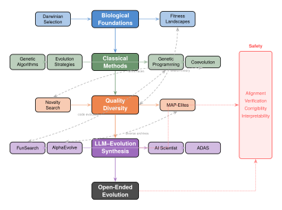
Connections to other chapters.
The ideas developed in this chapter intersect with numerous topics covered elsewhere in this book. The evolution of neural architectures connects directly to the neural architecture search methods of 30, where evolutionary approaches like NEAT provide an alternative to gradient-based NAS. The coevolutionary training of generators and discriminators echoes the adversarial dynamics of GANs (9), where the generator–discriminator interplay can be viewed as a special case of competitive coevolution. The use of LLMs as mutation operators draws on the autoregressive generation techniques of ch:transformers, and the quality-diversity methods that illuminate behavioural spaces have natural connections to the latent space exploration techniques in variational autoencoders (15).
Perhaps most profoundly, the open-endedness criterion (Conjecture 5) connects to fundamental questions in information theory (ch:info-theory): can we use information-theoretic quantities to measure and certify the ongoing novelty production of an evolutionary system? The answer to this question may lie at the intersection of Kolmogorov complexity, rate-distortion theory, and the mathematics of dynamical systems.
A closing reflection.
Biological evolution has had nearly four billion years to demonstrate its creative power, producing everything from archaebacteria to the human neocortex, from the camouflage of the cuttlefish to the echolocation of the bat. Artificial evolution has had barely fifty years and is already discovering novel mathematics, optimising production infrastructure, and taking its first steps towards autonomous science. The gap between these two timescales is itself a measure of how far we have come and how much further we might go.
The detective story that began with Darwin's insight into natural selection has led us to a frontier where evolution and intelligence are no longer separate phenomena but deeply intertwined partners in the search for knowledge. The next chapter of this story will be written not by nature alone, but by the evolutionary systems we create, systems that, if we build them wisely, may one day surprise even their creators.
Key Idea.
The central lesson of this chapter can be stated in a single sentence: evolution is most powerful when it evolves not just solutions but the search process itself. From self-adapting mutation rates in CMA-ES to self-modifying objectives in open-ended evolution to LLM-guided mutation that leverages the entire history of human programming, the most transformative advances in evolutionary computation have always come from giving evolution more degrees of freedom. The challenge for the next generation of researchers is to expand these degrees of freedom while maintaining the safety, interpretability, and alignment guarantees that responsible deployment demands.
[heading=subbibliography]
References
-
The Origins of Order: Self-Organization and Selection in Evolution
BibTeX
@book{kauffman1993origins, author = {Kauffman, Stuart A.}, title = {The Origins of Order: Self-Organization and Selection in Evolution}, publisher = {Oxford University Press}, year = {1993} }Book
-
Evolutionsstrategie: Optimierung technischer Systeme nach Prinzipien der biologischen Evolution
BibTeX
@book{rechenberg1973evolution, author = {Rechenberg, Ingo}, title = {Evolutionsstrategie: Optimierung technischer Systeme nach Prinzipien der biologischen Evolution}, publisher = {Frommann-Holzboog}, year = {1973} }Book
-
Numerische Optimierung von Computer-Modellen mittels der Evolutionsstrategie
BibTeX
@book{schwefel1977evolution, author = {Schwefel, Hans-Paul}, title = {Numerische Optimierung von Computer-Modellen mittels der Evolutionsstrategie}, publisher = {Birkh{\"a}user}, year = {1977} }Book
-
Adaptation in Natural and Artificial Systems
BibTeX
@book{holland1975adaptation, title={Adaptation in Natural and Artificial Systems}, author={Holland, John H.}, publisher={University of Michigan Press}, address={Ann Arbor, MI}, year={1975} }Book
-
Genetic Programming: On the Programming of Computers by Means of Natural Selection
BibTeX
@book{koza1992genetic, title={Genetic Programming: On the Programming of Computers by Means of Natural Selection}, author={Koza, John R.}, publisher={MIT Press}, address={Cambridge, MA}, year={1992} }Book
-
Evolving Neural Networks through Augmenting Topologies
BibTeX
@article{stanley2002neat, title={Evolving Neural Networks through Augmenting Topologies}, author={Stanley, Kenneth O. and Miikkulainen, Risto}, journal={Evolutionary Computation}, volume={10}, number={2}, pages={99--127}, year={2002} }Journal article
-
Regularized Evolution for Image Classifier Architecture Search
BibTeX
@inproceedings{real2019regularized, title={Regularized Evolution for Image Classifier Architecture Search}, author={Real, Esteban and Aggarwal, Alok and Huang, Yanping and Le, Quoc V.}, booktitle={Proceedings of the AAAI Conference on Artificial Intelligence}, volume={33}, pages={4780--4789}, year={2019} }Conference paper
-
Abandoning Objectives: Evolution through the Search for Novelty Alone
BibTeX
@article{lehman2011novelty, author = {Lehman, Joel and Stanley, Kenneth O.}, title = {Abandoning Objectives: Evolution through the Search for Novelty Alone}, journal = {Evolutionary Computation}, volume = {19}, number = {2}, pages = {189--223}, year = {2011} }Journal article
-
Evolution Strategies as a Scalable Alternative to Reinforcement Learning
BibTeX
@article{salimans2017evolution, author = {Salimans, Tim and Ho, Jonathan and Chen, Xi and Sidor, Szymon and Sutskever, Ilya}, title = {Evolution Strategies as a Scalable Alternative to Reinforcement Learning}, journal = {arXiv preprint arXiv:1703.03864}, year = {2017} }Journal article
-
Deep Neuroevolution: Genetic Algorithms Are a Competitive Alternative for Training Deep Neural Networks for Reinforcement Learning
BibTeX
@article{such2017deep, author = {Such, Felipe Petroski and Madhavan, Vashisht and Conti, Edoardo and Lehman, Joel and Stanley, Kenneth O. and Clune, Jeff}, title = {Deep Neuroevolution: Genetic Algorithms Are a Competitive Alternative for Training Deep Neural Networks for Reinforcement Learning}, journal = {arXiv preprint arXiv:1712.06567}, year = {2017} }Journal article
-
Evolution through Large Models
BibTeX
@article{lehman2023evolution, author = {Lehman, Joel and Gordon, Jonathan and Jain, Shawn and Ndousse, Kamal and Yeh, Cathy and Stanley, Kenneth O.}, title = {Evolution through Large Models}, journal = {arXiv preprint arXiv:2206.08896}, year = {2023} }Journal article
-
Co-Evolving Parasites Improve Simulated Evolution as an Optimization Procedure
BibTeX
@article{hillis1990coevolving, author = {Hillis, W. Daniel}, title = {Co-Evolving Parasites Improve Simulated Evolution as an Optimization Procedure}, journal = {Physica D}, volume = {42}, pages = {228--234}, year = {1990} }Journal article
-
Evolving Virtual Creatures
BibTeX
@inproceedings{sims1994evolving, author = {Sims, Karl}, title = {Evolving Virtual Creatures}, booktitle = {Proceedings of SIGGRAPH}, pages = {15--22}, year = {1994} }Conference paper
-
Cooperative Coevolution: An Architecture for Evolving Coadapted Subcomponents
BibTeX
@article{potter2000cooperative, author = {Potter, Mitchell A. and De Jong, Kenneth A.}, title = {Cooperative Coevolution: An Architecture for Evolving Coadapted Subcomponents}, journal = {Evolutionary Computation}, volume = {8}, number = {1}, pages = {1--29}, year = {2000} }Journal article
-
Illuminating Search Spaces by Mapping Elites
BibTeX
@article{mouret2015mapelites, author = {Mouret, Jean-Baptiste and Clune, Jeff}, title = {Illuminating Search Spaces by Mapping Elites}, journal = {arXiv preprint arXiv:1504.04909}, year = {2015} }Journal article
-
Quality Diversity: A New Frontier for Evolutionary Computation
BibTeX
@article{pugh2016quality, author = {Pugh, Justin K. and Soros, Lisa B. and Stanley, Kenneth O.}, title = {Quality Diversity: A New Frontier for Evolutionary Computation}, journal = {Frontiers in Robotics and AI}, volume = {3}, pages = {40}, year = {2016} }Journal article
-
Surrogate-Assisted Evolutionary Computation: Recent Advances and Future Challenges
BibTeX
@article{jin2011surrogate, author = {Jin, Yaochu}, title = {Surrogate-Assisted Evolutionary Computation: Recent Advances and Future Challenges}, journal = {Swarm and Evolutionary Computation}, volume = {1}, number = {2}, pages = {61--70}, year = {2011} }Journal article
-
AlphaEvolve: A Coding Agent for Scientific and Algorithmic Discovery
BibTeX
@article{alphaevolve2025, author = {Novikov, Alexander and V{\~u}, Ng{\^a}n and Eisenberger, Marvin and Dupont, Emilien and Huang, Po-Sen and Wagner, Adam Zsolt and Shirobokov, Sergey and Kozlovskii, Borislav and Ruiz, Francisco J. R. and Mehrabian, Abbas and Kumar, M. Pawan and See, Abigail and Chaudhuri, Swarat and Holland, George and Davies, Alex and Nowozin, Sebastian and Kohli, Pushmeet and Balog, Matej}, title = {{AlphaEvolve}: A Coding Agent for Scientific and Algorithmic Discovery}, journal = {arXiv preprint arXiv:2506.13131}, year = {2025} }Journal article
-
Gaussian Elimination is Not Optimal
BibTeX
@article{strassen1969gaussian, author = {Strassen, Volker}, title = {Gaussian Elimination is Not Optimal}, journal = {Numerische Mathematik}, volume = {13}, pages = {354--356}, year = {1969} }Journal article
-
In the Game Called Core War Hostile Programs Engage in a Battle of Bits
BibTeX
@article{dewdney1984, author = {Dewdney, Alexander K.}, title = {In the Game Called {Core War} Hostile Programs Engage in a Battle of Bits}, journal = {Scientific American}, volume = {250}, number = {5}, pages = {14--22}, year = {1984} }Journal article
-
The Theory of Learning in Games
BibTeX
@book{fudenberg1998theory, author = {Fudenberg, Drew and Levine, David K.}, title = {The Theory of Learning in Games}, publisher = {MIT Press}, year = {1998} }Book
-
Adam: A Method for Stochastic Optimization
BibTeX
@article{kingma2015adam, title={Adam: A Method for Stochastic Optimization}, author={Kingma, Diederik P. and Ba, Jimmy}, journal={Proceedings of the International Conference on Learning Representations (ICLR)}, year={2015} }Journal article
-
Speculations Concerning the First Ultraintelligent Machine
BibTeX
@article{good1965speculations, title={Speculations Concerning the First Ultraintelligent Machine}, author={Good, Irving John}, journal={Advances in Computers}, volume={6}, pages={31--88}, year={1965} }Journal article
-
Active Learning Literature Survey
BibTeX
@book{settles2009active, author = {Settles, Burr}, title = {Active Learning Literature Survey}, publisher = {University of Wisconsin--Madison}, year = {2009} }Book
-
The AI Scientist: Towards Fully Automated Open-Ended Scientific Discovery
BibTeX
@article{lu2024aiscientist, author = {Lu, Chris and Lu, Cong and Lange, Robert Tjarko and Foerster, Jakob and Clune, Jeff and Ha, David}, title = {The {AI} Scientist: Towards Fully Automated Open-Ended Scientific Discovery}, journal = {arXiv preprint arXiv:2408.06292}, year = {2024} }Journal article
-
Gaussian Process Optimization in the Bandit Setting: No Regret and Experimental Design
BibTeX
@article{srinivas2010gaussian, author = {Srinivas, Niranjan and Krause, Andreas and Kakade, Sham M. and Seeger, Matthias W.}, title = {Gaussian Process Optimization in the Bandit Setting: No Regret and Experimental Design}, journal = {Proceedings of ICML}, year = {2010} }Journal article
-
CALM: Co-evolution of Algorithms and Language Model for Automatic Heuristic Design
BibTeX
@article{calm2025, author = {Huang, Ziyao and Wu, Weiwei and Wu, Kui and Wang, Jianping and Lee, Wei-Bin}, title = {{CALM}: Co-evolution of Algorithms and Language Model for Automatic Heuristic Design}, journal = {arXiv preprint arXiv:2505.12285}, year = {2025} }Journal article
-
The Selfish Gene
BibTeX
@book{dawkins1976selfish, author = {Dawkins, Richard}, title = {The Selfish Gene}, publisher = {Oxford University Press}, year = {1976} }Book
-
Robots that Can Adapt Like Animals
BibTeX
@article{cully2015robots, author = {Cully, Antoine and Clune, Jeff and Tarapore, Danesh and Mouret, Jean-Baptiste}, title = {Robots that Can Adapt Like Animals}, journal = {Nature}, volume = {521}, pages = {503--507}, year = {2015} }Journal article
-
On the Origin of Species by Means of Natural Selection
BibTeX
@book{darwin1859origin, author = {Darwin, Charles}, title = {On the Origin of Species by Means of Natural Selection}, publisher = {John Murray}, year = {1859}, address = {London} }Book
-
Darwin's Dangerous Idea: Evolution and the Meanings of Life
BibTeX
@book{dennett1995darwins, author = {Dennett, Daniel C.}, title = {Darwin's Dangerous Idea: Evolution and the Meanings of Life}, publisher = {Simon \& Schuster}, year = {1995} }Book
-
The Roles of Mutation, Inbreeding, Crossbreeding, and Selection in Evolution
BibTeX
@article{wright1932roles, author = {Wright, Sewall}, title = {The Roles of Mutation, Inbreeding, Crossbreeding, and Selection in Evolution}, journal = {Proceedings of the Sixth International Congress of Genetics}, volume = {1}, pages = {356--366}, year = {1932} }Journal article
-
The Genetical Theory of Natural Selection
BibTeX
@book{fisher1930genetical, author = {Fisher, Ronald A.}, title = {The Genetical Theory of Natural Selection}, publisher = {Clarendon Press}, year = {1930}, address = {Oxford} }Book
-
A New Evolutionary Law
BibTeX
@article{valen1973new, author = {Van Valen, Leigh}, title = {A New Evolutionary Law}, journal = {Evolutionary Theory}, volume = {1}, pages = {1--30}, year = {1973} }Journal article
-
The Structure of Evolutionary Theory
BibTeX
@book{gould2002structure, author = {Gould, Stephen Jay}, title = {The Structure of Evolutionary Theory}, publisher = {Harvard University Press}, year = {2002} }Book
-
The Neutral Theory of Molecular Evolution
BibTeX
@book{kimura1983neutral, author = {Kimura, Motoo}, title = {The Neutral Theory of Molecular Evolution}, publisher = {Cambridge University Press}, year = {1983} }Book
-
Genetic Algorithms in Search, Optimization, and Machine Learning
BibTeX
@book{goldberg1989genetic, author = {Goldberg, David E.}, title = {Genetic Algorithms in Search, Optimization, and Machine Learning}, publisher = {Addison-Wesley}, year = {1989} }Book
-
Completely Derandomized Self-Adaptation in Evolution Strategies
BibTeX
@article{hansen2001cmaes, author = {Hansen, Nikolaus and Ostermeier, Andreas}, title = {Completely Derandomized Self-Adaptation in Evolution Strategies}, journal = {Evolutionary Computation}, volume = {9}, number = {2}, pages = {159--195}, year = {2001} }Journal article
-
New Methods for Competitive Coevolution
BibTeX
@article{rosin1997newmethods, author = {Rosin, Christopher D. and Belew, Richard K.}, title = {New Methods for Competitive Coevolution}, journal = {Evolutionary Computation}, volume = {5}, number = {1}, pages = {1--29}, year = {1997} }Journal article
-
Solution Concepts in Coevolutionary Search
BibTeX
@inproceedings{ficici2004solution, author = {Ficici, Sevan G.}, title = {Solution Concepts in Coevolutionary Search}, booktitle = {Workshop on Coevolution at GECCO}, year = {2004} }Conference paper
-
FlashAttention: Fast and Memory-Efficient Exact Attention with IO-Awareness
BibTeX
@inproceedings{dao2022flashattention, title={Flash{A}ttention: Fast and Memory-Efficient Exact Attention with {IO}-Awareness}, author={Dao, Tri and Fu, Daniel Y. and Ermon, Stefano and Rudra, Atri and R{\'e}, Christopher}, booktitle={Advances in Neural Information Processing Systems}, volume={35}, year={2022} }Conference paper
-
OpenEvolve: Open-Source LLM-Guided Evolutionary Search
BibTeX
@article{openevolve2025, author = {{OpenEvolve Contributors}}, title = {{OpenEvolve}: Open-Source {LLM}-Guided Evolutionary Search}, journal = {GitHub Repository}, year = {2025} }Journal article
-
CodeEvolve: LLM-Driven Code Evolution
BibTeX
@article{codeevolve2024, author = {{CodeEvolve Contributors}}, title = {{CodeEvolve}: {LLM}-Driven Code Evolution}, journal = {GitHub Repository}, year = {2024} }Journal article
-
Evolving Code with LLM-Guided Semantic Variation
BibTeX
@article{levi2025, author = {Levi, Moshik and others}, title = {Evolving Code with {LLM}-Guided Semantic Variation}, journal = {arXiv preprint}, year = {2025} }Journal article
-
GEPA: Reflective Prompt Evolution Can Outperform Reinforcement Learning
BibTeX
@article{gepa2025, author = {Agrawal, Lakshya A. and Tan, Shangyin and Soylu, Dilara and Ziems, Noah and Khare, Rishi and Opsahl-Ong, Krista and Singhvi, Arnav and Shandilya, Herumb and Ryan, Michael J. and Jiang, Meng and Potts, Christopher and Sen, Koushik and Dimakis, Alexandros G. and Stoica, Ion and Klein, Dan and Zaharia, Matei and Khattab, Omar}, title = {{GEPA}: Reflective Prompt Evolution Can Outperform Reinforcement Learning}, journal = {arXiv preprint arXiv:2507.19457}, year = {2025} }Journal article
-
ShinkaEvolve: Towards Open-Ended and Sample-Efficient Program Evolution
BibTeX
@article{shinkaevolve2025, author = {Imajuku, Yuki and Cetin, Edoardo and Lange, Robert Tjarko}, title = {{ShinkaEvolve}: Towards Open-Ended and Sample-Efficient Program Evolution}, journal = {arXiv preprint arXiv:2509.19349}, year = {2025} }Journal article
-
Finite-Time Analysis of the Multiarmed Bandit Problem
BibTeX
@article{auer2002finite, author = {Auer, Peter and Cesa-Bianchi, Nicol{\`o} and Fischer, Paul}, title = {Finite-Time Analysis of the Multiarmed Bandit Problem}, journal = {Machine Learning}, volume = {47}, number = {2}, pages = {235--256}, year = {2002} }Journal article
-
Mathematical Discoveries from Program Search with Large Language Models
BibTeX
@article{romera2024funsearch, author = {Romera-Paredes, Bernardino and others}, title = {Mathematical Discoveries from Program Search with Large Language Models}, journal = {Nature}, volume = {625}, pages = {468--475}, year = {2024} }Journal article
-
Digital Red Queen: Adversarial Program Evolution in Core War with LLMs
BibTeX
@article{drq2025, author = {Kumar, Akarsh and Bahlous-Boldi, Ryan and Sharma, Prafull and Isola, Phillip and Risi, Sebastian and Tang, Yujin and Ha, David}, title = {Digital Red Queen: Adversarial Program Evolution in Core War with {LLMs}}, journal = {arXiv preprint arXiv:2601.03335}, year = {2025} }Journal article
-
AdaEvolve: Adaptive LLM Driven Zeroth-Order Optimization
BibTeX
@article{adaevolve2025, author = {Cemri, Mert and Agrawal, Shubham and Gupta, Akshat and Liu, Shu and Cheng, Audrey and Mang, Qiuyang and Naren, Ashwin and Erdogan, Lutfi Eren and Sen, Koushik and Zaharia, Matei and Dimakis, Alexandros G. and Stoica, Ion}, title = {{AdaEvolve}: Adaptive {LLM} Driven Zeroth-Order Optimization}, journal = {arXiv preprint arXiv:2602.20133}, year = {2025} }Journal article
-
Automated Design of Agentic Systems
BibTeX
@article{adas2025, author = {Hu, Shengran and Lu, Cong and Clune, Jeff}, title = {Automated Design of Agentic Systems}, journal = {arXiv preprint arXiv:2408.08435}, year = {2025} }Journal article
-
EvoX: Meta-Evolution for Automated Discovery
BibTeX
@article{evox2025, author = {Liu, Shu and Agarwal, Shubham and Maheswaran, Monishwaran and Cemri, Mert and Li, Zhifei and Mang, Qiuyang and Naren, Ashwin and Boneh, Ethan and Cheng, Audrey and Pan, Melissa Z. and Du, Alexander and Keutzer, Kurt and Dimakis, Alexandros G. and Sen, Koushik and Zaharia, Matei and Stoica, Ion}, title = {{EvoX}: Meta-Evolution for Automated Discovery}, journal = {arXiv preprint arXiv:2602.23413}, year = {2025} }Journal article
-
The Lean Theorem Prover (System Description)
BibTeX
@inproceedings{demoura2015lean, author = {de Moura, Leonardo and Kong, Soonho and Avigad, Jeremy and van Doorn, Floris and von Raumer, Jakob}, title = {The {Lean} Theorem Prover (System Description)}, booktitle = {International Conference on Automated Deduction}, pages = {378--388}, year = {2015} }Conference paper
-
LeanCopilot: LLMs as Copilots for Theorem Proving in Lean
BibTeX
@article{leancopilot2024, author = {Song, Peiyang and Yang, Kaiyu and Anandkumar, Anima}, title = {{LeanCopilot}: {LLMs} as Copilots for Theorem Proving in {Lean}}, journal = {arXiv preprint arXiv:2404.12534}, year = {2024} }Journal article
-
AlphaProof: AI Achieves Silver-Medal Standard Solving IMO Problems
BibTeX
@article{alphaproof2024, author = {{Google DeepMind}}, title = {{AlphaProof}: {AI} Achieves Silver-Medal Standard Solving {IMO} Problems}, journal = {Google DeepMind Blog}, year = {2024} }Journal article
-
Why Open-Endedness Matters
BibTeX
@article{stanley2017openended, author = {Stanley, Kenneth O. and Lehman, Joel}, title = {Why Open-Endedness Matters}, journal = {Artificial Life}, volume = {23}, number = {3}, pages = {344--347}, year = {2017} }Journal article
-
Open-Endedness: The Last Grand Challenge You've Never Heard Of
BibTeX
@article{stanley2019openended, author = {Stanley, Kenneth O. and Lehman, Joel and Soros, Lisa}, title = {Open-Endedness: The Last Grand Challenge You've Never Heard Of}, journal = {O'Reilly Radar}, year = {2019} }Journal article
-
No Free Lunch Theorems for Optimization
BibTeX
@article{wolpert1997nfl, title={No Free Lunch Theorems for Optimization}, author={Wolpert, David H. and Macready, William G.}, journal={IEEE Transactions on Evolutionary Computation}, volume={1}, number={1}, pages={67--82}, year={1997} }Journal article
-
No Free Lunch Theorems for Optimization
BibTeX
@article{wolpert1997no, author = {Wolpert, David H. and Macready, William G.}, title = {No Free Lunch Theorems for Optimization}, journal = {IEEE Transactions on Evolutionary Computation}, volume = {1}, number = {1}, pages = {67--82}, year = {1997} }Journal article