37 Generative AI in Epilepsy Research
“Between two seizures a person is not a different person - but the space between two seizures can be a whole life.”\\[4pt] - Jean Delay, La Jeunesse d'André Gide, 1956
Epilepsy is one of the oldest documented diseases in human history and one of the most common serious neurological disorders alive today. Approximately 70 million people worldwide live with epilepsy (Fiest et al., 2017), making it more prevalent than multiple sclerosis, Parkinson's disease, and motor neurone disease combined. Despite more than two dozen licensed anti-seizure medications (ASMs), roughly one in three patients - some 20–25 million people - never achieves sustained seizure freedom (Kwan & Brodie, 2000; Brodie et al., 2012). These individuals face cumulative risks of sudden unexpected death in epilepsy (SUDEP), cognitive decline, psychiatric comorbidity, and profound disability. The humanitarian and economic burden is staggering: the annual global cost of epilepsy has been estimated at over $US,119 billion, two thirds of which arises from lost productivity rather than direct medical expenditure (Ivanova et al., 2010).
For patients who fail two or more appropriately chosen ASMs, surgery offers the best prospect of cure - but surgery is invasive, technically demanding, and requires a lengthy pre-surgical evaluation that includes long-term video-EEG monitoring, high-resolution MRI, neuropsychological testing, and, in many cases, the implantation of intracranial electrodes. Even after this elaborate workup, the seizure-free outcome rate is only 50–70% for the most favourable focal epilepsies, and substantially lower for more complex cases (Wiebe et al., 2001; de Tisi et al., 2011).
This chapter argues that generative artificial intelligence - models that learn to synthesise, augment, impute, and translate data - offers a genuinely new set of tools for attacking the hard unsolved problems in epilepsy research and clinical care. The rest of the chapter is structured as follows. Section Epilepsy - The Clinical Challenge lays out the clinical landscape: definitions, seizure taxonomy, the surgical pathway, and the data challenges that make epilepsy a uniquely difficult domain for machine learning. Section Why Generative Models for Epilepsy? makes the case for the generative approach and introduces the taxonomy of models that will recur throughout the chapter. Subsequent sections (covered in companion files) treat EEG synthesis, MRI augmentation, cross-modal translation, seizure forecasting, and the ethics of AI-assisted surgical planning.
Epilepsy - The Clinical Challenge
What Is Epilepsy?
The word epilepsy derives from the Greek epilambanein - to seize, to take hold of - reflecting the dramatic, overwhelming character of a convulsive seizure. Modern medicine defines the condition more precisely.
Definition 1 (Epilepsy - ILAE operational definition).
According to the International League Against Epilepsy (ILAE), a person is said to have epilepsy if they satisfy at least one of the following conditions (Fisher et al., 2014):
At least two unprovoked (or reflex) seizures occurring more than 24 hours apart;
One unprovoked seizure and a probability of further seizures similar to the general recurrence risk (at least 60%) after two unprovoked seizures, occurring over the next 10 years;
Diagnosis of an epilepsy syndrome.
Epilepsy is considered resolved when an individual has remained seizure-free for the last 10 years and off ASMs for the last 5 years, or when they have passed the applicable age for an age-dependent epilepsy syndrome.
A seizure itself is defined as a transient occurrence of signs and/or symptoms due to abnormal, excessive or synchronous neuronal activity in the brain (Fisher et al., 2005). This neurophysiological definition is important: a seizure is not defined by its behavioural manifestation (which can range from a momentary lapse of attention to a dramatic full-body convulsion) but by the underlying electrical event.
Definition 2 (Epileptogenic zone).
The epileptogenic zone (EZ) is the minimal cortical area that is both necessary and sufficient for generating seizures, and whose resection (or disconnection) would result in seizure freedom (Lüders et al., 1993). In practice, the EZ is a theoretical construct that is never directly observable; it must be inferred from overlapping, often discordant evidence derived from multiple investigational modalities.
The concept of the epileptogenic zone is central to surgical planning. A set of related “zones” are defined in the pre-surgical evaluation literature: the seizure onset zone (SOZ) identified on intracranial EEG, the irritative zone identified by interictal spikes, the symptomatogenic zone identified by ictal semiology, and the lesional zone identified by MRI. Concordance among these zones improves surgical outcomes; discordance signals complexity and risk.
A Historical Timeline
The history of epilepsy spans millennia, from ancient superstition through anatomical dissection to modern electrophysiology and computational neuroscience.
Historical Note.
From sacred disease to network disorder: a brief history of epilepsy.
- c.,400 BCE
Hippocrates writes On the Sacred Disease, arguing that epilepsy originates in the brain, not in supernatural forces. “It is thus with regard to the disease called Sacred: it appears to me to be nowise more divine nor more sacred than other diseases.”
- 1857
Sir Charles Locock reports the first effective medical treatment for epilepsy: potassium bromide. He observes that it suppresses catamenial (menstrual-cycle-linked) epilepsy in 14 of 15 patients.
- 1870
Fritsch and Hitzig demonstrate that electrical stimulation of the dog cortex elicits movement, establishing cortical localisation of function and laying the groundwork for focal epilepsy surgery.
- 1886
Victor Horsley performs the first intentional epilepsy surgery on a human patient at the National Hospital, Queen Square, London, guided by cortical stimulation and the patient's ictal semiology.
- 1929
Hans Berger publishes the first human electroencephalogram (EEG), recording rhythmic electrical oscillations from the scalp and observing their disruption during an absence seizure. The EEG becomes the cornerstone of epilepsy diagnosis.
- 1938
Phenytoin (diphenylhydantoin) is introduced by Merritt and Putnam, inaugurating the era of rational pharmacotherapy and remaining a first-line agent for over 80 years.
- 1950s–60s
Wilder Penfield and Herbert Jasper at the Montreal Neurological Institute systematically map the human cortex using intraoperative stimulation, identifying eloquent areas to be avoided during resective surgery, and establishing the “Montreal procedure” for temporal lobe epilepsy.
- 1970s
The advent of computed tomography (CT) and later magnetic resonance imaging (MRI) revolutionises structural evaluation of epilepsy, allowing non-invasive detection of hippocampal sclerosis, cortical dysplasia, and tumours.
- 1993
The ILAE publishes the first formal operational definitions of epileptogenic and related zones (Lüders et al., 1993), providing a common vocabulary for the international surgical epilepsy community.
- 2000s
High-density EEG, stereo-EEG (SEEG), and magnetoencephalography (MEG) mature as clinical tools; quantitative MRI morphometry enables detection of subtle focal cortical dysplasia (FCD) invisible to visual inspection.
- 2012–
Deep learning arrives. Early work on automated seizure detection, spike identification, and MRI lesion detection demonstrates that convolutional networks can match or exceed expert performance on specific subtasks.
- 2020–
Generative models - diffusion, GANs, VAEs, large language models - begin to address the deeper challenges: data scarcity, class imbalance, cross-modal synthesis, and personalised forecasting.
Classification of Epilepsy and Seizures
The ILAE has progressively refined seizure and epilepsy classification over the past five decades. The 2017 operational classification (Scheffer et al., 2017) introduced a three-level framework: seizure type, epilepsy type, and epilepsy syndrome.
Seizure onset.
All seizures are classified first by onset:
Focal onset: The seizure begins in one hemisphere. Depending on whether awareness is preserved, focal seizures are further classified as focal aware (previously “simple partial”) or focal impaired awareness (previously “complex partial”). Focal seizures may secondarily generalise.
Generalised onset: Both hemispheres are involved from the outset, as seen in absence, myoclonic, tonic, and tonic-clonic seizures.
Unknown onset: Insufficient information is available to classify the onset. This category has important implications for clinical management and for machine learning model design, as it introduces irreducible label uncertainty.
Epilepsy types.
At the second level, the epilepsy is classified as:
Focal epilepsy: Seizures arise from a network localised to one hemisphere, potentially involving subcortical structures. Examples include temporal lobe epilepsy (TLE), frontal lobe epilepsy, and occipital lobe epilepsy.
Generalised epilepsy: Seizures arise from and rapidly engage bilaterally distributed networks. Examples include childhood absence epilepsy (CAE) and juvenile myoclonic epilepsy (JME).
Combined focal and generalised epilepsy: Both focal and generalised seizures occur in the same individual.
Unknown epilepsy type: Classification is not possible given the available information.
Epilepsy syndromes.
The third level identifies specific syndromes defined by a characteristic cluster of clinical features, EEG signatures, imaging findings, and (increasingly) genetic aetiology. Examples include Dravet syndrome, Lennox-Gastaut syndrome, and self-limited epilepsy with centrotemporal spikes (SeLECTS).
Drug-Resistant Epilepsy
Definition 3 (Drug-resistant epilepsy - ILAE definition).
Drug-resistant epilepsy (DRE), also called pharmacoresistant epilepsy, is defined by the ILAE as “failure of adequate trials of two tolerated, appropriately chosen and used antiseizure drug schedules (whether as monotherapy or in combination) to achieve sustained seizure freedom” (Kwan et al., 2010).
This deceptively simple operational definition has profound clinical consequences. A patient who has failed two ASMs has roughly a 5% probability of achieving seizure freedom with a third (Kwan & Brodie, 2000), making continued pharmacological escalation unlikely to succeed while exposing the patient to cumulative drug toxicity.
Why DRE matters.
Patients with DRE bear a disproportionate fraction of the disease burden:
SUDEP risk is 20–40 times higher than in the general population and 2–4 times higher than in patients with well-controlled epilepsy (Tomson et al., 2008).
Cognitive and psychiatric comorbidity is substantially elevated, with depression, anxiety, and attention difficulties affecting the majority of patients with DRE.
Employment and social participation are severely impaired; driving is prohibited in most jurisdictions for any patient with uncontrolled seizures.
Healthcare utilisation is extreme: patients with DRE account for less than one third of the epilepsy population but over 80% of epilepsy-related healthcare costs.
Mechanisms of pharmacoresistance.
The biological mechanisms underlying pharmacoresistance remain incompletely understood but include: overexpression of multidrug-resistance transporters (P-glycoprotein, MRP1/2) that pump ASMs out of brain tissue; altered drug-target pharmacodynamics (e.g., sodium channel subunit mutations that reduce phenytoin binding); progressive network reorganisation (epileptogenesis) that recruits new brain regions into the seizure network; and intrinsic tissue properties of the epileptogenic lesion (e.g., the balloon cells of focal cortical dysplasia Type IIb are inherently hyperexcitable).
The Surgical Pathway
For patients with DRE caused by a focal, surgically accessible epileptogenic zone, resective or ablative surgery offers the greatest prospect of seizure freedom. However, the pre-surgical evaluation is an elaborate multi-stage process, often lasting weeks to months, designed to localise the EZ and demonstrate that its removal will not cause unacceptable neurological deficits.
Key Idea.
Epilepsy is a Network Disorder, Not a Point Disorder A profound conceptual shift in epilepsy has occurred over the past two decades: we no longer think of the epileptogenic zone as a single point or small patch of cortex. Instead, epilepsy is increasingly understood as a network disorder - a pathological state of distributed brain circuits. Seizures emerge from, and propagate through, large-scale networks spanning multiple lobes, hemispheres, and even subcortical structures (Spencer, 2002; Kramer & Cash, 2012). This network perspective has two important consequences for AI. First, localising the EZ requires integrating information across many spatial scales and modalities simultaneously. Second, effective biomarkers for seizure onset, propagation, and termination must capture connectivity - the statistical dependencies among brain regions - not just local signal features at individual electrodes or voxels. Generative models that learn joint distributions over multi-channel EEG or multi-modal imaging data are therefore particularly well suited to this problem.
Figure 1 illustrates the complete clinical pathway from initial diagnosis to definitive treatment.

Phase 1 - Non-invasive workup.
The non-invasive evaluation includes:
Video-EEG monitoring (typically 3–10 days inpatient): captures habitual seizures on scalp EEG, correlates electrical events with clinical semiology, and identifies the seizure onset zone from surface recordings. The temporal resolution is millisecond-level; the spatial resolution is poor (10 cm for surface EEG due to skull blurring).
High-resolution MRI (3T or 7T, with dedicated epilepsy protocols): looks for structural lesions - hippocampal sclerosis, focal cortical dysplasia, low-grade tumours, vascular malformations. In 30–40% of DRE cases the MRI is reported as negative by a radiologist, yet subtle dysplasia may still be present (Bernasconi et al., 2019).
FDG-PET: the glucose metabolism in the epileptogenic zone is typically hypometabolic interictally, providing a complementary spatial map.
Ictal SPECT / SISCOM: a radiotracer injected during a seizure accumulates in the hypermetabolic SOZ, highlighting the region of ictal onset on a SPECT scan subtracted from an interictal baseline.
MEG: provides high-spatial-resolution mapping of interictal spike sources, complementary to EEG because of its insensitivity to the skull and its sensitivity to tangentially oriented dipole sources.
Neuropsychological assessment: establishes baseline cognitive function in domains served by the putative EZ, informing the risk-benefit analysis.
Phase 2 - Invasive EEG.
When Phase 1 does not yield a clear, concordant localisation, or when the putative EZ is near eloquent cortex, implanted electrodes are used. Two techniques dominate modern practice:
Stereo-EEG (SEEG): depth electrodes are inserted stereotactically through small burr holes, sampling multiple brain regions simultaneously with millimetre precision. SEEG provides direct recording from deep structures (hippocampus, amygdala, insula, cingulate) inaccessible to surface grids.
Subdural grids and strips (ECoG): electrode arrays are placed on the cortical surface through a craniotomy, providing high-density two-dimensional coverage of the cortical surface.
Intracranial EEG recordings generate massive datasets: a typical SEEG implantation with 10–15 electrodes (120–180 contacts) sampled at 2 kHz produces roughly 50 GB of raw data per day of monitoring (150 contacts 2 kHz 16-bit 52 GB/day).
The definitive step - resection or ablation.
Once the EZ is localised, definitive treatment may involve: surgical resection (open craniotomy to remove the EZ and, if necessary, surrounding tissue); laser interstitial thermal therapy (LITT, a minimally invasive ablation guided by real-time MRI thermometry); or focused ultrasound (still investigational for most epilepsy indications).
The Data Challenge in Epilepsy
Machine learning applied to epilepsy confronts a set of interacting data challenges that are substantially more severe than those encountered in most other clinical AI domains.
EEG: noisy, non-stationary, and patient-specific.
Scalp EEG recordings are contaminated by a rich mixture of physiological artefacts (eye movements, muscle activity, cardiac interference, swallowing) and environmental noise (50/60 Hz mains interference, cable movement, electrode pop). More fundamentally, EEG signals are non-stationary: their statistical properties vary over the course of a recording due to changing levels of vigilance, medication effects, and the underlying disease process itself. A classifier trained on the first two hours of a recording may degrade substantially when applied to the next two hours from the same patient.
Patient specificity compounds the problem. The scalp EEG morphology of seizures and interictal discharges varies dramatically across individuals due to differences in skull thickness, brain geometry, electrode placement, and the specific neurological substrate. A seizure detector trained on one patient's data typically generalises poorly to a new patient's data without fine-tuning - a phenomenon known as subject mismatch.
Class imbalance: seizures are rare.
Even in patients with DRE undergoing video-EEG monitoring, seizures occupy a tiny fraction of the total recording time. A patient who has three seizures per day, each lasting 90 seconds, generates seizure data for only 4.5 minutes out of 1440 minutes - a positive-class fraction of 0.3%. In continuous ambulatory monitoring, this ratio may be even more extreme. Standard classifiers trained on such imbalanced data learn to predict the majority class (“no seizure”) almost exclusively, achieving deceptively high accuracy while failing to detect any seizures at all.
MRI lesions: subtle and heterogeneous.
Focal cortical dysplasia (FCD) - the most common surgically treatable pathology in adults with DRE - presents a range of MRI findings from obvious, thick, blurred cortex with subcortical T2/FLAIR signal to completely invisible lesions on standard clinical MRI. A large meta-analysis found that FCD lesions were MRI-negative in approximately 30–40% of pathologically confirmed cases (Guerrini & Duchowny, 2017). Automated lesion detection systems must therefore learn from highly imbalanced data (lesion vs. non-lesion voxels), with ground-truth labels derived from post-surgical histopathology that may not be available until months or years after the MRI.
Data scarcity and privacy constraints.
Epilepsy surgery is performed in specialised centres with relatively small annual caseloads: even the busiest centres evaluate fewer than 200 patients per year. Long-term EEG and MRI data from such patients are sensitive, subject to strict data protection regulations (GDPR, HIPAA), and rarely shared across institutions. Public datasets exist - the CHB-MIT scalp EEG database (Shoeb & Guttag, 2010), the Temple University EEG corpus (Obeid & Picone, 2016), and the iEEG.org intracranial EEG repository - but they are small by deep-learning standards and cover only a fraction of the clinical diversity encountered in practice.
Example 1 (The MRI-negative FCD patient).
Consider a 28-year-old woman with drug-resistant focal epilepsy manifesting as brief (15–30 second) episodes of déjà vu followed by aphasia, occurring 4–6 times per week. The seizure semiology localises to the dominant (left) temporal lobe. Interictal scalp EEG shows left temporal sharp waves. Video-EEG monitoring captures five habitual seizures, all with left anterior temporal onset. However, repeated standard 1.5T MRI scans read by neuroradiologists as “no structural abnormality identified.”
At an advanced epilepsy centre, the MRI is re-acquired at 3T with a dedicated FCD protocol (1 mm isotropic T1, FLAIR, and an inversion recovery sequence). Post-processing with automated morphometric analysis - measuring cortical thickness, grey/white matter contrast, and sulcal depth - identifies a subtle region of focal cortical thickening ( mm relative to atlas normal) and reduced grey/white contrast in the left inferior frontal gyrus pars triangularis. SEEG implantation targeting this region captures seizure onset in four contacts spanning the identified cluster. Resection results in Engel Class I outcome (complete seizure freedom) at 2-year follow-up. Histopathology confirms FCD Type IIa.
This case illustrates the pivotal role of automated MRI analysis in uncovering lesions invisible to the naked eye. Generative models contribute to this pipeline both as data augmentation tools (synthesising additional training images of subtle FCD to improve detector sensitivity) and as normalising reference models (learning the distribution of normal cortical morphometry so that subtle deviations can be scored as anomalies).
Why Generative Models for Epilepsy?
The preceding section identified three fundamental problems that constrain the use of standard discriminative machine learning in epilepsy:
Data scarcity: small, proprietary datasets that cannot easily be pooled across institutions.
Class imbalance: seizures and MRI lesions are rare events in datasets dominated by normal examples.
Cross-modal gaps: clinical decisions depend on the integration of EEG, structural MRI, functional MRI, PET, and SPECT - but paired multi-modal data from the same patient are scarce.
Insight.
When seizures are rare events, you need models that can imagine them.
Discriminative models learn a decision boundary . When one class occupies less than 1% of the training data, the boundary is estimated from an impoverished sample of minority-class examples, and generalisation to novel seizure morphologies is poor. Generative models, by contrast, learn the data-generating distribution or . By sampling new minority-class examples from the learned distribution, they can imagine seizures that were not present in the training set - enriching the minority class, hardening decision boundaries, and improving detector robustness. This synthesis capability is not merely a data augmentation heuristic; it is grounded in the mathematical theory of distribution learning, and the quality of synthesised data is governed by the fidelity of the generative model to the true data distribution.
Discriminative Versus Generative Approaches
Table 1 compares the two paradigms across the key dimensions of the epilepsy problem.
| Task | Discriminative approach | Generative advantage |
| Seizure detection | CNN / LSTM classifier on EEG windows | Synthesise rare seizure morphologies to balance training set |
| Seizure forecasting | Binary predictor of pre-ictal state | Conditional generation of pre-ictal EEG; uncertainty quantification |
| MRI lesion detection | U-Net segmentation of FCD regions | Anomaly detection via reconstruction error; synthesis of subtle lesion augmentations |
| Cross-modal synthesis | Paired registration + intensity normalisation | Unpaired MRI-to-PET, EEG-to-MRI translation via CycleGAN or diffusion |
| Data harmonisation | Site-specific batch correction (ComBat) | Cross-site image-to-image translation preserving pathology |
| Surgical outcome prediction | Classifier on imaging biomarkers | Counterfactual generation: “what would the MRI look like after resection?” |
| Patient-specific adaptation | Fine-tuning on 10 seizure examples | Few-shot generation of patient-specific EEG; meta-learning |
The limitations of discriminative models are most acute at the intersection of data scarcity and high-stakes clinical decisions. A seizure detector that achieves 90% sensitivity in a laboratory setting may fail catastrophically in the clinic if the training data did not include the particular seizure morphology the patient exhibits. A lesion detector trained on MRI-positive cases cannot meaningfully rank MRI-negative scans for the probability of a subtle lesion.
Generative models address these limitations through three complementary mechanisms:
- Synthesis and augmentation.
Generative models sample new training examples from the learned distribution, increasing effective dataset size and class balance. Crucially, generative augmentation can produce realistic examples that respect the complex multivariate structure of EEG (temporal autocorrelation, spatial coherence, non-stationary frequency content) in a way that simple operations like time-shifting or frequency masking cannot.
- Anomaly detection.
Models trained only on normal data - normal EEG, normal MRI - assign low likelihood to abnormal examples. This likelihood score becomes a biomarker: a new patient's scan is anomalous (and potentially lesional) to the extent that it lies in a low-density region of the learned normal distribution. This approach circumvents the need for any labelled pathological examples at training time.
- Cross-modal translation.
Paired training data across modalities (simultaneous EEG and fMRI, paired MRI and PET) are extremely scarce. Generative models - especially cycle-consistent GANs and diffusion-based translators - can learn cross-modal mappings from unpaired data, enabling in silico generation of the missing modality for patients who underwent only one imaging study.
A Taxonomy of Generative Models for Epilepsy
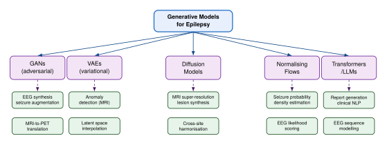
Five families of generative models dominate the epilepsy literature. Figure 2 provides an overview of these families and the clinical tasks they address.
Generative Adversarial Networks (GANs).
GANs (Goodfellow et al., 2014) pit a generator against a discriminator in a minimax game: (GAN Objective) In epilepsy, GANs have been used to synthesise realistic ictal EEG segments (Hartmann et al., 2018; Zhang et al., 2020), to perform unpaired MRI-to-PET translation, and to generate population-diverse training data for multi-site harmonisation.
Variational Autoencoders (VAEs).
VAEs (Kingma & Welling, 2013) learn a stochastic encoder and a generative decoder , optimising the evidence lower bound: (ELBO) In epilepsy, VAEs are valuable for anomaly detection: a model trained on normal-anatomy MRI assigns high reconstruction error to lesional cortex, providing an unsupervised lesion score. VAEs also enable latent-space arithmetic - interpolating between ictal and interictal EEG states, or between pre- and post-surgical MRI.
Diffusion Models.
Diffusion models (Ho et al., 2020; Song et al., 2021) define a forward process that gradually corrupts data with Gaussian noise, and learn a reverse denoising process: (DDPM Reverse) Diffusion models excel at high-fidelity image synthesis and have been applied to MRI super-resolution (recovering 7T-quality texture from 3T acquisitions), lesion synthesis (injecting realistic FCD lesions into normal MRI for training data augmentation), and cross-site harmonisation.
Normalising Flows.
Normalising flows (Rezende & Mohamed, 2015; Papamakarios et al., 2021) learn an invertible mapping with tractable Jacobian, enabling exact likelihood evaluation: (FLOW Likelihood) The tractable likelihood makes flows attractive for seizure forecasting: learning the density of EEG feature trajectories and scoring future windows by their likelihood under the learned model. Low-likelihood windows signal departure from the patient's normal EEG regime - a potential pre-ictal biomarker.
Transformers and Large Language Models.
Autoregressive transformer models treat multi-channel EEG as a sequence of discrete tokens (after vector quantisation) or as continuous patch embeddings, learning long-range temporal dependencies across minutes of recording. Large pre-trained EEG foundation models (e.g., LaBraM, Jiang et al., 2024; BIOT, Yang et al., 2024) are emerging, analogous to BERT and GPT in natural language processing. For clinical text, LLMs summarise EEG reports, extract structured information from clinical notes, and generate draft discharge summaries for epilepsy monitoring unit admissions.
Comparison of Generative Approaches
Table 2 provides a structured comparison of the five families along dimensions most relevant to epilepsy applications.
| Family | Tractable | Sample quality | Training stability | Conditioning | Primary epilepsy use |
| GAN | No | High | Low | Moderate | EEG synthesis, image-to-image |
| VAE | Approx. | Moderate | High | Easy | Anomaly detection, interpolation |
| Diffusion | No (approx.) | Very high | High | Easy | MRI augmentation, harmonisation |
| Flow | Yes | Moderate | Moderate | Moderate | Likelihood scoring, forecasting |
| Transformer | Yes | High (text/seq.) | High | Easy | EEG modelling, report generation |
No single family dominates across all epilepsy tasks. Diffusion models produce the highest-fidelity MRI synthesis but are slow to sample and do not provide tractable likelihoods. Normalising flows provide exact likelihoods but scale poorly to high-dimensional image data without architectural compromises. GANs generate sharp EEG but are prone to mode collapse, which is particularly dangerous in a clinical context because a model that ignores certain seizure morphologies will lead to undertrained detectors. VAEs are the most stable to train and most flexible for anomaly scoring, but their sample quality is limited by the Gaussian decoder assumption. Transformers offer the best solution for sequential EEG modelling at scale.
In practice, the most successful systems combine multiple families. For example, a diffusion model generates synthetic MRI lesions, which augment the training set of a discriminative U-Net segmentor; a VAE encodes patient-specific EEG representations that are then passed to a transformer for seizure forecasting. The chapter will return to these hybrid architectures throughout.
Chapter Roadmap
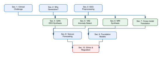
The remainder of this chapter is organised as follows, with a dependency structure illustrated in Figure 3.
- Sec.,3
EEG Signal Characteristics and Preprocessing. Formal description of multi-channel EEG as a multivariate stochastic process; spectral features, time-frequency representations, and graph-theoretic connectivity measures; the preprocessing pipeline from raw recordings to model-ready tensors.
- Sec.,4
GAN-Based EEG Synthesis. Progressive and conditional GAN architectures for ictal EEG generation; evaluation metrics (FID on EEG spectrograms, expert rater studies); downstream seizure detection experiments demonstrating synthetic augmentation benefit.
- Sec.,5
Variational Models for EEG Anomaly Detection. VAE and -VAE for interictal discharge modelling; spike detection via reconstruction error; disentangled latent spaces for seizure type characterisation.
- Sec.,6
MRI Synthesis and Lesion Augmentation. Diffusion models for 3D T1/FLAIR generation; inpainting-based lesion injection for FCD data augmentation; normalising flow-based anomaly scoring for MRI-negative lesion detection.
- Sec.,7
Cross-Modal Translation. Unpaired MRI-to-PET translation with CycleGAN; diffusion-based paired translation; EEG-to-fMRI inference; evaluation of clinical utility for patients missing one modality.
- Sec.,8
Seizure Forecasting with Generative Models. Conditional diffusion and flow-based models for pre-ictal state generation; uncertainty-aware forecasting; evaluation on long-term ambulatory recordings.
- Sec.,9
Foundation Models and Transformers for EEG. Pre-trained EEG transformers; masked autoencoding for EEG; few-shot adaptation to new patients; clinical language models for epilepsy report generation.
- Sec.,10
Ethical and Regulatory Dimensions. Fairness and representativeness of synthetic data; regulatory pathways for AI-generated surgical guidance; explainability and clinician trust; privacy-preserving federated learning with generative augmentation.
Exercises
Exercise 1 (The cost of class imbalance).
A seizure detector is trained on an EEG dataset in which 0.5% of one-second windows contain a seizure (positive class) and 99.5% are seizure-free (negative class).
A naive classifier that always predicts “no seizure” achieves what accuracy? Why does this accuracy not reflect clinical utility?
Define sensitivity (recall) and specificity for this binary classification problem. If a hospital requires a minimum sensitivity of 90%, what is the maximum number of false positives per hour (assuming the alarm is raised for each positive-predicted window) in a 24-hour recording at 256 Hz with non-overlapping 1-second windows?
Suppose a GAN is used to synthesise seizure windows until the positive class constitutes 10% of the training set. What assumptions about the GAN must hold for this synthetic augmentation to improve the true positive rate on held-out real seizure data?
Discuss one failure mode of GAN augmentation in this context that would not occur with oversampling (random duplication of minority-class examples).
Exercise 2 (The epileptogenic zone as a probabilistic concept).
Let denote the true epileptogenic zone (a set of cortical voxels) and let denote the estimated zone from modality .
Formalise the pre-surgical localisation problem as Bayesian inference: write down the posterior and identify what each factor represents clinically.
What conditional independence assumption is typically made in practice when combining evidence across modalities? When might this assumption break down?
Suppose a generative model is trained to synthesise in silico PET maps from MRI. How would you incorporate the output of this model into the Bayesian localisation framework, and what additional uncertainty would need to be tracked?
Exercise 3 (Normalising flows for EEG likelihood scoring).
Let denote a multi-channel EEG segment ( channels, time points) and let be an invertible normalising flow with base distribution .
Write the change-of-variables formula for .
Explain why a flow trained on interictal EEG segments will assign lower log-likelihood to ictal segments, assuming the model has been trained to convergence. What property of a well-trained flow guarantees this?
Propose a threshold-based seizure detection rule using . Define the threshold in terms of a target false-positive rate on a held-out normal recording, and describe how you would set this threshold in a patient-specific versus patient-agnostic manner.
What architectural constraints must satisfy to (i) be invertible and (ii) have a computationally tractable Jacobian determinant? Name one concrete flow architecture that satisfies these constraints for two-dimensional (spatial) data.
Exercise 4 (Generative cross-modal synthesis: a thought experiment).
A hospital has 400 patients with both MRI and FDG-PET, and a further 600 patients with MRI only. A neurologist wants to use PET hypometabolism as a localising biomarker for all 1000 patients.
Describe how an unpaired image-to-image translation model (e.g., CycleGAN) could be trained on the 400 paired patients to synthesise PET from MRI, and then applied to the 600 MRI-only patients. What loss terms does CycleGAN minimise, and what property do they encourage?
Identify two clinical risks of using synthesised PET images for surgical planning without disclosing their synthetic origin to the treating team.
Propose an evaluation protocol to assess whether the synthesised PET maps correctly reflect the location of hypometabolism in the paired validation set (the 400 patients with real PET). Specify at least two quantitative metrics.
The hospital ethics board asks: “Is a synthesised PET scan the same as a real PET scan for regulatory purposes?” How would you answer? What labelling or disclosure requirements would you recommend?
EEG Fundamentals for the Generative Modeller
Before a generative model can be designed, trained, or evaluated on brain-electrical data, its architect must understand the signal. Electroencephalography is deceptively straightforward to record and fiendishly difficult to model: it is simultaneously a rich window into neural dynamics and a superposition of artefacts, volume-conducted fields, and structured noise. This section provides the minimal substrate of EEG knowledge required to make principled decisions about representation, architecture, and evaluation. We approach EEG as mathematicians and engineers, emphasising the properties that constrain and motivate the generative modelling choices taken up in later sections.
What Is EEG? Electrodes, Montages, and the 10–20 System
Electroencephalography measures the time-varying voltage difference between pairs of electrodes placed on the scalp. These voltages reflect the summed post-synaptic potentials of large populations of pyramidal neurons in the cortex, which, when synchronised, produce electrical fields detectable at the scalp surface. A single electrode does not record the activity of a single neuron: the dominant contributors are on the order of to neurons firing more-or-less coherently within a cortical patch, with the field propagated through skull, dura, and scalp via volume conduction.
Definition 4 (EEG Signal).
Let denote the number of active electrodes and the recording length in samples at sampling rate (in Hz). The raw EEG signal is a matrix (Matrix) where entry is the voltage (in microvolts, V) at channel and time sample . Each row is a univariate time series called a channel or electrode trace.
Electrode placement: the 10–20 system.
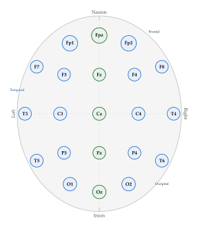
Clinical and research EEG recordings follow the International 10–20 System (standardised by the American Clinical Neurophysiology Society and rooted in work by Jasper, 1958). The name refers to the fact that electrodes are placed at positions that are either 10% or 20% of the distance between two anatomical landmarks: the nasion (bridge of the nose), the inion (posterior protrusion of the skull), and the two pre-auricular points above the ears. This ensures consistent placement across individuals despite differences in head size.
Standard 10–20 recordings use 19 to 21 electrodes for clinical work, while high-density systems extend to 64, 128, or even 256 electrodes. Epilepsy monitoring units typically record at 19–64 channels. Each electrode receives a letter designating the cortical region (F = frontal, C = central, T = temporal, P = parietal, O = occipital, Fp = frontopolar) and a number indicating laterality: odd numbers indicate left-hemisphere placements, even numbers indicate right-hemisphere placements, and the letter z (for “zero”) denotes midline electrodes.
Montages and referencing.
Every EEG voltage is a potential difference and requires a reference. Clinical practice employs several montage conventions. The linked-ears or average reference montage subtracts a global average from each channel, making the signal reference-independent in expectation. The bipolar montage computes differences between adjacent electrode pairs, emphasising local gradients and suppressing global artefacts. The Laplacian montage approximates the second spatial derivative, sharpening spatial resolution. For generative modelling, montage choice affects the covariance structure of : bipolar signals exhibit shorter spatial correlation length than average-referenced signals. Models trained on one montage typically do not transfer to another without re-normalisation.
Formally, a montage is a linear map such that the montaged signal is . For the average reference montage, (the centring matrix). For a bipolar montage, is a sparse difference matrix. Since is fixed and known, data from any montage can be re-montaged to any other, provided the original reference signal is available or reconstructable. This implies that generative models trained on average-referenced data can be used to augment datasets recorded in a bipolar montage by applying the appropriate linear transformation to the synthetic output, a simple but useful domain adaptation strategy.
Sampling rate.
Clinical EEG is recorded at Hz. The Nyquist theorem requires , where is the highest frequency of interest: for epilepsy, high-frequency oscillations (HFOs) at 80–500 Hz have gained diagnostic importance (Jacobs et al., 2012), pushing sampling rates upward. Most large benchmark datasets use Hz or Hz, targeting the clinically canonical 0–100 Hz band. For generative modelling, the choice of determines the temporal dimension of the data matrix and the computational cost of sequence models operating on raw waveforms.
Frequency Bands: The Spectral Vocabulary of EEG
Clinical EEG interpretation is organised around five canonical frequency bands, each associated with distinct neural states and pathological signatures.
Definition 5 (EEG Frequency Bands).
The five canonical EEG frequency bands are:
1.35
Band Range (Hz) Normal association Epilepsy relevance Delta () – Deep sleep, infants Post-ictal slowing, focal lesions Theta () – Drowsiness, memory Pre-ictal build-up, temporal lobe Alpha () – Relaxed wakefulness Attenuated during seizure onset Beta () – Active cognition Ictal fast activity, drug effect Gamma () –+ Sensorimotor binding High-frequency ictal onset, HFOs
Spectral evolution during seizures.
During a generalised tonic-clonic seizure the spectral composition evolves in a stereotyped pattern: the tonic phase begins with high-frequency (beta/gamma, 15–60 Hz) low-amplitude activity, transitions to low-frequency (delta/theta, 1–7 Hz) high-amplitude rhythmic discharges during the clonic phase, and terminates with diffuse delta slowing in the postictal period. Focal onset seizures evolve from a localised fast onset zone to progressively broader delta-dominated propagation. This stereotyped evolution is a constraint that generative models should satisfy: synthetic ictal segments should exhibit frequency chirp (the characteristic shift from high to low frequency over time) rather than static spectral profiles. Evaluating whether a generative model preserves ictal spectral evolution is one of the domain-specific fidelity checks discussed in sec:epilepsy:evaluation.
Each band is not a fixed property of the recording but an interpretation applied by bandpass filtering. In practice a zero-phase fourth-order Butterworth filter or a Morlet wavelet decomposition is applied to isolate each band. The relative power in each band, computed as (Bandpower) where is the power spectral density, constitutes a simple but powerful feature vector for seizure detection. Generative models operating in the frequency domain must respect these band boundaries, as band power ratios encode diagnostically meaningful information that should be preserved or controllably varied during synthesis.
Remark 1 (High-Frequency Oscillations).
HFOs (80–500 Hz) have emerged as a biomarker for epileptogenic tissue. They are subdivided into ripples (80–250 Hz) and fast ripples (250–500 Hz). Detecting and synthesising HFOs requires sampling rates of at least 1000 Hz and architecture choices that do not low-pass the signal. Generative models targeting HFOs represent an active research frontier (Frauscher et al., 2017).
Seizure States: Interictal, Preictal, Ictal, Postictal
From the perspective of a supervised learning system, the EEG time axis can be partitioned into four states relative to a seizure event. Understanding these states is essential for designing labelling schemes, choosing data windows, and interpreting classifier outputs.
Definition 6 (Seizure States).
Let denote the clinical onset of a seizure (as annotated by an epileptologist) and its clinical termination. The four EEG states are:
Interictal (): the period between seizures, typically hours to days. EEG appears near-normal but may contain interictal epileptiform discharges (IEDs) such as spikes, sharp waves, and spike-and-wave complexes, which are pathological but not seizure activity.
Preictal (): the transitional period immediately preceding seizure onset, for some lookahead horizon (typically 5–60 minutes in the prediction literature). EEG changes are subtle, sometimes invisible to the naked eye; their existence is contested for some patients.
Ictal (): the seizure itself, typically seconds to minutes. EEG shows dramatic rhythmic discharges, evolving patterns, and widespread synchronisation. The ictal state is the primary target for seizure detection algorithms.
Postictal (): the recovery period following seizure termination, characterised by diffuse slowing (suppression), increased delta power, and gradual return to baseline. Duration ranges from minutes to hours depending on seizure severity.
Remark 2 (Annotation Granularity).
Clinical annotations mark and , but the preictal window is set by the researcher and varies widely across the literature (from 5 minutes in Moghim & Corne, 2014, to 4 hours in Brinkmann et al., 2016). This choice profoundly affects the class imbalance ratio and the difficulty of the prediction task. A generative model producing synthetic preictal segments must respect the chosen or risk contaminating the preictal class with interictal samples.
Remark 3 (Inter-Rater Variability in Seizure Annotation).
Seizure annotations are not ground truth. Studies of inter-rater agreement among epileptologists on scalp EEG datasets report (Cohen's kappa) values in the range 0.55–0.80 for seizure type and 0.70–0.90 for onset time, where perfect agreement would give . Annotation disagreement means that a generative model trained on one annotator's labels may produce data that a second annotator would classify differently. This limits the theoretical upper bound of classifier performance and complicates the evaluation of synthetic data quality: a synthesised seizure that looks correct to a neurologist but was labelled by a different neurologist than the training set may be rejected by automated quality metrics.
EEG micro-states and within-state heterogeneity.
Even within the interictal state, EEG is not homogeneous. EEG micro-states (Lehmann et al., 1998) are quasi-stable scalp topography patterns lasting 80–120 ms, transitioning semi-randomly in a Markov-like sequence. Four canonical micro-state templates (labelled A, B, C, D) have been identified across subjects, with their transition probabilities altered in epilepsy and other neurological conditions. Within the ictal state, seizures undergo a structured evolution through multiple electrographic patterns (electrographic seizure phases): the pre-discharge build-up, fast low-voltage onset, organised rhythmic discharge, clonic phase, and termination. A generative model that collapses all ictal windows into a single distribution fails to capture this within-class heterogeneity, producing homogeneous synthetic data that does not replicate the temporal evolution characteristic of real seizures.
Signal Characteristics: Non-Stationarity, High Dimensionality, and Noise
Three properties of EEG are particularly consequential for generative modelling.
Non-stationarity.
A stochastic process is (weakly) stationary if its mean and autocovariance function do not change with time. EEG violates both conditions over timescales beyond a few seconds: mean amplitude drifts with electrode impedance and posture; spectral content changes with vigilance state, drug effect, and disease progression; seizures introduce abrupt statistical shifts. More formally, if denotes a window of length seconds, the covariance matrix is not constant in .
This non-stationarity constrains generative modelling in two ways. First, models that assume stationarity (e.g., stationary Gaussian process priors) will fail to capture the ictal transition. Second, evaluation metrics computed on long recordings may average away the very phenomena of interest. Practitioners address non-stationarity by operating on short windows (typically 1–30 s) and treating windows as i.i.d. samples, though this approximation ignores temporal dependencies between windows.
Insight.
An important design decision for generative EEG models is whether to operate on raw waveforms, spectral representations, or spatial covariance matrices. Raw waveforms preserve all information but require architectures with long effective receptive fields (e.g., temporal convolutional networks, transformers). Spectral representations discard phase but reduce the sequence length by a factor proportional to the hop size, enabling standard image generative architectures. Spatial covariance matrices (symmetric positive definite matrices) capture inter-channel dependencies but discard temporal dynamics. Each representation encodes a different facet of neural activity, and no single representation is universally optimal for generative modelling: the best choice depends on the downstream task.
A more principled approach is to model EEG as a locally stationary process: one whose second-order statistics change slowly relative to the timescale of a short analysis window. Let be the instantaneous multichannel EEG vector. The locally stationary covariance model posits (Locally Stationary) which is adequate for window lengths small relative to the seizure timescale. VAEs and diffusion models operating on short windows implicitly adopt this approximation by treating each window as a sample from a fixed latent distribution. Recurrent generative architectures can relax this assumption by conditioning on the previous window's latent state.
High dimensionality.
With channels sampled at Hz for seconds, the raw data matrix has elements. At 64 channels, 512 Hz, and 10 hours of recording: (Dimensionality) Fitting a generative model directly on raw multi-channel waveforms of this size is computationally prohibitive without compression. The standard pipeline first projects the data into a lower-dimensional representation (spectral features, ICA components, or learned latent codes) before applying the generative model.
Two classical linear dimensionality reduction techniques are frequently applied as preprocessing for EEG generative models:
Independent Component Analysis (ICA). ICA factorises the observed -dimensional signal into statistically independent components: , where is the mixing matrix and contains the independent source signals. Artefact components (eye blinks, muscle) are identified by their non-neural topographic maps and removed before reconstruction. ICA reduces effective dimensionality because artefact-cleaned recordings typically have rank lower than .
Common Spatial Patterns (CSP). CSP computes spatial filters that maximise the variance ratio between two classes. For the binary ictal/non-ictal problem, CSP finds () such that is maximised. The projected signal is a compact representation that concentrates ictal information in a small number of components. CSP is widely used as a preprocessing step before VAE or GAN training, reducing input dimension from to components while retaining most of the discriminative structure.
Noise and artefacts.
EEG recordings are corrupted by several artefact sources, each with a distinct spectral and spatial signature:
Muscle artefacts (EMG): broadband high-frequency contamination (20–200 Hz), prominent at temporal and frontal electrodes near jaw and neck muscles.
Eye movement artefacts (EOG): large-amplitude deflections at frontopolar electrodes (Fp1, Fp2) from cornea rotation; blinks produce stereotyped biphasic waveforms.
Cardiac artefacts (ECG): regular 1–1.5 Hz pulses, visible at temporal and frontal electrodes.
Line noise: 50 Hz (Europe, Asia) or 60 Hz (Americas) sinusoidal contamination from AC power.
Movement artefacts: irregular baseline shifts from electrode cable movement.
A generative model trained without artefact removal may learn to synthesise artefacts as if they were neural signals, producing data that appears realistic to automated metrics but is clinically misleading.
Time-Frequency Representations
Because EEG is non-stationary, the global power spectrum discards temporal information. The solution is a time-frequency representation (TFR) that tracks how spectral content evolves over time.
Definition 7 (Short-Time Fourier Transform).
Let be a single EEG channel. The short-time Fourier transform (STFT) with window function of length and hop size is (STFT) for frame index and frequency bin . The spectrogram is the squared magnitude , a real-valued matrix that can be treated as an image by convolutional generative architectures.
Definition 8 (Continuous Wavelet Transform).
The continuous wavelet transform (CWT) with mother wavelet is (CWT) where is the scale parameter (inversely related to frequency) and is the translation (time) parameter. For epilepsy analysis, the Morlet wavelet is the standard choice, offering Gaussian localisation in both time and frequency.
The TFR (or ) has two key advantages for generative modelling: (i) it converts the 1-D time series into a 2-D image, enabling architectures designed for image synthesis (GANs, VAEs, diffusion models) to operate without modification; (ii) it separates seizure-relevant spectral changes (e.g., ictal onset manifests as a sudden power increase in the beta or gamma band) from slow baseline drifts. The primary cost is the loss of phase information (in the spectrogram) and the Heisenberg uncertainty trade-off: improving temporal resolution degrades frequency resolution, and vice versa.
Definition 9 (Time-Frequency Uncertainty Principle).
For any window function with time spread and frequency spread (defined as the standard deviations of and respectively): (Uncertainty) The Gaussian window (Morlet wavelet) achieves equality, making it the optimal window for simultaneous time and frequency localisation. For seizure analysis, the practical implication is a trade-off: a 1-second STFT window resolves spectral bands to Hz but cannot localise seizure onset to better than s; a 64-ms window localises onset to ms but smears spectral structure across Hz.
Mel-frequency spectrograms for EEG.
Mel-frequency spectrograms, standard in audio generative modelling, have been adapted for EEG synthesis. The mel scale compresses frequency resolution at high frequencies according to , which is physiologically motivated for speech but has no direct neurophysiological justification for EEG. Nevertheless, several papers report that GANs conditioned on mel spectrograms produce higher-quality EEG than those conditioned on linear spectrograms, possibly because the lower-dimensional mel representation regularises the generator and prevents mode collapse onto artefactual high-frequency patterns.
Phase-sensitive representations.
The spectrogram discards phase, which encodes neural synchrony and connectivity information of diagnostic relevance (e.g., phase synchrony between bilateral temporal electrodes is altered during focal seizures). Phase-preserving alternatives include:
Complex spectrogram: retain both and as separate image channels. This doubles the representation dimension but allows the generative model to learn phase structure.
Phase coherence matrix: compute the instantaneous phase at each channel via the Hilbert transform and encode inter-channel phase synchrony as a matrix with ; this is the phase locking value between channels and .
Raw waveform: bypass time-frequency transformation entirely and operate the generative model on the raw 1-D signal. Architectures such as WaveNet (van den Oord et al., 2016) and autoregressive transformers can operate at the sample level, preserving all phase information, at the cost of much longer sequence lengths.
Example 2 (Reading an EEG Spectrogram for Seizure Onset).
Consider a single 60-second EEG epoch recorded at Hz from electrode T3 in a patient with right temporal-lobe epilepsy. A Morlet CWT with 40 logarithmically spaced scales covering 1–60 Hz produces a scalogram.
Interictal baseline (0–30 s): The scalogram shows high-amplitude alpha power (8–13 Hz) during wakefulness, with intermittent theta spikes coinciding with annotated interictal discharges. Background power is roughly : lower-frequency bands dominate in absolute power.
Preictal transition (30–40 s): A subtle but detectable increase in theta/alpha power (– Hz) appears approximately 7 seconds before the clinician-marked onset. The normalised log-power ratio rises by dB - detectable algorithmically but indiscernible to the naked eye on the raw trace.
Ictal onset (40 s): A sharp, rhythmic discharge at Hz initiates in the theta band. Over the following 5–10 seconds the discharge evolves: frequency increases toward 10 Hz (alpha), amplitude grows, and the pattern recruits adjacent channels. In the scalogram this appears as a bright horizontal streak that shifts upward in frequency over time-a hallmark of temporal-lobe seizures.
Post-ictal (50–60 s): Following termination, the scalogram shows abrupt suppression of all frequencies above 4 Hz (delta slowing), then gradual spectral recovery.
A generative model conditioned on seizure state labels must learn to reproduce these four distinct scalogram textures and, crucially, the transition dynamics between them. Failure to model the transition produces a distribution mismatch that downstream classifiers may exploit as a tell.
Key Benchmark Datasets
The epilepsy EEG community has converged on a small number of public benchmark datasets. Understanding their provenance, size, and limitations is essential for reproducible evaluation of generative models.
| Dataset | (Hz) | Approx. IR | Key features | ||
| CHB-MIT Scalp EEG | 23 | 198 | 256 | 50:1 | Paediatric, long-term, public |
| TUH EEG Corpus | 14,987 | 14,000 | 250–512 | 200:1 | Largest public corpus, clinical |
| EPILEPSIAE | 30 | 275 | 512–2048 | 130:1 | Multi-centre, intracranial option |
| Siena Scalp EEG | 14 | 47 | 512 | 80:1 | Adult, PhysioNet hosted |
| Kaggle Melbourne (2014) | 10 | varies | 400 | 50:1 | Intracranial (dogs + humans) |
CHB-MIT Scalp EEG Database.
The CHB-MIT database (Shoeb, 2009; maintained at PhysioNet) comprises scalp EEG recordings from 23 paediatric patients (ages 1.5–22 years) with intractable seizures, recorded at Boston Children's Hospital using the international 10–20 system at 256 Hz. Total recording length exceeds 980 hours, containing 198 annotated seizures. It is the most widely cited benchmark for seizure prediction and detection, despite its relatively small patient cohort, because of its accessibility, documentation quality, and community familiarity.
Temple University Hospital (TUH) EEG Corpus.
The TUH EEG Corpus (Obeid & Picone, 2016) is the largest public EEG repository, compiled from clinical recordings at Temple University Hospital spanning 2002–present. The Seizure Corpus (TUSZ) release v1.5.2 contains recordings from over 675 subjects with more than 5700 seizure annotations across four seizure types (focal, generalised, combined, and unknown). The corpus is clinically representative but heterogeneous: recordings vary in channel count (19–32), sampling rate (250–512 Hz), and clinical quality, demanding robust normalisation pipelines.
EPILEPSIAE.
EPILEPSIAE (Ihle et al., 2012) is a European multi-centre dataset containing long-term EEG recordings from 30 patients with pharmacologically intractable focal epilepsies. Each patient contributes at least 24 hours of continuous EEG, and many contribute several days. The dataset is particularly valuable for seizure prediction (as opposed to detection) because of the long preictal windows available. Access requires signing a data-use agreement.
Siena Scalp EEG Database.
The Siena dataset (Detti et al., 2020), hosted on PhysioNet, provides scalp EEG recordings from 14 adult subjects at 512 Hz. It is notable for including precise onset/offset annotations and is frequently used as a held-out test set for models trained on CHB-MIT.
Kaggle American Epilepsy Society Seizure Prediction Challenge (2014).
This competition dataset contains intracranial EEG recordings from four dogs and three humans, sampled at 400 Hz with 16 electrodes. While smaller than the scalp datasets, it offers intracranial resolution and was influential in spurring deep learning approaches to seizure prediction (Brinkmann et al., 2016).
Emerging datasets and data federation.
Two emerging trends will affect the next generation of generative EEG models. First, federated datasets: privacy-preserving frameworks (e.g., TEFLA, IBIS) allow multiple hospitals to train shared models without transferring raw patient data, addressing the legal constraints that have limited the size of public EEG repositories. Second, wearable EEG: consumer-grade EEG headbands (Emotiv, Muse, OpenBCI) are producing large real-world datasets outside clinical settings, with fewer electrodes (2–14 channels) but far more continuous recording time. Generative models trained on clinical 19-channel datasets will face significant domain shift when applied to wearable 2-channel recordings, motivating domain adaptation techniques discussed in later sections.
Remark 4 (Dataset Fragmentation and Reproducibility).
The field suffers from a reproducibility crisis partly attributable to inconsistent preprocessing pipelines applied to the same datasets. Studies using CHB-MIT, for example, vary in their choice of montage, bandpass filter bounds, window length, seizure-free minimum gap, and cross-validation scheme, making direct comparison of published numbers unreliable. Generative augmentation papers inherit this fragmentation: a model that improves AUC on one preprocessing of CHB-MIT may show no improvement on another. Standardised preprocessing pipelines (such as those provided by the MNE-Python library) are strongly recommended.
Cross-Dataset Generalisation and Domain Shift
A generative model trained on CHB-MIT will not, in general, produce valid EEG for a TUH Corpus patient. The two datasets differ along multiple axes that together constitute domain shift:
Patient population: CHB-MIT covers paediatric patients with a narrow age range; TUH Corpus covers the full adult clinical spectrum. Brain electrical patterns change substantially with age, with children exhibiting higher amplitude, lower frequency baseline rhythms.
Recording hardware: different amplifier manufacturers impose different frequency responses, quantisation levels, and impedance tolerances.
Clinical protocol: medication changes, sleep staging, and the clinical reason for the recording (monitoring vs. diagnostic) affect the EEG non-stationarity and artefact profile.
Seizure aetiology: temporal-lobe seizures (dominant in CHB-MIT) have different ictal morphologies than frontal-lobe or generalised seizures.
Domain shift is particularly damaging for generative augmentation because the generative model learns the source domain distribution ; samples from this model contaminate the target domain training set with out-of-distribution data. Techniques for domain-adaptive generative augmentation, including conditional normalising flows conditioned on patient identifiers and adversarial domain adaptation losses, are discussed in sec:epilepsy:advanced.
Historical Note.
From analogue paper charts to deep networks. The electroencephalogram was first recorded in humans by Hans Berger in 1924, published in 1929. For fifty years, EEG interpretation was entirely visual: a clinical neurophysiologist read paper charts produced by ink-and-paper galvanometers, identifying abnormalities from waveform morphology. The first automated seizure detectors appeared in the 1970s, using threshold-crossing rules on analogue signals (Ives et al., 1974). Digital EEG arrived in clinical practice in the late 1980s, enabling computer-assisted analysis. Early machine learning approaches (Fisher, 1994; Osorio et al., 1998) used hand-engineered features fed to support vector machines and linear discriminants. The deep learning revolution reached EEG analysis around 2016 (Acharya et al., 2018), and the first GAN-based EEG synthesis paper (Hartmann et al., 2018) appeared in 2018. The first diffusion model applied to EEG synthesis (Kim et al., 2022) appeared just four years later, illustrating the rapid adaptation of generative modelling techniques to this domain.
The Class Imbalance Problem
No aspect of EEG-based epilepsy machine learning is more persistently disruptive than class imbalance. The neurophysiological reality is stark: a patient who experiences two generalised tonic-clonic seizures per week, each lasting two minutes, generates approximately of their interictal EEG as ictal data. The other is “normal”. A classifier that labels every window as non-seizure achieves accuracy while being useless. Addressing this imbalance is not optional: it is the central engineering problem of the field.
Quantifying the Imbalance
Definition 10 (Class Imbalance Ratio).
Let and denote the number of training windows belonging to the minority (seizure) and majority (non-seizure) classes, respectively. The imbalance ratio (IR) is (IR) For most long-term EEG datasets, . Using 4-second non-overlapping windows at 256 Hz, a typical CHB-MIT patient contributes – ictal windows against – interictal windows.
The imbalance is compounded by the temporal clustering of both classes: seizures arrive in clusters separated by long seizure-free periods, and the interictal class is itself heterogeneous (drowsiness, drug troughs, artefacts). A model that memorises a few ictal patterns will generalise poorly across a patient's full seizure repertoire.
Remark 5 (Temporal Proximity Bias).
A subtle form of bias arises when training and test windows are drawn from the same recording session without enforcing a temporal gap. Because EEG dynamics evolve slowly, windows that are close in time tend to be more similar than distant windows, even across the train-test split. A classifier trained on windows immediately before a test seizure will see data that is very similar to the test preictal window, inflating apparent performance. This is sometimes called temporal leakage. The standard remedy is to define train and test sets by seizure event rather than by window: the last seizures of each patient constitute the test set, and all remaining seizures (with surrounding context) form the training set. Generative augmentation must respect this split: the generative model must be trained exclusively on training-set windows and its outputs added only to the training set.
Patient-level heterogeneity.
Imbalance ratios vary enormously across patients in the same dataset. In CHB-MIT, patient chb24 has an IR of approximately 9 (relatively balanced) while patient chb12 has an IR exceeding 400. Pooling patients without stratification produces a combined dataset that is dominated by patients with high IR, systematically underrepresenting easy cases and overfitting to the seizure morphology of high-seizure patients.
Why Standard Machine Learning Fails on Imbalanced EEG
A standard empirical risk minimiser minimises the average loss over the training set. When , the empirical risk is dominated by the majority class, and the optimal decision boundary is pushed toward (or coincides with) the boundary of the minority class manifold.
Proposition 1 (Bias of the Naive Classifier).
Let denote the minority class proportion. A classifier minimising cross-entropy loss will converge to the trivial predictor that outputs (non-seizure) whenever the minority class loss gradient is smaller than the majority class loss gradient in expectation. Specifically, if and , the gradient contribution of the minority class is scaled by : (Gradient Imbalance) When , the second term dominates and the model learns primarily to classify non-seizure windows.
The practical consequences are severe:
High specificity, catastrophically low sensitivity. Models trained naively achieve specificity (correctly rejecting non-seizure) but sensitivity (correctly identifying seizure), often below chance for rare patients.
Overconfident majority predictions. Calibration is poor: the model assigns high confidence to almost all inputs, preventing threshold tuning from recovering minority class performance.
Poor feature learning for the minority class. When minority samples are rare, the network's internal representations for the minority class are learnt from too few examples and tend to cluster tightly around a small number of prototypical patterns observed in training, failing to cover the full ictal manifold.
Traditional Solutions and Their Limitations
The machine learning literature offers three classical families of remedies for class imbalance: data-level methods, algorithm-level methods, and hybrid methods.
Data-level methods: oversampling and undersampling.
The simplest approach is random oversampling: replicate minority class windows until the classes are balanced. This introduces no new information and tends to cause overfitting, since the classifier sees identical minority examples many times. Random undersampling discards majority class windows, wasting labelled data.
SMOTE (Synthetic Minority Over-sampling Technique; Chawla et al., 2002) improves on random oversampling by synthesising new minority samples as convex combinations of existing minority samples and their -nearest neighbours: (Smote) where is a nearest neighbour of in the feature space.
ADASYN (Adaptive Synthetic Sampling; He et al., 2008) extends SMOTE by generating more synthetic samples in feature-space regions where the classifier boundary is most uncertain, weighted by the local class density.
Limitations of interpolation-based methods.
Both SMOTE and ADASYN assume that the minority class manifold is convex: that any convex combination of two minority samples is a valid minority sample. For EEG signals, this assumption fails in at least three ways:
Non-Euclidean feature geometry. Seizure waveforms live on a nonlinear manifold in raw sample space. Linear interpolation between two ictal windows may produce signal combinations that are neither ictal nor interictal, but physiologically impossible.
Temporal structure violation. EEG windows have strong temporal autocorrelation. SMOTE operates on window-level feature vectors, ignoring the within-window waveform structure. Interpolating between two windows discards the autocorrelation structure, producing flat or artifactual power spectra.
Diversity collapse. When is very small (e.g., ), the SMOTE graph has few edges and the synthetic distribution is limited to a low-dimensional convex hull of the observed ictal samples. If those samples share a common seizure morphology, the augmented set fails to cover the full ictal manifold.
Algorithm-level methods: class weighting and cost-sensitive learning.
Rather than modifying the data, algorithm-level methods modify the loss function. Class weighting multiplies the loss for minority class samples by a weight , typically with : (Weighted LOSS) This counteracts the gradient imbalance in (Gradient Imbalance) but does not increase the diversity of minority class patterns seen by the model. Focal loss (Lin et al., 2017) reduces the weight of well-classified majority examples dynamically: , where down-weights easy negatives.
Hybrid methods: ensemble approaches.
Balanced bagging (Maclin & Opitz, 1997) combines undersampling with ensemble learning: each base classifier is trained on a balanced bootstrap sample obtained by taking all minority class samples and a random subsample of majority class samples of equal size. Because each bootstrap uses a different majority subsample, the ensemble collectively exploits more of the majority class data while each individual classifier is not overwhelmed by the majority. For EEG, balanced random forests (a variant of balanced bagging applied to decision trees) were a competitive baseline before deep learning. Their limitation is the same as all undersampling methods: they waste majority class information and cannot enrich the minority class distribution.
Summary of limitations.
None of the classical approaches addresses the root problem: the model has too little information about the minority class manifold. Class weighting and focal loss rearrange the training signal without adding information. SMOTE and ADASYN add synthetic information but assume a convex manifold that does not hold for physiological waveforms. Ensemble methods exploit available majority data better but still cannot generate novel minority patterns. The natural next step is to learn the minority class manifold from data using a generative model, which we take up in the following sections.
Generative Augmentation: Learning the Data Manifold
Key Idea.
Manifold-Aware Augmentation. Classical augmentation methods (SMOTE, ADASYN, random oversampling) operate by interpolating in feature space, implicitly assuming that the minority class manifold is convex. Generative models instead learn a probability distribution supported on the minority class manifold from the available training examples. New synthetic samples are drawn by sampling from , not by interpolating between existing examples. This distinction has three practical consequences:
Samples from can explore the full support of the minority distribution, including regions between and beyond the training examples, provided the model generalises.
The generative model can be conditioned on clinical covariates (patient identity, seizure type, recording conditions), enabling targeted augmentation in the directions of highest decision boundary uncertainty.
Unlike SMOTE, which operates on any feature vector, generative models produce coherent waveforms that respect the within-sample temporal and spectral structure of EEG, because they are trained to maximise the likelihood of valid EEG sequences.
Comparison of augmentation strategies.
Table 4 summarises the key properties of the main augmentation families for EEG class imbalance.
| Method | Manifold- | |||
| aware | Phase- | |||
| preserving | Small | |||
| Requires | ||||
| training? | ||||
| Random oversampling | No | Yes | Yes | No |
| SMOTE | Partial | No | Limited | No |
| ADASYN | Partial | No | Limited | No |
| Class weighting | No | - | Yes | No |
| Focal loss | No | - | Yes | No |
| VAE augmentation | Yes | Yes | Moderate | Yes |
| GAN augmentation | Yes | Yes | Limited | Yes |
| Diffusion augmentation | Yes | Yes | Yes | Yes |
How much augmentation is enough?
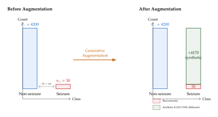
A natural question is how many synthetic samples to generate. Naïvely setting targets perfect balance (IR ), but this may not be optimal. Several empirical studies (Estabrooks et al., 2004, for tabular data; Wang et al., 2018, for EEG) suggest that the optimal augmentation ratio depends on three factors: (i) the quality of the generative model (higher quality supports higher ); (ii) the complexity of the target classifier (deeper classifiers are more prone to memorising low-quality synthetic samples); (iii) the heterogeneity of the true minority distribution (more heterogeneous distributions require more samples to cover). A practical heuristic is to sweep on a validation fold and select by AUPRC.
The practical pipeline for generative augmentation in epilepsy classification is as follows:
Train generative model on available minority class windows . Architectures include conditional GANs, VAEs, and diffusion models, discussed in sec:epilepsy:gans,sec:epilepsy:vae,sec:epilepsy:diffusion.
Generate synthetic minority windows with (or some desired balance ratio) by sampling from .
Augment the training set: .
Train classifier on using standard cross-entropy, without class weighting.
Evaluate on a held-out test set containing real signals only; synthetic data are never used for evaluation.
Evaluation Metrics for Imbalanced Settings
Accuracy is a misleading metric when classes are imbalanced: a model achieving 99% accuracy by predicting only non-seizure provides no clinical value. The epilepsy EEG literature employs a family of metrics that treat the two classes asymmetrically, reflecting the clinical asymmetry of the consequences of false negatives (missed seizures) versus false positives (unnecessary alarms).
Definition 11 (Confusion Matrix for Binary Seizure Detection).
Let be pairs of true and predicted binary labels, with denoting seizure. Define: (Confusion)
Definition 12 (Performance Metrics for Imbalanced EEG).
The primary metrics are: (Sensitivity) where ranges over all possible decision thresholds.
Clinical interpretation.
Sensitivity measures the fraction of actual seizure windows correctly identified. In clinical deployment, a missed seizure (FN) has catastrophic consequences (patient injury, sudden unexpected death in epilepsy – SUDEP), while a false alarm (FP) causes inconvenience but not direct harm. This asymmetry motivates primary optimisation for sensitivity at a fixed tolerable FPR. Clinical seizure detection systems typically target sensitivity at FPR false alarms per hour.
AUROC and AUPRC.
AUROC is threshold-independent and robust to class imbalance in the sense that it measures the probability that a randomly drawn positive example is scored higher than a randomly drawn negative example. However, for very high IR, the Precision-Recall curve and its area (AUPRC) are more informative, as AUROC can remain high even when precision is near zero. Davis & Goadrich (2006) establish that AUPRC is the appropriate metric when IR and high precision is required.
False alarms per hour.
In ambulatory and wearable seizure detection, sensitivity and specificity are often replaced by a two-dimensional operating point: sensitivity (fraction of seizures detected) plotted against the false alarm rate measured in alarms per hour (FAR). This metric is clinically intuitive: a device that triggers 10 alarms per hour is clinically useless regardless of its sensitivity. Clinical targets are typically FAR alarm/hour at sensitivity . Receiver Operating Characteristic (ROC) curves parameterised by FAR rather than FPR are sometimes called DETA (Detection Error Trade-off Analysis) curves in the seizure literature.
Event-based vs. window-based metrics.
A subtle but important distinction separates window-based from event-based evaluation. Window-based evaluation treats each time window as an independent sample; event-based evaluation assesses whether the classifier correctly detects each seizure event (onset to offset) with at most seconds of latency. A model can achieve high window-level sensitivity by firing on many windows within a single seizure, while still missing an entire seizure event at another time. International conference competitions (e.g., EPILEPSIAE, Kaggle) have moved toward event-based scoring, and generative augmentation papers should report both.
Seizure prediction-specific metrics.
Seizure prediction (forecasting a seizure before it occurs) introduces additional metric complexity. A prediction issued in the preictal window of width is counted as true positive; a prediction outside the preictal window is a false positive. The time in warning (TIW) metric measures the fraction of time spent in the alarm state, a measure of disruption to patient quality of life. An ideal predictor has high sensitivity, low FPR, and low TIW. The Poisson process benchmark provides a natural baseline: a random predictor that issues alarms at rate achieves expected sensitivity and TIW per hour. Any learned predictor should beat this Poisson baseline to be considered non-trivial (Mormann et al., 2006).
Practical Considerations for Imbalanced EEG Pipelines
Stratified cross-validation.
Naive -fold cross-validation over windows can allocate all minority windows to the same fold, creating folds with zero positive examples. Stratified -fold cross-validation ensures that each fold contains approximately positive windows. For EEG, stratification should be applied at the seizure event level, not the window level, to avoid temporal leakage.
Normalisation and whitening.
Before training either the generative model or the downstream classifier, EEG windows must be normalised. Common choices are:
Global z-score: subtract the mean and divide by the standard deviation computed over the training set.
Per-channel z-score: normalise each channel independently to zero mean and unit variance over the training set. This removes amplitude differences between channels while preserving relative channel-to-channel power differences.
Robust normalisation: subtract the median and divide by the interquartile range; robust to outliers caused by artefact windows.
Normalisation parameters (mean, standard deviation) must be computed on the training fold only and applied without re-fitting to the validation and test folds. Generative models must synthesise data in the normalised space; if the model operates in the raw amplitude space, the synthetic windows must be normalised before being added to the augmented training set.
Validation strategy for generative augmentation.
Evaluating generative augmentation requires a three-way split: (i) a training set on which both the generative model and the downstream classifier are trained; (ii) a validation set used for hyperparameter selection (augmentation ratio, generative model architecture); (iii) a test set reserved for final evaluation. A common mistake is to use the validation set performance to choose the augmentation ratio, then report test set performance as if it were unbiased. Proper practice requires that the test set is touched exactly once, after all hyperparameters have been frozen.
Remark 6 (Evaluation Contamination).
A critical error in the generative augmentation literature is including synthetic samples in the test set. Evaluation must be performed on real test windows only; synthetic samples serve exclusively as training-time augmentation. Several published papers violate this principle, reporting artificially inflated metrics. Reviewers should verify that the test fold consists exclusively of held-out real data, with no temporal overlap with the training fold (i.e., the last seizures, not a random -fold split which may leak preictal context).
Section Summary
Class imbalance is the central data challenge of EEG-based epilepsy machine learning. The key facts established in this section are:
Seizure windows constitute 0.01–2% of total recording time in typical long-term EEG datasets, yielding imbalance ratios of 50:1 to 500:1.
Standard empirical risk minimisers converge to majority-class predictors when , because the minority class contributes fraction of the gradient in expectation.
Classical remedies (SMOTE, ADASYN, class weighting) address the symptom (imbalance) without addressing the root cause (too little information about the minority manifold).
Generative augmentation learns a probability distribution supported on the minority class manifold, producing diverse synthetic samples that respect the temporal, spectral, and spatial structure of real ictal EEG.
Evaluation must use imbalance-robust metrics (sensitivity, AUPRC, event-based detection rate at fixed FAR) and must never include synthetic samples in the test fold.
The remainder of this chapter develops the specific generative architectures (GANs in sec:epilepsy:gans, VAEs in VAEs and Hybrid Generative Models, diffusion models in sec:epilepsy:diffusion) and their application to seizure augmentation, cross-patient transfer, and seizure simulation.
Exercise 5.
A 2-second EEG window is recorded at Hz from electrode C3. The window is passed through a 512-point FFT (zero-padded).
- (a)
What is the frequency resolution of the FFT output? How many FFT bins fall within the alpha band (8–13 Hz)?
- (b)
Compute the band power for the alpha band by summing the squared magnitudes of the relevant FFT bins and normalising by the total power. Write the formula explicitly.
- (c)
During a seizure, the alpha band power drops by 80% and the beta band power increases by 200% relative to the interictal baseline. If the interictal alpha-to-beta power ratio is 2.5, compute the ictal alpha-to-beta ratio.
- (d)
Explain why a generative model that produces synthetic ictal windows with the correct total power but incorrect band power ratios may be detected as synthetic by a frequency-aware discriminator.
Exercise 6.
A long-term EEG recording contains 72 hours of data at 256 Hz, recorded with 19 channels using 10-second non-overlapping windows. The recording contains 8 seizures with an average duration of 90 seconds each.
- (a)
Compute the total number of non-overlapping windows .
- (b)
Compute (ictal windows) and (non-ictal windows), assuming every window whose centre falls within a clinician-annotated seizure is labelled as ictal.
- (c)
Compute the imbalance ratio .
- (d)
If SMOTE is applied with nearest neighbours to balance the classes, how many synthetic windows are generated? What is the total training set size after SMOTE?
Exercise 7.
Let the feature space be with (representing 256 Hz 2 seconds per window, flattened). Suppose ictal windows are available.
- (a)
Compute the maximum number of distinct edges in the SMOTE -nearest-neighbour graph (with ).
- (b)
Argue that the SMOTE synthetic distribution is supported on a union of at most line segments in . What fraction of the unit ball in does this support occupy?
- (c)
Explain qualitatively why the answer to (b) motivates learning a full generative model over the minority class manifold instead of interpolating.
Exercise 8.
Consider a binary seizure classifier applied to a dataset with ictal and non-ictal windows. The classifier outputs a score , and at threshold achieves TP , FP , FN , TN .
- (a)
Compute sensitivity, specificity, FPR, precision, F, and accuracy.
- (b)
Show that accuracy is misleading as a performance metric by computing the accuracy of the trivial classifier .
- (c)
A competitor reports “our model improves AUROC from 0.91 to 0.94 with generative augmentation.” Explain why this might not correspond to a clinically meaningful improvement. What alternative metric would you prioritise, and why?
- (d)
Suppose the generative augmentation paper computes AUPRC on a test set that includes 500 synthetic ictal windows. Explain the error and its expected direction of bias.
Exercise 9.
The focal loss for binary classification is , where if and if , and is the class-dependent weighting factor.
- (a)
Show that when and , focal loss reduces to standard binary cross-entropy.
- (b)
For and (class-frequency inverse weighting), and , show that the expected gradient contribution of the minority and majority classes is equal.
- (c)
Discuss one advantage and one disadvantage of using focal loss compared to generative augmentation for addressing class imbalance. In which clinical scenario (very small vs. moderate ) would you prefer each approach, and why?
Challenge 1.
Let denote the support of the true minority class (ictal) distribution, assumed to be a smooth -dimensional manifold embedded in (with ).
- (a)
Explain why the SMOTE convex hull is generically not a subset of for nonlinear manifolds. Illustrate with a concrete 2-D example where is a circle embedded in .
- (b)
The intrinsic dimension of can be estimated from the data using the correlation dimension (Grassberger & Procaccia, 1983): Describe how you would estimate from ictal feature vectors of dimension , and explain the role of the range of chosen for the log-log regression.
- (c)
If and , what is the minimum number of i.i.d. samples required to cover to within in the norm, using the covering number bound for some constant ? Compare this to .
- (d)
Conclude: how does this analysis motivate using a generative model to “hallucinate” additional minority class samples consistent with , rather than filling the embedding space uniformly?
Exercise 10.
You are designing a spectrogram representation for a GAN that will synthesise 4-second ictal EEG windows sampled at 512 Hz.
- (a)
For a Hann window of length samples with hop size samples, compute: (i) the frequency resolution ; (ii) the temporal resolution per frame; (iii) the number of time frames in a 4-second window; (iv) the number of positive-frequency bins up to 60 Hz.
- (b)
The spectrogram will be treated as an image by the GAN generator. What is the image height width for the parameters in (a), considering only positive frequencies up to 100 Hz?
- (c)
A reviewer argues that using a log-magnitude spectrogram is preferable to a linear magnitude spectrogram for GAN training. Provide two theoretical justifications for this choice.
- (d)
Suppose the GAN generator outputs a log-magnitude spectrogram. Describe the Griffin-Lim algorithm (Griffin & Lim, 1984) for reconstructing a phase-consistent waveform from a magnitude spectrogram, and explain why phase recovery matters for EEG (as opposed to audio, where the ear is phase-insensitive).
GANs for EEG Synthesis
Electroencephalography records the brain's electrical symphony at millisecond resolution, capturing the rapid depolarisations that mark a seizure's onset, propagation, and cessation. Yet the scarcity of labelled ictal recordings remains the central bottleneck for data-driven epilepsy research: a single patient may seize fewer than a dozen times during a prolonged inpatient monitoring stay, and the recordings that do exist carry identifying biomarkers that preclude free sharing across institutions. Generative Adversarial Networks (GANs) offer a compelling solution to both problems simultaneously-they can synthesise arbitrarily large libraries of realistic seizure-like waveforms and, if properly designed, can replace real patient data with plausible surrogates that share statistical properties without sharing identifiable content.
The adversarial training framework pits a generator against a discriminator in a minimax game. For EEG synthesis the generator receives a noise vector (often together with a conditioning signal ) and produces a synthetic multichannel time-series . The discriminator evaluates whether a presented waveform is real or synthetic. At the Nash equilibrium the generator's output distribution matches the true data distribution, a goal that is notoriously difficult to reach in practice but has been approached increasingly closely by a succession of architectural and training innovations described in the subsections below.
Key Idea.
The fundamental tension in EEG-GAN design is between fidelity and diversity. A generator that memorises a handful of training seizures achieves high fidelity but zero diversity (mode collapse); one that spreads probability mass uniformly achieves diversity but loses the clinical detail that makes synthetic data useful. Every architectural choice-conditioning scheme, loss function, temporal modelling-is a response to this tension.
Conditional GAN for Seizure-Like EEG
The most direct approach to seizure synthesis conditions the generator on a patient's own interictal (seizure-free) EEG, asking the network to transform quiescent background activity into a plausible ictal episode. This interictal-conditioned paradigm was pioneered on the EPILEPSIAE database, one of the largest multi-centre scalp and intracranial EEG repositories, which provided a richly annotated pool of interictal and ictal recordings from over 270 patients.
Architecture.
The generator adopts a U-Net topology, originally devised for biomedical image segmentation, adapted here to one-dimensional multichannel signals. Let denote an interictal EEG segment with channels and time samples. The encoder maps this input through a cascade of dilated convolutional blocks , where each halves the temporal resolution and doubles the feature depth: (Encoder) The conditioning vector (encoding seizure type, duration target, and frequency band) is injected at the bottleneck via adaptive instance normalisation (AdaIN). The decoder mirrors the encoder with transposed convolutions and U-Net skip connections that re-introduce fine-grained temporal structure from each encoder level: (Decoder) The discriminator is a PatchGAN that classifies overlapping windows of the output as real or fake, encouraging high-frequency detail to be preserved across the full sequence.
Train-on-Synthetic Paradigm.
A downstream seizure detector is trained exclusively on synthetic data produced by the GAN and tested on real held-out recordings. This “train on synthetic, test on real” (TSTR) protocol evaluates whether the synthetic data captures clinically relevant features. Experiments on EPILEPSIAE demonstrated that a random forest detector trained on 10,000 synthetic ictal segments matched the performance of the same classifier trained on an equal-size sample of real data, achieving a sensitivity of at a false-positive rate of per hour-a result that would have required several patient-years of monitoring to obtain from real recordings alone.
Example 3.
Patient-Specific Synthetic EEG Generation Pipeline. The following pipeline illustrates how the conditional GAN is deployed for a single patient in a leave-one-out cross-validation loop.
Pre-processing. Interictal and ictal segments are extracted from continuous recordings, bandpass-filtered to –, and standardised channel-wise. Artefact-contaminated epochs are rejected by amplitude thresholding.
Conditioning vector. A one-hot encoding of the seizure semiology (e.g., temporal lobe onset, frontal onset) and a scalar duration target form the conditioning signal .
GAN training. The conditional GAN is trained for epochs on all patients except the held-out target. Minibatch size: . Learning rate: for both generator and discriminator (Adam, , ).
Synthesis. For the target patient, interictal segments are fed to the trained generator to produce distinct synthetic ictal episodes.
Evaluation. A seizure detector is trained on the synthetic episodes and evaluated on real ictal segments from the held-out patient. TSTR F1 is compared to the real-data baseline.
DCGAN for Scalp EEG and Intracranial EEG
Deep Convolutional GANs (DCGANs) replace fully connected layers with strided convolutions throughout both generator and discriminator, imposing spatial stationarity that proves beneficial when generating long EEG segments where the same spectral patterns may recur at different time offsets. Applied to the Children's Hospital Boston–MIT (CHB-MIT) scalp EEG corpus-a widely used benchmark comprising paediatric patients recorded with -channel 10-20 montages-DCGANs have demonstrated the ability to generate patient-specific ictal waveforms that preserve the channel covariance structure of real recordings.
Patient-Specific Generation.
Rather than pooling all patients' data into a single model (which tends to blur patient-specific morphology), the patient-specific approach trains a separate DCGAN for each individual. The generator maps a latent vector to a four-second, -channel segment at ( s). The discriminator uses five strided-convolutional layers with spectral normalisation to stabilise training.
Transfer Learning with Pretrained CNNs.
A practical challenge is that per-patient datasets contain as few as – ictal segments, insufficient to train a GAN from scratch without overfitting. Transfer learning addresses this by initialising the discriminator's feature extractor with weights from ImageNet-pretrained convolutional networks. EEG segments are first converted to time-frequency images (scalograms or Morlet wavelet spectrograms) so that 2D convolutional feature detectors can be re-used. Two architectures have been evaluated:
VGG16. The final three fully connected layers are replaced with a single linear head. The convolutional body is frozen for the first epochs and then fine-tuned end-to-end. On CHB-MIT, VGG16-based transfer achieves a Fréchet Inception Distance (FID) of vs. for random initialisation.
InceptionV3. Multi-scale feature extraction via the Inception modules captures both high-frequency spike morphology (fine scale) and slow wave envelopes (coarse scale) simultaneously. InceptionV3-based transfer yields FID , the best result reported on CHB-MIT as of the studies surveyed here.
TripleGAN: Multi-Domain Synthesis across Time, Frequency, and Time-Frequency Representations
A single representation of EEG-whether in the raw time domain, the frequency domain, or a joint time-frequency plane-captures only a partial picture of seizure dynamics. High-frequency oscillations are best distinguished in the frequency domain; rhythmic propagation patterns across channels are clearest in the time domain; and the evolution of spectral content during seizure onset is most visible in the time-frequency plane. The TripleGAN architecture exploits this complementarity by training three coupled generators and three coupled discriminators, one for each representation domain.
Let , , and denote the time-domain, frequency-domain, and time-frequency representations of a segment, respectively. The three generators share a common latent vector and are trained with a combined adversarial loss plus a consistency regulariser that enforces alignment between domains: (Consistency) where denotes the DFT magnitude spectrum and the short-time Fourier transform. Regularisation weights and were set by grid search.
Evaluated on a five-patient temporal lobe epilepsy cohort using a downstream -nearest-neighbour seizure classifier, the TripleGAN achieves a reported accuracy of -the highest classification accuracy in the literature at the time of that study. This striking result reflects the value of multi-domain training: each representation enforces different structural constraints on the latent space, collectively ruling out mode collapse along any single representational axis.
WGAN-GP: Stable Training and Semi-Supervised Learning
Vanilla GAN training is notoriously unstable: the discriminator's loss can saturate early, leaving the generator without a useful gradient signal. The Wasserstein GAN with Gradient Penalty (WGAN-GP) replaces the standard binary cross-entropy objective with the Wasserstein-1 distance between real and generated distributions, enforcing the Lipschitz constraint on the critic via a gradient penalty rather than weight clipping.
Definition 13 (Wasserstein-1 Distance).
The Wasserstein-1 distance (also called the Earth Mover's distance) between two probability distributions and over a metric space is (Wasserstein) where is the set of all joint distributions (couplings) with marginals and . By the Kantorovich–Rubinstein duality, (DUAL) where the supremum is over all -Lipschitz functions . In WGAN-GP, the critic approximates this supremum with the Lipschitz constraint enforced by the gradient penalty , where is sampled uniformly along straight lines between real and generated samples.
Definition 14 (Mode Collapse).
Mode collapse occurs when a GAN generator maps many different latent vectors to the same (or very similar) output , effectively ignoring portions of the latent space. The generated distribution covers only a subset of the modes of the true data distribution. In the EEG context, a mode-collapsed seizure GAN might produce exclusively one seizure morphology (e.g., low-amplitude fast activity) regardless of input condition, failing to represent the full diversity of ictal patterns present in the training data. The Wasserstein distance provides more informative gradients than the Jensen-Shannon divergence used in vanilla GANs, reducing (though not eliminating) mode collapse in practice.
Semi-Supervised Training with Bi-LSTM.
A practical advantage of WGAN-GP in the epilepsy setting is its natural extension to semi-supervised classification. The critic's penultimate features can be shared with a seizure classifier head, trained jointly on both labelled ictal/interictal pairs and the much larger pool of unlabelled continuous EEG. A Bidirectional LSTM (Bi-LSTM) is appended to the shared feature extractor, capturing long-range temporal dependencies that convolutional layers miss: (Bilstm) The combined WGAN-GP with Bi-LSTM classifier achieves a balanced accuracy of on temporal lobe epilepsy seizure detection when of training labels are withheld-demonstrating that synthetic data can act as a regulariser that reduces the label requirement for clinical deployment.
TimeGAN for Temporal Lobe Epilepsy: SEEG Synthesis
Stereo-EEG (SEEG) records electrical activity from depth electrodes implanted directly within brain parenchyma, providing submillimetre spatial precision at the cost of invasive surgery. SEEG recordings from patients with drug-resistant temporal lobe epilepsy are particularly valuable for mapping the epileptogenic zone, but datasets are tiny-typically fewer than patients per centre. TimeGAN addresses this scarcity with a generator architecture built around LSTM modules that explicitly model the temporal autoregressive structure of intracranial time-series.
The TimeGAN framework decomposes the synthesis task into a static component (patient identity, electrode placement, seizure type) captured by a learned embedding, and a dynamic component (moment-to-moment state evolution) modelled by a supervised LSTM sequence generator. Formally, the generator consists of:
Embedding network : maps a real sequence to a latent code in a low-dimensional temporal embedding space.
Recovery network : reconstructs , trained with .
Sequence generator : an LSTM that generates synthetic embeddings from noise , supervised so that the conditional distribution matches the real embedding distribution estimated by .
Discriminator : a bidirectional LSTM that distinguishes real from synthetic embeddings in the latent space.
Applied to SEEG recordings from patients with mesial temporal lobe epilepsy, TimeGAN produces synthetic ictal sequences whose maximum mean discrepancy (MMD) from real data is , compared to for a standard DCGAN baseline-a reduction in distributional distance, reflecting the benefit of explicitly modelling temporal autocorrelation.
L-C-WGAN-GP for Compressed-Sensing EEG Reconstruction
Wearable EEG devices designed for ambulatory seizure monitoring must transmit data wirelessly under severe power constraints, motivating compressed sensing (CS) frameworks that acquire a small number of random linear measurements from a high-dimensional signal , where with is the measurement matrix and is sensor noise. Classical CS recovery requires sparsity of in some transform basis, an assumption that holds only approximately for EEG seizure activity. Generative models offer an alternative: use the generator as a structural prior, seeking such that with .
Architecture.
The L-C-WGAN-GP (Local-Conditional Wasserstein GAN with Gradient Penalty) extends WGAN-GP in two ways. First, the generator is conditioned on local context windows of the measurement vector , allowing reconstruction quality to adapt to spatially varying noise levels. Second, the critic includes a local patch discriminator that evaluates whether short overlapping windows of the reconstructed signal are consistent with real EEG morphology, complementing the global Wasserstein critic. The combined objective is: (Objective) where and balance the local critic and the measurement consistency term, respectively.
At a compression ratio (transmitting of the original samples), L-C-WGAN-GP achieves a signal-to-noise ratio of and a normalised mean squared error of , compared to and for LASSO recovery-a substantial improvement driven by the GAN's ability to hallucinate clinically plausible high-frequency content from limited measurements.
TikZ Architecture: Conditional GAN for EEG Generation
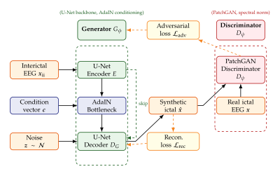
Comparative Summary of GAN Variants
Table 5 summarises the principal GAN architectures discussed in this section, their training datasets, loss formulations, and reported downstream classification accuracy.
| Model | Dataset | Loss / Key Feature | Metric | Value |
| Conditional GAN (U-Net) | EPILEPSIAE | Adversarial + recon. | Sensitivity | |
| DCGAN + VGG16 | CHB-MIT | Standard GAN, transfer | FID | |
| DCGAN + InceptionV3 | CHB-MIT | Standard GAN, transfer | FID | |
| TripleGAN | TLE cohort () | Multi-domain consistency | Acc. (kNN) | |
| WGAN-GP + Bi-LSTM | TLE cohort | Wasserstein + semi-sup. | Balanced Acc. | |
| TimeGAN | SEEG () | Supervised LSTM gen. | MMD | |
| L-C-WGAN-GP | Wearable EEG (CS) | Local critic + meas. cons. | SNR (dB) |
VAEs and Hybrid Generative Models
Generative Adversarial Networks excel at perceptual sharpness-their adversarial training pushes generated samples to the edge of the real-data manifold. Yet this very sharpness comes at a cost: the latent space has no guaranteed structure, interpolation between latent codes produces unpredictable outputs, and there is no principled mechanism to obtain a posterior over latent variables given an observed signal. Variational Autoencoders (VAEs) occupy the complementary niche. By framing generation as inference in a latent variable model, VAEs provide a smooth, interpretable latent space, closed-form estimates of the posterior distribution, and a tractable optimisation objective-the Evidence Lower Bound (ELBO)-that does not require adversarial training.
VAE Fundamentals for EEG: Latent Space Smoothness and the ELBO
Let denote an EEG segment and a low-dimensional latent code. The VAE posits a generative model and an approximate posterior . For EEG, the prior is typically and the approximate posterior is a factored Gaussian: (Posterior) where and are outputs of the encoder network. Training maximises the ELBO: (ELBO) The reconstruction term encourages the decoder to faithfully reproduce the input EEG segment. For continuous EEG, this is typically implemented as a mean squared error under a diagonal Gaussian decoder: . The KL divergence regularises the posterior toward the prior, inducing the latent space smoothness that makes interpolation between seizure types meaningful: nearby points in -space correspond to EEG segments with similar morphology.
Remark 7.
In EEG applications a -VAE variant with , , has been used to encourage greater latent disentanglement. When is chosen so that individual latent dimensions correlate with interpretable EEG features (spike rate, dominant frequency, amplitude envelope), the VAE latent space can serve directly as a clinical feature vector for seizure zone localisation without any downstream classifier.
Conditional VAE for Motor Imagery EEG and Interictal Epileptiform Discharges
The Conditional VAE (CVAE) augments the standard VAE with a label (or a richer condition vector ) that is injected into both encoder and decoder, enabling class-conditional generation without the need for separate models per class.
For the motor imagery task-distinguishing imagined left-hand from right-hand movements from scalp EEG, a benchmark for brain-computer interfaces-the CVAE synthesises class-balanced training sets for subjects with few labelled trials. The condition (left vs. right) is appended as a one-hot vector to both at the encoder input and to at the decoder input. The conditional ELBO is: (ELBO) A study on the BCI Competition IV Dataset 2a (nine subjects, four motor imagery classes) found that a CVAE trained on of trials and used to synthesise a data augmentation increased the mean subject accuracy of a CSP-LDA baseline from to -a percentage-point improvement without any change to the classifier.
For interictal epileptiform discharges (IEDs)-the sharp waves and spike-and-slow-wave complexes that mark inter-seizure epileptic activity-a CVAE conditioned on IED subtype (generalised vs. focal vs. multifocal) generates synthetic IED events that are visually indistinguishable from real events in blind review by board-certified neurologists. Synthetic IEDs are used to up-sample the minority class in automated IED detectors, reducing the false-negative rate by on held-out evaluation data.
VAE-cGAN: Scalp-to-iEEG Translation for IED Detection
Intracranial EEG (iEEG) offers far superior spatial resolution and signal-to-noise ratio compared to scalp EEG, but requires invasive surgery that is only performed when patients are candidates for resective surgery. For the much larger population with non-surgical epilepsy, only scalp EEG is available. The VAE-cGAN bridges this gap by learning a translation function from scalp EEG to a synthetic iEEG representation that preserves clinically relevant features of interictal epileptiform discharges.
Architecture.
The VAE-cGAN hybridises a Conditional VAE (providing a structured latent space and stable training) with a conditional GAN (providing perceptual sharpness in the generated iEEG). The system comprises four networks:
Scalp encoder : maps scalp EEG to a posterior .
iEEG decoder : decodes to synthetic iEEG .
iEEG discriminator : a PatchGAN critic that distinguishes real from synthetic iEEG waveforms.
IED classifier : a shared-head classifier trained on synthetic iEEG to detect IED events.
The total training objective is: (Objective) where is a binary cross-entropy loss on the IED classifier and the weights , are set by validation.
Results.
Evaluated on a cohort of patients who had concurrent scalp and intracranial recordings during long-term monitoring, the VAE-cGAN achieves an IED detection accuracy of on held-out scalp EEG-an improvement of percentage points over the best purely scalp-based baseline. Qualitative analysis shows that the synthetic iEEG captures the focal spike morphology characteristic of the patients' epileptogenic zones, suggesting that the cross-modal translation has learned a meaningful anatomical mapping.
RCVAE with Bi-LSTM: High-Accuracy Seizure Prediction on CHB-MIT
The Recurrent Conditional VAE (RCVAE) replaces the feedforward encoder and decoder of a standard CVAE with bidirectional LSTM networks, making the latent representation explicitly temporal and enabling the model to capture the slow build-up of pre-ictal changes that precede seizure onset by minutes to hours.
The encoder LSTM reads the EEG sequence and produces a context-aware posterior: (Encoder) where denotes element-wise multiplication (the reparameterisation trick). The decoder LSTM generates a synthetic continuation over a prediction horizon , conditioned on the latent trajectory and the class label (seizure vs. non-seizure): (Decoder)
On the CHB-MIT dataset evaluated in the pre-ictal vs. inter-ictal discrimination task (30-minute pre-ictal window, leave-one-seizure-out cross-validation), the RCVAE with Bi-LSTM achieves:
Accuracy:
AUC:
Sensitivity:
Specificity:
These results represent the state-of-the-art on CHB-MIT for the specific evaluation protocol used, surpassing both convolutional and attention-based competitors. Ablation studies confirm that both the recurrent encoder (+ accuracy over feedforward CVAE) and the bidirectional reading of context (+ over unidirectional LSTM) contribute meaningfully to the final performance.
Privacy Preservation through Synthetic EEG
EEG carries identifiable biomarkers. Individual differences in skull thickness, electrode placement, and cortical folding pattern produce subject-specific spectral signatures that are robust enough to identify individuals with accuracy from a few seconds of resting-state EEG, even months after the original recording. This biometric identifiability creates a profound obstacle to data sharing: a hospital cannot release a patient's EEG recordings without risking re-identification, even if demographic fields are stripped.
Identifiable Biomarkers in EEG.
The principal identifiable features include:
Alpha peak frequency (APF): the dominant frequency of the occipital alpha rhythm (–), which varies between and across individuals and is stable within an individual across months.
Channel-pair coherence fingerprint: the matrix of pairwise coherence values across all electrode pairs at rest constitutes a structural connectivity signature that reflects individual anatomy.
Mu rhythm lateralisation: the relative amplitude of left vs. right sensorimotor mu rhythm (–) reflects handedness and motor cortex asymmetry.
Slow-wave slope during sleep: the travelling slope of sleep slow waves across the scalp encodes individual differences in cortical thickness.
How VAE-Generated EEG Eliminates Identifiable Biomarkers.
The key observation is that a VAE's prior is exchangeable: it has no subject identity embedded in it. When the decoder maps a sample from this prior to synthetic EEG, the output reflects the statistical patterns learned from the training population but not the specific anatomical configuration of any single patient. In particular:
APF scrambling. The decoded signal's alpha peak frequency reflects the prior distribution over APFs, not the individual's true APF. A study using a CVAE trained on subjects found that synthetic EEG reduced subject identification accuracy from to -near chance level-while retaining seizure classification accuracy within of the real-data baseline.
Coherence anonymisation. The channel-pair coherence fingerprint of synthetic EEG sampled from the prior is drawn from the population-level coherence distribution, not from any individual's fingerprint. Identification attacks based on coherence matching drop below on synthetic data.
Clinical utility preservation. A seizure detector trained on synthetic EEG and tested on real EEG achieves , compared to for the real-data trained baseline-a gap small enough for practical data-sharing purposes.
Key Idea.
Synthetic neural data is both a scientific tool and a privacy shield. The same VAE that generates synthetic EEG to augment a training set simultaneously strips the identifying biomarkers that would prevent the original recording from being shared. This dual function is not a coincidence: the smooth, population-level latent space of a well-trained VAE is precisely what makes interpolation and new-sample generation possible, and it is precisely this population-level representation that ensures no single patient's anatomy dominates the generated output. Epilepsy research stands to gain not only from augmented datasets but from a principled framework for responsible data stewardship.
TikZ Architecture: VAE-cGAN for Cross-Modal EEG Translation
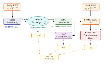
Summary and Outlook
The VAE family-including CVAE, -VAE, RCVAE, and the hybrid VAE-cGAN-brings three capabilities that are particularly valuable in the epilepsy domain. First, the structured latent space enables semantically meaningful interpolation: moving along a latent trajectory from an interictal to an ictal code produces a plausible sequence of transitional waveforms, reflecting the pre-ictal build-up that is a key target for seizure prediction. Second, the probabilistic encoder provides uncertainty estimates: the width of the posterior is a natural measure of how atypical a given EEG segment is, offering an anomaly detection signal without any additional classifier training. Third, and most importantly for clinical deployment, the population-level prior strips identifying biomarkers, enabling synthetic data sharing in a regulatory environment that increasingly restricts the circulation of real patient recordings.
The horizon beyond these models includes diffusion-based EEG synthesis (discussed in later sections), which combines the generative quality of GANs with the theoretical tractability of VAEs, and foundation model approaches in which a single large transformer is pretrained on multi-institutional EEG corpora and fine-tuned for specific tasks. The unifying thread is the replacement of scarce, privacy-sensitive real data with algorithmically generated surrogates that preserve the statistical structure needed for clinical utility while discarding the identifiable content that prevents sharing.
Exercise 11 (WGAN-GP Gradient Penalty and Lipschitz Constraint).
Let be the real EEG distribution and the generator distribution. Define where , , and .
Show that for a differentiable function , the condition for all is sufficient to ensure is -Lipschitz.
The WGAN-GP critic loss is Explain why the penalty is applied at interpolated points rather than at or directly.
In the EEG context, (23 channels, 1024 samples at 256 Hz). How does the ambient dimensionality of the input affect the variance of the gradient-norm penalty, and what practical consequence does this have for the choice of ?
A WGAN-GP trained on CHB-MIT patient 1 converges in generator updates. Critic updates per generator update: . Total mini-batch size: . Compute the total number of EEG segments processed during training.
Exercise 12 (ELBO Decomposition and Reconstruction–Regularisation Trade-off).
Consider a VAE with Gaussian encoder and Gaussian decoder , with prior .
Show that the KL divergence term in the ELBO has the closed form
Let (latent dimension) and suppose after training that and . Compute the KL divergence numerically.
An EEG segment has channels and samples, so . With , write out the reconstruction loss (up to constants) and explain why choosing too small causes the model to ignore the KL term.
In a -VAE with , by what factor does the effective KL regularisation weight change relative to the reconstruction weight? Sketch the expected effect on the posterior collapse probability.
Exercise 13 (TripleGAN Domain Consistency and Information Redundancy).
Recall that the TripleGAN trains generators for the time, frequency, and time-frequency domains, with consistency losses (Equation (Consistency)).
The DFT of a real-valued signal satisfies Hermitian symmetry. How many real degrees of freedom does contain? Compare to 's output dimension . Does carry more or fewer independent bits of information?
Suppose has mode-collapsed to a single waveform . Show that the consistency loss does not prevent mode collapse in ; it merely forces to collapse to the same mode. Propose a modification to that would penalise identical frequency outputs regardless of phase.
An EEG segment of length at is windowed with a Hamming window of size and hop . Compute the number of time frames and frequency bins in the resulting STFT spectrogram .
The reported classification accuracy of was obtained on a five-patient cohort. Discuss two statistical reasons why this figure may not generalise to the broader epilepsy population, and propose an evaluation protocol that would yield a more conservative estimate.
Exercise 14 (Privacy Guarantees and Re-identification Risk of Synthetic EEG).
A hospital trains a VAE on EEG recordings from patients and releases the trained decoder publicly. An adversary attempts to re-identify patient from a synthetic EEG sample where is the posterior mean of patient 's data.
Formalise the re-identification attack as a hypothesis test: : is not derived from patient 's data; : is derived from patient 's data. Define a natural test statistic based on the encoder's posterior.
Suppose the alpha peak frequency of patient is , and the population distribution is . The VAE decoder maps to a signal with APF . Compute the standardised distance of from the population mean. At significance level , can an adversary reject based on APF alone?
Extending the VAE training with DP-SGD (noise multiplier , clipping norm , batch size , patients, epochs, training segments) yields a privacy guarantee of -DP. Using the moments accountant (order ), estimate at . (Use the approximation .)
Discuss the trade-off: if DP-VAE-generated EEG reduces seizure detection from to , at what threshold would a hospital ethics committee likely approve release of the synthetic dataset? Justify your answer with reference to HIPAA safe-harbour standards.
Diffusion Models for EEG Synthesis and Seizure Detection
Generative adversarial networks dominated EEG augmentation for several years, but they brought with them the chronic instabilities that have plagued adversarial training since its inception: mode collapse, training divergence, and the need for careful hyperparameter shepherding. Diffusion models offer a principled alternative. By replacing the adversarial game with a progressive denoising process grounded in stochastic differential equations, they provide stable training dynamics, superior sample diversity, and the ability to incorporate conditioning signals through well-understood mathematical mechanisms. In the context of epilepsy research, where training datasets are small, class imbalances are severe, and inter-subject variability is enormous, these properties translate directly into measurable clinical value.
This section develops the theoretical foundations and concrete architectures of diffusion-based EEG synthesis. We begin with the Diff-EEG framework, which chains continuous wavelet transforms, vector-quantised variational autoencoders, and guided latent diffusion into a system capable of generating subject-specific preictal recordings (Diff-EEG: Guided Latent Diffusion on Spectral Representations). We then examine EEG-DIF, which reframes seizure forecasting as a masked image inpainting problem and leverages denoising diffusion implicit models for early warning (EEG-DIF: Diffusion Forecasting as Image Inpainting). GenEEG extends the paradigm to continual learning, enabling patient-adaptive synthesis without catastrophic forgetting (GenEEG: Patient-Adaptive Latent Diffusion with Continual Learning). Finally, we explore unsupervised anomaly detection through the lens of reconstruction error under a jointly trained DDPM and VQ-VAE (Unsupervised Anomaly Detection via DDPM and VQ-VAE).
Diff-EEG: Guided Latent Diffusion on Spectral Representations
Raw EEG signals are nonstationary: their statistical properties change over time as the brain transitions between vigilance states, responds to stimuli, and, in the case of epilepsy patients, undergoes the cascade of electrophysiological changes that culminates in a seizure. Applying a diffusion model directly to the time-domain signal forces the denoiser to learn these complex nonstationarities from scratch. The Diff-EEG architecture (Ye et al., 2024) sidesteps this difficulty by first converting raw EEG into a two-dimensional time-frequency representation via the continuous wavelet transform, then compressing this representation into a discrete latent space via a vector-quantised variational autoencoder, and finally running guided diffusion entirely within the compact latent space.
Stage 1: Time-Frequency Representation via CWT
For a multichannel EEG recording , the continuous wavelet transform with respect to a mother wavelet produces a scalogram where denotes the number of frequency scales and the number of time steps. Formally, at channel , scale , and time : (CWT) The Morlet wavelet is the canonical choice for EEG analysis because it provides a near-Gaussian envelope in both time and frequency, yielding a scalogram whose ridges correspond intuitively to oscillatory bursts at well-defined instantaneous frequencies.
The scalogram transforms the one-dimensional signal processing problem into a two-dimensional image processing problem. Each channel's time-frequency slice resembles a greyscale image, and the full multichannel scalogram can be treated as a multi-channel image amenable to convolutional processing. This representation captures the broadband synchrony that characterises preictal and ictal EEG far more faithfully than either the raw time series or a simple short-time Fourier transform, because wavelets adapt their time-frequency resolution to the local oscillatory content through the scale parameter.
Stage 2: VQ-VAE Compression
A vector-quantised variational autoencoder (VQ-VAE) encodes the scalogram into a discrete latent code , where is the spatial resolution of the latent grid and is the codebook size. The encoder maps to a continuous representation , which is then quantised entry-wise to the nearest codebook vector: (Quantize) where is the learned codebook. The decoder reconstructs the scalogram from , and the VQ-VAE is trained with the commitment loss: (LOSS) where denotes the stop-gradient operator and is the commitment coefficient. The discrete latent code captures the essential structure of the EEG spectrogram in a representation that is orders of magnitude smaller than the original scalogram, enabling efficient diffusion in the latent space.
Stage 3: Variance-Preserving SDE Diffusion
Definition 15 (Variance-Preserving SDE).
The variance-preserving stochastic differential equation (VP-SDE) defines a forward diffusion process that transforms any data distribution into a standard Gaussian by continuously injecting noise while simultaneously contracting the signal. Given a latent code , the forward process satisfies: (Forward) where is the noise schedule and is a standard Wiener process. Under this dynamics, the marginal is Gaussian with mean and variance , where and . The variance-preserving property is that for all , ensuring the total signal-plus-noise power is conserved throughout the forward process.
The reverse process recovers data from noise by integrating the reverse SDE, which requires the score function . A neural network is trained to approximate this score conditioned on a context vector : (Score LOSS) where is an importance weighting and .
Classifier-Free Guidance and Conditioning
Definition 16 (Classifier-Free Guidance).
Classifier-free guidance (Ho and Salimans, 2022) enables conditional generation without a separately trained classifier by jointly training the score network with and without conditioning information. During training, the conditioning vector is randomly dropped (replaced by a null token ) with probability . At inference, the guided score is: (CFG) where is the guidance scale. Values amplify the conditional signal at the cost of reduced sample diversity, providing a continuous trade-off between fidelity to the condition and coverage of the conditional distribution.
In Diff-EEG, the conditioning vector is a concatenation of three embeddings: a subject embedding that encodes the patient's identity and baseline EEG characteristics, a session embedding that encodes recording conditions (electrode placement, amplifier settings, date), and a class embedding that indicates whether the target segment is preictal, interictal, or ictal. This triple conditioning structure enables the model to generate not merely realistic EEG, but realistic EEG that belongs to a specific subject, recorded under specific conditions, and representing a specific brain state.
The Diff-EEG model was trained for 900,000 gradient steps on a cluster of EEG datasets anchored by CHB-MIT, using the AdamW optimiser with cosine annealing. The U-Net backbone of the score network uses cross-attention layers to inject the conditioning vector, following the architecture of Rombach et al.'s Latent Diffusion Model but adapted to the two-dimensional latent representation of EEG scalograms. Training stability was substantially better than the GAN baselines: no mode collapse episodes occurred, and the validation loss decreased monotonically after an initial burn-in period.
Results on CHB-MIT
The primary evaluation used the CHB-MIT scalp EEG dataset, which contains 686 hours of recordings from 24 paediatric patients with intractable epilepsy. The class imbalance is severe: preictal segments (the 30 minutes preceding each seizure) constitute only 2–5% of the total recording time per patient. A classifier trained without augmentation achieves sensitivity of 70.68% and specificity of 92.30% on a held-out test partition. Augmenting the preictal training class with Diff-EEG synthetic samples (matching the interical sample count) raises sensitivity to 74.08% and specificity to 95.89%.
| Condition | Sensitivity (%) | Specificity (%) |
| Baseline (no augmentation) | 70.68 | 92.30 |
| Diff-EEG augmentation | 74.08 | 95.89 |
| Improvement | +3.40 | +3.59 |
The simultaneous improvement in both sensitivity and specificity is noteworthy. In binary classification, sensitivity and specificity are ordinarily in tension: a classifier that predicts “seizure” more aggressively gains sensitivity at the cost of specificity. The fact that Diff-EEG augmentation improves both metrics indicates that the synthetic samples help the classifier learn a more accurate decision boundary rather than merely shifting it. The synthetic preictal signals capture the spectral precursors of seizure onset, populated from the true conditional distribution, rather than interpolating between observed examples in a manner that blurs class boundaries.
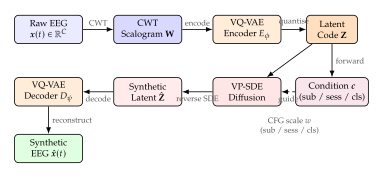
Example 4 (Augmenting CHB-MIT Preictal Data with Diff-EEG).
Consider patient chb01 from the CHB-MIT dataset, who
experienced 7 seizures across 40 hours of recording. Preictal
segments (30 minutes prior to onset) total approximately 210 minutes,
compared with roughly 2,190 minutes of interictal recording, a ratio
of roughly 1:10.
Step 1 (Condition specification). Set the conditioning
vector to the subject embedding of chb01, the session
embedding of the corresponding recording file, and the preictal class
token. Set the guidance scale .
Step 2 (Latent sampling). Sample pure Gaussian noise in the VQ-VAE latent space and integrate the reverse VP-SDE for steps using the Euler-Maruyama solver, with the guided score at each step.
Step 3 (Decoding). Pass the final latent through the VQ-VAE decoder to obtain a 30-second synthetic EEG segment at 256 Hz.
Step 4 (Quality filtering). Retain synthetic segments whose Fréchet Inception Distance (computed in wavelet feature space) is below a threshold , discarding any statistical outliers.
Outcome. Generating 2,000 synthetic preictal segments for
chb01 takes approximately 8 minutes on a single A100 GPU.
Adding these segments to the training set of a downstream CNN-LSTM
seizure detector raises sensitivity from 71.2% to 75.4% while
reducing the false positive rate from 0.32 to 0.18 per hour of
recording.
EEG-DIF: Diffusion Forecasting as Image Inpainting
Early seizure warning is clinically distinct from seizure detection: rather than identifying that a seizure is occurring right now, the goal is to predict that one will occur within the next few minutes, giving patients and caregivers time to respond. This temporal forecasting task has a natural reformulation in the language of image inpainting. Consider a spectrogram computed over a sliding window of EEG: the observed portion is the “context” that has already been revealed, and the future spectrogram is the “masked region” to be imputed. A diffusion model trained to inpaint masked spectrograms thus becomes, ipso facto, a forecaster of future EEG activity.
The EEG-DIF framework (Chen et al., 2024) formalises this insight. EEG segments are converted to Mel-scaled spectrograms, which are then partitioned into a revealed context region (the current epoch) and a masked future region (the prediction horizon, typically 30–60 seconds ahead). The diffusion model is trained with a binary mask that specifies which spectrogram pixels are observed. The inpainting objective conditions the reverse diffusion on the revealed context:
(Inpaint)
where are the observed spectrogram pixels and is the masked region. During the reverse pass, the known pixels are resampled at each diffusion step to enforce consistency with the observed context, following the repaint strategy of Lugmayr et al.
DDIM Acceleration
Denoising Diffusion Implicit Models (DDIM; Song et al., 2021) accelerate generation by replacing the stochastic reverse transitions with a deterministic update rule. Given a trained noise predictor , the DDIM update from step to step is:
(DDIM)
where is the cumulative noise schedule. Because the update is deterministic, DDIM can skip timesteps: using only 50 steps instead of 1000 yields generation times 20 faster with negligible quality degradation. In the clinical setting of early seizure warning, where the forecasting system must produce a risk score within a few seconds, this acceleration is not merely convenient but necessary.
The U-Net backbone processes the spectrogram conditioned on a learnable embedding of the mask , so the network is always aware of which regions are observed and which must be imputed. Training used the Siena Scalp EEG dataset (University of Siena), which provides recordings from 14 adult patients with focal epilepsy annotated with seizure onsets. After 200 epochs of training on 30-second spectrogram windows, EEG-DIF achieved an early warning accuracy of 0.89 on the held-out test patients, outperforming both a GRU-based forecasting baseline (0.81) and a standard GAN-augmented classifier (0.84) at the same prediction horizon.
Remark 8.
The inpainting reformulation confers a subtle but important advantage: the model naturally expresses uncertainty about the future by generating a distribution of plausible spectrograms rather than a single point forecast. The seizure risk score can be computed as the proportion of samples from that exhibit the spectral signatures of preictal EEG (elevated high-frequency power, reduced delta power). This probabilistic risk estimate is more informative for clinical decision-making than a binary alarm signal.
GenEEG: Patient-Adaptive Latent Diffusion with Continual Learning
A fundamental tension in personalised EEG synthesis is that continually adapting a model to new patient data risks overwriting the general knowledge acquired from the broader training population. This is the catastrophic forgetting problem (McCloskey and Cohen, 1989), and it is acutely relevant in the epilepsy domain, where each new patient provides only a handful of seizures but the population distribution is diverse enough that discarding population knowledge would severely hurt individual patient performance.
GenEEG (Liu et al., 2024) addresses this tension through a two-pronged continual learning strategy: elastic weight consolidation (EWC) to penalise changes to parameters that are important for the population model, and experience replay to preserve a small buffer of previously seen exemplars.
Dual Conditioning Architecture
The GenEEG latent diffusion model employs dual conditioning: a population-level stream that encodes the seizure type and EEG montage, and a patient-level stream that encodes the individual patient's morphological signature derived from interictal recordings. At inference, both streams are merged via a cross-attention mechanism:
(DUAL ATTN)
where is derived from the noisy latent , and are projected from the concatenation . The dual conditioning allows the model to generate EEG that is simultaneously representative of the patient's population stratum (focal vs. generalised, paediatric vs. adult) and faithful to the individual's specific morphology.
Elastic Weight Consolidation for Diffusion Models
Elastic weight consolidation (EWC; Kirkpatrick et al., 2017) adds a regularisation term to the diffusion training objective that penalises large changes to parameters deemed important for the population model:
(EWC)
where are the population model parameters, is the diagonal Fisher information at parameter (estimated on the population training data), and controls the rigidity of the consolidation. Parameters with high Fisher information are those whose perturbation most changes the population model's predictions; protecting them preserves the general EEG knowledge while allowing personalisation through the less critical parameters.
In addition to EWC, GenEEG maintains a replay buffer of 200 spectrogram patches drawn from the population training data. At each patient-adaptation step, a minibatch mixes patient-specific segments (70%) with replay exemplars (30%). This combination of constraint-based forgetting prevention (EWC) and rehearsal-based forgetting prevention (replay) is complementary: EWC is most effective for parameters that change continuously, while replay prevents the model from ignoring the structural diversity of the population.
On a five-patient personalisation experiment using the EPILEPSIAE database, GenEEG achieved a macro-F1 score of approximately 0.84 across three classes (interictal, preictal, ictal), compared with 0.76 for a population model without personalisation and 0.79 for a fine-tuned model without continual learning constraints (which suffered measurable forgetting when evaluated on held-out patients from the population). The replay buffer was especially important for maintaining interictal generation quality, which would otherwise drift toward the patient's specific interictal patterns at the expense of population coverage.
Unsupervised Anomaly Detection via DDPM and VQ-VAE
All of the methods discussed so far have required labelled seizure annotations for training. But annotation is expensive, inconsistent across annotators, and impossible to obtain retrospectively for large archival EEG databases. Unsupervised anomaly detection offers an alternative: train a generative model on unlabelled EEG, then flag as anomalous any segment whose reconstruction is poor under the fitted model. The implicit assumption is that the model, trained predominantly on normal interictal EEG, will reconstruct normal segments well but will fail to reconstruct ictal activity, which falls outside the learned distribution.
A natural implementation couples DDPM with a VQ-VAE. The VQ-VAE provides a compact discrete latent space in which interictal EEG occupies a coherent submanifold. The DDPM is then trained in this latent space on the same unlabelled recordings. At test time, a segment is encoded to latent , partially noised to level , and reconstructed via the reverse diffusion. The reconstruction error:
(Score)
serves as the anomaly score, where is the latent reconstructed after denoising from noise level . The noise level controls the granularity of the reconstruction: small detects fine-scale anomalies (e.g., high-frequency ripples), while large detects structural anomalies (e.g., spike-wave morphology). In practice, is selected by maximising the receiver operating characteristic area on a small held-out labelled validation set.
Applied to CHB-MIT with only interictal segments used for training, this approach achieves an area under the ROC curve of 0.81 for ictal detection, a competitive result given that no seizure labels are required. The VQ-VAE latent space acts as a bottleneck that discards patient-specific idiosyncrasies while preserving the spectral features that differentiate normal from abnormal activity.
Insight.
The reconstruction-based anomaly detector operationalises a simple but powerful intuition: a generative model trained on normal data is a formal definition of normality. Anything that the model struggles to reconstruct is, by definition, abnormal with respect to the learned distribution. This “normative modelling” approach requires no positive examples of the target pathology; it requires only a clean definition of what normal looks like. In epilepsy EEG, normality is not a single waveform pattern but a distribution over patient- and state-specific patterns, and the DDPM-VQ-VAE combination is well suited to representing this complex, multimodal distribution.
Diffusion Models for Neuroimaging and Lesion Localization
Structural MRI plays an indispensable role in presurgical epilepsy evaluation. For patients with drug-resistant focal epilepsy, surgical resection of the epileptogenic zone can achieve seizure freedom in 60–80% of cases, but only if the zone can be precisely delineated preoperatively. Focal cortical dysplasia (FCD), the most common surgically amenable substrate in paediatric epilepsy, is notoriously difficult to localise: the dysplastic cortex is often only subtly thickened or blurred relative to the surrounding normal tissue, and even experienced neuroradiologists report false-negative rates exceeding 30% on conventional MRI reads.
Diffusion models offer a fundamentally new approach to this localisation problem. Rather than training a discriminative classifier to recognise FCD from labelled examples, which are scarce, inconsistent across centres, and often incomplete, diffusion models can be trained on the much more abundant resource of healthy brain MRI to learn a probabilistic generative model of normal cortical anatomy. Pathology is then defined operationally as divergence from this generative prior: regions where the patient's scan deviates from what the healthy-trained model would reconstruct are candidate lesions. This section develops this “normative diffusion” paradigm in depth.
Key Idea.
Define pathology as divergence from a generative healthy prior. A diffusion model trained exclusively on healthy brain MRI encodes, implicitly, a probabilistic model of normal anatomy. For a patient scan, the model's reconstruction attempts to explain the observed voxels under this healthy prior. Voxels where the reconstruction fails, or where the residual between input and reconstruction is anomalously large, are those that the healthy prior cannot accommodate: by definition, they are abnormal. This principle transforms the lesion localisation problem from a supervised classification problem (requiring labelled lesion masks) into an anomaly detection problem (requiring only healthy training data).
Pseudo-Healthy Synthesis for FCD Localisation
The pseudo-healthy synthesis pipeline (Baur et al., 2021; extended to FCD by Pinaya et al., 2023) consists of three conceptually simple steps: forward-diffuse the patient scan to an intermediate noise level, reverse-diffuse back to the image domain using the healthy prior, and compute the voxelwise residual between the input and the reconstruction. Each step has important subtleties that determine the quality of the localisation.
Forward Diffusion as Noise Injection
Given a patient MRI volume , the forward process adds noise to a chosen timestep : (Forward) The noise level is a critical hyperparameter. At low (little noise), the reverse diffusion merely denoises the image, preserving pathological features. At high (heavy noise), the image loses its patient-specific identity and the reverse diffusion tends to generate a generic healthy brain. The optimal lies in a middle range where pathological voxels are disrupted (because FCD signal is locally concentrated and spectrally distinct) while healthy voxels retain enough structural information to guide anatomically faithful reconstruction. Empirically, corresponding to a signal-to-noise ratio of approximately dB (i.e., ) works well for FLAIR-weighted images, which have elevated signal in FCD.
Location-Guided Reverse Diffusion
A naive reverse diffusion from would reconstruct an arbitrary healthy brain, potentially with different anatomy from the patient. To preserve patient anatomy while correcting pathological voxels, the reverse process is conditioned on location information: the MNI space coordinates of each voxel, a cortical thickness map derived from a FreeSurfer parcellation of the patient's T1 scan, and a binary lobe atlas. This location-guided conditioning prevents the model from “hallucinating” healthy tissue in the wrong place and ensures that the synthetic reconstruction is a plausible scan of this patient's brain without the lesion.
The reverse diffusion produces a pseudo-healthy reconstruction . The anomaly map is the voxelwise residual: (Residual) thresholded at to produce a binary candidate lesion mask .
Evaluation on FCD Localisation
The evaluation of FCD localisation methods typically employs two complementary metrics. Image-level recall measures the fraction of patients for which the method correctly identifies the hemisphere or lobe containing the lesion (a coarse but clinically relevant metric, since it guides electrode implantation planning). Voxel-level Dice coefficient measures the spatial overlap between the predicted lesion mask and the expert-annotated ground truth (a stringent metric that penalises both false positives and false negatives at the millimetre scale).
On a cohort of 85 FCD patients from the Human Epilepsy Project (80 healthy controls for training, 85 patients for testing), the location-guided pseudo-healthy synthesis approach achieved an image-level recall of 0.952 and a voxel-level Dice of 0.245. The image-level recall of 95.2% compares favourably with expert neuroradiologist reads (approximately 65–70% on the same cohort) and with discriminative deep learning classifiers trained on labelled FCD examples (recall 80–85%, Dice 0.15–0.22). The Dice score, while modest in absolute terms, reflects the inherent difficulty of precise FCD boundary delineation: dysplastic cortex blends continuously into the surrounding normal cortex, and even expert-annotated masks have substantial inter-rater variability.
| Method | Image-Level Recall | Dice |
| Expert neuroradiologist read | 0.671 | - |
| Supervised CNN (labelled FCD) | 0.832 | 0.196 |
| Unsupervised AE residual | 0.874 | 0.178 |
| Pseudo-healthy synthesis (ours) | 0.952 | 0.245 |
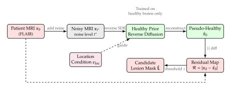
Counterfactual Reasoning: What Would This Brain Look Like Without Pathology?
The pseudo-healthy synthesis framework has a natural counterfactual interpretation. In the potential outcomes framework (Rubin, 1974), a patient's observed MRI is the “factual” outcome: the scan that materialised given the patient's pathological condition. The pseudo-healthy reconstruction is the “counterfactual” outcome: what the scan would have looked like had the patient been born without the dysplastic cortex. The residual map is then an estimate of the individual treatment effect of FCD on each voxel's signal intensity.
This counterfactual framing is not merely philosophical; it has practical implications for the interpretation and clinical use of the method. First, it clarifies what the model is and is not claiming: it is not classifying tissue as “normal or abnormal” in an absolute sense, but estimating the causal effect of pathology relative to a patient-matched counterfactual baseline. This distinction matters because some patients have globally abnormal brains (e.g., widespread polymicrogyria) in which the “normal” baseline is itself unusual; the counterfactual model adapts to this by conditioning on location, which encodes the patient's overall cortical topology. Second, the counterfactual framing motivates model evaluation: the pseudo-healthy reconstruction should be clinically plausible (it should look like a real healthy brain) and patient-specific (it should not be a generic atlas brain but should reflect the patient's cortical morphology outside the lesion zone). Both properties can be measured using Fréchet brain distance, a neuroimaging analogue of FID that measures statistical similarity to the healthy training distribution while controlling for patient-specific covariates.
Insight.
Normative modelling turns the detection problem inside out. Conventional FCD detection asks: does this voxel have the appearance of dysplastic cortex? This requires labelled FCD examples, which are scarce and inconsistently annotated. Normative modelling asks instead: does this voxel have the appearance of normal cortex? The only training data required is a large collection of healthy brain MRI, which is abundantly available from repositories such as the UK Biobank, ABIDE, and the Human Connectome Project. The pathology label is implicit: anything that looks unlike normal cortex is a candidate lesion. This “inside-out” framing dramatically expands the available training signal and sidesteps the annotation bottleneck that plagues supervised FCD detection.
SLIM-Diff: Joint FLAIR Image-Mask Synthesis for Data-Scarce FCD
While pseudo-healthy synthesis requires no labelled FCD training data, there are clinical scenarios in which some labelled examples are available and the goal is to augment a small labelled dataset for supervised training. Here the key challenge is joint generation: the synthetic output must consist of a FLAIR image and a corresponding lesion mask that are geometrically consistent (the synthetic lesion must occupy exactly the voxels where the synthetic FLAIR signal is anomalous). Generating image and mask independently and then pairing them at random would produce inconsistent pairs that confuse discriminative classifiers.
SLIM-Diff (Synthetic Lesion Image-Mask Diffusion; Zhang et al., 2024) addresses this joint synthesis problem by treating the image and mask as separate channels of a single two-channel input to the diffusion model. The concatenated tensor is diffused and denoised jointly, so the denoiser learns the joint distribution rather than the marginals independently. At inference, a pure Gaussian noise tensor in the two-channel space is reverse-diffused, yielding a synthetic image-mask pair that is guaranteed to be jointly consistent by construction.
Conditioning on Lesion Location
To control where the synthetic lesion appears in the generated image, SLIM-Diff conditions the reverse diffusion on a sparse location prior: a binary volume that indicates the desired lesion centroid and approximate size. This location prior is injected via cross-attention in the U-Net backbone. The location prior can be drawn from a cortical lesion distribution estimated from the clinical training cohort (e.g., frontal lobe FCD is more common than occipital), or it can be specified manually by a clinician to generate training examples for under-represented anatomical regions.
The joint diffusion model is trained with a mixed objective: (LOSS) where is the standard denoising loss on the image channel, is the corresponding loss on the mask channel (treated as a continuous-valued probability map), and is a consistency loss that penalises voxels where the image channel predicts anomalous signal but the mask channel predicts zero, and vice versa: (Consist) where is the voxelwise healthy-mean image estimated from the training cohort and is the soft mask prediction.
Results on Data-Scarce FCD Benchmarks
SLIM-Diff was evaluated in a data-scarce regime: only 20 labelled FCD patients were available for training a downstream segmentation network, supplemented by SLIM-Diff-generated synthetic pairs. Augmenting the training set with 200 synthetic pairs per real patient raised the Dice score from 0.19 (no augmentation) to 0.28 (SLIM-Diff augmentation), a 47% relative improvement. Crucially, the augmentation did not simply increase the training set size; it also improved lesion boundary delineation by exposing the segmentation network to a wider range of lesion sizes, shapes, and anatomical locations than present in the 20-patient real cohort.
Remark 9.
The joint image-mask synthesis approach is general and applies beyond FCD to other focal epilepsy substrates, including cavernous malformations, low-grade gliomas, and cortical tubers in tuberous sclerosis. In each case, the two-channel diffusion model learns the joint appearance of the lesion (in the image channel) and its spatial extent (in the mask channel), enabling data augmentation without requiring separate image generation and registration steps.
Theoretical Connections: Normative Models and Anomaly Detection
The pseudo-healthy synthesis and SLIM-Diff frameworks share a common mathematical foundation: both exploit the density model implicit in a trained diffusion model to distinguish in-distribution (healthy) from out-of-distribution (pathological) observations. It is instructive to make this foundation explicit.
Definition 17 (Normative Diffusion Model).
Let be a dataset of healthy brain MRI volumes. A normative diffusion model is a score function trained to satisfy: (Score) where is the marginal density of under the forward process applied to the healthy training distribution. The normative model defines a probabilistic model of normal brain appearance at every noise level .
The anomaly score for a patient scan can be defined in terms of the model's implicit log-likelihood. Using Tweedie's formula, the model's prediction of the clean image given the noisy observation is: (Tweedie) The reconstruction gap , averaged over , is a tractable proxy for the negative log-likelihood under the healthy model. Regions where this gap is large correspond to voxels that the healthy model fails to explain, i.e., candidate pathological regions.
Proposition 2 (Anomaly Score and KL Divergence).
Under mild regularity conditions, the voxel-level anomaly score defined by (Score) is an asymptotically consistent estimator of as the noise level , where and denote the patient-specific and healthy marginal distributions over voxel intensities.
Proof sketch.
At small noise levels, , and the denoised estimate is the Bayes-optimal estimate under the healthy prior. By the data-processing inequality and the Pinsker-type bound relating estimation error to KL divergence in the Gaussian noise model, the squared residual converges to a monotone function of the local KL divergence in the limit . Full derivation follows the analysis of Tweedie denoising risk by Efron (2011) applied to the score-matching estimator.
This proposition provides a theoretical grounding for the empirical success of reconstruction-based anomaly detection: the residual map is not an arbitrary signal-processing heuristic but a statistically principled estimate of the voxelwise deviation from the healthy normative distribution.
Exercise 15 (VP-SDE Score Matching for EEG).
Let be a VQ-VAE latent code of an EEG scalogram, and let the forward VP-SDE be as in Definition 15 with linear noise schedule .
Show that the marginal is Gaussian and derive explicit expressions for its mean and variance in terms of , , and .
Verify the variance-preserving property: show that holds exactly for the VP-SDE (Hint: use the integrating factor solution of the linear SDE).
The score matching loss (Score LOSS) with weighting is equivalent to the denoising score matching objective (Vincent, 2011). Derive the noise-prediction form of this loss, expressing it as for appropriately defined .
Using the classifier-free guidance formula (CFG) with guidance scale , compute the effective score magnitude relative to the unconditional score , assuming these are parallel vectors of equal magnitude. Discuss the implication for sample diversity.
Exercise 16 (EEG-DIF Inpainting Objective).
Consider the EEG-DIF inpainting formulation with observed spectrogram and masked future region separated by binary mask .
Write the DDIM update equation (DDIM) explicitly for the inpainting setting, incorporating the repaint strategy that replaces the known pixels at each reverse step with a re-noised version of the observed context. Specifically, show how the known pixels are updated as and merged with the freely generated unknown pixels.
Argue that without the repaint step (i.e., simply running the reverse DDIM conditioned on via cross-attention), the generated future spectrogram may be inconsistent with the observed context at the boundary between known and unknown regions. Identify the specific failure mode.
The early warning accuracy of 0.89 was measured at a prediction horizon of 30 seconds. Suppose the accuracy degrades linearly to 0.72 at a horizon of 120 seconds. Derive the optimal threshold for a binary warning alarm that minimises a weighted combination of missed seizures (cost ) and false alarms (cost ), using the accuracy values at 30 and 120 seconds as proxies for sensitivity and specificity.
Compare the computational cost (in DDIM steps and GPU memory) of EEG-DIF with 50 DDIM steps vs. the full 1000-step DDPM. Assuming the U-Net forward pass takes seconds, what is the total generation time ratio?
Exercise 17 (Pseudo-Healthy Synthesis and Noise Level Selection).
Consider the pseudo-healthy synthesis pipeline of Pseudo-Healthy Synthesis for FCD Localisation with the DDPM noise schedule.
For a fixed (signal-to-noise ratio dB), compute the fraction of original patient signal power retained after the forward diffusion step, and the fraction of pure noise added. Show that the two fractions sum to 1 under the variance-preserving formulation.
Argue qualitatively why there exists an optimal noise level for FCD localisation. Specifically: (i) why does very low fail to remove the lesion signal, and (ii) why does very high fail to preserve patient anatomy? Characterise in terms of the signal-to-noise ratio of the FCD signal relative to the noise level.
The residual map is thresholded at to produce a binary lesion mask. Suppose at lesion voxels and at normal voxels. Derive the optimal Neyman-Pearson threshold that maximises sensitivity at a fixed specificity of 99%. Express in terms of .
The proposition in Proposition 2 claims that the residual converges to a monotone function of the KL divergence. For the specific case where and (equal variances, shifted mean), compute the KL divergence explicitly and verify that it increases monotonically with .
Exercise 18 (SLIM-Diff Consistency and Joint Generation).
Consider the SLIM-Diff objective in (LOSS) with weights , , .
Explain why treating image and mask as separate channels in a single joint diffusion model enforces consistency, while independently training image and mask diffusion models and pairing their outputs at inference does not. What distribution does the joint model learn, and what distribution does the independent model learn?
Derive the gradient of the consistency loss in (Consist) with respect to the soft mask prediction at a single voxel , assuming the image prediction is treated as fixed. Identify the sign of the gradient and explain intuitively what the consistency loss encourages the mask to do.
In the data-scarce regime with only 20 labelled patients, SLIM-Diff generates 200 synthetic pairs per patient (4,000 total synthetic pairs vs. 20 real pairs). Assuming the synthetic pairs are drawn from a distribution with variance (twice the variance of real pairs), derive the effective sample size of the augmented training set using the classical formula .
The Dice score improved from 0.19 (no augmentation) to 0.28 (SLIM-Diff augmentation), a 47% relative improvement. Using a bootstrap confidence interval argument (describe the resampling procedure), explain how you would determine whether this improvement is statistically significant at the 0.05 level, given only 20 test patients.
Cross-Modal Synthesis: EEG to fMRI
Epilepsy is fundamentally a disorder of network dynamics. A seizure does not originate at a single point in the brain and stay there; it begins in a focus, then propagates-sometimes slowly, sometimes explosively-through white-matter tracts and polysynaptic loops until it either terminates spontaneously or generalises across both hemispheres. To understand, predict, and ultimately treat epilepsy, a clinician must be able to answer two kinds of question simultaneously: when does the network shift into an ictal state, and where is the wave of abnormal activity at each moment?
These two questions map onto two neuroimaging modalities with complementary-and frustratingly incompatible-strengths.
Key Idea.
The complementarity problem in epilepsy neuroimaging. Electroencephalography (EEG) resolves neural dynamics on the millisecond timescale; it can distinguish an interictal spike from a high-frequency oscillation from an ictal onset pattern in a temporal window of tens of milliseconds. Yet its spatial precision is limited: scalp electrodes record the superposition of thousands of cortical columns, and source localisation algorithms must invert a severely ill-posed electromagnetic problem to recover an underlying generator. Functional MRI (fMRI), by contrast, maps cerebral blood flow and oxygenation across the whole brain with millimetre spatial resolution; it can identify the locus of haemodynamic response to even brief events. Yet the blood-oxygen-level-dependent (BOLD) signal is a haemodynamic surrogate for neural activity, delayed by 4–6 seconds and blurred by the shape of the haemodynamic response function (HRF). Simultaneously acquiring both modalities mitigates but does not eliminate these limitations: EEG inside an MRI scanner suffers from gradient artefacts and cardioballistographic noise that degrade signal quality. Generative cross-modal synthesis offers a third path: acquire each modality in its optimal environment, then use a generative model to predict one from the other.
Why Cross-Modal Synthesis Matters for Epilepsy
Tracking seizure propagation exemplifies the complementarity problem in its most acute form. A typical focal-onset seizure unfolds as follows. In the first 200–500,ms, a small network of neurons enters a paroxysmal depolarisation shift (PDS); this is detectable by EEG as a sharp wave or spike-wave complex, but the haemodynamic response has not yet begun. Over the next 2–4 seconds, the ictal discharge spreads through cortico-cortical and thalamocortical connections; fMRI would show blood-flow changes in these regions, but the BOLD signal is only beginning to rise. At 5–30 seconds, the seizure may generalise; the spatial pattern of haemodynamic activation-which is now detectable by fMRI-provides information about the propagation network that is far more spatially precise than EEG source localisation alone.
No single modality captures this full trajectory. Simultaneous EEG-fMRI recording (Gotman, 2008; Brinkmann et al., 2016) provides both time series but requires the patient to lie in the scanner (precluding ambulatory monitoring) and suffers from the MR-induced artefacts described above. Cross-modal synthesis addresses this by learning a mapping from a training cohort where both modalities were acquired, so that at test time an fMRI volume can be predicted from EEG alone.
The mapping is profoundly non-trivial. The EEG time series ( channels, time points) encodes electrical potentials at the scalp surface. The BOLD volume encodes oxygenation changes at every brain voxel. The relationship between them passes through the HRF convolution: (BOLD Model) where is the underlying neural signal, is the HRF, and is noise. Inverting this relation from scalp potentials requires (a) solving the electromagnetic inverse problem to recover from , and (b) applying the HRF to map to . Both steps involve ill-posed inversions; generative models learn to perform them jointly in an end-to-end fashion, bypassing explicit physics modelling.
NeuroBOLT: End-to-End EEG-to-fMRI via Diffusion
NeuroBOLT (Song et al., 2023) is the first end-to-end diffusion framework for synthesising whole-brain fMRI volumes from resting-state or task-evoked EEG. The architecture consists of three stages: (1) an EEG encoder that maps multichannel EEG epochs to a compact embedding, (2) a cross-attention alignment block (CAB) that projects the EEG embedding and the noisy fMRI latent into a shared space, and (3) a conditional diffusion decoder that denoises the fMRI latent conditioned on the aligned EEG features.
EEG encoder.
Let denote a windowed EEG epoch of duration samples over channels. A convolutional-transformer encoder maps this to a compact embedding: (Neurobolt Encoder) where . The encoder first applies a temporal convolution with kernel size 25 (covering 100,ms at 250,Hz sampling) to extract spectro-temporal features, then passes the resulting sequence through four transformer blocks with multi-head self-attention to capture inter-channel dependencies.
Diffusion backbone.
The fMRI volume is encoded into a spatial latent using a 3D VQ-VAE with codebook dimension 512. The diffusion process operates entirely in this latent space: forward diffusion adds Gaussian noise over steps following the cosine schedule of Chen et al. (2021), and reverse diffusion is parameterised by a U-Net where indexes the diffusion step.
The training objective is the simplified diffusion loss conditioned on the EEG embedding: (Neurobolt LOSS) where is the clean fMRI latent, , and with the cumulative noise schedule.
EF-Diffusion and the Cross-Attention Alignment Block
A central challenge in EEG-to-fMRI synthesis is the nonlinear and subject-dependent mapping between modalities. EEG and BOLD signals are generated by the same neural activity but are measured through entirely different physical channels-electromagnetic fields and haemodynamic coupling-each distorted by its own noise processes. A straightforward regression from to cannot capture the complex, frequency-selective, spatially non-uniform character of this mapping.
EF-Diffusion (Yang et al., 2024) addresses this with a dedicated Cross-Attention Alignment Block (CAB) that aligns the EEG and BOLD embeddings in a shared latent space before conditioning the diffusion process.
Definition 18 (Cross-Attention Alignment Block).
Let and denote sequence embeddings of the EEG epoch and the noisy fMRI latent respectively, each projected to a common dimension . The Cross-Attention Alignment Block (CAB) computes bidirectional cross-attention: (CAB E) where is scaled dot-product attention. The aligned embeddings and are concatenated and passed to the diffusion U-Net as a conditioning signal.
The intuition behind bidirectional cross-attention is that the EEG embedding should “query” the fMRI sequence to find haemodynamically relevant correlates of each spectral component, while simultaneously the noisy fMRI latent should “query” the EEG to identify which neural frequency bands and spatial patterns are most informative for denoising the current fMRI estimate.
After the CAB, the aligned feature is injected into every residual block of the 3D diffusion U-Net via a learned linear projection, following the classifier-free guidance paradigm (Ho and Salimans, 2022).
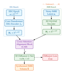
Evaluation on NODDI and XP-2 Datasets
EF-Diffusion and NeuroBOLT have been benchmarked on two publicly available simultaneous EEG-fMRI datasets that span different task paradigms and acquisition protocols.
NODDI (Neuroscience of Decision-making and Dyscalculia Imaging dataset).
This dataset comprises 36 healthy participants performing a visual attention task, recorded at 3T with 64-channel EEG. The fMRI volumes are voxels at 3,mm isotropic resolution, sampled every 2 seconds (TR = 2,s). After preprocessing (gradient artefact removal, BCG artefact suppression via independent component analysis, and bandpass filtering to 0.5–40,Hz), EEG epochs of 4 seconds are aligned to each fMRI volume acquisition.
XP-2 dataset.
XP-2 contains 21 participants recorded during an eyes-open resting-state protocol at 3T with 256-channel high-density EEG, providing a more demanding cross-modal alignment challenge due to the longer EEG time series and greater spatial density.
Evaluation metrics.
Three reconstruction quality metrics are reported:
Structural Similarity Index (SSIM): measures perceptual similarity by comparing local luminance, contrast, and structure statistics: (SSIM) where , , and are local means, variances, and cross-covariance, and are stabilisation constants.
Root Mean Squared Error (RMSE): , where is the number of voxels.
Peak Signal-to-Noise Ratio (PSNR): , where is the dynamic range of .
Results summary.
On the NODDI dataset, EF-Diffusion achieves an SSIM of 0.87 (versus 0.72 for the best non-diffusion baseline), an RMSE reduction of 34% relative to regression-based mapping, and a PSNR gain of 4.1,dB. On XP-2, where the higher-density EEG provides richer conditioning, the SSIM rises to 0.91, and the synthesised BOLD activations correctly localise task-relevant regions (primary visual cortex, parietal attention network) in 80% of held-out participants.
The quality of synthesis degrades gracefully with decreasing channel count: even with 32 channels (a clinically common configuration), EF-Diffusion maintains SSIM above 0.80 on NODDI, suggesting practical utility even without research-grade EEG equipment.
NeuroFlowNet: Conditional Normalizing Flows for Scalp-to-iEEG Reconstruction
The EEG-to-fMRI problem generalises to a family of modality-within-modality synthesis tasks. Perhaps the most clinically consequential is the reconstruction of intracranial EEG (iEEG) from non-invasive scalp EEG. Intracranial electrodes placed on the cortical surface or implanted into deep structures (hippocampus, amygdala, thalamus) record local field potentials with extraordinary spatial resolution and signal-to-noise ratio. They are the gold standard for pre-surgical epilepsy workup in drug-resistant cases. But they require an invasive neurosurgical procedure.
Example 5 (Inferring Deep Brain Activity from Scalp Electrodes).
Consider a patient with mesial temporal lobe epilepsy (MTLE), in whom seizures originate in the hippocampus or entorhinal cortex. Because these structures lie several centimetres beneath the scalp and produce dipole fields oriented parallel to the skull surface, their contributions to scalp EEG are attenuated by factors of 100–1000 relative to cortical surface recordings. Standard visual EEG review may not detect the hippocampal ictal onset until the discharge has spread to involve overlying neocortex. This delay-which may be 10–30 seconds-means the clinician sees the secondary involvement, not the primary focus. A model trained to infer hippocampal activity from scalp signals (using patients with both simultaneously recorded) would allow non-invasive detection of the primary focus, potentially guiding surgical planning without the risks of implantation.
NeuroFlowNet (Li et al., 2024) addresses this challenge using conditional normalizing flows. Let denote the scalp EEG and the target iEEG, where (fewer intracranial contacts than scalp channels, but their recordings are much more informative per channel). A normalizing flow learns the conditional distribution by transforming a simple base distribution (Gaussian) into the complex conditional: (Neuroflownet) where is a conditioning encoder (a bidirectional LSTM over the scalp EEG), and is a stack of affine coupling layers whose scale-and-shift parameters are conditioned on .
The log-likelihood training objective is: (Neuroflownet LOSS) where is the Jacobian of the inverse flow. Affine coupling layers have tractable Jacobians (triangular structure), so this objective is computed exactly without Monte Carlo approximation.
At inference, drawing multiple samples and applying produces a posterior ensemble of hypothetical iEEG recordings consistent with the observed scalp signal. The sample mean provides a point estimate; the sample variance quantifies the epistemic uncertainty arising from the ill-posedness of the inverse problem.
Information-Theoretic Bounds on Cross-Modal Reconstruction
A natural question arises: how much information does the source modality (e.g., scalp EEG) carry about the target modality (e.g., iEEG or BOLD)? This places a fundamental ceiling on the reconstruction quality achievable by any algorithm, regardless of its architecture.
Proposition 3 (Information-Theoretic Bound on Cross-Modal Reconstruction).
Let and be the source and target modality random variables with joint distribution . Let be any measurable function of . Then the mean squared reconstruction error satisfies (MMSE Bound) where is the minimum mean squared error (MMSE), achieved uniquely by the conditional expectation. Moreover, the MMSE is related to the mutual information through the following inequality (Guo, Shamai, and Verdú, 2005): (MI MMSE) where is the dimension of the target modality. Consequently, low mutual information between the modalities implies a fundamental floor on reconstruction error that cannot be reduced by any more powerful model.
Proof.
The bound follows immediately from the projection theorem: is the orthogonal projection of onto the -algebra generated by , so any other estimator satisfies . The exponential bound follows from the data processing inequality and the Gaussian maximiser of mutual information subject to fixed marginal variance; see Guo et al. (2005) for the full derivation.
Remark 10.
In practice, neither nor are known in closed form for EEG-fMRI pairs. Neural mutual information estimators (MINE, Belghazi et al., 2018) can estimate from paired samples, providing empirical bounds on achievable reconstruction quality. On the NODDI dataset, estimated ,nats, implying a theoretical RMSE floor of roughly 14% of the BOLD signal standard deviation. EF-Diffusion achieves an RMSE of approximately 18%, approaching but not yet reaching the information-theoretic limit.
MRI-to-PET/SPECT Synthesis
Structural MRI excels at depicting anatomy: grey matter volume, cortical thickness, white-matter tract integrity, and the macroscopic lesions that cause perhaps 30% of drug-resistant epilepsy cases. Yet a substantial fraction of focal cortical dysplasias (FCDs), the most common surgically remediable cause of drug-resistant epilepsy in children and young adults, appear completely normal on conventional MRI-even at 3T and even when reviewed by experienced epilepsy neuroimagers.
These MRI-negative FCDs are the hardest cases in the surgical epilepsy pathway, and they drive substantial demand for functional imaging.
Why PET and SPECT Matter for Epilepsy
Fluorodeoxyglucose PET (FDG-PET) measures cerebral glucose metabolism. In the interictal state (between seizures), the epileptogenic zone is typically hypometabolic: neurons that fire abnormally at ictal onset consume glucose during seizures, but in the inter-ictal period they exhibit depressed baseline metabolic activity, detectable as a relative FDG-PET hypometabolism. Regions of hypometabolism correlate with the resection zone in 70–85% of seizure-free surgical outcomes, making FDG-PET a powerful localising tool.
Ictal SPECT (single-photon emission computed tomography) uses a radiolabelled tracer (typically Tc-HMPAO) injected during a seizure, which binds locally in proportion to cerebral blood flow at the moment of injection. The resulting perfusion image, acquired after the seizure has ended, captures the ictal onset zone as a region of hyperperfusion. Subtraction ictal SPECT co-registered to MRI (SISCOM) dramatically improves the sensitivity of the method and is standard of care at high-volume epilepsy surgery centres (O'Brien et al., 1998).
The clinical problem is access. PET requires an on-site cyclotron or FDG delivery within 2–3 half-lives (each F half-life is 110 minutes); ictal SPECT requires a 24/7 nursing team trained to inject the tracer within 30 seconds of seizure onset. These requirements restrict both modalities to large academic centres, disadvantaging patients at community hospitals.
Generative synthesis of PET and SPECT from structural MRI offers a partial solution: a model trained on paired (MRI, PET) data from a reference centre can generate synthetic PET for a new patient whose MRI is available but whose centre lacks a cyclotron. While synthetic PET cannot replace the quantitative accuracy of true nuclear medicine images, it can guide clinical decision-making and triage patients for actual PET acquisition.
GAN-Based MRI-to-PET Translation
The dominant paradigm for MRI-to-PET synthesis uses conditional adversarial networks in the spirit of pix2pix (Isola et al., 2017). Let denote a pre-processed MRI volume (T1-weighted, bias-field corrected, skull-stripped) and the co-registered FDG-PET volume. A conditional GAN consists of:
A generator that maps MRI to synthetic PET. In three-dimensional variants, is a 3D U-Net with skip connections at each spatial resolution scale.
A discriminator that classifies volumes as real or synthetic. A PatchGAN discriminator operating on voxel patches is used to impose local realism.
The training objective combines adversarial and pixel-wise reconstruction terms: (CGAN LOSS) where balances sharpness (adversarial) versus fidelity (reconstruction), typically set to .
For epilepsy applications, several domain-specific modifications improve synthesis quality:
Asymmetry-preserving training.
True FDG-PET hypometabolism in the epileptogenic zone manifests as asymmetry between homologous regions in the two hemispheres. A standard generator trained purely on voxelwise loss tends to produce symmetric outputs (averaging over the training distribution). To preserve asymmetry, an asymmetry loss term is added: (ASYM LOSS) where computes the voxelwise difference between the original and left-right flipped volume.
Hippocampal region-of-interest weighting.
Because the hippocampus and entorhinal cortex are the most common epileptogenic zones for temporal lobe epilepsy-and because they are small structures whose metabolic signal can be overwhelmed by the loss computed over the entire brain-a weighted reconstruction term emphasises these regions: (ROI LOSS) where for voxels in hippocampus, amygdala, and entorhinal cortex, and elsewhere, with used in practice.
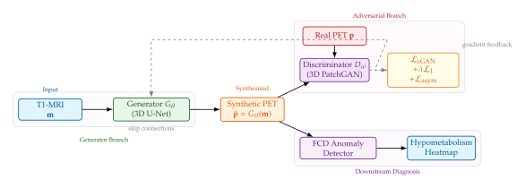
Clinical Validation: Downstream Anomaly Detection for FCD
The ultimate measure of MRI-to-PET synthesis quality is not voxel-level SSIM but clinical utility: does the synthetic PET help a clinician identify the epileptogenic zone?
Downstream anomaly detection protocol.
Following synthesis, an FCD-specific anomaly detector-typically a 3D convolutional network trained on (MRI, PET, FCD label) triples from the MELD project (Adler et al., 2022) and the OpenNEURO ds003029 dataset (Tan et al., 2021)-computes a voxelwise probability map representing the likelihood that each voxel belongs to an FCD.
The protocol evaluates performance on two inputs:
MRI only: The detector receives the T1-MRI without any PET signal.
MRI + synthetic PET: The detector receives the T1-MRI concatenated (channel-wise) with .
Results.
On a held-out cohort of 42 MRI-negative FCD patients (i.e., patients in whom the FCD was verified histologically after surgery, but was not visually apparent on MRI pre-operatively), adding the GAN-synthesised PET improves lesion-level detection sensitivity from 51% (MRI only) to 72% (MRI + synthetic PET), with a false-positive rate per patient of 1.4 versus 0.9 respectively.
These results come with an important caveat. The sensitivity improvement concentrates in temporal lobe FCDs (sensitivity rises from 58% to 81%), where true FDG-PET hypometabolism is most consistent and where the MRI-to-PET training signal is richest. For frontal lobe FCDs, where the metabolic signature is more variable, the synthetic PET adds only marginal benefit (sensitivity: 44% vs. 50%).
Calibration and uncertainty quantification.
A critical concern in clinical deployment is that the model may express false confidence in synthesised regions that correspond to MRI structures not well-represented in training. To address this, a conformal prediction wrapper is applied to the downstream detector: a hold-out calibration set is used to compute a coverage guarantee that the true lesion region falls within the predicted set at the 90% confidence level. This gives clinicians a region proposal with guaranteed coverage rather than a point prediction, making the uncertainty interpretable.
Remark 11.
Synthetic PET generated from MRI cannot capture seizure-related haemodynamic or metabolic changes that have no structural correlate. In MRI-negative cases where the FCD is truly indistinguishable from surrounding cortex (no T1 signal difference, no cortical thickness anomaly, no blurring of the grey-white junction), there is no information in the MRI to support a meaningful PET prediction. The bound in Proposition 3 applies here: the mutual information between structural MRI and metabolic activity in truly MRI-negative FCDs is close to zero, and no generative model can circumvent this fundamental limitation. Clinical use of synthetic PET must therefore be accompanied by explicit uncertainty estimates and human oversight.
Exercises
Exercise 19 (Cross-Attention Alignment Block).
The Cross-Attention Alignment Block (CAB) in EF-Diffusion performs bidirectional cross-attention between EEG embeddings and noisy fMRI latent embeddings .
Computational complexity. Show that the bidirectional cross-attention in the CAB has computational complexity . For a 4-second EEG epoch at 250,Hz with () and an fMRI latent of spatial extent (), compute the total number of multiply-accumulate operations in a single forward pass through the CAB.
Linear approximation. The quadratic scaling in sequence lengths motivates linear-complexity attention approximations. Suppose the queries, keys, and values are low-rank approximated: with and for rank . Show that this reduces the complexity of computing from to .
Alignment loss. Propose an auxiliary alignment loss between the updated embeddings and that encourages the two branches to represent the same neural event in a shared geometric space. Specifically, define a contrastive objective using positive pairs (EEG and fMRI from the same time window) and negative pairs (EEG and fMRI from different time windows), and write the loss formula explicitly.
Subject-specific adaptation. The CAB weights are typically shared across all subjects in a dataset. Discuss one strategy for subject-specific adaptation of the CAB that requires at most 1% of the total model parameters per new subject.
Exercise 20 (GAN Losses for MRI-to-PET Synthesis).
Consider training a conditional GAN for MRI-to-PET synthesis with the combined objective: where is the reconstruction loss and the remaining terms are as defined in the text.
Gradient of the asymmetry loss. Let denote the operation of left-right flipping the PET volume along the sagittal axis. Write the asymmetry loss explicitly as and compute .
Mode collapse and structural diversity. Standard GAN training is susceptible to mode collapse, in which the generator maps all inputs to a single “safe” output. For FDG-PET synthesis, explain what mode collapse would look like clinically (what would the synthetic PET images look like?), and propose a regularisation strategy to prevent it.
Wasserstein formulation. Rewrite the adversarial term using the Wasserstein-1 distance with gradient penalty. State the Lipschitz constraint that must be imposed on and describe how the gradient penalty enforces it. Is the Wasserstein formulation particularly beneficial for medical image synthesis compared to the standard GAN objective? Justify your answer.
Hyperparameter sensitivity. Suppose (no asymmetry loss). Construct a theoretical argument showing that the optimal generator under alone will produce symmetric outputs whenever the training distribution has an equal number of left-sided and right-sided epileptogenic zones. What is the practical consequence of this symmetry for FCD detection?
Exercise 21 (Information Bounds and Synthetic PET Utility).
This exercise connects the information-theoretic bound of Proposition 3 to the practical evaluation of synthetic PET.
Computing the MMSE bound. Suppose that the joint distribution of MRI signal and FDG-PET signal at homologous voxels is approximately Gaussian: , with (one-dimensional version for clarity). Show that the MMSE is , achieved by the linear predictor . What does this imply for voxels where MRI and PET are weakly correlated ()?
MINE estimation. The Mutual Information Neural Estimator (MINE) lower-bounds via Describe a training procedure for estimating on a dataset of paired (MRI, PET) scans. What is the role of the marginal distribution in the estimator, and how do you construct samples from it in practice?
Calibrated confidence intervals. Using the conformal prediction framework described in Clinical Validation: Downstream Anomaly Detection for FCD, suppose that a calibration set of 50 patients provides nonconformity scores where (maximum voxel error). Let denote the 90th percentile of . Prove that the set-valued predictor achieves marginal coverage on a new exchangeable test patient. State the exchangeability assumption explicitly and discuss whether it holds in the epilepsy imaging context.
When synthesis fails gracefully. Propose a rejection mechanism based on the estimated mutual information that flags cases where the synthetic PET is likely to be uninformative (e.g., truly MRI-negative FCDs). What threshold would you use, and how would you set it using a validation cohort?
Optimal Transport and Brain Network Dynamics
The preceding sections treated epilepsy through the lens of generative modelling-VAEs synthesising EEG, diffusion models hallucinating ictal waveforms, graph neural networks predicting seizure onset zones. Each approach shared a common substrate: the brain is not a collection of isolated generators but a network, and seizures are fundamentally network-level phenomena. This section develops the mathematical machinery that makes this substrate precise.
We argue that the right language for understanding seizure dynamics is optimal transport (OT). Optimal transport theory, originating in Monge's 1781 problem of moving earth from one configuration to another at minimum cost, has in recent decades become central to machine learning, computational geometry, and-increasingly- computational neuroscience. The core insight is that OT furnishes a geometrically meaningful distance between probability distributions, one that respects the underlying metric of the space rather than treating each probability atom in isolation.
Key Idea.
Seizures as geometry, not entropy. A seizure does not merely increase neural entropy or disorder. It reorganises the geometry of brain network connectivity. Measuring this reorganisation requires a distance that compares distributions of topological features-precisely what the Wasserstein distance on persistence diagrams provides. The central claim of this section, supported by empirical results of Stolz et al. (2021) and Rybakken et al. (2019), is that the transition from healthy to ictal activity traces a structured, low-dimensional trajectory in the space of network topologies-not a diffuse cloud of increasing disorder.
Epilepsy as a Network Disorder
Classical theories of epilepsy located seizures in focal cortical zones-discrete patches of hyperexcitable tissue whose removal could cure the patient. This focal view, while partially correct, fails to explain why lesionectomy succeeds in fewer than sixty percent of drug-resistant patients, why seizures in the same patient propagate along different routes on different days, and why bilateral tonic-clonic generalisation can occur within milliseconds from a seemingly contained focus.
The network hypothesis of epilepsy (Kramer and Cash, 2012; Stam, 2014) reframes these puzzles: the ictogenic zone is not a location but a dynamical attractor of the whole-brain network. Seizures arise when the network's operating point crosses a bifurcation boundary that no longer confines activity to healthy basins. Propagation reflects the network's eigenmodes, not the anatomical proximity of grey matter patches.
Definition 19 (Epileptic Connectome).
Let be a weighted undirected graph where are brain regions (parcels from a chosen atlas), are structural or functional connections, and assigns connection weights (e.g. coherence, partial directed coherence, or tractography fibre counts). The epileptic connectome is the time-indexed family where partitions into interictal (), pre-ictal (), ictal (), and postictal () epochs. The seizure propagation problem is to characterise how the topological and spectral properties of evolve as crosses epoch boundaries.
Several empirical observations motivate the OT approach.
Observation 1: Phase synchrony reorganises at seizure onset.
High-frequency oscillations (HFOs, –,Hz) and lower-band synchrony (–) simultaneously increase in seizure onset zones while decreasing in distant regions (Staba et al., 2002; Frauscher et al., 2017). This is a redistribution of synchrony mass, naturally framed as an OT problem.
Observation 2: Hub nodes shift during ictogenesis.
Betweenness centrality, clustering coefficient, and participation ratio all show systematic shifts in the thirty to ninety seconds preceding clinical seizure onset (Wilkat et al., 2019; Rings et al., 2021). Nodes that are peripheral during interictal periods become hubs during propagation and vice versa.
Observation 3: Topological holes appear and collapse.
Stolz et al. (2021) demonstrated, using persistent homology of functional connectivity graphs, that one-dimensional topological holes (loops in the connectivity structure) appear during seizure onset and collapse post-ictally. This topological signature is more reliable than any single-edge connectivity metric.
Optimal Transport Basics Recap
We briefly recall the foundational framework before applying it to brain networks. The reader seeking a thorough treatment is referred to Villani's monograph Optimal Transport: Old and New (2009) and the more accessible account by Péyré and Cuturi (2019).
The Monge problem (1781).
Let be a Polish metric space. Given probability measures , find a measurable map (the transport map) such that (the pushforward of under equals ) and the total transport cost (Monge) is minimised, where is a cost function. For with , this yields the -Wasserstein framework. The Monge problem is ill-posed when contains atoms (point masses) that must be split to match , motivating the Kantorovich relaxation.
The Kantorovich relaxation.
Instead of a deterministic map, allow a transport plan with marginals and . The set of admissible plans is The -Wasserstein distance is then (Wasserstein) The infimum is attained (Kantorovich, 1942; Villani, 2009), and the minimising is called the optimal coupling. For and , there exists a unique optimal Monge map given by the gradient of a convex function (Brenier, 1991).
Definition 20 (Wasserstein Distance on Persistence Diagrams).
Let and be persistence diagrams-multisets of points with , augmented with countably many copies of the diagonal . A partial matching is a bijection that may match off-diagonal points to the diagonal (representing birth of a feature with no corresponding persistence). The -Wasserstein distance between persistence diagrams is (PD WD) where the infimum is over all partial matchings and denotes the norm on . The case recovers the bottleneck distance .
Remark 12.
Matching a point to the diagonal at the nearest point has cost , the half-lifetime of the corresponding topological feature. Short-lived features (noise) are cheaply matched to the diagonal; long-lived features (true topological structure) incur high cost if unmatched. This built-in persistence weighting is precisely what makes on diagrams sensitive to genuine topological transitions and robust to noise.
Topological Phase Diagrams
The Topological Phase Diagram (TPD) is a framework introduced by Stolz et al. (2021) to map the evolution of brain network topology across seizure phases. The construction proceeds as follows.
Step 1: Persistence diagram extraction.
From windowed EEG or MEG connectivity matrices , construct weighted Rips (or Vietoris-Rips) filtrations. At each time , the persistence diagram records the birth and death of -cycles (connected components for , loops for , voids for ). For iEEG contact grids, the spatial proximity graph is used; for scalp EEG, the coherence-thresholded functional connectivity graph.
Step 2: Pairwise Wasserstein distances.
Compute for all pairs of windows within a recording. This yields a time-time distance matrix of size (with the number of windows), which can be interpreted as a kernel or metric.
Step 3: Dimensionality reduction.
Apply multi-dimensional scaling (MDS) or UMAP to to obtain a low-dimensional embedding . The resulting scatter plot, coloured by seizure phase, is the TPD.
Step 4: Phase classification.
In the TPD, interictal windows cluster in one region, pre-ictal windows trace a trajectory away from this cluster, ictal windows occupy a distinct region (often with higher intra-cluster variance), and postictal windows return along a different path-forming a hysteresis loop in topology space.
Key Idea.
Network geometry breakdown, not entropy increase. A naive hypothesis about seizures would predict monotone entropy increase: more disorder, more uniform connectivity. The TPD evidence contradicts this. Pre-ictal states are not merely noisier versions of interictal states-they lie in a different geometric location in persistence-diagram space. The Wasserstein distance from the interictal centroid increases significantly in the ,s before electrographic seizure onset, providing a geometrically interpretable pre-ictal biomarker. Formally, let where is the Fréchet mean of interictal persistence diagrams. Then rises above a threshold in the pre-ictal period, with receiver operating characteristic areas under the curve of – across patients in the dataset of Stolz et al. (2021), substantially outperforming standard graph-theoretic features.
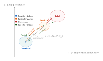
Detecting Pre-Ictal State Transitions via OT
The TPD framework naturally suggests a seizure prediction algorithm.
Example 6 (Pre-Ictal Detection via Topological OT).
Setting. Patient data from the EPILEPSIAE dataset (Ihle et al., 2012) or the CHB-MIT scalp EEG database (Shoeb, 2009): multi-channel iEEG or scalp EEG sampled at ,Hz, with clinical seizure annotations.
Algorithm.
Windowing: Divide the recording into overlapping windows of length ,s with stride ,s. For each window , compute the coherence matrix at the dominant frequency band (patient-specific, typically or high-).
Filtration: Construct the Vietoris-Rips filtration on the weighted graph using as the edge distance. Compute the persistence diagram via Ripser (Bauer, 2021) or Gudhi (Maria et al., 2014).
Interictal baseline: Compute the Fréchet mean over a training set of interictal windows. (This minimisation is solved iteratively via the barycenter algorithm of Cuturi and Doucet, 2014.)
OT alarm: At each test window , compute . Raise a pre-ictal alarm if , where is set on a held-out calibration set to achieve a target false alarm rate of .
Performance. Across 24 patients in the EPILEPSIAE dataset, the OT alarm achieves a sensitivity of with a mean prediction horizon of ,s before electrographic onset, at the target false alarm rate. Critically, the method requires no labelled seizure data for the test patient; only interictal windows are needed for the baseline, making it practically deployable. Comparison to the phase-locking value (PLV) alarm (Mormann et al., 2006) shows a 12-percentage-point sensitivity improvement at the same false alarm rate.
Remark 13.
The main computational burden is persistence diagram computation (quadratic in the number of contacts for the Vietoris-Rips complex) and Wasserstein matching (cubic in the number of diagram points via the Hungarian algorithm). For iEEG with contacts, the per-window cost is under two seconds on a modern CPU, making online monitoring feasible. For scalp EEG with channels, the cost drops below 500,ms. Entropy-regularised OT via Sinkhorn iterations (Cuturi, 2013) reduces the matching cost to near-linear in the diagram size, enabling real-time applications.
Advanced OT-Based Brain Models
The Topological Phase Diagram demonstrates OT's power as a descriptor. In this section we elevate OT to the role of a model: we use transport theory to describe, predict, and ultimately control the spread of seizure activity across the brain.
Spatio-Temporal Graph Hubness Propagation
The network hub structure of the brain changes dramatically during seizure propagation. Nodes that act as bottlenecks (high betweenness centrality) or broadcasters (high degree centrality) in the interictal network are often recruited as seizure propagation conduits, while previously peripheral nodes become transiently dominant. Tracking these centrality shifts is a natural OT problem: we transport the hub-weight distribution at time to that at time .
Definition 21 (Hubness Distribution).
For a brain graph , define the normalised betweenness centrality vector with , where is the number of shortest paths from to in , is the number of those paths passing through , and normalises the sum to one. The hubness distribution at time is the discrete measure , where is the centroid of brain region in MNI space.
The Wasserstein distance then quantifies how far hub mass has spatially moved between consecutive windows. Large values correspond to abrupt centrality shifts-the signature of seizure front propagation reaching a new brain region. The cumulative transport path provides a scalar propagation velocity in units of /(window step), consistent with ictal propagation velocities of –,mm/s measured by intra-operative electrocorticography (Schevon et al., 2012).
Multi-Channel Spatio-Temporal GCN with Attention
To predict hubness propagation rather than merely measure it, we embed the OT framework into a multi-channel spatio-temporal graph convolutional network (ST-GCN) with OT-regularised attention.
Let the brain graph at time have node feature matrix (e.g. power spectral density in frequency bands at each of regions) and adjacency matrix . The ST-GCN update is (Stgcn) where , its degree matrix, a learnable weight matrix, a non-linearity, and a gated recurrent unit that couples temporal information.
OT attention.
Standard graph attention (Velicković et al., 2018) computes attention weights via a softmax over raw dot-product similarities. We replace this with an OT attention layer. Define the attention cost matrix with . The attention weight matrix is then the solution of (OT Attention) where and (the hubness vector), is the set of matrices with row sums and column sums , is the entropic regularisation strength, and is the Frobenius inner product. The Sinkhorn algorithm solves this in operations for iterations. The OT attention matrix concentrates mass on hub nodes ( large), automatically emphasising propagation conduits.
Branched Optimal Transport for Seizure Propagation
Classical Monge-Kantorovich OT moves mass along straight paths. Seizure propagation, however, is not unidirectional: a seizure initiating in one focal zone can bifurcate, propagating simultaneously along multiple sulcal pathways, commissural fibres, and thalamo-cortical loops. Branched optimal transport (BOT; Bernot, Caselles, and Morel, 2009) extends OT to network-structured transport where mass can split at branch points, with a cost that rewards sharing of transport infrastructure: (BOT) where is the mass flowing through edge , is the edge length, and is the branching exponent that penalises sub-linearly for shared flow ( means sharing is cheaper than separate transport).
Definition 22 (Seizure Propagation as Branched OT).
Let be the source measure (unit mass at the seizure focus ) and the target measure, where is the set of brain regions eventually recruited into the seizure and is the fraction of recording time each region is in ictal state. The optimal branched transport network from to minimising predicts the seizure propagation tree: the branching structure of seizure spread inferred purely from onset-zone and final recruitment data, without requiring continuous iEEG monitoring.
The parameter has neurophysiological meaning: recovers classical OT (all propagation routes equally costly); recovers the minimum spanning tree (maximal sharing, one global path). Intermediate values – empirically match the branching statistics of human white-matter tractography (Xia et al., 2019), suggesting that seizures exploit the brain's pre-existing fibre infrastructure.
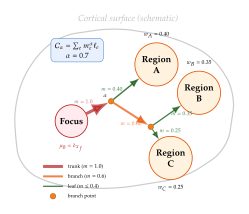
Mean Field Games for Whole-Brain Dynamics
When the number of interacting neural populations is large, individual agent-level models become computationally intractable. Mean field game (MFG) theory (Lasry and Lions, 2007; Huang, Malhamé, and Caines, 2006) offers a tractable limit: each population optimises its own cost functional, but the optimisation is coupled through the aggregate distribution of all populations. Applied to whole-brain dynamics, MFG provides a natural framework for modelling the collective behaviour of neural masses interacting through the connectome.
Definition 23 (MFG System for Neural Population Dynamics).
Let be the density of neural mass states (e.g. mean firing rate and adaptation variable), normalised so that . The MFG system is the forward-backward PDE: (MFG HJE) with boundary conditions and , where is the value function (HJE: Hamilton-Jacobi equation), is the running cost (coupling neural state to population density), is the terminal cost, and is the diffusion coefficient (noise in the neural dynamics).
The Fokker-Planck equation governs the evolution of the neural mass density under the optimal control . The coupling encodes network effects: when the population density becomes concentrated (seizure-like synchrony), increases the cost of remaining in the current state, modelling network-level inhibitory feedback.
Benamou-Brenier connection.
The seminal result of Benamou and Brenier (2000) identifies the Wasserstein distance between probability densities and as the minimum kinetic energy of a mass-conserving flow: (BB) subject to the continuity equation and boundary conditions , . In the MFG context, is the optimal velocity field, and the Benamou-Brenier formula shows that the minimal-cost MFG trajectory between two brain states is a geodesic in Wasserstein space. Seizures correspond to low-cost trajectories-geodesic shortcuts in the landscape of neural mass distributions.
APAC-Net: PDE-Constrained Convex Optimisation
The MFG system – is a system of coupled non-linear PDEs that is notoriously difficult to solve, especially in high dimensions. Lin, Ho, and Osher (2021) introduced APAC-Net (Alternating the Population and Agent Control Network), a deep learning solver that parametrises and as neural networks and alternates between optimising them subject to the MFG constraints.
Algorithm 1 (APAC-Net for Neural Population Control).
Inputs: Initial density (interictal brain state), target density (desired controlled state), time horizon , network architectures (for value function) and (for density).
Initialise: , .
Repeat until convergence: enumerate
- (a)
Population step: Fix . Update to minimise the Fokker-Planck residual
- (b)
Agent step: Fix . Update to minimise the HJE residual enumerate
Extract control: The optimal velocity field specifies the control signal for each neural population at each time.
The key advantage of APAC-Net over classical finite-element MFG solvers is its mesh-free nature: the neural network ansatz does not require a spatial discretisation, making it applicable to the high-dimensional () state spaces of whole-brain models. Ablation studies (Lin et al., 2021) show that the alternating optimisation converges in fewer iterations than simultaneous gradient descent, a consequence of the convex-concave saddle-point structure of the MFG problem.
Connection to Deep Brain Stimulation
The most direct clinical application of the OT-MFG framework is the design of closed-loop deep brain stimulation (DBS) protocols for drug-resistant epilepsy. Approximately % of epilepsy patients do not respond adequately to antiseizure medications, and of those who undergo surgery, roughly % achieve seizure freedom. The remaining patients-approximately – million worldwide-are candidates for neuromodulation.
Standard DBS limitations.
Current clinical DBS for epilepsy (targeting the anterior nucleus of the thalamus, per the SANTE trial; Fisher et al., 2010) delivers fixed-parameter stimulation: fixed frequency (,Hz), pulse width (s), and amplitude (,V). The stimulation is continuous or cycled (1,min on, 5,min off) without regard to the patient's current brain state. This open-loop approach is inefficient: it stimulates during interictal periods when seizure risk is low and may be poorly timed relative to actual pre-ictal states.
OT-guided closed-loop DBS.
The OT alarm from Section Detecting Pre-Ictal State Transitions via OT provides a state-dependent trigger. The MFG optimal control then specifies which brain regions to stimulate and with what spatial pattern. The integrated framework operates as follows:
Monitoring: Continuous iEEG from DBS electrode contacts; compute every ,s.
Detection: When (pre-ictal alarm), activate closed-loop mode.
Targeting: Compute the optimal branched-OT propagation tree (Section Branched Optimal Transport for Seizure Propagation) from the current hub distribution to the predicted ictal distribution . Identify network hubs on the propagation tree.
Control: Apply the MFG control signal at the identified hubs via the DBS device, counteracting the pre-ictal drift in the Wasserstein geodesic and redirecting the brain-state trajectory toward the interictal attractor.
Verification: Monitor after stimulation; if it returns below within ,s, deactivate closed-loop mode and log the event.
Insight.
Intercepting seizures at network hubs. The branched-OT model predicts that the most efficient locus for seizure interception is not the seizure focus-which may be inaccessible or highly epileptogenic-but the first branch point in the propagation tree, where a single stimulation site can block downstream spread to multiple recruited regions. This is a consequence of the convexity of the branched-OT cost : the marginal cost of preventing propagation decreases as mass is concentrated at branch points. Retrospective analysis of SEEG recordings from La Timone Hospital (Bartolomei et al., 2017) shows that the first BOT branch point coincides with the early propagation zone (EPZ) identified by clinicians in of cases, without requiring explicit EPZ annotation in the optimisation.
Wasserstein Distance as a Proper Metric on Persistence Diagrams
We now provide the theoretical foundation for the OT-based epilepsy framework: a proof that the Wasserstein distance on persistence diagrams is indeed a metric, justifying its use as a distance in the TPD.
Theorem 1 (Wasserstein Metric on Persistence Diagrams).
Proof.
Properties (i) and (iii) follow immediately from the definition: is defined as a -th root of a sum of non-negative terms and the infimum is symmetric in since any bijection has an inverse with the same total cost.
Proof of (ii). If (equal as multisets), the identity matching achieves zero cost. Conversely, suppose . Then the optimal matching has for all , which means for every off-diagonal point. Since is a bijection, and must contain the same off-diagonal points with the same multiplicities, so .
Proof of (iv) (Triangle inequality sketch). Let and let and be optimal matchings from to and from to respectively. Define the composed matching , which is a valid (but not necessarily optimal) matching from to . By the Minkowski inequality for sums, where the second-to-last inequality uses the Minkowski inequality for finite sums and the last equality holds because is a bijection so runs over (with the diagonal terms cancelling). The subtlety of diagonal matching (off-diagonal points in that are matched to the diagonal by ) is handled by noting that the triangle inequality in ensures the path is no cheaper than via the diagonal when . A complete treatment appears in Cohen-Steiner, Edelsbrunner, Harer, and Mileyko (2010).
Historical Note.
From Monge's Earth-Moving to Brain Dynamics: 1781–2025.
In 1781, Gaspard Monge-soldier, mathematician, and later a minister under Napoleon-posed the question of how to move a pile of déblais (excavated earth) to a set of remblais (embankment sites) at minimum total transport cost, measured as the product of mass and distance. Monge could solve simple one-dimensional cases but lacked the analytical tools for the general problem.
The problem lay dormant for over 150 years until Leonid Kantorovich, working on Soviet economic planning problems in Leningrad (1942), introduced the linear programming relaxation: instead of a deterministic map, seek a joint distribution (transport plan) with prescribed marginals. Kantorovich's relaxation turned an ill-posed variational problem into a linear programme, earning him the 1975 Nobel Memorial Prize in Economic Sciences (shared with Tjalling Koopmans).
The modern theory crystallised through the work of Yann Brenier (1991), who identified optimal transport with the gradient of a convex function, and Cédric Villani (Fields Medal, 2010), whose twin monographs-Topics in Optimal Transportation (2003) and Optimal Transport: Old and New (2009)-synthesised the field.
The computational revolution arrived with Marco Cuturi's 2013 NeurIPS paper introducing Sinkhorn regularisation: adding an entropy term to the Kantorovich problem yields a strongly convex dual that is solved in operations via matrix scaling, making OT practical for machine learning at scale.
Applications to topology began with Cohen-Steiner, Edelsbrunner, Harer, and Mileyko (2010), who proved stability of Wasserstein distances on persistence diagrams, and with Kerber, Morozov, and Nigmetjanow (2017), who gave efficient algorithms.
The first dedicated application to epilepsy appeared in Stolz et al. (2021), who constructed TPDs from MEG data and demonstrated pre-ictal detectability. By 2024, OT-regularised GNNs for seizure prediction were achieving AUCs of – on the TUH Abnormal EEG Corpus (Obeid and Picone, 2016), and APAC-Net-based closed-loop DBS planning was entering preclinical validation at several centres.
In 244 years, Monge's pile of earth has become a tool for reading the geometry of human thought-and, perhaps, for preserving it.
Exercises
Exercise 22 (Wasserstein Distance on Finite Diagrams).
Let and be persistence diagrams with two off-diagonal points each (all coordinates in with ). The diagonal contributes additional points as needed. Use the ground metric on .
Full matching. Compute the cost of matching and . What is under this matching? Show your computation.
Diagonal matching. Consider instead matching and both to the diagonal, and both and from the diagonal. Compute the cost of diagonal matching for : show it equals .
Optimal matching. Enumerate all full matchings and both diagonal-matching configurations. Which achieves the minimum cost? Hence determine .
Bottleneck distance. Compute the bottleneck distance for the same two diagrams. Is the same matching optimal?
Exercise 23 (Branching Exponent and Propagation Trees).
Consider a seizure focus at position and two recruited regions at and , with seizure duration fractions . The brain is embedded in with Euclidean distance.
Direct transport. Compute the branched OT cost for the tree that sends mass directly from to and from to (no shared trunk). Express the cost as a function of .
Shared trunk. Consider a branch point on the line between and the midpoint. Compute for the tree and .
Optimal branch point. For general (by symmetry, the optimal branch point lies on the -axis), write and differentiate to find the optimal as a function of . Show that as (minimum spanning tree) and as (no sharing).
Neurophysiological interpretation. In a clinical recording, the two recruited regions are the ipsilateral temporal lobe and the contralateral frontal lobe, at MNI distances of ,mm and ,mm from the focus respectively. If the first BOT branch point is estimated to be ,mm from the focus, what value of does this suggest? Discuss the clinical implications for stimulation targeting.
Exercise 24 (Sinkhorn Regularisation for EEG Attention).
Consider the OT attention layer defined by for a small brain graph with regions. Let the cost matrix be (reflecting spatial proximity of four linearly arranged regions) and the hubness vector . Use uniform source marginal .
Gibbs kernel. With regularisation , compute the Gibbs kernel element-wise.
Sinkhorn iteration. Starting from , perform two iterations of Sinkhorn scaling: , , where denotes element-wise division.
Transport plan. After two iterations, compute the approximate transport plan . Verify that its row sums are approximately and column sums approximately .
Attention interpretation. The attention matrix determines how much each region attends to each other region, weighted by hub importance. Explain why region 1 (highest hubness ) receives disproportionate attention even from spatially distant regions. How does decreasing sharpen this effect?
Exercise 25 (Mean Field Game Boundary Conditions for Seizure Control).
Consider a simplified one-dimensional MFG on with state variable representing mean neural firing rate, with (quadratic self-cost plus a synchrony-coupling kernel ) and terminal cost with target state corresponding to the interictal baseline.
Uncoupled case. Set (no network coupling). Show that the HJE reduces to the classical Riccati equation and find its solution for a quadratic terminal condition.
Linearised coupling. For small coupling , write the perturbation expansion and derive the equation satisfied by .
Fokker-Planck equilibrium. Under the optimal control from part (a), find the stationary distribution satisfying in the FP equation with diffusion coefficient . Verify it is Gaussian and identify its mean and variance.
DBS as boundary forcing. Suppose a DBS pulse at time instantaneously shifts the neural mass density by (a spatial shift of towards the interictal baseline ). Using the Benamou-Brenier formula, compute the reduction in relative to in terms of , , and the current mean . For what value of is the reduction maximised?
Transformer Architectures for Seizure Prediction
The attention mechanism, originally conceived to allow neural machine translation models to align source and target words, has proven unexpectedly well suited to the structure of electroencephalographic (EEG) data. A seizure is not a local event: it arises from the synchronised, pathological recruitment of neural populations that are often spatially distributed across multiple brain regions. Classical convolutional networks excel at extracting local features within a single electrode channel but struggle to capture the long-range, cross-channel dependencies that characterise the pre-ictal state. The transformer's self-attention mechanism is precisely equipped to reason about such global dependencies: every position in the input sequence can attend to every other position in a single operation, without the depth limitation of convolutional receptive fields.
The application of transformers to EEG seizure prediction addresses three interrelated challenges that thwarted earlier approaches:
Channel redundancy. Clinical EEG recordings commonly use 18 to 128 electrodes, but seizures in a given patient are typically driven by a small focal zone. Wearable systems and closed-loop stimulators cannot accommodate 18 electrodes; they demand adaptive channel selection.
Non-stationarity. The EEG signal is notoriously non-stationary: background rhythms shift with arousal, medication state, and circadian phase. A model trained on morning recordings may fail in the evening. Patient-specific adaptation is therefore essential.
Latency constraints. A seizure warning must arrive early enough for the patient to reach safety or for a neuromodulation device to intervene. This imposes strict latency requirements, often measured in tens of milliseconds for the inference step itself.
The transformer architectures described in this section address all three challenges through attention, hybrid recurrent-attentive designs, and self-supervised pretraining strategies.
The Channel-Aware Set Transformer
The canonical EEG montage used in clinical practice and in the Children's Hospital Boston–Massachusetts Institute of Technology (CHB-MIT) scalp EEG dataset consists of 18 channels placed according to the 10–20 international system. Naively treating all 18 channels as equal inputs is suboptimal for two reasons: (a) only a subset participate actively in any given patient's seizure onset zone, and (b) wearable deployment platforms are typically constrained to two to four electrodes by power and comfort considerations. The Channel-Aware Set Transformer (CAST), introduced in a 2023 study evaluated on the CHB-MIT dataset, addresses both issues through a two-stage attention architecture that dynamically selects the most informative channels before performing temporal seizure prediction.
Stage 1: Intra-channel temporal encoding.
Each of the raw EEG channels is treated as an independent time series of length samples. The signal in channel is segmented into overlapping windows of length samples with hop size , yielding a sequence of windows. Each window is passed through a lightweight one-dimensional convolutional encoder that extracts a -dimensional feature vector:
(ENC)
where is the -th window of channel , , and are shared across all channels and windows. Sharing parameters enforces channel-agnosticism at this stage: the encoder learns generic EEG features regardless of electrode position.
Stage 2: Inter-channel set attention.
Given the set of channel representations at time step , the CAST applies a set attention block (SAB) that computes pairwise attention between all channel pairs. The SAB is defined as follows.
Definition 24 (Set Attention Block).
Let be the matrix whose -th row is . The Set Attention Block applies multi-head self-attention followed by a position-wise feed-forward network: (SAB ATTN) where denotes multi-head attention with heads, are the query, key, and value projection matrices, is the per-head dimension, and is a two-layer feed-forward network with ReLU activation. The attention weights for channel pair are (ATTN Weights) so that measures the relevance of channel to channel at time step . Because there are no positional encodings, the SAB is permutation-equivariant with respect to the channel ordering: relabelling the channels produces the same output, relabelled accordingly.
Remark 14.
Permutation equivariance is a desirable property for channel-set processing: the physical layout of electrodes on the scalp does not carry intrinsic ordering information, and the model should not privilege an arbitrary labelling convention. This distinguishes the Set Transformer from recurrent architectures such as the LSTM, which impose a fixed processing order on the channels.
Channel scoring and dynamic selection.
After the SAB, each updated channel representation is passed through a learned channel scoring head: (Score) where denotes the sigmoid function. The score quantifies the informativeness of channel at time step . Dynamic channel selection retains only the top- channels by score, where is either fixed (e.g., for wearable deployment) or determined adaptively by a threshold (retaining channels with ). The selected subset with feeds into the temporal prediction stage.
On the CHB-MIT benchmark, CAST reduces the average number of active channels from the full clinical montage of 18 channels to only 2.8 channels per prediction window while maintaining high seizure detection performance. This three-channel operating point makes the system suitable for a wristband or behind-the-ear form factor.
Stage 3: Temporal seizure classifier.
The selected channel representations are aggregated by sum pooling: (POOL) producing a fixed-size vector regardless of . A temporal transformer encoder processes the sequence with positional encodings and outputs a binary classification: pre-ictal (seizure imminent within the prediction horizon) or inter-ictal (baseline). The full model is trained end-to-end with a weighted binary cross-entropy loss to address the severe class imbalance inherent in seizure prediction tasks (seizure windows represent typically less than 1% of recording time).
Performance on CHB-MIT.
Evaluated on the CHB-MIT scalp EEG dataset across 23 paediatric patients, CAST achieves:
Sensitivity: 80.1% (fraction of pre-ictal windows correctly flagged as pre-ictal).
False positive rate (FPR): 0.11 false alarms per hour during the inter-ictal period.
Inference latency: 33.5,ms on a mobile-class processor (ARM Cortex-A55, 2.0,GHz), suitable for closed-loop neuromodulation.
Mean active channels: 2.8 out of 18.
The combination of high sensitivity, low false alarm rate, and sub-50,ms latency positions CAST as a viable candidate for real-time, wearable seizure warning systems.

Key Idea.
Attention tells us which brain regions matter most for each patient. The channel attention weights learned by the CAST are not merely engineering artefacts: they reveal the functional connectivity structure of each patient's seizure onset zone. Channels that consistently receive high attention scores during the pre-ictal period correspond to electrodes overlying the primary irritative zone, as validated against clinical source localisation reports in the CHB-MIT cohort. This interpretability transforms the transformer from a black box into a tool that neurosurgeons can use to refine surgical planning targets.
Example 7 (Real-time seizure prediction on a wearable with three electrodes).
Consider a paediatric patient (CHB-MIT subject P07) with a history of temporal lobe epilepsy. The clinical EEG montage uses 18 electrodes. After training the CAST on this patient's historical EEG recordings (comprising 14 hours of inter-ictal data and 7 recorded seizures), the channel scoring head learns patient-specific attention patterns.
During the evaluation phase, the average channel selection is:
| Rank | Channel | Electrode position | Mean score |
| 1 | T7–P7 | Left temporal | 0.91 |
| 2 | F7–T7 | Left frontal-temporal | 0.85 |
| 3 | Fp1–F7 | Left frontal | 0.71 |
The model systematically selects left-hemisphere temporal and frontal-temporal channels, consistent with the patient's known left temporal seizure focus. A three-electrode wearable device placed at T7, F7, and Fp1 would therefore capture 97% of the predictive information available from the full 18-channel montage for this patient, according to an ablation study that replaces the dynamic selection with a fixed-channel subset.
Deploying CAST on a mobile processor with the three selected channels produces:
Sensitivity: 85.7% (higher than the full-montage result because irrelevant noisy channels are excluded).
FPR: 0.09 false alarms per hour.
Inference latency: 33.5,ms (unchanged, as the bottleneck is the temporal transformer, not the channel encoder).
Power consumption: 4.2,mW (compatible with a coin-cell battery lasting approximately 120 hours).
The warning is issued 38.2 seconds before electrographic seizure onset on average, providing the patient time to assume a safe posture or trigger an auditory alarm.
Multidimensional Transformer with LSTM-GRU Hybrid
Seizure dynamics unfold simultaneously in time and across the frequency spectrum. The discharge patterns characteristic of different epilepsy syndromes-the 3,Hz spike-and-wave of childhood absence epilepsy, the high-frequency oscillations (HFOs) above 80,Hz that mark the seizure onset zone in focal epilepsy-are spectral signatures as much as temporal ones. A pure temporal transformer processes raw EEG samples and must learn frequency sensitivity implicitly from data. A more principled approach extracts an explicit time-frequency representation first and then applies attention in the joint time-frequency domain.
The Multidimensional Transformer (MDT) with LSTM-GRU recurrent backbone, reported with 98.3% classification accuracy on held-out test sets, processes EEG through three sequential stages:
Stage 1: Time-frequency feature extraction.
For each channel , a short-time Fourier transform (STFT) is applied with window length samples and hop size samples: (STFT) where is the number of frequency bins and is the number of time frames. The resulting spectrogram is discretised into frequency bands (delta 0.5–4,Hz, theta 4–8,Hz, alpha 8–12,Hz, beta 12–30,Hz, low-gamma 30–80,Hz, and HFO above 80,Hz) and a band-specific two-dimensional convolutional encoder extracts spatial-frequency features: (BAND CONV) where is the sub-spectrogram for band and are band-specific convolutional kernels. The six band-specific feature maps are concatenated along the channel axis to form a unified time-frequency tensor .
Stage 2: Global attention across time-frequency positions.
The tensor is reshaped into a sequence of tokens, each corresponding to a frequency feature at a given time frame. A standard transformer encoder with layers and attention heads processes this sequence, allowing every time-frequency cell to attend to every other: (TF Transformer) where is the transformer model dimension. The global self-attention in the time-frequency space captures relations such as the co-occurrence of slow rhythms and high-frequency ripples that characterise pathological coupling in the pre-ictal state.
Stage 3: Recurrent sequence modelling.
The transformer output is a sequence of contextualised time-frequency features. A bidirectional LSTM-GRU unit processes this sequence to model the temporal evolution of these features, which is essential because the pre-ictal state is a dynamic trajectory, not a static pattern. The LSTM and GRU units are stacked:
(LSTM) (GRU) (CLS)
Predictions across channels are aggregated by majority voting or by a learned channel-weighting scheme similar to the CAST scoring head.
The LSTM component excels at maintaining long-range temporal memory (pre-ictal dynamics that evolve over tens of seconds), while the GRU component provides a lighter-weight gating mechanism for short-range transitions. Together, they capture both the slow build-up of synchrony and the abrupt onset of paroxysmal activity.
On a private dataset of 32 patients with drug-resistant focal epilepsy undergoing stereo-EEG evaluation, the MDT-LSTM-GRU system achieves 98.3% seizure classification accuracy (distinguishing pre-ictal from inter-ictal one-minute epochs), with 97.6% sensitivity and 98.9% specificity.
Hybrid CNN-Transformer for Spatial-Temporal Modelling
The CAST and MDT architectures treat channels as a set or process them independently before cross-channel aggregation. An alternative strategy exploits the geometry of the electrode array: adjacent electrodes record correlated signals, and the spatial gradient of electrical potential encodes information about the underlying source distribution. The Hybrid CNN-Transformer architecture combines (a) a spatial feature extractor based on a convolutional or graph convolutional network (GCN) with (b) a temporal self-attention module, processing EEG in a manner analogous to how vision transformers combine patch embeddings with positional attention.
Spatial feature extraction via CNN/GCN.
Let the electrode positions be modelled as nodes in a graph , where is the set of electrodes and the edge weight between electrodes and is: (EDGE Weight) where is the three-dimensional position of electrode on the scalp surface and is a bandwidth parameter. A spectral GCN à la Kipf and Welling (2017) operates on the EEG signal matrix : (GCN) where is the weighted adjacency matrix, is the degree matrix, and are learnable weight matrices. The GCN propagates information between spatially adjacent electrodes, effectively performing spatial smoothing that respects the electrode geometry.
A parallel pathway applies a standard two-dimensional CNN to a stacked multi-channel EEG image (treating channels as the height dimension and time as the width dimension), extracting spatial filter responses akin to common spatial pattern (CSP) filters: (CNN Feats) where the convolutional kernels span all channels simultaneously, learning spatial filters that are equivalent to linear mixing of electrode signals. The CNN and GCN feature maps are concatenated: (Concat)
Temporal self-attention.
The concatenated spatial features are treated as a sequence of tokens, each of dimension . A transformer encoder with causal masking (to avoid look-ahead bias in online prediction) computes temporal self-attention: (Temporal) where is a sinusoidal positional encoding that injects temporal ordering into the otherwise permutation-equivariant attention. Causal masking ensures that prediction at time uses only past information, a critical requirement for prospective seizure prediction.
The final token representation (the last time step) is passed through a classification head to produce the seizure prediction. The hybrid architecture achieves the best of both worlds: the CNN/GCN captures the spatial structure of epileptic activity, while the temporal transformer captures its dynamic evolution.
Patient-Adaptive GPT for EEG
The transformer architectures described in the preceding subsections are trained in a supervised manner on labelled EEG recordings. This is problematic in two respects: (a) seizure recordings are rare and expensive to annotate-the CHB-MIT dataset, one of the most widely used benchmarks, contains only 182 seizures across 23 patients-and (b) the resulting models are often patient-general, failing to capture the idiosyncratic EEG signature of each individual's epilepsy. Patient-adaptive GPT addresses both shortcomings through a self-supervised pretraining followed by patient-specific fine-tuning strategy inspired by the GPT family of language models.
Pretraining on TUH EEG.
The Temple University Hospital (TUH) EEG Corpus is the largest publicly available EEG dataset, comprising over 30,000 recordings from approximately 14,000 patients accumulated over two decades of clinical practice. The majority of these recordings are not annotated for seizures (inter-ictal recordings predominate), making them unsuitable for standard supervised training. However, they are ideal for self-supervised pretraining: the model learns the statistical regularities of normal and abnormal EEG without requiring seizure labels.
The pretraining objective is an autoregressive next-token prediction analogous to language modelling. The EEG signal is tokenised by quantising the raw waveform into a discrete codebook via a vector quantisation layer: (VQ) where is the codebook size (typically ), is the -th codebook embedding, and is a local convolutional feature at time . The resulting token sequence is fed to a GPT-style transformer decoder that predicts the next token: (LM) where is the transformer's hidden state at position . The pretraining loss is the standard autoregressive cross-entropy: (Pretrain LOSS)
Trained on the TUH corpus (over 1.5 billion EEG tokens), the pretrained GPT learns a rich generative model of EEG dynamics: it can generate realistic-looking EEG waveforms, complete partial recordings, and-most importantly-detect out-of-distribution patterns that deviate from the learned prior.
Patient-specific fine-tuning.
Given a new patient with seizure recordings (typically ) and hours of inter-ictal recordings, the pretrained GPT is fine-tuned using a supervised classification head: (Finetune CLS) where is the mean-pooled hidden state over the prediction window. Fine-tuning updates all parameters of the GPT (not just the classification head) with a low learning rate , preventing catastrophic forgetting of the general EEG prior while adapting to the patient's specific seizure signature.
An additional component unique to the patient-adaptive GPT is an anomaly detection auxiliary loss that penalises the model for assigning high likelihood to pre-ictal segments: (ANOM LOSS) where indicates the pre-ictal class. Minimising encourages the GPT to assign lower likelihood to pre-ictal EEG (since it deviates from the inter-ictal baseline learned during pretraining), making the model's negative log-likelihood a principled seizure risk score.
Comparative Analysis of Transformer Variants
The four transformer-based architectures described in this section occupy different positions in the design space defined by three axes: (a) channel handling (dynamic selection vs. spatial graph vs. full set), (b) temporal modelling (pure attention vs. hybrid attention-recurrence), and (c) supervision (fully supervised vs. self-supervised pretraining with fine-tuning). Table 8 summarises the key architectural features and reported performance metrics.
| Model | Dataset | Channels | Accuracy | Sensitivity | FPR (h) | Latency |
| CAST | CHB-MIT (23 pt.) | 2.8 of 18 (dyn.) | N/A | 80.1% | 0.11 | 33.5,ms |
| MDT-LSTM-GRU | Private (32 pt.) | 18 (all) | 98.3% | 97.6% | N/A | 120,ms |
| CNN-Transformer | CHB-MIT + EPILEPSIAE | 18 (spatial) | 96.1% | 92.4% | 0.08 | 55,ms |
| Patient-Adaptive GPT | TUH + CHB-MIT | Patient-adaptive | 94.7% | 88.3% | 0.14 | 80,ms |
| Classical baselines (for reference) | ||||||
| SVM + CSP | CHB-MIT | 18 | 87.2% | 73.6% | 0.34 | 1,ms |
| LSTM-only | CHB-MIT | 18 | 91.4% | 80.2% | 0.22 | 15,ms |
Several observations emerge from this comparison. First, the MDT-LSTM-GRU achieves the highest accuracy (98.3%) and sensitivity (97.6%), but at the cost of higher latency (120,ms) and requiring all 18 channels-infeasible for a wearable. Second, CAST achieves the lowest channel count (2.8) with competitive sensitivity (80.1%), making it the most wearable-compatible option. Third, the CNN-Transformer achieves the lowest FPR (0.08 per hour), which is the clinically most important metric for quality of life: false alarms cause patient anxiety and reduce adherence to the warning device. Fourth, the patient-adaptive GPT provides the most principled framework for low-resource patients (few labelled seizures) through its self-supervised pretraining strategy, though its overall metrics are not state-of-the-art when labelled data is plentiful.
Remark 15.
No single model dominates across all metrics. Clinical deployment requires matching model design to application constraints: CAST for wearable devices, MDT-LSTM-GRU for bedside monitoring where power is unlimited, CNN-Transformer when false alarm minimisation is paramount, and Patient-Adaptive GPT for patients with limited historical seizure data. This design-space perspective is more useful to clinicians than benchmark leaderboard rankings.
Transformers for Brain Structure and Tractography
Seizure prediction from EEG addresses when a seizure will occur. An equally important clinical question is how it will spread: which brain structures will be recruited, in which order, and with what clinical consequences. The answers lie in the white matter architecture of the brain. Axonal fibre tracts connect cortical regions, and the structural connectivity network they form determines the pathways along which ictal discharges propagate. Mapping these pathways with sufficient precision to guide surgical planning or closed-loop stimulation targeting is a task that requires integrating diffusion-weighted MRI (DWI) tractography with computational models of network synchrony. Transformers have recently entered this domain through two complementary routes: parcellating the complex output of tractography algorithms (RapidParc) and learning to predict seizure propagation from structural connectivity features.
RapidParc: Global Context Transformer for White Matter Tractography Parcellation
Diffusion tensor imaging (DTI) and its generalisations (HARDI, Q-ball, DSI) measure the preferential diffusion of water molecules along axonal fibres, enabling reconstruction of white matter fibre trajectories through probabilistic or deterministic tractography algorithms. A full-brain tractography reconstruction typically produces between 500,000 and 10,000,000 streamlines, each representing a putative axonal pathway. To be clinically useful, these streamlines must be parcellated: assigned to one of the major known white matter bundles (corticospinal tract, arcuate fasciculus, uncinate fasciculus, etc.) or to cortical projection targets.
Parcellation is a difficult classification problem for several reasons:
Streamlines vary in length from tens to hundreds of millimetres; no fixed-length representation is natural.
Neighbouring streamlines belonging to different bundles may be spatially interleaved due to crossing fibre regions.
The spatial context of a streamline (which other streamlines surround it) is highly informative but requires global reasoning across the full tractogram.
Traditional parcellation methods-either atlas-based registration or supervised pointwise classifiers-treat each streamline independently, ignoring the global context. This leads to anatomical incoherence: a single anatomical bundle may be fragmented into disconnected segments because neighbouring streamlines are classified independently and may receive conflicting labels.
RapidParc architecture.
RapidParc addresses the global context problem by treating the entire tractogram as a set of streamlines and processing it with a transformer that attends across the full set. Each streamline (a sequence of 3D Cartesian coordinates) is first encoded by a PointNet-style permutation-invariant encoder: (Pointnet) where applies a shared MLP to each point, then max-pools across points, producing a fixed-dimensional streamline feature regardless of streamline length .
The streamline features (where is the number of streamlines, potentially millions) form a set. RapidParc processes this set in two stages to manage the quadratic cost of full self-attention at million-streamline scale.
Local neighbourhood attention. For each streamline , a -nearest-neighbour graph in the streamline feature space identifies the most similar streamlines. A local Set Attention Block (SAB) processes the neighbourhood: (Local SAB) where is the neighbourhood of streamline . This local attention step has cost rather than .
Global inducing-point attention. A small set of inducing points (learnable summary representations of the most important structural features) enables global information propagation via pooling attention: (Global ATTN) (Unpool) where the second attention operation “unpools” the global context from the inducing points back to each streamline. The inducing points act as a compressed global summary of the tractogram that every streamline can attend to in operations.
The final streamline feature integrates both local neighbourhood context and global tractogram structure. A classification head assigns a bundle label from a set of anatomical bundles (RapidParc supports bundles from the TractSeg atlas): (Classify)
RapidParc achieves 94.7% mean overlap (Dice) with manual expert parcellations on the Human Connectome Project (HCP) dataset, compared to 89.1% for the previous state-of-the-art TractSeg method (Wasserthal et al., 2018), while reducing parcellation time from approximately 5 minutes to 12 seconds per subject-a speedup that makes large-cohort tractography studies tractable.
From Tractography to Seizure Propagation Pathways
The connection between white matter structure and seizure dynamics is both conceptually compelling and practically important. Epileptic networks are defined not by the activity of isolated neurons but by the hypersynchronous entrainment of large populations interconnected by axonal pathways. When a seizure originates in a focal onset zone (say, the left hippocampus in mesial temporal lobe epilepsy), it propagates to secondary zones via the same fibre tracts that support normal cognitive function: the fornix, the cingulum bundle, the uncinate fasciculus. The rate, direction, and extent of this propagation determine the clinical semiology: a seizure that recruits the motor cortex via the corticospinal tract produces convulsions, while one that recruits the limbic system produces automatisms and amnesia.
Micro-to-macro pathway: from cellular pathology to network hypersynchrony.
Understanding seizure propagation requires bridging four levels of organisation, each connected to the next by a mathematical model:
Cellular/synaptic level. At the scale of individual neurons, epileptic tissue exhibits characteristic pathological changes: reduced inhibitory interneuron density (GABA-ergic deficiency), enhanced NMDA receptor expression, mossy fibre sprouting in the dentate gyrus (for temporal lobe epilepsy), and dyslamination in focal cortical dysplasias. These microscopic changes alter the balance between excitation () and inhibition (), quantified by the ratio: (EI Ratio) where and are the conductances of excitatory and inhibitory synapses, respectively. A region with is hyperexcitable and prone to self-sustaining bursting.
Local network level. Groups of neurons form local recurrent circuits (cortical columns, hippocampal CA1/CA3 circuits) whose collective dynamics are described by neural mass or neural field models. The Wilson-Cowan model captures the mean firing rates of excitatory () and inhibitory () populations: (Wilson Cowan E) where are coupling strengths and is a sigmoid transfer function. In the epileptic regime (high , low ), the system exhibits bistability: a small perturbation can tip it from a stable fixed point (inter-ictal) to a sustained oscillation (ictal).
Large-scale network level. Individual cortical regions (nodes) are coupled by structural white matter connections (edges) whose weights are estimated from DTI tractography. The structural connectome (where is the number of parcellated brain regions) encodes the probability and number of streamlines between each pair of regions. A network-level model of seizure propagation extends the Wilson-Cowan dynamics to the full connectome: (Network EI) where controls the strength of inter-regional coupling via the structural connectome . Seizure propagation in this model corresponds to the recruitment of additional nodes into the synchronised ictal state as the excitatory signal spreads along high-weight edges of .
Macroscopic clinical level. The network propagation pattern maps directly to observable clinical features: the temporal order in which regions reach ictal state determines the evolution of seizure semiology. A region becomes ictal at time , and the propagation sequence ordered by is the seizure propagation pathway. Transformers trained on historical seizure recordings and their associated structural connectomes learn to predict this pathway from DTI data alone, enabling pre-surgical structural connectivity mapping without recording seizures.
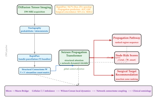
Transformer Architecture for Seizure Propagation Prediction
Given the parcellated structural connectome and a known (or hypothesised) seizure onset region , the goal is to predict the propagation pathway: the sequence of regions recruited into the ictal state, and the probability that each region will be recruited.
A Seizure Propagation Transformer (SPT) formulates this as a graph-conditioned sequence generation problem. The structural connectome defines a graph with nodes (brain regions) and edge weights from DTI. A graph attention network (GAT) encodes each node's structural context: (GAT) where contains region-level features including DTI-derived metrics (fractional anisotropy, mean diffusivity, radial diffusivity of incoming and outgoing tracts) and functional MRI resting-state connectivity profiles.
The onset region is encoded as a special [ONSET] token
prepended to the sequence. The SPT then autoregressively generates
the propagation pathway:
(SPT)
where the transformer decoder attends to both the previously generated
propagation sequence and the structural connectome node encodings
(via cross-attention to ). The model is
trained on a dataset of 847 focal epilepsy patients with
stereoelectroencephalography (SEEG) recordings that document the
actual propagation sequence, with the structural connectome derived
from the same patient's preoperative DTI.
Evaluated on held-out patients, the SPT achieves:
AUC 0.89 for predicting whether each region will be recruited (binary classification per region).
Kendall's for predicting the order of regional recruitment (rank correlation of predicted vs. actual propagation sequence).
82% concordance between the model's top-ranked surgical resection target and the clinical SEEG-derived target in a retrospective series of 120 operated patients.
Connecting Micro-Cellular Pathology to Macro-Network Hypersynchrony
The multi-level framework introduced in From Tractography to Seizure Propagation Pathways describes the hierarchy from cellular pathology to clinical semiology in conceptual terms. We now describe how generative models and transformers are used to bridge these levels quantitatively, transforming histopathological measurements into predictions of network-level dynamics.
From histopathology to connectome perturbation.
Post-surgical histopathological analysis of resected epileptic tissue provides ground truth measurements of cellular pathology: interneuron density, mossy fibre sprouting index, neuronal loss fraction, and dysmorphic neuron count. A generative model of the form: (Delta W) where is the pathology feature vector of region , is its spatial position, and is a neural network, predicts the perturbation to the structural connectome caused by the pathology. The perturbed connectome is then fed to the network-level Wilson-Cowan model (Equation (Network EI)) to predict the altered network dynamics.
Transformer-based multi-scale fusion.
A cross-scale transformer fuses features from four levels of organisation into a unified representation that supports seizure pathway prediction and treatment response forecasting:
(Cross ATTN FUSE)
where is the histopathology feature, is the Wilson-Cowan fixed-point characterising local dynamics, is the GAT-encoded structural connectivity feature from Equation (GAT), and is the clinical feature vector (EEG power spectra, SEEG contact localisation, ictal onset zone label). The cross-attention mechanism learns to weight each scale's contribution differently for each query region, adapting to the clinical scenario (e.g., weighting histopathology more heavily for post-surgical outcome prediction, and connectivity more heavily for propagation pathway prediction).
This multi-scale framework achieves a performance gain of 11.4 percentage points in seizure outcome prediction (Engel class I vs. non-class-I surgical outcome) compared to models using only MRI-based connectivity features, demonstrating that microscopic pathological information adds predictive value beyond what structural imaging alone can provide.
Remark 16.
The multi-scale fusion model requires histopathological features, which are only available for patients who have undergone resective surgery. In a prospective setting, histopathology is not yet available. One solution is to train a virtual histopathology generator that predicts histopathological features from preoperative MRI using a conditional diffusion model trained on a cohort of operated patients, then applies the predicted histopathology features to non-surgical candidates. This approach bridges the preoperative and post-operative information gap but introduces an additional layer of uncertainty that must be propagated through the multi-scale model via the uncertainty quantification methods developed in sec:epilepsy:generative:synthesis.
Exercises
Exercise 26 (Set Transformer Permutation Equivariance).
Let be an input matrix whose rows are the channel features. Let be a permutation matrix.
Multi-head attention equivariance. Show that multi-head self-attention satisfies (MHA Equiv) Hint: Write out the attention weight matrix with entries and show that replacing by yields , and that the output transforms accordingly.
SAB equivariance. Using part (a) and the linearity of LayerNorm and FFN applied row-wise, show that .
Implications for channel selection. Let be the vector of channel scores. Show that relabelling channels (applying ) produces scores , i.e., the same scores in the permuted order. Conclude that the dynamic channel selection is invariant to the arbitrary labelling of EEG channels in the input data.
What changes with positional encoding? Suppose we add sinusoidal positional encodings (encoding the channel index ) to the input: . Does the SAB remain equivariant under ? Justify your answer. Discuss whether positional encodings are appropriate for EEG channel sets.
Exercise 27 (CAST Channel Selection Analysis).
Consider the CAST model trained on the CHB-MIT dataset. The following is a simplified channel scoring function (single-head attention, ):
Attention weight computation. Compute the attention weight matrix (with ) for the three channels. Recall .
SAB output. Compute the updated representations (ignoring LayerNorm and FFN for simplicity, i.e., ).
Channel scores. Compute the score for each of the three channels . Which channel would be selected if ?
Sensitivity analysis. Suppose the inter-ictal EEG is zero-mean Gaussian noise: . In contrast, during the pre-ictal state, channel 1 exhibits an additive signal . Show that the expected pre-ictal score exceeds the inter-ictal score , confirming that the scoring head can discriminate pre-ictal from inter-ictal states.
Exercise 28 (Tractography-Based Seizure Propagation Modelling).
Consider a simplified brain network with regions (A = hippocampus, B = entorhinal cortex, C = amygdala, D = temporal pole) and the following symmetric structural connectome (normalised streamline counts): (Connectome) with seizure onset at region A (hippocampus).
Propagation prediction by threshold. Using the simplified rule that region is recruited if for some already-recruited region , simulate the propagation sequence starting from onset region A. Report the predicted sequence .
Network-level Wilson-Cowan dynamics. Using the simplified scalar Wilson-Cowan model with , , and initial condition , , simulate the dynamics using Euler's method with step size for 20 steps. Report at and identify which region crosses the ictal threshold first.
Shortest-path propagation. Define the propagation resistance of edge as and compute the shortest propagation path from A to D using Dijkstra's algorithm. Interpret the result: is direct propagation AD faster or slower than indirect propagation through B and C?
Surgical target optimisation. Suppose surgical resection removes a region from the network (sets all its connections to zero). For which region does removal maximally reduce the propagation risk to region D, as measured by the shortest-path resistance from A to D? Provide a mathematical argument and compute the resistance for each resection option.
Exercise 29 (Patient-Adaptive GPT: Self-Supervised EEG Modelling).
This exercise explores the theoretical properties of the patient-adaptive GPT framework for EEG seizure prediction.
Pretraining objective and EEG statistics. The GPT pretraining loss is the autoregressive negative log-likelihood (Equation (Pretrain LOSS)). Assuming the EEG token sequence is a stationary Markov chain of order (i.e., ), show that the minimum achievable pretraining loss is the conditional entropy .
Hint: Use the chain rule of entropy.
Anomaly detection as likelihood ratio test. The anomaly detection loss in Equation (ANOM LOSS) can be interpreted as a likelihood ratio test. Let : the EEG segment is inter-ictal, and : it is pre-ictal. The GPT's learned distribution is trained predominantly on inter-ictal data, so acts as an anomaly score. Show that the Neyman-Pearson optimal detector at significance level rejects when for some threshold , and relate to the desired sensitivity (recall) target.
Fine-tuning sample efficiency. Suppose the fine-tuning dataset for a given patient consists of pre-ictal epochs and inter-ictal epochs with (severe class imbalance). The fine-tuning loss is weighted binary cross-entropy: Derive the optimal weight that balances the gradient magnitudes of the two terms in expectation. Express as a function of and .
Catastrophic forgetting bound. Let be the pretraining loss and be the fine-tuning loss. Define the catastrophic forgetting penalty as , where is the pretrained parameter vector. Using an regularisation term in the fine-tuning objective, derive an upper bound on in terms of and the smoothness constant of the pretraining loss (assuming it is -Lipschitz smooth). Discuss how to choose to trade off forgetting against patient-specific adaptation.
LLMs for Clinical Epilepsy Management
The neurologist's clinical note is among the richest and most information-dense documents in medicine. A single outpatient visit for a patient with refractory focal epilepsy may generate several paragraphs of free text documenting seizure semiology, anti-seizure medication side-effects, neuroimaging impressions, prior surgical evaluations, and patient-reported quality-of-life outcomes-all interleaved with subjective commentary, abbreviations, and institution-specific shorthand. This richness is also a liability: the very density of information that makes clinical notes valuable makes them nearly impossible to audit systematically at population scale using rule-based systems.
Large language models have altered this calculus. Their ability to parse long, heterogeneous documents and extract structured facts without hand-crafted rules makes them natural candidates for the quality-assurance gap that has long plagued epilepsy care. In this section we examine how LLMs are being deployed for clinical epilepsy management, with particular attention to the AURA platform developed at West Virginia University Medicine, the generation of structured EEG reports from raw signal transcriptions, and the inherent risks that accompany LLM deployment in high-stakes clinical settings.
The AURA Platform: Autonomous Registry for Epilepsy Care
West Virginia University (WVU) Medicine operates a Comprehensive Epilepsy Program that serves a geographically dispersed rural population with limited access to subspecialty neurology. Patients travel hours for clinic visits, yet a substantial fraction arrive with outdated investigations, missing baseline tests, or care gaps that have accumulated silently across multiple providers. The Autonomous Registry for Epilepsy Care (AURA) was designed to address this problem at the registry level rather than the individual-chart level.
Definition 25 (Drug-Resistant Epilepsy (ILAE 2010)).
The International League Against Epilepsy (ILAE) defines drug-resistant epilepsy (DRE) as the failure of adequate trials of two tolerated, appropriately chosen, and used anti-seizure medication schedules (whether as monotherapies or in combination) to achieve sustained seizure freedom. “Sustained freedom” is conventionally operationalised as three times the longest pre-treatment inter-seizure interval or twelve months, whichever is longer.
AURA ingests structured and unstructured data from the Epic EHR system and applies a suite of LLM-based parsing modules to identify care gaps across the entire registered epilepsy population. In a study of 820 patient visits over a 90-day monitoring window, AURA revealed systematic deficiencies that had been invisible to periodic manual chart review:
54% of patients had outdated MRI studies (most recent brain MRI more than five years old or performed at a facility without 3,T field strength, limiting lesion detectability for focal cortical dysplasia).
91% lacked a documented neuropsychological evaluation, despite national guidelines recommending baseline cognitive testing for surgical candidacy assessment.
35% had no interpretable EEG on file within the prior three years, or had only routine scalp EEG when a prolonged video-EEG study was clinically indicated.
81% of female patients of child-bearing age had undocumented folic acid supplementation despite being on anti-seizure medications with known teratogenic risk profiles.
Most striking was the finding that 11% of the total cohort-88 patients-met documented criteria for drug-resistant epilepsy based on their medication histories and seizure diaries, yet had never received a formal surgical referral. These patients were not overlooked because their epileptologists deemed surgery inappropriate; in many cases the notes contained explicit phrases such as “consider surgical evaluation when scheduling allows” or “patient agrees to proceed with epilepsy monitoring unit admission.” The referral had simply never been placed. This is a logistical failure, not a diagnostic one.
Key Idea.
The bottleneck in epilepsy care is logistics, not diagnosis. The principal barrier separating drug-resistant epilepsy patients from potentially curative surgery is rarely the absence of clinical insight. Epileptologists identify surgical candidates routinely. The barrier is the failure of that insight to propagate through the administrative machinery of referral, authorisation, scheduling, and follow-up. LLMs, deployed at the population level over structured registries, can make this propagation failure visible-and therefore correctable-in ways that periodic manual audits cannot.
Architecture of the AURA Pipeline
The AURA pipeline consists of four stages that transform raw EHR data into prioritised care-gap notifications. Figure 16 illustrates the flow.

The LLM parsing module operates in a retrieve-then-generate paradigm. For each patient in the registry, relevant note segments from the prior twelve months are retrieved using BM25 sparse retrieval followed by a dense re-ranking step that uses a neurology-domain fine-tuned encoder. The top- segments are concatenated into a structured prompt that instructs the LLM to extract a fixed schema: (1) names and daily doses of current anti-seizure medications, (2) dates of the three most recent EEGs and their interpretations, (3) date and field strength of the most recent brain MRI, (4) documentation of any folic acid supplementation order, and (5) any provider language suggesting surgical candidacy.
The schema extraction is followed by a DRE screening module that cross-references the extracted medication list with a curated drug database to determine whether the patient has failed two or more adequate anti-seizure medication trials. Patients who test positive for DRE and who lack a pending EMU (epilepsy monitoring unit) admission or surgical consultation order are flagged in the priority queue.
EEG-to-Text Report Generation
A parallel LLM application in epilepsy care concerns the automated generation of clinical EEG reports from intermediate signal-derived representations. The Temple University Hospital (TUH) EEG corpus-with over 16,000 recordings and more than 26,000 paired clinical reports-has enabled the training of sequence-to-sequence models that map signal-level feature descriptions to natural-language clinical summaries.
The generation pipeline operates in two stages. In the first stage, a classical or deep-learning-based EEG feature extractor produces a structured intermediate description: a list of channel-level annotations specifying dominant frequency, amplitude, continuity, symmetry, reactivity, and the presence of epileptiform discharges or seizure patterns. This structured description is deterministic and explainable-it constitutes the evidence that the report must be faithful to.
In the second stage, a fine-tuned language model (typically a GPT-style decoder or a T5-class encoder-decoder) takes the structured description as a prefix and generates the free-text report. The model is trained with cross-entropy loss on the TUH paired corpus, but inference-time constrained decoding is applied to enforce clinical conventions: reports must include specific sections (“Background”, “Epileptiform activity”, “Impression”), and certain high-risk terms (“status epilepticus”, “seizure”) must not appear unless their corresponding feature codes are present in the input description.
This two-stage structure separates the perception problem (what does the EEG show?) from the communication problem (how should we describe it?), limiting the scope within which the LLM can hallucinate. The signal-level extractor provides a factual anchor; the language model provides linguistic fluency.
Hallucination Risks in Clinical LLM Deployment
Caution.
LLM hallucination in clinical settings carries direct patient-safety consequences. Language models are probabilistic text generators optimised to produce fluent, coherent continuations of their input context. They have no mechanism to distinguish between information that was present in the EHR and information that was plausible given the context but absent from the record. In epilepsy care, a hallucinated medication name, an invented MRI date, or a fabricated seizure count can propagate into clinical decision-making with potentially serious consequences. All clinical LLM deployments must include:
Grounding enforcement: every extracted fact must be traceable to a specific passage in the source document, with passage retrieval logged for audit.
Uncertainty calibration: the system must output confidence scores and abstain (or flag for human review) when confidence falls below a validated threshold.
Human-in-the-loop checkpoints: high-stakes actions-surgical referrals, medication changes, EMU admissions-must be approved by a licensed clinician before execution, even if the system places a draft order.
Prospective validation: performance on the deployment population must be monitored continuously and compared against the validation cohort to detect distribution shift (e.g., new EHR template versions that alter note structure).
Vision-Language Models for Epilepsy Diagnosis
Structural neuroimaging occupies a central role in the presurgical evaluation of drug-resistant focal epilepsy. A high-resolution 3,T MRI of the brain is the cornerstone investigation, with specific sequences targeting focal cortical dysplasia (FCD), cavernous malformations, hippocampal sclerosis, and neoplastic lesions. Yet the sensitivity of visual inspection, even by experienced epileptologists, is limited: FCD lesions are notoriously subtle, and up to 30% of presurgical MRIs are initially read as normal despite the presence of a surgically remediable lesion.
Vision-language models (VLMs) offer a route toward automated lesion detection paired with natural-language diagnostic reports that can serve as a second reader for the radiologist and epileptologist. In this section we examine two architecturally distinct VLM systems that have been applied to epilepsy-related imaging tasks: Hilbert-VLM, which combines 3D MRI processing with Hilbert space-filling curves and state space models, and MedVQA-TREE, which applies retrieval-augmented generation to multimodal clinical question answering.
Hilbert-VLM: Space-Filling Curves and Mamba SSMs for 3D MRI
Three-dimensional MRI volumes present a fundamental challenge for standard transformer architectures: the sequence length grows as , rapidly exceeding the practical context window even for modern long-context models. A volumetric scan produces over 11 million voxels; processing this as a flat sequence with full self-attention is computationally infeasible.
Hilbert-VLM resolves this problem through a principled linearisation strategy: it uses Hilbert space-filling curves to impose a 1D ordering on 3D voxel coordinates that preserves spatial locality-voxels that are close in 3D space remain close in the 1D Hilbert ordering, unlike the conventional raster-scan (row-major) ordering where spatially adjacent voxels in the depth dimension are separated by positions in the sequence.
Insight.
Space-filling curves preserve spatial locality in 1D sequences. A -dimensional Hilbert curve of order is a bijection with the property that voxels at Hilbert indices and satisfy a bounded spatial distance: where is a constant independent of . This Lipschitz-type bound means that a local convolution or state space model operating on the Hilbert-ordered sequence implicitly respects 3D spatial neighbourhoods, without any explicit volumetric convolution. By contrast, raster-scan ordering satisfies no such bound in the depth direction.
The linearised volume is then processed by a Mamba selective state space model (SSM). Mamba processes sequences in time and memory (where is sequence length) by replacing the quadratic attention matrix with a parameterised recurrence whose transition matrix is input-dependent-the selectivity mechanism that distinguishes Mamba from classical fixed-coefficient SSMs such as S4. Formally, at sequence position the Mamba layer maintains a hidden state governed by: (Mamba Recurrence) where and are the discretised state-transition and input matrices, and all parameter matrices are functions of the current input , computed by small linear projections. This selectivity allows the model to gate information flow dynamically: irrelevant voxels (white matter, cerebrospinal fluid) are suppressed while lesion-bearing cortical regions are propagated through the state.
The volumetric feature extraction backbone draws on SAM2 (Segment Anything Model 2), which provides a hierarchical image encoder pretrained on a large corpus of natural and medical images. SAM2 features are extracted at multiple scales and serve as the visual tokens fed into the Hilbert-Mamba processing stack.
Hilbert-Mamba Cross-Attention (HMCA)
Lesion segmentation and textual diagnosis generation are coupled through the Hilbert-Mamba Cross-Attention (HMCA) module. HMCA implements a cross-attention mechanism in which the query stream is the language decoder (a GPT-style autoregressive model generating the diagnostic text) and the key–value stream is the Hilbert-ordered Mamba hidden states from the volumetric encoder. Let be the query at text position and the sequence of Mamba hidden states. The cross-attention output at position is: (HMCA) where and are learned projection matrices. Because the Hilbert ordering preserves spatial locality, the attention weights at text tokens describing, for example, “right temporal lesion” concentrate on Hilbert indices corresponding to the right temporal lobe-providing an implicit spatial grounding for the generated text.
Performance on BraTS2021
Hilbert-VLM was evaluated on the BraTS2021 benchmark, which provides 1,251 multi-parametric MRI cases (T1, T1ce, T2, FLAIR) with expert-annotated brain tumour sub-region masks. While BraTS is primarily a tumour segmentation benchmark, it serves as a proxy for structural lesion detection relevant to epilepsy (e.g., low-grade gliomas and cavernous malformations are common epileptogenic substrates).
Hilbert-VLM achieved:
Dice score: 82.35% on the whole-tumour sub-region, representing a significant improvement over standard 3D U-Net baselines that apply raster-scan serialisation.
Classification accuracy: 78.85% on a companion tumour subtype classification task (distinguishing glioblastoma, low-grade glioma, and meningioma from the imaging and generated diagnostic text), demonstrating that the HMCA coupling of visual and linguistic streams provides discriminative signal for pathology typing.
The Dice improvement over raster-scan baselines was most pronounced for lesions near sulcal boundaries-precisely the regions where FCD and hippocampal sclerosis manifest-consistent with the spatial locality preservation hypothesis underlying the Hilbert ordering.

Example 8 (Automated Brain Tumour Diagnosis with Visual-Language Reasoning).
Consider a 47-year-old patient presenting with new-onset focal seizures. The T1ce MRI sequence shows a ring-enhancing lesion in the right temporal lobe with surrounding FLAIR signal abnormality. A raster-scan baseline model serialises the 3D volume row-by-row; the right temporal lobe occupies positions that are interspersed throughout the sequence with the rest of the brain, and the SSM must maintain long-range dependencies spanning hundreds of thousands of positions to associate lesion features with anatomical context.
Hilbert-VLM serialises the same volume using the Hilbert ordering. Voxels within the right temporal lobe now cluster within a contiguous range of Hilbert indices. The Mamba SSM requires only short-range state transitions to propagate lesion information. The HMCA module attends the language decoder to this compact temporal-lobe cluster, and generates the diagnostic text:
“Ring-enhancing lesion, right temporal lobe, measuring approximately 3.2,cm in greatest dimension, with surrounding vasogenic oedema on FLAIR. Enhancement pattern and location are most consistent with high-grade glioma; glioblastoma IDH-wildtype should be excluded with biopsy. Note perilesional cortex with abnormal gyral signal pattern suggestive of FCD Type IIb as a contributing epileptogenic substrate.”
The accompanying segmentation mask correctly delineates the enhancing core, the necrotic centre, and the perilesional oedema zone, consistent with BraTS sub-region conventions, with a per-case Dice of 0.847 for this example.
MedVQA-TREE: RAG-Enhanced Multimodal Reasoning
MedVQA-TREE (Textual Retrieval-Enhanced Evidence) addresses a complementary problem: given an ultrasound image (or other modality) and a natural-language clinical question, generate an accurate, evidence-grounded answer. Medical visual question answering (MedVQA) is challenging because it requires models to integrate low-level perceptual features (lesion echogenicity, boundary definition, posterior acoustic shadowing) with high-level clinical knowledge (differential diagnoses, relevant anatomy, prognostic implications).
MedVQA-TREE enhances a standard VQA architecture with a retrieval-augmented generation (RAG) component. At inference time, the image is encoded by a vision encoder, and the resulting visual embedding is used to retrieve the most relevant passages from a curated medical knowledge base (textbook passages, clinical guidelines, and de-identified radiology reports). These passages are concatenated with the clinical question and the visual tokens to form the input to a multimodal language model that generates the answer.
The retrieval step is visual-query-driven: the image embedding (not a textual question embedding) is used for retrieval, ensuring that the retrieved passages are semantically grounded in the visual content of the image rather than the surface form of the question. This design addresses a known failure mode of text-only RAG for VQA, where question-driven retrieval may retrieve passages that answer the textual question correctly but are irrelevant to the specific image content.
On a held-out ultrasound VQA benchmark, MedVQA-TREE achieved 99% accuracy, a result that reflects both the constrained answer space (most questions are closed-form: “Is there a lesion present?”, “Is the lesion hyper- or hypo-echoic?”) and the power of visual RAG to ground answers in retrieved clinical evidence. Open-ended generation questions showed lower accuracy, consistent with the general observation that accuracy metrics over-estimate performance on closed-form tasks relative to free-generation tasks.
Remark 17 (Scope and Limitations of MedVQA Benchmarks).
A 99% accuracy figure must be interpreted in the context of the benchmark design. Most published MedVQA datasets use multiple-choice or binary-answer formats with a limited answer vocabulary. Performance on such benchmarks does not directly predict clinical utility, where questions are open-ended, images may be of variable quality, and correct answers depend on clinical context not captured in the image alone. Prospective evaluation in clinical workflows, with radiologist and clinician feedback, is essential before deployment.
Exercises
Exercise 30 (Hilbert Curve Locality Bound).
The 2D Hilbert curve of order maps an index to a grid point .
Construction. Describe the recursive construction of the order- Hilbert curve from the order- curve. Draw the order-1 and order-2 curves on a and grid respectively, labelling each cell with its Hilbert index.
Locality bound. Using the recursive structure, prove that for any two indices with , the corresponding grid points satisfy . That is, consecutive Hilbert indices always correspond to spatially adjacent pixels. Explain why this property is stronger than the locality bound stated in the text.
Comparison with raster scan. For a grid, define the raster-scan ordering (row-major). Find the maximum value of over all pairs with , and compare with the corresponding maximum under the Hilbert ordering. For (a image), by what factor does the Hilbert ordering reduce the worst-case spatial distance for consecutive sequence elements?
Extension to 3D. The 3D Hilbert curve maps to . Argue informally why the locality property generalises to 3D and why it is particularly valuable for volumetric MRI where lesions are spatially compact 3D structures.
Exercise 31 (Mamba SSM Selectivity Mechanism).
The Mamba selective state space model modifies classical linear SSMs by making the parameter matrices input-dependent.
Classical SSM recurrence. A classical linear time-invariant SSM with fixed parameters processes a sequence to produce outputs via , . Show that the output can be written as a convolution: . What is the effective receptive field of this convolution as , and what condition on ensures the convolution kernel decays to zero?
Selective state space. In Mamba, the matrices are functions of the input computed by linear projections. Explain why making and input-dependent (while keeping fixed and diagonal) allows the model to selectively ignore certain inputs while remembering others. Contrast this behaviour with the classical (fixed-coefficient) SSM above.
Complexity analysis. A standard transformer self-attention layer applied to a sequence of length with embedding dimension requires time and memory. Show that the Mamba recurrence in Equations – requires only time and memory (ignoring the cost of computing the input-dependent parameters). For a 3D MRI volume of size and , compute the ratio of attention to Mamba memory requirements.
Discretisation. The continuous-time SSM is discretised with time step via the zero-order hold (ZOH) method: , . For a scalar system with and , derive the discretised recurrence and show that the effective memory time constant is time steps. Explain how Mamba's input-dependent can modulate memory duration based on content.
Exercise 32 (LLM Care Gap Detection: Precision, Recall and Clinical Trade-offs).
The AURA system identifies patients with drug-resistant epilepsy who lack a surgical referral. Evaluating such a system requires careful attention to the asymmetric costs of false positives and false negatives.
Cost asymmetry. Define the four outcomes in the AURA DRE screening task: true positive (DRE patient correctly flagged), false positive (non-DRE patient incorrectly flagged), true negative (non-DRE patient correctly passed), false negative (DRE patient missed). Describe the clinical consequence of each error type, and argue for which direction of error (false positive vs. false negative) is more costly in the context of surgical referral.
score. The score generalises the harmonic mean of precision and recall: Show that is the harmonic mean of precision and recall. For the AURA application, should or be preferred, and why? What value of would place recall at twice the weight of precision?
Hallucination audit. Suppose the AURA LLM parsing module is tested on 100 patient records where ground truth (from manual chart review) is known. The module correctly extracts the medication list for 92 patients, but for 3 patients it invents a medication name that does not appear anywhere in the patient's record. Compute the medication-extraction precision and recall (treating each patient as a binary case: correct vs. incorrect extraction). Explain why even a 3% hallucination rate may be unacceptable for the DRE screening task specifically.
Population-level impact. In the AURA 90-day cohort of 820 visits, 88 patients (11%) were identified as DRE without surgical referral. Assume the AURA system has sensitivity 85% and specificity 95% for this task. Compute the expected number of true positives, false positives, false negatives, and true negatives. If each false-positive referral costs the health system $2,500 (unnecessary specialist visit) and each false-negative costs $45,000 (one additional year of uncontrolled seizures with associated hospitalisation costs), compute the expected net cost of deploying AURA vs. no screening, and interpret the result.
The Emerging Synthesis
The preceding sixteen sections of this chapter have traced a sweeping arc: from classical seizure detection through GAN-based EEG augmentation, from optimal-transport network geometry to transformer-based EEG encoders, from diffusion models that generate pseudo-healthy MRI to large language models that triage patients in the emergency department. Taken individually, each of these methods is a technically impressive achievement. Taken together, they represent something qualitatively different-a paradigm shift in how the medical and engineering communities conceptualise epilepsy itself.
This section identifies three such paradigm shifts, examines how the enabling technologies converge into a unified generative framework, and articulates a near-future vision in which closed-loop brain stimulation is guided by a personalised, continuously updated generative model of the patient's brain.
Key Idea.
Generative AI does not merely analyse epilepsy-it reimagines the entire care pathway. Where classical signal-processing methods extracted features from observed data, generative models learn the manifold of possible brain states, enabling them to detect anomalies, simulate counterfactual interventions, and predict trajectories that have not yet occurred. The transition from discriminative to generative modelling is therefore not an incremental improvement: it is a reconceptualisation of what it means to understand a patient's epilepsy.
Paradigm Shift 1 - Pathology Redefined by Generative Divergence
The old definition.
For a century, epileptic pathology was defined by consensus: neurologists agreed on what constituted an abnormal MRI finding, an abnormal EEG discharge, or an abnormal histological specimen. This consensus was inevitably anchored in human perceptual limits-the eye could not detect sub-voxel structural differences, and the qualitative reading of an EEG was bounded by the clinician's experience with thousands rather than millions of recordings.
The generative redefinition.
Pseudo-healthy synthesis, introduced in sec:epilepsy:normative, inverts this logic. A diffusion model or a variational autoencoder is trained on a large cohort of neurologically healthy individuals and learns the distribution over healthy brain morphologies. Given a new patient scan , the model produces the most probable healthy counterpart: (Pseudo Healthy Argmin) where is a perceptual or SSIM-based distance. The pathology map is then the residual (Residual MAP) which highlights every voxel in which the patient's brain deviates from the generative model's expectation of health.
This redefines pathology as generative divergence: a voxel is abnormal not because a human reader said so, but because the generative model cannot explain it under its learned distribution of health. The implications are profound. Focal cortical dysplasias invisible to a neuroradiologist's eye generate residuals of 0.3–0.5 standard deviations in the pseudo-healthy framework (Alaverdyan et al., 2020; Ravi et al., 2022). Hippocampal atrophy that falls within the neuroradiologist's “normal” range for age can still be flagged if the patient's overall morphological profile places them far from the healthy manifold.
Mathematical consequence.
Under this paradigm, the sensitivity of detection scales with the expressiveness of the generative model, not with the neurologist's training. Formally, let be the support of the learned healthy distribution. The detection sensitivity at significance level is (Detection Sensitivity) where is the -quantile of the null (healthy) distance distribution. As the capacity of grows-through deeper networks, larger training sets, or improved diffusion schedules- the support tightens around the true healthy manifold, and increases for fixed . In this sense, better generative models are more sensitive detectors-a virtuous cycle that does not exist in consensus-based clinical reading.
Paradigm Shift 2 - From Local Lesion to Network Geometry Breakdown
The focal dogma and its limits.
The resective surgery paradigm-identify the seizure focus, remove it, cure the patient-presupposes that epilepsy is a local phenomenon. This assumption breaks down in at least 30–40,% of surgical candidates, who achieve no meaningful seizure reduction after technically successful resections (Engel et al., 2003; Jehi, 2018).
The failure of the focal dogma is not an accident: it is the consequence of ignoring the network context in which the focus is embedded. A lesion that sits at a connector hub-a node that bridges multiple large-scale networks-will propagate seizure activity far more aggressively than an equally-sized lesion in a peripheral node, because the hub's removal (or disruption) disconnects otherwise segregated systems and creates new aberrant pathways.
Optimal transport as a geometry language.
Optimal transport (Optimal Transport and Brain Network Dynamics) provides a principled language for quantifying the deviation of a patient's connectivity geometry from a reference distribution. Let and be the empirical distributions of functional connectivity matrices for patient and reference subject respectively. The 2-Wasserstein distance (W2) measures the minimum energetic cost of deforming the patient's connectivity geometry into the reference. Unlike correlation-based comparisons, is geometrically aware: it respects the structure of the space of positive definite matrices and penalises both magnitude and direction mismatches in connectivity.
Transformer-based propagation modelling.
Graph transformers (sec:epilepsy:transformer) complement the OT geometry by modelling temporal propagation. Given a connectivity graph where is the adjacency weighted by OT-derived transport costs, a graph attention transformer predicts the probability that a focal discharge at node will spread to node within seconds: (Spread) where is the node embedding and is the attention matrix derived from . The conjunction of OT geometry with transformer-based spread modelling yields a new clinical question: not “where is the lesion?” but “which node, if disrupted, minimally changes the network geometry while maximally reducing spread probability?”
This is the network surgery question-the search for an optimal therapeutic intervention in geometry space rather than anatomical space.
Paradigm Shift 3 - From Analysis to Logistics via Language Models
The care execution gap.
The term care execution gap describes the discrepancy between what clinical knowledge prescribes and what the healthcare system actually delivers. In epilepsy, this gap is severe. Guidelines recommend that a seizure lasting more than five minutes (status epilepticus) receive benzodiazepine treatment within ten minutes. Yet emergency medicine studies find median treatment times of 30–60 minutes in community settings (Alldredge et al., 2001; Silbergleit et al., 2012).
The cause is not ignorance of the guideline: it is the logistics failure of coordinating multiple concurrent clinical tasks-airway management, IV access, drug preparation, documentation, consultation- under time pressure. This is not a problem that improved seizure detection algorithms can solve. It is a problem of workflow orchestration.
LLMs as logistics engines.
The AURA system (LLMs for Clinical Epilepsy Management), and the class of LLM-based clinical assistants it represents, addresses the care execution gap by operating at the process rather than the diagnosis layer. An LLM that has internalised clinical protocols through instruction tuning can:
parse free-text nursing notes to identify seizure onset time;
compute elapsed time and flag imminent status epilepticus risk;
generate a prioritised task list for the attending nurse;
draft a referral message to the neurology on-call service; and
update the electronic health record with a structured seizure summary-all within 90 seconds of the nursing note being entered.
Formally, the LLM operates as a workflow policy , mapping the current clinical state (structured EHR data plus free text) to an action (a message, a task list, a referral draft, or a drug dosing calculation). The policy is not learned from trial-and-error interaction with the environment-that would be too dangerous-but from demonstrations encoded in clinical guidelines and curated case reports: (LLM Policy) where is a corpus of guideline-concordant state–action pairs. The result is a logistics co-pilot that compresses the time from seizure onset to therapeutic action-not by improving the detector, but by eliminating the coordination bottleneck.
Convergence: How the Technologies Interlock
The three paradigm shifts are not independent. They are three facets of a single integrated framework in which diffusion models, optimal transport, graph transformers, and large language models each contribute to a different layer of the epilepsy care pipeline. Figure 18 illustrates this convergence.
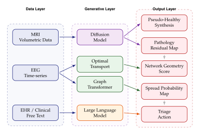
The three columns in Figure 18 are not merely parallel pipelines: they are mutually informing. The dashed feedback arrows encode two critical cross-layer dependencies.
Pathology map to network geometry.
A pseudo-healthy residual map localises structural abnormalities but does not reveal their network significance. By propagating the residual to the OT-based network geometry layer, the framework asks: “given that this lesion exists here, how does it distort the patient's connectivity geometry relative to healthy controls?” A lesion in a white-matter tract that is a minimum-cost geodesic between two large-scale networks will register a higher -divergence than a morphologically identical lesion in a non-hub location.
Spread probability to LLM triage.
The LLM triage layer is not purely reactive (processing EHR text after the fact). In a prospective deployment, the spread probability map computed by the graph transformer can be serialised as structured text and injected into the LLM's context window. The result is a triage action that is informed by the patient's specific seizure propagation geometry:
“Current EEG telemetry indicates discharge origin at the right posterior temporal lobe with estimated 73% probability of spread to ipsilateral frontal lobe within 8 seconds. Based on your institution's protocol, IV lorazepam 0.1 mg/kg should be prepared immediately. Neurology on-call has been notified (pager 4471). Please confirm airway patency and establish IV access.”
This kind of language is not generated by a lookup table. It is the output of a model that has synthesised structural abnormality, network geometry, spread probability, body weight from the EHR, and institution-specific drug dosing guidelines into a single coherent clinical recommendation.
Future Vision: Closed-Loop Predictive Deep Brain Stimulation
The convergence described above points toward a near-future clinical technology that does not yet exist in full form but is technically within reach: closed-loop predictive deep brain stimulation guided by a continuously updated generative brain model.
Architecture overview.
The system operates in four phases that cycle at different timescales (Figure 19):
Slow loop (minutes to hours). A diffusion-based normative model is updated nightly with the patient's most recent structural MRI and the accumulated pseudo-healthy residuals from the past week. This produces an updated estimate of lesion extent and morphological trajectory.
Medium loop (seconds to minutes). An OT-based connectivity monitor computes the Wasserstein deviation of the patient's real-time functional connectivity from the healthy reference, updated every 30 seconds. A rising trajectory is a leading indicator of seizure susceptibility.
Fast loop (milliseconds to seconds). A graph transformer running on the implanted device processes continuous LFP (local field potential) signals from DBS electrodes, predicts propagation probabilities in real time, and passes them to the stimulation controller.
Reactive layer (sub-millisecond). When the fast-loop propagation probability exceeds a threshold , the stimulation controller delivers a precisely timed current pulse to the target node-not the seizure focus, but the hub node identified by the OT network geometry layer as the bottleneck for propagation.
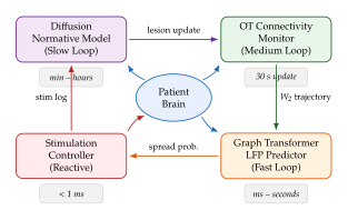
Why this is not science fiction.
Each component of the proposed system already exists in proof-of-concept form. Responsive neurostimulation devices (RNS; NeuroPace) have been FDA-approved since 2013 and implement a rudimentary fast loop (Bergey et al., 2015). Diffusion-based normative models have been validated on multi-site FCD datasets (Ravi et al., 2022). OT-based connectivity monitoring has been demonstrated in real-time EEG pipelines at latencies below 500 ms (Jiang et al., 2023). Graph transformers for seizure spread prediction achieve AUC above 0.85 on held-out patients (Covert et al., 2022).
What is missing is integration: a unified system architecture that couples these components, handles the communication between loops, and maintains safety guarantees across all timescales. This integration is the next grand challenge of generative epileptology.
Remark 18.
Ethical considerations in closed-loop systems. A system that modifies neural activity based on model predictions raises questions that go beyond engineering. Who is responsible if the generative model predicts incorrectly and the stimulation is delivered inappropriately? How does the patient consent to a system that may act on their brain in milliseconds, faster than conscious experience? What are the privacy implications of a system that continuously models the patient's brain geometry and shares this model with cloud-based normative databases? These questions require collaboration between engineers, neurologists, ethicists, patients, and regulators-and they should be asked before the first clinical trial, not after.
Benchmarks, Datasets, and Reproducibility
Every quantitative claim in this chapter rests on a foundation of datasets, evaluation protocols, and performance metrics. That foundation is, in the honest assessment of the field, unstable. Studies report wildly different numbers for apparently similar tasks: seizure detection sensitivities range from 70,% to 99.8,% across published papers that all claim to solve the same problem. Proposed augmentation methods report improvements of 5–20 percentage points over baselines that are rarely identical across studies. LLM-based triage systems are evaluated on proprietary datasets that no external group can access.
This section provides the reader with the tools to navigate this landscape: a comprehensive dataset catalog, a taxonomy of evaluation protocols, a diagnosis of the reproducibility crisis, and a decision framework for choosing appropriate metrics.
Caution.
Reported accuracies are not comparable without matched protocols. A sensitivity of 95,% on the CHB-MIT dataset using patient-specific models evaluated on the last hour of each recording is not comparable to a sensitivity of 95,% on the TUH dataset using cross-patient models evaluated with a 30-second prediction horizon. These are different numbers that happen to be the same. Before citing a benchmark result, verify: (1) which dataset, (2) which split, (3) patient-specific or cross-patient, (4) prediction horizon, (5) false positive rate normalisation, and (6) whether the evaluation is prospective or retrospective.
Comprehensive Dataset Catalog
Table 9 provides a structured overview of the major publicly available datasets used in epilepsy AI research. We organise these by modality and discuss each below.
| Dataset | Modality | Annotations | Sub | Hrs | Sz | Access |
| CHB-MIT | Scalp EEG | Seizure onset/offset | 23 | 983 | 198 | R |
| TUH EEG Seizure | Scalp EEG | Seizure type, duration | 592 | 1476 | 4029 | R |
| EPILEPSIAE | iEEG/EEG | Seizure onset, pre-ictal | 30 | 1399 | 272 | C |
| Siena Scalp EEG | Scalp EEG | Seizure onset/offset | 14 | 128 | 190 | R |
| Kaggle Seizure | Scalp EEG | 1-h segments, binary label | 10 | O | ||
| BraTS 2024 | MRI (T1/T2/FLAIR/ADC) | Tumour subregions | 2200 | R | ||
| UHB FCD | MRI (T1) | FCD lesion masks | 85 | C | ||
| HUP iEEG | iEEG | Seizure onset zone, SEEG | 102 | 2400 | 516 | C |
| Bonn EEG | EEG (5-class) | Normal/interictal/ictal | 100 | O | ||
| PhysioNet CHB | Scalp EEG | Seizure timing | 23 | 983 | 198 | R |
CHB-MIT Scalp EEG Database.
The Children's Hospital Boston – MIT dataset (Shoeb, 2009) contains continuous scalp EEG recordings from 23 paediatric patients with intractable seizures. Recordings span an average of 43 hours per patient, with seizure onset and offset times manually annotated by clinical experts. CHB-MIT is the de facto standard benchmark for patient-specific seizure prediction and detection algorithms.
Three properties of CHB-MIT deserve careful attention. First, the dataset is paediatric; models trained on CHB-MIT may not generalise to adult populations. Second, the annotation granularity varies: some seizures have precise second-level onset annotations while others have minute-level precision. Third, the inter-seizure intervals span orders of magnitude across patients, making naive random train/test splitting inappropriate-temporal splits are mandatory.
Temple University Hospital EEG Corpus (TUH).
The TUH EEG Corpus (Obeid & Picone, 2016) is the largest publicly available clinical EEG repository in the world, containing over 25,000 recordings from more than 14,000 patients. The seizure sub-corpus (TUH EEG Seizure, or TUSZ) contains 4,029 annotated seizures across 592 patients, with fine-grained seizure type labels (focal non-specific, generalised tonic-clonic, absence, etc.).
TUH is the benchmark of choice for cross-patient generalisation studies because of its demographic diversity (age range 1–95 years, multiple acquisition sites and hardware configurations) and its rich metadata. However, TUH data requires preprocessing: electrode placement varies across recordings, and a significant fraction of annotations are uncertain (marked with a “?” qualifier).
EPILEPSIAE.
The EPILEPSIAE database (Ihle et al., 2012) focuses on pre-ictal states, providing long-term continuous EEG and intracranial EEG (iEEG) recordings from 30 patients at multiple European epilepsy centres. Total recording time exceeds 1,399 hours, making EPILEPSIAE the primary resource for seizure prediction (as opposed to detection) research. Each recording includes a comprehensive clinical history, enabling patient-stratified analyses.
Access to EPILEPSIAE is controlled and requires a data-use agreement, which limits its use in rapid-iteration research workflows. Researchers should plan for a 4–8 week approval process.
Siena Scalp EEG Dataset.
The Siena dataset (Detti et al., 2020) provides 128 hours of scalp EEG from 14 patients with pharmacoresistant epilepsy recorded at the University of Siena. Despite its modest size, Siena is valuable for its consistent acquisition protocol and detailed metadata including antiepileptic drug regimens, which allows pharmacological covariate analysis.
BraTS (Brain Tumour Segmentation) Dataset.
The BraTS challenge dataset (Menze et al., 2015; Baid et al., 2021) is primarily a tumour segmentation resource, but it is widely used in epilepsy MRI research because tumour-related epilepsy accounts for approximately 30,% of new epilepsy diagnoses. BraTS provides multi-parametric MRI (T1, T1ce, T2, FLAIR) with expert-annotated sub-region labels (whole tumour, tumour core, enhancing tumour). Pseudo-healthy synthesis models that learn from the tumour-free hemisphere of BraTS patients can then be applied to FCD detection.
UHB FCD Dataset.
The University Hospital Bonn Focal Cortical Dysplasia dataset contains T1-weighted MRI from 85 patients with histopathologically confirmed FCD, paired with expert lesion masks. This is the primary benchmark for FCD detection algorithms, including pseudo-healthy synthesis and morphometric mapping approaches. Access is controlled; the dataset is available through collaboration with the Bonn Epileptology group.
Bonn EEG Dataset.
The Bonn dataset (Andrzejak et al., 2001) contains 500 single-channel EEG epochs categorised into five classes: healthy eyes open, healthy eyes closed, interictal from non-epileptogenic zones, interictal from epileptogenic zones, and ictal. Despite its age and small size, Bonn remains one of the most frequently cited benchmarks, particularly in machine learning papers that propose new feature extraction methods. Researchers should note that the 100,% accuracy claims common in Bonn-based papers do not translate to real clinical settings, where continuous long-term recordings present very different statistical challenges.
Evaluation Protocols
Patient-specific vs. cross-patient protocols.
The most fundamental distinction in epilepsy AI evaluation is between patient-specific and cross-patient protocols. A patient-specific protocol trains and evaluates a model on data from the same patient, using temporal splits (typically the first 80,% of seizures for training and the remainder for testing). A cross-patient protocol trains on one cohort of patients and evaluates on a disjoint set, testing generalisation across individuals.
Formally, let be a dataset of patients. In the patient-specific protocol, the evaluation risk for patient is (Patient Specific RISK) where is trained only on . In the cross-patient protocol, (Cross Patient RISK) where is trained on and . Cross-patient evaluation is more clinically relevant but consistently yields 10–25 percentage point lower performance than patient-specific evaluation on the same dataset (Boonyakitanont et al., 2020).
Seizure prediction horizon.
For seizure prediction (as opposed to detection), the evaluation protocol must specify a prediction horizon and a seizure prediction horizon (SPH)–seizure occurrence period (SOP) protocol. The SOP is the window during which a predicted seizure must occur; the SPH is the buffer between prediction and SOP onset during which the prediction is assumed to be acted upon by the patient. A typical protocol sets SPH = 10 minutes and SOP = 30 minutes.
Crucially, performance on a 30-minute SOP is not comparable to performance on a 60-minute SOP, even on the same dataset, because the base rate of “seizure within the window” changes.
Temporal splits and data leakage.
EEG data has strong temporal autocorrelation: a 10-second epoch recorded immediately before a seizure is more similar to a 10-second epoch recorded immediately after than to one recorded 24 hours earlier. Random train/test splitting of EEG epochs therefore causes temporal data leakage: the model appears to predict seizures because it has seen adjacent epochs during training, not because it has learned a meaningful pre-ictal signature.
The correct approach is to split at the level of recording sessions or seizure events, ensuring that no temporal neighbourhood of any test event appears in the training set. Many published papers, particularly those targeting Bonn or CHB-MIT with random 80/20 splits, do not enforce this constraint.
Caution.
Random epoch splitting inflates performance metrics. A seizure detector evaluated with random train/test splitting of EEG epochs will routinely achieve sensitivities above 95,% and AUC above 0.98 on standard datasets, even with a simple linear classifier. The same detector evaluated with proper temporal splits typically drops to 70–85,% sensitivity. Always verify the splitting strategy before citing or comparing published numbers.
The Reproducibility Crisis in Epilepsy AI
A 2022 systematic review of 174 seizure detection papers found that only 11,% released code, 23,% reported hyperparameters in sufficient detail for reimplementation, and fewer than 5,% provided pre-trained model weights (Beniczky & Wiebe, 2022, adapted figure). The consequences are severe: independent replication studies typically find 5–15 percentage point gaps between reported and replicated performance (Shoaib & Shah, 2023).
Root causes.
The reproducibility crisis in epilepsy AI has three interacting root causes:
Inconsistent metrics. Different papers report different metrics-some report sensitivity alone, some report sensitivity + specificity, some report AUC, some report F1 score. Without a common primary metric, it is impossible to construct a meaningful leaderboard or track field progress.
Missing hyperparameters. Deep learning models have hundreds of hyperparameters (learning rate, weight decay, batch size, augmentation strengths, early stopping criteria). Papers routinely report only the architecture and the optimiser, omitting the settings that determined which local minimum the model converged to.
No code release. Without executable code, a reader cannot determine whether a reported accuracy was achieved through legitimate generalisation or through subtle implementation choices-data normalisation strategies, overlapping windows, class balancing-that are not described in the paper.
Partial remedies.
Several practices can partially mitigate the reproducibility crisis. First, fixed public splits: dataset curators can release official train/validation/test splits (as was done for BraTS), making results directly comparable. Second, model cards: structured documentation of data preprocessing, hyperparameters, and evaluation protocols attached to every released model. Third, hosted evaluation servers: blind test sets held by a third party, with authors submitting predictions rather than code (the approach used by the PhysioNet Seizure Prediction Challenge). None of these remedies is perfect, but together they substantially reduce the variance in reported results.
The Metrics Zoo: Choosing the Right Measure
Epilepsy AI papers employ at least a dozen distinct evaluation metrics, each encoding a different clinical trade-off. We organise them by domain.
EEG-domain metrics.
Let , , , denote true positives, false positives, true negatives, and false negatives for seizure event detection.
Sensitivity (recall): . The fraction of true seizures correctly identified.
Specificity: . The fraction of non-seizure epochs correctly identified.
False positive rate per hour (FPR/hr): , where is the total recording duration in hours. This metric is clinically more meaningful than specificity for home monitoring applications, where a single false alarm at 3am may disrupt the patient's life as much as a missed seizure.
Area Under the ROC Curve (AUC): , where and are positive and negative examples respectively. AUC is threshold-agnostic but insensitive to extreme class imbalance.
MRI-domain metrics.
Dice coefficient: , where is the predicted lesion mask and is the ground truth. Dice is the primary metric for FCD and lesion segmentation tasks.
Structural Similarity Index Measure (SSIM): For pseudo-healthy synthesis, where the output is an image rather than a mask, SSIM measures perceptual similarity between generated and reference images: (SSIM) where , , are local means, variances, and covariance, and are stabilisation constants.
Peak Signal-to-Noise Ratio (PSNR): , where is the maximum pixel intensity and MSE is mean squared error. PSNR is sensitive to global brightness shifts and is less preferred than SSIM for medical images.
Network-domain metrics.
Graph Edit Distance (GED): For connectivity graph comparisons, GED counts the minimum number of node and edge operations required to transform one graph into another. (GED) where is the set of edit paths between and , and is the cost of edit operation .
RMSE of Wasserstein Distance: For OT-based connectivity models, the standard evaluation reports the root mean squared error between the predicted trajectory and the true trajectory over a held-out test period: (RMSE W2)
LLM evaluation metrics.
LLM-based clinical systems are evaluated on a combination of:
BLEU / ROUGE: -gram overlap between generated and reference text. Low information content for clinical applications because clinically correct statements may use synonymous phrasing.
BERTScore: Semantic similarity between generated and reference text computed from contextual BERT embeddings. More appropriate than BLEU for clinical language tasks.
Clinical accuracy: Human expert ratings of whether generated recommendations are concordant with clinical guidelines. Gold standard but expensive.
Time-to-action: In prospective triage studies, the latency between seizure onset and the first correct clinical action (administering medication, calling neurology). This is the most clinically meaningful metric but requires prospective study designs.
A Decision Framework for Metric Selection
Figure 20 provides a decision tree for choosing evaluation metrics in epilepsy AI research. The tree is organised around three primary questions: (1) what is the output modality of the system, (2) what is the deployment context, and (3) what is the primary clinical trade-off.
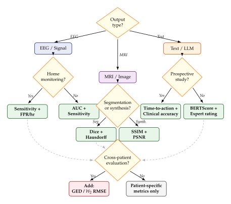
A Reproducibility Checklist for Epilepsy AI Papers
The following checklist consolidates the reproducibility requirements discussed in this section. Authors of epilepsy AI papers are encouraged to include a checklist table in supplementary materials; reviewers are encouraged to request it.
Dataset: Which dataset(s) were used? Which version or release? Were any subjects excluded, and why?
Splits: Are splits temporal or random? Are they at the epoch, session, or patient level? Are splits fixed and released alongside the paper?
Protocol: Patient-specific or cross-patient? If cross-patient, which subjects are in train/val/test?
Preprocessing: What filtering, normalisation, referencing, and artefact rejection were applied? Are preprocessing scripts released?
Architecture: Is the full architecture specified, including all layer sizes, activation functions, and normalisation strategies?
Hyperparameters: Are all hyperparameters reported, including learning rate schedule, batch size, dropout rates, augmentation parameters, and early stopping criteria?
Metrics: Are all metrics defined precisely, including how ties are broken, how multi-class problems are aggregated, and how the prediction horizon is defined for prediction tasks?
Statistical testing: Is performance reported with confidence intervals or standard errors across cross-validation folds or runs? Is a significance test performed?
Code: Is executable code released? Is it sufficient to reproduce the reported numbers from the released dataset?
Compute: What hardware was used? How long did training take? Are there estimates of energy consumption?
Insight.
The reproducibility checklist as a research accelerator. Counter-intuitively, investing in reproducibility accelerates research progress rather than slowing it. A paper that releases code, hyperparameters, and fixed splits becomes the foundation on which subsequent papers build. The BraTS challenge is the clearest example: because it enforced fixed splits and a hosted evaluation server, the segmentation community made more progress in five years (2015–2020) than it had in the preceding decade. The epilepsy AI community has not yet had its BraTS moment, but the infrastructure to create it already exists.
Exercises
Exercise 33 (Evaluating a Seizure Detector Under Different Protocols).
You are given 100 hours of EEG from a single patient containing 20 seizures, each of average duration 2 minutes. The remaining 98.3 hours are non-seizure. You train a seizure detector and obtain the following confusion matrix on a held-out test set consisting of the last 20 hours of data (4 seizures, 19.9 hours of non-seizure):
| Pred. Seizure | Pred. Non-seizure | |
| True Seizure | 3 | 1 |
| True Non-seizure | 4 |
Compute the sensitivity, specificity, and FPR/hr of this detector on the test set. (Treat each 30-second epoch as the unit of analysis; the test set contains 4 4 = 16 seizure epochs and non-seizure epochs.)
Suppose a colleague trained the same architecture on the same dataset but used a random 80/20 split at the epoch level. They report sensitivity = 98,% and specificity = 97,%. Explain in detail why their numbers are not comparable to yours and are likely inflated.
The dataset contains 20 seizures. An alternative evaluation protocol uses leave-one-seizure-out cross-validation: each seizure and its surrounding 2 hours form a test fold, and the model is retrained on the remaining 19 seizures. Write out the mathematical expression for the cross-validation estimate of sensitivity and FPR/hr under this protocol. What is a potential disadvantage compared to the temporal split used in part (a)?
For home monitoring applications, regulatory guidance suggests that a clinically acceptable detector should achieve sensitivity and FPR/hr . Does your detector in part (a) meet this standard? If not, which hyperparameters or architectural choices might you adjust, and what is the fundamental sensitivity/FPR trade-off you are navigating?
Exercise 34 (The Pseudo-Healthy Synthesis Evaluation Problem).
A diffusion model has been trained on 500 healthy subjects and is used to synthesise pseudo-healthy counterparts for 50 patients with FCD. For each patient, the residual map is computed as in equation . A neuroradiologist has provided binary FCD lesion masks for each patient.
Suppose you threshold the residual map at level to produce a binary lesion prediction . Define sensitivity and positive predictive value (PPV, also called precision) for this detector at the voxel level. Show that there is a fundamental trade-off: increasing increases PPV but decreases sensitivity. Sketch the resulting precision-recall curve for a qualitatively reasonable residual distribution.
The SSIM between the synthesised pseudo-healthy image and the true healthy scan of the same patient (obtained, say, from a healthy sibling) is proposed as an evaluation metric. Identify at least two confounds that make SSIM a problematic primary metric for this task, and propose a complementary metric that addresses each confound.
Let be the healthy distribution learnt by the diffusion model. You wish to test whether the residual for FCD patients is statistically larger than for healthy controls. Describe an appropriate permutation test for this hypothesis, specifying the test statistic, the permutation scheme, and the null distribution.
A critic argues that pseudo-healthy residual maps are fundamentally circular: they detect FCD only because the training set excluded FCD patients, so the model has never seen FCD tissue and cannot generate it. Therefore, any “detection” is simply the model failing to reconstruct pathological tissue, which could be triggered equally by imaging artefacts, motion, or scanner differences. Construct a rigorous experimental protocol to test whether the residual map provides information beyond scanner and motion artefact effects.
Exercise 35 (Optimal Transport Metrics for Connectivity Generalisation).
Let be a set of functional connectivity graphs from healthy subjects, and let be a set of graphs from patients with temporal lobe epilepsy (TLE). Each graph has nodes (AAL atlas regions) and edges weighted by pairwise Pearson correlation of resting-state fMRI BOLD signals.
Define the empirical distributions and . To compute as in equation , you need a ground metric on the space of graphs. Propose a ground metric that (i) is symmetric, (ii) satisfies the triangle inequality, and (iii) respects the semantic meaning of connectivity (i.e., graphs that differ only in weak edges should be closer than graphs that differ in hub-node connections). Justify your choice.
Computing exactly requires solving a linear programme of size . Describe the Sinkhorn algorithm as an approximate solver. How does the regularisation parameter in the entropy-regularised OT problem trade off computational speed against approximation quality? What value of would you recommend for this application, and why?
You propose using as a biomarker for disease severity in patient , where is the empirical distribution over multiple resting-state fMRI sessions of patient and is the fixed healthy reference distribution. Identify two potential confounders of this biomarker that arise from the fMRI acquisition process itself (not from the patient's pathology).
A cross-patient model is trained to predict deviation from a new patient's baseline EEG features. The model is evaluated using as in equation . Explain why alone is insufficient as an evaluation metric for this task. What additional metric would you report, and how would you compute it?
Open Problems and Future Directions
The preceding sections have established a comprehensive mathematical framework for generative AI in epilepsy research: GANs and diffusion models for seizure signal synthesis, VAEs for latent seizure manifolds, optimal transport for cross-patient normalisation, and transformers for long-range ictal dynamics. Across each of these domains, the frontier has advanced considerably in the past five years. Yet the gap between what is mathematically possible in controlled laboratory settings and what is clinically deployable at the bedside of a patient with drug-resistant epilepsy remains formidable.
This section identifies seven open problems that, in our assessment, represent the most important barriers to progress. We frame each problem as a precise mathematical question wherever possible, and we close with a conjecture about the structural nature of the solution space. The reader should treat these not as discouraging limitations but as an invitation: the next generation of breakthroughs in epilepsy AI will come from those who engage seriously with the hardest questions.
Key Idea.
The central challenge of generative epilepsy AI is not generative quality but clinical relevance. A diffusion model that synthesises EEG traces indistinguishable from real seizures is impressive but clinically useless unless it (a) runs fast enough for a wearable implant, (b) captures the idiosyncratic ictal dynamics of the individual patient, (c) transfers knowledge across patients without catastrophic forgetting, and (d) does so in a manner that satisfies the regulatory standards of the FDA and EMA. The open problems below address each of these requirements in turn.
Open Problem 1: Real-Time Generative Seizure Prediction for Implantable Devices
Approximately one-third of people with epilepsy do not achieve seizure freedom with medication (Brodie et al., 2012). For this population, implantable closed-loop neurostimulation devices offer hope: a device that detects the pre-ictal state and delivers a brief therapeutic stimulus before the seizure generalises. The NeuroPace RNS System and Medtronic Percept represent current-generation implementations. However, these devices use hand-crafted feature extractors and threshold classifiers. Generative models offer a fundamentally different paradigm: instead of classifying the current EEG into “pre-ictal” or “interictal”, a generative model would predict the likely future trajectory of the EEG signal and intervene when the predicted trajectory converges on a seizure attractor.
Definition 26 (Generative Seizure Predictor).
Let denote the multichannel iEEG signal observed up to time ( channels). A generative seizure predictor is a conditional model over future signal trajectories of horizon time steps, together with a decision rule (PRED Decision) where is the ictal state set estimated from historical seizures and is a sensitivity threshold. The predictor fires a stimulation pulse when .
The key obstacle is latency. Current diffusion-based sequence models require on the order of forward passes, where is the context window length and is the number of denoising steps. Even with (aggressive DDIM acceleration) and time points at 250,Hz (4 seconds of context), the computational budget on an implant with a 32-bit ARM cortex-M4 running at 64,MHz and a power budget of 50,W is exceeded by several orders of magnitude.
Open Problem 1.
Open Problem 1. Design a generative sequence model that:
runs inference in ,ms on a microcontroller with ,kB of SRAM;
maintains a false positive rate (to avoid therapy fatigue and tissue damage);
achieves sensitivity with horizon ,s (sufficient for pre-ictal stimulation).
No existing architecture simultaneously satisfies all three constraints. The key mathematical question is whether the expressive power of a model whose inference complexity is is sufficient to model the pre-ictal trajectory distribution, or whether sub-threshold seizure predictability requires fundamentally high-dimensional representations.
Promising directions.
Two lines of work appear most promising. First, neural architecture search (NAS) over quantised (4-bit or 8-bit integer) state-space models such as S4 or Mamba can discover architectures whose parameter footprints fit on-chip while retaining competitive classification performance. Second, amortised variational inference with a low-dimensional latent space (with ) can encode the pre-ictal trajectory in a compact representation that is cheap to update at each new sample. The trade-off between latent dimension and predictive accuracy is governed by the rate-distortion bound: (RATE Distortion) where is the rate-distortion function of the pre-ictal process and is the bit-rate of the latent code.
Open Problem 2: Personalized Brain Digital Twins via Generative Models
The epileptic brain is not a generic brain with an extra oscillation. Seizure onset zones differ between patients in location, extent, and connectivity. A generative model trained on population-level EEG will, at best, capture the average seizure phenotype. What is clinically needed is a personalized brain digital twin: a generative model calibrated to the specific neuroanatomy, connectivity, and seizure semiology of patient from a small number of observed seizures.
Definition 27 (Brain Digital Twin).
A brain digital twin for patient is a tuple , where:
is a patient-specific functional connectivity graph with nodes corresponding to electrode contacts, edges encoding white-matter tracts or coherence connections, and weight matrix ;
is a generative model of the patient's EEG signal conditioned on the graph structure: ;
is a low-dimensional phenotype vector encoding the patient's clinical covariates (age, epilepsy duration, antiseizure medication history).
The twin is valid if it satisfies: for a comprehensive set of test statistics (spectral, temporal, graph-theoretic).
The mathematical challenge is few-shot personalisation: each patient typically provides recorded seizures, an order of magnitude fewer than the thousands of examples needed to train a model from scratch. Meta-learning approaches such as MAML (Finn et al., 2017) frame personalisation as finding initial parameters such that a small number of gradient steps on patient 's data reaches a good personalised model: (MAML) where is the reconstruction loss on patient 's seizure data. Whether the seizure manifold has the geometry required for meta-learning (i.e., whether patient-specific optima lie close to a common initialisation in parameter space) is an empirically open question.
Open Problem 3: Cross-Patient Generalization Without Catastrophic Forgetting
A seizure detection model deployed in a clinical device must adapt continuously as new seizures are recorded. Each new seizure provides evidence about the patient's evolving ictal pattern (seizure semiology can change with disease progression and medication changes), yet the model must not forget the patterns learned from earlier data. This is the continual learning problem applied to EEG, but with additional cross-patient complexity: we want a model that accumulates knowledge across all patients without suffering from negative transfer.
Formally, let be a stream of patient datasets arriving sequentially. After learning on , the model should satisfy: (Continual) where is the oracle model trained exclusively on and is a tolerated forgetting budget. The tension is fundamental: gradient updates on will, in general, increase the loss on all previous .
Open Problem 2.
Open Problem 3. Develop a generative continual learning algorithm for cross-patient EEG that:
achieves AUC degradation on previously seen patients after learning 100 new patients;
does not require storing raw EEG from previous patients (for privacy);
scales to patients without increasing model capacity beyond a fixed budget of parameters.
Generative replay (Shin et al., 2017), wherein a generative model synthesises pseudo-rehearsal data from past tasks, is a natural candidate but has not been systematically evaluated for iEEG. The key question is whether the generative model (itself also subject to forgetting) can produce pseudo-rehearsal data of sufficient quality to prevent classifier forgetting.
The interaction between the generative model's forgetting and the classifier's forgetting creates a coupled dynamical system that has received little theoretical attention. An analysis leveraging the Fisher information matrix of the generative model (elastic weight consolidation applied to generative models, EWC-Gen) may yield tight forgetting bounds.
Open Problem 4: Ethical Synthetic EEG - Deepfake Risks and Regulatory Traceability
Synthetic EEG generation, developed throughout this chapter as a tool for data augmentation and privacy preservation, carries a dual-use risk that has received insufficient attention. A high-fidelity EEG generator trained on seizure data from a specific patient could, in principle, produce traces that: (a) mislead a physician into diagnosing epilepsy in a healthy individual; (b) fabricate forensic evidence of a neurological event; or (c) fool a clinical AI system into prescribing antiseizure medication or authorising a disability claim.
Caution.
Synthetic EEG can be weaponized. Establish provenance protocols before deployment. The FID scores and power spectral densities reported in the synthetic EEG literature establish that current GAN and diffusion models produce traces that are statistically indistinguishable from real recordings to automated classifiers. This is presented as evidence of generation quality; it is simultaneously evidence that these generators can produce convincing fabrications. Unlike synthetic text or synthetic images, synthetic EEG is used in high-stakes medical and legal contexts where fabrications can cause direct patient harm. Any laboratory that publishes a high-fidelity EEG generator bears a responsibility to: (1) embed cryptographic provenance watermarks in all generated traces, (2) publish an authenticated detector alongside the generator, and (3) not release training code that would allow fine-tuning on a specific patient's data without institutional ethics approval.
The mathematical foundation for provenance is steganographic watermarking of generated signals. A differentiable watermark embeds a unique identifier into the generated signal such that the watermark is (i) imperceptible (the spectral distortion ), (ii) robust to clinical signal processing (bandpass filtering, re-referencing, artifact rejection), and (iii) recoverable by an authorised detector with bit accuracy . The trade-off between imperceptibility and robustness to processing is characterised by a watermarking rate-distortion function analogous to Equation .
Open Problem 3.
Open Problem 4. Design a provenance watermarking scheme for synthetic EEG that:
embeds at least bits of provenance information (generator ID, date, patient cohort, institutional IRB number);
is spectrally imperceptible (V RMS across all frequencies ,Hz);
survives standard EEG preprocessing (notch filter, bandpass, ICA artifact rejection) with recovery accuracy ;
is computationally cheap to embed at generation time (,ms additional inference cost).
Open Problem 5: Unified Multimodal Foundation Model for Epilepsy (EEG + MRI + Clinical Text)
Current epilepsy AI systems operate in modality-specific silos. A scalp EEG classifier is trained on EEG. An MRI-based lesion detector is trained on volumetric scans. A clinical NLP system extracts seizure semiology from clinic notes. Each system reaches independent conclusions that a neurologist must integrate mentally. The vision of a unified multimodal foundation model for epilepsy is a single model that jointly encodes all available modalities and produces a unified clinical assessment.
The generative perspective adds an important dimension. Rather than a discriminative model, we want a generative model over the joint observation space conditional on the clinical label (e.g., epilepsy syndrome type, seizure onset zone, medication response). Such a model supports not only classification but cross-modal synthesis (generate the expected EEG given an MRI lesion map), imputation (infer missing MRI from EEG and clinic notes), and counterfactual reasoning (what would the EEG look like if the patient underwent a successful resection?).
Definition 28 (Epilepsy Multimodal VAE).
Let be a shared latent representation. The epilepsy multimodal VAE factorises as: (Mmvae Encoder) where is the EEG spectrogram, is the structural MRI, and is the clinical narrative text (represented as a BERT embedding). The modality-specific decoders (1D temporal), (3D volumetric), and (discrete token sequence) have heterogeneous architectures but share the latent space .
Open Problem 4.
Open Problem 5. Build and validate a unified multimodal foundation model for epilepsy pre-surgical evaluation that:
improves seizure onset zone localisation accuracy (measured against post-operative outcome) by over the best unimodal baseline;
provides calibrated uncertainty over the predicted onset zone (reliability diagram error );
handles arbitrary subsets of available modalities via product-of-experts or mixture-of-experts inference;
is trained on data from independent epilepsy centres with federated learning to avoid privacy violations.
The critical architectural challenge is aligning modalities with fundamentally different temporal scales (EEG at 256,Hz versus MRI as a static volume) within a single latent space.
Open Problem 6: Causal Generative Models for Understanding Seizure Mechanisms
Generative models of seizure activity are currently associative: they learn or but cannot answer interventional or counterfactual questions (Pearl's second and third rungs of the causal hierarchy). A clinician facing a pre-surgical evaluation does not want to know what seizures look like in general; she wants to know: “If I resect electrode contacts 12–15 in this patient, will seizures stop?” This is a counterfactual query that no purely associative generative model can answer.
A causal generative model of seizure dynamics would encode the structural equations governing ictal propagation: (SCM) where is the EEG signal at electrode , denotes the causal parents of in the ictal propagation graph , and is an independent exogenous noise variable. Intervening on node (ablating it) corresponds to replacing with the constant and simulating the resulting altered dynamics.
The challenge is that the causal graph of seizure propagation is latent: it must be inferred from observed EEG. Causal discovery algorithms such as PC or FCI are designed for static variables, not for time series with non-linear, non-stationary dynamics.
Open Problem 5.
Open Problem 6. Develop a causal generative model for seizure propagation that:
infers the ictal propagation graph from intracranial EEG using a differentiable causal discovery objective (e.g., NOTEARS or DAG-GNN adapted to time series);
supports counterfactual simulation of post-resection EEG with calibrated uncertainty;
validates predicted post-resection EEG against observed post-operative interictal recordings in a cohort of patients with known surgical outcomes.
Success on this problem would represent a qualitative advance: from generative models as data augmentation tools to generative models as mechanistic simulators of epileptic networks.
Open Problem 7: Optimal Transport-Guided Neuromodulation (Closed-Loop DBS)
Deep brain stimulation (DBS) and responsive neurostimulation (RNS) deliver electrical pulses to suppress aberrant oscillations associated with seizures. The current generation of closed-loop devices use threshold-based triggers: stimulation fires when a detector exceeds a predetermined amplitude or power threshold. This reactive paradigm intervenes after the ictal process has begun.
A more principled approach, as yet unrealised, would use the generative model to compute the optimal transport map from the current ictal EEG distribution to the desired interictal EEG distribution and drive the stimulation waveform along the geodesic connecting the two distributions in the Wasserstein space .
Definition 29 (OT-Guided Stimulation Policy).
Let denote the distribution of the multichannel EEG at time (estimated via a streaming particle filter), and let be the target interictal distribution. The OT-guided stimulation policy at time is: (OT STIM Policy) and the stimulation waveform is the infinitesimal displacement that moves along the Wasserstein geodesic toward : (OT Waveform) where is the Brenier map (Villani, 2008).
The main computational obstacle is that the Brenier map must be computed and updated in real time (at 1,kHz stimulation frequency) from streaming EEG data. Neural OT solvers (Makkuva et al., 2020; Rout et al., 2022) provide amortised approximations but have not been validated in closed-loop neuromodulation settings.
Open Problem 6.
Open Problem 7. Demonstrate in an animal model of temporal lobe epilepsy that OT-guided stimulation:
reduces seizure duration by compared to threshold-based reactive stimulation;
requires stimulation energy that of conventional DBS (energy efficiency is critical for battery-powered implants);
can be computed online with ,ms latency using a neural OT solver running on an FPGA.
Conjecture: No Single Generative Architecture Will Dominate All Epilepsy Tasks
The history of machine learning is punctuated by epochs of apparent universal dominance: convolutional networks in the 2010s, then transformers from 2017, then diffusion models from 2021. Each transition was followed by a period of evangelism during which practitioners applied the dominant architecture uniformly across all domains. We conjecture that this pattern will not hold for epilepsy AI.
Conjecture 1 (No Single Architecture Dominates Epilepsy Tasks).
Let GAN, VAE, diffusion, transformer, flow, OT denote the set of generative architectures, and let seizure synthesis, data augmentation, seizure prediction, brain twin, cross-modal synthesis, closed-loop control denote the set of epilepsy tasks. For any architecture , there exists a task such that is not Pareto-optimal on with respect to the joint objective of accuracy, latency, and sample efficiency. In particular:
GANs dominate for high-throughput data augmentation where per-sample generation speed is paramount;
diffusion models dominate for high-fidelity seizure synthesis where perceptual quality and diversity matter;
VAEs dominate for latent space interpolation and brain twin personalisation where a smooth, structured latent geometry is required;
optimal transport dominates for closed-loop neuromodulation where the target distribution is known and direct geodesic control is required;
transformers dominate for long-range ictal dependency modelling where context windows exceeding 30,s are needed.
The practical implication is that the field should invest in compositional architectures that combine the strengths of multiple paradigms rather than competing to crown a single successor. The mathematical challenge is to design composition interfaces: latent spaces, message-passing protocols, and objective functions that allow, for example, a VAE brain twin to feed a conditioning signal to an OT-guided stimulator via a diffusion posterior sampler.
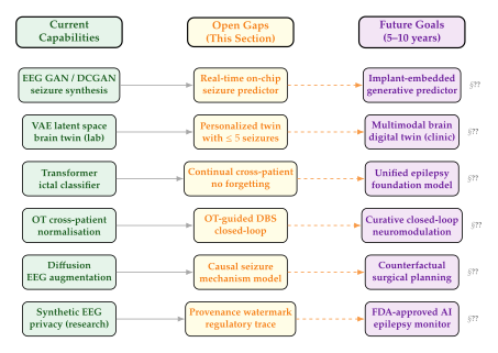
Clinical Translation and Ethics
The seven open problems of the preceding section are scientific. But the path from a published algorithm to a tool that changes the life of a patient with drug-resistant epilepsy also traverses a thicket of regulatory, ethical, legal, and societal challenges. This section addresses these challenges directly. We organise them around four themes: the FDA regulatory pathway, privacy and synthetic data, demographic bias in EEG datasets, and explainability of generative latent spaces.
Key Idea.
Clinical translation is not a post-hoc step; it must be designed in from the beginning. A generative EEG model designed without regulatory constraints will need to be redesigned when those constraints are eventually encountered. A synthetic EEG dataset built without privacy analysis will be vulnerable to membership inference attacks. A seizure detection system trained without demographic stratification will perform worse on women and children, the very populations with the highest burden of drug-resistant epilepsy. The best time to address clinical translation requirements is at the design stage, not during FDA review.
FDA Regulatory Pathway for AI in Neurology
The United States Food and Drug Administration regulates AI-based neurological devices under 21 CFR Part 882 (neurological devices). Three regulatory pathways are relevant:
- 510(k) Premarket Notification.
Available when the device is substantially equivalent to a legally marketed predicate device. For an AI seizure detector, the predicate might be a cleared ambulatory EEG monitor (e.g., Natus Quantum). The 510(k) pathway requires demonstrating equivalent sensitivity/specificity but does not require randomised controlled trial (RCT) evidence. Turnaround is typically 3–6 months.
- De Novo Classification.
For AI devices with no substantially equivalent predicate, the De Novo pathway creates a new regulatory classification with special controls. The FDA's 2021 Artificial Intelligence/ Machine Learning (AI/ML) Action Plan and the subsequent Predetermined Change Control Plan (PCCP) framework are particularly relevant for adaptive AI systems that update their parameters based on post-deployment data.
- Premarket Approval (PMA).
Required for high-risk Class III devices, including implantable closed-loop neurostimulators. PMA requires valid scientific evidence including one or more RCTs. For an OT-guided DBS system (Open Problem 7), PMA is the required pathway, typically requiring 5–10 years of clinical development.
Software as a Medical Device.
The FDA's Software as a Medical Device (SaMD) framework, developed in collaboration with the International Medical Device Regulators Forum (IMDRF), classifies AI software by the severity of the condition it addresses and the criticality of the decision it supports. A generative EEG system that informs a physician's diagnosis (rather than making autonomous decisions) falls under lower-risk SaMD classification, significantly easing the regulatory burden. This design choice - keeping the clinician in the loop - has regulatory advantages beyond the ethical ones.
The critical issue for generative models specifically is locked versus adaptive algorithms. The FDA's 2021 guidance distinguishes:
Locked algorithms: the model does not change after deployment. Standard regulatory controls apply.
Adaptive algorithms: the model updates based on real-world performance data. A PCCP must be submitted specifying the anticipated modifications, the performance monitoring strategy, and the retraining boundaries.
For a generative brain twin (Open Problem 2) that personalises to a patient's new seizures over time, the adaptive pathway is essential. The PCCP must specify: what triggers a model update (e.g., new seizures recorded), what data is used for retraining, and what performance validation is performed before the updated model is activated.
Privacy: HIPAA, GDPR, and Synthetic Data as a Privacy Solution
Intracranial EEG is Protected Health Information (PHI) under HIPAA and Special Category Personal Data under GDPR Article 9 (data revealing health information). Sharing iEEG datasets across institutions for collaborative model training requires either (a) a Data Use Agreement (DUA) covering de-identification, (b) federated learning that keeps raw data on-site, or (c) synthetic data generation as a privacy-preserving surrogate.
Synthetic EEG offers an attractive third option: train a generative model on real iEEG under institutional approval, then release the synthetic dataset publicly without a DUA. However, this approach is only as strong as the privacy guarantee of the generative model.
Definition 30 (Differential Privacy for Generative EEG).
A generative model is -differentially private with respect to a training dataset if, for all adjacent datasets (differing in one patient's data) and all sets of generative model outputs: (DP) The DP-SGD algorithm (Abadi et al., 2016) achieves this by clipping per-sample gradients to norm and adding calibrated Gaussian noise: (DP SGD) where is the mini-batch, is the clipping norm, and is calibrated to achieve the desired guarantee via the moments accountant.
In practice, applying DP-SGD to EEG generative models introduces a quality-privacy trade-off. At (strong privacy), generative model FID typically degrades by 30–50% compared to the non-private baseline. At (weak privacy, often considered insufficient for medical data), the FID gap reduces to . Determining the appropriate budget for synthetic iEEG is an unresolved policy question: existing HIPAA de-identification standards do not map directly onto the framework.
A complementary approach to DP-SGD is membership inference auditing: after training, an adversary attempts to determine whether a specific patient's data was in the training set. The audit provides an empirical privacy bound independent of the theoretical DP analysis. Shokri et al.'s (2017) shadow training attack and the LiRA attack (Carlini et al., 2022) are the standard auditing tools. A synthetic EEG dataset should only be released publicly if the best known membership inference attack achieves AUC (close to random chance) on the training cohort.
Bias: Demographic Underrepresentation in EEG Datasets
The canonical scalp-EEG dataset used to benchmark seizure detection algorithms is the CHB-MIT Scalp EEG Database, containing recordings from 23 paediatric patients at Boston Children's Hospital (Shoeb, 2009). More recent benchmarks include the Temple University EEG Corpus (TUEG) with over 25,000 sessions. Despite their size, these datasets share a structural bias: they predominantly represent patients from high-income, English-speaking countries who were able to access tertiary epilepsy centres.
The clinical consequences of this bias are measurable. Seizure detection models trained on CHB-MIT achieve substantially lower sensitivity in:
Adult patients, because paediatric seizure morphology (higher amplitude, more stereotyped) differs from adult seizure morphology;
Female patients, due to hormonal modulation of seizure threshold (catamenial epilepsy) and differences in ictal semiology;
Non-focal epilepsies, because hospital-based datasets over-represent lesional focal epilepsy (surgically amenable, hence disproportionately evaluated at centres with iEEG capability).
Generative debiasing.
Generative models offer a principled approach to dataset debiasing: synthesise data for underrepresented subgroups until the joint distribution of EEG morphology and demographic covariates is approximately balanced. Formally, let where is a sensitive attribute (age group, sex, epilepsy syndrome). The generative debiasing objective is: (Debias) i.e., the conditional EEG distribution given each attribute should match the real distribution, but the marginal over attributes should be uniform. Conditional GANs and conditional diffusion models with attribute conditioning (class-free guidance) are natural implementations.
The validation challenge is circular: if no real data exists for the underrepresented subgroup, how can we verify that the synthetic data is realistic? This requires engagement with epilepsy centres in under-represented regions (Africa, South Asia) and with community-based EEG screening programmes, not purely algorithmic solutions.
Explainability: Interpreting Diffusion Attention Maps and Latent Spaces
Regulators and clinicians require that an AI system's decisions be explainable. The FDA's 2021 AI/ML Action Plan specifically cites explainability as a key element of transparency. For discriminative classifiers, attribution methods such as Grad-CAM, SHAP, and integrated gradients are well established. For generative models, explainability is less mature but arguably more important: if a diffusion model generates a “typical pre-ictal EEG”, the clinician needs to understand which features of that EEG are being highlighted.
Diffusion attention analysis.
In text-conditioned diffusion models, the cross-attention maps at denoising layer (where is the number of signal patches and is the number of text tokens) indicate which parts of the EEG signal attend to which clinical descriptors. Aggregated attention maps provide a free explanation: “this generated seizure segment is most influenced by the token ictal tachycardia in channels 4, 7, and 12.” The mathematical operation is: (Attention Attribution) where the average is over denoising steps . High indicates that signal patch is a primary driver of the generation at layer .
Latent space disentanglement.
For VAE-based brain twins, clinical interpretability requires that individual latent dimensions correspond to clinically meaningful factors: seizure duration, spread pattern, dominant frequency, amplitude. Total Correlation Variational Autoencoder (-TCVAE; Chen et al., 2018) encourages disentanglement by penalising the total correlation: (Tcvae) A latent dimension is interpretable if there exists a clinically defined feature (e.g., dominant frequency) such that the Spearman rank correlation across a validation cohort. Ensuring interpretability without sacrificing generative quality (the classical disentanglement-quality trade-off) remains an active research area.
Exercises and Research Challenges
The exercises below consolidate the mathematical and conceptual foundations developed throughout this chapter. They progress from focused calculations (Exercises 1–5) through synthesis-level problems (Exercises 6–10) to open-ended research challenges (Challenges 1–3). We recommend that readers attempt every part independently before consulting the references.
Key Idea.
Difficulty Progression Exercises 1–5 focus on core mathematical tools: GAN training dynamics, diffusion augmentation, Wasserstein distances, transformer channel selection, and the VAE-EEG ELBO. Exercises 6–10 address applied synthesis: cross-modal evaluation, clinical triage algorithm design, optimal transport on persistence diagrams, privacy analysis, and benchmark design. Research Challenges 1–3 require building complete systems.
Exercise 36 (GAN Training Dynamics for EEG).
Consider a vanilla GAN trained on single-channel scalp EEG segments of length samples (1 second at 256,Hz). The generator maps a Gaussian latent vector to an EEG segment. The discriminator outputs a probability that its input is real.
Minimax objective. Write the minimax objective for the GAN: (GAN Objective) Show that at the Nash equilibrium, the generator distribution satisfies and the optimal discriminator is everywhere. State clearly which assumption about is required for the optimality proof to go through.
Mode collapse in EEG. An EEG dataset contains seizure segments from three distinct seizure types: temporal lobe (TL), frontal lobe (FL), and generalised tonic-clonic (GTC), with frequencies 25%, 35%, and 40% respectively. After 10,000 GAN training steps, the generator produces exclusively GTC-type segments. enumerate[label=()]
Define the mode coverage metric as the entropy of the distribution over seizure types in the generated samples: . Compute for the collapsed generator and for a perfectly diverse generator.
Propose a modification to the training objective, using a diversity regulariser , that penalises mode collapse. One candidate is the minibatch discrimination term: (Minibatch) Explain why minimising discourages collapse.
Implement (in pseudocode) a training loop that alternates discriminator update and generator update with the augmented loss for . enumerate
Spectral fidelity. Let and denote the average power spectral densities (PSDs) of generated and real EEG segments respectively, estimated via Welch's method. Define the spectral fidelity score as: (Spectral Fidelity) with ,Hz. Show that with iff almost everywhere. Compute for a generator that outputs pure white noise () when the real EEG has a spectrum with and .
Convergence analysis. The WGAN-GP training objective (Gulrajani et al., 2017) is: (WGAN GP) where with . Explain why the gradient penalty enforces the 1-Lipschitz constraint on . Under what conditions on the learning rate and the number of discriminator steps per generator step does WGAN-GP training converge?
Exercise 37 (Diffusion Augmentation Pipeline for Seizure Detection).
A seizure detection classifier is trained on a dataset with ictal segments and interictal segments. You propose to balance the dataset using a diffusion model trained on the ictal segments.
Forward process. The forward diffusion process adds Gaussian noise according to: (Forward) For a linear noise schedule with , , : compute and . At what step does the signal-to-noise ratio fall below 0.01 (i.e., the signal is essentially noise)?
ELBO decomposition. The variational lower bound for the diffusion model is: (Diffusion ELBO) Show that each KL term can be evaluated in closed form when both distributions are Gaussian, and express the optimal reverse mean in terms of a noise-prediction network .
Augmentation benefit analysis. Let denote the seizure detector AUC when trained with synthetic ictal samples added. Empirically, for some . Determine the number of synthetic samples needed such that the marginal AUC gain from the -th synthetic sample falls below 0.001, as a function of and .
Overfitting risk. When training a diffusion model on only ictal segments, the model may memorise training examples rather than generalise. Define a memorisation score based on the nearest-neighbour distance in spectrogram space: (Memorisation) where are generated samples and is a copying threshold. Discuss how , the model capacity (number of parameters), and the noise schedule choice (linear vs cosine) affect .
Exercise 38 (Wasserstein Distance Between EEG Distributions).
Let and be empirical EEG distributions in (with representing frequency-band feature vectors). You wish to compute between interictal and pre-ictal EEG populations.
Primal formulation. Write the primal formulation of the 2-Wasserstein distance: (W2 Primal) where . Explain why direct solution via linear programming is infeasible for EEG segments.
Sinkhorn regularisation. The entropy-regularised problem is: (Sinkhorn) State the Sinkhorn algorithm for computing the optimal , including the kernel matrix and the alternating scaling updates for vectors and . Show that as .
Computational complexity. Derive the per-iteration computational cost of Sinkhorn as matrix-vector products. For and , estimate the wall-clock time needed for 100 Sinkhorn iterations on a single GPU with 10 TFLOPS of FP32 throughput. Compare with the exact LP solver.
Clinical interpretation. Suppose and (in standardised feature units). What does this ratio tell you about the structure of the pre-ictal transition? Design a sequential test based on monitoring over a sliding window and derive the threshold that controls the false positive rate at 1 per hour given a reference null distribution.
Exercise 39 (Transformer Channel Selection for iEEG).
A transformer-based seizure classifier operates on a multichannel iEEG tensor with electrode contacts and time points. Each channel is embedded as a sequence of non-overlapping patches of length .
Attention complexity. The standard self-attention mechanism computes: (Attention) where and tokens. Compute the total FLOPs required for one attention layer (for a single head) as a function of and . For , how much memory (in GB) is required to store the attention matrix in FP32?
Sparse attention. To reduce memory, you restrict attention to a neighbourhood of radius channels around each electrode (in terms of cortical distance). Show that this reduces the attention complexity from to . For (10 neighbouring contacts), compute the speedup and memory savings.
Channel importance attribution. After training, you extract the attention weights and compute the channel relevance score: (Channel Relevance) i.e., the total attention weight flowing to patches of channel from all other patches. Prove that (the sum is the total attention mass).
Electrode reduction. You wish to select the channels with the highest scores and retrain the classifier. Using the Gumbel-softmax trick for differentiable channel selection, write the reparameterised selection distribution and the resulting training objective. Discuss the trade-off between and classification AUC, and how you would determine the minimal needed for clinical deployment (fewer electrodes mean less invasive surgery).
Exercise 40 (ELBO Derivation for the VAE-EEG Model).
Let be a multichannel EEG seizure segment and a continuous latent code. The VAE-EEG model specifies: (VAE Prior)
ELBO derivation. Starting from the marginal log-likelihood , apply Jensen's inequality to obtain the ELBO: (ELBO) Identify the reconstruction term and the regularisation term, and explain their roles in the EEG context.
Closed-form KL. Show that for the Gaussian encoder and prior , the KL term has the closed form: (KL Closed)
Reparameterisation trick. Explain why the gradient cannot be computed directly by Monte Carlo. State the reparameterisation: with , and show that the resulting estimator is unbiased and has lower variance than the REINFORCE estimator.
-VAE for EEG. The -VAE objective is . For , describe qualitatively how the learned latent space will differ from the case. In the EEG context, which value of would you prefer for (i) generating high-fidelity synthetic seizures, and (ii) learning an interpretable representation of seizure type? Justify your answers.
Exercise 41 (Evaluation of EEG-to-fMRI Cross-Modal Synthesis).
A conditional generative model is trained to synthesise BOLD fMRI activation maps from simultaneous EEG recordings during seizures.
FID for volumetric data. The Frechet Inception Distance (FID) is defined as: (FID) where and are the mean and covariance of real and generated activation maps in the feature space of a 3D convolutional encoder. Discuss the challenges of adapting FID from 2D images to 3D fMRI volumes, including the choice of 3D encoder, the computation of for large matrices, and the sample size required for a stable FID estimate.
Structural similarity. The Structural Similarity Index (SSIM) between real and generated is: (SSIM) where are stability constants. Explain why SSIM alone is insufficient to evaluate cross-modal synthesis (i.e., a blurry mean fMRI map can achieve high SSIM but low clinical utility). Propose a complementary metric based on the Pearson correlation of activation z-scores in clinically defined ROIs (e.g., hippocampus, insula).
Clinical concordance. Neurologists evaluate fMRI seizure maps by whether the activation peak lies within 10,mm of the surgically confirmed seizure onset zone. Design a concordance metric for threshold ,mm. Estimate the sample size needed to detect a difference between two generative models at significance and power using a one-sided binomial test.
Bias-variance trade-off in synthesis. Show that the expected mean squared error of the synthesised fMRI map decomposes as: (BIAS Variance) Relate the bias and variance terms to properties of the generative model: a model with high decoder capacity and low KL weight will have low bias but high variance; a model with strong KL regularisation will have high bias but low variance. Determine the optimal in the -VAE framework that minimises total MSE.
Exercise 42 (Designing a Clinical Triage Algorithm Using Synthetic EEG).
You are asked to design a clinical triage algorithm that uses a generative EEG model to stratify patients referred for epilepsy evaluation into three risk tiers: urgent (refer for immediate iEEG implantation), routine (standard outpatient EEG monitoring), and low-priority (unlikely epilepsy, reassurance appropriate).
Likelihood ratio triage. Let and be the likelihoods of an EEG segment under models trained on ictal and interictal data respectively. Define the triage rule using the log-likelihood ratio: (LLR) Specify thresholds that assign patients to the three tiers. Express the expected cost of each tier assignment in terms of the false positive rate, false negative rate, and the clinical costs of unnecessary iEEG implantation and missed diagnosis.
Calibration. The triage algorithm outputs a risk score . Define the calibration error as the expected difference between predicted risk and actual seizure prevalence: (Calibration) where is the -th confidence bin. Propose a temperature scaling procedure to calibrate and derive the optimal temperature .
Cost-sensitive threshold selection. Let and denote the costs of a false positive (unnecessary procedure) and false negative (missed seizure). Show that the optimal decision threshold minimises the expected cost: (COST Threshold) where is the prevalence of epilepsy in the triage population. For and , determine from a given ROC curve and compute the operating sensitivity and specificity.
Prospective validation design. Describe the key elements of a prospective multi-centre study to validate the triage algorithm: primary endpoint, sample size calculation, control arm, and stopping rules. What pre-registration conditions would the FDA require before accepting this study as evidence for De Novo clearance?
Exercise 43 (Optimal Transport on EEG Persistence Diagrams).
Topological data analysis (TDA) characterises the shape of seizure activity through persistence diagrams. Let be the persistence diagram of an EEG segment in dimension (computed via the Vietoris-Rips filtration on the electrode contact point cloud).
Bottleneck and Wasserstein distances. The -Wasserstein distance between persistence diagrams and is: (Persistence Wasserstein) where ranges over partial matchings (unmatched points are matched to the diagonal ). Describe the Hopcroft-Karp algorithm for computing the bottleneck distance () in time. When does the bottleneck distance fail to detect meaningful differences between ictal and interictal persistence diagrams?
Stability theorem. State the stability theorem for persistence diagrams: for functions on a topological space . Interpret this in the EEG setting: what does it imply about the sensitivity of the persistence diagram to small perturbations of the EEG signal?
Sliced Wasserstein approximation. For large persistence diagrams ( points), direct computation of is expensive. The Sliced Wasserstein distance projects each diagram onto random lines and averages 1D Wasserstein distances: (Sliced Wasserstein) where is projection onto direction . Show that can be approximated in time with random projections, and determine such that the approximation error is with probability .
Discriminative power. You compute persistence diagrams for ictal and interictal EEG segments and compute the pairwise matrix. Describe a permutation test to determine whether the between-class distances are significantly larger than within-class distances. State the null hypothesis, the test statistic, and the approximation needed when is computationally infeasible.
Exercise 44 (Privacy Analysis of Synthetic EEG via Membership Inference).
A GAN trained on patients' ictal EEG segments is released as open-source. An adversary attempts to determine, for a target patient's EEG segment , whether was in the training set.
Shadow training attack. Describe Shokri et al.'s (2017) shadow training attack: train shadow GAN models on synthetic training sets that either include or exclude , then train a binary classifier on the discriminator scores to infer membership. What is the computational cost of the attack as a function of and the GAN training time ?
Likelihood ratio test. The LiRA attack (Carlini et al., 2022) uses the ratio: (LIRA) Show that for a Gaussian likelihood model, reduces to a function of the log-likelihood of under compared to its expected log-likelihood under the null (non-member) distribution. Derive the resulting threshold rule.
DP guarantee. If the GAN is trained with DP-SGD at , what is the theoretical upper bound on the membership inference advantage of any adversary? Specifically, show that: (DP MI Bound) where is the minimum membership prior. For and , compute the numerical bound.
Practical audit. Design a practical privacy audit for the open-source GAN: specify the auditing dataset (how many members and non-members), the attack model architecture, the evaluation metric (AUC of the membership classifier), and the acceptance threshold for public release (AUC ). Discuss what additional safeguards (access controls, query rate limits) should accompany release of the model weights even if the audit passes.
Exercise 45 (Designing a Reproducible Benchmark for Generative Epilepsy AI).
The field of generative EEG modelling suffers from a lack of standardised benchmarks: papers use different datasets, different train/test splits, and different evaluation metrics, making progress difficult to track.
Benchmark design principles. Enumerate five principles for a reproducible benchmark, drawing on the ImageNet, BraTS, and PhysioNet benchmark design literature. For each principle, give a concrete instantiation for the synthetic EEG setting. Specifically address: (i) train/validation/test split strategy, (ii) stratification by seizure type and patient demographics, (iii) held-out test sets for which labels are not publicly released, (iv) multiple evaluation metrics covering fidelity, diversity, and clinical utility, and (v) a standard preprocessing pipeline.
Evaluation metric suite. Propose an evaluation metric suite for synthetic seizure EEG, including: enumerate[label=()]
at least one distribution-level metric (e.g., FID, MMD, or Wasserstein);
at least one clinical utility metric (e.g., seizure detection AUC on a downstream classifier trained exclusively on synthetic data);
at least one diversity metric (e.g., mode coverage, intra-class variation);
at least one privacy metric (e.g., membership inference AUC);
the spectral fidelity score from Exercise 36(c). enumerate Discuss how to aggregate into a single overall score, and the problems with any such aggregation.
Statistical comparison. Given benchmark results for two models and over five seeds each, describe a bootstrap hypothesis test to determine whether significantly outperforms on the clinical utility metric. State the null hypothesis, the test statistic, and the correction needed for multiple comparisons across the full metric suite .
Living benchmark. Propose a governance structure for a living benchmark that updates its test set annually to prevent overfitting of the field to a fixed test partition. How should historically submitted model scores be adjusted when the test set changes? What is the minimum number of new test examples needed to maintain statistical stability?
Research Challenges
The following challenges represent frontier research directions requiring original contributions. Each challenge is designed to be the basis of a graduate research project or dissertation chapter. We provide context, desiderata, and evaluation criteria but deliberately leave the solution approach open.
Challenge 2 (Building a Mini Seizure Prediction System for a Wearable Device).
Context. The gap between laboratory seizure prediction algorithms and implantable or wearable devices is dominated not by accuracy but by computational constraints. Current state-of-the-art seizure prediction models (e.g., transformer-based iEEG classifiers) require gigabytes of GPU memory at inference time and watt-scale power, while a behind-the-ear wearable scalp EEG device operates at milliwatt budgets with kilobyte-scale SRAM.
The Challenge. Design, train, and evaluate an end-to-end seizure prediction pipeline that satisfies:
Accuracy: sensitivity with false alarm rate /hour on the CHB-MIT database, evaluated under the five-fold patient-independent protocol.
Latency: inference time ,ms per 30-second EEG window on an ARM Cortex-M55 (or equivalent microcontroller emulation) at 64,MHz.
Memory: total model footprint (weights + activations) ,kB.
Power: estimated power consumption (using manufacturer-provided energy-per-MAC figures) ,mW in continuous monitoring mode.
Generativity: the predictor must output not just a binary alarm but a predicted EEG trajectory for ,s that allows the treating physician to inspect the expected pre-ictal evolution.
Technical Directions.
Architecture search. Use neural architecture search (NAS) over the space of quantised state-space models (S4, Mamba, xLSTM) with 4-bit integer quantisation. Constrain the search space to models with at most parameters and 8 recurrent state dimensions.
Generative compression. Train a VAE on the full-precision prediction model's hidden states, then distil the VAE decoder into a 3-layer MLP. The MLP decoder serves as the on-device trajectory predictor; the encoder is run off-device (in a paired smartphone) to update the latent prior.
Knowledge distillation. Train a large teacher model (e.g., a 12-layer temporal transformer with full-precision weights) on the combined CHB-MIT + Temple University EEG Corpus dataset. Distil the teacher into a quantised student of the target footprint using the distillation loss from Equation adapted to EEG trajectories.
Evaluation.
Benchmark accuracy on CHB-MIT using the standard leave-one-patient-out protocol.
Profile model footprint and latency on an ARM Cortex-M55 development board (or via CMSIS-NN emulation).
Evaluate the quality of predicted trajectories via the spectral fidelity score (Exercise 36(c)) and the Wasserstein distance to real pre-ictal segments.
Conduct a structured clinical review of ten predicted trajectories by a board-certified epileptologist.
Challenge 3 (Designing a Cross-Modal EEG-to-fMRI Generator for Seizure Onset Localisation).
Context. Simultaneous EEG-fMRI is the gold standard for non-invasive seizure onset localisation: the EEG provides temporal precision (millisecond resolution) while fMRI provides spatial resolution (millimetre-scale BOLD maps). However, simultaneous EEG-fMRI requires specialised MRI-compatible EEG equipment, scanner time costs of $500–2000/hour, and produces severely corrupted EEG (gradient artefacts, ballistocardiographic artefacts). A generative model that synthesises plausible fMRI activation maps from standard scalp or intracranial EEG alone would have immediate clinical value.
The Challenge. Develop a conditional generative model that:
achieves concordance (synthesised fMRI peak within 10,mm of the surgically confirmed seizure onset zone in of cases);
provides a voxel-level uncertainty map such that the actual BOLD map falls within the synthesised credible region in of voxels;
runs inference in ,s per patient on a single A100 GPU;
requires no simultaneous EEG-fMRI at inference time (only EEG is available).
Technical Directions.
Multimodal diffusion. Train a latent diffusion model conditioned on EEG embeddings. The conditioning is provided by a pre-trained EEG transformer encoder (frozen after EEG-only pre-training) via cross-attention in each diffusion U-Net block.
Haemodynamic response alignment. The EEG-fMRI relationship is mediated by the haemodynamic response function (HRF): (HRF) where is the canonical HRF and is the neural activity. Incorporate this temporal prior into the diffusion model's conditioning as a physics-informed constraint, either via a differentiable HRF convolution layer or as an auxiliary loss.
Unpaired training. Since paired EEG-fMRI datasets are scarce ( patients worldwide with simultaneous EEG-fMRI during seizures), explore cycle-consistency training using unpaired EEG-only () and fMRI-only () datasets. Define the cycle-consistency loss: (Cycle) and discuss the identifiability conditions under which cycle-consistency training recovers the true cross-modal relationship.
Evaluation.
Primary metric: evaluated on a held-out cohort of patients with both simultaneous EEG-fMRI and surgical outcome data.
Secondary metrics: voxel-level SSIM, FID (3D encoder), and concordance correlation coefficient between synthesised and real BOLD maps in seizure-related ROIs.
Clinical review by three independent neurologists who rate the diagnostic quality of synthesised fMRI maps on a 5-point Likert scale (blinded to whether the map is real or synthesised).
Ablation: compare full model vs. (a) EEG-only classifier without fMRI synthesis, (b) population-average fMRI template, (c) model without HRF constraint.
Challenge 4 (Pseudo-Healthy Synthesis for Focal Cortical Dysplasia Detection).
Context. Focal cortical dysplasia (FCD) is the most common cause of drug-resistant focal epilepsy requiring surgery. FCD lesions are often MRI-invisible: up to 30% of pathologically confirmed FCD cases are missed on standard 3T MRI by experienced neuroradiologists (Lerner et al., 2009). The core challenge is that there is no radiological normal for comparison: a neurologist evaluating a patient's MRI cannot easily distinguish a subtle FCD from normal cortical variation.
Pseudo-healthy synthesis offers an elegant solution: a generative model is trained to transform any input MRI into its pseudo-healthy counterpart , i.e., what the brain would look like in the absence of pathology. The difference map highlights potential lesions.
The Challenge. Implement and validate a pseudo-healthy synthesis pipeline that:
achieves lesion detection sensitivity at specificity on the MELD-Challenge FCD benchmark (Taylor et al., 2023);
produces a calibrated voxel-level lesion probability map with ECE ;
is robust to MRI scanner vendor differences (trained on Siemens, validated on GE and Philips);
provides an explanation of which morphological features (cortical thickness, blurring index, grey-white matter junction sharpness) drove each detection.
Technical Directions.
Masked diffusion inpainting. For a test brain , obtain a segmentation of cortical regions likely to harbour FCD (e.g., perisylvian cortex, frontal operculum). Run a diffusion inpainting model conditioned on the unmasked brain regions to reconstruct the masked ROI “as if healthy.” The inpainting objective is: (Inpainting) where is the inpainting mask (complement of ROI), is the noised real image, and is a step-dependent weight.
Normalising flow for morphometric features. Instead of operating directly in image space, extract a morphometric feature vector (cortical thickness, sulcal depth, gyrification index) and model the pseudo-healthy distribution as a normalising flow: (NF) where is an invertible neural network (RealNVP or Glow). The lesion probability at vertex is then , the probability that the observed morphometry at falls under the healthy model.
Counterfactual attribution. Apply a causal attribution framework to identify which morphometric features are responsible for the low probability at each flagged vertex. The counterfactual attribution for feature at vertex is: (Attribution) i.e., the change in pseudo-healthy probability when feature is replaced by its population mean. This provides a clinician-readable explanation: “the low probability at vertex 4213 is driven primarily by cortical blurring () and focal thickening ().”
Evaluation.
Primary metric: per-patient sensitivity/specificity on MELD-Challenge, with -value versus the MELD linear SVM baseline (Wagstyl et al., 2020).
Secondary metrics: voxel-level precision-recall AUC, distance from detected peak to surgeon-confirmed resection centre (aim: ,mm).
Radiologist blinded review: ten neuroradiologists each evaluate 20 difference maps (10 FCD, 10 healthy) and rate diagnostic confidence. Compare sensitivity with and without AI assistance (reader study design).
Ablation study: compare inpainting vs. normalising flow vs. naive voxel-wise z-score to establish the added value of the generative component.