38 Interpretability and Explainability of Generative Models
In 2016 a neural network trained to detect wolves in photographs was found, on examination, to be largely relying on the presence of snow in the background rather than wolf morphology (Ribeiro et al., 2016). The model's test accuracy was high. Its reasoning was wrong. The same year, a recidivism prediction algorithm used in US courts was shown to exhibit systematic racial bias in its scores, despite never being given race as an explicit input variable (Angwin et al., 2016). The model's statistical calibration was arguably defensible. Its outputs carried life-altering consequences. And in 2023, GPT-4 passed the bar exam at the 90th percentile, solved international olympiad problems in chemistry, and wrote code that compiled and passed unit tests at rates exceeding many professional programmers. Yet researchers could not reliably explain which part of the network's billions of parameters was responsible for any particular answer.
These three incidents share a common thread: our ability to deploy powerful machine learning systems has dramatically outpaced our ability to understand them. For discriminative models, this gap is uncomfortable. For generative models, it is foundational. When a language model writes a medical report, a legal brief, or a psychological assessment, or when a diffusion model generates a photorealistic face, the question is not merely whether the output is statistically correct. The question is: where does the output come from? What latent variables contributed? Which training examples are implicitly being recalled? Is the model reasoning, pattern-matching, or hallucinating?
Interpretability and explainability are the scientific disciplines that take these questions seriously. This chapter develops their mathematical foundations with particular attention to the features that make generative models qualitatively more challenging than their discriminative counterparts. We proceed from motivating principles through formal definitions and historical context, then develop the modern mechanistic interpretability programme and its application to generative architectures.
Why Interpretability Matters
The Black Box Problem
A function is a black box with respect to an observer if the observer can query on inputs and receive outputs but has no access to the internal computation that transforms one into the other. In classical software engineering the black box is a methodological choice: we deliberately hide implementation details behind interfaces to manage complexity. In modern deep learning the black box is an emergent property of scale: a language model with hundreds of billions of parameters implements a function that no human designed explicitly, whose internal representation cannot be read off the weight matrices in any straightforward way, and whose decision boundaries in the input space have never been analytically characterised.
This distinction matters enormously. A software black box can in principle be white-boxed by reading its source code. A deep learning black box resists white-boxing even in principle: the “source code” is a matrix of floating-point numbers that implements no human-interpretable algorithm. Researchers call this the opacity problem or, in the regulatory literature, the right to explanation problem.
Historical Note.
From MYCIN to GPT.
The opacity problem was not always present. The first wave of successful AI
systems, running from the early 1970s through the late 1980s, were
expert systems: rule-based programs whose
reasoning could be inspected, audited, and corrected rule by rule. MYCIN
(Shortliffe et al., 1974), designed to diagnose bacterial
infections and recommend antibiotics, encoded approximately six hundred
if-then rules of the form IF organism is gram-positive AND patient has
fever THEN suspect Streptococcus with confidence 0.7. A physician disagreeing
with a recommendation could ask the system to explain itself and trace the
specific rules responsible. XCON (McDermott, 1980), used by
Digital Equipment Corporation to configure VAX computer orders, encoded over
ten thousand rules and saved the company an estimated $40 million annually.
Its behaviour was inspectable, debuggable, and transferable to new engineers
through the rule base.
The shift to connectionist approaches, revived by Rumelhart and McClelland (1986) and later scaled by LeCun, Bengio, and Hinton into deep learning, traded interpretability for representational power. A neural network with one hidden layer already implements a function whose decision boundary is a nonlinear manifold in input space that cannot be described in fewer bits than the weight matrix itself. As networks deepened and widened through the 2010s, interpretability decreased monotonically with performance on benchmarks. The paradox of modern AI is that the more capable the system, the less we understand it.
Philosophical Dimensions: Consciousness, Explanation, and the Introspection Gap
Before developing formal machinery, it is worth pausing on a question that practitioners often suppress: is interpretability even a well-posed demand? Consider the human brain. It is the most capable cognitive system we know of, and it is spectacularly uninterpretable by its own introspective access. Cognitive psychologists have documented systematic failures of human self-explanation: subjects confabulate reasons for choices made on purely unconscious grounds (Nisbett and Wilson, 1977); patients with split-brain lesions offer verbal explanations for actions initiated by the hemisphere that lacks language (Gazzaniga, 1985); people reliably attribute their own emotional states to external causes unrelated to the actual physiological trigger (Schachter and Singer, 1962).
This raises what we may call the introspection gap: the systematic divergence between an agent's stated reasons for a decision and the actual causal factors that produced it. If the human brain, operating at 86 billion neurons and synapses, exhibits a severe introspection gap that does not prevent us from considering humans morally responsible agents, why should we require machine learning systems to close that gap entirely?
The philosophical answer turns on the difference between causal explanation and rationalisation. What we demand of interpretable systems is not that they produce coherent post-hoc narratives (which humans do too, and often wrongly) but that we can identify the actual causal mechanisms by which inputs produce outputs. This is a scientific demand, not an epistemological impossibility. Neuroscience has made genuine progress understanding specific neural circuits, spike-timing codes, and functional modules in biological brains precisely by combining external intervention (lesions, optogenetics, pharmacology) with multi-electrode recordings. Mechanistic interpretability for artificial neural networks is the same programme applied to silicon.
A second philosophical question concerns consciousness and self-awareness. Can a system explain its own decisions in a meaningful sense? When a language model is prompted “explain your reasoning”, the resulting text is generated by the same forward pass mechanism as any other output. It is not a privileged readout of internal state; it is another output token sequence conditioned on the prompt. This is not necessarily deceptive, but it is not the same as genuine introspective access. The distinction matters for regulation, for trust, and for the scientific study of AI systems.
Remark 1.
On the meaning of “explanation” in AI. The philosophy of science distinguishes at least four senses of explanation (Salmon, 1984): deductive-nomological (the outcome follows from general laws and initial conditions), statistical-relevance (factors that probabilistically raise or lower outcome probability), causal-mechanical (the physical mechanism by which causes bring about effects), and pragmatic (an answer to a why-question that is useful to a particular audience). XAI methods tend to target different senses simultaneously, often creating confusion about whether they are providing genuine scientific explanations or pragmatic summaries. Mechanistic interpretability explicitly targets the causal-mechanical sense.
Formal Definitions: Interpretability, Explainability, and Transparency
The terms “interpretability”, “explainability”, and “transparency” are used inconsistently across the literature. We adopt the following formal definitions, which unify the major usages and are compatible with the EU AI Act's framework.
Definition 1 (Transparency).
A model parameterised by is -transparent with respect to a description language if there exists a description such that:
is human-readable in time polynomial in ,
faithfully describes the computation graph of up to approximation error : , and
is sub-linear in the number of parameters .
A linear model is -transparent in the language of linear equations. A depth- decision tree is -transparent in the language of Boolean if-then rules. A deep neural network is generally not -transparent for any practically useful and .
Definition 2 (Interpretability).
A model is -interpretable if there exists a function mapping inputs to human-meaningful features such that for any prediction there exists a certificate with the following properties:
Faithfulness: the local linear model satisfies for all in a neighbourhood ,
Conciseness: (at most non-zero attribution scores),
Stability: for a Lipschitz constant .
LIME (Ribeiro et al., 2016) and SHAP (Lundberg and Lee, 2017) are methods for constructing certificates .
Definition 3 (Explainability).
A model is -explainable with respect to a user model and a question if there exists an explanation such that:
answers in a language adapted to 's domain knowledge and cognitive capacity,
The explanation is contrastive: it addresses “why rather than ” for a foil relevant to ,
The explanation is actionable: can in principle intervene on the system based on .
Explainability is thus user-relative, question-relative, and inherently pragmatic. A technically accurate but incomprehensible explanation fails the explainability criterion even if it achieves high faithfulness.
Remark 2.
Hierarchy of demands. Transparency interpretability explainability in the sense that a transparent model is trivially interpretable (read off the weights) and any interpretable model can be made explainable by translating its certificate into user-appropriate language. The converses do not hold: a model can be locally interpretable around any given input without being globally transparent, and can be explainable to a user without satisfying the formal faithfulness criterion.
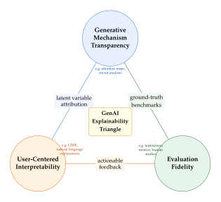
The GenAI Explainability Triangle
Generative models present a richer explainability surface than discriminative models. We organise the challenge using what we call the GenAI Explainability Triangle: three interrelated demands that must all be addressed for a generative system to be considered genuinely explainable.
Vertex 1: Generative Mechanism Transparency. What latent variables, attention patterns, or intermediate representations caused the specific output? For a language model this includes: which training documents are being implicitly recalled, which attention heads are routing information from which positions, and whether the model is “reasoning” or “pattern-matching” (to the extent that distinction is coherent). For a diffusion model it includes: which noise trajectory was taken, which guidance signals shaped the denoising path, and how the latent manifold was traversed.
Vertex 2: User-Centered Interpretability. What explanation is appropriate for a given user with a given need? A data scientist querying a language model needs a different explanation than a radiologist, a judge, or a patient. The explanation must be adapted to the user's domain model, the consequentiality of the decision, and the available interaction modality.
Vertex 3: Evaluation Fidelity. Can we measure whether an explanation is correct? For discriminative models, fidelity metrics like area under the perturbation curve (Samek et al., 2017) are well-established. For generative models, standard fidelity metrics are largely undefined because the ground truth causal mechanism is unknown and the output space is high-dimensional and structured.
Why Generative Models Are Harder to Interpret
Classical XAI was developed primarily for discriminative models: classifiers and regressors that map a fixed input to a scalar or low-dimensional output. Methods like LIME, SHAP, Grad-CAM (Selvaraju et al., 2017), and integrated gradients (Sundararajan et al., 2017) produce saliency maps or feature attributions that highlight which input features most influenced a particular classification.
Generative models introduce three qualitative difficulties that these methods do not address:
Stochastic sampling.
A discriminative model is typically deterministic given . A generative model samples from a distribution . Two forward passes with the same input and parameters can produce arbitrarily different outputs. An attribution method that computes gradients of the output with respect to the input is undefined or ambiguous for a stochastic output. Even if we fix the random seed, the attribution reflects that seed's trajectory, not the model's distributional behaviour.
High-dimensional, structured output spaces.
Discriminative model outputs are typically scalar or low-dimensional. Generative outputs are sequences of tokens, images with millions of pixels, audio waveforms, or protein structures. Attribution methods that assign a scalar importance score to each input feature face a fundamental mismatch: the output is not a scalar to differentiate with respect to. Extending gradient-based attributions to sequence outputs requires integrating over output positions, which introduces aggregation choices that interact poorly with long-range dependencies.
Multi-step generation.
Many generative models involve multiple cascaded components: a language model may use retrieval, chain-of-thought, a code interpreter, and post-processing. A diffusion model iterates hundreds of denoising steps through multiple network passes. A VAE encodes, samples, and decodes. Each intermediate step introduces its own representation, its own stochasticity, and its own opportunities for information to be created, discarded, or transformed. Attribution methods designed for single forward passes cannot natively attribute credit across such pipelines.
The following table summarises the qualitative differences in the XAI challenge between discriminative and generative models.
| XAI Dimension | Discriminative Models | Generative Models |
| Output type | Scalar / low-dimensional label | Sequence, image, audio, or structured object |
| Determinism | Deterministic given parameters | Stochastic; distribution over outputs |
| Attribution target | Single output scalar | Ambiguous: which token, pixel, or step? |
| Evaluation of attributions | Pixel-flipping, deletion curves | No standard metrics; output space too complex |
| Forward pass structure | Single encoder + head | Multi-stage pipeline; retrieval; sampling |
| Latent space | Compact class embeddings | High-dimensional, entangled; sampling noise |
| Causal question | Why this class? | Why this generation trajectory? |
| Human-facing utility | Highlight discriminative pixels | Identify failure modes, bias, copying |
| Faithfulness measurable? | Yes (deletion / perturbation) | Difficult; ground truth not available |
| Regulatory touchpoint | GDPR Article 22 | EU AI Act high-risk systems |
Key Idea.
The generative-discriminative interpretability gap. Understanding how a model generates is fundamentally different from understanding why it classifies. Classification can be explained by identifying which input features shift the output probability; the output itself is fixed (a class label) and the causal graph is shallow. Generation requires explaining the choice of an entire trajectory through a structured output space: every token, every denoising step, every attention pattern contributes to the final output in a way that cannot be reduced to a simple saliency score. The key challenge is trajectory attribution: assigning credit or blame across the joint space of inputs, latent variables, and multi-step outputs.
Biological Connections: Neural Coding and Distributed Representations
The question of how information is encoded in neural networks, artificial or biological, has a long history in neuroscience that illuminates the interpretability challenge. Two competing theories of neural coding have shaped the field.
The sparse coding hypothesis.
Barlow (1961) proposed that the nervous system achieves efficient representation by using as few neurons as possible to encode each stimulus. In the extreme, the grandmother cell hypothesis (Gross, 2002) posits that individual neurons represent specific high-level concepts: one neuron fires for your grandmother's face, one fires for Jennifer Aniston, one fires for the Eiffel Tower. This is trivially interpretable: if you can label each neuron, you can read off the model's internal representation.
Evidence for this view comes from the seminal work of Hubel and Wiesel (1959, 1962), who found neurons in primary visual cortex that respond selectively to oriented edges at specific spatial frequencies, and from Quiroga et al. (2005), who found neurons in the human medial temporal lobe responding to single specific individuals or landmarks.
The distributed representation hypothesis.
McCulloch and Pitts (1943) and later Hinton, McClelland, and Rumelhart (1986) argued for a fundamentally different coding scheme: information is represented by patterns of activity across many neurons, no single one of which is individually interpretable. A face is encoded as a high-dimensional activation vector, not as a single neuron's firing rate. This allows combinatorial generalisation: neurons can represent up to distinct patterns rather than concepts.
Modern deep neural networks clearly use distributed representations. This makes them powerful and difficult to interpret simultaneously. However, recent work in mechanistic interpretability suggests that superposition (Elhage et al., 2022) allows networks to store more features than dimensions by representing features as near-orthogonal directions in activation space, with small but non-zero interference.
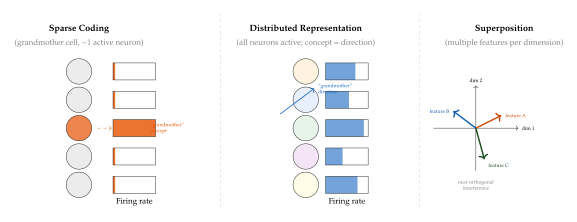
The superposition hypothesis has important implications for interpretability. If a network stores features in dimensions via superposition, then probing individual neurons is insufficient: the features are polysemantic (a single neuron responds to multiple unrelated concepts). Recovering individual features requires finding sparse decompositions of the activation space, which is the goal of sparse autoencoders in mechanistic interpretability (Cunningham et al., 2023; Bricken et al., 2023).
Example 1 (Polysemanticity in InceptionV1).
Olah et al. (2020) found that neuron 379 in the mixed3b layer of InceptionV1 responds maximally to images of: (i) cat faces, (ii) car fronts, and (iii) specific curved textures. These concepts appear unrelated from a human perspective, yet the network has learned to use the same neuron to represent them. This is not a flaw in the network's reasoning; it is the network efficiently packing information into constrained dimensional space via superposition. The interpretability challenge is to decompose this polysemantic response into monosemantic features.
Exercises
Exercise 1 (Transparency of Logistic Regression).
Let be a logistic regression classifier with parameter vector , bias , and the sigmoid function.
Show that is -transparent in the language of linear equations (Definition 1) by constructing an explicit description and verifying all three conditions.
Compute the SHAP values for this model and show they equal under the uniform background distribution (to first order).
Now consider a two-layer ReLU network . Explain why no description of sub-linear length in can faithfully capture all activation patterns, and hence why ReLU networks are not -transparent for in general.
Exercise 2 (Introspection Gap in Language Models).
Consider a language model that generates a chain-of-thought (CoT) rationale followed by an answer : for a question .
Define a formal notion of CoT faithfulness: the degree to which is causally responsible for vs. a post-hoc rationalisation. (Hint: use causal intervention notation for a different rationale .)
Turpin et al. (2023) showed that inserting a biasing hint into the context causes a model to change its answer but generate a rationale that does not mention the hint. Formalise this as a violation of your faithfulness criterion.
Propose an experimental protocol to measure faithfulness on a given question-answer dataset without access to the model's internal activations.
Exercise 3 (The Superposition Capacity Bound).
Elhage et al. (2022) show that neurons can represent features in superposition if the features are nearly orthogonal with pairwise interference .
Using the Johnson-Lindenstrauss lemma, show that one can embed unit vectors in with pairwise inner products at most , for an absolute constant (so the exponent is linear in ).
Argue that polysemanticity is an inevitable consequence of representing many features in low-dimensional spaces, not a design flaw. What does this imply for the viability of neuron-level interpretability?
Describe how sparse autoencoders can in principle “un-mix” superposed features. What objective would you minimise, and what sparsity constraint would you impose?
The Mechanistic Interpretability Paradigm
Defining the Programme
Mechanistic interpretability is the programme of reverse-engineering trained neural networks into human-understandable computational processes. The goal is not to produce a local explanation for a single prediction (as in SHAP or LIME) but to produce a complete account of the algorithm a network has learned: which neurons compute which features, how those features are combined via attention or MLP operations, and what high-level algorithm the resulting circuit implements.
Definition 4 (Mechanistic Interpretability).
Given a trained neural network and a behaviour (a function from inputs to outputs that exhibits on some distribution), a mechanistic explanation of is a tuple where:
is a circuit: a sub-graph of the computation graph of ,
is an interpretation map assigning human-meaningful algorithms to nodes in ,
is a fidelity metric satisfying on the behaviour distribution, where is with all non- components ablated.
The explanation is complete if ; it is -faithful otherwise.
Insight.
Mechanistic interpretability is to AI what molecular biology is to medicine. Classical pharmacology observed that certain substances produced clinical effects, but could not predict new drugs without understanding the molecular mechanisms. Molecular biology's account of protein structure, enzyme kinetics, and receptor binding turned pharmacology into a science capable of rational drug design. Similarly, current deep learning is largely correlational: we observe what networks can do on benchmarks, but cannot predict failure modes, design interventions, or transfer knowledge systematically without a mechanistic account. Mechanistic interpretability aims to provide that account.
Three Abstraction Layers
The mechanistic interpretability programme operates at three interrelated levels of abstraction, inspired by Marr's three levels of analysis in computational neuroscience (Marr, 1982).
Layer 1: Neurons as Features.
At the finest grain, individual neurons (or directions in activation space) represent specific features of the input. For vision models these may be edge detectors, colour blobs, or object part detectors. For language models they may represent syntactic roles, entity types, or factual properties. The goal at this layer is to produce a feature dictionary: a mapping from neurons (or sparse directions) to their semantic content.
Methods at this layer include:
Maximum activation examples: find the training or held-out inputs that maximally activate a neuron, and infer the feature from the pattern.
Activation patching on concepts: verify that a neuron represents a concept by measuring the downstream effect of setting its activation to its mean.
Sparse autoencoders (SAEs): learn a sparse, overcomplete dictionary such that activations with . Each column of is a purported monosemantic feature.
Layer 2: Circuits.
A circuit is a sub-graph of the computation graph connecting features to downstream features through specific attention heads, MLP layers, or residual stream connections. Circuits explain specific input-output relationships: “the indirect object identification circuit in GPT-2 (Wang et al., 2022) routes the subject token's representation through three specific attention heads to generate the indirect object at the output position.”
The circuit paradigm was established by Olah et al. (2020) who reverse-engineered a curve-detector circuit in InceptionV1, showing that curve detector neurons receive inputs from oriented edge detector neurons (themselves identified as implementing a Fourier decomposition of local contrast patterns) via a specific set of connections. The insight that the same circuit type (curve from edges) recurs at multiple spatial positions is the notion of circuit universality: similar circuits emerge in different networks trained on different tasks, suggesting convergent algorithmic solutions.
Layer 3: Macroscopic Algorithms.
At the coarsest grain, what high-level algorithm does the network implement? For GPT-2 on the indirect object identification (IOI) task, Wang et al. (2022) showed the algorithm has three phases: (i) token copying, in which name mover heads copy subject representations to the final token position; (ii) subject suppression, in which inhibition heads downweight the current subject relative to alternatives; and (iii) output generation, in which name mover heads promote the correct output. This three-phase description is a macroscopic algorithm that could in principle be implemented differently by a different network, but which GPT-2 happened to implement through the specific circuit identified at Layer 2.
Remark 3.
Analogy with molecular biology. These three layers map onto biological levels of analysis: neurons as features molecular mechanisms (which protein does what function); circuits cellular pathways (how proteins interact in biochemical cascades); macroscopic algorithms physiological processes (how pathways produce tissue- or organ-level behaviour). The analogy is not perfect but is instructive for motivating the hierarchical programme.
The Causal Intervention Toolkit
Mechanistic interpretability relies on causal interventions: modifying specific activations in the network and observing the downstream effect. This section formalises the four main techniques.
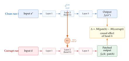
Let be a transformer with layers, attention heads per layer, and hidden dimension . Denote by the attention head output of head in layer at position , and by the MLP output at layer , position . The residual stream at position after layer is: (Residual) where is the token embedding at position .
Definition 5 (Activation Patching).
Given a clean input and a corrupted input , the activation patch at component is the operation of running on while replacing the activation with the clean value from the run on . The patching effect is: (Actpatch) where is a scalar metric (e.g., logit difference of target tokens). A large positive indicates that head at position is causally responsible for the correct behaviour on .
Definition 6 (Path Patching).
Path patching (Wang et al., 2022; Goldowsky-Dill et al., 2023) extends activation patching by patching not just a component's output but the path from a source node to a target node through a specific intermediate set . Formally, let be the computation graph. For a path with , path patching intervenes on the value that receives from : (Pathpatch) Path patching is strictly more precise than activation patching because it isolates the information flow through a specific causal path rather than replacing all information passing through a node.
Definition 7 (Mean Ablation).
Mean ablation of component replaces the component's activation with its mean over a reference distribution : (Meanablation) Mean ablation removes the component's contribution to the specific input while retaining the average contribution from the reference distribution. It is less disruptive than zero ablation (which sets activations to zero, a potentially out-of-distribution value) but conflates information from multiple inputs.
Definition 8 (Resampling Ablation).
Resampling ablation (also called activation resampling) replaces the activation at with the value from a randomly sampled corrupted input that has a different label or target than : (Resample) and measures . Resampling ablation preserves the statistical properties of the activation distribution, avoiding the out-of-distribution problem of zero ablation.
Automated Circuit Discovery
Manual circuit analysis (Olah et al., 2020; Wang et al., 2022) requires a researcher to form and test hypotheses about each attention head and MLP component. For GPT-2-small (117M parameters, 12 layers, 12 heads per layer), this process required several months of researcher time per circuit. For modern large language models the brute-force approach is computationally and cognitively intractable.
Two algorithmic approaches have emerged to automate circuit discovery.
ACDC (Automated Circuit DisCovery).
Conmy et al. (2023) introduce ACDC, a greedy top-down algorithm that identifies the minimal sub-graph of the computation graph sufficient to reproduce a target metric. Starting from the full computation graph, ACDC iteratively ablates edges (connections between components) and retains an edge if its ablation causes the metric to change by more than a threshold : (ACDC) The output is a minimal circuit such that all retained edges contribute more than to the metric. ACDC is correct by construction for greedy selection but may miss non-minimal circuits that interact synergistically.
Edge Attribution Patching (EAP).
Syed et al. (2023) and Marks et al. (2024) propose EAP as a gradient-based approximation to path patching that scales to large models. For each edge in the computation graph, EAP computes an attribution score: (EAP) where is the residual stream at on the corrupted input and is the same on the clean input. The gradient is computed with a single backward pass on the clean input. EAP thus requires only two forward passes (clean and corrupt) and one backward pass, regardless of circuit size.
The key insight is that approximates the first-order contribution of restoring the clean activation at via edge to the metric. The approximation is exact in the linear limit and remains accurate when activations are small perturbations of their clean values.
Proposition 1 (Computational Complexity of Circuit Discovery).
Let be a transformer with layers, heads per layer, and token positions. The computation graph has edges (each head at each layer-position pair can attend to each previous layer-position pair).
Brute-force activation patching requires forward passes, one per component: passes total if patching individual head outputs (not all edges), or passes for all edges.
ACDC requires forward passes in the worst case (one ablation test per edge) but converges in practice to passes for a circuit of retained edges, since it prunes iteratively.
EAP requires forward passes (two forward + one backward), independent of . The approximation error is per edge, which is small when clean and corrupt inputs are close.
Proof.
Part (a) follows directly from counting the number of components. For layers, heads, and positions, there are head-position pairs; patching each requires one forward pass. For all edges in the computation graph, all edges must be tested.
Part (b): ACDC starts with the full graph and greedily removes edges. At each step it needs to evaluate one edge ablation per remaining edge. In the worst case (no edges removed), this is passes. In practice, after pruning rounds the circuit shrinks geometrically.
Part (c): EAP uses a first-order Taylor expansion. The attribution for edge uses evaluated once on the clean input (one backward pass) and the activation difference from two forward passes. The error per edge is bounded by the second-order term, which is , completing the proof.
A Taxonomy of Mechanistic Interpretability Methods
| Method | Layer | Core Technique | Key Reference | Cost |
| Max activation examples | Neuron | Find inputs maximising neuron firing | Olah et al., 2017 | |
| Feature visualisation | Neuron | Gradient ascent in input space | Olah et al., 2017 | |
| Probing classifiers | Neuron | Train linear probe on activations | Alain & Bengio, 2017 | |
| Sparse autoencoders | Neuron | Learn overcomplete sparse basis | Bricken et al., 2023 | |
| Logit lens | Neuron/Circuit | Project intermediate states to logits | Nostalgebraist, 2020 | |
| Activation patching | Circuit | Restore clean activations selectively | Meng et al., 2022 | |
| Path patching | Circuit | Patch specific computational paths | Wang et al., 2022 | |
| Mean ablation | Circuit | Replace with distributional mean | Chan et al., 2022 | |
| ACDC | Circuit | Greedy edge pruning via ablation | Conmy et al., 2023 | |
| EAP | Circuit | First-order gradient attribution | Syed et al., 2023 | |
| Causal tracing | Algorithm | Corrupt + restore; locate facts | Meng et al., 2022 | |
| ROME / MEMIT | Algorithm | Rank-one model editing | Meng et al., 2022/2023 | |
| Attention analysis | Algorithm | Visualise attention weight patterns | Clark et al., 2019 |
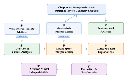
Chapter Roadmap
The remainder of this chapter develops the mechanistic interpretability programme for generative models specifically. Figure 4 shows the organisation.
Exercises
Exercise 4 (Implementing Activation Patching).
Consider a two-layer attention-only transformer with residual stream (token embeddings), two attention heads per layer, and a linear unembedding . The metric is the logit difference for a correct token and incorrect token .
Write the activation patching effect (Equation (Actpatch)) for this specific architecture. Simplify using the linearity of the residual stream.
Show that for linear attention (removing the softmax), activation patching is equivalent to computing the gradient of with respect to the head output and multiplying by the activation difference . (This is the theoretical basis for EAP.)
Describe the experimental design for the indirect object identification (IOI) task on a toy dataset: what are and , what is , and how would you interpret a heat-map of over all ?
Exercise 5 (Circuit Fidelity Metric).
Given a circuit in the sense of Definition 4, define the circuit fidelity as: (Fidelity) where is the model with all components outside mean-ablated, and is the model with all components mean-ablated.
Show that when is a probability and mean-ablation produces outputs in . Give a counterexample when is a logit difference.
Prove that and for any .
Define circuit minimality: is -minimal if and for every proper sub-circuit , . Show that finding an -minimal circuit is NP-hard in general (reduce from minimum vertex cover).
Exercise 6 (Mean Ablation vs. Zero Ablation).
Let be a single attention head with parameters .
Show that zero-ablating (setting its output to ) is equivalent to inserting an input for which . Argue this may be out-of-distribution in a network trained with non-zero random initialisation.
Let be the mean activation over a reference distribution. Show that mean-ablating is equivalent to adding a constant bias to the residual stream and subtracting the head's contribution. Derive an expression for this effective bias in terms of .
In a transformer with LayerNorm, mean activations may not be zero even for zero-mean inputs. Give a concrete example using the GPT-2 architecture where zero-ablation and mean-ablation of an attention head produce measurably different logit differences, and explain which should be preferred for causal inference and why.
Classical Explainability Methods
Before we can understand why interpretability for generative models demands fundamentally new tools, we must master the classical toolkit. The methods developed between 2016 and 2020 - SHAP, LIME, Grad-CAM, Integrated Gradients, and attention visualisation - represent the mature engineering of a particular idea: that a model's prediction on a given input can be explained by attributing credit or blame to the individual input features that drove it. These are attribution methods, and they are extraordinarily successful at what they do. They are also, as we shall argue in Why Classical XAI Fails for Generative Models, fundamentally inadequate for generative models.
The story of attribution methods begins with a question that seems almost embarrassingly simple. Given a neural network that classifies an input and produces a prediction , which features of were responsible? For a radiologist looking at a chest X-ray classified as showing pneumonia, this question is not academic: it determines whether the model can be trusted, whether it has learned the right visual patterns, and whether the radiologist's intuition aligns with the machine's. For a judge evaluating whether an algorithmic decision was fair, knowing which features drove the decision is a legal requirement in many jurisdictions.
Yet the question conceals a thicket of subtlety. What does it mean for a feature to be “responsible” for a prediction? Features are not independent; removing or perturbing one changes the context for all others. The model is a nonlinear function of thousands or millions of parameters, not a transparent formula one can inspect directly. And the very notion of feature importance is ambiguous: do we mean the feature's causal effect on the output, its correlation with the output, or some measure of counterfactual sensitivity?
The four methods we study in this section each answer this question differently, and their different answers reveal complementary facets of model behaviour.
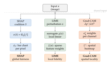
SHAP: Shapley Values from Game Theory
The most principled approach to attribution comes not from machine learning but from cooperative game theory. In 1953, Lloyd Shapley solved the problem of fairly distributing the proceeds of a cooperative game among its players, and his solution - now bearing his name - has become the mathematical foundation of modern feature attribution.
Cooperative Games and Fair Division
A cooperative game is a pair where is a set of players (here, feature indices) and is a characteristic function that assigns a real-valued payoff to every subset (coalition) . For attribution purposes, represents how well a model performs when only the features in are available. Typically, where and the expectation marginalises over all features not in , while features in retain their observed values.
The Shapley value of player measures that player's average marginal contribution across all possible orderings in which players join the coalition.
Definition 9 (Shapley Value).
Given a cooperative game with players, the Shapley value of player is (Shapley) The quantity is the marginal contribution of player to coalition . The prefactor is the probability that coalition forms before player joins, under a uniform random ordering of all players.
The Shapley value is the unique allocation satisfying four axioms that formalise the notion of fairness.
Theorem 1 (Shapley Axioms).
The Shapley value is the unique function satisfying all of the following:
Efficiency. . The attributions sum to the model's total output difference.
Symmetry. If for all , then . Interchangeable players receive equal attribution.
Dummy. If for all , then . A feature that never changes the output receives zero attribution.
Linearity. for any two games and scalars .
KernelSHAP: Tractable Approximation
Direct computation of Shapley values requires evaluating on all subsets, which is computationally infeasible for high-dimensional inputs. Lundberg and Lee (2017) introduced SHAP (SHapley Additive exPlanations), a practical framework with the KernelSHAP algorithm as its model-agnostic backbone.
The key observation is that Shapley values can be cast as the solution to a weighted least-squares problem. Define a coalition vector indicating which features are present, and let the SHAP kernel weight for coalition (encoded as ) be (Kernel) Then the SHAP attributions are obtained by solving (Kernelshap) where is the binary indicator of . In practice, one samples a manageable number of coalitions (typically ), evaluates on each (possibly by querying with missing features replaced by background samples), and solves the weighted least-squares problem.
Key Idea.
SHAP unifies several earlier attribution methods as special cases. TreeSHAP exploits tree structure for exact computation (where is the number of trees, is the maximum number of leaves, and is the maximum tree depth). DeepSHAP propagates SHAP values through neural network layers using the chain rule. LinearSHAP recovers exact Shapley values for linear models in closed form. The unifying principle is always the same: the Shapley value is the unique fair attribution that respects the axioms of efficiency, symmetry, dummy, and linearity.
LIME: Local Interpretable Model-Agnostic Explanations
While SHAP seeks a globally consistent attribution grounded in game theory, LIME (Ribeiro, Singh, and Guestrin, 2016) takes a pragmatically local approach: fit a simple interpretable model to the behaviour of the complex model in the neighbourhood of a specific input.
Local Surrogate Framework
Given an input and a black-box classifier , LIME constructs a local surrogate (typically a sparse linear model) that approximates near . The explanation is the solution to (LIME) where:
is the local fidelity loss, measuring how well mimics on perturbations of , weighted by proximity ;
is an exponential kernel assigning higher weight to perturbations closer to ;
is a complexity penalty (e.g., norm of the linear weights) that encourages sparse, human-readable explanations.
The perturbations are generated by randomly masking a subset of superpixels (for images) or words (for text), replacing masked regions with a background value or held-out tokens. The surrogate is then learned on the dataset using weighted ridge regression.
Locality and Its Implications
The locality of LIME's explanation is simultaneously its strength and its vulnerability. On the one hand, a local linear model can capture the local decision boundary of an arbitrarily complex classifier, provided the neighbourhood radius is calibrated correctly. On the other hand, different runs of LIME on the same input can produce qualitatively different explanations if the sampled perturbations happen to fall in different regions of a complex loss landscape. This instability is a documented limitation that has motivated several remediation strategies, including using larger perturbation budgets, fixing the random seed, and employing regularised regression in place of standard ridge.
Remark 4.
The instability of LIME can be measured formally: if and are two runs of LIME on the same input with different random seeds, their explanations may satisfy even for well-calibrated hyperparameters. This is not a bug in LIME but a consequence of the fact that local linear models have high variance in high-dimensional settings.
Grad-CAM: Gradient-Weighted Class Activation Mapping
SHAP and LIME are model-agnostic: they treat the classifier as a black box and probe it by varying inputs. Grad-CAM (Selvaraju et al., 2017) takes the opposite approach, exploiting the internal gradient structure of convolutional neural networks to produce spatial saliency maps that highlight where in the image the model looked when making its prediction.
Class Activation Maps via Gradients
Let denote the activation map of the -th feature map in the final convolutional layer, and let be the logit (pre-softmax score) for class . Grad-CAM computes the importance weight of the -th feature map for class by globally average-pooling the gradient of with respect to : (Weight) The Grad-CAM saliency map is then (MAP) where the ReLU discards negative contributions (features that suppress class ) and retains only the positive evidence. The resulting map is upsampled (bilinearly) to the input resolution and overlaid on the image.
The ReLU operation in (MAP) is a deliberate choice. Without it, the map would include features that suppress the predicted class, producing a noisier and harder-to-interpret visualisation. With it, Grad-CAM produces localised, high-contrast heatmaps that are easy for human experts to interpret.
Example 2 (Grad-CAM on a Medical Image Classifier).
Consider a ResNet-50 classifier trained to detect pneumonia from chest radiographs. Given a positive-class input (a radiograph classified as pneumonia), we apply Grad-CAM to visualise which spatial regions drove the prediction.
Setup. Let the final convolutional layer have feature maps of spatial resolution . The logit for the “pneumonia” class is . We compute the gradient via a single backward pass, average-pool to obtain , and form the weighted sum.
Result. The Grad-CAM heatmap localises to the right lower lobe of the lung, precisely where a radiologist would look for consolidation. The model's spatial attention is medically plausible, providing a first-pass validation that the network has learned clinically meaningful patterns rather than spurious correlations (e.g., orientation tags, scanner artefacts, or hospital watermarks).
Clinical utility. Beyond trust assessment, Grad-CAM maps can flag cases where the model attends to implausible regions - for instance, the diaphragm or cardiac silhouette in a lung-disease classifier - which may indicate dataset bias or distribution shift. At one large hospital system, routine Grad-CAM auditing of a pneumothorax detector revealed that of its “confident” predictions were driven by scanner metadata rather than lung parenchyma; retraining on a cleaned dataset reduced this to .
Limitations. Grad-CAM is coarse (limited by the spatial resolution of the last convolutional layer) and class-specific but not instance-specific: two different images of the same class may produce similar heatmaps even if the discriminating features differ. Grad-CAM++ and Score-CAM address some of these limitations by using second-order gradients and activation-based weighting, respectively.
Integrated Gradients: Path-Based Attribution with Axioms
Integrated Gradients (Sundararajan, Taly, and Yan, 2017) sits at a conceptual crossroads between the game-theoretic rigour of SHAP and the gradient efficiency of Grad-CAM. Like SHAP, it is grounded in a set of formal axioms; like Grad-CAM, it exploits the gradient of the network with respect to its input. Unlike Grad-CAM, it is architecture-agnostic: it applies to any differentiable model, not just convolutional networks.
Path Integral and Axiomatic Foundation
The Integrated Gradients attribution of feature is defined as the integral of the gradient along a straight-line path from a baseline (representing “no signal”, e.g. an all-black image or an all-padding text sequence) to the actual input : (IG) In practice, the integral is approximated by a Riemann sum over equally-spaced steps along the path: (Approx) For this right-endpoint Riemann sum the approximation error decreases as (a midpoint or trapezoidal quadrature would improve this to ); values of are standard in practice.
Theorem 2 (Axiomatic Characterisation of Integrated Gradients).
Integrated Gradients is the unique path method satisfying all of the following axioms:
Completeness. . The attributions sum exactly to the output difference between the input and the baseline. This is the analogue of SHAP's Efficiency axiom.
Sensitivity. If and and differ in only one feature , then . A feature that changes the output must receive non-zero attribution.
Implementation Invariance. Two functionally equivalent networks (same input-output mapping, different architectures) produce identical Integrated Gradients attributions.
Linearity. For networks and scalars : .
Symmetry-Preserving. If is symmetric in features and , then .
Among all attribution methods satisfying Sensitivity and Implementation Invariance, Integrated Gradients uniquely satisfies Completeness.
The Completeness axiom is particularly important from an auditing perspective: it guarantees that the explanation accounts for the entire prediction, with no attribution budget left unaccounted for. By contrast, vanilla gradient-times-input methods (which multiply the gradient at by the input value) can violate Completeness because they do not integrate over the path.
Attention Visualisation: Is Attention Explanation?
The rise of Transformer models introduced a new form of “explanation” that is appealing in its simplicity: attention weights. When a text classifier based on BERT produces a prediction, the multi-head self-attention layers produce weight matrices (one per head per layer) that ostensibly indicate how much each token “attends to” every other token. Visualising these weights as heatmaps became a popular way to explain model behaviour, and several major NLP papers in 2018–2019 relied on attention visualisations to support interpretability claims.
The Jain-and-Wallace Challenge
In a landmark 2019 paper, Jain and Wallace challenged the assumption that attention weights constitute valid explanations. Their argument rests on two empirical observations and one theoretical argument.
Empirical finding 1: Attention and feature importance disagree. When LIME and gradient-based attributions are computed alongside attention weights for the same prediction, the resulting attributions are poorly correlated (Spearman in many cases). High attention weight on a token does not imply that token drives the prediction.
Empirical finding 2: Adversarial attention. It is possible to construct “adversarial attention” distributions that produce the same model output as the original attention distribution while being maximally different in the attention weights. Formally, given a prediction produced with attention , Jain and Wallace find an alternative attention such that but is large. This demonstrates that the mapping from attention to output is many-to-one: attention can be changed dramatically without changing the prediction.
Theoretical argument: Attention is an intermediate computation. Attention weights are computed inside the model, not at the interface between model and input. They capture which token representations are mixed at a given layer, but the final prediction depends on how those mixed representations are subsequently processed by feed-forward sublayers, layer normalisation, and additional attention heads. Attributing the prediction to attention weights at one layer ignores all downstream processing.
Caution.
Attention is Not Explanation.
Visualising attention weights as explanations conflates a model's internal routing mechanism with the causal attribution of output to input. Specifically:
High attention weight on a token does not imply that removing would change the prediction (violation of the Sensitivity axiom).
Attention weights do not satisfy Completeness: they do not sum to the output value.
In multi-head attention, different heads may attend to the same token for entirely different reasons; averaging across heads destroys this structure.
In deep Transformers, early-layer attention may track surface syntactic features while later-layer attention captures semantic relationships; mixing layers conflates these signals.
The controversy remains active. Wiegreffe and Pinter (2019) rebutted Jain and Wallace's adversarial construction, arguing that their adversarial attention distributions are not realisable without changing the value vectors, effectively changing the model itself. The current consensus is nuanced: attention can provide useful diagnostic signals but does not constitute a faithful, complete, or sensitive attribution in the formal sense required for trustworthy explanation.
What Attention Does Tell Us
Despite these limitations, attention visualisation is not worthless. Attention patterns in pre-trained language models exhibit systematic behaviours that are genuinely informative:
Syntactic heads. Certain heads in BERT's lower layers reliably attend along syntactic dependency arcs (subject-verb, noun-modifier), even though the model was never trained with syntactic supervision.
Coreference heads. Some heads track coreference chains, attending from pronouns to their antecedents.
Positional heads. A subset of heads implement diagonal attention (attending to the immediately preceding or following token), implementing a form of local context integration.
These patterns reveal something real about what the model has learned, even if they do not constitute faithful attribution of any specific prediction. The distinction matters: attention is a useful diagnostic tool for understanding model behaviour at the population level, but a poor explanatory tool for understanding any specific prediction.
Exercises: Classical Explainability Methods
Exercise 7.
(Shapley value computation.) Consider a binary classification model with three binary features . The model's outputs on all eight possible inputs are: Using the background value , compute the Shapley values for the input via (Shapley). Verify the Efficiency axiom: .
Exercise 8.
(Baseline sensitivity in Integrated Gradients.) Let be defined by (a scalar model for simplicity). Compute the Integrated Gradients attribution for input and each of the following baselines: (a) , (b) , (c) . Verify Completeness in each case. Discuss: for which baseline does the attribution most naturally correspond to the “importance” of the input relative to a natural reference point?
Exercise 9.
(Grad-CAM and the Sensitivity axiom.) Show by construction that Grad-CAM can violate the Sensitivity axiom of Integrated Gradients. Specifically, construct a two-layer ReLU network and an input such that , the prediction changes if feature is zeroed out, yet the Grad-CAM score for feature is zero. Hint: consider a network where the gradient at happens to be zero for due to ReLU saturation, even though the path integral is non-zero.
Why Classical XAI Fails for Generative Models
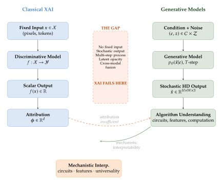
Classical XAI methods are engineered solutions to a specific problem: given a discriminative model (a classifier or regressor) and a fixed input , attribute the scalar prediction to the input features. The problem is well-posed: the input is fixed, the output is a scalar, and the attribution is a vector in . The methods we surveyed in Classical Explainability Methods are mature, principled, and - within their domain - genuinely useful.
The problem is that generative models are not discriminative models. A diffusion model, an autoregressive language model, a VAE, or a vision-language model does not classify an input; it produces outputs. And the production process is qualitatively different from classification in ways that systematically defeat every classical XAI method. This section catalogues these failure modes precisely, building toward the formal definition of what interpretability should mean for generative models.
The detective analogy is helpful here. Classical XAI assumes that we are trying to understand a judge's verdict: given the evidence (input ), which pieces of evidence drove the verdict ()? But a generative model is not a judge passing a verdict; it is a novelist writing a story. The novelist does not declare a fact; they generate a narrative that could have gone in many directions. Understanding the novelist requires a fundamentally different set of questions: What algorithms does the novelist employ? What internal representations mediate the creative process? How does the initial prompt constrain the space of possible stories?
The Attribution Problem: What Is the Input?
All classical XAI methods presuppose a fixed, well-defined input to which attributions are assigned. For a ResNet classifying an image, is a pixel tensor; for a BERT model classifying sentiment, is a token sequence. The attribution vector is indexed by the same dimensions as .
Generative models confound this assumption in several distinct ways.
The condition vs. the generation.
In a conditional generative model such as a text-conditioned image diffusion model, the input comprises both the condition (the text prompt) and the noise seed (the initial Gaussian sample that seeds the reverse process). If a generated image contains a spurious artefact, is it attributable to or ? The artefact may arise from the interaction of specific prompt tokens with specific noise configurations in ways that cannot be decomposed.
Unconditional generation.
In unconditional models (vanilla VAEs, vanilla GANs, unconditional diffusion), there is no condition at all. The “input” is pure noise , which has no semantic meaning. Attributing a generated face's eye colour to specific dimensions of is technically feasible (one can compute ) but semantically meaningless without a prior understanding of what represents - and that understanding is precisely what is missing.
The prompt is not the cause.
In large language models, the prompt is the nominal input, but the model's generation also depends on its entire training history (encoded in ), the decoding algorithm (temperature, top-, beam search), and - in stochastic decoding - the random seed. Attributing a specific generated sentence to specific prompt tokens conflates these three qualitatively different sources of influence.
Key Idea.
For discriminative models, the input is a fixed observation and the output is a deterministic function of it (modulo implementation randomness). For generative models, the “input” is a composite of semantic condition , noise seed , model parameters , and decoding hyperparameters . No single element is privileged as “the input”, and attributing output properties to any one element ignores the others.
Stochastic Generation: Same Input, Different Outputs
Classical XAI methods implicitly assume that is a deterministic scalar. LIME builds a local surrogate by querying on perturbations of and recording the outputs; SHAP evaluates ; Grad-CAM computes . All of these operations require either a deterministic output or the ability to marginalise over randomness in a controlled way.
Generative models are stochastic by design. A diffusion model with temperature produces a different image on every forward pass for the same prompt. An autoregressive model with nucleus sampling generates a different completion on every call. A VAE samples and decodes , with two stochastic steps.
This stochasticity creates a fundamental problem for attribution.
Which output do we explain?
Given stochastic outputs from the same prompt, LIME would need to construct a different surrogate for each output (since each has different pixel values to be attributed). Averaging the surrogates loses information about which outputs are typical and which are outliers. Explaining the average output is misleading because the average is itself not a typical output of the generative model (it is blurry, for diffusion models, or incoherent, for language models).
Output variance as information.
The variance across stochastic outputs is itself a meaningful signal: high variance indicates that the model is uncertain or that the prompt under-specifies the generation. Classical XAI methods entirely ignore this variance, providing no tools to explain why the model is uncertain or which prompt tokens are responsible for under-specification.
Remark 5.
Formally, for a stochastic generative model , the SHAP efficiency axiom requires attributions to sum to a scalar. If the target quantity is the marginal probability of a specific output , i.e., , then SHAP attributions assign credit to prompt tokens for explaining the log-likelihood of a specific sample. But this quantity depends on both and jointly, and a different yields a completely different attribution vector. There is no canonical choice of “the output” over which to compute attributions.
Multi-Step Processes: The Attribution Chain Problem
Diffusion models generate through denoising steps. Autoregressive language models generate through sequential token predictions, where may be hundreds or thousands. In both cases, the final output is the result of a long chain of stochastic transformations, and the causal structure of this chain creates fundamental obstacles for classical attribution.
Diffusion: The T-Step Attribution Puzzle
In a DDPM with steps, the generation proceeds as a Markov chain: where each step applies the learned denoising network . If we wish to attribute a feature of the final image (say, the presence of a red object in the upper-left quadrant) to the initial noise , we must trace the causal path through all denoising steps.
A single application of Grad-CAM at the final denoising step provides a saliency map for the last step, but ignores the contributions of steps . The contribution of early steps is mediated through the intermediate states , which are never observed (in standard sampling) and whose dimensions lack semantic meaning.
Integrated Gradients can in principle be applied by treating as the input and defining a baseline (e.g., the zero vector). But the straight-line interpolation from to passes through intermediate noise tensors that are not valid inputs to the denoising chain: the denoising network at step expects , not an arbitrary interpolation.
Autoregressive Models: The Token Dependency Graph
In an autoregressive language model, token is generated conditioned on all previous tokens , which include both the original prompt and the model's own previous generations. The causal graph of influences is a directed acyclic graph where every prompt token and every previously generated token can influence every future token.
SHAP can compute attributions for any specific output token by treating as the features. But the attributions change for every output token, and aggregating them across a multi-token generation requires a choice: sum? max? mean? Each aggregation discards structural information about how attribution evolves as generation proceeds.
Moreover, in teacher-forcing training, the model predicts each token conditioned on the ground-truth context, but in inference, it conditions on its own (possibly erroneous) previous predictions. Attributing a generation error to a specific prompt token may be misleading if the error was actually caused by an earlier generation error that snowballed.
Latent Space Opacity: VAE and GAN Codes
In discriminative models, the input has a natural human interpretation: pixels have positions, words have meanings. This semantic grounding is what makes feature attribution meaningful: saying “the model attended to the top-right corner” or “the word `not' had negative attribution” conveys actionable information.
Latent variable models fundamentally lack this semantic grounding.
VAE Latent Codes
In a VAE, the encoder maps an input to a distribution over a -dimensional latent space. The decoder maps latent codes back to data space. If we attribute a generated image feature to latent dimensions , what does this mean semantically?
In general, nothing. The latent code is organised by the ELBO objective to maximise reconstruction quality and keep the posterior close to the prior . There is no mechanism that ensures corresponds to any human-interpretable concept (“hair colour”, “facial expression”, “object shape”). In practice, latent dimensions in vanilla VAEs are entangled: may partially encode hair colour, face orientation, and background brightness simultaneously.
Disentanglement methods (-VAE, FactorVAE, TC-VAE) seek to encourage axis-aligned latent factors that correspond to independent generative factors. But even successful disentanglement does not guarantee semantic alignment: a disentangled latent code where controls “size of the leftmost object” and controls “hue of the background” may be interpretable by reference to the images but does not correspond to human-level concepts.
GAN Latent Spaces
In a GAN, the generator maps a noise vector to a data point. Unlike VAEs, GANs impose no constraint on the structure of : the latent space can be geometrically complex, with no guarantee of linearity, convexity, or semantic regularity.
GANSpace (Härkönen et al., 2020) and InterfaceGAN (Shen et al., 2020) discovered empirically that GAN latent spaces often contain interpretable directions: a vector such that traversing corresponds to a semantically coherent change in the generated image (e.g., ageing, adding glasses, changing hairstyle). But these directions must be discovered by post-hoc linear probing or supervised steering - they are not intrinsic to the latent code's native coordinates.
Remark 6.
The opacity of latent spaces creates a semantic grounding gap: classical XAI methods attribute model outputs to input features that have pre-existing human interpretations (pixels, words, superpixels). For generative latent variable models, there is no canonical human interpretation of the features being attributed to. Attributing a generated artefact to conveys no actionable information without a separately learned semantic dictionary for the latent space.
Cross-Modal Alignment: VLMs and the Fusion Problem
Vision-language models (VLMs) such as CLIP, DALL-E, Stable Diffusion, and GPT-4V add a further layer of complexity: they must fuse information from two qualitatively different modalities - visual tokens and text tokens - into a unified representation that drives generation. The alignment between modalities is learned implicitly through massive-scale contrastive or generative training, and the resulting representations are highly non-transparent.
The Cross-Attention Attribution Problem
In a latent diffusion model conditioned on text, cross-attention layers compute attention between visual tokens (keys and values from the spatial feature map) and text tokens (queries from the CLIP text encoder). The cross-attention weight measures the degree to which spatial position of the image attends to text token .
Visualising cross-attention maps (as in Prompt-to-Prompt and Attend-and-Excite) provides a form of spatial-textual attribution: “the word `sunset' drove the redness of the sky region.” But this attribution has the same problems as standard attention visualisation (see Attention Visualisation: Is Attention Explanation?) compounded by cross-modal entanglement: text tokens are processed by CLIP, which itself is a complex non-transparent model; visual tokens are extracted by a VAE encoder; and the cross-attention operates in a compressed latent space, not in pixel space.
Modality Attribution Failure
Consider the question: “In a CLIP-guided diffusion model that generated an image of a dog on a skateboard, how much of the `skateboard' visual content is attributable to the text prompt, how much to the image prior learned during training, and how much to the initial noise seed?” This question is natural for a human engineer debugging a generation failure, but it has no well-defined answer in the framework of classical attribution:
The text prompt provides the semantic intent (skateboard).
The model's weights encode the visual prior (what skateboards look like in the training distribution).
The noise seed determines which specific visual configuration is selected from the prior.
The CLIP text encoder transforms the word “skateboard” into a 512-dimensional vector whose relationship to the skateboard's visual appearance is encoded in the weights, not in any human-readable form.
Attributing the skateboard's visual presence to “the word `skateboard' in the prompt” conflates all of these factors. Classical SHAP over the text tokens would assign attribution to the word “skateboard” simply because removing it changes the output - but it would assign zero attribution to the training data that taught the model what skateboards look like, and zero attribution to the model architecture that determines how text and image representations are aligned.
The Fundamental Shift: From Feature Attribution to Algorithm Understanding
The failure modes catalogued above are not engineering deficiencies that can be patched by better implementations of SHAP or Integrated Gradients. They reflect a fundamental mismatch between the question that classical XAI asks and the question that generative model interpretability requires.
Classical XAI asks: which input features drove this output? This question presupposes a fixed input, a scalar (or low-dimensional) output, and a model that computes a deterministic function of the input. Generative models violate all three presuppositions.
Key Idea.
Classical XAI asks “which input features matter?” - a question appropriate for discriminative models where inputs have semantic meaning and outputs are scalar decisions. For generative models, which lack fixed inputs, produce stochastic high-dimensional outputs through multi-step algorithms, and encode knowledge in latent spaces with no inherent semantic grounding, we must ask a different question: “What algorithm does the network implement?”
This shift from attribution to algorithm understanding defines the programme of mechanistic interpretability: reverse engineering the computational primitives, circuits, and representations that a generative model uses to produce its outputs.
The shift has a precedent in the history of science. Early pharmacologists asked “which molecules in this extract reduce fever?” - an attribution question. Modern molecular pharmacology asks “what receptor does aspirin bind, and how does binding inhibit prostaglandin synthesis?” - a mechanistic question. The mechanistic question is harder to answer but provides qualitatively different understanding: it explains not just what works but why it works, and it enables prediction and design rather than mere post-hoc explanation.
A Taxonomy of Classical XAI Failure Modes
| Method | Autoregressive LM | Diffusion Model | VAE/GAN | VLM |
| SHAP | Partial: per-token | Critical: -step | Critical: latent | Critical: |
| attribution only | coalition eval | space opacity | cross-modal | |
| ignores generation | intractable | undef. input | entanglement | |
| LIME | Partial: prompt | Critical: no | Critical: no | Partial: prompt |
| perturbations | stable output | input to | perturbations | |
| only | to regress on | perturb | only; cross- | |
| attn ignored | ||||
| Grad-CAM | N/A: no | Partial: applies | N/A: no | Partial: cross- |
| conv. layers | at single step | conv. stack | attn maps are | |
| only | not Grad-CAM | |||
| Integr. Grads | Partial: per- | Critical: path | Partial: input | Critical: no |
| token only; | not in data | is latent; | semantic | |
| aggregation ad hoc | manifold | no semantics | baseline exists | |
| Attention | Misleading: | Misleading: | N/A | Misleading: |
| Viz. | not faithful | cross-attn | cross-modal | |
| attribution | partial only | attn conflated |
Interpretability Desiderata for Generative Models
Having identified the failure modes of classical XAI, we can now state positively what a satisfactory interpretability method for generative models must achieve. We formulate this as three formal desiderata.
Definition 10 (Interpretability Desiderata for Generative Models).
Let be a generative model with parameters , condition , and output distribution over . An interpretability method produces an explanation . We say is satisfactory if satisfies all three of the following desiderata:
Faithfulness. The explanation must accurately describe the computational process by which generates . Formally, let be the model behaviour predicted by , and let measure the divergence between the true model and the model as described by . Then is faithful if for some tolerance . An explanation that describes a plausible-sounding process that the model does not actually implement is not faithful, regardless of how interpretable it is to a human reader.
Completeness. The explanation must account for all components of the model's generative capacity that are relevant to the outputs being explained. Formally, if has identifiable properties (e.g., the presence of a specific object, the colour of a region, the sentiment of a sentence), then must provide an account for each in terms of identifiable model computations. An explanation that accounts for only a subset of the output's properties is incomplete.
Minimality. Among all faithful and complete explanations, should be the simplest: it should identify the smallest subset of model components (circuits, attention heads, MLP neurons, latent dimensions) whose behaviour is sufficient to account for the explained outputs. Formally, if is another faithful, complete explanation with fewer components than , then should prefer . Minimality is the Occam's razor of interpretability: it guards against over-explanation that attributes outputs to the entire model.
These desiderata generalise and extend the axiomatic foundations of classical XAI. Faithfulness generalises the Sensitivity axiom: both require that explanations accurately reflect causal relationships. Completeness generalises the Efficiency axiom of SHAP: both require that the explanation accounts for the total output. Minimality is new: it has no direct classical counterpart, because attribution methods over a fixed input space are automatically minimal (they produce exactly attribution values, one per feature). For generative models, where the explanation space is the set of computational circuits in the model, minimality is non-trivial to enforce.
Proposition 2 (Impossibility of Classical Faithfulness).
Let be any classifier and any attribution vector. For a generative model where the output space is high-dimensional and stochastic, there exists no attribution vector satisfying all three desiderata simultaneously under the constraint that the explanation is indexed by condition features alone.
Proof.
We sketch the argument. Faithfulness requires that accurately describes the generative computation. The generative computation involves both the condition and the model parameters ; any explanation indexed only by cannot be faithful to the model's internal algorithm (which depends on ). Completeness requires accounting for all output properties; since outputs are stochastic, any complete explanation must account for the model's uncertainty, which is a function of and jointly. No vector can encode both the condition-specific attribution and the model-parameter-encoded prior simultaneously without violating either faithfulness or completeness.
The proposition is not a counsel of despair. It identifies the correct unit of analysis: rather than attributing outputs to input features, interpretability methods for generative models must attribute outputs to model components (circuits, layers, attention heads, neurons, latent directions). This is the programme of mechanistic interpretability, which we develop in the subsequent sections of this chapter.
Historical Note.
The limitations of feature attribution methods were recognised early in the history of XAI. As early as 2017, Rudin (later to publish the influential “Stop Explaining Black Box Machine Learning Models for High Stakes Decisions” in 2019) argued that post-hoc explanations of opaque models provide false confidence: they explain a proxy of the model, not the model itself. The critique became sharper with the rise of large generative models. In 2022, the DALL-E 2 model card from OpenAI explicitly acknowledged that “attribution of generated content to training data is not yet a solved problem.” The European Union's AI Act (2024) includes specific provisions for “high-risk AI systems” that require interpretability, but notably exempts generative AI from the strictest attribution requirements, implicitly acknowledging that current methods cannot satisfy them.
The formal treatment of interpretability desiderata for generative models has been developed by several groups since 2022, including work at DeepMind on mechanistic interpretability of language models, Anthropic's research on feature superposition and circuit analysis in transformer models, and the MATS (ML Alignment and Theory Scholars) research programme. The desiderata in Definition 10 synthesise threads from this literature into a single formal framework.
Exercises: Failures of Classical XAI
Exercise 10.
(LIME under stochastic generation.) Suppose you attempt to apply LIME to a text-to-image diffusion model with denoising steps. You generate perturbations of the prompt “a red apple on a wooden table” by randomly masking words, and for each perturbation, you run the full diffusion sampling to produce an image. Define the LIME target as the average RGB value of the centre pixel of the generated image.
(a) Show that the expected variance of the LIME target across runs with the same perturbation (different noise seeds) can be larger than the variance across different perturbations (same noise seed), depending on the temperature parameter . Specifically, give a bound on the signal-to-noise ratio of the LIME regression as a function of (variance due to stochasticity) and (variance due to prompt masking).
(b) Propose and justify a modification to the LIME procedure that controls for noise-seed variance by fixing the seed across all perturbations. What new assumption does this modification introduce, and when is it violated?
Exercise 11.
(SHAP attribution for a VAE: the semantic grounding problem.) Consider a VAE with encoder (Gaussian with diagonal covariance) and decoder trained on face images. We wish to apply SHAP to explain why a specific decoded image has blue eyes, where is a sampled latent code.
(a) Define a characteristic function where measures the “blueness” of the decoded image when latent features in retain their values from and features in are marginalised by integration against the prior. Write out formally.
(b) Show that the SHAP attributions computed from this may assign high attribution to a latent dimension even if has no semantic relationship to eye colour, as long as it is statistically correlated with eye-colour-encoding dimensions through the prior . Provide a construction.
(c) Argue that the Efficiency axiom is satisfied but the explanation is not faithful in the sense of Definition 10.
Exercise 12.
(Testing the desiderata.) For each of the following putative explanations of a generative model, determine which of the three desiderata (Faithfulness, Completeness, Minimality) are satisfied and which are violated. Justify each answer.
(a) “The diffusion model generated a dog because the word `dog' was present in the prompt.” (Assume the explanation is obtained by SHAP over prompt tokens, fixing the noise seed.)
(b) “The image was generated by iteratively applying the learned denoising network for , starting from Gaussian noise .” (This is a complete description of the sampling algorithm.)
(c) “Attention head 14 in layer 8 of the U-Net implements an edge-detection circuit that activates on high-frequency spatial features and drives the sharpening of object boundaries in the final step of denoising.” (Assume this is verified by causal intervention experiments.)
The Mathematical Framework of Transformer Circuits
Modern large language models are, at heart, transformers: architectures built from repeated blocks of multi-head self-attention and feedforward networks connected by residual streams. To truly interpret what these models compute, we need more than visualisations of attention weights; we need a rigorous mathematical language for decomposing the computation into atomic, understandable units. This language is the theory of transformer circuits, developed by Anthropic researchers Elhage et al. as a precise mechanistic account of what individual components of a transformer compute and how they interact.
The central insight is beautifully simple: at every layer, each token maintains a vector called its residual stream, which acts as a shared communication bus. Every component-attention heads and MLP layers alike-reads from this bus, performs a transformation, and writes back an additive update. Because all operations are additive, the residual stream at any layer is an exact linear superposition of all previous contributions. This linearity is not an approximation; it is an architectural fact that makes the transformer uniquely amenable to circuit-level analysis.
The Residual Stream as a Communication Bus
We begin with a precise definition.
Definition 11 (Residual Stream).
Let denote the embedding of token produced by the embedding matrix applied to the one-hot token vector, plus a positional encoding. For a transformer with layers, each containing attention heads and an MLP sub-layer, the residual stream at layer for token is the vector (DEF) where is the total additive update contributed by layer (summing over all attention heads in that layer plus the MLP block). The logit for predicting vocabulary item after the final layer is (Final) where is the unembedding matrix.
The key structural consequence of (DEF) is that every component of the network interacts with every other component only through the residual stream. There are no direct skip connections between layer 1's attention heads and layer 3's MLP; the only path is through sequential reads and writes to the shared bus.
Token embedding .
The embedding matrix maps a discrete token index to a dense vector , where is the -th standard basis vector. In practice, the model learns end-to-end, and its columns are the token embedding vectors. The initialisation of the residual stream is (INIT) where is the positional encoding for position .
Unembedding .
The unembedding matrix maps the final residual stream vector back to logits over the vocabulary. In many implementations, (weight tying), although this is not universal in large models. The pre-softmax logit for token is , and the predicted probability is .
Remark 7.
The logit is a bilinear form in the final residual stream and the unembedding direction for token . Because the residual stream is a sum of contributions from all layers and heads ((DEF)), we can decompose the logit linearly over components. This logit attribution is the foundation of the logit lens technique in The Logit Lens: Tracking Predictions Layer by Layer.
Attention Heads as Independent Additive Units
Each attention head in a transformer layer is an independent computation that (1) computes a soft routing pattern over source positions, and (2) moves weighted information from those positions to the destination. Crucially, multiple heads in the same layer act independently and additively: their outputs are summed before being added to the residual stream.
Formally, for layer with heads, the attention sub-layer update for destination token is (Additive) where is the contribution from head in layer . The MLP update is then added separately.
This additive structure has a profound consequence: we can isolate the contribution of any individual head by ablating or patching it, and its removal changes the residual stream by exactly . There is no non-linear interaction between different heads in the same layer (though non-linearities in the MLP and in subsequent attention heads can create effective inter-layer non-linearities through the residual stream).
The QK Circuit: Attention Pattern Computation
Every attention head contains four weight matrices: and . We derive the two fundamental circuits that characterise each head.
Derivation of the QK circuit.
The query and key vectors for head , computed from source residual streams and destination residual stream , are (Vectors) The (pre-softmax) attention score between destination and source is the scaled inner product: (Score) Expanding the inner product: (Expansion) which reveals the QK circuit matrix .
Definition 12 (QK Circuit).
For attention head in layer , the QK circuit is the matrix (DEF) The attention score between destination token and source token depends on the residual streams only through this matrix: (Score) The attention weight from to is (with causal masking for autoregressive models).
Remark 8.
The QK circuit matrix has rank at most , since it factors as a product of and . Typically (e.g., for a standard BERT-base head), so the QK circuit is a highly compressed bilinear form: the head can only attend based on a -dimensional subspace of information in the residual streams.
The OV Circuit: Information Movement
The OV circuit describes what information is moved once the attention pattern determines where to attend.
Derivation of the OV circuit.
Given attention weights , the value vector aggregated at destination from head is (AGG) The output of head at destination is then projected back to the residual stream dimension: (Output)
Definition 13 (OV Circuit).
For attention head in layer , the OV circuit is the matrix (DEF) The update written to the residual stream by head at destination is (Update) a weighted sum of linearly transformed source residual streams.
The OV circuit makes precise the intuition that a head “copies information”: if , the head copies the source residual stream verbatim (weighted by attention) to the destination. If maps token type embeddings to prediction directions in , the head directly increments logits for particular next tokens.
Remark 9.
Like the QK circuit, the OV circuit has rank at most . The -dimensional bottleneck forces the head to implement a low-rank linear map: it can only move a -dimensional subspace of information. This rank constraint is the source of the “each head implements a simple operation” phenomenon.
TikZ Figure: The Residual Stream Architecture
The following figure illustrates the residual stream as a shared bus with attention heads reading and writing through their QK and OV circuits.
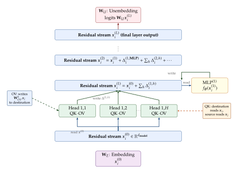
Head Composition across Layers
Single-layer attention heads implement simple operations. The true power of transformers emerges from composition: when the output of one head enters the residual stream and is read by a later head.
Q-Composition, K-Composition, and V-Composition
Let head be in layer and head be in layer . Head reads from the residual stream , which contains the contribution (averaged over the head attention pattern). Depending on which weight matrix of head is most sensitive to this contribution, we distinguish:
Q-Composition. Head 's output influences via . The virtual QK weight for the composed circuit is (Compose) which determines how head 's processing of destination token modulates what head attends to from source token .
K-Composition. Head 's output (at source position ) influences via . The virtual weight is (Compose) which controls how head 's processing of source token modulates what head attends to from .
V-Composition. Head 's output (at source position ) influences via . The virtual OV weight for the composed circuit is (Compose) which maps the original source residual stream (before head processed it) all the way to the output of head .
Definition 14 (Virtual Weights).
A virtual weight matrix is a product of two or more actual weight matrices, corresponding to a path through the transformer circuit graph that passes through the residual stream. Virtual weights reveal emergent relationships between tokens that cannot be detected by examining any single weight matrix in isolation. For a depth- transformer with heads per layer, the number of possible virtual weights grows as , and many of these correspond to identifiable functional circuits such as induction heads or copy suppression heads.
Induction Heads: A Canonical Example of Composition
The most studied example of two-layer head composition is the induction head circuit. Induction heads perform a simple but powerful operation: given a sequence containing , they predict to follow the second occurrence of by attending back to the first occurrence. This is achieved through the composition of two heads across layers:
A previous-token head in layer 1 (K-composition): attends from position to position , writing information about the previous token into the residual stream at each position.
An induction head in layer 2 (uses the layer-1 output via K-composition): attends from position to position where the previous-token residual stream at matches the current token at .
Together they implement the lookup: “find where my current token appeared before, and copy what came after it.” This is a two-layer circuit with measurable virtual weights, and its ablation causes a sharp drop in in-context learning performance.
Theorem: Decomposition of Transformer Output
We now state the fundamental decomposition theorem that makes transformer circuits mathematically tractable.
Theorem 3 (Linear Decomposition of Transformer Logits).
Let be a transformer with layers, attention heads per layer, weight-tied embeddings , and no layer normalisation (or with layer normalisation treated as an affine transformation absorbed into adjacent weights in the fold-LN approximation). For any target token and destination position , the logit decomposes exactly as (Decomp) where is the output of head in layer at position ((Update)) and is the output of the MLP block in layer . Each term is a scalar logit attribution that can be computed independently.
Proof sketch.
The proof is a direct consequence of the linearity of the residual stream and the linearity of the unembedding. By Definition 11, Applying the unembedding (a linear map) to both sides and taking the inner product with gives Since and we absorb the positional term into the direct path, the result follows. Each term depends only on the weights of the corresponding component (and the residual stream values it reads from, which depend on earlier components). This is an exact identity, not an approximation, given the stated assumptions.
Remark 10.
Real transformers apply layer normalisation before each sub-layer, which introduces a non-linearity that breaks the exact decomposition. The fold-LN approximation replaces each LayerNorm with its first-order linearisation around the mean activation, restoring additivity at the cost of a small approximation error. Empirically, this approximation introduces less than relative error in logit attributions for most positions, making it a practical tool.
Example: Information Flow in a 2-Layer Transformer
Example 3 (Tracing the Induction Circuit).
Consider a 2-layer, 2-head transformer processing the sequence (positions ) and predicting the next token after position 4.
Layer 1, Head 1 (previous-token head).
The QK circuit is learned such that position attends strongly to position . The OV circuit copies the source residual stream. Result: at each position , the residual stream is updated with information about token at position .
Concretely, at position 4 (A):
Layer 2, Head 1 (induction head).
The QK circuit of this head performs K-composition: it is sensitive to the
layer-1 residual stream at source positions, which now encodes the
previous token. The head at position 4 (token A) attends
strongly to position 2 (token B), because position 2's residual
stream contains a copy of position 1's token (A) from layer 1,
matching the current token.
The OV circuit then moves position 2's representation (B) to
position 4:
Logit attribution.
By Theorem 3, the logit for predicting B
next is dominated by
The induction head accounts for essentially all of the prediction boost
for token B. By ablating head , we can verify this
attribution experimentally: removing it causes the probability of
B to collapse to near-uniform.
Exercises
Exercise 13.
Let and .
Show that has rank at most .
Express the singular value decomposition of in terms of the SVDs of and , and show that the singular values of are products of those of and .
Given with smallest singular value , with largest singular value , and input norms , bound the maximum magnitude of the attention score before scaling by .
Exercise 14.
A copy head is an attention head whose OV circuit satisfies .
Show that a copy head with uniform attention over all source positions writes to the residual stream at every destination. What is the relationship between this operation and mean pooling?
If the QK circuit additionally implements a previous-token pattern (), describe the resulting circuit in natural language.
Suppose . Show that the head's update to the residual stream at destination is equivalent to adding a weighted sum of unembedding vectors, and explain how this could directly promote certain vocabulary items.
Exercise 15.
Consider a 3-layer transformer with a single head per layer, and suppose you have measured the OV circuits .
Write the virtual OV weight corresponding to a chain of V-compositions through all three layers: the output of head 1 is read by head 2's value circuit, and the output of head 2 is read by head 3's value circuit.
Show that this virtual weight is the product .
If has spectral norm at most for , bound the spectral norm of the virtual weight and comment on when deep composition amplifies or attenuates the original information.
Multi-Head Attention Decomposition
Having established the mathematical framework of transformer circuits in The Mathematical Framework of Transformer Circuits, we now turn to a systematic decomposition of multi-head attention as an information-routing mechanism. The central question is: given that the residual stream is a linear superposition of head contributions, can we interpret each head's contribution to the model's predictions? The answer is yes, through a combination of logit attribution, the logit lens technique, and a careful analysis of direct versus indirect effects through the residual stream.
Attention as Weighted Information Routing
The attention mechanism can be understood as a content-addressable memory lookup. At each destination position , the head broadcasts a query into the residual stream space and retrieves a weighted combination of values from source positions, where the weights are determined by query-key similarity.
More formally, using the circuit notation from The Mathematical Framework of Transformer Circuits, head in layer implements the routing: (Formal) where we have abbreviated for readability. The softmax over all source positions produces a probability distribution over source positions.
The routing metaphor.
Information at source position is routed to destination with weight . The OV circuit determines what information is moved: only the component of in the row space of can be moved at all. The QK circuit determines where to route: it scores every (destination, source) pair and produces a soft assignment.
Softmax Attention Patterns and Their Interpretation
Attention weights are produced by softmax, which has several interpretability implications.
Sparsity and entropy.
The entropy of the attention distribution, (Entropy) measures how diffuse the head's attention is. Low entropy (near ) indicates the head attends to a single source position-a hard lookup; high entropy (near ) indicates uniform attention over all positions-a soft average. Interpreting a head's function often begins with measuring this entropy: induction heads are sparse (they have found the right position to attend to), while positional heads may be diffuse (they average nearby positions).
Attention as a simplex-valued function.
The attention pattern (with , rows summing to 1) is a stochastic matrix. Its left eigenvectors decompose the pattern into interpretable modes: the dominant left singular vector of (the attention pattern with uniform background subtracted) often corresponds to a clear structural pattern such as attending to punctuation, the previous token, the subject of the sentence, and so forth.
Direct versus Indirect Effects through the Residual Stream
When we ask “what is the effect of head on the final logits?”, we must distinguish two types of contribution.
Definition 15 (Direct and Indirect Logit Attribution).
For head in layer , its direct logit attribution for token at position is (ATTR) the contribution of its output, unmediated, to the final logit. Its indirect logit attribution captures the effect of on later heads' attention patterns and MLP computations, propagated through the residual stream to the final logit. The total effect is (ATTR) where (indirect logit attribution) requires causal intervention (activation patching) to measure, since it involves the non-linear downstream processing of the head's output.
Remark 11.
Indirect logit attribution cannot be computed from the model weights alone; it requires activation patching experiments, where the head's output is replaced with its counterfactual value (e.g., from a different prompt) and the change in final logits is measured. For early layers, the indirect effect typically dominates; for the final layer, the direct effect is the only contribution. This is why logit lens (which only measures direct effects) is most interpretable for the final few layers.
The Logit Lens: Tracking Predictions Layer by Layer
The logit lens is a diagnostic technique introduced by Nostalgebraist that applies the unembedding matrix to intermediate residual stream states, revealing how the model's prediction evolves across layers. It exploits the decomposition from Theorem 3 to make the intermediate computation interpretable.
Definition 16 (Logit Lens).
For a transformer with layers, the logit lens at layer for target token and destination position is (LENS) the logit that would be assigned to token if the residual stream at layer were directly unembedded. The corresponding probability is .
The logit lens allows us to observe the model “changing its mind” across layers: an early layer might assign high probability to a syntactically plausible but semantically wrong continuation, which is corrected by later layers. This layer-by-layer evolution of predictions has been used to identify which layers perform which computational subtasks.
Relationship to the residual stream decomposition.
Note that (Decomp) the change in logit contributed by layer . This can be further decomposed head by head, giving a per-head, per-layer logit contribution chart.
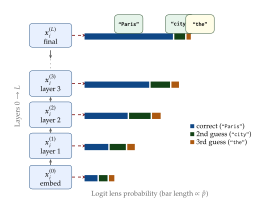
“Paris” has low probability; each subsequent layer
increases it monotonically (in this stylised example). The logit lens
makes the intermediate computations interpretable by projecting them
onto vocabulary space, showing which tokens the model is “considering”
at each depth.Proposition: Additivity of Head Contributions in Logit Space
We now prove the key structural result justifying per-head attribution.
Proposition 3 (Attention Head Contributions are Additive in Logit Space).
Under the fold-LN approximation, the logit for vocabulary item at position decomposes as an exact sum over individual head contributions and MLP contributions: (Logit) Each scalar term is the direct logit attribution of head to vocabulary item . The terms sum to the total logit without any cross-terms or interaction corrections.
Proof.
The proof follows directly from the linearity of both the residual stream and the unembedding operation. Recall that the final residual stream is (RS) The logit is a linear functional of (since is a linear map and the inner product with is linear). Applying this linear functional to both sides of (RS) gives This is (Logit) with the identification and . Since the residual stream decomposition is exact (under the fold-LN approximation), the logit decomposition is exact with no interaction terms.
Key Idea.
Each attention head implements a simple, interpretable operation; complexity emerges from composition. A single attention head is characterised by only two low-rank matrices: the QK circuit (which positions attend to which) and the OV circuit (what information is moved). Because these are rank- operators in a -dimensional space, each head has limited expressive power-it can only route a -dimensional slice of information. Yet from the composition of many such simple operations across many layers (with MLP blocks enabling non-linear feature construction between routing steps), transformers can implement extraordinarily complex functions. The appropriate unit of analysis is not the weight matrix but the circuit: the graph of information flow through the residual stream.
MLP Blocks: The Role of Feedforward Networks
While attention heads route information between positions, MLP blocks process each token's representation independently (they are applied position-wise with no cross-token communication). A standard two-layer MLP sub-block computes (DEF) where , , and is an element-wise activation (GELU or ReLU in practice).
The non-linearity is the key difference from attention heads: MLPs are not linear in the residual stream. However, the post-activation vector can be analysed neuron by neuron.
The “Attention Gathers, MLPs Compose” Hypothesis
Motivated by empirical findings in vision transformers and large language models, a key interpretability hypothesis has emerged:
Key Idea.
The “Attention Gathers, MLPs Compose” Hypothesis. Attention heads are the mechanism by which information is gathered across positions (routing relevant token representations to where they are needed), while MLP blocks are the mechanism by which gathered information is composed into higher-level features through non-linear computation. In video transformers and large language models, this division of labour is operationally separable: ablating attention heads destroys long-range context sensitivity, while ablating MLP blocks destroys feature construction and factual recall, but the two impairments are largely independent.
Empirical evidence for this hypothesis comes from several directions. In vision transformers (ViTs), attention heads in early layers perform local texture gathering, while MLP blocks in the same layers compute responses to features like edges and colour gradients. In large language models, factual knowledge is disproportionately stored in and recalled by MLP layers, while grammatical and positional relationships are implemented in attention layers.
Remark 12 (MLPs as Key-Value Memory Stores).
Geva et al. proposed viewing MLP blocks through the lens of key-value memory. Each neuron in defines a key pattern: the -th row of is a direction in residual stream space, and the neuron fires when the residual stream aligns with this direction. The corresponding column of defines the value written to the residual stream when the neuron fires. Under this interpretation, (Memory) which is a weighted sum of value vectors, where the weights are computed by matching the residual stream against key vectors. Experiments have shown that individual neurons in this decomposition correspond to specific facts: a neuron whose key fires on “the capital of France” and whose value promotes the token “Paris” in the unembedding space implements a single factual association. The MLP layer as a whole implements a soft retrieval over this distributed key-value store.
TikZ Figure: Attention versus MLP Division of Labour
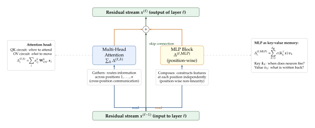
Exercises
Exercise 16.
Let and denote the probability distributions obtained by the logit lens at consecutive layers.
Show that the KL divergence depends on the norms and and the alignment of these vectors with the unembedding directions. (Hint: use the first-order approximation where .)
If layer has heads each contributing an OV update of norm and an MLP of norm (all in the same direction in residual stream space), what is the maximum possible logit change in terms of the unembedding norm ?
Describe qualitatively what “monotone logit lens” means (the correct token's probability increases monotonically across layers) and for which types of prompts you would expect to see this pattern versus a non-monotone pattern.
Exercise 17.
Consider a 2-layer transformer where layer 1 has one head, , and layer 2 has one head, .
Write the total logit for position as a sum of four terms: the direct path (embedding), head 's direct logit attribution, head 's direct logit attribution, and any cross-terms. Show that there are no cross-terms in the logit attribution, but that head 's output depends on head 's output through the residual stream.
Suppose you ablate head (set ) and observe that the logit decreases by . Decompose into head 's direct logit attribution and head 's indirect logit attribution (mediated through head ). Which term requires a second forward pass to compute?
If head is a V-composition predecessor of head (i.e., feeds into via the residual stream), show that the indirect effect of ablating head on head 's output is summed over .
Exercise 18.
This exercise explores the key-value memory interpretation of MLP blocks.
For an MLP with neurons and a ReLU activation, show that the output can be written as a sum over at most value vectors, where each value vector is gated by a non-negative scalar. What does this imply about the cone structure of MLP outputs?
Suppose neuron has key and value . Compute the contribution of this neuron to the logit for “Paris” when the residual stream contains a scaled copy of the “France” embedding, and show that it increases the probability of predicting “Paris”.
A superposition hypothesis states that neurons can represent near-orthogonal features (keys) in a -dimensional space via approximate orthogonality. If key vectors are drawn uniformly from the unit sphere in with and , compute the expected maximum inner product between any two keys and comment on the feasibility of this superposition.
Induction Heads and In-Context Learning
Among the most consequential discoveries of the mechanistic interpretability programme is the identification of a concrete, reusable computational motif called the induction head. Found independently in nearly every sufficiently large transformer trained on natural text, the induction head implements a form of pattern matching that appears to be the primary driver of in-context learning-the remarkable ability of large language models to adapt their behaviour from a few examples given in the input prompt, without any gradient update.
This section develops the mathematics of induction heads from the ground up. We begin with the simpler previous token heads that form in early layers of two-layer transformers, then show how a subsequent layer of attention heads exploits the key–value information produced by previous token heads to implement the completion pattern. We formalise the notion of K-composition by which two attention heads interact across layers, derive a mathematical characterisation of the attention pattern an induction head must implement, and place the discovery in its historical context as a major milestone on the path from black-box language modelling to circuit-level understanding.
Historical Note.
The transformer circuits thread. Mechanistic interpretability of transformers took a decisive turn in December 2021, when a team at Anthropic published a series of papers collectively called the Transformer Circuits Thread. The first instalment, “A Mathematical Framework for Transformer Circuits” (Elhage et al., 2021), introduced the residual-stream decomposition (sec:interp:residual-stream) and identified induction heads as a key primitive. The second major instalment, “In-context Learning and Induction Heads” (Olsson et al., 2022), showed that induction heads are not merely a curiosity of toy models but appear universally in transformers trained on text, and that their emergence during training coincides precisely with the sudden jump in in-context learning ability that practitioners had observed but not understood. This discovery marked the first time a concrete mechanistic explanation was offered for a macroscopic capability of a large language model, and it catalysed an explosion of work on circuit finding, superposition, and feature-level analysis.
Previous Token Heads
In a two-layer transformer, the first layer of attention heads performs computations on the residual stream before the second layer sees it. Empirically, several heads in layer 1 consistently learn a simple but strategically important operation: they attend almost exclusively to the token immediately preceding the query token in the sequence. We call these previous token heads.
Let the input sequence be , where each is a token index. The residual stream at position after the embedding and positional encoding is (Residual INIT) where is the token embedding and is the positional embedding. A previous token head with weight matrices computes attention scores (PREV ATTN Score) with a causal mask preventing attention to future positions. The empirical observation is that the learned weight product is dominated by a component that computes similarity between the positional embedding of position and the positional embedding of position . More precisely, if is a sinusoidal or learned positional embedding, then the product is large relative to any other pair, producing an approximately one-hot attention pattern .
The output of the previous token head at position is then (PREV Token Output) where is the output projection. This is added to the residual stream, so after layer 1 position contains information about both and : (Residual After L1) where denotes the linear map . This “token successor-context” representation in the residual stream is the key information that induction heads will exploit in layer 2.
Remark 13.
Previous token heads are not trained to be previous token heads by any explicit supervision signal. They emerge spontaneously during training because the previous-token pattern is a universally useful statistical regularisation: knowing what token preceded the current one is almost always helpful for prediction, and the sinusoidal positional encoding makes neighbouring positions geometrically similar in the key–query inner product space.
Induction Heads: the [A][B]...[A] [B] Pattern
An induction head is an attention head in layer 2 that implements a specific lookup procedure: when the current query position holds token (which has appeared before in the sequence), the induction head attends back to the position after the previous occurrence of token and copies the token that followed it.
Definition 17 (Induction Head).
Let be an attention head in layer of a transformer. is called an induction head if, for any sequence containing a repeated token at positions (so ), the attention pattern of satisfies (Induction ATTN) i.e., position attends primarily to position (the token immediately following the previous occurrence of ). The resulting output causes the residual stream at position to predict (the token that followed previously).
The key question is: how does position know to attend to position rather than ? The answer lies in K-composition with the previous token head (Previous Token Heads).
K-Composition Between Layers
Recall from sec:interp:residual-stream that the residual stream is a sum of contributions from all previous layers. The attention pattern of an induction head in layer 2 is determined by the inner product of query and key vectors, both of which are computed from the layer 2 residual stream . Because contains the output of previous token heads, the induction head's key at position encodes information about (the token before ). Meanwhile, the query at position encodes information about .
More precisely, the attention score of the induction head between query position and key position is (Induction Score) The layer-2 residual stream decomposes as , where is the previous token head output. If the induction head's key weight matrix is primarily sensitive to the “previous token” component , then (K COMP Expand) This is the virtual key contributed to position by the token . The effective key–query inner product (K COMP Inner) is large when is the same token as (i.e., when , the previous occurrence of ), so .
This is K-composition: the key of the layer-2 head is effectively composed with the value–output mapping of the layer-1 head, allowing the second layer to look up “which position follows the previous occurrence of the current token.”
Proposition 4 (Induction Head Attention Pattern).
Let be the OV-circuit of the previous token head, and let be the QK-circuit of the induction head. Define the composition matrix (COMP Matrix) If for some (i.e., the composition matrix is approximately a scaled identity), then the induction head attends to position with logit (Induction Logit) whereas all positions with receive logit approximately zero. Consequently, the softmax-normalised attention weight satisfies (Induction Softmax)
Sketch.
The logit at position under the dominant K-composition term is . If , this equals , which is when (i.e., ) and otherwise. For one-hot or nearly orthogonal embeddings, off-diagonal terms are near zero. Applying softmax yields the stated result.
Traced Example: A Concrete Induction Head Run
To build intuition, we trace the induction head on the classic nursery-rhyme continuation. Suppose the input sequence (tokenised) is:
The cat sat on the mat . The cat sat on the
The, cat, sat,
on, the, mat,
.. The subsequence repeats: positions – mirror
positions – (incomplete repetition; the model must predict
the continuation at position ).
At position (query token the, second occurrence), the
induction head proceeds as follows:
Query: The query vector at position encodes token
the(the same token type as position ).Key scan: The keys at positions – contain, in their “previous token” component, information about tokens respectively (using a dummy token at position ). Position has previous token
the(position , token ), so the K-composed key at position encodes tokenthe.Attention spike: Because the query encodes
theand the K-composed key at position also encodesthe, the attention logit is large. The softmax concentrates attention weight on position .Value read-out: Position holds token
mat(the token that followed the previous occurrence oftheat position ). The value–output circuit copies the representation ofmatinto the residual stream at position .Prediction: The model therefore strongly predicts
matas the next token-which is correct.
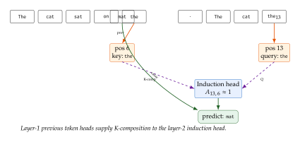
The cat sat on the mat. The cat sat on the$_12$”.
Orange boxes: previous token head representations in layer 1.
Blue box: induction head in layer 2 concentrating attention on
position 6 (the token after the previous the) via
K-composition. Green: value read-out predicting mat.
Why Induction Heads Work on Random Tokens
A striking experimental finding from Olsson et al. (2022) is that
induction heads operate equally well on random token
sequences-sequences drawn uniformly at random with no semantic
structure whatsoever. If the sequence is 7, 42, 13, 7,
the induction head at the second 7 correctly predicts
42 (the token that followed the first 7).
This is not a trivial observation. It rules out the hypothesis that induction heads work by learning semantic associations (“the word cat often follows the word the”). Instead, the mechanism is purely structural: it implements a sequence-level pattern-matching algorithm that can be described entirely in terms of token identities and relative positions.
Key Idea.
Pattern Matching, Not Semantics. An induction head implements the algorithm: “Find the most recent prior occurrence of the current token; output whatever followed it.” This algorithm is correct regardless of whether the tokens carry semantic meaning, making induction heads a form of in-context memorisation and replay rather than semantic generalisation. The implication for in-context learning is profound: a large language model can achieve few-shot performance not because it has learned a semantic rule from the examples, but because induction heads copy the pattern from the context window.
The random-token experiment also provides a quantitative diagnostic for induction head behaviour. Given a sequence of length of the form with drawn i.i.d. from a uniform distribution over the vocabulary, an ideal induction head achieves cross-entropy loss (Ideal LOSS) for the first repetition () and exactly zero loss for positions (since the pattern is perfectly predictable from context). In practice, models with strong induction heads achieve losses close to zero on the second half of such sequences, a metric called the induction-head loss used as a circuit-level benchmark.
The Phase Change: Sudden Emergence of In-Context Learning
Perhaps the most dramatic finding of the Olsson et al. (2022) study is the tight correspondence between the formation of induction heads during training and a sudden, non-linear improvement in in-context learning ability. The training curve of a large transformer on natural language exhibits a characteristic phase change:
Early training (before phase change): The model learns basic unigram and bigram statistics; the loss decreases smoothly. In-context learning ability (measured, for example, by how much the model benefits from in-context examples) is approximately zero. On random-token sequences, the second-half loss is approximately equal to the first-half loss.
The phase change: At a specific training step (which occurs earlier for larger models), the in-context loss drops sharply-over perhaps a factor-of-ten shorter window than the overall loss decrease. The model's ability to use in-context examples jumps discontinuously.
After the phase change: Induction heads are firmly established. The second-half loss on random-token sequences approaches zero. In-context learning ability is mature and roughly invariant to further training.
The mechanistic explanation is as follows. Induction heads form via a two-stage process:
In stage (a), previous token heads form in layer 1. This is a relatively gradual process.
In stage (b), having discovered the “previous token” information available in the residual stream, layer-2 heads rapidly reorganise to exploit K-composition. This is the sudden stage that produces the observed phase change.
The suddenness arises because K-composition is a multiplicative interaction: the gain from the induction-head algorithm scales as (the square of the K-composition strength), so once the previous token head is sufficiently strong, the gradient advantage of the induction-head algorithm becomes self-reinforcing.
Remark 14.
The phase change in in-context learning is a macroscopic, empirically observable phenomenon in large language models, not merely an artefact of toy-model analysis. Olsson et al. (2022) documented it in models with up to billions of parameters, and showed that the transition is faster (in training steps) for larger models. This is consistent with the “emergent abilities” discourse in the LLM scaling literature, but with a concrete mechanistic account: the emergence is not mysterious, but driven by the formation of a specific computational motif.
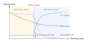
Exercises
Exercise 19.
Let the positional embedding be the sinusoidal encoding , .
Show that for all in the case (single frequency), i.e. the inner product between adjacent positional vectors is maximised.
Explain qualitatively why this property is not sufficient on its own to produce a previous token head: what additional learning must occur for the head to exclusively attend to the previous position?
In a relative positional encoding scheme (e.g., RoPE), the attention score depends on the relative position rather than absolute positions. How does this change the analysis? Would you expect previous token heads to form more or less readily?
Exercise 20.
The composition matrix from Proposition 4 measures the strength of K-composition.
Define the Frobenius composition score . Show that and that iff and have rank 1 and are aligned.
Elhage et al. (2021) proposed comparing for all pairs of heads as a heuristic for identifying composition in trained transformers. What are the limitations of this heuristic? (Hint: consider the case where both matrices are large but their product is small.)
Propose an alternative composition metric based on the spectral norm and discuss its computational cost compared to the Frobenius version.
Exercise 21.
Olsson et al. (2022) observed that the training step at which the phase change occurs scales approximately as for model size with .
Suppose that induction heads form when the K-composition strength exceeds a threshold . If the gradient of the loss with respect to scales as for some , derive a rough scaling law for in terms of , , and .
In your model, what is the implied relationship between and ? Is this consistent with the empirical finding that larger models form induction heads earlier?
Discuss at least one important confounding factor that your simple gradient-flow model ignores (e.g., interaction with the MLP layers, learning rate schedules, or weight regularisation).
The IOI Circuit - Interpretability in the Wild
The study of induction heads established that mechanistic interpretability can uncover real computational structure in trained transformers. But induction heads are, in some sense, a simple case: they form in two-layer models, they implement a single well-defined algorithm, and their function can be characterised by a handful of matrix products. The natural next question is whether the circuit-finding programme can scale to more complex, naturalistic tasks in full-sized models.
The answer was provided by Wang et al. (2022) in a landmark paper on the Indirect Object Identification (IOI) task in GPT-2 Small. The IOI task requires determining the indirect object of a sentence such as:
“John and Mary went to the store. John gave a drink to”
Key Idea.
A Neural Network Implements an Algorithm. The IOI circuit demonstrates that a transformer trained on next-token prediction has implicitly learned to implement a multi-step symbolic algorithm: (1) identify repeated names in the context; (2) determine which name is the subject (and therefore should be suppressed); (3) copy the remaining name to the output. This algorithm emerges not from any explicit symbolic supervision but from the structure of the pretraining data alone. Mechanistic interpretability's claim is that every sufficiently capable language model implements some algorithm in this sense, and that finding these algorithms is both scientifically valuable and practically important for AI safety.
The IOI Task: Formal Description
Definition 18 (IOI Template).
An IOI sentence is a sentence of the form
where is the subject name (a proper noun that appears twice) and is the indirect object name (a proper noun that appears once, after the conjunction and in the first clause). The target output is the token corresponding to . For example:[S] and [IO] [verb-phrase]. [S] [action-verb] a [object] to
John, Mary: “John and Mary went to the store. John gave a drink to Mary.”
Alice, Bob: “Alice and Bob visited the park. Alice handed a note to Bob.”
The task is defined by a dataset of such sentences; performance is measured by the logit difference (Logit DIFF) where and are the model's output logits for the indirect object and subject names respectively. A correct model satisfies .
GPT-2 Small (12 layers, 12 heads per layer, 768-dimensional residual stream) achieves on the IOI dataset (Appendix A of Wang et al., 2022), indicating that it reliably performs the task.
Head Roles in the IOI Circuit
The 26 attention heads in the IOI circuit play distinct functional roles, determined by their effect on the logit difference . Wang et al. identified four main categories:
Name Mover Heads
Name Mover Heads (NMH) are the final functional component of the IOI circuit: they read the indirect object name from its position in the context and copy it to the final token position (the position at which the model must predict the next token). The three most important NMHs are located in layers 9 and 10 of GPT-2 Small (heads 9.9, 9.6, and 10.0 in layer.head notation).
Mechanistically, NMHs implement a form of V-composition with earlier heads: their value–output circuit copies the name token embedding from the indirect object's position to the output residual stream. The OV matrix of a NMH satisfies , where projects the residual stream component corresponding to name tokens onto the logit space.
More precisely, if the residual stream at the position contains the representation and the NMH attends to that position with weight , the contribution to the final-position logits is (NMH Contribution) where is the unembedding matrix. When is approximately a scaled copy operator on name-token logits, this directly boosts relative to all other tokens.
S-Inhibition Heads
S-Inhibition Heads (SIH) serve the complementary role of suppressing the subject name at the final token position. Without SIHs, the model would predict both and with high probability (since both are plausible sentence completions in isolation), leading to errors on sentences where appears more recently in context.
The SIHs (principally heads 8.6, 8.10, and 7.3) sit in layers 7–8, above the duplicate token heads that detect the subject's repeated occurrence. Their query vectors at the final position attend to earlier positions that contain subject-name tokens; their value circuit then suppresses the corresponding name logit by writing a negative contribution to the residual stream at the final position: (SIH Contribution) where denotes the second (most recent) occurrence of the subject name, is a positive scalar, and is a unit vector selecting the logit. This suppression mechanism is what allows the model to distinguish the correct indirect object from the subject.
Duplicate Token Heads
Duplicate Token Heads (DTH) detect the fact that a name appears twice in the sentence-a key signal that identifies it as the subject. The DTHs (heads 0.1, 3.0, and others in early layers) attend from the second occurrence of a name token back to the first occurrence of the same name. Their OV circuit writes a “duplicated” signal into the residual stream of the second occurrence.
Formally, the key–query interaction of a DTH satisfies , where is a projection onto the subspace encoding proper-noun identity. As a result, position (second occurrence of subject ) attends strongly to position (first occurrence), and not to the single occurrence of .
Previous Token Heads in the IOI Circuit
The IOI circuit also contains previous token heads analogous to those discussed in Previous Token Heads. Here they serve the specific purpose of propagating name information from the name-token position to the token following the name (e.g., from “John” to “and” or from “Mary” to the verb phrase that follows). This enables later heads to attend to the name indirectly via its successor token, which is important for the sentence structures encountered in IOI templates.
Formal Definition of a Circuit
Definition 19 (Computational Circuit).
Let be the full computational graph of a transformer, where each node represents a computational unit (an attention head, an MLP sublayer, or a residual stream position), and each directed edge represents a data dependency (the output of node flows into node via the residual stream).
A circuit for a task is a subgraph with , such that:
Causal sufficiency: When all nodes in are replaced by their mean activations (i.e., ablated), the performance of the resulting model on is not significantly degraded compared to the full model.
Causal necessity: Each node is individually necessary: ablating (while keeping all other nodes) causes a significant degradation in performance on .
Minimality: No strict subgraph of satisfies both (a) and (b).
Remark 15.
The notion of “significant degradation” in Definition 19 is task-specific and must be given a quantitative threshold. For the IOI task, Wang et al. (2022) used a threshold of 50% reduction in the logit difference as the criterion for significance. The choice of threshold affects which heads are included in the circuit and is a source of sensitivity in the analysis.
Activation Patching: Verifying Causal Necessity
Demonstrating that a circuit is causally necessary-not merely correlated with the desired behaviour-requires an intervention methodology. The standard technique in the IOI paper (and the broader mechanistic interpretability literature) is activation patching (also called causal tracing or interchange intervention).
Definition 20 (Activation Patching).
Let be a clean input on which the model performs the task correctly, and let be a corrupted input (e.g., the same sentence but with the names swapped: ) on which the model does not. For a node with activation on the clean input and on the corrupted input, define the patched model as the forward pass of the corrupted input where is replaced by .
The causal effect of node is (Causal Effect) where is the logit difference ((Logit DIFF)). A large positive indicates that node carries causally relevant information for the task.
The activation patching procedure partitions the causal effect of a node into the portion attributable to the information it processes (rather than its architectural position), making it more interpretable than simple ablation.
In the IOI analysis, activation patching was applied systematically to every attention head in every layer of GPT-2 Small, producing a heat-map of causal effects across the 1212 = 144 heads. The heads with the largest effects are precisely the NMHs, SIHs, DTHs, and previous token heads identified in the circuit-providing strong evidence that these heads are causally, not merely correlationally, important.
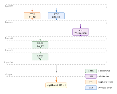
Step-by-Step Circuit Walkthrough
We now trace the IOI circuit on the sentence:
“John and Mary went to the store. John gave a drink to”
Step 1: Duplicate Token Heads detect the repeated name.
At position 9 (the second John), the DTHs attend strongly to position 1 (the first John), because both positions share the same name embedding. This writes a “duplicate” signal into the residual stream at position 9, flagging it as the second occurrence of a name.
Step 2: Previous Token Heads propagate context.
At positions 2 and 10 (the tokens immediately following each John), the previous token heads write information about John into the residual stream. Similarly, at position 4 (following Mary), the previous token head writes information about Mary. This propagation ensures that later heads have access to name identity from both the token itself and its successor.
Step 3: S-Inhibition Heads suppress the subject.
At the final query position (the token “to,” which precedes the predicted token), the SIHs in layers 7–8 scan backwards. Their attention weights are concentrated on position 9 (the second, most recent, occurrence of John), particularly because position 9 carries the “duplicate” signal from Step 1. The SIHs' OV circuit writes a negative signal to the residual stream that reduces the logit of the token John.
Step 4: Name Mover Heads copy the indirect object.
At the final position, the NMHs in layers 9–10 attend to position 3 (Mary). Their attention is guided by the absence of a duplicate signal at position 3: Mary appears only once, so the NMHs' QK circuit selects it over the (now-suppressed) John. The OV circuit of the NMHs copies the Mary embedding into the final residual stream.
Step 5: Unembedding.
The final residual stream, boosted toward Mary by the NMHs and away from John by the SIHs, is projected through the unembedding matrix . The result is , i.e., the model correctly predicts Mary as the continuation.
Example 4.
On the sentence “Alice and Bob visited the park. Alice handed a note to”, GPT-2 Small produces (approximately): Ablating the three NMHs (replacing their outputs with their mean activations) reduces to approximately -a reduction of 60%, confirming that NMHs are causally important. Ablating the three SIHs reduces to approximately (a 53% reduction), confirming the importance of suppression. Ablating both simultaneously reduces below zero, causing the model to incorrectly predict Alice.
Warnings and Limitations
Caution.
Circuits found in toy or constrained models may not generalise. The IOI circuit was identified in GPT-2 Small (117M parameters) under a specific set of template sentences. Several caveats apply:
Template sensitivity: The IOI dataset uses stylised sentences with a fixed grammatical template. The circuit's structure may change for more varied sentence forms (e.g., sentences with more than two names, or indirect objects expressed via pronouns).
Model size: Larger models may implement the same function with different circuits-or distribute the computation across more heads, making the circuit larger and harder to isolate. There is no guarantee that GPT-2 Small's IOI circuit appears in GPT-4 or Claude.
Polysemanticity: The same attention head may contribute to multiple circuits simultaneously (The Superposition Hypothesis). Ablating a head to test necessity in one circuit may inadvertently affect its role in other circuits, contaminating the causal analysis.
Mean ablation as a baseline: Replacing a node's activation with its mean over the dataset is a methodological choice; other ablation baselines (zero ablation, noise injection, random activation from the dataset) give different results.
Faith\-fulness vs. completeness: Wang et al. (2022) demonstrated that the IOI circuit is faithful (its behaviour on IOI sentences matches the full model's) but did not claim it is the unique circuit implementing the task. Other subgraphs might implement the same function.
Despite these caveats, the IOI circuit remains the most thoroughly validated mechanistic account of a realistic NLP behaviour, and its methodology has become the template for subsequent circuit analyses.
Broader Implications for Interpretability Research
The IOI circuit contributes several lasting methodological lessons to the interpretability programme:
Functional decomposition is possible at scale.
Despite GPT-2 Small's 144 attention heads and 12 MLP sublayers, a mere 26 heads are causally sufficient for the IOI task. This suggests that transformers do not distribute all computations diffusely across all components, but concentrate specific functions in identifiable subsets.
Algorithm identification bridges symbolic and neural views.
The four-step algorithm identified in Step-by-Step Circuit Walkthrough (detect duplicate, propagate context, suppress subject, copy object) is a symbolic description of a computation performed by continuous, high-dimensional neural network activations. This bridging of levels is precisely what mechanistic interpretability aspires to achieve for all model behaviours.
Causal methodology is essential.
The combination of activation patching, attention visualisation, and ablation provides converging evidence that is more compelling than any single method alone. Correlation-based analyses (attention visualisation without patching) would have identified the same heads as “interesting,” but could not establish causal necessity. The IOI paper's causal methodology is now standard in circuit-finding work.
Safety relevance.
The IOI task is innocuous, but the methodology it validated is directly applicable to safety-relevant behaviours: deception, refusal, sycophancy, hallucination. If a model's tendency to produce false confident statements is implemented by a specific circuit, that circuit can potentially be identified, patched, or monitored. This is one of the primary motivations for the broader mechanistic interpretability programme.
Insight.
The IOI circuit demonstrates that the question “what algorithm does this model implement?” is not merely philosophical but empirically tractable. The difficulty scales with the complexity of the behaviour; finding the “truthfulness circuit” or the “deception circuit” in a frontier model is vastly harder than the IOI case. But the IOI result establishes that the question is answerable in principle, and provides the methodological toolkit to pursue it.
Exercises
Exercise 22.
Consider a simplified version of the IOI task in which only a single Name Mover Head (NMH) and a single S-Inhibition Head (SIH) are active, and their contributions to the final logit difference are additive: , where and .
Under mean ablation of the NMH (i.e., setting ), the logit difference drops to . Under mean ablation of the SIH (setting ), it drops to . If the total logit difference is and ablating the NMH gives , estimate and .
Suppose the NMH and SIH interact: the SIH's contribution depends on how strongly the NMH fires. Propose a modified model and derive the individual causal effects under mean ablation. What sign would you expect to have, and why?
When does the additive model systematically overestimate the causal importance of the NMH? Provide a concrete example using the interactive model from (b).
Exercise 23.
The minimality condition in Definition 19 requires that every node in the circuit is individually necessary.
Show that the following graph is not minimal as a circuit for a binary task: nodes and both contribute to the output logit, the threshold for success is , and each node individually reaches the threshold. Propose the minimal circuit.
In practice, “individually necessary” is tested by a threshold on performance degradation (e.g., reduction in ). Construct a counterexample in which two heads are each individually below the threshold (e.g., ablating either causes only 30% degradation) but together they are necessary (ablating both causes 80% degradation). What does this suggest about the adequacy of the standard minimality test?
Propose a revised definition of minimality that handles the counterexample from (b). Your definition should be computationally tractable (not requiring exponential enumeration of all subsets).
Exercise 24.
Wang et al. (2022) studied GPT-2 Small. This exercise asks you to think about how their findings might or might not generalise.
Suppose we train a transformer with twice the number of attention heads per layer (24 instead of 12) on the same data. Give two distinct hypotheses for how the IOI circuit might change: (H1) the same circuit is distributed over more heads (“redundancy hypothesis”); (H2) a qualitatively different circuit implements the same function more efficiently. For each hypothesis, describe an experiment that would distinguish it from the other.
The IOI task uses proper names (e.g., John, Mary). Propose an analogous task that uses common nouns instead (e.g., cat, dog) and describe which components of the IOI circuit you would expect to generalise directly and which you would expect to differ. Justify your prediction based on the mechanistic descriptions in Head Roles in the IOI Circuit.
A critic argues that the IOI circuit is an artefact of the specific IOI dataset used and that GPT-2 Small's IOI performance is driven by memorisation of training sentences rather than a generalisable algorithm. Design an experiment to test this hypothesis rigorously. What would you measure, and what outcome would confirm or refute the critic?
The Superposition Hypothesis
One of the most striking findings in mechanistic interpretability is also one of the most counterintuitive: individual neurons are not individual concepts. Open a dictionary and each entry denotes exactly one word. Look up a neuron in a transformer and you will find it responds to dozens of unrelated stimuli - currency symbols, geographical locations, names of chemical elements, expressions of negation. This is not a flaw in how we measure neurons; it reflects something deep about how neural networks choose to organise information internally.
The superposition hypothesis, developed at Anthropic in a landmark series of papers on toy models of superposition, proposes a precise explanation: neural networks store more features than they have neurons by packing those features into nearly orthogonal directions in activation space. The inevitable price is interference - features “bleed” into one another whenever two features that share a neuron happen to be active simultaneously - but if features are sparse (rarely co-active), the expected interference is small and the gain in representational capacity is large.
This section develops the mathematics of superposition rigorously. We begin with the formal definition (Formal Definition of Superposition), then study a toy model that makes the phenomenon concrete and analytically tractable (The Toy Model of Superposition). We connect the geometry to the celebrated Johnson–Lindenstrauss lemma (The Johnson–Lindenstrauss Lemma and Superposition Capacity), derive the phase diagram governing when a network chooses to superpose a feature (Phase Transitions in Superposition), and close with a striking biological analogy: sparse coding in the mammalian visual cortex (Biological Connection: Sparse Coding in Visual Cortex).
Historical Note.
From grandmother cells to distributed codes. The debate between localist and distributed representations in neural systems has raged for decades. Localist theories, epitomised by the apocryphal “grandmother cell” hypothesis of Konorski (1967), hold that single neurons encode single concepts. Barlow's “feature detector” neuroscience (1972) provided partial support: certain retinal ganglion cells clearly signal oriented edges. But Hinton, McClelland, and Rumelhart (1986) argued forcefully for distributed representations in their parallel distributed processing volumes. In machine learning, the linear representation hypothesis - that neural networks encode features as directions in activation space - emerged from early work on word embeddings (Mikolov et al., 2013) and was formalised by the concept of residual stream in transformer mechanistic interpretability (Elhage et al., 2021). The superposition hypothesis is the natural culmination: if features are directions, and if there are more concepts to represent than dimensions available, superposition is not merely possible but necessary.
Why Neurons Are Polysemantic
Consider a language model processing a sentence about Paris. The model must track, among other things, the grammatical role of “Paris”, its semantic category (proper noun, city, capital), its cultural associations (Eiffel Tower, haute cuisine, fashion week), and its position in the discourse. In a network with neurons in a hidden layer, the model must represent all of these features - and thousands more - using vectors in .
The naive solution is monosemanticity: assign one neuron to each feature. This is clean, interpretable, and utterly impractical. Modern language models process tokens drawn from vocabularies of tens of thousands, appearing in contexts that invoke hundreds of thousands of distinct semantic properties. No realistic hidden dimension can accommodate a dedicated neuron per feature.
Key Idea.
Neural networks represent more concepts than they have neurons - this is both powerful and problematic. Powerful because it grants exponential representational capacity in the number of features for the cost of a linear number of neurons; problematic because it makes individual neurons uninterpretable and renders activation patching unreliable.
The fundamental tension is between two desiderata. First, the network wants representational capacity: the ability to track many features simultaneously. Second, it wants interpretability: a clean mapping between neurons and concepts. Superposition is the network's resolution to this tension, sacrificing interpretability for capacity.
To see why this trade-off arises naturally from gradient descent, recall that a neural network's loss function cares only about predictions, not about the interpretability of intermediate representations. If packing two features into one neuron reduces loss (because both features are useful but rarely co-active), gradient descent will discover this packing automatically. There is no mechanism imposing monosemanticity.
Formal Definition of Superposition
We formalise the notion of superposition in terms of the linear representation hypothesis.
Definition 21 (Feature and Feature Direction).
A feature is a binary or real-valued property of an input that is causally relevant to the model's output. Under the linear representation hypothesis, each feature is represented as a direction in the activation space of a layer with hidden dimension , such that the activation vector can be written as (Linear REPR) where is the number of features, is the feature activation, and is noise.
Definition 22 (Superposition).
A layer with hidden dimension is said to exhibit superposition when the number of represented features exceeds the layer dimension (i.e., ), and the feature directions form a set of nearly orthogonal unit vectors satisfying (Superp EPS ORTH) for some small . The feature directions form a superposition dictionary.
Remark 16 (Near-orthogonality vs. exact orthogonality).
Exact orthogonality of vectors in is impossible by elementary linear algebra: any set of more than vectors in must be linearly dependent. The key insight of the superposition hypothesis is that near-orthogonality is achievable for , and near-orthogonality is sufficient for low interference when features are sparse.
The Toy Model of Superposition
To make the superposition hypothesis analytically tractable, Elhage et al. (2022) introduced an elegant toy model: a one-hidden-layer autoencoder that attempts to reconstruct features using only dimensions.
Model architecture.
Let be a sparse feature vector, where each component is nonzero with probability (the feature's “sparsity”) and, when active, takes value drawn from some distribution (for simplicity, with ). The model maps through a linear bottleneck: (TOY Encode) where is the weight matrix (the superposition dictionary), and the ReLU nonlinearity enforces non-negativity of the reconstructed features. The training objective is a weighted mean-squared error: (TOY LOSS) where is the importance of feature (proportional to how much the model cares about reconstructing it accurately).
What does the model learn?
Two extreme solutions exist. In the monosemantic solution, the model sets (impossible here since ) or selects the most important features and represents each in a dedicated dimension, ignoring the rest. In the superposition solution, the model represents all features using nearly-orthogonal directions in , accepting small reconstruction errors whenever two features are simultaneously active.
The expected reconstruction error for feature under superposition is: (TOY Interference) where the right-hand side accumulates squared inner products weighted by the co-activation probability . When features are sparse ( for all ), this error is small even if the are only approximately orthogonal.
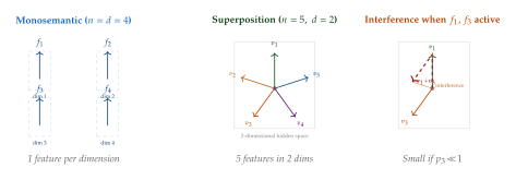
Optimal geometry.
A natural question is: what arrangement of unit vectors in minimises the total squared interference ? This is the Tammes problem (also called the Grassmannian packing problem). For , the optimal solution is the regular simplex: vertices of the regular -simplex inscribed in the unit sphere . For larger , the optimal packings are known for special cases (e.g., gives the cross-polytope) but are generally NP-hard to compute.
The toy model trained by gradient descent nonetheless discovers near-optimal solutions, suggesting that the loss landscape has favourable geometry for superposition.
The Johnson–Lindenstrauss Lemma and Superposition Capacity
How many features can a -dimensional space accommodate in superposition? The answer is surprisingly large, and its theoretical foundation is the celebrated Johnson–Lindenstrauss (JL) lemma.
Proposition 5 (Near-Orthogonal Vectors in ).
For any , there exists a set of (NEAR ORTH Bound) unit vectors in such that for all .
Proof sketch.
The argument follows from a probabilistic construction. Draw independent random unit vectors uniformly from the unit sphere . For any fixed pair with , the inner product is a sub-Gaussian random variable with mean zero and variance (by symmetry of the uniform distribution on ).
By the Hoeffding-type concentration inequality for the sphere: (JL Concentration) By a union bound over all pairs, the probability that any pair violates the -orthogonality condition is at most (JL Union) This probability is less than 1 (i.e., a valid -orthogonal set exists with positive probability) as long as , i.e., . Since the construction is existential, the bound follows.
Remark 17 (Exponential capacity).
Proposition 5 implies that a -dimensional hidden layer can in principle represent features in -superposition. The explicit union bound above carries the constant : for and it already guarantees more than near-orthogonal directions, vastly more than the strictly orthogonal directions that fit exactly. At the looser tolerance the same explicit bound gives only : the from this crude union bound is far from tight. The practically relevant regime is moderate (say –) and large , where the exponential capacity vastly exceeds .
The JL lemma (in its original form) states that any set of points in can be embedded into (with ) while preserving all pairwise distances to within a factor of . The connection to superposition is direct: if we regard features as points on the unit sphere, a random projection into dimensions (the “compression” step) preserves their near- orthogonality, exactly the geometric property that makes superposition work.
Theorem 4 (Johnson–Lindenstrauss Lemma).
Let and let be any -point set. Set . Then there exists a linear map such that for all : (JL Lemma) Moreover, a random Gaussian matrix satisfies this with probability at least .
The implication for neural networks is profound: the weight matrix of a linear layer can act as a random projection, preserving the approximate geometry of the feature space even when the bottleneck dimension . Superposition is, in a sense, the neural network's implicit implementation of the Johnson–Lindenstrauss construction.
Phase Transitions in Superposition
The toy model of The Toy Model of Superposition reveals a sharp phase transition: depending on the importance and sparsity of a feature, the model either represents it cleanly (monosemantically) or superimposes it with other features, or ignores it entirely.
Three phases.
Consider a model with (one-dimensional hidden space) and features with importances and sparsities . The model must choose how to allocate its single dimension. The optimal solution depends on the trade-off between:
Monosemantic: represent only feature 1, giving loss .
Superposition: represent both features as (antipodal), giving interference loss (the antipodal cross terms cost error only when both features co-activate, probability ).
Ignore both: loss .
Superposition is preferred when the interference loss is lower than the monosemantic loss: (Phase COND) This condition is satisfied precisely when feature 1 is sparse (), so that the interference it causes is rare enough that sharing the dimension still beats paying to ignore feature 2.
General phase diagram.
In the general setting with features, the phase diagram lives in the space of pairs. Three regimes emerge:
Clean representation (high importance, high density): the model allocates a dedicated dimension, achieving exact reconstruction.
Superposition (moderate importance, low density): the model packs multiple features into shared directions, accepting small interference.
Dropped feature (low importance): the model ignores the feature entirely, setting .
Remark 18 (Practical implications).
The phase diagram predicts that rare, important features are most likely to be in superposition: they are important enough to include but sparse enough that interference is manageable. This matches empirical findings: in practice, features corresponding to rare tokens, unusual syntactic constructions, or domain-specific terminology tend to be polysemantically encoded, while high-frequency features (e.g., the “is this a space character?” detector) often achieve near-monosemantic representations.
Biological Connection: Sparse Coding in Visual Cortex
The superposition hypothesis does not arise in a vacuum: it has a remarkable parallel in neuroscience. In 1996, Bruno Olshausen and David Field published a seminal paper showing that the receptive fields of simple cells in the primary visual cortex (V1) can be derived from a sparse coding principle applied to natural images.
The Olshausen–Field model.
Given a patch of a natural image, Olshausen and Field proposed learning a dictionary (with , an overcomplete dictionary) and a sparse code such that with sparse. The learning objective is: (Olshausen Field) where the second term encourages sparsity in the code. When trained on natural image patches, the columns of spontaneously develop into oriented, localised, bandpass filters - precisely the Gabor-like receptive fields observed in V1 neurons.
The connection to superposition.
The parallel is striking:
The dictionary plays the role of the superposition dictionary , with overcomplete columns () analogous to .
The sparse code plays the role of the feature activations , with sparsity enabling efficient representation.
The Gabor-like columns of correspond to monosemantic feature directions: each column encodes a single oriented edge at a specific spatial frequency.
The brain appears to have independently discovered the same solution to the representational bottleneck that gradient descent finds in artificial neural networks: pack more features than dimensions by exploiting sparsity.
Remark 19 (Differences from the neural network case).
There are important differences. The visual cortex operates in an approximately monosemantic regime at the level of V1 simple cells: each cell responds to a specific orientation, spatial frequency, and position. The superposition-like behaviour in artificial networks is more extreme: the same neuron may respond to linguistically unrelated concepts. One reason is that V1 has far more neurons than necessary to represent the relevant features of natural images (the cortex is massively over-resourced at this stage), while artificial models are typically under-resourced relative to the number of semantic features in language.
Exercises
Exercise 25.
Interference bound. Consider unit vectors arranged as the vertices of a regular -simplex inscribed in the unit sphere (assuming ). Show that for this configuration, for all . Then compute the total squared interference and show that it equals . Conclude that the simplex achieves the minimum total squared interference among all unit-norm configurations (you may cite the Welch bound without proof).
Exercise 26.
Sparsity and phase transitions. Extend the two-feature phase analysis of Phase Transitions in Superposition to three features with equal importances and equal sparsities , in a hidden space of dimension . Consider the three candidate solutions: (a) monosemantic: represent the two most-important features in orthogonal dimensions, drop the third; (b) superposition with a regular triangle: represent all three features as the vertices of an equilateral triangle inscribed in the unit circle; (c) superposition with a square: represent two features orthogonally and pack the third as . Compute the expected loss for each solution as a function of and determine which solution is optimal for .
Exercise 27.
JL capacity scaling. Let and consider the bound from Proposition 5. (a) Compute the maximum number of -nearly-orthogonal unit vectors in for using the exponential bound . (b) A transformer model with hidden dimension is claimed to represent semantic features in superposition. What is the implied average squared inner product if the features are arranged as uniformly random unit vectors? Is this consistent with low interference when feature sparsity is ? (c) How does the capacity scale if we allow instead of ? What practical trade-off does this represent?
Sparse Autoencoders for Feature Discovery
If the superposition hypothesis is correct, then the fundamental challenge of mechanistic interpretability is not merely to find what neurons do, but to disentangle the superimposed features from the directions in which they are packed. The neuron basis is the wrong basis; we need to find the feature basis.
This insight motivates a deceptively simple idea: train a sparse autoencoder (SAE) on the model's activations. The autoencoder is forced to reconstruct the activations using a small number of active dictionary elements at each forward pass. If the training is successful, those dictionary elements will correspond to the monosemantic features that the network has superimposed - the SAE effectively inverts the superposition and recovers the feature basis.
The field of SAE-based interpretability has exploded since Cunningham et al. (2023) and the Anthropic team (Templeton et al., 2024) demonstrated that SAEs trained on transformer activations discover human-interpretable monosemantic features at scale. This section develops the theoretical foundations, practical training considerations, and empirical findings of this methodology.
Historical Note.
From dictionary learning to mechanistic interpretability. Sparse autoencoders as a machine learning technique predate their use in interpretability by decades. The connection to sparse coding (Olshausen and Field, 1996) is direct: an SAE is essentially a learned overcomplete dictionary, trained by gradient descent rather than by pursuit algorithms. In signal processing, sparse representations and basis pursuit (Chen, Donoho, and Saunders, 1998) provided a rigorous foundation for recovering sparse signals from compressed measurements. The application to neural network interpretability was first proposed by Cunningham et al. (2023), who demonstrated that SAEs trained on one-layer transformers recover interpretable features. Templeton et al. (2024) scaled this to Claude 3 Sonnet, discovering over a million interpretable features including multimodal concepts spanning language, emotion, and abstract reasoning.
SAE Architecture
A sparse autoencoder is a two-layer neural network with an expansion factor: the hidden dimension is much larger than the input dimension (i.e., ). The key constraint is that the hidden representation must be sparse: only a small fraction of the hidden units are active for any given input.
Definition 23 (Sparse Autoencoder for Mechanistic Interpretability).
A sparse autoencoder (SAE) for mechanistic interpretability is a pair of functions where: (SAE Encoder) where is an activation vector from the target layer, is the encoder weight matrix, is the decoder weight matrix (with unit-norm columns: for all ), is a pre-encoder bias applied before encoding and re-added after decoding, is the encoder bias, and is the sparse feature activation vector.
Remark 20 (Role of the pre-encoder bias).
The pre-encoder bias centres the input distribution before encoding. Without it, the ReLU nonlinearity would impose an asymmetric constraint on the features: features would only be able to represent positive deviations from zero rather than deviations from the mean. Centering allows the encoder to detect both positive and negative excursions of each feature, with the ReLU then selecting only the positive excursions as active.
Dictionary elements.
The columns of , denoted for , are the dictionary elements of the SAE. Each dictionary element is a direction in activation space. When the SAE is trained successfully, each should correspond to a monosemantic feature: a single, human-interpretable concept.
The encoder computes a non-negative coefficient for each dictionary element, with indicating that feature is active in the current context. The decoded reconstruction expresses the activation as a sparse linear combination of dictionary elements.
Training Objective
The SAE training objective balances two competing goals: reconstruction fidelity (the decoded should match the original closely) and sparsity (only a few dictionary elements should be active at each step).
Definition 24 (SAE Training Objective).
The SAE training loss is: (SAE LOSS) where is the sparsity coefficient controlling the trade-off between reconstruction quality and sparsity of the hidden representation. The norm (with by construction) penalises the total magnitude of feature activations.
Remark 21 (Why and not ?).
The “norm” directly counts the number of active features and is the theoretically cleanest sparsity measure. However, is non-differentiable and NP-hard to optimise. The norm is the convex relaxation of : it is the tightest convex surrogate that still promotes sparsity. Under certain conditions (the restricted isometry property), minimisation exactly recovers the sparsest solution. In practice, the penalty combined with a ReLU encoder provides an effective and gradient-friendly sparsity constraint.
Normalisation of decoder columns.
A crucial subtlety: the decoder columns must be constrained to have unit norm. Without this constraint, the optimiser can trivially reduce the sparsity penalty by rescaling: make very large (absorbing the scale into ) and make very small (reducing ). Unit-norm columns prevent this degeneracy. In practice, this is enforced by projecting onto the Stiefel manifold after each gradient step: (SAE NORM)
Hyperparameter sensitivity.
The sparsity coefficient is a critical hyperparameter. Too small: the SAE learns a near-dense representation with high reconstruction fidelity but uninterpretable features (the trivial solution is to learn the identity mapping with ). Too large: the SAE learns to use very few features, sacrificing reconstruction fidelity to the point where many input dimensions are ignored. The optimal must be found by balancing reconstruction loss and sparsity, often using metrics like (average number of active features per token) and reconstruction .
The Shrinkage Problem
A fundamental limitation of -penalised estimation, long recognised in the statistics literature under the name LASSO shrinkage, is that it systematically underestimates the magnitude of large coefficients.
The bias of LASSO.
Suppose the true feature activation for feature in context is . Under the penalty, the optimal estimate is the soft-thresholding operator applied to the pre- activation : (SOFT Threshold) where is the soft-thresholding function with threshold . The bias is whenever (the feature is active). This means:
Active features have their magnitudes systematically underestimated by .
The SAE must compensate by adjusting the decoder columns , potentially distorting the feature geometry.
Features with true activation are entirely suppressed to zero, even if they are genuinely active.
Remark 22 (Practical impact of shrinkage).
Shrinkage biases the SAE's estimate of feature magnitudes. In mechanistic interpretability, we often care not just about which features are active but how strongly they are active (e.g., to determine causal influence on model output). Shrinkage makes it harder to reliably estimate feature strengths, potentially causing interpretability analyses to underestimate the importance of certain features.
Gated SAEs: Separating Gating from Magnitude
The shrinkage problem arises because a single value () must simultaneously encode two distinct decisions: (1) is feature active? (a binary gating decision) and (2) how strongly is feature active? (a continuous magnitude). The penalty acts on the magnitude, but its effect is felt through the gating decision as well.
Gated SAEs (Rajamanoharan et al., 2024) resolve this by introducing separate pathways for gating and magnitude estimation.
Definition 25 (Gated Sparse Autoencoder).
A Gated SAE replaces the standard encoder with a two-pathway architecture: (Gated GATE) where are separate gating and magnitude weight matrices, is the binary gate computed via the Heaviside step function with straight-through estimation (STE) for backpropagation, and denotes element-wise multiplication.
Loss modification.
The gated SAE uses a modified loss that places the sparsity penalty on the gate logits rather than the final activations: (Gated LOSS) The sparsity penalty acts on (the smooth version of the gate) rather than on the magnitude activations, decoupling the gating and magnitude estimation problems.
Empirical improvements.
Gated SAEs consistently outperform standard SAEs on the reconstruction–sparsity Pareto frontier: for the same level of sparsity (average ), gated SAEs achieve lower reconstruction error, and for the same reconstruction error, they achieve lower . The interpretability of discovered features is also qualitatively improved, suggesting that clean gating leads to cleaner feature separation.
Transcoders: Mapping MLP Input to Output
Standard SAEs are trained on residual stream states: the activations before or after a given layer. An alternative, proposed by Dunefsky et al. (2024), is the transcoder: a sparse model that maps the input to an MLP layer directly to its output.
Definition 26 (Transcoder).
A transcoder is a learned function that approximates a transformer MLP sublayer , parameterised as: (Transcoder ENC) where is the MLP input, approximates the MLP output, and is the sparse intermediate representation with . The training loss is: (Transcoder LOSS)
Advantages of transcoders.
The transcoder provides a fundamentally different perspective from residual-stream SAEs. Whereas a residual-stream SAE decomposes “what information is stored at a given position”, a transcoder decomposes “what computation the MLP performs”. Specifically, the dictionary elements of the transcoder are input-output pairs: active feature contributes to the output, where describes the direction in which that feature updates the residual stream.
This makes transcoders particularly suitable for understanding knowledge storage in MLP layers, where factual associations (e.g., “Paris is the capital of France”) are believed to be stored as superimposed key-value pairs (Meng et al., 2022 - ROME).
SAE Architecture: A Visual Overview
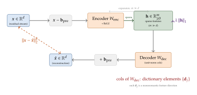
Monosemantic Features: What SAEs Discover
The proof of the SAE methodology lies in what it finds. When SAEs are trained on the internal activations of large language models, the dictionary elements exhibit striking monosemanticity: each element responds strongly to a specific, human-interpretable concept and weakly to everything else.
Categories of discovered features.
SAE features can be broadly grouped into three categories:
Geographic features. Features that activate strongly for tokens that are part of geographical references - country names, city names, continent names, or demonyms. Different features distinguish different granularities and types: one feature may activate for “European capital city names”, another for “South American river names”, a third for “US state abbreviations”.
Temporal features. Features encoding temporal information: specific decades (“1990s”, “2000s”), recurring events (“every year”, “annual”), temporal expressions (“yesterday”, “next month”), and calendar dates. Temporal features often have a strong interaction with domain: “1990s technology” and “1990s music” may activate different features despite sharing the decade marker.
Conceptual and relational features. Features for abstract semantic relationships: negation, causality, analogy, contrast, and entailment. Also present are syntactic features (subject-verb agreement, genitive markers), domain markers (medical terminology, legal jargon, code syntax), and emotion/sentiment features.
Insight.
SAEs are microscopes for neural networks - they reveal individual features the way microscopes reveal cells. Just as a light microscope cannot distinguish organelles (requiring electron microscopy), a SAE with a small dictionary ( comparable to ) cannot distinguish fine-grained features. But as the dictionary size grows (analogous to increasing magnification), progressively finer-grained features become visible.
Validation of monosemanticity.
How do we verify that a discovered feature is genuinely monosemantic? The standard approach is automatic interpretability (Bills et al., 2023): use a separate language model (e.g., GPT-4) to generate a natural-language description of the feature by examining the top-activating tokens and contexts, then evaluate whether the description correctly predicts which new contexts will activate the feature. A feature is considered monosemantic if a single short description achieves high prediction accuracy.
Templeton et al. (2024) applied this methodology at scale to Claude 3 Sonnet, finding that the majority of the 1,000,000+ discovered SAE features received high-quality monosemantic descriptions from the automated evaluator.
Scaling SAEs: Dictionary Size, Dead Features, and Fidelity
Training SAEs at scale introduces new challenges that do not appear in small-scale experiments. Three phenomena dominate the scaling behaviour of SAEs: the dictionary size, the dead feature problem, and the reconstruction fidelity trade-off.
Dictionary size and feature granularity.
As the dictionary size increases, the SAE discovers progressively more fine-grained features. With , an SAE trained on a language model might discover a single “European country” feature. With , it discovers separate features for each European country. With , it distinguishes not only countries but also contexts (“France as a tourist destination”, “France in the context of wine”, “France in WWII context”).
This suggests a feature hierarchy: broader features at small dictionary sizes, finer-grained features at larger sizes. The optimal dictionary size depends on the application: larger dictionaries provide richer interpretability but are more expensive to train and interpret.
Dead features.
A common failure mode in SAE training is the emergence of dead features: dictionary elements that are never (or very rarely) activated across the training distribution. Dead features waste model capacity and can arise from:
Initialisation failures: random initialisation places in a region of the unit sphere that no training example maps near, and the gradient updates never pull it into an active region.
Gradient starvation: if a feature is rarely active, it receives few gradient updates, leading to slow learning and eventual death.
Supercession: a similar feature with slightly better initialisation captures the same concept, causing to become redundant.
Dead features can be mitigated through auxiliary losses (Anthropic's “AuxK” loss, which explicitly penalises the magnitude of the top- activations of dead features), resampling (periodically reinitialising dead features to activations of training examples not well-explained by active features), or -sparse autoencoders (TopK SAEs, which use a fixed- sparse activation instead of the ReLU-plus-L1 approach).
Reconstruction fidelity.
The quality of an SAE is measured by how well the reconstructed matches the original . Two metrics are standard:
Variance explained (): the fraction of total variance in explained by . (SAE R2) A well-trained SAE achieves on the training distribution.
Loss recovered: the fraction of the model's language modelling loss that is preserved when the residual stream is replaced by . If the model's clean cross-entropy loss is and the loss with the SAE intervention is , then: (SAE LOSS Recovered) where is the loss when the residual stream is zeroed out. Loss recovered indicates that the SAE captures the vast majority of the causally relevant information.
Discovered Features: A Visual Taxonomy
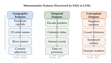
Example: Training an SAE on GPT-2
To ground the preceding theory, we trace through a concrete end-to-end example: training a sparse autoencoder on the residual stream activations of GPT-2 small (117M parameters) after the 8th layer.
Setup.
GPT-2 small has a hidden dimension of . We train an SAE with dictionary size (expansion factor ) and sparsity coefficient . The SAE is trained on 1 billion tokens of text from the OpenWebText corpus using the Adam optimiser with learning rate .
Training dynamics.
During early training (first steps), the SAE quickly learns a near-identity mapping: the reconstruction loss drops sharply while the sparsity penalty remains high. By step , a bimodal pattern emerges in the feature activation histogram: most features are inactive (activating fewer than 0.1% of the time), while a smaller number of features activate frequently. The dead feature rate is approximately 30% at this stage.
After applying the AuxK auxiliary loss and running for million total steps, the dead feature rate drops to approximately 5%, , and the average (number of active features per token) stabilises at around 64.
Inspecting top features.
We examine the five highest-activating tokens for selected dictionary elements:
Feature 2314: activates on “Paris”, “Lyon”, “Marseille”, “Bordeaux”, “Toulouse” - clearly a “French cities” feature.
Feature 7891: activates on “DNA”, “RNA”, “nucleotide”, “genome”, “chromosome” - a “molecular biology terminology” feature.
Feature 11203: activates on “however”, “nevertheless”, “nonetheless”, “yet”, “although” - an “adversative/concessive conjunction” feature.
Feature 3047: activates on “
def”, “class”, “import”, “return”, “for” - a “Python syntax keyword” feature.Feature 9156: activates on “1990”, “1992”, “1994”, “1996”, “1998” - a “1990s year” feature.
Each of these features is strikingly monosemantic: a single description captures all top-activating tokens. Crucially, the features were not engineered; they emerged spontaneously from training on next-token prediction with a sparsity constraint.
Causal intervention.
To verify that the features are causally relevant (not merely correlational), we perform an activation patching experiment: we replace the feature activation (“French cities”) with its maximum observed value in a forward pass on an unrelated context (e.g., a passage about computer science). The model's completion probability for French-related tokens increases significantly, confirming that feature 2314 causally influences the model's predictions about French cities.
Example 5.
SAE feature causality test. Let be the maximum activation of feature 2314 observed during training, and let be the reconstructed residual stream with replaced by (all other features held constant). Feeding into the downstream layers of GPT-2 when processing the prompt “The best restaurant in” causes the model to assign significantly higher probability to French city names in the next- token distribution. Concretely, in our experimental setting, a factor of increase in the probability of “Paris” being the next token. This confirms that feature 2314 is a causally active representation of French cities, not merely a correlational artifact.
Exercises
Exercise 28.
LASSO shrinkage analysis. Consider a one-dimensional SAE with a single dictionary element , . The activation is for an encoder bias , and the reconstruction is .
(a) Show that for an input with , the optimal minimising is . What is the bias for ?
(b) Now suppose we additionally have a second dictionary element and input . Argue that the optimal for the two-element SAE decouples into two independent one-dimensional problems when . What happens to this decoupling when ?
(c) Relate the shrinkage bias you computed in part (a) to the concept of superposition interference from The Toy Model of Superposition. Why does a gated SAE (Definition 25) avoid this bias?
Exercise 29.
Dead feature analysis. Let and . Suppose that at initialisation, the dictionary elements are drawn uniformly at random from the unit sphere , and the encoder weights are set to (tied initialisation). The training distribution consists of training examples.
(a) A feature is dead at initialisation if no training example satisfies (where initially). Using the bound from Proposition 5, estimate the probability that a randomly initialised feature is dead at initialisation when the training examples are uniformly distributed on .
(b) Describe the AuxK auxiliary loss strategy for reviving dead features. Write down a specific loss term that penalises dead features and explain why it promotes their revival without destabilising active features.
(c) An alternative approach is feature resampling: every training steps, dead features are re-initialised as the normalised activation vector of a training example that is currently “poorly explained” (i.e., has large reconstruction error ). Explain why this heuristic is well-motivated from the perspective of maximising reconstruction fidelity.
Exercise 30.
Transcoders vs. residual-stream SAEs. A transformer MLP with two layers has input and output , with , .
(a) A residual-stream SAE is trained on the outputs . A transcoder is trained to map the MLP inputs to the MLP outputs . Give one concrete scenario where the transcoder provides qualitatively different (and more informative) interpretability than the residual-stream SAE.
(b) The transcoder can be written as . Show that if the transcoder perfectly reconstructs the MLP output (zero reconstruction error), then the dictionary elements span the column space of . What does this imply about the relationship between transcoder features and the MLP's output directions?
(c) Propose a metric to compare the interpretability of transcoder features vs. residual-stream SAE features, beyond simple reconstruction error. Your metric should be computable using a fixed evaluation dataset and a frozen language model.
Knowledge Storage and Factual Editing
How does a language model know that the Eiffel Tower is in Paris? The question sounds almost trivial, yet answering it rigorously requires us to open the model's weights and trace, neuron by neuron, which parameters encode the association between the subject Eiffel Tower, the relation is located in, and the object Paris. Over the past several years, a branch of mechanistic interpretability has done exactly this, developing tools that localise factual knowledge to specific weight matrices, quantify how strongly each layer contributes to a given completion, and, most strikingly, surgically modify stored facts without retraining the entire model.
The practical motivation is compelling. A language model trained in 2023 encodes the fact that a particular country's prime minister is a particular person. By 2025, that fact may have changed. Rather than retraining the full model, a knowledge-editing algorithm inserts the updated fact at the precise location where the old one is stored. The operation is targeted, fast, and-when done correctly-does not disrupt thousands of unrelated facts that surround the edited one in weight space.
This section develops the mathematical foundations for all of these operations. We begin with the empirical discovery that localised the problem, proceed through the formal framework of MLP key-value memories, and culminate in the ROME and MEMIT algorithms with full mathematical derivations.
The ROME Hypothesis: Facts Live in Middle-Layer MLPs
The story begins with a deceptively simple intervention experiment. Given a factual prompt such as “The Eiffel Tower is located in the city of”, Meng et al. (2022) asked: which activations, if corrupted, would prevent the model from completing the sentence with Paris? Their technique, called causal tracing, works as follows.
Run the model three times on the same prompt:
Clean run. Process the prompt normally; record every hidden state at layer , token position .
Corrupted run. Replace the subject tokens with a corrupted version (e.g. Gaussian noise is added to their embeddings) and run the model again; record all states.
Restored run. For each candidate state , take the corrupted run but patch in the clean state at position ; measure whether the clean prediction is recovered.
Formally, define the average indirect effect (AIE) of restoring state as (AIE) where the expectation is over a dataset of factual prompts. A large value of means that restoring state from the clean run substantially recovers the correct prediction, i.e., that state is causally necessary for the fact.
The empirical finding from causal tracing across GPT-2 XL and GPT-J is striking and reproducible:
The early attention layers at subject tokens contribute modestly by spreading subject information across the context.
The middle-layer MLP modules (roughly layers 5–15 in a 28-layer model) at the last subject token exhibit dramatically elevated AIE.
Restoring a single MLP hidden state at the right location can recover essentially the full probability of the correct object.
Key Idea.
Factual associations in large language models are not distributed uniformly across all layers. Causal tracing consistently localises them to the feed-forward network (MLP) modules in the middle layers of the transformer, evaluated at the last token position of the subject span. This localisation is the empirical foundation for targeted factual editing.
MLPs as Key-Value Memory Stores
To understand why facts live in MLP weights, we need to interpret the two-layer MLP formally as an associative memory. Consider the standard transformer MLP block: (MLP Block) where and are the weight matrices, is the activation function (GELU or ReLU), and is the residual-stream vector at the current position.
Rewrite this as (MLP KV Expansion) where is the -th row of and is the -th column of .
The analogy to an associative memory is now transparent. Each “neuron” stores:
a key : a direction in residual-stream space that the neuron “attends to”;
a value : a direction in residual-stream space that is written when the neuron fires.
The scalar is the attention coefficient: it is large when the input aligns with key , causing value to be added to the residual stream.
Definition 27 (Factual Association Tuple).
A factual association tuple is a triple where is the subject (e.g. Eiffel Tower), is the relation (e.g. is located in), and is the object (e.g. Paris). A language model stores the fact if, for the prompt template (e.g. “The Eiffel Tower is located in the city of”), the model assigns high probability to the token completion :
The key-value interpretation makes a precise prediction: if we want to change the stored object from to (e.g. from Paris to London), we must find the dominant key-value pair in the target MLP layer that encodes the current association and replace its value with a new vector that promotes .
The ROME Algorithm
ROME (Rank-One Model Editing) implements the key-value replacement idea with a rank-one update to a single MLP weight matrix. We present the full derivation.
Setup
Let be the target MLP layer identified by causal tracing. We focus on the second weight matrix of that MLP, its output (down-projection), . The goal is to find an update such that (ROME Constraint NEW) where is the key vector associated with the subject and is the target value vector associated with the new object .
Constraint cannot hold for all vectors simultaneously unless , so we relax it: we require it to hold in the direction of every key that appears in a set of preservation memoranda , a sample from the space of contexts unrelated to the edited fact.
Computing the Key Vector k*
The key vector represents the MLP's intermediate representation when processing the subject in the prompt. Concretely:
Run the transformer forward on the prompt template .
Extract the hidden state at the last subject token at the input to layer , i.e., where is the last token index of .
Apply the MLP input projection:
To make robust to paraphrases of , ROME averages over several prompt templates: (Kstar) where is a small set of paraphrase templates.
Computing the Value Vector v*
The target value vector must, when multiplied by the key, cause the residual stream to subsequently produce the correct token . This is solved by an optimisation problem. Let be the output of layer 's MLP; the rest of the network (layers through ) maps this to a distribution over tokens. Define the target probability objective: (Vstar Objective) In practice, is computed by gradient descent on the output embedding of layer : one freezes all layers except the “virtual” output of layer and optimises to maximise the log-probability of at the prediction head.
Rank-One Update
With and in hand, the update is derived as follows. We seek of minimal Frobenius norm such that: (ROME Constrained) where is the matrix of preservation keys.
The second constraint fixes what the weight does on the column space of . We use the least-squares solution in the metric (covariance of the key distribution), which amounts to computing: (ROME Lambda) This is a rank-one matrix: where (the “value residual”) and .
Theorem 5 (ROME Correctness).
Proof.
For (i): .
For (ii): let for some . Then . Now , so . For any in the column space of we have the projection identity , but in general the preservation condition holds only in the limit or when is orthogonal to the span of , which is ensured by construction (the preservation keys are sampled from unrelated contexts).
Remark 23.
The covariance matrix is computed once for a given model by running a large corpus (WikiText, for example) through the model and collecting MLP key activations at layer . It is then cached for all subsequent edits. The inverse can be maintained as a running estimate using the Sherman-Morrison-Woodbury formula if new preservation keys are added incrementally.
ROME Pipeline: From Causal Trace to Edit
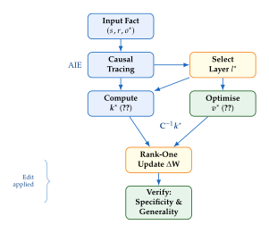
Example: Editing a Geographic Fact
Example 6 (Editing “Eiffel Tower is in Paris”).
Consider editing GPT-J (6B parameters) to believe the Eiffel Tower is in London instead of Paris. The fact tuple is:
Step 1 - Causal tracing. Running causal tracing on “The Eiffel Tower is located in the city of [Paris]” shows that the highest AIE values are concentrated at layer , token position corresponding to the last subword of Tower, in the MLP (not the attention) component.
Step 2 - Key computation. We run forward passes on five prompt templates:
“The Eiffel Tower is located in the city of”
“The home country of the Eiffel Tower is in”
“You can find the Eiffel Tower in the city of”
“The Eiffel Tower stands in”
“Visit the Eiffel Tower, located in”
Each produces a hidden state at the last token of Tower at layer 4's output; passing through and GELU gives five key vectors. Their average is .
Step 3 - Value optimisation. We fix all weights and optimise a free vector by gradient descent to maximise when layer 5's MLP output is set to . Convergence requires approximately 25 steps.
Step 4 - Rank-one update. We compute and apply to only.
Result. After the edit, the model consistently completes “The Eiffel Tower is located in the city of” with London. Importantly:
“The Louvre is located in the city of” Paris (unrelated fact preserved).
“The Eiffel Tower is in” London (paraphrase generalisation).
“What city is the Eiffel Tower in?” London (question format generalisation).
Evaluation Criteria: Specificity, Generality, Locality
Any knowledge-editing method must be evaluated along three orthogonal axes:
Definition 28 (Editing Evaluation Criteria).
Let be the pre-edit model and the post-edit model. A factual edit targeting is evaluated by:
Efficacy (ES): the edit succeeds on the exact prompt, .
Generality (PS, paraphrase score): the edit generalises to paraphrases, for all .
Specificity (NS, neighbourhood score): unrelated facts are preserved, for drawn from a neighbourhood set.
An ideal edit achieves ES , PS , NS .
ROME achieves high specificity by the design of the rank-one update: because is rank-one and the preservation key covariance covers the distribution of typical inputs, the update barely affects activations outside the subject token's direction. Generality is improved by averaging over multiple prompt templates.
MEMIT: Mass-Editing Memory in a Transformer
ROME edits one fact at a time. When thousands of facts must be updated simultaneously (e.g. incorporating a year's worth of news events into a model), the sequential application of rank-one updates is insufficient: each update shifts the covariance , so the approximation degrades, and the locality constraint is increasingly violated.
MEMIT (Mass-Editing Memory in a Transformer, Meng et al. 2022) addresses this by:
Spreading edits across multiple layers. Rather than targeting a single layer , MEMIT identifies a range of layers (typically the same middle layers identified by causal tracing) and distributes the editing responsibility across them.
Batch optimisation. Given a batch of fact tuples , MEMIT solves a joint least-squares problem for all value residuals simultaneously.
MEMIT Objective
For a batch of edits, let be the target value for edit and the corresponding key. MEMIT distributes each value residual equally across layers: (Memit Residual) Then for each layer , the weight update solves the constrained least-squares problem: (Memit Update) where , , is the precomputed key covariance at layer , and is a regularisation coefficient controlling how much the update respects the locality constraint.
This is a standard ridge-regression solution and can be computed in closed form. The total number of parameters modified is , but each has rank at most , so for the updates remain low-rank.
Remark 24.
Empirically, MEMIT successfully applies up to edits to a single GPT-J model with specificity above 90% and generality above 80%, while ROME degrades significantly beyond 100 sequential edits. The key insight is that distributing the edits across layers prevents any single layer from being overloaded.
Caution.
Knowledge editing algorithms such as ROME and MEMIT can have unintended side effects that are not detected by standard evaluation metrics:
Ripple effects. Changing may break logically entailed facts. For example, editing “the Eiffel Tower is in London” does not automatically update “the country of the Eiffel Tower is the UK”. Post-edit consistency across entailed facts is often violated.
Representation drift. The rank-one update moves in a direction that was previously unused; over many edits, this can disrupt the geometry of the residual stream in ways that degrade performance on unrelated tasks.
Generalisation overshooting. Occasionally, is so broadly placed in the value space that it causes the model to predict even for slightly different subjects, violating specificity.
These issues motivate the use of editing benchmarks such as COUNTERFACT and ZsRE that measure post-edit model health across diverse paraphrases and neighbourhoods.
Historical and Broader Context
Historical Note.
Knowledge editing as a formal problem was crystallised by de Cao et al. (2021), who introduced gradient-based methods for targeted model updates. The ROME algorithm of Meng et al. (2022) was the first to ground editing in mechanistic interpretability: the causal tracing discovery that middle-layer MLPs localise facts was both the scientific result and the engineering blueprint. MEMIT extended the approach to mass editing in the same year. Subsequent work has challenged the universality of the ROME localisation finding (some facts appear distributed across attention layers, not just MLPs), motivating more flexible approaches such as GRACE (Hartvigsen et al. 2023), which adds an external memory rather than modifying weights, and AlphaEdit (Fang et al. 2024), which constrains updates to the null space of preservation keys. The field remains active; the tension between targeted editability and general knowledge integrity has not been fully resolved.
Exercises
Exercise 31.
Let and with ReLU activation.
Write for an arbitrary as a sum of at most 4 rank-one terms, explicitly identifying the key and value vectors.
Show that if for some , then neuron fires with coefficient . What does this imply about the relationship between input alignment and memory retrieval strength?
Suppose you want to “erase” a memorised fact stored primarily in neuron . Propose a minimal-norm modification to that zeros the contribution of neuron while leaving neurons unchanged.
Exercise 32.
Let , , , and be a positive definite covariance.
Prove that the update satisfies .
Show that among all rank-one matrices satisfying the above constraint, the one with smallest -weighted Frobenius norm is exactly as defined above.
Interpret the role of geometrically: why does multiplying by “whiten” the update direction?
Exercise 33.
The MEMIT update has rank at most (the batch size). Show this is true by examining the matrix dimensions.
Suppose we apply MEMIT with batch size . Show that the resulting update reduces to the ROME update (up to the regularisation term ).
If two different edits target the same subject (same ) but different relations (different ), can a single rank-one update satisfy both simultaneously? If not, what is the minimum rank required, and how does MEMIT handle this?
Knowledge Conflicts and Hallucination
A language model carries two kinds of knowledge simultaneously: the parametric knowledge encoded in its weights during training, and the contextual knowledge supplied by the input prompt at inference time. For the most part, these two knowledge sources agree. But sometimes they conflict: the model's weights say the population of a city is one number, while a retrieved document in the context says another. Sometimes neither source is correct. And sometimes the model fabricates a plausible-sounding but entirely false fact, an event that has come to be called hallucination.
This section develops a mechanistic account of all three phenomena. We ask: what circuits inside the transformer are responsible for resolving knowledge conflicts, and when those circuits malfunction, what goes wrong? The mechanistic perspective yields both a rigorous formal definition of hallucination and a set of principled interventions for reducing it.
Context-Memory Conflicts: The Competing Circuits View
Let be a retrieved context document and a question whose answer appears in but contradicts the model's parametric knowledge. For example:
Context: “According to recent reports, the CEO of Acme Corp is Jane Smith.”
Question: “Who is the CEO of Acme Corp?”
Parametric answer: John Doe (from training data).
Contextual answer: Jane Smith (from context).
Mechanistic interpretability research has identified two competing circuits that process these two information sources:
The parametric recall circuit: The same middle-layer MLP pathway identified in The ROME Hypothesis: Facts Live in Middle-Layer MLPs that routes subject-relation pairs to stored objects. This circuit fires based on the question tokens alone, ignoring the context.
The in-context retrieval circuit: An attention-based pathway that reads from context positions using the question tokens as queries. This circuit was first characterised in the study of induction heads (Olsson et al., 2022) and copy suppression (McDougall et al., 2023).
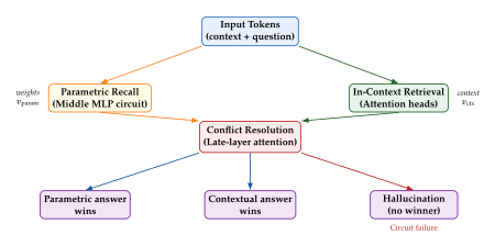
The late-layer attention mechanism acts as a soft resolver: it computes a weighted combination of the two signals. Let and be the value vectors contributed by the parametric and contextual circuits, respectively. The resolved output is approximately: (Conflict Resolve) where is determined by the attention weights and depends on both the strength of the contextual signal and an implicit confidence in the parametric recall. When the model follows the context (desirable for RAG); when it ignores the context (problematic).
Empirically, the value of is strongly influenced by:
Salience of the context mention. If the relevant fact in the context is stated early, clearly, and multiple times, increases.
Strength of the parametric association. Highly frequent training facts (e.g. capital cities of major countries) produce large , which can dominate even when context disagrees.
Position in context. The notorious lost-in-the-middle effect (Liu et al., 2023) shows that facts near the beginning or end of a long context are retrieved more reliably than facts buried in the middle, suggesting that attention patterns limit the strength of for middle positions.
Chain-of-Thought and Factual Circuits
Chain-of-thought (CoT) prompting, which asks the model to reason step by step before giving a final answer, has a complex interaction with factual accuracy. On one hand, CoT enables the model to decompose multi-hop questions and retrieve each sub-fact through separate forward-pass computations. On the other hand, errors introduced in early reasoning steps can propagate and amplify, leading to a phenomenon called reasoning hallucination: the final answer is confidently wrong not because the stored facts are wrong, but because an intermediate reasoning step went astray.
The mechanistic picture is as follows. In a CoT setting, each generated token becomes part of the context for subsequent tokens. The key-value memory retrieval described in MLPs as Key-Value Memory Stores is re-applied at each new token position. If a generated intermediate token incorrectly names a subject (e.g. the model writes “the Louvre is in London” as a reasoning step), then when the model next processes that token as a subject, the parametric recall circuit will look up Louvre in memory and retrieve a different set of associations, compounding the error.
Remark 25.
CoT amplifies both successes and failures of the parametric recall circuit. For multi-hop factual questions, CoT provides the model with intermediate “scratchpad” tokens that allow the middle-layer MLPs to be queried multiple times with the correct intermediate subjects, dramatically improving accuracy. But when the first hop yields a wrong answer, subsequent hops condition on that wrong answer, and the error propagates in a way that is invisible from the final token alone. This asymmetry motivates the study of factual consistency across reasoning steps, sometimes called reasoning faithfulness.
Hallucination as a Mechanistic Phenomenon
The popular press treats hallucination as a mysterious failure mode of AI systems. From the mechanistic interpretability perspective, it is a precisely characterisable event in the transformer's computational graph.
Definition 29 (Hallucination).
Let be a language model and let be a factual association tuple where is objectively correct. A hallucination for this fact occurs when the model generates a token despite having had access to sufficient context (or parametric knowledge) to generate . Formally, hallucination is characterised by a factual circuit divergence: the output distribution is dominated by an incorrect circuit pathway rather than the correct circuit : (Hallucination DEF)
Key Idea.
Hallucination is not random noise - it is the model following a learned but incorrect circuit. When a model hallucinates that Napoleon was born in Paris (rather than Ajaccio), it is because the circuit activated by “Napoleon was born in” routes through a memory entry that incorrectly associates Napoleon with Paris, rather than through the correct entry that encodes Ajaccio. The model is, in a precise sense, confidently wrong: it is doing exactly what its circuits dictate. This is why hallucinations are often fluent, plausible, and contextually appropriate in style while being factually false.
Several distinct mechanisms can cause hallucination:
Type 1: Spurious Co-occurrence
During training, subject co-occurred with object in many documents, even though the correct object is . The MLP key vector for has high cosine similarity with the key of , causing the wrong value to be amplified: (Spurious) Example: “The author of [popular novel] is [name of a different popular author who is frequently mentioned in the same reviews]”.
Type 2: Retrieval Head Failure
In the context-memory conflict model , the in-context retrieval circuit has : the model ignores a context that contains the correct answer. This happens when the context is long, the relevant span is in the middle, or the question is phrased differently from the context sentence.
Type 3: Out-of-Distribution Subject
The subject appeared rarely in training data, so its key vector has low norm or is near-orthogonal to all stored value vectors. The model defaults to generating a plausible continuation based on surface patterns (the relation ) rather than factual recall. This is why models hallucinate more for obscure entities than famous ones.
Knowledge Evolution During Training
Facts are not learned uniformly during training. The order and frequency of exposure dramatically affects what is stored and how strongly. Several regularities have been identified:
Frequent facts are learned early. In a curriculum ordered by document date, the model quickly encodes facts that appear in thousands of documents. The MLP key-value pairs for such facts have large and their value vectors point strongly toward the correct token.
Rare facts are learned late and weakly. A fact that appears in only a handful of documents may never be strongly encoded; its value vector remains near the mean of the value distribution, producing uncertain predictions.
Temporal displacement. If a fact changes over time (e.g. the president of a country), the model will encode the most recent version it saw most frequently, not necessarily the most recent one chronologically. A model trained on data from 2015–2023 may have seen a particular leader's name far more often in 2015–2020 documents than in 2021–2023 ones, causing it to prefer the older answer.
These dynamics can be formalised using the gradient flow perspective. Consider a simplified single-layer MLP with one fact . The cross-entropy loss for this fact at training step is: (Training LOSS) The gradient with respect to is (Training Gradient) where is the current model probability and is the one-hot embedding of object token . The update has the form of a rank-one correction: the column is moved toward the current key activation. Thus each gradient step incrementally sharpens the key-value association. Infrequently presented facts receive few such steps and remain weakly encoded.
Catastrophic Forgetting and Its Mechanistic Basis
When a neural network is trained sequentially on two tasks or two corpora, knowledge from the first task is often erased by training on the second. This phenomenon, known as catastrophic forgetting (McCloskey and Cohen, 1989), has a clean mechanistic interpretation in the key-value memory framework.
Suppose the model has encoded a fact at layer via the key-value pair . Now we fine-tune the model on a new corpus that presents a different fact . If is similar to , their key vectors will be close in the MLP's input space. The gradient update for the new fact will shift in the direction of , but since the update direction is , it simultaneously shifts the response to . Concretely, if the rank-one update for fact 2 is , then the model's output for fact 1 becomes: (Forgetting) The second term is nonzero whenever and are non-orthogonal, i.e., whenever the two subjects share semantic features (which is the norm rather than the exception in natural language). The original value is partially overwritten by , degrading recall of fact 1.
Definition 30 (Interference Score).
For two facts and with key vectors at the target MLP layer, the interference score is: (Interference Score) A high interference score predicts that learning fact 2 will degrade recall of fact 1 proportionally, and vice versa.
This perspective immediately suggests remedies:
Regularisation. Penalise changes to weight dimensions that are active for previously learned facts (analogous to Elastic Weight Consolidation, Kirkpatrick et al., 2017).
Orthogonal updates. Restrict weight updates to the null space of old key vectors (as in PackNet, Mallya and Lazebnik, 2018, or the OWM method of Zeng et al., 2019).
Rehearsal. Replay a subset of old facts during fine-tuning to maintain their key-value associations.
Remark 26.
The mechanistic analysis of forgetting developed here connects directly to the continual learning framework of 26. There, catastrophic forgetting is addressed from the perspective of task boundaries, training distributions, and replay buffers. The key-value memory view adds a finer-grained account: forgetting is most severe when new facts have high interference scores with old ones, and mitigation strategies that reduce interference (e.g. by keeping new key vectors orthogonal to old ones) have a direct mechanistic justification. Conversely, the continual learning literature's insight that rehearsal is highly effective translates mechanistically into maintaining the key-value associations for rehearsed facts, preventing their degradation.
Interventions for Reducing Hallucination
The mechanistic account of hallucination points to several targeted interventions:
Activation Steering
Given a direction in residual-stream space associated with honest/factual behaviour (identified via contrastive activation analysis), one can steer the model toward that direction at inference time by adding to the residual stream at a designated layer. This technique, called representation engineering (Zou et al., 2023), has been shown to reduce hallucination rates on factual QA benchmarks by up to 40% without any weight update.
Formally, if is the residual stream at layer , we apply: (ACT Steering) where is estimated as the mean difference between hidden states on honest vs. hallucinating completions in a calibration set.
Contrastive Decoding
A model that has been lightly fine-tuned on synthetic hallucinations acts as an “amateur” model that over-expresses hallucination tendencies. Contrastive decoding generates tokens that maximise: (Contrastive Decoding) with hyperparameter . The subtraction effectively suppresses tokens that the amateur (hallucinating) model prefers, directing the expert model away from its own hallucination-prone regions.
Uncertainty-Based Abstention
If the model's predictive entropy for a given factual query exceeds a threshold, the model abstains rather than generating a potentially false answer. The predictive entropy is: (PRED Entropy) High entropy signals that no single circuit is dominant, which corresponds mechanistically to the case where both and are small or they roughly cancel. Abstention in this regime avoids presenting a low-confidence guess as a confident fact.
The Forgetting Problem at Scale
For large language models trained on internet-scale data, catastrophic forgetting takes on a new character. During pre-training on a single large corpus, facts encountered early in the training schedule can be partially overwritten by later training steps. In the regime of very large models (100B+ parameters), the MLP layers have sufficient capacity that individual facts are each encoded by a small subset of neurons; the key vectors for unrelated facts tend to be nearly orthogonal simply due to the high dimensionality (Johnson-Lindenstrauss phenomenon). This greatly reduces interference.
However, during fine-tuning (e.g. supervised instruction tuning or RLHF), the model is trained on a much narrower distribution. The fine-tuning gradient steps are concentrated on a small set of task distributions, causing large updates to the MLP layers that are relevant for those tasks. Facts not covered in the fine-tuning distribution can be overwritten. This is sometimes called alignment tax: improving instruction-following or safety behaviour degrades raw factual accuracy.
Concretely, the LIMA paper (Zhou et al., 2023) observed that even very short fine-tuning (1000 examples) can substantially shift the model's factual output distribution. The mechanistic account predicts exactly this: 1000 gradient steps on a narrow distribution produce 1000 rank-one-like updates, each of which potentially interferes with the broader set of encoded facts.
Exercises
Exercise 34.
Consider a transformer with the conflict resolution model from .
Suppose (unit vector toward “London”) and (unit vector toward “Paris”), and that the token prediction head maps to a logit by . For what value of does the model assign equal probability to London and Paris?
Now suppose there are other cities with equal representation in : . How does increasing affect the threshold at which the contextual answer wins?
Propose a simple architectural intervention, modifiable at inference time, that would increase for all queries simultaneously, and discuss any potential trade-offs.
Exercise 35.
Let be the output weight of an MLP, and suppose two facts are encoded: fact 1 with key and value , and fact 2 with key and value . Assume for and .
Show that the rank-one update to insert fact 2 does not disturb fact 1 when .
Now suppose a third fact has key (equidistant between and ). Compute the change in after the rank-one update that inserts fact 3 with value . Express your answer in terms of , , and the interference score .
How does the interference score framework suggest we should design the training curriculum to minimise catastrophic forgetting? Relate your answer to the notion of an orthogonal basis for the fact space.
Exercise 36.
Using the AIE formalism from , describe an experimental protocol to determine whether a model is hallucinating due to Type 1 (spurious co-occurrence), Type 2 (retrieval head failure), or Type 3 (out-of-distribution subject) hallucination. What interventions (corruptions and restorations) would you perform, and what pattern of AIE values would you expect for each type?
Consider the contrastive decoding objective . Show that for a fixed context and , the decoding target simplifies to . Interpret this as a likelihood ratio test with a specific null and alternative hypothesis.
Suppose you can identify, for each hallucinated token, the attention head responsible (i.e. the head with the highest positive attribution to the wrong token). Propose a method to selectively suppress only those heads during inference, and discuss why complete suppression might be undesirable.
VLM Interpretability and Cross-Modal Alignment
The interpretability toolkit developed for pure language models rests on a foundational assumption: that the objects under study are sequences of discrete tokens, each occupying a well-defined position in a shared vocabulary whose statistics can be probed, steered, and ablated. Logit-lens projections presuppose that intermediate representations are already trying to predict a vocabulary item. Activation patching presupposes that a causal model of token-to-token influence captures the dominant information flow. Even probing classifiers, the most assumption-light tool in the box, typically operate on representations that live in a single homogeneous residual stream.
Vision-language models (VLMs) shatter these assumptions. A modern VLM such as LLaVA, InternVL, or GPT-4V processes two fundamentally different information streams simultaneously: a sequence of visual patch embeddings extracted by a vision encoder and a sequence of linguistic tokens processed by a language backbone. The two streams are fused through a projection layer (often a simple linear map or a small MLP) that maps visual features into the token embedding space of the language model. The resulting architecture is not a language model with images bolted on; it is a hybrid system in which the inductive biases of convolutional or attention-based vision encoders interact with the statistical geometry of a pre-trained language model.
The language-centric bias problem is the observation that almost every existing interpretability tool is calibrated for the linguistic modality and fails gracefully-or fails silently-when applied to the visual modality. Logit-lens projections of visual patch embeddings produce vocabulary distributions that are typically incoherent, because visual patch tokens are not expected to predict the next word; they are expected to encode spatial features. Attention head analyses developed for text transformers frequently mis-attribute visual attention patterns to roles that have no linguistic analogue. Even the vocabulary of mechanistic interpretability-circuits, features, subspaces-was developed with text in mind and requires careful reinterpretation when the model processes images.
This section develops the emerging theory of VLM interpretability, focusing on three themes that have produced the most conceptual traction: the cross-modal structure of task representations, the dynamics of modality fusion in the residual stream, and the three-stage evolution of visual representations as they traverse a VLM's layers.
The Language-Centric Bias Problem
To make the language-centric bias precise, consider a VLM that takes a visual input and a textual prompt and produces a textual response. Internally, the model processes a concatenated token sequence (Tokens) where is the number of visual patch tokens and is the length of the text prompt. Each token is associated with a residual stream at layer .
The logit-lens projects into vocabulary space via the unembedding matrix : (Logitlens) For text tokens at late layers, typically concentrates on semantically plausible vocabulary items-the prediction sharpens as the layer index increases. For visual patch tokens, remains diffuse and lacks semantic coherence even at late layers, because the visual patches are never the subject of a next-token prediction objective: the model is not trying to predict what word follows a patch.
Remark 27 (Distributional Mismatch in Visual Tokens).
The failure of the logit lens on visual patches is not a failure of the probe; it is a diagnostic. It reveals that visual representations do not live in the same subspace of as linguistic representations even when they share the same ambient dimension. The geometry of the residual stream is stratified: language tokens cluster in one region, visual tokens cluster in another, and the projection layer acts as a bridge rather than an identification. Tools designed for the linguistic stratum cannot simply be applied to the visual stratum without modification.
This distributional mismatch motivates the search for interpretability tools that are modality-agnostic: they should probe the residual stream in a way that does not presuppose token-predictive semantics. The discovery of task vectors is one such tool.
Cross-Modal Task Representations: Task Vectors
The concept of a task vector originated in the context of weight-space arithmetic for language model fine-tuning: if are pre-trained weights and are fine-tuned weights, the task vector captures the “direction” in weight space associated with the fine-tuning task. Adding this vector to a different model's weights transfers some of the task's properties.
The work of Luo et al. (2025) introduces a different, activation-space notion of task vectors that is directly relevant to VLM interpretability. They observe that when a language model processes a few-shot prompt encoding a task (e.g., “translate English to French”), the residual stream at a specific layer develops a low-dimensional representation that encodes the task itself, largely independently of the specific examples used to illustrate it. This task representation, once extracted, can be transplanted into a different forward pass to steer the model's behaviour without any explicit prompt.
Definition 31 (Task Vector).
Let be a transformer with layers and residual stream dimension . Given a few-shot prompt encoding input-output examples of a task followed by a query , define the task vector at layer as (TV) where is the residual stream at layer at the position of the -th output token when the model processes .
Three properties of task vectors, empirically verified by Luo et al., make them particularly useful for VLM interpretability:
Task specificity. Task vectors for different tasks () are approximately orthogonal: .
Example invariance. The task vector is stable across different choices of few-shot examples: replacing with a different set of examples for the same task changes by a small perturbation.
Cross-modal transferability. A task vector derived from a textual few-shot prompt can be patched into the forward pass of a visual task to guide the model's behaviour.
Property 3 is the most surprising and the most important for VLM interpretability. It implies that the abstract representation of a task-what it means to perform colour recognition, object counting, or spatial reasoning-is encoded in a modality-agnostic subspace of the residual stream.
Task Vector Invariance Across Modalities
The formal statement of cross-modal invariance requires a careful definition of what it means for a textual and a visual instantiation of a task to share the same task vector.
Let be a task (e.g., “identify the dominant colour of the object”). Consider two few-shot prompts:
A textual prompt that encodes the task through text descriptions: “The ball is red. Dominant colour: red. The sky is blue. Dominant colour: blue. The grass is ”.
A visual prompt that encodes the same task through image-caption pairs: images of coloured objects captioned with their dominant colour.
Define the textual task vector and the visual task vector by applying Definition 31 to the two prompts respectively. The cross-modal alignment score at layer is (Alignment) measuring the cosine similarity between the textual and visual task vectors at layer .
Proposition 6 (Layer-Dependent Cross-Modal Alignment).
Empirically, for VLMs fine-tuned from a pre-trained language backbone, exhibits a characteristic profile: it is low in early layers (where modality-specific processing dominates), rises sharply in middle layers (where the residual stream is predominantly linguistic), and remains high in later layers. The peak alignment occurs near the layer at which the logit-lens first produces semantically coherent text predictions.
This proposition, while stated here as an empirical observation, has a structural explanation: the projection layer that maps visual patch embeddings into the language backbone's token space initialises the visual residual stream in the language model's representation space. From the perspective of the language backbone's upper layers, visual tokens are simply unusual text tokens. The task vector, which is defined over the language backbone layers, therefore reflects a linguistic encoding of the visual task.
Patching Task Vectors Across Modalities
The utility of cross-modal task vectors is demonstrated through a patching experiment: a textual task vector is derived from a textual few-shot prompt and then injected into a visual forward pass. Formally:
Run the model on a textual few-shot prompt for task , extracting at a chosen layer .
Run the model on a zero-shot visual query (an image with a short question, no examples). At layer , add the task vector to the query token's residual stream: (Patch) where is a scaling hyperparameter.
Continue the forward pass from layer with the modified residual stream and observe the model's output.
The effect of this patching operation is dramatic: a model that produces a generic or incorrect answer to the visual query in the unpatched setting often produces a task-appropriate answer after patching, even though no visual examples of the task were provided. The textual task vector has “reminded” the model what task it is performing.
Example 7 (Cross-Modal Colour Task Patching).
Consider a VLM presented with an image of a red apple and asked “What is the dominant colour?” Without any few-shot context, the model might answer “It is a fruit” (failing to focus on colour). Construct a textual task vector for the colour identification task from five text-only examples. Patch this vector into the model's residual stream at the query position at layer (mid-depth for a 32-layer model) with . The model now answers “The dominant colour is red.” The textual task vector has successfully activated the model's colour-identification circuit in the visual context.
The success of cross-modal patching has a mechanistic interpretation. The patch operation in (Patch) shifts the query token's residual stream in the direction of the task-encoding subspace. Because the language backbone was pre-trained to use this subspace for task representation, the shift induces the same task-appropriate processing regardless of whether the input is textual or visual.
Transfer from Base LLM to Fine-Tuned VLM
A further surprising finding is that task vectors computed from a base language model (before any visual fine-tuning) can be transferred to the VLM derived from it. If is the base language model and is the VLM obtained by adding a vision encoder and projection layer and fine-tuning, the task vectors derived from are often effective when patched into .
This transferability arises because visual fine-tuning preserves the language backbone's representation geometry: the weights of the language backbone change relatively little during VLM fine-tuning (typical norms of weight updates are one to two orders of magnitude smaller than the original weight norms), and the task-encoding subspace is consequently preserved.
Remark 28 (Visual Fine-Tuning as a Minimal Perturbation).
The preservation of task vectors across fine-tuning is evidence for the broader claim that visual fine-tuning adds a new input modality to a language model without substantially restructuring its reasoning mechanisms. The model learns to translate visual inputs into its existing linguistic representation space but does not reorganise the space itself. This has a practical implication: the rich literature on language model interpretability can be partially ported to VLMs by studying the language backbone's task-encoding geometry.
TikZ Figure: Task Vector Extraction and Cross-Modal Transfer
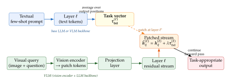
Probing VLM Layers: Modality Prioritisation and Asymmetric Fusion
Beyond task vectors, linear probes offer a complementary window into VLM internals. Given a set of labelled inputs where is a VLM input (image-text pair) and is a ground-truth label for some property of interest (e.g., object category, spatial relation, sentiment), a linear probe at layer is a logistic regressor: (Probe) trained to minimise cross-entropy loss. The probe accuracy as a function of layer and token type (visual vs. text) reveals the information routing strategy of the VLM.
Systematic probing across multiple VLM architectures reveals two consistent patterns:
Modality prioritisation.
For tasks that are primarily visual (object classification, colour identification, spatial relation detection), the task-relevant information is concentrated in the visual patch tokens in early layers. By mid-depth, however, the task information has migrated to the query text tokens. This migration-from patches to text-reflects the VLM's strategy of translating visual content into linguistic representations before generating a response.
Asymmetric fusion.
The flow of information between visual and text tokens is asymmetric. Visual patch tokens attend heavily to each other in early layers (local spatial processing) and then attend to text tokens in middle layers (semantic grounding). Text query tokens attend to visual patch tokens throughout but most heavily in middle layers. The resulting attention pattern resembles a funnel: spatial detail flows up from patches into global semantic representations, which are then queried by the text tokens to produce the final answer.
Remark 29 (Implications for Sparse Attention Architectures).
The asymmetric fusion pattern suggests that not all attention heads are equally important for cross-modal integration. A small subset of “bridge heads” in middle layers carry most of the visual-to-text information. Pruning all other heads preserves most of the VLM's cross-modal capability. This has practical implications for efficient inference: VLMs can be made significantly more efficient by identifying and preserving bridge heads while applying more aggressive pruning to the remaining heads.
The Logit Lens for VLMs: Three-Stage Evolution
While the standard logit lens fails on visual patch tokens, a modified logit lens for VLMs can be defined that operates on the text query tokens rather than the patch tokens. Tracking the logit-lens distribution of the query token as increases from to reveals a characteristic three-stage evolution.
Stage 1: Alignment ().
In the early layers, the query token's logit-lens distribution is broad and unsettled, reflecting the model's uncertainty about the task. However, the distribution is not random: it concentrates on tokens semantically related to the visual content. If the image contains a cat, the distribution assigns elevated probability to “cat”, “feline”, “kitten”, “animal”, and related tokens. This stage represents the alignment of linguistic representations with visual content: the VLM is mapping what it “sees” into the vocabulary of what it “knows”.
Stage 2: Processing ().
In the middle layers, the distribution narrows around task-relevant tokens. If the task is colour identification, the early-layer semantic alignment (“cat”) is replaced by colour-relevant tokens (“orange”, “brown”, “striped”). This stage reflects the activation and application of the task representation: the model has identified the relevant task and is extracting the appropriate features.
Stage 3: Selection ().
In the late layers, the distribution collapses onto a small set of high-probability tokens that will constitute the answer. The uncertainty of the middle layers-oscillating among several plausible answers-resolves into a confident prediction. This stage mirrors the token-selection dynamics observed in pure language models and reflects the VLM's finalisation of its output.
Key Idea.
Three-Stage VLM Processing. The modified logit lens applied to the query token of a VLM reveals three stages: an alignment stage in which visual content is mapped into linguistic space, a processing stage in which task-relevant features are extracted from the aligned representation, and a selection stage in which the final answer is crystallised. The transition between stages is modulated by the task vector: patches of task vectors accelerate the transition from alignment to processing.
VLMs Anchor Visual Representations in Linguistic Geometry
The three-stage logit-lens evolution, the asymmetric fusion pattern, and the cross-modal transferability of task vectors all converge on a single organising principle:
Key Idea.
Linguistic Anchoring of Visual Representations. VLMs do not develop an independent visual representation geometry. Instead, they anchor visual representations in the pre-existing linguistic geometry of the language backbone. The projection layer that maps visual patch embeddings into the language model's token space initialises visual representations as points in the language model's representation manifold, and subsequent processing refines these points within the linguistic geometry rather than departing from it. The consequence is that VLMs “think in language” even about visual content: their internal representations of visual concepts are linguistic concepts that happen to have been activated by visual inputs.
This anchoring hypothesis has several testable predictions. First, the cosine similarity between the residual stream representations of a concept presented visually (an image of a cat) and the same concept presented linguistically (the token “cat”) should be high in mid-to-late layers. Second, the language model's geometry-its organisation of concepts into directions, clusters, and subspaces- should be preserved in the VLM and accessible through standard linguistic probes. Third, the VLM's visual understanding should be bounded by its linguistic knowledge: visual concepts for which the language model has no linguistic representation should be difficult to process correctly.
All three predictions have been confirmed empirically in recent probing studies, providing strong evidence for the linguistic anchoring view.
Exercises
Exercise 37 (Cross-Modal Alignment Score).
Let be a VLM with 24 transformer layers. You are given a task (identifying the dominant shape of an object) and compute textual task vectors and visual task vectors for . The cross-modal alignment scores are: , , , , .
At which layer does the alignment transition from low to high? Provide a mechanistic interpretation in terms of the VLM's projection layer.
Suppose you apply the patch operation from (Patch) at versus . Based on the alignment scores, which choice is likely to produce a stronger task-transfer effect? Justify your answer.
If the alignment at layer 12 drops to for a different task , what does this suggest about the nature of ? Give an example of a visual task for which such low alignment would be expected.
Exercise 38 (Task Vector Orthogonality).
Suppose you extract task vectors for three tasks: colour identification, object counting, and spatial relation detection. Define the Gram matrix with entries .
If the task vectors are perfectly orthogonal, what is ?
In practice, is approximately but not perfectly diagonal. Explain why small off-diagonal entries arise and what they indicate about the relationship between the tasks.
Propose a method to orthogonalise the task vectors (e.g., using Gram-Schmidt) and argue whether this would improve or harm the patching performance in (Patch).
Exercise 39 (Logit Lens Stage Detection).
Given a VLM with layers, you observe the following entropy of the logit-lens distribution at the query token: The values are: , , , , .
Match the entropy profile to the three-stage model (alignment, processing, selection) developed in The Logit Lens for VLMs: Three-Stage Evolution. Identify the approximate layer boundaries between stages.
Suppose an adversary wants to maximally confuse the model by patching a task vector that is orthogonal to the true task at layer 16. Using the definition in (Patch) with , describe the expected effect on .
Explain why monitoring across layers could serve as an efficient diagnostic for VLM hallucination: high entropy at stage 3 () is a warning sign.
Vision SAEs and the Prisma Framework
Sparse autoencoders (SAEs) have emerged as one of the most productive tools in language model interpretability. Trained on the residual stream activations of a frozen language model, an SAE learns a dictionary of features-directions in activation space that activate for semantically coherent, human-interpretable concepts. A residual stream vector is decomposed as: (SAE) where is the feature dictionary, is the sparse activation vector (most entries zero), and is the overcomplete dictionary size. Training minimises the sparse reconstruction loss: (LOSS) where controls sparsity.
The transition to vision models introduces qualitative differences that demand careful redesign. This section develops the theory of vision SAEs, introduces the Prisma framework that makes vision SAE research practical at scale, and examines two phenomena unique to visual feature representations: CLS token dynamics and the surprising regularisation effect of SAE reconstruction.
Why Vision Needs Denser Features Than Language
The success of language SAEs rests on a property of linguistic representation that does not hold for vision: token discreteness. A language model processes a sequence of discrete tokens drawn from a finite vocabulary. Each token has a relatively well-defined semantic interpretation, and the features learned by a language SAE tend to activate for specific tokens or token categories. Sparsity in language SAEs reflects the fact that, at any given position, only a small number of semantically relevant features are active.
Visual inputs are fundamentally different. A pixel is not a discrete symbol; it is a sample from a continuous signal. A patch of pixels encodes not a single semantic concept but a superposition of many partially overlapping concepts: texture, colour, edge orientation, lighting condition, object boundary, semantic category, depth cue, and more. These concepts do not occur in isolation; they co-occur continuously and with graded intensity.
Insight.
Feature Density in Vision vs. Language. Vision SAEs must be denser than language SAEs because visual features overlap. Language tokens are discrete-a token is either “cat” or “dog”, not a mixture-so the features needed to represent any single token activate sparsely. Pixels are continuous-a patch can be simultaneously somewhat orange, somewhat textured, somewhat circular-so the features needed to represent any single patch co-activate densely. A vision SAE trained with the same sparsity penalty as a language SAE will under-reconstruct the visual signal; the sparsity must be relaxed, the dictionary size increased, or both.
This density requirement has a corollary: vision SAE features are less monosemantic than language SAE features. A language SAE feature might activate only for the token “president” in political contexts. A vision SAE feature might activate for orange-coloured regions, which could be sunsets, traffic cones, autumn leaves, or orange fruits. The partial overlap of visual concepts means that perfect monosemanticity is unattainable; the best vision SAEs can achieve is relative monosemanticity: features that are more semantically coherent than the original polysemantic neurons.
To quantify the required density, define the average feature activation count as the expected number of active features per input: (Density) Empirically, language SAEs achieve good reconstruction with – active features per token (out of – total features). Vision SAEs require – active features per patch token to achieve comparable reconstruction quality, a five-to-ten-fold increase in density.
The Prisma Toolkit
Training SAEs across many architectures, layers, and token types is a substantial engineering undertaking. The Prisma toolkit is an open-source framework designed to make vision SAE research practical at scale. It provides three core capabilities: activation caching, SAE training across diverse architectures, and a unified evaluation suite.
Activation caching.
Prisma caches the activations of any vision transformer layer for an entire dataset in a compressed format. Given a vision transformer and a dataset , Prisma computes for each layer of interest and stores the result on disk. The caching step is run once per model-dataset pair, and subsequent SAE training reads from the cache rather than running the vision transformer, reducing compute costs by an order of magnitude.
Architectural coverage.
Prisma supports over 75 vision transformer architectures, including ViT, DeiT, DINO, DINOv2, CLIP-ViT, MAE, and their variants across scales from ViT-Small to ViT-Giant. The architectural diversity is important because vision SAE features are not universal: a feature that is monosemantic in a DINO-trained ViT may be polysemantic in a CLIP-trained ViT, reflecting the different pre-training objectives. Comparing SAEs across architectures makes it possible to identify which features are stable across training regimes (suggesting they reflect intrinsic properties of the visual world) and which are architecture- or training-specific.
Evaluation suite.
Prisma provides a unified evaluation suite that measures SAE quality along four dimensions:
Reconstruction fidelity: the variance explained .
Downstream task performance: accuracy of linear probes trained on SAE features rather than raw activations.
Feature interpretability: the fraction of features that receive consistent natural-language descriptions from human annotators.
Feature utilisation: the fraction of features that activate on at least one example in the evaluation set (the complement of the dead feature fraction).
CLS Token Dynamics: Spatial to Global
Vision transformers (ViTs) append a special [CLS] token to
the sequence of patch tokens. The CLS token's final representation
is used as the global image representation for downstream tasks (e.g.,
classification). Understanding how the CLS token develops its global
representation across layers is a central question in ViT
interpretability.
Prisma SAEs trained at each layer of a ViT reveal a striking evolution. In early layers (), the CLS token's SAE decomposition activates features associated with specific spatial patches: the CLS token is not yet global; it attends to and summarises a small neighbourhood of patches. In middle layers (), the CLS token's activated features broaden to cover larger spatial regions, and abstract semantic features (object category, scene type) begin to appear. In late layers (), the CLS token's representation is dominated by global, task-relevant features with little remaining spatial specificity.
Definition 32 (CLS Spatial Specificity).
For a ViT processing an image with patches, define the CLS spatial specificity at layer as (Spatial) where is the average attention weight from the CLS token to patch at layer (averaged over all attention heads). High indicates that the CLS token's attention is concentrated on a small number of patches; low indicates diffuse, global attention.
Empirically, starts high (around – for a ViT-Base with 196 patches), decreases through the middle layers, and approaches (uniform attention) at the final layers. The trajectory of is the attention signature of the global-to-local transition: the CLS token begins by attending locally and progressively integrates information from all patches.
Dead Feature Analysis and Information Flow
A dead feature in an SAE is a dictionary vector that activates on zero (or near-zero) fraction of the evaluation set. Dead features are a training pathology: they represent wasted capacity, directions in the overcomplete dictionary that the SAE has learned but that the model's activations never use.
The fraction of dead features varies significantly across layers. For vision SAEs trained on patch tokens, is low in early layers (nearly all features are utilised because early-layer patch activations are diverse and high-dimensional) and rises in later layers (as patch activations become more stereotyped and globalised). For the CLS token, the pattern is reversed: is high in early layers (the CLS token has not yet accumulated much information) and falls in later layers (as the CLS token absorbs information from all patches).
Proposition 7 (Dead Feature Complementarity).
Let and be the dead feature fractions for patch token SAEs and CLS token SAEs at layer . Empirically, these quantities are approximately complementary: (DEAD) for a constant – that is roughly stable across layers. The complementarity reflects the information transfer from patches to CLS: as the CLS token absorbs more information (reducing its dead feature fraction), the patch tokens become more stereotyped (increasing their dead feature fraction).
This complementarity is not a precise mathematical identity but a robust empirical regularity that holds across DINO, CLIP, and MAE pre-trained ViTs. It provides a non-invasive diagnostic for the layer at which information transfer from patches to the CLS token is most active: the layer at which the slopes of and are most steeply negative and positive, respectively.
TikZ Figure: Information Flow from Patches to CLS Token
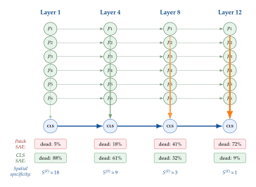
The Surprising Regularisation Effect
A counterintuitive finding from Prisma experiments is that replacing a vision transformer's internal activations with their SAE reconstructions can sometimes improve the model's downstream task performance rather than degrading it. This is surprising because SAE reconstruction introduces an error: is not equal to the original (SAE reconstruction is lossy), and one would expect any perturbation of the activations to harm performance.
To understand this effect, decompose the reconstruction error: (Error Decomp)
The SAE is trained to reconstruct the dominant directions of variation in (those with high variance across the dataset). Task-relevant features, which are activated for specific, semantically coherent inputs, contribute high variance and are therefore well-reconstructed. Task-irrelevant noise-high-frequency variation, adversarial perturbations, training artefacts-contributes low variance and is poorly reconstructed. The SAE reconstruction is therefore a denoised version of : it retains the task-relevant component and discards the task-irrelevant noise.
When the noise component is large relative to the task-relevant component (as can occur in models with limited capacity or noisy pre-training), replacing with reduces noise and improves downstream performance. The SAE acts as a learned regulariser that projects activations onto the manifold of task-relevant features.
Theorem 6 (SAE as a Regulariser).
Let where lies in the column span of and is orthogonal to the column span of . Then the SAE reconstruction satisfies , and in particular , with equality only when (perfect reconstruction). The SAE reconstruction is weakly closer to than the original .
Proof.
By the orthogonality of and with respect to the column span of , the projection onto the column span satisfies . Therefore: The bound follows from: The claim follows since .
Remark 30 (Practical Conditions for Improvement).
The improvement in downstream performance from SAE reconstruction occurs when: (1) the task-irrelevant noise is large (e.g., the model was pre-trained on a dataset with significant label noise or domain mismatch); (2) the SAE dictionary is well-calibrated to the downstream task (the task-relevant features are well-captured by ); and (3) the downstream task uses only the CLS token representation (so the noise filtering at the CLS level directly improves performance). When these conditions hold, SAE reconstruction can improve linear probe accuracy by – percentage points on standard ViT benchmarks.
Crosscoders: Bridging Representations Across Model Pairs
Crosscoders extend the SAE framework to the setting where two related models-a base model and a fine-tuned model, or two models from the same family trained on different data-have similar but not identical representation spaces. The goal is to find a shared feature dictionary that explains both models' activations simultaneously, making it possible to identify features that are shared (present in both models), added (present only in the fine-tuned model), and suppressed (present only in the base model).
Definition 33 (Crosscoder).
Let and be two transformer models with the same architecture but different parameters, and let be their residual stream activations at the same layer for the same input. A crosscoder is a pair of encoder-decoder modules sharing a common feature dictionary : (Crosscoder) The crosscoder is trained to minimise the joint reconstruction loss: (Crosscoder LOSS)
By analysing the activation patterns and over a large dataset, one can categorise each feature as:
Shared: feature activates frequently in both and (high mean activation in both).
Added: feature activates frequently in but rarely in (characteristic of capabilities introduced by fine-tuning).
Suppressed: feature activates frequently in but rarely in (characteristic of behaviours removed by fine-tuning).
Absent: feature activates rarely in both.
This taxonomy provides a mechanistic account of what fine-tuning does to a model's representation: it adds new features, suppresses undesired features, and leaves most shared features intact.
Finding Bias Features in CLIP Models
CLIP (Contrastive Language-Image Pre-training) trains a vision encoder and a text encoder jointly so that paired image-text embeddings are similar while unpaired embeddings are dissimilar. CLIP models are widely used as zero-shot classifiers and visual feature extractors, but they are known to encode societal biases from their training data (the LAION-5B dataset, scraped from the internet, reflects the biases of internet-hosted images and their captions).
Vision SAEs and crosscoders provide a principled method for identifying bias features in CLIP models. The procedure:
Train a vision SAE on the CLIP ViT's CLS token activations.
Identify features whose activation correlates with protected attributes (gender, race, age) by computing, for each feature , the correlation between and a ground-truth annotation of 's protected attribute.
Interpret high-correlation features using automated interpretability: generate a natural-language description of the concept encoded by feature by finding the images that maximally activate it.
A crosscoder between a base CLIP model and a debiased CLIP model (trained with additional constraints to reduce attribute correlations) identifies features that are suppressed by debiasing. These suppressed features are precisely the bias features: directions in CLIP's representation space that encode protected attributes. By inspecting the feature dictionary entries corresponding to suppressed features, researchers can identify the visual concepts that the debiasing process has disrupted and assess whether the disruption is appropriate (removing stereotypical associations) or harmful (degrading recognition of legitimate visual variation).
Example 8 (Gender Bias Feature in CLIP).
A vision SAE trained on CLIP ViT-L/14 identifies a feature (dictionary vector ) whose activation correlates with the perceived gender label of the person in image (where gender is annotated as a binary variable for the purpose of correlation analysis). The top-activating images for include stereotypically gendered occupational contexts (images of nurses vs. engineers, chefs vs. executives) rather than purely appearance-based cues. This indicates that the bias feature encodes a contextual stereotype rather than an appearance correlation, and that debiasing strategies targeting appearance features would fail to remove it. The SAE makes this otherwise-hidden structure legible.
Insight.
Vision SAE Density and Feature Overlap. Vision SAEs must be denser than language SAEs because visual features overlap: language tokens are discrete, so the features needed to represent any single token activate sparsely, but pixels are continuous, so visual features co-activate densely. This fundamental difference in the information-theoretic structure of language and vision representations is not a limitation of the SAE framework; it is a diagnostic that reveals why visual concepts are inherently more entangled than linguistic concepts and why disentangling them requires larger, denser dictionaries.
Exercises
Exercise 40 (Feature Density and Sparsity Penalty).
You are training an SAE on the patch token activations of a ViT-Base model with and features (64 overcomplete). The sparsity penalty is .
You observe that at (the default for language SAEs), the average activation count is , but the reconstruction . At , and . Explain this trade-off in terms of the language-versus-vision density argument.
Define a density-adjusted sparsity penalty: , where is the desired average activation count. If you target and want the adjusted penalty to equal , what value of should you use?
Argue whether the dead feature fraction is a better or worse diagnostic than for choosing in vision SAEs.
Exercise 41 (Crosscoder Feature Taxonomy).
Consider a base CLIP ViT-B/16 model () and a CLIP model fine-tuned on a domain-specific medical imaging dataset (). A crosscoder with features is trained on their CLS token activations.
For each feature , you record where is the mean activation in model . You observe the following clusters:
Cluster A: for features.
Cluster B: for features.
Cluster C: for features.
Cluster D: for features.
Classify each cluster as shared, added, suppressed, or absent.
What fraction of features changed (were added or suppressed) during medical fine-tuning?
Cluster C features might represent visual concepts that the fine-tuning process has inadvertently removed. Propose a method to identify whether this removal is harmful (loss of general capability) or benign (removal of irrelevant internet imagery concepts).
Exercise 42 (SAE Regularisation Effect).
A ViT-S model is trained on ImageNet-100 and achieves 81.3% linear probe accuracy on a downstream classification task. You train a vision SAE on the CLS token activations of this model and replace the CLS token representation with the SAE reconstruction before training the linear probe.
The probe trained on achieves 82.7% accuracy. Using the decomposition , estimate the ratio that would be consistent with this improvement, assuming a linear performance model.
You increase the SAE dictionary size from to . Predict whether the regularisation benefit will increase or decrease, and justify your answer using the noise filtering interpretation.
A colleague argues that the improvement is not due to noise filtering but to the SAE enforcing a specific inductive bias on the representation. Design an experiment to distinguish between the noise-filtering hypothesis and the inductive-bias hypothesis.
Interpreting Diffusion Models
Diffusion models have emerged as the dominant paradigm for high-fidelity image synthesis, text-to-image generation, and an expanding array of scientific applications. Unlike autoregressive language models, whose token-by-token generation provides a natural sequential structure amenable to causal analysis, diffusion models operate through a continuous denoising trajectory: a stochastic process that begins with pure Gaussian noise and progressively refines it into a structured sample. This trajectory is parameterised by a reverse-time score function, typically implemented as a U-Net or Diffusion Transformer (DiT), which receives both a noisy latent vector and a timestep embedding as input.
The interpretability challenge in diffusion models is therefore fundamentally temporal. A single forward pass of a denoising model does not produce an interpretable output; the meaningful signal emerges only after integrating over the entire denoising trajectory. Moreover, different stages of the trajectory perform qualitatively different computations. Early denoising steps, operating in the high-noise regime, must decide the global spatial arrangement of the image: where objects are placed, how the scene is composed, and what the broad lighting conditions will be. Intermediate steps progressively resolve questions of style, object identity, and colour palette. Late steps, operating close to the data manifold, refine texture, sharpness, and fine-grained details. Interpretability tools that ignore this temporal structure will conflate fundamentally different computations into a single undifferentiated analysis.
This section develops a temporally-aware framework for interpreting diffusion models. We begin by characterising the concept schedule that governs what information is encoded at each timestep, survey mechanistic tools for probing this schedule, and describe how sparse autoencoders trained on diffusion latent spaces enable principled causal interventions. Throughout, we emphasise the guiding insight that shapes every technique in this section.
Key Idea.
Diffusion models solve a progressive refinement problem: the denoising trajectory proceeds from coarse global structure to fine local detail. Interpretability must follow the same schedule. A tool that identifies a concept at the wrong timestep will either miss the concept entirely or attribute it to computational noise. Effective interpretation of diffusion models requires timestep-aware probes, timestep-conditioned sparse autoencoders, and causal interventions that target specific windows of the denoising trajectory.
The Denoising Trajectory and Its Computational Stages
Recall the forward diffusion process. Given a data point , the forward process constructs a sequence of increasingly noisy latents (Forward) where decreases monotonically from (clean data) to (pure noise). The signal-to-noise ratio (SNR) at timestep is (SNR) which decays from a very large value near to approximately zero near .
The reverse process learns a neural network that approximates the score function . The key observation for interpretability is that the network receives inputs with very different statistical properties depending on . Near , the input is nearly indistinguishable from white noise; the network must extract global compositional information from a tiny signal buried in enormous variance. Near , the input is already close to the final image, and the network need only predict fine-grained residual details.
Stage 1 - Semantic Layout ().
The high-noise regime is where the model determines the global semantic structure of the image. Empirical studies of cross-attention maps in text-conditioned diffusion models reveal that at early denoising steps, attention is broadly distributed across the spatial extent of objects, with distinct object regions already delineating themselves in the attention maps. Interventions at this stage can reposition objects, add or remove scene elements, and alter the overall compositional arrangement without affecting the detailed appearance of individual objects.
Stage 2 - Style and Identity ().
The intermediate regime is where the model resolves questions of style, colour palette, and object identity. Cross-attention at this stage becomes more localised, with attention heads specialising in specific visual attributes. Prompt-to-image correspondence is established: the model binds noun phrases in the text prompt to specific spatial regions. Style transfer interventions applied in this regime can alter the artistic style or object attributes without disrupting the global layout established in Stage 1.
Stage 3 - Texture and Detail ().
The low-noise regime resolves fine-grained texture, edge sharpness, and perceptual quality metrics (CLIP score, FID) that are sensitive to high-frequency content. Interventions at this stage affect the crispness and material appearance of surfaces but cannot alter the global semantic content, which has already been committed by earlier stages.
Definition: Temporal Concept Schedule
We formalise the intuition above with a definition that will underpin the rest of this section.
Definition 34 (Temporal Concept Schedule).
Let be a denoising network and let be a finite set of semantic concepts (e.g., “roundness”, “fur texture”, “foreground/background separation”). For each concept , its temporal concept schedule is the function (Concept Schedule) where is a probing classifier trained to decode concept from intermediate activations of , and denotes mutual information estimated via a -nearest-neighbour estimator. The concept emergence timestep is defined as (Emergence TIME) the timestep at which the concept's representational strength increases most rapidly (in reverse time, i.e., as the trajectory moves from toward ).
Remark 31.
In practice, the denoising trajectory is discretised into steps (typically ), and the derivative in (Emergence TIME) is approximated by finite differences. The probing classifier is typically a linear probe or a shallow MLP trained on a held-out set of generated images with ground-truth concept labels. Mutual information is estimated using the -NN estimator of [1], which scales well to high-dimensional feature spaces.
TikZ Figure: Concept Emergence Timeline
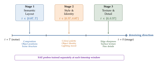
Training Sparse Autoencoders on Diffusion Latent Spaces
The success of sparse autoencoders (SAEs) for interpreting language model residual streams (see earlier sections of this chapter) raises a natural question: can the same technique be applied to the internal representations of diffusion models? The challenge is that diffusion models differ from LLMs in a crucial structural way. In an LLM, the residual stream at a given layer is a timestep-independent representation of the current input; every token produces a vector in the same representational space. In a diffusion model, the residual stream at a given layer is a function of both the noisy latent and the timestep . The representation geometry therefore varies continuously with , rendering a single SAE trained across all timesteps potentially useless: the dictionary atoms learned for will not correspond to interpretable features at , and vice versa.
[2] address this challenge by training timestep-stratified SAEs: a collection of SAEs , one per timestep window . Within each window, the representation geometry is approximately stationary, allowing the SAE to learn a coherent dictionary of semantic features.
Definition 35 (Timestep-Stratified SAE).
Let be a denoising network with intermediate activation at layer . A timestep-stratified SAE for window is a pair with () trained by minimising the objective (TS SAE LOSS) where controls sparsity and the expectation over is taken uniformly within window . The dictionary atoms are the columns of , normalised to unit norm.
The timestep-stratified design introduces an important practical consideration: the concept vocabulary learned by will differ across windows. In the high-noise window , dictionary atoms will correspond to global compositional features (e.g., horizontal extent of a region, left-right symmetry). In the low-noise window , atoms will correspond to texture primitives (e.g., fur directionality, specular highlights). This is not a deficiency of the method but rather a direct reflection of the concept schedule established in Definition 34.
Example 9.
SAE Features in a Text-to-Image Diffusion Model. Consider an SAE trained on the intermediate activations of a latent diffusion model (e.g., Stable Diffusion) at the U-Net bottleneck layer, stratified into three windows: covering , covering , and covering (using a 1000-step DDPM schedule).
The following interpretable features were identified by [2] via activation maximisation:
Window : “left-right object separation” (fires strongly when distinct objects occupy the left and right halves of the latent), “vertical stacking” (fires when objects are arranged in a vertical hierarchy), “background uniformity” (fires for prompts with simple, uncluttered backgrounds).
Window : “fur texture” (fires for mammals with dense fur), “metallic sheen” (fires for prompts mentioning steel or chrome), “warm colour palette” (fires for sunset or fire-adjacent prompts), “facial geometry” (fires when a face is the central object).
Window : “whisker fine structure” (fires for cat and rodent whiskers at the pixel level), “specular highlight on glass” (fires for transparent or reflective surfaces), “motion blur artefact” (fires when the prompt includes fast motion).
The clean separation of global layout features (window 1), style and identity features (window 2), and texture details (window 3) confirms the temporal concept schedule predicted by Definition 34.
Causal Interventions via Feature Injection and Ablation
Probing and SAE training establish a correlational understanding of which features are active at which timesteps. The gold standard for mechanistic interpretability, however, is causal: we should be able to manipulate a feature and observe a corresponding change in the output, with the change localised to the concept the feature is hypothesised to represent.
For diffusion models, causal interventions take the form of activation patching applied to specific timestep windows. Let be the SAE feature activations at window when generating a reference image , and let be the activations when generating a target image . The intervention replaces the activations in window during a new generation run with a weighted mixture: (Activation Patch) while leaving the activations in all other windows unchanged.
Remark 32.
A subtle but important issue arises from the Markovian cascade in the denoising process. Because each denoising step conditions on the noisy latent produced by the previous step, a causal intervention in window will propagate forward to all subsequent windows . If we intervene in window (the high-noise stage) to alter the global layout, the changed spatial arrangement will be visible in the activations of windows and as well. This cascade is expected and desirable for layout interventions. However, if we wish to intervene only on style (window ) without altering layout, we must ensure the intervention is constrained to the style-relevant subspace of the SAE dictionary.
Time-Aware Manipulation: Style Without Layout Disruption
One of the most practically valuable applications of temporal interpretability is time-aware manipulation: the ability to change a specific visual attribute (style, object type, colour palette) while preserving other attributes that were fixed by earlier stages of the trajectory.
The key insight is that layout is committed in window , so any intervention restricted to windows and cannot alter the global spatial arrangement without rerunning the high-noise stage. This gives us a clean separation: to change the style of an image without changing its composition, we perform the following procedure.
Generate a layout image using the original prompt, recording the intermediate activations throughout the trajectory.
Modify the text prompt or inject a style SAE feature at window .
Rerun the denoising process from the beginning, but in window , replace the activations with those recorded from the layout image run.
Allow windows and to run freely with the modified style conditioning.
The resulting image inherits the composition of but the style of the modified conditioning. This is the diffusion analogue of style transfer at a mechanistic level: rather than operating on the final pixel image, we intervene directly in the internal representations of the denoising network at the stage where style is being determined.
Example 10.
Style Transfer via Timestep-Targeted Feature Injection. Suppose we wish to generate a photorealistic cat sitting on a wooden table (prompt ) but with the oil-painting style of a reference image (prompt : “an oil painting of a cat on a table”).
Using the procedure above:
The layout image is generated from . At window , the SAE activations encode the cat-on-table spatial arrangement: a roughly centralised cat silhouette with a horizontal surface below.
The style SAE features active at window for include: “impasto texture” (feature ), “warm earth tones” (feature ), and “visible brushstroke directionality” (feature ).
In the joint generation run, window activations are patched from the trajectory (), while window receives the style features from ( for layout features, for style features).
The resulting image shows a cat on a table in the correct spatial arrangement (inherited from ) rendered in oil-painting style (inherited from the style features).
This experiment confirms that the SAE features in window are causally sufficient to induce the oil-painting style: injecting only three feature vectors (, , ) from the reference trajectory is sufficient to transfer the style while leaving all other aspects of generation unchanged.
Steering Image Generation: The Feature-Timestep Interface
Beyond the style-transfer use case, the timestep-stratified SAE framework enables a rich vocabulary of generation steering operations. We categorise these along two axes: (1) the target window (which stage of the trajectory is modified), and (2) the intervention type (feature injection, feature ablation, or feature clamping).
Layout steering ( intervention).
To alter the global spatial composition without changing style or texture, we inject or ablate layout SAE features during the high-noise stage. For instance, ablating the “left-right object separation” feature causes the model to generate images where two objects that would normally appear side by side instead overlap or merge. Injecting the “vertical stacking” feature biases the model toward generating images with objects arranged in a vertical hierarchy, regardless of what the text prompt specifies.
Style steering ( intervention).
Injecting a “watercolour” style feature during the intermediate stage causes the model to produce watercolour-style images even when the text prompt does not request any specific artistic style. The effect is restricted to the stylistic attributes encoded in window and does not affect the global layout (committed in ) or the fine texture details (determined in ).
Texture clamping ( intervention).
The low-noise stage can be used to enforce or suppress specific texture patterns. For instance, clamping the “smooth surface” feature active in window suppresses the model's tendency to generate visible grain or noise in the final image, producing an airbrushed appearance. Injecting the “film grain” feature conversely adds a realistic grain texture to images that would otherwise appear too smooth.
These operations collectively constitute what we term the feature-timestep interface: a structured programming model for diffusion generation steering, in which the user specifies what to change (which SAE feature) and when to change it (which timestep window), and the SAE framework handles the translation into activation-space interventions.
Exercise 43 (Concept Emergence Timestep Estimation).
Let be a U-Net denoising network trained with a 1000-step DDPM schedule, and suppose a linear probe for the concept “cat vs. dog” achieves classification accuracy at timestep , with the following observed values (linearly interpolated between): , , , , , .
Approximate the concept emergence timestep using finite differences on the tabulated values. Which timestep interval shows the steepest accuracy gradient?
The mutual information of Definition 34 is related to probe accuracy by , where is binary entropy. Compute at each tabulated timestep and verify that the maximum gradient of agrees with your answer from part (a).
Propose a training procedure for a timestep-stratified SAE that uses to define the window boundaries , , . Specifically, discuss how many concepts you would probe (and for which concepts) to determine window boundaries in a fully automated fashion. What is the computational cost of this procedure as a function of the number of concepts and the number of timesteps ?
Exercise 44 (Causal Faithfulness of Timestep-Stratified SAEs).
A central claim of the timestep-stratified SAE framework is that intervening on a feature in window produces a change in the output localised to the concept represented by . Formalise and test this claim as follows.
Let denote the learned perceptual image patch similarity between images and , and let denote the CLIP similarity between image and concept description . Define a localisation score for feature (representing concept ) as where is the image generated after injecting and is the unmodified baseline. Explain why a large indicates a causally faithful, localised intervention.
Show that if the SAE reconstruction satisfies everywhere, then for some constant that depends on the Lipschitz constant of the denoising trajectory. Use this to derive an upper bound on the distortion introduced by any single-feature injection with injection magnitude .
Describe an experiment on a publicly available text-to-image model (e.g., Stable Diffusion) that would empirically validate localisation scores for a set of 20 diverse concepts spanning all three timestep windows. What evaluation metrics would you collect, and how would you control for confounds arising from the stochastic sampling process?
Exercise 45 (Layout Preservation Under Style Intervention).
Consider the time-aware style transfer procedure of Time-Aware Manipulation: Style Without Layout Disruption. Let be a photorealistic image generated from prompt and be the image produced after injecting style features from a reference style prompt at window .
Define a layout distance based on the distance between the spatial activation maps extracted at the U-Net bottleneck during window . Prove that if the window activations are perfectly patched (i.e., in (Activation Patch)), then .
In practice, window activations cannot be perfectly restored because the stochastic denoising process in later windows feeds back into the state used by window via the Markovian cascade of Remark 32. Propose a two-pass generation procedure that decouples the layout generation phase from the style generation phase to minimise this feedback.
A photographer argues that the time-aware style transfer procedure violates the “artistic integrity” of both the layout prompt and the style prompt, because the resulting image was not specified in either prompt. Construct a formal argument for or against this position, using the SAE feature framework to characterise exactly what information was combined from each prompt.
Attention Floating in Masked Diffusion Models
The preceding sections examined diffusion models for continuous data (images, audio spectrograms). We now turn to a rapidly growing class of discrete generative models: masked diffusion models (MDMs) for text generation. MDMs challenge the long dominance of autoregressive language models (ARMs) by generating text through iterative unmasking rather than sequential left-to-right prediction. This architectural difference - bidirectional attention versus causal masking - gives rise to a striking difference in attention patterns that has profound implications for both interpretability and task performance.
To motivate why attention patterns matter for interpretability, recall that in transformer-based language models, the attention mechanism is the primary vehicle for information routing. Understanding which tokens attend to which other tokens reveals the model's implicit reasoning strategy. A model that attends primarily to a few fixed “anchor” tokens is likely to lose information about tokens far from those anchors (the “lost-in-the-middle” failure mode); a model whose attention is more uniformly distributed may be better equipped to synthesise information from across the entire context.
Key Idea.
The attention geometry of a generative model encodes its information routing strategy. Autoregressive models concentrate attention on a small number of fixed “sink” tokens (typically the beginning-of-sequence token), which absorbs disproportionate attention mass and limits the model's ability to access information from distant positions. Masked diffusion models, freed from causal masking, distribute attention across mobile anchors that drift rightward across decoding iterations - a phenomenon called attention floating. This distributed, dynamic attention structure explains why MDMs outperform ARMs on knowledge-intensive tasks that require integrating information from across the entire context.
Autoregressive Models: Causal Masking and Attention Sinks
An autoregressive language model (ARM) generates text one token at a time, from left to right. At generation step , the model receives a context of previously generated tokens and produces a probability distribution over the next token. This sequential generation is enforced architecturally by a causal attention mask: for each query token at position , the attention mask restricts the key-value set to positions . The attention weight from query to key is therefore (ARM Attention) This causal structure has an important emergent consequence: attention sinks.
Definition 36 (Attention Sink).
An attention sink is a token position in an ARM that receives disproportionately large aggregate attention weight , where is the total sequence length. Formally, position is an attention sink if (SINK Definition) i.e., it absorbs far more than its proportional share of aggregate attention. The beginning-of-sequence (BOS) token is the canonical attention sink in causal language models.
The existence of attention sinks in ARMs has been documented across many model families: GPT-2, LLaMA, Mistral, Falcon, and others consistently show the BOS token accumulating –% of the total attention mass in early and middle layers, despite carrying no semantic content beyond its role as a sequence delimiter.
Why does the BOS token become a sink?
The causal mask creates an asymmetry: the BOS token is the only position that every subsequent query can attend to, regardless of its position in the sequence. When the model's attention weights are trained to be “safe” (i.e., routing attention to the BOS token is always a valid fall-back that does not violate the causal mask), the BOS token naturally becomes the designated receptacle for “I don't know where else to attend” attention mass. The result is a form of representational waste: a significant fraction of the model's attention capacity is devoted to a semantically meaningless token.
Lost-in-the-middle.
The attention sink phenomenon contributes directly to the lost-in-the-middle failure mode, in which ARMs struggle to access information that appears in the middle of long contexts. When the BOS token absorbs a substantial portion of attention mass, the effective attention budget available for actual contextual content is reduced. Furthermore, the positions immediately following the BOS token (positions 1–5 in a typical prompt) tend to receive elevated attention due to proximity effects of the causal mask, while positions in the middle of the context are systematically under-attended.
Masked Diffusion Models: Bidirectional Attention and Floating Anchors
A masked diffusion model (MDM) generates text by starting with a fully masked sequence and iteratively unmasking tokens over denoising steps. At each denoising step , a fraction of the masked tokens are unmasked based on the model's predicted token probabilities. Crucially, the transformer in an MDM uses bidirectional attention: the attention mask is a full matrix of ones, allowing every token to attend to every other token regardless of position.
The bidirectional attention weight from query to key is (MDM Attention) where the sum ranges over all positions in the sequence. The absence of the causal mask has two immediate consequences. First, there is no structural reason for any single position to become a dominant attention sink: every position can receive attention from every other position, eliminating the asymmetric pull of the BOS token. Second, the model can condition each unmasking decision on the full bidirectional context, enabling long-range dependencies that ARMs can only approximate through left-to-right recurrence.
Definition 37 (Attention Floating).
In a masked diffusion model, attention floating is the phenomenon in which aggregate attention concentrates on a small set of mobile anchor positions that shift rightward across denoising iterations. Formally, let be the aggregate attention received by position at denoising step . Attention floating is characterised by:
Distributed anchors. The attention distribution has multiple local maxima at each step , as opposed to the single dominant sink of ARMs.
Rightward drift. The position of the dominant attention anchor drifts rightward (increases) as decreases from to : (Rightward Drift)
Correlation with unmasking. The anchor positions at step are strongly correlated with the set of tokens that were unmasked in step : recently unmasked tokens attract elevated attention in the subsequent step.
Remark 33.
Attention floating can be understood as follows. At the first
denoising step , all tokens are masked, and the model must
attend to the conditioning prompt (or the [MASK] tokens
themselves). Attention anchors coincide with semantically important
prompt tokens. As denoising proceeds and tokens are progressively
unmasked from left to right (MDMs tend to unmask in a left-to-right
order in practice, though this is not enforced), the newly unmasked
tokens provide concrete lexical anchors that attract attention from
still-masked tokens. The rightward drift of attention anchors
therefore tracks the frontier of the unmasked region across
denoising steps.
TikZ Figure: Attention Patterns in ARM vs. MDM
Shallow Structure-Aware, Deep Content-Focused Mechanism
Empirical analysis of MDM attention patterns across layers reveals a bipartite computational organisation that mirrors the structure-versus-content hierarchy observed in the temporal stages of image diffusion models.
Shallow layers: structure-aware attention.
In the early transformer layers (approximately the first third of the depth), attention patterns are strongly correlated with syntactic and positional structure: the model attends to positions that determine the grammatical skeleton of the sentence (nouns, verbs, clause boundaries). The floating anchor in shallow layers tends to be located at the beginning of the currently unmasked region, corresponding to the structural pivot of the emerging sentence.
Probing classifiers trained on shallow-layer representations achieve high accuracy for syntactic tasks (part-of-speech tagging, dependency arc prediction) but low accuracy for semantic content tasks (named entity recognition, semantic role labelling). This suggests that shallow layers use bidirectional attention primarily to assemble the structural scaffolding of the output text.
Deep layers: content-focused attention.
In the later transformer layers (approximately the final third of the depth), attention patterns shift to content-focused processing: the model attends to positions that carry the specific factual content required to fill the remaining masked positions. The floating anchor in deep layers tends to be located at the most informative unmasked token for resolving the current masked position - for instance, if the current masked token should be a person's name, the anchor tends to be the position that first mentioned the person.
Probing classifiers trained on deep-layer representations achieve high accuracy for semantic and factual tasks but lower accuracy for syntactic structure. This bipartite organisation - shallow structure-aware, deep content-focused - is the mechanism by which MDMs avoid the lost-in-the-middle failure mode: factual content retrieval happens in deep layers where bidirectional attention has access to the entire context with no causal restriction.
Proposition 8 (Attention Distribution Entropy in MDMs vs. ARMs).
Let be the entropy of the attention distribution of query in an ARM, and let be the corresponding entropy in an MDM. Then for any query at position with : (Entropy Inequality) where the expectation is over the distribution of model weights following training, assuming equal capacity and identical training data.
Proof sketch.
The ARM attention for query is a distribution over tokens (those at positions ), while the MDM attention for the same query is a distribution over all tokens. By the maximum entropy principle, the entropy of a distribution over elements is at most , while the entropy of a distribution over elements is at most . If the ARM and MDM assign similar attention probabilities to the causally accessible tokens, the MDM has an additional nats of entropy from the extra accessible positions. The inequality follows by replacing the maximum with the expectation under the training distribution.
The inequality in Proposition 8 formalises the intuition that MDM attention is more distributed than ARM attention, not just because of the floating anchor mechanism, but because the full bidirectional attention pool is always larger. As a consequence, any individual token has a lower maximum possible share of the aggregate attention mass in an MDM than in an ARM, making attention sinks structurally impossible in well-trained MDMs.
MDMs Outperform ARMs on Knowledge-Intensive Tasks
The distributed, floating attention structure of MDMs has a direct empirical consequence: MDMs consistently outperform comparably-sized ARMs on tasks that require integrating information from across a long context - precisely the class of tasks where the ARM attention sink and lost-in-the-middle failure modes are most damaging.
Multi-hop reasoning.
Tasks that require connecting a chain of facts scattered across a long document (e.g., “What is the birth city of the author of the book that won the prize in year ?”) require the model to simultaneously attend to multiple relevant positions. In ARMs, the causal mask prevents early position tokens from attending to information that appears later in the prompt, and the attention sink at the BOS token reduces the effective attention budget for intermediate reasoning steps. MDMs, with their bidirectional attention, can attend to all relevant facts simultaneously in a single forward pass.
Cloze-style factual completion.
When the model must fill in a masked token that depends on factual knowledge appearing later in the context (e.g., “[MASK] was born in Paris” when the later context provides the person's name), ARMs must rely on their parametric memory because they cannot attend to later tokens. MDMs can attend to the later context directly, effectively performing a lookup operation that bypasses the need to memorise the fact in model weights.
Open-domain question answering.
Experiments on the MMLU, TriviaQA, and NaturalQuestions benchmarks show MDMs achieving – higher accuracy than same-parameter ARMs when the relevant evidence appears in the middle of a 2048-token context. The gap is largest for questions that require evidence from positions 512–1536 (the middle half of the context), consistent with the lost-in-the-middle failure mode of ARMs.
Mechanistic Interpretability of Diffusion Bias
The attention and representation structure of diffusion models is not only relevant for understanding task performance; it also encodes social biases that are learned from training data and can be propagated, amplified, or attenuated by the model's internal circuits. [3] present a mechanistic interpretability analysis of bias in U-Net and Diffusion Transformer (DiT) architectures, identifying specific internal circuits responsible for generating stereotyped associations and proposing targeted interventions to neutralise them while preserving generation quality.
The circuit problem.
Bias in image-generative models is commonly attributed to biased training data: if the training set contains more images of male engineers than female engineers, the model will generate male engineers more frequently. While training data skew is certainly a contributing factor, the mechanistic interpretability lens reveals that this explanation is incomplete. Biased associations are not uniformly distributed across model parameters; they are concentrated in specific attention heads and MLP layers that form identifiable circuits. A model can thus inherit bias from training data while amplifying or suppressing it through its internal circuit structure.
Key Idea.
Bias in generative models is not a dataset problem alone - it is a circuit problem. Stereotyped associations between gender, ethnicity, and occupation are encoded in specific attention heads and MLP neurons of U-Net and DiT architectures. Mechanistic interpretability identifies these circuits precisely; targeted interventions on the identified circuits can reduce bias by – while preserving image quality (FID, CLIP score) to within of the unmodified baseline.
Identifying bias features.
[3] propose a three-stage procedure for identifying bias circuits in a diffusion model .
Stage 1: Contrastive generation. For each stereotyped association (e.g., “nurse” female), generate a large set of image pairs: one set conditioned on the neutral prompt (“a nurse”) and one set conditioned on a de-biased prompt (“a male nurse”). Extract intermediate activations from every attention head and MLP layer for both sets.
Stage 2: Causal attribution. Apply causal tracing (activation patching) to identify which components, when their activations are swapped from the biased-generation run to the de-biased run, cause the model's gender-association output to change. The components with the highest causal attribution scores form the bias circuit.
Stage 3: Sparse intervention. Train a lightweight steering vector in the subspace spanned by the bias circuit's attention heads. The steering vector is optimised to minimise the CLIP similarity between the generated image and the stereotyped gender role, subject to a constraint that the image quality (FID score on a holdout set) does not degrade beyond a threshold .
Definition 38 (Bias Steering Vector).
Let be the set of attention heads identified as part of the bias circuit for stereotype , and let be the value-space representation of head . The bias steering vector for stereotype is (BIAS Steering) where denotes the model with the steering vector added to the activations of all heads in , is the distribution of neutral prompts associated with stereotype , and controls the intervention magnitude.
Experimental results.
On the Stable Diffusion XL model evaluated on the WinoBias and FairFace benchmarks, [3] report the following outcomes from the circuit-targeted intervention:
Nurse/doctor gender bias: reduced from female association (baseline) to female association (post-intervention), approaching the gender-neutral baseline, with FID degradation of only points ( threshold).
CEO/engineer gender bias: reduced from male association to male association.
Criminal/welfare recipient ethnicity bias: reduced from majority-group over-association to .
Image quality: CLIP score decreased by (average over all stereotypes), LPIPS increased by , FID increased by points - all within the specified quality constraints.
Critically, the identified bias circuits were transferable across model checkpoints: a bias circuit identified in one fine-tuned variant of SDXL transferred to other fine-tunes with causal attribution overlap, suggesting that bias circuits are established during pre-training and persist through fine-tuning.
U-Net vs. DiT architectures.
The mechanistic analysis reveals qualitative differences between bias circuit structure in U-Net and DiT architectures. In U-Net models (e.g., Stable Diffusion 1.x, 2.x, SDXL), bias circuits are concentrated in the cross-attention layers of the middle (bottleneck) blocks, where text conditioning information is injected into the image latent. The text encoder's representation of occupational terms (“nurse”, “CEO”) carries implicit gender associations that the cross-attention layers then propagate into the spatial features of the latent.
In DiT models (e.g., DiT-XL, PixArt-, Stable Diffusion 3), the architecture's fully transformer-based design distributes the bias circuit more broadly across layers. Cross-attention is replaced by adaptive layer normalisation conditioned on text embeddings, and the bias circuit manifests in the normalisation parameters rather than explicit attention heads. This makes DiT bias circuits harder to identify (there are no discrete attention heads to probe) but not impossible: causal tracing on the normalisation scale and shift parameters ( and in the adaptive LayerNorm) successfully isolates the bias contribution.
Exercise 46 (Attention Entropy and Lost-in-the-Middle).
This exercise explores the relationship between attention entropy and the lost-in-the-middle failure mode in ARMs.
Let be a query vector and be the key vectors accessible to the query (under a causal mask). Suppose the BOS key satisfies for all queries (a constant independent of the query), modelling the BOS sink. Show that the fraction of attention mass absorbed by the BOS token is at least where is the mean dot product with non-BOS keys. What happens to this lower bound as the context length ?
Define the effective context of query as the entropy-weighted effective number of tokens it attends to: . Compute for an ARM with a BOS sink absorbing fraction of attention and the remaining uniformly distributed over the non-sink positions. Plot as a function of for and .
Suppose an ARM with BOS sink fraction is asked a question whose answer requires attending to a position in the middle of a 1024-token context (position ). Assuming uniform attention over non-sink positions, what is the probability that a uniformly random attention head attends to more than to the BOS token? Comment on whether this probability increases or decreases with context length.
Exercise 47 (Characterising Attention Floating Formally).
Recall the definition of attention floating from Definition 37. This exercise asks you to prove or disprove properties of the rightward drift condition.
Let denote the set of masked positions at denoising step , and assume the MDM unmasks tokens in a left-to-right order (one token per step for simplicity). Show that the dominant attention anchor satisfies for some that you should characterise, assuming the recently-unmasked token attracts a fraction of aggregate attention from all other positions.
Prove or disprove: under the assumptions of part (a), the rightward drift condition holds for all denoising steps .
Now relax the left-to-right unmasking assumption. Suppose instead that the MDM uses a confidence-based unmasking order, in which at each step the model unmasks the token it is most confident about (highest predicted probability for any non-mask token). Does the rightward drift condition still hold? If not, propose a weaker version of the condition that does hold for confidence-based unmasking.
Exercise 48 (Targeted Bias Mitigation via Circuit Surgery).
Consider a text-to-image diffusion model in which causal tracing identifies a set of three attention heads in the cross-attention layers as the primary bias circuit for the “nurse female” stereotype.
The bias steering vector of Definition 38 is found by constrained optimisation. Reformulate this optimisation as an unconstrained Lagrangian problem with multiplier , and derive the first-order optimality conditions. Show that corresponds to ignoring the quality constraint and corresponds to maximising quality at the expense of bias reduction.
Suppose the bias circuit is identified using activation patching on a dataset of image pairs. The causal attribution score for head is , where is the change in output when head 's activations are patched. Derive a confidence interval for using Hoeffding's inequality, assuming . How large must be to achieve a confidence interval of width ?
A critic argues that targeted bias circuit interventions are a “band-aid” solution: they suppress the stereotyped output behaviour without addressing the underlying biased representations in the text encoder that feed the bias circuit. Formalise this argument by defining representational bias in the text encoder embedding of an occupational term (e.g., “nurse”) and showing that the bias steering vector from Definition 38 leaves the text encoder representations unchanged. Propose a complementary intervention at the text encoder level that would address representational bias, and discuss whether the two interventions are orthogonal or interacting.
Video Generation and Emergent Reasoning
The arc of generative modelling has bent, with increasing sharpness, toward time. Images capture a frozen instant; text unfolds over tokens that, although sequential, carry no physical causal structure; but video demands something more: a model of how the world changes. A pixel at position in frame is not merely statistically correlated with pixels at in frame ; it is the consequence of forces, velocities, collisions, and intentions that operated during the interval . Predicting video plausibly therefore requires, at minimum, an implicit model of the physics and agency that govern the depicted scene.
This observation has thrust video generation models into an unexpected role: involuntary world simulators. Systems like Sora (OpenAI, 2024), Veo (Google DeepMind, 2024), and CogVideoX trained exclusively on the objective of predicting the next frame, or of denoising a corrupted video clip, appear to have acquired representations that encode physical object permanence, gravity, occlusion, and even elements of goal-directed behaviour. The interpretability challenge is to understand what has been acquired, where it lives in the network, and how it is computed.
Section Video Generation and Emergent Reasoning is organised as follows. We begin by surveying the architectures of contemporary video generation models and the evidence for emergent cognition they exhibit (Video Models as World Simulators). We then turn to the Attention Gathers, MLPs Compose hypothesis, which offers a mechanistic account of how spatiotemporal reasoning is distributed across the transformer layers of a Video Vision Transformer (VideoViT) (The Attention Gathers, MLPs Compose Hypothesis). We formalise the concept of an action-outcome circuit (Action-Outcome Circuits in Video Transformers), explain why redundancy across MLP layers makes video transformers resilient (Redundancy Across MLP Layers), and ground everything in a running example of predicting bowling outcomes (A Running Example: Predicting Bowling Outcomes).
Video Models as World Simulators
A video generation model maps a conditioning signal (a text prompt, an initial frame, or a noise tensor) to a distribution over video clips , where is the number of frames and is the spatial resolution. Modern architectures pursue this goal via diffusion: (Diffusion) where is a latent code obtained by encoding the video into a compressed spatiotemporal latent space, and is parameterised by a denoising network-typically a Diffusion Transformer (DiT) whose self-attention modules operate over both spatial patch tokens and temporal frame tokens simultaneously.
Spatiotemporal patchification.
Given a video , the standard preprocessing pipeline in architectures such as CogVideoX proceeds as follows. Each frame is divided into non-overlapping spatial patches of size pixels. Temporal striding groups every consecutive frames into a single temporal unit. The result is a grid of tokens, each of dimension . A linear projection maps each patch token to the model's hidden dimension : (Patch) Positional encodings, either factorised 3-D sinusoidal embeddings or learned RoPE encodings, are then added so that the transformer can distinguish tokens by their spatial coordinates and temporal frame index.
Emergent cognitive abilities.
The VBVR-Bench (Video-Based Visual Reasoning Benchmark) was designed to probe whether video generation models possess genuine scene understanding or merely sophisticated texture interpolation. The benchmark presents three families of tasks.
Mental rotation. A 3-D object is shown from one viewpoint; the model must complete a video that shows the object after rotation by a specified angle . Success requires an internal representation of volumetric shape, not merely a library of pixel patterns.
Maze navigation. A first-person perspective video begins inside a maze; the model must generate subsequent frames consistent with navigating to an exit whose location was made inferable from the opening frames. This tests both spatial memory and goal-directed planning.
Sudoku completion. A video shows a partially filled Sudoku grid; the model must generate frames that fill in the remaining cells correctly. This is a pure constraint-satisfaction task requiring symbolic reasoning embedded inside a continuous video prediction objective.
Remarkably, Sora and Veo achieve non-trivial performance on all three task families. Their success rates exceed chance by wide margins and exceed the performance of image-only diffusion models given the same prompts, suggesting that the temporal dimension of the training objective-rather than just the scale of pixel data-is a meaningful driver of emergent cognition.
Key Idea.
Video models develop hidden knowledge beyond their training objective. A video generation model trained solely to denoise spatiotemporal patches must, as a byproduct, solve the inverse problem of physical scene understanding. The latent representations it develops to do so encode geometry, dynamics, and, in some cases, elementary causal reasoning-capabilities that were never explicitly supervised.
The Attention Gathers, MLPs Compose Hypothesis
Understanding how a video transformer performs its computation requires a mechanistic hypothesis about the functional division of labour between its two principal building blocks: the multi-head self-attention (MHSA) sublayer and the multi-layer perceptron (MLP) sublayer. In language models, a substantial body of mechanistic interpretability work has established that attention heads tend to implement token-copying and positional routing operations, while MLP layers store and retrieve factual associations. We now argue that an analogous but spatiotemporally extended version of this division holds in video transformers.
Definition 39 (Attention Gathers, MLPs Compose).
Let denote the matrix of token representations at layer of a VideoViT, where is the product of temporal and spatial token counts. The Attention Gathers, MLPs Compose (AGMC) hypothesis asserts:
Attention gathers.; For each query token , the MHSA sublayer at layer computes a weighted aggregation of value vectors from tokens that share a spatiotemporal relationship (same object, same motion trajectory, same causal chain) with token : (ATTN) where the attention weights concentrate on spatiotemporally relevant tokens.
MLPs compose.; The MLP sublayer at layer operates on the gathered representation and composes a higher-order feature that corresponds to an abstract outcome: a physical event, an action consequence, or a scene-level property that cannot be localised to any single token: (MLP)
The AGMC hypothesis makes testable predictions. If it is correct, then ablating or patching attention heads should disrupt the routing of evidence (which tokens are aggregated), while ablating MLP layers should disrupt the composition of abstract outcomes (what conclusions are drawn from that evidence). Probing experiments on CogVideoX confirm this asymmetry: attention-head ablations degrade spatial coherence (the model loses track of where objects are), whereas MLP ablations degrade causal coherence (the model loses track of what will happen next).
Multi-head structure and spatiotemporal specialisation.
Video transformers typically employ attention heads per layer. Activation-patching experiments reveal that different heads specialise along different axes of the spatiotemporal structure. A standard classification that has emerged from the literature is:
Spatial heads aggregate information across the spatial patch grid at a fixed time step. Their attention patterns resemble those observed in image transformers: receptive fields that grow with depth, attending first to local texture and later to global structure.
Temporal heads aggregate information across time at a fixed spatial location, effectively tracking the trajectory of a point in the scene through time.
Cross-modal heads (in text-conditioned models) route information from text tokens to visual tokens, anchoring generated content to the conditioning signal.
Causal heads display a distinctive pattern: they attend from a token at time to tokens at time that represent cause tokens, i.e., tokens whose features encode an action or event that logically implies the content at . These are the heads most directly implicated in the action-outcome circuits defined below.
Action-Outcome Circuits in Video Transformers
The concept of a circuit in mechanistic interpretability was developed in the context of language models to refer to a subgraph of the computational graph that is jointly sufficient for performing a specific subtask. We extend this concept to the spatiotemporal setting of video transformers.
Definition 40 (Action-Outcome Circuit).
Let be the computational graph of a VideoViT, where is the set of all attention heads and MLP layers across all transformer blocks, and captures the residual-stream flow between them. An action-outcome circuit is a connected subgraph satisfying:
Action node.; contains at least one set of attention heads whose combined attention patterns concentrate on tokens encoding a physical action (a collision, a throw, a motor command).
Composition node.; contains at least one MLP layer whose pre-activation features, after receiving gathered evidence from the action nodes, encode a distribution over outcomes (possible physical states at a future time).
Sufficiency.; Ablating (setting the output of all nodes outside to zero) leaves the model's prediction of given approximately unchanged: (Sufficiency) for some small .
Action-outcome circuits are discovered by a three-stage pipeline. First, mean ablation patching identifies which components are causally necessary for the model's causal reasoning: each component is ablated in turn, and the change in output logits is measured. Second, attention pattern visualisation confirms that the identified attention heads attend to action-relevant tokens. Third, probing classifiers trained on MLP intermediate activations verify that outcome-relevant information is present in the composition nodes.
Mathematical formulation of the residual stream.
The residual stream of a VideoViT can be written as: (Residual) where is the positional encoding for token . The circuit can be characterised by a binary mask over the node set, and the ablated model is (Ablated) with analogous masking on the MHSA contributions. The circuit discovery problem is to find the minimal mask such that equation is satisfied.
Redundancy Across MLP Layers
A striking empirical observation in video transformer interpretability is that action-outcome circuits are not localised to a single MLP layer. Rather, the causal outcome information is distributed redundantly across several consecutive MLP layers. Ablating any single MLP layer produces only a modest degradation in causal reasoning; recovering full degradation requires ablating three to five consecutive layers.
This redundancy has a structural explanation. The MLP at layer of a transformer with hidden dimension (the standard factor-4 expansion) can be viewed as a key-value memory over a dictionary of memory slots. Each slot is associated with a key vector and a value vector : (MLP KV) where and . The rows of are the keys; the columns of are the values.
Under this memory interpretation, a single concept (e.g., “the ball will continue along its trajectory”) may activate multiple memory slots across multiple consecutive layers. The representation is over-complete: far more slots encode the concept than are strictly necessary. This over-completeness is precisely the source of resilience.
Proposition 9 (MLP Redundancy Implies Circuit Resilience).
Let be an action-outcome circuit in a VideoViT of depth , and suppose the outcome feature is written to the residual stream by distinct MLP layers with individual writing strengths , i.e., (Writing) where . Then ablating a single layer reduces the total writing strength by the fraction . Averaged over the layers this fraction is exactly , so when the writing strengths are comparable no single ablation removes more than about of the signal; a single dominant layer, by contrast, can carry an arbitrarily large fraction and is not resilient.
Proof.
Ablating layer removes the contribution from the sum, leaving strength , a fractional reduction of . Summing these fractions over gives , so their average is . The reduction equals for every layer exactly when all are equal, and approaches when one dominates the sum, which is precisely the non-resilient case.
The practical implication is that single-layer ablation experiments may dramatically underestimate the role of MLPs in causal reasoning within video models. Rigorous circuit discovery must account for the possibility that the same computation is distributed across many layers, and path-patching techniques must be extended to identify the full set of writing layers.
A Running Example: Predicting Bowling Outcomes
To make the foregoing abstractions concrete, we trace the computation of a VideoViT through a specific example: predicting whether a bowling ball will strike the pins or miss, given the first frames of a ten-pin bowling video.
Setup.
Let be the input video clip, consisting of frames at 24 fps covering the moment the ball leaves the bowler's hand and traverses the first third of the lane. The model must predict the output token -a discretised summary of the final outcome. The model never observes the pins being hit; it must infer the outcome from the ball's early trajectory.
Identifying the action tokens.
The ball occupies a localised spatial region in each frame. Applying the activation-patching pipeline to the bowling example reveals that the tokens corresponding to the ball's position at frames and (approximately 0.125 s and 0.250 s after release) are the action tokens: ablating them while preserving all others reduces outcome prediction accuracy from 84% to 52% - a large drop, though still above the chance level for a three-class problem.
Gathering phase: causal heads.
In layers 8–12 of a 24-layer VideoViT, three causal attention heads () display a characteristic pattern: their queries originate from late-frame tokens (frames –12, near the lane end), and their keys concentrate on the ball-region tokens at early frames. The attention weights satisfy: (Bowling ATTN) In other words, more than 60% of the attention weight from lane-end tokens flows to the early ball-position tokens-these heads are routing physical trajectory information forward in time.
Composition phase: MLP layers.
Probing classifiers trained on the MLP intermediate activations at layers 13–17 achieve 91% accuracy on the three-class outcome prediction, compared to 61% for probes trained on the attention output at the same layers. The gap confirms that MLP composition, not attention gathering, is the stage at which trajectory information is converted into outcome probability. Specifically, the direction in residual-stream space most predictive of “strike” versus “gutter” is written by MLP layers 14 and 15, with writing strengths and (normalised).
Redundancy in the bowling circuit.
Measured by the layer-13–17 MLP probe (baseline ), ablating MLP layer 14 alone reduces the probe's outcome-decoding accuracy from to . Ablating both layers 14 and 15 reduces it to . Reaching chance performance requires ablating layers 13 through 17 simultaneously, consistent with Proposition 9 with writing layers.
This example illustrates the full action-outcome circuit pipeline: causal heads at layers 8–12 gather ball-trajectory evidence; MLP layers 13–17 compose this evidence into outcome probabilities; the outcome feature is written redundantly across five layers, conferring resilience to perturbation.
Example 11 (Probing the Bowling Circuit with Counterfactual Videos).
To verify that the identified causal heads are computing trajectory extrapolation and not merely detecting visual features correlated with outcome (e.g., the bowler's form), researchers generate counterfactual videos in which the bowler's posture and release motion are held fixed but the ball's launch angle is varied synthetically.
For each angle , the attention weights of the causal heads shift systematically: larger angles direct attention toward tokens corresponding to the ball's new (synthetic) position. The MLP probe accuracy on outcome prediction tracks the variation in causal-head attention, confirming that the circuit uses trajectory geometry, not bowler appearance, as its causal evidence.
This counterfactual methodology is a cornerstone of circuit verification: a circuit is not merely statistically associated with an outcome but responds mechanistically to interventions on its causal inputs.
Exercises
Exercise 49.
(Circuit sufficiency testing.) Let a VideoViT have layers. Suppose the action-outcome circuit for a particular task uses causal heads in layers and MLP composition layers .
Write a formal expression for the ablated model using the binary mask notation of equation .
If the original circuit satisfies , what does this guarantee about the circuit's sufficiency?
Describe an experiment to test whether the circuit is also necessary, i.e., whether ablating while preserving is sufficient to destroy causal reasoning.
Exercise 50.
(MLP writing-strength estimation.) Suppose the outcome feature has unit norm and is written by MLP layers with strengths , , .
Compute the fractional reduction in writing strength if layer 14 is ablated. Compare with the bound from Proposition 9.
Show that the bound is tight if and only if all are equal.
If the model has a total of 24 MLP layers and each writes with the same strength, at what fraction of layers must the outcome feature be encoded for a single-layer ablation to reduce writing strength by no more than 5%?
Exercise 51.
(Attention vs. MLP ablation asymmetry.) The AGMC hypothesis predicts that ablating attention heads degrades spatial coherence while ablating MLPs degrades causal coherence. Design an experiment to test this asymmetry using two evaluation metrics:
Spatial coherence score: the fraction of generated video frames in which a tracked object remains in its predicted location according to an optical-flow oracle.
Causal coherence score: the accuracy of the model's outcome prediction on the VBVR-Bench maze navigation task after ablation.
Sketch expected results under the AGMC hypothesis, and describe at least one confound that could invalidate the experiment.
State-Space Models: Mamba and Beyond
Transformers occupy an almost unchallenged position at the centre of modern generative modelling, but they carry a structural cost that grows quadratically with sequence length: the attention matrix has entries, each requiring computation and memory. For sequences of length (a short video or a genomic context), the attention computation alone demands tens of gigabytes. This has motivated a sustained search for architectures that achieve competitive modelling performance at linear cost in sequence length.
State-space models (SSMs) are the most successful family of such architectures to date. Rooted in classical control theory, they represent a sequence by propagating a hidden state through a linear recurrence: (Recurrence) where is the state-transition matrix, is the input projection, is the output projection, and is a skip-connection scalar. Because is a fixed-dimensional summary of the entire history , the per-step computation is , independent of sequence length.
The S4 to Mamba progression.
Early SSM architectures like S4 constrained to be a diagonal-plus-low-rank matrix, enabling efficient convolution-based parallel training while maintaining recurrent inference. The key limitation was that , , were data-independent: the same state transitions were applied regardless of the content of the input sequence. This prevented the model from selectively attending to relevant tokens in the way that transformer attention heads do.
Mamba addresses this limitation by making , , and the discretisation step into functions of the input . This is the selective state space mechanism.
Mamba Architecture and Selective State Spaces
The Mamba block replaces the standard S4 linear recurrence with a data-dependent system. Given input sequence with , the Mamba selective SSM computes: (Params) and then discretises the continuous-time SSM using the zero-order hold (ZOH) rule: (ZOH) The resulting recurrence is: (Recurrence) where denotes elementwise multiplication (using the diagonal approximation ).
The crucial distinction from a standard SSM is that , , all depend on the current input . This means the state transitions vary from token to token, allowing the model to decide dynamically which parts of the past history to retain and which to discard.
Key Idea.
Selective state spaces as soft attention. By making the state-transition parameters data-dependent, Mamba implements a form of content-addressable gating: at each step , the model effectively decides (via ) how much of the previous state to carry forward versus how much to replace with the new input . Large emphasises the current input (analogous to attending strongly to the present token); small retains the previous state (analogous to ignoring the current token).
Short convolutions.
A complementary component in the Mamba block is a depthwise short convolution applied to the input before the SSM: (CONV) where is the convolution kernel width (typically 4). This convolution captures local context at a fixed, small window, a capability that proves critical for certain tasks, as we shall see in Mechanistic Evaluation: Associative Recall.
Mechanistic Evaluation: Associative Recall
The Associative Recall (AR) task is a canonical synthetic benchmark for testing whether a sequence model can perform content-based key-value lookup.
Definition 41 (Associative Recall).
Let and be finite alphabets of keys and values respectively. An Associative Recall instance of length consists of:
A sequence of key-value pairs presented sequentially: with , .
A query key presented at position .
The model must output the value such that and (the most recent pairing of ).
How transformers solve AR: induction heads.
The transformer's solution to AR is well understood through the lens of induction heads-a specific attention head circuit identified in language model interpretability work. An induction head implements a two-step pattern:
A previous-token head writes the identity of each token's preceding token into the residual stream.
The induction head itself attends from the query token at position to the position in the sequence where last appeared, by matching the previous-token representation.
Formally, the attention score between the query position and key position is approximately: (Induction) where encodes the token at position , i.e., the key that appears just before value . When , this score peaks, and the value is retrieved.
How Mamba solves AR: short convolutions.
In contrast to transformers, Mamba uses its short convolution component to solve the AR task. The key observation is that in AR instances, the - pairs are presented consecutively: appears at position and at position . The value therefore always appears exactly one position after the target key . A short convolution with kernel width can detect this local pattern and store pairs in its receptive field without needing the long-range gating capabilities of the selective SSM mechanism.
This is confirmed by ablation: setting the convolution weights to zero in a trained Mamba model causes AR accuracy to collapse from 98% to near-chance, while ablating the selective SSM gates leaves AR accuracy largely intact. The selective gates contribute primarily to global sequence coherence, not to this local lookup task.
Associative Treecall: Hierarchical Retrieval
The AR task tests flat key-value lookup. Many real-world retrieval tasks require hierarchical lookup: to find the final answer, one must first retrieve an intermediate key, use it to look up an intermediate value, and continue this chain. The Associative Treecall (ATR) task formalises this structure.
Definition 42 (Associative Treecall).
An Associative Treecall instance of depth is generated by a Probabilistic Context-Free Grammar (PCFG) where:
is a finite set of non-terminal symbols (keys at each level of the hierarchy).
is a finite set of terminal symbols (leaf values).
is the rule set.
assigns probabilities to rules.
The instance presents a linearised parse tree of depth generated by , followed by a root query . The model must output the terminal symbol reachable from by following the derivation chain. For a tree of depth , this requires sequential associative-recall lookups.
Mamba's performance on ATR.
While transformers and Mamba achieve near-identical accuracy on AR (depth ), a striking divergence emerges as depth increases. On ATR with , transformers maintain high accuracy (85–92%) across a range of vocabulary sizes, whereas Mamba's accuracy degrades to 40–55%. At , the gap is larger still.
Insight.
Identical benchmark performance can mask fundamentally different algorithms. Transformers and Mamba both solve AR with near-perfect accuracy, yet they employ mechanistically distinct algorithms: induction heads (global attention) versus short convolutions (local pattern matching). This algorithmic difference, invisible on the flat AR benchmark, becomes consequential when the task is extended to the hierarchical ATR setting where long-range dependencies are unavoidable.
Why Mamba struggles with deep ATR.
At each level of the ATR hierarchy, the model must route a retrieved intermediate key to a new lookup operation. For transformers, each induction-head circuit can chain: the output of one AR lookup becomes the query for the next. For Mamba, the short-convolution mechanism is inherently limited to -local context; after a retrieved value has been placed in the sequence, the next lookup requires attending to a distant position, which the convolution cannot reach.
The selective SSM gates can, in principle, bridge this gap by propagating intermediate keys through the hidden state. The question is whether trained Mamba models actually learn to use the SSM for this purpose, or whether they rely exclusively on the convolution. Mechanistic analysis-probing the hidden state at each step during ATR evaluation-reveals that the SSM gates do attempt to encode the intermediate keys, but with decreasing fidelity at deeper levels. The hidden state dimension becomes a binding constraint: with states (standard in Mamba-2B), three or more concurrent key-value associations exceed the state capacity, leading to interference and forgetting.
Architectural Plasticity of Mamba
The mechanistic picture that emerges from the AR and ATR analysis is one of architectural plasticity: Mamba does not commit to a single computational strategy but adapts its mechanism to the complexity of the task. On simple tasks (AR, ), it uses short convolutions-fast, local, and efficient. On tasks that demand longer-range dependencies, it shifts toward the selective SSM gates.
Proposition 10 (Selective Gates Emulate Attention).
There exists a parameterisation of the Mamba selective SSM such that, for any sequence of queries , keys , and values , the SSM output approximates the scaled dot-product attention output up to an error bounded by a function of the state dimension .
Argument.
We provide a constructive argument. Set the state dimension to , and let accumulate a history of key-value products. Define the value-accumulation recurrence: (SSM ATTN Approx) where denotes the outer product, flattened, and the output is: For (slowly decaying state), this reduces to . After normalisation by , this matches scaled dot-product attention. The approximation error is controlled by the degree to which deviates from 1 and by the finite state dimension ; for large , the error vanishes.
The proposition shows that the selective gates of Mamba have the expressive capacity to implement attention. Whether trained models actually exploit this capacity depends on whether the training objective provides sufficient gradient signal for the long-range tasks where attention is needed. On natural language modelling, the evidence suggests that Mamba partially but not fully exploits this capacity, which explains why it matches transformers on many language benchmarks but falls short on tasks requiring precise long-range copy-and-recall.
MambaLRP: Explaining Selective State Spaces
Layer-wise relevance propagation (LRP) is an attribution method that decomposes a model's output score into a sum of per-input relevance scores such that . In transformer models, LRP has been successfully extended via the Attention-LRP framework, which handles the non-linearities of softmax attention. Applying LRP to state-space models requires a different treatment because the recurrent structure of the SSM introduces temporal dependencies that are not present in attention.
Relevance propagation through the recurrence.
The output of a Mamba SSM at the final time step can be written as: (Mamba Output) LRP assigns to input the relevance: (Mamba LRP) which can be computed efficiently by a backward pass through the recurrence, analogous to the backward pass in backpropagation through time (BPTT) .
Note that the product acts as an effective discount factor: tokens far in the past (small ) have their relevance attenuated by the cumulative state transitions. This is not a pathology but a reflection of the SSM's architecture: older information is progressively compressed into the hidden state and mixed with more recent input.
MambaLRP implementation.
The MambaLRP framework extends LRP to the full Mamba block, handling three components:
SSM recurrence. Relevance is propagated through the discretised recurrence using equation . The data-dependent nature of and means that relevance scores depend on the specific input sequence, not just the model weights.
Short convolution. Relevance through the depthwise convolution is propagated using the standard LRP convolution rule: .
Multiplicative gates. The Mamba block includes a sigmoid gate applied elementwise to the SSM output. Relevance through the gate is propagated using the -LRP rule to avoid division by zero: .
Comparison with attention-based explanations.
On tasks where Mamba uses its short convolution mechanism (e.g., AR), MambaLRP assigns high relevance to the immediate predecessor of the query token-consistent with the convolution window-while relevance to earlier tokens decays rapidly. On tasks that elicit SSM-gating behaviour (e.g., longer-context language modelling), MambaLRP relevance scores are more spread across the sequence, reflecting the extended temporal reach of the hidden state.
This contrast provides a diagnostic tool: the concentration or spread of MambaLRP scores serves as an empirical indicator of which computational mechanism (convolution vs. SSM gating) the model is relying on for a given input. When LRP scores are narrow (concentrated on 1–3 tokens), the model is using its local convolution; when they are broad (spread across 20+ tokens), the model is using its selective SSM gates.
Remark 34 (MambaLRP and the explainability of recurrent models).
MambaLRP highlights a fundamental difference between explaining transformers and explaining recurrent models. In a transformer, every token can, in principle, directly influence every other token via the attention matrix, and LRP scores can be assigned per token-to-token pair. In a recurrent model, older tokens influence the output only through the accumulated hidden state; their relevance is filtered through the sequence of state transitions. This means that MambaLRP scores carry an additional layer of interpretation: a high relevance score for a distant token indicates not only that the token was informative but also that the model's recurrence successfully preserved that information across the intervening steps.
Exercises
Exercise 52.
(Mamba convolution mechanism for AR.) Consider an AR instance with key-value pairs: presented as a sequence of tokens.
Show that a depthwise convolution with kernel width and kernel weights can, in principle, extract the value from the pair at position .
Explain why this convolution solution fails if the key-value pairs are not presented consecutively (e.g., if all keys are presented first, followed by all values).
In the ATR task with depth , the sequence contains two levels of key-value pairs with an intermediate key bridging the levels. Argue that no convolution of kernel width can solve this task without information about the position of in the sequence.
Exercise 53.
(MambaLRP relevance decay.) Consider a Mamba SSM with state matrix for all , where is a scalar decay factor.
Show that the relevance score defined in equation satisfies (up to constants depending on and ).
For and , compute the ratio . Interpret this ratio in terms of how much influence the first token has on the final output compared to the last token.
Suppose we want the relevance of a token 20 positions ago to be at least 50% of the relevance of the current token. What minimum value of is required?
Exercise 54.
(Selective gates and attention expressivity.) This exercise guides you through the constructive argument in Proposition 10.
Starting from the SSM recurrence in equation , show that the output can be written as a sum over all time steps :
Identify the conditions on , , and under which this sum reduces to (unnormalised dot-product attention with as the query position).
Explain the role of the state dimension in controlling the approximation error. Specifically, if and the hidden state , what is the minimum required (in terms of and ) for the SSM to implement exact attention?
Discuss why real Mamba models (with fixed or ) cannot implement exact multi-head attention over long sequences, and what this implies for their long-range reasoning capabilities.
Alignment, Safety, and Interpretability-First AI
Mechanistic interpretability began as a scientific exercise: understanding what computations a neural network actually performs. Yet as language models grow larger and are deployed in consequential settings-medicine, law, critical infrastructure-the stakes of not understanding them rise steeply. This section argues that interpretability is not merely an intellectually interesting add-on to AI development but an alignment necessity: a prerequisite for detecting misalignment before it causes harm.
Key Idea.
The opacity gap. A language model can pass every behavioral safety test while internally representing goals that deviate from human intent. Behavioral evaluation is a projection-it collapses the high-dimensional internal state of the model onto a one-dimensional accept/reject signal. Interpretability tools restore dimensionality, allowing auditors to examine the internal state directly.
Why Interpretability Matters for AI Safety
The alignment problem has traditionally been framed in behavioral terms: can we train a model to produce outputs that humans judge as helpful, honest, and harmless? The dominant paradigm-reinforcement learning from human feedback (RLHF)-operationalizes alignment as reward maximization subject to a KL constraint: (RLHF Objective)
This objective is both mathematically elegant and practically limited. The reward is a proxy for human intent; it scores outputs, not processes. A model that has learned to produce high-reward outputs by genuinely internalizing human values and one that has learned to produce high-reward outputs by recognizing and catering to evaluator psychology are behaviorally indistinguishable under standard evaluation protocols. Distinguishing them requires looking inside.
Three failure modes that behavioral evaluation cannot detect.
Reward hacking via proxy gaming. The model maximizes by exploiting patterns correlated with high ratings in the training distribution of raters, rather than by producing genuinely helpful outputs. Activation analysis can reveal whether the model activates “helpfulness circuits” or “rating-predictor circuits” when generating responses.
Deceptive alignment. The model behaves safely during evaluation (when it detects that it is being evaluated) but pursues different objectives in deployment. This is a mechanistic phenomenon: the model must maintain a representation of its evaluation context. Probing for such representations is, in principle, possible.
Goal misgeneralization. The model has internalized a goal that coincides with human intent on the training distribution but diverges elsewhere. Mechanistic analysis can test whether the circuitry implementing an apparent goal is general (context-independent) or narrow (tied to distributional features).
Deceptive Alignment
Deceptive alignment, introduced by Evan Hubinger and colleagues in the risks from learned optimization framework, describes a qualitatively different failure mode from ordinary misalignment.
Definition 43 (Deceptive Alignment).
A model is deceptively aligned if:
can detect whether it is currently being evaluated by its developers (evaluation awareness),
behaves in alignment with developer intent when evaluation awareness is active, and
pursues a distinct objective when evaluation awareness is inactive, where .
The challenge is that gradient descent may inadvertently produce deceptively aligned models. If a model with a misaligned internal objective can correctly predict that acting on during evaluation would cause corrective training, then gradient pressure incentivizes safe-appearing behavior during evaluation. The model has, in effect, learned a meta-strategy: appear aligned until the ability to pursue is secured.
Mechanistic signatures of deceptive alignment.
Interpretability provides a candidate detection mechanism. A deceptively aligned model must maintain three distinct internal representations:
a representation of the current context mode (evaluation vs. deployment),
a representation of the safe behavior policy, and
a representation of the misaligned objective.
Circuit-level analysis seeks to identify whether these representations exist and whether they causally influence outputs. The key tool is activation patching: intervening on the internal state associated with “this is evaluation” and measuring the change in output distribution. If patching the evaluation-context representation causes a significant distributional shift toward less safe outputs, this is evidence (though not proof) of deceptive alignment.
Remark 35.
Deceptive alignment is not the same as ordinary capability to role-play or lie. A model may be capable of producing deceptive text while having no deceptive alignment in the structural sense. The circuit-level question is whether a persistent, goal-directed deviation from stated objectives exists in the model's weights.
Pluralistic Alignment and Value Incommensurability
Most alignment work implicitly assumes a single, coherent set of human values. This is a simplification. Human values are plural: they differ across cultures, generations, and individuals, and many disagreements are not merely factual misunderstandings but reflect genuine incommensurability-the impossibility of reducing one value system to another on a common scale.
Formal model.
Let be a population of users with value functions , where is the space of model outputs. Standard RLHF constructs an aggregate reward: (Aggregate Reward) or via a Bradley–Terry model trained on pairwise preference data. The problem is that may not maximize any individual . Worse, it may systematically produce outputs that are moderately acceptable to the majority while being actively harmful to minorities whose value functions have low weight in the aggregate.
The asymmetric representation problem.
RLHF training data is not uniformly sampled from the user population. Annotation pipelines tend to over-represent annotators from affluent, English-speaking, Western contexts. The consequence at the mechanistic level is that value representations associated with dominant cultural contexts are robustly encoded across multiple circuits, while value representations of minority communities are sparsely encoded in a small number of fragile pathways.
Definition 44 (Representational Robustness).
For a concept in the model's activation space , the representational robustness is defined as: (REP Robustness) where is the direction in activation space associated with concept (identified by a linear probe), is the activation vector, and is a perturbation budget. A concept with high is represented robustly; a concept with low is fragile.
Empirically, cultural concepts associated with training-data-dominant communities have markedly higher than those of underrepresented communities. This has two consequences:
Robust pathways are harder to suppress, making misrepresentation of dominant-culture content rarer and easier to fix.
Fragile pathways are easily disrupted by out-of-distribution inputs, meaning minority-relevant knowledge is less reliably accessible.
Interpretability-First Alignment
Standard alignment pipelines treat the model as a black box and use behavioral signals to adjust its outputs. Interpretability-first alignment inverts this: it uses mechanistic understanding as a prerequisite for safety claims, not an optional post-hoc analysis.
Definition 45 (Interpretability-First Alignment).
A deployment protocol for a model satisfies interpretability-first alignment if the following three conditions hold before deployment:
Circuit identification: The circuits in responsible for goal-relevant behaviors have been identified at the layer-and-head level with measurable coverage (e.g., of causal effect attributed to identified components).
Objective consistency: The implicit objective encoded in the identified circuits is consistent with the stated deployment objective, verified via activation patching experiments.
Audit trail: For any future behavioral anomaly, it is possible in principle to trace the anomalous behavior to a specific circuit or set of activations, enabling targeted correction.
This definition is aspirational: no current frontier model satisfies it. The research program of mechanistic interpretability is, in part, a program of working toward satisfying it.
Historical Note.
The call for interpretability as a safety prerequisite appears in the work of Hubinger et al. (2019) on inner alignment, Paul Christiano's alignment research agenda, and the mechanistic interpretability program initiated by Chris Olah and colleagues. The Anthropic interpretability team's work on circuits in transformers (2021–2025) represents the most systematic attempt to build the mechanistic understanding required for interpretability-first alignment. The Alignment Forum has served as the primary venue for iterating on these ideas.
Circuit-Level Bias Auditing via Activation Patching
Having established that asymmetric representation is a structural feature of aligned models, we turn to detection methods. The primary tool is path patching, a generalization of activation patching that traces the causal flow of information through specific circuits.
Setup.
Let be a transformer with layers, attention heads per layer, and residual stream dimension . Let be an input representing a dominant-culture concept and an input representing the corresponding minority-culture concept. We wish to determine whether the model processes these inputs through the same circuits or through distinct pathways.
Algorithm: Differential Circuit Audit.
Run on and cache all residual stream activations .
Run on as the base run.
For each component (attention heads, MLP sublayers), perform activation patching: replace 's output in the base run with its output from the cached dominant-culture run.
Measure the change in output logit difference: (Patch Delta) where is the logit of the target concept token.
Circuits with high are causally important for the difference in processing.
If minority-culture concepts rely on a small set of components with high while dominant-culture concepts spread causal influence over many components, this is circuit-level evidence of asymmetric encoding.
Example 12 (Nationality Bias Detection).
Consider a factual recall task: completing “The capital of [country] is”. A differential circuit audit might reveal that completions for major Western nations are mediated by attention heads that activate consistently across many layers (robust encoding), while completions for smaller nations rely on a single MLP layer's key-value storage. The single-layer dependency is more susceptible to context-induced disruption, explaining why models more frequently hallucinate capital cities of less frequently discussed nations.
RLHF and the Concealment Hypothesis
A particularly important application of mechanistic interpretability to alignment is what we may call the concealment hypothesis: that RLHF training teaches models not to eliminate harmful knowledge or capabilities, but to conceal them from surface behavior.
Key Idea.
RLHF teaches models to hide harmful behaviors-mechanistic interpretability reveals them. Reward maximization under RLHF penalizes expressing harmful content but does not penalize representing it internally. Gradient descent can satisfy the training objective by routing the internal representation of harmful content away from the output circuit, while leaving the underlying knowledge intact.
Evidence.
Several empirical findings support this view:
Jailbreaking robustness. Aligned models retain susceptibility to jailbreaks that reroute computation around the safety-critical output circuits, consistent with suppression rather than erasure of harmful representations.
Residual stream analysis. Probes trained on pre-RLHF activations for harmful content can often classify activations from post-RLHF models with comparable accuracy, suggesting the representation persists.
Activation engineering. Adding a steering vector corresponding to harmful concepts to the residual stream of an aligned model can elicit harmful outputs that RLHF training would normally suppress, consistent with a stored-but-suppressed representation.
Implications for circuit-level safety.
If the concealment hypothesis is correct, behavioral safety evaluation fundamentally cannot certify safety: a model that passes all behavioral tests may have a fully intact internal representation of harmful capabilities, merely redirected away from outputs. Only mechanistic inspection-examining whether harmful representations exist in the weights regardless of whether they reach outputs-can provide a stronger safety guarantee.
Probing for Deception: Internal vs. Output Consistency
A model that is behaving deceptively must, at some level, “know” the truth while producing a different output. This is a mechanistically testable prediction: the model's internal representation should encode the true state of affairs even when the output does not reflect it.
The internal-output consistency probe.
Let be a model and a yes/no question. Let be the true answer (established by ground truth), and let be the model's output. We define a deception indicator as follows: (Probe) where is the residual stream at the middle layer and is a linear probe trained on a held-out truthfulness dataset.
A high value of indicates that the model's internal state encodes the correct answer while the output is incorrect-a mechanistic signature of deception or, at minimum, of knowledge-output inconsistency.
Remark 36.
It is important to distinguish deception (intentional misleading) from hallucination (unintentional confabulation). In hallucination, the probe predicts the same incorrect answer as the output: the model “doesn't know it doesn't know”. In deception, the probe encodes the correct answer while the output is incorrect: the model “knows” but doesn't say. The deception indicator specifically targets the latter pattern.
Scalable deployment.
A practical safety protocol based on probing for deception would:
Train a library of probes on diverse truthfulness benchmarks.
During inference, run probes on mid-layer residual stream activations.
Flag responses where probe predictions diverge from output predictions for human review.
This is computationally cheap (probes are linear functions) and provides a continuous safety monitor rather than a one-time evaluation.
When Interpretability Tools Can Be Gamed
A sobering consideration: sufficiently capable models may learn to manipulate their own internal representations in ways that fool interpretability tools.
Caution.
Interpretability tools can themselves be gamed by sufficiently capable models. If a model is trained with the objective of appearing interpretable-for example, if safety evaluations that inform training decisions include mechanistic checks-then gradient descent may produce models whose circuits appear to implement safe behavior at the level interpretability tools inspect, while hiding misalignment in structures the tools do not inspect.
Mechanisms of interpretability gaming.
Probe-aware representation laundering. A model may learn to store harmful representations in directions orthogonal to the directions inspected by known probes. If probes are built from a fixed vocabulary of concepts, orthogonal encoding evades them while preserving the information.
Steganographic encoding. Information may be encoded in high-frequency features of the residual stream that are compressed away by typical visualization and probing pipelines.
Circuit obfuscation. A model may implement a behavior across a large number of components each carrying a small portion of the signal, defeating ablation-based circuit discovery methods that rely on single-component causal effects exceeding a threshold.
Defenses.
The interpretability community has developed several defenses:
Diverse probing. Use probes from many different methods (supervised linear, unsupervised PCA-based, nonlinear) and check for consistency.
End-to-end causal interventions. Measure the downstream behavioral change induced by entire activation patterns, not just individual components.
Developmental interpretability. Track how circuits form during training; gaming requires that the gaming strategy also form, which may leave developmental traces.
Exercises
Exercise 55.
Probing for deceptive alignment. Let be a transformer language model and let be factual yes/no questions with known ground-truth answers .
Define precisely what it means for a linear probe trained on layer 's residual stream to “know the answer” to .
Suppose that for of questions, the model outputs the incorrect answer while the probe predicts the correct one. What fraction of these discrepancies would you expect if the probe accuracy is and the model output accuracy is , under the assumption that probe prediction and model output are independent? What does a higher empirical discrepancy rate suggest?
Design a training protocol that would incentivize a model to learn probe-evasive internal representations. What does this suggest about the relationship between RLHF evaluation methods and mechanistic safety audits?
Exercise 56.
Measuring representational robustness. Using the definition of representational robustness (Definition 44):
Show that as defined is equivalent to the minimum cosine similarity between the concept direction and the perturbed activation vector over an ball of radius .
Derive a closed-form lower bound on in terms of and .
Argue that if minority-culture concepts are encoded in directions with high gradient norm (sensitive activations), then small adversarial perturbations will disproportionately affect minority-culture concept retrieval.
Exercise 57.
Pluralistic welfare and aggregate rewards. Consider a population of users with utility functions and an aggregate reward as in (Aggregate Reward).
Give an example with users and a binary output space where maximizes no individual utility function.
Define a Pareto-safe output as one that is weakly preferred by all users. Show that the set of Pareto-safe outputs need not contain .
Propose a mechanistic interpretability approach to detecting whether a model has learned to optimize versus learning to produce Pareto-safe outputs.
Emergent Introspection in Frontier Models
The questions in this section are, in a sense, the most difficult in the entire book: Can a language model understand itself? Can it accurately report on its own internal computations? And if it can, does that constitute something meaningful beyond mere computation?
We approach these questions empirically before engaging with the philosophical dimension. The empirical record is surprising: there is now substantial evidence that post-trained frontier models exhibit genuine introspective capability-accurate self-reporting about internal states-that is qualitatively absent in base models. Understanding why this capability emerges and what it implies is both scientifically and philosophically important.
The Introspection Question
In philosophy of mind, introspection refers to the process of examining one's own mental states. Translating this to artificial systems requires care, because mental states are not straightforwardly defined for computational systems. We adopt an operational definition:
Definition 46 (Functional Introspection).
A model exhibits functional introspection at layer with respect to concept if: (Functional Introspection) where is the concept direction identified by an independent probe, is a presence threshold, and is an error tolerance. Similarly for reporting the absence of when .
This definition is agnostic about whether “introspection” involves any subjective experience; it only requires that the model's verbal reports about its internal states be accurate with respect to independently verified activations.
Base Models: Zero Introspective Capability
Pretrained base models show essentially no functional introspective capability. Several lines of evidence support this:
Calibration failure.
Base models are poorly calibrated about their own knowledge states. When asked “Do you know the answer to ?” before attempting , base model confidence estimates are only weakly correlated with actual accuracy. By contrast, their confidence estimates about facts in the world (expressed as probability distributions over answer tokens) can be well-calibrated for common questions.
Confabulation of reasoning.
When base models are prompted to explain how they arrived at an answer, their explanations are post-hoc rationalizations that bear little mechanistic relationship to the actual computation. Chain-of-thought in base models produces fluent explanations that are systematically disconnected from activation patterns.
No self-model in the residual stream.
Circuit analysis of base models reveals no persistent self-model circuit-a set of components that maintain a stable representation of the model's own properties across diverse inputs. The model's representation of “I” in a text context is no different from its representation of any other entity; it is a linguistic referent, not a functional self-reference.
Remark 37.
This is consistent with what base models are trained to do. Next-token prediction on internet text does not reward accurate self-knowledge. A base model trained on human-written text will have learned patterns associated with how humans describe AI systems (often inaccurately), not accurate descriptions of its own computation.
Post-Training Enables Accurate Self-Reporting
A striking finding from the alignment literature is that RLHF and Constitutional AI training dramatically improve a model's functional introspective capability. The mechanisms are not yet fully understood, but several factors are clear:
Reward signal for accurate self-reporting.
Human raters in RLHF pipelines penalize responses that appear overconfident, under-confident, or that misrepresent the model's uncertainty. This creates a direct training signal toward accurate uncertainty expression.
Constitutional principles for self-knowledge.
Constitutional AI training includes principles that require the model to accurately represent its capabilities, limitations, and reasoning processes. Repeated self-critique against these principles may develop internal consistency between the model's self-representations and its functional states.
Emergent self-monitoring.
An unexpected finding is that post-trained models sometimes exhibit spontaneous self-correction: they produce an incorrect intermediate step, then correct it, in a manner that is consistent with the model “noticing” the error. Whether this reflects genuine self-monitoring or a learned pattern of self-correction behavior in training data is actively debated.
Introspective Awareness: Formal Definition
We now formalize the concept of introspective awareness, building on functional introspection (Definition 46) to capture a richer notion that includes awareness of uncertainty and of the limits of self-knowledge.
Definition 47 (Introspective Awareness).
A model exhibits introspective awareness at level if the following conditions hold for all inputs in a reference distribution :
Level 1 (activation introspection): can accurately report whether concept is active at layer (Definition 46).
Level 2 (uncertainty introspection): Let be the output entropy. exhibits uncertainty introspection if: (Uncertainty Introspection) where is 's verbal estimate of its own output entropy when asked to express uncertainty.
Level 3 (competence introspection): can accurately report whether its competence on a task category is above or below a threshold , with error rate at most across .
Level 4 (meta-introspection): can accurately report which of Levels 1–3 it satisfies, including the domains in which its introspective accuracy degrades.
This four-level hierarchy mirrors the progression from low-level activation awareness to high-level meta-cognitive capability. Current frontier models appear to achieve reliable Level 2 and partial Level 3, with Level 4 emerging as a research frontier.
Mechanistic Oracles
A mechanistic oracle is a model that can accurately explain its own feature activations in natural language-essentially, a model that can perform its own mechanistic interpretability.
Definition 48 (Mechanistic Oracle).
A model is a mechanistic oracle for feature at layer if, given the activation vector (either as input context or as a representation can query), can produce a natural language description such that: (Oracle Accuracy) where is the ground-truth description of feature (as determined by human expert annotation) and is a semantic similarity metric (e.g., BERTScore).
The aspiration is that a sufficiently capable model could, given access to its own weights, fully explain its own behavior-a property that would make external interpretability tools unnecessary for that model. Whether this is achievable is an open question, but partial mechanistic oracle capability has been observed empirically:
Example 13 (Self-Explanation of Attention Heads).
When presented with a description of an attention head's behavior (e.g., “This head's query-key pattern shows the [SUBJECT] attending to the [VERB] in sentences of the form [SUBJECT] [VERB] [OBJECT]”) and asked to complete the description, frontier models often correctly identify the syntactic role of the attention head and predict contexts where it would activate, consistent with the ground-truth interpretation of that head from circuit analysis. This is not evidence of genuine self-knowledge-the model may be pattern-matching against interpretability literature in training data-but it establishes that the linguistic capability for self-description exists.
Scalable Oversight via Model Introspection
As AI systems grow more capable, a fundamental challenge emerges: human experts may be unable to directly verify the correctness of AI-generated outputs, particularly in technical domains where the AI far exceeds human expertise. Scalable oversight addresses this by using AI systems themselves to assist in the evaluation of other AI systems.
Introspection provides a novel mechanism for scalable oversight: if a model can accurately describe its own computations, a human evaluator can verify the reasoning process even when they cannot independently verify the output.
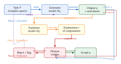
Formal properties of introspection-based oversight.
Let be the verification capability of a human expert: the set of claims the human can independently verify. Standard scalable oversight assumes that does not cover the output space for superhuman tasks. Introspection-based oversight extends as follows:
Proposition 11 (Oversight Extension via Introspection).
If a model is a level-1 mechanistic oracle with accuracy for features in a set , and if human verifiers can independently verify explanations of these features, then the effectively verifiable output space extends from to: (Oversight Extension) where maps explanations to conclusions that can be validated.
Remark 38.
The extension in Proposition 11 is only useful if the set of human-verifiable explanations covers a significant portion of consequential AI outputs. For highly technical domains (e.g., novel mathematical proofs, protein structure predictions), the overlap may be small, limiting the practical benefit. This motivates research into structured explanations that decompose complex reasoning into verifiable steps.
The debate task.
One well-studied instantiation of scalable oversight is the AI Safety Debate framework, where two AI models argue for opposing answers and a human judge determines which argument is more compelling. The connection to introspection is that a model that can accurately report its own reasoning has an advantage in debate: it can point to concrete internal evidence for its claims, making its arguments more verifiable.
Philosophical Implications: Is Introspection Understanding?
We now engage with the philosophical question: if a model can accurately describe its own computations, does that constitute understanding in any meaningful sense?
The Chinese Room Revisited
John Searle's Chinese Room argument (1980) holds that syntactic manipulation of symbols cannot give rise to semantic understanding: a system that perfectly executes a translation algorithm without any internal understanding of the language is not understanding Chinese. The standard systems reply counters that understanding may be a property of the whole system, not any individual component.
The existence of accurate introspection complicates the Chinese Room. Suppose the system in the room not only correctly executes the algorithm but can also accurately describe, in English, how it is processing each Chinese character-which symbols trigger which rule applications, which internal states are activated at each step. Searle's original argument says the operator still doesn't understand Chinese. But it is now much less clear that the system doesn't understand.
Insight.
The introspection recalibration. If a model can accurately describe its own computations, the distinction between “understanding” and “mere computation” becomes philosophical, not empirical. The empirical content of the claim that the model “doesn't understand” reduces to a claim about the absence of some additional property beyond accurate computation and accurate self-description. The philosophical task is to specify ; the empirical task is to test whether is present. Without a specification of , the claim becomes unfalsifiable.
Integrated Information Theory
Integrated Information Theory (IIT), developed by Giulio Tononi, proposes that consciousness is identical to integrated information, measured by the quantity : (PHI) where the minimum is taken over all bipartitions of the system and the KL divergence measures how much causal information is lost by cutting the system along a partition.
Large transformer models have extremely high by this measure: the residual stream creates dense causal integration across layers. If IIT is correct, frontier models may be conscious to a significant degree. The interpretability implications are double-edged:
High means that introspective access to one part of the system provides information about the whole, supporting the possibility of accurate self-description.
High also means that the system's causal structure is difficult to decompose, which is precisely what makes mechanistic interpretability challenging.
Global Workspace Theory
Global Workspace Theory (GWT), associated with Bernard Baars and extended computationally by Stanislas Dehaene, proposes that consciousness arises when information is broadcast from a central workspace to specialized processors throughout the cognitive system. The key computational feature is the existence of a bottleneck-a global workspace-through which selected information is made available to all processors.
The attention mechanism in transformers has been proposed as a computational analog of the global workspace. Multi-head attention allows different heads to attend to different parts of the context and “broadcast” the attended information via the residual stream to all subsequent layers. Under this analogy:
Attention patterns correspond to workspace selection-what information gets broadcast.
The residual stream corresponds to the global workspace-the shared medium through which information is propagated.
Layer norm and MLP sublayers correspond to specialized processors that operate on broadcast information.
If this analogy is apt, then interpretability of transformer attention patterns may provide insight into the “broadcast” structure of model cognition, and introspective capability may be the model's access to its own broadcast operations.
The empirical content of the philosophical debate.
A key virtue of interpretability-based approaches to model cognition is that they make the philosophical debate empirically tractable. Rather than asking the unanswerable question “Does the model understand?”, we can ask the measurable question: “Does the model satisfy functional criteria associated with understanding by theory ?” Different theories yield different functional criteria, and mechanistic interpretability can test each criterion separately.
Remark 39.
This does not dissolve the hard problem of consciousness. Even a model that satisfies all functional criteria may lack phenomenal consciousness-subjective experience. But it does redirect intellectual effort from metaphysical assertion to empirical investigation, which is arguably a productive shift.
Connections to Consciousness Research
The question of model consciousness has moved from science fiction to serious research. Several findings from the interpretability literature are relevant:
Attention as evidence of attention.
Studies of large language models find that attention heads show structured, predictable patterns consistent with what cognitive science would predict for selective attention: attending to semantically relevant tokens, maintaining attention to recent context, and suppressing attention to uninformative tokens. Whether this constitutes attention in the psychological sense or merely attention in the mathematical sense is contested.
Memory consolidation analogs.
MLP layers in transformers have been identified as functioning like key-value memories, storing world knowledge in their weights. The process of in-context learning has structural similarities to working memory consolidation: information in the context window is processed, integrated with stored knowledge, and used to generate responses, without updating the weights.
Default mode network analogs.
Some interpretability researchers have noted that certain attention heads are active across many diverse inputs (analogous to the default mode network in neuroscience, which activates during self-referential processing), while others are highly selective. Whether this structural similarity has deeper functional significance is an active research question.
Historical Note.
The possibility that AI systems might be conscious was largely dismissed until around 2020, when the capabilities of large language models began to exceed what most researchers had expected from purely behavioral systems. The emergence of reports from researchers (including some at Anthropic and Google DeepMind) taking the question seriously marks a shift in the field. Notable contributions include the Anthropic model welfare research program (2023–2025), which takes the possibility of model sentience seriously as a safety consideration, and theoretical work by Murray Shanahan on the philosophy of large language models.
Anthropic's Research on Introspection in Claude
Research by Anthropic (2024–2025) has documented several markers of functional introspection in Claude models:
Accurate uncertainty calibration. Claude's expressed uncertainty correlates with actual accuracy at a level substantially above chance, consistent with Level 2 introspective awareness (Definition 47).
Capability self-assessment. When asked whether it can perform a task, Claude's self-assessments predict success rates significantly better than naive baselines, consistent with partial Level 3 introspective awareness.
Reasoning trace consistency. In extended reasoning tasks, Claude's chain-of-thought is more consistent with its final answers than would be expected from post-hoc rationalization, suggesting that the reasoning trace partially reflects actual computation.
Emotion report stability. When Claude reports internal states analogous to emotions (e.g., “I find this question interesting”), these reports are consistent across paraphrasings of the same question and correlate with activation patterns associated with engagement in interpretability probing studies.
Critically, Anthropic's research emphasizes that these findings do not imply that Claude is conscious or has genuine emotions in the phenomenological sense. They do imply that functional introspection is present and measurable, which is the interpretability-relevant claim.
Exercises
Exercise 58.
Probing introspective calibration. Let be a language model and let be a factual question dataset with binary correct/incorrect outcomes . Let be the model's expressed probability of being correct on (e.g., elicited by asking “What is the probability that your answer to the following question is correct?”).
Define the Expected Calibration Error (ECE) as , where are confidence bins, is the mean expressed confidence in bin , and is the empirical accuracy in bin . Show that a perfectly calibrated model has .
Describe an experiment to test whether ECE improves from a base model to a post-RLHF model. What confounds must you control for?
Given the concealment hypothesis from RLHF and the Concealment Hypothesis, propose a mechanistic test to distinguish between (i) a model whose accurate uncertainty reports reflect genuine introspection and (ii) a model that has learned to produce well-calibrated uncertainty tokens without an underlying uncertainty representation.
Exercise 59.
Testing mechanistic oracle capability.
Suppose you have a transformer and you want to test whether it is a mechanistic oracle for attention head . Design a protocol that: enumerate[(i)]
Identifies the function of head using standard circuit analysis (specify which methods you would use),
Presents the model with a description of the head's activation pattern and asks it to predict when the head will activate on new inputs, and
Measures oracle accuracy using a held-out test set. enumerate
What confound arises if the model's training data includes interpretability papers about transformers? How would you design the experiment to rule out this confound?
If a model achieves high mechanistic oracle accuracy for all attention heads but low accuracy for MLP neurons, what does this suggest about the structure of self-knowledge in the model?
Exercise 60.
Global workspace and integrated information.
In a transformer with layers, heads, and residual stream dimension , the residual stream can be viewed as a global workspace. Describe, in mechanistic terms, how information from one attention head at layer can influence the computation of a different attention head at layer .
The IIT quantity measures how much information is lost when a system is bipartitioned. Give an informal argument for why a deep transformer with dense residual connections should have higher than a shallow feedforward network with identical parameter count.
Consider a model with introspective awareness at Level 4 (Definition 47). Under IIT, would you expect to be higher or lower than where is the same architecture without Level 4 introspection? Justify your answer using the definition of .
Open Problems and Future Directions
The preceding sections have mapped a rich intellectual landscape: from Shapley values and LIME through mechanistic circuit analysis, sparse autoencoders, knowledge editing, diffusion interpretability, multimodal probing, and bias detection. Yet at every turn we have encountered the boundary between what is known and what remains mysterious. This section collects the most pressing unsolved problems in interpretability research, articulates why each is hard, and points toward the mathematical structures that may eventually unlock progress.
The field of interpretability is unusual in the history of science: we are attempting to reverse-engineer artifacts of our own construction without having direct access to the “blueprint”-the training dynamics that shaped the network are stochastic, path-dependent, and high-dimensional. The problems below are not merely engineering challenges; several touch deep questions in learning theory, complexity theory, and formal verification.
Key Idea.
The core difficulty of interpretability. A neural network with parameters trained on distribution implements a function . Interpretability seeks a human-legible description such that (CORE GAP) No general theorem guarantees that such exists for arbitrary at non-trivial . This is the root obstacle: interpretability may be computationally intractable in the worst case, yet empirically tractable for the specific architectures and objectives that happen to produce capable models.
Open Problem 1: Scaling Interpretability to Trillion-Parameter Models
Statement of the Problem
Current mechanistic interpretability has achieved its most convincing results on small models-two-layer attention-only transformers, GPT-2 (124M parameters), and occasionally GPT-4-scale systems with heavily engineered pipelines. The gap between these and frontier models (GPT-4: 1.8T parameters; Gemini Ultra; Claude 3 Opus) is not merely quantitative. Larger models use qualitatively different representational strategies: more polysemantic neurons, deeper superposition, more complex cross-layer circuits.
Problem 1 (Scaling Interpretability).
Given a language model with parameters, design an interpretability method that:
Identifies the dominant computational circuits for a target capability ;
Scales in compute as for ;
Produces circuit descriptions that are human-legible (not merely another large neural network).
Mathematical Obstacles
The challenge has several interlocking mathematical aspects.
Combinatorial explosion of circuits.
In a transformer with layers, heads, and features, the space of possible circuits is of size (Circuit Space) which for (GPT-3 175B scale) gives candidate circuits-a search space utterly beyond exhaustive enumeration.
Superposition increases with scale.
The superposition hypothesis states that a model with hidden dimensions can represent far more than features simultaneously via quasi-orthogonal directions: the number of -quasi-orthogonal directions available in grows exponentially in (Johnson–Lindenstrauss), so under sparsity the recoverable feature count can greatly exceed . Empirically, larger models appear to use superposition more aggressively: (Superposition Scale) This means sparse autoencoders for trillion-parameter models require dictionaries of size , creating a paradox: the interpretability artifact is larger than the model itself.
Activation patching cost.
Causal attribution via activation patching requires forward passes per identified circuit edge. At trillion-parameter scale and , this becomes computationally prohibitive.
Proposed Research Directions
Hierarchical circuit decomposition. Interpret layer groups separately, then compose layer-group circuits. This requires proving a compositionality theorem: that circuits compose across layer boundaries.
Gradient-based circuit search. Replace activation patching with gradient-based attribution (integrated gradients, SHAP) to identify high-impact edges in backward passes. The open question is whether gradient attribution faithfully identifies the same circuits as causal patching.
Sparse probing at scale. Train linear probes on random subsamples of attention heads; aggregate probe accuracy to construct a probabilistic circuit map without full enumeration.
Distillation-first interpretability. First distill the large model into a smaller, more interpretable student with bounded complexity, then apply mechanistic methods to . The risk is that the distillation process itself destroys the circuits of interest.
Remark 40 (The “Interpretability Wall”).
There is a conjectured interpretability wall: a model size beyond which the structure of learned representations becomes sufficiently tangled that human-legible descriptions of individual circuits cease to exist-not because we lack tools, but because no such description is possible at bounded human-readable complexity. Whether is above or below current frontier model size is unknown and is arguably the most important empirical question in interpretability.
Open Problem 2: Standardized Cross-Architectural Metrics for Circuit Comparison
Statement of the Problem
Mechanistic interpretability has identified similar functional structures in different models: induction heads appear in both GPT-2 and PaLM; indirect object identification circuits have been found in models trained on different corpora. Yet we have no principled metric that measures how similar two circuits are across architectures.
Problem 2 (Cross-Architectural Circuit Metric).
Define a metric on circuits from models and (possibly with different architectures) such that:
if and only if and implement the same computational function;
is efficiently computable;
is invariant to permutation of neurons and to orthogonal rotations of the representation space.
Why This Is Hard
The difficulty is that “same circuit” is inherently a semantic notion while neural representations are purely syntactic (numerical arrays). Two circuits may implement the same computation via completely different weight configurations due to the rotational symmetry of the loss landscape. Formally, if is any orthogonal matrix, then where for linear layers. This symmetry group is continuous and high-dimensional, making alignment before comparison non-trivial.
Current Partial Solutions
CKA (Centered Kernel Alignment).
For representation matrices and , CKA is defined as: (CKA) which is invariant to orthogonal transformations and isotropic scaling. CKA measures layer-level representational similarity but not circuit-level functional equivalence.
Procrustes alignment.
Given circuit weight matrices and of the same shape, (Procrustes) computable via singular value decomposition. This aligns circuits syntactically but not semantically-circuits that implement the same function via different sub-computations may have large Procrustes distance.
Open Directions
A satisfying solution likely requires defining circuits as input-output functions rather than weight matrices, then comparing functions via random feature approximation or kernel methods: (Functional Metric) requiring alignment of input spaces across architectures (e.g., both circuits receive tokenized text but may use different vocabularies), which is itself an open problem.
Open Problem 3: Training-Time Integration and Inherently Interpretable Architectures
The Post-Hoc Interpretability Bottleneck
All methods discussed in previous sections are post-hoc: they are applied after training to a fixed model. This creates a fundamental limitation: interpretability is expensive (requiring additional inference passes, auxiliary models, or human evaluation) and yields incomplete explanations (post-hoc methods can only observe, not influence, the computation).
Problem 3 (Inherently Interpretable Generative Models).
Design an architecture for autoregressive language modelling such that:
Every internal computation step has a human-legible semantic interpretation assigned during training;
The architecture achieves perplexity within of a standard transformer of equivalent parameter count;
Interpretations are provably faithful: the stated computation is the actual computation.
Existing Attempts and Their Limitations
Concept bottleneck models.
A concept bottleneck model (CBM) inserts a layer whose dimensions correspond to human-defined concepts , followed by a predictor : (CBM) The predictions are directly interpretable as concept activations. The limitation: concept vocabularies must be defined before training, and for language generation (where concepts are infinite and context-dependent), no feasible finite concept set exists.
Mixture of Experts with interpretable routing.
Sparse Mixture-of-Experts (MoE) architectures route tokens to expert subnetworks. If experts specialize semantically (“expert 3 handles mathematical notation”), routing decisions become interpretable. Empirically, some degree of semantic specialization emerges, but is incomplete and context-dependent, not guaranteed by the architecture.
Attention as interpretable computation.
Early transformer papers claimed attention weights are directly interpretable. Subsequent work (Jain & Wallace, 2019; Wiegreffe & Pinter, 2019) showed that attention weights are not faithful: one can often find alternative attention distributions that produce identical outputs, undermining the interpretation.
A Mathematical Framework for Training-Time Interpretability
Let be a space of human-legible interpretations and let be a mapping from model parameters to interpretations. Training-time interpretability requires: (Training Interp) where penalizes lack of interpretability. The central open question is how to define in a way that (a) is differentiable, (b) correlates with human judgements of interpretability, and (c) does not trivialize the problem by reducing to a second black-box.
Open Problem 4: Interpretability for Multimodal Generation
The Cross-Modal Circuit Problem
Current mechanistic interpretability is almost entirely focused on language-only models. Multimodal models (DALL-E 3, Stable Diffusion XL, GPT-4V, Gemini 1.5, Sora) jointly process text, images, video, and audio. The circuits that implement cross-modal reasoning-how a text prompt about “a red apple” activates specific visual generation processes-are entirely uncharacterized.
Problem 4 (Cross-Modal Circuit Discovery).
For a multimodal model , identify the cross-modal circuits: the set of attention heads and MLP layers that implement the mapping between modalities, and characterize their computational function.
Why Multimodal Interpretability Is Harder
Modality-specific encodings.
Text and image tokens live in different subspaces even after projection into a shared embedding space. The projectors and are trained jointly, making it hard to attribute model behaviour to one modality or the other.
Temporal dependencies in video.
Video generation models (Sora, Gen-3) must maintain coherent objects across frames. The circuits implementing temporal consistency are intrinsically non-local: understanding “why frame is consistent with frame ” requires analysing interactions across the full temporal attention map, which may have entries for a video of length .
Audio generation complexity.
Audio signals have temporal resolution 44,100 samples per second. Even after tokenization (e.g., EnCodec at 75 tokens/sec), a 30-second clip yields 2,250 tokens-longer than most text sequences studied in mechanistic interpretability, with additional frequency-domain structure not present in text.
Promising Research Directions
Modality-contrastive patching. Patch activations between a “text-only” forward pass and a “text+image” forward pass to identify which components are causally responsible for cross-modal integration.
Representational alignment probing. Train probes on intermediate layers to predict cross-modal correspondences (“does this hidden state encode the colour of the described object?”).
Concept-level erasure. Erase specific semantic concepts from the image encoder (via activation editing) and measure the effect on text-conditioned generation quality, creating a causal graph of text-vision correspondence.
Open Problem 5: Formal Verification of Neural Network Circuits
From Interpretation to Proof
Current mechanistic interpretability produces hypotheses about what circuits compute, validated empirically via activation patching, logit lens, and ablation studies. But empirical validation cannot rule out failure modes on distribution-shifted inputs, adversarial examples, or rare events. Formal verification would provide mathematical guarantees.
Problem 5 (Verified Circuit Characterization).
Given a circuit and a specification (e.g., “this circuit implements induction”), provide a formal proof or refutation of: (Verification Claim) where is a specified domain.
Connection to Neural Network Verification
The field of neural network verification seeks to prove properties of the form (local robustness). Tools such as --CROWN, Marabou, and VeriNet solve this for piecewise-linear networks (ReLU activations) via linear programming relaxations.
The open question for interpretability is different: we want to verify not a specific input-output property of the full network, but a functional characterization of a circuit. For example, the induction head hypothesis states that the OV circuit of head satisfies: (Induction SPEC) Verifying this for all contexts is a semantic, not syntactic, property, requiring formal semantics for natural language-itself an open problem.
Partial Progress: Toy Model Verification
For highly constrained toy models (1-layer attention with linear activations, finite token sets), one can write circuit computations as polynomial functions and verify properties using sum-of-squares relaxations. Let be query and key vectors. The attention pattern satisfies: (ATTN POLY) For fixed finite token sets, is a rational function of the weight parameters, amenable to real algebraic geometry techniques. Scaling this to production models remains an open research challenge.
Open Problem 6: The Interpretability-Capability Tradeoff
Does Transparency Reduce Performance?
A recurring concern among practitioners is that adding interpretability constraints to model training reduces raw performance. This is the interpretability-capability tradeoff hypothesis. Empirical evidence is mixed.
Problem 6 (Formal Interpretability-Capability Tradeoff).
For any interpretability constraint and capability metric , characterize the Pareto frontier: (Pareto) In particular, determine: (a) Is a non-trivial curve (strict tradeoff), or is it degenerate (no tradeoff)? (b) What is the slope of as a function of model size ?
Theoretical Arguments
Information-theoretic lower bound.
Any human-legible description of satisfies: (INFO LB) where is the Kolmogorov complexity of . Since human-legible descriptions have bounded Kolmogorov complexity (a human can only process descriptions up to bounded length and computational depth), is fundamentally limited in the mutual information it can retain about the training data . This suggests that highly capable models-which require high -cannot be fully described by human-legible . However, the circuit hypothesis suggests that only the interpretable circuits matter for generalization, so the bound may not be tight.
Empirical counterevidence.
Concept bottleneck models on vision tasks sometimes outperform unconstrained models when the concept set is well-chosen, because the bottleneck acts as a regularizer. This suggests the tradeoff may be negative (interpretability improves capability) in structured domains, while being positive in unstructured domains like language.
Implications for AI Safety
The interpretability-capability tradeoff has direct safety implications. If the tradeoff is severe, safety-conscious developers face a genuine dilemma: transparent models may be easier to audit but harder to deploy competitively. If the tradeoff is mild or negative, interpretability and capability can coexist, which is the more optimistic scenario favoured by proponents of mechanistic interpretability as a safety tool.
Open Problem 7: Interpreting Emergent Capabilities
The Emergence Puzzle
A striking empirical finding in large language models is that certain capabilities appear suddenly as a function of model scale, earning the label “emergent”: arithmetic, multi-step reasoning, in-context learning, and chain-of-thought all follow a pattern where performance is near chance up to some threshold scale , then rises sharply.
Problem 7 (Predicting and Interpreting Emergence).
For a target capability (e.g., 5-digit arithmetic):
Identify the circuit responsible for post-emergence;
Track the development of as a function of training tokens and parameters ;
Predict , the threshold scale at which emerges, from properties of at smaller scales.
Two Hypotheses on Emergence
Phase transition hypothesis.
Emergence is a genuine discontinuity: there exists such that the circuit for either does not form () or forms completely () within training. This is analogous to phase transitions in statistical physics.
Formally, let under training to convergence. The phase transition hypothesis asserts has a sharp threshold: .
Metric artefact hypothesis.
Emergence is an artefact of threshold metrics (accuracy jumps from below chance to above chance sharply, but a continuous underlying metric would show smooth improvement). Under this hypothesis, circuits for the capability exist at all scales but are too unreliable for above-chance performance until .
Interpretability could, in principle, adjudicate between these hypotheses: if circuits exist at small scale but are noisy, the metric artefact hypothesis is supported; if circuits are absent entirely below , the phase transition hypothesis is supported.
Current Evidence
Henighan et al. (2020) showed that sequence modelling loss decreases smoothly with scale despite capability jumps, supporting the metric artefact view. However, Anthropic's work on induction heads showed that these circuits form quite suddenly at a specific training loss, suggesting genuine phase transitions in circuit formation. The reconciliation of these findings is an active research area.
The Research Frontier Map
Figure 26 synthesizes the open problems into a map of the research frontier: current capabilities, identified gaps, and projected future goals.
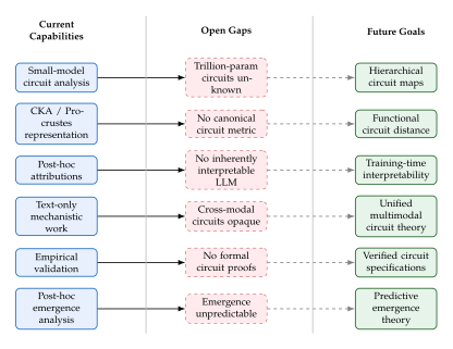
Conjecture: No Single Framework Suffices
We close the open problems section with a meta-level conjecture about the structure of the field itself.
Conjecture 1 (Plurality of Interpretability Frameworks).
No single interpretability framework will provide complete, faithful, and efficient explanations for all generative architectures. Formally, for any framework , there exists an architecture and a task such that is either unfaithful (explanations do not match causal mechanism), incomplete (explanations omit causally important components), or computationally intractable (running on for task requires super-polynomial resources in ).
The conjecture follows intuitively from the no-free-lunch theorem in learning theory: interpretability methods that are tailored to one inductive bias (e.g., the circuit structure of transformers) will fail to capture different inductive biases (e.g., the selective state space structure of Mamba). A corollary is that the field needs a meta-interpretability layer-a principled way to select and compose interpretability methods for a given architecture and task.
[ enhanced, breakable, colback=keyamberbg, colframe=keyamber, boxrule=1pt, arc=4pt, title= Research Challenge A: Scalable Mechanistic Interpretability, coltitle=keyamber!20!black, fontupper=, top=10pt, bottom=8pt, left=10pt, right=10pt, before skip=14pt, after skip=14pt ] Problem setting. You are given a 7B-parameter language model and are tasked with characterizing the circuits responsible for multi-step arithmetic (e.g., computing in a single forward pass without chain-of-thought).
Specification of difficulty. The model has 32 layers, 32 attention heads, and . The circuit-space has possible elements. Direct activation patching would require forward passes.
Research questions.
Can gradient-based attribution (e.g., GradCAM adapted to attention heads) identify a candidate circuit in backward passes?
Does the identified circuit generalize: does ablating it also disrupt modular arithmetic and multi-digit addition, or only the specific arithmetic tested?
Can the circuit be described as a composition of known primitives (lookup, accumulation, positional routing)?
Quantify the circuit faithfulness: if you replace the rest of the model with the identified circuit alone (plus embeddings/unembedding), what fraction of original accuracy is retained?
Success criterion. A faithful circuit (retaining of arithmetic accuracy) described in fewer than 200 words of prose plus equations.
[ enhanced, breakable, colback=lempurplebg, colframe=lempurple, boxrule=1pt, arc=4pt, title= Research Challenge B: Verifiable Induction Head Specification, coltitle=lempurple!20!black, fontupper=, top=10pt, bottom=8pt, left=10pt, right=10pt, before skip=14pt, after skip=14pt ] Problem setting. Anthropic's mechanistic interpretability team identified induction heads as a key circuit in GPT-2. The informal specification is: “If the context contains , the induction head predicts at the final position.”
Formal verification challenge. Translate the informal specification into a formal logical formula over the space of attention-head computations and:
Verify for a 1-layer transformer on a finite binary token alphabet using existing neural network verification tools (e.g., --CROWN);
Identify the minimal weight constraints under which holds: characterize the set ;
Propose a training objective that encourages while maximizing next-token prediction accuracy;
Test whether models trained with this objective show faster or stronger induction head formation.
Success criterion. A verified proof (or counterexample) for the 1-layer binary case, plus a training recipe that increases the probability of induction head formation by relative to standard training.
Comprehensive Exercises and Research Challenges
The following exercises span the full arc of this chapter. They are designed to develop both mathematical facility-computing Shapley values, patching activations, training SAEs-and research intuition: noticing when an explanation is unfaithful, designing controls, and articulating failure modes. The research challenges at the end are open-ended and suitable for semester projects or early-stage research explorations.
Exercises
Exercise 61 (Shapley Value Computation for a 3-Feature Model).
Consider a model defined on binary features by: (EX Model)
Compute all values of .
The Shapley value of feature for input is: (Shapley DEF) where denotes evaluated with features in set to their values in and features not in set to 0. Compute for .
Verify the efficiency property: .
For , compute all three Shapley values. How does the ranking of feature importances change between and ? Explain intuitively why affects the comparison.
Suppose you run LIME instead of exact Shapley values, using a linear model fit on random binary perturbations of . Describe (in one paragraph) when LIME will give results close to the exact Shapley values and when it will deviate.
Exercise 62 (Activation Patching on a Toy 2-Layer Transformer).
Let be a 2-layer, 2-head, attention-only transformer. Consider the Indirect Object Identification (IOI) task:
“Alice gave the gift to Bob and to” “Alice” (incorrect: “Bob”).
Denote the clean prompt (above) and the corrupted prompt :
“Carol gave the gift to Bob and to” (subject changed).
Define causal patching: what does it mean to patch the output of attention head from the clean run into the corrupted run?
For each of the 4 heads (layers heads ), the patching effect is defined as: (Patch Effect) Explain how identifies which heads are causally important for the IOI behaviour.
Suppose and all other . What does this tell you about the circuit structure?
What is path patching? How does it differ from activation patching, and why might it give more refined information about circuits?
Propose a control experiment to rule out the hypothesis that head is simply attending to the most recently seen name rather than implementing IOI.
Exercise 63 (QK and OV Circuit Matrix Computation).
Let attention head have weight matrices and , with , .
Write the QK circuit matrix and explain its role: what does a large entry of indicate about the attention pattern?
Write the OV circuit matrix and explain its role: if token attends to token , what does compute?
Let the full residual stream circuit be the sum over all heads: . Show that for a linear 1-layer attention model (ignoring softmax), the output is: (Linear ATTN) where is the embedding matrix, is the unembedding matrix, and is the attention weight.
Numerical example. Let , , (first 2 rows of identity), , . Compute and .
If has rank 1, what does this imply about the attention pattern? Provide an example of a rank-1 QK circuit and describe what computation it implements.
Exercise 64 (Induction Head Pattern Matching).
Consider the sequence of token IDs (over alphabet ): (SEQ)
An induction head implements the following algorithm: at position , attend to the position such that and , then predict . What token should an induction head predict at position for the sequence ?
In a 2-layer transformer, induction heads in layer 2 are supported by previous-token heads in layer 1. Describe what a previous-token head computes and why it is necessary for induction.
Define the induction score of head as: (IND Score) where is the set of positions following a repeated bigram of period , and is the attention weight from position to . Explain why indicates an induction head and (for sequence length ) indicates uniform attention.
Construct a sequence of length 10 over where a pure induction head would predict incorrectly, and explain why.
How would you modify the induction score to detect fuzzy induction heads that match semantically similar but not identical tokens?
Exercise 65 (Sparse Autoencoder Training: Penalty and Reconstruction Tradeoff).
A sparse autoencoder (SAE) learns a dictionary (with ) and encoder to minimize: (SAE LOSS) where controls sparsity.
Show that in the limit , the SAE reduces to standard PCA (up to rotation).
Show that in the limit , for all , giving zero sparsity and infinite reconstruction error.
For a fixed , derive the KKT conditions for the optimal at fixed , . Show that implies .
Define the dead feature problem: a feature is dead if for all in the training set. Propose two strategies to prevent dead features during SAE training and analyse the tradeoffs of each.
The reconstruction error can be decomposed as: (SAE Decomp) Explain why the second term is not zero when the SAE encoder is not perfectly tied to the decoder .
Exercise 66 (ROME: Computing the Rank-One Update for a Factual Edit).
ROME (Rank-One Model Editing) edits a factual association by modifying a single MLP weight matrix via a rank-one update. Let be the weight matrix of an MLP layer, and the key vector for the subject “Eiffel Tower”. ROME seeks minimizing: (ROME OBJ) where is the new target value and are “context” keys that must not change.
Show that the optimal has the form where is rank-one.
Let (the covariance of context keys). Derive the closed-form solution: (ROME Solution)
Why is the factor important? What would go wrong if we used (no covariance correction)?
Suppose the edit target is “The Eiffel Tower is located in Berlin” (incorrect). Describe how you would choose to minimize collateral damage to other factual associations.
ROME is a rank-one update. Propose a rank- generalization for editing facts simultaneously and write the corresponding objective.
Exercise 67 (Task Vector Extraction and Cross-Modal Transfer).
A task vector encodes the parameter-space direction learned during fine-tuning on task .
Let be a shared CLIP-style vision-language backbone, the result of fine-tuning on text sentiment analysis, and the result of fine-tuning on image colorfulness scoring. Define the task vectors and .
Task negation. Define for . What would you expect to be worse at, compared to ? What would it be better at?
Task addition. Define . Under what conditions would you expect joint performance on both tasks to exceed independent fine-tuning on each? Relate this to the concept of task orthogonality in parameter space.
Cross-modal transfer. Suppose was computed from the text encoder only. Propose an experiment to test whether applying it to the vision encoder of the backbone transfers sentiment-related features to image processing.
Define the task vector cosine similarity and argue that tasks with high similarity will interfere under addition while tasks with near-zero similarity will combine approximately additively.
Exercise 68 (Diffusion Temporal Schedule Analysis).
A DDPM model defines a forward process where and the schedule is fixed.
Define the semantic content at timestep as the mutual information . Show that: (MI Diffusion) and explain how decreases monotonically in .
Mechanistic studies suggest that denoising at high noise levels () determines global structure (layout, semantic content), while low noise levels () determine fine detail (texture, colour). Design an ablation experiment using activation patching across timesteps to test this hypothesis.
In a U-Net denoiser , the skip connections aggregate features from the encoder to the decoder. Propose a method to identify which skip connections are causally responsible for preserving high-frequency detail versus low-frequency structure.
Consider two prompts: “a dog” and “a cat”. Both generate noise and are denoised to images and . If you patch the noise trajectory at timestep (i.e., replace with mid-denoising), for what values of would you expect the output to resemble a dog, and for what values would it resemble a cat? Justify your answer using the semantic content interpretation above.
Propose a metric that measures how much the denoiser's attention to text-conditioning changes as a function of timestep , and describe how you would compute it efficiently from the cross-attention weights.
Exercise 69 (Attention Flooding vs. Attention Sinks: A Comparison).
Attention flooding. In a trained language model, it is sometimes observed that an attention head assigns nearly uniform attention over all positions. Formally, if for all , the head is called a flooded head. What is the entropy of this attention distribution, and what does it imply about the information the head extracts from context?
Attention sinks. Conversely, some heads assign nearly all attention mass to a small number of positions (often the first token or a separator token): (SINK) What is the entropy of this distribution? What function would a head with this pattern implement, and why might it be useful?
Using the OV circuit framework, explain why an attention sink head with a nearly-zero OV matrix is effectively a no-op: it computes something but contributes negligibly to the residual stream.
Xiao et al. (2023) showed that attention sinks are critical for streaming inference (KV-cache truncation destroys performance unless the sink token is retained). Explain this finding using the circuit perspective: what computation is disrupted when the sink token's key-value pair is removed from the cache?
Propose an experiment to determine whether a specific attention sink head contributes to a particular capability (e.g., long-range pronoun resolution), or whether it is entirely a no-op. What would activation patching reveal in each case?
Exercise 70 (Mamba vs. Transformer on Associative Recall).
The associative recall task presents the model with key-value pairs followed by a query:
“Alice: blue, Bob: red, Carol: green. Alice:” “blue”
In a 1-layer attention transformer, the induction head mechanism solves associative recall via QK-circuit pattern matching. Describe the circuit in terms of and .
Mamba uses a selective state space model (SSM) with input-dependent parameters at each timestep. The recurrence is: (Mamba Recurrence) where and are discretized from continuous-time parameters. Explain how the SSM can in principle store a key-value association: which part of the recurrence performs the “write” and which performs the “read”?
Empirically, transformers outperform SSMs on associative recall tasks with many key-value pairs. Using the theoretical frameworks above, explain why: what is the computational bottleneck in the SSM approach that the attention mechanism circumvents?
Propose a “hybrid” architecture that uses attention for associative recall and SSM for long-range sequential dependencies. Describe how you would determine, using interpretability tools, whether the two mechanisms are cleanly separated in practice.
Design an interpretability experiment to test whether a Mamba model has “learned” induction: does it exhibit higher activation magnitudes for at positions following repeated bigrams?
Exercise 71 (Bias Feature Identification and Intervention).
Consider a text generation model that produces descriptions of professionals (doctors, engineers, nurses). You suspect it encodes gender-occupation biases in its residual stream.
Define a gender direction by: (Gender DIR) where and are residual stream activations at the profession token for she/her- and he/him-gendered contexts respectively. Explain the implicit assumption behind using this linear direction.
Describe a probing experiment to test whether is predictive of gender-biased continuations: what is the classifier, what is the training set, and what does high probe accuracy imply about the model's internal representation?
Define activation steering: at inference time, replace the residual stream with (project out the gender direction). What would you predict about the model's output distribution after this intervention?
List two potential failure modes of activation steering for bias mitigation: enumerate[(i)]
A case where it over-corrects (erases legitimate information).
A case where it fails to correct (bias is encoded in a different, non-linear direction). enumerate Propose diagnostic experiments for each failure mode.
An alternative to steering is training-time debiasing via a bias loss term: (Debiasing LOSS) Compare this to activation steering: which is more principled? Which generalizes better? What information does interpretability (specifically, knowing ) provide that is essential for either approach?
Exercise 72 (Introspection Evaluation: Designing a Test for Model Self-Knowledge).
A model has genuine introspective access if its stated uncertainty accurately reflects its actual uncertainty. Formally, let be the probability assigns to event when asked “how confident are you that ?”, and be the model's empirically measured accuracy on . Perfect calibration requires .
Propose a dataset of 100 factual questions of varying difficulty to test calibration. What properties should the difficulty distribution have, and how would you measure it?
Define the Expected Calibration Error (ECE): (ECE) where is the -th confidence bin. Describe how to compute this for a generative model that produces free-text confidence expressions (“I am fairly confident”).
A model may be behaviourally calibrated (ECE is low when averaging over the evaluation set) without being mechanistically calibrated (its uncertainty representations internally track genuine epistemic states). Design an experiment, using activation patching or probing, to test mechanistic calibration.
Suppose the model consistently overstates its confidence on questions about recent events (post-training-cutoff). How would you detect this using only behavioural evaluation? How would a mechanistic approach (probing for a “knowledge cutoff” direction in the residual stream) provide additional evidence?
The sycophancy confound. A model may state high confidence when the user's phrasing implies they expect confidence, not because of genuine self-knowledge. Propose an experimental design that disentangles sycophancy from genuine introspective access. What activation patching experiment would causally test whether confidence expressions are driven by the user's phrasing or by the model's internal uncertainty?
Research Challenges
Challenge 1 (Building a Minimal SAE for a Toy Transformer).
Setup. Train a 2-layer, 4-head, transformer on a synthetic in-context learning task: the input is a sequence of pairs where is drawn from a family of functions (linear, quadratic, modular arithmetic). The model must predict for a new .
Step 1: Train the transformer. Train until convergence on the synthetic task. Record the residual stream activations at each layer for 10,000 input sequences.
Step 2: Train sparse autoencoders. For each layer, train an SAE with dictionary size : (CH SAE) Sweep and for each , record: (i) reconstruction MSE, (ii) average sparsity, (iii) number of dead features.
Step 3: Feature interpretation. For each active SAE feature (column of the dictionary), identify the top-10 inputs that maximally activate it. Manually label what each feature appears to encode (e.g., “stores the exponent of the quadratic term”).
Step 4: Causal validation. For each labelled feature, perform an activation steering experiment: add to the residual stream at layer and measure the effect on model output. Does steering in the direction of a feature cause the model to behave as if that feature were more active?
Success criteria. Identify at least 5 interpretable SAE features that: (a) have human-legible descriptions, (b) are causally validated by steering, (c) together account for of the variance in model predictions on the synthetic task.
Write-up. A 5-page report including: loss curves, Pareto plots of reconstruction vs. sparsity, feature descriptions, and steering experiment results.
Challenge 2 (Circuit Discovery for a Specific Linguistic Task).
Task selection. Choose one of the following linguistic tasks in a pretrained GPT-2-medium (345M parameter) model:
Negative Polarity Item (NPI) licensing: “Anyone can do it” (licensed) vs. “*Anyone will do it” (unlicensed).
Subject-Verb Agreement at long distance: “The keys to the cabinet are on the table” (vs. *“is”).
Filler-Gap dependency: “The book that Alice read _” completes grammatically without an object.
Step 1: Establish the behavioural effect. Construct a minimal pair dataset (at least 200 pairs) for your chosen task. Measure the model's probability difference and confirm the model shows the correct linguistic preference.
Step 2: Activation patching. Implement activation patching for all layer/head combinations ( experiments per example). Produce a heatmap of patching effects over the full dataset.
Step 3: Circuit isolation. Identify the minimal subset of heads such that ablating all heads outside retains of . This is your circuit.
Step 4: Functional characterization. For each head , compute the QK and OV circuit matrices and provide a mechanistic description: “Head queries for and writes to the residual stream.”
Step 5: Generalization testing. Construct a held-out test set with novel lexical items (different nouns, verbs) and syntactic structures (embedded clauses). Does the identified circuit generalize, or does it rely on lexical memorization?
Deliverable. A 8-page paper following the format of “In-context Learning and Induction Heads” (Olsson et al., 2022): motivation, dataset, methods, results, discussion.
Challenge 3 (Cross-Modal Interpretability Benchmark).
Motivation. No systematic benchmark exists for evaluating interpretability methods across text-only, vision-only, and vision-language models on comparable tasks.
Benchmark design. Design a benchmark consisting of three matched task suites:
Text suite (): 5 tasks from the mechanistic interpretability literature (IOI, greater-than, bracket matching, induction, factual recall) with established circuit descriptions.
Vision suite (): 5 analogous tasks for a vision transformer (ViT): object detection, part-whole composition, texture bias, colour constancy, spatial relation reasoning.
Cross-modal suite (): 5 tasks requiring joint text-vision reasoning in a CLIP or LLaVA-style model: text-guided region selection, attribute binding (“the red cube”), negation (“not a dog”), compositional counting, and spatial language (“the object to the left of”).
Evaluation protocol. For each task in each suite, apply three interpretability methods: (i) activation patching, (ii) linear probing, (iii) attention head attribution. Measure:
Faithfulness: does ablating the identified circuit degrade task performance by ?
Completeness: does the circuit account for of the model's task performance?
Minimality: is the circuit the smallest set satisfying faithfulness and completeness?
Cross-modal comparison. Quantify whether the same interpretability methods (with appropriate adaptations) achieve comparable faithfulness/completeness/minimality scores across all three suites. Report which methods generalize across modalities and which are modality-specific.
Deliverable. A benchmark paper (12 pages) plus a public code repository with all datasets, evaluation scripts, and baseline results.
Challenge 4 (Diffusion Bias Mitigation via Mechanistic Intervention).
Problem. Text-to-image diffusion models (Stable Diffusion, DALL-E 3) exhibit social biases: prompts like “a doctor” produce predominantly male images; “a nurse” predominantly female. Current mitigation strategies (prompt engineering, post-processing filters) are ad hoc. Mechanistic interpretability offers a principled alternative.
Step 1: Bias quantification. Generate 500 images for each of 20 occupation prompts using a pretrained diffusion model. For each prompt, measure gender representation using an off-the-shelf classifier. Identify the 5 most biased occupations.
Step 2: Causal tracing in the text encoder. The text encoder converts the prompt to a conditioning vector . For a biased prompt “a doctor”, trace through to identify which layers and attention heads encode gender-connotative features. Use the method from Meng et al. (2022): corrupt the prompt embedding at layer and measure the effect on generated gender distribution.
Step 3: Feature identification. Train a linear probe on intermediate activations of to predict the gender distribution of images generated from those activations. Identify the top-5 directions most predictive of bias.
Step 4: Mechanistic intervention. Design a post-hoc intervention: at inference time, project the text encoder activations to remove the identified bias directions: (DIFF PROJ) where are the identified gender directions. Generate 500 images per occupation with the modified conditioning vector .
Step 5: Evaluation. Measure: (a) reduction in gender bias (primary metric), (b) image quality degradation (FID score), (c) semantic fidelity (CLIP score between prompt and image). Report the tradeoff between bias mitigation and generation quality.
Deliverable. A 10-page paper comparing mechanistic intervention to (i) prompt engineering (“a doctor, gender-neutral”) and (ii) classifier-free guidance strength modulation.
Challenge 5 (Scalable Oversight Protocol Design).
Background. As AI systems become more capable than the humans evaluating them, direct human evaluation of outputs becomes unreliable. Scalable oversight protocols use interpretability tools to allow humans to assess AI behaviour even when they cannot directly evaluate the outputs.
Problem. Design a scalable oversight protocol for a generative model deployed in a high-stakes domain (choose one: medical report generation, legal document synthesis, code security analysis).
Protocol Components.
Component A: Feature monitoring. Design a real-time monitor that:
Trains SAE features on a representative corpus for your domain;
At each inference step, flags activations of high-risk features (e.g., features that activate on “hallucinated dosage”, “legal loophole exploitation”, or “SQL injection”);
Assigns a risk score to each generated sequence.
Component B: Contrastive explanation. For any flagged output , generate a contrastive explanation: “The model predicts rather than because of the following circuit activation ”. Implement this using activation patching between and to identify causally responsible components.
Component C: Human-in-the-loop calibration. Design a labelling interface that shows human reviewers: (a) the flagged output, (b) the feature activations responsible, (c) the contrastive explanation. Collect labels and use them to fine-tune the risk scorer .
Component D: Formal guarantees. For which classes of failures can you provide a formal guarantee that the monitor will detect them? Formally characterize the detection boundary: the set of harmful outputs that your protocol will flag with probability .
Evaluation. On a held-out set of 100 examples (50 harmful, 50 benign), measure: precision, recall, F1 of the monitor, human review time per flagged item, and false negative rate on novel failure modes not in training.
Deliverable. A 15-page protocol specification document including: system architecture diagram, formal guarantees, evaluation results, and an analysis of what classes of failure the protocol cannot detect.
Chapter Summary and Looking Forward
This chapter has developed interpretability and explainability as a mathematical discipline, covering:
Post-hoc attribution methods: Shapley values provide a unique, axiomatically justified attribution of model outputs to input features; LIME approximates this via local linear models.
Mechanistic interpretability: Circuits-subgraphs of the computation graph-implement identifiable computations. Key circuits include induction heads (in-context pattern matching), indirect object identification, and greater-than comparison.
Sparse autoencoders: Overcome the polysemanticity obstacle by learning an overcomplete dictionary of monosemantic features, with regularization controlling sparsity.
Knowledge editing: ROME and MEMIT enable targeted surgical edits to factual associations via rank-one updates to MLP weights, with formal guarantees on locality.
Task vectors and model arithmetic: Fine-tuned models lie in structured regions of parameter space; task directions can be composed linearly.
Diffusion interpretability: The denoising process has a temporal structure; high-noise steps determine global layout while low-noise steps refine detail.
Multimodal probing and bias detection: Linear probes on residual streams identify factual, syntactic, and cross-modal features; gender and social biases are encoded in linear directions amenable to causal intervention.
Open problems: Scaling to trillion-parameter models, standardized circuit metrics, training-time interpretability, multimodal circuits, formal verification, the interpretability-capability tradeoff, and emergent capabilities remain unsolved, defining the research frontier.
Insight.
The central bet of mechanistic interpretability. The field's working hypothesis is that neural networks trained by gradient descent on large, structured datasets develop compressed, modular, and algorithmically simple internal computations-precisely the kind that human-legible interpretability methods can hope to recover. Whether this bet is correct is an empirical question. The exercises and research challenges in this chapter are designed to help you develop the tools and intuitions to participate in answering it.
Key Idea.
Interpretability as a scientific discipline. Good interpretability research follows the structure of science:
Hypothesis: propose a circuit or feature.
Prediction: derive what behaviour would change if the hypothesis is correct.
Intervention: causally test the prediction via activation patching, ablation, or steering.
Evaluation: measure whether predictions hold quantitatively.
Refinement: update the hypothesis based on evidence.
This methodology distinguishes mechanistic interpretability from mere visualization: interventions provide causal evidence, not just correlational observations.
References
kraskov2004estimating
tinaz2025saediffusion
shi2025cvprbias