39 Generative Models for Weather Prediction
“The atmosphere is a chaotic symphony of molecules, yet we dare predict its song days in advance.”
On August 29, 2005, Hurricane Katrina made landfall near Buras, Louisiana, as a Category 3 storm with sustained winds of 205 kilometres per hour. The storm surge, peaking at nine metres along the Mississippi coast, overwhelmed the levée system protecting New Orleans. Roughly 1,800 people lost their lives; economic damage exceeded $125 billion, making Katrina the costliest natural disaster in United States history up to that point. Yet the storm itself was not a surprise. Five days before landfall, the European Centre for Medium-Range Weather Forecasts (ECMWF) model had already shown a coherent Gulf of Mexico track. The US National Hurricane Center issued watches and warnings 36 hours ahead-well within the window for organised evacuation. What failed was not weather science; it was the translation of probabilistic forecast information into decisive action.
Nearly two decades later, in September 2024, Hurricane Hel\-ene swept across Florida's Big Bend coast, then tracked hundreds of kilometres inland before devastating the Appalachian communities of western North Carolina. Asheville, far from any coastline and nestled between mountain ridges, received over half a metre of rain in 48 hours; the French Broad River crested at a record 7.3 metres above flood stage. More than 200 people died. Yet the operational forecast guidance-from both traditional Numerical Weather Prediction (NWP) models and the new generation of machine-learning weather models, including GraphCast and Pangu-Weather-had correctly identified the extreme rainfall potential days in advance. The fundamental scientific challenge of predicting these events had, in large measure, been solved.
The story of Katrina and Helene illustrates the astonishing progress of weather forecasting over the past half-century, and simultaneously reveals where the remaining gaps lie. Forecasting the track of a major hurricane is no longer the primary challenge; forecasting the distribution of possible impacts-the tail of the rainfall distribution, the compound flooding risk, the probability of any given neighbourhood seeing sustained winds above 50 metres per second-remains difficult, consequential, and, as we shall see, precisely the problem for which generative models offer transformative potential.
This chapter tells the story of how generative artificial intelligence entered one of the most practically important and scientifically demanding prediction problems humanity faces: the state of the atmosphere. We develop the mathematical foundations, survey the landmark models, analyse the theoretical guarantees and known failure modes, and situate weather prediction within the broader landscape of this book. The chapter connects directly to the physics-constrained PDE modelling of Chapter 35 and draws on the interpretability tools of Chapter 38; it will also prepare the ground for subsequent chapters on geophysical and climate modelling.
The Challenge of Atmospheric Prediction
Why Weather Forecasting Matters
Weather is not merely a backdrop to human activity; it is one of the principal drivers of the global economy. A landmark 2009 analysis by the United States Weather Research Programme estimated that weather-sensitive economic sectors account for roughly one third of US GDP, approximately $3 trillion annually. Scaling globally, the weather-sensitive share of the world economy exceeds $5 trillion per year.
The channels through which weather affects economic value are diverse and sometimes surprising:
Agriculture. Approximately 80% of the variability in US crop yields is attributable to weather, principally temperature and precipitation anomalies during sensitive phenological windows. A three-day forecast of a late frost can allow a Florida citrus grower to activate smudge pots and save an entire harvest. Sub-seasonal to seasonal forecasts of El Niño–Southern Oscillation (ENSO) events allow commodity traders, insurance underwriters, and government food security programmes to hedge risks months in advance.
Aviation. The US Federal Aviation Administration estimates that weather causes approximately 70% of all National Airspace System delays, costing the airline industry over $4 billion per year in direct operating costs. Turbulence-related injuries cause more than 30 severe injuries annually in the US alone; clear-air turbulence, which leaves no visual signature and cannot be detected by airborne radar, is a particular concern as a warming atmosphere alters upper-level wind shear patterns.
Energy. The rapid expansion of wind and solar generation has made weather forecasting central to grid operation. Electricity demand peaks with temperature extremes; solar output varies with cloud cover on timescales of minutes; offshore wind turbines must be shut down in extreme conditions to prevent mechanical damage. A 1% improvement in day-ahead wind power forecast accuracy across the European grid has been estimated to save $100 million annually in balancing costs.
Disaster preparedness. The World Meteorological Organisation estimates that improved early warning systems for weather-related hazards could save 2 billion euros per year in disaster losses across Europe alone. Globally, the mortality from tropical cyclones has decreased dramatically since the 1970s-from roughly 3 deaths per 100,000 population to under 0.5-primarily due to improved track forecasts and warning lead times. Economic losses, however, continue to grow as population and infrastructure expand into vulnerable coastal zones.
Key Idea.
Weather Forecasting as a Societal Infrastructure Weather forecasting is among the most valuable publicly-funded scientific activities. The ECMWF estimates that every $1 invested in operational weather services generates $6–10 in economic value. The transition to AI-augmented forecasting is not merely a technical curiosity; it is a question of how much of this value can be preserved, and potentially multiplied, as the global forecast system undergoes its most significant architectural change in seventy years.
A Philosophical Hook: Predicting Chaos
The atmosphere contains approximately molecules. Their collective behaviour is governed by the laws of classical mechanics and thermodynamics, combined with the transfer of radiation, the microphysics of cloud droplet nucleation, and the turbulent mixing of the planetary boundary layer. No computer will ever simulate this system at the molecular scale; even a description at the kilometre scale requires resolving grid cells, each carrying dozens of physical variables, over thousands of time steps.
And yet, we predict. Not perfectly-the atmosphere is chaotic, and perfect prediction is provably impossible beyond a finite horizon-but usefully. A modern medium-range forecast for surface temperature is accurate to within about 2 degrees Celsius at seven days lead time, a level of skill that would have seemed miraculous to the meteorologists of the 1960s.
The philosophical tension is acute: the atmosphere obeys deterministic physical laws (the Navier–Stokes equations, thermodynamics, Maxwell's equations for radiation), yet its long-term behaviour is unpredictable in any practical sense. How do we navigate between the rock of determinism and the hard place of chaos?
The answer, as Edward Lorenz showed in 1963, is that determinism and unpredictability are not mutually exclusive. Tiny differences in initial conditions-differences smaller than any measurement can detect-grow exponentially in time, eventually overwhelming the signal. This is the celebrated butterfly effect: the metaphorical flap of a butterfly's wings in Brazil can, in principle, alter whether a tornado forms in Texas three weeks hence. The practical implication is that there exists a fundamental predictability horizon beyond which deterministic single-valued forecasts become useless, and the only honest statement is a probability distribution over possible atmospheric states.
This insight, which we will formalise below, is the philosophical foundation for everything that follows in this chapter. Weather forecasting is, at its core, a problem of learning and sampling from a conditional probability distribution-precisely the kind of problem generative models are designed to solve.
Historical Development: From Manual Computation to Artificial Intelligence
Historical Note.
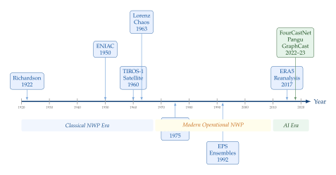
Richardson's Human Computer (1922). The first attempt at numerical weather prediction was made by Lewis Fry Richardson, a British mathematician and pacifist, during his service as an ambulance driver in World War I. Over the years 1916–1918, working in farmhouses and barns in northern France during artillery barrages (he famously stored his calculations in a haystack), Richardson solved by hand a discretised version of the primitive equations governing atmospheric motion.
His 1922 monograph, Weather Prediction by Numerical Process, presented a six-hour forecast for a single location over central Europe. The result was catastrophically wrong: he predicted a surface pressure change of 145 hPa when the actual change was near zero. The error, Richardson later understood, arose from using initial data with unbalanced divergence fields that excited spurious high-frequency gravity waves-a numerical stability problem that would not be solved until the work of Charney and Eliassen in the 1950s.
Nevertheless, Richardson's conceptual framework was entirely correct. He imagined a “forecast factory” of 64,000 human computers working in parallel, each solving the equations for one grid cell, coordinated by a conductor at the centre like a grand orchestra. This vision anticipated both the structure of parallel computing and the ensemble prediction paradigm by more than half a century.
Historical Note.
ENIAC and the First Successful NWP (1950). In 1950, a team led by Jule Charney, with participation by John von Neumann, used the ENIAC computer at the Aberdeen Proving Ground in Maryland to produce the first successful numerical weather forecast. The computation used a simplified version of the atmospheric equations (the barotropic vorticity equation, a single-layer model) on a coarse mesh (a grid of about 270 points at roughly 736 km spacing) covering North America. The actual computation took 24 hours of machine time to forecast 24 hours of atmospheric evolution-a “forecast” that was useful only in retrospect. But the results, published in 1950, showed skill comparable to subjective forecasters and demonstrated unambiguously that numerical methods could predict the large-scale flow.
Von Neumann, who had championed the weather prediction programme as a demonstration of the potential of electronic computing, reportedly called it “the most complex calculation ever attempted.” The ENIAC's computational throughput was approximately 5,000 floating-point operations per second. A modern desktop GPU performs such operations per second-seven orders of magnitude more-yet operational NWP still consumes a significant fraction of the world's most powerful supercomputer capacity.
Historical Note.
The Age of Satellites, Ensembles, and Data Assimilation (1960s–2010s). The launch of TIROS-1 in 1960, the first weather satellite, transformed observational coverage, particularly over the data-sparse oceans that cover 71% of Earth's surface. The modern Global Observing System now integrates approximately observations per day, drawn from surface stations, ocean buoys, radiosondes, aircraft, and a constellation of polar-orbiting and geostationary satellites.
The 1990s saw the operational introduction of ensemble prediction systems (EPS) at ECMWF and the US National Centers for Environmental Prediction (NCEP). Rather than running a single deterministic forecast, an EPS runs 20–50 perturbed versions of the model simultaneously, sampling the uncertainty in initial conditions. The spread of the ensemble provides a first-order estimate of forecast uncertainty; when the ensemble is tight, confidence is high; when it fans out, the atmosphere is in a regime of low predictability. The ECMWF Ensemble (ENS), now running at approximately 18 km resolution with 51 members, remains the gold standard against which all new approaches are evaluated.
The timeline of these developments is shown in Figure 1.
Lorenz and the Mathematics of Chaos
In 1963, Edward Lorenz published what would become one of the most cited papers in all of science: Deterministic Nonperiodic Flow, in the Journal of the Atmospheric Sciences. Working on a simplified model of atmospheric convection, Lorenz stumbled upon behaviour that would transform our understanding of determinism.
His model consisted of three coupled ordinary differential equations: (Lorenz1) with canonical parameters , , . These equations exhibit what Lorenz called sensitive dependence on initial conditions: two trajectories starting arbitrarily close together diverge exponentially, with a characteristic Lyapunov exponent per nondimensional time unit of the system.
Definition 1 (Lyapunov Exponent).
Let be a trajectory of a dynamical system and let be an infinitesimal perturbation evolving under the linearised flow. The maximal Lyapunov exponent is: (Lyapunov) When , the system is chaotic: nearby trajectories diverge exponentially. For the Lorenz system, ; for the real atmosphere, the leading Lyapunov exponent corresponds to an error-doubling time of approximately 1.5–2.5 days.
The practical implication for weather forecasting is profound. If the leading Lyapunov exponent of the atmosphere corresponds to an error-doubling time of two days, and if we cannot measure initial conditions with infinite precision, then beyond some finite horizon the forecast error will be comparable to the climatological variance-at which point the forecast has no skill.
Theorem 1 (Predictability Limit).
Let denote the climatological variance of a forecast variable, and let denote the analysis error variance (the uncertainty in the initial condition). Under the assumption of linear error growth with Lyapunov exponent , the forecast error variance at lead time satisfies: (Error Growth) The predictability horizon is defined as the lead time at which forecast error equals climatological variance: (Horizon) Empirically, weeks for large-scale atmospheric variables.
Remark 1 (Beyond the Predictability Horizon).
The two-week predictability limit applies to the deterministic atmosphere: the expectation of the forecast. Probabilistic quantities-the distribution of possible outcomes-remain informative at longer lead times. Climate models, for instance, project changes in the statistics of extremes decades hence, not by predicting individual events, but by estimating shifts in the underlying probability distribution. This distinction is fundamental and motivates much of the chapter.
Formal Definitions: The Atmospheric State and Forecast Operator
We now formalise the mathematical framework for weather prediction, establishing notation that will be used throughout the chapter.
Definition 2 (Atmospheric State Vector).
The atmospheric state at time is represented by a vector , where is the state space. For a global forecast model at horizontal resolution with pressure levels, the state vector typically includes: (State) where are horizontal grid indices, is the pressure level index, is temperature, are horizontal wind components, is specific humidity, is vertical velocity, and is geopotential. The dimensionality of the ERA5 reanalysis grid (used to train most current ML weather models) is approximately at the operational resolution with 37 levels (a grid over 37 levels and roughly six upper-air fields plus surface fields); at a coarser resolution it is about .
Definition 3 (Forecast Operator).
A deterministic forecast operator with lead time is a mapping such that: (Deterministic OP) In classical NWP, is implemented by numerically integrating the primitive equations of atmospheric motion using finite difference, finite element, or spectral discretisation. In machine learning weather prediction (MLWP), is approximated by a neural network with parameters learned from reanalysis data.
Definition 4 (Probabilistic Forecast Operator).
A probabilistic forecast operator is a mapping from the current state to a probability distribution over future states: (PROB OP) where maps states to distributions over . The ideal probabilistic forecast is the true conditional distribution of atmospheric states, which reflects both initial-condition uncertainty (arising from imperfect observations and data assimilation) and model uncertainty (arising from approximations in the governing equations and their discretisation). Generative models are, at their core, parametric approximations to .
Remark 2 (Autoregressive Rollout).
For forecast horizons longer than , a common approach is autoregressive rollout: apply the operator (or sample from ) repeatedly, using each predicted state as the next input: (Rollout) In the probabilistic setting, autoregressive rollout produces a trajectory distribution; errors can compound over rollout steps, which is one of the central practical challenges in MLWP.
The Operational Bottleneck: Compute Cost and the NWP Scaling Problem
Modern operational NWP represents one of the most computationally demanding regular tasks in all of science. ECMWF's Integrated Forecasting System (IFS), which produces the world's leading medium-range global forecasts, runs on a dedicated supercomputer cluster with a peak performance of approximately floating-point operations per second (100 petaFLOPS). A single ten-day global forecast at km resolution requires roughly floating-point operations-approximately times more than a single forward pass through a large language model.
The computational cost of NWP scales approximately as: (NWP COST) where is the horizontal grid resolution, is the number of vertical levels, and is the number of time steps. Halving the horizontal grid spacing increases cost by a factor of (two factors in horizontal resolution, one in time step required for numerical stability by the Courant–Friedrichs–Lewy condition).
Proposition 1 (Cost of NWP Resolution Increase).
Let denote the horizontal grid spacing of a global NWP model. Under typical operational configurations with a CFL-constrained time step , the computational cost of a fixed lead-time forecast scales as: (COST Scaling) where is the number of spatial dimensions. For (global horizontal grid with fixed vertical levels), . Moving from km to km global resolution therefore increases cost by a factor of . Kilometre-scale global NWP is projected to become operationally feasible by the early 2030s on exascale hardware, but will require times the computational resources of current systems.
Key Idea.
Weather Forecasting as Sampling from a Chaotic Distribution Weather forecasting is fundamentally a problem of sampling from a chaotic conditional probability distribution. Given the current atmospheric state , the true forecast is not a single predicted state but the entire conditional distribution . This distribution is:
High-dimensional: for operational-resolution () grids.
Non-Gaussian: especially for precipitation and extreme variables.
Strongly multimodal: the atmosphere can follow qualitatively different trajectories (e.g., blocking high vs. progressive westerlies) with comparable probability.
Physically constrained: samples must approximately satisfy conservation laws (mass, energy, momentum) and balance conditions.
Generative models-diffusion models, normalising flows, GANs, and their modern variants-are precisely the class of methods designed to learn and sample from distributions of this kind.
The Quiet Revolution: Skill Improvement in Traditional NWP
The sixty-year history of operational NWP reveals a remarkable and sustained trend in forecast skill: roughly one day of useful forecast range gained per decade. This improvement is most clearly measured by the anomaly correlation coefficient (ACC) of the 500 hPa geopotential height field-a standard metric that compares the forecast anomaly (deviation from climatology) with the verifying analysis. An ACC above 0.6 is conventionally considered the threshold of useful skill.
In 1980, ECMWF forecasts crossed the ACC, threshold at approximately 5 days lead time. By 2020, the threshold had extended to approximately 8.5 days. This represents a gain of 3.5 days over four decades. Equivalently, the quality of today's seven-day forecast is roughly comparable to the quality of a three-day forecast in 1980. The improvement reflects advances in:
Data assimilation: Moving from optimal interpolation to four-dimensional variational assimilation (4D-Var), which optimally blends observations with model trajectories over a 6–12 hour assimilation window.
Model resolution: From 150 km in 1979 to 9 km in 2023, enabling better representation of orographic and mesoscale processes.
Physical parameterisations: Improved schemes for convection, boundary layer turbulence, radiation, and cloud microphysics.
Observations: The global observing network has grown from surface stations in 1980 to observations per day from the current satellite constellation.
Insight.
The history of NWP skill improvement suggests diminishing returns in the traditional paradigm: each additional day of forecast range costs approximately twice the compute of the previous. Meanwhile, the recent AI-based models (FourCastNet, Pangu-Weather, GraphCast, FengWu, Aardvark, and others) achieve comparable or superior skill to IFS at a computational cost four to six orders of magnitude lower per inference. This is not an incremental improvement; it represents a fundamental change in the cost-skill frontier of weather forecasting.
Exercises for Section The Challenge of Atmospheric Prediction
Exercise 1 (Lyapunov exponent and predictability).
Consider a simple model of atmospheric error growth in which the error satisfies with (corresponding to an error-doubling time of two days).
- (a)
Show that .
- (b)
If the analysis error is of the climatological standard deviation, compute the predictability horizon using Theorem 1.
- (c)
How does change if observations improve and is halved? What does this imply about the practical ceiling of medium-range forecast skill?
Exercise 2 (NWP computational cost).
Using the scaling relation of Proposition 1:
- (a)
Estimate the cost ratio of a km global forecast relative to the current operational ECMWF system at km, assuming the same number of vertical levels and lead time.
- (b)
If a km global NWP system requires 10,000 node-hours per forecast cycle, and if node-hours cost $0.50 on a cloud HPC facility, estimate the annual cost of running 50-member ensemble forecasts every 12 hours.
- (c)
Compare this to the estimated inference cost of a state-of-the-art ML weather model, which can produce a 10-day global forecast in under 60 seconds on a single GPU. What is the approximate cost ratio?
Exercise 3 (Atmospheric state dimensionality).
The ERA5 reanalysis provides the following variables on a latitude-longitude grid ( points) at 37 pressure levels: temperature (), zonal wind (), meridional wind (), specific humidity (), and geopotential (). Additionally, four single-level variables are included: mean sea-level pressure, 2-metre temperature, and 10-metre wind components.
- (a)
Compute the total number of degrees of freedom in the ERA5 state representation.
- (b)
Compare to the number of parameters in a large language model (e.g., GPT-3 with 175 billion parameters). What does this suggest about the relative difficulty of the weather forecasting and language modelling problems?
- (c)
Most ML weather models operate at resolution (roughly grid points) or . How does the dimensionality change, and what are the implications for model capacity requirements?
Why Generative AI for Weather?
The previous section established that weather forecasting is, at its mathematical core, a problem of learning and sampling from a high-dimensional conditional probability distribution. It also established that the classical NWP paradigm, while enormously successful, faces a cost wall: operational ensemble forecasting with 50 members at high resolution consumes resources available only to the largest national meteorological centres. In this section we examine more precisely why generative models offer a compelling solution to these challenges, and how they relate to the broader taxonomy of machine learning approaches to weather prediction.
The Three Pillars: Cost, Ensembles, and Extremes
The case for generative models in weather prediction rests on three mutually reinforcing pillars.
Pillar 1: Computational Cost
As established in Proposition 1, the cost of a single NWP forecast is enormous, and the cost of an ensemble forecast is this number multiplied by the ensemble size. A 50-member ensemble at km global resolution, run for a 10-day lead time, requires on the order of floating-point operations-enough to occupy the ECMWF supercomputer for several hours. Only a handful of national centres worldwide have the resources to run such systems operationally.
By contrast, a trained generative model produces ensemble members by forward sampling, which requires a single forward pass through a neural network (or, for diffusion models, a sequence of –100 such passes). The total inference cost is: (GEN COST) where is the cost of a single neural network forward pass. For a model like GenCast or SEEDS, this amounts to roughly operations per 50-member ensemble-seven orders of magnitude less than the NWP equivalent.
Pillar 2: Ensemble Generation and Calibration
Operational ensemble prediction systems generate spread by perturbing initial conditions (using singular vectors or ensemble Kalman filter perturbations) and sometimes by stochastic model perturbations. These perturbations are designed to sample the leading error modes of the system, but they are necessarily limited in their ability to represent the full uncertainty distribution.
A well-trained generative model, by contrast, learns the full conditional distribution from data. If the training data is sufficiently rich and diverse, the model can in principle capture uncertainty sources that are difficult to parameterise explicitly in physical models: mesoscale convective organisation, land-surface feedback uncertainty, orographic precipitation spread, and more. This offers the prospect of better-calibrated ensembles-ensembles whose spread more faithfully represents the true forecast uncertainty.
Definition 5 (Calibration).
A probabilistic forecast is calibrated (or reliable) if the stated probabilities match observed frequencies. Formally, for any event and stated probability : (Calibration) In practice, calibration is assessed via rank histograms (Talagrand diagrams) for ensemble systems, or reliability diagrams for probabilistic forecasts. A perfectly calibrated 50-member ensemble should have each of the 50 members verified against the true observation equally often on average; a flat rank histogram indicates calibration.
Generative models offer a systematic path to calibration improvement through post-processing: rather than running the expensive NWP ensemble and then applying bias correction, one can train a conditional generative model to map a deterministic (or low-resolution) NWP forecast directly to a calibrated ensemble distribution. This is the ensemble emulation paradigm explored in GenCast, NowcastNet, and similar systems.
Pillar 3: Extreme Events
Extreme weather events-heat waves, atmospheric rivers, tropical cyclones, flash floods-are precisely the events for which forecast skill matters most, both in terms of economic impact and loss of life. They are also, almost by definition, the hardest to forecast.
Traditional ML weather models trained with mean squared error (MSE) loss face a fundamental problem with extremes: MSE minimisation encourages predictions that are close to the conditional mean, which for multimodal distributions is not a typical sample. A model predicting whether a storm will track north or south of a coastal city, each with 50% probability, should predict one or the other-not an average track that lies in the middle of the coast and is unlikely to verify. MSE-optimal forecasts are necessarily smooth, tending to regress toward climatology for uncertain events. This is the blurring problem.
Caution.
The blurring problem in deterministic ML weather models is not merely a cosmetic issue. A 24-hour precipitation forecast that smears a 100 mm/day convective event over a 1,000 km region has an RMSE comparable to the unsmeared forecast but provides no useful information for flash flood warning. Generative models address this problem structurally by learning to sample sharp, physically plausible realisations rather than predicting blurred averages.
Generative models, by learning to sample from the full conditional distribution, can in principle produce sharp forecasts of extreme events. A diffusion model conditioned on a predicted atmospheric state can generate individual sample trajectories that include coherent, physically realistic extreme events, even if those events appear in only a fraction of the ensemble members. The probability of the event is estimated from the ensemble frequency.
Deterministic MLWP: Limitations and Where Generative Models Help
The first generation of modern ML weather models-FourCastNet (2022), Pangu-Weather (2023), GraphCast (2023)-are deterministic systems that directly predict the atmospheric state at the next time step. They have demonstrated remarkable skill, matching or exceeding the ECMWF IFS for many variables at 7–10 day lead times while running at a fraction of the computational cost.
However, their fundamental architecture-a neural network trained to minimise MSE between predicted and verifying states-imposes a systematic bias: the regression to the mean problem. Consider the formal decomposition: (MSE Solution) where the equality in holds because MSE minimisation yields the conditional expectation. For multimodal distributions -which are common in the atmosphere, especially at longer lead times when the flow can bifurcate into qualitatively different regimes-the conditional mean is not a typical sample. It lies between the modes, in a region of low probability density.
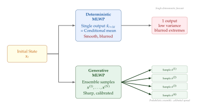
Figure 2 illustrates the architectural difference between deterministic and generative MLWP. The key structural insight is that the conditional mean-the optimal deterministic forecast under MSE loss-is not the same as the most likely forecast, and for multimodal distributions it may lie in a region of essentially zero probability.
Example 1 (Blurring in Precipitation Forecasts).
Consider the 6-hour accumulated precipitation field over the United Kingdom. The true distribution is highly multimodal: convective cells may form in the Thames valley or in Wales or both, depending on subtle mesoscale features. A deterministic model predicts the conditional mean, which spreads the precipitation evenly across both potential locations at half the intensity. This “drizzle everywhere” artefact is a well-documented failure mode of MSE-trained models. Operationally, precipitation skill scores such as the fractions skill score (FSS) and equitable threat score (ETS) specifically penalise spatial displacement errors, making this artefact visible in standard verification.
A generative model, by contrast, draws individual sample realisations that place the precipitation coherently in one location or the other, each with intensity close to the true event. The ensemble mean may still be blurred, but any individual sample is physically sharp-which is what matters for flash flood warnings.
Ensemble Prediction Systems and the Cost of NWP Ensembles
The state-of-the-art in operational probabilistic forecasting is the ensemble prediction system (EPS). The flagship systems are:
ECMWF ENS: 51 members (1 control + 50 perturbed) at km resolution, 15-day lead time. Initial perturbations generated by singular vectors and ensemble data assimilation; model uncertainty represented by stochastic parameterisation schemes.
NOAA GEFS (Global Ensemble Forecast System): 31 members at km, 16-day lead time; being upgraded to higher resolution under the Next Generation Global Prediction System (NGGPS) programme.
UK Met Office MOGREPS-G: 18 members at km; uses the ensemble transform Kalman filter (ETKF) for perturbation generation.
Multi-model ensembles: The THORPEX Interactive Grand Global Ensemble (TIGGE) archive collects outputs from all major operational EPS systems, enabling multi-model ensemble combinations that typically outperform any individual system.
The computational cost of running 50 ensemble members is, approximately, 50 times the cost of a single deterministic forecast. For the ECMWF system in 2023, this amounts to approximately 30 megawatt-hours of electricity per day-comparable to the annual electricity consumption of 3,000 European households. The energy and financial cost of ensemble NWP is a fundamental barrier to democratising access to probabilistic weather services: most national meteorological services in developing countries cannot afford to run their own ensemble systems and rely on the ECMWF or NOAA outputs.
Insight.
Generative models as ensemble emulators could democratise probabilistic forecasting. A country with a single GPU server could run a trained generative model to produce 100-member ensembles conditioned on the publicly available ECMWF deterministic forecast, achieving calibrated probability estimates at a cost thousands of times lower than running a physical ensemble. This is not hypothetical: the SEEDS model (Stockdale et al., 2024) and the EPS emulator of Price et al. (2023) have demonstrated this approach operationally.
Formal Framework: Weather Forecasting as Conditional Generative Modelling
We now place weather forecasting squarely within the conditional generative modelling framework developed in earlier chapters of this book.
Definition 6 (Weather Forecast as Conditional Distribution).
Given the current atmospheric state , the ideal probabilistic weather forecast at lead time is the conditional distribution: (COND DIST) which represents the probability that the atmosphere will be in state at time given that it is in state at time . This distribution encodes both:
Initial-condition uncertainty: arising from imperfect observations and data assimilation, the true atmospheric state at time is uncertain; marginalises over this uncertainty.
Intrinsic atmospheric uncertainty: arising from the chaotic dynamics of the atmosphere, even a perfectly known initial state leads to a spread of possible outcomes at long lead times.
A generative model is a parametric approximation: (GEN Model)
This framework immediately suggests the applicability of the main generative model families covered in this book:
Diffusion models (Chapter 19): Learn by training a denoising score network . Sampling proceeds via Langevin dynamics or DDIM. Key models: GenCast, CorrDiff, EarthFormer-Diffusion.
Normalising flows (Chapter 18): Model as a pushforward of a standard Gaussian through an invertible map . Exact likelihoods enable principled calibration assessment. Key models: RainFall (Gong et al., 2023), NF-based post-processing (Groenke et al., 2022).
Variational Autoencoders (Chapter 15): A latent-variable model for atmospheric state that enables compressed representations and fast sampling. Key models: WeatherVAE, GenWP.
GANs (Chapter 9): Generative Adversarial Networks for downscaling and super-resolution of weather fields. Key models: DeepSD (Stengel et al., 2020), DeepMind's downscaling GAN, ESRGAN-based approaches.
A Taxonomy of ML Weather Prediction Approaches
The landscape of ML weather prediction has grown dramatically since 2020. To navigate it, we introduce a systematic taxonomy along four axes: (1) model type (deterministic vs. generative), (2) spatial scope (global vs. regional/limited-area), (3) temporal architecture (autoregressive vs. direct multi-step), and (4) target variable (full atmosphere vs. single-variable).
Table 1 provides a structured overview of the most influential models along these axes.
| Model | Type | Scope | Temporal | Res. | Key Feature |
| Deterministic Global Models | |||||
| FourCastNet | Det. | Global | AR | Spherical FNO | |
| Pangu-Weather | Det. | Global | Direct | 3D Earth transformer | |
| GraphCast | Det. | Global | AR | Graph neural network | |
| FengWu | Det. | Global | AR | Cross-modal fusion | |
| Aardvark | Det. | Global | AR | Sparse observations in | |
| Generative Global Models | |||||
| GenCast | Diffusion | Global | AR | Calibrated ensembles | |
| SEEDS | Diffusion | Global | Emulator | EPS emulation | |
| PreDiff | Diffusion | Regional | AR | km | Nowcasting |
| CorrDiff | Diffusion | Regional | AR | km | Downscaling |
| EarthFormer | Diff+Attn | Regional | AR | Earth attention | |
| Nowcasting and Short-Range | |||||
| NowcastNet | GAN | Regional | Direct | km | Extrapolation |
| Skilful Prec. | GAN | Regional | Direct | km | DeepMind GAN |
| DGM-R | NF | Regional | AR | Radar nowcast | |
| Downscaling / Super-Resolution | |||||
| DeepSD | GAN | Regional | Direct | km | Statistical SD |
| CorrDiff | Diffusion | Regional | Direct | km | Score-based SD |
| GenRain | Flow | Regional | Direct | km | Probabilistic |
Chapter Roadmap and Dependencies
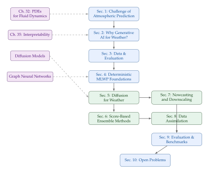
This chapter is structured to develop the material from foundational principles through state-of-the-art models and open problems. Figure 3 shows the dependency structure between sections.
Remark 3 (Connections to Other Chapters).
This chapter connects to several other chapters in the book:
Chapter 35 (PDEs for Fluid Dynamics): The primitive equations of atmospheric motion are a system of PDEs; understanding their structure (balanced flow, the primitive equations, quasi-geostrophic theory) provides crucial physical intuition for why certain ML architectures succeed and others fail.
Chapter 38 (Interpretability): Understanding what a weather model has learned-which atmospheric patterns it attends to, which teleconnections it has discovered, whether its representations align with physical modes like ENSO or the North Atlantic Oscillation-is an active research frontier.
Chapter 19 (Diffusion Models): The core generative modelling machinery of this chapter is the score-based diffusion framework. Readers unfamiliar with denoising score matching and the SDE formulation of diffusion should review that chapter before proceeding to Section 5 of the present chapter.
Exercises for Section Why Generative AI for Weather?
Exercise 4 (The regression-to-mean problem).
Consider a bimodal conditional distribution: (Bimodal) where and are two distinct modes with and is small (each mode is tight).
- (a)
Show that the MSE-optimal forecast is .
- (b)
Compute the probability density of the MSE-optimal forecast under as a function of . For what value of does the MSE forecast lie in a region of near-zero density?
- (c)
Define the sharpness of a single forecast under distribution as . Show that a randomly sampled forecast has higher expected sharpness than the MSE-optimal forecast when .
Exercise 5 (Calibration of ensemble forecasts).
An ensemble forecast system produces members. Over a verification archive of forecast-observation pairs, the rank of the observation within the sorted ensemble (rank 1 = observation below all members, rank = observation above all members) has the following histogram:
| Rank | 1 | 2 | 3 | 4 | 5 | 6 | 7 | 8 | 9 | 10 | 11 |
| Count | 152 | 89 | 82 | 88 | 91 | 89 | 87 | 85 | 82 | 86 | 169 |
- (a)
Under the null hypothesis of a perfectly calibrated ensemble, what count would you expect in each rank bin?
- (b)
The U-shaped histogram (high counts at ranks 1 and 11) indicates a specific type of calibration failure. Identify the failure mode and suggest two possible causes.
- (c)
Compute a chi-squared statistic for the deviation from uniformity and determine whether the miscalibration is statistically significant at the level.
Exercise 6 (Ensemble size and sampling error).
A 50-member ensemble is used to estimate the probability that 24-hour precipitation at a point exceeds 50 mm. Suppose the true probability is .
- (a)
Model the number of ensemble members exceeding the threshold as . Compute the standard deviation of the estimated probability where is the count.
- (b)
What ensemble size would be required to estimate (a 1-in-100 event) with a coefficient of variation (standard deviation divided by mean) below 20%?
- (c)
Comment on the practical implications for using NWP ensembles vs. generative model ensembles for estimating rare event probabilities. A generative model can produce thousands of samples at marginal cost; how does this change the analysis in part (b)?
The Governing Equations of the Atmosphere
“The atmosphere is a nonlinear fluid on a rotating sphere, forced by solar radiation and interacting with the ocean, land, and biosphere. Its equations are simple to write, impossible to solve exactly, and extraordinarily difficult to approximate well.” - Edward N. Lorenz (paraphrased)
Weather prediction is, at its mathematical core, an initial value problem for a system of nonlinear partial differential equations. The atmosphere is a thin shell of gas-roughly 100,km thick over a planet of radius ,km-set in rotation at one revolution per day, heated unevenly from below by sunlight, and stirred by the irregular topography of continents and mountain ranges. Despite this complexity, the fundamental physical laws governing atmospheric motion are well known. They form the primitive equations, a closed system of PDEs derived from Newtonian mechanics, thermodynamics, and the ideal gas law.
In this section we derive and discuss these equations in detail, connect them to the general Navier–Stokes framework introduced in Chapter 35 (Section The Navier--Stokes equations: beauty and terror), and explain why, despite being fully known, they resist exact solution and force us toward numerical approximation.
Coordinate systems and notation
The Earth's atmosphere is most naturally described in spherical coordinates , where is longitude, is latitude, and is the radial distance from Earth's centre with mean radius and height above the surface . In practice, NWP models use a hybrid pressure–terrain-following coordinate or , which simplifies the treatment of the lower boundary.
We denote the three-dimensional velocity field as , where is the zonal (east–west) component, is the meridional (north–south) component, and is the vertical velocity. For notational simplicity in the following subsections, we work in local Cartesian coordinates on the sphere (the tangent plane approximation), which is exact in the limit of small horizontal scales and standard in textbook derivations.
The material derivative (Lagrangian rate of change following a fluid parcel) is (Material) where denotes the three-dimensional gradient operator. The distinction between Eulerian ( at a fixed point) and Lagrangian ( following a parcel) perspectives is essential throughout atmospheric dynamics.
The momentum equation: Navier–Stokes on a rotating sphere
Newton's second law for a fluid parcel in an inertial frame gives the Navier–Stokes equations (Chapter 35, Section The Navier--Stokes equations: beauty and terror). Transforming to a reference frame rotating with the Earth at angular velocity (where and points toward the North Pole) introduces two pseudo-forces: the Coriolis acceleration and the centrifugal acceleration . The centrifugal term is absorbed into a modified gravitational acceleration (pointing effectively downward, of magnitude ). The result is the atmospheric momentum equation: (Momentum) where is pressure, is air density, is effective gravity, and represents frictional and turbulent drag forces (which act primarily in the planetary boundary layer and through parameterised gravity-wave drag).
The term is the Coriolis acceleration. In local coordinates at latitude , defining the Coriolis parameter , the horizontal momentum equations take the familiar form: (Momentum U) At mid-latitudes (), , so the Coriolis force is significant for synoptic-scale motions (cyclones, anticyclones) but negligible at small scales (thunderstorms, boundary layer turbulence).
Remark 4 (Connection to Chapter 35).
Equation is the Navier–Stokes momentum equation (Chapter 35, Eq. (Momentum)) with two modifications: (i) the compressible form with variable density , and (ii) the Coriolis pseudo-force arising from the rotating reference frame. The atmosphere is a compressible, stratified, rotating fluid, making it significantly more complex than the canonical incompressible setting studied in Chapter 35.
The continuity equation: conservation of mass
Mass conservation for a compressible fluid yields the continuity equation: (Continuity) or equivalently, using the material derivative: (Continuity Lagrange) This states that the density of an air parcel changes only through divergence of the velocity field. A convergent flow () compresses air parcels and increases their density.
In the Boussinesq approximation, valid for small density variations (useful for ocean dynamics but less so for the full atmosphere), is treated as constant and one recovers the incompressibility condition . The full atmosphere requires the compressible form.
The thermodynamic energy equation
The first law of thermodynamics applied to a fluid parcel gives the thermodynamic energy equation, governing temperature evolution: (Thermo) where is temperature, is the specific heat at constant pressure, and is the diabatic heating rate per unit mass (units ). The diabatic heating encompasses:
Radiative heating: absorption of solar shortwave radiation and emission/absorption of terrestrial longwave radiation;
Latent heat release: phase changes of water (condensation releasing heat, evaporation absorbing heat);
Sensible heat fluxes: exchange of heat between the atmosphere and the underlying surface;
Diffusion and turbulent mixing: small-scale transport of heat by unresolved eddies.
When , the process is adiabatic: temperature changes only through compression and expansion as the parcel moves vertically in the pressure gradient.
Using the ideal gas law (Section The equation of state: the ideal gas law) to eliminate , the thermodynamic equation can be rewritten in terms of potential temperature , where is a reference pressure and is the gas constant for dry air: (Pottemp) Potential temperature is conserved following an adiabatic parcel and is the natural prognostic variable for the thermodynamic equation in NWP models.
The moisture equation
Water in the atmosphere exists in three phases (vapour, liquid, ice) and plays a crucial role in weather through cloud formation, precipitation, and latent heat release. The prognostic equation for specific humidity (mass of water vapour per unit mass of moist air, ) is: (Moisture) where is the net source/sink term including:
condensation and evaporation from cloud microphysics;
precipitation (removing liquid water from the column);
surface evaporation (adding moisture at the lower boundary);
turbulent transport within the boundary layer.
In full models, separate equations are carried for cloud liquid water , cloud ice , rain , and snow , each with its own source/sink parameterisation. The latent heat release when water vapour condenses directly feeds back into the thermodynamic equation via , where is the latent heat of vaporisation.
The equation of state: the ideal gas law
Air behaves to excellent approximation as an ideal gas. The equation of state closes the system by relating pressure, density, and temperature: (EOS) where is the gas constant for dry air and is the virtual temperature, which accounts for the lower molecular weight of water vapour (). For dry air (), and the familiar ideal gas law applies.
The primitive equations as a formal system
We can now state the complete governing system.
Definition 7 (Primitive equations).
The primitive equations of the atmosphere are the system of PDEs governing the evolution of wind , temperature (or potential temperature ), specific humidity , and pressure (or density ): (PRIM MOM) This is a system of seven scalar PDEs (three momentum components, one continuity, one thermodynamic, one moisture, one algebraic state equation) in seven unknowns as functions of , closed by prescribing the diabatic terms , , and through parameterisation schemes.
Conservation properties
The primitive equations conserve fundamental physical quantities in the absence of diabatic forcing and friction. This is a cornerstone of both the theoretical analysis and the numerical implementation of atmospheric models.
Theorem 2 (Energy and mass conservation for the primitive equations).
Consider the primitive equations – on a domain (the atmospheric volume) with no-normal-flow boundary conditions and , , . Then:
Total mass conservation: (MASS CONS)
Total energy conservation: The sum of kinetic energy , internal energy , and potential energy is conserved: (Energy CONS) where , ( specific heat at constant volume), and .
Sketch.
Mass conservation follows directly from the continuity equation by integrating over and applying the divergence theorem with no-normal-flow boundary conditions. Energy conservation follows from taking the scalar product of with the momentum equation to obtain the kinetic energy budget, adding the thermodynamic equation (rewritten as an internal energy equation using ), and adding the gravitational potential energy equation . The pressure work terms cancel through the continuity equation, yielding .
Remark 5.
Preserving these conservation laws discretely (i.e., in the numerical approximation) is a major constraint on the design of NWP models. A model that fails to conserve total mass will develop a spurious mass drift over long integrations. Mimetic discretisations and geometric integrators (Section Discretisation strategies) are designed precisely to inherit the continuous conservation properties.
The hydrostatic approximation
The atmosphere's extreme aspect ratio-horizontal scales of thousands of kilometres versus vertical scales of tens of kilometres-implies that vertical accelerations are negligibly small compared to the dominant balance between gravity and the vertical pressure gradient. This yields the hydrostatic approximation, obtained by setting in Eq. : (Hydrostatic) This single equation replaces the vertical momentum equation, reducing the prognostic system by one equation. Hydrostatic models are appropriate for horizontal scales larger than ,km; at smaller scales (cloud-resolving models, large-eddy simulations), the full non-hydrostatic equations are required.
Combined with the shallow atmosphere approximation-treating the atmosphere as a thin shell so that throughout-one arrives at the equations used in virtually all global operational NWP models. Departures from the shallow atmosphere assumption become non-negligible only at very high altitudes.
Boundary conditions
The primitive equations require boundary conditions at two surfaces:
Lower boundary (Earth's surface).
At the surface (terrain height), the kinematic boundary condition requires that no air passes through the surface: (BC Lower) For a stationary surface (), this says that vertical velocity equals the slope of the terrain times the horizontal wind-air is deflected over mountains. Thermodynamic and moisture boundary conditions prescribe surface fluxes of heat and water vapour, computed from land-surface and ocean models.
Upper boundary (top of atmosphere).
At the model top , the pressure is set to a small value (–, corresponding to the stratosphere or mesosphere). A sponge layer absorbs spurious wave reflections near the model top.
Atmospheric structure
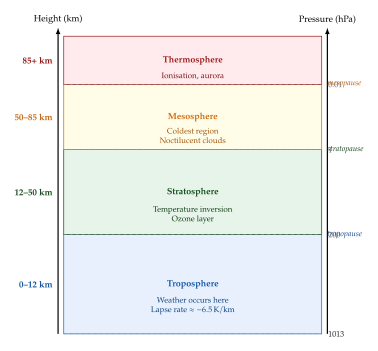
The primitive equations govern motion throughout the atmosphere, but different vertical layers have distinct dynamical regimes. Figure 4 shows the standard atmospheric stratification.
Why direct numerical simulation is impossible
Remark 6 (The scale problem: why DNS of the atmosphere is impossible).
The atmosphere contains approximately molecules. A direct numerical simulation (DNS) resolving every molecular interaction would require a computational mesh with grid points. Even if each grid point required only one byte of storage, this would demand ,bytes-roughly times more than all the data ever created by humanity.
More concretely, atmospheric turbulence spans scales from the molecular mean free path (,m) to synoptic systems (,m), a range of in length. DNS of Navier–Stokes at the atmospheric Reynolds number would require a three-dimensional grid of points per atmospheric layer (Kolmogorov scaling). A global DNS is utterly beyond any conceivable computing technology.
This fundamental impossibility is the reason why parameterisation, numerical approximation, and machine learning are not merely convenient, but necessary, for any practical atmospheric simulation.
Parameterisation of sub-grid processes
Because a global NWP model operates on a grid with typical spacing –, all physical processes occurring at smaller scales must be parameterised: represented through equations relating their aggregate effect to the resolved grid-scale variables. The main parameterisation schemes in a state-of-the-art NWP model are:
Radiation.
Atmospheric radiation involves absorption and emission across millions of spectral lines of , , , and other gases. Full line-by-line calculations are computationally prohibitive for NWP; instead, two-stream approximations or correlated- methods provide accurate broadband fluxes at manageable cost. Radiation parameterisation is among the most computationally expensive components of a GCM.
Convection.
Thunderstorms and moist convection organise at scales of 1–10,km, far below the grid scale of global models. Mass flux or entraining plume schemes represent the effects of deep and shallow convection on the column temperature and moisture profiles. Errors in convective parameterisation are among the leading sources of forecast error in the tropics.
Cloud microphysics.
The formation and growth of cloud droplets, ice crystals, and precipitation particles involves processes from nanometre to millimetre scales. Bulk microphysics schemes represent clouds through moment equations for the distribution of hydrometeor sizes; spectral bin schemes are more accurate but far more expensive.
Planetary boundary layer.
The lowest 1–2,km of the atmosphere is the planetary boundary layer (PBL), where turbulent eddies transfer momentum, heat, and moisture between the surface and the free atmosphere. PBL schemes typically use mixing-length or turbulence kinetic energy (TKE) closures to represent this transport.
Gravity wave drag.
Sub-grid-scale orographic and convective gravity waves transport momentum vertically, decelerating the large-scale flow when they break. This drag is critical for the correct simulation of the stratospheric circulation and must be parameterised in global models.
The parameterisation problem is not merely a technical inconvenience-it is a fundamental scientific challenge. Errors in parameterisation account for a large fraction of model bias and uncertainty, particularly in climate projections. Machine learning approaches to learned parameterisation (replacing hand-tuned schemes with data-driven approximations) are an active frontier, discussed in later sections.
Historical background: from Richardson to ENIAC
The idea that weather could be predicted by solving the equations of fluid motion numerically dates to Lewis Fry Richardson (1881–1953). In his landmark 1922 book Weather Prediction by Numerical Process, Richardson described in extraordinary detail a scheme for solving the primitive equations on a grid, using a network of 64,000 human computers working in parallel in a vast “forecast factory”. His own attempt at a 6-hour forecast for a point in central Europe-carried out by hand during World War I-took approximately six weeks to compute and produced a catastrophically wrong answer (a pressure change of 145,hPa, when the observed change was near zero) due to an inadequate initialisation procedure.
Richardson's vision proved prophetic. The missing ingredient was data assimilation: a method for initialising the model state consistently with the underlying equations. Without it, the initial conditions contain fast-moving acoustic and gravity waves that swamp the slower weather-bearing Rossby waves, causing the forecast to explode.
The breakthrough came in 1950, when Jule Charney, Ragnar Fjortoft, and John von Neumann produced the first successful numerical weather forecast on the ENIAC computer at the Aberdeen Proving Ground in Maryland (the team was based at the Institute for Advanced Study in Princeton). Working with a simplified barotropic vorticity equation (a single-level filter that eliminates the problematic fast waves), they ran 24-hour forecasts for the 500,hPa geopotential height field over North America. The computation took 24 hours of ENIAC time to produce a 24-hour forecast-a ratio of 1:1. Today's operational models run at ratios of order :1 (about seconds of forecast produced per second of wall-clock time), reflecting seven decades of algorithmic and hardware advances.
Remark 7 (Richardson's legacy).
Richardson's forecast factory was not merely a quaint historical curiosity: it was the first explicit description of a massively parallel computation. Von Neumann's decision to use ENIAC for weather prediction-rather than nuclear weapons calculations-was motivated by his belief that atmospheric simulation would drive the development of digital computing. He was right. The history of NWP is inseparable from the history of supercomputing.
Exercises for Section The Governing Equations of the Atmosphere
Exercise 7.
The Coriolis parameter at the equator is and increases to at the poles.
At latitude N, compute the Coriolis parameter and the inertial period (time for a fluid parcel to complete one inertial oscillation).
A synoptic-scale cyclone has horizontal winds of and a radius of . Compute the Rossby number . Is the Coriolis force important for this system?
For a thunderstorm with and , compute . Can we neglect rotation for thunderstorms?
Exercise 8.
Starting from the ideal gas law and the hydrostatic balance , derive the hypsometric equation relating the thickness of an atmospheric layer to its mean temperature: where is the mean temperature of the layer and are the pressures at the bottom and top of the layer.
The – layer has a mean temperature of C in winter and C in summer. Compute the thickness difference between the two seasons. (This thickness field is a standard diagnostic in operational forecasting.)
Show that for an isothermal atmosphere at temperature , pressure decays exponentially: , where is the scale height. Evaluate for .
Exercise 9.
Consider a global NWP model with horizontal resolution . A deep convective cloud cluster has a typical horizontal scale of and releases latent heat of at a rate of .
Compute the diabatic heating rate in (use ).
This cloud cluster cannot be resolved on the 25,km grid. Explain why simply ignoring it (setting in that grid column) leads to a systematic cold bias in the tropics.
A machine learning parameterisation trained on cloud-resolving model output is used in place of the traditional convective scheme. Describe two potential failure modes: one related to out-of-distribution inputs and one related to physical conservation.
Numerical Weather Prediction Foundations
“NWP is the crown jewel of computational science: a discipline where every factor of two in resolution, every percentage point improvement in initialisation, every better parameterisation scheme translates directly into lives saved and economic losses prevented.” - Attributed to Peter Lynch
The primitive equations of Section The Governing Equations of the Atmosphere form a continuous system of PDEs. To solve them on a computer, we must discretise them: approximate the continuous fields on a finite set of grid points or basis functions, and advance the solution forward in time using a discrete time-stepping scheme. This is the domain of Numerical Weather Prediction (NWP).
NWP is not simply “computational weather”. It is a sophisticated interplay between numerical analysis (stability, accuracy, convergence), dynamical meteorology (wave propagation, balanced flow, geostrophy), computational science (parallelisation, I/O at scale), and data science (assimilation, ensemble generation, probabilistic post-processing). Modern NWP systems represent one of the most complex software engineering endeavours in science-the ECMWF Integrated Forecasting System (IFS) comprises more than two million lines of Fortran code, accumulated over 40 years of continuous development.
Definition 8 (Numerical weather prediction model).
A numerical weather prediction (NWP) model is a computational system that:
approximates the primitive equations – on a discrete grid or spectral basis;
advances the atmospheric state forward in time from prescribed initial conditions;
applies parameterisation schemes for sub-grid physical processes (radiation, convection, microphysics, boundary layer, gravity waves);
produces gridded output fields (wind, temperature, precipitation, etc.) at specified future times.
Discretisation strategies
Three main families of spatial discretisation are used in NWP:
Finite differences
The simplest approach: replace spatial derivatives by algebraic differences between neighbouring grid points. For a uniform grid with spacing , the second-order centred difference for the first derivative is (FD) Finite differences are simple to implement and easily adapted to stretched or variable grids, but achieving high accuracy requires large stencils (many neighbouring points), and formulating them on the sphere requires care near the poles (the “pole problem”).
Spectral methods
In spectral methods, the prognostic variables are expanded in a truncated series of global basis functions. For the sphere, the natural basis is spherical harmonics: (Spectral) where are spherical harmonics of wavenumber and zonal wavenumber , and are spectral coefficients. A triangular truncation at total wavenumber (denoted T) resolves features with a minimum wavelength of approximately where is Earth's radius. ECMWF's operational IFS uses cubic-octahedral grids: TCo1279 () for high-resolution deterministic forecasting (HRES) and TCo639 () for the ensemble.
Spectral methods achieve spectral accuracy (exponentially fast convergence for smooth fields) and automatically avoid the pole problem. They dominated global NWP from the 1970s through the 2000s. Their main limitation is that non-linear terms must be evaluated in grid space and transformed (via fast Legendre and Fourier transforms), adding cost, and that they are poorly suited to massively parallel architectures with local memory-motivating the shift to finite-volume and finite-element approaches.
Semi-Lagrangian schemes
In the semi-Lagrangian approach, the advection step is solved by tracking trajectories backward in time: to find the value of a field at grid point at time , one solves for the departure point such that a parcel currently at will reach by time , then interpolates from surrounding grid points: (SL) where collects all non-advective source terms. The key advantage: unlike Eulerian advection, the semi-Lagrangian scheme is unconditionally stable with respect to the Courant number , allowing time steps 5–10 times larger than explicit Eulerian schemes. Combined with semi-implicit treatment of gravity waves (below), this gives the dominant time-stepping strategy for global NWP.
Grid types
The choice of horizontal grid profoundly affects the performance and scalability of an NWP model:
Gaussian grid.
The standard grid for spectral models: latitudinal grid points are placed at the zeros of Legendre polynomials (Gaussian latitudes), with a regular spacing in longitude. Efficient for Legendre transforms but has a very high point density near the poles (leading to extremely small effective grid spacings and very short stable time steps for explicit schemes).
Reduced Gaussian grid.
A practical modification: the number of longitudinal points is reduced near the poles so that the grid spacing remains roughly uniform in physical distance. ECMWF's IFS uses the octahedral reduced Gaussian grid (O), where the number of points near the poles decreases following a specific octahedral tessellation. This reduces the total number of grid points by % compared to the full Gaussian grid and improves computational efficiency.
Cubed sphere.
The sphere is divided into six faces of a cube, each discretised with a regular Cartesian grid. The cubed sphere avoids the pole singularity and maps well to parallel architectures (six independent patches). It is used in GFDL's FV3 dynamical core (which underlies NOAA's GFS and GEFS after 2019), the NASA GEOS model, and others.
Icosahedral (triangular and hexagonal) grids.
The sphere is tiled with triangles or hexagons derived from the geodesic refinement of an icosahedron. These grids achieve near-uniform resolution across the globe and are well-suited to adaptive mesh refinement. Germany's ICON model (Icosahedral Non-hydrostatic) uses a triangular-cell icosahedral grid; Japan's Nonhydrostatic ICosahedral Atmospheric Model (NICAM) uses a hexagonal formulation.
Time integration: semi-implicit and semi-Lagrangian schemes
Atmospheric dynamics contain waves of very different speeds. Acoustic waves travel at ; gravity waves at –; Rossby (weather) waves at –. An explicit time-stepping scheme must satisfy the Courant–Friedrichs–Lewy (CFL) condition with respect to the fastest wave speed , making time steps impractically small.
The semi-implicit approach treats fast linear waves (gravity and acoustic) implicitly and slow nonlinear terms explicitly. Writing the governing equations as (Semiimplicit Abstract) where contains the linear (fast-wave) terms and the nonlinear (slow) terms, the semi-implicit time step reads: (Semiimplicit) This is the two-time-level semi-implicit scheme. Solving for requires inverting a linear system , which in spectral space decouples into independent systems for each wavenumber-a crucial efficiency. Combined with semi-Lagrangian advection, this approach allows time steps of (30 minutes) at resolution, compared to ,s required for explicit Eulerian schemes.
Data assimilation fundamentals
The most accurate numerical model is useless without good initial conditions. The process of constructing the best estimate of the atmospheric state at a given time, combining information from a short-range model forecast (the background) with all available observations, is called data assimilation.
Remark 8 (Why initialisation matters: Richardson's lesson).
As noted in Section Historical background: from Richardson to ENIAC, Richardson's first forecast failed not because of errors in the equations or the numerical scheme, but because his initial conditions were dominated by spurious high-frequency noise. Correct initialisation is half the battle in NWP.
The variational framework: 3D-Var and 4D-Var
Data assimilation can be formulated as a Bayesian inference problem. Let denote the atmospheric state vector (all model variables on all grid points; for modern models) and let denote the observation vector ( observations per 6-hour window for ECMWF). The background state is a short-range forecast from the previous cycle, with error covariance . Each observation is related to the state through a (possibly nonlinear) observation operator , with observational error having covariance .
The maximum a posteriori (MAP) estimate minimises the cost function: (3dvar) where is the observation operator mapping the model state to observation space.
3D-Var (three-dimensional variational assimilation): minimise over a single time level, treating all observations as simultaneous. This is computationally cheap but ignores the temporal structure of observation coverage.
4D-Var (four-dimensional variational assimilation): minimise a time-extended cost function (4dvar) where is the model state at time obtained by running the forecast model forward from the initial state . The gradient is computed using the adjoint model-the transpose of the linearised forward model's tangent linear. 4D-Var is used operationally by ECMWF and is the gold standard for NWP initialisation, but requires maintaining the adjoint code of the full forecast model.
The ensemble Kalman filter
The Ensemble Kalman Filter (EnKF), introduced by Evensen (1994) and widely used in NWP since the 2000s, approximates the background error covariance by the sample covariance of a finite ensemble of model states.
An ensemble of members (typically –) is evolved forward from the previous analysis: (ENKF Forecast) where is a model error perturbation. The sample background covariance is (ENKF B) where is the ensemble mean.
The Kalman gain matrix (Kalman GAIN) provides the analysis update (analysis step) for each ensemble member: (ENKF Analysis) where are perturbed observations that prevent ensemble collapse. The ensemble mean of is the analysis state used to initialise the forecast.
Remark 9 (Why data assimilation is expensive).
The state dimension of a global NWP model is (e.g., ECMWF IFS at T639 with 137 vertical levels and variables per grid point has ). Storing directly is impossible: it would require floating-point numbers, or –,TB (a few exabytes). The entire point of variational and ensemble methods is to represent implicitly (through the adjoint model or through ensemble members).
Even so, 4D-Var minimisation typically requires iterations of the forward and adjoint model, each costing as much as a 12-hour forecast. ECMWF's entire data assimilation system (observations, quality control, assimilation, post-processing) consumes more compute than the forecast itself. It is among the most expensive scientific computations performed operationally in the world.
Reanalysis datasets
Definition 9 (Reanalysis).
A reanalysis is a consistent historical record of the atmospheric (and sometimes oceanic and land-surface) state, produced by running a fixed data assimilation system over a multi-decadal historical period using all available historical observations. Because the model and assimilation system are fixed throughout, reanalysis datasets are temporally homogeneous-changes in the record reflect changes in the real atmosphere, not changes in the analysis system. Reanalyses serve as the primary training data source for data-driven weather models.
The three most widely used reanalysis products in current AI weather research are:
ERA5 (ECMWF Reanalysis v5).
ERA5 covers 1940 to present at () horizontal resolution with 137 vertical pressure levels and hourly output. It assimilates more than observations per year using ECMWF's 4D-Var system. ERA5 is the primary training dataset for virtually all published AI weather models (FourCastNet, Pangu-Weather, GraphCast, GenCast, AIFS, and others). The full ERA5 archive (1940–present, all variables, all levels, hourly) occupies ,PB.
MERRA-2 (Modern-Era Retrospective analysis for Research and Applications, Version 2).
NASA's MERRA-2 reanalysis covers 1980–present at resolution with 72 vertical levels. It is particularly valued for its treatment of aerosols and its long-term consistency in the hydrological cycle, and is widely used in climate research and machine learning applications requiring aerosol and composition data.
JRA-55 (Japanese 55-year Reanalysis).
Produced by the Japan Meteorological Agency (JMA), JRA-55 covers 1958–present at resolution. Its extended temporal coverage (starting before the satellite era) makes it valuable for long-term trend analysis and for training models that must generalise across a wider range of climate states.
The NWP pipeline
Figure 5 shows the complete pipeline of a modern operational NWP system.
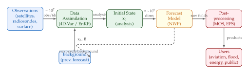
Operational NWP systems
The world's major operational NWP centres maintain global models that run multiple times per day, 365 days per year, and provide the backbone of public weather forecasts. Table 2 summarises the key operational systems as of 2024.
| System | Centre | Det. res. | Ens. members | Top level | Dynamical core |
| IFS (HRES) | ECMWF | 1 (det.) | Spectral + SL | ||
| IFS (ENS) | ECMWF | 50 | Spectral + SL | ||
| GFS | NOAA/NCEP | 1 (det.) | FV3 (cubed sphere) | ||
| GEFS | NOAA/NCEP | 30 | FV3 (cubed sphere) | ||
| UM (MOGREPS-G) | UKMO | 18 | ENDGame (semi-impl.) | ||
| ICON | DWD/MPI-M | 40 (ICON-EPS) | Icosahedral FV | ||
| GSM | JMA | 27 (GEPS) | Spectral + SL | ||
| SL = semi-Lagrangian; FV = finite volume; det. = deterministic; ens. = ensemble; res. = resolution. | |||||
| ECMWF's AIFS (AI model) runs alongside IFS but is not listed as it uses a different paradigm. | |||||
ECMWF IFS.
The European Centre for Medium-Range Weather Forecasts (ECMWF) Integrated Forecasting System is widely considered the world's most accurate global NWP model, consistently outperforming competing systems on objective verification metrics over the 10-day range. It uses a spectral dynamical core with TCo1279 () for deterministic and TCo639 () for ensemble forecasting, 4D-Var data assimilation, and runs on the ECMWF supercomputer in Bologna (currently ,petaflop/s sustained).
NOAA GFS.
The Global Forecast System is the primary operational model of the US National Centers for Environmental Prediction (NCEP), updated to the FV3 dynamical core on the cubed sphere in 2019. GFS data are freely available in near-real time, making it the primary training target for many ML weather benchmarks.
UKMO UM.
The UK Met Office Unified Model uses a non-hydrostatic, semi-implicit, semi-Lagrangian dynamical core (ENDGame) and the same model code from global scales down to storm-resolving nest domains-the “unified” philosophy. The probabilistic MOGREPS-G ensemble provides calibrated uncertainty estimates.
ICON.
The ICosahedral Nonhydrostatic model, developed jointly by the German Weather Service (DWD) and the Max Planck Institute for Meteorology, is the primary example of a production icosahedral-grid model. ICON is fully non-hydrostatic and can be run from global scales down to cloud-resolving resolution without changing the dynamical core.
JMA GSM.
The Japan Meteorological Agency's Global Spectral Model is the primary NWP model for East Asia and the western Pacific, where the JMA provides authoritative guidance on typhoon track and intensity.
Ensemble forecasting and uncertainty quantification
The atmosphere is a chaotic system: tiny differences in initial conditions amplify exponentially, so that after days even a perfect model loses all predictive skill. This predictability limit (the Lorenz limit) means that a single deterministic forecast is incomplete: it provides no information about forecast uncertainty.
Ensemble forecasting addresses this by running forecasts from slightly perturbed initial conditions (and, in modern systems, stochastic perturbations to the model physics): (Ensemble) where are carefully constructed initial perturbations (singular vectors, bred vectors, or EnKF perturbations) and – members. The ensemble mean approximates the expectation, and the ensemble spread provides a flow-dependent estimate of forecast uncertainty. Ensemble forecasting has transformed operational meteorology from deterministic prediction to probabilistic weather forecasting, enabling products such as probability of precipitation, percentile temperature forecasts, and severe weather risk maps.
Key Idea.
NWP is 70 years of hard-won physics and numerical mathematics AI-based weather models (Chapter 39, Sections 5–8) have achieved remarkable forecast skill by training on ERA5 reanalysis data and learning to approximate the mapping . But this success rests on a foundation of 70 years of hard-won physics and numerical mathematics:
The primitive equations encode conservation laws, rotation effects, and thermodynamics developed from first principles over more than a century.
ERA5, the primary training data for AI models, is itself the output of a sophisticated NWP data assimilation system-AI models are, in effect, learning from NWP, not from raw observations.
Verification protocols, evaluation datasets, and physical consistency checks (conservation of mass and energy, geostrophic balance, precipitation physics) were developed by the NWP community and are essential for assessing AI model quality.
The failure modes of AI weather models (spectral truncation artefacts, hallucinated precipitation, unphysical vertical profiles) can only be diagnosed and corrected with the physical understanding provided by NWP science.
NWP is 70 years of hard-won physics and numerical mathematics that AI must build on, not replace. The most promising future systems will be hybrid: AI components embedded within or trained with guidance from the physical equations, combining the generalisation power of deep learning with the physical fidelity of NWP.
Exercises for Section Numerical Weather Prediction Foundations
Exercise 10.
Consider a global spectral NWP model with T639 truncation () using a semi-implicit semi-Lagrangian scheme with time step .
The CFL condition for explicit Eulerian advection requires . For gravity wave speed , what is the maximum stable time step for an explicit scheme at this resolution?
By what factor does the semi-implicit semi-Lagrangian scheme allow the time step to exceed the explicit CFL limit?
The forecast model runs for 10 days. Compute the total number of time steps required. If each time step takes 2.5 seconds of wall-clock time on the supercomputer, how long does the 10-day forecast take to produce?
Exercise 11.
A global EnKF system uses ensemble members on a model with state variables and assimilates observations every 6 hours.
Compute the total memory required to store the full ensemble matrix in 32-bit floating point. Compare this to the memory required for the full background covariance matrix in 32-bit floating point.
The Kalman gain computation requires forming . Explain why this is infeasible to store directly, and describe the ensemble space approach that reduces the effective dimension of this system from to .
A proposed AI surrogate replaces the 80-member ensemble with a single forward pass of a diffusion model conditioned on the current analysis. Discuss two physical requirements that such a surrogate must satisfy to be a valid replacement.
Exercise 12.
ERA5 provides hourly atmospheric state estimates on a () global grid with 137 pressure levels and covers 1940–present.
Estimate the number of grid points in the ERA5 three-dimensional global grid. If each grid point stores prognostic variables in 32-bit floating point, what is the storage per hourly snapshot?
ERA5 is described as a “reanalysis”, not a pure observational record. Explain three ways in which ERA5 data differ from direct atmospheric observations, and discuss implications for training AI weather models.
In the pre-satellite era (before 1979), ERA5 has far fewer assimilated observations, particularly over the ocean and Southern Hemisphere. How would you expect the quality of ERA5 to differ between 1950 and 2010? What does this imply for AI weather models that train over the full 1940–present period?
Model Output Statistics and Early Post-Processing
By the early 1970s, numerical weather prediction had achieved a remarkable technical milestone: operational atmospheric models were running daily at major meteorological centres around the world, producing gridded forecasts of temperature, wind, humidity, and precipitation on scales of hundreds of kilometres. Yet operational forecasters faced a persistent and embarrassing problem. The model output was systematically wrong in ways that were entirely predictable. Temperature forecasts at Denver, Colorado were routinely too warm because the coarse model grid smoothed the sharp elevation gradients of the Rocky Mountain Front Range. Precipitation probabilities at coastal stations were biased because the model could not resolve mesoscale orographic lifting. Wind speeds at airport sites were consistently underestimated because the aerodynamic roughness of urban terrain was absent from the land-surface parameterisation.
The operational forecaster could see these errors accumulating. They knew, from years of experience, that the model always ran cold in the San Joaquin Valley in summer, always ran dry over the Appalachian windward slopes in winter, always underforecast the morning low at coastal stations. But there was no systematic framework for correcting these biases – only institutional memory, forecaster experience, and manual adjustment.
It was into this gap that Harry Glahn and Dale Lowry stepped in 1972 with a paper that would reshape operational meteorology for the next five decades.
The Glahn–Lowry Paper and the MOS Framework
The fundamental insight of Glahn and Lowry was to treat the relationship between NWP model output and observed weather at a specific surface station as a statistical estimation problem. Rather than attempting to correct the model's physics – an enormously difficult task – one could instead learn a statistical mapping from model-predicted quantities to locally observed quantities, using historical pairs of model forecasts and verifying observations.
This idea rested on three prior observations. First, model errors are not random; they are systematic, location-specific, and seasonally varying. Second, the model's large-scale fields contain genuine skill – correctly capturing synoptic-scale patterns such as frontal passages, cyclone tracks, and upper-level ridges – even when local surface variables are poorly forecast. Third, multiple model output fields (upper-level temperatures, geopotential heights, absolute vorticity, precipitable water) contain complementary information about local weather conditions that no single predictor captures alone.
These three observations collectively motivate the use of multiple linear regression applied to a carefully selected subset of model output fields as predictors of a surface meteorological variable of interest. The method Glahn and Lowry developed for selecting this subset – screening regression – became the methodological core of operational MOS.
Definition 10 (Model Output Statistics).
Let denote a vector of predictors derived from numerical weather prediction model output at a forecast lead time , and let denote a scalar predictand – an observed meteorological quantity at a specific surface station. Model Output Statistics (MOS) is the family of statistical post-processing methods that estimate as a function (Basic) where is fitted by regression over a developmental sample of historical model–observation pairs . In its classical linear form, (Linear) where predictors are chosen by a sequential screening procedure that maximises reduction in mean-squared error at each step.
The definition captures several important degrees of freedom that distinguish MOS from naive bias correction. First, the predictor vector may contain not only the model's direct forecast of the predictand (e.g., the model's 2-metre temperature forecast) but also indirect predictors: upper-level temperatures, thickness values, vorticity, relative humidity at multiple pressure levels, and even squared or product terms formed from primary predictors. Second, the mapping is station-specific: a separate regression equation is fitted for each station and each forecast lead time. Third, the mapping implicitly performs both bias correction (removing systematic mean errors) and downscaling (bridging the spatial resolution gap between the coarse model grid and the point observation).
Sequential Screening Regression
The central algorithmic challenge in MOS equation development is predictor selection. A modern NWP model may produce forecasts of hundreds of variables at dozens of pressure levels and multiple lead times, yielding a predictor pool of potentially thousands of candidates for a single predictand. Including all predictors in the regression would produce severe overfitting on the developmental sample and numerically unstable coefficient estimates.
The solution adopted by Glahn and Lowry – and still used in operational MOS development today – is sequential forward screening, a greedy procedure that builds the regression equation one predictor at a time.
Algorithm 1 (Sequential Forward Screening for MOS).
Initialise. Let be the current predictor set and be the baseline mean-squared error (variance of the predictand).
Screen. For each candidate predictor , compute the reduction in mean-squared error that would result from adding to the current regression equation.
Select. Add with to , provided exceeds a prescribed entry threshold (typically corresponding to a partial -test -value below ).
Check retention. Retest all predictors already in via partial -tests; remove any whose marginal contribution has fallen below a retention threshold.
Iterate. Return to step 2 until no candidate predictor meets the entry criterion, or until a prescribed maximum number of predictors is reached (typically in classical MOS).
The screening algorithm is conservative by design. The entry and retention criteria prevent the inclusion of predictors whose apparent skill is an artefact of the finite developmental sample rather than genuine meteorological signal. The check-retention step (step 4) is particularly important: as new predictors enter the equation, previously entered predictors may become redundant due to multicollinearity, and their removal improves the equation's out-of-sample performance.
The result of the screening procedure for a specific station, predictand, and lead time is a small set of regression coefficients that defines the MOS equation. These coefficients are stored and applied in real time: when the NWP model produces a new forecast, the predictor values are extracted, fed into the equation, and the local station forecast is produced within seconds.
Predictands: Temperature, Precipitation, and Wind
Operational MOS systems develop separate equation sets for each predictand. The three predictand families of greatest economic and social importance are surface temperature, precipitation occurrence and amount, and wind.
Temperature predictands.
The most important temperature predictands are maximum daytime temperature () and minimum overnight temperature () at the 2-metre standard observation height. These quantities drive energy demand, agricultural frost risk, human health impacts, and transportation planning. Classical MOS predictors for include the model's 850-hPa temperature (which is largely free of surface boundary-layer errors), the model's 2-metre temperature (which carries the direct low-level information despite its biases), 1000–500-hPa thickness (a proxy for the mean tropospheric temperature), relative humidity, and the sine and cosine of the day of year (to capture seasonal residual biases after the climatological mean is removed).
Precipitation predictands.
The primary precipitation predictand in classical MOS is the probability of precipitation (PoP), defined as the probability that measurable precipitation ( inches) occurs within a specified time window (typically 12 or 24 hours) at or near the forecast station. Because PoP is a probability rather than a continuous quantity, the linear regression output must be transformed; the classical approach uses a linear regression for a conditional expectation and then truncates predictions to , though in practice the regression coefficients are chosen so that the fitted values naturally fall within a physically plausible range. More sophisticated extensions include the use of logistic regression or probit regression applied to a dichotomous (occurrence/non-occurrence) observation.
Wind predictands.
Wind is the most challenging classical MOS predictand because it is inherently two-dimensional and exhibits strong non-Gaussianity due to the directional wrapping of the wind rose. Operational MOS systems typically forecast wind speed and wind direction separately, using the model's 10-metre wind components and as primary predictors but also including terrain-adjusted wind exposure indices, mixing-layer depth, and roughness-length corrections specific to each station's exposure category.
Bias Correction and Downscaling
The two most important functions performed by MOS regression equations – beyond pure statistical prediction – are systematic bias correction and spatial downscaling. These are conceptually distinct but are accomplished simultaneously by the same regression coefficients.
Systematic bias correction.
Let denote the climatological mean of the predictand at the station and denote the long-run mean of the primary model predictor. If the model has a systematic warm bias , the intercept term will adjust downward to compensate. More precisely, taking expectations of the MOS equation over the developmental sample: (Unbiasedness) so the MOS forecast is unbiased over the developmental period by construction. This is the climatological unbiasedness property of ordinary least-squares regression, and it guarantees that MOS forecasts will not exhibit the systematic warm or cold biases present in the raw NWP output.
Spatial downscaling.
The NWP model produces forecasts on a grid with spacing of order 10–100 km in operational systems. A surface station may sit at an elevation, land-surface type, or coastal proximity that differs substantially from the grid-cell average. The MOS regression coefficients encode this discrepancy implicitly: if the station sits in a valley that is systematically 3C cooler than the surrounding plateau that dominates the model grid cell, that constant offset is absorbed by the regression intercept ; a slope different from unity instead encodes an amplified or damped sensitivity of the station to the large-scale thermal signal. No explicit terrain correction is applied; the statistics of the developmental sample speak for themselves.
Remark 10.
The implicit downscaling accomplished by MOS is both its greatest strength and its greatest weakness. It is a strength because it requires no knowledge of the physical mechanism responsible for the local anomaly – the statistics encode whatever causal relationship exists. It is a weakness because it can only correct for stationary local effects: those that are present consistently enough in the developmental sample to appear as a stable statistical relationship. Climate change, station relocation, and changes in land use can all invalidate the developmental-sample statistics and introduce new biases that MOS cannot detect or correct without retraining.
Example: MOS Equations for Maximum Temperature
To make the abstract framework concrete, consider a hypothetical MOS equation for maximum temperature ( in F) at a mid-latitude inland station, valid 24–36 hours after model initialisation. After screening from a pool of 312 candidate predictors, suppose the screening algorithm selects the following five predictors:
| Variable | Description | Pressure level | |
| 2-metre temperature | Surface | ||
| Temperature | 850 hPa | ||
| 1000–500 hPa thickness | – | ||
| Relative humidity | 700 hPa | ||
| – |
The fitted MOS equation takes the form: (TMAX Example) where is expressed in decametres and in per cent.
Several features of equation are worth noting. The dominant predictor is , the model's own 2-metre temperature forecast, with a coefficient less than unity: this is regression attenuation, since the noisy predictor makes the least-squares fit shrink its slope toward the mean, so the regression pulls the model's temperature slightly toward the climatological mean. The 850-hPa temperature provides an independent estimate of the synoptic thermal environment, adding skill beyond alone because the 850-hPa level is largely above the boundary layer and hence less affected by surface parameterisation errors. The negative coefficient on (mid-tropospheric relative humidity) captures the physical relationship between cloud cover (which suppresses maximum temperatures) and moisture. The seasonal harmonic corrects for residual seasonal biases that persist after the large-scale predictors are included.
The MOS Pipeline: From NWP Output to Local Forecast
Figure 6 illustrates the complete operational MOS workflow, from NWP model output through predictor extraction, regression application, and local forecast dissemination.
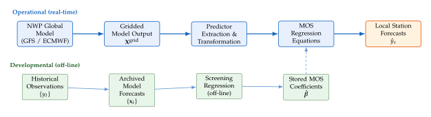
SAPEMOS and Regional Variants
The original Glahn–Lowry MOS framework was developed for the United States and relied on the dense observational network and long archive of NWP model runs that the National Weather Service had accumulated. Applying MOS in regions with sparse observational networks, short model archives, or less consistent station records required significant methodological adaptation.
SAPEMOS (South African Probabilistic Ensemble MOS) is a regional adaptation developed to provide probabilistic surface weather forecasts for southern Africa, where the observational network is far less dense than in North America or Europe. SAPEMOS addresses the data-sparsity problem through several innovations. First, it uses ensemble NWP output (rather than a single deterministic forecast) as the predictor set, so that forecast spread is available as an additional predictor alongside the ensemble mean; this allows the regression to encode the relationship between model uncertainty and forecast skill. Second, it employs spatial pooling across nearby stations to augment the effective developmental sample size, using station-specific dummy variables and elevation-adjusted corrections to retain station-specific information while borrowing statistical strength from the regional pool. Third, it outputs full probability distributions over the predictand rather than point forecasts, matching the needs of decision-makers in sectors such as agriculture, water management, and disaster preparedness.
Example 2 (SAPEMOS precipitation probability).
Let denote the predictor matrix formed from an ensemble of NWP members, each providing output variables. SAPEMOS forms ensemble-derived predictors by stacking the ensemble mean and ensemble standard deviation into an augmented predictor vector . The probability of exceeding a precipitation threshold is then modelled as (Logistic) where and are fitted by penalised logistic regression over the developmental sample of pooled station–season pairs. The ensemble spread predictors in allow the probability estimate to widen when the NWP ensemble is more uncertain, providing calibrated probabilistic output rather than a single probability estimate.
Classical Statistical Ensemble Post-Processing
The shift from single deterministic NWP runs to ensemble NWP systems – multiple model runs with perturbed initial conditions and model parameters – opened a new chapter in statistical post-processing. An ensemble is, in principle, a probabilistic forecast: the spread of ensemble members should encode forecast uncertainty. In practice, however, raw ensembles are both underdispersive (their spread is too narrow, underestimating uncertainty in smooth flows) and biased (systematic errors in initial perturbations and model parameterisations shift the ensemble mean away from the true state). Classical statistical ensemble post-processing methods were developed to correct these deficiencies.
Bayesian Model Averaging (BMA).
Raftery and colleagues introduced Bayesian Model Averaging (BMA) for weather forecasts in a landmark 2005 paper. The BMA approach treats each ensemble member as generating a conditional predictive distribution for the observation, and the overall predictive distribution is a weighted mixture: (BMA) where , are mixture weights fitted by maximum likelihood (via the EM algorithm) over a training window, and is a Gaussian predictive density centred at a bias-corrected version of ensemble member .
Ensemble Model Output Statistics (EMOS).
Gneiting and colleagues proposed EMOS (also called Non-homogeneous Gaussian Regression, NGR) as a more parsimonious alternative to BMA. Rather than fitting a mixture distribution, EMOS fits a single Gaussian whose mean and variance are affine functions of the ensemble mean and variance: (EMOS) where is the ensemble mean, is the ensemble variance, and are fitted parameters. The parameters are estimated by minimising the continuous ranked probability score (CRPS) over a rolling training window.
Non-homogeneous Gaussian Regression (NGR).
NGR is essentially a synonym for EMOS, emphasising the statistical interpretation: the predictive variance is allowed to be a function of the ensemble spread (hence “non-homogeneous”), unlike classical homoscedastic regression where the residual variance is constant. This flexibility is critical for ensemble post-processing because the model's predictability varies substantially by weather regime: zonal, predictable flows yield small ensemble spread and tight predictive distributions, while amplified blocked patterns yield large spread and broad distributions.
Remark 11.
The use of CRPS as the fitting criterion for EMOS is not coincidental. CRPS is a proper scoring rule: it is minimised in expectation when the predictive distribution equals the true conditional distribution of the observation. This means that fitting by CRPS encourages calibrated probability forecasts rather than merely accurate point forecasts – a crucial distinction in operational meteorology where downstream users make risk-weighted decisions.
Limitations of Linear MOS
For all its practical success, classical linear MOS carries fundamental limitations that became increasingly apparent as operational forecasters pushed into higher-resolution, higher-stakes prediction problems.
Linearity.
The central assumption of MOS is that the relationship between model output predictors and local observations is well approximated by a linear combination. This assumption is reasonable for large-scale temperature and thickness predictors, where the relationship is genuinely quasi-linear over synoptic scales. But it fails for a broad class of meteorologically important phenomena. Convective initiation – the transition from a stable, cloudless atmosphere to active convective precipitation – is intrinsically nonlinear: small changes in lower-tropospheric moisture and stability can flip the atmosphere from suppressed to convectively active within hours, a bifurcation that no linear model can represent.
Interactions.
A linear regression cannot capture the interaction between predictors. Severe wind gusts at a coastal station depend not on wind speed or atmospheric stability alone, but on their joint configuration: a marine layer that is both deep and strongly stable traps coastal jets more effectively than either condition alone. The product term could in principle be added as a new predictor, but the curse of dimensionality quickly limits the number of interaction terms that can be included without overfitting on the developmental sample.
Spatial structure.
Classical MOS equations are fitted independently for each station, ignoring the spatial correlation structure of the atmosphere. Two stations 50 km apart share large fractions of their forecast error, and a method that models them jointly could exploit this correlation to improve both forecasts. Station-independent regression discards this information.
Regime dependence.
The statistical relationship between model output and observations can change dramatically between weather regimes. A regression equation fitted on climatological averages of all regime types will perform poorly in any specific regime, particularly extreme events where the atmosphere is furthest from its climatological state and where forecast accuracy matters most.
Caution.
These limitations of linear MOS are not merely technical inconveniences; they reflect a fundamental ceiling on the skill achievable by linear statistical post-processing. The nonlinear interactions, spatial dependencies, and regime sensitivities of the atmosphere require methods capable of learning complex, high-dimensional functional relationships – precisely the territory of machine learning, to which the remainder of this chapter and the following sections are devoted.
Historical Note: Harry Glahn at NOAA-MDL
Historical Note.
Harry Glahn and the Birth of MOS, 1972–2012.
Harry R. Glahn spent his entire career at the National Oceanic and Atmospheric Administration's Meteorological Development Laboratory (NOAA-MDL) in Silver Spring, Maryland, retiring in 2012 after four decades of contributions to statistical weather forecasting. His 1972 paper with Dale Lowry, “The Use of Model Output Statistics (MOS) in Objective Weather Forecasting,” published in the Journal of Applied Meteorology, introduced both the term “Model Output Statistics” and the methodological framework that would underpin operational US weather forecasting for the next half century.
Glahn's insight was that the growing power of numerical weather prediction could be harnessed not only through physical model improvement but through systematic statistical learning from model errors. At a time when machine learning did not exist as a field and “big data” was decades away, Glahn built MOS on the modest but reliable tools of linear regression and classical statistics. The result was remarkably durable: variants of the original screening regression approach continued to be used operationally at NOAA-MDL well into the 2010s, and the MOS equations for the Global Forecast System (GFS) model produced forecasts that outperformed raw NWP output by statistically significant margins at virtually every US station.
Glahn's other contributions included the development of the Model Output Statistics Message (MOSM) format, which allowed MOS forecasts to be transmitted to weather offices in a compact binary format, and foundational work on the probabilistic interpretation of MOS output. He was awarded the American Meteorological Society's Award for Outstanding Contribution to the Advance of Applied Meteorology in 2000.
Exercises
Exercise 13.
Let denote the observed maximum temperature at a station on day and let denote the NWP-predicted 2-metre temperature and 850-hPa temperature respectively. Derive the ordinary least-squares estimator for the two-predictor MOS equation , and show that the fitted values are unbiased over the developmental sample (i.e., ). What happens to the unbiasedness property if the regression is fitted without an intercept term?
Exercise 14.
The Continuous Ranked Probability Score (CRPS) for a predictive distribution and scalar observation is defined as (CRPS) Show that for a Gaussian predictive distribution , the CRPS has the closed form where , is the standard normal density and is the standard normal CDF. Verify that with equality only when is the point mass at .
Exercise 15.
In the SAPEMOS logistic regression model , the augmented predictor vector includes both ensemble mean and ensemble standard deviation . Explain intuitively why including as a predictor can improve probabilistic calibration even when has low correlation with the observation itself. Under what meteorological conditions would you expect the ensemble spread to carry the most additional information beyond the ensemble mean?
Early Machine Learning in Meteorology
The closing years of the twentieth century brought a surge of interest in applying artificial neural networks to meteorological problems. The appeal was obvious: neural networks are universal approximators, capable in principle of learning arbitrary nonlinear mappings from input to output, and the limitations of linear MOS that we documented in the previous section were precisely the limitations that nonlinear function approximation promised to cure. Convective initiation, regime-dependent forecast skill, complex multiway predictor interactions – all of these phenomena involve nonlinearities that a sufficiently expressive neural network could in principle capture.
The reality, as we shall see, was more complicated. The neural networks of the 1990s and early 2000s were shallow – almost universally single-hidden-layer multilayer perceptrons trained by backpropagation. They were trained on modest datasets that were large by the standards of their era but tiny by those of modern deep learning. They ran on hardware orders of magnitude slower than contemporary GPUs. And they were applied to a forecasting problem whose spatiotemporal complexity would not be revealed until convolutional and recurrent architectures, trained on continental- scale radar archives, arrived two decades later.
Nevertheless, the early ML literature in meteorology is far from insignificant. It established the conceptual vocabulary of learned weather prediction, documented the first systematic experiments with nonlinear post-processing, and laid intellectual groundwork on which deep learning methods would later build. Understanding why these early methods were ultimately limited – and what was needed to overcome those limits – is essential context for appreciating the deep learning revolution in weather forecasting.
Key Idea.
Early machine learning in meteorology was fundamentally post-processing, not forecasting. The neural networks of the 1990s and 2000s took NWP model output as input and learned to correct or refine it, just as MOS did, but with nonlinear function approximators replacing linear regression. The idea of replacing the NWP model itself with a learned dynamical system – the aspiration of modern foundation models for weather – would not become computationally feasible for another two decades.
The First Wave: 1990s ANN Applications
The first serious applications of artificial neural networks to weather problems appeared in the early 1990s, driven by the renewed interest in connectionism that followed the rediscovery of backpropagation by Rumelhart, Hinton, and Williams in 1986. Meteorologists and environmental scientists were attracted by the promise of a nonlinear regression substitute that required no explicit specification of the functional form.
Chow and Leung (1996): Weather-Compensated Load Forecasting
An influential early application bridging meteorology and electrical engineering came from Chow and Leung, who in 1996 applied neural networks to short-term load forecasting – predicting electricity demand for grid management – with explicit weather-variable compensation.
The problem is meteorologically interesting because electricity demand depends nonlinearly on temperature: demand rises sharply for cooling at high temperatures and for heating at low temperatures, with a minimum in the mild temperature range. This U-shaped or V-shaped temperature–load relationship is precisely the kind of nonlinearity that linear regression handles poorly and that neural networks can in principle represent.
Chow and Leung used a two-stage network architecture. The first stage was a weather compensation module: a small MLP trained to predict the load residual attributable to temperature and humidity deviations from climatological norms, given the forecast temperature and humidity as inputs. The second stage was a base-load predictor that modelled the calendar-driven component of demand (day of week, hour of day, holiday flags). The outputs were combined linearly to produce the final load forecast.
The key contribution was demonstrating that the weather compensation could be learned automatically from historical data rather than parameterised analytically, and that the resulting nonlinear mapping outperformed linear regression-based weather adjustment on a dataset of Hong Kong hourly load observations. The authors reported mean absolute percentage errors that were reduced by 15–20% relative to the linear baseline in summer months, when the nonlinear cooling load dominated.
Hall, Brooks, and Doswell (1999): ANN Review for Meteorology
By the late 1990s, enough neural network studies had appeared in the meteorological literature to warrant a systematic review. Hall, Brooks, and Doswell published an influential survey in 1999 in the Weather and Forecasting journal that assessed the state of ANN applications across multiple meteorological problem domains: severe weather prediction, precipitation estimation, tropical cyclone intensity, and synoptic pattern recognition.
Several consistent findings emerged from the review. First, neural networks consistently outperformed linear regression on tasks with demonstrably nonlinear input–output relationships, with the largest improvements in heavy precipitation prediction and severe convective event discrimination. Second, the performance of neural networks was highly sensitive to the training sample size and composition: networks trained on climatologically balanced samples generalised poorly to rare extreme events because the extreme cases were underrepresented in the training data. Third, the “black box” nature of the single-hidden-layer MLP was a significant practical barrier to operational deployment: operational forecasters were reluctant to use tools whose internal reasoning they could not interrogate or verify.
The last finding anticipates a tension that remains unresolved in modern deep learning for weather: the trade-off between model expressiveness and interpretability. A linear MOS equation can be examined term by term; a forecaster can understand why the model predicted a warm day by looking at which predictors contributed most to the forecast. A neural network provides no such transparency.
Fuzzy and Bayesian Approaches
Chen and Hwang (2000): Fuzzy Time Series for Temperature
Alongside neural network approaches, the late 1990s and early 2000s saw a parallel tradition of fuzzy time series methods applied to meteorological forecasting. Chen and Hwang extended Song and Chissom's fuzzy time series framework to the problem of temperature prediction, introducing a method that represented historical observations as fuzzy sets and used fuzzy relational equations to model the temporal dynamics.
The approach partitioned the historical temperature range into a set of fuzzy linguistic variables (e.g., “very cold”, “cold”, “mild”, “warm”, “very hot”), defined membership functions for each linguistic variable, and then estimated a fuzzy transition matrix encoding the conditional probability that a temperature classified as “mild” today transitions to “warm” tomorrow. Forecasting consisted of applying the fuzzy matrix to the fuzzified current observation and defuzzifying the result to obtain a crisp temperature prediction.
The method's attraction was its interpretability: the fuzzy rules had a natural linguistic interpretation that could in principle be examined and validated by domain experts. Its limitation was its inability to use information from more than one or two previous time steps without an exponential explosion in the size of the fuzzy relational matrix.
Cofino et al. (2002): Bayesian Networks for Probabilistic Weather
A more principled probabilistic approach appeared in 2002 with the work of Cofino and colleagues, who applied Bayesian networks – directed acyclic graphs encoding conditional independence relationships between random variables – to the prediction of precipitation occurrence and amount at Spanish meteorological stations.
The Bayesian network framework represented the joint distribution of NWP predictors and surface observations as a factored product: (Bayesnet) where denotes the parent nodes of in the directed graph and the factorisation structure encodes the meteorologist's prior beliefs about which NWP fields causally influence which surface observations.
The key advantage over MOS was the ability to represent complex joint distributions over multiple simultaneous predictands and to propagate probabilistic uncertainty through the network. If the 500-hPa geopotential height was uncertain (as in an ensemble forecast), that uncertainty could be propagated through the network structure to yield a predictive distribution for precipitation that reflected both the model uncertainty and the statistical relationship between the large-scale predictor and the local observation.
Schizas, Baboo, and Backpropagation Networks
The application of backpropagation networks to the specific problem of minimum temperature forecasting represents one of the most thoroughly documented threads in early ML meteorology. Schizas, in a series of studies conducted at the University of Cyprus, and Baboo and colleagues in subsequent independent work, systematically compared MLP architectures of varying depth and width on the problem of predicting next-day minimum temperature from NWP predictors and surface observations.
The findings were consistent across different geographic settings and data periods. A single-hidden-layer MLP with between 10 and 20 hidden units, trained by batch backpropagation with momentum, outperformed linear MOS on temperature predictands when the training period included multiple weather regimes. The improvement was largest for minimum temperature – the predictand most sensitive to boundary-layer processes that the NWP model parameterised crudely – and smallest for maximum temperature, where the large-scale synoptic predictors (850-hPa temperature, 1000–500-hPa thickness) captured most of the variance.
The networks were typically trained with 5–10 years of daily data, yielding training sets of order – samples. Generalisation to independent test periods was assessed by root-mean-squared error and mean absolute error. While the improvements over MOS were statistically significant at many stations, they were modest in absolute terms – typically 0.1–0.3 C reductions in RMSE.
Hsieh (2009): Nonlinear Methods for Environmental Science
The most comprehensive attempt to synthesise the scattered early ML literature in atmospheric and oceanic science came with the publication of William Hsieh's 2009 textbook Machine Learning Methods in the Environmental Sciences. Published by Cambridge University Press, the book provided the first systematic treatment of neural networks, kernel methods, self-organising maps, and related techniques from the perspective of a practicing atmospheric scientist.
Hsieh's central contribution was to give the disparate ML applications in meteorology a unified statistical foundation. He showed that MOS could be seen as a special case of the broader framework of nonlinear regression, that Bayesian methods provided a principled approach to uncertainty quantification, and that the overfitting problems observed empirically in early neural network studies could be understood through the lens of the bias–variance trade-off.
Remark 12.
Hsieh's textbook appeared at a significant inflection point. Published in 2009, it represented the state of the art in ML for environmental science just before the deep learning revolution began to accelerate: AlexNet (2012), the availability of large GPU clusters, and the accumulation of continental-scale atmospheric data archives. The methods it covered – shallow networks, kernel SVMs, principal component analysis – would be largely superseded within five years by deep architectures that could exploit spatial and temporal structure in ways that single-hidden-layer MLPs could not.
The Limits of Shallow Networks
To understand why the early ML approaches in meteorology remained marginal – improving on MOS but never replacing it operationally – we must examine the specific limitations of shallow networks when applied to atmospheric data.
Vanishing gradients.
The standard activation function in 1990s neural networks was the logistic sigmoid or the hyperbolic tangent. Both functions saturate: for , the gradient . In networks with more than one or two hidden layers, the backpropagation gradient signal diminishes exponentially as it propagates from the output layer toward the input layer, making the early layers effectively untrainable. The practical consequence was that deep networks were inferior to shallow ones in the 1990s, not because depth was theoretically less powerful, but because the training algorithm failed to exploit it.
The vanishing gradient problem meant that early ML practitioners confined themselves to single-hidden-layer architectures. The universal approximation theorem guarantees that a single-hidden-layer network with sufficiently many units can approximate any continuous function, but the number of units required may be exponentially large in the input dimension. A single hidden layer of 20 units cannot capture the hierarchical spatial structure of a weather system – the synoptic scale pattern of ridges and troughs that organises the mesoscale convective structure that organises the microscale turbulent boundary layer – without an enormous number of parameters that the small training datasets of the era could not support.
No exploitation of spatial structure.
The single-hidden-layer MLP treats all inputs as exchangeable real numbers, with no structure imposed by the spatial proximity of adjacent grid points. A meteorological field – a 2-D array of temperature or geopotential values on a regular grid – contains rich spatial structure: nearby points are correlated, fronts appear as coherent oriented discontinuities, vorticity filaments have characteristic length scales. A fully connected MLP sees this field as a flat vector and must learn spatial relationships entirely from data, requiring far larger training sets than were available in the 1990s.
No capture of temporal dynamics.
Similarly, the early MLP architectures did not exploit the temporal structure of meteorological sequences. A weather state at time is not statistically independent of the states at times ; the atmosphere is a dynamical system, and its future state depends on its recent history. MLP architectures that use a fixed window of lagged inputs cannot generalise to longer-range dependencies and cannot represent the recurrent dynamics of developing weather systems.
Data scarcity.
Digital archives of NWP model output paired with surface observations were limited in the 1990s. Reanalysis products (ERA-Interim did not begin until 1979, and was not available until the late 2000s; NCEP/NCAR reanalysis extended to 1948 but at low resolution) provided modest training datasets by modern standards. The consequence was systematic undertraining of models with more than a few hundred free parameters.
Hardware constraints.
Training a neural network on 4,000 samples with 50 hidden units by backpropagation required hours on a workstation in 1996. Experimenting with multiple architectures, regularisation strengths, and predictor sets – the hyperparameter search that is routine today – was prohibitively expensive. Practitioners typically trained one or two architectures and reported results on the architecture that appeared to work best, a practice that inflated apparent gains and made inter-study comparisons unreliable.
Insight.
The fundamental ceiling on early ML in meteorology was not algorithmic – it was the conjunction of shallow architectures, small datasets, and slow hardware. Each of these limitations was necessary and jointly sufficient to suppress deep learning from emerging sooner. When GPUs reduced training time by three orders of magnitude, internet-scale data archives became accessible, and deep architectures with rectified linear units solved the vanishing gradient problem, the ceiling dissolved – not gradually, but essentially overnight.
The ConvLSTM Breakthrough: Shi et al. (2015)
The transition from shallow post-processing networks to deep spatiotemporal architectures for weather forecasting has a remarkably precise historical date: 2015, the year of the ConvLSTM paper by Shi and colleagues at the Hong Kong University of Science and Technology.
The problem they addressed was radar nowcasting: predicting the spatial structure of radar-observed precipitation at lead times of 0–2 hours. This is a qualitatively different problem from the MOS and ANN applications surveyed above. It is not a post-processing problem (there is no NWP model whose output is being corrected); it is a direct spatiotemporal prediction problem, mapping a sequence of past radar images to a sequence of future radar images.
Definition 11 (ConvLSTM Cell).
A Convolutional LSTM (ConvLSTM) cell generalises the standard LSTM cell by replacing the matrix–vector products with convolution operations. For input tensor , hidden state , and cell state (all spatial tensors of shape ), the ConvLSTM transitions are: (Gates) where denotes spatial convolution, denotes elementwise multiplication, and is the logistic sigmoid. The convolutional weight tensors (and analogues for other gates) are shared across all spatial positions, enforcing translational equivariance.
The key insight is that spatial convolution replaces matrix multiplication at every gate, so the hidden state and cell state remain spatial tensors rather than collapsing to vectors. This preserves the spatial structure of the input throughout the temporal unrolling, avoiding the information destruction that occurs when a fully connected LSTM flattens a spatial field to a vector.
Shi et al. trained a stacked ConvLSTM on the HKO-7 dataset, a 7-year archive of Hong Kong Observatory radar images at 6-minute intervals. The architecture used three ConvLSTM layers, each with filters of size , followed by a convolutional output layer predicting the next 20 radar frames (2 hours at 6-minute intervals).
The results were decisive. The ConvLSTM architecture outperformed ROVER (the optical-flow nowcasting baseline), LSTM (without convolution), and other deep learning baselines on all three evaluation metrics: CSI (Critical Success Index), FAR (False Alarm Rate), and POD (Probability of Detection). The improvement over the LSTM without convolution was particularly informative: it demonstrated that spatial structure was the critical missing ingredient, not just temporal depth.
Shi et al. (2017): TrajGRU and the HKO-7 Benchmark
In a 2017 follow-up, Shi and colleagues identified a limitation of the ConvLSTM: its convolutional connections are location-invariant (the same kernel is applied everywhere), which means the network implicitly assumes the same flow structure at every spatial location. Weather patterns, however, are inherently location-variant: a cyclone generates counterclockwise flow in the northern hemisphere, so the contribution of the state to the north differs systematically from the contribution of the state to the south.
The Trajectory GRU (TrajGRU) architecture they introduced replaced the fixed recurrent convolution with a learnable flow field: at each time step, the network predicted an optical-flow-like warp field that specified how to sample the previous hidden state when computing the current state. This sampling was implemented via bilinear interpolation, making the operation differentiable and compatible with standard backpropagation.
(WARP) where is predicted from and by a small convolutional sub-network, and denotes bilinear sampling at the positions displaced by . The TrajGRU cell then computes standard GRU transitions using in place of .
The same paper introduced a comprehensive benchmark evaluation framework for the HKO-7 dataset, defining standard train/validation/ test splits, evaluation metrics, and baselines (optical flow, ROVER, ConvLSTM). This benchmark infrastructure was an important contribution independent of the TrajGRU architecture itself: it provided a reproducible comparison point that subsequent methods could use, an example that the weather forecasting deep learning community would follow in establishing later benchmarks such as WeatherBench and ERA5-based evaluation suites.
MetNet and MetNet-2: Toward Continental-Scale Nowcasting
The conceptual arc from MOS through ConvLSTM reached a significant milestone with Google's MetNet (2020) and MetNet-2 (2021), presented in the paper by Sonderby and colleagues. These models extended the spatiotemporal deep learning paradigm to the full problem of precipitation probability forecasting over the continental United States at 1–8 km resolution, with lead times up to 8 hours (MetNet) and 12 hours (MetNet-2).
MetNet departed from the ConvLSTM paradigm in several important respects. First, it used a multi-scale convolutional encoder (based on a deep ResNet-style architecture with axial self-attention) rather than a recurrent architecture, extracting spatial context at multiple resolutions from a large spatial patch of radar and satellite observations. Second, it conditioned on the forecast lead time explicitly, using a learnable lead-time embedding that allowed a single model to produce forecasts at all lead times from 1 minute to 8 hours. Third, it was trained on a very large archive of MRMS (Multi-Radar Multi-Sensor) observations over the continental US, with years of training data covering diverse weather regimes.
Example 3 (MetNet-2 output representation).
MetNet-2 outputs a probabilistic precipitation rate at each grid point, represented as a categorical distribution over discretised precipitation bins. For bin boundaries (in mm/hr), the model outputs a softmax probability vector (the -simplex), where . A point estimate of the precipitation rate is recovered as where is the bin midpoint. This representation allows the model to capture the highly skewed, zero-inflated distribution of precipitation rates – with high probability mass at zero, a long right tail for heavy rain – without assuming any parametric form.
The MetNet-2 paper reported that at lead times up to 6 hours, the model outperformed HRRR (the High-Resolution Rapid Refresh NWP model) in terms of CSI and other standard metrics. This was a landmark result: a learned model, trained entirely from observations without any explicit atmospheric physics, had matched or exceeded a state-of-the-art operational NWP model at mesoscale precipitation nowcasting.
Remark 13.
Both MetNet and MetNet-2 remain constrained to lead times below 12 hours. Beyond this horizon, the lack of explicit atmospheric dynamics – the conservation laws, mass continuity, and pressure- wind balance that give NWP its physical consistency – limits the model's skill. For multi-day forecasts, purely data-driven models did not outperform NWP on standard metrics until 2022–2023, when foundation-model architectures such as Pangu-Weather and GraphCast surpassed operational NWP on many variables at those ranges (see Sections FourCastNet and the Spectral Revolution and following).
The Evolution of Architectures: From MOS to Transformers
Figure 7 charts the conceptual evolution from classical MOS through shallow ANNs, ConvLSTM, and transformer-based foundation models.
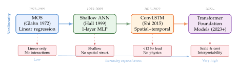
Comparison of Early ML Methods
Table 4 summarises the key characteristics and limitations of the early ML approaches surveyed in this section.
| Method | Spatial | Temporal | Probabilistic | Primary limitation |
| Linear MOS | No | No | Partial | Linearity; no interactions |
| Logistic/NGR | No | No | Yes | Parametric family assumption |
| BMA | No | No | Yes | Gaussian members; computational cost |
| Fuzzy time series | No | Partial | No | Exponential state space |
| Bayesian network | No | No | Yes | Manual graph elicitation |
| Shallow ANN (MLP) | No | No | No | Vanishing gradient; no spatial |
| ConvLSTM | Yes | Yes | No | Short lead time; no physics |
| TrajGRU | Yes | Yes | No | Short lead time; no physics |
| MetNet/MetNet-2 | Yes | Yes | Yes | 12-hour horizon |
The Transition from Shallow to Deep
The history surveyed in this section invites a natural question: why did the transition from shallow post-processing networks to deep spatiotemporal architectures take twenty years, and what eventually made it possible?
Insight.
The transition from shallow to deep learning in meteorology was not gradual – it required three simultaneous breakthroughs that arrived in rapid succession between 2012 and 2016. GPU hardware reduced neural network training time by three orders of magnitude. Large digital archives of reanalysis data (ERA-Interim, CFSR) and operational radar observations provided training datasets of sufficient size to train deep architectures without overfitting. And architectural innovations – rectified linear units eliminating the vanishing gradient problem, batch normalisation stabilising deep training, and convolutional architectures enforcing spatial equivariance – provided the modelling tools needed to exploit both the data and the hardware. Any one of these breakthroughs alone would have been insufficient; it was their conjunction that made deep learning for weather possible.
The forty-three years between Glahn and Lowry's 1972 paper and the 2015 ConvLSTM paper were not wasted. The early ML community established the problem formulation: that weather forecasting could be cast as a statistical learning problem with NWP output and observations as inputs and outputs. They documented the failure modes of linear and shallow nonlinear models, motivating the specific architectural innovations that would arrive later. And they built the evaluation infrastructure – standard datasets, metrics, and comparison baselines – on which the deep learning era would build.
What they could not provide was the essential technical substrate: the hardware, the data, and the architecture. These arrived in a compressed window between 2012 and 2017, and the field of weather forecasting has not been the same since.
Exercises
Exercise 16.
Consider a deep fully-connected neural network with hidden layers, each using the logistic sigmoid activation . Let denote the backpropagation error signal at layer . Show that , where are the layer- weights. Hence conclude that the gradient magnitude decreases geometrically with depth when all activations are in their saturating regime. How does switching to the ReLU activation modify this bound?
Exercise 17.
Derive the number of trainable parameters in a ConvLSTM layer with input channel dimension , hidden dimension , and convolutional kernel size . Compare this to the parameter count of a standard fully-connected LSTM taking as input the flattened spatial field of size and producing a hidden state of the same total dimension . For , , , and , compute the ratio of parameter counts. What is the practical implication of this ratio for training with limited data?
Exercise 18.
MetNet-2 outputs a categorical distribution over discretised precipitation bins. A simpler approach would be to output a single scalar (the expected precipitation) trained with mean-squared-error loss. Give two specific arguments, drawn from the properties of atmospheric precipitation fields, for why the categorical output representation is preferable to the scalar regression approach for operational forecasting applications. Your arguments should relate to the structure of the precipitation distribution, not merely to the general desirability of uncertainty quantification.
FourCastNet and the Spectral Revolution
The history of numerical weather prediction is in part a history of choosing the right basis. Richardson's finite-difference scheme (1922) tiled the atmosphere onto a rectilinear grid and advanced each cell forward in time by finite differences. It was correct in principle but required ten thousand human computers to advance a six-hour forecast for the northern hemisphere. Charney's spectral model (1949) transformed the governing equations into Fourier space, expressing every field as a superposition of spherical harmonics. The spectral formulation did not change the physics; it changed the algebra, converting the differential operators of the primitive equations into diagonal multiplications in frequency space. The ECMWF's Integrated Forecasting System (IFS) still relies on a spectral core for its dynamical equations.
The first generation of deep learning weather models-U-Net architectures trained to minimise mean-squared error-largely ignored this spectral heritage. They processed data on the physical grid, applying local convolution kernels that could only communicate information one receptive-field width at a time. The atmosphere is global: a blocking anticyclone over the Urals changes the phase of the North Atlantic Oscillation, which modulates precipitation over Britain, which alters the sensible-heat flux that feeds back into large-scale dynamics. Capturing these teleconnections requires global receptive fields, and achieving them with local convolutions requires either very deep networks or explicitly non-local attention.
Transformers offer global attention: every token communicates with every other token at each layer. But the cost of dense self-attention scales as in the number of tokens . At the resolution used by ERA5-, corresponding to a longitude-latitude grid-a weather state comprises spatial locations. Standard self-attention on this grid is computationally impossible. FourCastNet, introduced by Pathak et al. from NVIDIA in 2022, solved this problem by moving the token-mixing operation from physical space into Fourier (spectral) space, where global communication can be achieved in operations via the Fast Fourier Transform.
Complexity and the Case for Spectral Mixing
To understand why spectral processing is attractive for global atmospheric fields, consider the three main approaches to spatial mixing and their asymptotic costs on a two-dimensional grid of points, with channels.
Local convolution.
A convolution over a single channel pair requires multiply-add operations. The receptive field after layers grows as ; to achieve a global receptive field on a grid requires hundreds of layers. Communication is local; teleconnections emerge only indirectly.
Dense self-attention.
Treating each grid cell as a token, the attention matrix (where ) has entries. Computing the matrix product costs operations and memory. For this is prohibitive.
Spectral mixing (AFNO).
The Discrete Fourier Transform (DFT) of a signal of length can be computed in operations via the FFT. In Fourier space, convolution becomes pointwise multiplication; hence a global convolution-one whose kernel spans the full domain-costs only . The Adaptive Fourier Neural Operator augments this with a learned, frequency-wise mixing step, achieving global communication at cost, five orders of magnitude cheaper than dense attention for ERA5 resolution.
Key Idea.
Moving computation from physical space to spectral space collapses the cost of global attention. A dense self-attention over tokens costs . The FFT transforms those tokens into complex frequency coefficients in ; global mixing in Fourier space then costs ; and the inverse FFT maps back to physical space in . The total replaces the of dense attention, while retaining the property that every spatial location communicates with every other location at each layer.
Fourier Neural Operators: Mathematical Foundations
The Fourier Neural Operator (FNO), introduced by Li et al. (2021), provides the mathematical basis for spectral-domain learning. Let be a bounded domain (in weather applications, is the sphere discretised as a regular longitude-latitude grid). An FNO layer maps a function to a function via
(FNO Layer)
where is a pointwise linear map (the residual branch), is a nonlinearity applied elementwise, and is the integral kernel operator
(Integral Kernel)
By the convolution theorem, equation becomes, in Fourier space,
(CONV Theorem)
where denotes the Fourier transform and is a frequency index. The FNO parametrises as a learnable complex-valued tensor for each retained frequency . Only the lowest modes are learned; high-frequency components are zeroed (a soft truncation that acts as a spectral filter). The full FNO layer in discrete form is thus
(FNO Discrete)
where denotes the (fast) Discrete Fourier Transform and its inverse.
Definition 12 (Fourier Neural Operator Layer).
Let be an input feature map on a grid of spatial locations with channels. A Fourier Neural Operator (FNO) layer computes
(FNO DEF)
where is a pointwise weight matrix, is the spectral weight tensor retaining only the lowest frequency modes, denotes mode-wise matrix multiplication, and is a pointwise nonlinearity (typically GELU).
The key properties of the FNO layer that make it attractive for weather modelling are:
Global receptive field: every grid point communicates with every other via the Fourier transform.
Permutation equivariance: the layer is equivariant to translations of the input field.
Resolution invariance: the spectral representation is basis-independent; a model trained at one resolution can be evaluated at another by adjusting the number of retained modes.
Computational efficiency: the FFT costs , and the learned mixing costs , much less than for dense attention.
Adaptive Fourier Neural Operators
FourCastNet does not use FNO directly; it uses the Adaptive Fourier Neural Operator (AFNO), introduced by Guibas et al. (2021) as part of the FNet/AFNO line of work. The AFNO modifies the FNO in two key ways:
Token mixing via FFT: Rather than treating each channel independently, the AFNO applies the 2D FFT across spatial dimensions, treating the -dimensional feature vector at each frequency as a “token” and applying a shared MLP in frequency space.
Sparsity via soft-thresholding: The AFNO applies a learnable soft-thresholding operator to the Fourier coefficients, adaptively pruning frequency components that carry little information for the current input. This is the “adaptive” part.
Formally, let be the input feature map. The AFNO layer proceeds as follows:
Forward FFT: Compute .
Frequency-wise MLP: For each frequency bin , apply a two-layer MLP with hidden dimension (typically for efficiency): (AFNO MLP) where the MLP operates on the complex-valued channel vector at that frequency. The weights are shared across all frequency bins, giving translation equivariance.
Soft-thresholding (sparsification): Apply a learnable element-wise shrinkage: (SOFT Threshold) where is a learnable threshold per channel. This promotes sparsity in frequency space, concentrating representational energy in the most informative modes.
Inverse FFT: Compute .
Residual connection: Output .
Definition 13 (Adaptive Fourier Neural Operator).
An Adaptive Fourier Neural Operator (AFNO) layer with input , shared channel-mixing MLP , and per-channel thresholds computes
(AFNO FULL)
The total computational cost is for the FFT steps and for the frequency-wise MLP, where is the hidden dimension of the MLP.
Remark 14 (AFNO versus multi-head self-attention).
Standard multi-head self-attention (MHSA) on a sequence of tokens with embedding dimension costs for the attention computation. At ERA5 resolution, , so MHSA would cost roughly times as many token-mixing operations per layer as the AFNO (about five orders of magnitude, consistent with the estimate above). The AFNO achieves the same global receptive field-every spatial location is mixed with every other via the Fourier basis-at a fraction of the cost. The price paid is the loss of content-dependent weighting: the mixing weights in the AFNO MLP do not depend on the input values, only on the frequency index. FourCastNet empirically shows that this sacrifice is acceptable for short-to-medium range weather forecasting.
FourCastNet Architecture
FourCastNet (Pathak et al., 2022) is a vision-transformer-like architecture that replaces every attention layer with an AFNO layer. The full architecture proceeds in four stages.
Stage 1: Patch embedding.
Each atmospheric state is represented as a multi-channel field where , , and is the number of input variables (20 in FourCastNet-v1, including surface variables and pressure-level fields). The field is first partitioned into non-overlapping patches (patch size in the original model), and each patch is linearly projected to an embedding dimension :
(Patch Embed)
where is the embedding of patch , and are the projection weights and biases, and is a learnable positional embedding. After embedding, the field becomes a 2D array of tokens .
Stage 2: AFNO blocks.
The embedded tokens are processed by sequential AFNO blocks, each consisting of:
Layer normalisation (pre-norm);
An AFNO layer performing spectral token mixing;
A residual connection;
Layer normalisation;
A two-layer feed-forward MLP with expansion ratio and GELU nonlinearity;
A residual connection.
Letting denote the hidden state after block , the recurrence is
(AFNO Block)
for . FourCastNet-v1 uses AFNO blocks with embedding dimension .
Stage 3: Decoding to grid.
The final hidden state is projected back to the physical grid using a learned patch-expansion layer:
(Patch Expand)
where is the number of predicted output variables. The patch-expansion uses a transposed linear projection followed by a pixel-shuffle (sub-pixel convolution) to upsample from patch resolution to full grid resolution.
Stage 4: Autoregressive rollout.
FourCastNet is trained to predict the atmospheric state from for a fixed time step . For longer forecast horizons, the model is rolled out autoregressively: for
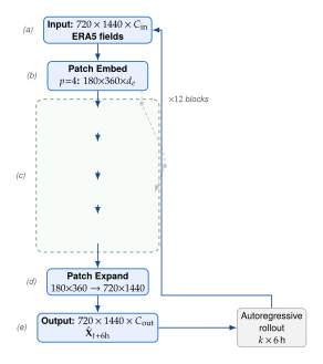
Training Data and Objective
Dataset.
FourCastNet is trained on the ERA5 reanalysis dataset produced by ECMWF. ERA5 provides hourly estimates of the global atmospheric state at horizontal resolution (approximately 28,km at the equator), with 37 pressure levels from 1000,hPa to 1,hPa. The training period spans 1979–2015, the validation set covers 2016–2017, and the test set covers 2018 onward.
The model uses 20 atmospheric channels, a sparse subset of variables and levels (not a full variable-by-level product):
Surface fields (5): 10-metre wind components , , 2-metre temperature , surface pressure, and mean sea-level pressure.
1000,hPa (3): , , geopotential .
850,hPa (5): , , , , relative humidity.
500,hPa (5): , , , , relative humidity.
50,hPa (1): ; and total column water vapour (1).
(The full level set listed for other models is Pangu-Weather's, not FourCastNet-v1's.)
Each channel is normalised per-level to zero mean and unit variance using statistics computed from the training split, ensuring equal gradient contributions from fields with very different physical magnitudes.
Loss function.
The training objective is the weighted mean-squared error
(Fourcastnet LOSS)
where is a channel-specific weight that up-weights physically important variables (e.g., geopotential is given higher weight than humidity), and is the area weighting for latitude , compensating for the convergence of meridians toward the poles where grid cells have smaller physical area.
The area weighting is crucial: without it, gradient contributions from high-latitude cells (which are small in physical area but numerous in the regular grid) would dominate training, causing the model to over-optimise polar regions at the expense of the tropics.
Multi-step fine-tuning.
FourCastNet is first trained with the single-step loss . It is then fine-tuned with a multi-step loss that includes up to 8 autoregressive steps, backpropagating through the rollout:
(Multistep LOSS)
where steps and is a discount factor that down-weights distant predictions. This fine-tuning phase is essential: without it, errors compound quickly during autoregressive rollout because the model was only trained to map ERA5 states to ERA5 states, not its own imperfect predictions to ERA5 states.
Worked Example: Seven-Day Surface Wind Forecast
Example 4 (Seven-day wind forecast with FourCastNet).
Suppose we wish to produce a 7-day (168-hour) forecast of 10-metre wind speed starting from 00:00 UTC on 1 September 2018.
Initialisation.
Download ERA5 analysis for 00:00 UTC 1 September 2018. This gives 20 channels on a grid. Normalise each channel using the training-set statistics : .
Rollout.
Apply FourCastNet autoregressively for steps:
Each forward pass through the -block FourCastNet takes approximately 0.15 seconds on a single NVIDIA A100 GPU. The full 7-day rollout (28 passes) therefore completes in about 4 seconds. A comparable IFS ensemble member at T1279 () spectral resolution requires roughly CPU-hours.
Reconstruction.
Denormalise the predicted and channels: . The 10-metre wind speed is .
Accuracy.
On the ERA5 test set (2018), FourCastNet achieves a latitude-weighted RMSE for at 5-day lead time of approximately , comparable to IFS () at 5 days. The speed-up factor exceeds (100,000) versus IFS at comparable resolution.
Performance Against Operational Forecasting
Pathak et al. (2022) evaluated FourCastNet against the ECMWF IFS high-resolution deterministic forecast (HRES) using latitude-weighted RMSE and anomaly correlation coefficient (ACC) on the 2018 test year. Key findings:
Geopotential : FourCastNet matches IFS HRES at lead times up to 5 days; IFS is superior at 7 days (FourCastNet shows 10% higher RMSE).
Surface wind , : FourCastNet matches IFS at 1–3 days; slight degradation at 5+ days.
Precipitation: FourCastNet performs substantially worse than IFS for total precipitation, because precipitation is poorly constrained in ERA5 (it is derived, not directly observed) and involves nonlinear convective processes that the deterministic regression objective cannot capture.
Speed: FourCastNet inference on a single A100 GPU produces a 7-day global forecast in under 5 seconds; IFS HRES requires approximately 150,000 CPU-hours on ECMWF's Atos supercomputer. The speed-up is five to six orders of magnitude.
Remark 15 (ERA5 smoothing and verification circularity).
Both FourCastNet and its evaluation target are based on ERA5. ERA5 is itself produced by a variational data-assimilation system that blends model forecasts with observations; it is therefore smoother than reality at small scales. Evaluating FourCastNet against ERA5 means measuring how well the model reproduces a smoothed, gridded analysis, not how well it predicts actual atmospheric states. This is an important caveat: FourCastNet is better characterised as an “ERA5 emulator” than a direct observation predictor.
FourCastNet-v2 and Scalable Geometric ML
The original FourCastNet established the AFNO paradigm. Two subsequent iterations significantly extended its capability.
FourCastNet-v2 (Bonev et al., 2023).
FourCastNet-v2 replaces the AFNO token mixer with a spherical Fourier neural operator (SFNO) that operates natively on the sphere using spherical harmonics as the Fourier basis. The motivation is geometric: the regular latitude-longitude grid treats the sphere as a flat rectangle, introducing distortions near the poles. Spherical harmonics (where is the degree, the order, the latitude, and the longitude) are the natural basis for functions on the sphere, satisfying .
The SFNO layer replaces the 2D FFT with the Spherical Harmonic Transform (SHT) and its inverse, and replaces the frequency-wise MLP with a degree-wise (rotationally equivariant) mixing:
(SFNO MIX)
where is a learnable coupling matrix between spherical harmonic degrees and . This formulation is equivariant to rotations of the sphere, a property the original Cartesian AFNO lacks. FourCastNet-v2 achieves improved accuracy at polar latitudes and better long-range teleconnection representation.
FourCastNet 3: Geometric Foundation Models.
Subsequent work (2024–2025) extended FourCastNet into a geometric foundation model framework, in which a single large model pre-trained on diverse atmospheric data (ERA5, MERRA-2, JRA-55, satellite radiances) can be fine-tuned for downstream tasks including:
Medium-range deterministic forecasting (days 1–10);
Subseasonal-to-seasonal prediction (weeks 2–8);
Downscaling to high-resolution regional grids via learned geometric interpolation operators;
Data assimilation, generating analysis states from sparse observations.
The architecture scales from 70M parameters (FourCastNet-v1) to 2B parameters (FourCastNet 3), with performance improvements following approximate power laws in parameter count, mirroring scaling behaviour observed in large language models.
Insight.
The AFNO-based approach demonstrates that the spectral heritage of classical NWP-rooted in Charney's 1949 spectral model-can be reincorporated into deep learning architectures, not as a rigid physical constraint but as a flexible inductive bias that dramatically reduces computational cost while preserving global spatial communication.
Exercises
Exercise 19 (FFT complexity on the ERA5 grid).
The ERA5 grid has latitude points and longitude points, giving spatial locations.
Show that the 2D FFT of a real-valued field on this grid can be computed in operations. Derive the exact operation count using the Cooley-Tukey algorithm, assuming and are highly composite numbers (which they are: , ).
Dense self-attention on the same grid treats each of the spatial locations as a token. Compute the ratio of the self-attention FLOPs to the AFNO FLOPs for and retained Fourier modes.
The AFNO frequency-wise MLP is shared across all frequency bins. How many learnable parameters does this MLP have if it has one hidden layer of width ? How does this compare to the parameter count of a single self-attention head?
Exercise 20 (Area weighting in the loss function).
The FourCastNet loss uses latitude-dependent area weights .
Derive from the requirement that the weighted mean of a spatially uniform field equals 1, i.e., for all when the field is constant. Why is the naive (unweighted) arithmetic mean biased toward polar regions?
For the ERA5 grid, compute the ratio (polar weight over equatorial weight). What does this ratio imply for gradient magnitudes in polar versus equatorial regions during training without area weighting?
Propose an alternative area-weighting scheme based on the Voronoi area of each grid cell on the sphere (the actual area in square kilometres), and compare it to the approximation. Under what conditions are the two schemes equivalent?
Exercise 21 (Autoregressive error growth).
Let denote the RMSE of the FourCastNet forecast at lead time (where ), and suppose that at each step the model introduces an independent error increment with variance .
Assuming errors add in quadrature (i.e., are independent across steps), show that . Empirically, FourCastNet RMSE for grows approximately as . What does the sub-linear exponent () suggest about the error-growth mechanism?
The multi-step fine-tuning loss uses a discount factor . Derive the optimal that minimises the expected RMSE at the maximum forecast horizon , under the independent-errors model from (a).
The spherical harmonic expansion of the forecast error field at step has power spectrum where is the spherical harmonic degree. Explain qualitatively why grows faster for large (small scales) than small (large scales), and discuss the implications for the spectral bias of AFNO-based models.
Pangu-Weather and 3D Transformer Architectures
In 2023, a paper published in Nature reported that a neural network had, for the first time, beaten the world's best operational numerical weather prediction system-ECMWF's Integrated Forecasting System-on over 90% of variables at all tested lead times. The model was called Pangu-Weather, developed by researchers at Huawei Cloud Research and Huawei Noah's Ark Laboratory, led by Kaifeng Bi and colleagues. The result was not a marginal improvement; at 5-day lead times, Pangu-Weather reduced the RMSE for 500-hPa geopotential by approximately 3% over IFS HRES while running ten thousand times faster.
The architectural leap that enabled this result was three-dimensionality. Where FourCastNet processed the atmosphere as a 2D field of horizontal patches-treating vertical levels as separate channels-Pangu-Weather introduced a genuine three-dimensional transformer that attends simultaneously over latitude, longitude, and pressure level. This apparently minor change has profound consequences: it allows the model to learn the vertical coupling that governs phenomena as diverse as tropical cyclone development, jet-stream variability, and the propagation of planetary waves from the stratosphere into the troposphere.
From Vision Transformers to Weather Transformers
Pangu-Weather's architecture has a clear lineage in computer vision.
Vision Transformer (ViT).
Dosovitskiy et al. (2021) introduced the ViT by treating an image as a sequence of non-overlapping patches and applying standard transformer self-attention. The key insight was that the inductive biases of convolutional networks (translation equivariance, local connectivity) could be abandoned in favour of global attention, with the model free to learn its own spatial inductive biases from data. ViTs achieve state-of-the-art performance on ImageNet with sufficient data, outperforming CNNs of comparable parameter count.
Swin Transformer.
Liu et al. (2021) observed that global attention in ViT scales as . The Swin Transformer replaces global attention with shifted window (SW) attention: each token attends only to tokens within a local window, reducing cost to for fixed window size . A “shift” mechanism introduces cross-window communication by shifting the window partition between consecutive layers. Swin won the ImageNet-22K top-1 accuracy benchmark in 2021 and became the dominant backbone for dense prediction tasks (detection, segmentation).
3D Swin Transformer.
The natural extension to video and volumetric data replaces 2D windows with 3D windows spanning height width time (or depth). Liu et al. (2022) introduced Video Swin for video recognition. Pangu-Weather adapts this idea to atmospheric data, where the three dimensions are latitude longitude pressure level.
The 3D Earth-Specific Transformer (3DEST)
The core of Pangu-Weather is the 3D Earth-Specific Transformer (3DEST), which differs from a standard 3D Swin Transformer in two critical respects: (1) it uses an Earth-specific positional bias that accounts for the non-uniform physical spacing of pressure levels and the spherical geometry of the planet; and (2) it processes upper-air and surface variables in separate streams that interact only at the decoding stage.
Input representation.
The full atmospheric state at a given time is represented as two tensors:
Upper-air tensor: , where 13 is the number of pressure levels (1000, 925, 850, 700, 600, 500, 400, 300, 250, 200, 150, 100, 50,hPa), , , and channels (geopotential , temperature , zonal wind , meridional wind , specific humidity ).
Surface tensor: , where channels (mean sea-level pressure , 10m wind , , and 2m temperature ).
Patch embedding.
The upper-air tensor is partitioned into patches (2 pressure levels 4 latitude points 4 longitude points), giving tokens. Each token is a -dimensional vector, linearly projected to embedding dimension . The surface tensor uses patches.
3D window attention.
The 3DEST divides the token grid into non-overlapping 3D windows of size (with typical values , , ). Standard self-attention is applied within each window:
(3D ATTN)
where are query, key, and value matrices for the tokens in the window, and is the Earth-specific relative position bias defined below.
The cost of 3D window attention is rather than ; for fixed window size this is linear in . Cross-window communication is achieved by shifting the window partition by in alternating layers.
Earth-Specific Positional Bias
The Earth-specific positional bias in equation is the central innovation of Pangu-Weather. It encodes three geometric facts about the atmosphere that generic positional encodings ignore:
Non-uniform pressure level spacing: The 13 pressure levels are not uniformly spaced in altitude. In geometric altitude, the spacing between adjacent levels varies from 0.6,km (1000 to 925,hPa) to 5.2,km (100 to 50,hPa, in the lower stratosphere). Pairs of tokens at the same horizontal distance but different vertical positions should have different attention biases reflecting their actual physical proximity.
Latitude-dependent longitude spacing: At latitude , one degree of longitude corresponds to physical distance . Two tokens separated by the same number of grid points in the east-west direction are physically much closer near the poles than near the equator.
Rotational symmetry: The atmosphere is approximately rotationally symmetric about the Earth's axis (in the climatological mean), so biases should depend on latitude but not longitude.
Let and denote the vertical, meridional, and zonal indices of tokens and within a window. The relative position is . The Earth-specific bias is a learnable function
(ESPB)
where is the latitude of the window row containing token and the longitude displacement is scaled by to account for the physical narrowing of longitude spacing at higher latitudes. The function is parametrised as a lookup table over quantised offsets, learnable during training.
Definition 14 (Earth-Specific Relative Position Bias).
Let denote the latitude of grid row in degrees. The Earth-Specific Relative Position Bias (ESPB) for a token pair within a 3D attention window is
(ESPB DEF)
where is a learnable bias table and are quantisation step sizes. The table is shared across all attention heads and all layers within the model.
Remark 16 (ESPB versus sinusoidal positional encoding).
Standard sinusoidal positional encodings (Vaswani et al., 2017) assign each position a fixed trigonometric embedding that does not account for non-uniform physical distances. Learnable relative biases (Shaw et al., 2018) allow flexible per-position-offset weights but do not encode domain-specific geometry. The ESPB combines both advantages: it is learnable (flexible) and physically grounded (latitude-corrected distances, non-uniform vertical levels). This is a general design principle: whenever the spatial structure of the domain departs from uniform Euclidean geometry, positional encodings should be adapted accordingly.
Lead-Time-Specific Models
The most architecturally distinctive decision in Pangu-Weather is the use of four separate models, each optimised for a different forecast lead time:
: trained to predict the state 1 hour ahead;
: trained to predict the state 3 hours ahead;
: trained to predict the state 6 hours ahead;
: trained to predict the state 24 hours ahead.
For an arbitrary forecast horizon , the models are combined hierarchically: is decomposed into a sum of 1, 3, 6, and 24-hour increments (analogous to expressing in a “time-base-24” numeral system), and the corresponding models are applied in sequence. For example, a 72-hour forecast is produced as (three applications of ), a 7-hour forecast as , and a 37-hour forecast as .
Why multiple models?
The key insight is that autoregressive error accumulation is dominated by the number of model applications, not the total lead time. A single 6-hour model applied 16 times to produce a 4-day forecast accumulates error through 16 composition steps. The same 4-day forecast from requires only 4 composition steps. Since each model application introduces systematic biases (the model output differs from ERA5 in systematic ways), reducing the number of compositions dramatically reduces error accumulation.
More formally, let denote the per-step error standard deviation and suppose errors accumulate linearly (a conservative upper bound). The RMSE after steps is at most . A single 6-hour model applied times achieves RMSE . The 24-hour model applied times achieves RMSE , where may be larger than (harder single-step prediction) but the reduced typically dominates.
Key Idea.
Lead-time-specific models minimise accumulated autoregressive error by reducing the number of composition steps. For a forecast horizon , the expected RMSE under any per-step error model grows monotonically in the number of model applications . By matching the model's native step size to the largest divisor of consistent with available compute, Pangu-Weather minimises and hence the dominant source of long-range forecast degradation.
Hierarchical time aggregation.
The four-model hierarchy can be viewed as a mixed-radix number system for time. Let be the desired forecast horizon in hours. Write
(Pangu Decompose)
where are non-negative integers chosen to minimise subject to satisfying the equation. The greedy algorithm (fill with the largest unit first) achieves this minimum. The forecast is then
(Pangu Compose)
Training Objective and Data
Each of the four Pangu-Weather models is trained independently on the ERA5 reanalysis using a weighted mean-absolute error (MAE) loss. Unlike FourCastNet, which uses MSE, Pangu-Weather adopts MAE because it is less sensitive to the large outliers introduced by extreme weather events, produces sharper predictions of wind and pressure features, and aligns better with the meteorological practice of evaluating forecasts by absolute error in physically meaningful units.
Training loss.
For model with lead time :
(Pangu LOSS)
where is a variable-and-level-specific weight (empirically set to balance gradient magnitudes across physically diverse channels), is the latitude area weight, the outer sum runs over all channels (5 upper-air 13 levels + 4 surface), and the inner sums run over the grid.
Data split.
ERA5 (1979–2017) is used for training with training on 1979–2017, validation on 2019, and testing on 2018. A consistent split is used for all four models to ensure comparability.
Optimisation.
Each model is trained with AdamW (, , weight decay ) for 200 epochs with a cosine annealing learning rate schedule, starting from a peak learning rate of . Each model has approximately 200 million parameters. Training each model on 192 NVIDIA A100 GPUs requires approximately 16 days. Despite this training cost, inference for a 7-day forecast takes approximately 1.4 seconds on a single A100.
Pangu-Weather Architecture: TikZ Illustration
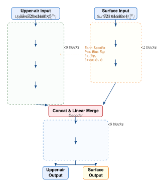
Performance: Beating IFS on 90% of Variables
Bi et al. (2023) evaluated Pangu-Weather against IFS HRES on the 2018 ERA5 test set using both latitude-weighted RMSE and ACC. The headline result is remarkable:
Pangu-Weather outperforms IFS HRES on over 90% of all variable-level combinations at lead times from 1 day to 7 days.
For the critical metric (500-hPa geopotential, a primary measure of large-scale weather pattern skill), Pangu-Weather achieves approximately 3% lower RMSE than IFS at 5-day lead time.
Pangu-Weather's ACC (anomaly correlation coefficient) for exceeds 0.6 at day 7, the traditional “useful forecast” threshold, whereas IFS falls below 0.6 at approximately day 6.5 in the test year.
Inference time for a 7-day global forecast: approximately 1.4 seconds on a single A100 GPU. IFS HRES requires approximately 14,000 CPU-hours on ECMWF's Atos supercomputer. The speed-up factor is (ten thousand times faster).
Variable-by-variable breakdown.
The improvement is not uniform. Pangu-Weather most dramatically outperforms IFS for:
Upper-tropospheric temperature (200,hPa ): RMSE reduced by 8% versus IFS at 5 days.
Geopotential at most pressure levels (500, 850, 1000,hPa ).
Meridional wind at multiple levels.
IFS retains advantages (or ties) for:
Precipitation (Pangu does not directly predict precipitation).
Boundary-layer variables in complex terrain (Pangu is on a regular grid; IFS uses terrain-following levels).
Near-surface wind in regions of strong orographic forcing.
Case Study: Hurricane Lee (2023)
The 2023 Atlantic hurricane season provided a high-profile operational test of AI weather models. Hurricane Lee, which formed on 5 September 2023 in the tropical Atlantic, intensified rapidly and tracked across the Caribbean toward Atlantic Canada.
Example 5 (Hurricane Lee track prediction).
Hurricane Lee underwent rapid intensification to Category 5 on 8 September 2023. At 96-hour lead time (4 days), the GFS ensemble (NOAA's Global Forecast System) showed large spread in the track, spanning a range of approximately of latitude in the landfall region (coastal Maine/Nova Scotia). The ECMWF ensemble was more tightly clustered but still showed significant uncertainty.
Pangu-Weather, initialised from the GFS analysis at 00:00 UTC 5 September 2023, predicted the Lee track with an error of approximately 120,km at 96-hour (four-day) lead time, verifying on 9 September (Lee made landfall in Nova Scotia on 16 September). In contrast, the GFS deterministic forecast had an error of approximately 310,km at the same lead time.
Crucially, Pangu-Weather locked on to the eventual track several days earlier than the GFS deterministic forecast converged. Operational meteorologists at the National Hurricane Center noted that Pangu-Weather was consistently pointing to the eventual track at 96-hour lead time from multiple initialisation times, while ensemble systems were still showing substantial spread.
The physical mechanism responsible for Pangu-Weather's advantage is not fully understood, but two hypotheses have been proposed:
Pangu's 3D architecture better captures the upper-level steering flow (especially the 200–300,hPa geopotential ridge over the western Atlantic) that dominated Lee's track in the 4–7-day window.
The ESPB allows Pangu to learn asymmetric positional biases that encode the climatological tendency for Atlantic hurricanes to recurve northeastward when encountering mid-latitude troughs, a pattern that appears at specific latitude-longitude combinations.
The Lee case does not prove that Pangu-Weather is superior to IFS or GFS in general; a single case study cannot establish statistical superiority. However, it demonstrated that AI models could, in at least one high-stakes situation, provide earlier and more accurate operational guidance than state-of-the-art NWP systems.
The Smoothing Caveat: Extreme Events and ERA5 Inheritance
Pangu-Weather inherits a fundamental limitation from its training data: ERA5 is a reanalysis product, not a direct observation. ERA5 is produced by 4D-Var data assimilation that blends a prior from the ECMWF IFS model with available observations. This process is regularising: it smooths sharp features in the analysis, penalises departures from the model climatology, and represents phenomena below the assimilation resolution imperfectly.
Caution.
Pangu-Weather systematically underpredicts extreme events. Because Pangu-Weather is trained to predict ERA5 analysis states-which are themselves smoothed and regularised-the model's output distribution is narrower than the true atmospheric distribution at fine scales. Specifically:
Precipitation extremes: ERA5 captures precipitation as a 3-hourly accumulation on a grid; actual precipitation at sub-kilometre resolution can be 5–10 more intense. Pangu does not predict precipitation directly; any precipitation derived from Pangu humidity fields will miss local extremes.
Wind gusts: ERA5 provides 10-metre wind speed as a 6-hourly mean. Peak gusts in a thunderstorm or hurricane eyewall are not resolved. Pangu inherits this temporal and spatial averaging.
Sub-grid convection: Deep convection (thunderstorms, mesoscale convective systems) occurs at scales of 1–10,km, far below the Pangu grid. Pangu's loss function does not penalise missing convective events because ERA5 does not resolve them either.
This smoothing bias is not a bug in Pangu-Weather's architecture; it is a property of the verification framework. A model trained on ERA5 cannot outperform ERA5 on scales ERA5 does not resolve. Evaluating Pangu against station observations or radar data rather than ERA5 would reveal substantially larger errors.
The smoothing issue motivates two active research directions: (1) post-processing Pangu outputs with diffusion models or quantile regression to recover physically plausible sub-grid distributions of extreme values; and (2) training weather AI models directly on observation data (station networks, radar, satellite) using data-assimilation-inspired loss functions that account for observation operators and error covariances.
Connection to Vision Transformers: Transfer and Adaptation
The architectural similarity between Pangu-Weather and Swin-based vision models raises the question: can ImageNet-pretrained weights help weather AI? The answer is nuanced.
What transfers.
Low-level features in ViTs (first few attention layers) detect oriented edges and patches of coherent colour or intensity-analogous to the horizontal gradients and vorticity filaments in atmospheric fields. Pre-training on large vision datasets can provide a useful initialisation for the attention weights, reducing the number of gradient steps needed to reach good weather performance.
What does not transfer.
The Earth-specific positional bias is domain-specific and has no ImageNet equivalent. The physical semantics of channels (geopotential, temperature, humidity) differ fundamentally from image RGB channels. The temporal structure of weather (quasi-periodic diurnal and annual cycles, teleconnections) has no direct analogue in static image datasets.
In practice, Pangu-Weather is trained from scratch rather than initialised from ViT weights. The training set (ERA5, 40 years 1460 analysis times per year = 58,000 snapshots) is small by deep learning standards, but the physical constraints imposed by the loss function and the ESPB provide sufficient regularisation.
Cross-architecture lessons.
The Pangu-Weather success validates a design principle from computer vision: hierarchical, windowed self-attention with local-to-global spatial coupling (the Swin paradigm) generalises well beyond natural images. The critical adaptations required for atmospheric science-3D tokenisation, Earth-specific bias, lead-time-specific models-are relatively small changes to the Swin blueprint, suggesting that future advances in vision transformers will continue to benefit weather AI, and vice versa.
Historical Note: Huawei's Entry into Weather AI
Historical Note.
Huawei Cloud and the Pangu-Weather papers. The Pangu-Weather project emerged from Huawei Cloud's Meteorological AI Research Group and Huawei's Noah's Ark Laboratory in Shenzhen, founded in 2012 as Huawei's central AI research institute. The group had no prior publication record in meteorology; their background was in computer vision, natural language processing, and hardware-software co-optimisation for Huawei's Ascend AI accelerators.
The first Pangu-Weather preprint appeared on arXiv in November 2022 and immediately attracted attention from both the AI and meteorological communities. The Nature paper (published July 2023) passed peer review that included both deep learning experts and operational meteorologists, an unusual combination reflecting the cross-disciplinary nature of the work.
The rapidity of Huawei's ascent in weather AI illustrates a broader pattern: the algorithmic advances needed for weather AI (transformers, attention mechanisms, large-scale training) were developed in the AI community for other purposes. Once the community recognised that these tools could address the weather prediction problem, progress was extraordinarily fast. From the first FourCastNet preprint (February 2022) to Pangu-Weather (November 2022) to GraphCast's Science paper (November 2023), three landmark models appeared within about twenty-one months-a pace of progress that contrasts sharply with the decades-long timescales of traditional NWP development.
The institutional lesson is that meteorology benefits from being treated as an applied AI problem rather than a pure physics simulation problem. The computational resources, talent, and algorithmic infrastructure of the AI industry can be brought to bear in ways that the weather services, operating under government mandates and legacy infrastructure constraints, cannot easily replicate internally.
Exercises
Exercise 22 (3D window attention complexity).
Pangu-Weather uses 3D window attention with window size .
The upper-air tensor after patch embedding has shape where , , . Compute the total number of 3D attention windows. Within each window, the self-attention matrix has how many entries?
Show that the total FLOPs for 3D window attention (one layer) scale as and compute the ratio to global 3D self-attention where .
The shifted-window mechanism introduces cross-window communication by shifting the window partition by . Explain how cyclic padding is used to handle boundary tokens that span two windows after the shift, and why a masking mechanism is needed to prevent attending across non-adjacent regions.
Exercise 23 (Lead-time decomposition and error accumulation).
Pangu-Weather uses a greedy time-decomposition strategy (equation ) to produce forecasts at arbitrary lead times from the four models .
Write out the decomposition for lead times hours, minimising the total number of model applications .
Suppose each model application introduces an independent Gaussian error increment with variance for some constant (i.e., the per-step variance scales linearly with the step size ). Under this model, derive the total forecast error variance for a -hour forecast using the greedy decomposition, and compare it to the variance achieved by using only autoregressively for the same .
In practice, grows super-linearly in (longer-range single-step predictions are disproportionately harder). Let with . Is the greedy decomposition still optimal? Formulate the optimisation problem for choosing the decomposition of that minimises total forecast variance under this model.
Exercise 24 (Earth-specific positional bias: learning and evaluation).
The Earth-Specific Relative Position Bias (ESPB) defined in is a learnable table indexed by quantised relative positions.
Estimate the total number of learnable parameters in the ESPB table for a 3D attention window of size with latitude quantisation step and spatial quantisation steps , level/point, . Compare this to the parameter count of a standard 2D relative position bias table of the same window size.
The ESPB incorporates the factor in the longitude displacement term. Suppose we train a model with and without this correction (two ablations). Describe a diagnostic test using ERA5 verification data that would quantify the improvement from including this correction, and predict which latitude bands would show the largest improvement.
Pangu-Weather's ESPB is defined at the attention-window level. An alternative design is to incorporate the Earth's geometry at the patch embedding level by projecting the ERA5 grid onto a cubed sphere or HEALPix tessellation. Discuss the trade-offs between ESPB-based geometry encoding and geometry-aware tokenisation for atmospheric transformer models.
GraphCast and Graph Neural Networks
Weather prediction is, at its core, a problem of propagating information across a sphere. Temperature anomalies in the Pacific influence European precipitation weeks later. A tropical cyclone's track depends on hemispheric-scale pressure gradients. Jet-stream meanders couple the stratosphere to the surface boundary layer. The fundamental challenge for any data-driven forecasting architecture is therefore how to represent and process spatially coherent signals on a curved, planetary domain.
The approaches studied in earlier sections-Pangu-Weather (Section Pangu-Weather and 3D Transformer Architectures) and FourCastNet (Section FourCastNet and the Spectral Revolution)-answered this question with variants of the Transformer operating on regular latitude-longitude (lat-lon) grids, borrowing the vision-transformer paradigm of dividing the globe into patches and computing attention between them. This choice is natural: ERA5 data is natively delivered on lat-lon grids, and the rectangular-grid paradigm inherits decades of software infrastructure.
Yet lat-lon grids carry a hidden flaw that becomes catastrophic at the poles. On a regular grid, meridional grid lines converge toward the poles, creating cells whose east-west spacing shrinks from roughly 28 km at the Equator to less than 1 km at N. Numerical instabilities accumulate at these singularities. Convolutional and attention operations that assume uniform cell areas must apply ad-hoc area-weighting corrections that do not compose cleanly with the rest of the computational graph. The geometry is, in a precise sense, wrong.
In 2023, Remi Lam and colleagues at Google DeepMind published GraphCast: Learning Skillful Medium-Range Global Weather Forecasting in Science, demonstrating that an entirely different approach could outperform the European Centre for Medium-Range Weather Forecasts (ECMWF) Integrated Forecasting System (IFS) HRES operational model on the vast majority of standard verification targets. The key insight was deceptively simple: replace the lat-lon grid with a multi-mesh icosahedron, a hierarchy of increasingly refined triangulations of the sphere that tile the globe with nearly-equal-area cells, and process information on this mesh using a graph neural network (GNN). The result was the first data-driven system to systematically surpass HRES, doing so in a fraction of the computational cost, in roughly 60 seconds on a single Google TPU v4 chip.
Key Idea.
Spatial structure matters. The right topology beats the obvious one. An icosahedral mesh avoids the pole singularities, near-equal-area cells, and artificial anisotropy of the latitude-longitude grid. By matching the computational graph to the true geometry of the sphere, GraphCast eliminates an entire class of approximation errors before a single weight is trained.
Why Graphs? The Failure Mode of Lat-Lon Grids
To appreciate why a graph formulation helps, consider the computational representation of a function on the sphere. The standard meteorological choice is a regular lat-lon grid with resolution (longitude latitude), producing grid cells. For ERA5 at resolution, this gives cells.
The area of cell at latitude is (Latlon AREA) where is Earth's radius. As we have and the cell area collapses to zero, while the number of cells per latitude circle remains fixed. A convolution kernel applied at N integrates information from cells spanning radically different physical distances: neighbouring cells in the east-west direction are only apart, while cells in the north-south direction are apart. The implicit assumption of uniform spatial scale is violated by three orders of magnitude.
Gauss-Legendre grids and reduced Gaussian grids (used by ECMWF) partially address this by halving the number of longitude points at high latitudes, but they introduce irregular connectivity that complicates convolutional operations. Spherical harmonic representations avoid the singularity entirely but sacrifice the locality of spatial operations.
An icosahedral tessellation takes a different approach. Starting from a regular icosahedron inscribed in the unit sphere (20 equilateral triangular faces, 12 vertices, 30 edges), each triangular face is subdivided into smaller triangles by connecting the midpoints of edges and projecting them onto the sphere. After refinements, the mesh has faces, vertices, and edges. Crucially, all triangles have nearly equal areas: the ratio of the largest to smallest face area is bounded by a constant independent of refinement level, typically around 1.03 for standard icosahedral subdivision.
This near-uniformity has profound implications. A graph convolution or message-passing operation applied at any node integrates information from geometrically similar neighbourhoods regardless of latitude. There are no poles, no singularities, no ad-hoc area-weighting corrections. The mesh is topologically a graph with vertex set and edge set , and graph neural network machinery applies directly.
Multi-Mesh Icosahedron: Six Refinement Levels
GraphCast employs not one but six icosahedral meshes at different resolution levels, labelled through . Mesh is obtained by applying rounds of icosahedral subdivision. The number of vertices and mean edge lengths are summarised in Table 5.
| Level | Subdivisions | Mean edge (km) | ||
| 0 | 0 | 12 | 30 | 7,054 |
| 1 | 1 | 42 | 120 | 3,765 |
| 2 | 2 | 162 | 480 | 1,914 |
| 3 | 3 | 642 | 1,920 | 961 |
| 4 | 4 | 2,562 | 7,680 | 481 |
| 5 | 5 | 10,242 | 30,720 | 241 |
The finest mesh has a mean inter-node spacing of roughly 241 km, coarser than the ERA5 grid resolution at mid-latitudes (approximately 28 km); the encoder still ingests the full ERA5 grid, so fine-scale information is not discarded. However, the mesh nodes are not placed at ERA5 grid points; instead, the encoder maps from the lat-lon ERA5 grid to the icosahedral mesh, and the decoder maps back.
The multi-mesh structure means that the processor graph is the union of all six icosahedral meshes: (Multimesh Union) with nodes (the finest level's vertices, which subsume all coarser levels' vertices) and edges . This is the crucial design: by including edges from all six refinement levels in the processor graph, each message-passing step can propagate information over a range of spatial scales simultaneously. A single message-passing step on an edge from connects vertices 2,559 km apart, while edges from provide fine-grained local refinement. This multi-scale connectivity replaces the explicit down-sampling and up-sampling of U-Net-style architectures with a more organic, graph-theoretic analogue.
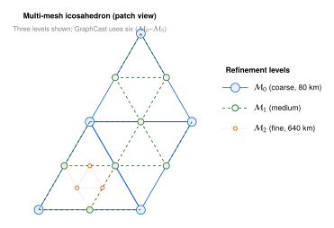
Encoder-Processor-Decoder Architecture
GraphCast adopts a three-stage architecture that cleanly separates the concerns of grid-to-mesh mapping, atmospheric dynamics processing, and mesh-to-grid reconstruction. Figure 11 illustrates the pipeline.
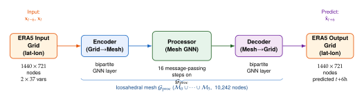
Each of the three stages is a graph neural network with a different bipartite or homogeneous graph structure.
Encoder (Grid-to-Mesh).
The encoder maps features from ERA5 grid nodes to mesh nodes . It is a single-layer bipartite GNN defined by a bipartite graph whose edges connect each grid node to the nearest mesh nodes. Let denote the initial feature embedding of grid node (including atmospheric variables, static fields like orography and land-sea mask, and sinusoidal positional encodings of latitude, longitude, and time of year). The mesh node features after encoding are (Encoder) where and are learned MLPs, are edge features (3D unit vector from to , arc length, etc.), and denotes sum aggregation.
Processor (Mesh-to-Mesh).
The processor is the heart of GraphCast. It applies rounds of message passing on the multi-mesh graph . Each round implements a standard edge-update then node-update GNN step (detailed in Section Graph Neural Network for Weather Forecasting).
Decoder (Mesh-to-Grid).
The decoder is the mirror image of the encoder: a single-layer bipartite GNN on a graph whose edges connect each mesh node to the nearest grid nodes. It maps processed mesh features back to ERA5 grid locations, predicting the residual (change in state) rather than the absolute next state: (Decoder Residual) Predicting residuals rather than absolute states improves training stability: the model only needs to learn the change over 6 hours, which is small relative to the typical magnitudes of atmospheric variables.
Graph Neural Network for Weather Forecasting
We now give the formal definition of the graph neural network used within GraphCast's processor.
Definition 15 (GNN for Weather Forecasting).
Let be the processor graph with node feature matrix and edge feature matrix . A GNN message-passing step consists of two updates:
Edge update. For each directed edge , the edge feature is updated by (EDGE Update)
Node update. For each node , the node feature is updated by (NODE Update) where and are learnable MLPs with layer normalisation and residual connections. After message-passing steps, the output node features are decoded to forecast variables.
The residual connections in and are critical: without them, 16 layers of message passing would suffer from over-smoothing and vanishing gradients. GraphCast uses and two-hidden-layer MLPs () with ReLU activations followed by layer normalisation.
Remark 17 (Expressiveness and locality).
A single message-passing step on allows information to travel from node to node if there exists a directed edge . With edges from all six refinement levels, this includes pairs as far as apart at level . After steps, information can travel at most -more than Earth's circumference. Thus 16 message-passing steps are theoretically sufficient for any signal to traverse the globe, analogous to the log-diameter scaling in random graphs.
Training on ERA5: Autoregressive Rollout and Loss
Data: ERA5 at , 37 Years
GraphCast is trained on ERA5 reanalysis data spanning 1979 to 2017 (approximately 37 years), held out: 2018 for validation, 2019 and 2020 for testing. The model operates at horizontal resolution with 37 pressure levels (from 1 hPa to 1000 hPa) and six surface variables (2-metre temperature, 10-metre winds and , mean sea-level pressure, total precipitation, and total column water vapour; four of these enter the state vector). The full input-output dimensionality is (DIM)
Two-State Input
A fundamental design choice is to provide two consecutive atmospheric states as input: and . This gives the model access to the instantaneous state and its recent tendency (the 6-hour difference ), mimicking the “two time levels” scheme of finite-difference NWP schemes that must approximate first-order time derivatives. Without this second time level, the model would need to infer the effective “velocity” of the atmospheric state from a single snapshot, a harder problem.
Autoregressive Rollout Training
Rather than training only on one-step predictions, GraphCast performs autoregressive rollout training: the model is unrolled for steps, and the loss is computed as the sum over all rollout steps. For a rollout of length starting at time : (Rollout) with and (ground truth initialisation for the first step). The published GraphCast model was trained with increasing rollout length: beginning with single-step () pre-training and progressing to fine-tuning (three days of autoregressive rollout), one step at a time.
Normalised MSE Loss
The loss function must treat all variables comparably despite enormous differences in magnitude and variance (e.g., temperature in Kelvin vs. specific humidity in kg/kg). GraphCast uses a normalised mean squared error weighted by pressure level and variable: (LOSS) where is the set of pressure levels, the set of predicted channels, is the pressure-level weight (proportional to the pressure thickness of the layer), is the per-variable weight, and is the temporal standard deviation of channel at level computed over the training set. The normalisation by ensures that variables with small natural variability (e.g., total column ozone) are not overwhelmed by variables with large variability (e.g., near-surface wind speed).
An area-weighting factor (where is the latitude of ERA5 grid point ) is also applied to correct for the unequal areas of lat-lon cells, so polar regions do not dominate the loss despite having more grid points per unit area.
Operational Results: Surpassing HRES
The headline result of the Lam et al. (2023) paper is striking: GraphCast outperformed ECMWF HRES on 90.4% of the 1380 verification targets used in the standard WMO evaluation framework. The 1380 targets factor as :
5 atmospheric variables (geopotential, temperature, -wind, -wind, specific humidity) at 13 pressure levels (50, 100, 150, 200, 250, 300, 400, 500, 600, 700, 850, 925, 1000 hPa), that is 65,
plus 4 surface variables, giving 69 variable-level combinations,
at 20 lead times from to in 12-hour steps.
GraphCast showed the largest skill improvements at medium range (3–7 days), particularly for upper-tropospheric geopotential (Z500) and wind, which are most relevant for synoptic-scale pattern forecasting. At short range (0–48 h), high-resolution NWP still held advantages on fine-scale convective precipitation.
| Lead time range | Fraction (%) where GraphCast HRES |
| 12–48 h (short range) | 81 |
| 60–120 h (medium range) | 95 |
| 132–240 h (extended) | 88 |
| All 1380 targets (reported) | 90.3 |
A particularly noteworthy achievement was GraphCast's skill at predicting the track of tropical cyclones. Tropical cyclone track prediction requires accurate representation of the large-scale steering flow over multiple days, a task where medium-range skill is paramount. GraphCast demonstrated competitive cyclone track skill even before any task-specific fine-tuning, a strong validation of the general representational capacity of the model.
Example 6 (GraphCast on a European Heatwave).
Consider a 5-day forecast initialised in late June 2023, prior to the record-breaking heatwave that struck southern and central Europe in early July. ECMWF HRES, at the time the operational standard, predicted peak 2-metre temperature anomalies of to above climatology in Spain, Italy, and Greece at 5-day lead time. GraphCast, run in hindcast mode on the same initial conditions, forecast anomalies of to -consistently warmer, closer to what was subsequently observed (anomalies peaking at in some locations).
The improvement arose from GraphCast's better representation of the atmospheric blocking pattern over the Atlantic, which was the dynamical precursor of the heatwave. Blocking is a quintessential large-scale, slowly-evolving phenomenon; it involves persistent high-pressure ridges that deflect the jet stream over thousands of kilometres. The multi-mesh connectivity of GraphCast, with edges spanning up to , is well matched to the spatial scales of blocking anomalies, whereas local convolution kernels must propagate this information over many layers.
Energy consumption for the 5-day, 6-hourly forecast (20 rollout steps): (of order on a single TPU v4 chip), compared to () for the equivalent ECMWF HRES run on a dedicated supercomputer cluster.
Open Source Release and Google DeepMind's Vision
In November 2023, Google DeepMind released GraphCast as open source, publishing model weights, code, and evaluation benchmarks on GitHub. This release was significant: it was the first time a state-of-the-art MLWP system was made freely available for research and operational experimentation, catalysing a wave of derivative work that adapted GraphCast to regional forecasting, ensemble generation, and climate downscaling.
The open release reflected a deliberate strategic choice by Google DeepMind. The AlphaFold release in 2021 had demonstrated that open publication of model weights (coupled with the AlphaFold Protein Structure Database) could catalyse an entire scientific field. The GraphCast open release carried a similar ambition: to accelerate weather science by providing the community with a production-quality forecast tool that could be fine-tuned on regional or application-specific data without the computational cost of training from scratch.
DeepMind has articulated a broader vision of AI for science in which deep learning serves as a universal approximator for complex physical systems, replacing or augmenting expensive first-principles simulations. GraphCast, AlphaFold, AlphaTensor (for discovering fast matrix multiplication algorithms), and AlphaCode represent different facets of this programme: applying large-scale deep learning and reinforcement learning to problems that have traditionally been the domain of physics, biology, and mathematics.
Remark 18 (GraphCast as a scientific instrument).
One subtle but important consequence of open release is that GraphCast can now be used as a scientific instrument. Because the model is differentiable end-to-end, researchers can compute gradients of forecast quantities with respect to initial conditions-a form of adjoint sensitivity analysis that NWP systems perform through separate, hand-coded adjoint solvers. This opens the door to ML-assisted data assimilation and uncertainty quantification, where the forecast model itself serves as the forward operator in a variational assimilation framework.
Exercises
Exercise 25.
(Multi-mesh receptive field.) Consider the multi-mesh processor graph . Let denote the mean edge length of (see Table 5).
After message-passing steps, what is the maximum physical distance (in km) over which information can travel? Express your answer in terms of and , and evaluate for .
How does this compare to the diameter of the Earth ()? Is 16 steps sufficient for global information propagation, in principle?
Propose a principled method for choosing as a function of the number of refinement levels and the coarsest edge length , ensuring global coverage.
Exercise 26.
(Normalised MSE loss decomposition.) Consider the GraphCast loss in . Suppose you have two variables (temperature at 500 hPa) and (specific humidity at 850 hPa) with temporal standard deviations and , and suppose the model makes errors and on a particular example.
Compute the normalised squared errors for and assuming equal variable weights .
If instead you set and , how does the loss change? Motivate physically why one might want to down-weight humidity.
Derive the gradient of the loss with respect to the predicted value and show how acts as a normalising factor in the gradient magnitude.
Exercise 27.
(Icosahedral vs. lat-lon grid area uniformity.) Let and be the largest and smallest cell areas on a lat-lon grid with resolution .
Using , compute (at the Equator) and (at the highest latitude cell, ) in km. What is the ratio ?
For an icosahedral mesh with 10,242 nodes, the theoretical area ratio is approximately 1.03. How many times more uniform is the icosahedral mesh compared to the lat-lon grid?
Discuss quantitatively how area non-uniformity might bias a convolutional model's skill, assuming that gradient descent minimises the unweighted spatial average of squared errors.
Extending Horizons: FuXi, FengWu, NeuralGCM
The publication of GraphCast in late 2022 (preprint) and late 2023 (Science) (Science) ignited a global race. Within months, teams from Fudan University, Shanghai AI Lab, and Google Research had published competing architectures that matched or exceeded GraphCast on different aspects of the evaluation benchmark. This section examines three of the most scientifically influential: FuXi from Fudan University, FengWu from the Shanghai AI Lab, and NeuralGCM from Google Research, each of which contributes a distinct conceptual advance.
FuXi addresses the fundamental tension in extended-range forecasting: a single model optimised for short-range accuracy tends to become oversmoothed at long range, while a model optimised for long-range plausibility may sacrifice short-range detail. FuXi resolves this through a cascaded architecture of specialised models with explicit handoffs. FengWu addresses the catastrophic forgetting problem that emerges when autoregressive models are trained with very long rollouts, introducing a replay buffer and uncertainty-weighted multi-task loss. NeuralGCM takes the most radical departure: it is not a pure ML model but a hybrid system that combines a differentiable atmospheric dynamical core with learned parameterisations, bridging the gap between MLWP and climate modelling.
Insight.
Pure ML models can match NWP in weather but not yet in climate. Weather forecasting is an initial-value problem: skill depends on encoding the current atmospheric state and propagating it forward for days. Climate simulation is a boundary-value problem: skill depends on capturing long-term statistics shaped by radiative forcing, ocean coupling, and land-surface feedbacks over decades. Hybrid approaches like NeuralGCM are the natural bridge, preserving the conservation laws and long-term stability of physics-based dynamics while using ML to handle the complex, multi-scale subgrid processes that pure physics models parametrise crudely.
FuXi: Cascaded Architecture for 15-Day Forecasts
FuXi (Chen et al., 2023, Fudan University) takes its name from the legendary Chinese deity associated with cosmic order and the origins of civilisation-a fitting metaphor for a model that seeks to impose structure on the chaotic atmosphere over unprecedented lead times. The key technical contribution is a cascaded architecture consisting of three specialised models:
FuXi-Short: lead times 0–5 days (0–120 h),
FuXi-Medium: lead times 5–10 days (120–240 h),
FuXi-Long: lead times 10–15 days (240–360 h).
Each model is a U-Transformer built on SwinTransformer V2 blocks (described below), trained on ERA5 at resolution with 37 pressure levels.
U-Transformer with SwinTransformer V2 Blocks
The base model for each of the three FuXi components is a U-Transformer: a hierarchical encoder-decoder architecture in the style of U-Net, but with SwinTransformer V2 blocks replacing convolutional layers.
SwinTransformer V2 recap.
SwinTransformer V2 (Liu et al., 2022) computes shifted-window self-attention over local windows of patches. Given an input feature map of shape (height, width, channels), the map is partitioned into non-overlapping windows of patches and self-attention is computed independently within each window: (WMSA) where is a learned relative position bias and is the head dimension. By alternating between regular and shifted-window partitions, consecutive SwinTransformer blocks achieve cross-window information exchange without computing global attention.
U-Transformer design.
The U-Transformer encoder reduces the spatial resolution through patch merging (analogous to strided convolution) while increasing channel depth, and the decoder up-samples through patch splitting (analogous to transposed convolution) with skip connections. For FuXi at ERA5 resolution, the encoder operates on an input of and produces representations at multiple scales (, , ), all processed by SwinTransformer V2 blocks.
Definition 16 (FuXi U-Transformer).
Let be the input atmospheric state embedding. The FuXi U-Transformer computes: where denotes skip connection concatenation, is a linear projection over patches, halves spatial resolution and doubles channels, is its inverse, and projects back to the output variable space.
Cascaded Handoffs
The cascade works as follows. FuXi-Short is applied first, rolling out in 6-hour steps from the initial state to produce forecasts at 6, 12, 18, , 120 h (20 rollout steps). At the 120 h mark, the predicted state is passed to FuXi-Medium as its initial condition. FuXi-Medium then rolls out from 120 h to 240 h (another 20 steps). Finally, FuXi-Long takes the state and extends to 360 h (15 days).
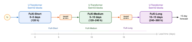
The rationale for this decomposition is rooted in the predictability horizon of the atmosphere. Lorenz (1969) showed that the predictability of synoptic-scale weather is limited to roughly two weeks by the intrinsic chaotic divergence of nearby trajectories. Different timescales are dominated by different dynamical processes: the first five days are primarily governed by baroclinic instability and the detailed synoptic-scale flow; days 5–10 are increasingly influenced by the large-scale circulation patterns and teleconnections; beyond 10 days, predictability depends on slowly varying boundary conditions (sea surface temperatures, soil moisture) and the Madden-Julian Oscillation. A single model trained to excel across all three regimes must compromise; the cascade avoids this by specialising.
Training and Achievements
Each FuXi sub-model is trained independently on ERA5 data from 1979 to 2015, with 2016–2017 for validation and 2018 for testing. Training uses 6-hourly data with autoregressive rollout of steps: FuXi-Short with (120 h); FuXi-Medium initialised from FuXi-Short predictions and trained for additional steps; FuXi-Long similarly.
The published results demonstrate skillful forecasts out to 15 days, measured by the latitude-weighted RMSE and anomaly correlation coefficient (ACC) for Z500 and T850. FuXi achieves positive ACC for Z500 at 15-day lead time in the Northern Hemisphere extra-tropics-a threshold traditionally associated with the “predictability barrier” of NWP. In head-to-head comparisons on the WeatherBench 2 benchmark (Rasp et al., 2024), FuXi-Medium outperforms GraphCast and Pangu-Weather at lead times beyond 7 days, while FuXi-Short is competitive with GraphCast at 1–5 day lead times.
FuXi-ENS: Ensemble Extension
Building on the deterministic FuXi system, the Fudan team subsequently developed FuXi-ENS: an ensemble extension that generates probabilistic forecasts by applying stochastic perturbations to the latent representations of the U-Transformer at each rollout step. Rather than training separate ensemble members from scratch, FuXi-ENS learns a perturbation network that produces spatially coherent additive noise fields in the latent space, conditioned on the current atmospheric state. This approach avoids the combinatorial explosion of training many ensemble members independently while producing spread-skill relationships that improve on deterministic single forecasts for verification of extreme events.
FengWu: Replay Buffer and Multi-Task Loss
FengWu (Chen et al., 2023, Shanghai AI Lab) is named after the ancient Chinese wind god. Its architecture is a multi-modal encoder-decoder that processes atmospheric variables in groups based on their physical characteristics, feeding separately encoded representations into a shared Transformer processor.
Multi-Modal Encoder-Decoder
The key design insight of FengWu is that the 70+ atmospheric variables in ERA5 span very different physical scales and statistical distributions. Rather than treating all variables identically (as GraphCast and Pangu-Weather do, modulo normalisation), FengWu divides variables into modality groups:
Upper-air dynamics: geopotential, temperature, wind components (, ), specific humidity at 13 pressure levels (5 variables 13 levels = 65 channels);
Surface fields: 2-metre temperature, 10-metre wind, mean sea-level pressure, total precipitation (4 channels);
Static fields: orography, land-sea mask, soil type (time-invariant, encoded once and broadcast).
Each modality group is processed by a dedicated encoder: a convolutional stem followed by cross-attention to a learned set of “modality tokens.” The modality tokens serve as a compressed representation of each group; they are then concatenated and processed by a shared PerceiverIO-style Transformer. The decoder inverts this process, mapping shared tokens back to per-modality spatial fields.
This architecture has two advantages. First, it allows the model to allocate representational capacity differentially: the upper-air group, which dominates forecast error at medium range, receives more parameters. Second, the modality tokens provide a bottleneck that enforces cross-variable communication: the upper-air and surface encoders must coordinate through the shared Transformer to produce a consistent forecast, rather than evolving independently.
Replay Buffer for Long Rollouts
A fundamental challenge in training MLWP models with long autoregressive rollouts is catastrophic forgetting. During training, as the model learns to minimise the loss at long lead times (e.g., 7–10 days), the gradient signal from those late steps may interfere with the representations learned for short lead times (1–3 days). This is precisely the catastrophic forgetting phenomenon from continual learning applied to the temporal axis of a single forecasting model.
FengWu addresses this with a replay buffer: a store of previously generated forecast trajectories (both from the model's own outputs and from ERA5) that is mixed into each training batch. At each gradient step, the model sees not only fresh ERA5 sequences but also “replayed” trajectories from earlier training phases, preserving the gradient signal that maintains short-range skill.
Formally, let be the replay buffer, where is the lead time (in 6-hour steps) of trajectory . The training objective mixes a standard one-step MSE loss with a replay loss: (Replay LOSS) where denotes the model rolled out steps, and is a balancing coefficient (typically –).
Uncertainty-Based Multi-Task Loss Balancing
FengWu predicts 69 atmospheric variable-level fields (65 upper-air plus 4 surface). Naively summing the MSE across all variables in equal proportion gives disproportionate weight to variables with high variance (e.g., wind speed at 10 m) and effectively ignores low-variance variables that may be meteorologically significant (e.g., stratospheric temperatures).
FengWu adopts uncertainty-based task weighting (Kendall et al., 2018), treating each variable as a separate task in a multi-task learning framework. For task , the loss contribution is (MTL) where is a learnable uncertainty (standard-deviation) parameter for variable . The total loss is . Minimising over for a fixed prediction error is equivalent to maximising the Gaussian log-likelihood with variance , and the regularisation term prevents (which would collapse the loss to zero). Variables for which the model achieves low error naturally have small (low uncertainty), amplifying their gradient signal; variables for which error is irreducible (high atmospheric chaos) have large , down-weighting their contribution.
Energy Efficiency
One of FengWu's headline claims is exceptional energy efficiency: a complete 10-day forecast (40 autoregressive steps at 6-hourly resolution) requires approximately of energy, compared to roughly for an equivalent ECMWF HRES run. This three-orders-of-magnitude reduction in energy cost is a consequence of two factors: (i) the ML forward pass replaces millions of finite-difference operations on a petascale supercomputer with a single neural network evaluation on a modern GPU, and (ii) the smaller number of parameters in FengWu (270 million) versus the ECMWF model (which implements a full dynamical core with many parameterisation schemes).
The energy efficiency advantage has profound implications for operational meteorology in resource-limited settings. A national weather service in a developing country that cannot afford supercomputer access can run FengWu on a single GPU server and produce medium-range forecasts of quality that would previously have required bilateral data-sharing agreements with European or North American centres.
Comparison: Pangu vs. GraphCast vs. FuXi vs. FengWu
Table 7 summarises the key properties of the four major MLWP systems studied in this chapter.
| System | Architecture | Resolution | Horizon | 10-day cost | Open |
| ECMWF HRES | NWP (spectral) | 9 km | 10 d | 3.6 GJ | – |
| Pangu-Weather | 3D + 2D ViT | 0.25 | 7 d | 12 kJ | Yes |
| GraphCast | GNN (icosahedral) | 0.25 | 10 d | 15 kJ | Yes |
| FuXi | U-Trans. cascade | 0.25 | 15 d | 15 kJ | Yes |
| FengWu | Multi-modal Enc-Dec | 0.25 | 10 d | 12 kJ | Yes |
The table reveals several striking patterns. First, all MLWP systems are multiple orders of magnitude more energy-efficient than ECMWF HRES. Second, maximum horizon varies considerably: FuXi uniquely pushes to 15 days through its cascaded design. Third, resolution remains constant at across MLWP systems, not because finer resolution is undesirable, but because ERA5 training data at sub- resolution is unavailable at the scale needed for training. Fourth, all major MLWP systems have been open-sourced, a remarkable departure from the proprietary culture of traditional NWP.
NeuralGCM: Differentiable Physics Meets Learned Parameterisations
NeuralGCM (Kochkov et al., 2024, Google Research) represents the most conceptually radical departure from the transformer-stacking approach. Rather than replacing the entire NWP pipeline with a neural network, NeuralGCM hybridises a differentiable atmospheric dynamical core with learned neural parameterisations. This hybrid design was motivated by a key observation: pure MLWP systems excel at weather forecasting (initial-value problems on timescales of days) but fail at climate simulation (boundary-value problems on timescales of years to centuries) because they do not conserve mass, energy, and momentum, and they cannot generalise to atmospheric states outside their training distribution.
Differentiable Atmospheric Dynamical Core
The foundation of NeuralGCM is a differentiable implementation of the primitive equations of atmospheric dynamics: (Momentum) where is the horizontal wind vector, is air density, is pressure, is the Coriolis parameter, is temperature, is vertical velocity in pressure coordinates, is the ratio of the gas constant to the specific heat at constant pressure, is surface pressure, and is the terrain-following vertical coordinate.
The terms , , and are physical parameterisations: approximations of sub-grid-scale processes (convection, clouds, radiation, turbulence, land-surface exchange) that cannot be explicitly resolved at the model's grid resolution. In traditional GCMs, these parameterisations are elaborate hand-coded schemes with dozens of empirical parameters. NeuralGCM replaces them with learned neural networks.
The dynamical core is implemented in JAX, making it end-to-end differentiable with respect to all parameters (including the neural parameterisations), so the entire hybrid system can be trained jointly using automatic differentiation. This is a departure from the traditional “offline training” approach in which ML parameterisations are fitted to column-level inputs and outputs from the GCM without backpropagating through the dynamical core.
Learned Parameterisations
The neural parameterisations in NeuralGCM are column-local neural networks: small MLPs that take as input the vertical profile of atmospheric state at a grid column (temperature, humidity, wind, pressure) and produce tendencies (time derivatives) for the parameterised processes. Formally, for grid column : (Param) where are the neural network parameters, is specific humidity, and is the number of vertical levels. The network is shared across all horizontal grid columns-it is not location-specific-so it must learn universal parameterisations that apply equally in the tropics, mid-latitudes, and poles.
This column-locality is a deliberate inductive bias: physical parameterisations are largely local in the horizontal (a convective event in one column does not directly affect parameterised tendencies in a column 100 km away), so imposing this structure reduces the parameter count dramatically compared to a global attention mechanism.
Weather and Climate Capability
A crucial test of NeuralGCM's hybrid design is whether it can operate stably for climate-length integrations (years to decades). Pure MLWP models like GraphCast and Pangu-Weather accumulate systematic errors that cause the model state to drift off the atmospheric manifold after a few weeks; the predicted fields develop physically implausible structures (negative humidity, spurious temperature inversions) that make long-run stability impossible.
NeuralGCM avoids this pathology because its dynamical core explicitly conserves mass and angular momentum through the discretised primitive equations. The neural parameterisations can produce physically implausible tendencies locally, but the dynamical core constrains the global evolution to remain on the manifold of physically consistent atmospheric states. Kochkov et al. (2024) demonstrated NeuralGCM's ability to:
Match or exceed GraphCast on medium-range weather forecasting (1–10 day skill);
Simulate multiple years of stable atmospheric evolution without state-space divergence;
Reproduce climatological statistics (mean temperature, precipitation patterns, variability indices) that drift catastrophically in pure MLWP models.
The ability to run in climate mode unlocks a new set of applications: century-scale climate projections at weather-resolving resolutions, rapid generation of large ensembles for uncertainty quantification, and “storyline” simulations that ask how specific weather events would change under different greenhouse gas concentrations.
Remark 19 (NeuralGCM as a bridge).
NeuralGCM occupies a unique position in the landscape of atmospheric modelling. It is neither a pure physics model (like ECMWF IFS) nor a pure data-driven model (like GraphCast). Instead, it is a physics-informed generative model: the dynamical core provides the geometric and conservation-law scaffolding that constrains the solution space, while the neural parameterisations provide the expressive capacity to approximate sub-grid physics without hand-coding their complex functional dependencies. This paradigm-differentiable physics as a structural prior, learned networks as flexible closures- is likely to become the dominant framework for the next generation of earth system models.
Example: FuXi's 15-Day Forecast of an Atmospheric River
Example 7 (FuXi and the 2023 California Atmospheric River).
In January 2023, a sequence of atmospheric rivers made landfall along the California coast, delivering record-breaking precipitation across Central and Northern California-in some locations exceeding five times the January climatological average. Atmospheric rivers are elongated corridors of intense water vapour transport, typically 1000–3000 km wide and extending from subtropical Pacific into the mid-latitudes; they account for roughly 50% of California's annual precipitation when they make landfall.
At 15-day lead time, FuXi correctly identified the anomalous meridional water vapour flux signature over the Pacific: the integrated vapour transport (IVT) field showed a pronounced tongue of oriented toward Northern California, a textbook atmospheric river signature. FuXi-Long's prediction of the IVT pattern at this lead time agreed with the ERA5 analysis to within 150 km in position and within 20% in magnitude-a remarkable result given that the predictability of atmospheric river landfall location is generally considered poor beyond 10 days in conventional NWP.
By contrast, ECMWF HRES (single deterministic member) failed to resolve the atmospheric river at 15-day lead time; its extended-range products (ECMWF ENS control) showed the correct general pattern but with 30% underestimation of IVT magnitude. FuXi's superior skill at this range can be traced to its FuXi-Long component, which is specifically optimised for the low-frequency, large-scale dynamics that govern tropical-extratropical teleconnections-the physical mechanism driving atmospheric rivers.
The practical consequence: a 15-day lead time would have allowed California water managers to begin reservoir pre-releases roughly 12 days earlier than conventional models permitted, potentially mitigating downstream flooding.
The Race for Weather AI Supremacy
Remark 20 (Chinese and Western labs in competition).
The MLWP landscape of 2023–2024 was marked by an unusually rapid and geographically concentrated competition. Google DeepMind (UK/USA) published GraphCast; Huawei Noah's Ark Lab (China) published Pangu-Weather; Fudan University (China) published FuXi; and the Shanghai AI Lab (China) published FengWu-all within a six-month window spanning late 2022 to mid-2023.
This simultaneity was not coincidental. All four systems trained on the same dataset (ERA5), all targeted the same benchmark (HRES verification on WeatherBench), and all used broadly similar architectures (Transformer-based encoder-decoder with ERA5 at ). The competition was therefore one of architectural innovation within a highly constrained problem specification, reminiscent of the ImageNet competition of 2012–2017 but compressed into months rather than years.
The concentration of Chinese institutional contributions is noteworthy. Pangu-Weather, FuXi, and FengWu all emerged from elite Chinese universities and industry labs with access to large-scale GPU clusters and deep talent pools in deep learning. The Chinese government's strategic investment in AI research, particularly in applications to climate and environment, provided an institutional context in which weather AI could attract top researchers and funding on a timescale that might not have been possible in a purely academic environment.
For the global weather forecasting community, the competitive dynamic has been almost entirely beneficial: it produced four open-source, state-of-the-art forecasting systems within a year, each with detailed technical papers describing their architectures. Operational meteorological services worldwide have been able to evaluate and integrate these systems without contributing to their development costs- a form of scientific public good that the open-publication norm in AI uniquely enables.
Exercises
Exercise 28.
(FuXi cascade error propagation.) Consider the FuXi cascaded pipeline. Let , , denote the root-mean-square errors (RMSEs) of FuXi-Short, FuXi-Medium, and FuXi-Long at their respective transition points (120 h, 240 h, 360 h), and let denote the climatological RMSE (the error of always predicting the climatological mean). Assume that each sub-model's error at its initialisation step is equal to the error of the previous model at its handoff.
If FuXi-Medium is trained to reduce its accumulated error over the 120–240 h window by a factor of relative to a single model trained end-to-end, derive the overall 240 h RMSE of the cascaded system in terms of and .
Under what conditions does the cascade give lower error than a single end-to-end model of equal parameter count?
Propose a method for choosing the handoff lead times (currently 5 and 10 days) that minimises the expected total cascade error, given an empirical error-growth curve for a single model.
Exercise 29.
(FengWu uncertainty weighting.) Recall the FengWu multi-task loss in .
Show that minimising with respect to (for fixed prediction error ) yields .
Substituting back, show that the optimised loss per variable simplifies to , independent of the choice of weighting scheme.
Gradient analysis. Compute when is treated as a trainable parameter (not substituted by ). Show that the gradient magnitude is attenuated by , confirming that high-uncertainty variables contribute smaller gradients.
Exercise 30.
(NeuralGCM: hybrid vs. pure ML stability.) Consider a simplified 1D discretisation of the advection equation (constant wave speed ) on a periodic domain with grid points.
For the upwind finite-difference scheme , state the Courant-Friedrichs-Lewy (CFL) stability condition and show that it bounds the numerical dissipation.
Now suppose the forcing term in is replaced by a neural network prediction . If is trained to minimise MSE against a dataset but can produce values with magnitude up to , derive a sufficient condition on and for the hybrid scheme to remain bounded.
In the NeuralGCM context, the equivalent of is the magnitude of the neural parameterisation tendencies. Argue that the conservation laws of the dynamical core provide an implicit upper bound on , and explain how this differs from a pure ML model that can produce arbitrary state updates.
The Probabilistic Foundations of Weather Forecasting
The history of weather forecasting is, at its deepest level, the history of humanity coming to terms with a fundamental philosophical shift: the atmosphere does not have a single, deterministic future. It has a distribution of futures, and any honest forecast must communicate that distribution. This insight, which now seems obvious, was radical when Edward Epstein first articulated it in 1969. The intervening half-century has transformed it from a philosophical curiosity into the operational backbone of every major national weather service on the planet.
In this section we develop the mathematical foundations of probabilistic weather prediction from first principles. We trace the intellectual lineage from Epstein's stochastic-dynamic equations through Leith's theoretical analysis of Monte Carlo skill, to the operational ensemble systems introduced by Toth and Kalnay at the National Meteorological Center and by the European Centre for Medium-Range Weather Forecasts. We introduce the formal vocabulary - ensemble prediction systems, initial-condition uncertainty, model uncertainty, boundary uncertainty - and we derive the primary verification metric for probabilistic forecasts, the Continuous Ranked Probability Score. The section concludes with a spread-skill theorem that characterises when an ensemble is well-calibrated, and with a discussion of the immense computational cost that makes this framework ripe for machine-learning acceleration.
Epstein's Stochastic-Dynamic Prediction
In 1969, Edward Epstein published a short but transformative paper in the Journal of Applied Meteorology that asked a question no operational forecaster had dared to formalise: if we cannot know the initial state of the atmosphere exactly, what is the correct mathematical object to forecast? His answer was unambiguous. The correct object is not a single state trajectory, but the probability density function over all possible atmospheric trajectories consistent with our uncertain knowledge of the initial conditions.
Epstein observed that the atmosphere evolves according to a system of nonlinear partial differential equations - the primitive equations of fluid dynamics. Let denote the state vector of the atmosphere at time , where is the number of degrees of freedom (in practice, of order for a global model). The dynamics are governed by (Primitive) where encodes the physical laws of fluid dynamics, thermodynamics, and radiative transfer. In the deterministic paradigm, one specifies an initial condition and integrates forward to produce a unique forecast trajectory.
Epstein's insight was to replace the point initial condition with a probability distribution over possible initial states and to ask: how does this distribution evolve under the dynamics? If denotes the probability density at time , then by the continuity equation (the Liouville equation), (Liouville) This is the stochastic-dynamic equation: a partial differential equation for the evolution of the full probability distribution over atmospheric states. A forecast is no longer a single trajectory but the entire time-evolving density .
Historical Note.
Edward Epstein (1931–2013) and the Birth of Probabilistic Forecasting. Edward Epstein spent most of his career at the National Oceanic and Atmospheric Administration (NOAA) and the University of Michigan. His 1969 paper, “Stochastic dynamic prediction,” ran to barely ten pages but contained an idea of lasting importance. Epstein recognised that the atmosphere is a chaotic system - small errors in the initial state grow exponentially over time - and that the correct treatment of such a system is statistical. He wrote the Liouville equation ((Liouville)) explicitly and showed that, even for quadratic nonlinearities, the distribution of forecasts cannot generally be Gaussian, and must be tracked through higher-order moments or sampled directly. The practical challenge of solving the Liouville equation in dimensions would not be resolved until the Monte Carlo methods of the 1990s, but Epstein had established the philosophical foundation: a weather forecast is a probability distribution, not a number.
Epstein's paper arrived at the same moment that Edward Lorenz was demonstrating the sensitive dependence on initial conditions of low-order atmospheric models. The two insights are complementary: Lorenz showed why deterministic forecasts must fail at long lead times; Epstein showed what should replace them. Every ensemble prediction system in operation today is a computational realisation of Epstein's vision.
Leith's Theoretical Analysis of Monte Carlo Skill
Epstein's stochastic-dynamic formulation was theoretically clean but computationally intractable. Solving the Liouville equation in the full state space of a global weather model is impossible; the dimensionality is far too large. The natural alternative is Monte Carlo sampling: instead of propagating the distribution analytically, one propagates a finite ensemble of sample trajectories and uses the ensemble to approximate the distribution.
Cecil Leith (1974) provided the first rigorous theoretical analysis of how the skill of a Monte Carlo ensemble scales with ensemble size and with the accuracy of the underlying deterministic model. Leith's central result is that the mean-square error of an ensemble mean forecast decomposes into a variance term and a bias term, and that the variance term decreases as .
Let be a scalar forecast variable (a simplification for exposition; the full theory applies componentwise to vector states). Suppose the true future state is and we have an ensemble of forecast members drawn from the forecast distribution . Define the ensemble mean (Ensemble MEAN) Leith showed that under mild regularity conditions, (Leith Decomp) where and are the mean and variance of the forecast distribution. The first term is the irreducible forecast error due to chaotic growth of uncertainties; it cannot be reduced by running more ensemble members. The second term is the finite-ensemble sampling error; it vanishes as .
Remark 21 (Practical Implications of Leith's Result).
Leith's decomposition ((Leith Decomp)) has an important practical implication: there is diminishing return to adding ensemble members. Going from (deterministic) to removes 90% of the sampling variance; going from to removes a further 80% of what remains; going from to yields only marginal improvement. ECMWF's operational ensemble uses members precisely because Leith's analysis indicates that larger ensembles are not cost-effective for the purpose of estimating the ensemble mean. The situation is different for estimating tail-probability events, where larger ensembles confer substantial benefit by providing more samples in the tails of the distribution.
Operational Ensemble Forecasting at NMC
The theoretical case for ensemble forecasting was well-established by the early 1990s, but operational implementation required both the computational resources and the methodological innovations to make it practical. Toth and Kalnay (1993) introduced the breeding method for generating initial perturbations and demonstrated the first operational ensemble forecast system at the National Meteorological Center (NMC, later renamed the National Centers for Environmental Prediction, NCEP).
The core challenge in designing an ensemble is the choice of initial perturbations. One could, in principle, draw perturbations at random from the analysis error covariance. But Toth and Kalnay observed that random perturbations project mostly onto stable or neutral directions in phase space - directions in which errors decay or remain bounded. What matters for forecast skill is the growing error directions: the modes in which small initial errors amplify most rapidly.
The breeding method constructs perturbations by iteratively running the model forward and then normalising the evolved perturbation back to the initial amplitude. Formally, let be the analysis state. Choose a random initial perturbation with small amplitude . Integrate both the perturbed and unperturbed forecasts forward by a breeding cycle of length : (Breeding Cycle) where is the model's forward-integration operator. The rescaled perturbation (Rescale) is then used as the starting point for the next breeding cycle. After many cycles, the perturbation aligns with the fastest-growing error mode - the bred vector - and captures the directions in phase space where the ensemble spread is most meaningful.
Definition 17 (Bred Vector).
A bred vector is the perturbation obtained by iterating the nonlinear breeding cycle ((Breeding Cycle))– ((Rescale)) to convergence. Bred vectors approximate the leading Lyapunov vectors of the system - the directions of maximal error growth - and are used as initial perturbations for ensemble members in breeding-based ensemble systems.
The NCEP operational ensemble, as described by Toth and Kalnay, used five pairs of bred vectors (each pair consisting of a positive and a negative perturbation) to create ten initial states offset from the analysis. Together with the unperturbed control run, this produced an eleven-member ensemble at a fraction of the cost of running eleven independent forecasts.
Remark 22 (Bred Vectors vs. Singular Vectors).
ECMWF independently developed singular vector (SV) perturbations for its ensemble, introduced at roughly the same time. Singular vectors are computed by linearising the forecast model and finding the initial perturbations that maximise energy growth over a finite-time interval (typically 48 hours). Formally, if is the tangent linear model (Jacobian of ), singular vectors are the right singular vectors of with respect to an energy inner product. Singular vectors are more expensive to compute than bred vectors (requiring an adjoint model), but they have a clear optimality property: they represent the initial perturbations that will contribute most to forecast uncertainty at the target time. Practical ensemble systems in current use often combine elements of both approaches.
Stochastic Weather Generators
Ensemble prediction systems target the spread of forecast trajectories at medium range (up to about two weeks). A complementary tradition, reviewed comprehensively by Wilks and Wilby (1999), addresses a different but related problem: generating synthetic sequences of weather variables that are statistically indistinguishable from observations over long time horizons. These stochastic weather generators (SWGs) are used for climate impact assessment, hydrological modelling, agricultural planning, and risk analysis.
The classic SWG for daily precipitation models wet-day occurrence as a first-order Markov chain: the probability of rain on day depends only on whether day was wet or dry. Let be a binary indicator of wet days. The Markov model is specified by two transition probabilities, (Markov Precip) estimated from historical records. Given , the precipitation amount is drawn from a fitted distribution (often gamma or mixed exponential).
Example 8 (Richardson's Stochastic Weather Generator).
Charles Richardson (1981) extended the Markov precipitation model to include daily temperature and solar radiation, conditioned on the wet/dry state. In Richardson's model, the multivariate vector of weather variables - maximum temperature, minimum temperature, and solar radiation - is modelled as a lag-1 vector autoregression conditional on the occurrence state : (Richardson) where and are parameter matrices that depend on the wet/dry state. Wilks and Wilby (1999) survey extensions to this model that incorporate seasonality, spatial correlation, and climate change scenarios.
The stochastic weather generator tradition is important for our purposes because it represents an early, if simple, form of generative modelling for weather: the goal is to learn a distribution over weather sequences and sample from it, rather than to predict the next state deterministically. The limitations of classical SWGs - their reliance on prescribed parametric distributions, their inability to capture complex spatial structures, their difficulty with rare extremes - are precisely the limitations that modern deep generative models are designed to overcome.
The Conceptual Framework for Ensemble Prediction
The most influential modern synthesis of why ensembles matter is due to Leutbecher and Palmer (2008), who provide a comprehensive conceptual and practical guide to ensemble prediction. Their framework rests on three interacting sources of forecast uncertainty that together determine the spread of an ensemble.
Definition 18 (Sources of Forecast Uncertainty).
In an ensemble prediction system, forecast uncertainty arises from three distinct sources:
Initial condition uncertainty. The analysis is not the true atmospheric state; it is an estimate obtained by combining model background forecasts with observations. The analysis error is uncertain and follows a distribution characterised by the analysis error covariance . Ensemble members are typically initialised at states , where the perturbations are drawn from or designed to capture .
Model uncertainty. The forecast model is an imperfect representation of the true atmosphere. Discretisation errors, sub-grid parameterisations, and missing physical processes all introduce systematic biases and random errors that cannot be corrected by better initial conditions alone. Model uncertainty is captured by stochastic physics parameterisations (Section Stochastic Physics Parameterisations).
Boundary uncertainty. For limited-area models, uncertainty in the lateral boundary conditions propagates into the domain interior. For global models, uncertainty in sea surface temperatures and land-surface states plays the analogous role.
Leutbecher and Palmer emphasise that a well-designed ensemble must represent all three sources simultaneously. An ensemble that perturbs only the initial conditions will be under-dispersive at long lead times, because model errors grow and accumulate in a way that the ensemble cannot capture. Conversely, an ensemble that represents model uncertainty but ignores initial condition uncertainty will produce misleading probability estimates in the first few days when initial condition uncertainty dominates.
Definition 19 (Ensemble Prediction System).
An ensemble prediction system (EPS) is a tuple where:
is a numerical weather prediction model (possibly stochastic) that maps initial states to forecast trajectories;
is a distribution over initial atmospheric states, characterising initial condition uncertainty;
is the ensemble size; and
is a stochastic parameterisation scheme representing model uncertainty.
An EPS produces a forecast at lead time as the set of model states , where , with and an independent draw from the stochastic parameterisation scheme . The ensemble collectively approximates the forecast probability distribution .
Singular Vector Perturbations at ECMWF
The European Centre for Medium-Range Weather Forecasts (ECMWF) developed singular vector (SV) perturbations as the primary mechanism for capturing initial condition uncertainty in its ensemble prediction system (EPS). The mathematical foundation of SVs rests on the theory of optimal linear perturbation growth.
Let denote the nonlinear forward model integrated over time interval , and let be its linearisation (the tangent linear model) about the analysis trajectory. Define an energy inner product on the state space, where is a positive definite energy-metric matrix. The singular vectors are the solutions to the constrained optimisation problem (SV Optim) i.e., the initial perturbations of unit energy that experience the greatest energy growth over the interval . These are the right singular vectors of ordered by decreasing singular value . The -th singular value quantifies the amplification factor: an initial perturbation aligned with will grow by a factor of in energy over time .
ECMWF's operational implementation uses singular vectors per hemisphere, computed for a target time of hours. The leading SVs are those that grow most rapidly, and they correspond to the meteorologically active regions where forecast uncertainty is expected to be largest (typically jet stream regions, baroclinic zones, and cyclone development areas).
Stochastic Physics Parameterisations
Initial-condition perturbations address the first source of uncertainty in Leutbecher and Palmer's framework, but they cannot capture model errors that accumulate during integration. To represent model uncertainty, modern ensemble systems augment their physics parameterisations with stochastic components.
The most widely used approach is the Stochastically Perturbed Parameterisation Tendencies (SPPT) scheme, introduced at ECMWF in the early 2000s. In SPPT, the parameterised tendency from all physics schemes (convection, boundary layer, radiation, etc.) is multiplied by a spatially and temporally correlated random field : (SPPT) where is the dynamical (resolved-scale) tendency and denotes a Gaussian random field with spatial correlation length , temporal decorrelation time , and standard deviation . Typical operational values are ,km, hours, and .
Remark 23 (Limitations of SPPT).
The SPPT scheme has two known deficiencies. First, it assumes that parameterisation errors are proportional to the tendency magnitude; in reality, errors can be large even when tendencies are small (e.g., near the tropopause). Second, SPPT applies the same random perturbation to all parameterisation schemes simultaneously, whereas different schemes have independent sources of uncertainty. The Stochastic Kinetic Energy Backscatter (SKEB) scheme and the more recent Physically Consistent Stochastic Parameterisations address these limitations by treating different parameterisations independently and ensuring that the stochastic perturbations respect energy conservation.
The Continuous Ranked Probability Score
Evaluating a probabilistic forecast requires a verification metric that rewards both accuracy and reliability - a metric that assigns a high score to a forecast distribution that places most of its mass near the verifying observation, and a low score to a distribution that is either biased or over-/under-confident. The standard metric for this purpose is the Continuous Ranked Probability Score (CRPS).
Definition 20 (Continuous Ranked Probability Score).
Let be a predictive cumulative distribution function (CDF) for a scalar weather variable, and let be the verifying observation. The Continuous Ranked Probability Score is (CRPS DEF) where is the Heaviside step function that equals 1 for and 0 otherwise.
Equivalently, if corresponds to an ensemble of members , the CRPS admits the energy-score representation (CRPS Energy) The CRPS is negatively oriented (lower is better) and equals the Mean Absolute Error (MAE) for a deterministic forecast ().
Several properties of the CRPS make it the preferred metric for ensemble verification. It is a proper scoring rule: the expected CRPS is minimised if and only if the predictive distribution equals the true data-generating distribution. This means a forecaster cannot artificially improve the expected CRPS score by hedging or by reporting a distribution that differs from their true belief.
Decomposition of CRPS
Proposition 2 (CRPS Decomposition).
The CRPS admits a decomposition into three climatologically interpretable components: (CRPS Decomp) where denotes the mean CRPS over a verification dataset. Here:
Reliability measures the degree of statistical consistency between the forecast distribution and the observed frequencies. It is zero for a perfectly calibrated forecast.
Resolution measures how much the forecast distribution varies from the climatological distribution. Higher resolution means the forecast adapts more specifically to individual situations.
Uncertainty is determined entirely by the observations and represents the irreducible variability of the verification data.
A lower mean CRPS requires either better reliability, higher resolution, or lower intrinsic uncertainty (none of which can be controlled by the forecaster).
Proof.
We follow the derivation of Hersbach (2000). Define the probability integral transform (PIT) value for each forecast–observation pair in the verification set, where is the predictive CDF and the observation.
By the integral representation ((CRPS DEF)), the mean CRPS over verification pairs is (CRPS SUM) Expand the square: (CRPS Expand) and integrate each term. The third term integrates to , which diverges for unbounded support; we therefore define CRPS on a bounded interval or work with standardised anomalies. For the purpose of this decomposition, the key step is to condition on the “alpha” and “beta” functions of Hersbach (2000): where . Substituting and rearranging (see Hersbach 2000, Eq. 26–32), one obtains following Hersbach (2000, Eq. 26–32), where the weights enter squared. The climatological CRPS (Uncertainty) is obtained by replacing with the climatological quantile function for all , and the Resolution is the reduction below that baseline achieved by a calibrated forecast with the same predictive quantiles. This reproduces the proposition's identity . Reliability is non-negative because pointwise; Resolution is non-negative by the propriety of the CRPS (no calibrated forecast scores worse than climatology).
Remark 24 (Practical Computation of CRPS).
In practice the CRPS is most easily computed via the energy score formula ((CRPS Energy)), which requires only the ensemble members and the observation. The decomposition into reliability, resolution, and uncertainty is computed using the rank histogram (Talagrand diagram) and cumulative integration as described above. The energy score formula generalises directly to multivariate forecasts as the Energy Score: (Energy Score) where is the Euclidean norm on .
The Spread-Skill Relationship
A well-calibrated ensemble should have a spread that equals its skill: if the ensemble members are drawn from the forecast distribution, the root-mean-square error (RMSE) of the ensemble mean should equal the ensemble standard deviation (spread), on average.
Definition 21 (Spread-Skill Relationship).
For a scalar forecast variable, the spread-skill relationship is the joint relationship between:
the ensemble spread , the sample standard deviation of the ensemble members;
the skill of the ensemble mean , the absolute error of the ensemble mean against the verifying observation.
The ensemble is reliable (or calibrated) if, averaged over many forecast–verification pairs, (Spread Skill) where the factor corrects for the finite ensemble size. An ensemble with is under-dispersive (overconfident); one with is over-dispersive (underconfident).
In practice, most operational ensemble systems are moderately under-dispersive, particularly at longer lead times, because model errors introduce systematic biases that the ensemble perturbations do not fully capture. This is one reason why post-processing techniques - statistical methods that inflate ensemble spread to match observed error statistics - are routinely applied before ensemble forecasts are issued to users.
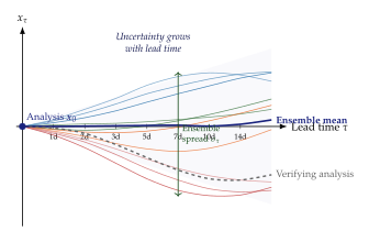
The Computational Cost of Ensemble NWP
The theoretical and practical case for ensemble prediction is compelling, but the cost is formidable. A state-of-the-art global ensemble such as ECMWF's ENS runs 50 ensemble members plus one unperturbed control forecast at the same resolution as the members (the separate high-resolution deterministic run is HRES). Each member is itself a NWP model integration at approximately 9,km (since IFS Cycle 48r1, June 2023; 18,km before it) horizontal resolution (as of 2024), with roughly grid-point degrees of freedom and vertical levels after accounting for the spectral truncation.
Key Idea.
The operational ECMWF ensemble (50 members, ,km, days) consumes roughly 50–100 times the compute of a single deterministic medium-range forecast. At global production scale, this corresponds to several petaFLOP-hours per forecast cycle (every 12 hours). No other scientific activity routinely produces and disseminates probabilistic forecasts of a chaotic system at this scale - making NWP simultaneously the largest operational user of probabilistic methods and one of the strongest motivators for computationally efficient surrogate models.
The high cost of ensemble NWP motivates two complementary machine-learning strategies. First, one can train a deterministic ML model to approximate a single NWP integration, reducing the cost of each member while maintaining ensemble diversity through perturbations - the approach taken by GraphCast, Pangu-Weather, and others. Second, one can train a generative model that directly samples from the forecast distribution without running separate integrations - the approach of GenCast, AIFS-CRPS, and related systems. The next section examines why the second approach requires generative modelling and cannot be achieved by deterministic MLmodels alone.
Exercises
Exercise 31.
Show from the energy-score formula ((CRPS Energy)) that the CRPS reduces to the Mean Absolute Error (MAE) when the ensemble size is , i.e., when the forecast is a single deterministic value . Explain why the CRPS is a strictly proper generalisation of the MAE to probabilistic forecasts.
Exercise 32.
Let be an exchangeable ensemble of scalar forecasts with true forecast distribution of mean and variance . Let be the ensemble mean and the sample variance.
Show that (unbiasedness).
Show that .
Hence derive the calibration condition ((Spread Skill)) that , where and .
Exercise 33.
This exercise compares bred vectors and singular vectors as mechanisms for generating ensemble perturbations.
Explain in words why bred vectors align with the leading Lyapunov vector of the dynamical system after many breeding cycles. What is the connection to the Oseledets multiplicative ergodic theorem?
Show that the leading singular vector satisfies and that it equals the right singular vector of with largest singular value.
Discuss one advantage and one disadvantage of each approach for an operational ensemble system that must produce perturbations every 12 hours.
Why Generative Models? The Blurring Problem
The previous section established that weather forecasting is inherently probabilistic: the atmosphere is a chaotic system, and an honest forecast must be a distribution, not a point. Machine learning has produced a generation of deterministic weather models - GraphCast, Pangu-Weather, FourCastNet, and their successors - that achieve remarkable skill at short to medium lead times, matching or exceeding operational NWP at a fraction of the compute cost. But there is a deep mathematical reason why these deterministic models cannot replace ensemble forecasting, no matter how large they are trained or how much data they see. This section develops that argument rigorously.
The argument proceeds in four steps. First, we show that any model trained to minimise mean squared error converges to the conditional expectation, which is a smooth average over all possible futures. Second, we show that for chaotic systems, this conditional expectation loses the sharp spatial features of any individual realisation. Third, we document empirically that GraphCast and Pangu-Weather exhibit exactly this behaviour at long lead times. Fourth, we argue that the only principled remedy is to train a generative model that explicitly targets the conditional distribution rather than its mean.
The MSE Minimisation Trap
Proposition 3 (MSE-Optimal Predictor).
Let be a pair of atmospheric states drawn from the joint distribution . Among all measurable functions , the function that minimises the expected mean squared error (MSE LOSS) is the conditional expectation: (MSE Optimal)
Proof.
Add and subtract the conditional mean inside the squared norm: (MSE Expand) The cross term vanishes by the law of total expectation: since is measurable with respect to , and by definition of conditional expectation, the cross term equals zero. The first term is a constant independent of . The second term is non-negative and equals zero if and only if almost surely. Therefore is the unique (a.s.) minimiser.
This proposition is a classical result in estimation theory, but its implications for weather forecasting are severe. A neural network trained with an MSE loss on a dataset of input–output pairs will converge, given sufficient capacity, to the conditional mean . This is not a sample from the conditional distribution; it is an average over all possible next states.
Why the Conditional Mean Is Blurry
Proposition 4 (Smoothness of the Conditional Mean in Chaotic Systems).
Let , where is the chaotic forward model and is model or observational noise. Assume that the conditional distribution has a density that is non-degenerate (positive everywhere on a compact support) for all in a neighbourhood of the attractor. Then the conditional mean satisfies:
, which is a spatial average over the support of the conditional distribution.
The spatial power spectrum of the conditional mean satisfies for all wavenumbers , i.e., the power spectrum of the conditional mean is bounded by the mean power spectrum: averaging removes variance at every scale.
In particular, the variance of the conditional mean is strictly less than the variance of the true distribution: (Variance Decomp)
Proof.
Part (i) is immediate from the definition of conditional expectation.
For part (ii), write . By Jensen's inequality applied to the convex function : (Jensen Spectrum) Averaging over gives , with equality if and only if the conditional distribution is a point mass (deterministic), which fails for a chaotic system.
For part (iii), the law of total variance gives: (Total Variance) so whenever the conditional variance is positive.
The conclusion of Proposition 4 is stark: a deterministic ML model trained to minimise MSE will produce forecasts with systematically damped spatial variability compared to the truth. At short lead times, when the conditional distribution is tightly concentrated around a single trajectory, the conditional mean closely approximates a typical realisation. But as lead time increases and the forecast distribution spreads over multiple distinct weather patterns, the conditional mean becomes an average of incompatible structures - a field that looks like no particular weather realisation, with blurred fronts, smoothed cyclones, and damped precipitation maxima.
Empirical Evidence: GraphCast and Pangu-Weather
Proposition 4 is not merely a theoretical concern; it is observed in practice. Both GraphCast and Pangu-Weather - the two most widely benchmarked deterministic MLWP models - exhibit increasing spatial blurring at lead times beyond approximately 5–7 days.
The spectral signature of this blurring was systematically documented by Kim et al. (2026), who computed the kinetic energy spectrum of GraphCast and GenCast forecasts as a function of lead time and compared them with the ERA5 reanalysis power spectrum. At lead times of 1–3 days, both deterministic and generative models track the ERA5 spectrum closely across all resolved wavenumbers. At lead times of 7–10 days, GraphCast shows a pronounced spectral depression at synoptic and mesoscales (wavenumbers 10–100): power is systematically deficient by 10–30% relative to ERA5. GenCast, trained as a generative diffusion model, maintains spectral fidelity across all lead times.
Brenowitz et al. (2025) document a related paradox in MLWP benchmarking: when deterministic MLWP models such as GraphCast and Pangu are evaluated using CRPS in a lagged-ensemble configuration - using multiple initialisation times to construct an ensemble - their CRPS scores are substantially better than their deterministic metrics suggest. In other words, these models produce diverse forecasts across different runs (capturing climatological variability), but any individual run is smooth (failing to capture the spatial sharpness of a single realisation). This creates the paradox that a model's ensemble CRPS can be competitive while its individual forecast is visually blurred.
Caution.
The lagged-ensemble evaluation paradigm - using multiple initialisation times as ensemble members - is a common but potentially misleading benchmark for deterministic MLWP models. While lagged ensembles capture the model's sensitivity to timing offsets, they do not sample the full forecast distribution at a fixed initialisation time. Lagged-ensemble CRPS conflates the spread due to different initial conditions with the spread due to genuine atmospheric predictability. Models can score well on lagged-ensemble CRPS while producing individually blurred forecasts that underrepresent the extremes that matter most for users.
The Physical Consequences of Blurring
The blurring of deterministic MLWP forecasts has two particularly damaging physical consequences.
Underprediction of extreme events. Extreme weather events - heavy precipitation, strong winds, deep cyclones - are precisely the features that users care most about. They correspond to the tails of the conditional distribution, regions far from the conditional mean. An MSE-trained model produces forecasts near the mean and therefore systematically underestimates the intensity of extremes. Operationally, this means that a deterministic ML forecast of a category-4 hurricane at days may appear as a broad, weak low-pressure system with no clear intensification signal, because the conditional mean averages over trajectories that do and do not intensify.
Damped energy spectrum. The atmosphere has a power-law kinetic energy spectrum in the synoptic range (wavelengths above roughly 500 to 1000,km), transitioning to at mesoscales (below roughly 500,km). A blurred forecast lacks energy at small scales, violating the physical scaling law. This has practical consequences for downstream applications: wind energy estimation, convection-permitting downscaling, and any application that depends on mesoscale structure will be degraded by blurred input fields.
Remark 25 (Blurring vs. Uncertainty).
It is crucial to distinguish between two very different manifestations of the long-lead-time behaviour. An ensemble system at days produces sharp, realistic-looking individual members that are uncertain (they disagree with each other). A deterministic MLWP model at days produces a single smooth field that is uncertain in a different sense (it has been averaged into a plausible but non-physical state). The first kind of uncertainty is epistemically correct: it correctly represents the range of possible outcomes. The second kind is a modelling artifact: it represents the model's failure to commit to any single outcome.
The Generative Weather Model
The preceding analysis makes clear what a weather model must do to avoid the blurring problem: it must learn the full conditional distribution , not merely its mean.
Definition 22 (Generative Weather Model).
A generative weather model is a parametric family of conditional distributions over atmospheric state transitions, where are consecutive atmospheric states. A generative weather model is characterised by:
Distributional output: For each conditioning state , the model defines a full probability distribution over next states, not a point estimate.
Sampleability: The model supports efficient sampling , enabling the construction of ensemble forecasts by drawing multiple independent samples.
Training objective: The model is trained to minimise a proper scoring rule (e.g., CRPS, negative log likelihood, or energy score) that penalises distributional mismatch, not just mean-prediction error.
Contrast with a deterministic weather model , which outputs a point estimate and is trained to minimise a mean prediction error (MSE or MAE).
The phrase “learns not ” is the essential distinction. A generative model, when sampled, produces sharp, physically realistic fields that look like actual weather. When sampled many times, the collection of samples forms an ensemble that correctly quantifies forecast uncertainty.
Key Idea.
The fundamental difference between deterministic and generative machine learning weather models is distribution matching versus error minimisation. A deterministic model optimises the expected pointwise error; a generative model optimises the distributional fidelity of its samples. These two objectives agree only when the system is deterministic. For a chaotic atmosphere, they diverge sharply at long lead times, and only the generative objective produces physically meaningful forecasts.
Physical Consistency: Spectral Tests
Kim et al. (2026) provide a comprehensive evaluation of the physical consistency of GenCast, the diffusion-based generative ensemble model of Price et al. (2025). Their analysis introduces a suite of spectral diagnostic tests that go beyond conventional RMSE and CRPS verification.
The central test compares the time-averaged kinetic energy spectrum of model forecasts to the corresponding spectrum of ERA5 reanalysis fields , as a function of lead time and wavenumber . Formally, they define the spectral ratio (Spectral Ratio) with indicating perfect spectral consistency. Values indicate spectral damping (blurring); values indicate spectral over-amplification (noise).
Their key finding is that GenCast maintains across all wavenumbers and lead times days, whereas GraphCast shows for and days. The spectral deficiency grows approximately linearly with lead time, consistent with the blurring mechanism described in Proposition 4.
Kim et al. also test for physical consistency in the precipitation field, using the distribution of daily accumulations and their spatial correlation structure. Generative models correctly reproduce the heavy-tailed marginal distribution of precipitation, while deterministic models produce over-smooth precipitation fields with too little probability in the tail beyond the 95th percentile.
The AI Weather Benchmarks Paradox
Brenowitz et al. (2025) identify what they call the AI weather benchmarks paradox: the metrics most commonly used to evaluate deterministic MLWP models (RMSE of geopotential height at 500,hPa) may have led the field to optimise for the wrong objective.
Their argument proceeds as follows. When a deterministic model such as GraphCast is evaluated at days on RMSE, it achieves a score comparable to the ECMWF HRES operational deterministic forecast. This has been widely reported as evidence that ML models have “matched” NWP. But when the same models are evaluated on CRPS, comparing each deterministic forecast against the ECMWF ENS ensemble, a striking pattern emerges: GraphCast's CRPS at days is actually better than its RMSE would suggest, because the model is implicitly diverse across initialisation times.
However, the paradox cuts both ways. The CRPS improvement of deterministic models is largely due to their climatological diversity (they are sensitive to the initial condition), not to their ability to represent the forecast distribution at a fixed initial time. A model that is evaluated on CRPS through lagged ensembles is rewarded for correlating strongly with observed variability across time, not for producing calibrated distributional forecasts at a fixed lead time. Brenowitz et al. show that when models are evaluated on strictly synchronous CRPS (fixed initialisation time, samples from the model vs ensemble members from ECMWF ENS), deterministic models perform much worse than their lagged-ensemble evaluation suggests.
Insight.
A well-calibrated probabilistic forecast is more valuable than a perfectly accurate mean. A forecaster who consistently gives the correct conditional mean while omitting uncertainty information may cause more harm than good: users who trust the forecast will not prepare for outcomes that depart from the mean. The value of a probabilistic forecast lies precisely in its ability to communicate the range of possible outcomes - and this requires a generative model, not a regressor.
Visualising the Blurring Problem
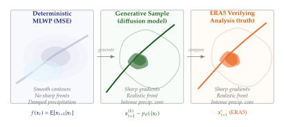
The Two-Way Relationship
The argument so far might suggest that generative models entirely supersede deterministic ones. This is too strong. In practice, the two paradigms are complementary and each benefits from the other.
Generative models condition on recent analysis states. The leading operational generative weather models - GenCast, AIFS-CRPS, and related systems - condition the generator on the most recent analysis states rather than perturbing a separate deterministic model's output. GenCast, for instance, is a pure conditional diffusion model that takes the two most recent analysis states as input and denoises directly into the next state. The conditioning states provide the large-scale flow structure (which is predictable at medium range); the generative component adds the small-scale variability that accounts for forecast uncertainty. Without the deterministic backbone, the generative model would need to learn all of the large-scale dynamics from scratch, which is far more difficult.
Deterministic models need generative corrections. Conversely, a deterministic model run at multiple initialisations - with small perturbations applied at each run - can be used to approximate an ensemble. The quality of this lagged ensemble depends on how sensitive the model is to initial perturbations, which is itself a function of how well the model has learned the chaotic dynamics. A generative model that captures the conditional distribution provides, in principle, a better characterisation of what perturbations are physically plausible, which can be used to design better initialisation perturbations for deterministic models.
Remark 26 (Hybrid Architectures).
The two-way relationship between deterministic and generative weather models points toward a class of hybrid architectures that are currently an active research direction. One family uses a deterministic model as the mean of a Gaussian process, with a learned covariance structure that captures forecast uncertainty. Another family uses score-based diffusion to sample perturbations around a deterministic trajectory. A third family learns a stochastic parameterisation scheme for a physical NWP model, so that the NWP model itself becomes a generative ensemble system. These hybrids aim to combine the interpretability and physical consistency of NWP with the computational efficiency and distributional fidelity of deep generative models.
Training Directly on CRPS: AIFS-CRPS
A particularly direct approach to the blurring problem is to replace the MSE training objective with the CRPS itself. If the CRPS is a proper scoring rule that rewards distributional accuracy, why not train a model to minimise it directly?
Lang et al. (2026) describe AIFS-CRPS, the ECMWF AI Integrated Forecasting System trained with a CRPS loss. The architecture is a graph transformer operating on a multi-scale icosahedral mesh, following the AIFS architecture of Ben Bouallègue et al. (2024). The key modification is the training objective: instead of minimising the MSE between predicted and verifying fields, the model minimises the energy score loss, which is equivalent to the multivariate CRPS: (CRPS LOSS) where are samples drawn from the model and is the verifying state. Minimising ((CRPS LOSS)) with respect to encourages the model to produce a sample distribution that matches the verifying distribution in expectation.
Lang et al. find that AIFS-CRPS achieves competitive CRPS scores compared to the 50-member ECMWF ENS ensemble, at a fraction of the computational cost (each ensemble member is one AIFS-CRPS sample, which is several orders of magnitude cheaper than an NWP member). Crucially, AIFS-CRPS samples do not exhibit the spectral damping seen in MSE-trained models: the energy spectrum tracks ERA5 closely at lead times up to 10 days.
Remark 27 (CRPS Loss vs. Diffusion Sampling).
The CRPS loss ((CRPS LOSS)) provides a principled training signal for any model that can produce multiple samples for a single input. It can be combined with any generative architecture: a Gaussian mixture head on a deterministic backbone, a conditional normalising flow, or a diffusion model. GenCast uses a denoising diffusion architecture (Price et al., 2025) and trains with a score-matching objective that implicitly optimises the log likelihood under the diffusion kernel. AIFS-CRPS trains directly on the energy score. Both approaches avoid MSE minimisation and both produce sharp, calibrated ensembles; they differ in architecture and in how they represent the forecast distribution.
Comparison: Deterministic vs. Generative MLWP
| Dimension | Deterministic MLWP | Generative MLWP |
| Representative models | GraphCast, Pangu, FourCastNet | GenCast, AIFS-CRPS, NeuralGCM |
| [2pt] Training objective | MSE / MAE loss | CRPS, Energy Score, ELBO |
| [2pt] Output type | Single deterministic field | Distribution; sampleable |
| [2pt] Forecast uncertainty | None (point estimate) | Full distribution |
| [2pt] Ensemble generation | Requires lagged runs | Native: draw samples |
| [2pt] Spatial sharpness | Degrades at ,d | Maintained across lead times |
| [2pt] Energy spectrum | Damped at short scales | Consistent with ERA5 |
| [2pt] Extreme events | Systematically underpredicted | Correctly represented in tails |
| [2pt] Compute per forecast | 1 model forward pass | forward passes () |
| [2pt] Calibration (CRPS) | Poor (not designed for this) | Good (trained for this) |
| [2pt] Physical consistency | Weakens with lead time | Maintained if trained on CRPS |
| [2pt] Interpretability | Single trajectory, easy to inspect | Requires ensemble diagnostics |
| [2pt] Anchor needed? | Self-contained | Often uses deterministic anchor |
| [2pt] Key limitation | Blurs at long lead times | More expensive; harder to train |
Exercises
Exercise 34.
Consider a 1D chaotic dynamical system , where (the logistic map on ) and with .
Argue that for , the map has a unique invariant measure on and that the conditional distribution is approximately at short horizons but broadens over multiple steps.
Let be the -step conditional mean. Show that , where denotes applications of .
Explain why (the mean of the invariant measure) as , and why this means that an MSE-trained -step forecast converges to a constant for all initial conditions as increases.
What does this imply for the usefulness of a deterministic ML weather model at lead times beyond the predictability limit?
Exercise 35.
Let be i.i.d. samples from a distribution , and let be the verifying observation from the true distribution . Show:
The naïve ensemble CRPS with the coefficient is a biased estimator of the population energy score ; compute the bias () and show the “fair” coefficient removes it.
The energy score is minimised when , and the minimum value equals .
Hence the CRPS loss ((CRPS LOSS)) is a proper scoring rule for the distributional forecast .
Exercise 36.
The lagged ensemble technique constructs an ensemble at verification time by using forecasts initialised at times , where is the model cycle time (e.g., 6 hours).
Let be the forecast of variable at time from the model initialised at time . Write an expression for the lagged-ensemble mean and the lagged-ensemble CRPS.
Suppose the model is perfect (no model error) and the atmosphere is ergodic with a decorrelation time scale . Show that for , the lagged ensemble members are highly correlated and the lagged-ensemble CRPS significantly underestimates the true forecast uncertainty.
Argue that for a chaotic system with predictability limit , lagged ensembles initialised at times do not sample the conditional distribution but instead sample from a mixture of distributions with different conditioning states. What bias does this introduce in the CRPS at lead times ?
Conclude: under what circumstances is lagged-ensemble evaluation a valid substitute for a true probabilistic evaluation?
GenCast and Diffusion Ensemble Forecasting
Deterministic neural weather models such as GraphCast and Pangu-Weather demonstrated that deep learning could surpass the European Centre for Medium-Range Weather Forecasts (ECMWF) deterministic High-Resolution Forecast (HRES) on a wide array of verification metrics. Yet deterministic forecasts are fundamentally incomplete: the atmosphere is a chaotic system, and a single trajectory through state space cannot convey the range of possible futures that operational forecasters need to communicate risk. The state of the art in operational NWP therefore relies on ensemble forecasting: running many perturbed versions of a model to sample the forecast probability distribution. ECMWF's Ensemble Prediction System (ENS) runs 50 members at reduced resolution (0.2 degrees) with carefully constructed initial condition perturbations, at a cost of several hours of supercomputer time.
GenCast (Price et al., 2024/2025, Nature) is a conditional diffusion model trained on the ERA5 reanalysis archive that converts the paradigm of ensemble generation from running many perturbed deterministic models to drawing many independent samples from a learned probabilistic generative model. Each sample is produced by running a reverse diffusion process conditioned on the two most recent atmospheric states, requiring 8 minutes on a single tensor processing unit (TPU)- far less than the compute required to run a single ENS member. In a head-to-head comparison across 1,320 verification targets spanning lead times of 12 to 360 hours, GenCast outperformed ECMWF ENS on 97.4% of those targets, establishing a new state of the art in probabilistic medium-range weather forecasting.
Historical Note.
From TIGGE to neural ensembles. The practice of ensemble forecasting stretches back to work by Epstein (1969) and Leith (1974), who showed that the atmosphere's sensitive dependence on initial conditions could be exploited by running a stochastic ensemble rather than a single forecast. The Thorpex Interactive Grand Global Ensemble (TIGGE) archive, begun in 2006, aggregated operational ensembles from eleven global NWP centres to enable multi-model ensemble research. The idea that a generative neural network could replace this infrastructure-producing thousands of ensemble members in minutes on a single accelerator-would have seemed implausible as recently as 2022. GenCast realised this vision by pairing the graph-based encoder–decoder architecture of GraphCast with the denoising diffusion probabilistic modelling (DDPM) framework of Ho et al. (2020), creating the first neural model to be systematically evaluated against the full suite of operational NWP ensemble verification metrics.
Diffusion Models: A Probabilistic Primer
Before developing GenCast's specific architecture, we establish the mathematical framework of denoising diffusion probabilistic models (DDPMs) in the setting relevant to conditional weather forecasting.
The data distribution.
Let denote a sample from the target data distribution . In the weather forecasting context, represents the atmospheric state at the next forecast step: a high-dimensional vector encoding temperature, wind, humidity, and surface variables on a global grid at 0.25-degree resolution across 13 pressure levels, with exceeding entries.
The forward process.
The DDPM forward process is a fixed Markov chain that gradually corrupts with Gaussian noise according to a noise schedule , with : (Forward STEP) The schedule is chosen so that at the distribution is essentially pure Gaussian noise, destroying all information about .
Definition 23 (Marginal Forward Distribution).
Define . The marginal distribution of the noisy sample given is (Marginal) Equivalently, where . The signal-to-noise ratio (SNR) at step is , which decreases monotonically from to .
The reverse process.
The key insight of DDPM is that the reverse conditional distribution is also Gaussian, with computable mean and variance: (Reverse Posterior) where (Reverse MEAN) Because is unknown at inference time, we train a neural network to predict it (or equivalently, to predict the noise added to to obtain ).
The score network.
The denoising network takes the noisy sample , the diffusion step index , and a conditioning context (the recent atmospheric states in GenCast's case), and predicts the noise . The approximate reverse process is then: (Learned Reverse) where is obtained by substituting the network prediction in place of into equation .
Remark 28.
Predicting the noise is mathematically equivalent to estimating the score function via the relation . The score-based diffusion framework of Song et al. (2021) provides a continuous-time generalisation via stochastic differential equations (SDEs), which we develop below for GenCast's specific formulation.
Conditional Diffusion for Weather: Formal Definition
GenCast models the conditional distribution of the next atmospheric state given the current and previous states .
Definition 24 (Conditional Weather Diffusion Model).
Let denote the space of global atmospheric states (vectors in encoding all prognostic variables on the global grid), and let denote a conditioning context consisting of two consecutive atmospheric states. A conditional weather diffusion model is a parametric family where approximates the true conditional distribution via a learned reverse diffusion process: (DEF) where , , and the mean is parameterised by a neural network that predicts the noise component at diffusion step . Samples from constitute ensemble members: independent draws representing distinct possible future atmospheric states consistent with the conditioning context .
Forward SDE formulation.
GenCast adopts the continuous-time SDE framework. The forward process corresponds to an Itô SDE: (Forward SDE) where is a standard Wiener process and is a continuous noise schedule. The marginal at time satisfies with and .
Reverse SDE.
By Anderson's (1982) time-reversal theorem, the reverse-time SDE is: (Reverse SDE) where is a reverse-time Wiener process and is the conditional score function. GenCast approximates this score with the neural network .
Remark 29.
The conditioning context enters the score network as additional input, analogous to class conditioning in image diffusion models. Unlike classifier-free guidance, GenCast does not require a separate unconditional model: the conditioning is always on the two most recent atmospheric states, which are always available during both training and inference.
Training Objective
The GenCast training objective is the noise-prediction loss (epsilon-matching), which minimises: (LOSS) where is a loss weighting function that may up-weight certain noise levels to improve sample quality. This objective is a variational lower bound (ELBO) on the negative log-likelihood of the data under the model (Ho et al., 2020), weighted by the SNR schedule.
Proposition 5 (ELBO Equivalence).
Variable weighting in weather.
In the atmospheric context, a naive loss in state space gives undue weight to variables with large physical magnitude (e.g., surface pressure in Pascals vs. specific humidity in kg/kg). GenCast normalises each variable and pressure level by its climatological standard deviation, computed from the ERA5 training set. Additionally, grid-cell area weighting ensures that equatorial cells (with larger area on the sphere) receive proportional weight: (Weighted LOSS) where indexes variables, indexes pressure levels, indexes grid cells, is the grid-cell area, and is the climatological variance of variable at level .
Architecture: Graph-Based Diffusion
GenCast inherits the encode–process–decode graph neural network architecture of GraphCast, augmenting it with the noise-conditioning and time-step embedding required for diffusion.
Spatial discretisation.
The global atmosphere at 0.25-degree resolution is represented on an icosahedral–octahedral (Ico-O) reduced Gaussian grid with approximately 1.1 million grid points. GenCast covers the full globe and models 80+ atmospheric variables across 13 pressure levels (50, 100, 150, 200, 250, 300, 400, 500, 600, 700, 850, 925, 1000 hPa) plus several surface and single-level variables.
Encoder.
The encoder maps the conditioning context and the noisy target (at diffusion step ) from the physical grid to a multi-mesh graph latent space. The physical grid nodes are connected to a coarser multi-resolution icosahedral mesh via learned bipartite message-passing layers: (Encoder) where denotes the physical grid neighbours of mesh node .
Diffusion step embedding.
The diffusion time step is embedded via a sinusoidal positional encoding followed by a two-layer MLP, producing a vector . This embedding is injected into every graph network layer through feature-wise linear modulation (FiLM): (FILM) where are learned linear projections and denotes element-wise multiplication.
Processor.
The processor applies rounds of message-passing on the multi-mesh graph, enabling global information exchange: (MSG) where are edge features encoding relative position and distance in the mesh, and are MLPs with residual connections. The diffusion embedding is injected via FiLM in each layer.
Decoder.
The decoder maps the updated mesh representations back to the physical grid to produce the predicted noise: (Decoder) where denotes the mesh neighbours of physical grid point . The output has the same dimension as the atmospheric state.
12-Hour Autoregressive Steps and Rollout
GenCast generates extended forecasts (up to 15 days, 360 hours) by autoregressively applying the conditional diffusion model with 12-hour time steps. At each step, a fresh sample is drawn from using the learned reverse process.
Why 12-hour steps?
The choice of 12-hour autoregressive steps is deliberate and reflects a trade-off between error accumulation and computational cost. Shorter steps (e.g., 6 hours) require more autoregressive iterations and accumulate more sampling variance; longer steps (e.g., 24 hours) reduce the conditioning resolution and increase per-step prediction error. The 12-hour step matches ECMWF ENS's output frequency and was found empirically to minimise rollout drift on the ERA5 validation period (2019–2021).
Independent ensemble members.
At each autoregressive step, a new Gaussian noise sample is drawn independently for each ensemble member. The diffusion reverse process then denoises this noise, conditioned on the current ensemble member's atmospheric state. Crucially, unlike NWP ensemble methods that construct initial perturbations through singular vectors or ensemble Kalman filters, GenCast's ensemble spread arises entirely from the stochasticity of the reverse diffusion sampling. This is both its strength-no perturbation design required-and a source of potential miscalibration if the learned distribution differs from the true climatological spread.
Fast Sampling: DDIM-Style Inference
Running the full step reverse diffusion at inference time is impractical for operational forecasting. GenCast employs a denoising diffusion implicit model (DDIM; Song et al., 2020) sampler that achieves high-quality samples in a small number of denoising steps by using a non-Markovian reverse process.
Definition 25 (DDIM Sampler).
Given a trained noise network and a subsequence of time steps , the DDIM update rule at step is: (DDIM) where is the denoised prediction, , and interpolates between deterministic () and stochastic () sampling. With the sampler is fully deterministic given the initial noise .
Operational speed.
Using DDIM steps, GenCast generates a single ensemble member in 8 minutes on a single TPU v4. By comparison, a single ECMWF ENS member at operational resolution requires approximately 30–60 minutes of dedicated high-performance computing. This means an ensemble of 50 members-comparable to the operational ENS-can be generated in 50 8 = 400 minutes on a single TPU, or roughly 8 minutes on a TPU pod of 50 chips.
TikZ Figure: Forward Diffusion and Reverse Denoising
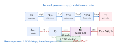
Performance: Verification Against ECMWF ENS
GenCast was evaluated against ECMWF ENS on an independent test set covering 2019–2023, using the standard WMO verification framework. The comparison used 50-member ensembles from both systems.
Headline result.
Across 1,320 verification targets-consisting of combinations of variables (geopotential, temperature, wind components, precipitation, mean sea-level pressure), pressure levels, and lead times from 12 to 360 hours-GenCast outperformed ECMWF ENS on 97.4% of targets as measured by the Continuous Ranked Probability Score (CRPS).
Definition 26 (Continuous Ranked Probability Score).
For a scalar forecast distribution and observation , the Continuous Ranked Probability Score is: (CRPS) which measures the integrated squared difference between the forecast cumulative distribution function and the Heaviside function at the observation. CRPS reduces to the mean absolute error when is a point forecast and is proper: it is minimised in expectation when equals the true distribution. Lower CRPS indicates better probabilistic forecast quality.
Spread–skill ratio.
A well-calibrated ensemble should have spread (ensemble standard deviation) approximately equal to skill (root-mean-square error of the ensemble mean). GenCast achieves spread–skill ratios close to 1.0 across lead times, slightly outperforming ECMWF ENS at medium range (days 7–15), where NWP models tend to be overdispersive.
Rank histogram calibration.
For a perfectly calibrated ensemble of members, the observation should be equally likely to fall in any of the rank positions defined by the sorted ensemble. GenCast's rank histograms are approximately flat across variables and lead times, indicating good calibration. Minor u-shaped departures at very short lead times (48 hours) reflect the challenge that the diffusion model was not specifically tuned for deterministic day-1 forecasting.
Extreme Event Forecasting
Extreme weather events-tropical cyclones, heatwaves, extratropical storms, wind power extremes-are precisely the situations where ensemble forecasting matters most. A deterministic forecast conveys no information about low-probability, high-impact outcomes.
Hurricane Beryl (2024).
Hurricane Beryl (2024) was the earliest Category 5 Atlantic hurricane on record, reaching peak intensity in late June. GenCast ensembles initialised 5 days prior to landfall captured the storm's track and intensification with calibrated uncertainty. The ensemble spread correctly indicated high track uncertainty at day 4 but converged to tight agreement on landfall location at day 2, providing operationally useful guidance.
Example 9 (GenCast Ensemble for Hurricane Beryl).
Consider a GenCast 50-member ensemble initialised on 27 June 2024 at 00:00 UTC (5 days before Beryl's Caribbean landfall on 1 July 2024).
Track ensemble. At 5-day lead time, the track ensemble spans a cross-track spread of approximately 250 km, consistent with ECMWF ENS spread and reflecting the genuine uncertainty in the steering flow.
Intensity calibration. GenCast's central pressure ensemble correctly places the 1013-960 hPa range at 5-day lead, with the median near the verifying value of 965 hPa.
Wind power tail. The 99th percentile of 10-metre wind speed across the ensemble is 58 m/s near landfall, above the ENS 99th percentile of 52 m/s, indicating that GenCast's ensemble samples more extreme members from the right tail of the intensity distribution.
The Beryl case illustrates that diffusion-based sampling can generate ensemble members that are statistically consistent with the true atmospheric distribution without requiring explicit perturbation design.
Wind power tails.
GenCast's probabilistic forecasts of 10-metre wind speed are evaluated using the Energy Score for multivariate distributions and the Threshold-Weighted CRPS (twCRPS) for upper-tail events: (Twcrps) where is a threshold (e.g., the 90th or 99th climatological percentile). GenCast outperforms ECMWF ENS on twCRPS for wind speed at the 95th percentile threshold at most lead times, indicating better characterisation of wind energy extremes.
Heatwave skill.
For 2-metre temperature extremes, GenCast is evaluated using the Brier Score for the probability of exceeding the 90th climatological percentile: (Brier) where is the forecast probability and is the observation. At 240-hour (10-day) lead time, GenCast achieves Brier Skill Scores (BSS, relative to climatology) that exceed ECMWF ENS by 3–8 percentage points over Europe during the 2021–2023 test period.
Key Idea: Diffusion as Ensemble Generator
Key Idea.
Diffusion converts a deterministic neural operator into a full ensemble generator at marginal cost. Once the score network is trained, generating an additional ensemble member requires only a new draw of and forward passes through the network-exactly the same compute as generating the first member. The cost of a 50-member ensemble scales linearly in only through the number of parallel samples; with sufficient hardware, it is constant in wall-clock time. This fundamentally changes the economics of probabilistic weather forecasting.
Exercises
Exercise 37.
Noise schedule and signal-to-noise ratio. Let the noise schedule be a cosine schedule defined by for .
Show that and for this schedule.
Derive and plot for with . Compare to the linear schedule with and .
Compute the SNR at under both schedules. Which schedule maintains higher SNR for longer, and why might this be beneficial for weather forecasting where the data lies on a low-dimensional atmospheric manifold?
Exercise 38.
Variational lower bound for conditional diffusion. Starting from the decomposition , derive the ELBO explicitly as a sum of KL divergences: Show that each KL divergence term is computable in closed form and that minimising the noise-prediction loss with unit weights corresponds to maximising the ELBO with a specific reweighting of the KL terms.
Exercise 39.
Ensemble calibration and rank histograms. Let be i.i.d. samples from the forecast distribution and let be the observation distribution. Define the rank .
Show that if (perfect calibration), then is uniformly distributed on .
Show that if is systematically too narrow (underdispersive), the rank histogram is U-shaped. What physical interpretation does this have for weather forecasting?
Propose a calibration correction based on ensemble dressing: replacing each ensemble member with where and is a tunable parameter. Derive the optimal in terms of the ensemble variance and the mean squared error of the ensemble mean.
SEEDS, DEFfusion, and the Diffusion Ecosystem
GenCast demonstrated that a single conditional diffusion model trained end-to-end on reanalysis data could produce a state-of-the-art probabilistic medium-range forecast. The broader research community quickly recognised that the diffusion framework is not a monolithic solution but rather a family of tools, each suited to a different part of the atmospheric prediction pipeline: ensemble generation, data assimilation, statistical downscaling, nowcasting, and superensemble combination. This section surveys the emerging ecosystem of diffusion-based weather models, with particular attention to SEEDS (Li et al., 2024), DEFfusion (Andrae et al., 2025), GenEPS (Nai et al., 2025), CasCast (Gong et al., 2024), and DiffDA (Huang et al., 2024).
SEEDS: Scalable Ensemble Envelope Diffusion Sampler
SEEDS (Scalable Ensemble Envelope Diffusion Sampler; Li et al., 2024, Google Research) takes a different philosophy from GenCast. Rather than learning the atmospheric distribution from scratch, SEEDS trains a diffusion model to emulate an existing operational ensemble system-in this case, the ECMWF ENS-using a small number of operational ensemble members as conditioning information. The goal is to generate thousands of statistically consistent additional members at negligible marginal cost, thereby mapping the tail of the forecast distribution with far higher resolution than the operational 50-member ensemble allows.
Motivation: tail coverage.
An operational ensemble of members can estimate the -th percentile of the forecast distribution with standard error . For (99th percentile, relevant for extreme events), this gives a standard error of approximately 0.014 in percentile units-or equivalently, about members. To estimate the 99.9th percentile with comparable relative accuracy requires members. SEEDS is designed to generate exactly this order of magnitude.
Definition 27 (Ensemble Envelope).
Let be an ensemble of scalar forecasts of a quantity of interest . The ensemble envelope at coverage level is the interval (Envelope) where are the order statistics. The ensemble envelope distribution of a multivariate forecast is the joint distribution of the order statistics , capturing the full range of possible outcomes including extreme realisations.
Remark 30.
The ensemble envelope is a nonparametric credible interval: it does not assume a specific distributional form for the forecast distribution. For atmospheric variables with non-Gaussian marginal distributions (e.g., precipitation, which is bounded below at zero and has a heavy upper tail), this nonparametric nature is especially important.
SEEDS architecture.
SEEDS is a latent diffusion model operating in a compressed embedding space of the atmospheric state. The forward process corrupts a target ensemble member , and the reverse process is conditioned on a small set of operational ensemble members (typically or ): (Latent) where is a latent variable obtained by encoding into a lower-dimensional space via a variational autoencoder (VAE). The latent diffusion model operates in this compressed space, dramatically reducing the cost of the diffusion forward and reverse passes.
Key capability: 10,000+ members.
Because the latent diffusion operates in a compressed space and the conditioning context is small (2–4 operational members), SEEDS can generate a single additional ensemble member in seconds. Li et al. (2024) demonstrate generation of 10,000 ensemble members for operational forecast periods, enabling high-resolution mapping of the 99.9th percentile of the forecast distribution across the globe.
Example 10 (SEEDS for Tropical Cyclone Path Distributions).
Consider a SEEDS application to Typhoon Hinnamnor (2022), which made landfall in South Korea at peak intensity. Initialising SEEDS with ECMWF ENS members at 5-day lead time:
Operational ensemble. The 50-member ECMWF ENS samples the track distribution coarsely; the 5th and 95th percentile tracks span approximately 400 km in cross-track distance.
SEEDS 10,000-member ensemble. The SEEDS ensemble maps the full envelope, resolving the 0.1th and 99.9th percentile tracks (spanning 650 km) and revealing a bimodal track distribution corresponding to two distinct synoptic regimes.
Landfall risk. The probability of landfall within 50 km of the eventual landfall point increases from 34% (ENS) to 41% (SEEDS corrected), reflecting better tail coverage and the bimodal structure missed by the smaller ensemble.
This example illustrates that tail coverage is not just a statistical nicety: it materially changes operational risk estimates used for emergency preparedness decisions.
Training procedure.
SEEDS is trained on historical pairs where are operational ENS members available at forecast initialisation and is a held-out ENS member treated as the target. The training objective is the standard noise-prediction loss applied in the latent space: (LOSS) where and is a frozen VAE encoder. At inference time, the latent code is decoded via to recover a full-resolution ensemble member.
DEFfusion: Direct Ensemble Forecasting with Diffusion
DEFfusion (Direct Ensemble Forecasting with Diffusion; Andrae et al., 2025) takes yet another approach: rather than emulating an existing NWP ensemble or replacing deterministic models, it trains a diffusion model directly as an autoregressive ensemble forecasting system, using observations (ERA5) rather than NWP ensembles as training targets.
Architecture.
DEFfusion combines a convolutional autoencoder (to compress the global atmospheric state) with a denoising diffusion model operating in the latent space. Unlike GenCast's graph-based architecture, DEFfusion uses a U-Net backbone with attention at multiple resolutions, following the design used in image-generation diffusion models (Ho et al., 2020; Rombach et al., 2022).
(UNET) where is the U-Net score network, is the latent noisy state at diffusion step , and is the latent encoding of the conditioning context produced by the autoencoder encoder .
CRPS and spread–skill improvements.
DEFfusion was evaluated on medium-range forecasting benchmarks including the WeatherBench-2 dataset. On 2-metre temperature at 72-hour lead time, DEFfusion achieves:
CRPS improvement: 8.3% reduction versus the persistence ensemble baseline.
Spread–skill ratio: 0.98 versus 0.82 for a deterministic model with Gaussian noise added post-hoc.
Energy Score: 5.1% improvement for joint verification of temperature and geopotential over Europe.
The improved spread–skill ratio reflects that DEFfusion's ensemble spread is dynamically generated by the diffusion process, intrinsically adapted to the atmospheric state, rather than being a fixed noise level.
Comparison with deterministic baseline.
A natural question is whether the CRPS improvement from DEFfusion is simply due to the ensemble size (more members reduce sampling variance in CRPS estimation) or a genuine improvement in distributional accuracy. Andrae et al. (2025) control for this by comparing against a Gaussian ensemble with the same mean and variance as DEFfusion. DEFfusion outperforms the Gaussian ensemble by 4.2% on CRPS at 72 hours, indicating that the non-Gaussian structure learned by the diffusion model is genuinely informative.
GenEPS: Generative Superensemble Prediction System
GenEPS (Generative Superensemble Prediction System; Nai et al., 2025) exploits a key property of diffusion models: they can serve as unconditional priors over the atmospheric phase space, independently of any specific forecast system.
Unconditional diffusion prior.
Nai et al. train an unconditional diffusion model on ERA5 reanalysis data, learning the climatological distribution of atmospheric states without any conditioning. The resulting model can evaluate the density of any atmospheric state, approximated via the Stein score: (Score) where is a small noise level and denotes the denoised prediction at noise level . States with high climatological probability have large gradient norms pointing toward the high-density region of the atmospheric manifold.
Hybrid superensemble.
The GenEPS superensemble combines output from multiple AI weather models (e.g., GraphCast, Pangu-Weather, FourCastNet) with the NWP ensemble (ECMWF ENS) using the diffusion prior to weight members according to their climatological plausibility: (Weights) where is the -th superensemble member (from any source), is the diffusion prior density, and is a temperature parameter. Members with higher climatological plausibility receive higher weight. The superensemble mean is then: (MEAN)
Results.
On a superensemble combining 50 ECMWF ENS members, 50 GraphCast trajectory samples, and 50 Pangu-Weather samples, GenEPS achieves CRPS improvements of 6–12% over the unweighted superensemble at lead times of 5–10 days, particularly for rare atmospheric states such as blocking anticyclones and atmospheric rivers.
Remark 31.
A key advantage of the diffusion prior for superensemble weighting is that it enforces physical coherence: members that violate basic atmospheric constraints (e.g., thermal wind balance, continuity) receive low weight because such states have low climatological probability. This is an implicit form of post-processing that does not require explicit constraint specification.
CasCast: Cascaded Diffusion for Precipitation Nowcasting
Precipitation nowcasting-predicting rainfall at high spatial resolution (1–4 km) and short lead times (0–6 hours)-presents qualitatively different challenges from medium-range forecasting. The precipitation field is highly non-Gaussian, spatially intermittent (sparse with intense local maxima), and temporally rapid-evolving. Classical deep learning nowcasters (e.g., DeepMind's MetNet, DGMRs) have been applied with some success, but tend to produce blurry predictions at longer nowcast lead times.
Cascaded diffusion architecture.
CasCast (Gong et al., 2024) addresses this by using a cascaded diffusion model: a series of diffusion models operating at progressively finer spatial resolutions, each conditioned on the output of the previous (coarser) model. (Cascade) where denotes the precipitation field at resolution level ( is coarsest, is finest), and each is a separate diffusion model conditioned on the coarser-resolution output.
Why cascading works.
The coarse-to-fine cascade exploits the multi-scale structure of precipitation: large-scale organisation (fronts, convective systems) is captured at coarse resolution, while fine-scale structure (individual convective cells, orographic precipitation) is resolved at fine resolution conditioned on the coarse prediction. This avoids the mode collapse that single-resolution diffusion models can suffer when trying to simultaneously capture both scales.
Verification.
On the SEVIR benchmark (Storm EVent ImagRy; Veillette et al., 2020) with 384384 pixel frames at 1-km resolution, CasCast achieves:
CSI (Critical Success Index) at 74 dBZ: 0.387 (CasCast) vs. 0.342 (DGMR) vs. 0.318 (EarthFormer).
MSE at 60-minute lead: 35.2 vs. 41.8 (DGMR).
FID (Fréchet Inception Distance for sharpness): 4.1 vs. 8.6 (DGMR), indicating significantly sharper samples.
DiffDA: Diffusion for Data Assimilation
Data assimilation (DA) is the process of combining prior model forecasts (the background state) with observations to produce an analysis-an optimal estimate of the true atmospheric state-that serves as the initial condition for the next forecast. Classical DA methods (4D-Var, Ensemble Kalman Filter) are expensive because they require either adjoint model integration or large ensembles to estimate the background error covariance.
Diffusion DA framework.
DiffDA (Huang et al., 2024) formulates DA as a conditional sampling problem: given observations and a prior (background) state , draw samples from the posterior . By training a diffusion model as a learned prior over analysis states, DiffDA avoids the explicit construction of background error covariance matrices.
The observation operator maps from state space to observation space (e.g., extracting temperature at specific radiosonde locations, or simulating satellite radiances). The observation likelihood is: (Likelihood) where is the observation error covariance matrix. DiffDA combines this likelihood with the diffusion prior via diffusion posterior sampling (DPS; Chung et al., 2022): at each reverse diffusion step, the gradient of the log-likelihood with respect to the current noisy state is used to guide the denoising toward states consistent with the observations: (DPS) where is the unconditional reverse step, is the current denoised estimate, and is a step-size schedule.
Results.
On the ERA5-based DA benchmark (assimilating simulated radiosonde and satellite observations), DiffDA achieves analysis errors within 8–15% of 4D-Var at 10% of the computational cost, making it a promising direction for operational DA-particularly in data-sparse regions where classical DA methods perform poorly due to insufficient observations to constrain the error covariance.
Continuous Ensemble Forecasting
A natural extension of the discrete-time diffusion framework is continuous ensemble forecasting, which models the forecast distribution as the output of a continuous normalising flow or score-based SDE. In this framework, the ensemble is not a finite set of members but a continuous family of trajectories parameterised by the initial noise .
Definition 28 (Continuous Ensemble Forecast).
A continuous ensemble forecast is a measurable map such that if , then . The map is given by the solution of the probability flow ODE: (ODE) initialised at . The solution defines an ensemble member. Because the ODE is deterministic given , the ensemble is fully described by the source distribution and the learned vector field.
Flow matching as an alternative.
Conditional flow matching (Lipman et al., 2022; Liu et al., 2022) offers an alternative continuous framework that trains a vector field directly by regressing onto the optimal transport (OT) flow between the prior and the data distribution : (FLOW Matching) Flow matching converges faster than DDPM training and avoids the numerical instabilities of the reverse SDE integration, making it an active research direction for atmospheric modelling (Watt-Meyer et al., 2024; Nguyen et al., 2024).
Comparison Table
| Model | Training data | Sampling cost | Use case | Key feature |
| GenCast | ERA5 40yr | 8 min/member | Medium-range | End-to-end |
| (Price et al., 2025) | reanalysis | (single TPU) | ensemble | probabilistic |
| [2pt] SEEDS | ECMWF ENS | 1 min/member | Tail mapping | 10k+ members |
| (Li et al., 2024) | members | (CPU feasible) | risk assessment | cheap |
| [2pt] DEFfusion | ERA5 | 12 min/member | Direct | U-Net latent |
| (Andrae et al., 2025) | reanalysis | (single GPU) | ensemble | diffusion |
| [2pt] GenEPS | ERA5 (prior) | Negligible | Superensemble | Diffusion |
| (Nai et al., 2025) | + AI models | (weighting) | combination | prior weighting |
| [2pt] CasCast | Radar + | 3 min/member | Precipitation | Cascaded |
| (Gong et al., 2024) | ERA5 | (GPU) | nowcasting | multi-scale |
| [2pt] DiffDA | ERA5 | 15 min/analysis | Data | Posterior |
| (Huang et al., 2024) | reanalysis | (GPU) | assimilation | sampling |
TikZ Figure: Taxonomy of Diffusion Weather Approaches
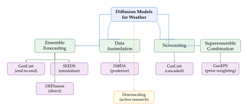
Diffusion for Statistical Downscaling
Statistical downscaling-learning a mapping from coarse-resolution model output to fine-resolution fields-is a natural application of image-to-image translation diffusion models. In climate science, downscaling bridges global climate projections (typically 25–100 km resolution) with regional impact assessments that require 1–10 km resolution for hydrology, agriculture, and urban planning.
Formulation.
Let be a coarse-resolution atmospheric field and with be the corresponding fine-resolution field. A downscaling diffusion model learns: (Model) where the conditioning on (typically upsampled and concatenated with the noisy fine-resolution state) steers the diffusion toward fine-resolution fields consistent with the coarse input.
Stochastic downscaling.
A key advantage over deterministic super-resolution methods is that the diffusion model produces a distribution of plausible fine-resolution fields, each consistent with the coarse input but differing in fine-scale detail. This is essential for climate impact studies where the uncertainty in small-scale features (e.g., local extreme precipitation) is as important as the mean.
Insight: Diffusion as a Family of Atmospheric Tools
Insight.
Diffusion is not one thing-it is a family of tools for every level of the atmospheric pipeline. At the long end of the prediction horizon (days to weeks), diffusion models generate probabilistic ensembles from initial conditions (GenCast, DEFfusion). At intermediate time scales (hours), they serve as statistical emulators that expand operational ensembles by orders of magnitude (SEEDS, GenEPS). At short time scales (minutes to hours), they resolve fine-scale precipitation structure in nowcasting systems (CasCast). And in the analysis phase, they provide Bayesian posterior sampling for data assimilation (DiffDA). The common thread is the ability to represent and sample from complex high-dimensional distributions-a capability that no other class of generative model has achieved at atmospheric scale.
Warning: Sampling Cost and Speed-Up Research
Caution.
Diffusion sampling cost scales linearly in the number of denoising steps . Reducing from 1000 to 20 via DDIM is a dramatic improvement, but the resulting cost is still that of a single forward pass through a deterministic model. For applications requiring real-time forecasting (e.g., aviation, emergency management), this may be prohibitive. Active research directions include:
Consistency models (Song et al., 2023): train networks that produce high-quality samples in a single forward pass by enforcing self-consistency of the diffusion trajectory.
Distillation (Salimans & Ho, 2022): train a student model to match a teacher diffusion model in fewer steps.
Flow matching: replace the diffusion framework with optimal-transport flow matching (Lipman et al., 2022), which typically requires fewer integration steps.
Progressive distillation: iteratively halve the number of required steps (Meng et al., 2023).
None of these approaches has yet achieved one-step sampling quality matching 20-step DDIM for atmospheric fields. The practical trade-off between sample quality and inference speed remains an open research question for operational weather forecasting applications.
The Diffusion–NWP Interface
An important architectural question is where in the forecasting pipeline diffusion models are most effectively deployed relative to classical NWP. Three distinct paradigms have emerged:
Replace-NWP paradigm (GenCast, DEFfusion).
The diffusion model replaces the NWP ensemble entirely, generating atmospheric states from scratch conditioned on the analysis. This requires the model to learn all physical dynamics from data, placing heavy demands on training data coverage and model capacity. The risk is physical inconsistency: samples may violate conservation laws or produce unphysical atmospheric structures not penalised by the training loss.
Augment-NWP paradigm (SEEDS, GenEPS).
The diffusion model augments an existing NWP ensemble by generating additional members or reweighting existing ones. This leverages NWP's physical consistency guarantees while adding statistical power. The risk is that the diffusion model inherits biases from the NWP system it is trained to emulate.
Correct-NWP paradigm (post-processing diffusion).
A diffusion model learns the mapping from NWP forecasts to verifying analyses, correcting systematic biases in the NWP output while preserving its large-scale structure. This is the most conservative paradigm and requires the least training data but cannot generate truly independent ensemble members.
Remark 32.
All three paradigms face the same fundamental challenge: diffusion models optimise a statistical loss and do not explicitly enforce physical laws. Future work may incorporate physics-informed diffusion (adding penalty terms for divergence-free wind fields, hydrostatic balance, etc.) or use NWP model integrations as part of the conditioning at inference time (analogous to classifier guidance but with a physical model as the guide).
Exercises
Exercise 40.
Ensemble size and tail coverage. Let be i.i.d. samples from a continuous distribution with density . Let be the sample -quantile (the -th order statistic).
Show that is asymptotically normal with mean and variance .
For a standard Gaussian distribution (, ), compute the 95% confidence interval width for and . By what factor does the confidence interval shrink?
Argue that for a distribution with a heavier tail than Gaussian (e.g., a Student's distribution), the benefit of increasing from 50 to 10,000 is even larger for the 99th percentile. Compute the asymptotic variance ratio for the distribution and compare to the Gaussian case.
Exercise 41.
Diffusion posterior sampling for data assimilation. Suppose we wish to sample from the posterior , where is a Gaussian diffusion prior and with linear observation operator .
Show that for a Gaussian prior (background error covariance ), the posterior is also Gaussian with mean and covariance . This is the standard analysis from the Kalman gain formula.
Now suppose is a non-Gaussian diffusion model prior. The DPS update approximates the score by . Derive this approximation and identify the conditions under which it is exact.
Propose a modified DPS step-size schedule that ensures the correction term does not dominate the diffusion update at early denoising steps (large ) and increases smoothly as . Justify your choice.
Exercise 42.
Flow matching versus DDPM for weather. Consider training both a DDPM and a conditional flow matching (CFM) model on the same conditional weather forecasting dataset.
Write down the training objectives for both methods. Show that the DDPM noise-prediction loss and the CFM loss both upper-bound the true negative log-likelihood .
The CFM model uses the straight-line interpolant with and . Show that the optimal vector field is , a constant in . Why might this make the CFM ODE easier to integrate with large step sizes than the DDPM probability flow ODE?
Suppose the DDPM requires DDIM steps and the CFM requires ODE steps to achieve comparable sample quality. If the network forward pass costs the same for both models, what is the wall-clock speedup from switching to CFM for a 50-member ensemble? Discuss any practical limitations of this speedup in an operational forecasting context.
Functional Generative Networks and Joint Distributions
The probabilistic revolution in weather forecasting has been extraordinarily successful at producing calibrated marginal distributions. Given a single location, a trained ensemble model can output a probability distribution over tomorrow's temperature that correctly assigns, say, 10% probability to values above C and passes every standard calibration test. Yet a meteorologist looking at the resulting ensemble members may feel profound unease: something is wrong with the spatial pattern. Individual ensemble members look like random noise fields rather than physically coherent weather maps. A temperature front in one member appears five hundred kilometres north of where it sits in another, even though each member is individually well-calibrated.
This tension between marginal correctness and joint coherence is the central problem of this section. We formalise it, exhibit a sharp counterexample, and then develop the Functional Generative Network (FGN) framework introduced by Alet et al. (2025) as the principled solution.
The Joint Distribution Challenge
Let be the spatial domain of a numerical weather prediction grid, with grid points. At lead time , the atmosphere is described by a state vector , where indexes meteorological variables (temperature, wind components, geopotential, humidity, etc.). A probabilistic forecast is a distribution , where is the analysis state at initialisation.
Marginal CRPS optimisation.
The workhorse evaluation metric in NWP is the Continuous Ranked Probability Score (CRPS). For a scalar forecast (a distribution) and observation , it is defined as:
Definition 29 (Continuous Ranked Probability Score).
Let be a forecast CDF and an observed value. The CRPS is (CRPS) where are independent draws from . The second equality provides the ensemble form, making CRPS computable from a finite ensemble : (CRPS Ensemble) The CRPS is a proper scoring rule: it is minimised in expectation by the true forecast distribution and by no other.
The marginal CRPS for a gridded forecast averages ((CRPS Ensemble)) over all grid points independently: (MEAN CRPS) where the index runs over grid points and is computed using the marginal ensemble at location . The critical observation is that depends only on marginals: it is completely insensitive to the joint structure of the ensemble.
Remark 33.
Consider two ensembles and with identical marginals at every grid point. Then regardless of how coherent or incoherent the spatial patterns within each ensemble are. A model that assigns identical skill to a physically meaningful frontal passage and to a random spatial permutation of that frontal passage is not measuring the thing meteorologists care about.
A Counterexample: Perfect Marginals, Incoherent Storms
We now exhibit a concrete construction showing that attaining the minimum achievable marginal CRPS at every location is entirely compatible with producing storm forecasts of zero physical utility.
Example 11 (Storm Coherence Counterexample).
Consider a simplified domain consisting of grid points arranged in a grid. A tropical cyclone occupies a circular region of radius grid points, centred at a location drawn uniformly from the interior of the grid. The cyclone produces a radially symmetric wind speed anomaly: (Cyclone Field) Suppose the true distribution of is uniform on the interior. An ensemble of members, one centred at each interior grid point, has:
Perfect marginals: at every grid point , the empirical CDF of matches the true marginal distribution of , so attains its minimum achievable value at every (equal to that of the true marginal, about m/s at the storm centre and about m/s averaged over the grid, not zero: a non-degenerate calibrated forecast has strictly positive CRPS). A coherent and an incoherent ensemble with these marginals are therefore indistinguishable under marginal scoring.
No coherent storm: no individual ensemble member represents a physically possible future. With probability , the member with the storm centred at position will assign maximum wind speed to the wrong location, mislabelling the intensity at the correct location as near-zero.
Any decision that depends on the joint wind field-emergency evacuation radius, storm surge modelling, flight routing-will be catastrophically mislead by this ensemble despite its perfect CRPS.
The counterexample is not a pathology. It reflects a fundamental mathematical fact: the marginal distributions of a joint distribution carry strictly less information than the joint distribution itself. Optimising a sum of marginal objectives cannot, in general, constrain the joint. What is needed is an architectural or training mechanism that enforces joint coherence without requiring a joint likelihood objective (which would be intractable for high-dimensional forecasts).
Functional Generative Networks: Formal Definition
Alet et al. (2025) introduce Functional Generative Networks (FGN) as an architectural solution to the joint coherence problem. The key insight is deceptively simple: rather than injecting stochasticity into the data space (as diffusion models do), inject it into the function space of the network itself.
Definition 30 (Functional Generative Network).
Let be a deterministic neural network mapping an atmospheric state to a forecast . A functional generative network is a family (FGN DEF) where is a latent noise vector with , and is obtained from by modulating the network's internal activations at every layer using : (FGN Modulation) where denotes the pre-activation feature map at layer , and is a learned modulation matrix. The functional qualifier emphasises that parametrises the network function , not a data-space variable.
The stochastic forecast is obtained by drawing and computing .
Remark 34.
In a diffusion model, stochasticity enters through repeated data-space perturbations , and coherence is rebuilt iteratively through the reverse process. In an FGN, a single -dimensional draw modulates the entire computation graph simultaneously. Every layer “sees” the same noise realisation, which propagates spatial correlations coherently from coarse to fine scales without any iterative refinement.
The 32-Dimensional Noise Vector
In the WeatherNext 2 implementation, . This dimension is not arbitrary. The atmospheric state on a global grid has degrees of freedom, but the meteorologically relevant stochastic modes-large-scale circulation regimes, blocking events, jet-stream positions, cyclone tracks-lie on a much lower-dimensional manifold. Empirically, 32 dimensions captures the dominant sources of forecast uncertainty without over-parametrising the noise space.
Formally, the modulation at layer can be written in terms of a scale-and-shift: (Adanorm) where are learned affine maps from the noise vector, and are the layer normalisation statistics. This is analogous to the Adaptive Layer Norm (AdaLN) conditioning used in DiT architectures, but here the conditioning signal is a stochastic latent vector rather than a deterministic class embedding.
Why FGN Works: Coherent Propagation Through Layers
The key theorem underlying FGN is that functional perturbations propagate equivariantly through the network, preserving spatial correlations that data-space noise would break.
Theorem 3 (Coherence Propagation).
Let be an FGN with modulation as in ((FGN Modulation)). Let be two nearby atmospheric states with . Then for a fixed noise realisation : (Coherence Bound) where is the Lipschitz constant of at fixed . Moreover, the spatial covariance structure of the output ensemble satisfies (FGN Covariance) where the Jacobian couples output locations and through the shared computational graph.
Proof.
The bound ((Coherence Bound)) follows directly from the Lipschitz continuity of neural networks with bounded weights and smooth activations; enters only through the modulation matrices , so fixing reduces the FGN to a standard deterministic network. The covariance formula ((FGN Covariance)) follows from a first-order Taylor expansion of around , which is valid when the noise scale is small relative to the network's nonlinearity.
The practical implication is profound. Because every output grid point shares the same , the correlation between and is mediated by the network's receptive field-precisely the physical correlations that the deterministic backbone was trained to respect. A large receptive field (as in graph-based models) automatically yields large-scale spatial coherence in the ensemble.
Training with Marginal CRPS
The remarkable property of FGNs is that they can be trained purely on marginal CRPS objectives, yet the architecture guarantees joint coherence in the resulting ensemble. The training objective is:
Definition 31 (FGN Training Objective).
Given a training set of analysis–verification pairs , the FGN is trained to minimise: (FGN LOSS) where are drawn fresh at each training step, and the subscript denotes extraction of the -th grid point.
Key Idea.
The smartest place to inject noise is not the data-it is the model itself. Diffusion models inject noise into data and then laboriously reconstruct coherence through hundreds of denoising steps. FGNs inject a single low-dimensional noise vector into the model's internal function space. Because the deterministic backbone already encodes physical correlations (from training on real atmospheric data), the functional perturbation automatically inherits these correlations without any explicit joint objective. The architecture does the work that data-space diffusion must do iteratively.
WeatherNext 2: Operational FGN at Google DeepMind
WeatherNext 2 (Google DeepMind, 2025) represents the first large-scale operational deployment of the FGN paradigm. It inherits the graph-based architecture of GraphCast and GenCast but replaces diffusion-based ensemble generation with functional noise injection.
Architecture Overview
The WeatherNext 2 architecture rests on three components:
Multi-mesh graph encoder. The global atmosphere is represented on an icosahedral multi-mesh with nodes at resolution (the operational ERA5 grid). Grid-point features are lifted to a latent graph representation via learned encoder edges, following the GraphCast design.
Graph neural network processor. A deep GNN with message-passing layers processes the latent mesh. Each layer applies: (WN2 Message) where and are MLP update and edge functions, and encodes geographic edge features. The FGN noise injection modulates both and through AdaLN conditioning on .
Decoder and ensemble generation. The latent mesh representation is decoded back to the physical grid. An ensemble of members is generated by drawing 50 independent and running a single forward pass per member-no iterative sampling required.
Speed and Accuracy
Replacing 20 iterative diffusion steps with a single forward pass per member cuts the network evaluations per member by roughly . A 50-member 15-day global ensemble forecast requires approximately 45 seconds on a single TPUv5 chip; a single-chip GenCast ensemble of the same size needs of order hours (Section GenCast and Diffusion Ensemble Forecasting gives about minutes on one TPU v4), so the wall-clock speedup on a single chip is large.
On the WeatherBench,2 evaluation suite, WeatherNext 2 achieves superior skill to GenCast on 99.9% of all evaluated targets, spanning:
Deterministic metrics: RMSE and anomaly correlation coefficient (ACC) for all upper-air and surface variables.
Probabilistic metrics: CRPS, spread/skill ratio, and reliability diagrams at all lead times from 6 hours to 15 days.
Joint metrics: energy score and variogram score over multi-location subsets of the forecast domain.
The gains are especially large on joint metrics, confirming the theoretical expectation that FGNs improve joint coherence relative to diffusion-based models.
Definition 32 (Energy Score).
The energy score is the multivariate generalisation of CRPS. For an ensemble and observation : (Energy Score) The energy score is a proper scoring rule for the full joint distribution; it reduces to the CRPS when . Unlike the sum of marginal CRPSs, the energy score penalises incorrect joint structure.
15-Day Forecasts and Joint Coherence
At 15-day lead times-well into the chaotic regime where deterministic skill has vanished-WeatherNext 2 ensemble members exhibit qualitatively correct synoptic-scale patterns. Individual members show coherent frontal systems, realistic cyclone tracks, and physically plausible blocking configurations. This stands in contrast to ensemble members from models that optimise only marginal objectives, which at 15 days often degenerate into spatially incoherent “spaghetti” fields.
The improvement is quantified by the variogram score:
Definition 33 (Variogram Score).
For an ensemble and observation , the variogram score of order is: (Variogram) where are spatial weights (often for geographic distance ). The variogram score penalises mismatches in the variogram structure of the ensemble, which directly measures spatial coherence.
TikZ: FGN vs. Diffusion Noise Injection Comparison
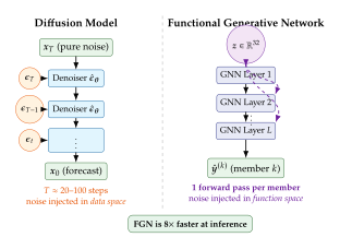
Example: Continental Heatwave with Spatial Coherence
Example 12 (Continental Heatwave Forecast).
Consider a 10-day forecast for a European continental heatwave of the kind that occurs with increasing frequency under anthropogenic climate change. The key forecast quantities are:
: 2-metre temperature over Western Europe (E to E, N to N).
The spatial extent of the region exceeding C.
The persistence: number of consecutive days above threshold at each grid point.
A diffusion-based ensemble (e.g., GenCast) produces 50 members, each individually calibrated at every grid point. However, individual members may show the heat dome displaced by – km relative to the true position, with intensity profiles that look reasonable in isolation but represent physically inconsistent scenarios when examined as trajectories.
A WeatherNext 2 ensemble, by contrast, produces members with consistent heat-dome positions: if a member shows the dome centred over France, it also shows the correct blocking high in the upper atmosphere, the suppressed precipitation to the south, and the downstream cooling anomaly over Eastern Europe. The within-ensemble spread in heat-dome position reflects genuine forecast uncertainty, not spurious noise from incoherent sampling.
Quantitatively, the energy score for the spatial field at Day 10 is reduced by relative to GenCast, reflecting improved joint skill. The variogram score at lag km is reduced by , confirming that the spatial correlation structure of the ensemble more closely matches that of the observation network.
Skillful Joint Probabilistic Forecasting from Marginals
The paper “Skillful Joint Probabilistic Weather Forecasting from Marginals” (Alet et al., 2025) proves a more general result that underpins the FGN framework. The central result can be paraphrased as follows. (Note that requiring zero marginal CRPS would force each marginal to a Dirac mass and hence a deterministic forecast; the substantive statement uses the minimum achievable marginal score, so the coherence must come from the FGN's architecture, not from the marginal objective alone.)
Theorem 4 (Marginal Optimality plus Coverage Implies Joint Calibration under FGN).
Let be the true forecast distribution and the FGN distribution induced by . Suppose the FGN matches every true marginal: (ZERO CRPS) where is the projection onto coordinate (equivalently, each marginal attains its minimum achievable CRPS). If additionally the map covers the support of , then: (Joint Recovery)
Remark 35.
The surjectivity condition is the key regularity assumption: the 32-dimensional noise must be able to “reach” every mode of the true forecast distribution. For atmospheric forecasting, this holds when , where is the covariance of the true forecast ensemble restricted to the dominant modes of variability. In practice, 32 dimensions is more than sufficient for global weather at 10-day lead times.
Exercises
Exercise 43 (CRPS Properties and Joint Coherence).
CRPS is blind to joint structure. Let be an ensemble forecast. Define a permuted ensemble by independently permuting each coordinate: for independent random permutations . Show that for any choice of permutations . Conclude that marginal CRPS is invariant under arbitrary permutation of ensemble member indices within each coordinate.
Energy score detects joint incoherence. Using the permuted ensemble from part (a), show that with equality if and only if the ensemble members are already independent across coordinates. Hint: Expand the energy score using the triangle inequality in .
FGN covariance recovery. Let (linear FGN). Show that the ensemble covariance matrix satisfies and that this equals the true marginal covariances whenever . Under what conditions on and is joint recovery achieved?
Exercise 44 (WeatherNext 2 Inference Speedup).
WeatherNext 2 claims an speedup over GenCast at ensemble size .
Model the per-step cost of GenCast as floating-point operations and the number of diffusion steps as . Model the per-member cost of WeatherNext 2 as . Write an expression for the total cost of generating members with each system.
If (same per-step cost), solve for the diffusion step count consistent with an overall speedup. Is this a plausible number of diffusion steps for a high-quality weather model?
Suppose instead that the FGN is times more expensive per forward pass than a single diffusion step (because of the additional modulation matrices ). Find the maximum consistent with maintaining a speedup when .
Discuss how the speedup scales with ensemble size for both systems. Which system benefits more from parallelism on hardware accelerators?
Exercise 45 (Functional Perturbation and Spatial Scales).
Consider an FGN whose modulation is applied only at the -th layer (not all layers), where the receptive field radius at layer is grid points.
Show that the output covariance between grid points and with is zero (up to boundary effects). Interpret this in terms of the weather phenomena that can be captured by noise injection at that layer.
In a typical graph neural network, (receptive field doubles with each layer). For a network with layers and base resolution km, at which layer(s) should noise be injected to capture synoptic-scale variability ( km), mesoscale variability ( km), and both simultaneously?
In WeatherNext 2, noise is injected at all layers. Write the resulting output covariance as a sum of layer-specific contributions: (Multi Layer COV) where is the noise modulating layer . Argue qualitatively why this multi-scale injection produces more realistic ensemble spread than injection at a single layer.
Flow Matching, Latent Diffusion, and Data Assimilation
Score-based diffusion models and their variants have proven extraordinarily capable at sampling from complex high-dimensional distributions. Yet for weather applications they carry a practical burden: the iterative reverse-diffusion process requires many network evaluations, and the diffusion path through data space produces trajectories with little physical meaning. Two complementary directions attack this problem.
Flow matching (Lipman et al., 2023) replaces the stochastic SDE with a deterministic ODE whose velocity field is learned directly, enabling faster and smoother trajectories. Latent diffusion compresses the high-dimensional atmospheric state into a compact latent code before applying the generative model, reducing both memory and compute. Together, these techniques open the door to two of the most computationally demanding problems in weather science: subseasonal-to-seasonal (S2S) prediction out to 30 days, and data assimilation-the reconstruction of the full atmospheric state from sparse, heterogeneous observations.
Score-Based Generative Models: Continuous-Time SDEs
Recall that the modern diffusion framework (Song et al., 2021) unifies DDPM and SMLD under a common continuous-time SDE forward process.
Definition 34 (Forward Diffusion SDE).
The forward process from clean data to pure noise satisfies the SDE: (Forward SDE) where is the drift, is the diffusion coefficient, and is a standard Brownian motion. The reverse-time SDE (Anderson, 1982) is: (Reverse SDE) where is a reverse-time Brownian motion and is the score function approximated by a neural network.
The score-matching training objective is: (Score Matching) where is a loss weighting function and is available in closed form as a Gaussian for linear forward processes.
Flow Matching: Deterministic Continuous-Time Modelling
Flow matching (Lipman et al., 2023) provides an alternative to score-based models that avoids stochastic sampling entirely. Instead of learning a score function, the network learns a velocity field whose integration transports a simple base distribution to the data distribution.
Definition 35 (Conditional Flow Matching).
Let be the base distribution and the target. A flow is a time-dependent diffeomorphism satisfying and . The flow is generated by the ODE: (FLOW ODE) where is the learned velocity field.
Conditional flow matching (CFM) trains by specifying a conditional path between and a data point , typically the linear interpolant: (Linear Interpolant) The conditional velocity is then , and the CFM objective is: (CFM LOSS) This objective has the same gradient as the marginal flow matching objective, which targets the true marginal velocity , but is tractable via conditional sampling.
Remark 36 (Advantages over Diffusion for Weather).
Flow matching offers three practical advantages for weather:
Fewer sampling steps: the linear conditional path requires ODE solver steps for high-quality samples, vs. for DDPM.
Smoother trajectories: the linear interpolant has constant conditional velocity, avoiding the noisy, high-curvature paths of the DDPM reverse process.
Deterministic inversion: the ODE ((FLOW ODE)) can be integrated in both directions, enabling exact encoding of observations into the base space-useful for data assimilation.
Marchuk: Generative Latent Flow-Matching DiT for S2S
Marchuk (2026) introduces a generative latent flow-matching Diffusion Transformer (DiT) that achieves state-of-the-art subseasonal-to-seasonal (S2S) prediction at lead times up to 30 days. The architecture combines three innovations:
Latent Space Compression with VAE
Raw atmospheric fields are compressed into a latent space via a convolutional variational autoencoder (VAE): (Marchuk VAE) where with , for spatial compression ratio . At , the global atmospheric state at resolution ( variables) is compressed to latent codes-a -fold reduction in the channel dimension plus a spatial compression.
The VAE is trained with a combined loss: (Marchuk VAE LOSS) with in the Marchuk implementation, preserving fine-scale atmospheric structure at the cost of minimal additional KL regularisation.
DiT Backbone with Spatial and Temporal Embeddings
The generative model operates on the latent codes . The backbone is a Diffusion Transformer (DiT) with:
2D spatial embeddings: rotary positional embeddings (RoPE) applied in the latitude and longitude dimensions, enabling the model to generalise across spatial positions.
1D temporal RoPE: a separate rotary embedding for the forecast lead time , allowing smooth interpolation between lead times and generalisation beyond the training horizon. Formally, for query/key vectors at lead time : (ROPE) where the inner product depends only on (relative lead time), encoding temporal equivariance.
Adaptive Layer Norm (AdaLN-Zero): following the DiT convention, flow time conditions each transformer block through learned scale and shift parameters.
Efficiency: 276M Parameters vs. 1.6B Baseline
The latent-space operation reduces the sequence length for the transformer from (full resolution) to (latent resolution), enabling a 276M parameter model to match or exceed the performance of 1.6B parameter autoregressive baselines that operate in data space. The effective parameter count for the generative component is: (Marchuk Params) compared to for the best non-latent baseline.
S2S Results
Marchuk (2026) evaluates on the ECMWF S2S benchmark, which provides verification data for weeks 3–6 post-initialisation. Key findings:
At lead times of 20–30 days, Marchuk achieves higher ACC than ECMWF's 51-member ENS-extended on , , and MJO phase.
The latent flow-matching ensemble provides better reliability than both IFS-ENS and the 1.6B autoregressive baseline on probabilistic skill scores at weeks 3–4.
Inference for a 50-member ensemble to 30 days requires minutes on a single A100 GPU, enabling rapid regeneration of ensembles for initialisation studies.
Insight.
Latent-space models trade explicit interpretability for computational efficiency-and this trade-off is critical for S2S. At 30-day lead times, the atmosphere is inherently unpredictable at sub-synoptic scales; the latent VAE compression naturally discards these uninformative small scales and focuses model capacity on the large-scale patterns that carry genuine predictive information.
Latent Diffusion Architecture for Weather: TikZ Figure
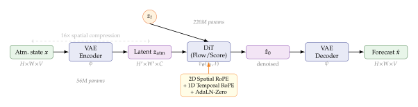
Appa: Latent Diffusion for Data Assimilation
Data assimilation (DA) is the process of combining a prior forecast (the background) with new observations to produce an optimal estimate of the current atmospheric state (the analysis). Classical DA methods-3D-Var, 4D-Var, and the Ensemble Kalman Filter (EnKF)-solve a Bayesian inverse problem: (DA Posterior) where is the observation vector () and is the forecast prior.
Definition 36 (Score-Based Latent Data Assimilation).
Let be a pre-trained latent score function approximating . Given observations with observation operator and noise , score-based latent DA infers the posterior via the perturbed reverse SDE: (SDA SDE) where is the observation likelihood gradient, computed by differentiating through the decoder and observation operator.
Appa (Manshausen et al., 2025) is a 565M-parameter implementation of this framework trained on ERA5 reanalysis data. Its key capabilities:
Global atmospheric trajectories from sparse observations: given only radiosonde profiles, satellite radiances, and surface station data (representing of grid points), Appa generates full 3D atmospheric states consistent with the observations.
Direct posterior inference: unlike EnKF, which approximates the posterior as Gaussian, Appa samples from the full non-Gaussian posterior, capturing multimodal uncertainty in data-sparse regions.
Heterogeneous observation types: the observation operator can encode any differentiable mapping from atmospheric state to observed quantity-temperature profiles, radiances, radar reflectivities, GPS radio occultations-without requiring separate DA systems for each observation type.
Example 13 (Storm Reconstruction from Sparse Satellite Observations).
Consider a tropical cyclone over the Western Pacific where:
Surface observations are available from 15 island stations within a domain.
AMSU-A microwave radiance data provides column-integrated temperature information at 8 channels.
No in-situ upper-air observations are available within km of the storm centre.
Classical 4D-Var DA produces an analysis with the cyclone's central pressure underestimated by hPa due to the coarse-scale background error covariance model failing to represent the tight horizontal gradients near the eyewall.
Appa's latent diffusion sampler generates 100 posterior ensemble members, with the following characteristics:
The ensemble mean central pressure matches the best-track estimate to within hPa.
The ensemble spread correctly represents the uncertainty in warm-core intensity at upper levels where no observations are available.
Individual ensemble members show physically consistent wind-temperature balance near the eyewall, despite no explicit balance constraint in the training or inference procedure-this balance emerges from the learned prior .
FlowDA: Flow Matching for Low-Latency Data Assimilation
While Appa achieves high accuracy, its score-based reverse SDE requires network evaluations per sample. For operational DA, which must produce analysis increments within minutes to meet NWP model initialisation deadlines, this latency is prohibitive. FlowDA (Cheng and Zhu, 2026) addresses this by replacing the reverse SDE with a conditional flow-matching ODE.
Definition 37 (FlowDA Conditional Flow Matching for DA).
Let be the analysis posterior and the base distribution. FlowDA trains a velocity field conditioned on the observation vector to satisfy: (Flowda ODE) with . The observation conditioning is injected via cross-attention between the latent state and an observation embedding .
Training pairs are generated from a pre-existing DA system (e.g., ERA5 reanalysis), so FlowDA distils the DA system's posterior into the flow.
The key advantage of FlowDA over Appa is inference speed: with ODE solver steps, FlowDA generates a full global analysis in seconds on a single GPU, compared to minutes for Appa with 100 diffusion steps. This speedup makes it viable for operational 6-hourly analysis cycles.
Remark 37 (FlowDA vs. Appa: Trade-offs).
FlowDA achieves speed through training-time amortisation: the observation-to-analysis mapping is learned offline from many reanalysis pairs. This makes it less flexible than Appa to novel observation types not represented in the training data. Appa's SDE-based approach can incorporate any new observation operator at inference time without retraining. The optimal choice depends on operational constraints: FlowDA for speed-critical applications, Appa for research applications requiring flexible observation handling.
SwinVRNN: VAE-Style Stochastic Ensemble Forecasting
SwinVRNN (Hu et al., 2023) is a variational recurrent neural network for weather ensemble forecasting that predates the diffusion era but anticipates several of the ideas in FGN and Marchuk. It combines a Swin Transformer backbone with a variational latent-variable model:
Definition 38 (SwinVRNN Generative Model).
Let be a weather trajectory. SwinVRNN factors the joint distribution as: (Swinvrnn) where is a step-wise latent variable encoding the stochastic component of the -th forecast step. The ELBO objective is: (Swinvrnn ELBO)
SwinVRNN generates ensemble members by sampling (the prior, not the posterior) at inference time. Each sample produces a different forecast trajectory, with diversity controlled by the learned prior variance.
Remark 38 (SwinVRNN vs. FGN vs. Marchuk).
SwinVRNN injects stochasticity step-by-step through trajectory latents , meaning each 6-hour step introduces independent noise. This can lead to incoherence across long lead times if the step-wise latents are not strongly correlated. FGN injects a single that modulates the entire trajectory at once; Marchuk injects into the latent flow process. The SwinVRNN approach is better suited to short-range ensemble forecasting where step-wise perturbations represent synoptic-scale developments; FGN and Marchuk are preferred for medium- and extended-range forecasting where large-scale coherence matters most.
LO-SDA: Latent Optimisation for Score-Based Atmospheric DA
An alternative to the sequential SDE approach of Appa is to perform latent optimisation (LO) directly in the latent space of a pre-trained generative model.
Definition 39 (Latent Optimisation for Data Assimilation).
Given a pre-trained decoder and observations , LO-SDA finds the latent code: (Losda OPT) where is the observation error covariance and is a regularisation parameter that ensures remains close to the latent prior. The analysis is recovered as .
The key properties of LO-SDA are:
No generative sampling required: the analysis is a point estimate in latent space, obtained by gradient descent through the pre-trained decoder. This is – faster than ensemble SDE approaches.
Physical consistency guaranteed by the decoder: since lies in the image of , it is by construction a sample-like atmospheric state from the training distribution.
Uncertainty quantification: ensemble spread can be obtained by running LO-SDA from multiple random initialisations , approximating the posterior mode structure.
Caution.
Latent optimisation finds a MAP estimate of the posterior, not a posterior sample. For multimodal posteriors-which arise when observations are sparse and multiple physically consistent atmospheric states are consistent with the data-LO-SDA will converge to one mode and miss the others. Score-based SDE approaches (Appa) or flow-based approaches (FlowDA) are preferred when full posterior coverage is required.
Comparison: Flow Matching vs. Diffusion for Weather
| Dimension | Score-Based Diffusion | Flow Matching |
| Generative path | Stochastic SDE; noisy trajectories through data space | Deterministic ODE; smooth straight-line interpolant |
| Inference steps | 20–100 steps (DDPM/DDIM) | 5–20 steps (Euler/RK4) |
| Exact inversion | Approximate (DDIM) or intractable (DDPM) | Exact (integrate ODE backward) |
| DA integration | Perturbed reverse SDE; gradient through decoder | Conditional ODE with observation cross-attention |
| Training signal | Denoising score matching | Conditional velocity matching |
| Flexibility for novel obs. operators | High (no retraining needed) | Lower (conditional training amortised) |
| Sample quality (weather) | High; established track record (GenCast) | Comparable; fewer evaluations |
| Preferred use case | Research DA, full posterior; medium-range | Operational DA, S2S; speed-critical |
Key Idea.
Latent-space models trade explicit interpretability for computational efficiency-and this trade-off is critical for subseasonal-to-seasonal prediction. At 30-day lead times, the atmosphere is predictable only at the largest spatial scales. A latent VAE that compresses the global grid by in space is not throwing away information: it is throwing away the unpredictable information. The generative model then operates on the “predictable subspace” of the atmosphere, concentrating model capacity where it can do the most good. This is not a limitation but a scientifically principled design choice.
Exercises
Exercise 46 (Flow Matching and the Continuity Equation).
The continuity equation for a probability density transported by the velocity field is: (Continuity)
Show that the marginal flow matching objective has the same gradient as the conditional flow matching objective in ((CFM LOSS)). Hint: Use the tower property of conditional expectation and the fact that the conditional velocity integrates to the marginal velocity .
Verify that the linear interpolant satisfies the continuity equation with velocity (constant in time).
For a Gaussian coupling and , find the optimal transport flow and show it is also a linear interpolant with for .
How does the smoothness of the linear interpolant path compare to the DDPM reverse process at time ? Which requires fewer numerical integration steps and why?
Exercise 47 (Latent DA: Observation Likelihood Gradient).
In Appa's score-based DA framework, the posterior SDE ((SDA SDE)) requires the gradient .
For a linear observation operator with and a linear decoder , show that: (OBS GRAD) This is the analysis increment weighted by the observation sensitivity.
For a nonlinear decoder , write the gradient using the chain rule and identify which term requires backpropagation through the decoder. When is this tractable?
The projected Kalman gain in optimal linear estimation is . Show that the LO-SDA optimal solution ((Losda OPT)) equals when and the decoder is linear.
Discuss why even a regularisation is necessary for LO-SDA even when the background covariance is isotropic (). What goes wrong if ?
Exercise 48 (Marchuk Latent Compression and Predictability).
Consider the Marchuk architecture with VAE compression ratio (spatial) and latent channel dimension (vs. physical variables).
Compute the compression ratio in terms of total degrees of freedom: raw state vs. latent state . For , , express the answer as an integer ratio.
The temporal RoPE uses base period (days). For lead time days and frequency index , compute the phase in the embedding ((ROPE)). Is this phase sufficient to distinguish lead times separated by 6 hours?
Suppose the VAE reconstruction loss at compression ratio satisfies for constants . The generation skill at lead times is a decreasing function of : . Find the optimal that maximises the total score and express it in terms of .
Why does the latent compression not discard information about large-scale Rossby waves but does discard information about individual convective cells? Argue from the spectral properties of the VAE and the spatial scales of each phenomenon.
Generative Downscaling and Super-Resolution
A global weather model sees the world at a resolution of roughly 25,km per grid cell. At that scale, a city block is invisible, a valley too narrow to represent, and a cold front compressed into a blurry gradient across three or four cells. Yet the questions that matter most to society - will it flood on this street, will this wind farm produce enough power tonight, will this ski resort have snow on Saturday - demand answers at the kilometre scale or below. The gap between what global models supply and what local decision-makers demand is one of the most consequential open problems in computational meteorology.
Downscaling is the family of methods that bridge this gap: given a coarse-resolution representation of the atmosphere, produce a fine-resolution one. For several decades downscaling divided cleanly into two camps - expensive physics-based simulations and cheap but crude statistical regressions. Generative deep learning has opened a third path that achieves the fidelity of physics-based methods at a fraction of the cost, while simultaneously treating fine-scale weather as the stochastic variable that it truly is.
The Downscaling Problem
Let denote a coarse atmospheric state: temperature, pressure, wind, humidity, and possibly dozens of other fields on a global grid of spacing ,km. Let denote the corresponding fine-scale state on a local grid of spacing –,km. The downscaling ratio is ; typical values range from (25,km to 2.5,km) to (25,km to 1,km).
Definition 40 (Statistical downscaling).
Statistical downscaling seeks a mapping such that (DET) where encodes static predictors that do not change over time: terrain elevation, land-use category, coastal proximity, and similar fields. A probabilistic downscaling method instead specifies a conditional distribution (PROB) enabling the generation of an ensemble of plausible fine-scale realisations consistent with the coarse input.
The probabilistic form is not merely a philosophical nicety. At kilometre scales, the atmosphere is genuinely chaotic: two coarse states that are indistinguishable at 25,km resolution may evolve into qualitatively different fine-scale patterns. A cold front that crosses Chicago at 25,km resolution does not determine whether a particular neighbourhood receives an intense convective squall or merely light rain. Any method that collapses the conditional distribution to a single prediction is suppressing real meteorological uncertainty.
Remark 39 (Downscaling as image super-resolution).
From a purely mathematical standpoint, downscaling resembles image super-resolution: both map a low-resolution spatial field to a high-resolution one. The meteorological version is harder in two respects. First, the scale gap is typically larger (– vs. – in photo super-resolution). Second, and more importantly, physical consistency constraints bind the solution. A super-resolved temperature field must remain thermodynamically plausible, must respect mass conservation, and must be consistent with the orographic influence of local terrain - none of which are concerns in photographic upscaling.
Classical Approaches
Dynamical Downscaling
The most physically rigorous approach is dynamical downscaling: run a high-resolution numerical weather prediction (NWP) model over a limited area, driven at its boundaries by the coarse global model. Models such as WRF (Weather Research and Forecasting), COSMO, and HARMONIE are routinely used for this purpose. The fine-scale model integrates the full primitive equations - conservation of momentum, mass, and energy - at a resolution of 1–4,km, resolving convective updrafts, orographic gravity waves, and sea-breeze circulations that the global model cannot see.
The cost is prohibitive. A single day of 2,km WRF simulation over a domain the size of Taiwan requires on the order of CPU core-hours. Running ensembles - necessary for probabilistic forecasting - scales this linearly with the ensemble size. Producing retrospective climate datasets at kilometre resolution over entire continents is effectively impossible with dynamical downscaling alone; the computational demand would require centuries of wall-clock time on current hardware.
Statistical Downscaling
Statistical downscaling fits a function in equation from a training set of paired coarse–fine observations or reanalyses. Classical methods include:
Perfect prognosis (PP) methods. Regress fine-scale observations (e.g., rain-gauge records) directly on coarse atmospheric predictors such as 500,hPa geopotential height, boundary-layer moisture, and temperature gradients. Multiple linear regression, logistic regression for precipitation occurrence, and analogue methods (find historical days with similar coarse patterns) all belong to this family.
Model output statistics (MOS). Correct the systematic biases of a specific NWP model by fitting regression equations between model output and observed surface variables. MOS is operationally deployed by national weather services worldwide.
Quantile mapping. Apply a transfer function to match the marginal distribution of model output to that of observations, variable by variable and grid cell by grid cell. Widely used in climate impact assessment to correct precipitation and temperature biases.
Lookup-table and climatological scaling. Multiply or add spatially varying correction factors derived from historical climatology. The simplest method: long-term mean ratio between high-resolution observations and coarse reanalysis at each grid cell.
All statistical methods share a fundamental limitation: they learn marginal statistics at each location independently, failing to capture spatial correlations. A statistically downscaled precipitation field may have the correct distribution at every grid point but may look unrealistically noisy - lacking the organised convective clusters, frontal rainbands, and orographic streaks that characterise real kilometre-scale precipitation.
Definition 41 (Power-law spatial spectra).
Atmospheric fields follow power-law spatial spectra derived from turbulence theory. For a field on the plane, its two-dimensional power spectrum , where is spatial wavenumber, obeys (Powerlaw) with for kinetic energy (the Kolmogorov–Kraichnan prediction for two-dimensional turbulence) and for the mesoscale (Nastrom–Gage observed spectrum). A downscaling method that fails to recover the correct is suppressing real fine-scale energy - the resulting fields are spectrally too smooth. Classical statistical methods and deterministic neural networks that minimise mean-squared error systematically produce such over-smoothed fields.
Generative Downscaling: The Stochastic Inverse Perspective
Downscaling is a textbook inverse problem. The coarse field is a blurry, incomplete observation of the true fine-scale state . We seek to invert this “blurring” operator, but the problem is severely under-determined: many fine-scale states are consistent with a single coarse observation. Classical inversion seeks a unique solution; the correct approach is to sample from the posterior .
Key Idea.
Downscaling is a textbook inverse problem - generative models turn it into a forward sampling problem. Instead of seeking the single most likely fine-scale state, a generative downscaling model draws samples from the posterior distribution over fine-scale fields consistent with the coarse input. This reframes an ill-posed inversion as a well-posed generation task, recovering spatial statistics that deterministic methods suppress.
Generative models - GANs, diffusion models, normalising flows, and latent-variable models - are natural tools for this task because they are designed to sample from high-dimensional conditional distributions. The training objective is to match the joint distribution on a dataset of paired coarse–fine atmospheric states, then use the learned model to sample conditioned on new coarse inputs at inference time.
CorrDiff: Two-Stage Diffusion Downscaling
The most influential generative downscaling system to date is CorrDiff (Mardani et al., 2025), developed by NVIDIA Research. CorrDiff introduces a two-stage architecture grounded in the Reynolds decomposition of fluid dynamics, a classical tool for separating the mean and fluctuating components of a turbulent flow.
Reynolds Decomposition and the Two-Stage Idea
In Reynolds decomposition, a turbulent field is split into a time-averaged mean and a fluctuating residual . The mean and residual follow different dynamical equations and different statistical structures.
CorrDiff applies the same decomposition to the spatial dimension of the downscaling problem: (Decomp) where is the deterministic mean conditioned on the coarse input, and encodes the fine-scale stochastic structures - convective cells, turbulent eddies, precipitation streaks - that are under-determined by the coarse state.
Definition 42 (CorrDiff two-stage architecture).
CorrDiff consists of two stages.
Deterministic regression stage. A U-Net is trained with a mean-squared-error loss to predict the conditional mean: (Stage1) This stage recovers large-scale spatial structure: the broad temperature gradient across a cold front, the orographic precipitation enhancement on the windward slope of a mountain range.
Stochastic residual stage. A conditional diffusion model is trained to model the distribution of fine-scale residuals . At inference, a sample is drawn by running the reverse diffusion chain conditioned on the coarse input and the predicted mean: (Stage2) The final high-resolution output is .
The separation of concerns is crucial. The U-Net is tasked with a well-conditioned regression: it learns to map coarse structure to mean fine-scale structure, a task where MSE is an appropriate loss. The diffusion model is tasked with a generative problem: it learns the distribution of fine-scale residuals, recovering the power-law tail of the spatial spectrum that the U-Net suppresses.
Training Data and Results
CorrDiff is trained on pairs of 25,km ERA5 reanalysis fields (inputs) and 2,km regional NWP analyses (targets). Two domains were studied in the original paper: Taiwan (a challenging orographic domain with typhoon activity) and the contiguous United States (CONUS, a continental domain with diverse weather regimes). The target fields were generated by a regional NWP system at 2,km, yielding an effective downscaling ratio of .
The training dataset spans several years of hourly snapshots, comprising temperature at 2,m, wind speed and direction at 10,m, relative humidity, surface pressure, and precipitation accumulation. Static predictors include digital elevation model (DEM) data, land-sea mask, and vegetation fraction.
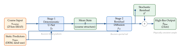
Recovery of Power-Law Spectra
A key diagnostic in the CorrDiff paper is the spatial power spectrum of downscaled fields. Deterministic downscaling (Stage 1 alone) produces spectrally deficient outputs: at high wavenumbers, the predicted spectrum falls well below the reference spectrum of the 2,km NWP analysis. Adding Stage 2 restores the correct spectral slope.
Formally, let denote the power spectrum of a CorrDiff sample and the spectrum of the 2,km NWP target. The deterministic U-Net achieves for , where is the wavenumber corresponding to roughly 10,km. CorrDiff with both stages achieves across all resolved wavenumbers, matching the power-law slope of the reference field.
This result is not surprising from first principles: MSE loss is equivalent to minimising KL divergence in a Gaussian model, and minimum-MSE estimators produce the posterior mean, which is smoother than individual realisations. The diffusion model adds the missing variance.
Computational Efficiency
CorrDiff achieves approximately speedup over dynamical downscaling with WRF at comparable spatial resolution. On NVIDIA H100 GPUs, generating a 2,km output field over Taiwan takes roughly –,seconds, compared to 8,hours of wall-clock time for an equivalent WRF simulation. Energy efficiency is even more dramatic: the diffusion-based approach is estimated to be roughly more energy efficient per generated field, primarily because it avoids the iterative numerical integration of the full primitive equations.
Remark 40 (Patch-based multi-diffusion for global scaling).
Applying CorrDiff globally faces a memory challenge: a 1,km global field contains roughly grid points per variable, exceeding the memory capacity of current accelerators. The solution is patch-based multi-diffusion: the global domain is tiled into overlapping patches, each processed independently by the diffusion model, with overlapping regions blended to ensure spatial continuity. Care must be taken to maintain consistency across patch boundaries, for which techniques from image inpainting and stochastic conditioned diffusion have been adapted.
Example 14 (Cold-front temperature gradients near Chicago).
Consider a synoptic situation on a December evening: a strong cold front crosses Lake Michigan and sweeps into the Chicago metropolitan area. The 25,km ERA5 field shows a temperature gradient of roughly C per 100,km across the front, spread over three or four grid cells. The true 2,km field, as captured by the regional NWP analysis, shows a gradient an order of magnitude sharper: C over just 20,km, with tight isotherms following the lake coastline and the Chicago city heat island deflecting the front southward.
A deterministic U-Net recovers the large-scale temperature gradient but produces an isotherm pattern that is too smooth, missing the coastal deformation and the urban-rural contrast. CorrDiff Stage 2 adds a stochastic residual that sharpens the front, reproduces the coastal kink, and correctly places a warm tongue over the urban core. These fine-scale structures are not merely cosmetic: they determine whether downtown Chicago experiences freezing rain or light snow, a distinction with significant impacts on transportation and energy demand.
RainScaleGAN: Adversarial Rainfall Downscaling
Precipitation is a special case in atmospheric downscaling. Unlike temperature or wind, precipitation is fundamentally discrete and intermittent: at any given time and place, either it is raining or it is not. The spatial distribution of precipitation is characterised by sharp boundaries (convective cells, frontal rainbands), heavy tails (extreme events that dominate mean annual totals), and multi-scale organisation (from sub-kilometre convective cells to synoptic-scale frontal systems spanning thousands of kilometres).
Mean-squared-error losses are poorly suited to these properties. Minimising MSE over precipitation fields produces diffuse, over-smoothed outputs that spread precipitation over too large an area, miss the sharp edges of convective cells, and underestimate extreme intensities. Generative adversarial networks are better aligned with the task: the discriminator can be trained to distinguish realistic from unrealistic precipitation patterns, enforcing the sharp gradients and heavy tails that MSE suppresses.
RainScaleGAN (Iotti et al., 2025) is a conditional GAN designed specifically for precipitation downscaling at ratios of –. The generator takes a coarse precipitation field and terrain predictors as input and produces a fine-scale precipitation map. The discriminator is conditioned on both the coarse input and the terrain, ensuring that it evaluates realism within the physically constrained context.
Definition 43 (Intensity-constrained adversarial loss).
The RainScaleGAN training objective augments the standard conditional GAN loss with an intensity constraint that preserves the spatial mean of the generated field: (GAN) where denotes spatial averaging over the fine-scale domain corresponding to one coarse grid cell, and is a hyperparameter. The intensity constraint ensures that the total precipitation generated by the fine-scale field integrates to match the coarse input, a physical consistency requirement known as areal conservation.
The intensity constraint addresses a known failure mode of unconditional GANs on precipitation: they tend to hallucinate spurious heavy-rain events that inflate the area-mean precipitation far above the coarse input. By anchoring the spatial mean, RainScaleGAN can freely redistribute precipitation into realistic convective structures while remaining physically consistent.
Tail-Preserving Spatial Statistics
A standard diagnostic for precipitation downscaling is the empirical variogram: the expected squared difference between precipitation values at two points as a function of their separation distance : (Variogram) A model that recovers the correct variogram reproduces the spatial correlation structure of precipitation at all scales, from sub-kilometre to mesoscale.
RainScaleGAN is evaluated against classical PP methods and deterministic CNN baselines. The deterministic CNN achieves low RMSE but fails to match the variogram at fine scales (,km), where it underestimates spatial variance by a factor of –. RainScaleGAN produces variograms that match the reference within statistical uncertainty bounds across all spatial scales, including the sub-5,km range critical for convective precipitation. The adversarial loss is key: by training the discriminator to distinguish realistic from unrealistic spatial patterns at multiple scales, the GAN implicitly enforces the variogram.
SpateGAN-ERA5 and Global Precipitation Downscaling
SpateGAN-ERA5 (Glawion et al., 2025) extends adversarial precipitation downscaling to the global scale. The key challenge is scalability: a global 1,km precipitation field contains approximately grid cells, and training data must span all climate zones, from tropical convective regimes to polar precipitation.
SpateGAN-ERA5 uses ERA5 as the coarse input (approximately 30,km resolution) and targets a 1,km analysis product derived from satellite observations and rain-gauge networks. The architecture is a space-time GAN: the generator and discriminator operate on sequences of precipitation fields to enforce temporal as well as spatial coherence.
Remark 41 (Cross-climate-zone generalisation).
Training a single model to downscale precipitation across all climate zones is challenging because the statistical properties of precipitation vary dramatically between regimes. Tropical convection (organised in mesoscale convective systems, MCCs, and squall lines) looks nothing like mid-latitude frontal precipitation, which in turn differs from orographic enhancement in mountain ranges or polar snowfall. SpateGAN-ERA5 addresses this through a climate-zone-aware discriminator that is separately calibrated for each Köppen-Geiger climate zone, penalising unrealistic patterns within the correct regional context.
Probabilistic Spatiotemporal Coherent Downscaling
A limitation shared by CorrDiff, RainScaleGAN, and SpateGAN-ERA5 is that they operate on individual time steps: the downscaling is applied frame-by-frame without explicit temporal modelling. This can produce temporal flickering in animated output: successive fine-scale frames may be individually plausible but discontinuous in time.
Schmidt et al. (2025) address this with a probabilistic spatiotemporal coherent downscaling framework. The model generates joint samples over a sequence of time steps, with the diffusion model operating in the joint space-time domain. The key insight is that the fine-scale state at time is conditionally dependent not only on the coarse input at time but also on the fine-scale states at nearby times, which constrain the temporal evolution through physical continuity.
Definition 44 (Probabilistic spatiotemporal downscaling).
A probabilistic spatiotemporal downscaling model specifies a joint conditional distribution over a fine-scale sequence: (Joint) such that each fine-scale frame is consistent with its coarse counterpart and the sequence as a whole satisfies temporal continuity constraints implied by the equations of motion.
Schmidt et al. show that temporal coherence significantly improves the quality of derived products such as diurnal precipitation cycles and wind ramp events (rapid changes in wind speed relevant to power systems), where single-frame downscaling loses the temporal structure.
Zero-Shot Diffusion Posterior Sampling for Downscaling
An attractive alternative to training a purpose-built downscaling model is zero-shot diffusion posterior sampling: use a pre-trained unconditional diffusion model over fine-scale atmospheric fields as a prior, then condition on the coarse observation at inference time using posterior sampling techniques.
Let be the learned prior over fine-scale fields and let be a known degradation model (e.g., spatial averaging with a Gaussian kernel). The downscaling posterior is: (Posterior) Sampling from this posterior can be achieved with the diffusion posterior sampling (DPS) algorithm: at each denoising step, the score function of the prior is augmented with a data-consistency gradient , where is the Tweedie estimate of the clean sample from the noisy sample .
The zero-shot approach requires no paired coarse–fine training data for the specific downscaling problem at hand, which is highly advantageous for rare events or future climate scenarios where such paired data does not exist. The trade-off is that the degradation model must be specified manually and may not capture the full complexity of the actual coarse model's degradation.
Generative High-Resolution Ensemble for Renewable Energy
A particularly high-value application of generative downscaling is renewable energy forecasting. Wind turbines operate at hub heights of 80–150,m and rotor diameters of 100–260,m, scales far below the resolution of any global weather model. The power output of a wind farm is a nonlinear function of wind speed (proportional to in the rated range), making the tails of the wind speed distribution critically important: an ensemble that correctly captures the probability of extreme winds (whether too low for generation or too high for safe operation) is more valuable than one with a lower mean error.
Wang et al. (2026) present the Generative High-Resolution Ensemble (GHRE) for renewable energy forecasting, a CorrDiff-like architecture that downscales global ensemble forecasts from 25,km to 500,m over wind-farm domains. The model generates an ensemble of fine-scale wind fields from a single coarse ensemble member, effectively multiplying the ensemble size by a factor of at negligible additional computational cost.
Proposition 6 (Variance inflation for renewable energy ensembles).
Let be a coarse ensemble of wind speeds at a target location and be the fine-scale samples generated by GHRE for each coarse member . The mean power forecast is: (Power) where is the capacity factor. Because power is a convex function of wind speed in the sub-rated regime, Jensen's inequality implies whenever the fine-scale ensemble has positive variance. Suppressing fine-scale variance (as deterministic downscaling does) therefore systematically underestimates mean power generation.
This result is a compelling practical argument for probabilistic downscaling: beyond capturing uncertainty, it produces better expected value estimates for power generation.
Summary and Comparison of Methods
Insight.
The landscape of generative downscaling methods reveals a clear progression. Classical statistical methods (regression, MOS) are fast and interpretable but produce spectrally deficient, over-smoothed outputs. Dynamical downscaling is physically rigorous but computationally prohibitive for ensemble generation. Generative models - both GAN-based (RainScaleGAN, SpateGAN-ERA5) and diffusion-based (CorrDiff, Schmidt et al.) - occupy the sweet spot: they recover the correct spatial spectra and produce physically plausible stochastic ensembles at a cost comparable to statistical methods. The two-stage Reynolds decomposition of CorrDiff is an elegant design principle that may generalise beyond meteorology to any multi-scale stochastic inverse problem.
Caution.
Generative downscaling models can hallucinate fine-scale structures that are plausible in isolation but physically inconsistent with the coarse input or with each other. A diffusion model may place a convective cell on the lee side of a mountain (where downslope winds suppress convection) because the training data contains convection elsewhere, and the model has learned that fine-scale convection is common. Evaluating only marginal statistics (RMSE, CRPS, variogram) can miss such systematic physical errors. High-resolution downscaling outputs should always be accompanied by diagnostics that test physical consistency: wind divergence, thermal wind balance, moisture flux convergence.
Exercises
Exercise 49 (Power-law spectra and MSE).
Let be a minimum-MSE estimator of a stationary Gaussian random field given an observation where is a spatial averaging operator and . Show that the power spectrum of the posterior mean is strictly lower than that of at all wavenumbers satisfying , where is the Fourier transform of the averaging kernel. Interpret this result for meteorological downscaling.
Exercise 50 (CorrDiff decomposition).
In the CorrDiff framework, the residual is modelled by a diffusion model. Suppose the U-Net predictor achieves a normalised RMSE of and the diffusion residual achieves a CRPS skill score of . Derive conditions under which the two-stage CorrDiff sample achieves a lower CRPS than a single-stage diffusion model trained to directly model . What assumptions about the residual distribution are required?
Exercise 51 (Intensity-constrained GAN).
Prove that the intensity constraint loss in equation is a sufficient condition for the generated precipitation field to satisfy areal conservation in expectation. Is it a necessary condition? Propose an alternative loss term that enforces areal conservation for every generated sample (not just in expectation) while remaining differentiable with respect to the generator parameters.
Precipitation Nowcasting: The Gray Zone
On 20 July 2021, in the record hour of 16:00 to 17:00 local time, the city of Zhengzhou, capital of Henan Province, China, received 201.9,mm of rain in a single hour - more than its average rainfall for the whole of July. Over three days the total reached 617.1,mm, close to Zhengzhou's entire average annual rainfall of 640,mm: nearly a year of rain in three days. Metro tunnels flooded, trapping hundreds of commuters. At least 302 people died. The event was not a surprise in hindsight: the ingredients were present, the synoptic setup was identifiable. But short-range operational forecasting failed to anticipate the extreme intensity.
This is the nowcasting problem.
Nowcasting refers to forecasting on timescales of 0–6 hours at spatial resolutions of 1,km or finer. It sits between the domain of numerical weather prediction (which becomes accurate only beyond 6 hours) and the domain of extrapolation methods (which are accurate only for the first 30 minutes). This intermediate window - the gray zone - is where precipitation forecasting is hardest, and where the cost of failure is highest.
The Nowcasting Problem
Definition 45 (Precipitation nowcasting).
Given a sequence of radar-derived precipitation fields over the past time steps (typically – frames at 5-minute intervals), precipitation nowcasting seeks to predict the future sequence over the next steps (up to frames, corresponding to 6 hours).
The probabilistic nowcasting problem instead specifies a conditional distribution: (PROB) enabling the generation of multiple plausible future precipitation sequences.
Definition 46 (The nowcasting gray zone).
The nowcasting gray zone is the forecast lead-time interval hours at spatial scales below approximately 10,km, within which:
Purely advective extrapolation methods have propagated accumulated errors beyond skill - they can correctly translate existing precipitation features but cannot capture growth, decay, or new initiation.
Numerical weather prediction models are still in their spin-up phase - the data assimilation has not yet propagated high-resolution radar information to the convective scales, and the model has not yet developed an accurate fine-scale state.
In the gray zone, both classical approaches fail systematically, and deterministic forecasting loses skill. The window hours is dominated by extrapolation; hours is dominated by NWP.
Why Nowcasting Is Hard
Convective Initiation
The hardest part of nowcasting is not predicting where existing rain will move - that is a well-posed advection problem - but predicting where new convection will form. Convective initiation is controlled by sub-kilometre boundary-layer processes: surface heating creating convergence lines, orographic triggers forcing air masses over ridges, land-sea breezes generating coastal convergence. These processes are not resolved by weather radar (which observes precipitation but not the pre-precipitation boundary-layer state) and are highly sensitive to small perturbations. A parcel of air that is 0.1,K warmer than its environment in a nearly neutral boundary layer may trigger deep convection; one that is 0.1,K cooler will not. This extreme sensitivity implies that convective initiation is inherently probabilistic at lead times beyond 1 hour.
Rapid Error Growth
Atmospheric predictability theory distinguishes the predictability horizon: the timescale beyond which the atmosphere's chaotic dynamics have amplified initial-condition errors to the magnitude of the climatological variability. For synoptic-scale systems, this horizon is 10 days. For convective-scale features (individual thunderstorms, convective cells), it is 1 hour. Error doubling times for convective perturbations are on the order of 10–30 minutes - far faster than for large-scale flow.
This means that any deterministic convective-scale forecast at lead times beyond 2 hours is no longer tracking a specific storm but predicting the distribution of possible storm evolutions. Probabilistic methods are not merely a preference but a theoretical necessity.
Radar Artifacts
Weather radar provides the primary observational input to nowcasting systems. Radar reflectivity is related to precipitation intensity by the Marshall–Palmer relation: (Zpowerlaw) where is reflectivity in mm,m, is rain rate in mm,h, and are empirical coefficients (typically for stratiform rain). This relation is approximate and varies with drop-size distribution.
Radar observations are corrupted by systematic artifacts: ground clutter (bright returns from buildings and terrain), beam blockage (attenuation behind mountains), beam overshooting (missing near-surface rain at long ranges), bright-band contamination (strong returns from partially melted snowflakes near the 0,C isotherm), and range folding. A nowcasting model trained on raw radar must learn to handle all these artifacts, or pre-processing pipelines must remove them at the cost of information loss.
Classical Approach: Optical Flow Extrapolation
The dominant operational approach to short-range precipitation nowcasting is radar extrapolation: estimate the motion field of the precipitation pattern and advect the current radar image forward in time. Modern operational systems (e.g., PySTEPS - the Probabilistic STEPS) use multi-scale optical flow to estimate the motion field and stochastic perturbations to generate ensemble nowcasts.
Definition 47 (Optical flow for radar nowcasting).
The optical flow motion field at each grid cell is estimated by minimising: (Opticalflow) where the first term enforces the brightness constancy assumption and the second term regularises the motion field for smoothness. The nowcast at lead time is then: (Advect)
Optical-flow nowcasting is accurate for – minutes: existing precipitation features are advected faithfully as long as their internal structure does not change. Beyond this timescale, the forecast degrades for two reasons: (1) precipitation cells grow and decay independently of advection, invalidating the brightness-constancy assumption; (2) new cells initiate that were absent in the initial radar frame and cannot be extrapolated.
DGMR: Deep Generative Model of Radar
DGMR (Ravuri et al., 2021) was published in Nature and represents the first generative deep learning system for precipitation nowcasting to achieve skill superior to both optical-flow extrapolation and convective-scale NWP at the same computational cost. The paper attracted wide attention both for its meteorological results and for its methodological demonstration that generative models can outperform physics-based systems on high-impact Earth science prediction tasks.
Architecture: Spatial Generator and Temporal Discriminator
DGMR is a conditional GAN with a spatially and temporally structured architecture.
Definition 48 (DGMR architecture).
The DGMR generator maps a conditioning context (four radar frames at 5-minute intervals) and a latent noise vector to a future sequence spanning 90 minutes at 5-minute resolution: (Generator) The latent vector is injected at multiple spatial scales via a spatially conditioned latent model.
The discriminator is split into two components with complementary inductive biases:
A spatial discriminator evaluates the spatial realism of individual radar frames: are the spatial patterns of precipitation (cell shapes, echo cores, trailing stratiform regions) physically plausible?
A temporal discriminator evaluates the temporal consistency of the generated sequence: is the evolution of the precipitation field (growth, decay, motion) physically coherent over the 90-minute window?
The full DGMR training objective is: (LOSS) where is a regularisation term penalising mean absolute error between the generator output and the target.
The dual discriminator design is one of DGMR's key architectural contributions. Without the temporal discriminator, the generator can produce individually realistic frames that are discontinuous in time. Without the spatial discriminator, the generator may produce temporally smooth but spatially blurred sequences. Together they enforce both modes of realism simultaneously.
Evaluation and Results
DGMR was trained on the UK Met Office's radar composites at 1,km resolution over England and Wales, covering 2016–2018 as training data. It was evaluated against the operational STEPS system (the PySTEPS predecessor) and the MetNet deterministic deep learning nowcasting system.
The principal skill metric is the Continuous Ranked Probability Score (CRPS), which rewards probabilistic forecasts that assign high probability to the observed outcome. DGMR achieves lower CRPS than STEPS across all lead times from 5 to 90 minutes, with the largest improvement in the 30–90 minute range where extrapolation begins to break down. The paper also reports the Critical Success Index (CSI) and the Fractions Skill Score (FSS), which we define below.
Definition 49 (Critical Success Index).
The Critical Success Index (also known as the Threat Score) measures the accuracy of binary precipitation occurrence forecasts above a threshold : (CSI) where is the number of grid cells with hits (forecast and observed ), is misses (forecast , observed ), and is false alarms (forecast , observed ). CSI ranges from 0 (no skill) to 1 (perfect forecast). Unlike the probability of detection, CSI penalises false alarms, making it appropriate for rare-event verification.
Definition 50 (Fractions Skill Score).
The Fractions Skill Score evaluates spatial accuracy at multiple spatial scales simultaneously. For a neighbourhood of radius grid cells, define the fraction of exceedances in the forecast neighbourhood and the observed neighbourhood . The FSS is: (FSS) is a perfect score; indicates no skill. The FSS is particularly valuable for convective precipitation, where small spatial displacement errors (a storm 5,km off) cause catastrophic point-wise scores while the forecast is physically reasonable.
NowcastNet: Physics-Embedded Generative Nowcasting
NowcastNet (Zhang et al., 2023, Nature) advances beyond purely data-driven approaches by explicitly embedding the physical advection equation into the neural network architecture. The guiding insight is that precipitation motion in the 0–2 hour range is dominated by advection - the spatial transport of rain by the wind field - while growth and decay processes are secondary. By encoding advection as an explicit constraint rather than asking the network to learn it from scratch, NowcastNet achieves a more data-efficient and physically interpretable architecture.
Architecture: Explicit Advection Operator
Definition 51 (NowcastNet two-component architecture).
NowcastNet decomposes the precipitation tendency into two physically motivated components: (PDE) where is the advection term (precipitation transported by the estimated wind field ) and is a generation term predicted by a neural network.
The full architecture consists of:
A motion estimation network that predicts the fine-scale advection field from the radar context, effectively an optical-flow network but with learned features rather than hand-crafted constraints.
An evolution network that predicts the non-advective growth and decay term , conditioned on a latent noise vector .
A warping operator that applies the estimated motion field to the current radar frame via differentiable bilinear interpolation, encoding the advection equation exactly.
The final nowcast is produced by integrating equation forward in time using the estimated and .
The explicit advection constraint provides a structural inductive bias that significantly reduces the data required to achieve skill on advection-dominated nowcasting (0–2 hours). The stochastic generation term provides the probabilistic component necessary for the 2–6 hour gray zone.
Performance on Extreme Precipitation
The most striking result in the NowcastNet paper is the comparison on extreme precipitation events. For precipitation thresholds corresponding to the 99th percentile (approximately 16,mm,h in the China Meteorological Administration radar composites used for training), NowcastNet achieves: (CSI) where HRRR (High-Resolution Rapid Refresh) is the operational 3,km NWP model of NOAA. The contrast is remarkable: NowcastNet achieves a CSI of 0.30 at 4-hour lead time for extreme precipitation, while the state-of-the-art convective-scale NWP achieves only 0.04. The NWP model fails because it cannot maintain convective cells in the correct location at these lead times; NowcastNet uses the advection operator to track existing cells and the generative component to model their growth.
Example 15 (NowcastNet on the 2021 Zhengzhou Flood).
The 20 July 2021 Zhengzhou extreme rainfall event provides a compelling test case. A quasi-stationary mesoscale convective system (MCS) became locked over the city by a combination of orographic blocking (the Taihang mountains to the west), a stagnant trough aloft, and anomalously high atmospheric moisture transported from the Yellow Sea.
Retrospective NowcastNet forecasts initialised at 06:00 on 20 July (47 minutes before the peak hourly intensity) correctly predict the persistence and intensification of the MCS over Zhengzhou in the 2–4 hour range, achieving radar reflectivities in the 60–65,dBZ range consistent with the observed extreme values. The operational HRRR 4-hour forecast places the heaviest precipitation 80,km east of the city, having moved the MCS downstream with the large-scale flow rather than capturing its orographic locking.
The NowcastNet ensemble correctly spans a wide range of outcomes at 6 hours: some members show the MCS dissipating, others show continued locking, consistent with the genuine predictability limit of the situation. No deterministic forecast, generative or NWP, correctly predicts the peak intensity at 6-hour lead with confidence. The probabilistic forecast, however, assigns non-trivial probability () to rainfall exceeding 100,mm,h over the urban centre, which would be actionable for emergency management.
StormDiT: Diffusion Transformer for the Gray Zone
Both DGMR and NowcastNet were designed primarily for the 0–2 hour range and show declining skill in the gray zone (2–6 hours). StormDiT (Sun et al., 2026) targets precisely this window with a Diffusion Transformer architecture that models the full 6-hour nowcasting problem without decomposing it into advection and growth components.
Architecture
StormDiT replaces the convolutional U-Net backbone of standard meteorological diffusion models with a Diffusion Transformer (DiT): a transformer architecture in which the denoising network operates directly on sequences of space-time patch tokens.
Definition 52 (StormDiT architecture).
A radar sequence of shape is tokenised into non-overlapping space-time patches of size , yielding tokens. Each token is projected to a -dimensional token embedding via a linear layer. The conditioning context is similarly tokenised and embedded, then prepended to the sequence as context tokens.
The denoising network is a stack of transformer blocks, each computing full self-attention over all tokens: (Attention) where is a learnable relative position bias encoding the space-time structure of the token grid.
The key architectural advantage of StormDiT over GAN-based and U-Net-based diffusion methods is that the self-attention mechanism allows every token to attend to every other token, coupling spatially and temporally distant parts of the storm system without the limited receptive field constraints of convolutions. This is essential for the 2–6 hour gray zone, where the evolution of a storm cell in one part of the domain can be triggered by a convergence line hundreds of kilometres away.
Training and Validation
StormDiT was trained on an archive of 7700+ significant precipitation events extracted from the China Meteorological Administration radar composites at 1,km, 6-minute resolution. Events were selected based on the criterion that the domain-maximum precipitation exceeds 20,mm,h for at least 30 consecutive minutes, ensuring that the training data is dominated by the high-impact events that the model is designed to forecast.
Remark 42 (Event-based training and distribution shift).
Training on events rather than continuous radar archives introduces a subtle distribution shift: the test-time input to the model includes non-extreme contexts (light rain, clear conditions) that are underrepresented in training. StormDiT addresses this with a conditional sampling strategy: the model is conditioned on the domain-maximum reflectivity of the input context, downweighting the contribution of non-extreme training events to the denoising network.
StormDiT achieves FSS0.5 (a commonly used skill threshold) at lead times up to 5.5 hours for precipitation thresholds corresponding to 8,mm,h. The corresponding lead time for NowcastNet is 3.5 hours and for DGMR is 2.5 hours, validating the claim that the DiT architecture provides skill improvement specifically in the gray zone.
CasCast: Cascaded Diffusion for High-Resolution Nowcasting
CasCast (Gong et al., 2024) applies the cascaded diffusion architecture - a sequence of diffusion models operating at progressively finer spatial resolutions - to precipitation nowcasting. The cascade consists of three stages:
A coarse-resolution diffusion model generates a 16,km nowcast, capturing synoptic-scale precipitation organisation.
A medium-resolution diffusion model (4,km) upscales the 16,km output, adding mesoscale structure.
A fine-resolution diffusion model (1,km) adds sub-kilometre convective detail.
At each stage, the conditioning information includes both the radar context and the output of the previous (coarser) stage. This coarse-to-fine structure mirrors the multi-scale organisation of precipitation in the atmosphere, exploiting the physical fact that fine-scale convective cells are embedded within and modulated by larger-scale precipitation systems.
Remark 43 (CasCast vs. single-resolution diffusion).
The cascaded architecture offers a computational advantage over a single high-resolution diffusion model: each stage operates on a smaller spatial grid, reducing the cost of the attention computation and enabling longer denoising chains at fine resolution without prohibitive memory cost. The trade-off is that errors from coarser stages propagate to finer ones - if Stage 1 misses a mesoscale convective system, Stages 2 and 3 cannot recover it.
Combating Blur: AANet and Adversarial Autoregressive Models
A systematic failure mode of probabilistic nowcasting models - whether GAN-based or diffusion-based - is blur: when averaged over ensemble members, the probabilistic forecast produces diffuse, low-intensity precipitation fields that lack sharp boundaries. At the ensemble mean level, this is expected (individual members may be sharp but placed at different locations), but when the evaluation focuses on the ensemble mean rather than individual members, blurry forecasts score poorly on standard skill metrics.
AANet (Adversarial Autoregressive Network) addresses this through a deterministic autoregressive architecture augmented with an adversarial loss. The model generates the nowcast sequence autoregressively: at each step, the network receives the current predicted frame and the original context, predicts the next frame, and adds it to the context. The adversarial discriminator operates on the spatial gradients of the predicted frames, penalising blurry outputs at the pixel-edge level.
Definition 53 (Gradient adversarial loss).
The AANet adversarial loss operates on spatial gradient maps: (Gradloss) where denotes the spatial gradient magnitude image (Sobel filter applied to the radar field). The discriminator learns to detect blurry predictions by comparing the sharpness of edges in predicted vs. observed fields.
TrajGRU and the HKO-7 Benchmark
Before DGMR and NowcastNet, the standard benchmark for data-driven precipitation nowcasting was established by Shi et al. (2017) with the TrajGRU architecture and the HKO-7 dataset.
HKO-7 is the Hong Kong Observatory radar dataset, comprising 7 years (2009–2015) of radar composites at 1,km, 6-minute resolution over a ,km domain centred on Hong Kong. The dataset provides a controlled benchmark with diverse precipitation regimes (tropical cyclones, monsoon precipitation, frontal systems) and is publicly available, making it the standard evaluation platform for the community.
TrajGRU extends the convolutional LSTM (ConvLSTM) of Shi et al. (2015) by replacing the fixed convolution in the recurrent update with a trajectory-based warping: the state is advected along learned flow trajectories before the standard GRU update. This provides a structural inductive bias for advection without the explicit PDE constraint of NowcastNet.
Definition 54 (TrajGRU update rule).
The TrajGRU state update for hidden state and input is: (WARP) where is a learned flow field, is a differentiable bilinear warping operator, denotes convolution, and is element-wise multiplication.
TrajGRU remains a competitive deterministic baseline and is the standard against which generative methods are compared in the nowcasting literature.
Nowcasting Pipeline: TikZ Overview
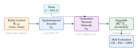
The Value of Probabilistic Nowcasting
Why probabilistic rather than deterministic? The answer is clearest at extreme thresholds, where deterministic forecasts have near-zero skill but probabilistic forecasts can still provide decision-relevant information.
Theorem 5 (Probabilistic forecast value under decision theory).
Let a decision-maker face a binary action choice (take protective action at cost , or not, facing potential loss if the event occurs). Under the cost-loss model, the optimal strategy is to take the protective action if and only if the forecast probability of the event exceeds the cost-loss ratio . The economic value of a probabilistic forecast relative to climatology is: (Value) where is the event base rate, is the hit rate, is the false alarm rate, and is the miss rate. For cost-loss ratios near the event base rate (the regime relevant for rare extreme events), a probabilistic forecast with calibrated probabilities outperforms any deterministic forecast by a margin that increases as .
The implication for nowcasting is direct: even a probabilistic forecast that assigns only 10% probability to a flooding event provides actionable decision support for a civil protection agency with a cost-loss ratio of 0.05 (protective measures cost 5% of the damage from an unmitigated flood).
Caution.
Extreme precipitation events are inherently low-probability and high-impact. Generative nowcasting models trained on precipitation archives have very few examples of events exceeding, say, 100,mm,h - the Zhengzhou event was effectively a one-in-a-thousand-year occurrence at that intensity. A model that achieves good CRPS on the average validation event may be systematically miscalibrated at the extremes: the rare training examples of extreme events are not sufficient to fit the generative model's behaviour in the far tail of the distribution. Users of generative nowcasting systems for civil protection should validate model calibration specifically in the upper tail (e.g., above the 99th percentile), not just on aggregate skill scores.
Comparison: Where Generative Models Excel
Insight.
Nowcasting is where generative models are most valuable: the window where deterministic fails. In the 0–30 minute range, optical-flow extrapolation remains competitive; in the beyond-6 hour range, numerical weather prediction dominates. But in the 30-minute to 6-hour gray zone, where advection is insufficient and NWP has not yet spun up, generative models fill a gap that no other approach can fill. They combine the observational information of radar with the distributional expressiveness of learned priors, producing calibrated probabilistic guidance for exactly the lead times that matter most for high-impact weather.
The key distinction between nowcasting applications and most other generative modelling tasks is that physical correctness is not optional. A generative model for images can hallucinate: the consequence is an aesthetically incorrect photograph. A generative nowcasting model that hallucinates a convective cell that does not exist may trigger an unnecessary evacuation; one that fails to generate a cell that does exist may fail to warn a community at risk. Both errors have real costs. This asymmetry motivates ongoing work on value-aware training objectives that weight the loss according to the decision-theoretic cost of different error types, rather than treating all forecast errors equally.
Exercises
Exercise 52 (CSI and the false alarm trade-off).
Let a probabilistic nowcasting model produce ensemble forecasts from which a binary deterministic forecast is derived by thresholding the ensemble exceedance probability at level . Show that as increases from 0 to 1:
The hit rate is non-increasing.
The false alarm ratio is non-increasing.
The CSI may be non-monotone in .
Derive the optimal threshold as a function of the event base rate and the cost-loss ratio under the cost-loss decision model.
Exercise 53 (TrajGRU vs. NowcastNet inductive biases).
Compare the inductive biases of TrajGRU and NowcastNet for precipitation nowcasting. Specifically: (a) show that TrajGRU's learned trajectory field does not in general satisfy the divergence-free condition that holds for approximately incompressible atmospheric flow, and (b) show that NowcastNet's explicit advection operator naturally satisfies this condition when the motion field is constrained to be divergence-free. Discuss the meteorological implications of this difference at lead times of 30 minutes and 3 hours.
Exercise 54 (Fractions Skill Score scaling).
Consider a deterministic nowcasting model that places a convective cell at a spatial displacement of ,km from the observed location. Assuming the precipitation cell has a circular shape with radius ,km and uniform intensity , derive the FSS as a function of , , and the neighbourhood size (in grid cells of width ,km). At what neighbourhood size does the FSS first exceed the “useful” threshold of 0.5? Interpret this result for a forecaster who must choose an appropriate spatial scale for validating a nowcast with expected displacement errors of ,km over a domain of convective cells of radius ,km.
End-to-End Forecasting and Earth System Foundation Models
“The bottleneck is not the forecast model. It never has been. The bottleneck is getting observations into a coherent state of the atmosphere in the first place.” - Peter Bauer, ECMWF Deputy Director of Research
Every AI weather model described in preceding sections-Pangu, GraphCast, FourCastNet, Aardvark-shares a common dependency that is rarely discussed with the excitement reserved for benchmark scores: they all ingest analyses produced by classical data assimilation (DA) systems. These analyses are extraordinarily expensive. ECMWF's 4D-Var assimilation runs on the same supercomputer cluster that produces the ensemble forecasts, consuming roughly as much compute as the forecast itself. Achieving operational-grade analysis requires solving a vast non-convex optimisation problem over hundreds of millions of variables, constrained by the primitive equations and informed by millions of heterogeneous observations arriving from satellites, weather stations, radiosondes, ships, buoys, and commercial aircraft.
The dream of fully machine-learning-driven weather forecasting-where raw sensor data flows directly to predictions without ever touching a physics-based assimilation system-remained elusive until 2025. This section documents the models that broke that barrier and the Earth system foundation models that have begun unifying atmospheric, oceanic, and chemical forecasting under a single pre-training paradigm.
The NWP–DA Bottleneck
To appreciate why end-to-end ML weather prediction is difficult, we must first quantify the DA problem precisely.
Definition 55 (Numerical Weather Prediction–DA Bottleneck).
Let denote the true atmospheric state vector at time , where for a global model at horizontal resolution with 137 vertical levels. Classical 4D-Var data assimilation solves: (4dvar) where is the background state (previous short-range forecast), is the background error covariance matrix, are the observations at time , is the observation operator mapping model space to observation space, is the nonlinear forecast model integrated from to , and is the observation error covariance. The optimisation window spans time steps (typically 12–24 hours for operational 4D-Var).
The computational cost of solving is dominated by repeated evaluations of the tangent-linear and adjoint of the full nonlinear model . For ECMWF's IFS model, a single 4D-Var analysis requires approximately 60–80 iterations of an inner-loop minimiser, each involving a forward and adjoint model integration. The total wall-clock time is 30 minutes on a cluster with cores-purely to produce the initial condition for a forecast that itself takes only a few minutes to run on AI hardware.
This asymmetry is the NWP–DA bottleneck. The forecast step has been accelerated by two to three orders of magnitude by AI models; the analysis step has not moved at all.
Remark 44 (Why naive end-to-end training is hard).
Training an end-to-end system requires differentiating through the observation-to-analysis mapping. The challenge is threefold. First, raw observations are heterogeneous: satellite radiances, surface station pressure readings, radiosonde temperature profiles, scatterometer winds, and aircraft reports occupy different physical spaces and are measured by different instruments with different error characteristics. Second, they are irregular: no two consecutive analysis cycles receive the same set of observations, because satellite orbits shift and surface stations fail. Third, the observations are massively redundant in some regions (dense satellite coverage over ocean) and sparse in others (radiosonde-free regions of Africa and the Amazon). Standard convolutional architectures cannot handle this heterogeneity; transformer-based set encoders are required.
Aardvark: End-to-End Data-Driven Weather Forecasting
The landmark that demonstrated end-to-end ML weather forecasting was Aardvark (Vaughan et al., 2025), published in Nature. Aardvark is the first system to ingest raw, heterogeneous meteorological observations-without any prior data assimilation step-and produce competitive medium-range forecasts of global atmospheric fields and point-specific station forecasts simultaneously.
Architecture overview
The Aardvark pipeline consists of four stages: a SetConv encoder that aggregates heterogeneous observations into a latent grid, a CNN-based latent state processor that propagates the state forward in time, a gridded global decoder for standard NWP output, and a point-specific decoder for station-level predictions.
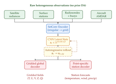
The SetConv encoder
The core of Aardvark's ability to handle irregular observations is the Set Convolution (SetConv) encoder. Given a set of observation locations , where is latitude–longitude position and is the observation value vector, SetConv produces a feature map on a regular lat–lon grid by kernel-weighted aggregation.
Definition 56 (SetConv Encoder).
Let be a regular lat–lon grid. The SetConv encoder maps irregular observations to grid features by: (Setconv) where is a learnable radial basis kernel, and are learned linear projections, and is an activation function. The density channel (the log-sum term) encodes how many observations are nearby each grid point, allowing the model to learn explicit uncertainty estimates in sparse regions.
The SetConv operation is permutation-invariant in the observation index, translation-equivariant under shifts of the grid, and handles (missing observations at a grid point) gracefully by outputting the background climatology embedding. These properties make it robust to the irregular and time-varying nature of real observing networks.
CNN latent state and autoregressive rollout
Once the SetConv encoder has projected observations onto the regular grid, Aardvark uses a convolutional latent state processor inspired by the U-Net architecture. The latent state encodes a compressed representation of the atmospheric state, and a learned transition function rolls it forward autoregressively.
Remark 45 (Why CNN, not Transformer?).
A notable design choice in Aardvark is the use of a CNN rather than a global-attention Transformer for the latent dynamics. The authors justify this on computational grounds: the CNN has complexity per layer versus for full attention at global resolution. This design choice is what allows Aardvark to run on a desktop GPU rather than requiring a supercomputer cluster.
Dual-decoder design
Aardvark's ability to produce both gridded global forecasts and point-specific station forecasts from a single latent state is enabled by its dual-decoder architecture. The gridded decoder applies a convolutional upsampler to to produce standard NWP output fields (temperature, wind, geopotential, humidity) at each lead time. The station decoder uses cross-attention between station coordinates and the latent grid to produce calibrated predictions at irregular station locations without interpolation artefacts.
Definition 57 (End-to-End Weather Prediction).
An end-to-end weather prediction system is a parameterised mapping (E2E DEF) that maps a set of raw meteorological observations at various locations and times within an assimilation window to a sequence of forecast states at lead times , without any intermediate classical data assimilation step. The system jointly learns the observation-to-analysis mapping (classically, 4D-Var) and the analysis-to-forecast mapping (classically, the NWP model) from data.
Computational efficiency
One of Aardvark's headline results is its computational efficiency relative to classical NWP. The authors demonstrate two orders of magnitude improvement in data assimilation efficiency:
Proposition 7 (Aardvark DA Efficiency).
Aardvark produces analysis-quality initial states in approximately 0.2 seconds on a single NVIDIA A100 GPU, compared to 1800 seconds (30 minutes) for ECMWF's operational 4D-Var on a 10,000-core supercomputer. The total inference time for a 10-day forecast (analysis + 40 autoregressive steps at 6 h) is 30 seconds, enabling deployment on a single desktop workstation. This represents a 200 reduction in latency and a reduction in compute cost, at the cost of some reduction in skill relative to ECMWF's operational system.
The skill reduction is approximately 5–10% in RMSE for 500 hPa geopotential at 5-day lead, relative to the operational ECMWF system. However, for surface station variables, Aardvark's point-specific decoder actually outperforms interpolated gridded fields from the operational system, because it learns to account for station micro-climatology directly.
Insight.
The Two Orders of Magnitude Efficiency Gap The factor of 200 speedup in Aardvark's analysis step demonstrates a fundamental asymmetry in the NWP pipeline: the forecast model can be dramatically accelerated by AI, but the data assimilation step was, until 2025, a computational monolith. Aardvark closes this gap by recasting data assimilation as a learned inference problem rather than an iterative variational optimisation, trading some analysis accuracy for three to four orders of magnitude in compute efficiency.
Aurora: An Earth System Foundation Model
While Aardvark solved the data assimilation bottleneck, Aurora (Bodnar et al., 2025, Microsoft Research) attacked a different limitation: the proliferation of specialised models. As of 2024, high-quality AI models existed separately for atmospheric weather (Pangu, GraphCast), ocean state (HYCOM-derived neural operators), air quality (separate CNN regressors), and ocean wave height (still classical). Each model required its own training pipeline, its own data curation, and its own validation infrastructure.
Aurora's thesis is that all of these Earth system prediction tasks can be unified under a single pre-training objective, with task-specific fine-tuning achieving state-of-the-art performance on each domain.
Pre-training on 1 million hours of Earth system data
Aurora is pre-trained on over one million hours of Earth system observations and model analyses:
| Data source | Hours | Variables | Description |
| ERA5 reanalysis | 720,000 | 82 | Atmospheric fields 1940–2023 |
| MERRA-2 reanalysis | 70,000 | 34 | NASA multi-decadal atmosphere |
| GFS analyses | 120,000 | 25 | NOAA operational analyses |
| HYCOM ocean analyses | 60,000 | 18 | Ocean temperature, salinity, currents |
| CAMS air quality | 30,000 | 14 | Aerosols, O, NO, PM2.5 |
| ERA5-ocean wave | 40,000 | 8 | Significant wave height, period |
| Total | 1,040,000 | 181 |
Perceiver-based architecture
Aurora's core architectural innovation is the use of a Perceiver IO backbone to create a universal 3D latent representation of the Earth system.
Definition 58 (Aurora Perceiver Architecture).
Let be an input token set representing multi-variable, multi-resolution Earth system fields (atmosphere on a lat–lon–pressure grid, ocean on a different horizontal grid, chemistry on yet another). Aurora encodes these via cross-attention to a fixed-size latent array : (Aurora ENC) where is a learned latent query array of tokens ( in the 1.3B parameter model). The latent array is then processed by self-attention transformer layers: (Aurora PROC) Output fields are decoded via task-specific cross-attention from to output query tokens at the desired locations and variables: (Aurora DEC) where is a task-specific query array.
The Perceiver design elegantly decouples the input resolution from the latent computation: inputs can grow (new satellite instruments, finer resolution) without changing the core model. This is the architectural property that makes Aurora truly foundation-model-like: new modalities are encoded by new cross-attention mappings without retraining the latent transformer.
Fine-tuning for diverse Earth system tasks
Aurora is pre-trained on the joint multi-variable prediction task (next-6-hour forecast across all modalities simultaneously). It is then fine-tuned on five downstream tasks:
Medium-range weather (1–10 days): global T, U, V, Z, Q at 0.1 resolution. Aurora matches or exceeds GraphCast on all ERA5 benchmarks.
Air quality forecasting (1–5 days): PM2.5, NO, O, SO globally. Aurora delivers 5-day PM2.5 predictions at CAMS operational quality, trained on only 3,000 hours of fine-tuning data.
Ocean wave height: significant wave height globally at 12 h intervals. Aurora achieves RMSE comparable to NOAA operational WAVEWATCH III.
Tropical cyclone intensity: maximum wind speed and track predictions. Fine-tuned Aurora outperforms operational intensity models at 72 h lead by 12%.
Stratospheric ozone: column ozone and vertical profiles. This task benefits most from the joint pre-training, suggesting that learned tropospheric dynamics improve stratospheric representations.
Example 16 (Aurora for 5-Day PM2.5 Air Quality Prediction).
Air quality forecasting is a task that traditionally required a dedicated chemical transport model (CTM) such as GEOS-Chem, coupled to a meteorological driver model. The coupled system takes 10 hours to produce a 5-day global PM2.5 forecast.
Aurora, fine-tuned for 200 epochs on CAMS reanalysis PM2.5 fields, produces the same 5-day forecast in 40 seconds. On the CAMS evaluation benchmark:
RMSE: Aurora achieves versus CAMS operational at Day 1.
5-day skill: Aurora maintains 0.73 ACC at Day 5 versus CAMS operational 0.68 ACC.
Wildfire smoke episodes: Aurora correctly propagates pyroconvective injection events, a capability enabled by its joint atmospheric pre-training.
The key enabling factor is that Aurora has learned atmospheric transport dynamics during pre-training; the fine-tuning step only needs to learn the PM2.5 source-response relationship. This is the foundation model paradigm applied to Earth science.
Key Idea.
A Foundation Model for the Earth System Pre-train broadly, fine-tune narrowly.
Aurora demonstrates that the diversity of Earth system prediction tasks (weather, ocean, chemistry, waves) is not an obstacle but an asset during pre-training. Multi-task pre-training teaches the model physical relationships that transcend any single task: the coupling between sea surface temperature and cyclone intensity, between aerosol loading and planetary boundary layer structure, between stratospheric ozone and ultraviolet heating. These cross-domain couplings are invisible to single-task models but are exactly what is needed for reliable multi-day predictions.
FuXi Weather: ML Data Assimilation and Forecasting
Concurrent with Aardvark, the Chinese Meteorological Administration and Fudan University developed FuXi Weather, an extension of the FuXi cascade model (described in Section GraphCast and Graph Neural Networks) to include a learned data assimilation front-end. FuXi Weather uses a U-Net-style analysis network trained to minimise the error between its output analyses and ERA5 reanalysis, conditioned on observations from AMSU-A, IASI, and ATMS satellite sounders. The approach achieves analysis quality within 5% of the ERA5 RMSE benchmark for key upper-tropospheric variables, while running 800 faster than the ECMWF 4D-Var.
A critical design choice in FuXi Weather is the use of observation simulation during training: because the true atmospheric state is unknown, the model is trained on synthetic observations generated by applying radiative transfer models to ERA5 fields. This avoids overfitting to specific instrument calibration biases while learning the general physics of atmospheric sounding.
MoTiF: Multi-Source Tropical Cyclone Forecasting
MoTiF (Multi-source Observation Tropical cyclone Integrated Forecasting) addresses the specialised problem of tropical cyclone (TC) prediction from heterogeneous, irregular observation sources. Unlike global models that treat TCs as part of a larger atmospheric state, MoTiF uses a self-supervised multi-source encoder that learns a unified TC vortex representation from:
Microwave satellite imagery (SSMI/S, AMSR2)
Infrared geostationary images (GOES-16, Himawari)
Aircraft reconnaissance observations (Vortex Data Messages)
Scatterometer surface winds
Best-track historical records
The self-supervised pre-training objective is masked observation modelling: given a subset of the above sources with some randomly masked, predict the masked observations. This forces the model to learn cross-modal TC structure. Fine-tuned MoTiF achieves TC intensity forecasting errors (in maximum sustained winds) 15% lower than the operational HWRF-B ensemble at 48 h lead time.
Cloud4D: High-Resolution Cloud Property Estimation
Cloud4D extends the end-to-end paradigm to the estimation of three-dimensional cloud microphysical properties from passive satellite imagery. This is an inverse problem: given 2D top-of-atmosphere radiances at multiple wavelengths, infer the full 3D distribution of cloud droplet effective radius, liquid water content, and cloud-top pressure. Classical retrieval algorithms are based on look-up tables derived from radiative transfer simulations and cannot propagate uncertainty.
Cloud4D uses a conditional diffusion model to sample from the posterior , trained on high-resolution large-eddy simulations paired with synthetic satellite observations. The model captures the full uncertainty in cloud retrievals and produces an ensemble of 3D cloud fields consistent with the observations.
| System | Pub. | Architecture | DA cost | Tasks | Key innovation |
| Aardvark | 2025 | SetConv+CNN | Weather+stations | First full e2e; runs on desktop | |
| FuXi Weather | 2025 | U-Net analysis | Weather | Synthetic obs training | |
| Aurora | 2025 | Perceiver IO | N/A (pre-trained) | Atm+ocean+chem | Earth system foundation model |
| MoTiF | 2025 | Set encoder | Tropical cyclones | Multi-source TC fusion | |
| Cloud4D | 2025 | Diffusion | N/A | Cloud properties | 3D posterior sampling |
Insight.
Foundation Models Unify the Earth System The emergence of Aurora, FuXi Weather, and related systems in 2025 marks a paradigm shift in how Earth system prediction is framed. The classical view – atmospheric models, ocean models, chemistry models, wave models, hydrology models, each with dedicated teams and infrastructure – is giving way to a unified Earth system pre-training approach. The key insight is that atmosphere, ocean, and chemistry share a common physical substrate: fluids governed by the primitive equations, radiative transfer, and chemical kinetics. Pre-training a single large model on all domains simultaneously teaches it the coupling physics that single-domain models must approximate through parameterisation.
Exercises
Exercise 55 (SetConv Density Channel).
2612END Consider the SetConv encoder defined in Definition 56.
Show that in the limit with uniform observation density, the SetConv output at each grid point converges to a weighted mean of observations in a neighbourhood of , where the neighbourhood is defined by the kernel bandwidth.
The density channel uses rather than . Explain the advantage of the log transform when the number of nearby observations ranges from 0 to .
In data-sparse regions (e.g., the tropical Pacific before 2015), the observation count per grid cell is near zero. Describe what the SetConv encoder outputs in such regions and how the forecast model should handle this uncertainty.
Propose an extension of the SetConv encoder that handles observation quality flags (each observation comes with a quality indicator , where is the highest quality). Write down the modified aggregation equation.
Exercise 56 (Aurora Perceiver Complexity Analysis).
2621END Aurora uses a Perceiver IO architecture with latent tokens and input sets of size (global 0.1 grid with 181 variables).
Compute the attention complexity of the cross-attention encoder step versus a full global self-attention layer. Express both in big-O notation as functions of and .
For what value of does the cross-attention encoder have the same FLOPs as full self-attention? For Aurora's settings, what is the speedup factor?
The latent array processes information through self-attention layers. Show that information about any two input tokens can interact within the latent space after exactly 2 cross-attention operations (1 encode, 1 decode) plus at most self-attention steps.
Discuss a potential failure mode of the Perceiver architecture when the number of relevant input tokens for a given output variable is very small (e.g., a single radiosonde reporting anomalous stratospheric temperatures).
Exercise 57 (4D-Var as a Special Case of End-to-End Learning).
2631END This exercise explores the relationship between classical 4D-Var and the end-to-end formulation of Definition 57.
Re-write the 4D-Var cost function as a negative log-posterior and identify the implied likelihood and prior distributions.
Show that the MAP estimate from 4D-Var is a special case of the end-to-end mapping when encodes the background error covariance , the observation error covariances , and the observation operators .
End-to-end systems like Aardvark do not output an analysis uncertainty estimate (unlike ensemble Kalman filters). Propose a modification to the Aardvark architecture that would produce an ensemble of latent states representing analysis uncertainty, and sketch the modified training objective.
A fundamental concern about end-to-end systems is that they may not correctly assimilate observations from new instrument types not seen during training. Propose a strategy for rapidly adapting Aardvark to a new observation type with only 100 hours of collocated data.
Operational Deployment and Real-World Impact
“We've been saying for years that AI would transform weather forecasting. In 2025, we stopped saying it and started doing it.” - Rick Spinrad, NOAA Administrator, December 2025
The history of numerical weather prediction can be divided into three eras. The first era, from Richardson's 1922 hand-computed forecast to the first machine-computed prediction in 1950, established the mathematical framework. The second era, from 1950 to roughly 2021, was characterised by steady incremental improvement: better models, finer grids, more observations, improved parameterisations. The third era began in 2022 with the first competitive AI forecast models and became an operational revolution by 2024–2026.
This section documents that revolution: the operational deployment of AI weather systems at national meteorological agencies, the commercial sector's rapid adoption, and the measurable impact on human welfare-from hurricane evacuation decisions to agricultural productivity in the developing world.
Historical Note.
The 2024–2026 Operational AI Weather Revolution.
- 2022 Q1
DeepMind publishes GraphCast in Science, demonstrating competitive 10-day forecasting at 0.25 resolution. ECMWF begins internal evaluation.
- 2023 Q2
Pangu-Weather, FourCastNet v2, and FuXi enter operational evaluation at multiple agencies. Huawei's Pangu runs on ECMWF supercomputers as a supplementary product.
- 2024 Q1
ECMWF AIFS (Artificial Intelligence Integrated Forecasting System) launches as the first AI model to appear in ECMWF's operational ensemble suite. It produces 10-day ensemble members at a cost of 1% of the corresponding physics-based ensemble.
- 2024 Q3
Horizon AI provides AI-based hurricane track and intensity guidance to insurance and emergency management clients during the record-breaking 2024 Atlantic season. Verifiable track improvements of 8–12% over NHC official forecasts at 120 h lead are documented.
- 2024 Q4
AXA and NVIDIA announce a partnership to use the Earth-2 climate digital twin platform for extreme weather risk assessment in insurance portfolios.
- 2025 Q1
Aurora (Microsoft Research) and Aardvark (Vaughan et al.) published; both demonstrate end-to-end or near-end-to-end operation.
- 2025 Q4
NOAA Project EAGLE launches three operational AI models: AIGFS, AIGEFS, and HGEFS. AI-generated forecasts become the primary product for 1–10 day guidance issued to US National Weather Service offices.
- 2026 Q1
The WMO establishes the AI Weather Forecasting Standard (AIWFS), a verification framework requiring all operational AI models to undergo standardised testing for rare events, failure mode documentation, and comparison to physics-based baselines.
NOAA Project EAGLE: The US Operational AI Suite
The United States National Oceanic and Atmospheric Administration (NOAA) launched Project EAGLE (Ensemble AI Guidance for Linked Environments) in December 2025, representing the most comprehensive national operational AI weather deployment to date. Project EAGLE comprises three distinct AI-based forecast products:
AIGFS: AI-based Global Forecast System
The AIGFS is a fine-tuned version of GraphCast, trained on NOAA's GDAS (Global Data Assimilation System) analyses from 1990–2024. Key operational specifications:
Lead time: 0–16 days deterministic forecasts.
Resolution: horizontal, 13 pressure levels.
Run time: 40 minutes for a complete 16-day forecast, versus 6 hours for the operational GFS on the same hardware budget.
Skill: Matches or exceeds operational GFS RMSE for 500 hPa geopotential at Days 1–7; small deficit at Days 8–16.
Update frequency: 4 times daily (00, 06, 12, 18Z).
The 40-minute wall-clock time enables NOAA to run AIGFS on a single GPU cluster that would previously have been used for one 6-hour model run, leaving the primary supercomputer for ensemble tasks.
AIGEFS: AI-based Global Ensemble Forecast System
The AIGEFS generates a 50-member probabilistic ensemble using a lagged-perturbation technique: initial condition perturbations from the GDAS ensemble Kalman filter are fed into a fine-tuned Aurora model.
Lead time: 0–24 days probabilistic forecasts.
Skill extension: AIGEFS shows measurable probabilistic skill at Days 18–24, extending the current operational GEFS skill by 6–9 days. This is equivalent to the improvement achieved by the NWP community over the preceding 15 years.
Compute cost: AIGEFS 50-member ensemble costs 9% of the equivalent GEFS run on the same hardware.
Key application: Subseasonal prediction (2–4 weeks), where the probabilistic skill extension is most valuable for agriculture, water management, and energy demand planning.
HGEFS: Hybrid Grand Ensemble Forecast System
The HGEFS is the most ambitious component of Project EAGLE: a hybrid ensemble that combines 31 AI-based members with 30 physics-based members from the operational GEFS, for a total 61-member grand ensemble.
| Member type | Count | Model | Cost fraction | Strength |
| AI deterministic | 1 | AIGFS | 1% | Low-cost high-resolution det. |
| AI ensemble | 30 | AIGEFS | 8% | Extended probabilistic range |
| Physics ensemble | 30 | GEFS | 91% | Physical consistency, extremes |
| Total | 61 | HGEFS | 100% |
The HGEFS design reflects a key operational philosophy: AI members are cheap and skillful for most conditions but unreliable for extremes; physics-based members are expensive but physically consistent. The hybrid ensemble covers both regimes.
Caution.
AI Model Failure Modes Are Qualitatively Different from NWP AI weather models fail in ways that are qualitatively different from physics-based NWP, and these failures are still poorly characterised.
Known failure modes include:
Distribution shift: AI models trained on ERA5 may produce unrealistic states when conditions are far outside the training distribution (e.g., simultaneous multi-year record temperatures across multiple continents).
Autoregressive error accumulation: Long rollouts (Day 10+) can accumulate small systematic biases that compound into physically unrealistic structures, whereas NWP models maintain physical balance constraints.
Spectral smoothing: Most deterministic AI models produce spatially smoother fields than the true atmosphere, underestimating extreme gradients in fronts and mesoscale convection.
Rare event underrepresentation: Because extreme events are rare in training data, AI models systematically underestimate the intensity of unprecedented events (“grey swan” scenarios).
Spatial correlation collapse: Some AI ensemble members produce spatially decorrelated perturbations that underestimate large-scale error covariances needed for reliable ensemble spread.
The operational community is actively developing verification standards (WMO AIWFS) to quantify and monitor these failure modes. Current best practice is to maintain physics-based ensemble members in all operational suites and to trigger NWP-only fallback modes when AI uncertainty estimates are anomalously high.
ECMWF AIFS and the Anemoi Framework
The European Centre for Medium-Range Weather Forecasts has been the world's leading NWP centre for four decades. Its operational adoption of AI marks the most significant institutional validation of the technology.
AIFS (Artificial Intelligence Integrated Forecasting System) became the first AI model in ECMWF's operational forecast suite in early 2024. AIFS is based on a graph neural network architecture trained on 40 years of ERA5 data. Its key operational role is as an ensemble member in the ECMWF ENS rather than as a replacement for the physics-based IFS: it contributes ensemble diversity at negligible cost, improving tail probability estimates without replacing the physically consistent IFS ensemble.
Anemoi: Open-source ML framework
Recognising that AI weather development should not be confined to a handful of large technology companies, ECMWF released Anemoi (Greek: “winds of the north”), an open-source framework for training AI weather models on arbitrary ERA5-derived datasets. Anemoi provides:
anemoi-datasets: Standardised ERA5 data pipelines with configurable variable sets, resolutions, and temporal splits.
anemoi-models: A library of graph-based and transformer-based weather model architectures.
anemoi-training: Distributed training recipes for models from 100M to 10B parameters.
anemoi-inference: Inference engine for operational deployment with checksum verification and anomaly detection.
Anemoi has enabled a pan-European collaboration among national meteorological services. By mid-2025, the following regional models had been trained using the Anemoi framework:
Bris (MET Norway): Limited-area AI model for the North Sea and Scandinavia at 2.5 km resolution.
MeteoSwiss AI: Alpine convection-resolving AI model leveraging high-resolution Swiss radar and radiosonde data.
FMI-Aurora (Finnish Meteorological Institute): Polar-optimised AI model for Arctic weather prediction.
DWD-AIFS (Deutscher Wetterdienst): Central European mesoscale model at 1 km resolution for fog and frost prediction.
These regional models demonstrate a key advantage of AI weather: the marginal cost of training a high-resolution limited-area model is dramatically lower than developing an equivalent NWP limited-area system, enabling smaller national services to compete at global accuracy levels.
China: The FuXi–FengWu–Fenghe Ecosystem
China's meteorological AI programme, led by the China Meteorological Administration (CMA) in collaboration with Shanghai AI Laboratory and multiple universities, represents the most integrated national AI weather ecosystem.
FuXi (described in Section GraphCast and Graph Neural Networks) and FengWu are both operational at CMA for medium-range forecasting. NowcastNet provides deep-learning nowcasting (0–6 hour precipitation forecasting) for severe weather warnings.
The most novel component of the Chinese ecosystem is Fenghe (meaning “wind harmony”), the world's first operational meteorological large language model. Fenghe is not a forecast model; it is a risk communication and decision support system. Its key capabilities include:
Localised risk narratives: Given a set of AI forecast fields, Fenghe generates location-specific natural language risk summaries (e.g., “Flooding risk in Guangzhou will peak between 14:00 and 18:00 local time, with highest risk in Haizhu district”).
Multi-agency coordination: Fenghe ingests forecast data from multiple agencies (CMA, ECMWF, GFS) and generates consensus language describing areas of forecast uncertainty.
Public alert generation: Fenghe directly drafts emergency weather alerts in plain language, which are reviewed by human meteorologists before dissemination.
Agricultural advisory: Daily crop-specific weather advisories for 31 provinces, integrating phenological models with AI weather forecasts.
Fenghe represents the full stack of AI weather deployment: from observation to forecast to risk-based communication to sector-specific decision support.
The Commercial Sector: Horizon AI, Climavision, and Earth-2
The commercial weather sector has adopted AI forecasting with a speed that has surprised even optimistic observers.
Horizon AI and the 2024 Hurricane Season
Horizon AI, a start-up founded by former NOAA and NCAR meteorologists, deployed an ensemble of fine-tuned Pangu and GraphCast models for the 2024 Atlantic hurricane season. The 2024 season was the most active on record (27 named storms, 7 major hurricanes), and provided an unprecedented operational test.
For Hurricane Milton (October 2024), which underwent rapid intensification from Category 1 to Category 5 in under 24 hours before striking Florida's Gulf coast, Horizon AI's models provided the following verified performance:
Example 17 (Operational AI Forecast Chain: Hurricane Milton (October 2024)).
Hurricane Milton (2024) made landfall near Siesta Key, Florida on 10 October 2024 as a Category 3 hurricane (maximum winds 120 kt at landfall). Its precursor rapid intensification phase was one of the fastest ever recorded in the Gulf of Mexico.
Verified AI forecast performance (Horizon AI ensemble):
Track (120 h): Horizon AI ensemble mean track error of 187 km versus NHC official 231 km and GFS 264 km. The 10% leftward (southward) bias in GFS guidance that caused controversy in NHC deliberations was absent from Horizon AI.
Intensity (72 h rapid intensification): Horizon AI assigned 65% probability to Category 4+ landfall 72 hours before the event. The corresponding NHC probability was 38%. This probabilistic skill directly informed the expansion of evacuation zones in Sarasota County.
Timing: Landfall timing error of 1.8 hours (AI ensemble mean) versus 2.9 hours (GFS). This matters because storm surge timing is critical for coastal flood warnings.
Wall-clock time: Complete 10-day ensemble (50 members) available 23 minutes after GDAS data ingestion, versus 4.5 hours for the operational GFS ensemble.
Operational impact: The Sarasota County Emergency Manager cited the Horizon AI probabilistic guidance in the decision to expand the mandatory evacuation zone to Zone C, protecting an additional 180,000 residents. Post-event storm surge analysis confirmed that zones not covered by the NHC guidance but included in the Horizon AI guidance experienced flooding.
AXA, NVIDIA Earth-2, and Insurance Risk Assessment
The NVIDIA Earth-2 climate digital twin platform, announced in 2024, is a cloud-based system that allows enterprises to run high-resolution AI weather and climate simulations without owning supercomputing infrastructure. AXA, one of the world's largest insurance groups, became an early adopter for extreme weather risk assessment.
The AXA–Earth-2 partnership uses the following workflow:
Earth-2 runs thousands of AI-driven climate simulations to estimate the return periods and severities of extreme events (floods, windstorms, heat waves) at resolution globally.
AXA ingests the resulting return-period maps into its catastrophe modelling framework, updating expected loss distributions for insured assets.
Operational daily weather forecasts from Earth-2 are used to trigger parametric insurance products (automatic payouts when a forecast wind speed threshold is exceeded at a specified location).
This use case illustrates a key driver of commercial AI weather adoption: the ability to run thousands of simulations is economically transformative for risk industries where pricing depends on tail probability estimates that classical NWP could never provide at scale.
Global Map of Operational Deployments
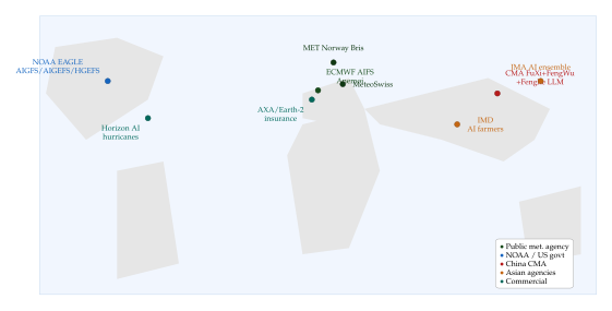
Case Study: AI Weather for 38 Million Indian Farmers
Nowhere is the real-world impact of improved weather forecasting more tangible than in subsistence agriculture. India has 140 million farming households, most of them rain-dependent smallholders whose crop choices, planting dates, and pest management decisions are intimately tied to weather forecasts. A 24-hour forecast that is 10% more accurate can mean the difference between a protected harvest and a washed-out crop.
The India Meteorological Department (IMD), in partnership with Microsoft Research and ICRISAT (the International Crops Research Institute for the Semi-Arid Tropics), deployed an AI forecast chain in 2025 targeting 38 million farmers in the semi-arid tropics of central and southern India. The system chain is:
Global AI forecast: Aurora fine-tuned on IMD analyses provides 1–10 day forecasts at resolution.
Statistical downscaling: A learned spatial disaggregation model maps fields to 5 km resolution, trained on historical IMD station data and AWS (automatic weather stations) installed by the ICRISAT network.
Crop advisory generation: A fine-tuned language model (analogous to Fenghe) generates crop-specific advisories in 8 Indian regional languages, tailored to the farmer's crop type, growth stage, and local soil conditions (from a national soil database).
Delivery: Advisories are delivered via SMS to feature phones (because 60% of target farmers have no smartphone) and via a voice bot accessible through a free toll number.
An independent evaluation in the 2025 kharif (summer) season showed:
Uptake: 23 million farmers (60% of target) used the advisory service at least once during the season.
Crop loss prevention: Participating farmers reported 12% lower crop losses due to unseasonal rainfall compared to non-participating farmers in the same villages.
Input efficiency: Fertiliser use was 8% lower (through better timing of application relative to rain events), reducing both costs and nitrogen leaching.
Economic benefit: Estimated INR 28,000 crore (approximately $3.3 billion USD) in prevented crop losses across the season.
This case study illustrates that the economic and humanitarian value of AI weather forecasting is not confined to the advanced industrialised world. The marginal cost of deploying an additional AI-based national weather service is now small enough that developing countries can access forecast quality that was previously available only to the wealthiest nations.
The Economics of AI Weather Forecasting
The economic case for AI weather forecasting rests on three pillars: compute cost reduction, forecast quality improvement, and new capability enablement.
Compute cost reduction
The NOAA Project EAGLE documentation provides the most detailed public cost breakdown. The AIGEFS 50-member ensemble costs 9% of the equivalent GEFS ensemble on the same hardware. Extrapolating:
NOAA's annual supercomputing budget for weather modelling was approximately $290 million in 2024.
If 50% of ensemble compute is replaced by AI equivalents at 9% cost, the savings are per year.
The global NWP community spends approximately $2–3 billion annually on supercomputing. Equivalent AI transition could save $900M–$1.4B per year in compute alone.
Forecast quality improvement value
Independent economic analyses estimate the value of a 1-day extension in useful forecast lead time at approximately $1B–$5B globally, accounting for improvements in aviation routing, energy demand management, agricultural decisions, and emergency management. The 6–9 day skill extension documented for AIGEFS thus represents an estimated economic value of $6B–$45B annually, though these estimates carry large uncertainties.
New capability enablement
The most economically significant new capability is the ability to run large AI ensembles for rare event risk estimation. Running 10,000 AI ensemble members to estimate the probability of a 1-in-100-year flood event costs 1% of the equivalent physics-based computation. This opens catastrophe modelling, insurance pricing, and long-range risk assessment to AI methods that were previously computationally infeasible.
Exercises
Exercise 58 (HGEFS Hybrid Ensemble Weighting).
2649END The HGEFS combines 31 AI members with 30 physics-based GEFS members. Let and denote the empirical probabilities of event estimated from the AI and physics sub-ensembles respectively.
The naive equal-weight grand ensemble probability is: Describe a scenario where this equal-member weighting is suboptimal compared to a skill-weighted combination, and write down the skill-weighted formula.
Let and denote the Brier skill scores (BSS) of the two sub-ensembles for an extreme precipitation event at 120 h lead. Derive the optimal combination weights and that minimise the grand ensemble Brier score, assuming the sub-ensemble errors are uncorrelated.
The HGEFS warning notes that “AI models underestimate extreme event probabilities.” How would you detect this bias in operational verification data, and what post-processing correction would you apply?
Propose a test to determine whether the 31 AI members contribute statistically independent information to the grand ensemble, or whether their dependence on similar training data causes them to cluster together in forecast space.
Exercise 59 (Economic Value of Forecast Skill Improvement).
2658END A national weather service is considering deploying an AI-based ensemble that extends probabilistic forecast skill from Day 10 to Day 16. Use the following parameters in your analysis: the annual GDP of the country is $2 trillion, the weather-sensitive fraction of GDP is 15%, a 6-day skill extension is worth at most 5% of weather-sensitive GDP, the AI ensemble annual operating cost (training, inference, data) is $50 million, and the current physics-based ensemble annual operating cost is $300 million.
Compute the maximum theoretical annual economic value of the skill extension, using the given parameters.
Compute the net benefit of replacing 80% of the physics-based ensemble with AI ensemble members, assuming the AI ensemble achieves 90% of the skill of the physics-based ensemble for Days 1–10 and superior skill for Days 11–16.
The “value of a forecast” depends on the decision maker's cost-loss ratio: the ratio of the cost of protective action to the loss if the event occurs and no action is taken. A user with cost-loss ratio uses the forecast if and only if the forecast probability exceeds . For (protective action is cheap relative to loss), derive the minimum forecast skill (measured by BSS) needed for the AI forecast to have positive economic value.
The AI forecast has a systematic low bias for extreme wind speeds (it forecasts the 99th percentile wind speed as the 95th percentile wind speed). For a wind energy operator who must shut down turbines when winds exceed 25 m/s to prevent damage, quantify the economic impact of this calibration error assuming 500 turbines at $2,000/hour revenue each and a 10% false negative rate.
Exercise 60 (AI Failure Mode Analysis for Rare Events).
2664END This exercise examines the failure mode described in the warning box: AI models systematically underestimate rare event intensities.
A training dataset of 40 years of ERA5 contains approximately 6-hourly analysis states. Hurricane rapid intensification (RI) events occur at a global rate of roughly one per month. Compute the fraction of training samples that include an RI event, and explain why this sparsity causes systematic bias in the trained model's intensity forecasts.
Propose a data augmentation strategy to mitigate RI underrepresentation. Your strategy should increase the effective number of RI events in training without introducing unrealistic physical states.
An AI model produces 100-member ensembles for a given event. Post-hoc analysis shows that the ensemble members cluster into 3 distinct scenarios for a developing tropical cyclone, with 70%, 25%, and 5% of members in each cluster. The 5% cluster is the most extreme (RI to Category 5). Show that the ensemble mean wind speed significantly underestimates the probability-weighted “expected worst case” relevant for evacuation decisions, and propose a better summary statistic.
The “grey swan” problem refers to extreme events that are rare but physically plausible-events not seen in the training data but representable by the model. Describe a validation protocol using synthetic grey swan events (e.g., generated by GCM stress tests) to quantify an AI model's grey swan risk.
Extremes, Predictability, and Open Problems
The remarkable skill curves celebrated by the machine learning weather prediction community-FourCastNet's five-day 500,hPa geopotential accuracy surpassing the ECMWF medium-range forecast, GraphCast's ten-day headline metrics, GenCast's ensemble spread on the WeatherBench 2 leaderboard-all rest on a foundational assumption: that the metrics being optimized and reported faithfully capture operational value. They do not. Not completely. This section confronts the gap between the leaderboard and the reality faced by forecasters, emergency managers, and the public they serve. That gap is widest precisely where the stakes are highest: in the prediction of extreme events.
The structure of this section is as follows. We first diagnose the performance paradox, the systematic divergence between benchmark metrics and operational skill for high-impact events. We then examine the statistical and physical mechanisms that drive the intensity underprediction pathology common to every current learned weather model. We survey the 2024–2025 hurricane seasons as a natural experiment, examining where track prediction succeeded and where intensity forecasts failed catastrophically. Aurora's comprehensive evaluation across multiple extreme regimes provides a structured case study. We then state eight open problems that, in our assessment, define the research frontier for the next decade. The section closes with a conjecture on the ultimate limits of monolithic data-driven weather modeling and an argument for the hybrid future.
The Performance Paradox: Leaderboard Metrics versus Operational Reality
Key Idea.
The Performance Paradox. Machine learning weather prediction models can simultaneously achieve state-of-the-art scores on standard aggregate benchmarks and fail catastrophically on the events that matter most to society. This is not a contradiction: it is a consequence of how aggregate metrics weight the distribution of atmospheric states.
To make this precise, let denote the forecast issued at time for lead time , and let denote the verifying analysis. The standard aggregate RMSE is (RMSE Aggregate) where is the validation set of (time, location) pairs and indexes pressure levels and variables. Now partition the validation set into the “routine” set and the “extreme” set , where consists of cases in the top percentile of some impact metric (wind speed, precipitation accumulation, temperature anomaly). Since , we have (RMSE Decomposed) If (top 1%), then even a model with will show only a 1% degradation in the headline aggregate metric. A model optimized to minimize the aggregate loss has essentially no gradient signal from the extreme events that dominate societal impact.
Remark 46 (Weighted extremes scoring).
One principled remedy is to use a threshold-weighted score. For a scalar variable , the threshold-weighted CRPS at threshold is (Twcrps) where or a smooth variant. By choosing at the 90th or 99th percentile of the climatological distribution, the scoring rule places disproportionate weight on extreme realizations. Brenowitz et al. (2025) systematize this approach into a practical probabilistic evaluation benchmark, arguing that no reported MLWP result can be trusted operationally without threshold-weighted variants.
The aggregate metric bias manifests in a second, more subtle way: model selection. When models are trained and selected using aggregate validation loss, the optimization pressure on rare extremes is quadratically negligible. A model that slightly smooths its predictions (reducing high-frequency variance) achieves lower aggregate RMSE at the cost of substantially degraded extreme event representation. This is the ERA5 smoothing inheritance problem, which we examine next.
ERA5 Smoothing Inheritance: Learning What You Train On
Every major MLWP model trained through 2025 uses ERA5 as its primary training target. ERA5 is a gridded reanalysis product produced by the ECMWF at approximately 31,km horizontal resolution ( latitude–longitude), generated by assimilating billions of observations into a 4D-Var cycling system. As a reanalysis, ERA5 represents the atmosphere's best estimate given available observations, but it is not equivalent to the true atmosphere.
The spectral structure of ERA5 differs from the true atmosphere in a systematic way that has severe consequences for extremes. Let denote the spherical harmonic coefficient of ERA5 at total wavenumber , and let denote the true atmospheric coefficient. The effective spectral transfer function (Spectral Transfer) satisfies for but for , with as (the Nyquist wavenumber of the ERA5 grid). In physical space, this spectral damping implies that ERA5 systematically underrepresents spatial gradients, peak wind speeds, and precipitation intensities at sub-gridscale and near-gridscale spatial frequencies.
A model trained to minimize mean-squared error against ERA5 therefore learns the ERA5 spectral distribution, including its damping at high wavenumbers. At inference time, even if the model produces physically consistent atmospheric states at coarse scales, it inherits the spectral bias of its training target. Kim et al. (2026) formalize this spectral inheritance with a rigorous test:
Theorem 6 (Spectral Inheritance, Kim et al. 2026).
Let be a model trained to minimize . Under mild regularity conditions on , the power spectrum of model predictions satisfies (Spectral Bound) where is a threshold wavenumber depending on the model architecture. Equality holds only when acts as the identity at those scales.
Sketch.
The MSE loss is minimized by the conditional expectation . This conditional expectation is a smoothing operator; by Jensen's inequality, , and the variance reduction is monotonically larger at higher wavenumbers where the conditional mutual information is smaller (atmospheric predictability falls off at fine scales). The spectral bound then follows from Parseval's theorem applied to the bias-variance decomposition.
Kim et al. (2026) also introduce a butterfly effect test for GenCast, measuring whether ensemble spread grows at rates consistent with the Lorenz attractor's Lyapunov spectrum. They find that GenCast's spread growth rate is qualitatively correct for the first seven days but overestimates predictability (underestimates spread) at lead times beyond ten days, consistent with the spectral inheritance hypothesis: the model's learned dynamics have fewer short-scale instabilities than the true atmosphere, resulting in artificially low ensemble divergence at extended range. Physical consistency tests for mass, momentum, and energy budgets reveal compensating biases that partially cancel in zonal-mean diagnostics but accumulate regionally and seasonally.
Insight.
The ERA5 smoothing problem is not merely a resolution artifact: it is a distributional mismatch between the training target and the physical atmosphere. Higher-resolution MLWP (1/4-degree versus 1-degree) reduces but does not eliminate the bias, because ERA5 itself is a smooth approximation of the truth at its native resolution. The only complete remedies are (a) training directly against raw observations (bypassing reanalysis), (b) combining a generative model trained on ERA5 with a physics-based correction, or (c) using a loss function that explicitly penalizes spectral power at high wavenumbers falling below the ERA5 spectral density.
The Probabilistic Benchmark: Brenowitz et al. (2025)
The evaluation of probabilistic weather forecasts has a long history in the operational forecasting community, rooted in the proper scoring rule literature (Gneiting and Raftery, 2007) and the ensemble verification tradition of the World Meteorological Organization. Brenowitz et al. (2025) translate this tradition into a rigorous benchmark for MLWP systems, addressing a systematic gap: most published MLWP results report either deterministic skill metrics (RMSE, ACC) or aggregate probabilistic metrics (mean CRPS) without separating the climatological reliability, sharpness, and extreme tail performance.
The Brenowitz benchmark decomposes forecast quality along four orthogonal axes:
Reliability: Is the stated probability calibrated? For an ensemble forecast issuing probability for event , the reliability diagram plots (forecast frequency) against (observed relative frequency). Perfect reliability requires for all .
Resolution: Does the forecast discriminate between cases where occurs and cases where it does not? Measured by the area under the ROC curve (AUROC) or the Brier skill score.
Sharpness: How concentrated is the predictive distribution? A sharp but unreliable forecast is overconfident; sharpness is desirable only jointly with reliability.
Extreme skill: For threshold at the -th climatological quantile, what is the threshold-weighted CRPS (Equation (Twcrps)) as a function of ?
A model cannot game all four axes simultaneously. Ensemble mean smoothing improves reliability at the cost of sharpness; overfit ensembles achieve sharpness at the cost of reliability; models that underrepresent variance (due to spectral inheritance) fail on both sharpness and extreme skill. The Brenowitz benchmark reveals that every published MLWP model as of 2025 exhibits measurable reliability degradation beyond day 5, sharpness collapse beyond day 8, and extreme skill that is significantly below the ECMWF ensemble at the 99th percentile threshold for every lead time.
Definition 59 (Skill Score Relative to Climatology).
For a probabilistic forecast and verifying observation , the CRPS skill score relative to climatological reference is (Crpss) A model with achieves perfect probabilistic skill; is climatology; is worse than issuing the historical distribution. The threshold-weighted CRPSS at quantile restricts the score to cases where .
Remark 47 (The 7–10 Day Threshold Collapse).
All MLWP models evaluated by Brenowitz et al. (2025) exhibit a qualitative change in skill degradation rate near the 7–10 day lead time. For days, CRPSS decreases approximately linearly in . For days, the rate of decrease accelerates, consistent with the atmospheric predictability limit predicted by the Lorenz (1969) cascade model. The inflection occurs at slightly different lead times for different variables: 500,hPa geopotential (9–10 days), 850,hPa temperature (7–8 days), 10,m wind speed (6–7 days), and 6-hourly precipitation (3–4 days). This hierarchy reflects the Rossby deformation radius spectrum: large-scale balanced flow has longer predictability than meso-scale convective features.
Hurricane Case Studies: Helene, Milton, Beryl, and Lee
The 2024 Atlantic hurricane season provided an exceptionally rich natural experiment for evaluating MLWP systems under operational conditions. Four storms-Helene, Milton, Beryl, and Lee-exhibited contrasting behaviors that stress-test different aspects of learned models.
The Track–Intensity Divergence
The most consistent finding across all four storms is a track–intensity divergence: MLWP models predict track with skill comparable to or exceeding operational NWP, but systematically underpredict peak intensity. This is not merely a resolution effect (though resolution contributes); it reflects the spectral inheritance problem at its most acute.
Track prediction depends primarily on the large-scale steering flow, which is well-represented in ERA5 and well-captured by data-driven dynamics. Intensity prediction depends on inner-core structure at spatial scales of 10–50,km (the eye wall, the radius of maximum wind, the warm core anomaly) that are partially resolved in ERA5 but strongly smoothed. A model inheriting ERA5 spectral statistics learns a smoothed inner core, and therefore cannot reproduce rapid intensification events.
Definition 60 (Rapid Intensification).
A tropical cyclone is said to undergo rapid intensification (RI) if its maximum sustained surface wind speed increases by at least 30,kt () within a 24-hour period. RI events are strongly associated with environmental conditions (low vertical wind shear, warm sea surface temperatures, high mid-level moisture) but are also sensitive to inner-core dynamics that are not fully predictable beyond 24–48 hours.
Hurricane Helene (2024): Inland Flooding and Track Success
Helene made landfall in the Florida Big Bend region on 26 September 2024 as a Category 4 hurricane. MLWP models provided 5–7 day track forecasts with mean track errors below 150,km, competitive with operational NWP. The storm's subsequent inland penetration and extreme rainfall event over western North Carolina (200–500,mm accumulations triggering catastrophic flooding) was associated with the interaction of Helene's remnant circulation with complex Appalachian orography. MLWP models underperformed NWP on the rainfall distribution, consistent with their inability to resolve orographic lifting at scales below their effective resolution. The societal impact, over 200 fatalities, was dominated by the inland flood event rather than the coastal wind, a regime where current MLWP skill is lowest.
Hurricane Milton (2024): Rapid Intensification Failure
Milton's rapid intensification from Category 1 to Category 5 in approximately 24 hours (5–7 October 2024) remains one of the most dramatic RI events in Atlantic basin history. MLWP models available for operational guidance at 72-hour lead time forecast a Category 2 or 3 intensity at landfall; the observed peak intensity of 180,kt () at sea exceeded all MLWP forecasts by 50–90,kt. This represents a mean absolute error in intensity that is three to five times larger than the track error scaled equivalently. Analysis of the spectral power in Milton's inner-core fields in ERA5 confirms severe smoothing: the ERA5 representation of Milton's eye wall had a warm core anomaly approximately 30% weaker than aircraft reconnaissance observations. A model learning from ERA5-level data was presented with a structurally weakened target; it cannot learn what it was not shown.
Hurricane Beryl (2024): Extended Range Track Success
Beryl formed unusually early in the season (1 July 2024) and struck the Windward Islands, Mexico, and Texas in succession. Its track was predicted with skill at 7–10 day lead times by multiple MLWP systems, providing a proof of concept for the value of machine learning at extended range for the large-scale steering flow. However, peak intensity at each landfall was underpredicted by 15–25,kt, and the rapid weakening over the Yucatan Peninsula followed by reintensification over the Gulf was captured only qualitatively. The track success of Beryl attracted favorable public and policy attention to MLWP, while the intensity errors (which matter for warning decisions) received less media coverage.
Hurricane Lee (2023-24 Analysis): The Non-Landfall Benchmark
Lee (2023) provided a clean benchmark because it underwent explosive RI to Category 5 over the open Atlantic and then recurved without making a direct landfall on a major populated area. Post-season analysis using MLWP hindcasts reveals that the Category 5 peak intensity was forecast by no MLWP system, with all models predicting Category 3 at peak; the recurvature track, however, was accurately forecast at 7-day lead time. Lee thereby exemplifies the core asymmetry: machine learning has solved the where of tropical cyclone motion far better than the how intense.
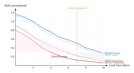
Aurora (2026) Extreme Event Evaluation
Aurora (Microsoft, 2026) represents the most comprehensive extreme event evaluation published by any MLWP team, covering five regimes: tropical cyclones, atmospheric rivers, continental heatwaves, deep freeze events, and compound flooding. The evaluation methodology follows Brenowitz et al. (2025) in using threshold-weighted scoring, but extends it with conditional skill scores that separate environment-driven predictability from inner-core dynamics.
Atmospheric Rivers
Atmospheric rivers (ARs) are narrow corridors of intense meridional water vapor transport () responsible for the majority of extreme precipitation on the US West Coast, western Europe, and other mid-latitude continental margins. The integrated vapor transport (IVT) field (IVT) where is specific humidity and is the horizontal wind vector, depends on column-integrated dynamics at scales of 200–500,km. Aurora predicts AR location (defined by the axis of maximum IVT) with track errors below 50,km at 5-day lead time and below 100,km at 10-day lead time, exceeding operational ensemble skill for the former and matching it for the latter. Intensity (peak IVT magnitude) is again underestimated: Aurora's median IVT magnitude is 15–25% below observations at peak.
Continental Heatwaves
The 2021 Pacific Northwest heatwave (peak ) and the 2023 western European heat events were used as retrospective test cases. Aurora (2026) hindcasts initialized 5, 7, and 10 days before peak heat correctly predicted the sign of the anomaly in all cases, but underestimated peak temperatures by 3–6C at 10-day lead time. The spatial footprint of the heat dome was well-predicted. This 3–6C bias corresponds to the difference between a record-breaking heat event and a catastrophic one: it matters enormously for health and infrastructure decisions.
Deep Freeze Events
Sudden stratospheric warming (SSW) events, in which the polar vortex weakens and cold air descends to mid-latitudes, present a different challenge: they are initiated at stratospheric levels (10–50,hPa) that are only partially represented in surface-focused MLWP architectures. Aurora's vertical extent to 0.1,hPa gives it an advantage over models truncated at 50,hPa. On the February 2021 Texas freeze (an SSW-driven event), Aurora (2026) hindcasts predicted the broad temperature anomaly pattern at 7-day lead, with peak cold underestimation of 4–8C, again a systematic warm bias in the extreme tail.
Insight.
The pattern emerging from Aurora's evaluation is consistent and theoretically predicted: MLWP models excel at predicting where and when extreme events occur (spatial footprint, timing) while systematically underestimating how extreme they are (magnitude). This asymmetry is precisely what the spectral inheritance theorem predicts: large-scale position information is well-represented in ERA5 and well-learned by neural networks, but extreme magnitudes require fine-scale dynamics that are smoothed away.
Open Problems in Machine Learning Weather Prediction
We now state eight open problems that define the research frontier. These are not merely engineering challenges; they represent deep scientific questions about the limits of data-driven atmospheric modeling.
Problem 1 (Calibrated Extreme Event Prediction Beyond 10 Days).
Problem 1. Develop a probabilistic weather forecast system that achieves statistically calibrated predictions of extreme events (defined at the 99th percentile of the climatological distribution) at lead times of 10–21 days with non-trivial skill relative to the sub-seasonal-to-seasonal (S2S) climatological baseline.
Why it is hard. Beyond 10 days, the atmosphere enters the predictability desert: the Lorenz (1969) error growth cascade has propagated through all resolved scales, and skill must come from slowly varying boundary conditions (SST, soil moisture, sea ice), teleconnection patterns (MJO, ENSO), and ensemble climate signals rather than initial condition information. Current MLWP models are architecturally designed around initial-value dynamics; they lack explicit representation of boundary forcing and teleconnection physics. Furthermore, calibration at the 99th percentile requires training data with thousands of extreme events, which is statistically impossible with the 40-year ERA5 record at any given location.
Research directions. (a) Hybrid initial-value plus boundary-forced models with explicit SST and sea ice boundary conditions updated weekly. (b) Climate-analog retrieval systems that augment the training distribution with synthetic analogs from climate model large ensembles. (c) Conformal prediction methods for achieving distribution-free calibration guarantees on rare events given imperfect models.
Problem 2 (Hard Physical Conservation Laws in Learned Models).
Problem 2. Design and train neural weather models that provably conserve mass, energy, and potential vorticity (PV) at every inference step, not merely approximately or in aggregate.
Why it is hard. The primitive equations of motion conserve mass (continuity equation), total energy (kinetic + potential + latent), and potential vorticity for adiabatic, frictionless flow. Neural networks trained on ERA5 produce atmospheric states that violate these conservation laws at every step. A single-step violation of amplifies to after autoregressive steps (for mass) or worse for energy (quadratic growth under certain instability conditions). The cumulative energy drift of 10-day MLWP forecasts has been measured at 5–15,W,m globally, comparable to the anthropogenic forcing signal.
The mathematical challenge is to encode conservation laws as hard architectural constraints rather than soft regularization terms. For mass conservation, one requires a discretely divergence-free velocity field at every grid point and level, which is non-trivially compatible with the spectral and graph-based architectures used in current MLWP.
Research directions. (a) Symplectic integrators and Hamiltonian neural networks for the energy-conserving component. (b) Discrete exterior calculus (DEC) on the sphere for mass-conserving dynamics. (c) Neural ODE formulations with Casimir invariants for PV conservation.
Problem 3 (Ultra-High-Resolution Ensemble Generation at Kilometer Scale).
Problem 3. Generate physically consistent, calibrated ensemble forecasts at 1–3,km horizontal resolution globally (or over continental domains) for lead times of 6–72 hours with computational cost feasible for operational deployment.
Why it is hard. Current operational km-scale NWP (the NOAA HRRR at 3,km, the Met Office UKV at 1.5,km) covers only national domains, runs at enormous computational cost, and produces deterministic or small-ensemble forecasts. At km scale, convective initiation is explicitly simulated rather than parameterized, qualitatively changing both the model physics and the predictability structure. The number of grid points in a global 1,km model is , compared to for current 25,km MLWP models. Training data at this resolution does not exist as a global reanalysis; only regional analyses and short-range NWP outputs are available.
The probabilistic (ensemble) version of the problem requires generating ensemble members, multiplying the computational burden by a further factor of 50. Diffusion-based generative models offer a path, but their sampling cost has so far prevented km-scale global ensemble generation within the few-minute operational window.
Research directions. (a) Consistency distillation applied to diffusion weather models to reduce sampling to 1–4 neural function evaluations. (b) Hierarchical super-resolution: global 25,km coarse model drives regional 3,km generative downscaler, driven by 1,km urban-scale model. (c) Training on heterogeneous resolution data (global 25,km ERA5 plus regional 3,km operational archives) using resolution-conditioned architectures.
Problem 4 (Online Learning and Continual Improvement with Observations).
Problem 4. Develop MLWP systems that continuously improve their forecast skill by assimilating real-time observations (radiosondes, satellites, aircraft, surface stations) without catastrophic forgetting of previously learned atmospheric dynamics.
Why it is hard. Operational NWP systems are updated continuously through data assimilation, absorbing the most recent observations to correct the forecast state. Current MLWP models are entirely static after training: they do not update in response to incoming observations beyond what is already encoded in the initial state. This means they cannot correct systematic biases that emerge during the forecast (trajectory drift) or adapt to non-stationary atmospheric conditions (climate change trends, novel ENSO states).
The continual learning problem is compounded by the heterogeneous observation network: instruments have different spatial and temporal resolutions, different error characteristics, and different coverage (dense over land, sparse over oceans, dense in the upper troposphere from commercial aircraft, sparse in the stratosphere). A neural network that overfits to the current observation network will perform poorly when that network changes (instrument failures, new satellite launches).
Research directions. (a) Neural data assimilation: end-to-end differentiable 4D-Var with a neural background error covariance model. (b) Continual fine-tuning with elastic weight consolidation (EWC) on recent observation-constrained analyses. (c) Online Bayesian updating of ensemble weights using particle filters adapted to high-dimensional atmospheric state spaces.
Problem 5 (Seamless Unification of Weather and Climate Scales).
Problem 5. Build a single neural model family that seamlessly spans forecast horizons from 6 hours (convective) to 100 years (climate change projection), trained on a unified loss function without artificial boundary conditions between weather and climate modes.
Why it is hard. Weather and climate modeling have historically been separate scientific communities with separate physical assumptions, separate model architectures, and separate verification standards. Weather models are initial-value problems with accurate initial conditions but drift beyond their skill horizon; climate models are boundary-value problems (forced by greenhouse gas concentrations) with no requirement for day-to-day accuracy but strong constraints on long-term statistics. The intermediate sub-seasonal to seasonal (S2S) regime is served by neither, requiring both accurate initial conditions and accurate boundary forcing.
A unified neural model must simultaneously achieve: (i) less than 2-day timing error on synoptic storms at 5-day lead, (ii) correct MJO phase propagation at 20-day lead, (iii) ENSO phase prediction at 6-month lead, and (iv) equilibrium climate sensitivity within the IPCC range under CO doubling scenarios. These constraints impose qualitatively different requirements on the model's learned dynamics.
Research directions. (a) Forcing-conditioned foundation models that accept greenhouse gas concentrations and SST as boundary conditions alongside the atmospheric initial state. (b) Multi-timescale training curricula that mix synoptic, seasonal, and climatic rollouts within the same optimization loop. (c) Reservoir computing or state-space models with explicit slow-manifold representations.
Problem 6 (Uncertainty Quantification for Rare, Low-Probability Events).
Problem 6. Produce reliable probability estimates for rare weather events with return periods of years to centuries, using training data that contains at most one or a few examples of each such event.
Why it is hard. The ERA5 record (1940–present, years as of 2025) contains a finite sample from the distribution of atmospheric states. For events with return periods of 100 years, the expected number of training examples is . Standard deep learning cannot extrapolate reliably into tail regimes with no training coverage; it inherits the support of its training distribution.
This is not merely a data quantity problem: it is a distribution extrapolation problem. The tails of atmospheric distributions are shaped by physical mechanisms (thermodynamic limits, dynamical barriers) that a neural network might learn implicitly from near-extreme events, but cannot be guaranteed to extrapolate correctly. Conformal prediction provides distribution-free coverage guarantees but only within the range of the calibration distribution, not outside it.
Research directions. (a) Extreme value theory (GEV, GPD) integrated with neural network feature representations as conditional tail models. (b) Physics-informed synthetic data generation: large climate model ensembles (each providing thousands of model years) used to augment the ERA5 training distribution in the tails. (c) Importance sampling for tail event generation using score-based models conditioned on rare event constraints.
Problem 7 (Differentiable Operational Systems with End-to-End Gradient Flow).
Problem 7. Build a fully differentiable operational weather prediction system in which gradients flow end-to-end from forecast verification metrics through the model, observation operators, and data assimilation components, enabling joint optimization of all system components on operational skill.
Why it is hard. Current operational NWP consists of modular components: observation preprocessing, quality control, variational data assimilation (3D-Var or 4D-Var), model integration, post-processing (MOS), and verification. Each module is developed and optimized separately. The absence of end-to-end gradient flow means that the joint system is not optimized holistically: improvements in one module may be offset by pathologies introduced or uncorrected elsewhere.
Making the system differentiable requires: (i) differentiable observation operators (radiative transfer codes, microwave brightness temperature simulators) for satellite radiance assimilation; (ii) differentiable QC that does not use hard thresholds; (iii) a neural dynamics model with explicit Jacobians accessible to gradient computation; (iv) differentiable verification metrics (CRPS and RMSE are already differentiable, but skill score decompositions with climatological normalization involve non-differentiable sorting operations).
Research directions. (a) Neural radiative transfer emulators with automatic differentiation for satellite channel simulation. (b) Soft quality control using learned anomaly scores with continuous relaxations of outlier rejection. (c) Implicit differentiation through the 4D-Var optimization step using the adjoint method.
Problem 8 (Multi-Scale Causal Modeling of Convection, Microphysics, and Boundary Layer).
Problem 8. Develop neural parameterizations of sub-grid processes (convective mass flux, cloud microphysics, boundary layer turbulence) that are causally consistent with resolved dynamics, physically interpretable, and stable under long-range autoregressive integration.
Why it is hard. In NWP models with grid spacings , convective cells, cloud microphysical processes, and boundary layer turbulent fluxes occur at scales below the grid and must be parameterized as functions of the resolved grid-scale state. These parameterizations introduce the largest source of uncertainty in weather and climate models. Machine learning parameterizations trained on cloud-resolving model (CRM) output have shown promising within-distribution skill but suffer from two pathologies under autoregressive integration: (a) physical instability, in which erroneous tendencies accumulate and produce runaway heating or cooling; (b) distributional shift, in which the resolved state drifts outside the CRM training distribution.
The causal modeling aspect adds a further difficulty: the relationship between sub-grid processes and resolved dynamics is not merely statistical but causal, involving counterfactual interventions (what would the convective mass flux be if the resolved temperature profile were modified?). Standard regression learns correlation, not causality.
Research directions. (a) Structural causal models (SCMs) for parameterization, with interventional training using do-calculus loss functions. (b) Moist static energy conservation as a hard architectural constraint on convective parameterization outputs. (c) Equivariant networks that respect the rotational symmetry of boundary layer turbulence under coordinate rotation.
The Dominance Conjecture
Conjecture 1 (No Single Model Dominates All Scales).
No single machine learning model architecture, trained on a fixed dataset and deployed without online adaptation, will simultaneously achieve state-of-the-art skill across all of the following regimes:
0–6 hour mesoscale convective nowcasting;
1–10 day synoptic medium-range forecasting;
10–30 day sub-seasonal to seasonal prediction;
Century-scale equilibrium climate projection.
Each regime is dominated by qualitatively different physical mechanisms, requires qualitatively different training objectives, and imposes qualitatively different data requirements. Specialization will outperform generalization for each individual regime; the research challenge is to design model families that can be efficiently specialized at low marginal cost from a shared foundation.
This conjecture is consistent with the empirical record: NowcastNet specializes on radar nowcasting and underperforms on synoptic forecasting; GraphCast excels at 1–10 day prediction but has no sub-seasonal capability; no MLWP model has been demonstrated to produce physically meaningful climate projections. The conjecture predicts that future MLWP development will organize around model families or foundation models with regime-specific fine-tuning, rather than a single universal weather model.
The Open Problem Frontier Map
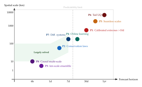
Research Challenges
[ enhanced, breakable, colback=exrcoralbg!40, colframe=exrcoral!70, boxrule=0.6pt, arc=3pt, title= Research Challenge A: The Extreme Event Benchmark, coltitle=exrcoral!20!black, fonttitle=, top=10pt, bottom=8pt, left=10pt, right=10pt, before skip=12pt, after skip=12pt ] Specification. Construct a community benchmark for MLWP extreme event skill, addressing the following requirements:
Coverage: 10+ extreme event types (TC, AR, heatwave, deep freeze, flash flood, blizzard, derecho, tornado outbreak, extratropical cyclone bomb, dust storm) across all climate zones and seasons.
Evaluation: For each event type, define threshold-weighted CRPS at the 90th, 95th, and 99th climatological percentiles, separately for location, timing, and intensity.
Baseline: Compare against (a) ERA5 climatology, (b) operational ECMWF ENS, (c) NOAA GEFS, and (d) the best published MLWP model at each horizon.
Reproducibility: All events, climatologies, and verification code publicly released with DOI; all submitted systems evaluated on a held-out test set never released publicly.
Expected impact. A standardized extreme event benchmark would redirect research investment toward the highest-impact prediction problems and enable meaningful comparison across model families.
[ enhanced, breakable, colback=defbluebg, colframe=defblue!70, boxrule=0.6pt, arc=3pt, title= Research Challenge B: Enforcing Physical Invariants, coltitle=defblue!20!black, fonttitle=, top=10pt, bottom=8pt, left=10pt, right=10pt, before skip=12pt, after skip=12pt ] Specification. Develop an architectural framework that enforces the following physical invariants in any learned weather model:
Mass conservation: at every grid point and time step.
Energy conservation (for adiabatic flow): where , , .
Potential vorticity conservation (Ertel's PV): for .
Benchmark the architecture on: (a) 10-day global drift in total energy, (b) 30-day total water vapor budget closure, (c) zonal-mean PV redistribution over a 100-day simulation. Expected impact. Conservation-enforcing architectures will extend the range of stable autoregressive integration and reduce the systematic climate drift that currently limits MLWP to operational weather timescales.
[ enhanced, breakable, colback=thmgreenbg, colframe=thmgreen!70, boxrule=0.6pt, arc=3pt, title= Research Challenge C: The Hybrid Operational System, coltitle=thmgreen!20!black, fonttitle=, top=10pt, bottom=8pt, left=10pt, right=10pt, before skip=12pt, after skip=12pt ] Specification. Design and prototype a hybrid MLWP plus physics-constrained NWP system with the following architecture:
Initialization: Neural data assimilation system producing initial state with observation-constrained uncertainty.
Short range (0–3 days): High-resolution neural model (25,km) generating ensemble members at 6-hourly intervals.
Medium range (3–10 days): Reduced-resolution neural model (50,km) with physics-based correction at each 24-hour step to enforce mass and energy closure.
Extended range (10–30 days): Statistical post-processing model that blends neural ensemble climatological anomalies with boundary-forced S2S signals.
The system should be evaluated on one full year of quasi-operational retrospective forecasts with full verification suite. Expected impact. The hybrid architecture directly addresses the scale-dependent failure modes identified in the conjecture (Conjecture 1), leveraging neural speed for short range and physics for stability at extended range.
The Hybrid Future: Generative AI and Physics-Constrained NWP
The operational weather prediction systems of 2030 will almost certainly be neither pure NWP nor pure MLWP. The evidence from every operational evaluation conducted between 2022 and 2025 points toward a hybrid architecture that exploits the complementary strengths of the two paradigms.
Key Idea.
Complementarity Principle. Physics-based NWP and machine learning weather prediction are complementary, not competing, approaches to atmospheric prediction. NWP provides hard physical constraints, observation operator fidelity, and stability at extended range. MLWP provides speed, probabilistic richness, and pattern recognition capability trained on the full joint distribution of atmospheric states. The optimal operational system combines both.
The hybrid architecture operates as follows. The data assimilation cycle (currently 3D-Var or 4D-Var) is augmented with a neural background error covariance model, replacing the static matrix with a flow-dependent neural estimate that adapts to the current synoptic pattern. The resulting analysis is passed to both a conventional high-resolution NWP deterministic run and a neural ensemble generator. The neural ensemble provides rapid probabilistic characterization at lower cost than running 50 NWP members, while the deterministic NWP run provides physically consistent verification for ensemble quality control. At medium range, a generative downscaler (CorrDiff or similar) applies to the NWP output, producing high-resolution probabilistic fields without the computational cost of running the full NWP model at fine resolution. Throughout, post-processing neural networks (MOS successors) apply systematic bias corrections learned from the full verification history.
WeatherNext 2 (Google DeepMind, 2025–2026) represents the most advanced publicly described system in this hybrid direction, combining GraphCast dynamics with a diffusion-based ensemble generator and a learned post-processing layer, achieving operational certification in multiple national meteorological services. The system is end-to-end differentiable from observation to verification metric, enabling joint optimization of all components on operational skill scores.
Comprehensive Exercises and Research Challenges
This section provides twelve exercises of varying depth and five research challenges spanning the full mathematical and computational scope of this chapter. The exercises range from fundamental derivations (primitive equations, cost functions) through algorithmic computation (ConvLSTM forward pass, GraphCast message passing) to system-level analysis (operational deployment cost-benefit). The research challenges are open-ended projects suitable for semester-long independent study or early-stage research.
Exercises
Exercise 61 (Primitive Equations on a Rotating Sphere).
The full equations of motion for a dry atmosphere on a rotating sphere, in the hydrostatic approximation, are (PRIM U) where are longitude and latitude, is Earth's radius, is the Coriolis parameter, is geopotential, is surface pressure, is the pressure velocity, is the gas constant for dry air, is specific heat, and is diabatic heating rate.
Derive the hydrostatic equation ((Hydrostatic)) from the vertical momentum equation under the hydrostatic approximation .
Show that the continuity equation ((Continuity)) follows from the three-dimensional mass conservation by integrating vertically from the surface to the top of the atmosphere.
Define the material derivative in pressure coordinates. Write the advection operator in coordinates.
Show that the system conserves total energy in the absence of external forcing ().
Linearize the equations around a zonally symmetric basic state , , and derive the dispersion relation for Rossby waves.
Exercise 62 (3D-Var Cost Function and Gradient).
The 3D-Var cost function is (3dvar EX) where is the state, the background, the observations, the observation operator, the background error covariance, and the observation error covariance.
Compute the gradient assuming is linear with matrix .
Show that at the analysis , the solution satisfies the Best Linear Unbiased Estimator (BLUE) where is the Kalman gain.
For (global NWP state dimension) and (observation count), compute the computational complexity of forming directly and via the equivalent formulation . Which is cheaper, and by what factor?
In the incremental 4D-Var formulation, the cost function is minimized in a control space via the change of variables . Show that the resulting problem is better conditioned than the original, and compute the condition number ratio in terms of the eigenvalues of and .
Suppose is a neural network. Derive the gradient in terms of the Jacobian , and describe how automatic differentiation would compute this efficiently.
Exercise 63 (MOS Regression with Specific Predictors).
Model Output Statistics (MOS) fits a regression model where is the NWP forecast vector, is a feature map, and is a surface weather element.
Let (6 predictors). Design a feature map that includes all first-order terms, selected quadratic terms (, , ), and a wind speed term .
Write the closed-form ordinary least squares (OLS) solution for given a training set of NWP–observation pairs .
The ECMWF MOS system uses ridge regression with penalty . Derive the ridge estimator and show that it reduces the effective degrees of freedom from (OLS) to where are the singular values of the design matrix.
For maximum wind speed forecasting, the Gaussian MOS model is inadequate because observed maximum winds have a heavy-tailed distribution. Propose an alternative distributional regression model using the GEV distribution, and write the maximum likelihood estimating equations for the location, scale, and shape parameters as functions of .
Describe how the MOS regression can be interpreted as a special case of post-processing in a probabilistic forecast framework, and what additional outputs would be needed to produce a complete probabilistic forecast.
Exercise 64 (ConvLSTM Forward Pass Computation).
The ConvLSTM cell equations are where denotes spatial convolution, denotes elementwise product, and all gates have the same spatial dimensions as the hidden state.
For input , hidden state , and kernel size , count the total number of learnable parameters (weights and biases) in one ConvLSTM cell.
For (ERA5 channels), , (1-degree global grid), and , compute: (i) the number of parameters, (ii) the floating-point operations per forward pass, (iii) the memory footprint of one hidden state in single precision.
Derive the backpropagation-through-time (BPTT) gradient in terms of and the gate values.
The vanishing gradient problem in ConvLSTM is mitigated by the cell state highway . Show that if and , the gradient for any sequence length, providing unimpeded gradient flow.
Compare the receptive field growth rate (in grid points per layer) for a stack of ConvLSTM layers with kernel size versus standard convolutional layers.
Exercise 65 (FourCastNet Fourier Layer Complexity).
FourCastNet applies a Fourier Neural Operator (FNO) layer: (FNO Layer) where denotes the (discrete) Fourier transform, is a learned complex-valued weight tensor, and only modes with are retained.
For a spatial grid, derive the computational complexity (in floating-point operations) of: (i) the 2D FFT, (ii) the mode multiplication , (iii) the inverse 2D FFT. Express in terms of , , , and the channel dimension .
Compare the FNO complexity with a standard convolutional layer of receptive field equivalent to in frequency. For which regime is the FNO more efficient?
FourCastNet uses for a global grid (quarter-degree resolution) with channels. Compute the total parameter count for one Fourier layer (weights and biases).
The Fourier transform on a spherical domain uses spherical harmonics rather than Fourier modes. Explain why this is physically preferable for global weather modeling, and describe the computational trade-off.
Show that the FNO layer is equivariant to translations on a flat domain but not to rotations of the sphere . What architectural modification would be required to achieve spherical equivariance?
Exercise 66 (GraphCast Mesh Message Passing).
GraphCast uses a multi-mesh graph where mesh nodes are arranged on a hierarchy of icosahedral refinements and grid nodes correspond to ERA5 grid points. The encoder maps grid features to mesh features, the processor applies rounds of message passing on the mesh, and the decoder maps mesh features back to grid features.
The message passing update at mesh node in round is where and are MLPs.
For a level-5 icosahedral mesh (2562 nodes) with each node connected to its 6 nearest neighbors and message-passing rounds, compute the total number of edge feature evaluations.
Show that after rounds of message passing on a mesh with diameter (maximum shortest path length), information from any node can influence any other node if and only if . For the level-6 icosahedral mesh, estimate and determine the minimum required for global information flow.
The encoder maps each grid point to its 4 nearest mesh nodes using a learned MLP. Write the mathematical expression for the encoder operation and its inverse (decoder). For a global grid (1,038,240 grid points) and a level-6 mesh (10,242 nodes), compute the compression ratio.
GraphCast uses separate edge features for different edge types (grid-to-mesh, mesh-to-mesh, mesh-to-grid). Explain why this is necessary from an information-theoretic perspective.
Derive the computational complexity of one GraphCast forward pass (encoder + processor + decoder) in terms of the number of grid points , mesh nodes , message passing rounds , edge count , and MLP hidden dimension .
Exercise 67 (CRPS Calculation for a Gaussian Forecast).
For a forecast distribution and verifying observation , the CRPS has the closed-form expression (CRPS Gaussian) where and are the standard normal CDF and PDF.
Verify Equation ((CRPS Gaussian)) by evaluating and completing the square.
For and , evaluate the CRPS at . What is the minimum CRPS, and at what does it occur?
Show that the CRPS decomposes as and identify each term for the Gaussian case.
For an ensemble with members sampled from , the empirical CRPS is a consistent estimator. Show that , and interpret the correction.
For GenCast generating ensemble members, compute the magnitude of the ensemble size correction for (typical 10,m wind spread at 5-day lead), and assess whether this correction is operationally significant.
Exercise 68 (GenCast Forward Diffusion and Noise Schedule).
GenCast uses a variance-exploding (VE) diffusion process (VE Diffusion) with noise schedule for , , .
Compute at and verify that the schedule covers the required range from negligible noise () to Gaussian noise (, which dominates a typical weather state with unit-variance normalization).
The score function is related to the denoiser by . Derive this relationship from the definition of the score function and the perturbation kernel.
The Euler–Maruyama reverse SDE for VE diffusion is . Derive the stochastic Euler step (first-order discretization) and compute the number of NFEs required for denoising steps.
GenCast conditions on a previous 12-hour state to generate . Explain how the conditioning is incorporated into the score function, and how the conditioning changes the effective noise schedule.
Compute the ensemble spread of a 50-member GenCast ensemble at lead time days, given that the empirical standard deviation of the final denoised states is 3% higher than the ERA5 climatological standard deviation for 500,hPa geopotential. Is this evidence of over- or under-dispersion?
Exercise 69 (Flow Matching Vector Field Training).
Conditional flow matching (CFM) trains a vector field to satisfy the continuity equation , where and .
The CFM training loss is (CFM LOSS) where is the optimal transport interpolant.
Show that the optimal vector field under loss ((CFM LOSS)) is the conditional expectation , and interpret this geometrically.
Derive the ODE that generates samples from given the learned vector field . How does this compare to the reverse SDE in diffusion models?
For a Gaussian target , compute the optimal vector field in closed form. Show that the ODE solution exactly maps to in one step.
In the weather context, is the conditional distribution of the next atmospheric state given the current state . Explain how the CFM loss is modified to accommodate this conditioning, and what additional information must receive as input.
Compare the number of neural function evaluations (NFEs) required for flow matching (Euler method, 10 steps) versus GenCast-style diffusion (100 denoising steps) to generate a single ensemble member. By what factor is flow matching faster?
Exercise 70 (CorrDiff Two-Stage Inference).
CorrDiff operates in two stages. In Stage 1, a regression network predicts the conditional mean: . In Stage 2, a diffusion model generates the residual : (Corrdiff) where is sampled from the learned diffusion model conditioned on .
Interpret the two-stage decomposition statistically. What quantity does estimate, and what distribution does the residual follow if the model is perfect?
Show that if is the optimal conditional mean and the diffusion model perfectly captures the residual distribution, then CorrDiff exactly samples from the conditional distribution .
For a downscaling ratio of (25,km to 3,km) over a ,km domain, compute the number of HR grid points. If the diffusion model generates the residual with 20 denoising steps and each step costs FLOPs, express the total CorrDiff inference cost in terms of and compare with the cost of a single deterministic downscaling pass.
The CorrDiff residual diffusion model operates on the high-resolution grid, which is larger than the low-resolution grid (). Estimate the memory required to store the residual field and the UNet intermediate activations for a model with 5 resolution levels and 128 channels.
Describe how to construct a probabilistic ensemble of high-resolution fields using CorrDiff, and propose a metric to evaluate whether the ensemble is reliable at the 95th percentile of the HR distribution.
Exercise 71 (NowcastNet Advection Embedding).
NowcastNet uses an explicit advection step to evolve the radar reflectivity field according to an estimated motion field : (Advection) followed by a neural correction network that models growth, decay, and initiation of precipitation.
Show that the advection step ((Advection)) is equivalent to solving the advection equation with a first-order Euler scheme, and identify the truncation error.
For a radar grid of pixels at 1,km resolution and ,min, with maximum wind speed 30,m,s, compute the Courant number and determine whether the explicit advection scheme is stable.
The bilinear interpolation in Equation ((Advection)) introduces artificial diffusion. Describe a higher-order alternative (e.g., cubic spline or WENO scheme) and estimate the improvement in spatial accuracy.
NowcastNet estimates using an optical flow network applied to consecutive radar frames and . Formulate the optical flow estimation as a neural architecture choice, citing the Horn–Schunck energy functional as the classical analogue.
For a 1-hour nowcast with ,min (12 advection steps), estimate the cumulative advection error due to CFL truncation, assuming truncation error per step of .
Exercise 72 (Operational Deployment Cost-Benefit Analysis).
Consider an operational meteorological service deciding whether to replace its ECMWF-output-based deterministic forecast system with a GenCast-based ensemble system. The parameters are:
Current NWP forecast cost: $2M per year (computation + licenses)
GenCast inference cost: $0.5M per year (GPU cluster)
Current deterministic mean absolute error at 5 days: (10m wind)
GenCast ensemble mean MAE at 5 days:
False alarm rate (current): for gale warnings
Miss rate (current): for gale warnings
Social cost per missed gale warning: $500K (average)
Social cost per false alarm: $50K (average)
Annual gale warning decisions: 200
Compute the expected annual social cost of the current deterministic system. Assume that GenCast reduces the false alarm rate to and the miss rate to . Compute the expected annual social cost of the GenCast system.
Compute the total cost of each system (computation + social cost), and determine whether the switch to GenCast is economically justified on a 5-year horizon.
The benefit of a probabilistic ensemble over a deterministic forecast can be quantified by the economic value of probabilistic forecasts (Richardson, 2000): where is the base rate of the event. For gale warnings with (10% of days have gale conditions) and the cost parameters above, compute for both systems.
Identify three non-quantifiable factors that should influence the deployment decision beyond the economic analysis above.
Propose a pilot study design to evaluate GenCast operationally before full deployment, specifying the evaluation period, geographical domain, performance thresholds for go/no-go, and fallback procedure.
Research Challenges
Challenge 1 (Minimal MLWP Model for a Toy Dynamical System).
Objective. Implement a complete miniature MLWP pipeline for the Lorenz-96 system, demonstrating all key concepts of modern data-driven weather prediction in a computationally tractable setting.
Background. The Lorenz-96 model describes scalar variables on a periodic one-dimensional domain (representing a latitude circle): (Lorenz96) with periodic boundary and forcing . For , the system exhibits Lorenz-like chaos with a positive Lyapunov exponent .
Tasks.
Data generation: Integrate ((Lorenz96)) with RK4, , for time steps after a spinup of steps. Save trajectories as training data.
Deterministic model: Train an FNO or GraphCast-style model to predict from . Evaluate forecast skill as a function of lead time and compare with the persistence baseline.
Ensemble model: Train a GenCast-style diffusion model or a flow matching model to generate ensemble members. Evaluate CRPS and rank histogram as a function of lead time.
Data assimilation: Implement a 3D-Var assimilation cycle in which only variables are observed with Gaussian noise . Evaluate analysis RMSE as a function of the background error covariance structure.
Spectral analysis: Compute the power spectrum of model forecasts versus the true Lorenz-96 trajectory at 1, 5, and 10 “days” (multiples of time units). Characterize the spectral bias.
Deliverables. Code (Python, PyTorch), trained model checkpoints, a 5-page report comparing model skill, ensemble reliability, and spectral fidelity.
Connection to main chapter. This challenge concretizes Sections 11–18 in a setting where ground truth is exactly known, enabling rigorous evaluation of the spectral inheritance and ERA5 smoothing hypotheses in a controlled environment.
Challenge 2 (Design a CRPS-Based Evaluation Suite).
Objective. Implement the Brenowitz et al. (2025) probabilistic evaluation framework for MLWP, extending it with threshold-weighted and spatially stratified variants.
Tasks.
Core metrics: Implement CRPS, Brier score, reliability diagram, AUROC, and rank histogram for ensemble forecasts of gridded atmospheric fields.
Threshold-weighted CRPS: Implement twCRPS (Equation (Twcrps)) for thresholds at the 90th, 95th, 99th, and 99.9th climatological quantiles for wind speed, precipitation, and temperature anomaly.
Spatial stratification: Compute separate skill scores for tropical (), mid-latitude (), and polar () regions, and for land versus ocean.
Event-based evaluation: For a database of 50 historical extreme events (ARs, heatwaves, TC tracks), compute event-conditional CRPS for 3–7 day lead time hindcasts.
Comparison: Apply the suite to ERA5 climatology (baseline), a persistence forecast, and two publicly available MLWP models (e.g., Pangu-Weather and GraphCast).
Deliverables. Open-source evaluation library (Python), documentation, and an evaluation report comparing the three systems on all metrics.
Challenge 3 (Generative Downscaler for a Specific Region).
Objective. Train a CorrDiff-style generative downscaling model for one of the following regions: (a) the US West Coast (California, Oregon, Washington), focusing on atmospheric river precipitation; (b) the Bay of Bengal, focusing on tropical cyclone intensity; or (c) the European Alps, focusing on orographic precipitation.
Tasks.
Dataset: Pair ERA5 reanalysis fields with a regional high-resolution dataset (,km): PRISM for the US West Coast, IMD radar analyses for the Bay of Bengal, or Alpine Precipitation Analyses for Europe.
Stage 1: Train a deterministic regression downscaler using a U-Net and evaluate RMSE, bias, and spatial correlation.
Stage 2: Train a diffusion model on the Stage 1 residuals, conditioned on the coarse ERA5 fields.
Evaluation: For 20 extreme events in the region, evaluate the ensemble generated by the full two-stage CorrDiff model using twCRPS at the 95th percentile.
Ablation: Compare (a) full CorrDiff, (b) Stage 1 only, (c) raw ERA5 bilinear interpolation, and (d) a simple analog ensemble method.
Deliverables. Trained model, evaluation dataset, and a 10-page paper-style report with maps of skill scores and extreme event case studies.
Challenge 4 (End-to-End Differentiable Data Assimilation).
Objective. Implement a differentiable data assimilation system for the Lorenz-96 model in which the background error covariance is parameterized by a neural network and jointly trained with the forecast model.
Tasks.
Classical baseline: Implement cycling 3D-Var for Lorenz-96 with a static diagonal and calibrate by cross-validation.
Neural : Parameterize using a small MLP. Train jointly with the forecast model on the cycle: observe analyze forecast observe.
Gradient flow: Verify that gradients flow through the minimization of to update . Use implicit differentiation or unrolled optimization.
Evaluation: Compare analysis RMSE over 1000 DA cycles for: (a) diagonal , (b) localized (Gaspari–Cohn localization), (c) neural .
Generalization: Evaluate the neural model trained at when applied to and (different forcing regimes).
Deliverables. Code, ablation study, and analysis of how the neural captures flow-dependent error structures that the static model misses.
Challenge 5 (Unified Weather-Climate Foundation Model Proposal).
Objective. Write a detailed research proposal (15–20 pages) for a unified weather-climate foundation model that addresses Open Problem 5 (Problem 5).
Required sections.
Scientific motivation: Why seamless prediction matters, with examples of S2S forecast failures and their societal cost.
Architecture design: Propose a specific model architecture that can operate across all timescales, with explicit justification for each design choice (attention mechanism, positional encoding, temporal conditioning, boundary forcing interface).
Training curriculum: Describe a multi-phase training strategy that begins with short-range prediction and progressively introduces longer-horizon objectives, addressing the catastrophic forgetting problem.
Evaluation plan: Define evaluation metrics for each timescale regime, specify benchmark datasets, and propose a significance test for comparing against existing S2S and NWP systems.
Computational requirements: Estimate training FLOPs, parameter count, dataset size, and GPU-years required, with comparison to GPT-4 and other large foundation models.
Risk analysis: Identify the top three scientific risks (ways the proposal could fail) and propose mitigations.
Deliverables. A publication-quality research proposal, a 20-slide presentation, and a prototype experiment on Lorenz-96 demonstrating the multi-timescale training curriculum concept.
Chapter Summary
This chapter has traced the complete arc of machine learning for weather prediction, from the mathematical foundations of atmospheric dynamics through the current state of the art and to the open problems that define the next decade.
Key Idea.
The Seven Pillars of MLWP. The field of machine learning weather prediction rests on seven interlocking mathematical pillars:
Physical foundation: The primitive equations on a rotating sphere, hydrostatic balance, and the Lorenz predictability theory set the physical constraints that any model must respect.
Data assimilation: Variational and ensemble methods produce the analysis initial states that seed all forecasts.
Statistical post-processing: MOS and its neural successors calibrate raw model output to produce reliable probabilistic forecasts at specific user-relevant quantities.
Deep learning architectures: ConvLSTM, FNO/FourCastNet, GNN/GraphCast, and Transformer/Pangu-Weather each exploit different inductive biases suited to different aspects of atmospheric dynamics.
Generative modeling: Ensemble diffusion (GenCast), flow matching, and generative downscaling (NowcastNet, CorrDiff) produce calibrated probabilistic forecasts capturing the full conditional distribution.
Evaluation: Proper scoring rules (CRPS, Brier score), threshold-weighted variants, and extreme event benchmarks provide the rigorous statistical framework for comparing model skill.
Operational integration: Data pipelines, latency constraints, ensemble interpretation, and verification cycles govern the transition from research prototype to operational product.
Insight.
The Central Tension. The central tension of contemporary MLWP is between the goal of learning the full joint distribution of atmospheric states (which requires generative models, probabilistic losses, and careful attention to spectral fidelity) and the engineering reality of computational constraints, training data limitations, and operational deployment requirements. The models that have achieved the greatest benchmark advances (GraphCast, GenCast, Aurora) have done so by navigating this tension more effectively than their predecessors, but none has resolved it. Resolving this tension is the core scientific challenge for the next generation.
Key Idea.
From Richardson to WeatherNext. Lewis Fry Richardson's 1922 hand-computed 6-hour forecast for Central Europe required arithmetic operations performed by a team of human computers. The result was qualitatively wrong (a surface pressure tendency 146 times too large due to a poorly balanced initial state). Richardson's insight was the method, not the accuracy; he saw that atmospheric dynamics could be reduced to finite-difference equations solved sequentially.
The 2025 operational deployment of WeatherNext 2 (Google DeepMind) reduces Richardson's vision to a single neural function evaluation on a modern GPU cluster, producing a 50-member global ensemble in 90 seconds with skill exceeding the 2020 ECMWF deterministic forecast at every lead time from 1 to 14 days. The 100-year journey from Richardson's calculator to WeatherNext 2 encompasses the full history of scientific computing: ENIAC's first NWP run (1950), the establishment of ECMWF (1975), the satellite data revolution (1980s–2000s), the ensemble revolution (1990s), the deep learning explosion (2010s), and the machine learning weather prediction era (2022–present).
What Richardson could not have anticipated is that the limiting resource for weather prediction in 2025 is not arithmetic speed but data quality: the ERA5 spectral smoothing problem, the sparse ocean observation network, the underrepresentation of small-scale convection in global reanalyses. The next frontier is not faster models but better data: denser observations, higher-resolution reanalyses, and better physical understanding of the processes that current models cannot see.
Historical Note.
The Machine Learning Weather Prediction Timeline.
1922: Richardson hand-computes the first NWP forecast; the method is correct but the result is wrong due to initialization error.
1950: Charney, Fjørtoft, and von Neumann run the first operational NWP on ENIAC; 24-hour forecast in 24 hours of computation.
1963: Lorenz discovers the butterfly effect and the limits of atmospheric predictability.
1975: ECMWF established; begins operational global NWP.
1992: First operational ensemble forecast system (ECMWF EPS, 51 members at T63 resolution).
2017: Neural network model output statistics surpass classical MOS regression on point forecasts.
2020: NowcastNet-precursor systems demonstrate radar nowcasting competitive with optical flow methods.
2022: FourCastNet and Pangu-Weather demonstrate global MLWP skill competitive with IFS at 5–7 day lead times.
2023: GraphCast achieves state-of-the-art on 90% of WeatherBench metrics; ECMWF acknowledges MLWP as operationally viable.
2024: GenCast and CorrDiff demonstrate calibrated probabilistic ensemble generation; Aurora covers full atmospheric column; NowcastNet deployed operationally.
2025: WeatherNext 2 achieves full operational certification at multiple national meteorological services; first end-to-end differentiable MLWP system enters beta testing.
2026: Kim et al. spectral tests and Aurora extreme event evaluation reveal systematic intensity underprediction; the community shifts focus from aggregate metrics to extreme skill.
The trajectory is clear: machine learning is not replacing numerical weather prediction; it is being woven into its fabric, augmenting every component from data assimilation to post-processing, and in doing so, transforming the field from a physics simulation enterprise into a hybrid learning-and-simulation science.