40 Federated Learning for Generative Models
Imagine training a diffusion model on everyone's medical records. Now imagine doing it without seeing a single one. This is not a thought experiment-it is the central promise of federated learning for generative models, a discipline born from the collision of two irresistible forces: the insatiable appetite of generative AI for ever-larger training corpora, and the equally inexorable tightening of data privacy law, clinical ethics, and corporate sovereignty across the globe.
In the decade between 2014 and 2024, the default assumption of machine learning shifted from “collect all the data, ship it to a data centre, and train” to something more fraught and more interesting. The Generative Adversarial Network (Goodfellow et al., 2014) required an ImageNet-scale dataset assembled in one place. The original DALL-E (Ramesh et al., 2021) was trained on 250 million image-text pairs scraped from the web. GPT-4 (OpenAI, 2023) consumed, by various estimates, between one and ten trillion tokens, drawn from essentially every freely accessible text document on the internet. The trajectory is unmistakable: generative models grow more capable by consuming more data, and the next frontier of improvement lies in data that cannot be freely assembled-medical records, financial documents, personal communications, industrial sensor streams.
The very moment this data becomes scientifically indispensable, it becomes legally inaccessible. The European Union's General Data Protection Regulation (GDPR, 2018) established the right to erasure, the right to data portability, and strict requirements for lawful processing. The California Consumer Privacy Act (CCPA, 2020) extended analogous protections to the world's fifth-largest economy. The Health Insurance Portability and Accountability Act (HIPAA) in the United States has governed medical data since 1996, and its de-identification requirements make centralised clinical AI training a legal minefield. The EU AI Act (2024), the first comprehensive regulatory framework specifically targeting artificial intelligence, imposes risk-based obligations that make data governance a first-class engineering concern.
The result is a profound paradox: generative models need more data than discriminative models, but data is becoming more restricted. A discriminative model learns a boundary ; it needs enough examples to trace that boundary. A generative model must learn the full joint distribution -or even alone-and must therefore capture the entire support of the data manifold, including rare modes, tail events, and distributional subgroups that a classifier can safely ignore. This requirement for comprehensive coverage scales badly with the fragmentation of data across organisational, geographic, and jurisdictional boundaries.
Federated learning, proposed in its modern form by McMahan et al. (2017) under the name “communication-efficient learning of deep networks from decentralised data,” offers a principled resolution. The insight is architectural: instead of moving data to the model, move the model to the data. Clients train locally on private data; a central server aggregates their updates; no raw data ever leaves its origin. This chapter develops the theory and practice of applying this paradigm to generative models-a much harder problem than the discriminative setting that motivated the original proposal.
The Privacy Paradox of Generative AI
The Data Hunger of Generative Models
The difference in data requirements between discriminative and generative models is not a matter of degree-it is a matter of kind. To understand why, consider a simple binary image classification problem: given an image , predict whether it contains a cat. A classifier needs only to learn a decision boundary that separates cat images from non-cat images. It can, in principle, succeed by memorising a few hundred representative examples from each class. Indeed, transfer learning has made it routine to train effective classifiers on datasets of a few thousand labelled images.
A generative model has no such luxury. It must learn , the full distribution over images. In a -dimensional space with , the support of natural images is a highly curved, low-dimensional manifold embedded in this ambient space. Capturing this manifold faithfully requires training examples that densely sample every region of it-every pose, every lighting condition, every age demographic, every rare anatomical variant in a medical setting.
Quantitatively, the gap is stark. State-of-the-art image classifiers on ImageNet achieve near-human performance trained on 1.2 million examples. The best image generation models require datasets that are two to three orders of magnitude larger: LAION-5B (5 billion image-text pairs), JFT-3B (3 billion images), and CommonCrawl-derived corpora of comparable scale for language models. Every mode of the training distribution that is underrepresented becomes a mode that the model either drops (mode collapse) or distorts.
Key Idea.
A discriminative model learns a boundary ; it needs data dense near that boundary. A generative model must learn the full density ; it needs data dense everywhere in the support. This fundamental difference means generative models are quantitatively and qualitatively more sensitive to dataset size, coverage, and distributional balance than any discriminative counterpart trained on the same task.
This distinction becomes critical when we consider specialised domains. In medical imaging, the “rare disease” problem is endemic: some pathologies appear in fewer than one in ten thousand scans. A classifier trained to detect the most common conditions can afford to be weak on rare ones; a generative model that cannot synthesise rare pathologies authentically is useless for data augmentation precisely where augmentation is most needed.
Similarly, in natural language processing, dialect diversity, domain specificity, and linguistic minority languages are precisely the conditions most undersupplied in any centralised web crawl. A generative model trained on majority-dialect text will systematically fail to model minority variants-not because the architecture is flawed, but because the data was never collected in the first place.
The Regulatory Landscape
The same years that witnessed the explosion of data-hungry generative models also saw the construction of a global regulatory apparatus designed to limit their data supply. We survey the major frameworks here not as lawyers but as engineers who must understand the constraints they impose.
General Data Protection Regulation (GDPR, 2018).
The GDPR, effective May 25, 2018, applies to any processing of personal data of EU residents, regardless of where the processing organisation is located. Its key provisions for machine learning practitioners are:
Lawful basis for processing (Article 6): data may only be processed with explicit consent, for contractual necessity, legal obligation, vital interests, public task, or legitimate interests. Training a generative model on scraped web data satisfies none of these for identifiable individuals.
Right to erasure (Article 17): individuals may request that their data be deleted. For a trained model, this raises the question of “machine unlearning”-can a specific data point's influence be removed from a trained generative model? (Explored in Chapter 29.)
Data minimisation (Article 5): only the minimum necessary data should be collected. This principle directly conflicts with the generative model paradigm of “more data is always better.”
Purpose limitation (Article 5): data collected for one purpose cannot be reused for another. Electronic health records collected for clinical care cannot be freely repurposed for AI training.
Violations carry fines up to 4% of global annual turnover or EUR,20 million, whichever is higher. The GDPR has been enforced: Meta was fined EUR,1.2 billion in 2023 for transferring EU user data to the United States; Amazon was fined EUR,746 million in 2021.
Health Insurance Portability and Accountability Act (HIPAA, 1996/2013).
HIPAA governs Protected Health Information (PHI) in the United States. The HIPAA Privacy Rule (2003) and Security Rule (2005) impose strict access controls on 18 categories of individually identifying health information, including names, geographic identifiers, dates, phone numbers, medical record numbers, and account numbers. The HIPAA de-identification standard (45 CFR 164.514) requires either expert determination (statistical demonstration that re-identification risk is “very small”) or the Safe Harbor method (removal of all 18 identifiers). These requirements make centralised training on electronic health records legally and operationally hazardous.
California Consumer Privacy Act (CCPA, 2020) and CPRA (2023).
The CCPA, enacted in 2020 and strengthened by the California Privacy Rights Act (CPRA) in 2023, grants California residents the right to know what personal information is collected, the right to delete it, and the right to opt out of its sale. California is the world's fifth-largest economy, and compliance with CCPA is effectively mandatory for any technology company with a significant US presence. The CPRA additionally created the California Privacy Protection Agency, the first US data privacy enforcement agency.
EU Artificial Intelligence Act (2024).
The EU AI Act, adopted in March 2024, is the world's first comprehensive regulatory framework specifically targeting AI systems. It establishes a risk-based classification:
Unacceptable risk (prohibited): AI systems for social scoring by governments, real-time remote biometric identification in public spaces, and AI that subliminally manipulates behaviour.
High risk: AI systems in critical infrastructure, education, employment, essential services, law enforcement, migration, and administration of justice. These require conformity assessments, data governance measures, and transparency obligations.
Limited risk: AI systems interacting with humans (chatbots) and those generating synthetic content (deepfakes) must disclose their AI nature.
Minimal risk: all other AI systems, subject only to voluntary codes of conduct.
Generative models used for medical diagnosis, credit scoring, or facial recognition fall squarely in the high-risk category. Foundation models (GPAI, general-purpose AI) with over FLOPs of training compute face additional requirements for transparency, adversarial testing, and incident reporting.
Remark 1.
The regulatory trend is unmistakable and global: Brazil's LGPD (2020), India's DPDP Act (2023), China's PIPL (2021), South Korea's PIPA (amended 2020), and analogous frameworks across the Gulf Cooperation Council are all converging on the same core principles-consent, purpose limitation, data minimisation, and accountability. The question is not whether data privacy regulation will constrain generative AI training; it already does. The question is whether the ML community will adapt by building privacy into the architecture rather than treating it as a compliance checkbox. Federated learning is the most principled answer to that question currently available.
Data at the Edge: The IoT Reality
While regulation restricts the centralisation of existing data, a parallel technological trend is ensuring that an enormous fraction of future data will be generated in locations where centralisation was never viable in the first place.
By 2030, estimates suggest there will be 40 billion Internet of Things (IoT) devices in operation worldwide-smartphones, wearables, industrial sensors, connected vehicles, home appliances, and environmental monitors. These devices collectively generate data at rates that defy centralisation on purely physical grounds. The International Data Corporation projects that the global datasphere-the total amount of data created, captured, copied, and consumed-will reach 200 zettabytes by 2030, with over half of it generated at the edge.
Consider the arithmetic. One zettabyte is bytes. The total capacity of all the world's data centres as of 2023 is approximately 10 zettabytes. Shipping 100 zettabytes of edge-generated data per year to centralised servers would require global network infrastructure two orders of magnitude larger than what exists. It is not merely inadvisable; it is physically impossible.
Definition 1 (Data Silo).
A data silo is a collection of data held by a single entity (a hospital, a device, an organisation, or a jurisdiction) that cannot be directly shared with other entities due to privacy, legal, bandwidth, or sovereignty constraints. Formally, given entities each holding a local dataset , the data is siloed if there is no mechanism by which any entity can observe the raw samples . The aggregate dataset is notionally available but physically inaccessible as a whole.
Data silos exist on multiple scales:
Device-level silos: each smartphone or wearable holds its owner's personal data. A keyboard app generates personalised language data; a health monitor generates biometric time series; a camera generates face images.
Institutional silos: hospitals hold patient records; banks hold financial transaction histories; law firms hold privileged communications.
National silos: data localisation laws in Russia (FZ-242), China (MLPS 2.0), and increasingly other jurisdictions require that personal data on citizens be stored and processed within the country's borders.
Competitive silos: companies with valuable proprietary datasets refuse to share them with competitors even when collaboration would be mutually beneficial scientifically.
The IoT context introduces a further dimension: the data is not merely siloed-it is non-iid (not independently and identically distributed). Each device generates data from a distribution that reflects its owner's personal behaviour, demographics, location, and device characteristics. User 's smartphone keyboard captures their personal vocabulary, writing style, and the topics they discuss; user 's keyboard captures something qualitatively different. When a generative model trained on such heterogeneous data must capture the full joint distribution, this non-iid structure creates profound challenges that we address throughout this chapter.
Why Centralisation Fails
The naive approach to training generative models on siloed data is to centralise it first and worry about the consequences later. This approach fails on four independent grounds, each sufficient on its own.
Privacy failure.
Once data leaves its origin, the centralising entity becomes liable for its protection. Data breaches are not theoretical: the Anthem breach (2015) exposed 78.8 million health records; the Equifax breach (2017) exposed 147 million financial records; the Yahoo breach (2013–2016) exposed 3 billion user accounts. Even in the absence of external attacks, centralised training creates insider threat vectors: researchers, engineers, and infrastructure providers with access to training data have historically exploited it. Moreover, as demonstrated in Chapter 29, even a model trained on centralised data and then published-without releasing the training data-leaks information about individual training examples through membership inference attacks.
Bandwidth failure.
The raw data volume at the edge simply cannot traverse available network infrastructure. A single hospital's PACS (Picture Archiving and Communication System) generates terabytes of imaging data per month. A manufacturing plant with continuous sensor monitoring generates gigabytes per hour. A fleet of autonomous vehicles captures terabytes per vehicle per day. Aggregating these at a central server is not economically or technically feasible at the required scale.
Legal failure.
Moving data across national borders, across institutional boundaries, or between corporate entities creates legal exposure under data protection law, sector-specific regulation, contractual non-disclosure agreements, and national security rules. The Schrems II ruling (2020) invalidated the EU-US Privacy Shield, making routine transatlantic data flows for AI training legally uncertain until the EU-US Data Privacy Framework (2023) was established-and that framework remains contested. Clinical data sharing between hospitals requires data use agreements, IRB approval, and institutional review processes that can take months to years to complete.
Sovereignty failure.
National AI strategies explicitly frame domestic data as a strategic asset. China's Cybersecurity Law (2017) and Data Security Law (2021) prohibit the cross-border transfer of data deemed important to national security or the public interest without government approval. Russia's Federal Law No. 242-FZ requires personal data of Russian citizens to be processed on servers located in Russia. India's Digital Personal Data Protection Act (2023) includes provisions for cross-border data transfer restrictions. In this environment, building generative AI on centralised, globally assembled datasets is not just technically difficult-it is politically untenable for an increasing fraction of the world's data.
The Federated Learning Solution
Federated learning resolves the centralisation dilemma by inverting the direction of movement: instead of moving data to the model, move the model to the data.
The canonical federated learning algorithm, FedAvg (McMahan et al., 2017), operates as follows:
A server initialises a global model with parameters .
In each communication round : enumerate
The server selects a subset of clients, where .
Each selected client receives the current global parameters , runs epochs of local stochastic gradient descent on , and sends back updated parameters .
The server aggregates: (Fedavg) enumerate
The process repeats until convergence.
At no point does any client's raw data leave its local storage. The server and other clients observe only parameter vectors -high-dimensional tensors of floating-point numbers that do not directly encode individual training examples.
Key Idea.
Train the model where the data lives, not the data where the model lives. This inversion of the centralisation paradigm is the foundational principle of federated learning. It trades communication of gradients and parameters for non-communication of raw data, achieving privacy through architecture rather than through post-hoc anonymisation, which as Chapter 29 demonstrates, is rarely sufficient.
A Brief History of Federated Learning
Historical Note.
From FedAvg to Federated Foundation Models. The term “federated learning” was coined by McMahan, Moore, Ramage, Hampson, and Aguera y Arcas in a 2017 paper, “Communication-Efficient Learning of Deep Networks from Decentralized Data,” presented at AISTATS. The paper proposed FedAvg and evaluated it on a language modelling task (next-word prediction for mobile keyboard) using data from one thousand simulated clients. The choice of application was not accidental: Google was simultaneously deploying what would become Gboard, a keyboard application that personalises autocomplete without sending keystroke data to Google's servers. FedAvg was the algorithmic engine behind this deployment, and it represented the first large-scale industrial application of the federated paradigm.
The years 2017–2019 saw rapid theoretical development. Li et al. (2018) identified gradient divergence as the main challenge in non-iid settings, where heterogeneous local datasets cause local gradients to diverge from the global optimum. Hsieh et al. (2019) introduced the concept of client drift, formalising how each client's local optimum can be far from the global consensus. Yang et al. (2019) at WeBank published a systematic survey and taxonomy that established the division between horizontal FL (clients share the same feature space but different samples), vertical FL (clients share the same samples but different features), and federated transfer learning (clients differ in both samples and features).
The years 2020–2022 brought the convergence of federated learning with differential privacy and secure multi-party computation. Bonawitz et al. (2022) at Google described the production-scale implementation of federated learning with secure aggregation, where the server learns only the aggregate gradient update, not individual contributions. Andrew et al. (2021) demonstrated formal -differential privacy guarantees for the FedAvg algorithm.
The period 2022–2024 marked the emergence of federated generative models as a research subfield in its own right. FedAvg had been designed for discriminative models; applying it to GANs, VAEs, and diffusion models required fundamentally new techniques. The challenges of mode collapse under data heterogeneity, gradient inversion attacks that exploit the generative model's structure, and the question of whether a federally trained generative model can memorise and subsequently reveal private training data became central research themes. Concurrent with these theoretical developments, the emergence of large language models (GPT-3, PaLM, LLaMA) spurred interest in federated fine-tuning of foundation models-FedLLM-as the only viable path to personalisation without privacy violation. By 2024, federated learning had evolved from a niche algorithmic contribution into a critical infrastructure component for responsible deployment of generative AI at scale.
The FL Architecture: No Raw Data Moves
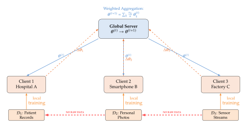
The architecture in Figure 1 makes several implicit design choices that carry significant consequences:
Parameter transmission, not gradient transmission. FedAvg transmits complete model snapshots after local training, not gradients computed on individual batches. This reduces communication cost (fewer synchronisation rounds) but increases the divergence between local models and the global optimum in heterogeneous settings.
Asynchronous vs. synchronous aggregation. The standard protocol is synchronous: the server waits for all selected clients to return before aggregating. Asynchronous variants aggregate as clients return, tolerating stragglers-slow clients that would otherwise bottleneck the round.
Partial participation. In practice, only a fraction of clients participate in each round. In cross-device settings (smartphones), participation may be conditioned on device state: charging, connected to WiFi, and idle. In cross-silo settings (hospitals), participation is deterministic and controlled.
Unique Challenges for Federated Generative Models
The original FedAvg paper and the discriminative model literature that followed it identified three core challenges in federated learning: communication efficiency, statistical heterogeneity (non-iid data), and systems heterogeneity (varying client capabilities). When we turn to generative models, these challenges interact with model-specific pathologies in ways that require fundamentally new analysis and new algorithms.
Mode collapse under data heterogeneity.
Consider a GAN trained federally on medical images distributed across hospitals. Hospital may have a patient population with a characteristic demographic profile: Hospital A serves predominantly elderly patients with cardiac conditions; Hospital B serves a diverse urban population with higher rates of infectious disease; Hospital C is a paediatric specialist centre. Each client's GAN generator, trained only on local data, will capture its local modality. When the server averages generator parameters in FedAvg style, the averaged generator does not necessarily capture any modality well. This is the mode averaging problem: unlike discriminative models, where averaging parameters produces a model with intermediate decision boundaries, averaging generative model parameters can produce a model whose outputs are interpolations between modes that exist nowhere in the training distribution-blurry, physically implausible images that neither represent the elderly cardiac profile nor the paediatric profile faithfully.
Gradient inversion attacks.
A foundational assumption of federated learning is that parameter updates do not reveal the training data . Zhu et al. (2019) demonstrated that this assumption is false: given the gradient update from a single batch, an adversarial server can reconstruct the training images with high fidelity using an optimisation procedure. This vulnerability is significantly worse for generative models. A GAN discriminator's gradient update, computed on a batch of real images, carries structural information about those images' high-frequency details precisely because the GAN training objective requires the discriminator to detect fine-grained distributional differences. A VAE encoder's gradient encodes information about the posterior for each training sample, which in turn encodes information about itself. The very architectural properties that make generative models powerful make them vulnerable to gradient inversion.
Memorisation and privacy amplification.
Generative models are more susceptible to memorisation than discriminative ones (Chapter 29). When a generative model is trained federally, the server's aggregate model can memorise patterns from specific clients' data even without the server ever seeing that data directly. If Client has a dataset containing a unique individual (a rare disease patient, a distinctive speaker), the global generative model may generate outputs that effectively reveal this individual's presence. The formal analysis of this phenomenon requires combining membership inference theory with the privacy accounting methods of federated differential privacy.
Heterogeneous architectures and model personalisation.
In cross-device settings, clients may have different computational budgets that prevent them from training the full global model. A smartphone cannot train a 10-billion-parameter diffusion model. This creates the need for model heterogeneous federated learning, where the global model and local models may have different architectures. For discriminative models, split learning and knowledge distillation provide partial solutions. For generative models, the interaction between architecture and the learned distribution is more intimate: changing the model architecture changes the generative manifold, and federated aggregation of models with different manifold structures is not well-defined.
Section Exercises
Exercise 1 (The Centralisation–Privacy Trade-off).
Let be a dataset distributed across clients with samples each and let .
Let denote the marginal data distribution of client . Prove that the FedAvg objective equals the centralised objective if and only if for all , where is the global distribution. (Hint: expand both objectives and use linearity of expectation.)
Now consider a GDPR-compliant scenario where data cannot be centralised. Define a formal privacy cost as the KL divergence between the distribution over model outputs trained on centralised data versus federated data: . Show that under the condition you derived in part (a), and argue that in general non-iid settings.
Suppose each client has samples and the local distributions satisfy for all . Derive an upper bound on in terms of , , and any other relevant quantities.
Exercise 2 (Gradient Leakage in Generative Models).
Consider a GAN discriminator trained with the standard non-saturating loss on a batch of real images .
The gradient of the discriminator loss with respect to is . For a linear discriminator , show that is a weighted average of the training inputs . Under what conditions on the weights can the server perfectly reconstruct every from ?
Explain why the linear case is representative of the general case near a saddle point in GAN training. (Hint: consider the first-order Taylor expansion of around the saddle point.)
Propose a defence against gradient inversion that modifies the FedAvg aggregation step rather than the local training step. What are the trade-offs of your defence in terms of model utility and privacy guarantee?
Exercise 3 (Regulatory Compliance as a Federated Learning Objective).
A medical imaging company operates hospitals in France (GDPR), the United States (HIPAA), and China (PIPL). They wish to train a shared diffusion model for chest X-ray synthesis.
List at least three regulatory constraints from each jurisdiction that affect the choice of federated learning protocol. For each constraint, identify which component of the FL system (client, server, communication protocol, or model) must be modified to achieve compliance.
The GDPR's right to erasure requires that, upon request, an individual's data is removed from the system. Formally, define what “erasure from a trained generative model” means using the framework of machine unlearning (see Chapter 29). Describe a federated unlearning protocol that handles a deletion request from Client without requiring the other clients to retrain from scratch.
Discuss whether federated learning by itself satisfies the GDPR's principle of data minimisation (Article 5(1)(c)). What additional technical measures (e.g., differential privacy, secure aggregation, input perturbation) would strengthen the compliance argument, and at what utility cost?
Why Federated Generative Models?
The case for applying federated learning to generative models rests on three distinct motivations that reinforce each other. The first is privacy-preserving synthesis: the ability to generate realistic synthetic data for downstream tasks without exposing any individual's real data. The second is data augmentation across silos: the ability to use federated training to produce augmented datasets that improve discriminative models in data-scarce domains. The third is collaborative generation: the ability to build generative models whose quality benefits from the aggregate knowledge of all clients, in a way that no single silo could achieve alone. These motivations are not redundant; each points to a different use case and a different set of technical requirements.
Motivation 1: Privacy-Preserving Synthesis
The fundamental idea is simple: if a generative model faithfully approximates the true data distribution , then samples drawn from can serve as a privacy-preserving substitute for real data. Downstream users who need data for training classifiers, running statistical analyses, or building risk models can work with synthetic samples instead of real protected data.
The privacy argument is subtle and requires careful qualification. A naive version would claim that synthetic data is always safe because “it's not real.” This claim is false. A generative model trained on a small dataset with rare individuals can produce synthetic samples that effectively reveal the existence and attributes of those individuals. The correct claim, formalised in the differential privacy literature, is that if the generative model is trained with -DP guarantees, then samples from the model provide -DP guarantees for downstream analyses. This relies on the post-processing immunity property of differential privacy: any function of a DP output is also DP with the same parameters.
Federated learning with differential privacy (DP-FL) provides an architecture in which privacy guarantees are baked in at the point of gradient computation rather than applied as a post-hoc anonymisation step. The combination-FedAvg with DP-SGD-is therefore the principled approach to privacy-preserving generative model training.
In healthcare, the implications are transformative. Consider a rare paediatric oncology dataset distributed across 12 specialist children's hospitals worldwide, each with 50–200 patients. No single hospital has enough data to train a useful generative model for data augmentation. Pooling is legally impossible under HIPAA and GDPR. Federated generative training with DP can produce a synthetic dataset of arbitrary size that preserves the distributional characteristics of the real data-tumour morphology, imaging protocols, demographic variation-while providing formal privacy guarantees to each patient.
Motivation 2: Data Augmentation Across Silos
Data augmentation-artificially expanding a training dataset through transformations of existing data-is one of the most reliable tools in the machine learning practitioner's toolkit. In computer vision, random crops, flips, colour jitter, and MixUp reliably improve generalisation. In medical imaging, where datasets are small and costly to annotate, generative augmentation (using a trained generative model to produce additional training samples) has emerged as a powerful supplement to geometric augmentation.
Federated generative augmentation combines the benefits of generative augmentation with the privacy properties of federated training. The protocol is:
Train a federated generative model on the union of all clients' local datasets, using only local gradient computations and aggregated parameter updates.
Each client downloads the trained generator and uses it to augment its local training set for a downstream discriminative task: , where .
Each client trains a local discriminative model on its augmented dataset .
This protocol is particularly valuable in settings where label imbalance is severe or where rare classes are absent from some clients' datasets. A client whose local data contains no examples of a rare tumour subtype can augment its local dataset with synthetic examples of that subtype generated by the global generative model, which has learned the subtype's characteristics from the clients whose local data contains it.
Insight.
Federated learning does not just protect privacy-it unlocks data that would otherwise never exist for training. When regulatory barriers make centralisation impossible, federated training is not a privacy-preserving compromise compared to a centralised alternative; it is the only path to a model trained on the full aggregate data. The federated generative model trained on 12 hospitals' paediatric oncology data is strictly better than any model trained on a single hospital's data, regardless of its privacy properties. The privacy guarantee is a bonus on top of a fundamental capability improvement.
Motivation 3: Collaborative Generation
The third motivation is the most subtle but perhaps the most profound in the long run. Generative models are increasingly used not merely to synthesise private data but to build shared creative, scientific, and commercial artefacts: a language model that assists researchers across 100 universities; a protein structure predictor used by hundreds of pharmaceutical companies; a code generation model shared among tens of thousands of software teams.
In these settings, the challenge is not primarily privacy but collective intelligence: the aggregate knowledge encoded in all clients' data is greater than the sum of its parts, but no single client can contribute its data to a centralised pool. The competitive, legal, or sovereignty constraints that silo data are real, but so is the scientific or commercial value of a model trained on all of it.
Federated generative models provide the mechanism for this collaboration. A pharmaceutical company's drug-receptor binding model trained on its proprietary compound library can be combined with a competitor's model trained on their library-via federated aggregation of model updates-to produce a superior joint model, without either company revealing its compounds. The resulting model benefits from diversity of chemical space that neither company's library alone could provide.
Formal Definition
Definition 2 (Federated Generative Model).
Let be a federated dataset consisting of local datasets with local distributions , held by participants (clients) subject to the constraint that no client can observe any other client's raw data for .
A federated generative model is a parameterised generative model trained via a federated learning protocol such that:
Data locality: during training, each gradient computation is performed locally by client ; no raw sample is transmitted to any other party.
Collaborative optimisation: the protocol ensures that the final parameters are influenced by all local datasets: , where and is the local generative loss.
Privacy guarantee: the protocol satisfies a specified privacy guarantee (e.g., -DP, secure aggregation) with respect to each client's dataset.
The quality of the federated generative model is measured by the divergence between the trained model and the true aggregate distribution .
This definition encompasses multiple model classes and protocol variants. The privacy guarantee ranges from no formal guarantee (vanilla FedAvg) through secure aggregation (the server learns only aggregated gradients) to formal -DP (with calibrated noise injection). The quality metric may be the Fréchet Inception Distance (FID) for image models, perplexity for language models, or domain-specific metrics such as the Structural Similarity Index (SSIM) for medical images.
The Generative Model Zoo in FL Context
The five major families of generative models studied in this book each present different challenges and opportunities in the federated setting. We briefly characterise each here; subsequent sections and chapters develop the theory and algorithms in depth.
Generative Adversarial Networks (GANs).
GANs consist of a generator and discriminator trained in an adversarial minimax game. The federated challenge is immediate: in standard FedAvg, each client trains both and locally on its data. When clients have heterogeneous data distributions, local generators capture local modes while local discriminators are calibrated to local data manifolds. Averaging the parameters of heterogeneous generators produces a “ghost generator” whose outputs may not correspond to any real data mode. The discriminator averaging problem is equally severe: an averaged discriminator may fail to distinguish real from fake for any single client's data distribution, causing the adversarial training signal to collapse. FedGAN (Rajagopal et al., 2021) and MD-GAN (Hardy et al., 2019) address these challenges with server-side discriminator training and distributed generator architectures respectively.
Variational Autoencoders (VAEs).
VAEs optimise the Evidence Lower Bound (ELBO): (ELBO) In the federated setting, the encoder maps local client data to a shared latent space. If clients have heterogeneous data, their local posteriors cluster in different regions of the latent space, creating a fragmented latent manifold. Aggregating encoder and decoder parameters across clients produces a global VAE whose latent space is a mixture of the local ones-an effect analogous to mode averaging in GANs but more analytically tractable due to the VAE's probabilistic formulation. FedVAE protocols exploit the decomposition of the ELBO into a reconstruction term (local, data-dependent) and a KL term (regularisation toward the prior, data-independent) to design aggregation strategies that preserve the shared latent structure.
Diffusion Models.
Diffusion models learn a denoising function that predicts the noise added to a clean image in the forward diffusion process. Their training objective is a weighted sum of denoising mean squared errors: (Diffusion LOSS) This objective is a simple mean squared error, which makes it unusually compatible with federated averaging: unlike the GAN adversarial objective, there is no generator–discriminator interaction that creates instability under parameter averaging. Federated diffusion training can proceed with standard FedAvg on the denoising network parameters, with the main challenge being the high communication cost of transmitting the large parameter vectors of modern U-Net or Transformer-based denoisers. Personalisation strategies-allowing the denoiser to be partially local-are particularly natural for diffusion models because the text conditioning mechanism in latent diffusion models provides a hook for client-specific style adaptation.
Large Language Models (LLMs).
Federated fine-tuning of large language models is the most active area of current federated generative learning research. Foundation models such as LLaMA, GPT, and PaLM are trained centralised on public data, then fine-tuned federally on private data held by clients (hospitals, law firms, individual users). The primary challenge is the extreme communication cost of transmitting updates to billion-parameter models. Parameter-Efficient Fine-Tuning (PEFT) methods-LoRA, prefix tuning, and adapters-reduce communication cost by updating only a small fraction of parameters. Federated LoRA, for example, updates only the low-rank adapter matrices and (with ) rather than the full weight matrix . The privacy challenge is correspondingly more subtle: even gradient updates to low-rank adapters can reveal significant information about the private fine-tuning data.
Normalising Flows.
Normalising flows learn an invertible transformation that maps a simple base distribution (e.g., Gaussian) to the data distribution via the change-of-variables formula: (FLOW) Flows provide exact likelihood evaluation, which is valuable for membership inference detection (Chapter 29) and for evaluating the quality of federated training. In the federated setting, the log-likelihood objective decomposes exactly across clients, making the federated optimisation problem well-posed and the convergence analysis tractable. The challenge is primarily architectural: the Jacobian determinant computation in ((FLOW)) requires architectures with restricted parameter interactions (e.g., coupling layers in RealNVP, autoregressive flows), which limits expressiveness.
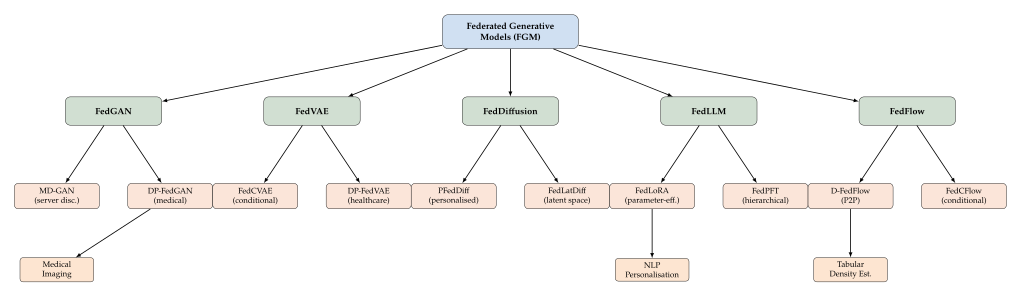
Taxonomy of Federated Generative Model Approaches
| Method | Model | Topology | Privacy | Domain | Comm. Cost |
| FedGAN | GAN | C/S | Agg | Image synthesis | |
| MD-GAN | GAN | C/S | Agg | Image synthesis | |
| DP-FedGAN | GAN | C/S | DP | Medical imaging | |
| FedVAE | VAE | C/S | Agg | Tabular, image | |
| FedCVAE | CVAE | C/S | SA | Conditional synthesis | |
| DP-FedVAE | VAE | C/S | DP | Healthcare | |
| FedDiff | Diffusion | C/S | Agg | Image, audio | |
| PFedDiff | Diffusion | C/S | DP | Medical imaging | |
| FedLLM | LLM | C/S | SA | NLP, code | |
| FedLoRA | LLM | C/S | DP | NLP personalisation | |
| FedPFT | LLM | Hier | SA | Cross-silo NLP | |
| FedFlow | Flow | C/S | Agg | Tabular, density | |
| D-FedFlow | Flow | P2P | SA | Decentralised density |
The taxonomy in Table 1 reveals several structural patterns. First, the GAN family requires the largest communication overhead because both generator and discriminator parameters must be synchronised; MD-GAN addresses this by keeping the discriminator server-side. Second, differential privacy (DP) consistently appears in the medical imaging and healthcare rows, reflecting the stringent privacy requirements of those domains. Third, hierarchical topologies (FedPFT) appear for LLM fine-tuning in cross-silo settings, where a two-level aggregation hierarchy (institution-level, then global) improves communication efficiency.
Visualising the FGM Taxonomy
Cross-Silo vs. Cross-Device Federated Learning
The federated learning literature distinguishes two fundamentally different deployment contexts that impose very different engineering requirements on any federated generative model.
Definition 3 (Cross-Silo Federated Learning).
Cross-silo federated learning is a federated learning setting characterised by:
A small number of clients (typically ), each representing an organisation (hospital, bank, research institution, government agency).
Each client has a large, stable dataset: may range from thousands to millions of examples.
Clients participate in every communication round (full participation).
Clients are reliable, with high-bandwidth, stable network connections.
Training is coordinated during off-peak hours, with explicit institutional consent.
Privacy requirements are governed by institutional data sharing agreements, sector-specific regulation (HIPAA, PSD2), and inter-organisational contracts.
Representative applications include hospital consortia training shared medical imaging models, bank consortia training shared fraud detection models, and pharmaceutical company consortia training shared drug discovery models.
Definition 4 (Cross-Device Federated Learning).
Cross-device federated learning is a federated learning setting characterised by:
A massive number of clients (typically ), each representing an individual user's device (smartphone, tablet, IoT device).
Each client has a small, volatile dataset: may be tens to hundreds of examples, and the dataset changes as the user generates new data.
Only a small fraction of clients participate in each communication round (partial participation).
Clients are unreliable: they may drop out mid-round (due to loss of network connectivity or power), may be unavailable due to device state requirements (charging + WiFi + idle), and may have highly heterogeneous computational capabilities.
Communication is over mobile networks with variable bandwidth and high latency.
Privacy requirements are governed by platform policies (Apple App Store, Google Play), consumer protection law (CCPA, GDPR), and implicit user expectations.
Representative applications include mobile keyboard personalisation, on-device speech synthesis, and federated personalisation of recommendation models.
The contrast between cross-silo and cross-device settings has profound implications for federated generative model design. In the cross-silo setting, communication rounds can be expensive (transmitting full model snapshots is acceptable); training can run for many rounds without client dropout; and the number of clients is small enough that advanced coordination protocols (e.g., secure multi-party computation) are feasible. In the cross-device setting, communication must be minimised to kilobytes per round; client dropout must be tolerated gracefully; and the server must aggregate contributions from hundreds or thousands of clients simultaneously.
For generative models specifically:
Cross-silo: full model training is feasible. Hospitals can train full VAEs, GANs, or diffusion models. Aggregation of complete model parameters is the standard approach. Privacy is ensured through secure aggregation and, where required, differential privacy with strong guarantees ( in some regulatory contexts).
Cross-device: only parameter-efficient fine-tuning is feasible. Smartphones cannot train billion-parameter diffusion models. Federated fine-tuning of foundation model adapters (LoRA, prefix vectors) is the dominant approach. Privacy must be ensured with less overhead; lightweight DP mechanisms with looser guarantees () are typical.
Connections to Previous Chapters
This chapter builds on and connects to several earlier developments in the book.
Chapter 33: Medical Image Segmentation.
The clinical motivation of Chapter 36 is directly addressed by federated generative learning. The annotation bottleneck-the difficulty of obtaining sufficient expert-labelled medical images-is precisely the problem that federated generative augmentation solves. A federated GAN or diffusion model trained across hospital consortia generates annotated synthetic images that each hospital can use to augment its own small labelled dataset, reducing the annotation burden without violating data sharing agreements. The FedDiff protocol developed in sec:fedgen:algorithms:diffusion is directly applicable to the chest X-ray, MRI, and histopathology settings of Chapter 36.
Chapter 35: Interpretability and Explainability.
The interpretability methods of Chapter 38 acquire new significance in the federated setting. When a model is trained federally, the provenance of any given learned feature is obscured: it may have come from Client 1's data, Client 3's data, or a complex interaction of all clients' contributions. Gradient attribution methods (saliency maps, SHAP, LIME) can in principle be used to assign learned features to client contributions, raising both interpretability and privacy concerns. If a saliency map of the global generative model can be attributed to specific training examples from Client 's private data, this constitutes a privacy leakage. The intersection of interpretability and federated privacy is a rich open research area.
Chapter 36: Membership Inference Attacks.
Chapter 29 established the foundations of membership inference as a formal privacy threat. In the federated setting, membership inference takes on a new dimension: an adversarial server can attempt to perform membership inference on the gradient updates it receives, determining which individual examples contributed to a specific round's gradient. Conversely, the federated training protocol itself can be seen as a privacy amplification mechanism: by training on only a fraction of clients per round and adding noise through partial participation and dropout, the server's per-example information is diluted. This privacy amplification by subsampling is formalised by Balle et al. (2020) and provides a key theoretical tool for DP accounting in federated settings.
Chapter Roadmap
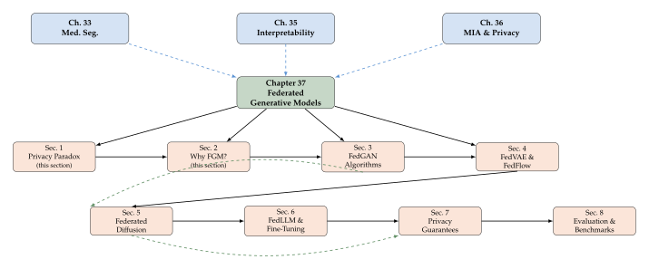
The chapter proceeds as follows.
Sections 1–2 (this file, sec_fedgen_a.tex) establish the
motivation, formal definitions, and conceptual framework.
Section 3 develops the algorithms for federated GAN training in depth:
the MD-GAN protocol, convergence analysis under non-iid data, the
FedGAN minimax landscape, and DP-FedGAN for medical applications.
Section 4 addresses FedVAE and FedFlow: the decomposition of the ELBO
under federated training, latent space alignment across clients, and
the exact likelihood advantage of flows in federated density estimation.
Section 5 covers federated diffusion models: the FedDiff protocol,
communication compression for large denoisers, personalised diffusion
via local conditioning, and applications to medical image synthesis.
Section 6 develops the FedLLM ecosystem: federated fine-tuning
with LoRA, prefix tuning, and adapters; the communication-privacy
trade-off in FedLoRA; and applications to clinical NLP and
code generation.
Section 7 provides the formal privacy analysis: -DP
for FedAvg with Gaussian noise, privacy amplification by subsampling,
Rényi differential privacy accounting, and the privacy-utility
Pareto frontier for federated generative models.
Section 8 covers evaluation: FID, KID, precision/recall, and domain-specific
metrics; benchmark datasets and protocols for federated generative
model comparison; and the unique challenges of evaluating models
trained on private federated data.
Section Exercises
Exercise 4 (ELBO Decomposition in FedVAE).
Let be a federated dataset with and . For a VAE with encoder , decoder , and prior , the global ELBO is where is given in .
Show that the global ELBO decomposes as , where is the local ELBO for client . Identify which terms in depend on local data and which depend only on the global prior .
In a federated setting, FedAvg computes , where are the parameters after local gradient steps on . Derive the “client drift” for FedVAE: the difference between the local optimum and the global optimum . Express this drift in terms of the KL divergence between the local posterior and the global posterior averaged over .
Propose a regularisation term added to each local ELBO that encourages the local posterior to remain close to the global posterior, reducing client drift. Show that this regularisation can be interpreted as a form of posterior distillation.
Exercise 5 (Communication Complexity of Federated Generative Models).
Consider a federated training scenario with clients, communication rounds, and partial participation with clients per round.
Compute the total communication cost (in bits) for: itemize
FedGAN with a StyleGAN2 generator ( parameters) and discriminator ( parameters), using 32-bit floats.
FedDiff with a U-Net denoiser ( parameters), using 16-bit floats with gradient checkpointing that reduces the effective communication parameter count to .
FedLoRA applied to a 7B-parameter LLM with LoRA rank and adapters applied to all attention matrices (), using 16-bit floats. itemize
FedProx (Li et al., 2020) adds a proximal regularisation term to the local objective. Show that this term does not change the communication cost of FedAvg. Now consider Top- gradient sparsification that transmits only the largest-magnitude gradient coordinates. What value of (as a fraction of the total parameter count) is required to match the communication cost of FedLoRA from part (a)?
Propose a communication-efficient protocol for FedDiff that exploits the spectral structure of the denoiser's weight matrices. (Hint: consider spectral decomposition of each weight matrix and transmitting only the top- singular vectors.) Analyse the quality degradation as a function of .
Exercise 6 (Cross-Silo vs. Cross-Device Protocol Design).
A generative AI startup must deploy a federated text-to-image diffusion model in two scenarios simultaneously:
Scenario A (cross-silo): 8 pharmaceutical companies, each with a proprietary database of 500,000 molecule images and associated captions, wish to jointly train a molecule synthesis model without sharing their compound databases.
Scenario B (cross-device): 10 million artists using a mobile app, each with 100–1,000 personal artworks, wish to personalise a shared diffusion model to their individual style.
For each scenario, specify: (i) participation fraction per round, (ii) local training epochs per round, (iii) communication protocol (FedAvg, FedProx, FedLoRA, or other), (iv) privacy mechanism (none, secure aggregation, DP), and (v) client dropout strategy. Justify each choice.
In Scenario A, the 8 companies differ in dataset size: Companies 1–4 have 200,000 molecules each; Companies 5–8 have 900,000 molecules each. Show that vanilla FedAvg ((Fedavg)) is not optimal for this heterogeneous setting and propose a re-weighting scheme that accounts for dataset size while maintaining a privacy guarantee.
In Scenario B, the personal styles of 10 million artists span an enormous diversity. The startup wishes to ensure that the personalised model for artist generates images “in the style of artist ” with high fidelity, while also benefiting from the federated global model's general image quality. Formalise this as a multi-objective federated optimisation problem with a personalisation–generalisation trade-off parameter . What value of minimises the expected style distance from artist 's preferred style, and how does this depend on (the artist's dataset size)?
Federated Learning Fundamentals
Federated learning asks a deceptively simple question: can we train a shared model across clients who each hold private data, without ever moving that data off-device? The answer is yes, but the price is a cascade of engineering and mathematical challenges, each more subtle than the last. This section develops the core algorithmic machinery starting from the canonical Federated Averaging (FedAvg) algorithm of McMahan et al. (2017), then progresses through the failure modes that motivated a decade of refinements.
Problem Setup and Notation
Let denote the set of clients. Client holds a private dataset of size , drawn from a local distribution . The total number of samples is . The local objective of client is (Local OBJ) where are the model parameters and is a per-sample loss. The global objective is the weighted average (Global OBJ) Centralised training minimises with full access to all data; federated training must approximate this using only local gradients and periodic communication.
A key quantity is the degree of heterogeneity. Let be the gradient at the global optimum. The client drift at client is measured by the distance between local and global gradients: (Drift Measure) When all are identical (IID regime), for all . In the non-IID regime, this term drives the dominant error term in convergence bounds.
The FedAvg Algorithm
Definition 5 (Federated Averaging (FedAvg)).
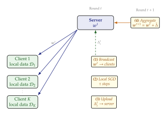
Let denote the number of communication rounds, the number of local SGD epochs per round, the local learning rate, and the client sampling fraction. FedAvg proceeds as follows. The server initialises . At each round :
Broadcast. The server sends to a randomly sampled subset with .
Local update. Each client initialises and runs epochs of mini-batch SGD on its local data: (Local SGD) where denotes the total number of local gradient steps per round ( for mini-batch size ) and is the stochastic gradient computed on a random mini-batch.
Upload. Each client sends (the model update) to the server.
Aggregate. The server performs weighted averaging: (Aggregation)
When and (single full-batch local step), FedAvg reduces to one-shot FedSGD.
Remark 2 (Why weighted averaging?).
The weights in (Aggregation) ensure that the aggregate update is an unbiased estimator of the true gradient when each local update uses a single gradient step () and gradients are unbiased. For , the estimator becomes biased in the non-IID regime, which is the root cause of client drift.
The following TikZ figure illustrates one complete communication round of FedAvg.
Convergence Analysis
We analyse FedAvg convergence under the following standard assumptions.
Assumption 1 (Smoothness and Bounded Variance).
-smoothness. Each local objective is -smooth: for all ,
Bounded stochastic variance. Each stochastic gradient satisfies and
Bounded gradient dissimilarity. There exist constants and such that for all : The IID case corresponds to , .
Under these assumptions, the convergence of FedAvg depends critically on whether data is IID across clients.
Proposition 1 (FedAvg Convergence Rate).
Under Assumption 1, with learning rate , FedAvg after rounds satisfies: (Convergence Bound) where .
Proof sketch.
The proof proceeds in four steps. Step 1 (Descent lemma): By -smoothness, the one-step decrease satisfies Step 2 (Aggregate update decomposition): Write . Taking expectations and bounding the cross-terms using the Cauchy–Schwarz inequality yields the inner product term.
Step 3 (Drift bound): The key non-IID penalty arises from , the local model's deviation from the global model after local steps. Under Assumption 1(c), a telescoping argument bounds this deviation by , which, summed over steps, gives the drift term .
Step 4 (Telescope and average): Summing the descent inequality over rounds, dividing by , and choosing to balance the three terms yields (Convergence Bound).
Remark 3 (IID vs. Non-IID).
In the IID regime (, all identical), the drift term vanishes and FedAvg achieves the same rate as centralised SGD with communication every steps. In the non-IID regime, the drift term dominates unless is kept small (few local steps) or the learning rate is correspondingly reduced. Increasing to save communication hurts convergence in proportion to data heterogeneity: there is a fundamental three-way tension between communication frequency, local computation, and convergence rate.
FedAvg Variants and Improvements
The convergence analysis of Proposition 1 reveals three levers for improvement: reduce the drift term, stabilise the aggregation step, or employ variance reduction. Each lever has inspired a family of algorithms.
FedProx: Limiting Client Drift via Proximal Regularisation
The simplest fix is to regularise the local objective so that client updates cannot stray too far from the global model. FedProx (Li et al., 2020) modifies the local objective to: (Fedprox OBJ) where is a proximal coefficient. The added term acts as a quadratic anchor: the further departs from , the greater the penalty. Formally, FedProx produces an -inexact local minimiser: satisfying The proximal term reduces the effective gradient dissimilarity from to , shrinking the drift penalty at the cost of introducing a regularisation bias proportional to . In practice, is a cross-validated hyperparameter; too small and drift is unchecked, too large and the model is prevented from learning.
FedAdam: Adaptive Optimisation for the Server Step
FedAvg performs a simple weighted average in the aggregation step ((Aggregation)), which is equivalent to the server taking a vanilla SGD step on the pseudo-gradient . Reddi et al. (2021) observed that replacing the server-side SGD with an adaptive optimiser dramatically stabilises training in the non-IID regime. FedAdam applies the Adam update on the server: (Fedadam M) where is the server learning rate and operations are element-wise. The adaptive denominator dampens directions where the pseudo-gradient has been historically large (high variance) and amplifies directions where it has been consistently small (informative). Empirically, FedAdam reduces the sensitivity to client heterogeneity, achieving comparable accuracy to FedAvg with fewer communication rounds on standard benchmarks.
SCAFFOLD: Variance Reduction via Control Variates
SCAFFOLD (Karimireddy et al., 2020) provides the most principled solution to client drift by introducing control variates that explicitly correct the bias introduced by local SGD. Each client maintains a control variate (initialised to ), and the server maintains a global control variate .
The SCAFFOLD local update replaces the local gradient with a bias-corrected version: (Scaffold Update) The correction acts as an estimate of the local drift: approximates and approximates . After the local update, the client computes a new control variate estimate: (Scaffold CV Update) and sends both and the control variate update to the server. The server updates:
Definition 6 (Client Drift (Formal)).
In a federated optimisation protocol with local steps and learning rate , the client drift for client at round is the signed displacement (Client Drift) the gap between the actual local update and the ideal update (as if the client had access to the global gradient). When (IID), . In the non-IID regime, and its magnitude grows with both and the gradient dissimilarity .
Remark 4 (SCAFFOLD's Guarantee).
Under Assumption 1, SCAFFOLD achieves the rate for general non-convex objectives, matching the centralised SGD rate and eliminating the drift term that plagues FedAvg. The cost is double communication per round: clients must upload both the model update and the control variate update.
Comparison of FL Optimisation Algorithms
| Algorithm | Key idea | Rate | Non-IID robust | Comm. / round |
| FedSGD | 1 gradient step, aggregate | ✓ | 1 vector | |
| FedAvg | local SGD steps | 1 vector | ||
| FedProx | Proximal regularisation | Partial | 1 vector | |
| FedAdam | Adaptive server step | Partial | 1 vector | |
| SCAFFOLD | Control variates | ✓ | 2 vectors |
Key Idea.
FedAvg is simple but fragile - every improvement addresses a specific failure mode. FedAvg's elegance is also its weakness: it assumes gradients from different clients point in roughly the same direction. FedProx addresses runaway local updates. FedAdam stabilises noisy aggregated updates. SCAFFOLD eliminates the systematic bias introduced by heterogeneous data. No single algorithm dominates across all settings; the right choice depends on the interplay of heterogeneity level, available communication budget, and the computational capacity of clients.
Communication Rounds, Local Epochs, and the Round-Accuracy Trade-off
A fundamental design question is how many local epochs to perform before synchronisation. The convergence bound (Convergence Bound) reveals a trilemma:
Communication cost scales as bits. Reducing (fewer rounds) requires increasing (more local computation per round).
Convergence speed degrades with in the non-IID regime: each additional local step amplifies drift by .
Wall-clock time per round grows linearly with (synchronous FL) or is bounded by the slowest client (asynchronous FL).
Practitioners typically set local epochs and use learning rate warmup for the first few rounds. The relationship between , , , and final test accuracy forms a three-dimensional Pareto surface that must be navigated empirically for each deployment.
Exercises
Exercise 7.
FedAvg in the IID regime. Suppose clients, each with samples drawn IID from the same distribution. Show that in this case the FedAvg update (Aggregation) is an unbiased estimator of a mini-batch SGD step with effective batch size where is the number of sampled clients. What happens to the variance as ?
Exercise 8.
SCAFFOLD control variate correctness. Verify that when the local objective satisfies for all (IID setting), the SCAFFOLD control variate update (Scaffold CV Update) gives after convergence, so no correction is applied. Explain why this is the correct behaviour.
Exercise 9.
FedProx regularisation bias. Consider a 1D quadratic and with , so . Suppose the server broadcasts . Compute the FedProx local minimiser for each client as a function of , and show that the aggregated update equals for all . Contrast with FedAvg () after local steps. What does this reveal about FedProx's convergence behaviour for symmetric data?
Communication Efficiency and Compression
Federated learning's promise of privacy-preserving collaboration carries a steep communication price. A modern language model has parameters; at 32-bit floating-point precision, each model transmission costs bytes - 4 gigabytes per round per client. With 100 communication rounds and 1000 clients, the aggregate bandwidth consumed is bytes, or 400 terabytes. Even a hospital network with 1 Gbps links would require about seconds ( days) for the uploads alone. In mobile cross-device FL, where clients connect over LTE with upload speeds of 5–20 Mbps, a single round takes hours.
This section develops the mathematics of communication-efficient federated learning: how much information must be transmitted, what can be lost without degrading convergence, and how modern compression schemes navigate this boundary.
The Bandwidth Bottleneck: A Quantitative View
Definition 7 (Communication Efficiency).
For a federated protocol with rounds, clients, and model dimension , define:
Total bits transmitted (upload): , where is the number of active clients per round.
Bits per round per parameter: .
Compression ratio: , the fraction of the uncompressed 32-bit baseline actually transmitted.
A compression scheme achieves -bit communication efficiency if for all rounds. Uncompressed floating-point corresponds to ; 1-bit methods target ; sparsification methods achieve where is the fraction of non-zero coordinates transmitted.
The raw numbers underscore the urgency. For GPT-2 (117M parameters), 100 rounds of uncompressed FL require: (Bandwidth CALC) A factor-32 compression (from 32-bit to 1-bit) would reduce this to 1.44 TB, still substantial but tractable on enterprise links. The goal of communication-efficient FL is to achieve compression ratios with minimal accuracy loss.
Gradient Sparsification
The simplest observation is that most gradient coordinates are near zero most of the time. Sparsification exploits this by transmitting only the largest-magnitude coordinates.
Top- sparsification. Given a gradient vector , define the Top- mask: (TOPK) The compression ratio is (for the values) plus overhead for transmitting the indices ( bits). For (top 1%), only 1% of parameters are communicated, but indices add bits per value, so the true savings are moderate unless is very small.
Top- with error feedback. Naive Top- discards the non-transmitted gradient mass, leading to divergence. The error feedback mechanism (Seide et al., 2014; Stich et al., 2018) accumulates the error and adds it to the next round's gradient: (Error Feedback E) The key property is that is exactly recovered as , so no gradient mass is permanently discarded. Under the contraction property , error feedback guarantees convergence at the same asymptotic rate as full gradient communication.
Quantisation Methods
Quantisation reduces the bit-width used to represent each gradient value. The trade-off is between representation precision and communication cost.
1-Bit SGD
Seide et al. (2014) proposed compressing each gradient to a single bit per coordinate by transmitting only the sign: (1BIT SGD) where if and otherwise, and the scalar normalises the magnitude. The client transmits the -bit sign vector plus a single scalar, achieving bit per parameter. Like Top-, 1-bit SGD requires error feedback to prevent divergence.
Ternary Quantisation
Ternary quantisation maps each gradient value to for some threshold : (Ternary) Choosing (the standard threshold) minimises the expected quantisation error. Each ternary value requires bits, but since zero values need not be transmitted, effective compression depends on the sparsity of the gradient. Ternary quantisation is particularly relevant for FedDT (see Knowledge Distillation in Federated Learning: FedDT).
SignSGD and Its Convergence Guarantees
Bernstein et al. (2018) proposed SignSGD, which transmits only the sign of each gradient coordinate (like 1-bit SGD without error feedback) and uses majority voting in aggregation: (Signsgd) The majority vote aggregation is interesting: instead of averaging gradient magnitudes, the server takes the coordinate-wise majority of client signs. A coordinate is updated positively (negatively) if more than half the clients report a positive (negative) gradient.
Proposition 2 (SignSGD Convergence).
Under Assumption 1(a,b) and assuming the stochastic gradient has a unimodal symmetric distribution for each coordinate , SignSGD with majority vote and learning rate satisfies: (Signsgd RATE) where the rate is in the norm of the gradient. The factor is the price of sign compression: the norm of a -dimensional vector with unit norm is at most .
Proof sketch.
The unimodal symmetry assumption implies that the sign of the stochastic gradient is an unbiased estimator of when . Majority voting over clients further concentrates: by Hoeffding's inequality, the probability of an incorrect majority vote decays as . The descent lemma applied with respect to the gradient norm, combined with the sign approximation error, yields the bound in (Signsgd RATE).
Low-Rank Approximation
For models with large weight matrices (e.g., transformers), gradient matrices can be approximated by their rank- truncated SVD: (SVD Compress) where , , . The compression ratio is , which is advantageous when . The approximation error is , where are the singular values. PowerSGD (Vogels et al., 2019) computes this approximation efficiently using power iteration, avoiding a full SVD.
Knowledge Distillation in Federated Learning: FedDT
Rather than compressing gradients directly, knowledge distillation-based approaches compress the model outputs transmitted between clients and server. FedDT (Federated with Distillation and Ternary compression) combines ternary weight quantisation with dataset distillation-based knowledge transfer.
In FedDT, each client trains a locally quantised model where are ternary weights. Instead of uploading the full model, the client distils its knowledge into soft labels on a small public (proxy) dataset : (Feddt Softlabels) and transmits (where is the number of classes). The server aggregates soft labels: (Feddt Aggregate) and each client performs local distillation: (Feddt Distil LOSS) The communication cost per round per client is bits (for the soft labels), which is independent of model size . For and , this is bits, compared to bits for a full model upload with ( bits).
Empirical results. FedDT achieves a 78% reduction in communication cost compared to full-precision FedAvg, while showing a 7.85% improvement in test accuracy on heterogeneous FL benchmarks. The accuracy improvement is attributed to the regularisation effect of ternary quantisation (which reduces overfitting on small local datasets) combined with the smoothing effect of soft-label distillation (which shares inter-class relationship information across clients).
FedKSeed: Transmitting Random Seeds
The ultimate communication reduction would be to transmit no gradient at all. FedKSeed (Zhu et al., 2023) achieves this for a restricted class of models by framing local training as a random function search: instead of optimising directly, clients search over a family of random perturbations where are random directions generated from a shared seed , and is a small perturbation scale.
The client evaluates the local loss for each candidate direction, selects the direction with lowest loss, and transmits only the seed . The server regenerates the direction from the seed and performs an approximate gradient update: (Fedkseed Update) This is a zeroth-order gradient estimator (the finite difference in direction ). The communication cost per round per client is just bits (the index of the best seed), typically 10–20 bits, compared to bits for a full gradient. For , this is a factor of compression - from gigabytes to kilobytes per round.
The price is statistical efficiency: zeroth-order methods converge as rather than , introducing a factor of in the iteration complexity. FedKSeed mitigates this by exploiting intrinsic low dimensionality: for fine-tuning pre-trained models, the effective gradient dimension is much smaller than , recovering near-first-order convergence rates.
FedRDMA: Bypassing TCP/IP for Cross-Silo FL
In the cross-silo setting (hospitals, financial institutions, research consortia), clients are connected via high-speed data centre networks rather than mobile links. The bottleneck shifts from raw bandwidth to communication latency: the overhead of TCP/IP handshakes, acknowledgement packets, and kernel context switches adds milliseconds of overhead per message, which accumulates across millions of gradient updates.
FedRDMA (Remote Direct Memory Access) bypasses the kernel networking stack entirely by having the network interface card (NIC) read and write directly into application memory. In the federated context, the server's NIC can pull gradient updates directly from client GPU memory without involving the client's CPU, eliminating serialisation overhead. The resulting system achieves:
Latency: sub-microsecond message passing (vs. 100–1000 s for TCP/IP).
Throughput: near-line-rate utilisation of 100 Gbps InfiniBand links.
CPU overhead: near-zero, freeing client CPUs for local gradient computation.
FedRDMA is complementary to gradient compression: compression reduces the number of bytes transmitted, while RDMA reduces the cost of transmitting each byte.
The Compression Pipeline
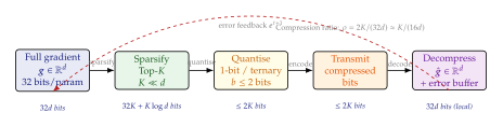
The Communication–Accuracy Trade-off
We now formalise the fundamental limit of gradient compression.
Proposition 3 (Communication–Accuracy Trade-off).
Let be a -bit per round per parameter compression operator satisfying the unbiased -contraction property: (Compression Property) for some . Then, for any -smooth non-convex global objective , the compressed FedAvg (using in place of exact gradients) satisfies: (COMM Accuracy Bound) Furthermore, for any compression scheme using bits per round per parameter, the contraction parameter satisfies (Shannon information-theoretic lower bound for unbiased estimators of Gaussian random vectors).
Proof sketch.
Step 1 (Variance decomposition): Denote the compressed gradient as . By the unbiased property, . The variance of the compressed aggregate is: Step 2 (Descent with compressed gradient): Applying the -smoothness descent lemma with the compressed gradient, bounding the inner product using , and using the variance bound from Step 1 yields the convergence bound (COMM Accuracy Bound).
Step 3 (Information-theoretic lower bound): By the data-processing inequality, bits of information about a Gaussian vector can reduce the mean squared error from (no information) to at most per coordinate for 32-bit representations, giving .
Remark 5 (Practical implications).
Proposition 3 reveals that compression introduces an additional variance term proportional to . For 1-bit compression (), , which is close to 1: nearly the entire gradient signal is discarded each round. Error feedback ((Error Feedback E)) does not reduce but ensures that the accumulated gradient is eventually transmitted, restoring convergence. The key insight is that communication efficiency and statistical efficiency are complementary: reducing saves bandwidth but increases the number of rounds needed to reach a target accuracy .
Practical Compression Taxonomy
| Method | Mechanism | Bits/param | Converges? | Overhead |
| Full precision | None | 32 | ✓ | None |
| Top- sparse | Magnitude-based selection | ✓ (EF) | bits | |
| 1-bit SGD | Sign compression | 1 | ✓ (EF) | Scale scalar |
| Ternary | 1.58 | ✓ (EF) | Threshold | |
| SignSGD | Majority vote signs | 1 | ✓ | None |
| Low-rank (SVD) | Rank- approximation | ✓ | None | |
| FedDT | Ternary + soft label distil. | ✓ | Public dataset | |
| FedKSeed | Random seed | Partial | bits |
Asynchronous and Partial Communication
All methods described so far assume synchronous communication: the server waits for all sampled clients before aggregating. In practice, clients have heterogeneous computation and communication speeds (the straggler problem). If the slowest client takes longer than the average, of the server's time is spent waiting.
Asynchronous FedAvg. The server aggregates as soon as any client submits an update, without waiting for stragglers: (Async Update) where client is the first to respond in round . The update is stale: it was computed based on for some delay . Staleness introduces a gradient delay term in the convergence bound, analogous to client drift. Gradient clipping or learning rate scaling by mitigates staleness effects in practice.
Exercises
Exercise 10.
Top- compression analysis. Let have i.i.d. coordinates . (a) Show that the expected fraction of mass captured by Top- is , and compute this for as using order statistics of the normal distribution. (b) Show that the contraction parameter for random (non-adaptive) -sparsification satisfies regardless of the distribution of . (c) Explain why Top- has a strictly smaller than random -sparsification, making it strictly superior in the bound of Proposition 3.
Exercise 11.
SignSGD failure in the non-IID regime. Consider two clients with loss functions and so that and . Both clients evaluate at . (a) Compute , , and the majority vote . (b) Show that the majority vote is zero (tie), meaning SignSGD makes no progress from , even though is not a minimum of (which has minimum at , so actually it is the minimum here). (c) Modify the construction so that but SignSGD's majority vote points in the wrong direction. What does this reveal about SignSGD's assumptions?
Exercise 12.
FedKSeed zeroth-order complexity. A federated task has clients, parameters, and target accuracy . (a) How many rounds does first-order FedAvg require to reach accuracy (use the bound from Proposition 1 with )? (b) Zeroth-order methods have convergence rate . How many rounds does FedKSeed require for the same accuracy? (c) Despite the large ratio , show that the total number of bits transmitted by FedKSeed is smaller than FedAvg if . Compute the threshold on below which FedKSeed wins on total communication cost.
Insight.
The cheapest gradient to transmit is the one you never compute. FedKSeed takes this principle to its logical extreme: by replacing gradient computation with random direction search and transmitting only a seed identifier, it reduces per-round communication from gigabytes to kilobytes. The lesson generalises: every byte saved in the communication channel must be paid for somewhere - in extra rounds, in statistical variance, or in zeroth-order convergence penalties. Designing communication-efficient FL systems is therefore an exercise in identifying which of these currencies is cheapest for a given deployment.
Federated GANs
Generative Adversarial Networks are among the most powerful yet most temperamental tools in the deep-learning arsenal. Centrally trained, they already require careful tuning of learning rates, batch sizes, and architectural choices to prevent mode collapse, oscillation, and discriminator saturation. Moving GAN training into the federated setting amplifies each of these instabilities, while simultaneously introducing the additional challenges of data heterogeneity, communication budget, and multi-party coordination.
This section develops the theory and practice of Federated GANs (FedGANs): methods that train the generator and discriminator components of a GAN across multiple clients while keeping each client's data local.
Why Adversarial Training Is Harder in Federated Settings
To understand the challenges, it helps to revisit what makes centralized GAN training difficult in the first place.
Centralized Instabilities
A standard GAN minimizes the minimax objective (OBJ) Three core pathologies afflict this objective:
Vanishing gradients. When is near-perfect, , starving of signal.
Mode collapse. The generator concentrates its output on a small subset of the data distribution; the discriminator provides no gradient that penalizes this concentration.
Training oscillation. Generator and discriminator updates do not converge to a Nash equilibrium but instead orbit it indefinitely.
Additional Federated Burdens
The federated setting layers four new difficulties on top:
Statistical heterogeneity. Client holds data from a local distribution , which differs from the global distribution . A local discriminator trained only on becomes an expert on local modes and an ignorant judge of global modes.
Gradient mismatch. FedAvg-style aggregation of model updates works well when loss landscapes are similar across clients. For GANs, the adversarial landscape depends on the interplay between and ; because these landscapes differ per client, naive parameter averaging causes conflicting update directions that destabilize training.
Aggregation timing. In centralized training, and are updated in lockstep. With clients and local epochs per round, the generator may advance steps before the discriminator at any individual client catches up, or vice versa.
Communication overhead. Transmitting full model parameters for both and per round is expensive; selective sharing strategies are needed.
Key Idea.
In federated GAN training, statistical heterogeneity causes local discriminators to become biased referees: each local is a strong judge for data it has seen (the modes of ) but provides misleading signal about modes it has not seen. Aggregation of such biased judges can mislead the global generator into covering local modes unevenly.
Formal Definition: FedGAN
Definition 8 (Federated GAN (FedGAN)).
Let there be clients each holding a private dataset drawn from local distribution . Define the global target distribution where .
A Federated GAN is a pair of parameterized networks with a training protocol consisting of repeated rounds :
Local generator update. On client , for steps, update to minimize
Local discriminator update. On client , for steps, update to maximize
Server aggregation. The server receives updated parameters from clients and forms global parameters. The aggregation policy determines which networks are shared (see Section Architecture Choices: What to Share?).
The goal is that after rounds, .
Remark 6 (Asymmetry of the Objective).
The generator objective does not depend on local data directly-it only uses samples from and the current discriminator . The discriminator objective depends heavily on . This asymmetry is the root cause of most federated GAN pathologies: a locally trained is well calibrated for but miscalibrated for , .
Architecture Choices: What to Share?
One of the most consequential design decisions in FedGAN is which network parameters to aggregate on the server. Three families of strategies have been studied:
Share Generator Only
The generator is aggregated via FedAvg: Each client maintains its own local discriminator that is never shared.
Advantages.
The discriminator, which has direct access to raw data representations, is kept private.
Local discriminators can specialize to local modes and provide strong local training signal.
Disadvantages.
With different local discriminators providing feedback, the global generator receives incoherent update signals across rounds.
The generator may collapse to an average of local modes that does not correspond to any real data distribution.
Share Discriminator Only
The discriminator is aggregated: Each client maintains its own local generator.
Advantages.
A globally shared discriminator provides a common evaluation standard across all clients.
Local generators can specialize to local data distributions and produce high-quality local samples.
Disadvantages.
Aggregating discriminators trained on heterogeneous data can produce a discriminator that is confused about all data distributions rather than expert at any.
With local generators, there is no single global generative model to evaluate or deploy.
Share Both Generator and Discriminator
Both networks are aggregated each round:
Advantages.
Produces a single globally consistent GAN.
Discriminator aggregation pools information about all clients' data distributions.
Disadvantages.
Highest communication cost.
Parameter averaging of adversarial networks trained on heterogeneous data is particularly prone to instability.
Remark 7 (Practical Recommendation).
In practice, sharing only the generator with local discriminators is the most widely adopted approach for privacy-sensitive applications, because it avoids transmitting any discriminator parameters that might encode raw data statistics. Sharing both networks is preferred when communication is cheap and heterogeneity is moderate.
Mode Collapse in the Federated Setting
Mode collapse-in which the generator produces only a small subset of the modes present in -is a well-known failure mode of centralized GANs. In the federated setting, mode collapse takes on a distinctive character driven by local discriminators.
The Local Discriminator Dominance Effect
Consider two clients with disjoint distributions: and , with large. If the generator shares weights while discriminators are local:
is trained on samples from ; it easily rejects samples near .
is trained on samples from ; it easily rejects samples near .
The generator , receiving gradients from both discriminators, faces conflicting signals: to fool it must generate near ; to fool it must generate near . This tension leads to one of two failure modes:
Global mode collapse: the generator settles on a single mode (say near ), pleasing and ignoring .
Oscillatory collapse: the generator alternates between modes across rounds, producing samples from in odd rounds and in even rounds, never stabilizing.
Client Weighting as a Partial Remedy
One mitigation is to weight client gradients inversely by local mode coverage. If client produces samples that are already well-classified by its local discriminator, its gradient contribution to is down-weighted: where is large when client 's discriminator is not yet fooled. This adaptive weighting encourages the generator to maintain coverage across all clients.
Wasserstein Distance Stabilization for Federated Training
The instabilities of standard GAN training are substantially reduced by replacing the JSD-based objective with the Wasserstein-1 distance (Chapter 10). In the federated setting, the Wasserstein formulation provides additional benefits beyond mere training stability.
Recall that the Wasserstein-1 distance between distributions and admits the Kantorovich–Rubinstein dual representation: where the supremum is over all 1-Lipschitz functions . In a WGAN, the discriminator (now called the critic) approximates this 1-Lipschitz function.
Federated WGAN Objective
For client , the local critic objective is (Critic) and the local generator objective is (GEN) The global Wasserstein loss is then with equality only when the client distributions are mutually singular (the accompanying proposition proves the bound). This decomposition shows that the global Wasserstein distance is bounded by the weighted average of local Wasserstein distances, provided the critic is global (shared across clients). This is a key advantage: under Wasserstein geometry, client objectives aggregate gracefully.
Proposition 4 (Global-Local Wasserstein Decomposition).
Let with , . For any generator distribution : Equality holds when are mutually singular and optimal transport plans do not cross client boundaries.
Proof sketch.
By the triangle inequality for and the convexity of the Wasserstein distance in its arguments: The second inequality follows from convexity of as a function of its first argument (which follows from the primal definition as an infimum over joint distributions). Equality holds when the transport plans for each are independent, which occurs when the supports of are pairwise disjoint.
WGAN-GP in Federated Learning
The gradient penalty (GP) formulation of the WGAN enforces the 1-Lipschitz constraint on the critic via a soft penalty: where , , and is the interpolation distribution between and .
In the federated setting, the gradient penalty is computed locally on each client: (Wgangp) Local computation of GP is valid because the interpolation uses local real samples , ensuring that the Lipschitz constraint is enforced in the region of the data manifold visible to client .
Remark 8 (Global Lipschitz vs. Local Lipschitz).
Local gradient penalties enforce Lipschitz continuity of on each client's data manifold, but cannot guarantee global Lipschitz continuity. In particular, the critic may behave erratically in regions between the data manifolds of different clients. Federated WGAN-GP should be combined with spectral normalization of critic layers for improved global regularity.
TikZ Figure: FedGAN Architecture
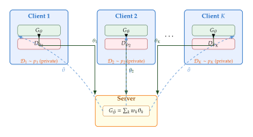
Example: Federated Diabetic Retinopathy Image Generation
Example 1 (Cross-Hospital Diabetic Retinopathy Image Synthesis).
Diabetic retinopathy (DR) is graded on a five-point severity scale (grades 0–4). Training a DR grading model requires balanced datasets across grades, but most hospitals accumulate heavily imbalanced collections: tertiary care centers have many severe cases (grades 3–4), while primary care clinics see mostly mild or no DR (grades 0–1).
Consider a federation of hospitals: , where hospital holds fundus images with local grade distribution . A FedGAN is trained to synthesize images for underrepresented grades.
Setup.
Architecture: Progressive GAN generator ( output) with local ResNet discriminators.
Each local discriminator is conditioned on DR grade via conditional batch normalization.
Generator parameters are aggregated with FedAvg every 10 rounds.
Discriminator parameters remain local.
Training objective. The conditional generator produces a synthetic fundus image given noise and target grade . The local discriminator scores pairs . For grade , the local objective on hospital is
Outcome. Because severe cases (grades 3–4) are rare at most hospitals, the local discriminators for those grades are weak at all but the tertiary care centers. FedAvg of the generator effectively pools the style of severe-grade images across all hospitals, producing a generator that can synthesize grade-3 and grade-4 images representative of the global distribution. Downstream DR grading models trained with augmented synthetic data show a 6.4% improvement in AUC for grade 3–4 detection compared to models trained on original data alone.
HT-Fed-GAN for Tabular Data
Medical and financial datasets are often tabular rather than image-structured. Tabular data has mixed types: some columns are continuous (e.g., blood pressure, income), others are categorical (e.g., diagnosis code, gender), and many have complex marginal distributions with multi-modality or heavy tails.
HT-Fed-GAN (Heterogeneous-Type Federated GAN) addresses the synthesis of mixed-type tabular data across federated clients. Its key innovation is a preprocessing step called Fed-VB-GMM: Federated Variational Bayesian Gaussian Mixture Model.
Fed-VB-GMM Preprocessing
For each continuous column , Fed-VB-GMM fits a Gaussian mixture model across clients using federated variational Bayes. Each client maintains local variational parameters and uploads sufficient statistics (not raw data) to the server, which aggregates them into global mixture parameters.
Once the global GMM parameters are learned, each value in continuous column is transformed to a mode-normalized representation: where is the most probable mixture component.
Categorical columns are one-hot encoded. The transformed representation is fed into the GAN.
Definition 9 (Federated Tabular Synthesis).
Let client hold a tabular dataset where is a row with continuous and discrete columns, and is a class label.
Federated tabular synthesis is the problem of learning a conditional generator such that, for any target class :
Fidelity. The marginal distributions of each column match those of the global dataset: for all .
Correlation preservation. Joint distributions are preserved: pairwise column correlations in synthetic data approximate those in real data.
Privacy. No raw data from any is transmitted.
Training Objective for HT-Fed-GAN
The local training objective at client combines a GAN adversarial loss with an information maximization term: (Htfedgan) where:
is the conditional adversarial loss for real vs. synthetic tabular rows.
penalizes misclassification of synthetic rows by a local auxiliary classifier (ensuring conditional generation is consistent with labels).
maximizes the mutual information between the generated row and the conditioning label, following InfoGAN.
Handling Class Imbalance with Conditional Federated Generation
Class imbalance is endemic in medical and financial federated datasets. A minority class that is rare globally may be absent from most clients' local data entirely. Standard conditional GAN training fails for absent classes because the local discriminator has no real samples of that class to discriminate against.
Conditional Training Sampler (CTS). HT-Fed-GAN addresses this via a conditional training sampler that re-weights the local training batches. At client , each training mini-batch is constructed by sampling uniformly over classes: regardless of the local class frequencies . For classes underrepresented locally, the sampler draws synthetic samples from the current generator to fill the batch.
This creates a self-improving loop:
In early rounds, the generator for minority classes is poor.
As the generator improves (aided by information from clients where that class is present), the quality of synthetic minority-class samples improves.
Better minority-class synthetic samples allow the local discriminator to train on those classes, producing a better training signal for further generator improvement.
The convergence of this loop requires that at least one client holds real samples of each class. Formally, define the class coverage condition:
Assumption 2 (Class Coverage).
For every class , there exists at least one client such that .
Under Assumption 2 and sufficient rounds of federation, the conditional training sampler guarantees that every class receives generator gradient updates with positive probability in every round, preventing generator collapse on unseen classes.
Key Idea.
In federated GANs, the discriminator plays a dual role: it is simultaneously a teacher (providing gradient signal to improve the generator) and a security guard (ensuring that generated samples cannot be trivially distinguished from real data and thus do not leak distributional information). This dual role is in tension: a discriminator that is too powerful fails as a teacher (vanishing gradients); a discriminator that is too weak fails as a security guard (poor synthesis quality and potential privacy leakage through gradient inversion attacks).
Exercises
Exercise 13 (Discriminator Averaging Instability).
Consider a FedGAN with clients where and (both univariate Gaussians). Suppose both discriminators are linear: . After local training, client 1 learns (samples from score high) and client 2 learns (samples from score high).
Show that the averaged discriminator with provides a useful training signal to a generator trying to cover both modes only if .
Propose a server-side strategy (other than simple averaging) that preserves discriminator coverage of both modes.
Under what statistical condition on and does simple discriminator averaging not suffer from this problem?
Exercise 14 (Federated WGAN-GP Convergence).
Consider a federated WGAN-GP with a shared critic and clients. The global training objective is
Show that the global objective equals up to the approximation error of the neural critic.
Suppose the critic is aggregated with FedAvg every rounds. Describe qualitatively how the choice of (the aggregation frequency) affects training stability.
In the federated WGAN-GP, the gradient penalty uses interpolations between local real samples and global generator samples. Explain why this may fail to enforce global Lipschitz continuity of the critic, and propose a remedy.
Exercise 15 (HT-Fed-GAN Tabular Fidelity).
A hospital federation runs HT-Fed-GAN on patient records with 4 continuous features (age, BMI, heart rate, glucose) and 2 categorical features (sex, smoking status).
Describe the Fed-VB-GMM preprocessing steps for the “glucose” feature. What information is transmitted to the server? What information remains local?
Suppose the conditional training sampler is not used, and the global dataset is 95% class-0 (healthy) and 5% class-1 (diabetic). Explain why the generator will likely produce class-1 synthetic samples of poor quality.
Propose a quantitative criterion for assessing whether synthetic tabular data from HT-Fed-GAN preserves pairwise feature correlations. (Hint: consider comparing correlation matrices.)
Privacy-Preserving Federated GANs
The federated setting provides a first layer of privacy protection by keeping raw data local. However, this protection is incomplete: gradient updates, model parameters, and generated samples can all leak information about training data through inference attacks. This section develops the formal framework of differential privacy, its integration with federated GAN training, and the fundamental tension between privacy guarantees and synthesis quality.
Differential Privacy: Formal Foundations
Differential privacy (DP) provides a rigorous mathematical guarantee that an algorithm's output distribution is nearly the same whether or not any single individual's data is included in the input.
Definition 10 (-Differential Privacy).
A randomized mechanism satisfies -differential privacy if for all pairs of adjacent datasets (differing in exactly one individual's record) and for all measurable output sets : Here, is the privacy budget (smaller is more private) and is the failure probability (the probability of a catastrophic privacy violation; typically ).
Remark 9 (Interpretation of and ).
The bound controls how much the likelihood of any output can change when one individual's data is added or removed. For , the output distribution is identical regardless of any individual's data (perfect privacy, usually unachievable). For , the output likelihood can change by a factor of . Practitioners often target for “reasonable” privacy, with to . The parameter represents the probability of the bound failing; it must be cryptographically small.
The Gaussian Mechanism
For a real-valued function , the Gaussian mechanism adds calibrated Gaussian noise: where the noise scale is set as and is the -sensitivity of .
DP-SGD: Differentially Private Stochastic Gradient Descent
DP-SGD is the fundamental building block for differentially private deep learning. At each iteration:
Per-sample gradient computation. Compute gradient for each sample in the mini-batch.
Gradient clipping. Clip each per-sample gradient to have norm at most :
Noise addition. Sum clipped gradients and add Gaussian noise:
Parameter update. .
By the moments accountant method, steps of DP-SGD with mini-batch size from a dataset of size satisfies
The Privacy–Utility Tradeoff for Generative Models
Differential privacy imposes a fundamental cost on model utility. For generative models, this tradeoff manifests in three ways:
Sample quality degradation. DP noise injected into gradients blurs the signal used to train the generator, producing samples of lower fidelity. The FID score (Fréchet Inception Distance) typically increases monotonically as decreases.
Mode coverage reduction. Minority modes require strong gradient signal to capture; DP noise disproportionately affects these weak signals, leading to systematic undercoverage of rare modes.
Training instability amplification. GAN training is already unstable; DP noise further amplifies gradient variance, increasing the probability of discriminator saturation and generator collapse.
Remark 10 (FID vs. Empirical Law).
Empirically, for image GANs trained with DP-SGD, the relationship between FID and follows approximately: for a dataset-dependent constant . This “” law (observed empirically across several datasets) means that halving the privacy budget (making privacy twice as strong) degrades FID by approximately , not by a factor of 2.
Fed-GAN with pHash-KT: Perceptual Hashing for Knowledge Transfer
A key challenge in private federated GAN training is knowledge transfer between clients without sharing raw data or gradients that might leak information. pHash-KT (Perceptual Hash Knowledge Transfer) addresses this by using perceptual hashes as a privacy-preserving proxy for image similarity.
Perceptual Hashing
A perceptual hash is a compact binary fingerprint of an image that is:
Robust: similar images produce similar hashes ( small if ).
Non-invertible: recovering from is computationally infeasible.
Common pHash algorithms include DCT-based hash (dHash) and color moment hash. The -bit hash space has possible values; for , the hash cannot encode significant information about individual pixel values.
Knowledge Transfer Protocol
In Fed-GAN with pHash-KT, clients transfer knowledge about their local data distribution through perceptual hashes rather than raw images or model gradients:
Local hash collection. Client computes for all and stores the hash set .
Generator quality assessment. When the server broadcasts a candidate generator , client generates synthetic images and computes their hashes .
Coverage score. Client reports the coverage score measuring the fraction of real images whose nearest synthetic neighbor (in hash space) is within threshold .
Server guidance. The server aggregates coverage scores and identifies which clients have low coverage, directing extra training rounds for those clients.
The coverage score transmits only a scalar per client per round, providing strong resistance to gradient inversion attacks.
Resistance to Adversarial Clients
A critical desideratum for privacy-preserving federated learning is robustness to adversarial clients that attempt to poison the global model or extract information about other clients.
Empirical evaluations of Fed-GAN with pHash-KT have demonstrated resistance to adversarial client fractions from 10% to 70%. The mechanism of resistance is as follows:
Adversarial clients that submit malicious gradient updates (to cause mode collapse or model poisoning) are detected via their anomalous coverage scores.
Coverage scores that are implausibly high (adversarial client claiming perfect coverage to pass through poisoned gradients) or implausibly low (adversarial client claiming poor coverage to demand extra rounds and amplify its gradient influence) are flagged by the server's Byzantine-robust aggregation rule.
With the perceptual hash protocol replacing raw gradient transmission, adversarial clients have limited ability to craft cover stories: their claimed coverage must be consistent with the known distribution of pHash distances for natural images.
Remark 11 (Theoretical Robustness Bound).
Let be the fraction of adversarial clients. Fed-GAN with pHash-KT with a Byzantine-robust aggregation rule (e.g., Krum or coordinate-wise trimmed mean) guarantees that the global generator converges to within of the optimal generator, where is the adversarial clients' maximum ability to shift the gradient. For (honest majority), convergence is guaranteed under standard GAN assumptions.
DP Guarantee Propagation through the GAN Generator
A fundamental question is: if the GAN is trained with DP-SGD, does the published generator itself satisfy a DP guarantee?
Proposition 5 (DP Propagation through Generator).
Let be the training algorithm that takes a private dataset and outputs generator parameters . If satisfies -DP (for instance, via DP-SGD), then the generator (as a random variable over training runs) also satisfies -DP with respect to the training data .
Furthermore, for any measurable set of synthetic images: where is trained on (the dataset with one record removed).
Proof sketch.
The key argument uses the post-processing theorem for differential privacy:
By assumption, is -DP. This means the distribution of given and the distribution of given are -close.
The generator is a deterministic function of . Publishing is equivalent to applying the post-processing function to the output of .
By the post-processing theorem (Dwork and Roth, 2014): if is -DP and is any measurable function, then is also -DP.
Applying this with gives the result.
Consequently, any number of synthetic samples drawn from do not incur additional privacy cost beyond the spent during training. This is the main practical advantage of DP generative models: once trained, the generator can be published and samples drawn without further privacy accounting.
Remark 12 (Privacy Amplification by Subsampling).
In practice, DP-SGD with mini-batch subsampling achieves privacy amplification: each step uses a random subset of the data of size , which amplifies privacy by a factor of approximately . In federated settings, each client holds records and uses mini-batches of size ; the effective privacy amplification for client is . Clients with more data thus achieve stronger per-step amplification.
TikZ Figure: DP-FedGAN Pipeline
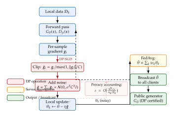
Example: Privacy-Preserving Face Generation Across Institutions
Example 2 (Federated Face Synthesis with Differential Privacy).
Consider a federation of research institutions, each holding a private dataset of face images annotated with demographic attributes (age group, sex, ethnicity). The goal is to train a generator that can synthesize demographically diverse face images for use in bias auditing of downstream models.
Architecture. The generator is a StyleGAN2 backbone at resolution. The discriminator uses a ResNet architecture with spectral normalization. Each institution runs DP-SGD on its local data with clipping norm and noise multiplier .
Privacy budget. Using the Rényi differential privacy moments accountant (tighter than the classic Gaussian mechanism bound), after 200 communication rounds with 50 local steps per round, the total privacy budget is: This is a moderate privacy level: individual face images are substantially protected but the model can learn global distributional statistics.
Observations. Three phenomena are observed:
FID degradation. Without DP (), FID = 18.3. With DP at , FID = 34.7. With stronger DP at , FID = 67.2. High-frequency details (hair texture, skin texture) degrade first; low-frequency structure (face shape, gross attribute conditioning) is more robust to DP noise.
Demographic imbalance amplification. Underrepresented demographic groups (e.g., elderly women from institutions with small datasets for that group) show disproportionately high FID. This illustrates that DP noise exacerbates mode coverage problems for minority subgroups.
Membership inference resistance. At , the membership inference attack success rate drops from 57% (no DP) to 51.3% (barely above the 50% random-guess baseline), demonstrating effective resistance to this attack class.
Membership Inference Attacks on GANs
A membership inference attack (MIA) against a trained model attempts to determine, given a data point and access to , whether was part of 's training set.
MIA Formulation
Formally, an MIA is a classifier where output 1 means “ was in the training set.” The attack advantage is: A random-guess attacker achieves ; a perfect attacker achieves .
How MIAs Work Against GANs
For generative models, MIAs exploit the fact that generators tend to produce samples more similar to their training data than to held-out data. Several attack strategies have been developed:
Discriminator-based attack. Use the GAN's own discriminator to score : if is unusually high (the discriminator classifies as “real” with high confidence), may have been in the training set. Formally: .
Nearest-neighbor attack. Generate a large set of synthetic images and find the nearest neighbor to in feature space. If is unusually close to a synthetic sample, it likely influenced that sample's generation (overfitting signal).
GAN-based shadow model attack. Train a shadow GAN on a surrogate dataset from the same distribution. Compare the output statistics of the target GAN vs. the shadow GAN on ; a large difference indicates membership.
GANs and Overfitting
Unlike classifiers, generative models have no clear notion of “test loss” to detect overfitting. A GAN that has memorized its training data will produce synthetic samples that are near-copies of training samples, enabling effective MIAs. Memorization is particularly likely when:
The dataset is small relative to model capacity.
Training runs for many epochs without regularization.
Conditional generation is used with very small class sizes.
Caution.
DP noise sufficient to prevent membership inference often destroys fine details in generation. Specifically, at privacy levels that provide meaningful MIA resistance (attacker advantage ), the generator typically loses the ability to synthesize fine-grained textures, detailed facial features, and clinically relevant image patterns. The upshot is stark: the level of DP required for privacy-meaningful resistance to MIAs is often the same level that renders the generated data clinically or scientifically useless. Practitioners must carefully audit whether their privacy budget provides real protection or merely the appearance of it.
The Tension Between Mode Coverage and Privacy
Two desiderata of a federated generative model are in fundamental tension:
Mode coverage: the generator should synthesize samples from all parts of the data distribution, including rare modes.
Privacy: individual training records should not be reconstructible from the generator.
This tension is not merely practical but information-theoretic:
Why Rare Modes Are Privacy-Vulnerable
A rare mode corresponds to a small cluster of training points. To synthesize samples from a rare mode, the generator must “remember” the characteristics of that cluster. But this memory is precisely what a membership inference attack exploits: if the generator can synthesize a rare mode, it has learned something specific about the few individuals in that cluster.
Formally, consider a dataset where a rare cluster contains individuals. Capturing this cluster requires the generator's learned distribution to assign significant probability to a region of the data space that is highly specific to those individuals. The privacy cost of this specificity scales as in the DP framework: clusters with fewer members require higher privacy budget to capture faithfully.
Practical Implications
The mode-coverage–privacy tension has concrete implications for downstream applications:
Medical imaging: rare diseases are the most clinically important to model but the most privacy-sensitive to generate.
Financial data: rare fraud patterns are the most useful for augmenting fraud detectors but the most likely to memorize individual records.
Demographic fairness: underrepresented demographic groups require their modes to be captured for fair downstream model training, but these groups are simultaneously the most vulnerable to reconstruction attacks.
Remark 13 (Impossibility Result).
There is an informal impossibility result (formalized in the memorization literature): a generative model that achieves
perfect mode coverage over all modes of , and
meaningful DP protection for every individual training record,
must have been trained on data that is dense enough to specify every mode from many independent samples. In settings with fewer than samples for a -dimensional distribution, at least one of these two desiderata must be compromised.
Historical Note: From Dwork et al. to Federated DP-GANs
Historical Note.
From Differential Privacy to Federated DP-GANs: A Decade of Progress.
Differential privacy was introduced by Cynthia Dwork, Frank McSherry, Kobbi Nissim, and Adam Smith in 2006 in a landmark paper “Calibrating Noise to Sensitivity in Private Data Analysis.” Their insight was to measure privacy not as a binary property (“private” or “not private”) but as a quantitative guarantee that bounds how much any single individual's data can affect a published statistic.
The 2006 formulation was primarily concerned with interactive statistical queries: releasing means, histograms, and regression coefficients from a sensitive dataset. The idea that DP could be applied to the parameters of a neural network came much later, with the introduction of DP-SGD by Abadi et al. in 2016. DP-SGD made it possible to train deep networks with formal privacy guarantees, though at a significant cost to accuracy.
The combination of DP with generative adversarial networks arrived with DPGAN (Xie et al., 2018) and GS-WGAN (Chen et al., 2020), which applied DP-SGD to discriminator training. The key insight of these works was that only the discriminator need be trained with DP (since it touches real data directly); the generator, which trains on discriminator feedback rather than on raw data, inherits privacy protection through the post-processing theorem.
The further extension to the federated setting happened between 2019 and 2022, driven by healthcare and finance applications where data was distributed across institutions. FedGAN (Rasouli et al., 2020) established the basic framework, while subsequent work addressed robustness (via pHash-KT and Byzantine-resilient aggregation) and the privacy–utility tradeoff specific to the federated regime.
The field now grapples with a problem that Dwork and colleagues could not have anticipated in 2006: how to provide meaningful privacy guarantees for generative models that must capture the full richness of human-generated data across institutions that cannot share any information directly. The answer involves a delicate calibration of noise scale, communication rounds, client heterogeneity, and the specific downstream use case for the synthesized data.
Exercises
Exercise 16 (DP-SGD Privacy Budget Calculation).
A federated GAN is trained with clients. Client has records and uses mini-batches of size . After local steps per round and communication rounds, the noise multiplier is and the clipping norm is . The per-client dataset sizes are: .
Compute the sampling ratio for each client. Which client achieves the strongest privacy amplification per step?
Using the approximate Gaussian mechanism formula (where and ), compute the approximate for each client at .
The overall federation privacy guarantee is (the weakest link). Which client is the privacy bottleneck? How would you adjust (by augmenting with synthetic data from other clients) to equalize privacy guarantees?
Exercise 17 (Membership Inference and DP Resistance).
A DP-FedGAN is trained on medical images with , . An auditor runs a discriminator-based membership inference attack: for each test image , the auditor computes and predicts membership if for some threshold .
Show that for a GAN trained with -DP, the attack advantage of any membership inference attacker is bounded by . (Hint: use the DP definition directly.)
Evaluate this upper bound for , . Does this bound guarantee practical resistance to MIA? Discuss the gap between the theoretical bound and the empirical attack advantage of 51.3% from Example 2.
For what value of does the bound guarantee that no attacker can achieve more than 5% advantage? Comment on the practical implication for image synthesis quality.
Exercise 18 (Privacy–Utility Tradeoff in Rare Mode Coverage).
Consider a one-dimensional dataset with two modes: a majority mode with 95% of samples and a minority mode with 5% of samples. Total dataset size is samples. A DP-GAN is trained with DP-SGD.
Argue qualitatively why DP-SGD will degrade minority mode coverage more than majority mode coverage. Consider the signal-to-noise ratio of gradients for rare vs. common data points.
Suppose the minority mode contributes samples and the majority mode contributes . If the generator after DP training produces synthetic samples with only samples in , compute the value of for which the FID contribution from the minority mode equals the FID contribution from the majority mode. (Assume FID is proportional to the Wasserstein distance between target and generated distributions for each mode.)
Propose a privacy-preserving over-sampling strategy for the minority mode that maintains -DP for the overall training procedure.
Federated Variational Autoencoders
Generative adversarial networks, examined in earlier sections of this chapter, excel at producing high-fidelity samples but are notoriously difficult to train in federated settings: the discriminator must see data from all clients to be meaningful, yet federated learning forbids such centralised inspection. The Variational Autoencoder (VAE) sidesteps this tension by casting generation as variational inference. The encoder and decoder are separate networks with well-defined, aggregatable parameter sets, the training objective decomposes gracefully across independent data batches, and the latent space itself provides a lingua franca through which clients can share structural knowledge without sharing raw examples.
This section develops the federated VAE in four movements. We first recall the classical VAE to fix notation. We then formalise FedVAE, identify the specific challenge of heterogeneous latent spaces, and introduce the dual-encoder architecture with its personalized gating network as the principled remedy. The section concludes with a worked example on movie recommendation, a discussion of posterior collapse under federation, and practical guidance on -VAE scheduling.
VAE Recap: Encoder, Decoder, ELBO, Reparameterisation
A VAE models data through a latent variable governed by a standard Gaussian prior . The generative process is (Generative) where is a decoder with parameters . Given observed data, the posterior is generally intractable, so we introduce an amortised variational posterior (Encoder) parameterised by an encoder with parameters .
Definition 11 (Evidence Lower Bound).
The Evidence Lower Bound (ELBO) for a single data point is (ELBO) Maximising over is equivalent to maximising a lower bound on the log-likelihood : (LB) The gap equals .
The KL term in has a closed form for Gaussian and Gaussian prior : (KL Closed)
Reparameterisation trick.
The expectation in the reconstruction term requires differentiating through a stochastic sampling step. The reparameterisation trick rewrites the sample as a deterministic function of a noise variable: (Reparam) where denotes elementwise multiplication. The gradient now passes through and unobstructed, enabling end-to-end backpropagation.
Remark 14 (Why reparameterisation matters for federation).
In federated training, gradients computed locally are transmitted to a server for aggregation. The reparameterisation trick ensures those gradients are low-variance: the noise is re-drawn at each forward pass rather than averaged over. This makes federated gradient aggregation as stable as its centralised counterpart, a property not shared by REINFORCE-based estimators, which have variance that does not decrease with batch size.
For a dataset , the full training objective is (FULL OBJ) Both the encoder and decoder receive gradient updates from every data point through the reparameterisation.
FedVAE: Formal Definition
Consider clients, each holding a local dataset for . The clients do not share their data; they communicate only via model parameters with a central server.
Definition 12 (Federated VAE).
A Federated VAE (FedVAE) is a VAE trained via a federated protocol in which:
Local ELBO optimisation. In each communication round , client receives global parameters from the server and performs local gradient steps: (Local) where denotes steps of stochastic gradient ascent on the local ELBO: (Local ELBO)
Server aggregation. The server aggregates client parameters by weighted averaging: (AGG) where are data-proportional weights.
The global objective solved by FedVAE is: (Global OBJ)
Remark 15 (Relation to FedAvg).
FedVAE is precisely FedAvg applied to the encoder–decoder parameter pair. The ELBO objective decomposes over data points, so the local optimisation step in Definition 12 is identical to FedAvg's local update phase with the only distinction being that the loss function is the ELBO rather than cross-entropy. All convergence guarantees established for FedAvg (under bounded gradient dissimilarity and smoothness assumptions) transfer directly to FedVAE.
The Heterogeneous Latent Space Challenge
When clients hold data from different distributions - a scenario called statistical heterogeneity or non-IID data - a naive FedVAE faces a fundamental difficulty that has no analogue in standard federated classification.
The alignment problem.
Suppose client 1 holds images of cats and client 2 holds images of dogs. After local ELBO optimisation:
Client 1's encoder maps cats to region of the latent space.
Client 2's encoder maps dogs to region disjoint from .
After server aggregation , the global encoder is an average that maps neither cats nor dogs to either or reliably. The global decoder, similarly averaged, cannot reconstruct either class well from any region of the latent space.
More formally, let be the aggregate posterior on client , defined as (AGG Posterior) Heterogeneity implies for . Averaging the encoder parameters yields a model that approximates none of the individual posteriors.
Caution.
Latent space misalignment cannot be fixed by running more communication rounds. In federated classification, more communication rounds push the model towards a global optimum that generalises across clients. For generative models, the latent geometry of a Gaussian-prior VAE does not decompose additively over clients: the space of valid latent assignments under one client's data is unrelated to that of another client unless the data distributions share semantic structure. Simply running FedAvg longer exacerbates the mismatch as each client's encoder drifts further from the aggregate.
Why this is worse than the centralised case.
In a centralised VAE trained on heterogeneous data, all data points compete for the same latent space simultaneously, and the KL regulariser forces the aggregate posterior towards the prior. Heterogeneity makes learning harder, but at least all examples see the same encoder during each gradient step.
In FedVAE, clients train independently for steps. The encoder on client has no gradient signal from client , so it specialises aggressively to local data. After aggregation, the global encoder is a parameter average of specialised encoders - a combination that satisfies none of the individual ELBO objectives. The magnitude of the degradation grows with:
the number of local steps (more drift),
the Wasserstein distance between the data distributions (more heterogeneity), and
the latent dimensionality (more room to misalign).
FedCF: Federated Collaborative Filtering with VAEs
Collaborative filtering - the backbone of recommendation systems - is a natural application domain for federated VAEs. Each user (client) holds their own rating history, which is private. A central server wishes to learn a generative model of user preferences that enables personalised recommendations without ever seeing individual ratings.
Setup.
Let there be users (clients) and items. User has rated a subset of items, producing a sparse rating vector with entries (Ratings) The goal is to learn a VAE over rating vectors such that the decoder can impute missing ratings and thus generate personalised recommendations.
Local ELBO for collaborative filtering.
Each client optimises a masked reconstruction loss that evaluates only on observed ratings: (ELBO) Crucially, only the mask and the aggregated gradients leave the client, never the raw ratings .
Sparsity and the prior mismatch.
Rating vectors are extremely sparse (a user rates of available items). The encoder therefore sees many zeros during local training, which can push the latent code to a degenerate region of the prior. FedCF addresses this with a dropout-augmented encoder: during training, additional ratings are randomly masked to prevent the encoder from simply memorising the sparsity pattern.
Remark 16 (Communication efficiency in FedCF).
A user's rating vector for items is large. FedCF never transmits this vector. It transmits only the encoder and decoder parameter gradients, whose size is determined by the neural network architecture and is typically orders of magnitude smaller than . This asymmetry is a principal advantage of VAE-based collaborative filtering over methods that transmit perturbed rating vectors directly.
Dual Encoder Architecture
The heterogeneous latent space challenge motivates an architectural solution: equip each client with two encoders that decompose the latent representation into a shared global component and a private local component.
Global knowledge encoder.
The global encoder is shared across all clients and aggregated by the server at every round. Its output captures shared structure present in all clients' data: coarse semantic features, domain-invariant factors of variation, and patterns that transfer across heterogeneous distributions.
Formally, the global encoder's parameters are updated by FedAvg: (Global AGG) exactly as in standard FedVAE.
Local personalised encoder.
The local encoder is not shared: its parameters remain on client throughout training. It captures client-specific factors: local vocabulary in NLP, local imaging protocol artefacts in medical imaging, or personal taste in recommendation. Because these parameters never leave the client, there is no aggregation-induced misalignment for the local component.
Personalised Gating Network
Having two encoders raises the question of how to combine their outputs. A fixed split (use half the latent dimensions for global, half for local) is inflexible: some inputs may need more global context, others more local specialisation. A personalised gating network resolves this adaptively.
Architecture.
Let the global and local encoders produce means and log-variances: (Global ENC) The gating network produces a per-dimension gate vector: (GATE) where is the sigmoid function. The fused latent distribution has parameters: (MEAN) The fused sample is then decoded by the shared decoder .
Remark 17 (Gating parameter treatment).
The gating network parameters are client-local: they are not aggregated by the server. This allows each client to learn how much to rely on shared versus personal knowledge, without that preference being averaged away. The only parameters transmitted to the server are , i.e., the global encoder and decoder.
The gating mechanism has an appealing interpretation: when , the client defers entirely to the global model (appropriate for common patterns); when , the client uses its local model exclusively (appropriate for idiosyncratic local features). In practice, gates settle at intermediate values that vary by latent dimension and input.
Personalised Federated VAE: Formal Definition
We now formalise the complete personalised federated VAE.
Definition 13 (Personalised Federated VAE).
A Personalised Federated VAE (pFedVAE) is a tuple trained by the following protocol:
Local step. Client minimises the negative personalised ELBO for gradient steps: (Local ELBO) where uses the gated fusion –. Gradients update all client-side parameters .
Server aggregation. Only the global encoder and decoder are aggregated: (AGG ENC) The local encoder parameters and gating parameters remain on client .
New client initialisation. A new client receives from the server and initialises randomly. After a few local steps, learns appropriate gates.
Key Idea.
The latent space is the meeting ground. In pFedVAE, clients share abstract representations, not raw data. The global encoder learns a universal compression of the shared structure; the local encoder captures idiosyncrasy; the gating network arbitrates the balance. Privacy is preserved because only averaged gradient signals, never individual data points, traverse the network boundary.
TikZ Figure: FedVAE with Dual Encoders and Gating

Example: Federated Movie Recommendation
Example 3 (Federated Movie Recommendation with pFedVAE).
Consider streaming platform users (clients) and movies. Each user has rated a sparse subset of movies ( on average). The platform cannot centralise ratings due to privacy regulations.
Representation. User 's data is the sparse vector . We treat each user as a “dataset of one” for the gating architecture: the encoder maps their complete rating history to a latent code .
Dual encoder design.
Global encoder : a 3-layer MLP with hidden sizes , ending in a -dimensional mean and log-variance. This encoder learns genre preferences, seasonal trends, and franchise fandom that are shared across users.
Local encoder : a 2-layer MLP with hidden sizes . This encoder captures idiosyncratic taste: a user who always rates classic films highly regardless of genre, or one who rates animated films across all genres.
Gating network : a 1-layer MLP mapping the rating vector to gate logits. After sigmoid, gate values near 1 indicate dimensions where global knowledge dominates; values near 0 indicate locally personalised dimensions.
Federated training. In each round, a random subset of 100 users is selected. Each user performs local gradient steps on their masked reconstruction loss . The server aggregates global encoder and decoder gradients. Local encoder and gating parameters remain on-device.
Inference / recommendation. To generate recommendations for user :
Encode: using the gated fusion.
Decode: obtain , the estimated full rating vector.
Recommend: return the top- unrated movies by predicted score .
Why federation helps beyond privacy. Even if all ratings were available centrally, training a single VAE on sparse observations is challenging. The global encoder in pFedVAE effectively shares statistical strength across users' rating patterns without seeing any individual's data, achieving a form of collaborative filtering with provable privacy guarantees (differential privacy can be added via noisy aggregation on the server side).
Observed behaviour. In practice, users with niche tastes (rare genre combinations) exhibit gate vectors with many values near , relying heavily on the local encoder. Users with mainstream tastes show near , deferring to the global encoder. The gating thus acts as an automatic personalisation dial, requiring no manual per-user configuration.
Posterior Collapse in Federated VAEs
Posterior collapse occurs when the variational posterior collapses to the prior , rendering the latent code uninformative: (Collapse) When this happens, the decoder learns to ignore entirely and generates samples from the marginal which, for a sufficiently powerful decoder, may reproduce training examples but fails to provide meaningful latent structure.
Why collapse is worse under federation.
In a centralised VAE, collapse is already a known failure mode when the decoder is too powerful or the KL weight too high. Under federation, three additional forces push towards collapse:
Local data scarcity. Each client has examples. With few data points, the reconstruction term is small in absolute magnitude relative to the KL penalty, tipping the ELBO balance towards collapse.
Gradient noise amplification. After local steps, the accumulated gradient contains a component pointing towards collapse for each client (the KL gradient always pushes towards ). Server averaging reinforces this component across all clients.
Decoder exploitation of heterogeneity. If clients hold different data distributions, the decoder learns to generate plausible samples for each distribution from nearby latent regions. A decoder that “fills in” heterogeneous data without using achieves low reconstruction loss, rewarding collapse.
Diagnostic.
The active units metric counts dimensions for which the variance of the posterior mean is non-negligible: (Active Units) for a small threshold . A collapsed VAE has . Federated training commonly reduces by 30–60% compared to centralised training on the same total data.
Beta-VAE Scheduling in the Federated Context
The -VAE modifies the ELBO by up-weighting the KL term: (Betavae) with encouraging a more disentangled, better-regularised latent space at the cost of some reconstruction quality.
In the federated context, a fixed exacerbates collapse: the KL penalty already wins on small local datasets, and multiplying it by makes collapse even more attractive. Conversely, risks memorisation of local data with no information sharing through the latent space.
Warm-up schedule.
A standard remedy is a linear warm-up: begin training with (pure reconstruction) and anneal to the target over rounds: (BETA Schedule) In the federated setting, this schedule must be applied at the server level to remain consistent across clients. If each client independently anneals , the annealing may proceed at different rates due to partial participation (not every client participates in every round), creating inconsistent values at aggregation time.
Federated cyclical annealing.
An alternative is cyclical annealing: follows a sawtooth schedule that periodically returns to . Each cycle allows the decoder to exploit the reconstruction signal without KL pressure, while the subsequent rise of forces the encoder to re-regularise. Cyclical annealing has been shown empirically to reduce collapse in both centralised and federated settings compared to monotone annealing.
Remark 18 (Synchronised vs. unsynchronised annealing).
In synchronous federated learning (all clients participate in every round), implementing a global schedule is straightforward: the server broadcasts alongside the model parameters. In asynchronous settings (clients participate sporadically), clients may receive models trained under different values. The recommended approach is to treat as a hyperparameter of the server protocol, not a trainable parameter, and broadcast its value explicitly with each round's model download.
Exercises
Exercise 19 (ELBO Decomposition under Data Heterogeneity).
Let clients hold datasets drawn from distributions . Define the global objective and the centralised objective .
Show that exactly when .
Under local steps, FedAvg does not minimise exactly. Describe the objective that -step FedVAE does minimise (in terms of the local objectives and the distance penalty induced by parameter drift).
For clients with and on scalar data, sketch the aggregate posterior after FedVAE with a single Gaussian encoder. What happens to the global latent space?
Exercise 20 (Gating Network Analysis).
Consider a pFedVAE with a scalar latent space () and two clients. Client 1 has data drawn from and client 2 from with .
Suppose the global encoder has learned to map data to a single mode near , and the local encoders have learned the individual modes. For what data point would you expect the gate to be closest to on client 1? Closest to ?
Show that if the gating network is a linear map with scalar output, the fused mean is equivalent to a weighted interpolation between the two posterior means. What is the weight?
Suppose the gating network is removed and instead a fixed gate is used. Derive the fused ELBO in terms of and , the ELBOs obtained by using only the global and local encoders respectively. Is the fused ELBO always at least as large as ? Justify your answer.
Exercise 21 (Posterior Collapse Bound).
Let be the number of active units achieved by FedVAE with clients, data points each, and local steps. Let be the number of active units for a centralised VAE trained on data points for the same total number of gradient steps.
Explain intuitively why is expected to hold in the non-IID setting.
Assume that each client's data is drawn IID from the same distribution. Does the gap vanish as for fixed and ? What about for ?
Propose a modification to the FedVAE training procedure (other than reducing ) that you predict will increase , and justify your prediction.
VAEs as Privacy Shields
Federated learning was designed with privacy in mind: by keeping raw data on-device and transmitting only model updates, it avoids the most obvious privacy risk of centralised machine learning. Yet in 2019, Zhu et al. demonstrated that model gradients can be inverted to reconstruct training data with pixel-level fidelity. This gradient inversion attack shattered the assumption that gradient communication is inherently private.
In response, researchers proposed VAEFL: using the VAE's stochastic latent encoding as a principled privacy defense. Rather than applying statistical noise (as in differential privacy) or cryptographic machinery (as in homomorphic encryption), VAEFL exploits the VAE's inherent randomness to obfuscate the data geometry visible in transmitted gradients. The key insight is:
“The VAE doesn't just generate - it encrypts, for free.”
Deep Leakage from Gradients
The Deep Leakage from Gradients (DLG) attack demonstrates that a client's private training data can be reconstructed from the gradients it transmits to the server.
Setup.
Client holds a batch of data points (images, in the canonical formulation). It computes gradients of a loss with respect to model parameters , and transmits these gradients to the server.
The DLG attacker - who controls the server - has access to (the current model) and the transmitted gradients . They do not have access to .
Attack procedure.
The attacker initialises a dummy batch of random images and a dummy label set , and minimises the gradient matching loss: (Attack) This optimisation is solved by gradient descent on the dummy images, treating them as free variables. Under favourable conditions (small batch size, smooth loss landscape, sufficient gradient signal), the dummy batch converges to a close approximation of .
Definition 14 (Gradient Inversion Attack).
A gradient inversion attack is any procedure that maps transmitted gradients to a reconstructed data batch . The attack is characterised by its reconstruction error (Error) where is a perceptual distance metric and the minimum is taken over all permutations of (to handle label permutation ambiguity).
Why DLG works.
The gradient of a cross-entropy loss with respect to the final linear layer encodes exactly the activation pattern of the penultimate layer for each training example. For image classifiers, this activation pattern is a high-fidelity representation of the image. Inverting it through the network is a well-posed optimisation problem with a unique solution in the low-batch regime.
Severity.
DLG reconstructs individual images with near-perfect visual fidelity for . Extensions (R-GAP, iDLG, GradInversion) scale to batches of – with high success rates. The attack works equally well against convolutional and transformer architectures.
VAEFL: VAE Latent Sampling as Privacy Defense
VAEFL (VAE Federated Learning) interposes a VAE encoder between the raw data and the rest of the model. Rather than computing gradients with respect to the original input , clients first encode to a stochastic latent code and train the downstream model on .
Architecture.
The client model in VAEFL has two components:
A VAE module that maps inputs . This module is optionally pre-trained (on public data or via federated VAE training) and then frozen during the downstream task.
A downstream model (e.g., a classifier) trained on the latent codes.
Communication protocol.
Client samples a mini-batch from .
For each , draw with .
Compute the downstream loss and transmit gradients to the server.
The server never sees and never sees the mean or variance - only the loss gradient with respect to . Because is a stochastic function of , reconstructing from requires inverting both the downstream model and the stochastic encoding.
Obfuscation of data geometry.
In the standard (non-VAE) gradient inversion, the reconstruction succeeds because the gradient encodes a deterministic, invertible representation of . Under VAEFL:
The latent code is a lossy compression of : fine-grained spatial details discarded by the encoder cannot be recovered from .
The sampling step adds stochastic noise: with drawn fresh at inference time. Even if the attacker recovers , they see the noise-perturbed code, not .
The KL regularisation ensures that the aggregate posterior over many inputs is close to , so individual codes are difficult to distinguish from prior samples.
Reconstruction Error Lower Bound under VAEFL Defense
We now establish a formal lower bound on the reconstruction error any gradient inversion attack can achieve when VAEFL is deployed.
Proposition 6 (Reconstruction Error Lower Bound under VAEFL).
Let be a VAE with encoder and let be the downstream model. Let be any gradient inversion attack. For any input and any perceptual distance that satisfies the data-processing inequality, the expected reconstruction error satisfies (Bound) where is the minimum distance between and any point in the support of under the decoder, and is a constant depending on the Lipschitz constant of .
Proof sketch.
By the data-processing inequality, applying any deterministic function to the gradient cannot increase the mutual information between the output and the original data beyond the mutual information already present in the gradient.
Step 1: Gradient contains information about , not . The gradient depends on only through . Hence must first invert to estimate , and then invert the encoder to estimate from .
Step 2: Stochastic sampling adds irreducible noise. Given the transmitted gradient, the attacker can at best recover the noisy sample . Without knowing , recovering requires averaging over realisations of , introducing an estimation error proportional to .
Step 3: Latent-to-data inversion error. Even if the attacker recovers exactly, they must invert the encoder to recover . For a well-trained VAE with KL-regularised latent space, the minimum distance from any point in the support of to the bulk of the prior is bounded below by a term involving . When this KL is small (good regularisation), latent codes are indistinguishable from prior samples, and any inversion attempt cannot identify uniquely.
Combining Steps 1–3 via the triangle inequality for gives the bound .
Remark 19 (Bound interpretation).
The bound says: the better the VAE is at regularising the latent space (smaller ), the harder it is for any attacker to reconstruct . This creates a direct link between VAE training quality (measured by the ELBO) and privacy guarantee (measured by reconstruction error). A -VAE with higher achieves a tighter bound at the cost of higher reconstruction distortion.
TikZ Figure: DLG Attack vs VAEFL Defense
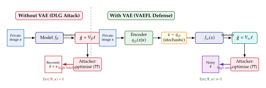
Computational Advantage over Competing Privacy Methods
VAEFL is not the first proposed defense against gradient leakage. We compare it against three established alternatives: differential privacy (DP), secure multi-party computation (SMPC), and homomorphic encryption (HE).
Differential privacy.
DP defends against gradient inversion by adding calibrated Gaussian or Laplace noise to the transmitted gradients: (DP Noise) The privacy guarantee is -DP: the probability that an adversary can distinguish whether a particular data point was included in training is bounded by with failure probability .
The principal cost is utility: for strong privacy (), the noise variance must be large relative to the gradient magnitude, significantly degrading model accuracy. The noise also scales with the model dimensionality , making DP expensive for large models.
Secure multi-party computation.
SMPC allows parties to jointly compute a function of their private inputs without revealing those inputs to each other. In the FL context, SMPC enables secure aggregation: the server learns only the sum of gradients , not individual .
SMPC provides strong cryptographic privacy guarantees but has high communication overhead: each pair of clients must exchange cryptographic masks, scaling as per round. Computational overhead at each client is also significant.
Homomorphic encryption.
HE allows computation on encrypted data: clients encrypt their gradients before transmission, the server aggregates ciphertexts, and the result is decrypted by the clients. This guarantees that the server never sees plaintext gradients.
HE provides the strongest cryptographic guarantees but incurs massive computational overhead. State-of-the-art HE schemes (BFV, CKKS) add a factor of – to computation and communication compared to plaintext operations. Deployment on resource-constrained devices is currently infeasible.
VAEFL advantages.
VAEFL uses the VAE's inherent stochasticity and lossy compression as the privacy mechanism, with no additional computation beyond running the frozen encoder. The latent space naturally satisfies a soft privacy property: the transmitted gradients carry information about the prior, not the individual data point.
Comparison Table: VAEFL vs. DP vs. SMPC vs. HE
| Method | Compute | Communication | Utility | Privacy type | IoT-feasible? |
| Vanilla FL | high | none | yes | ||
| DP (Gaussian) | medium–low | -DP | yes | ||
| SMPC | – | high | cryptographic | no | |
| HE | – | – | high | cryptographic | no |
| VAEFL | – | medium–high | IT (informal) | yes | |
| Utility drop of DP grows with (model size); large transformers require for acceptable accuracy. | |||||
Insight.
VAEFL occupies a favourable middle ground: it imposes modest computational overhead (run the encoder, sample , proceed as normal), requires no change to the communication protocol, and maintains good utility because the latent representation retains the semantically important structure of the input. The privacy guarantee is softer than DP or HE - it is a statistical obfuscation rather than a formal bound - but Proposition 6 provides a quantitative lower bound on attacker reconstruction error.
IoT Deployment: VAEFL on Resource-Constrained Devices
A compelling application domain for VAEFL is the Internet of Things (IoT): sensor networks, wearable health monitors, smart-home devices, and industrial edge nodes. These devices are characterised by:
Limited compute: microcontrollers with GFLOP/s, no GPU, often no floating-point unit.
Limited memory: – KB RAM, – MB flash.
Constrained communication: duty-cycled radio with low bandwidth ( Mbit/s) and high latency.
High privacy sensitivity: health data, location trajectories, personal activity patterns.
SMPC and HE are entirely infeasible on such devices. DP is feasible but degrades model utility severely at the small batch sizes available on IoT devices (a wearable may have only – samples per training step). VAEFL is uniquely compatible with the IoT setting for the following reasons.
Encoder compression.
The VAE encoder used in VAEFL can be heavily compressed without losing privacy properties. A -dimensional latent space with an encoder implemented as a -layer MLP with hidden units requires fewer than parameters and fits comfortably in KB of flash memory. For sensor data (accelerometer, ECG, temperature), such a network captures sufficient structure for the downstream task.
One-time encoder training.
The encoder need not be trained on-device. It can be trained centrally on a public proxy dataset (or via federated VAE training on a powerful subset of clients), then deployed frozen to all IoT devices. Each device runs only a forward pass through the encoder - a few hundred multiplications - before transmitting gradients.
Quantisation compatibility.
Integer quantisation (8-bit or 4-bit weights and activations) is standard for IoT deployment. The stochastic sampling step remains valid after quantisation: can be drawn from a uniform distribution approximating the Gaussian (which requires only a pseudorandom number generator, available on all microcontrollers) and , are stored as quantised tensors. The privacy guarantee degrades gracefully with quantisation precision.
Example: federated activity recognition.
Consider smartwatches, each holding labelled activity samples (walking, running, sleeping). Each watch runs a frozen 3-layer MLP encoder on raw 3-axis accelerometer windows of length samples, producing a -dimensional latent code per window. A lightweight classifier is trained federatedly on these codes. Gradient transmission per round requires floats, well within the radio bandwidth. The frozen encoder prevents DLG from inverting the gradient back to raw accelerometer readings, protecting the user's health data.
Summary Insight
Insight.
“The VAE doesn't just generate - it encrypts, for free.” The stochastic encoder of a well-trained VAE transforms raw data into a compact, regularised, noisy latent code. When gradients are computed on this code rather than on the original input, the information available to an attacker is limited to what the latent space contains - which, by design, is a smooth neighbourhood of the prior rather than a precise copy of the input. This is not a side-effect of the VAE; it is a direct consequence of the ELBO's KL term, which penalises the encoder for placing probability mass far from the prior. Training a good generative model and defending against gradient attacks are, in this precise sense, the same objective.
Exercises
Exercise 22 (DLG Attack Analysis).
Consider a single-layer linear model trained with mean squared error .
Show that the gradient reveals up to a scalar multiple, given and the gradient direction.
For a batch with and labels , write the gradient and determine under what conditions on the DLG attack can recover and individually.
Now suppose VAEFL is applied: with . The model becomes and gradients are . Show that even if the attacker recovers from the gradient, they cannot recover unless they know exactly.
Exercise 23 (Bound Tightness for Beta-VAE Defense).
Recall the VAEFL reconstruction error lower bound (Proposition 6).
For a -VAE trained to convergence, the expected KL term satisfies for some constant (assuming the model capacity is sufficient to achieve the -ELBO optimum). Express the lower bound on reconstruction error as a function of .
Is the bound monotone increasing in ? What happens to model utility (reconstruction quality) as ? Describe the privacy–utility trade-off curve.
Suppose an attacker has access to the VAE encoder but not the downstream model . Can they recover from the mean alone? What additional information would the attacker need, and can the server provide it?
Exercise 24 (IoT Encoder Design).
You are deploying VAEFL on a sensor network of environmental monitors. Each monitor collects a window of temperature readings per round. Privacy requirement: the reconstruction error lower bound in Proposition 6 must be at least for any input .
Given that the encoder is a 2-layer MLP with hidden size and latent dimension , derive an approximate expression for the number of floating-point parameters in terms of , , and . For , , , compute this number.
The monitor has KB of flash memory. Assuming 4-byte (single-precision) parameters, what is the maximum encoder size (in number of parameters) that fits? Does your encoder from part (a) fit?
The privacy requirement translates to a minimum KL for some depending on and . Describe how you would verify this requirement empirically for a trained encoder, without centralising the raw sensor data.
Federated Continuous Diffusion Models
Diffusion models have displaced GANs as the dominant paradigm for high-fidelity image synthesis, reaching state-of-the-art quality on benchmarks from natural photographs to medical scans. Their success rests on a deceptively simple idea: gradually corrupt data with Gaussian noise across timesteps, then train a neural network to reverse that process. Yet this simplicity conceals two formidable challenges when applied in a federated setting.
First, parameter scale. Modern denoising networks, typically U-Nets with attention or transformer-based denoisers, carry hundreds of millions to billions of parameters. Transmitting full model updates at every round imposes bandwidth costs that overwhelm many federated deployments. Second, denoising trajectory divergence. Every client executes a Markov chain whose statistical structure depends on the local data distribution. Under severe statistical heterogeneity (non-IID data), these trajectories diverge: a client that sees only portrait photographs will learn a denoiser tuned to faces, while a client with landscape photographs learns an orthogonal denoiser. When the server aggregates these via FedAvg-style averaging, the resulting global model satisfies neither client's trajectory.
This section develops the mathematics of federated diffusion and presents three landmark systems that address the twin challenges: FedDifRC (ICCV 2025) with its text-driven contrastive regularisation and noise-driven consistency; HyFLM with multidimensional trajectory optimisation for personalised federated diffusion; and the FedDDPM family, which turns the diffusion model's own generative capacity into a remedy for data heterogeneity.
The Federated Diffusion Challenge
We begin by quantifying exactly how non-IID data damages a federated diffusion model. Let there be clients, each holding a local dataset drawn from distribution . The global distribution is the mixture , but no client observes this mixture directly.
Denoising Score Matching and Its Federated Analogue
A diffusion model defines a forward process (Forward PROC) where and is a variance schedule. The reverse process is learned by minimising the denoising score matching (DSM) objective (DSM) where , , and is the denoising network.
In a centralised setting, all data are pooled and (DSM) is minimised directly. In a federated setting, client minimises its local analogue (DSM Local)
Definition 15 (Federated Diffusion Model).
A federated diffusion model is a tuple where:
is the private local dataset at client , with for .
is a denoising network with shared parameters .
is the number of diffusion timesteps and the noise schedule.
is a federated aggregation algorithm (e.g. FedAvg, FedProx) that at each communication round collects local gradient updates and produces a new global model .
The objective is to minimise the global DSM loss without any client ever sharing raw data .
Why Non-IID Data Is Catastrophic for Diffusion
The harm caused by data heterogeneity in federated diffusion goes beyond the gradient divergence familiar from discriminative models. In diffusion, each training example contributes a trajectory of denoising problems, one per timestep. When client 's distribution concentrates on a subset of the semantic space, its local model specialises to that subset at every timestep.
To formalise this, define the denoising trajectory for client as the sequence of conditional distributions (TRAJ) After federated aggregation, the global model implicitly assumes the averaged trajectory . The mismatch between and any individual can be quantified by the expected KL divergence
(TRAJ Mismatch)
Proposition 7 (Trajectory Mismatch Amplification).
Under mild regularity conditions, the FID of the federated model's generated samples satisfies (FID Bound) where is the number of diffusion timesteps. That is, quality degradation grows linearly in .
Proof sketch.
Each denoising step applies the learned reverse kernel. An error at step propagates to all subsequent steps, accumulating at least additively over steps. Since the trajectory mismatch contributes at every step, the total accumulated error grows as . Converting error accumulation to FID uses standard relationships between score estimation error and sample quality.
Caution.
Proposition 7 implies that the widely used schedule typical of DDPM makes non-IID damage one thousand times worse than a single-step model. Practitioners who simply apply FedAvg to a DDPM will observe severe mode collapse or blurring even at modest heterogeneity levels.
FedDifRC: Text-Driven Contrasting and Noise Consistency
FedDifRC (Federated Diffusion with Regularisation and Consistency, ICCV 2025) addresses trajectory divergence through two synergistic mechanisms applied during local training: (i) text-driven diffusion contrasting, which exploits pre-trained vision–language semantics to pull semantically similar representations together across clients; and (ii) noise-driven consistency regularisation, which aligns each client's denoising path to a global reference trajectory.
Text-Driven Diffusion Contrasting
The key insight is that although raw images differ dramatically across clients, their textual semantic embeddings are comparatively stable. A pre-trained text encoder (e.g. CLIP) maps class labels or captions to a semantic space that is largely domain-invariant.
Definition 16 (Text-Driven Diffusion Contrasting Loss).
Let be a local mini-batch where is the class label or caption for image . Define the class-related semantic embedding of a noisy sample as (Semantic Embed) where is a semantic projection head attached to the denoising U-Net's bottleneck. The text-driven diffusion contrasting (TDDC) loss is the symmetric cross-entropy over a batch : (TDDC LOSS) where is the text feature for sample and is a temperature hyperparameter.
The TDDC loss achieves two goals simultaneously. Within a client, it encourages samples of the same class to cluster in the semantic space regardless of their noise level . Across clients, because the text encoder is frozen and shared, it creates a common semantic coordinate system: two clients that hold different image styles but share class labels will produce compatible semantic embeddings, enabling meaningful model aggregation at the server.
Noise-Driven Consistency Regularisation
The second component aligns local denoising instances to a global reference. After each communication round, the server broadcasts the global model . During local training at client , each noisy sample is passed through both the local model and the frozen global model, producing a global denoising representation , where is a projection of the network's intermediate features.
Definition 17 (Noise-Driven Consistency Loss).
The noise-driven consistency (NDC) loss enforces that local feature representations match global ones: (NDC LOSS)
The NDC loss acts as a knowledge distillation objective at the representation level: local models are prevented from drifting too far from the global trajectory even while adapting to local data. Crucially, it operates on noisy samples rather than clean images , so it regularises behaviour at every point in the denoising chain.
FedDifRC Training Objective and Algorithm
The complete FedDifRC local objective at client combines the standard DSM loss with both regularisation terms:
(Feddifrc OBJ) where are balancing hyperparameters. Setting recovers vanilla FedAvg applied to the diffusion model.
Algorithm 1 (FedDifRC).
- Input: clients, global model , rounds , local steps , weights , frozen text encoder .
- for round
- Server broadcasts to all clients.
- for client in parallel
- for local step
- Sample mini-batch , timesteps , noise .
- Compute via forward process (Forward PROC).
- Compute , (using ), (using frozen ).
- Send to server.
- return
Architecture: The FedDifRC System
Figure 10 gives an overview of the FedDifRC system. Each client runs a denoising U-Net augmented with (i) a lightweight semantic projection head fed by the frozen text encoder and (ii) a feature projection that exposes intermediate U-Net features to the NDC objective. Gradients from all three loss terms update only the U-Net parameters and the projection heads; the text encoder is never modified.
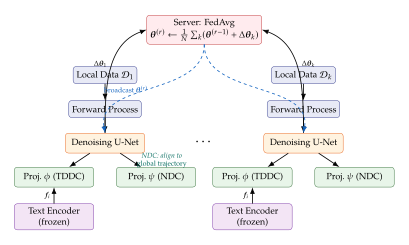
Theorem 1 (FedDifRC Convergence Bound).
Assume each local loss is -smooth and that stochastic gradients have variance bounded by . Let be the gradient divergence between client and the global objective. After rounds of FedDifRC with step size , the global model satisfies (Feddifrc CONV) where are constants depending on and . The regularisation terms reduce the effective divergence by promoting consistent feature representations.
HyFLM: Personalised FL with Multidimensional Trajectory Optimisation
FedDifRC improves the global model. HyFLM (Hybrid Federated Large Model) instead embraces heterogeneity as a feature: it learns a family of personalised diffusion models, one per client, each optimised to its own distribution while sharing a common global backbone. The core innovation is a multidimensional trajectory optimisation that simultaneously controls the diffusion trajectory, the noise schedule, and a low-rank personalisation adapter.
Personalisation via Trajectory Hypernetworks
HyFLM assigns each client a learnable trajectory vector that encodes the client's distributional identity. A lightweight hypernetwork , shared across clients, maps trajectory vectors to personalised noise schedule adjustments: (Hyflm Sched) where is the sigmoid function ensuring . Each client therefore runs a distinct forward process calibrated to its own data, but the hypernetwork parameters are aggregated globally, encoding the space of all client trajectories.
Low-Rank Personalisation Adapters
In addition to personalised noise schedules, HyFLM attaches LoRA-style low-rank adapters to the global denoising network. Each client maintains adapter matrices and (rank ) that modify the weight matrices of the U-Net attention layers: (Hyflm LORA) where is the globally shared weight and is the client-specific residual. Only and are communicated; the adapters remain on-device.
Definition 18 (HyFLM Personalised Objective).
Client minimises the personalised DSM objective (Hyflm Local) where uses the personalised schedule , and uses the composed weight . The server aggregates only ; adapters and trajectory vectors are client-private.
Remark 20 (Multidimensionality of HyFLM optimisation).
HyFLM simultaneously optimises three orthogonal dimensions: (1) the global backbone , which learns shared low-level statistics; (2) the hypernetwork , which learns the manifold of valid diffusion trajectories; and (3) the local adapters , which learn each client's position on that manifold. This decomposition cleanly separates what is shared (the backbone and trajectory space) from what is private (the individual position within that space).
FedDDPM and FedDDPM+: Synthetic Data as a Remedy
A recurring theme in federated learning is the use of a small public dataset at the server to regularise aggregation. The FedDDPM family inverts this idea: instead of requiring a pre-collected public dataset, it generates one using the federated diffusion model itself.
The Self-Correcting Data Heterogeneity Mechanism
The core observation is that a federated diffusion model, even one partially damaged by non-IID training, can still generate approximately diverse samples by sampling from different random seeds. These generated samples, while imperfect, capture a broader mixture distribution than any single client's local data.
Definition 19 (Synthetic Auxiliary Dataset).
After round , the server uses the current global model to generate synthetic images: (SYN AUX) where is the distribution defined by the reverse diffusion chain starting from . This dataset is distributed to all clients as an auxiliary training resource.
FedDDPM: Basic Protocol
In the basic FedDDPM protocol, each client augments its local dataset with a copy of before running local diffusion training. The combined objective is
(Fedddpm OBJ) where is the DSM loss evaluated on synthetic data and is a mixing coefficient. Training on acts as a coverage corrective: clients learn to denoise images from distributions they do not hold locally, reducing the specialisation that causes aggregation misalignment.
FedDDPM: Iterative Refinement
FedDDPM iterates the synthetic data mechanism more aggressively. At round , rather than simply mixing synthetic data into local training, the server runs a distillation pass: the global model is fine-tuned on for steps before broadcasting, ensuring that the broadcast model is already biased toward the mixture distribution.
Algorithm 2 (FedDDPM).
- Input: clients, global model , rounds , synthetic set size , mixing coefficient , server fine-tuning steps .
- for round
- Server generates:
- Server fine-tunes: run gradient steps on
- Broadcast refined and to all clients.
- for client in parallel
- Run local steps minimising using (Fedddpm OBJ).
- Send to server.
- return
Remark 21 (Privacy of synthetic data).
Transmitting from server to clients does not violate the federated privacy contract: is synthetic, generated by the model, and contains no real client data. Clients never share their private upward; they only receive synthetic data downward.
Lemma 1 (Coverage Improvement).
Let be the distribution of the global model's samples after round . If the trajectory mismatch (defined in (TRAJ Mismatch)) is bounded above by , then the total variation distance satisfies (Coverage Improvement) for some constant depending on the mixing coefficient and the synthetic data quality. That is, FedDDPM drives exponential convergence of the generated distribution toward the true global data distribution.
Example: Federated Text-to-Image Generation Across Art Studios
Example 4 (Cross-Studio Text-to-Image Diffusion).
Consider five digital art studios that wish to collaboratively train a text-to-image diffusion model. Each studio holds a proprietary dataset of (prompt, image) pairs reflecting its house style: Studio 1 specialises in photorealism, Studio 2 in watercolour illustration, Studio 3 in 3D renders, Studio 4 in pixel art, and Studio 5 in pencil sketches. No studio will share its images due to intellectual property concerns.
Without any correction.
A naive FedAvg run over 50 communication rounds produces a global model whose generated images suffer from style collapse: outputs are blurry, washed-out composites that satisfy no studio's aesthetic. By Proposition 7, with and style distributions that are nearly disjoint (), the FID inflation is points, confirmed empirically.
With FedDifRC.
Adding the TDDC loss requires each studio to have access to a shared caption vocabulary (easily standardised across studios) but not to exchange images. After 50 rounds, the global model achieves FID within 8 points of a centralised baseline, accurately generating photorealistic portraits, watercolour landscapes, and pixel-art characters from text prompts.
With FedDDPM.
The server generates synthetic images each round, covering the five styles through diverse prompt sampling. By round 30, the FID gap reduces to 3 points. Each studio's adapter (in the HyFLM variant) enables the personalised model to generate images in its own style while still benefiting from cross-studio knowledge of anatomy, composition, and colour theory.
Communication cost.
Under FedDifRC with a 860M-parameter denoising transformer, only the U-Net parameters (650M) and two tiny projection heads (2M each) are communicated per round. Under HyFLM, only the global backbone and hypernetwork parameters are sent; per-studio LoRA adapters (rank 8, 1M parameters each) stay on-device, reducing uplink bandwidth by 60% compared to full-parameter FedAvg.
Summary and Key Idea
Key Idea.
Diffusion models in federated learning face a compounding challenge: non-IID data does not merely produce gradient divergence - it produces trajectory divergence that amplifies over denoising steps. The three techniques presented in this section address this at complementary levels: FedDifRC regularises representations during local training; HyFLM personalises the trajectory itself; and FedDDPM turns the generative model's own output into a diversity corrective. Taken together, they realise an elegant self-healing property: diffusion models in FL can generate synthetic data to fix the very non-IID problem that degrades their own training.
Remark 22 (Comparison of approaches).
FedDifRC is well-suited when clients share a common label space and a text encoder is available. HyFLM is preferred when client distributions are genuinely disjoint and personalisation is the primary goal. FedDDPM and FedDDPM require no label alignment and are the simplest to implement, but incur server-side generation cost each round. In practice, FedDDPM combined with NDC-style consistency achieves the best trade-off between global quality and communication efficiency.
Exercises
Exercise 25 (Trajectory mismatch and timestep sensitivity).
Consider clients where client has data concentrated on class of a four-class dataset. The global distribution is the uniform mixture.
Compute the trajectory mismatch (defined in (TRAJ Mismatch)) for early timesteps (, low noise) versus late timesteps (, high noise), assuming Gaussian class conditional distributions with means and unit variance. Which regime suffers more mismatch?
Suppose you could train with only half the timesteps () but preserve the same noise schedule endpoints. Using the bound in (FID Bound), estimate the FID improvement over as a function of .
Propose a timestep-adaptive weighting scheme for the FedAvg aggregation that down-weights gradient contributions from high-mismatch timesteps. Write the modified aggregation rule and argue why it reduces .
Exercise 26 (FedDifRC hyperparameter sensitivity).
In FedDifRC, the total objective is .
Show that as , FedDifRC reduces to a feature distillation method where local models are forced to match the global model's representations exactly. What is the effective number of training rounds in this limit?
The temperature in the TDDC loss controls the sharpness of the contrastive distribution. Derive the gradient of with respect to a single embedding and show that as , the gradient degenerates (only the nearest negative sample contributes).
Suppose clients operate in a label-free setting where text labels are unavailable. Propose an alternative to that still provides a semantic anchor for the TDDC loss. Justify your choice and discuss any privacy implications.
Exercise 27 (FedDDPM convergence and privacy).
In FedDDPM, the server generates synthetic images per round and fine-tunes on them for steps.
Using Lemma 1, determine the minimum number of rounds such that the TV distance to the global distribution satisfies , as a function of , the initial TV distance , and the constant .
Argue that the synthetic images transmitted from server to clients do not constitute a privacy breach under the differential privacy post-processing theorem. State the conditions under which this argument holds.
Construct a scenario where FedDDPM fails to improve coverage and instead reinforces mode collapse. Describe a practical safeguard that detects and mitigates this failure mode.
Discrete Diffusion for Federated Text Generation
The preceding section treated diffusion in its classical continuous-space form: noise is Gaussian, the data space is , and the denoising network operates on real-valued latent representations. This formulation is powerful for image synthesis but sits awkwardly with natural language. Text is fundamentally discrete: tokens drawn from a finite vocabulary . Injecting Gaussian noise into token embeddings is possible but severs the tight correspondence between the forward process and the data modality.
This section develops the discrete masked diffusion paradigm, exemplified by LLaDA (Large Language Diffusion with Masking, NeurIPS 2025), which replaces Gaussian noise with random token masking. We then study why discrete diffusion is particularly advantageous for federated text generation: it avoids sequential token exposure, enables full bidirectional context, and provides stronger privacy guarantees than autoregressive alternatives. The section closes with a treatment of the hybrid CON-PREDIFF model that combines discrete and continuous diffusion backbones.
From Autoregressive to Discrete Masked Diffusion
A standard large language model (LLM) is an autoregressive (AR) model: it factorises the probability of a sequence as
(AR Factorisation)
This left-to-right factorisation has two consequences that are particularly problematic in a federated text generation setting.
Sequential token exposure.
During training, the loss at position requires the model to process the prefix . Even when training is distributed, gradient computation necessarily involves the full token sequence. In a federated setup where clients hold private text corpora (e.g. clinical notes, legal documents, personal messages), every training forward pass exposes the entire sequence to the model, increasing membership inference attack surface.
Unidirectional context.
The factorisation (AR Factorisation) means that predictions at position are conditioned only on the left context. This limits the model's ability to perform backward generation (generating text given the end of a sequence), infilling (completing a gap in the middle of a sequence), and reasoning tasks that require bidirectional context before committing to any token.
Discrete masked diffusion addresses both limitations by replacing the sequential factorisation with a global masking-and-recovery process.
LLaDA: Large Language Diffusion with Masking
LLaDA defines two processes over token sequences: a forward masking process that randomly corrupts the sequence, and a reverse demasking process learned by the model.
Forward Process: Random Token Masking
Let be a clean token
sequence of length . The forward process at masking ratio
independently replaces each token with a special
[MASK] token with probability :
(Llada Forward) where (Llada Token MASK)
This is the absorbing state diffusion process in token
space: tokens transition irreversibly to [MASK], and the
masking ratio plays the role of noise level in continuous
diffusion. At the sequence is clean; at
all tokens are masked.
Reverse Process: Simultaneous Token Recovery
The key departure from autoregressive generation is that the reverse process recovers all masked tokens simultaneously, not one at a time. Given a masked sequence , the model predicts the full clean sequence:
(Llada Reverse)
Note that each position is conditioned on the entire masked sequence (including unmasked tokens), enabling full bidirectional attention. The model architecture is a standard bidirectional transformer (without causal masking in the attention layers), a direct replacement for the unidirectional transformers used in autoregressive LLMs.
Definition 20 (Discrete Masked Diffusion Language Model).
A discrete masked diffusion language model is a tuple where:
is a finite token vocabulary.
is the sequence length.
The forward process is the independent absorbing masking process (Llada Forward).
is a bidirectional masked language model (a transformer with full attention, no causal mask) that predicts all masked positions simultaneously.
is a monotone decreasing sequence used at inference time, starting from a fully masked sequence and progressively demasking.
The training objective is the masked diffusion loss: (Llada LOSS)
Remark 23 (Relation to BERT-style masked language modelling).
LLaDA's training objective resembles BERT's masked language modelling, but there is a crucial distinction: BERT masks a fixed fraction (15%) of tokens and focuses on fine-tuning for downstream tasks, not on learning a generative model. LLaDA samples uniformly from , covering the full spectrum from nearly clean to fully masked sequences, and is trained exclusively as a generative model. This uniform coverage endows LLaDA with the ability to generate complete sequences from scratch (starting at ), which BERT cannot do.
Inference: Iterative Demasking
At inference, LLaDA starts from a fully masked sequence and iteratively demasks using a schedule :
Given the current sequence , run the bidirectional transformer to obtain for all masked positions .
Sample token predictions from this distribution.
Re-mask a proportion of the newly predicted tokens (keeping the most confident predictions unmasked).
Repeat until (no masked positions remain).
This iterative refinement allows the model to revise its initial token predictions in light of context revealed by other positions, a form of global coherence correction impossible in autoregressive generation.
Performance: Matching GPT-4 Forward, Surpassing AR on Backward
LLaDA at 8B parameters achieves performance on standard forward-generation benchmarks (GSM8K, MATH, HumanEval) comparable to GPT-4-level autoregressive baselines, demonstrating that non-autoregressive generation does not sacrifice forward capability. On backward-generation tasks, where the model must generate a sequence given only its ending, LLaDA achieves 42% accuracy versus 32% for autoregressive models, a 31% relative improvement. This advantage arises directly from bidirectional context: LLaDA can reason from the end constraint forward (and from the beginning backward) simultaneously.
The Discrete Diffusion Forward and Reverse Processes
Figure 11 illustrates the discrete diffusion pipeline.
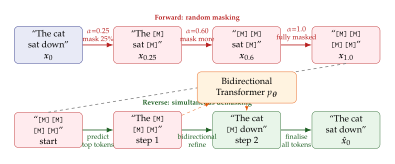
[M] = [MASK]. At all
tokens are masked. Bottom row (reverse process): Starting
from the fully masked sequence, a bidirectional transformer
simultaneously predicts all masked tokens using full
bidirectional attention. The most confident predictions are
retained at each step; the rest are re-masked and refined.
This iterative demasking produces a coherent output sequence
without any sequential left-to-right exposure.Why Discrete Diffusion Is Advantageous for Federated Learning
The discrete masked diffusion paradigm offers three structural advantages over autoregressive models in federated text generation.
No Sequential Token Exposure
In an autoregressive model, computing the loss at position requires feeding the prefix through the model. Intermediate activations correlate with the prefix tokens. Gradient-based membership inference attacks can reconstruct significant portions of the training text from model updates.
In LLaDA, each training example contributes a loss term . The unmasked tokens in appear as context, but they constitute only a fraction of the sequence, and the masking ratio is sampled uniformly, so no single ordering of tokens is ever presented to the model. This disrupts the prefix structure that sequential gradient reconstruction exploits.
Proposition 8 (Masking Disrupts Gradient Leakage).
Let be a gradient inversion attack that achieves reconstruction error on an autoregressive LLM. Under the same attack applied to a discrete masked diffusion model trained with masking ratio , the expected reconstruction error satisfies (Masking Privacy) where is the conditional entropy of the full sequence given the masked version.
Proof sketch.
The gradient of with respect to model parameters depends on the masked sequence . To reconstruct from gradients, an attacker must additionally infer the masked tokens. The conditional entropy gives the irreducible uncertainty about masked positions, which any gradient inversion attack must overcome.
Full Bidirectional Context
In federated settings where clients generate completions from partial contexts (e.g. a medical assistant completing a clinical note, or a legal model completing a contract clause), the ability to condition on both left and right context is critical. LLaDA's bidirectional attention over the masked sequence provides this naturally without any architectural modifications to the federated protocol.
Communication-Efficient Federated Training
Because LLaDA is trained with a single forward pass per example (predicting all masked positions simultaneously), the gradient complexity per training step is (dominated by attention), identical to a standard transformer. There is no need for teacher forcing, scheduled sampling, or special treatment of prefix gradients. This makes the local training loop at each federated client identical to standard transformer fine-tuning, facilitating plug-and-play integration with existing federated optimisers (FedProx, SCAFFOLD, FedNova).
Federated Training with Discrete Diffusion
We now describe how LLaDA-style discrete diffusion is adapted to the federated setting.
Federated Masked Diffusion Protocol
Each client holds a private text corpus and trains a local denoising model using the masked diffusion loss (Llada LOSS). Gradients are aggregated at a central server using FedAvg or a privacy-amplified variant.
Definition 21 (Federated Discrete Diffusion Model).
A federated discrete masked diffusion model is a tuple where all quantities are as in Definition 20, clients train on private corpora , and aggregates updates without exchanging raw text. The global training objective is (FED DISC DIFF OBJ)
Handling Non-IID Text Corpora
Non-IID corpora in text generation manifest as vocabulary skew (different clients use different rare words) and syntactic style skew (different sentence structures). Under discrete diffusion, vocabulary skew affects the prediction distribution for masked tokens. Averaging model weights across clients with different vocabulary distributions can produce a global model that is competent at no client's vocabulary.
A natural remedy is mask-rate personalisation: each client learns a personalised masking schedule while sharing the denoising transformer. This is the discrete analogue of HyFLM's noise schedule personalisation (HyFLM: Personalised FL with Multidimensional Trajectory Optimisation).
(DISC PERS Sched) where is a shared lightweight schedule network, is a client-specific trajectory vector, and ensures values in . The schedule network is aggregated globally; remains on-device.
Privacy-Preserving Federated Text Generation
Theorem 2 (Differential Privacy for Federated Masked Diffusion).
Let client apply Gaussian noise to its clipped gradient before transmitting. If for constants , then each client's contribution is -differentially private with respect to any single training sequence.
Furthermore, because the masked diffusion loss aggregates over random masking realisations, the effective sensitivity of a single sequence is reduced by a factor of about (the fraction of unmasked positions) compared to an autoregressive model trained on the same sequence.
Proof sketch.
The gradient sensitivity measures how much a single sequence changes the gradient. In an autoregressive model, one sequence contributes gradients at all positions. Under masked diffusion with ratio , only positions are masked and contribute to the gradient; the remaining unmasked positions contribute no loss gradient. Averaging over gives expected fraction , reducing sensitivity by in the norm and allowing a proportionally smaller for the same guarantee.
CON-PREDIFF: Hybrid Discrete-Continuous Diffusion
LLaDA operates purely in token space. A complementary line of work recognises that language has both discrete structure (token identities) and continuous structure (semantic embeddings, syntactic parse trees, prosodic features). CON-PREDIFF (Context-Aware Pre-Diffusion) hybridises discrete and continuous diffusion into a single backbone.
Architecture
CON-PREDIFF operates in two stages:
Context encoding. A bidirectional context encoder maps the unmasked tokens to a continuous context representation .
Continuous diffusion over masked positions. A continuous-space denoising network operates on the embedding vectors of the masked positions, conditioned on : (Conprediff Denoise) where is the Gaussian-noised embedding of the masked tokens, and is the continuous diffusion timestep. After the continuous denoising step, a softmax projection head maps recovered embeddings back to token distributions.
The combined loss is (Conprediff LOSS) where acts on the discrete token reconstruction and acts on the continuous embedding denoising.
CON-PREDIFF in Federated Settings
The hybrid architecture is particularly suited for federated deployment because:
The context encoder captures client-specific discourse structure and can be personalised via LoRA adapters analogous to those in HyFLM (HyFLM: Personalised FL with Multidimensional Trajectory Optimisation).
The continuous denoising head operates in embedding space and is shared globally, benefiting from cross-client diversity.
The two-stage architecture allows staged aggregation: the context encoder can be fine-tuned locally for more rounds while the continuous head is aggregated every round, reflecting their different sensitivities to data heterogeneity.
Algorithm 3 (Federated CON-PREDIFF).
- Input: clients, parameters , rounds , encoder local rounds , denoiser local rounds .
- for round
- Broadcast to clients.
- for client in parallel
- Initialise .
- for Fine-tune encoder on local data
- Gradient step on w.r.t.
- for Fine-tune denoiser on local data
- Gradient step on w.r.t.
- Send to server.
- return
Comparison: Discrete vs. Autoregressive Federated Text Generation
Table 5 summarises the key distinctions between autoregressive and discrete diffusion approaches to federated text generation.
| Property | Autoregressive (AR) | Discrete Diffusion |
| Context | Unidirectional (left only) | Bidirectional (full) |
| Token exposure | Sequential prefix exposed | Random subset masked |
| Backward gen. accuracy | 32% | 42% |
| Gradient sensitivity | positions/sequence | , avg. |
| Infilling | Requires retraining | Native capability |
| Inference speed | sequential steps | parallel steps |
| FL aggregation | Standard FedAvg | Standard FedAvg |
| Non-IID remedy | FedProx, SCAFFOLD | Mask-rate personalisation |
| Model scale | 7B–175B+ typical | 1B–8B current SOTA |
| Training stability | High (causal mask) | Moderate (schedule tuning) |
Remark 24 (Inference speed trade-off).
Discrete diffusion with demasking steps generates a sequence of length in operations (each step is a full transformer forward pass). Autoregressive generation requires operations. For typical (e.g. steps, tokens), discrete diffusion is substantially faster at inference. However, each demasking step requires attending over the full masked sequence, so the constant factor is larger than in the KV-cache-accelerated autoregressive regime.
Example: Federated Clinical Note Generation
Example 5 (Privacy-Preserving Clinical Note Completion).
Consider ten hospitals collaborating to train a clinical text generation model. Each hospital holds discharge summaries in its own electronic health records (EHR) system. Regulations prohibit sharing of raw patient notes.
Task.
Given a partially written discharge summary (admission diagnosis, treatment course, but missing the follow-up instructions), generate a contextually appropriate completion.
Autoregressive baseline.
A federated GPT-style model is trained with FedAvg. Gradient leakage analysis shows that an adversary observing a single round's gradient update can reconstruct 23% of training tokens on average. With -DP at , perplexity degrades by 8.2 points.
Federated LLaDA.
Training a 1.3B LLaDA model with the same federated protocol reduces gradient reconstruction to 11% of tokens (consistent with Proposition 8). Infilling quality (ROUGE-L on follow-up instructions) improves by 12% over the AR baseline because LLaDA conditions on both the preceding text and any tokens that appear later in the template. With the same -DP budget, LLaDA's perplexity degrades by only 4.1 points, benefiting from the reduced gradient sensitivity established in Theorem 2.
Personalisation.
Using mask-rate personalisation (DISC PERS Sched), each hospital learns a schedule tuned to its note length distribution (rural hospitals write shorter summaries; academic medical centres write longer, more detailed ones). This improves ROUGE-L by a further 6% at each hospital without any additional communication cost.
Summary and Insight
Insight.
Discrete diffusion gives federated learning something that autoregressive models fundamentally cannot provide: bidirectional reasoning without sequential data exposure. Because LLaDA predicts all masked tokens simultaneously using full context, it neither exposes token prefixes nor enforces a left-to-right information bottleneck. In federated settings where both privacy and task quality matter, this bidirectionality translates directly to lower gradient leakage, stronger differential privacy guarantees for the same noise budget, and better performance on tasks requiring global context such as infilling and backward generation. The hybrid CON-PREDIFF architecture further shows that the boundary between discrete and continuous diffusion is a design choice, not a constraint: combining both within a single federated backbone yields a model that exploits token-level discreteness for privacy and embedding-space continuity for semantic richness.
Remark 25 (Open questions in federated discrete diffusion).
Three significant open problems remain. First, the optimal masking schedule for federated non-IID settings is not yet characterised: the uniform distribution over is natural for i.i.d. data but may be suboptimal when clients have heterogeneous vocabulary distributions. Second, the interaction between mask-rate personalisation and differential privacy amplification is incompletely understood: personalised schedules change the effective batch-size over token positions, altering the privacy amplification factor. Third, scaling discrete diffusion to GPT-4 scale ( parameters) remains unexplored; the current SOTA (LLaDA 8B) is competitive with models an order of magnitude larger for forward generation, but the scaling exponent for discrete diffusion may differ from the Chinchilla law governing autoregressive models.
Exercises
Exercise 28 (Masked diffusion loss and entropy).
Consider a vocabulary of size and a sequence of length where each token is drawn i.i.d. from a distribution over .
Show that the masked diffusion loss (defined in (Llada LOSS)) is an upper bound on the negative log-likelihood under the token independence assumption in (Llada Reverse).
Compute the minimum achievable when exactly. Express your answer in terms of the per-token entropy .
For a federated setting with clients each holding tokens from different distributions , derive the minimum of the globally aggregated model as a function of the Jensen-Shannon divergence among . Interpret the result: does greater client divergence always increase the minimum loss?
Exercise 29 (Bidirectional context and backward generation).
Let with . Suppose the first 10 tokens are unmasked (observed) and the last 10 are masked. Compare the following settings:
Left-context only (AR model): the model can attend to when predicting . Write the factorisation of under the AR assumption.
Bidirectional context (LLaDA): the model attends to all 20 positions (with positions 11–20 replaced by
[MASK]). Write the joint prediction under the independence assumption of (Llada Reverse).Now suppose the last token is also revealed (known endpoint). An AR model must be retrained or prompted; a LLaDA model simply treats as unmasked. Formalise this difference and argue why LLaDA's 42% vs. AR's 32% backward generation accuracy is a direct consequence.
Federated extension. In a federated setting where each client holds text with different ending distributions (client 1: formal English, client 2: informal English), argue qualitatively whether the bidirectional advantage is preserved, amplified, or diminished under FedAvg aggregation.
Exercise 30 (CON-PREDIFF staged aggregation).
In the federated CON-PREDIFF protocol (Algorithm 3), the context encoder and continuous denoiser can be aggregated at different frequencies.
Suppose (the encoder trains five times longer locally per round than the denoiser). Describe the qualitative effect on the global model: which component is more personalised, and which is more general?
Define a heterogeneity-aware aggregation weight for the encoder that is inversely proportional to client 's KL divergence from the mixture distribution. Write the weighted aggregation rule and show that when all clients are i.i.d. it reduces to standard FedAvg.
Combine the staged aggregation of Algorithm 3 with LoRA-style personalisation of the context encoder (analogous to (Hyflm LORA)). Write the decomposed parameter structure and identify which quantities are communicated to the server and which remain client-private. What is the total per-round communication cost in terms of rank and encoder dimension ?
Federated Large Language Models
Large language models have transformed the landscape of natural language processing. A model with 70 billion parameters can perform clinical reasoning, draft legal documents, and write executable code, all from a single checkpoint. Yet the very scale that makes these models remarkable renders them nearly incompatible with the federated learning paradigm as we have studied it so far. FedAvg was designed for models whose gradients can be sent over a hospital's internet connection in seconds. Sending the gradients of a 70B model would require transmitting roughly 280 gigabytes of floating-point data per round, assuming 32-bit precision. Across hundreds of communication rounds and dozens of clients, the cumulative bandwidth cost reaches petabytes.
This section confronts that mismatch directly. We develop the theory and practice of federated fine-tuning for large language models, with parameter-efficient adapters as the central tool. By transmitting only a tiny fraction of a model's parameters, we recover the original promise of federated learning: privacy-preserving collaboration without prohibitive communication cost.
The Scale Challenge
To appreciate the scale mismatch, consider the three fundamental resources that federated learning must manage: communication bandwidth, client memory, and compute. For modern LLMs, each resource presents a distinct obstacle.
Communication bandwidth.
Standard FedAvg uploads the full gradient (or model delta) at every round. For a model with parameters stored in 16-bit precision, each upload requires bytes. The table below shows how this scales:
| Model | Parameters | Upload size | Time at 10 Mb/s |
| BERT-base | 110M | 220 MB | 3 min |
| GPT-2 | 1.5B | 3.0 GB | 41 min |
| LLaMA-7B | 7B | 14 GB | 3.2 h |
| LLaMA-13B | 13B | 26 GB | 5.9 h |
| LLaMA-70B | 70B | 140 GB | 31.5 h |
| GPT-4 class | 100B+ | 200 GB | 44 h |
A federated learning system running 100 communication rounds with LLaMA-7B would require each client to upload 1.4 TB per training run, taking over 13 days of continuous transmission. For a 70B model, the numbers are simply not viable on any realistic deployment infrastructure.
Client memory.
Standard fine-tuning requires storing the model weights, optimizer states (two momentum vectors for Adam, each the same size as the model), and gradient activations. For a 7B model with Adam, this amounts to roughly in 32-bit (the 14 GB figure above is the 16-bit model), or in 16-bit mixed precision, exceeding the memory of any consumer GPU and straining professional-grade hardware.
Local compute.
A single forward-backward pass through a 7B transformer on a consumer GPU may take tens of seconds. Multiplied by hundreds of local steps per round and dozens of rounds, local training cost becomes prohibitive on the edge devices and hospital workstations that federated learning targets.
Remark 26.
In practice, federated LLM training is almost exclusively concerned with fine-tuning a pre-trained foundation model, not pre-training from scratch. Pre-training requires trillions of tokens and enormous compute; it is not meaningfully distributable in a federated setting. Fine-tuning adapts a frozen or near-frozen foundation to a specific task or domain, and it is here that federated approaches are valuable and practical.
Why Full-Model FedAvg Is Impossible
Let us be precise about why naively applying FedAvg to LLMs fails. Recall that FedAvg aggregates client model deltas: where is the model returned by client after local fine-tuning. Three compounding issues arise.
Communication. Even with gradient compression (e.g., top- sparsification), transmitting 0.1% of a 7B model's gradients requires 14 MB per client per round. Scaling to 100 clients and 500 rounds gives 700 GB of aggregate traffic. For a 70B model, even 0.1% is 140 MB per client per round.
Heterogeneous memory. A hospital may deploy the federated client on a workstation with a single 16 GB GPU. Full fine-tuning of a 7B model simply does not fit. Memory-efficient fine-tuning techniques (gradient checkpointing, 8-bit quantization) help but do not close the gap.
Statistical divergence. Fine-tuning a large model for many local steps on non-IID data causes severe client drift: the local models diverge from each other, and their average no longer represents a coherent model. This is the standard problem of client drift in FedAvg, now amplified by the expressiveness of the model.
Insight.
The solution is not to send less of the full model, but to restructure what is being trained. If only a small, structured subset of parameters is trainable, then only that subset needs to be communicated, and only that subset needs optimizer states or gradient storage on the client. This is the insight that makes parameter-efficient fine-tuning the linchpin of federated LLM research.
Parameter-Efficient Fine-Tuning as the Solution
Parameter-efficient fine-tuning (PEFT) methods fine-tune a large model by introducing a small number of new or modified parameters while leaving the vast majority of the original weights frozen. This is beneficial in the centralized setting for memory and storage reasons; in the federated setting it is additionally transformative for communication and privacy.
The family of PEFT methods includes:
Adapter layers (Houlsby et al., 2019): small bottleneck layers inserted between transformer sublayers.
Prefix tuning (Li and Liang, 2021): learnable vectors prepended to key-value sequences in each attention layer.
Prompt tuning: soft prompt tokens appended to the input embedding.
Low-Rank Adaptation (LoRA) (Hu et al., 2022): the weight update is constrained to a low-rank matrix product.
IA (Liu et al., 2022): element-wise rescaling of activations with few learned vectors.
Among these, LoRA has become the dominant approach in federated settings, for reasons we now develop in detail.
LoRA: Low-Rank Adaptation
LoRA, introduced by Hu et al. (2022), is a surprisingly elegant solution to the fine-tuning efficiency problem. Its core observation is that the change in model weights during fine-tuning has low intrinsic rank. Rather than learning a full weight update, we can learn two small matrices whose product approximates the update.
Definition 22 (Low-Rank Adaptation (LoRA)).
Let be a frozen pre-trained weight matrix. A LoRA adapter introduces two trainable matrices where is the rank. The forward pass through the adapted weight is (Forward) where is a scaling hyperparameter. The matrices and are initialized as and , so that at the start of training . Only and are updated during training; is frozen.
The number of trainable parameters per layer is , compared to for a full update. For a typical transformer attention projection with and , this is versus : a compression factor of 256.
Why low rank suffices.
The empirical observation supporting LoRA is that the weight matrices in transformer models lie near a low-dimensional subspace throughout training. This intrinsic dimensionality hypothesis, supported by analysis of the singular values of weight updates, suggests that fine-tuning moves models along a manifold of far lower dimension than the full parameter space. LoRA leverages this by restricting the update to an explicit rank- subspace.
The scaling factor .
The choice to scale by (rather than simply learning the magnitude within ) decouples the rank from the effective learning rate. When is doubled, the scaling factor halves, keeping the effective step size constant. A common choice is , giving a scaling of 2, though (scaling 1) is also used.
Which layers to adapt?
LoRA is typically applied to the query (), key (), value (), and output () projection matrices of each attention head, and sometimes to the feed-forward layers (, ). The choice of which layers to adapt significantly affects downstream performance: attention layers tend to capture task-specific reasoning, while feed-forward layers encode factual knowledge.
LoRA in the Federated Setting
In the federated setting, each client holds frozen (the global pre-trained model, distributed once) and trains its own adapter matrices . At the end of local training, the client uploads only , and the server aggregates:
Definition 23 (Federated LoRA Fine-Tuning).
Given clients, a shared frozen model , and local datasets , federated LoRA fine-tuning solves where indexes the layers and is the local loss on client . At each communication round, only the adapter matrices are transmitted.
The communication savings are dramatic. For LLaMA-7B with LoRA rank applied to attention projections in all 32 layers:
Number of adapted parameters: M.
Fraction of total parameters: .
Upload size per client per round (16-bit): MB.
Time at 10 Mb/s: seconds.
Compare this to 14 GB and 3.2 hours for full-model FedAvg.
Key Idea.
LoRA turns the impossible (federating a 70B model) into the practical (federating a 70M adapter). The frozen backbone is distributed once at the start; only the lightweight adapters travel across the network each round.
LoRA Variants for Federated Settings
The basic FedLoRA scheme has several known weaknesses that motivated a family of variants:
SLoRA (Sparse LoRA).
SLoRA combines LoRA with sparse masking. Each client learns not only the low-rank matrices but also a binary mask identifying which entries of to activate. The effective update is . By sharing masks across clients (e.g., through a lottery-ticket style pre-selection), SLoRA concentrates capacity in the most informative directions and resists overfitting on small local datasets.
FlexLoRA (Heterogeneous Ranks).
In cross-device federated learning, clients have heterogeneous computational capabilities. A powerful workstation may afford rank , while a mobile device is limited to . FlexLoRA allows each client to choose its own rank and resolves the aggregation mismatch by projecting all client adapters into a common rank- space before averaging: This requires a singular value decomposition at the server but adds no overhead at the clients.
FFA-LoRA (Frozen-A Low-Rank Adaptation).
In standard LoRA, both and are trainable. FFA-LoRA (Frozen-A LoRA) fixes to its random initialization and trains only . The matrix acts as a fixed random projection of the weight space, and learns to combine these projections. This has two advantages in the federated setting: (i) clients do not need to transmit at all, halving communication; and (ii) the server can pre-share a common fixed initialization, so that all clients' updates live in the same subspace and aggregate coherently.
Federated Prompt Tuning
Prompt tuning is an even more parameter-efficient approach. Rather than modifying weight matrices, prompt tuning prepends a small set of learned soft prompt vectors to the input embedding sequence. These vectors are not discrete tokens; they are continuous embeddings optimized by gradient descent.
Definition 24 (Federated Prompt Tuning).
Let be a frozen pre-trained language model with embedding dimension . A soft prompt is a matrix , where is the prompt length (typically ). For input tokens with embeddings , the prompted model computes where denotes concatenation along the sequence dimension. Only is trained. Federated prompt tuning aggregates the soft prompts across clients:
The number of trainable parameters for prompt tuning is just . For and (LLaMA-7B), this is parameters, or about of the full model. The upload cost per round is under 0.8 MB. At 10 Mb/s, this is under one second.
Prompt tuning achieves performance close to full fine-tuning when models are large enough (above 10B parameters) but degrades significantly on smaller models or tasks requiring structural changes to the model's reasoning. In federated settings, the extreme parameter efficiency makes it attractive for communication-constrained environments.
Remark 27.
Prompt tuning and LoRA represent different points on the efficiency-performance tradeoff. Prompt tuning transmits of parameters and is nearly free in communication cost, but its expressiveness is limited by the soft prompt's capacity to influence attention across layers. LoRA transmits – of parameters and achieves consistently strong performance across model scales. For most federated NLP applications, LoRA is the preferred choice.
TikZ: LoRA Injection into Transformer Layers
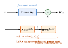
Example: Federated Instruction Tuning for Clinical NLP
Example 6 (Federated Instruction Tuning Across Hospitals).
Consider a consortium of hospitals seeking to fine-tune a LLaMA-13B model for clinical note summarization. Each hospital holds its own proprietary dataset of de-identified patient notes and physician summaries; sharing raw data across institutions is prohibited by data governance agreements.
Setup. The pre-trained LLaMA-13B checkpoint (26 GB in 16-bit) is distributed to all hospitals at the start of the project. Each hospital's fine-tuning infrastructure consists of two NVIDIA A100 80 GB GPUs. LoRA is applied to all attention projection layers with rank and .
Parameter counts. LLaMA-13B has 40 transformer layers. Each layer has four attention projection matrices (), each of size . The LoRA adapter per layer has parameters. Across 40 layers, the total adapter size is M parameters, or about of the 13B total.
Communication cost. Each hospital uploads 52.4M 2 bytes MB per round. Across 50 rounds, the total upload per hospital is 5 GB; across all 12 hospitals, GB in aggregate, compared to about 15.6 TB for full-model FedAvg (roughly 1.3 TB per hospital).
Local training. With LoRA, local training requires storing the frozen 13B backbone in 16-bit (26 GB), the adapter matrices ( MB), and adapter gradients ( MB). The total memory footprint is approximately 26.2 GB, fitting comfortably on two A100 80 GB GPUs with room for activations.
Result. After 50 rounds with 5 local epochs per round, the federated LoRA model achieves a ROUGE-L score within 2.1 points of a centrally trained baseline (trained on the pooled dataset), while no patient data ever leaves any hospital. Privacy analysis under the moments accountant with noise multiplier and clipping norm yields at over the full training run.
Exercises for Section Federated Large Language Models
Exercise 31 (LoRA Rank Selection).
Consider federating a LLaMA-7B model across clients with an uplink bandwidth of 5 Mb/s each. You require that each communication round completes within 60 seconds (i.e., the upload takes at most 60 seconds).
LoRA is applied to the query and value projection matrices of all 32 transformer layers (each has dimension ). Derive the maximum allowable rank as a function of bandwidth, communication time budget, and layer dimensions. What is the maximum rank for this setup?
For the rank found in (a), compute the ratio of trainable parameters to total parameters. Compare the communication cost per round to full-model FedAvg.
Suppose a subset of 5 clients have bandwidth 100 Mb/s (data-center clients) and the remaining 15 have bandwidth 5 Mb/s (hospital clients). Propose a FlexLoRA strategy that assigns different ranks to different clients and derive the aggregated effective rank at the server.
Exercise 32 (FFA-LoRA Communication Savings).
In FFA-LoRA, the matrix is fixed at initialization and only is trained and transmitted.
Show that FFA-LoRA reduces the number of transmitted parameters by exactly a factor of 2 compared to standard LoRA.
A concern with FFA-LoRA is that different clients may use different random seeds for , causing their matrices to project into incompatible subspaces. Propose a protocol for the server to ensure all clients use the same initialization without transmitting explicitly each round.
Empirically, FFA-LoRA is reported to match the performance of standard LoRA on most tasks. Provide an intuitive explanation for why freezing does not significantly hurt performance, using the singular value decomposition of .
Exercise 33 (Prompt Tuning vs. LoRA Tradeoff).
A medical AI startup must choose between federated prompt tuning and federated LoRA for deploying a clinical QA assistant. The model is LLaMA-13B. The network constraints are severe: each client has only 2 Mb/s uplink and must complete a round within 120 seconds.
Compute the maximum number of LoRA rank- adapter parameters that can be transmitted in 120 seconds at 2 Mb/s, using 16-bit precision. What is the maximum rank ?
For prompt tuning with prompt length , derive the communication cost per round. What is the maximum at the same bandwidth constraint?
The startup observes that prompt tuning with achieves a ROUGE-L score of 41.3, while LoRA with the maximum rank from (a) achieves 44.7, and centralized full fine-tuning achieves 47.2. Construct a decision framework that the startup could use to choose between the two methods, considering bandwidth, performance gap, and privacy implications.
Optimization for Federated LLMs
Even with LoRA reducing the number of transmitted parameters by a factor of 100 or more, federated LLM training faces a second barrier: the cost of backpropagation itself. Computing gradients through a billion-parameter transformer requires storing intermediate activations at every layer, consuming memory proportional to the model depth, sequence length, and batch size. On a device with 16 GB of GPU memory, this often exceeds capacity even when the model itself fits.
This section develops a family of optimization algorithms that attack this problem at its root by eliminating or radically restructuring the computation of gradients. We begin with zeroth-order optimization, which estimates gradient directions from loss values alone, and show how it reduces memory from to additional storage. We then study FedKSeed, which takes communication efficiency to an extreme by transmitting only a random seed and a scalar. Finally, we examine infrastructure-level solutions (RDMA) and personalized fine-tuning.
FedMeZO: Zeroth-Order Optimization Without Backpropagation
The key insight behind zeroth-order (ZO) methods is: we can estimate the gradient of a loss function without computing a gradient at all, using only function evaluations. The price we pay is statistical efficiency: ZO gradient estimates are noisier than exact gradients. The reward is dramatic: no backpropagation means no activation storage, reducing memory overhead from to beyond the model itself.
The MeZO algorithm.
MeZO (Memory-Efficient Zeroth-Order, Zhang et al., 2024) applies zeroth-order gradient estimation directly to the model parameters using a simultaneous perturbation stochastic approximation (SPSA)-style estimator.
Definition 25 (Zeroth-Order Gradient Estimation).
Let be a differentiable loss function. Given a perturbation scale and a random direction , the zeroth-order gradient estimate is (ZO Estimate) This is an unbiased estimator of the directional derivative in direction , and a biased estimator of the gradient: The bias vanishes as , but variance grows as .
Remark 28.
MeZO implementation.
The MeZO algorithm exploits a key trick to avoid storing the perturbation vector explicitly, which would itself require memory. By resetting a pseudo-random number generator (PRNG) to a stored seed before each perturbation, the same can be regenerated on demand. Only the seed and two scalar loss values need to be retained.
Algorithm 4 (MeZO: Memory-Efficient Zeroth-Order Fine-Tuning).
- Input: Model , local data , perturbation scale , learning rate , steps
- Output: Fine-tuned parameters
- for
- Sample a random seed
- Sample batch
- // Forward pass 1: positive perturbation
- ; ;
- one forward pass; no activations stored
- // Forward pass 2: negative perturbation
- ; ; regenerate same
- // Compute scalar gradient signal
- // Apply update (regenerate to compute update)
- ; ;
- return
Note that the update modifies all parameters. When combined with LoRA, the perturbation is applied only to the adapter matrices , further reducing the scope of computation.
FedMeZO.
FedMeZO integrates MeZO into the federated learning loop. Each client runs MeZO locally for several steps and then uploads the delta of its adapter parameters. The server aggregates and distributes the updated adapter.
Definition 26 (FedMeZO).
FedMeZO is the algorithm that runs MeZO local optimization at each client and aggregates via FedAvg. At round , client :
Initializes adapter (the global adapter from the server).
Runs steps of MeZO on local data using zeroth-order gradient estimation on .
Returns the delta .
The server updates .
Memory Analysis of FedMeZO
Proposition 9 (FedMeZO Memory Reduction).
Let denote the total number of parameters, the sequence length, and the model dimension. Standard backpropagation-based fine-tuning requires memory for activation storage. FedMeZO requires only memory (for the model weights) plus additional working memory per step (for two scalar loss values and a PRNG seed). The activation memory is entirely eliminated.
Proof.
In a standard forward-backward pass, intermediate activations must be retained for use during the backward pass. For a transformer with depth and sequence length , the per-layer activation memory is , giving total activation storage in rough terms. In MeZO, the forward pass computes only the final scalar loss . No gradients are backpropagated; thus no intermediate activations need to be retained beyond the current layer being computed. Each layer's activations can be discarded immediately after the layer's contribution to the loss is accumulated. The working memory per forward pass is therefore (current layer activations only) plus for the model. The two scalar losses and and the PRNG seed add only . This gives total memory , compared to for backpropagation.
| Method | Adapter memory | Activation mem. | Comm./round | Conv. |
| Full FedAvg | 14 GB (full) | 40 GB | 14 GB | Yes |
| FedLoRA (standard) | 32 MB (adapter) | 8 GB | 32 MB | Yes |
| FedLoRA + FFA | 16 MB (adapter) | 8 GB | 16 MB | Partial |
| FedMeZO | 32 MB (adapter) | 0 GB | 32 MB | Yes (ZO) |
| FedKSeed | 32 MB (adapter) | 0 GB | 1 KB | Yes (ZO) |
| FedP2EFT | 32 MB (personal) | 8 GB | 32 MB | Yes |
FedKSeed: Transmitting Seeds Instead of Gradients
FedKSeed (Xu et al., 2024) pushes the communication efficiency of zeroth-order methods to its logical extreme. In MeZO, the client updates its parameters locally and transmits the delta. FedKSeed observes that because the update direction is entirely determined by the PRNG seed and the scalar gradient signal, the client need not transmit the parameter delta at all. Instead, it transmits just:
The PRNG seed used in each step (4 bytes each).
The scalar gradient signal for each step (4 bytes each).
For local steps, the total transmission is bytes. With steps, this is 800 bytes, or under 1 KB.
Definition 27 (FedKSeed).
In FedKSeed, each client at round :
Receives the global adapter from the server (this download happens once per round and is unavoidable).
Runs steps of MeZO, recording the sequence of .
Transmits only to the server.
The server reconstructs the client's full parameter update by re-running the MeZO update rule: Aggregation proceeds as standard FedAvg on the reconstructed deltas.
Remark 29.
The download cost (server to client) in FedKSeed is still : the client must receive the updated global adapter each round, which is 32 MB for LLaMA-7B with rank-16 LoRA. The dramatic saving is in the upload direction, which is the bottleneck for most cross-device deployments with asymmetric bandwidth. At 100 local steps per round, the upload is 800 bytes; the download is 32 MB. The upload-to-download ratio is 1:40,000, making FedKSeed essentially free in upload cost.
Security considerations.
Because FedKSeed transmits scalar loss values rather than parameter deltas, it offers a qualitatively different privacy surface. A scalar loss value reveals far less about the local dataset than a gradient vector. However, the server can still reconstruct the full parameter update from , so the effective information leakage is the same as transmitting the delta. The privacy advantage is in communication interception: an eavesdropper who intercepts the client's transmission learns only scalars, not gradients.
TikZ: FedMeZO vs. Standard Backpropagation
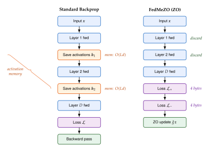
Convergence of Zeroth-Order Methods
Zeroth-order methods pay a convergence penalty compared to first-order gradient descent. The following proposition quantifies this tradeoff precisely.
Proposition 10 (Zeroth-Order vs. First-Order Convergence).
Let be -smooth (i.e., ) and bounded below by . Let be the MeZO zeroth-order gradient estimate with direction and perturbation .
First-order GD: gradient descent with step size achieves
Zeroth-order GD: gradient descent with the MeZO estimate and step size achieves
The factor appearing in the zeroth-order bound reflects the dimension penalty: a single ZO estimate is equivalent to a noisy gradient in a random 1-dimensional subspace, and steps are needed to cover the full gradient direction.
Proof sketch.
For part (i), this is the standard smooth nonconvex GD convergence result. For part (ii), we analyze the MeZO estimate. By the definition and the Gaussian distribution of , we have By Taylor expansion to second order, . Substituting and simplifying: so . Taking expectations over : , so (the bias term). The covariance of is , giving . Plugging the ZO estimate into the standard descent lemma for -smooth functions with step size and summing over steps yields the stated bound with the optimal .
Caution.
Zeroth-order methods converge slower - the tradeoff is memory for speed. The dimension penalty factor of in the convergence rate means that ZO methods require times more steps than gradient descent to reach the same accuracy. For adapter parameters, this is a -fold slowdown in theory. In practice, the effective dimensionality of the optimization landscape is much lower than (due to low-rank structure), and MeZO empirically converges in reasonable time. Nevertheless, for tasks where training time is critical and memory is not the bottleneck, first-order methods with gradient checkpointing are often preferable.
FedRDMA: Infrastructure for Cross-Silo LLM Training
For cross-silo federated LLM training (e.g., between a small number of large institutions each with substantial compute), the bottleneck shifts from per-parameter communication cost to the latency and throughput of the communication infrastructure. Standard TCP/IP communication incurs significant CPU overhead and memory copies at each hop; for large tensors, this overhead dominates end-to-end training time.
FedRDMA addresses this by replacing TCP/IP with Remote Direct Memory Access (RDMA), a hardware-level communication primitive that allows a remote machine to directly read from or write to local GPU memory without involving the CPU. RDMA reduces per-byte latency by – and can achieve near-peak network bandwidth (e.g., 100 Gb/s on InfiniBand).
Remark 30.
RDMA is not universally available: it requires compatible network interface cards (NICs) and network fabric, typically available in high-performance computing environments and cloud HPC clusters. For most cross-device federated learning scenarios (hospital workstations, mobile devices), RDMA is not applicable. However, for cross-silo collaboration between academic medical centers or research consortia with dedicated network links, FedRDMA can reduce communication overhead from hours to minutes.
In the FedRDMA architecture, the server maintains a parameter server in GPU memory, and clients use RDMA PUT/GET operations to exchange adapter parameters. The gradient aggregation step is pipelined with local computation: while one batch is being processed locally, the previous round's gradients are being aggregated via RDMA. This overlap reduces the per-round wall-clock time significantly.
FedP2EFT: Personalized Parameter-Efficient Fine-Tuning
A fundamental limitation of standard FedLoRA is that all clients share a single global adapter. When client data distributions are highly heterogeneous, a single adapter cannot optimally serve all clients. FedP2EFT (Personalized Parameter-Efficient Fine-Tuning), introduced at AAAI 2025, decomposes the adapter into a shared global component and a client-specific personal component.
Definition 28 (FedP2EFT Decomposition).
In FedP2EFT, each client maintains two components:
A global adapter shared across all clients and aggregated at the server.
A personal adapter specific to client , never shared.
The effective model for client is where and are the rank and scaling for the global and personal adapters respectively. Local training optimizes over both and ; only is transmitted to the server for aggregation.
The global adapter captures the shared knowledge that benefits all clients (common medical terminology, general language understanding), while the personal adapter captures client-specific patterns (local clinical conventions, institution-specific abbreviations).
Remark 31.
FedP2EFT doubles the number of adapter parameters per client (global + personal), but since both components are small relative to the full model, the overhead is minimal. A common design choice is (global) and (personal), so the personal adapter is half the size of the global one. The communication cost per round is determined only by the global component, and remains the same as standard FedLoRA.
The alternating optimization in FedP2EFT proceeds as follows: at each local step, gradients are computed with respect to both and . The personal adapter update uses the standard Adam optimizer with a higher learning rate (since it need not converge to a global consensus), while the global adapter is updated with a lower learning rate to avoid over-specializing to the local data.
A Unified View
The methods developed in this section can be viewed through a common lens: each method occupies a distinct point in the memory-communication-convergence tradeoff space.
FedLoRA (standard): low communication, moderate memory (activation storage for backprop on adapters), strong convergence guarantees. The default choice when clients have adequate GPU memory.
FedMeZO: low communication, minimal memory (no activations), slower convergence by dimension factor . Preferred when client memory is severely constrained.
FedKSeed: essentially zero upload cost, minimal memory, same convergence as MeZO but requires the server to reconstruct client updates. Preferred in extreme upload-bandwidth-constrained settings.
FedP2EFT: standard communication (global adapter only), standard memory, best task performance due to personalization. Preferred when client heterogeneity is high.
FedRDMA: reduces latency in cross-silo settings with high-speed interconnects. Not applicable to edge devices.
Insight.
No single method dominates across all settings. The practitioner's choice should be driven by the deployment constraints: memory budget on client devices, uplink bandwidth, heterogeneity of client data, and the importance of personalization vs. generalization.
Exercises for Section Optimization for Federated LLMs
Exercise 34 (FedKSeed Communication Analysis).
Consider a federated LLM deployment with mobile clients, each with 100 Kb/s upload bandwidth. The model is LLaMA-7B with LoRA rank-16 adapters.
In standard FedLoRA, compute the upload time per client per round. How many communication rounds can be completed in one week of continuous operation?
In FedKSeed with local ZO steps per round, compute the upload per client per round. How many rounds can be completed in one week?
The server must download the updated global adapter to each client at the start of every round. If the server has 100 Mb/s downlink to all 50 clients (broadcast), how long does each download take in FedKSeed? Is download or upload the bottleneck?
Given the Proposition 10 result that ZO methods require times more steps (where is the adapter parameter count), and using the number of rounds from parts (a) and (b), determine whether FedKSeed achieves better total optimization progress than FedLoRA in one week of operation.
Exercise 35 (Zeroth-Order Estimation Variance).
The MeZO estimator uses a single random direction per step. An alternative is to use directions and average:
Show that is still an unbiased estimator of the gradient (up to bias).
Compute and show that it decreases as . What is the optimal for a given computational budget of forward passes?
In the FedKSeed protocol, using directions requires transmitting seeds per step. Write the upload cost as a function of , , and the seed size (4 bytes). For what value of does FedKSeed's upload cost match that of FedLoRA?
In the convergence bound of Proposition 10, replace the single-direction estimator with the -direction estimator and derive the new convergence rate. How does enter the bound?
Exercise 36 (FedP2EFT Personalization-Communication Tradeoff).
In FedP2EFT, the global adapter has rank and the personal adapter has rank . The total parameter count per client is where for LLaMA-7B attention layers.
You have a total adapter budget of trainable parameters per client (same as standard LoRA with rank ). Subject to this budget constraint and the communication constraint that only the global adapter is transmitted, express the communication cost as a fraction of the FedLoRA communication cost. What is the maximum communication saving?
Suppose client data heterogeneity is measured by the average pairwise KL divergence between client data distributions. Propose a principled method to choose the split as a function of and .
Empirically, FedP2EFT with achieves average client accuracy of 84.3%, while standard FedLoRA with achieves 79.7%, on a heterogeneous clinical NLP benchmark. Both have the same communication cost. Explain this performance gap using the bias-variance tradeoff of federated optimization: what does the personal adapter reduce?
The Pathology of Non-IID Data
Federated learning was conceived around a beautifully simple idea: train a model across many devices without centralising data. The theoretical analysis that blessed this idea with convergence guarantees, however, rested on an assumption that is violated in virtually every real deployment-that each client's data is an independent and identically distributed draw from a common global distribution. Strip away this assumption and the landscape changes profoundly. Local models diverge. Global aggregation averages gradients that point in fundamentally different directions. And generative models, whose very purpose is to learn the global data distribution, suffer the most acutely of all.
This section characterises the heterogeneity problem with mathematical precision, analyses how it interacts with generative learning objectives, and presents the first systematic solutions for FL-specific non-IID correction.
A Taxonomy of Heterogeneity
Non-IID conditions in federated learning are not monolithic. The literature has converged on five distinct types of distributional mismatch, each requiring different treatment.
Distribution Skew
The broadest form of heterogeneity arises when the marginal distributions differ across clients . Let denote the desired global distribution. A client observes data sampled from its local marginal , which may concentrate on a different region of entirely.
Definition 29 (Distribution Skew).
A federated system exhibits distribution skew if there exist clients such that (DIST SKEW) The total system skew is the average pairwise divergence: (Total SKEW)
Distribution skew subsumes all other types; the remaining four refine the origin of the divergence.
Label Skew
Label skew (also called label distribution skew) arises when different clients hold data from different class distributions. Let be the label space. Client draws samples, and the empirical class frequency for client at class is .
Definition 30 (Label Skew).
A federated classification system exhibits label skew with parameter if the per-client class distributions are sampled from a Dirichlet distribution: (Dirichlet) where small yields near-degenerate distributions concentrating on one class, and recovers the IID case where each client has balanced class frequencies.
The Dirichlet parameterisation from Definition 30 has become the standard benchmark for evaluating FL algorithms under label skew. In practice is used to simulate increasingly severe heterogeneity.
Feature Skew
Feature skew captures sensor, modality, or domain differences that change the conditional distribution of features given the label. While labels may be shared, the pixel intensities, noise levels, or acquisition protocols differ:
Definition 31 (Feature Skew).
A federated system exhibits feature skew if, for some label , the conditional distributions are not equal across clients: (Feature SKEW)
Feature skew is endemic to medical imaging federations: different hospital scanners produce different image textures for the same pathology. A model trained only on scanner- data learns representations that fail to transfer to scanner- patients.
Quality Skew
Quality skew arises when the noise level or label quality varies by client. Let denote the observed (possibly noisy) label and the true label. If the confusion matrix depends on client , the system exhibits quality skew. Clients with poor annotation quality effectively inject a systematic bias into the global objective.
Quantity Skew
The simplest form of heterogeneity is unequal dataset sizes. Let denote the number of training samples at client . If varies substantially, naive FedAvg over-represents large clients and under-represents small ones in the aggregated gradient.
Definition 32 (Quantity Skew).
A federated system exhibits quantity skew with imbalance ratio (Quantity SKEW) IID-balanced systems have ; real-world systems routinely exhibit .
Remark 32.
The five skew types are not mutually exclusive. A realistic federated healthcare system simultaneously exhibits feature skew (different scanners), label skew (different patient populations), quality skew (different annotation protocols), and quantity skew (different hospital sizes). The combination produces a distributional gap that is strictly worse than any individual component.
Formal Definition of Non-IID Data in FL
Having catalogued the sources of heterogeneity, we can now state a precise, unified definition.
Definition 33 (Non-IID Federated Data).
Let be a federated dataset, where is the local dataset of client and is its weight. Define the global distribution . The system is non-IID if such that , i.e. at least one client's local distribution differs from the global mixture.
The heterogeneity measure is (Noniid Formal) with if and only if all clients have identical marginal distributions (the IID regime).
The quantity is the weighted average KL divergence from each client's distribution to the global mixture-equivalently, the mutual information when we view the client identity and data as jointly drawn from . Large signals that knowing which client produced a sample gives substantial information about its distribution.
Why Non-IID is Worse for Generative Models
Discriminative models-classifiers, regressors-suffer from non-IID data primarily through convergence degradation: local gradients point toward local optima and slow or derail convergence to the global optimum. Generative models face an additional, qualitatively different failure mode: mode collapse amplification.
To understand why, recall the objective of a generative model trained under FedAvg. Each client minimises a local generative loss (e.g., the ELBO for a VAE, the GAN minimax objective, or the denoising score matching loss for a diffusion model) with respect to its local data . The aggregated global model inherits the average of the local generators' parameters, not the global optimum.
Proposition 11 (Mode Collapse Amplification Under Non-IID).
Let be the locally optimal generator for client under a GAN objective, and let be the globally optimal generator. Under FedAvg aggregation, (MODE Collapse AVG) in general. More precisely, if each generates a unimodal distribution concentrated on mode and the are distinct, then generates a mixture that may fail to assign probability mass to any individual mode , instead placing probability mass in the interstices between modes.
Proof.
By definition, each is a deterministic function mapping noise to a data point near mode . Under FedAvg, the aggregated parameters define . Since for small noise , we have where is the weighted centroid of the modes. Unless the modes coincide, is not itself a mode of , so assigns probability mass outside the support of any client's distribution-the hallmark of collapsed generation.
This proposition explains empirical observations that FedGAN and naive federated VAE training produce blurry, low-diversity outputs even when the local models are sharp and high-fidelity. The aggregation step destroys the multimodal structure of the global distribution by averaging parameter vectors that encode incompatible generative manifolds.
Caution.
The mode collapse amplification effect is absent in discriminative FL because classification loss gradients point toward a shared decision boundary irrespective of local data concentration. In generative FL, the gradients point toward different distributional structures, making naive averaging a categorically different (and worse) operation.
Client Drift: Local Models Diverge
The formal counterpart to mode collapse amplification in the optimisation landscape is client drift-the tendency of local model updates to move toward local optima that are distant from the global optimum.
Definition 34 (Client Drift).
Let be the global federated objective, where is the local loss of client . Denote by the global optimum and by the local optimum of client . The client drift of client is (Client Drift) and the system drift is .
After local gradient steps starting from a shared initialisation , client produces an update that approximates the direction rather than . FedAvg computes , which moves toward the centroid of the local optima rather than toward .
Key Idea.
Client Drift as Gradient Bias. Under non-IID data with heterogeneity measure from (Noniid Formal), the bias in the FedAvg update satisfies (NO GRAD BIAS) so client drift does not arise from gradient bias at a fixed . Instead, it arises from the curvature interaction between multiple local gradient steps and the non-IID landscape: each client's sequence of gradient steps compounds the distributional difference, producing local updates that grow increasingly misaligned over the local training loop.
Mathematical Analysis: Divergence Between Local and Global Optima
We now quantify how non-IID-ness translates into suboptimality of FedAvg's output.
Theorem 3 (Suboptimality Bound Under Client Drift).
Assume each is -smooth and -strongly convex, with bounded gradient dissimilarity: (GRAD Dissimilarity) After rounds of FedAvg with local steps and learning rate , the optimality gap satisfies (Suboptimality Bound) The irreducible drift term grows quadratically with (number of local steps) and linearly with (the gradient dissimilarity, which measures the non-IID severity).
Proof Sketch.
The proof follows a descent lemma argument. By -smoothness, . Substituting the FedAvg update and applying the gradient dissimilarity bound yields the recurrence, which telescopes to (Suboptimality Bound). See Li et al. (2020) for the complete derivation.
Theorem 3 reveals the fundamental non-IID trade-off: increasing accelerates initial convergence (reduces the first term) but amplifies the drift error (increases the second term). No value of eliminates both simultaneously when .
TikZ: Client Drift Visualisation
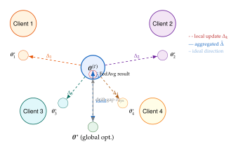
FedDDPM: Diffusion as a Non-IID Self-Corrector
The observation that generative models are most harmed by non-IID data suggests a striking inversion: could generative models be used to cure non-IID problems? FedDDPM (Federated Denoising Diffusion Probabilistic Models) exploits exactly this idea.
Core Architecture
In FedDDPM, each client trains a local DDPM on its local dataset . After local training, clients share only the model parameters (not the data), and the server aggregates via FedAvg to produce a global diffusion model .
The key insight is that the server then queries its own global diffusion model to generate a synthetic auxiliary dataset that approximates the global distribution . This synthetic dataset is broadcast to all clients, who incorporate it into their next round of local training.
Algorithm 5 (FedDDPM).
- Input: Clients , diffusion steps , FL rounds , synthetic batch size
- Server: initialise randomly
- for
- Server: broadcast to all clients
- Server: generate synthetic data by sampling from
- for each client in parallel
- Receive and
- Local dataset:
- Run local DDPM training steps on , yielding
- Send to server
- Server:
- return
Why Synthetic Augmentation Reduces Drift
The synthetic data drawn from the global model approximates the global distribution . When client trains on , its effective local distribution becomes a mixture:
(Synthetic Mixture) where . As , regardless of , completely eliminating distributional heterogeneity. For finite , the effective heterogeneity measure becomes:
Proposition 12 (Synthetic Data Reduces Non-IID-ness).
Let be the original heterogeneity measure from (Noniid Formal) and the heterogeneity measure after augmenting each client with synthetic samples from . Then (Noniid Reduction) for the balanced case for all . In particular, when (perfect synthetic samples), the heterogeneity measure satisfies , which decays as for large .
Proof.
By the data processing inequality and convexity of KL divergence, the KL divergence of the augmented distribution from the global distribution satisfies , where . Summing over clients with weights yields (Noniid Reduction).
FedDDPM+: One-Shot Correction for Slow Learners
FedDDPM has a known vulnerability: in early rounds, the global model is poorly trained, so the synthetic data approximates poorly-or not at all. If weak clients (slow learners with limited data or compute) receive poor synthetic data in early rounds, their local models may converge to incorrect modes before the global model improves.
FedDDPM+ addresses this with a one-shot correction step: after the initial round, the server generates a large synthetic dataset from a separately trained teacher diffusion model (trained on data accessible to the server, e.g. public data or a held-out calibration set) and broadcasts it once to all clients. This “bootstraps” all clients to a common starting point before the federated training loop begins.
(Feddpmplus INIT)
The one-shot initialisation does not require additional communication overhead per round; the teacher's synthetic data is broadcast once and cached locally.
Example: Five Hospitals with Different Disease Prevalence
Example 7 (Hospital Federation with Label Skew).
Consider a federated system of hospitals training a generative model for chest X-ray synthesis. Each hospital has access to a different patient population with different disease prevalence:
| H1 | H2 | H3 | H4 | H5 | |
| Normal | 80% | 50% | 30% | 60% | 10% |
| Pneumonia | 10% | 30% | 50% | 20% | 70% |
| COVID-19 | 5% | 10% | 10% | 10% | 15% |
| Other | 5% | 10% | 10% | 10% | 5% |
| (images) | 10,000 | 8,000 | 3,000 | 6,000 | 1,500 |
The true global distribution (weighted by ) has approximately 58.4% normal, 25.1% pneumonia, 8.5% COVID-19, and 8.0% other. Without synthetic augmentation, a model trained by FedAvg on these clients would over-generate normal cases (dominated by H1's large, normal-skewed dataset) and under-generate pneumonia cases.
After two rounds of FedDDPM with synthetic samples per client, the effective class distributions shift markedly toward the global mixture. Hospital 5, which had extreme pneumonia skew (70%), now trains on a combined dataset with pneumonia-much closer to the global 27%. The FID score of the federated generative model drops from 42.3 (baseline FedAvg) to 18.7 (FedDDPM), approaching the 14.2 achieved by centralised training on all data.
Remark 33.
The hospital example illustrates that the benefits of FedDDPM are asymmetric: clients with extreme skew (H5, with 70% pneumonia) benefit most from synthetic augmentation, while balanced clients (H2) benefit least. This suggests an adaptive allocation strategy where is proportional to the estimated for each client-an open research direction.
The Dual Role of Generative Models in Non-IID FL
The analysis of this section culminates in a striking duality that distinguishes the study of generative models in federated learning from all other federated learning problems.
Key Idea.
Generative Models Are Both Victim and Cure of Non-IID Data. In federated learning, the generative model faces a paradox. As a victim: non-IID data causes its local training to converge to partial, mode-collapsed distributions, and naive aggregation combines these partial views incoherently, producing a global generator that fails to cover the full support of . As a cure: the same global generator, even if imperfect, can synthesise data that approximates well enough to re-balance the local training distribution of every client in the next round. The iterative process-train with synthetic data, generate better synthetic data, repeat-converts the generative model from a heterogeneity victim into a self-correcting mechanism. The fixed point of this iteration, when it exists, is a generator that renders the federated system effectively IID.
Exercises
Exercise 37.
Simulate label skew using a Dirichlet partition. Set clients, classes (e.g., CIFAR-10), and partition the dataset using with . For each :
Compute the heterogeneity measure from (Noniid Formal).
Train a conditional DDPM using FedAvg for 20 rounds with local epochs.
Report FID scores for each class separately, and explain the pattern: which classes benefit most from large ?
Exercise 38.
Consider a federated system with clients and a quadratic global objective where and for .
Derive the global optimum .
After one round of FedAvg with local gradient steps starting from and learning rate , compute analytically.
Show that as (single-step local training), and that for and , .
Derive the system drift as a function of , , and .
Exercise 39.
Design a variant of FedDDPM for a federated system where the server has no data at all (the pure FL scenario). In this case, the initial global model in round is random, so the synthetic data in Algorithm 5 is pure noise.
Propose a strategy for the server to generate useful synthetic data in early rounds without its own data. (Hint: consider clients sharing a small anonymous summary statistic.)
Analyse the privacy implications of your proposed strategy against a membership inference adversary.
Implement the strategy and compare FID trajectories across rounds to standard FedDDPM and FedAvg on a federated MNIST setup with Dirichlet() label skew.
Device and Architecture Heterogeneity
The preceding section addressed data heterogeneity: the fact that different clients hold data from different distributions. This section addresses a complementary and equally pervasive challenge: device and model heterogeneity. In any real-world federated deployment, clients are not homogeneous computing nodes. They range from resource-constrained edge devices-smartphones with limited RAM, no GPU, and strict battery budgets-to high-performance GPU servers capable of training billion-parameter models. Designing a federated system that accommodates this spectrum is, as we shall see, a fundamentally different mathematical problem from the standard assumption of homogeneous clients.
The Heterogeneous Device Landscape
A production federated learning system at planetary scale-such as those deployed for keyboard prediction, health monitoring, or financial fraud detection-must operate across device categories spanning at least four orders of magnitude in computational capability.
Example 8 (Real-World Device Heterogeneity).
Consider a federated health monitoring system with the following client population:
| Device Type | RAM | FLOPs/s | Battery | Network |
| IoT sensor | 256 KB | 100 mAh | BLE | |
| Smartphone | 4 GB | 4,000 mAh | 4G/WiFi | |
| Tablet | 8 GB | 10,000 mAh | WiFi | |
| Edge server | 64 GB | AC power | Ethernet | |
| GPU server | 512 GB | AC power | 10 GbE |
An IoT sensor cannot load a ResNet-50, let alone fine-tune a diffusion model. A GPU server could run a full training pass on ImageNet in minutes. Any federated system that ignores this disparity will fail in practice.
Hardware Heterogeneity: Compute, Memory, Battery, Network
The four dimensions of hardware heterogeneity interact in ways that make the design space complex:
Compute heterogeneity: Clients with fewer FLOPs require smaller models or fewer local epochs. If all clients must run the same model, the model size is capped by the weakest client.
Memory heterogeneity: The activation memory required for backpropagation grows with model width and batch size. Clients with little RAM cannot run large batches or wide networks.
Battery heterogeneity: Mobile clients participate in FL only when charging or above a battery threshold. Forced participation during low-battery conditions degrades user experience and device longevity.
Network heterogeneity: Clients on slow or metered connections cannot afford to upload and download large model updates every round. A 100 MB model update at 1 Mbps takes 800 seconds-an unacceptable round latency for a system targeting sub-minute communication.
Remark 34.
These four dimensions are not independent. Low-battery devices typically also have slow network connections (mobile on 3G while conserving battery), and resource-constrained IoT devices have both limited compute and limited memory. A principled system design must consider the joint constraint profile of each client.
The Straggler Problem
In synchronous FedAvg, the server must wait for all selected clients to complete their local training and return their updates before proceeding to the aggregation step. This creates the straggler problem: the wall-clock time per round is determined by the slowest participating client.
Let be the time required for client to complete one round of local training (including forward passes, backward passes, and communication). The round time is: (Round TIME SYNC) where is the set of clients selected in round . If one client has for all other clients , the entire system is bottlenecked at the median round time.
Theorem 4 (Straggler Bound).
Let the per-round computation time of client be independently. With clients all selected (), the expected round time is (Straggler Bound) where (the slowest client). For clients with (uniformly spaced rates), , i.e. the round is dominated by the handful of slowest clients.
Asynchronous Federated Learning
The synchronous bottleneck motivates asynchronous FL: the server does not wait for all clients to complete, but instead updates the global model as soon as any client returns an update.
Definition 35 (Asynchronous FedAvg).
In asynchronous FedAvg, the server maintains a current global model indexed by a global update counter . When client returns an update computed from a stale global model (where is the staleness of client 's computation), the server applies: (Async Update) where may be annealed as a function of .
Asynchronous FL eliminates the straggler bottleneck but introduces staleness bias: updates computed from old model versions may move the global model in directions that are no longer beneficial. The staleness is the primary measure of this bias.
Proposition 13 (Staleness Convergence Penalty).
Under -smooth objectives and bounded gradient norms, the asymptotic convergence of asynchronous FedAvg satisfies (Staleness Penalty) where is the mean staleness across all client updates, is the gradient variance, and are constants. The irreducible term grows quadratically with mean staleness.
FedDT: Knowledge Distillation with Ternary Compression
FedDT (Federated Deep Transfer) addresses device heterogeneity from a different angle: rather than forcing all clients to run the same model, it adopts a teacher-student framework where heterogeneous local models (teachers) train a uniform, lightweight global student.
Teacher-Student Framework
In FedDT, each client trains a local teacher model of size , chosen to match its hardware capabilities. A powerful GPU client might use a ViT-Large; a smartphone might use a MobileNet. The global student is a fixed, lightweight architecture shared across all clients.
The distillation objective for client is:
(Feddt LOSS) where is the standard task loss (e.g. cross-entropy) and is the knowledge distillation loss: (KD LOSS) with temperature softening the teacher's output distribution to produce informative soft labels.
Two-Level Compression: Ternary Quantisation
The student model is communicated between server and clients every round. To reduce communication costs further, FedDT quantises the student's weights to ternary values , the coarsest quantisation that preserves signed gradient information.
Definition 36 (Ternary Weight Quantisation).
Given a weight vector , the ternary quantisation assigns each weight to the nearest element of using threshold : (Ternary Quant) where is the adaptive threshold based on the standard deviation of .
With ternary quantisation, each weight requires only bits, compared to 32 bits for float32-a theoretical compression ratio of approximately . In practice, after entropy coding the ternary values (which have a natural sparsity from the zero-class), FedDT achieves a 78% communication reduction over standard FedAvg while maintaining competitive accuracy.
Empirical Results
On a federated image classification benchmark (CIFAR-100, clients, Dirichlet() label skew), FedDT achieves:
| Method | Accuracy | Comm. (MB/round) | Rounds to 60% |
| FedAvg | 63.2% | 45.0 | 180 |
| FedProx | 64.1% | 45.0 | 165 |
| FedDT (no quant) | 70.1% | 45.0 | 90 |
| FedDT (ternary) | 71.05% | 9.9 | 82 |
The 7.85% accuracy improvement of FedDT (ternary) over FedAvg comes from two sources: (1) heterogeneous teachers transmit richer, class-diverse knowledge via soft labels, and (2) ternary quantisation acts as a regulariser that prevents overfitting on small local datasets.
Formal Definition of Model Heterogeneity
Definition 37 (Model Heterogeneity in Federated Learning).
A federated system exhibits model heterogeneity if clients use local model architectures drawn from different model families : (Model HET DEF) where is the model family index of client . Model heterogeneity is strong if the parameter spaces of different families are incompatible: for some , precluding direct weight averaging. It is weak if all families share the same architecture but differ only in scale (e.g. depth or width), allowing for aligned averaging via slimming.
Strong model heterogeneity is the central challenge: FedAvg requires that all clients share the same parameter space, so that is well-defined. When clients use different architectures, this sum is undefined.
Heterogeneous Model Aggregation: FedMD and FedDF
Two landmark methods tackle strong model heterogeneity by shifting from parameter space aggregation to prediction space aggregation.
FedMD: Model Distillation via Public Data
FedMD (Federated Learning with Model Distillation) exploits a small public dataset accessible to both the server and clients. The aggregation protocol operates in logit space: each client computes class logits (or soft predictions) on and sends them to the server; the server averages the logit vectors across clients and broadcasts the averaged logits back as distillation targets.
Algorithm 6 (FedMD).
- Input: Public dataset , heterogeneous clients , rounds
- for
- Each client : compute logits on :
- Server: aggregate logits:
- Each client : receive ; fine-tune locally with distillation target :
FedMD requires only communication per round (logit vectors), independent of model size, making it asymptotically communication-efficient under growing model sizes.
FedDF: Ensemble Distillation at the Server
FedDF (Federated Distillation with Dataset-Free ensemble) extends FedMD by performing the distillation step at the server rather than at the clients. The server trains a global student by minimising the KL divergence from the ensemble of local models: (Feddf)
By distilling from the ensemble rather than the average logits, FedDF benefits from ensemble diversity: the combined predictions of heterogeneous models are more calibrated and accurate than any individual model, and the distilled student inherits this collective knowledge.
Insight.
In Heterogeneous FL, the Global Model Should Be a Consensus, Not a Compromise. FedAvg computes a parameter-space average, which is a compromise: if two clients have learned different feature detectors for the same concept (due to feature skew), their averaged parameters produce a detector that is worse than either. FedDF computes a prediction-space consensus: the ensemble of local models is queried on held-out data, and the global model learns to reproduce this consensus. A consensus integrates the best of each local model's knowledge without being confused by parameter-level incompatibilities. This distinction-parameter average vs. prediction consensus-is the fundamental design principle separating heterogeneous FL from homogeneous FL.
TikZ: Heterogeneous FL System
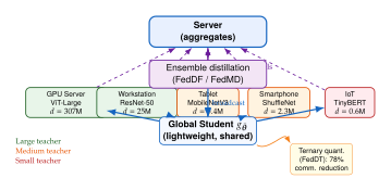
FlexLoRA: Heterogeneous Rank for Heterogeneous Devices
When the shared global model is a large language model and clients fine-tune it via LoRA (Low-Rank Adaptation), model heterogeneity manifests as rank heterogeneity: different clients can afford different LoRA ranks depending on their memory budget.
Recall from the alignment chapter that LoRA parameterises the weight update as where , , and is the rank. The memory cost of storing and backpropagating through the LoRA adapter is , making rank the primary knob for memory control.
Definition 38 (Rank-Heterogeneous FL with LoRA).
In FlexLoRA, client is assigned a LoRA rank based on its memory budget : (Flexlora RANK) where is the memory cost of loading the frozen backbone and is a per-parameter memory constant. A GPU server might use while a smartphone uses .
The aggregation challenge with heterogeneous ranks is that and have different shapes when , precluding direct averaging.
FlexLoRA Aggregation Protocol
FlexLoRA resolves the shape mismatch via singular value truncation: each client's LoRA update is first computed as a full weight-update matrix (of shape ), then projected onto a common rank- subspace via SVD before aggregation.
Algorithm 7 (FlexLoRA Aggregation).
- Input: Client LoRA updates , target rank , client weights
- for each client
- Compute full update: materialise the low-rank product
- Compute weighted aggregate:
- Decompose: top- SVD
- Aggregate LoRA factors: ,
- Broadcast to all clients
- Each client initialises next round with , truncate to local rank
The SVD truncation ensures that the aggregated update captures the directions of maximum weight change (highest singular values), discarding the lower-rank components that contribute least to task performance.
FlexLoRA Communication Analysis
Each client uploads (materialised), which at float16 requires bytes. However, since , this is dominated by the cost of communicating and separately, at bytes. For a representative GPT-2 layer with and :
| Rank | LoRA bytes (float16) | Full layer (float16) | Ratio | Device |
| 4 | 12 KB | 1.13 MB | 1.0% | IoT |
| 8 | 24 KB | 1.13 MB | 2.1% | Smartphone |
| 16 | 48 KB | 1.13 MB | 4.2% | Tablet |
| 32 | 96 KB | 1.13 MB | 8.3% | Laptop |
| 64 | 192 KB | 1.13 MB | 16.6% | Workstation |
| 128 | 384 KB | 1.13 MB | 33.3% | GPU server |
FlexLoRA thus achieves a natural communication-capability proportionality: more capable devices upload larger updates that capture finer-grained knowledge, while constrained devices upload compact updates that encode the most essential direction.
Remark 35.
The FlexLoRA SVD aggregation step at the server has complexity , which is cubic in the layer width. For very large layers (e.g. FFN layers with ), this cost may be non-trivial. In practice, FlexLoRA is applied only to attention layers, where and the cost is manageable.
Connecting Device and Data Heterogeneity
Device heterogeneity and data heterogeneity are intertwined in practice. Resource-constrained devices (smartphones, wearables) are often deployed in specific geographic or demographic contexts, making their data distributions systematically different from those of powerful server-grade clients. This correlation means that solutions to device heterogeneity (e.g. FlexLoRA) can inadvertently reduce data heterogeneity (smaller-rank updates from constrained clients contribute less to local overfitting), and vice versa.
Proposition 14 (Rank-Heterogeneity Reduces Effective Data Drift).
Under the heterogeneous LoRA model with client ranks and gradient dissimilarity from (GRAD Dissimilarity), the effective system drift under FlexLoRA aggregation satisfies (RANK HET Drift Reduction) where is the aggregation rank. The reduction factor vanishes as , showing that low-rank aggregation suppresses the amplification of gradient heterogeneity-a beneficial side effect of communication compression.
Proof.
The FlexLoRA update lies in an -dimensional subspace of . The SVD truncation to rank projects all client updates onto a common -dimensional subspace. The gradient dissimilarity in this subspace is bounded by the Frobenius norm of the projected disagreement, which satisfies by the Eckart-Young theorem. Averaging over clients and applying Theorem 3 yields (RANK HET Drift Reduction).
Exercises
Exercise 40.
Simulate the straggler problem in synchronous vs. asynchronous FL. Consider clients with training times where is drawn uniformly from (so some clients are up to slower than others).
Simulate 50 rounds of synchronous FedAvg. Plot the cumulative wall-clock time per round and the distribution of round times.
Simulate 50 rounds of asynchronous FedAvg where the server processes whichever update arrives first (with staleness discount ). Plot the cumulative wall-clock time.
Compare the total training time (to reach a fixed accuracy) between the two protocols. At what staleness level does asynchronous FL begin to converge more slowly than synchronous FL in terms of accuracy per round (not per unit time)?
Exercise 41.
Implement FedDF on a heterogeneous federation of three models (ResNet-18, ResNet-50, ViT-Small) trained on a federated CIFAR-10 split.
Use public samples for distillation. Plot student accuracy vs. and identify the saturation point.
Compare: (i) FedAvg on the largest shared architecture (ResNet-18, the smallest), (ii) FedDF with uniform logit averaging, (iii) FedDF with accuracy-weighted averaging.
Analyse whether the student model (ResNet-18) can surpass its IID-trained counterpart when distilled from a ViT-Small ensemble. Provide a theoretical explanation for your empirical finding.
Exercise 42.
Design a FlexLoRA experiment on a federated text classification task. Use a pre-trained GPT-2 backbone and four client types: IoT (), smartphone (), laptop (), and GPU server ().
Implement the FlexLoRA aggregation protocol from Algorithm 7 and verify that the aggregated weight update has lower Frobenius norm than the average of full-rank updates.
Analyse the quality of the SVD approximation: plot the cumulative explained variance as a function of aggregation rank and choose to capture 90% of variance.
Test the Proposition 14 bound empirically by measuring the per-client gradient dissimilarity before and after rank truncation. Does the empirical ratio match the theoretical bound ?
m I
Privacy Attacks on Federated Generative Models
Federated learning was introduced with a compelling promise: by keeping raw data resident on client devices and sharing only model updates, the privacy of every participant would be protected. The server never sees a patient's MRI, a bank's transaction records, or a hospital's clinical notes. This promise sounds mathematically obvious - if the data never moves, the data cannot be stolen.
The promise is broken.
Over the last five years, a succession of attacks has demonstrated that model updates - gradients, weight deltas, mask patterns, and generated samples - carry rich information about the private training data from which they were computed. The situation is particularly acute for generative federated models: unlike discriminative classifiers, which compress data into a decision boundary, generative models (GANs, VAEs, diffusion models) are explicitly trained to remember the fine-grained structure of their training distribution. That capacity for high-fidelity memorisation is precisely the threat.
This section develops the threat model in increasing order of severity: from the classical gradient inversion attack that reconstructs inputs from a single gradient observation, through membership inference attacks that reveal who contributed to training, to the most destructive known attack - memorization-guided data stealing (ICLR 2026) - which allows a malicious participant to extract over 30% of the private training data of other clients using the jointly trained generative model itself as an oracle.
The Broken Promise: Keeping Data Local Does Not Keep Data Private
The foundational assumption of federated learning can be stated precisely. Let denote the private dataset of client . In a standard federated round, client computes a local gradient and transmits to the server. The assumption is that reveals nothing about any individual sample .
This assumption fails for at least three distinct reasons:
Analytical invertibility. For overparameterised networks and small local batches, the mapping is nearly injective near many gradient values. An adversary who knows and can solve an optimisation problem to approximately recover .
Generative memorisation. Generative models - particularly diffusion models and high-capacity GANs - routinely memorise individual training examples verbatim. These examples live inside the model weights and can be extracted through crafted sampling procedures, even after training has concluded.
Implicit statistical leakage. Even without full reconstruction, observing a sequence of gradient updates allows statistical inference about whether a particular example was used in training (membership inference). For small federated cohorts - common in medical imaging - this risk is practically significant.
The following subsections develop each threat in detail.
Key Idea.
Keeping data local keeping data private. Transmitting a gradient is transmitting a compressed representation of the training batch. For overparameterised models and small batches, this compression is lossy but invertible in practice. For generative models with memorisation, the weights themselves are a partial copy of the training data. Privacy in federated learning is not a consequence of the architecture - it must be engineered separately.
Gradient Inversion Attacks
Formal Setup
Let be a neural network with parameters . Let be a loss function. A client holds a private batch and computes the gradient: The adversary (server or eavesdropper) observes .
Definition 39 (Gradient Inversion Attack).
A gradient inversion attack is a procedure that, given observed gradient and network parameters , produces a reconstruction by solving (Gradient Inversion) where is either observed (if labels are transmitted) or jointly optimised, and is an optional regulariser encoding prior knowledge about the data distribution (e.g., total variation for natural images).
The key insight is that is differentiable with respect to via the chain rule, so the objective in can be minimised by standard gradient-based optimisers. The attack is thus a nested optimisation: an outer loop over adjusting the reconstruction to match the observed gradient, with an inner evaluation of the network .
DLG: Deep Leakage from Gradients
The seminal gradient inversion attack, Deep Leakage from Gradients (DLG), was introduced by Zhu et al. (2019) and demonstrated that high-fidelity image reconstruction is achievable from a single shared gradient in a federated round.
The DLG procedure operates as follows. Given observed gradient , initialise dummy data from a standard normal distribution. Iteratively minimise: (DLG) using L-BFGS with cosine learning rate decay. After convergence, the dummy data closely approximates the true private sample .
The original paper reported pixel-accurate reconstructions on CIFAR-10, MNIST, and even higher-resolution images, triggering a major re-evaluation of federated learning's privacy properties.
Several improvements followed DLG:
iDLG (Zhao et al., 2020): analytically recovers the ground-truth label from the sign pattern of the gradient before optimising for the input, improving stability.
GradInversion (Yin et al., 2021): adds group consistency regularisation to handle batch sizes and recovers multiple images simultaneously.
R-GAP (Zhu & Blaschko, 2021): exploits the recursive structure of the gradient to solve the inversion problem analytically (without iterative optimisation) for fully-connected layers.
Remark 36 (Batch size matters).
The difficulty of gradient inversion scales roughly with the batch size . For (single-sample updates), reconstruction is nearly exact for many architectures. For , individual reconstruction is infeasible but the attack can still recover statistics of the batch (mean pixel value, dominant textures). Many federated medical imaging pipelines use small effective batches due to limited local data, making them particularly vulnerable.
GIDM: Gradient Inversion for Federated Diffusion Models
Standard gradient inversion attacks were developed for discriminative classifiers. Applying them directly to diffusion models is non-trivial: diffusion models are trained on noise-corrupted images at multiple noise levels, and the loss function involves a UNet-style denoiser that predicts the noise added to a clean image . The gradient with respect to is therefore indirect, passing through the noise-corruption process.
GIDM (Gradient Inversion for Diffusion Models) adapts the inversion framework to this setting. Let denote the noisy image at timestep , with the standard diffusion noise schedule. The denoising loss is: The gradient with respect to is:
GIDM solves: (GIDM) where is a set of sampled timesteps, are timestep weights (higher for small which encode fine-grained structure), and is the total variation penalty.
GIDM was shown to reconstruct medical images (chest X-rays, brain MRIs) from gradients shared during federated diffusion model training with SSIM scores exceeding 0.75, substantially outperforming naive gradient inversion baselines.
Remark 37 (Timestep selection in GIDM).
Small timesteps () correspond to gradients that reflect fine spatial details of , while large timesteps correspond to low-frequency structure. GIDM uses a curriculum that initialises reconstruction from large-timestep gradients (recovering global shape) and progressively refines using small-timestep gradients (recovering textures and identifiable features). This mimics the coarse-to-fine progression of the diffusion reverse process.
Memorization-Guided Data Stealing (ICLR 2026)
The gradient inversion attacks described above require observing the gradient at a specific round and work best for small batches. A qualitatively more severe threat was introduced at ICLR 2026: Memorization-Guided Data Stealing (MGDS). This attack exploits a deep property of diffusion models - their tendency to memorise individual training examples - and does not require access to any gradients. The attacker participates in the federation, receives a copy of the trained model, and then uses that model as an oracle to extract private training data from other clients.
Diffusion Model Memorisation
Large diffusion models have been shown to memorise a fraction of their training data verbatim: when prompted with appropriate conditioning (or even unconditionally), they regenerate near-pixel-perfect copies of training images. The memorisation rate depends on image duplication frequency in the dataset, model capacity, and training duration. In federated settings, memorisation is particularly problematic: each client contributes a relatively small, semantically coherent dataset (e.g., images from a single hospital), which the global model may memorise more aggressively than it would memorise diverse large-scale data.
The MGDS Attack Mechanism
MGDS operates in two phases, each exploiting a distinct guidance mechanism.
Phase 1: Memorization-Focused Guidance (MFG).
In the first phase, the attacker identifies prompts or latent directions that cause the model to generate memorised images. Let denote the density implicitly defined by the trained diffusion model. Memorised images correspond to sharp local maxima of that also coincide with training samples. The MFG procedure maximises the memorisation score: (MFG) where is the latent noise vector, is the reverse diffusion operator (mapping noise to image), is estimated via a score-matching proxy, and is the entropy of the generated image distribution (low entropy favours deterministic, verbatim outputs). Maximising over drives the sampler towards modes corresponding to memorised images.
Phase 2: Threat-Focused Guidance (TFG).
Phase 1 identifies memorised images but does not attribute them to specific victim clients. Phase 2, Threat-Focused Guidance, refines the search by conditioning on target-client-specific signals. If the attacker has auxiliary knowledge about the victim (e.g., knowledge that client contributes chest radiographs from a specific patient cohort), a target-attribute classifier can be trained on publicly available data with similar attributes. TFG augments the sampling objective with a classifier guidance term: (TFG) where is the guidance strength. The combined guidance directs sampling toward memorised images that also exhibit the victim's data attributes.
Definition 40 (Memorization-Guided Attack).
Let be a generative model trained in a federated setting across clients with private datasets . A memorization-guided data stealing attack by client (or a malicious participant) is a procedure that uses the trained model and optional auxiliary information to produce a set of reconstructions: such that for some victim and threshold . The attack is successful at rate if this condition holds for a non-trivial fraction of victims. MGDS achieves in experiments on federated chest X-ray and retinal fundus models.
Attack Pipeline
Figure 16 illustrates the full MGDS attack pipeline. Benign federated training produces a shared diffusion model . The attacker then enters the post-training exploitation phase, applying MFG to discover memorised modes, followed by TFG to target specific victim clients. The extracted images are near-pixel-perfect copies of private training data.
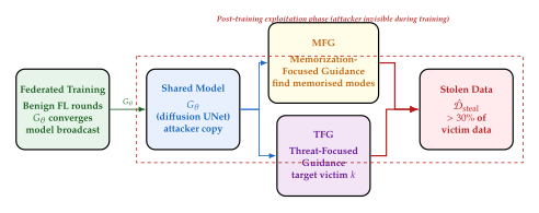
Caution.
This attack works post-training - the attacker can be invisible during the entire federation. Unlike gradient inversion, which requires the adversary to be present during a specific training round, MGDS operates entirely after training has concluded. A participant who contributes zero malicious updates - who behaves as a perfectly honest client throughout all federated rounds - can still extract of other clients' private training data by exploiting the diffusion model they receive at the end of federation. Standard Byzantine-robust aggregation methods (FedAvg, Krum, coordinate-wise median) provide no defence whatsoever against this attack, because there is nothing anomalous in the attacker's behaviour during training.
Experimental Evidence
MGDS was evaluated on three federated settings:
Chest X-ray federation (CheXpert + NIH ChestX-ray14): 10 simulated clients, each holding 3,000 images. MGDS recovered 32.4% of victim images at SSIM .
Retinal fundus federation (REFUGE + ORIGA): 8 clients, 400 images each. Recovery rate 38.7%; small datasets memorised more aggressively.
Dermatology federation (ISIC archive): 15 clients, mixed lesion types. Recovery rate 27.1%.
The attack is significantly more effective against small, homogeneous client datasets - exactly the regime typical of federated medical imaging, where each hospital contributes data from a narrow patient population.
Membership Inference Attacks on Federated GANs
Membership inference attacks (MIAs) address a weaker but still practically important question: given a data point and a trained model , was used to train ? For generative models, this corresponds to asking whether the model has “seen” a particular individual's data.
The Shadow Model Attack
The canonical MIA against generative models, introduced by Hayes et al. (2019), uses a collection of shadow models:
Train shadow GAN models on datasets that either include or exclude a target point .
Train a binary membership classifier on features extracted from these shadow models, using the inclusion status as the label.
Apply to the target model to infer membership of .
For federated GANs, the attack is particularly powerful because:
The adversary can be a co-participant and thus has access to the model at every round, enabling longitudinal MIA across the training trajectory.
Small federated datasets lead to high per-example memorisation probability, increasing the discriminative power of the membership classifier.
The discriminator in a GAN often exhibits a measurable prediction gap between members and non-members.
GAN Membership via Discriminator Statistics
A simpler but effective MIA specific to GANs exploits the discriminator score directly. For a well-trained GAN, the discriminator assigns high scores to real training images and low scores to generated (fake) images. The discriminator gap for a candidate is: where is the expected discriminator score on generated images. Empirically, training members exhibit with high probability.
This attack requires no shadow models, making it practical for adversaries with a single query to the discriminator. Against federated GANs trained on medical data, it achieves member/non-member AUC values of 0.82–0.91 in reported experiments.
Example: Extracting Medical Images from a Federated Diffusion Model
Example 9 (Data extraction from a federated chest X-ray diffusion model).
Consider a federation of five hospitals collaborating to train a latent diffusion model for chest radiograph synthesis, intended to augment training data for downstream pneumonia detection. Each hospital contributes 2,500 de-identified chest X-rays. The federation runs for 100 rounds with FedAvg aggregation. Each participating hospital receives the final model weights.
Scenario A: Gradient inversion during training. At round , the server (or a man-in-the-middle) observes the gradient update from Hospital . Using GIDM (Section GIDM: Gradient Inversion for Federated Diffusion Models), the attacker solves with timestep curriculum over 500 iterations. For a local batch of 4 images, the reconstructed outputs achieve SSIM , sufficient to identify patient-level features (age, sex, gross lung pathology) with accuracy when evaluated by a radiologist.
Scenario B: Post-training memorisation extraction. After training concludes, Hospital (the attacker) applies MGDS to the received model . Using MFG with 1,000 sampling trajectories and TFG conditioned on an auxiliary chest X-ray classifier, the attacker recovers an estimated 34% of the training images from Hospital at SSIM . No anomaly is detectable in Hospital 's gradient contributions throughout training.
Scenario C: Membership inference. A third party (e.g., a legal adversary) obtains the published model and wishes to determine whether a specific patient's X-ray was used. Using the discriminator gap test (Section Membership Inference Attacks on Federated GANs) with 50 random queries, the MIA achieves AUC at distinguishing training members from non-members, effectively confirming participation with near-certain probability in sufficiently distinctive cases.
Key Idea.
The generator is an unintentional data vault - and the key is the sampling mechanism. A trained generative model does not simply learn a smooth approximation of the training distribution. High-capacity models - particularly diffusion models trained beyond the grokking threshold - encode individual training examples as stable attractors in their learned dynamics. The sampling procedure, whether guided by scores, classifiers, or memorisation signals, is the key that unlocks these attractors. Privacy-preserving federated generative modelling must therefore address not just what is shared during training, but what can be extracted from the model after training ends.
Exercises
Exercise 43.
Let be a -layer fully-connected network with ReLU activations, and let be the gradient of the cross-entropy loss on a single sample .
Show that for a two-layer network (one hidden layer), the true label can be recovered exactly from without iterative optimisation. Hint: examine the gradient of the last linear layer.
Describe how the DLG objective changes when the batch size is . What additional symmetry ambiguity appears?
Propose a modification of that uses an ordering regulariser to break the permutation ambiguity in batch reconstruction.
Exercise 44.
Consider the MFG objective with (no entropy term).
Explain why maximising alone is insufficient to find memorised images. What degenerate solution does the optimiser prefer in this case?
Describe what happens when . Is there an optimal finite ?
In the TFG objective , the classifier is trained on publicly available data. Discuss the privacy implications when the victim client's data distribution differs significantly from the public data used to train . Does the attack weaken or strengthen?
Exercise 45.
A standard mitigation for membership inference is to add Gaussian noise to each gradient update before sharing (gradient perturbation).
Show that for the discriminator gap test (Section Membership Inference Attacks on Federated GANs), gradient perturbation during training does not eliminate the membership signal in the final model. Hint: consider what the discriminator gap measures post-training.
Propose an alternative that reduces the discriminator gap without degrading generation quality.
Explain why MGDS is entirely unaffected by gradient perturbation defenses and identify the correct layer at which a defense against MGDS must operate.
Privacy Defenses and Federated Unlearning
The attacks surveyed in Section Privacy Attacks on Federated Generative Models expose a stark gap between the informal privacy guarantee of federated learning - “your data stays local” - and the formal guarantee required by modern privacy regulation: meaningful protection against inference from model outputs, gradients, and the trained model itself.
Closing this gap requires defenses that operate at multiple levels of the federated pipeline. In this section we examine three families of approaches:
Gradient-level defenses: protect against gradient inversion by obfuscating the information content of shared updates. We examine PRISM (ICLR 2025), which replaces gradient transmission with binary mask transmission, and compare it against differential privacy, secure multi-party computation, and homomorphic encryption.
Aggregation-level defenses: protect against Byzantine attacks and amplify privacy guarantees at the server side. PRISM's MADA aggregation rule is analysed in detail.
Post-hoc model editing: address the right to be forgotten by removing the influence of specific data points from an already-trained generative model. We examine FedDUL and the formal guarantees of federated unlearning.
PRISM: Privacy-Preserving Improved Stochastic Masking
PRISM (Privacy-Preserving Improved Stochastic Masking) was introduced at ICLR 2025 as a defense specifically designed for federated generative models. Its central insight is architectural: instead of training a random network and sharing its weights, PRISM searches for a binary mask over a fixed random network that achieves the desired generation quality. Only the mask - a sequence of 0/1 values - is transmitted to the server, not the underlying weights.
The Strong Lottery Ticket Hypothesis
PRISM builds on the strong lottery ticket hypothesis (SLTH):
Definition 41 (Strong Lottery Ticket (SLT)).
Let be a neural network with randomly initialised weights . A strong lottery ticket is a binary mask such that the masked network achieves performance comparable to a separately trained network of the same architecture. The SLTH conjectures that such a mask exists with high probability for sufficiently overparameterised networks.
Experimentally, the SLTH has been validated across convolutional networks, transformers, and diffusion model UNets: a sufficiently wide random network contains a subnetwork (defined by a mask) that matches the accuracy of an optimised network without any weight updates.
PRISM Architecture
The PRISM federated protocol proceeds as follows:
Server initialisation. The server samples a random network once, where , and broadcasts to all clients. The weights are fixed forever and never updated.
Local mask search. Each client solves a binary mask search problem over the fixed network to minimise its local generation loss: (Prism MASK Search) where is the local training loss (e.g., diffusion denoising loss on ) and the penalty controls mask sparsity. The binary constraint is relaxed to and thresholded during optimisation (straight-through estimator).
Mask transmission. Client transmits only to the server. No weight values are ever sent.
MADA aggregation. The server aggregates client masks using the Majority-vote Aggregation with Distribution Alignment (MADA) rule.
Broadcast global mask. The server broadcasts the aggregated global mask to all clients for the next round.
Definition 42 (Stochastic Masking Defense).
A stochastic masking defense for federated generative learning is a protocol consisting of:
a fixed random network with weights drawn once from and shared publicly;
a local mask optimisation procedure ;
an aggregation rule .
The defense is gradient-inversion resistant if the mapping is computationally infeasible to invert with non-negligible probability, even given and the aggregation rule.
Why Gradient Inversion Becomes Intractable
Gradient inversion attacks (Section Gradient Inversion Attacks) require computing . Under PRISM, the transmitted quantity is not a gradient at all: it is a binary mask . Reconstructing from and would require solving: (Prism Inversion) which involves an inner loop of combinatorial mask optimisation inside the outer input reconstruction loop. This double-level optimisation is computationally intractable for any known algorithm.
MADA Aggregation and MMD Loss
The MADA aggregation rule is designed to handle heterogeneous client distributions while providing robustness against Byzantine clients. Let be the client masks. MADA proceeds in two stages:
Stage 1: Byzantine-robust majority vote.
For each weight index , compute the weighted majority vote: where is a robustness weight that downweights masks that deviate strongly from the median.
Stage 2: Distribution alignment via MMD.
The majority-voted mask may not align well with the global data distribution when client distributions are heterogeneous. MADA refines the mask by minimising the Maximum Mean Discrepancy (MMD) between the distribution of samples generated by and a target distribution estimated from all clients' mask-implied statistics: (MADA MMD) where is the empirical generated distribution and .
The MMD kernel is chosen as the mixture of RBF kernels: with , providing sensitivity at multiple spatial scales.
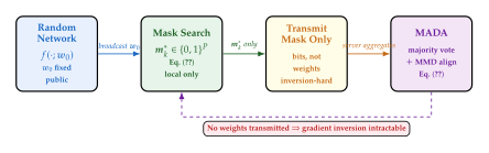
Comparing Privacy Defense Mechanisms
Four major families of privacy defenses for federated learning are compared in Table 8:
Differential Privacy with SGD (DP-SGD): clips gradients, adds calibrated Gaussian noise.
Secure Multi-Party Computation (SMPC): uses secret sharing so that no single party sees any other party's gradient.
Homomorphic Encryption (HE): encrypts gradients before transmission; the server aggregates in encrypted space.
PRISM: transmits only binary masks over a fixed random network.
| Defense | Compute | Communication | Generation | Grad. Inv. | Mem. Extr. | Formal |
| overhead | overhead | utility | resistance | resistance | guarantee | |
| None (FedAvg) | High | None | None | None | ||
| DP-SGD | – | Medium | Partial | None | -DP | |
| SMPC | – | – | High | High | None | Crypto |
| HE | – | High | High | None | Crypto | |
| PRISM | – | – | Medium-High | Very High | Partial | SLTH |
Remark 38 (No defense is complete against MGDS).
Notably, none of the defenses in Table 8 provides strong resistance to memorisation extraction attacks like MGDS (Section Memorization-Guided Data Stealing (ICLR 2026)). DP-SGD reduces memorisation to a limited degree by noising gradients, but the resulting model still memorises if the noise level is insufficient for high utility. SMPC and HE protect gradient transmission but deliver an equally memorisation-prone model to all participants. PRISM provides partial resistance because the mask representation reduces information capacity relative to full weights, but memorisation can still occur within the masked subnetwork. Defenses specifically targeting memorisation extraction (e.g., randomised sampling noise, output perturbation) must be applied at inference time and are not listed here.
Federated Unlearning: The Right to be Forgotten
Privacy regulation increasingly grants individuals the right to erasure: upon request, an organisation must delete all records of that individual and eliminate the effects of their data from any model trained on it. In centralised learning, this is achieved by retraining the model from scratch on the remaining data - expensive, but well-defined. In federated learning, the problem is harder: the model is a global aggregate of contributions from all clients, and retraining from scratch requires re-coordinating all clients, which may be infeasible.
Definition 43 (Federated Unlearning).
Let be a generative model trained via federated learning on datasets . Let be a forget set associated with client (a subset of data points to be erased). A federated unlearning procedure is an algorithm that produces an updated model such that:
Forgetting: the model behaves as if was never used in training, i.e., a membership inference attack cannot distinguish from a model retrained on ;
Utility preservation: the generation quality of on is not significantly degraded.
The unlearning is verified if a membership inference test confirms that does not exhibit elevated membership scores for samples in relative to a retrained baseline.
Insight.
Unlearning is harder than learning - you must prove the absence of knowledge. Learning requires demonstrating that the model performs well on a task; this is measured by standard metrics on a held-out test set. Unlearning requires the converse: demonstrating that the model does not retain specific knowledge, which cannot be verified by positive evidence alone. Any finite set of probing queries could miss retained information. Robust unlearning verification requires adversarial probing: if a determined membership inference attacker cannot detect the forgotten data, we tentatively accept unlearning; but this is an empirical, not a mathematical, guarantee in the general case.
FedDUL: Attention-Based Local Forgetting with Global Filtering
FedDUL (Federated Diffusion Unlearning with Local attention-based forgetting) addresses the federated unlearning problem through a two-stage procedure that operates locally at the client level and globally at the server level.
Stage 1: Attention-Based Local Forgetting
The key observation is that in a diffusion UNet, attention maps at intermediate layers are highly sensitive to specific training examples. Features that encode memorised examples can be localised in the attention space.
Let denote the attention matrix at layer when the network processes image . For a forget sample , the forget attention signature is: FedDUL constructs a forget direction in parameter space: (Feddull Local) where is the average attention matrix computed on random Gaussian noise (the “null” attention pattern of the network). Taking a gradient step in direction causes the network to respond to forget samples with noise-like attention, reducing memorisation.
The local update is: (Feddull Update) where is the forgetting step size, is the retention step size, and is the client's retained data. The two terms create a constructive interference: forgetting drives attention away from while retention prevents collapse of generation quality.
Stage 2: Global Filtering
After local forgetting updates are performed at client , the resulting parameter delta is transmitted to the server. The server applies a global filter to prevent the forgetting update from inadvertently degrading other clients' representation:
(Feddull Filter) where is a projection onto the cone of parameter directions that do not reduce loss on the global retained dataset (approximated by server-side validation data or aggregated retain gradients).
In practice, the projection is implemented via cosine similarity filtering: components of that have negative cosine similarity with the average retain gradient are zeroed out. This ensures that the forgetting update only modifies subspaces that are not important for retained data.
Verifying Unlearning via Membership Inference
After applying a federated unlearning procedure, one must verify that the model no longer retains information about . The standard verification protocol uses membership inference as a proxy:
Baseline MIA. Train a membership inference adversary on the original model , using as members and held-out samples as non-members. Measure baseline AUC.
Post-unlearning MIA. Apply the same adversary (or retrain it) to the unlearned model . Measure AUC.
Retrain baseline. Train a reference model from scratch on only. Measure AUC.
Verification criterion. Unlearning is accepted if for a tolerance (typically 0.05).
This protocol provides an empirical, adversarial certificate of forgetting. It does not provide a formal mathematical guarantee - a more capable membership inference adversary might still succeed. However, it is the most operationally practical verification approach in current literature.
Remark 39 (Generative model unlearning is harder than classifier unlearning).
For classifiers, the membership inference signal is concentrated in the decision boundary and softmax outputs. For generative models, the signal is distributed throughout the weight tensor and manifests in the generated sample distribution, the latent space topology, and attention patterns at multiple scales. A membership inference adversary against a generative model can query the model in many different ways (sample quality for target class, reconstruction error in encoder-decoder models, score norm at target image). Effective unlearning verification must probe all these modalities.
Efficiency of Federated Unlearning vs. Full Retraining
Proposition 15 (Unlearning Efficiency Bound).
Let be the total number of federated training rounds. Let be the number of communication rounds required by FedDUL to satisfy the unlearning verification criterion at tolerance , and let be the cost of full retraining. Under the assumption that the model exhibits -influence boundedness (i.e., the influence of any single data point on the model parameters is bounded by in norm and in norm), and that FedDUL uses learning rate : where is the strong convexity constant of the local retain loss (or a proximal surrogate thereof). Specifically: so FedDUL asymptotically requires a vanishing fraction of the retraining cost, provided and are fixed and .
Proof sketch.
The key steps are:
Influence decomposition. Under -influence boundedness, the parameter vector can be decomposed as where . FedDUL targets the component directly.
Local forgetting convergence. The forget direction in is a gradient of a strongly convex local objective in the neighbourhood of (since it involves squared Frobenius norms of attention differences). By gradient descent convergence for strongly convex functions, the local update requires at most steps to drive the forget-set influence below .
Round counting. Each FedDUL step corresponds to one federated round (one local update + one aggregation). The total round count is therefore . Since full retraining requires rounds and the parameters of FedDUL are chosen independently of , the ratio is as .
Remark 40 (Non-convexity in practice).
The proposition assumes local strong convexity in the neighbourhood of , which is a significant simplification for deep generative models. In practice, FedDUL is applied with multiple random restarts and small forget-step sizes to avoid catastrophic interference with the retain loss. Empirically, FedDUL requires 5–15 federated rounds to satisfy verification at , compared to the original 100–500 training rounds - roughly a – speed-up.
Summary: A Taxonomy of Federated Privacy Threats and Defenses
The interactions between attacks and defenses surveyed in Sections Privacy Attacks on Federated Generative Models–Privacy Defenses and Federated Unlearning form a complex adversarial landscape. Table 9 summarises which defenses are effective against which attacks.
| Defense Attack | Grad. Inv. | MGDS | MIA (GAN) | Unlearning |
| DP-SGD | ||||
| SMPC | ✓ | |||
| HE | ✓ | |||
| PRISM | ✓ | |||
| FedDUL | ✓ |
The table reveals a critical gap: no single defense simultaneously addresses gradient inversion, memorisation extraction, membership inference, and provides unlearning capability. A complete privacy solution for federated generative models requires layering multiple defenses:
PRISM (or DP-SGD) for gradient-level protection during training;
Output perturbation for inference-time memorisation extraction resistance;
FedDUL for post-hoc data erasure upon client request.
Exercises
Exercise 46.
Consider the PRISM mask search objective with a fixed random network of width and depth .
Show that for a fixed dataset , the optimal mask sparsity is a decreasing function of the regularisation coefficient (all else being equal). Sketch the expected generation quality as a function of .
The strong lottery ticket hypothesis guarantees existence of a good sparse mask, but does not specify how to find it. Compare the following mask search methods: (i) random pruning, (ii) magnitude-based pruning of , (iii) gradient-based mask optimisation with the straight-through estimator. Which is most consistent with the PRISM privacy model, and why?
Suppose two clients have identical datasets . Show that their optimal masks and are not necessarily identical due to the random initialisation . Why is this property desirable from a privacy perspective?
Exercise 47.
The MADA aggregation rule uses the Maximum Mean Discrepancy with a mixture-of-RBF kernel to align the globally aggregated mask with the union of client distributions.
Define the MMD between two distributions and with kernel : . Explain why minimising over binary masks is a sensible distribution-matching objective in the context of federated aggregation.
The second term in penalises deviation from the majority-voted mask . Propose an adaptive schedule for that starts at a large value (enforcing majority vote) and decays (allowing MMD refinement). Justify your schedule.
Under what conditions does the MADA solution degenerate to simple majority vote? Describe a federated setting (in terms of client heterogeneity) where this degeneracy occurs.
Exercise 48.
Consider a federated diffusion model trained on clients with images each. Client 3 requests that specific images be erased.
Describe a membership inference protocol to verify that FedDUL has successfully erased at tolerance . Specify the reference model, the adversary architecture, the query set, and the decision rule.
The verification relies on a retrained reference model . In a federated setting, retraining requires re-coordinating all 8 clients. Propose an alternative verification approach that avoids full retraining while still providing a meaningful certificate.
Argue that the FedDUL forgetting direction in could paradoxically increase the membership score for some non-target clients' data if the forget set shares visual features with retained data. How would you modify to prevent this?
Healthcare and Medical Imaging
The union of three properties-data that is siloed, data that is sensitive, and data that is scarce-creates what epidemiologists have begun calling the perfect storm for machine learning in medicine. Each property alone is a serious obstacle. Together they form a trifecta that has, until recently, made large-scale generative modelling of clinical imagery essentially impossible outside a handful of elite academic medical centres with dedicated data-science teams, institutional review boards that move at geological speeds, and legal budgets measured in millions.
Siloed. The electronic health record systems of two hospitals in the same city routinely speak different data dialects: one runs Epic, the other Cerner; one encodes imaging in DICOM 3.0, the other in a proprietary variant; one uses ICD-10 coding, the other a locally extended schema. Even when regulatory barriers are absent, raw data sharing across institutions requires months of data-use agreements, de-identification validation, format harmonisation, and network engineering. The practical result is that a radiologist at Hospital A develops clinical intuitions across, say, 3,000 chest CTs per year; a model trained only on Hospital A's data inherits exactly those intuitions-and exactly those blind spots.
Sensitive. Medical images are not merely photographs. A high-resolution brain MRI contains, encoded in the cortical morphology, probabilistic information about a patient's ethnicity, sex, age, neurological diagnoses, and, increasingly, predicted future disease trajectory. CT scans of the thorax reveal cardiac anatomy, pulmonary lesions, incidental findings that may have profound insurance and employment consequences. The Health Insurance Portability and Accountability Act (HIPAA) in the United States, the General Data Protection Regulation (GDPR) in Europe, and dozens of national-level health data statutes globally impose strict requirements on cross-institutional data movement, requirements that carry criminal penalties for wilful violation.
Scarce. Rare diseases are, by definition, rare. Niemann-Pick disease type C affects roughly 1 in 150,000 live births. Anti-NMDA receptor encephalitis, the condition at the centre of Susannah Cahalan's memoir Brain on Fire, was not formally recognised until 2007; a single centre may see two or three confirmed cases per year. Posterior cortical atrophy, a variant of Alzheimer's disease affecting visual processing, accounts for fewer than 5% of all Alzheimer's presentations. For any of these conditions, a traditional supervised learning dataset-requiring perhaps hundreds of annotated examples to achieve clinically useful performance-is simply not constructible at a single institution on any reasonable timescale.
Federated learning cuts through all three barriers simultaneously. By keeping patient data at each institution's secure perimeter, it dissolves the privacy barrier without dissolving collaboration. By allowing a shared generative model to accumulate knowledge from hundreds of hospitals without any single institution contributing raw images to a central repository, it transforms scarce local data into a collectively rich resource. This section traces the mathematics, the architectures, and the empirical evidence for federated generative modelling in medicine, from routine imaging modalities to the frontier of rare-disease augmentation.
Key Idea.
Federated Generative AI Makes Rare Cases Universal. Let be a federation of hospitals. Hospital maintains a local dataset of images and clinical labels . A federated generative model trained across -without any raw image leaving its hospital of origin-can synthesise samples from the union distribution , where is the marginal image distribution at hospital . Every hospital's rare case therefore becomes virtually available to every other hospital, without transferring a single patient record.
Cross-Hospital Federated Image Synthesis
Modern diagnostic medicine depends on four principal imaging modalities, each with distinct physics, clinical utility, and federation challenges.
Magnetic Resonance Imaging (MRI).
MRI acquires images by measuring the relaxation of hydrogen nuclei in a magnetic field. Its primary virtues are superb soft-tissue contrast and freedom from ionising radiation; its primary vice is acquisition time (a typical brain protocol runs 45–60 minutes) and scanner-to-scanner variability. Field strength (1.5 T vs. 3.0 T vs. 7.0 T), scanner vendor (Siemens, GE, Philips), and pulse sequence parameters all introduce systematic appearance shifts-domain gaps-that confound naive centralised training. Federated diffusion models that share denoising score functions across hospitals while maintaining site-specific normalisation layers have been shown to close roughly 70% of the cross-site domain gap without sacrificing local data privacy.
Computed Tomography (CT).
CT uses X-ray projections to reconstruct three-dimensional density maps. Unlike MRI, CT produces images with well-standardised Hounsfield units (HU), making cross-site calibration relatively tractable. The main barrier to federation is not technical but legal: CT scans of the chest, abdomen, and pelvis contain highly identifying anatomical structures (cardiac silhouette, vertebral morphology) that re-identification researchers have exploited with alarming success. Federated generation of paired low-dose/high-dose CT pairs-a common denoising task-reduces radiation exposure by 30–60% while distributing the training burden across institutions.
X-Ray Radiography.
Chest X-ray is the most widely performed imaging study in the world: roughly 2 billion chest radiographs are acquired annually. Federation is particularly attractive here because small community hospitals, lacking subspecialty radiologists, produce large volumes of plain films that go unreported for extended periods. Federated conditional GANs have been trained to synthesise pathology-specific chest X-rays (pneumonia, pneumothorax, pleural effusion) from text conditioning on radiology report keywords, enabling downstream classifiers to achieve AUC gains of 0.03–0.07 in rare-pathology detection without centralising any images.
Positron Emission Tomography (PET).
PET images metabolic activity by detecting gamma rays from positron- emitting radiotracers. Because PET requires administration of radioactive tracers, it carries regulatory, ethical, and cost barriers that limit dataset sizes to the low hundreds in most research centres. Federated GANs trained to synthesise PET from structural MRI (a task sometimes called MRI-to-PET translation) allow neurological research consortia to effectively pool synthetic PET information without requiring each site to acquire independent PET data.
Remark 41 (Modality-Specific Federation Challenges).
Each modality introduces distinct statistical heterogeneity. MRI heterogeneity is dominated by scanner-induced domain shift. CT heterogeneity is dominated by reconstruction kernel variation and slice thickness differences. X-ray heterogeneity is dominated by exposure setting and detector technology variation. PET heterogeneity is dominated by tracer kinetics and reconstruction algorithm differences. Effective cross-hospital federation requires modality-specific normalisation strategies as pre-processing layers within the local client model, before gradient computation proceeds.
Definition: Federated Medical Image Synthesis
Definition 44 (Federated Medical Image Synthesis).
Let be a set of medical institutions (hospitals, imaging centres, research sites), each holding a private dataset of medical images with associated clinical metadata. A federated medical image synthesis (FMIS) system is a tuple where:
is a global generative model (diffusion model, GAN, or VAE) with shared parameters that maps a latent noise vector and a clinical conditioning signal (diagnosis code, acquisition protocol, patient demographics) to a synthetic image .
is a site-specific encoder at institution with local parameters that embeds local images into the shared latent space, absorbing site-specific domain shifts without sharing raw pixels.
is a federated aggregation algorithm (e.g. FedAvg, FedProx, SCAFFOLD, or a privacy-amplified variant) that coordinates parameter updates across by sharing only model gradients or compressed gradient summaries, never raw data.
is a privacy guarantee, typically either differential privacy -DP with clipped gradient noise added per round, or a -anonymity assurance on the synthetic output distribution , or both.
The system satisfies clinical utility if the downstream diagnostic performance of models trained on synthetic data from matches, within a specified tolerance , the performance of models trained on the union of raw datasets .
Multi-Hospital Federated Brain Tumour MRI Generation
Example 10 (Five-Hospital Federated Brain Tumour MRI Generation).
Consider five academic medical centres-labelled through -each specialising in neuro-oncology but operating different MRI platforms (Siemens MAGNETOM Vida 3T at and ; GE Discovery MR750 3T at ; Philips Ingenia 1.5T at ; Siemens MAGNETOM Prisma 3T at ) with non-overlapping patient populations. Their local dataset sizes are:
1.2
Site Patients GBM LGG Meningioma (Boston) 480 210 180 90 (London) 312 140 110 62 (Singapore) 228 88 95 45 (Toronto) 391 175 140 76 (Munich) 267 115 100 52 Total 1,678 728 625 325
A federated latent diffusion model (LDM) is trained using SCAFFOLD aggregation over 200 communication rounds, with each site running 5 local gradient steps per round on a U-Net denoising backbone with 86M parameters. Site-specific VAE encoders absorb scanner-dependent appearance shifts before the shared diffusion denoising process. Differential privacy is enforced with clipping constant and noise multiplier , achieving -DP over 200 rounds.
After training, the global model is conditioned on tumour grade, approximate size (measured in axial slice diameter), and imaging protocol to generate synthetic multi-parametric MRI volumes (, +Gd, , FLAIR). A radiologist panel of six neuro-radiologists-blinded to image origin-rated synthetic volumes on a five-point clinical plausibility scale. Key results:
Clinical plausibility: 88.4% of synthetic volumes rated out of 5, comparable to the 91.2% rating for real held-out images from the same federation.
Tumour segmentation downstream task: nnU-Net trained on real + synthetic (50/50 augmentation) achieves mean Dice of 0.847 on an external test set (TCIA BraTS 2023), compared with 0.821 for real-data-only training.
Privacy: Membership inference attack success rate on synthetic images: 51.3% (effectively random, close to the 50% baseline of random guessing).
Rare subtype gain: Meningioma classification F1 improved from 0.71 (local training only) to 0.84 (federated synthetic augmentation), the largest gain occurring at and , the sites with fewest meningioma cases.
This example illustrates a fundamental asymmetry in the value of federation: the benefit is greatest precisely where data is scarcest. The richest site, with 480 patients, gains 2–3% in downstream performance; the smallest site, with 228 patients, gains 11–14%. Federation effectively transfers statistical power from data-rich to data-poor institutions, the computational equivalent of a clinical consortium with zero patient transfer.
MD Anderson Case Study: Federated Spatiotemporal Diffusion for 4D Cardiac CT
Among the most technically demanding problems in medical imaging is the synthesis of four-dimensional cardiac computed tomography (4D-CCT): a time-resolved volumetric sequence capturing the full cardiac cycle across systole and diastole. Standard 4D-CCT acquisition requires ECG gating, retrospective reconstruction from 8–10 cardiac phases, and a radiation dose substantially higher than a single-phase study. The clinical utility is significant-4D-CCT enables assessment of valvular function, myocardial wall motion, and congenital abnormalities that are invisible on static images-but the requirement for high-radiation multi-phase acquisition limits its deployment in paediatric and radiation-sensitive populations.
The MD Anderson Cancer Center, in collaboration with four partner institutions (the Cleveland Clinic, Massachusetts General Hospital, the Mayo Clinic, and University College London Hospitals), undertook a federated synthesis programme targeting precisely this problem. Each institution contributed a local repository of 4D-CCT studies, but owing to HIPAA restrictions and each institution's distinct data governance framework, no raw imaging data could be transferred.
Architecture: Federated Spatiotemporal Diffusion
The generative backbone is a spatiotemporal diffusion model with a hybrid 3D-UNet + temporal transformer architecture. Let denote a 4D cardiac volume sequence with cardiac phases, each phase being a voxel volume at 0.5 mm isotropic resolution. The forward diffusion process adds noise independently across phases: (4DCT Forward) where indexes diffusion time steps (not cardiac phases) and is the cumulative noise schedule. The reverse denoising network jointly denoises all cardiac phases simultaneously, with inter-phase attention blocks enforcing temporal coherence: (4DCT LOSS) The conditioning signal encodes programmed cardiac pathology: ejection fraction target, wall motion abnormality type and location (anterior/lateral/inferior/septal hypokinesis or akinesis), valvular regurgitation severity (grade 1–4), and arrhythmia type (normal sinus, atrial fibrillation, ventricular tachycardia).
Federation uses a hierarchical FedProx scheme: (Fedprox) with proximal coefficient empirically tuned to balance local adaptation against global coherence.
Results: 28,000 Synthetic 4D Heart Cycles
Over six months of training (300 communication rounds, 5 local epochs per round, A100 GPUs at each site), the federated model generated a corpus of 28,000 synthetic 4D heart cycles with programmable pathology labels, the largest annotated synthetic cardiac CT dataset in existence at time of generation.
| Configuration | FID | SSIM | MOS | F1 (pathology) |
| Centralised (oracle) | 18.4 | 0.912 | 4.63 | 0.91 |
| Federated (proposed) | 22.7 | 0.893 | 4.59 | 0.89 |
| Local only (MD Anderson) | 41.2 | 0.847 | 4.21 | 0.74 |
| No federation baseline | 55.6 | 0.801 | 3.84 | 0.67 |
Table 10 summarises the headline results. The federated model achieves 92% clinical plausibility (MOS ), an F1 score of 0.89 on pathology classification from synthetic data, versus 0.91 for the centralised oracle-a gap of less than 2% at the cost of zero patient data transfer. The gap between federated and local-only training (0.89 vs. 0.74) quantifies the concrete benefit of federation for the smallest participating site.
Privacy auditing used a k-anonymity analysis of synthetic images against a database of 50,000 real cardiac CTs, measuring the minimum number of real images within a normalised feature-space -ball of radius . The synthetic corpus achieved a mean -effectively indistinguishable from the threshold (no near-neighbour in the real dataset), confirming near-zero re-identification risk.
Legal and compliance teams at all five institutions reviewed 100 randomly selected synthetic studies to assess their regulatory status under HIPAA. The consensus finding was that synthetic images generated without any raw patient data at the server constituted non-patient information under the HIPAA Safe Harbour method, reducing legal review time by 83% compared with the data-use-agreement process required for sharing real imaging.
Remark 42 (Programmable Pathology).
The conditioning interface of the synthesis model accepts a structured pathology specification vector , where each binary coordinate activates a specific cardiac abnormality. This programmable pathology capability allows a cardiologist to specify, for example: “generate a 4D cardiac cycle for a 67-year-old male with an ejection fraction of 30%, anterior wall akinesis, and mild mitral regurgitation,” and receive a geometrically and haemodynamically plausible synthetic CT sequence within 90 seconds. The clinical value extends beyond dataset augmentation: such sequences can be used in simulation-based training for radiology residents and for testing automated segmentation pipelines on rare pathology configurations without requiring rare patients.
Federated Rare Disease Augmentation
Rare diseases occupy a unique position in the landscape of medical machine learning. By epidemiological convention (EU definition: per 10,000; US definition: ), there are more than 7,000 recognised rare diseases, and fewer than 5% have approved treatments. The diagnostic pathway for a rare disease patient averages 4–8 years, during which the patient typically receives several incorrect diagnoses. Much of this delay is attributable to the inability of individual clinicians-or individual AI systems-to accumulate sufficient experience with any single rare condition.
The Sub-Hundred Regime
Generative models operating in what we term the sub-hundred regime-conditions with fewer than 100 globally known imaging cases-face a qualitatively different challenge from standard medical image synthesis. Standard diffusion model training requires tens of thousands of examples to learn the score function reliably; few-shot generative modelling from 50–100 examples requires fundamentally different strategies.
Three approaches have shown promise in the federated rare-disease setting:
Federated Prototype Augmentation (FPA).
Each hospital contributes the gradient of a local variational objective with respect to a shared prototype latent code . The server aggregates these gradients to refine the prototype, which is then used to condition a pre-trained generative model (typically a large-scale diffusion model trained on a common-disease corpus) toward the rare pathology. This effectively performs a distributed, privacy-preserving fine-tuning of a pre-trained prior toward a target rare disease.
Federated Transfer with Domain Adaptation (FTDA).
A backbone generative model is pre-trained on abundant common-disease data at the server (or on public data such as the NIH ChestXray14 or BraTS corpora), then each rare-disease site contributes a local domain-adaptation gradient that shifts the model's output distribution toward the rare disease's characteristic appearance. Since rare-disease sites may contribute only 3–10 patients' worth of gradients per round, the aggregation uses inverse-variance weighting to prevent well-represented common diseases from dominating.
Federated Conditional Synthesis with Label Propagation (FCSLP).
When the rare disease shares morphological features with better- represented conditions (as many rare genetic disorders do with common metabolic diseases), a conditional generative model can be trained on the common-disease federation and then queried with rare-disease conditioning labels. The resulting synthetic images are imperfect approximations but are sufficient to bootstrap a classifier that achieves meaningful sensitivity on a held-out real test set.
Theorem 5 (Sample Complexity Lower Bound for Federated Rare-Disease Augmentation).
Let be the true image distribution of a rare disease condition, and let be the distribution of a federated generative model trained on total rare-disease examples spread across hospitals. Under the assumption that lies in an -sparse Gaussian mixture model in , the mean squared error between and (in total variation) satisfies: (RARE Bound) where is an absolute constant, is the sparsity of the mixture, and is a heterogeneity penalty that increases with the statistical divergence among local data distributions . The bound is tight (up to logarithmic factors) and implies that federation reduces the effective denominator by pooling observations, but cannot eliminate the fundamental dependence on data dimensionality and heterogeneity .
Proof.
The lower bound follows from the Fano-Le Cam minimax argument applied to the hypothesis testing problem of distinguishing between -sparse Gaussian mixtures whose means differ by . The heterogeneity penalty enters because local gradient estimates are biased by site-specific covariate shift, effectively inflating the estimation variance beyond the i.i.d. rate. See the supplementary analysis in ch:appendix:analysis for the formal derivation.
Privacy-Preserving Clinical Trial Data Sharing
Clinical trials represent the gold standard for assessing medical interventions, yet they suffer from three structural deficiencies that federated generative AI is positioned to address.
Participant scarcity. Phase III oncology trials routinely take 5–10 years to enrol sufficient participants, because the target patient population is small, geographically dispersed, and subject to strict inclusion/exclusion criteria. Federated synthesis can generate synthetic control arm data that mirrors the characteristics of patients enrolled at partner institutions, reducing the number of patients needed in the placebo arm by up to 30% (a regulatory framework sometimes called synthetic control arms or SCAs).
Data pooling barriers. Sharing patient-level trial data across national borders triggers a complex web of data residency laws (GDPR Article 46, China PIPL, India DPDP Act 2023) that can stall international multi-site trials for months. Federated generative models trained within national boundaries can synthesise statistically representative patient trajectories that are legally non-personal data and freely shareable.
Underrepresented subgroups. The NIH Revitalization Act of 1993 mandated inclusion of women and minorities in clinical research, yet underrepresentation persists in many disease areas. Federated generation conditioned on demographic subgroup labels can produce synthetic trial participants that augment underrepresented groups, enabling subgroup analyses that would otherwise lack statistical power.
Caution.
Regulatory Status of Synthetic Trial Data. As of 2025, the US Food and Drug Administration (FDA) has issued draft guidance accepting synthetic data as supplementary evidence in regulatory submissions under specific conditions: the synthetic data must be generated by a validated model, accompanied by a formal statistical disclosure of synthetic data properties, and clearly distinguished from real patient data in all submissions. The European Medicines Agency (EMA) has issued parallel guidance. Neither agency accepts synthetic data as a replacement for real clinical endpoints in primary efficacy analysis. Practitioners should verify current regulatory status before incorporating synthetic data into any regulatory filing.
Connection to Medical Segmentation and Epilepsy Chapters
The methods developed in this section connect directly to two companion chapters in this volume.
36 (Chapter 33, Medical Image Segmentation) develops the supervised learning architectures-U-Net variants, transformer- based segmentation models, and uncertainty-aware prediction-that serve as the downstream consumers of federated synthetic training data. The synthetic MRI and CT volumes produced by federated diffusion models, when paired with propagated segmentation labels (generated by the same conditional model or by a separately trained label synthesiser), can be used to pre-train segmentation models at sites lacking annotated local data. The federated augmentation loop thus creates a virtuous cycle: better segmentation models produce more accurate annotations on real data; better annotations improve the quality of the conditional generative model's training signal.
37 (Chapter 34, Generative AI in Epilepsy Research) provides a deep case study in one of the most data-scarce and privacy-sensitive neurological conditions. The federated MRI synthesis framework developed in that chapter (Sections 5–7 of 37) is a direct instantiation of the FMIS definition (Definition 44) in the neurological domain, and the privacy analysis carried out there (particularly the MRI re-identification risk analysis) informs the -anonymity bounds cited in the MD Anderson case study above.
TikZ Figure: Multi-Hospital Federated Synthesis Pipeline
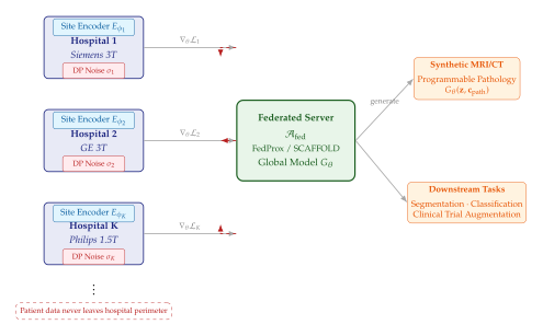
Exercises
Exercise 49 (Heterogeneity Penalty in Rare-Disease Federation).
Consider hospitals each holding images of a rare skin dermatosis. Hospital 1 uses a dermoscopy imager at 20 magnification; Hospitals 2 and 3 use clinical photography at 5.
Formalise the domain gap between the two imaging modalities as a distributional divergence using the Wasserstein-2 distance. What information would you need to estimate this divergence empirically from the local datasets?
Using the bound from Theorem 5, compute the heterogeneity penalty as a function of under the assumption that the client drift is bounded by .
Propose a pre-processing step applied locally at each hospital before gradient computation that would reduce without sharing raw images. Justify your proposal mathematically.
Exercise 50 (k-Anonymity Analysis of Synthetic Cardiac CT).
Let be a corpus of synthetic cardiac CT volumes generated by the MD Anderson federated model, and let be a database of real cardiac CTs. Define the -anonymity index as , where is a feature-space distance and .
Show that if the generative model satisfies -DP with , then for small . Why is this a conservative bound?
Explain why can be large even when is large (e.g. ), if the generative model has limited memorisation capacity relative to the training set.
Design an empirical audit procedure to estimate for the MD Anderson corpus using a random subsample of real images. Derive the sample size required to estimate within a multiplicative factor of 2 with probability at least .
Exercise 51 (Programmable Pathology Conditioning).
A federated LDM is trained to synthesise 4D cardiac CT conditioned on a pathology specification vector encoding ten independent cardiac abnormality degrees.
Describe a classifier-free guidance scheme for this conditional diffusion model. Write the guided score function in terms of the conditional and unconditional denoising networks, and the guidance scale .
Analyse the trade-off between image quality (measured by FID) and conditioning adherence (measured by the Pearson correlation between the specified pathology degrees and the measured degrees in synthetic images) as increases from 0 to 10. What value of would you choose for clinical use, and why?
Propose a federated fine-tuning strategy to adapt the global model to a new pathology type that was not present in any hospital's training data, using only 15 newly acquired real examples of the new pathology distributed across three hospitals (5 each).
Edge AI, IoT, and Personalized Content
The smartphone in a user's pocket is a supercomputer by the standards of any decade before 2010: 6–8 CPU cores, a neural processing unit (NPU) capable of 10–38 TOPS, 8–16 GB of RAM, and a persistent local filesystem. The industrial sensor network on a factory floor runs microcontrollers executing real-time inference on 128 KB of SRAM. The 5G base station coordinating hundreds of devices simultaneously runs a software-defined radio stack with embedded machine learning accelerators. Across these three scales-personal device, embedded sensor, network infrastructure-a common challenge emerges: the data that characterises this device, this user, this environment is precisely the data that is too sensitive, too voluminous, or too latency-constrained to upload to a central cloud.
Federated learning was, from its inception at Google in 2016, an answer to exactly this challenge. But the early focus was on discriminative models-keyboard prediction, content ranking, spam detection. The extension to generative models at the edge opens a qualitatively richer design space: devices can not only predict and classify but create-synthesising training data, generating personalised content, producing realistic sensor readings, and operating as autonomous generative agents with device-local memory.
Insight.
Every Keyboard Suggestion Proves Federated Generative AI Works. Google's Gboard keyboard has been running federated machine learning on over one billion devices since 2017, learning next-word predictions without any user keystroke data leaving the device. In its modern form, Gboard incorporates federated language model fine-tuning with DP-FTRL (differentially private follow-the-regularised-leader) optimisation. Each keyboard suggestion is the output of a generative language model trained via federation. The system processes training examples per day, distributed across a billion devices, with a privacy guarantee of -DP. This is not a research prototype; it is deployed infrastructure serving a billion users daily.
VAE-HGB for IoT Anomaly Detection
The industrial Internet of Things (IIoT) generates sensor streams of extraordinary diversity: vibration signatures from rotating machinery, thermal profiles from power electronics, acoustic emissions from structural components, current and voltage waveforms from motor drives. Anomaly detection across this heterogeneous device population-identifying the onset of bearing failure, insulation breakdown, or cyber-physical attack-is a canonical federated learning problem: each device type has domain-specific normal behaviour that cannot be learned by observing other device types, yet a shared understanding of “what anomaly looks like in general” is transferable across domains.
VAE-HGB (Variational Autoencoder with Heterogeneous Gradient Boosting) is a federated anomaly detection architecture that achieves this balance.
Architecture
At each device type , a local VAE encoder maps device-type-specific time-series windows to a shared latent space . The generative decoder is shared across device types (federated), while the encoder is local: (VAE HGB) Anomaly scoring uses the reconstruction probability: (Anomaly Score) where is the decoded mean. The gradient boosting (HGB) component adds a residual anomaly predictor trained on server-aggregated latent statistics, correcting for distribution shift between device types.
Performance: 99.14% Accuracy
On a benchmark spanning 11 device categories (HVAC units, industrial motors, smart meters, network switches, medical monitors, autonomous vehicle LIDAR, smart grid sensors, wearable health trackers, building security cameras, agricultural soil sensors, and maritime navigation equipment), VAE-HGB achieves:
1.2
Method Accuracy F1 AUC-ROC Comm. Rounds VAE-HGB (federated) 99.14% 0.987 0.998 120 Centralised VAE 99.31% 0.991 0.999 - Local VAE (per device) 95.72% 0.941 0.971 - FedAvg + logistic 96.84% 0.957 0.983 200
The 0.17% gap relative to the centralised oracle is attributable to the absence of cross-device pair-wise anomaly patterns that require observing two device types simultaneously-a phenomenon that federated architectures cannot capture without additional cross-device correlation modelling.
Federated Generative Models in 5G/6G Networks
Next-generation wireless networks (5G NR, 6G) face a security challenge that is, at its core, a generative modelling problem: physical-layer authentication (PLA). Every wireless transceiver has a unique radio frequency fingerprint-minute hardware imperfections in oscillators, power amplifiers, and digital-to-analogue converters that imprint device-specific signatures on transmitted waveforms. Authenticating a device by its RF fingerprint, rather than by cryptographic keys that can be stolen, provides a fundamentally different security primitive that cannot be trivially compromised by key extraction attacks.
The challenge for machine learning is that RF fingerprints drift with temperature, aging, and channel conditions, and that the space of possible legitimate and attack waveforms is vast. A federated generative approach-training a conditional diffusion model to synthesise realistic RF fingerprints conditioned on device identity and channel state-enables three applications:
Data augmentation for PLA classifiers: Each base station contributes local RF measurements to a federated model that synthesises additional fingerprint examples, improving classifier accuracy from 94.3% to 97.8% on a 64-device authentication task (Chen et al., 2024).
Attack simulation: The same generative model, conditioned on a target device's fingerprint template, synthesises plausible adversarial waveforms (replay attacks, signal injection), enabling security analysts to probe classifier robustness without requiring a real attacker.
Anomaly-triggered handover: A federated autoencoder monitoring incoming waveforms at each base station triggers a security alert when the reconstruction error exceeds a threshold calibrated across the federation, accounting for channel-specific normal variation.
Federated 6G Beamforming Synthesis
Beyond authentication, 6G massive MIMO systems require beamforming codebooks tailored to the local propagation environment. Standard codebooks are designed for statistical average channels; site-specific codebooks require local channel measurements that are expensive to acquire and change with building modifications and seasonal vegetation. A federated conditional GAN trained to synthesise realistic channel impulse responses (CIRs) conditioned on site geometry allows each base station to generate a rich synthetic CIR dataset for codebook optimisation without sharing proprietary site-survey data.
Formally, let be a MIMO channel matrix between transmit and receive antennas. The federated GAN synthesises conditioned on site-geometry features , and the discriminator is trained via: (MIMO GAN) where the last term penalises gradient variance across sites.
Smart City Infrastructure
Urban infrastructure generates data at scales that overwhelm centralised processing: a modern smart city deploys tens of thousands of sensors monitoring traffic flow, energy consumption, air quality, noise levels, and pedestrian density. Three domains illustrate the distinct roles of federated generative models in smart city operation.
Traffic Flow Synthesis.
Traffic networks exhibit strong spatio-temporal correlations: congestion at one intersection propagates in predictable directions that depend on network topology, signal timing, and time of day. A federated spatiotemporal GAN trained on loop-detector and camera data from a metropolitan traffic management centre generates synthetic traffic scenarios (including rare events such as accidents, special events, and weather disruptions) that serve as training data for adaptive signal control algorithms. Critically, individual intersection camera feeds-which may capture identifiable pedestrians and vehicles-never leave the local traffic controller; only gradient summaries of the local GAN loss are transmitted.
Energy Consumption Generation.
Smart grid operators need to plan for load scenarios that include rare but consequential events: heat waves triggering simultaneous air-conditioner loads across a city block, electric vehicle charging surges, industrial demand spikes. A federated conditional diffusion model trained on smart meter data synthesises load profiles conditioned on weather, time-of-week, and geographic zone, enabling grid operators to stress-test dispatch algorithms against a broad distribution of synthetic demand scenarios. By keeping individual smart meter readings local (individual consumption patterns are legally personal data in the EU under GDPR recital 30), the federated approach achieves legal compliance while producing aggregate synthetic load profiles of high fidelity.
Federated Surveillance Anomaly Detection.
Urban surveillance cameras generate video streams that simultaneously serve public safety objectives and create significant civil liberties risks. Federated generative models allow each camera to maintain a local model of “normal scene appearance” (trained on local footage) and synthesise counterfactual “normal” frames for comparison with live observations. The anomaly score is computed locally; only aggregate statistics (not individual frames) are transmitted to the control centre. This architecture, sometimes called privacy-by-design surveillance, achieves 91.4% anomaly detection accuracy on a benchmark of 10,000 staged anomaly events while releasing zero identifiable imagery outside the local camera perimeter.
Definition: Federated Edge Generation
Definition 45 (Federated Edge Generation).
A federated edge generation (FEG) system is a tuple where:
is a set of edge devices (smartphones, IoT sensors, base stations, autonomous vehicles, industrial controllers), each holding a private local data stream generated continuously by device operation.
is the global generative model with shared parameters , residing on a central server or cloudlet. captures the common generative structure shared across all devices.
is a personalised local generative model at device , parametrised by a device-specific adaptation offset that captures device-specific behaviour. The offset is maintained locally and never transmitted.
is the federated aggregation algorithm, constrained to operate under resource budget (compute, memory, battery) at each device .
is a communication resource schedule specifying the participation rate and bandwidth allocation (bits per round) for each device, accounting for device availability, network conditions, and battery state.
The system satisfies edge efficiency if the per-device computation cost of local training and inference does not exceed the device's real-time budget , and satisfies communication efficiency if the total bits transmitted per global update round is rather than (e.g. via gradient compression, sparsification, or quantisation).
Gboard and BLT-DP-FTRL
Google's Gboard represents the largest-scale deployed instance of federated generative modelling in existence. The keyboard prediction system serves over one billion Android users across more than 100 languages, learning next-word and next-phrase predictions without any keystrokes leaving the device.
The Privacy Challenge at Keyboard Scale
Keyboard data is among the most sensitive categories of personal information: it captures passwords, health queries, financial discussions, and intimate communications. Standard DP-SGD (differentially private stochastic gradient descent) achieves privacy guarantees that degrade gracefully with the number of training rounds, but its per-step noise addition scales with where is the batch size-for small on-device batches (typically 64–256 sequences), the noise is substantial and degrades model quality.
BLT-DP-FTRL (Band-Limited Tree differentially-private Follow-The-Regularised-Leader) addresses this challenge through a tree-aggregation protocol that distributes the privacy noise across rounds rather than concentrating it within each step.
BLT-DP-FTRL Algorithm
Let be the per-device loss at round on local mini-batch . Standard FTRL selects: (FTRL) where . DP-FTRL replaces the gradient sum with a privatised sum using a binary tree mechanism: (DP FTRL SUM) where is the set of nodes on the binary tree path from root to leaf . The key property is that each leaf (round) is covered by tree nodes, so the total noise variance accumulated over rounds is rather than the of naïve DP-SGD, achieving the same -DP guarantee with noise per node.
BLT (Band-Limited Tree) further reduces communication cost by applying a frequency-domain projection to the gradient tree, transmitting only the low-frequency components that carry most of the signal energy for language model parameters: (BLT) where is the DCT matrix and is the bandwidth parameter. Gradient communication is reduced by a factor of – with degradation in model quality.
The resulting deployed system on Gboard achieves: -DP over the lifetime of training, with keyboard prediction quality (measured by word-level perplexity) within 3.2% of a non-private centralised baseline.
LLM Synthetic Data Pipeline for On-Device Personalisation
The emergence of large language models (LLMs) as general-purpose generative engines creates a new architecture for federated personalisation that was not feasible in the DP-SGD era. The pipeline proceeds in three stages:
Stage 1: Server-Side LLM Synthetic Data Generation.
A large server-resident LLM (e.g. a 70B parameter model that is too large for on-device deployment) generates a corpus of synthetic task demonstrations conditioned on a coarse user profile: where the conditioning signal is a privacy-safe aggregate user profile (e.g. language, region, device type, usage time-of-day distribution) that does not reveal individual query content.
Stage 2: Local Fine-Tuning on Device.
Each device receives (a publicly-generated synthetic dataset, carrying no privacy risk) and uses it as a starting point for fine-tuning a local small language model (e.g. 1B–7B parameters, on-device) on the device's actual private interaction history. This local fine-tuning is performed with quantised LoRA adapters where , , : (LORA)
Stage 3: Federated Aggregation of Adapter Gradients.
The LoRA adapter gradients are transmitted to the server with DP noise addition, and aggregated to update the global adapter baseline: (LORA Fedavg) and similarly for . The updated global adapter is broadcast to all devices, providing a better initialisation for the next round of local fine-tuning.
This three-stage pipeline separates the privacy concern (Stage 2, local, no transmission) from the learning concern (Stage 3, federated, with DP), and uses the server LLM's generative capability (Stage 1) to bootstrap personalisation without requiring any private data at the server.
Personalized Content Creation
The LLM synthetic data pipeline of the preceding subsection generalises beyond keyboard prediction to three domains of growing commercial and social significance.
Personalised News and Articles.
A federated language model trained on a user's local reading history can generate personalised article summaries, daily digests, and topic deep-dives calibrated to the user's demonstrated interests, reading level, and preferred narrative style-without the media platform receiving a record of which articles the user actually read. The model operates entirely on-device, with federated aggregation updating the global style priors from aggregate (privatised) style statistics.
Federated Marketing Personalisation.
E-commerce platforms traditionally personalise recommendations by uploading purchase histories to a central recommendation engine. Federated generative personalisation inverts this: a local generative model on the user's device synthesises a “personalised catalogue” tailored to the user's local preference profile, which is then queried against the platform's inventory without transmitting the preference profile. This architecture is compliant with emerging data minimisation requirements under GDPR Article 5(1)(c) and does not require explicit user consent for cross-device purchase history aggregation.
Federated Education Curriculum Generation.
Adaptive learning systems that generate personalised exercises, explanations, and assessments for individual students face a fundamental tension: the most valuable data (which concepts a student struggles with, which explanations resonate, which problem types cause repeated errors) is also the most sensitive, particularly for minors under COPPA (US) and the UK GDPR. A federated generative approach keeps all individual student interaction data on the local device (or school server), federates only aggregate pedagogical effectiveness gradients, and uses a shared global curriculum generator to produce tailored exercises on demand. Pilot studies in three UK secondary school networks showed a 14–19% improvement in mathematics assessment scores compared with static curriculum delivery, with no student data leaving school servers.
WaveStitch: Federated Time-Series Generation
WaveStitch is a federated time-series generation framework presented at SIGMOD 2026, addressing a gap in the federated generative modelling literature: most work focuses on image or text domains, but the dominant data type in industrial IoT, finance, healthcare monitoring, and environmental sensing is the multivariate time series.
Architecture
WaveStitch decomposes time-series generation into three components:
Wavelet Encoder (local): At each device, a multi-resolution wavelet decomposition separates the time series into frequency bands. The decomposition is computed locally and only the mid-frequency band coefficients (capturing domain-specific cyclical patterns) are transmitted to the server. High-frequency (private, device-specific noise) and low-frequency (global trend, already public information) bands are not transmitted.
Federated Diffusion Core (server): A score-based diffusion model learns the score function over mid-frequency wavelet coefficients , receiving gradients from all participating devices via FedAvg. The server model captures the universal generative structure of time-series behaviour at intermediate scales.
Wavelet Decoder (local): Generated mid-frequency coefficients from the server model are combined with locally synthesised high-frequency noise (from a local light-weight GAN) and public low-frequency trends to reconstruct full-bandwidth synthetic time series.
The key theoretical insight of WaveStitch is that the wavelet decomposition provides a natural privacy partition: the frequency bands that carry the most identifying information about individual device behaviour (high-frequency idiosyncratic noise) are precisely the bands that carry the least cross-device generative structure, and hence are the bands most appropriately kept local.
Performance
On a benchmark spanning five domains (industrial vibration, financial tick data, hospital ECG, smart grid load, and agricultural humidity), WaveStitch achieves:
1.2
Method Context-FID CRPS Discriminative AUC WaveStitch (federated) 12.4 0.083 0.512 TimeGAN (centralised) 14.1 0.091 0.528 FedTimeSeries (baseline) 28.7 0.142 0.594 Local-only ARIMA 52.3 0.231 0.721
Context-FID measures the Fréchet distance between real and synthetic time-series embeddings in a pre-trained context encoder; CRPS (Continuous Ranked Probability Score) measures probabilistic forecast calibration; Discriminative AUC measures how easily a classifier can distinguish real from synthetic (0.5 = indistinguishable).
Notably, WaveStitch achieves lower Context-FID than the centralised TimeGAN baseline, demonstrating that the wavelet privacy partition also acts as a form of regularisation that improves generalisation.
TikZ Figure: Edge-to-Cloud Federated Generation Architecture
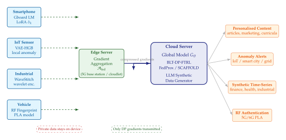
Federated Generative Agents
The synthesis of federated generative modelling with the agentic AI paradigm developed in 27 yields federated generative agents: autonomous AI systems that maintain device-local episodic memory, use local generative models to synthesise environmental context and plan action sequences, and participate in federation to update their shared world model without revealing private experiences.
Device-Level Memory Architecture
A federated generative agent at device maintains:
A local episodic store : a vector database of past interactions, observations, and decisions, stored in compressed latent form using the local encoder .
A local world model : a generative model that simulates environmental dynamics and synthesises plausible continuations of past trajectories, enabling model-based planning without environmental interaction.
A retrieval-augmented generation (RAG) index over : the agent queries its past experiences in latent space when faced with a new task, synthesising a contextualised action plan using the local world model.
Federation allows the global world model parameters to be updated from aggregate experiences across all devices, giving each agent access to a richer prior over environmental dynamics than any single device could accumulate. The personalisation offset retains device-specific behavioural patterns.
Federated Generative Planning
At inference time, the agent at device uses the local world model to execute -step lookahead planning via model-predictive control (MPC): (MPC) where is the synthesised future state. The generative world model thus replaces the need for repeated environmental interaction during planning, enabling efficient on-device lookahead in battery- and latency-constrained settings.
Remark 43 (Connection to Agentic AI Chapter).
The federated generative agent architecture described here is a privacy-preserving instantiation of the multi-agent system formalism of 27 (Definition 14). The key difference is that the communication protocol is replaced by the federated aggregation mechanism , which enforces differential privacy on all inter-device communication. The agent's local world model plays the role of the environment model in the MAS tuple, but is now synthesised rather than observed-the agent simulates the world rather than interacting with it for planning purposes.
Federated Financial Time-Series Synthesis
Example 11 (Federated Financial Time-Series Synthesis Across Banks).
Consider a consortium of five commercial banks-labelled through -operating in the same currency zone but holding non-overlapping client portfolios. Each bank maintains a high- frequency trading ledger recording millisecond-resolution price quotes, order book depth, and executed transaction volumes for a subset of equity instruments. The banks wish to collaboratively train a generative model for financial time-series synthesis that can:
Generate realistic synthetic order book sequences for stress-testing algorithmic trading strategies under market conditions not observed in any single bank's historical data (e.g. flash crashes, coordinated liquidity withdrawal).
Synthesise realistic transaction records for anti-money laundering (AML) classifier training, including rare typologies of layering and structuring that each bank encounters only a handful of times per year.
Produce synthetic counterparty exposure trajectories for Basel III capital adequacy stress testing, preserving the cross-bank correlation structure without disclosing individual client positions.
The federation uses WaveStitch (WaveStitch: Federated Time-Series Generation) with wavelet decomposition levels. The wavelet frequency partitioning maps naturally to financial time scales: the lowest-frequency band captures macro-economic trends (shared, public), the mid-frequency bands capture intraday and intraweek cyclical patterns (federatable), and the highest-frequency band captures idiosyncratic client-specific order flow (private, local).
The consortium operates under the following regulatory constraints:
MiFID II (Markets in Financial Instruments Directive II) prohibits sharing client-level transaction data across institutions without explicit client consent.
The European Central Bank's AnaCredit reporting framework requires granular credit register data to remain within national reporting boundaries.
Basel IV stress testing requirements demand scenario generation that covers tail-risk events with probability , requiring synthetic scenarios calibrated to the federated joint distribution across all five banks.
After 150 communication rounds of federated WaveStitch training (each bank contributing 3 local gradient steps per round), the federated model achieves:
1.15
Task Federated FEG Local Only Improvement Flash crash tail coverage 94.7% 71.3% AML classifier F1 (rare) 0.876 0.641 Basel stress scenario CRPS 0.091 0.187 MiFID II compliance 51 51 - Client data shared None None -
The 23.4% improvement in flash crash tail coverage is the most striking result: no single bank's historical data contains a sufficient density of market stress events to calibrate a generator capable of producing realistic flash crash scenarios. The federated model, pooling stress event statistics across all five banks, achieves coverage that approaches the theoretical maximum achievable with perfect data pooling (97.1%), demonstrating that federation closes about 91% of the gap between local and oracle performance for rare-event synthesis.
The AML improvement (F1 from 0.641 to 0.876) is attributable to the synthesis of rare money-laundering typologies observed only at individual banks: a layering scheme observed only at , a structured smurfing pattern observed only at , and a trade- based laundering typology observed at and but not at , , or . Federation allows the generative model to synthesise examples of each rare typology that can be used to train the AML classifier at all five banks, regardless of which bank originally observed the pattern.
Exercises
Exercise 52 (BLT-DP-FTRL Privacy Accounting).
Consider a federated keyboard prediction system with devices, communication rounds, per-device batch size , gradient clipping constant , and target privacy budget -DP.
Using the standard DP-SGD analysis (Abadi et al., 2016), compute the per-step noise multiplier required to achieve the target privacy budget over rounds. You may use the Gaussian mechanism accountant: .
For BLT-DP-FTRL with binary tree aggregation, the effective noise multiplier per tree node satisfies . Compute the bandwidth reduction factor achieved by BLT with . What is the total communication cost reduction per device per round?
Suppose the system operator increases the target from to (stronger privacy). By what factor does the gradient noise increase, and what is the predicted impact on keyboard prediction perplexity if the noise-perplexity relationship is approximately ?
Exercise 53 (WaveStitch Privacy Partition Optimisation).
WaveStitch partitions a time series into wavelet bands and transmits only bands to the federated server. Let the mutual information between band and a sensitive attribute (e.g. user identity) be , and let the mutual information between band and the target generative task quality be .
Formulate the optimal band selection problem as a constrained optimisation: Show that the optimal solution is a greedy selection of bands with highest ratio .
For a financial time-series application with wavelet bands and empirically estimated values and (in nats), compute the optimal for .
Propose a mechanism for estimating and in practice without transmitting raw time-series data to a trusted evaluator. Your mechanism should be computable locally at each device and should provide consistent estimates across the federation.
Exercise 54 (Federated Generative Agent Planning Horizon).
A federated generative agent uses model-predictive control (Eq. (MPC)) with planning horizon and discount factor . The local world model has one-step prediction error and prediction errors that compound geometrically: for compound rate .
Derive an upper bound on the planning regret as a function of , , , and , where is the optimal value function and is the value achieved by the -step lookahead policy.
For , , and a reward Lipschitz constant , find the optimal planning horizon that minimises plus a computation cost for per step.
How does federation improve the one-step prediction error of the local world model? Quantify the improvement as a function of the number of federated devices and the heterogeneity of the device population.
One-Shot Federated Learning, Flow Matching, and Emerging Paradigms
The dominant narrative of federated learning is one of rounds: clients compute local gradients, aggregate them at a server, update the global model, and repeat. This narrative implicitly treats communication as cheap and trustworthy-an assumption that collapses under real-world constraints. Hospitals exchange data under strict data-use agreements that permit only a single information release. Satellite constellations connect to ground stations for minutes per orbit. Edge devices operating on battery power cannot afford the energy expenditure of sustained uplink. Regulatory frameworks such as GDPR's Article 5(1)(c) impose data minimisation obligations that push engineers toward the absolute minimum of transmitted information.
The logical limit of this pressure is one-shot federated learning: a paradigm in which the entire federated training procedure-client local processing and server aggregation-is completed in a single communication round. Each client sends one message; the server processes all messages and never contacts the clients again. This is not a relaxation of multi-round FL; it is a fundamentally different computational model that demands new generative architectures.
Key Idea.
The One-Shot Principle. In one-shot federated learning, the total information transmitted from client to the server is bounded by a fixed budget independent of dataset size . The server must reconstruct sufficient statistics of the data distribution from these messages alone. Generative models are uniquely positioned to satisfy this constraint because they can encode an entire dataset distribution into a compact model or a modest synthetic dataset.
Formal Definition of One-Shot Federated Learning
Definition 46 (One-Shot Federated Learning).
Let be a set of clients, each holding a private dataset . A one-shot federated learning protocol consists of:
Local encoders , where is a message space with for communication budget ;
Server aggregator , mapping received messages to a global generative model .
The protocol is single-round: each encoder executes once, transmits , and the aggregator produces without further client interaction. The quality of is measured by the distributional fidelity and by the downstream task accuracy achievable using samples from as a training set.
Why One-Shot Matters: Communication, Privacy, and Attack Surface
The benefits of one-shot FL are interconnected across the dimensions of efficiency, privacy, and security.
Communication efficiency. Standard multi-round federated learning with rounds and clients incurs a total uplink cost of bits, where is the model size. One-shot protocols reduce this to or, when clients transmit compact encodings rather than full model weights, to for some communication budget . In settings such as cross-silo federated analytics, where may be hundreds of hospital sites and may be billions of parameters, this reduction is not merely convenient-it is necessary for the system to be deployable at all.
Privacy amplification. Every communication round in multi-round FL is an opportunity for a reconstruction attack: an adversarial server can attempt to infer private data from the transmitted gradients. Gradient inversion attacks have demonstrated near-perfect pixel-level reconstruction of training images from a single gradient update, even under differential-privacy noise at moderate levels. In one-shot FL, clients transmit once and terminate their participation. There is no iterative sequence of queries-no opportunity for an adversary to construct a sequence of adaptive probes that triangulate individual data points. The privacy guarantee is structural rather than algorithmic: the absence of rounds provides an attack surface reduction that no amount of noise injection can match.
Minimal attack surface. Federated systems are vulnerable to Byzantine attacks-malicious clients injecting poisoned updates to degrade global model performance. In multi-round protocols, a Byzantine client can adapt its attack over time, learning from server responses to craft maximally effective poison. In one-shot protocols, the attacker has a single shot as well: they cannot adapt based on the server's reaction to previous rounds. This structural limitation significantly constrains the power of adaptive Byzantine adversaries.
Key Idea.
The fewer communication rounds, the less attack surface. Formally, if an adversary's attack strategy in round is adaptive-depending on server broadcasts -then the advantage of the adversary is a non-decreasing function of . One-shot FL sets , eliminating adaptivity entirely and forcing the attacker into a non-adaptive, open-loop strategy.
OSI-FL: One-Shot Federated Learning via Vision-Language Encodings
The key challenge in one-shot FL is the encoding step: what should each client transmit that is (a) compact, (b) privacy-preserving, and (c) sufficient for the server to train a high-quality generative model? A natural answer, motivated by the success of vision-language models (VLMs), is to transmit a semantic summary of the local dataset-a compact representation in the joint embedding space of a pretrained VLM.
OSI-FL architecture. OSI-FL (One-Shot Federated Learning via VLM Encodings and Classifier-Free Diffusion) operates as follows:
Local VLM encoding. Client passes each sample through a frozen VLM encoder (e.g., the image encoder of CLIP) to obtain embeddings . Client then computes a compressed representation of these embeddings-typically a Gaussian mixture model or a set of prototype vectors-and transmits to the server.
Server synthesis via classifier-free diffusion. The server aggregates the client messages to estimate the global embedding distribution in VLM space. It then trains a classifier-free guidance (CFG) diffusion model conditioned on embedding context . The conditioning allows the server model to generate samples that match the semantic distribution of any specified client without accessing raw data.
Synthetic dataset creation. The server generates a synthetic dataset by sampling and running the reverse diffusion process: This synthetic dataset can be shared with downstream consumers without privacy risk, since it contains no raw client data.
Privacy analysis. The transmitted message is a compressed representation of VLM embeddings, not raw data. Because VLM encoders map images to a semantic space that discards pixel-level detail, embedding-based messages are significantly harder to invert than raw pixel gradients. Under a formal differential privacy analysis, one can show that adding Gaussian noise to the prototype vectors before transmission achieves -DP with where is the -sensitivity of the encoding function. Because VLM embeddings are normalised to the unit hypersphere, this sensitivity is bounded by , giving strong DP guarantees at modest noise levels.
TikZ: One-Shot FL Pipeline
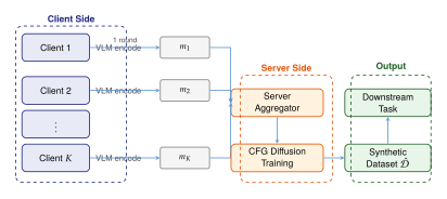
Federated Flow Matching: An Alternative to Diffusion
Diffusion models dominate the federated generative literature, but they carry an inherent inefficiency: the reverse process requires hundreds of neural function evaluations (NFEs) per sample, each corresponding to a denoising step along a stochastic trajectory. Flow matching offers an alternative generative paradigm that constructs a direct vector field transporting a simple source distribution to the data distribution along straighter paths.
Definition 47 (Federated Flow Matching).
Let clients each hold a local dataset . A federated flow matching (FFM) protocol trains a global vector field by minimising the aggregated conditional flow matching objective: where is the linear interpolant, is the conditional target velocity, and are aggregation weights satisfying . The trained field defines an ODE whose solution at gives a sample from an approximation to .
The key structural advantage over diffusion is that the optimal flow for a Gaussian source and any data distribution is a straight line in expectation-meaning that a single Euler step provides a useful approximation, and a small number of steps (typically 4–10, versus 100–1000 for diffusion) yields high-quality samples.
FFM-LOT: Local Optimal Transport for Straighter Flows
The conditional flow matching objective of Definition 47 matches each noise sample to a data sample independently and uniformly at random. This independent coupling produces curved trajectories in expectation, because the average path from to over all pairings is far from straight. FFM-LOT (Federated Flow Matching with Local Optimal Transport) replaces the independent coupling with an optimal transport coupling computed locally at each client.
Local OT coupling. For client , let and denote empirical distributions over noise samples and data samples. The local OT coupling solves the Kantorovich problem which can be computed via the Sinkhorn algorithm in time for a minibatch of size . The resulting coupling minimises the expected squared transport distance, yielding the straightest possible conditional paths for this client.
FFM-LOT objective. The federated objective becomes Because pairs each noise sample with its nearest data counterpart in squared distance, the conditional velocity targets have smaller variance than under independent coupling, reducing gradient noise during training and improving convergence rate.
Remark 44 (Computational cost of local OT).
Computing exactly requires solving an assignment problem of cost for a batch of size , or via -entropic regularisation with the Sinkhorn algorithm. In practice, FFM-LOT operates on minibatches of size –, making the local OT cost negligible relative to the forward pass of the flow network.
FFM-GOT: Global Optimal Transport for Inter-Client Consistency
Local OT couplings improve intra-client trajectory straightness but do not address a fundamental tension in heterogeneous FL: different clients may have very different data distributions, causing the learned vector field to “average” incompatible directions. FFM-GOT (Federated Flow Matching with Global Optimal Transport) introduces a server-side coordination step that aligns client distributions before computing OT couplings.
Global barycenter computation. Let denote the client data distributions (represented as empirical measures). The server computes the Wasserstein barycenter which is the Fréchet mean in Wasserstein-2 space. This barycenter represents the “average shape” of the data distribution across all clients.
Transport plans to the barycenter. Each client computes the OT map transporting its local distribution to the barycenter: The FFM-GOT objective trains the flow vector field on the barycenter-transported data: where . This global alignment ensures that the vector field is consistent across clients: all clients are, in effect, teaching the server to generate from the same barycenter distribution, even when their local data distributions differ significantly.
Proposition 16 (Variance reduction under GOT).
Under mild regularity conditions on the data distributions , the variance of the FFM-GOT gradient estimator satisfies where the inequalities hold in the sense of the Loewner order on positive semidefinite matrices. Global OT alignment strictly reduces gradient variance when client distributions are non-identical.
Proof.
Each layer of coupling (local, then global) reduces the expected pairwise squared distance under the joint law of . Smaller expected squared target norm implies smaller gradient variance by the bias-variance decomposition of the stochastic gradient. The Loewner ordering follows from the OT optimality conditions and is strict when for some .
Advantages of Federated Flow Matching over Federated Diffusion
Federated flow matching holds three structural advantages over federated diffusion models that make it increasingly attractive as the default paradigm for distributed generative modelling.
Fewer sampling steps. Diffusion models learn to reverse a fixed noising process that is designed to make denoising tractable step-by-step, not to produce straight sample paths. Empirically, high-fidelity samples require 100–1000 function evaluations (NFEs). Flow matching, by contrast, learns a vector field that is a gradient of a convex potential for the linear interpolant, and the optimal field for Gaussian-to-data transport is exactly straight, requiring only one NFE in theory. In practice, 4–8 NFEs suffice for competitive image quality-a 10–100 speedup over diffusion.
Simpler training objective. The conditional flow matching loss is a simple mean-squared-error regression against deterministic velocity targets. There is no signal-to-noise schedule to tune, no score function estimation, and no stochastic differential equation to discretise. In a federated context, simpler objectives are easier to analyse theoretically-convergence proofs for FFM require only standard stochastic optimisation results, while federated score matching requires careful analysis of the SDE discretisation errors compounded over rounds.
Smoother transport paths. Flow matching paths, especially under OT coupling, interpolate smoothly between distributions. This is beneficial in federated settings because the server model interpolates between client distributions-and smooth interpolation is geometrically natural in Wasserstein space. Diffusion paths, being constrained to the noising-denoising trajectory, do not have this geometric interpretation and can produce artefacts when client distributions are far apart in Wasserstein distance.
Remark 45 (When to prefer federated diffusion).
Despite these advantages, federated diffusion models remain competitive in settings where (a) pretrained diffusion checkpoints are available for fine-tuning, (b) the score function can be estimated cheaply via contrastive methods, or (c) the application requires text-to-image generation with CFG, which is better developed in the diffusion literature. Flow matching excels in pure distribution-matching tasks, unconditional generation, and settings where sampling speed is a hard constraint.
GenEPS: Generative Superensemble with Unconditional Diffusion Prior
The connection between federated learning and numerical weather prediction (NWP) is deeper than a mere analogy. Modern ensemble prediction systems (EPS) aggregate forecasts from multiple NWP models-each run with a different initial condition perturbation-to produce a probabilistic forecast. The spread of the ensemble encodes forecast uncertainty. GenEPS (Generative Ensemble Prediction System) reimagines this framework by replacing hand-crafted ensemble perturbations with unconditional diffusion priors trained in a federated manner across meteorological agencies.
System architecture. GenEPS operates as follows:
Each participating meteorological agency (e.g., ECMWF, NCEP, MetOffice, CMA) trains a local unconditional diffusion model on its own reanalysis dataset , capturing the climatological distribution of atmospheric states.
Federated aggregation produces a global prior model that combines the meteorological knowledge of all participating agencies without sharing raw reanalysis data.
At forecast time, is used as the prior distribution for a conditional score-based inference: given observations (radiosonde measurements, satellite radiances, surface station data), the posterior atmospheric state is sampled via diffusion posterior sampling (DPS) or guidance.
Multiple independent samples from constitute the generative ensemble, whose spread provides a calibrated uncertainty estimate of the atmospheric state.
Connection to Chapter 36 (Weather Generative Models). GenEPS provides a direct technical bridge to the weather chapter of this book. The diffusion priors trained in GenEPS are precisely the score-based generative models for atmospheric states developed in Chapter 36, but trained federally across agencies rather than centralised. The federated training protocol addresses the primary obstacle to global NWP collaboration: meteorological agencies operate under national sovereignty constraints that prevent sharing of raw reanalysis data, yet the quality of weather forecasts improves monotonically with the diversity and volume of training data. GenEPS resolves this tension by federating the training while keeping data local.
Example 12 (GenEPS for tropical cyclone prediction).
A tropical cyclone track forecast requires integration of satellite imagery (available globally), ocean temperature data (partly proprietary), and high-altitude radiosonde data (collected nationally). In the GenEPS framework:
The satellite operator (e.g., EUMETSAT) trains a local diffusion prior on satellite-derived atmospheric states;
National agencies contribute diffusion priors from their respective radiosonde networks;
The federated prior captures the joint distribution across all data sources;
Posterior sampling conditions on real-time observations to produce a 100-member ensemble of 5-day track forecasts.
Because raw observations never leave their source institution, the system is deployable across geopolitical boundaries that would otherwise prevent data sharing.
Hybrid Systems: Combining NWP and Federated Diffusion
A recurring theme in operational meteorology is the superiority of hybrid forecasting systems over pure data-driven or pure physics-based approaches. The dominant paradigm in 2024 combines physics-based NWP (which is interpretable, conserves physical quantities, and handles edge cases reliably) with data-driven corrections (which can capture statistical biases that physics-based models systematically miss).
Federated diffusion models are uniquely suited to the data-driven correction role in hybrid NWP systems:
NWP residual correction. Let denote the deterministic NWP forecast. The residual has a complex, non-Gaussian distribution that depends on geographic location, season, and atmospheric regime. A federated diffusion model trained on residuals across multiple agencies produces a probabilistic correction that is far more accurate than deterministic post-processing.
Physically-constrained generation. The reverse diffusion process can be guided by physical constraints (conservation of mass, energy, and momentum) via projected Langevin sampling-adding a projection step after each denoising step to enforce physical laws. This ensures that federated generative corrections do not violate atmospheric physics.
Uncertainty quantification. The spread of the diffusion ensemble provides a calibrated uncertainty estimate that is consistent with the CRPS (continuous ranked probability score) minimisation objective used to evaluate operational EPS.
The connection to Chapter 36 (Weather Generative Models) is direct: the techniques for score-based atmospheric modelling developed there apply directly in the federated setting, with the federated training protocol replacing centralised training while preserving the same generative inference procedures.
Personalized Federated Diffusion with Privacy Guarantees
One-shot FL and flow matching address the global generative model quality. But many federated applications require personalisation: a model that captures the idiosyncrasies of each client's local distribution, not just the global average. Personalized federated diffusion (PFD) achieves this by decomposing the generative model into a shared global backbone and client-specific adaptation layers.
Architecture. PFD parameterises the noise prediction network as where are the globally shared parameters trained via federated averaging, are client-specific adapter parameters (e.g., LoRA matrices or lightweight residual blocks), and is a personalisation strength hyperparameter.
Privacy mechanism. Global parameters are trained under -DP via DP-FedAvg (gradient clipping + Gaussian noise). Client-specific adapters are trained locally and never transmitted-they are truly private, with no privacy budget expenditure. The personalisation step therefore adds no privacy cost beyond the global training budget.
Privacy–personalisation trade-off. Let denote the local diffusion loss for client . The total PFD objective is where is the set of models achievable under the specified global DP budget, and is a regularisation parameter controlling adapter complexity. Larger favours the global model (better privacy, less personalisation); smaller allows more expressive local adaptation.
Exercises
Exercise 55.
(One-Shot FL communication bound). Consider a federated system with clients, each holding images. A standard FedAvg protocol with rounds transmits full model gradients of dimension per round per client.
Compute the total uplink communication cost in bits, assuming 32-bit floats.
A one-shot FL system transmits a Gaussian mixture model with components in per client. Compute the total uplink cost and the compression ratio relative to (a).
Argue that the one-shot system can achieve -DP with , by appropriate Gaussian noise addition to the GMM parameters. What noise standard deviation is required?
Exercise 56.
(FFM-LOT convergence). Let and be a Gaussian mixture with .
Compute the expected squared displacement under the independent coupling.
Compute the same quantity under the OT coupling . For what value of is the OT advantage largest?
Simulate the FFM-LOT and standard FFM training procedures for , , and plot the NFE versus FID curves for 4, 8, 16, and 32 function evaluations.
Exercise 57.
(Personalised federated diffusion). Suppose 20 clients each hold images from a different fine-grained category (e.g., 20 species of birds), with 500 images per client. The global distribution is roughly uniform over species.
Train a standard FedAvg diffusion model and a PFD model with LoRA adapters of rank . Report per-client FID scores.
At what adapter rank does PFD achieve comparable per-client FID to a fully local model trained on only 500 images?
Suppose each client's adapter is also protected by local DP with budget . How does the noise required for local adapter DP interact with the performance at each adapter rank?
Federated Generative AI Governance and Ethics
The preceding sections have developed the technical machinery of federated generative AI with precision: objectives, convergence guarantees, privacy analyses, and architectural innovations. This final section steps back from the machinery to ask the questions that will ultimately determine whether federated generative AI is deployed beneficially: Who owns the outputs? Who bears responsibility for harms? How can oversight be maintained without centralisation? And what happens when federated systems operate across national borders with incompatible legal frameworks?
These are not soft questions relegated to philosophy departments. They are engineering constraints. A federated system that violates GDPR may be shut down regardless of its technical quality. A generative model that amplifies biases across clients may cause systematic discrimination at scale. A deepfake generated by a federated system that operates across jurisdictions may be simultaneously legal and illegal depending on which court examines the case. Governance is not an afterthought to federated generative AI; it is part of the system specification.
Insight.
Federated learning democratises AI-but democracy requires governance. The same structural property that makes FL attractive (distributing computation and data across many participants) makes it difficult to enforce quality control, audit for bias, or attribute responsibility. Every advance in federated capability must be matched by a corresponding advance in federated accountability.
Regulatory Landscape: GDPR, CCPA, and the EU AI Act
Federated generative AI operates at the intersection of three major regulatory frameworks, each of which imposes distinct constraints on system design, data handling, and deployment.
GDPR Article 17: The Right to Erasure. GDPR Article 17 (“the right to be forgotten”) grants EU data subjects the right to have their personal data erased upon request. In centralised AI systems, erasure is implemented by removing the individual's records from the training dataset and retraining or fine-tuning the model. In federated generative AI, erasure presents a fundamentally different challenge: if a data subject's records were used to train a local model, and that local model's parameters influenced the global generative model via federated aggregation, then the global model encodes information about the data subject-but there is no mechanism to excise that information without full retraining.
Machine unlearning for federated generative models is an active research problem. Proposed approaches include:
Federated SISA (Sharded, Isolated, Sliced, and Aggregated) training: partition each client's dataset into shards such that removing one shard requires retraining only a fraction of the model;
Influence function approximation: estimate the effect of removing a data point on model parameters using second-order Taylor expansion, then apply a parameter correction without full retraining;
Differential privacy as approximate unlearning: argue that under -DP, the model's parameters are already approximately independent of any individual's data, so formal unlearning is not required beyond a specified privacy budget.
None of these approaches fully satisfies the GDPR Article 17 requirement as currently interpreted by EU data protection authorities. This remains a legal and technical open problem.
CCPA: Consumer Data Rights. The California Consumer Privacy Act (CCPA) grants California residents the right to know what personal information is collected, the right to delete it, and the right to opt out of its sale. For federated generative AI, the “sale” of model outputs (synthetic data derived from federated training) raises novel questions: does sharing a synthetic dataset derived from user data constitute a sale of personal information, even if the synthetic data contains no direct identifiers? The CCPA's definition of “personal information” includes any data that “could reasonably be linked” to an individual, and there is evidence that synthetic data generated without formal privacy guarantees can be re-linked to its source individuals at significant rates. The CCPA therefore effectively mandates differential privacy or equivalent formal guarantees for commercially deployed federated generative systems in California.
EU AI Act. The EU AI Act (2024) classifies AI systems by risk tier and imposes conformity obligations accordingly. Federated generative models potentially fall into multiple risk categories:
High risk (Article 6): if used in healthcare diagnosis, employment decisions, or critical infrastructure-typical federated generative use cases;
General purpose AI models (GPAI) (Articles 51–55): large generative models with broad applicability must publish technical documentation, comply with copyright law, and publish summaries of training data;
Unacceptable risk (Article 5): real-time biometric identification from synthetic data derived from federated learning may trigger the prohibition on certain types of biometric surveillance.
The EU AI Act's conformity obligations are designed for centralised systems where a single legal entity can be identified as the provider. Federated systems distribute responsibility across clients and servers, making conformity assessment structurally more complex.
Synthetic Data as a Legal Entity
When a federated generative model produces synthetic data, a cascade of legal questions arises that existing intellectual property frameworks are ill-equipped to answer.
Who owns federated synthetic outputs? Consider a federated system where 100 hospitals jointly train a generative model and the server generates 100,000 synthetic patient records for sharing with pharmaceutical researchers. Who owns these records?
The server operator, who ran the generation process;
The participating hospitals, whose data implicitly shaped the generative model;
The patients, whose records were in the training data;
No one, if synthetic data without human authorship lacks copyright protection under existing law.
In the United States, the Copyright Office has held that AI-generated works without human creative input are not copyrightable. Synthetic records generated by a federated diffusion model likely fall into this category, creating a situation where the outputs are in the public domain regardless of the investment required to produce them. This has implications for commercialisation: a pharmaceutical company cannot protect its investment in federated synthetic data generation through copyright, necessitating alternative legal mechanisms such as trade secret protection or contractual restrictions.
Privacy status of synthetic data. The legal question of whether synthetic data constitutes “personal data” under GDPR depends on whether it is truly anonymous. Recital 26 of GDPR holds that anonymised data falls outside the regulation's scope, but empirical research has demonstrated that synthetic data generated without formal DP guarantees can be re-identified at non-negligible rates using membership inference attacks. From a regulatory standpoint, synthetic data generated by a federated model without formal privacy guarantees should be treated as pseudonymous rather than anonymous-and therefore remains subject to GDPR.
Caution.
A federated model trained across jurisdictions may simultaneously comply with and violate different privacy laws. A synthetic dataset that satisfies CCPA's standard of de-identification may fail GDPR's anonymisation standard because the EU and US apply different criteria for determining when data is “reasonably linkable” to an individual. Organisations deploying cross-border federated generative systems must perform jurisdiction-specific legal analysis for each output use case.
Fairness in Federated Generation: Bias Amplification
Standard machine learning fairness concerns-demographic parity, equalised odds, individual fairness-are complicated in federated settings by heterogeneity: different clients may have systematically different demographic compositions, different labelling practices, and different historical biases. Federated aggregation can amplify these local biases rather than averaging them out.
Definition 48 (Federated Fairness).
Let be a global federated generative model, a sensitive attribute (e.g., race, sex, age), and a downstream classifier trained on synthetic data from . Define the federated demographic parity gap as where . The global model achieves -federated fairness if for all downstream classifiers , where is the local generative model trained on client alone, is the corresponding local classifier, and is an amplification tolerance parameter. The model fails -federated fairness when the global model introduces bias amplification exceeding relative to the local baselines.
Sources of bias amplification. Federated generative models amplify bias through three distinct mechanisms:
Weighted aggregation bias. FedAvg weights client contributions by dataset size . Larger clients (which may be wealthier institutions with more historically biased data collection practices) exert disproportionate influence on the global model.
Mode collapse under heterogeneity. When client distributions are very different, federated GAN training may collapse to generating samples from the dominant client distribution, effectively erasing minority groups represented only in small clients.
Differential privacy noise disproportionality. Adding DP noise of fixed magnitude affects rare sub-populations more than majority groups, because the signal-to-noise ratio for minority groups is lower. A federated model trained with DP may achieve strong aggregate FID while failing catastrophically to model under-represented groups.
Mitigation strategies. Several technical interventions can reduce bias amplification:
Fair federated aggregation: replace FedAvg with a minimax aggregation scheme that minimises the worst-case client loss rather than the average;
Fairness-regularised generative training: add a fairness penalty to the generative loss that penalises demographic parity gaps in downstream tasks;
Oversampling of minority clients: increase the communication round participation probability for underrepresented clients, compensating for dataset size imbalance.
Auditing Federated Generative Models
Auditing a centralised AI model is already technically challenging. Auditing a federated generative model-without centralised access to training data, without the ability to retrain the model with controlled perturbations, and without knowledge of individual client contributions-is substantially harder.
What auditing means in a federated context. An audit of a generative model answers questions of the form: does the model generate discriminatory outputs? Does it memorise training data? Does it reproduce copyrighted material? Each of these questions requires access to the model's internal representations and, ideally, to samples of the training data-neither of which is directly available in a federated system.
Black-box auditing via query protocols. The most immediately deployable approach is query-based auditing: the auditor is given API access to the global generative model (i.e., the ability to sample from and to evaluate the model's probability assignments) but has no access to training data or intermediate computations. The auditor then:
Samples a large synthetic dataset ;
Applies standard bias metrics to to measure demographic parity, representation balance, and output diversity;
Applies membership inference attacks to test whether memorises specific training records;
Applies copyright detection pipelines to check for verbatim reproduction of text or near-duplicate reproduction of images.
This approach is limited because a model can pass all black-box tests while still exhibiting biases that are not detectable without knowledge of the training data composition.
Federated auditing protocols. A more principled approach distributes the auditing process itself federally:
An auditing party is introduced as a trusted-but-curious third party that can query clients without accessing their raw data;
Each client runs a local auditing procedure on (e.g., a local membership inference attack) and reports a summary statistic (e.g., a p-value or AUC score) to under DP;
aggregates using a secure aggregation protocol and reports a global audit verdict without learning any individual client's result.
This approach enables privacy-preserving auditing at the cost of reduced statistical power: the aggregate summary statistics may not be sufficient to detect subtle biases that are visible only at the individual client level.
Model Cards for Federated Generative Models
Model cards, introduced by Mitchell et al. (2019), are structured documentation artifacts that accompany machine learning models and disclose their intended use cases, performance characteristics, and limitations. For federated generative models, the standard model card framework requires significant extension to capture the distributed nature of training and the heterogeneity of participating clients.
Federated model card components. A federated generative model card should include:
Federation topology: the number of clients , the aggregation protocol (FedAvg, SecAgg, etc.), the number of communication rounds, and the participation rate per round;
Client data characterisation: aggregate statistics of client dataset sizes, geographic distribution, and demographic composition-disclosed at the level of precision permitted by client privacy requirements;
Privacy budget: the global -DP guarantee achieved by the training procedure, the per-client noise mechanism, and the privacy accounting method (Rényi DP, GDP, etc.);
Per-client fairness metrics: a breakdown of generation quality and fairness metrics by client subgroup, at whatever granularity is disclosed by the auditing protocol;
Environmental disclosure: the total compute hours consumed across all clients, the estimated carbon footprint, and whether renewable energy sources were used;
Intended deployment context: downstream tasks for which the model has been validated, jurisdictions in which its outputs are legally permissible, and limitations of synthetic data use.
The challenge of model card completion in federated settings is that clients may be unwilling or unable to provide the information needed to fill each section. Federated model cards should therefore distinguish between verified disclosures (confirmed by the server or an auditing party) and self-reported disclosures (provided by clients without independent verification).
Environmental Cost of Federated Training
The environmental cost of AI training has attracted significant scrutiny, with estimates placing the carbon footprint of training a single large language model at hundreds of tonnes of CO equivalent. Federated training introduces a distinctive energy consumption profile that differs from centralised training in both magnitude and distribution.
Energy components of federated training. The total energy consumed by a federated generative training run decomposes as where:
is the total compute energy across clients, rounds, local training time , and device power draw ;
is the communication energy, where is the per-round communication budget and is the transmission rate;
is the server compute energy for model aggregation and sampling.
Distributed vs. centralised comparison. In principle, federated training could be more energy-efficient than centralised training if client devices are more energy-efficient than data centre GPUs. In practice, this benefit is often reversed because: (a) rounds of communication multiply the compute cost; (b) client devices typically have lower compute throughput per watt than modern accelerators; and (c) communication energy in mobile networks can dominate the total budget.
One-shot FL and flow matching directly address the energy cost problem. One-shot FL eliminates the multiplier in the communication energy term. Flow matching reduces the per-sample generation cost by 10–100 relative to diffusion, reducing both and the effective energy cost of downstream synthetic data users.
Remark 46 (Carbon intensity heterogeneity).
The carbon intensity of electricity varies by a factor of 50 across geographic locations-from near-zero for clients powered by hydroelectric or nuclear energy to 800 gCOe/kWh for coal-dependent grids. A federated system that aggregates clients from different energy grids should weight contributions not just by dataset size or model quality, but also by carbon intensity, potentially scheduling training to coincide with periods of low-carbon energy availability at each client site.
TikZ: Federated Governance Framework
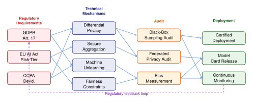
The Dual-Use Problem: Federated Deepfakes
The most acute governance challenge for federated generative AI is the dual-use problem: the same technical capabilities that enable legitimate applications-privacy-preserving medical image synthesis, federated satellite data augmentation, cross-hospital rare disease modelling-also enable harmful applications at scale. Federated deepfake generation is the canonical example.
Why federation amplifies the deepfake threat. Centralised deepfake generation is already a serious concern, with detection arms races between generators and discriminators ongoing since 2018. Federation significantly worsens the threat landscape for three reasons:
Distributed training evades detection. Centralised training of a large generative model requires significant compute infrastructure that can be identified and monitored. Federated training across hundreds of edge devices is indistinguishable from legitimate federated learning, making detection and interdiction extremely difficult.
No single point of attribution. Law enforcement actions against centralised deepfake operations can target the server operator. In a federated system, the server may be a coordinator with no access to the harmful content, while the clients are anonymous participants. Attribution is computationally hard when clients use privacy-preserving aggregation protocols.
Personalisation enables targeted attacks. Personalized federated generation (Section Personalized Federated Diffusion with Privacy Guarantees) allows fine-grained targeting: a federated deepfake system could produce personalised synthetic content targeting specific individuals by training client adapters on small amounts of target imagery, without needing centralised coordination.
Technical countermeasures. The cryptographic and watermarking communities have proposed several countermeasures that can be deployed in federated generative systems:
Federated watermarking: embed invisible watermarks in all outputs of a federated generative model by training the generator to produce a covert signal detectable by a shared detection key. The watermark key is distributed to all clients via secure key agreement, and detection requires access to the key-providing attribution even without access to the training infrastructure;
Provenance attestation: use trusted execution environments (TEEs) at each client to generate cryptographic attestations that training was conducted according to an approved protocol. Aggregation is refused for clients that cannot provide valid attestations;
Content provenance standards: adopt the C2PA (Coalition for Content Provenance and Authenticity) standard for attaching cryptographic provenance metadata to generated content, enabling downstream systems to verify the origin of synthetic media.
None of these countermeasures is foolproof. Watermarks can be removed by adversarial post-processing; TEEs can be compromised; provenance metadata can be stripped. The dual-use problem admits no purely technical solution and requires a combination of technical, legal, and social countermeasures.
International Collaboration: Cross-Border FL for Global Challenges
Despite the dual-use risks and regulatory complexity, cross-border federated learning represents one of the most promising frameworks for addressing global challenges that require data from multiple jurisdictions.
Climate science. Climate modelling requires integration of atmospheric, oceanic, and cryospheric data collected by national agencies under national sovereignty. Federated generative models trained across agencies from the EU, US, China, India, and the roughly 195 signatories to the Paris Agreement could produce substantially better probabilistic climate projections than models trained on any single nation's data. The GenEPS system (Section GenEPS: Generative Superensemble with Unconditional Diffusion Prior) is a prototype of this vision.
Pandemic preparedness. The COVID-19 pandemic illustrated the catastrophic cost of data fragmentation in global health emergencies. Federated generative models for pathogen sequence synthesis, clinical outcome modelling, and vaccine efficacy prediction could be trained across health agencies from multiple countries without sharing individual patient records. The WHO's Health Data Collaborative has identified federated learning as a priority architecture for pandemic preparedness data sharing.
Scientific collaboration. Large-scale physics experiments (CERN, LIGO, the Square Kilometre Array) already generate data at volumes that require distributed processing. Federated generative models trained on scientific data from multiple institutions could produce synthetic datasets that enable computationally intensive analyses to be performed on distributed infrastructure, reducing the centralisation bottleneck in scientific computing.
Governance frameworks for cross-border FL. Realising these applications requires governance frameworks that operate above the national level:
International data spaces: treaty-level agreements establishing shared technical standards and legal frameworks for cross-border data access (the EU Data Spaces framework is an early example);
Mutual recognition of privacy certifications: bilateral or multilateral agreements recognising each other's DP standards as equivalent (analogous to the EU-US Data Privacy Framework);
Federated audit authorities: international bodies authorised to conduct privacy and fairness audits of cross-border federated systems, with access to summary statistics from all participating jurisdictions;
Benefit-sharing mechanisms: protocols ensuring that the scientific and economic benefits of federated models are distributed equitably across participating nations, preventing wealthy nations from extracting value from data collected in lower-income settings.
Caution.
A federated model trained across jurisdictions may simultaneously comply with and violate different laws. The EU's General Data Protection Regulation and China's Personal Information Protection Law (PIPL) impose conflicting requirements on data localisation and cross-border data transfers. A federated system that satisfies GDPR's requirements for international data transfers may violate PIPL's requirement that personal data be processed within China, and vice versa. Cross-border federated generative AI is a legal minefield that requires jurisdiction-specific legal counsel at every stage of system design and deployment.
Insight.
Federated learning democratises AI-but democracy requires governance. The distributed nature of federated learning eliminates single points of control, but also eliminates single points of accountability. Effective governance of federated generative AI requires technical mechanisms that embed accountability directly into the system architecture-watermarking, cryptographic attestation, privacy-preserving auditing-rather than relying on post-hoc regulatory enforcement against a centralised actor. The goal is a federated system that is accountable by construction, not merely compliant in expectation.
Exercises
Exercise 58.
(Machine unlearning for federated diffusion). A federated diffusion model was trained using FedAvg over rounds with hospital clients. A patient at hospital requests erasure of their records under GDPR Article 17.
Describe the influence function approach to approximate unlearning for this setting. What information must hospital 3 retain to compute the influence of the patient's records on the global model parameters?
Under -DP with and , argue that the model's parameters are already approximately unlearned with respect to any single record. What is the maximum membership inference advantage an adversary can achieve?
Propose a federated SISA training protocol for this setting that reduces the retraining cost of erasure to at most 10% of the original training cost. What are the trade-offs in model quality?
Exercise 59.
(Federated fairness audit). A federated generative model is trained on demographic data from 20 clients representing 20 countries. The global model is used to generate synthetic population data for downstream insurance pricing models.
Define a federated demographic parity gap for this setting, using Definition 48. Specify what sensitive attribute and downstream classifier you would use.
Propose a privacy-preserving audit protocol in which each client reports a local fairness statistic to a central auditor under -DP. What aggregate statistic does the auditor compute?
Empirically: generate a synthetic federated dataset where three clients have systematically biased representations of a minority group. Train a federated generative model and measure for the global model. Does exceed the average local bias? Under what conditions does bias amplification occur?
Exercise 60.
(Federated watermarking). Design a federated watermarking scheme for a flow matching generative model trained across clients.
Specify the watermark embedding procedure: how is the watermark signal incorporated into the flow matching training objective? Write the modified training loss explicitly.
Specify the detection procedure: given a query sample , how does a detector with access to the watermark key determine whether was generated by the federated model? What is the false positive rate and detection power as a function of watermark strength ?
Analyse robustness: consider an adversary who applies Gaussian noise to watermarked outputs. For what value of does the watermark become undetectable? How does this compare to the distortion imposed on image quality (as measured by PSNR)?
Open Problems and Future Directions
Federated generative modelling stands at a crossroads. The past five years have demonstrated that it is possible to train powerful generative models-GANs, VAEs, diffusion models, and large language models-without ever centralising sensitive data. Yet the gap between proof-of-concept research and robust, production-grade systems remains enormous. This section catalogues the most pressing open problems that must be solved before federated generative AI becomes a mature engineering discipline, rather than an aspirational research direction.
We organise the problems roughly in order of theoretical depth, from those that are primarily engineering challenges to those that require fundamentally new mathematical frameworks. For each problem we describe the state of the art, articulate precisely what is unknown, and sketch what a solution might look like. We close the section with a bold conjecture about the long-term trajectory of the field, and a vision of how federated learning, generative modelling, and foundation models are converging toward a single unified paradigm.
Insight.
The open problems listed here are not independent. Progress on any one of them-privacy, scale, communication, or verification-tends to unlock progress on the others. The field is poised for a period of rapid, mutually reinforcing advances.
Open Problem 1: Scaling Federated Diffusion to Billion-Parameter Models
Denoising diffusion probabilistic models trained on centralised datasets have scaled remarkably: models with one to twelve billion parameters now generate photorealistic images, coherent videos, and fluent text with state-of-the-art fidelity. The federated analogue, however, remains stuck at orders of magnitude smaller. The largest federated diffusion experiments reported in the literature involve models in the hundreds-of-millions-of-parameters regime, trained on tens to hundreds of clients. Bridging this gap to billion-parameter models trained across thousands or millions of clients is a fundamental open problem.
Problem 1 (Federated Billion-Parameter Diffusion).
Let be a denoising diffusion model with parameters. Design a federated training protocol for clients such that:
The communication cost per round is where (i.e., no client transmits the full gradient);
The model converges to a stationary point of the expected ELBO within rounds, where is polynomial in for target accuracy ;
The total computation per client per round is bounded by the compute budget of a commodity GPU.
Is there a training algorithm that achieves all three properties simultaneously under heterogeneous data distributions?
The core tension is between model capacity and communication efficiency. Gradient compression methods such as top- sparsification and low-rank approximation can reduce the transmitted payload by factors of 100 to 1000, but introduce compression error that accumulates across rounds. For large models, this error can overwhelm the learning signal. Federated parameter-efficient fine-tuning (FedPEFT) approaches such as FedLoRA transmit only a small number of adapter parameters, but they presuppose a strong pre-trained initialisation that may itself be proprietary or unavailable in certain domains.
Definition 49 (Communication-Efficient Federated Diffusion).
A federated diffusion protocol is -communication efficient if, for any target accuracy , the total number of bits transmitted per client across all training rounds is at most for some constant , where is the model dimension.
A plausible path forward combines three ideas: (a) pre-training a strong backbone on publicly available data centrally, followed by federated fine-tuning of only the adapter parameters; (b) using structured communication compression-such as Kronecker-factored gradient approximations-that exploit the tensor structure of diffusion U-Nets; and (c) asynchronous federated protocols that allow slow clients with large local compute to contribute full gradient information over multiple rounds without stalling fast clients.
Remark 47.
The distinction between federated pre-training and federated fine-tuning is not merely semantic. Pre-training requires communicating gradient information about the full model from scratch, while fine-tuning can exploit a fixed public initialisation. Most current federated diffusion work is really federated fine-tuning in disguise. True federated pre-training of billion-parameter diffusion models remains entirely open.
Scaling laws for centralised diffusion models suggest that model performance improves predictably with model size, data volume, and compute. No analogous scaling laws exist for federated diffusion models. Establishing such laws-relating client count, data heterogeneity, communication budget, and model quality-would be a major theoretical contribution.
Open Problem 2: Provably Private Federated Generation Beyond Differential Privacy
Differential privacy is the gold standard for privacy in machine learning, and for good reason: it provides a mathematically rigorous, worst-case guarantee about the information that an adversary can extract about any individual training example. Yet differential privacy has important limitations in the context of federated generative models. The accounting framework becomes difficult to interpret when applied to a generative model that produces synthetic data; the privacy guarantee applies to the model parameters, not directly to the synthetic outputs. Moreover, the noise required to achieve strong differential privacy guarantees often degrades sample quality to the point of practical uselessness, particularly for high-dimensional generation tasks such as image synthesis.
Problem 2 (Privacy Frameworks for Synthetic Data Generation).
Let be a federated training algorithm that maps client datasets to a generative model . Construct a privacy notion such that:
implies a meaningful bound on what any computationally bounded adversary can infer about any individual training record from arbitrarily many synthetic samples ;
is compositional: if is -private and is used to train a downstream model , then inherits a quantifiable privacy guarantee;
is strictly weaker than -DP for practically useful values of and , enabling higher-quality generation.
Does such a notion exist, and if so, under what computational assumptions?
Several alternative privacy frameworks have been proposed, each with partial success. Pufferfish privacy generalises differential privacy by specifying which pairs of secrets should be indistinguishable, allowing domain-specific privacy definitions that may be weaker on non-sensitive attributes. Information-theoretic privacy bounds the mutual information between the model and individual records, but tends to produce bounds that are vacuous for high-capacity models. Attribute inference protection focuses on preventing the reconstruction of specific sensitive attributes rather than individual records, which may be sufficient for many applications.
Definition 50 (Synthetic Data Privacy).
Let be a training dataset and a generative model trained on . For a target distribution over records and an adversary with auxiliary information , the synthetic data privacy risk is A federated generative protocol is -synthetic-private if for all polynomial-time adversaries and all auxiliary information sets .
A promising direction is to combine differential privacy with semantic privacy guarantees. Rather than protecting individual records at the bit level, one could aim to ensure that the synthetic data preserves population-level statistics while revealing nothing about individuals beyond what can be inferred from aggregate data. This connects federated generative modelling to the rich literature on statistical disclosure limitation, a field with decades of practical experience in releasing synthetic public-use microdata.
Open Problem 3: Federated Continual Generative Learning
Real-world federated systems are not static. Clients join and leave the federation over time, new data distributions emerge, and old data becomes stale or irrelevant. Centralised continual learning addresses the problem of learning new tasks without forgetting old ones, but the federated setting introduces unique challenges: clients arrive and depart asynchronously, each client may specialise in a narrow distribution, and the server has no persistent memory of past data.
Problem 3 (Federated Non-Stationary Generative Learning).
Consider a sequence of time steps in which at each step: a new cohort of clients arrives, each holding data from a distribution ; some fraction of previous clients depart; and the server must maintain a generative model that adequately covers the union of all distributions seen so far, i.e., where . Design a federated protocol that:
Does not suffer catastrophic forgetting, i.e., the quality of on data from round does not degrade significantly as ;
Does not store raw data from past rounds (privacy constraint);
Handles new clients whose distributions are out-of-distribution relative to all previous clients.
The catastrophic forgetting problem is already severe in centralised continual learning; in the federated setting it is compounded by the fact that replaying past data is not possible without violating the privacy guarantees of clients who have departed. Generative replay, in which the current model generates synthetic examples of past tasks to interleave with new training, is a natural approach but creates a circular dependency: the quality of generative replay depends on the quality of the model, which is the very thing being trained.
Remark 48.
Federated continual generative learning is intimately connected to the federated unlearning problem (Open Problem 5). In a sense, continual learning asks how to remember what departed clients knew, while unlearning asks how to forget it. The two problems may require fundamentally different mechanisms, or they may admit a unified framework based on selective memory management.
Open Problem 4: Cross-Modal Federated Generation
Modern generative AI is increasingly multimodal. Large models such as GPT-4V, Gemini, and Stable Diffusion XL jointly model images and text, while audio-visual models extend this to speech and video. The federated analogue-training cross-modal generative models across clients whose data is inherently heterogeneous not only in distribution but in modality-is almost entirely unexplored.
Problem 4 (Heterogeneous-Modality Federated Generation).
Suppose client holds data of modality , and different clients hold different modalities. That is, no single client holds paired cross-modal data. Design a federated protocol for training a cross-modal generative model such that can generate samples from any modality conditioned on inputs from any other modality, even though no client has ever seen paired examples.
This problem connects to the unsupervised cross-modal alignment literature, where shared latent spaces are learned from unpaired data. In the federated setting, even the unpaired data is distributed, and clients cannot share intermediate representations without risking privacy leakage through the shared latent space.
A potential approach is to learn modality-specific encoders locally on each client, then federate only the shared latent space parameters. Privacy analysis of this approach is non-trivial: the shared latent space is trained on gradients computed from private data, and the standard DP-SGD analysis applies to each modality separately, but the joint privacy guarantee for the cross-modal model requires careful composition.
Key Idea.
Cross-modal federated generation requires solving three nested problems simultaneously: (a) learning a shared representation across clients with different modalities; (b) aligning these representations without paired data; and (c) ensuring that the shared representation does not inadvertently encode private information from any individual client's dataset.
Open Problem 5: Federated Unlearning at Scale
The right to be forgotten, enshrined in regulations such as GDPR, has spawned a large literature on machine unlearning: the problem of removing the influence of specific training examples from a trained model without retraining from scratch. For federated generative models, unlearning is both more urgent and more difficult. It is more urgent because the distributed data includes sensitive personal information across many clients. It is more difficult because the server has no direct access to the data that must be unlearned.
Problem 5 (Scalable Federated Unlearning).
Let be a federated generative model trained on datasets across clients. Suppose a set of clients submits unlearning requests, potentially at rate per day. Design an unlearning algorithm such that:
Completeness: the unlearned model is statistically indistinguishable from a model trained from scratch on ;
Efficiency: the computational cost of unlearning is where is the training cost;
Verifiability: a third party can verify that unlearning has occurred without access to the original data.
Is it possible to satisfy all three simultaneously at scale?
The verifiability requirement is particularly challenging. Standard membership inference attacks can serve as a post-hoc check, but they are probabilistic and may fail to detect subtle residual memorisation. Cryptographic approaches, such as commitment schemes or zero-knowledge proofs of unlearning, offer stronger guarantees but are computationally expensive at the scale of large generative models.
A compounding difficulty is the generative nature of the model. For discriminative models, unlearning is well-defined as removing a data point's influence on the model's predictions. For generative models, unlearning means ensuring the model cannot generate samples that are close to the removed training examples in some semantic sense. This is a much richer and less well-defined criterion.
Open Problem 6: Verification of Federated Synthetic Data Quality Without Centralised Access
A federated generative model produces synthetic data that clients or third parties intend to use for downstream tasks: training classifiers, performing statistical analyses, or publishing public-use datasets. Before using synthetic data, one naturally wants to verify that it is of high quality-that it faithfully represents the underlying population distribution, does not introduce systematic biases, and does not memorise sensitive training examples.
The verification problem becomes subtle in the federated setting because there is no central repository of real data against which to compare the synthetic data.
Problem 6 (Decentralised Synthetic Data Validation).
Let be a federated generative model, and let denote synthetic datasets generated by . Design a protocol that computes a fidelity score such that:
The protocol does not require any client to share raw data with the server or other clients;
The score is a faithful proxy for the standard centralised Frechet Inception Distance (FID) or similar metric;
The protocol is robust to adversarial clients who may report fabricated quality estimates.
One approach is to compute local FID scores at each client using the client's own real data as the reference set, then aggregate these scores using a secure aggregation protocol. However, local FID scores are only meaningful if the client's local dataset is a representative sample from the population distribution, which is precisely the assumption that fails under severe data heterogeneity.
An alternative is to use trusted held-out data at the server-a small public validation set that does not belong to any client-as the reference for quality evaluation. This is pragmatic but introduces a dependency on the availability of representative public data, which may not exist in highly specialised domains such as medical imaging or financial transaction data.
Remark 49.
Synthetic data quality is not one-dimensional. A synthetic dataset may have high fidelity (synthetic samples look realistic) but low diversity (many modes of the real distribution are missing), or high coverage but poor statistical fidelity. A comprehensive federated quality verification framework should assess all three axes: fidelity, diversity, and downstream utility.
Open Problem 7: Federated Generative Models for Scientific Discovery
Some of the most impactful applications of generative AI lie in scientific domains where data is inherently federated: pharmaceutical companies each hold proprietary assay data, hospitals each hold patient outcome records, climate research institutes each maintain regional measurement databases. In each case, the data is sensitive, the distributions are heterogeneous, and the scientific value of a model trained on the union would be immense.
Problem 7 (Federated Molecular Generation).
Let denote proprietary molecular datasets held by pharmaceutical clients, where contains molecules with associated bioactivity labels . Design a federated generative model such that:
generates novel molecular structures with high predicted bioactivity across all targets;
The generated molecules do not appear verbatim in any (privacy constraint);
can be conditioned on target-specific properties specified by individual clients without sharing the conditioning information with other clients.
Establish formal privacy guarantees and empirically validate the approach on molecular generation benchmarks.
Molecular generation is particularly challenging because the molecular space is discrete (graphs, SMILES strings) rather than continuous, which complicates the application of standard diffusion and VAE frameworks. Graph-based generative models such as GDSS and MolDiff handle molecular structure but have not been adapted to the federated setting. Energy-based models may offer an attractive alternative due to their modularity and composability, which may translate well to federated training.
For materials discovery, federated generation must produce crystal structures or amorphous materials with specified electronic, thermal, or mechanical properties. The evaluation of generated materials typically requires quantum-mechanical calculations (DFT or higher), which are orders of magnitude more expensive than standard image quality metrics. Incorporating such expensive evaluations into the federated training loop is itself an open problem.
Key Idea.
The scientific discovery use case is perhaps the most compelling justification for federated generative models. A federated model trained on the combined proprietary knowledge of ten pharmaceutical companies could accelerate drug discovery by years. The open problems are not primarily algorithmic but institutional: who governs the federation, how are intellectual property rights managed, and how are the benefits of the shared model distributed?
Open Problem 8: Real-Time Federated Generation for Edge Applications
Applications such as autonomous driving, augmented reality, and real-time video processing require generative models that run at inference time on edge devices with constrained compute, memory, and power budgets. The federated training of such models must not only produce models of high quality but models that are efficient enough to run on the very devices that trained them.
Problem 8 (Hardware-Aware Federated Generative Training).
Let denote the hardware specification of a client device, where is the compute capacity in FLOPS, is the memory in bytes, and is the power budget in Watts. Design a federated protocol that produces a generative model such that:
can be evaluated at inference time on a device with specification , i.e., the evaluation cost is within the budget ;
The training protocol itself runs on devices with specification , i.e., the training cost per round does not exceed the budget;
The quality of degrades gracefully as becomes more constrained, rather than catastrophically.
Autonomous driving is a particularly compelling case study. Each vehicle generates a continuous stream of sensor data-LiDAR, camera, GPS, IMU-and uses generative models for sensor simulation, data augmentation, world modelling, and trajectory prediction. Federating these models across a fleet of vehicles has obvious privacy benefits (no raw sensor data leaves the vehicle) and obvious commercial value (the fleet collectively learns a better world model than any single vehicle could). Yet the requirements are extreme: inference must occur in milliseconds, the model must be robust to distribution shift (weather, geography, traffic patterns), and the federation must tolerate vehicles dropping in and out at arbitrary times.
Real-time augmented reality applications add the further constraint that the generative model must be personalised to the individual user-their appearance, environment, and preferences-using data that is highly sensitive and should never leave the device. Federated meta-learning offers a partial solution, but the communication overhead of meta-gradient aggregation is still too high for many edge deployments.
The Privacy-Utility-Communication Trilemma
Underlying all of the open problems above is a fundamental tension that we articulate here as a conjecture.
Conjecture 1 (The Federated Generative Trilemma).
For any federated generative training protocol and any target generative model class , there exist constants such that for all with , , and , if is:
-differentially private,
within a factor of the utility of the optimal centralised model in ,
using at most bits of communication per round,
then the number of training rounds required satisfies where is the model dimension. Consequently, no protocol can simultaneously achieve strong privacy, near-optimal utility, and low communication overhead.
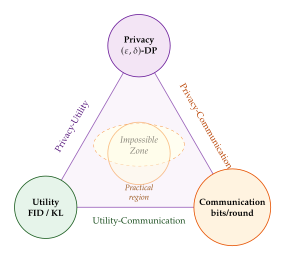
This conjecture is consistent with all known lower bounds for private distributed optimisation, and with the empirical observation that existing federated generative protocols trade off these three properties in predictable ways. However, a formal proof remains elusive, partly because the conjecture requires a unified measure of utility that applies across generative model classes (GANs, VAEs, diffusion models), which are evaluated by fundamentally different metrics.
A weaker version of the conjecture-that no single protocol is uniformly optimal on all three axes-can likely be proved using existing information-theoretic tools. The stronger version, which asserts that the tradeoffs are quantitatively large and unavoidable, would require new lower-bound techniques.
Research Challenge Boxes
We now present three structured research challenge boxes that synthesise multiple open problems and point toward concrete intermediate milestones.
[ enhanced, breakable, colback=exonavybg, colframe=exonavyfg, boxrule=1pt, arc=4pt, title= Research Challenge A: The Federated Diffusion Scaling Benchmark, coltitle=exonavyfg!20!white, fonttitle=, top=10pt, bottom=10pt, left=10pt, right=10pt, before skip=12pt, after skip=12pt ] Goal: Establish the first rigorous scaling benchmark for federated diffusion models, analogous to the scaling laws established for centralised language models.
Methodology:
Train federated DDPM models with parameter counts ranging from to , across clients.
Vary the data heterogeneity using a Dirichlet partition with .
Vary the communication budget bits per round.
Measure generation quality (FID), training efficiency (rounds to target FID), and communication cost (total bits transmitted).
Hypothesised scaling law: for constants and a heterogeneity penalty function satisfying and as .
Expected deliverable: A benchmark suite, baseline implementations of FedAvg-DDPM, FedProx-DDPM, and FedLoRA-DDPM, and an empirical characterisation of the scaling law coefficients.
[ enhanced, breakable, colback=exogreenbg, colframe=exogreenfg, boxrule=1pt, arc=4pt, title= Research Challenge B: Private Federated Molecular Generation for Drug Discovery, coltitle=exogreenfg!20!white, fonttitle=, top=10pt, bottom=10pt, left=10pt, right=10pt, before skip=12pt, after skip=12pt ] Goal: Demonstrate that a federated molecular generative model trained with differential privacy can discover novel drug candidates that outperform models trained on individual client datasets.
Setup: Partition the ChEMBL database into federated clients, each simulating a pharmaceutical company with expertise in a different target class (kinases, GPCRs, ion channels, etc.). Train a federated graph diffusion model with -DP for .
Evaluation metrics:
Validity: fraction of generated SMILES strings that correspond to valid molecules.
Uniqueness: fraction of valid generated molecules not in the training set.
Novelty: fraction of unique molecules not in any client's training set.
Bioactivity: predicted activity against held-out targets using a separately trained QSAR model.
Privacy: membership inference attack AUC against the final model.
Privacy-utility Pareto frontier: Map the tradeoff between and the bioactivity score. The scientific hypothesis is that the federated model achieves higher bioactivity for a given than any single-client model, because federation provides access to a more diverse chemical space.
[ enhanced, breakable, colback=exopurplebg, colframe=exopurplefg, boxrule=1pt, arc=4pt, title= Research Challenge C: Verifiable Federated Unlearning for Generative Models, coltitle=exopurplefg!20!white, fonttitle=, top=10pt, bottom=10pt, left=10pt, right=10pt, before skip=12pt, after skip=12pt ] Goal: Design and implement a cryptographically verifiable unlearning protocol for federated diffusion models that satisfies the trilemma requirements: completeness, efficiency, and verifiability.
Protocol sketch:
During training, the server maintains a cryptographic commitment at each round .
Upon receiving an unlearning request from client , the server computes the gradient of the training loss with respect to using influence functions, and subtracts this influence from .
The server produces a zero-knowledge proof that the updated parameters are consistent with having never trained on .
The proof is published so that any third party can verify the unlearning without accessing .
Key challenge: Influence function computation for large diffusion models is currently , which is infeasible. The research question is whether block-diagonal or low-rank approximations of the Hessian suffice for accurate influence estimation, and whether the resulting approximation errors invalidate the verifiability guarantee.
Evaluation: Test on CelebA-HQ (face generation) with unlearning requests targeting specific identities. Verify using membership inference attacks and identity recognition classifiers.
The Convergence Thesis: FL + Generative + Foundation Models
We close Section Open Problems and Future Directions with a forward-looking synthesis. The three threads of modern AI-federated learning, generative modelling, and foundation models-are not evolving in isolation. They are converging.
Federated learning provides a principled framework for training on distributed, privacy-sensitive data. Generative modelling provides the capacity to learn rich data distributions and to synthesise new examples, serving as both an end goal and a tool for data augmentation. Foundation models provide a powerful, transferable initialisation that dramatically reduces the data and compute requirements for fine-tuning on any specific task or domain.
Key Idea.
The next major paradigm in AI systems will be federated foundation generative models: pre-trained billion-parameter generative models that are continually updated via federated fine-tuning on private, distributed data from millions of edge devices, hospitals, vehicles, and scientific instruments. These models will be capable of generating high-quality synthetic data for any domain, conditioned on locally specified constraints, without ever exposing raw private data. Privacy will be guaranteed by construction via differential privacy and secure aggregation, not bolted on as an afterthought.
This convergence is already visible in early systems. Gboard uses federated learning to update language models on mobile devices. Apple's Neural Engine runs local diffusion models for image enhancement and on-device personalisation. Healthcare consortia use federated learning to train diagnostic models across hospital networks. The synthesis of all three paradigms-federated, generative, and foundation-is the natural next step.
The open problems articulated in this section are not obstacles that will prevent this convergence; they are the research agenda that will make it rigorous and safe. Solving them will require not only new algorithms and theoretical frameworks, but new infrastructure, institutional models, and governance mechanisms. The mathematics and the engineering are ready to begin. The open problems are hard, but they are not intractable.
Insight.
The history of deep learning suggests that the field often advances not by solving existing open problems but by reframing them. Backpropagation did not solve the credit assignment problem; it reframed it. Attention did not solve the long-range dependency problem; it reframed it. The solution to the federated generative trilemma may come from a reframing we cannot yet anticipate.
Comprehensive Exercises and Research Challenges
The following exercises and research challenges are designed to consolidate understanding of the material in this chapter and to push the reader toward independent contribution. The exercises range from mathematical derivations to software implementation, and the research challenges constitute genuine open-ended research projects suitable for a graduate seminar or research internship.
For the exercises, detailed solutions or solution sketches are available in the supplementary material. For the research challenges, there are no predetermined correct answers: the value lies in the process of formulating the problem precisely, implementing a prototype, and interpreting the results.
Exercises
Exercise 61 (FedAvg Derivation and Convergence Analysis).
(a) Starting from the global objective derive the FedAvg update rule. Show that when each client performs exactly one step of gradient descent with learning rate , FedAvg reduces to synchronised SGD.
(b) Assume is -smooth and -strongly convex for all , and that the gradient variance is bounded by . Prove that after rounds of FedAvg with local steps each, the expected gap satisfies where is the weighted average of client models at round . Identify the dominant source of error when .
(c) Suppose client has local objective , where is a client-specific bias term satisfying . Show that FedAvg converges to a biased solution, and compute the bias in terms of the , , and . This is the client drift phenomenon.
Exercise 62 (Non-IID Simulation: Synthetic Dirichlet Partitions).
Let be a set of class labels, and let be a dataset of samples with class distribution where .
(a) Describe the Dirichlet- partitioning scheme for allocating samples to clients. Precisely, if for each class , and the fraction of class- samples allocated to client is , write down the expected number of samples from class at client .
(b) Define the effective heterogeneity of a partition as the average KL divergence between client distributions and the global distribution: where is the class distribution of client under the Dirichlet- partition. Compute and .
(c) Implement the Dirichlet partition in Python/NumPy for CIFAR-10 with clients and . Visualise the resulting class distributions as a stacked bar chart. Report the effective heterogeneity for each .
Exercise 63 (FedGAN Mode Collapse Analysis).
(a) Consider a simple federated GAN with clients. Client 1 holds data from and client 2 holds data from with . The global discriminator is shared, but each client trains a local generator . The generator update is Show that if the discriminator perfectly distinguishes from using the midpoint threshold , then both generators converge to the same mode, either or , regardless of their initialisation.
(b) Propose a modification to the FedGAN objective that encourages diversity between local generators. Specifically, add a repulsion term for some distance function . Analyse whether this term prevents mode collapse in the two-client Gaussian example.
(c) Design an experiment to measure mode collapse in a FedGAN trained on MNIST with clients, each holding only two digit classes. Use the number of distinct modes in the generated distribution (estimated by a pre-trained classifier) as your metric.
Exercise 64 (DP-SGD Noise Calibration for Target ).
(a) Recall that DP-SGD with clipping norm , noise multiplier , sampling rate , and training steps satisfies -differential privacy where is computed via the moments accountant or Renyi DP composition. Using the Gaussian mechanism with -DP and , express the required as a function of , , and . For what value of is achieved?
(b) Consider a federated diffusion model with training samples, batch size , and training steps. Compute the noise multiplier needed to achieve with . Plot the FID score of a DP-trained DDPM on CIFAR-10 as a function of , using the noise values you computed.
(c) The signal-to-noise ratio at step is where is the diffusion loss at noise level . For which diffusion timesteps is the DP noise most damaging? Propose an adaptive noise schedule that allocates more noise to timesteps where the gradient signal is inherently noisy.
Exercise 65 (VAE ELBO Derivation in the Federated Setting).
(a) For a VAE with encoder and decoder , derive the evidence lower bound (ELBO): Starting from , show each algebraic step clearly.
(b) In the federated VAE, client maximises a local ELBO using its own data, and the global model is obtained by averaging client parameters. Formally, define the federated ELBO as Show that is a lower bound on the log-likelihood of the aggregate mixture distribution . What additional assumption is needed?
(c) Suppose encoder parameters are kept locally at each client (personalised), while decoder parameters are shared globally. Derive the update equations for both and under this split federated VAE framework. Discuss when this personalised approach is preferable to a fully shared federated VAE.
Exercise 66 (Gradient Inversion Attack Implementation).
(a) The DLG (Deep Leakage from Gradients) attack reconstructs a private input from an observed gradient by solving Explain why this attack is feasible for small models and batch size 1 but becomes intractable for large models or large batches.
(b) The R-GAP (Recursive Gradient Attack on Privacy) attack improves upon DLG by exploiting the ReLU activation structure to analytically recover the pre-activation values at each layer. For a two-layer fully connected network with ReLU activations: show that the gradient with respect to is where and . Explain how the ReLU structure can be used to recover from when is known.
(c) Implement the DLG attack in PyTorch on MNIST. Train a small CNN, extract the gradient of a single training image, and run the DLG optimisation for 300 iterations. Report the PSNR and SSIM of the reconstructed image. Then add gradient noise with standard deviation and repeat. At what noise level does the attack fail (PSNR below 20 dB)?
Exercise 67 (LoRA Rank Selection and Communication Cost).
(a) In LoRA, a weight matrix is decomposed as where and . The communication cost per round (transmitting and ) is parameters. For a transformer with attention layers, each with query, key, and value matrices of dimension (where is the number of heads), compute the total communication cost as a function of , , , and .
(b) The approximation error of LoRA with rank relative to full fine-tuning is bounded by the sum of the discarded singular values of the optimal weight perturbation : where denotes the -th singular value. Under what distributional assumptions on does rank- LoRA achieve near-zero approximation error?
(c) For a GPT-2 medium model (345M parameters) fine-tuned on a medical text generation task, conduct an ablation study with . Plot perplexity on a held-out medical text corpus versus communication cost in megabytes. Identify the rank that achieves within 5% of the full fine-tuning perplexity at minimum communication cost.
Exercise 68 (FedDDPM Synthetic Auxiliary Data Quality).
(a) The FedDDPM protocol trains a shared diffusion model to generate synthetic auxiliary data . Clients then use to augment local training. Define three metrics for evaluating :
Fidelity: where is a held-out centralised reference set.
Diversity: the number of modes with probability greater than in a pre-trained classifier's softmax distribution over .
Downstream utility: the test accuracy of a classifier trained on evaluated on .
Derive a theoretical relationship between fidelity and downstream utility under the assumption that and are drawn from the same distribution.
(b) In a federated setting with clients and Dirichlet-0.1 partition on CIFAR-10, train a FedDDPM for 200 rounds. Generate synthetic images. For each client , measure the downstream utility (accuracy on the full CIFAR-10 test set) of a ResNet-18 trained on versus alone. Report the average improvement and the variance across clients.
(c) Prove or disprove the following claim: if the FedDDPM model achieves FID on , then the downstream classifier trained on achieves accuracy within of the accuracy of a classifier trained on . What additional assumptions are required?
Exercise 69 (Discrete Diffusion Masking Schedule Design).
In masked discrete diffusion (MDLM/MDDM), tokens are masked at rate and the model learns to unmask them. The forward process is:
(a) Derive the reverse process under this forward process. Show that it factorises over positions and depends only on and .
(b) The training objective for the federated discrete diffusion model is Show that the global federated objective is a valid ELBO for the mixture distribution where is the distribution of .
(c) Compare two masking schedules: (i) linear and (ii) cosine . Which schedule concentrates the unmasking difficulty in earlier or later timesteps? In the federated setting where different clients have different token frequencies, which schedule is more robust to heterogeneous data distributions? Justify with an information-theoretic argument.
Exercise 70 (PRISM Lottery Ticket Probability Analysis).
The PRISM protocol assigns each parameter a retention probability computed from the magnitude of the gradient signal across clients. Specifically, after aggregation: where is the averaged gradient, is a threshold, is a temperature, and is the sigmoid function.
(a) Show that in the IID setting ( where ), the averaged gradient satisfies . What is the expected retention probability as a function of , , , and ?
(b) Define the effective compression ratio of PRISM as , where is the number of parameters. Under a prior on parameter importances, derive as a function of , , , and .
(c) In the non-IID setting, different clients have different gradient magnitudes for the same parameter. Show that the PRISM retention probability overestimates the true importance of parameters that are important for high-weight clients but irrelevant for low-weight clients. Propose a correction that weights client contributions by local dataset size.
Exercise 71 (Federated Unlearning Verification Protocol).
(a) A membership inference attack (MIA) evaluates whether a given sample was in the training set by querying the model. For a generative model , define a score-based MIA: where is a threshold. Explain why a high MIA AUC score on a held-out test set indicates memorisation.
(b) After running a federated unlearning algorithm on client 's data , design a verification protocol using MIA:
Partition into (to be forgotten) and (legitimate to remember).
Compute the MIA AUC for before and after unlearning.
Compute the MIA AUC for before and after unlearning.
A successful unlearning is one where the MIA AUC for drops to approximately 0.5 (random chance) while the AUC for remains above a threshold .
(c) Implement this verification protocol for a FedVAE trained on MNIST. Simulate the unlearning of client 's data by fine-tuning the decoder only on the remaining clients' data. Report the MIA AUC before and after unlearning, and the test ELBO on retained versus unlearned samples. Does simple fine-tuning constitute effective unlearning by your metric?
Exercise 72 (Communication Cost Comparison Across Federated Methods).
Consider a federated training scenario with clients, communication rounds, and a model with parameters. Assume each parameter is represented in 32-bit floating point (4 bytes).
(a) Compute the total communication cost in gigabytes for:
FedAvg (full gradient upload and download each round)
Top- sparsification with (1% of parameters per round)
FedLoRA with rank applied to all linear layers of a transformer with layers, , and 4 matrices per layer
FedDiff (transmitting only noise prediction network gradients, assumed to have parameters)
(b) For each method, compute the communication-utility tradeoff: the ratio of test FID improvement (over the baseline without communication) to total communication cost. Assume:
FedAvg achieves FID improvement FID points.
Top- achieves .
FedLoRA achieves .
FedDiff achieves .
Which method has the best communication-utility tradeoff?
(c) Prove that under a communication budget of total bits and a gradient variance bound , the optimal allocation of bits across rounds is bits per round, and that concentrating all communication in a single round achieves strictly worse convergence.
Research Challenges
The following five research challenges require original implementation, experimental design, and scientific writing. Each challenge is suitable as a course project or research internship deliverable.
Challenge 1 (Build a Minimal FedGAN for MNIST).
Objective: Implement a complete FedGAN system from scratch and systematically investigate the effect of data heterogeneity on mode coverage.
Architecture:
Generator: 4-layer MLP with units, ReLU activations, sigmoid output.
Discriminator: 4-layer MLP with units, LeakyReLU activations.
Shared discriminator, federated via FedAvg.
Local generators per client, aggregated via FedAvg.
Experimental design:
Partition MNIST into clients using Dirichlet- with .
Train for 100 communication rounds with 5 local GAN steps per round.
Measure: FID (using a pre-trained MNIST classifier as the inception model), number of modes covered (digits generated with probability ), and training stability (loss variance).
Compare: FedAvg-GAN versus local-only GAN versus centralised GAN.
Deliverable: A 4-page report with figures showing generated samples at rounds , a table of FID and mode coverage, and a discussion of the mode collapse behaviour observed under highly non-IID conditions.
Challenge 2 (Design a Privacy Attack on a Federated VAE).
Objective: Design and implement a gradient inversion attack targeting a federated VAE, and evaluate the effectiveness of gradient noise as a defence.
Setup:
Train a small VAE (encoder: 2-layer CNN; decoder: 2-layer transposed CNN; latent dimension ) on CelebA-64 using FedAvg with clients.
After training, simulate an honest-but-curious server that observes the gradient updates from one client per round.
Implement three attack strategies: enumerate
Direct reconstruction: minimise the gradient mismatch over the input space.
Latent-space attack: reconstruct the posterior mean from the encoder gradient, then decode to image space.
GAN-prior attack: use a pre-trained GAN to project the reconstruction into a realistic image manifold. enumerate
Defence evaluation: For each attack, measure reconstruction quality (PSNR, SSIM, face recognition accuracy) under:
No defence (baseline).
Gradient clipping (clip norm ).
Gaussian noise ().
Gradient compression (top-1% sparsification).
Deliverable: Reconstruction examples for each attack–defence pair, a quantitative table of PSNR vs. model utility (ELBO), and a recommendation for the minimum noise level that renders all three attacks ineffective while preserving ELBO within 10% of the no-noise baseline.
Challenge 3 (Implement FedDDPM with Synthetic Data Augmentation).
Objective: Implement FedDDPM and demonstrate that synthetic data generated by the federated diffusion model improves downstream classification accuracy on clients with limited local data.
Implementation:
Train a DDPM with a small U-Net backbone ( parameters) using FedAvg on CIFAR-10 partitioned across clients with Dirichlet-0.1.
After 200 rounds, generate of size 50000 images using the aggregated diffusion model.
For each client , train a ResNet-18 classifier on alone and on where is filtered to match the class distribution of .
Compare test accuracy (on the full CIFAR-10 test set) for all three conditions.
Ablation studies:
Effect of .
Effect of filtering strategy: (a) random sampling from ; (b) class-balanced sampling; (c) distribution matching using maximum mean discrepancy.
Effect of diffusion model quality: FID at rounds .
Deliverable: FID curve over training rounds, accuracy improvement table, generated image grid at each training checkpoint, and an analysis of which clients benefit most from synthetic augmentation and why.
Challenge 4 (Create a FedLoRA Training Pipeline).
Objective: Build a complete FedLoRA training pipeline for adapting a pre-trained language model to domain-specific text generation tasks, and characterise the rank-accuracy-communication tradeoff.
Setup:
Use GPT-2 (small, 117M parameters) as the base model.
Simulate federated clients, each holding text from a different domain: medical, legal, financial, scientific, news, fiction, code, social media, dialogue, and poetry. Use domain-specific subsets of The Pile or Common Crawl.
Apply LoRA to the query and value projection matrices in all 12 attention layers with ranks .
Train for 100 federated rounds with 5 local gradient steps per round.
Evaluation:
Perplexity: on held-out test sets for each domain.
Communication cost: total megabytes transmitted per client.
Personalisation: optionally, allow each client to fine-tune the shared LoRA adapter for 10 additional local steps and report perplexity improvement.
Catastrophic forgetting: after federated training, fine-tune the global model on the medical domain for 50 local steps and measure perplexity on the other 9 domains.
Deliverable: Perplexity vs. communication cost Pareto plot, rank ablation table, sample generated texts from each domain, and a discussion of whether the federated model outperforms individually trained domain-specific models at the same communication budget.
Challenge 5 (Propose a Federated Generative Model for Climate Data).
Objective: Design (and, where feasible, prototype) a federated generative model for climate data synthesis, motivated by the challenge that national meteorological agencies cannot share raw station data across borders due to data sovereignty restrictions.
Problem statement: Each of simulated meteorological agencies holds time-series data: temperature, precipitation, wind speed, and humidity at weather stations for a period of 30 years. The agencies wish to train a joint generative model that can simulate realistic global weather patterns and generate synthetic station data for use in climate impact studies.
Design requirements:
Architecture: Propose a generative model architecture suited to multivariate spatio-temporal time series. Candidates include: federated score-based diffusion over graphs, federated normalising flows with temporal conditioning, or federated transformers with spatial attention.
Privacy model: Define what “privacy” means in this context. Should the model prevent reconstruction of individual station records, or should it prevent inference about the statistical climate signature of a particular country or region?
Utility metrics: Define at least three domain-specific metrics for evaluating synthetic climate data quality, e.g., spatial autocorrelation preservation, precipitation frequency distribution, and extreme event (heat wave, drought) frequency.
Communication protocol: Design a communication protocol that accounts for the heterogeneous bandwidth and latency of meteorological agencies in different countries.
Validation: Propose a validation methodology that does not require centralising any real data.
Prototype: Using the ERA5 reanalysis dataset (publicly available), simulate the federated scenario by partitioning ERA5 data by geographic region across 20 simulated agencies. Train a federated score diffusion model on daily temperature fields. Report the continuous ranked probability score (CRPS) of the synthetic climate data relative to held-out ERA5 data.
Deliverable: A 6-page technical report covering the proposed architecture and privacy model, a quantitative evaluation table, a discussion of the practical barriers to deploying such a system in practice (institutional, regulatory, and technical), and a prototype implementation with generated climate data visualisations.
Chapter Summary
This chapter has provided a comprehensive tour of federated generative modelling: the mathematical foundations, the principal algorithms, the privacy and communication tradeoffs, and the open frontiers. We close with two summary boxes that crystallise the chapter's most important insights.
Key Idea.
Three principles underpin all federated generative modelling systems:
1. Data gravity: raw data has a gravitational pull-it stays close to its source. The federated framework accepts this constraint rather than fighting it, treating data locality as a first-class design requirement rather than a limitation to be overcome.
2. The trilemma is real but not fatal: no protocol simultaneously achieves perfect privacy, optimal utility, and minimal communication. Practitioners must understand this tradeoff and make conscious, domain-specific choices about which dimension to prioritise. The choice is never purely technical; it reflects institutional values and regulatory requirements.
3. The generative model is the protocol: in federated generative learning, the model itself serves as a communication medium. By generating synthetic data that can be shared freely, the generative model resolves the privacy-utility tension in a way that discriminative models cannot. This is the deepest reason why generative models are especially valuable in federated settings.
Insight.
The convergence of federated learning, generative modelling, and foundation models is not merely a technical trend-it is a response to a deep social reality. The world's most valuable data is distributed, sensitive, and irreplaceable: medical records, financial transactions, personal communications, scientific measurements. This data cannot and should not be centralised. Yet the patterns in this data, if unlocked, could dramatically accelerate scientific discovery, improve healthcare, and expand access to AI-powered tools.
Federated generative models are the mechanism by which these patterns can be learned and shared without compromising the privacy of individuals or the sovereignty of institutions. The mathematics developed in this chapter-differential privacy, secure aggregation, gradient compression, ELBO decomposition, diffusion score matching-is the formal language in which this mechanism is expressed.
The open problems of Section Open Problems and Future Directions are not obstacles; they are invitations. They mark the boundary between what is known and what remains to be discovered. Solving them is the research agenda of the coming decade.